Controllability analysis of planar snake robots influenced by viscous ground friction

Controllability analysis of planar snake robots influenced byviscous ground friction

Pål Liljebäck, Kristin Y. Pettersen, Øyvind Stavdahl, and Jan Tommy Gravdahl

Abstract—This paper investigates the controllability prop-erties of planar snake robots influenced by viscous groundfriction forces. The paper provides three contributions: 1) Apartially feedback linearized model of a planar snake robotis developed. 2) A stabilizability analysis is presented provingthat any asymptotically stabilizable control law for a planarsnake robot to an equilibrium point must be time-varying. 3) Acontrollability analysis is presented proving that planar snakerobots are not controllable when the viscous ground frictionis uniform, but that a snake robot becomes strongly accessiblewhen the viscous ground friction is non-uniform. The analysisalso shows that the snake robot does not satisfy sufficientconditions for small-time local controllability (STLC).

I. INTRODUCTIONInspired by biological snakes, snake robots carry the

potential of meeting the growing need for robotic mobilityin challenging environments. Snake robots consist of seriallyconnected modules capable of bending in one or more planes.The many degrees of freedom of snake robots make themdifficult to control, but provides traversability in irregularenvironments that surpasses the mobility of the more conven-tional wheeled, tracked and legged forms of robotic mobility.Research on snake robots have been conducted for severaldecades. However, our understanding of snake locomotionso far is for the most part based on empirical studies ofbiological snakes and simulation-based synthesis of relation-ships between parameters of the snake robot. This paperis an attempt to contribute to the understanding of snakerobots by employing well-established system analysis toolsfor investigating fundamental properties of their dynamics.There are several reported works aimed at analysing and

understanding snake locomotion. Gray [1] conducted empiri-cal and analytical studies of snake locomotion already in the1940s. Hirose [2] studied biological snakes and developedmathematical relationships characterizing their motion, suchas the serpenoid curve. Ostrowski [3] considered a particularwheeled snake robot developed by Hirose and studied itscontrollability properties. The results are, however, not veryrelevant to the results of this paper since the snake robotis wheeled and since the analysis was performed on a purekinematic level. Several models of wheel-less snake robotsinfluenced by ground friction have been developed [4]–[10]. However, no formal controllability analysis of snakelocomotion is reported in any of these works. This is also the

Affiliation of Pål Liljebäck is shared between the Departmentof Engineering Cybernetics at the Norwegian University of Scienceand Technology, NO-7491 Trondheim, Norway, and SINTEF ICT,Dept. of Applied Cybernetics, N-7465 Trondheim, Norway. E-mail:[email protected]. Y. Pettersen, Øyvind Stavdahl, and Jan Tommy Gravdahl are

with the Department of Engineering Cybernetics at the NorwegianUniversity of Science and Technology, NO-7491 Trondheim, Norway.E-mail: {Kristin.Y.Pettersen, Oyvind.Stavdahl,Tommy.Gravdahl}@itk.ntnu.no

case for the work by Nilsson [11], where energy argumentsare employed to analyse planar snake locomotion influencedby Coulomb friction. The result is, however, restricted to onespecific motion pattern of a snake robot. The work in [12]presents a feedback linearized model of the joint motion ofa snake robot and studies the controllability of the jointsunder the assumption that one joint is passive. However, theanalysis does not consider the controllability of the positionof the snake robot. There are many reported works on controlof robotic fish and eel-like mechanisms [13]–[15]. Researchon these mechanisms is very relevant to land-based snakerobots. The work in [13] is particularly interesting as itinvestigates the controllability of a robotic fish by employingmathematical tools also employed in this paper. The resultis, unfortunately, not directly applicable to land-based snakerobots due to some fundamental model differences.

This paper provides three contributions. The first contri-bution is a partially feedback linearized model of a planarsnake robot that builds on a model previously presented in[10]. This approach resembles the work in [12]. However,the feedback linearized model in [12] does not include theposition of the snake robot, which is a key ingredient in thispaper. The second contribution is a stabilizability analysis forplanar snake robots that proves that any asymptotically stabi-lizable control law for a planar snake robot to an equilibriumpoint must be time-varying, i.e. not of pure-state feedbacktype (see Theorem 1). This result is valid regardless of whichtype of friction the snake robot is subjected to. Finally, thethird contribution is a controllability analysis for planar snakerobots influenced by viscous ground friction forces. Theanalysis shows that a snake robot is not controllable when theviscous ground friction is uniform (see Theorem 5), but thata snake robot becomes strongly accessible when the viscousground friction is non-uniform (see Theorem 6). The analysisalso shows that the snake robot does not satisfy sufficientconditions for small-time local controllability (see Theorem9). To the authors’ best knowledge, no formal controllabilityanalysis has previously been reported for the position andlink angles of a locomoting snake robot influenced by groundfriction. Note that the work in [12] studies the controllabilityof the joints of a snake robot under the assumption that onejoint is passive. However, the analysis does not consider theposition of the snake.

The paper is organized as follows. Section II gives a briefintroduction to a snake robot model previously presentedin [10]. Section III converts the model from [10] to asimpler form through partial feedback linearization. SectionIV studies stabilizability properties of planar snake robots.Section V presents a controllability analysis of planar snakerobots. Finally, Section VI presents concluding remarks.

The 2009 IEEE/RSJ International Conference onIntelligent Robots and SystemsOctober 11-15, 2009 St. Louis, USA

978-1-4244-3804-4/09/$25.00 ©2009 IEEE 3615

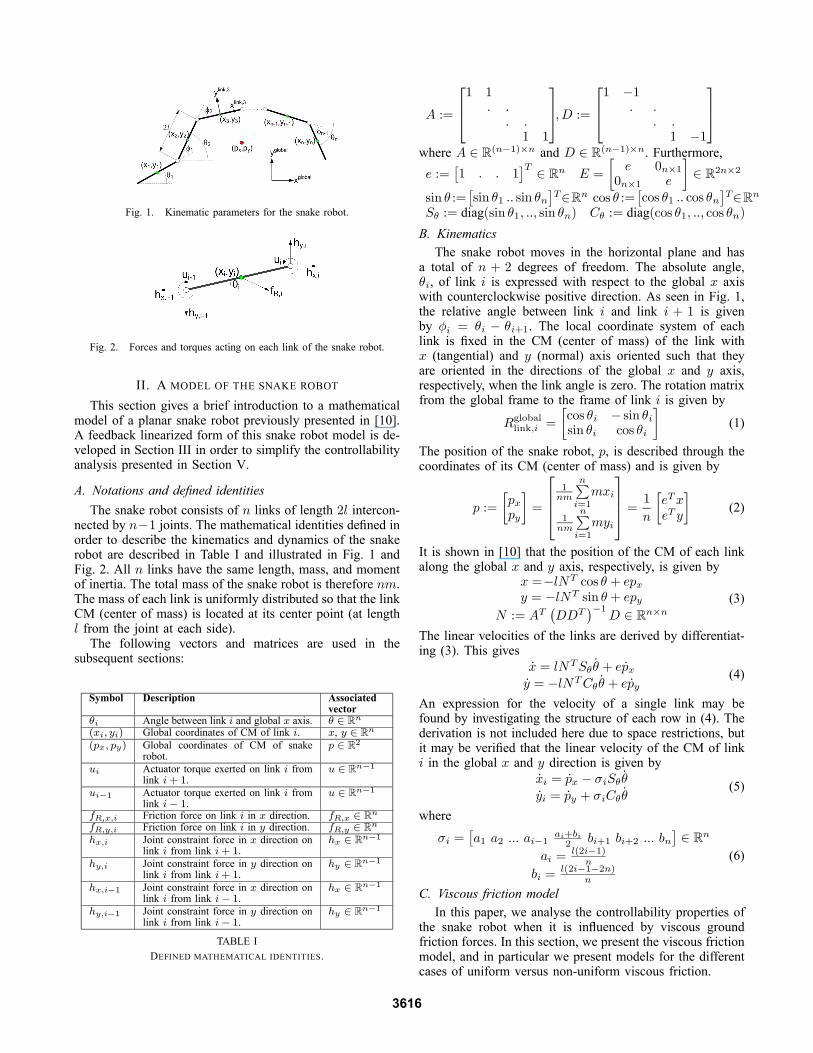
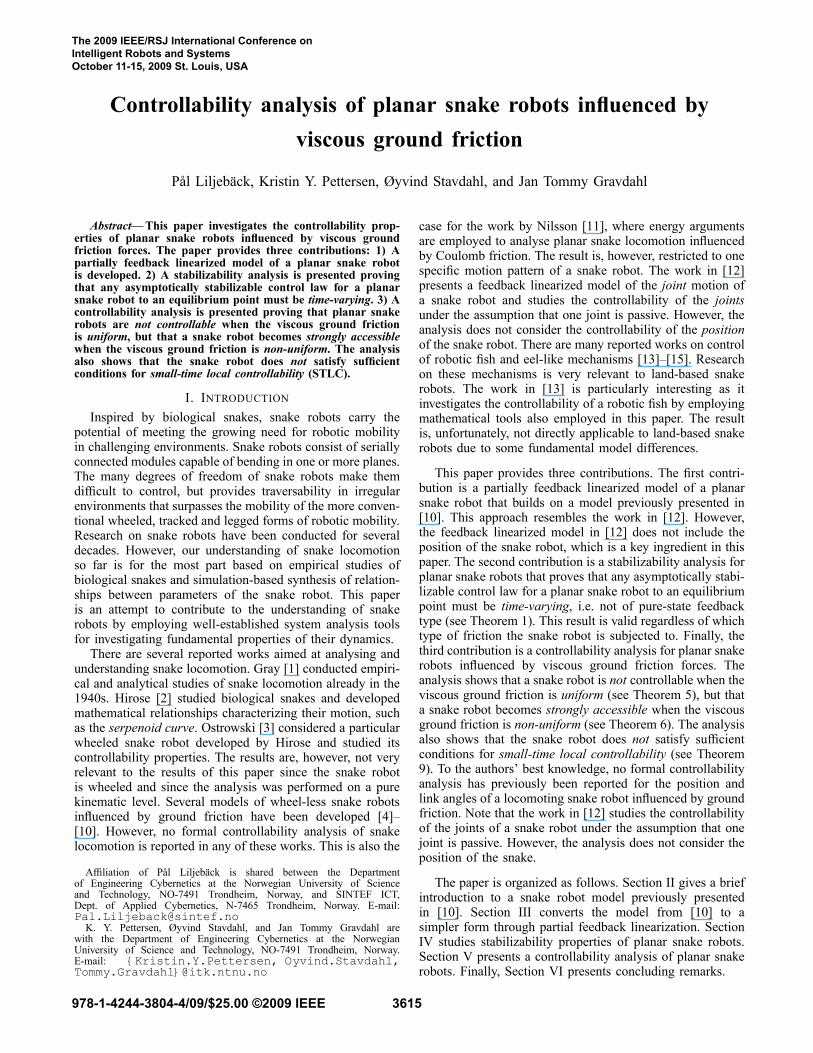
Fig. 1. Kinematic parameters for the snake robot.

Fig. 2. Forces and torques acting on each link of the snake robot.

II. A MODEL OF THE SNAKE ROBOT

This section gives a brief introduction to a mathematicalmodel of a planar snake robot previously presented in [10].A feedback linearized form of this snake robot model is de-veloped in Section III in order to simplify the controllabilityanalysis presented in Section V.

A. Notations and defined identitiesThe snake robot consists of n links of length 2l intercon-

nected by n−1 joints. The mathematical identities defined inorder to describe the kinematics and dynamics of the snakerobot are described in Table I and illustrated in Fig. 1 andFig. 2. All n links have the same length, mass, and momentof inertia. The total mass of the snake robot is therefore nm.The mass of each link is uniformly distributed so that the linkCM (center of mass) is located at its center point (at lengthl from the joint at each side).The following vectors and matrices are used in the

subsequent sections:

Symbol Description Associatedvector

θi Angle between link i and global x axis. θ ∈ Rn(xi, yi) Global coordinates of CM of link i. x, y ∈ Rn(px, py) Global coordinates of CM of snake

robot.p ∈ R2

ui Actuator torque exerted on link i fromlink i+ 1.

u ∈ Rn−1

ui−1 Actuator torque exerted on link i fromlink i− 1.

u ∈ Rn−1

fR,x,i Friction force on link i in x direction. fR,x ∈ RnfR,y,i Friction force on link i in y direction. fR,y ∈ Rnhx,i Joint constraint force in x direction on

link i from link i+ 1.hx ∈ Rn−1

hy,i Joint constraint force in y direction onlink i from link i+ 1.

hy ∈ Rn−1

hx,i−1 Joint constraint force in x direction onlink i from link i− 1.

hx ∈ Rn−1

hy,i−1 Joint constraint force in y direction onlink i from link i− 1.

hy ∈ Rn−1

TABLE IDEFINED MATHEMATICAL IDENTITIES.

A :=

⎡⎢⎣1 1. .

. .1 1

⎤⎥⎦,D :=

⎡⎢⎣1 −1. .

. .1 −1

⎤⎥⎦where A ∈ R(n−1)×n and D ∈ R(n−1)×n. Furthermore,e :=

£1 . . 1

¤T ∈ Rn E =

∙e 0n×1

0n×1 e

¸∈ R2n×2

sin θ :=£sin θ1 .. sin θn

¤T∈Rn cos θ :=

£cos θ1 .. cos θn

¤T∈Rn

Sθ := diag(sin θ1, .., sin θn) Cθ := diag(cos θ1, .., cos θn)B. KinematicsThe snake robot moves in the horizontal plane and has

a total of n + 2 degrees of freedom. The absolute angle,θi, of link i is expressed with respect to the global x axiswith counterclockwise positive direction. As seen in Fig. 1,the relative angle between link i and link i + 1 is givenby φi = θi − θi+1. The local coordinate system of eachlink is fixed in the CM (center of mass) of the link withx (tangential) and y (normal) axis oriented such that theyare oriented in the directions of the global x and y axis,respectively, when the link angle is zero. The rotation matrixfrom the global frame to the frame of link i is given by

Rgloballink,i =

∙cos θi − sin θisin θi cos θi

¸(1)

The position of the snake robot, p, is described through thecoordinates of its CM (center of mass) and is given by

p :=

∙pxpy

¸=

⎡⎢⎢⎣1nm

nPi=1

mxi

1nm

nPi=1

myi

⎤⎥⎥⎦ = 1

n

∙eTxeT y

¸(2)

It is shown in [10] that the position of the CM of each linkalong the global x and y axis, respectively, is given by

x =−lNT cos θ + epxy = −lNT sin θ + epy

N := AT¡DDT

¢−1D ∈ Rn×n

(3)

The linear velocities of the links are derived by differentiat-ing (3). This gives

x = lNTSθθ + epxy = −lNTCθθ + epy

(4)

An expression for the velocity of a single link may befound by investigating the structure of each row in (4). Thederivation is not included here due to space restrictions, butit may be verified that the linear velocity of the CM of linki in the global x and y direction is given by

xi = px − σiSθθ

yi = py + σiCθθ(5)

where

σi =£a1 a2 ... ai−1

ai+bi2 bi+1 bi+2 ... bn

¤∈ Rn

ai =l(2i−1)

n

bi =l(2i−1−2n)

n

(6)

C. Viscous friction modelIn this paper, we analyse the controllability properties of

the snake robot when it is influenced by viscous groundfriction forces. In this section, we present the viscous frictionmodel, and in particular we present models for the differentcases of uniform versus non-uniform viscous friction.

3616

1) Uniform viscous friction: The friction forces are as-sumed to act on the CM of the links only. The uniformviscous friction force on link i in the global x and y directionis proportional to the global velocity of the link and is written

fR,x,i = −cxi = −cpx + cσiSθθ

fR,y,i = −cyi = −cpy − cσiCθθ(7)

where c is the viscous friction coefficient and the expressionfor the link velocity is given by (5). The friction forces onall links may be expressed in matrix form as

fR =

∙fR,xfR,y

¸= −c

∙xy

¸= −c

∙lNTSθθ + epx−lNTCθθ + epy

¸(8)

where the expression for the link velocities is given by (4).We disregard the friction torque caused by a link rotatingwith respect to the ground since this torque only has a minorimpact on the motion of the snake robot.2) Non-uniform viscous friction: Under non-uniform fric-

tion conditions, a link has two viscous friction coefficients, ctand cn, describing the friction force in the tangential (alonglink x axis) and normal (along link y axis) direction of thelink, respectively. Using (1), the friction force on link i inthe global frame as a function of the global link velocity, xiand yi, is given by

fglobalR,i =Rgloballink,i flink,iR,i =−Rgloballink,i

∙ct 00 cn

¸vlink,ii

= −Rgloballink,i

∙ct 00 cn

¸³Rgloballink,i

´T ∙xiyi

¸ (9)

where f link,iR,i and vlink,ii are, respectively, the friction forceand the link velocity expressed in the local link frame.Performing the matrix multiplication and assembling thefriction forces on all links in matrix form gives

fR=−∙ct (Cθ)

2+ cn (Sθ)

2(ct − cn)SθCθ

(ct − cn)SθCθ ct (Sθ)2+ cn (Cθ)

2

∙xy

¸(10)

where fR=£fTR,x fTR,y

¤T ∈ R2n. Note that in the case ofuniform friction (ct = cn = c), the expression for the frictionforces is reduced to (8).

D. Equations of motionThis section presents the equations of motion of the snake

robot in terms of the acceleration of the link angles, θ, andthe acceleration of the CM of the snake robot, p. Thesecoordinates describe all n+ 2 DOFs of the snake robot.The forces and torques acting on link i are visualized

in Fig. 2. The force balance for link i in global framecoordinates is given by

mxi = fR,x,i + hx,i − hx,i−1myi = fR,y,i + hy,i − hy,i−1

(11)

while the torque balance for link i is given byJθi = ui − ui−1

−l sin θi(hx,i + hx,i−1) + l cos θi(hy,i + hy,i−1)(12)

Through straightforward calculations, it is shown in [10] that(11) and (12) may be rewritten for all links and combinedinto the following complete model of the snake robot:

Mθ +Wθ2 − lSθNfR,x + lCθNfR,y = DTu

nmp = ET fR(13)

where θ and p represent the n + 2 generalized coordinatesof the system, θ

2= diag(θ)θ, and

M := JIn×n +ml2 (SθV Sθ + CθV Cθ)W := ml2 (SθV Cθ − CθV Sθ)

N := AT¡DDT

¢−1D

V := AT¡DDT

¢−1A

(14)

III. PARTIAL FEEDBACK LINEARIZATION OF THE MODELThis section transformes the model from [10], which

was summarized in the previous section, to a simplerform through partial feedback linearization. This conversiongreatly simplifies the controllability analysis presented inSection V. Partial feedback linearization of underactuatedsystems was introduced in [16] and consists of linearizing thedynamics corresponding to the actuated degrees of freedomof the system. In this section, we show how a change ofcoordinates makes it possible to employ this methodologyby following the approach presented in [17].

A. Partitioning the model into an actuated and an unactu-ated partBefore partial feedback linearization can be carried out,

the model of the snake robot in (13) must be partitioned intotwo parts representing the actuated and unactuated degreesof freedom, respectively [17]. The acceleration of the CMof the snake robot, p, belongs to the unactuated part since itis not directly influenced by the input, u. The accelerationof the link angles, θ, represent one unactuated degree offreedom and n− 1 actuated degrees of freedom since thereare n link accelerations (θ ∈ Rn) and only n − 1 controlinputs (u ∈ Rn−1). However, it is not possible to partitionthe equation for θ in (13) into an actuated and an unactuatedpart since the matrix DT in front of the control input givesa direct influence between u and all the link accelerations.We therefore seek a form of the model where there is adirect influence between u and only n−1 link accelerations.This is achieved by modifying the choice of generalizedcoordinates from absolute link angles to relative joint angles.The generalized coordinates of the model in (13) are givenby the absolute link angles, θ, and the CM position of thesnake robot, p. We now replace these coordinates with

q =

∙φp

¸∈ Rn+2 (15)

whereφ =

£φ1 φ2 · · · φn−1 θn

¤T ∈ Rn (16)

contains the n − 1 relative joint angles of the snake robotand the absolute link angle, θn ∈ R, of the head link. Therelative joint angles are defined in Fig. 1. The coordinatetransformation between absolute link angles and relative jointangles is easily shown to be given by

θ = Rφ (17)

R =

⎡⎢⎢⎣1 1 1 · · · 1 10 1 1 · · · 1 1...

...0 0 0 · · · 0 1

⎤⎥⎥⎦ ∈ Rn×n (18)

3617

The dynamic model in the new coordinates is found byinserting (17) into (13). This gives

MRφ+W diag³Rφ´Rφ− lSθNfR,x

+lCθNfR,y = DTunmp = ET fR

(19)

where we have used that θ2= diag(θ)θ = diag

³Rφ´Rφ.

Finally, we premultiply the first matrix equation in (19) withRT in order to achieve the desired form of the input mappingmatrix on the right-hand side by making the last of the nequations independent of the control input. This enables usto write the complete model of the snake robot as

M (φ) q +W³φ, φ

´+G (φ) fR

³φ, φ, p

´= Bu (20)

where

q =

∙φp

¸∈ Rn+2 (21)

M (φ) =

∙RTM (φ)R 0n×202×n nmI2

¸(22)

W³φ, φ

´=

"RTW (φ) diag

³Rφ´Rφ

02×1

#(23)

G (φ) =

⎡⎣−lRTSRφN lRTCRφN−eT 01×n01×n −eT

⎤⎦ (24)

B =

∙In−103×n−1

¸(25)

and where SRφ = Sθ and CRφ = Cθ. It is interesting to notethat premultiplying the first matrix equation in (19) with RT

both causes the input mapping matrix to attain a desirableform and produces a symmetrical inertia matrix. Had we leftthe model in the form of (19), the inertia matrix would nothave been symmetrical.The first n−1 equations of (20) represent the dynamics of

the relative joint angles of the snake robot, i.e. the actuateddegrees of freedom of the snake robot. The last threeequations represent the dynamics of the absolute orientationand position of the snake robot, i.e. the unactuated degreesof freedom. The model may therefore be partitioned as

M11qa +M12qu +W 1 +G1fR = u (26)M21qa +M22qu +W 2 +G2fR = 03×1 (27)

where qa =£φ1 · · · φn−1

¤T ∈ Rn−1 represents theactuated degrees of freedom, qu =

£θn px py

¤T ∈R3 represents the unactuated degrees of freedom, M11 ∈Rn−1×n−1,M12 ∈ Rn−1×3,M21 ∈ R3×n−1,M22 ∈ R3×3,W 1 ∈ Rn−1, W 2 ∈ R3, G1 ∈ Rn−1×2n, and G2 ∈ R3×2n.Note that M (φ) only depends on the relative joint anglesof the snake robot and not on the absolute orientation of thehead link, θn. Formally, this is a result of the fact that θn isa cyclic coordinate [18]. Less formally, this is quite obvioussince it would not be reasonable that the inertial properties ofa planar snake robot is dependent on how the snake robot isoriented in the plane. We therefore have that M =M (qa).

B. Partial feedback linearizationWe are now ready to present an input transformation that

linearizes the dynamics of the actuated degrees of freedomin (26). M22 is an invertible 3× 3 matrix as a consequenceof the uniform positive definiteness of the complete systeminertia matrix, M (qa). We may therefore solve (27) for quas

qu = −M−122

¡M21qa +W 2 +G2fR

¢(28)

Inserting (28) into (26) gives³M11 −M12M

−122 M21

´qa +W 1 +G1fR

−M12M−122

¡W 2 +G2fR

¢= u

(29)

Consequently, the following linearizing controlleru =

³M11 −M12M

−122 M21

´v +W 1

+G1fR −M12M−122

¡W 2 +G2fR

¢ (30)

enables us to rewrite (26) and (27) asqa = v (31)qu = A (q, q) + B (qa) v (32)

whereA (q, q) = −M−122

¡W 2 +G2fR

¢∈ R3 (33)

B (qa) = −M−122 M21 ∈ R3×n−1 (34)

This model may be written in the standard form of a control-affine system by defining x1 = qa, x2 = qu, x3 = qa,x4 = qu, and x =

£xT1 xT2 xT3 xT4

¤T ∈ R2n+4. Thisgives

x =

⎡⎢⎣ x3x4

0n−1×1A (x)

⎤⎥⎦+⎡⎢⎣0n−1×n−103×n−1

In−1B (x1)

⎤⎥⎦ v = f (x) +n−1Xj=1

gj (x1) vj

(35)where

f (x) =

⎡⎢⎣ x3x4

0n−1×1A (x)

⎤⎥⎦ , gj (x1) =⎡⎢⎣0n−1×103×1

ejBj (x1)

⎤⎥⎦ (36)

and where ej denotes the jth standard basis vector in Rn−1(the jth column of In−1) and Bj (x1) denotes the jth columnof B (x1).

IV. STABILIZABILITY PROPERTIES OF PLANAR SNAKEROBOTS

This section presents and proves a fundamental theoremconcerning the properties of an asymptotically stabilizablecontrol law for snake robots to any equilibrium point. From(35), the model of the snake robot is given by

x =

⎡⎢⎣x1x2x3x4

⎤⎥⎦ =⎡⎢⎣ x3

x4v

A (x) + B (x1) v

⎤⎥⎦ (37)

The equation (37) maps the state, x, and the controllerinput, v, of the snake robot into the resulting deriva-tive of the state vector, x. For any equilibrium point(x1 = xe1, x2 = xe2, x3 = 0, x4 = 0), where (xe1, xe2) is the

3618

configuration of the system at the equilibrium point, we havethat x = 0.A well-known result by Brockett [19] states that a neces-

sary condition for the existence of a time-invariant (i.e. notexplicitly dependent on time) continuous state feedback law,v = v (x), that makes (xe1, xe2, 0, 0) asymptotically stable, isthat the image of the mapping (x, v) 7→ x contains someneighbourhood of x = 0. A result by Coron and Rosier[20] states that a control system that can be asymptoticallystabilized (in the Filippov sense [20]) by a time-invariantdiscontinuous state feedback law can be asymptotically sta-bilized by a continuous time-varying state feedback law. If,moreover, the control system is affine (i.e. linear with respectto the control input), then it can be asymptotically stabilizedby a time-invariant continuous state feedback law. We nowemploy these results to prove the following fundamentaltheorem for planar snake robots:Theorem 1: An asymptotically stabilizable control law

for a planar snake robot described by (37) to any equilibriumpoint must be time-varying, i.e. of the form v = v (x, t).

Proof: The result by Brockett [19] states that themapping (x1, x2, x3, x4, v) 7→ (x3, x4, v,A (x) + B (x1) v)must map an arbitrary neighbourhood of(x1 = xe1, x2 = xe2, x3 = 0, x4 = 0, v = 0) onto a neigh-bourhood of (x3 = 0, x4 = 0, v = 0,A (x) + B (x1) v = 0).For this to be true, points of the form(x3 = 0, x4 = 0, v = 0,A (x) + B (x1) v = ) must becontained in this mapping for some arbitrary 6= 0because points of this form are contained in everyneighbourhood of x = 0. However, these points do notexist for the system in (37) because x3 = 0, x4 = 0,and v = 0 means that A (x) + B (x1) v = 0 6= . Hence,the snake robot cannot be asymptotically stabilized to(x1 = xe1, x2 = xe2, x3 = 0, x4 = 0) by a time-invariantcontinuous state feedback law. Moreover, since the systemin (37) is affine and cannot be asymptotically stabilized bya time-invariant continuous state feedback law, the result byCoron and Rosier [20] proves that the system can neither beasymptotically stabilized by a time-invariant discontinuousstate feedback law. We can therefore conclude that anasymptotically stabilizable control law for a planar snakerobot to any equilibrium point must be time-varying, i.e. ofthe form v = v (x, t).Remark 2: Theorem 1 is independent of the choice of

friction model and applies to any planar snake robot de-scribed by a friction model with the property that A (xe) = 0for any equilibrium point xe.

V. CONTROLLABILITY ANALYSIS OF PLANAR SNAKEROBOTS

This section studies the controllability of planar snakerobots influenced by viscous ground friction forces. The firstsubsection presents a brief summary of selected tools foranalyzing controllability of nonlinear systems. Most literarysources of this theory present the theory in the contextof complex mathematical notations and terminologies. Thesummary given below is therefore formulated in an intuitiveform that aims to be easily understandable, and thus hope-fully can be a valuable contribution to readers that want anintroduction to nonlinear controllability analysis.

A. Controllability concepts for nonlinear systemsAnalyzing the controllability of a linear system is easy

and involves a simple test (the Kalman rank condition [21])on the constant system matrices. However, studying thecontrollability of a nonlinear system is far more complexand constitutes an active area of research. In the following,we summarize important controllability concepts for control-affine nonlinear systems, i.e. systems of the form

x = f (x) +mPj=1

gj (x) vj , x ∈ Rn , v ∈ Rm (38)

where the vector fields of the system are the drift vector field,f (x), and the control vector fields, gj (x), j ∈ [1, ..,m].A nonlinear system is said to be controllable if there exist

admissible control inputs that will bring the system betweentwo arbitrary states in finite time. However, conditions forthis kind of controllability that are both necessary andsufficient do not exist. Nonlinear controllability is insteadtypically analyzed by investigating the local behaviour ofthe system near equilibrium points.The simplest approach to studying controllability of a

nonlinear system is to linearize the system about an equilib-rium point, xe. If the linearized system satisfies the Kalmanrank condition at xe, the nonlinear system is controllablein the sense that the set of states that can be reached fromxe contains a neighborhood of xe [21]. Unfortunately, manyunderactuated systems do not have a controllable lineariza-tion. Moreover, a nonlinear system can be controllable eventhough its linearization is not.A necessary (but not sufficient) condition for controlla-

bility from a state x0 (not necessarily an equilibrium) is thatthe nonlinear system satisfies the Lie algebra rank condition(LARC), also called the accessibility rank condition [21]. Ifthis is the case, the system is said to be locally accessiblefrom x0. This property means that the space that the systemcan reach within any time T > 0 is fully n-dimensional, i.e.the reachable space from x0 has a dimension equal to thedimension of the state space. A slightly stronger propertyis strong accessibility, which means that the space that thesystem can reach in exactly time T for any T > 0 is fullyn-dimensional.Accessibility of a nonlinear system is investigated by

computing the accessibility algebra, here denoted ∆, of thesystem. Computation of ∆ requires knowledge of the Liebracket [21], which is now briefly explained. The drift andcontrol vector fields of the nonlinear system (38) indicatedirections in which the state x can move. These directionswill generally only span a subset of the complete state space.However, through combined motion along two or more ofthese vector fields, it is possible for the system to movein directions not spanned by the original system vectorfields. The Lie bracket between two vector fields Y and Zproduces a new vector field defined as [Y,Z] = ∂Z

∂x Y −∂Y∂x Z.

When Y and Z are any of the system vector fields, the Liebracket [Y,Z] approximates the net motion produced whenthe system follows these two vector fields in an alternatingfashion. The classical example is parallel parking with a car,where sideways motion of the car may be achieved throughan alternating turning and forward/backward motion. Notethat Lie brackets can be computed from other Lie brackets,

3619

thereby producing nested Lie brackets. The accessibilityalgebra, ∆, is a set of vector fields composed of the systemvector fields, f and gj , the Lie brackets between the systemvector fields, and also higher order Lie brackets generatedby nested Lie brackets. The LARC is satisfied at x0 if thevector fields in ∆ (x0) span the entire n-dimensional statespace (span (∆) = n). The following result is proved in [21]:Theorem 3: The system (38) is locally accessible from

x0 if and only if the LARC is satisfied at x0. The system islocally strongly accessible if the drift field f by itself (i.e.unbracketed) is not included in the accessibility algebra.Accessibility does not imply controllability since it only

infers conclusions on the dimension of the reachable spacefrom x0. Accessibility is, however, a necessary (but not suf-ficient) condition for small-time local controllability (STLC)[22]. STLC is desirable since it is in fact a stronger propertythan controllability. If a system is STLC, then the controlinput can steer the system in any direction in an arbitrarilysmall amount of time. For second-order systems, STLC istherefore only possible from equilibrium states since it is notpossible for a second-order system to instantly move in onedirection if it already has a velocity in the opposite direction.Only sufficient (not necessary) conditions for STLC exist.Sussmann presented sufficient conditions for STLC in

[22]. These results were later extended by Bianchini andStefani [23]. We now summarize these conditions. For anyLie bracket term B generated from the system vector fields,define the θ-degree of B, denoted δθ (B), and the l-degreeof B, denoted δl (B), as

δθ (B)=1

θδ0 (B)+

mXj=1

δj (B) , δl (B)=mXj=0

ljδj (B) (39)

respectively, where δ0 (B) is the number of times the driftvector field f appears in the bracket B, δj (B) is the numberof times the control vector field gj appears in the bracket B,θ is an arbitrary number satisfying θ ∈ [1,∞), and lj is anarbitrary number satisfying lj ≥ l0 ≥ 0, ∀ j ∈ {0, ..,m}.The bracket B is said to be bad if δ0 (B) is odd andδ1 (B) , ..., δm (B) are all even. A bracket is good if it isnot bad. As an example, we have that the bracket [gj , [f, gk]]is bad for j = k and good for j 6= k. This classification ismotivated by the fact that a bad bracket may have directionalconstraints. E.g. the drift vector f is bad because it onlyallows motion in its positive direction and not in its negativedirection, −f . A bad bracket is said to be θ-neutralized (resp.l-neutralized) if it can be written as a linear combination ofbrackets of lower θ-degree (resp. l-degree). The Sussmanncondition and the Bianchini and Stefani condition for STLCare now combined in the following theorem:Theorem 4: The system (38) is small-time locally con-

trollable (STLC) from an equilibrium point xe ( f (xe) = 0)if the LARC is satisfied at xe and either all bad bracketsare θ-neutralized (Sussmann [22]) or all bad brackets arel-neutralized (Bianchini and Stefani [23]).

B. Controllability with uniform viscous frictionWe begin the controllability analysis of the snake robot

by first assuming that the viscous ground friction is uniform.In this case, it turns out that the equations of motion takeon a particularly simple form that enables us to study

controllability through pure inspection of the equations ofmotion. From (13) we have that the acceleration of the CMof the snake robot is given by∙

pxpy

¸=

∙1nmeT fR,x1nmeT fR,y

¸=

1

nm

⎡⎢⎢⎣nPi=1

fR,x,inPi=1

fR,y,i

⎤⎥⎥⎦ (40)

Inserting (7) into (40) gives∙pxpy

¸=

c

nm

⎡⎢⎢⎣−npx +µ

nPi=1

σi

¶Sθθ

−npy −µ

nPi=1

σi

¶Cθθ

⎤⎥⎥⎦ = − c

m

∙pxpy

¸(41)

because it may be shown thatnPi=1

σi = 0. This enables us to

state the following theorem:Theorem 5: A planar snake robot influenced by uniform

viscous ground friction is not controllable.Proof: In order to control the position, the snake robot

must accelerate its CM (center of mass). From (41) it is clearthat the CM acceleration is proportional to the CM velocity.If the snake robot starts from rest (p = 0), it is thereforeimpossible to achieve acceleration of the CM. The position ofthe snake robot is in other words completely uncontrollablein this case, which renders the snake robot uncontrollable.

C. Controllability with non-uniform viscous frictionThe equations of motion of the snake robot in (35) become

far more complex under non-uniform friction conditions.We therefore employ the controllability concepts presentedin Section V-A and begin by computing the Lie bracketsof the system vector fields. The drift and control vectorfields of the snake robot are given in (36). As explainedin Section V-A, Lie bracket computation involves partialderivatives of the components of the vector fields. Thesecomputations can be carried out without dealing with thecomplex expressions contained in A (x) and B (x1) givenby (33) and (34), respectively, since we only need to knowwhich variables each row of the vector fields depend on.As an example, consider column j of B (x1). Since weknow that it only depends on x1, we may immediately write∂Bj(x1)

∂x =h∂Bj(x1)∂x1

03×n+5

i. This methodology enables

us to compute the following Lie brackets of the system vectorfields (evaluated at an equilibrium point):

[f, gj ]q=0

=

⎡⎢⎣ −ej−Bj0n−1×1−Cj

⎤⎥⎦ , [f, [f, gj ]]q=0=⎡⎢⎢⎣0n−1×1Cj

0n−1×1∂A∂x4Cj

⎤⎥⎥⎦[[f, gj ] , [f, gk]]

q=0=

⎡⎢⎣0n−1×1Djk

0n−1×1Ejk

⎤⎥⎦(42)

where j, k ∈ {1, ..., n− 1} andCj = ∂A

∂x3ej +

∂A∂x4Bj , Djk =

∂Bk∂x1

ej − ∂Bj∂x1

ek

Ejk= ∂Ck∂x1

ej−∂Cj∂x1ek+

∂Ck∂x2Bj−∂Cj∂x2

Bk+∂Ck∂x4Cj−∂Cj∂x4

Ck(43)

The Lie brackets have been evaluated at zero velocity (q = 0)since we are interested in controllability from an equilibrium

3620

point. The above vector fields represent our choice of vectorfields to be contained in the accessibility algebra, ∆, ofthe system. To construct ∆ of full rank, we need to find(2n+ 4) independent vector fields since the snake robot hasa (2n+ 4)-dimensional state space. Each of the four typesof vector fields above represent (n−1) vector fields. Solving4(n − 1) ≥ 2n + 4 gives that our analysis is only valid ifthe snake robot has n ≥ 4 links. This is a mild requirement,however, since a snake robot generally will have more thanfour links. In the remainder of this section, we assumethat the snake robot consists of exactly n = 4 links (andthereby n−1 = 3 active joints) and argue that the followingcontrollability results will also be valid for snake robots withmore links. In particular, a snake robot with n > 4 links canbehave as a snake robot with n = 4 links by fixing (n− 4)joint angles at zero degrees and allowing the remaining threejoint angles to move. This means that controllability of thesnake robot with n = 4 is a sufficient although not necessarycondition for controllability of snake robots with n > 4.With n = 4 links, the system has a (2n+ 4) = 12-

dimensional state space. The system satisfies the Lie algebrarank condition (LARC) if the above vector fields span a12-dimensional space. We therefore assemble the 12 vectorfields into the following matrix, which represents the acces-sibility algebra of the system evaluated at an equilibriumpoint xe:

∆ (xe) = [g1, g2, g3, [f, g1] , [f, g2] , [f, g3] ,[f, [f, g1]] , [f, [f, g2]] , [f, [f, g3]] ,

[[f, g1] , [f, g2]] , [[f, g1] , [f, g3]] , [[f, g2] , [f, g3]]]

=

⎡⎢⎢⎣03×3 −I3 03×3 03×103×3 −B C DI3 03×3 03×3 03×1B −C ∂A

∂x4C E

⎤⎥⎥⎦ ∈ R12×12(44)

where

C = ∂A∂x3

+ ∂A∂x4B ∈ R3×3

D =£D12 D13 D23

¤, E =

£E12 E13 E23

¤ (45)

We now state the following theorem regarding the acces-sibility of the snake robot:Theorem 6: A planar snake robot with n ≥ 4 links

influenced by non-uniform viscous ground friction (ct 6= cn)is locally strongly accessible from any equilibrium point xe

(q = 0) satisfying det (C) 6= 0 and det³E− ∂A

∂x4D´6= 0,

where det (∗) denotes the determinant evaluated at xe.Proof: By Theorem 3, the system is locally strongly

accessible from xe if ∆ (xe), given by (44), has full rank,i.e. spans a 12-dimensional space. The proof is completeif we can show that this is the case as long as det (C) 6=0 and det

³E− ∂A

∂x4D´6= 0 at xe. The matrix ∆ (xe) has

full rank when all its columns are linearly independent. Byinvestigating the particular structure of ∆ (xe), we see thatthe first and third row contains an identity matrix and thenzeros in the remaining elements of these rows. It is thereforeimpossible to write the columns containing the two identitymatrices as linear combinations of other columns. We cantherefore conclude that any linear dependence between thecolumns of ∆ (xe) must be caused by linear dependencebetween the columns of the following submatrix of ∆ (xe):

e∆ (xe) = ∙ C D∂A∂x4C E

¸∈ R6×6 (46)

Linear dependence between columns of a square matrixcauses its determinant to become zero. We therefore calculatethe determinant of e∆ (xe) by employing the following well-known mathematical relationship concerning the determinantof a block matrix (see e.g. [24]):

det

µ∙A BC D

¸¶= det (A) det

¡D − CA−1B

¢(47)

where A and D are any square matrices and A is non-singular. This gives

det³e∆ (xe)´ = det (C) detµE− ∂A

∂x4D¶

(48)

The determinant of e∆ (xe) is zero when det (C) = 0 orwhen det

³E− ∂A

∂x4D´= 0. This means that e∆ (xe), and

thereby also ∆ (xe), has full rank whenever det (C) 6= 0 anddet

³E− ∂A

∂x4D´6= 0. This completes the proof.

The requirement regarding the two determinants in Theo-rem 6 is not very restrictive, but implies that the snake robotcan attain configurations that are singular, i.e. certain shapesof the snake robot are obstructive from a control perspectivesince the dimension of the reachable space from theseconfigurations is not full-dimensional. Note that we onlyconsider joint angles satisfying φi < |90◦| since larger jointangles are not common for snake robots. Our investigationsso far indicate that the only singular configurations of aplanar snake robot are configurations where all joint anglesare equal (φ1 = φ2 = ... = φn−1). These are postures wherethe snake robot is either lying straight or forming an arcof a circle. Such postures are easily avoided during snakelocomotion. Unfortunately, the expressions for det (C) anddet

³E− ∂A

∂x4D´are extremely complex and hard to analyze,

even when employing a mathematical software tool such asMatlab Symbolic Math Toolbox. At this point, we thereforecannot rule out the possibility that other singular posturesalso exist, but we consider it unlikely. We may anyhow statethe following corollary:Corollary 7: Theorem 6 is not satisfied at equilibrium

points where all relative joint angles are equal (φ1 = φ2 =... = φn−1).

Proof: It is straightforward to verify with a mathemati-cal software tool such as Matlab Symbolic Math Toolbox thatdet (C)

¯φ1=φ2=...=φn−1

= 0, thus violating the conditions inTheorem 6.Remark 8: Corollary 7 implies that the joint angles of a

snake robot should be out of phase during snake locomotion.This claim has been stated in several previous works [1], [2],[4], [7], but no formal mathematical proof was given.We now show that the snake robot does not satisfy suffi-

cient conditions for small-time local controllability (STLC):Theorem 9: A planar snake robot with n ≥ 4 links

influenced by viscous ground friction does not satisfy the suf-ficient conditions for small-time local controllability (STLC)stated in Theorem 4.

Proof: The proof is complete if we can show that thereare bad brackets of the system vector fields that cannot be

3621

neither θ-neutralized nor l-neutralized (see Theorem 4). Thebad brackets with the lowest θ-degree and the lowest l-degree(except for f , which vanishes at any equilibrium point) are[gj , [f, gj ]], j ∈ {1, 2, 3}. Theorem 4 requires these vectorsto be written as linear combinations of good brackets witheither lower θ-degree or lower l-degree. The only such goodbrackets are gj , [f, gj ] , [f, [f, gj ]] , .., [f, [· · · [f, gj ]] · · · ], j ∈{1, 2, 3}. Brackets of the form [gk, gj ] are not consideredbecause [gk, gj ] = 0, j, k ∈ {1, 2, 3}. For a proper choice ofθ and lj , j ∈ {0, 1, 2, 3}, these brackets have both lower θ-degree and lower l-degree. It is straightforward to verify that[gj , [f, gj ]] ∈ R2n+4=12 is a vector of all zeros except for el-ement number 2n+2 = 10. The only way to write this vectoras a linear combination of the good brackets listed above isif these good brackets span the entire 12-dimensional statespace. This is not the case, however, because the vectors[f, [f, gj ]] , .., [f, [· · · [f, gj ]] · · · ] are linearly dependent, ascan be seen by assembling the following matrix:

[[f, [f, gj ]] , [f, [f, [f, gj ]]] , [f, [f, [f, [f, gj ]]]] , · · · ]

=

⎡⎢⎢⎢⎢⎣03×3 03×1 03×1 · · ·C − ∂A

∂x4C

³∂A∂x4

´2C · · ·

03×3 03×1 03×1 · · ·∂A∂x4C −

³∂A∂x4

´2C

³∂A∂x4

´3C · · ·

⎤⎥⎥⎥⎥⎦ (49)

and noting that the fourth row is a multiple of the secondrow. For the system in (35), it is therefore not possible toneither θ-neutralize nor l-neutralize the bad brackets of thesystem. This completes the proof.Note that necessary conditions for STLC do not exist.

The snake robot may therefore be STLC even though thesufficient conditions in Theorem 4 are violated.We end this section with a note on Theorem 6. This the-

orem clearly shows that non-uniform friction is an importantproperty for a snake robot. In the snake robot literature, it iscommon for snake robots to possess the property cn À ct.The extreme case of this property is realized by installingpassive wheels along the snake body since this ideally meansthat ct = 0 and cn = ∞. However, from Theorem 6 itis clear that the only requirement for strong accessibilityis that the friction coefficients are not equal. The propertyct > cn is therefore also valid. This means that the passivewheels commonly mounted tangential to the snake body mayequally well be mounted transversal to the snake body. Theresulting motion will off course be different, but the strongaccessibility property is still preserved.

VI. CONCLUSIONThis paper has investigated the controllability properties

of planar snake robots influenced by viscous ground frictionforces. The first contribution of the paper is a partiallyfeedback linearized model of a planar snake robot. Thesecond contribution is a stabilizability analysis proving thatany asymptotically stabilizable control law for a planar snakerobot to an equilibrium point must be time-varying. Thisresult is valid regardless of which type of friction the snakerobot is subjected to. The third and final contribution is acontrollability analysis proving that planar snake robots arenot controllable when the viscous ground friction is uniform,but that a snake robot becomes strongly accessible when the

viscous ground friction is non-uniform. This analysis showedthat the joint angles of a snake robot should be out of phaseduring snake locomotion. The analysis also showed that thesnake robot does not satisfy sufficient conditions for small-time local controllability (STLC).

REFERENCES[1] J. Gray, “The mechanism of locomotion in snakes,” J. Exp. Biol.,

vol. 23, no. 2, pp. 101–120, 1946.[2] S. Hirose, Biologically Inspired Robots: Snake-Like Locomotors and

Manipulators. Oxford: Oxford University Press, 1993.[3] J. P. Ostrowski, “The mechanics and control of undulatory robotic

locomotion,” Ph.D. dissertation, California Institute of Technology,1996.

[4] T. Kane and D. Lecison, “Locomotion of snakes: A mechanical‘explanation’,” Int. J. Solids Struct., vol. 37, no. 41, pp. 5829–5837,October 2000.

[5] S. Ma, “Analysis of creeping locomotion of a snake-like robot,” Adv.Robotics, vol. 15, no. 2, pp. 205–224, 2001.

[6] M. Saito, M. Fukaya, and T. Iwasaki, “Serpentine locomotion withrobotic snakes,” IEEE Contr. Syst. Mag., vol. 22, no. 1, pp. 64–81,February 2002.

[7] G. P. Hicks, “Modeling and control of a snake-like serial-link struc-ture,” Ph.D. dissertation, North Carolina State University, 2003.

[8] P. Liljebäck, Ø. Stavdahl, and K. Y. Pettersen, “Modular pneumaticsnake robot: 3D modelling, implementation and control,” in Proc. 16thIFAC World Congress, July 2005.

[9] A. A. Transeth, R. I. Leine, Ch.. Glocker, and K. Y. Pettersen,“Non-smooth 3D modeling of a snake robot with frictional unilateralconstraints,” in Proc. IEEE Int. Conf. Robotics and Biomimetics,Kunming, China, Dec 2006, pp. 1181–1188.

[10] P. Liljebäck, K. Y. Pettersen, and Ø. Stavdahl, “Modelling and controlof obstacle-aided snake robot locomotion based on jam resolution,” inProc. IEEE Int. Conf. Robotics and Automation, 2009, pp. 3807–3814.

[11] M. Nilsson, “Serpentine locomotion on surfaces with uniform friction,”in Proc. IEEE/RSJ Int. Conf. Intelligent Robots and Systems, 2004, pp.1751–1755.

[12] J. Li and J. Shan, “Passivity control of underactuated snake-likerobots,” in Proc. 7th World Congress on Intelligent Control andAutomation, June 2008, pp. 485–490.

[13] K. Morgansen, V. Duidam, R. Mason, J. Burdick, and R. Murray,“Nonlinear control methods for planar carangiform robot fish loco-motion,” in Proc. IEEE Int. Conf. Robotics and Automation, vol. 1,2001, pp. 427–434 vol.1.

[14] P. Vela, K. Morgansen, and J. Burdick, “Underwater locomotion fromoscillatory shape deformations,” in Proc. IEEE Conf. Decision andControl, vol. 2, Dec. 2002, pp. 2074–2080 vol.2.

[15] K. McIsaac and J. Ostrowski, “Motion planning for anguilliformlocomotion,” IEEE Trans. Robot. Autom., vol. 19, no. 4, pp. 637–625,August 2003.

[16] Y.-L. Gu and Y. Xu, “A normal form augmentation approach toadaptive control of space robot systems,” in Proc. IEEE Int. Conf.Robotics and Automation, vol. 2, May 1993, pp. 731–737.

[17] M. Reyhanoglu, A. van der Schaft, N. McClamroch, and I. Kol-manovsky, “Dynamics and control of a class of underactuated me-chanical systems,” IEEE Transactions on Automatic Control, vol. 44,no. 9, pp. 1663–1671, September 1999.

[18] H. Goldstein, C. Poole, and J. Safko, Classical Mechanics - ThirdEdition. Addision Wesley, 2002.

[19] R. Brockett, “Asymptotic stability and feedback stabilization,” Differ-ential Geometric Control Theory, pp. 181–191, 1983.

[20] J.-M. Coron and L. Rosier, “A relation between continuous time-varying and discontinuous feedback stabilization,” J. of MathematicalSystems, Estimation, and Control, vol. 4, no. 1, pp. 67–84, 1994.

[21] H. Nijmeijer and A. v. d. Schaft, Nonlinear Dynamical ControlSystems. New York: Springer-Verlag, 1990.

[22] H. J. Sussmann, “A general theorem on local controllability,” SIAMJournal on Control and Optimization, vol. 25, no. 1, pp. 158–194,1987.

[23] R. M. Bianchini and G. Stefani, “Graded approximations and control-lability along a trajectory,” SIAM J. Control and Optimization, vol. 28,no. 4, pp. 903–924, 1990.

[24] D. A. Harville, Matrix Algebra From a Statistician’s Perspective.Springer, 2000.

3622