Conflict Areas for Macroscopic Models in Dynamic Traffic Assignment

Conflict Areas for Macroscopic Models in

Dynamic Traffic Assignment

Daniele Tiddi, Bojan Kostic, Guido Gentile

DICEA, Sapienza University of Rome

Abstract

Intersections are the most critical elements of road networks, especially in urban contexts. In

the representation of junctions for macroscopic DTA models, the usual assumption is that

every conflict among intersecting traffic streams of different manoeuvres is fully solved by

traffic signals. This simplifies the simulation of intersections, given that only merging and

diversions are to be reproduced, and most DTA models are capable of addressing these basic

topologies. However, quite often in practice we have intersecting manoeuvres that comply

with some precedence and/or gap-acceptance rule, even in signalized junctions. These

phenomena are very well tackled by micro-simulation models, while limited research has

been produced to successfully and efficiently represent nodes with conflict areas in

macroscopic models for Dynamic Traffic Assignment. This article addresses the above issue,

providing a new formulation for conflicting traffic streams in the context of the General Link

Transmission Model. To this end, the merging model with priorities is extended by

associating a capacity to each manoeuvre, while the scarce resource to be split becomes the

time of the conflict area. A specific parameter to reproduce different driver behaviour from

polite to aggressive is also introduced. The model has been implemented in the software for

Dynamic Traffic Assignment called TRE. Numerical results are presented to show how the

model works for different combinations of flows, capacities and priorities.

Keywords: junctions with conflicting manoeuvres, Link Transmission Model, Dynamic

Network Loading, turn priorities, polite vs. aggressive driver behavior.

1 Introduction

Dynamic Traffic Assignment (DTA) has recently received a considerable attention as an

effective tool for real-time traffic management [Gen11]. Reliable DTA models are necessary

for realistic estimation of current traffic states and prediction of traffic conditions in the near

future.

The node model plays a crucial role in macroscopic DTA, since most delays actually occur

at intersections, especially in urban networks. A conflict area model is meant to simulate in

493

this framework a junction point where multiple flow streams intersect each other without

signal regulation, with enough realism to correctly reproduce travel times and turn flows. A

typical junction has three different types of conflicts: merging, diversion and crossing. In this

paper we concentrate on crossing conflicts.

In most traffic assignment models, intersections are topological elements with no space

dimension, i.e. no time or cost is spent by the users to cross them; at most, a turn delay is

considered. Due to the common assumption of arc cost separability, the reciprocal influence

among crossing flows is neglected, even if they cross the same junction at the same time.

Some models consider a total capacity for intersection nodes, with the unrealistic

assumption that the total volume crossing the node contributes to its impedance and the

impedance is the same for all flows. In real traffic, vehicles interact only at specific conflict

points, usually between two maneuvers, that are delayed increasingly to the opposite flow

volume.

In the Highway Capacity Manual (HCM), which is often used by traffic engineers to

evaluate the level of service of an intersection, a left turn adjustment factor is introduced

depending on the level of protection and on the effective opposing flow. In microscopic

models, a gap-acceptance approach is typically implemented, as is the case of Vissim

[PTV10]. This is based on the critical gap value, which represents the minimum average

headway between vehicles of the opposite stream that will be accepted by drivers to cross

the conflict point.

Macroscopic models avoid to reproduce interactions among individual vehicles by

adopting a representation of traffic as a mono-dimensional partly compressible fluid, to gain

simulation robustness and computation runtimes. A recent approach to improve the

simulations of conflict points in DTA is based on representing junctions as mini-networks

[Cor12] and [Tid12]. This spatial intersection model introduces dummy nodes and links to

simulate conflict areas with internal constraints. Our model further develops this approach.

The proposed conflict area model, preliminary validated against a microsimulator

(Vissim), has proved to be successful in reproducing with suitable accuracy several different

situations, including: non-controlled junctions, junctions with different kinds of precedence

or yield-of way, such as: two-way stop junctions, two-way yield junctions, and four-way stop

junctions. It can also be used with roundabouts and junctions equipped with traffic lights.

Given this flexibility, it was also implemented in the node model of the General Link

Transmission Model (GLTM), which is the propagation engine of the software TRE - Traffic

Realtime Equilibrium, by SISTeMA.

The paper is organised as follows. The second chapter provides the mathematical

formulation of the model. It also shows how conflict areas can be coded in Visum – the travel

demand modelling software by PTV Group. The third chapter demonstrates the validation of

the model through numerous examples and different scenarios. Last chapter provides

concluding remarks.

MT-ITS 2013

494

2 Model Description

The model aims at representing the effects of different factors influencing each turning

movement, and that thus affect the efficiency of the junction. It should be mentioned that

there are no restrictions in the number of conflict areas in a junction, or in the number of

conflict areas encountered (in a specific order) by one turn.

Mathematical Formulation 2.1

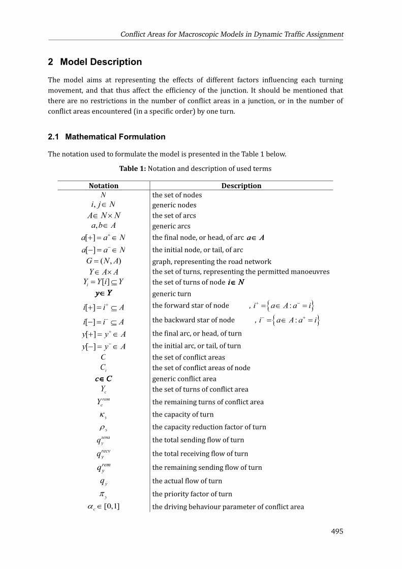
The notation used to formulate the model is presented in the Table 1 below.

Table 1: Notation and description of used terms

Notation Description

N the set of nodes

,i j NÎ generic nodes

A N NÎ ´ the set of arcs

,a b AÎ generic arcs

[ ]a a N++ = Î a AÎ

[ ]a a N-- = Î

a AÎ

( , )G N A= graph, representing the road network

Y A AÎ ´ the set of turns, representing the permitted manoeuvres

[ ]iY Y i Y= Í i NÎ

y YÎ generic turn

[ ]i i A++ = Í the forward star of node

i NÎ

, { }:i a A a i+ -= Î =

[ ]i i A-- = Í the backward star of node

i NÎ

, { }:i a A a i- += Î =

[ ]y y A++ = Î

y YÎ

[ ]y y A-- = Î

y YÎ

C the set of conflict areas

iC the set of conflict areas of

i NÎ

c CÎ generic conflict area

cY

c CÎ

rem

cY

c CÎ

yk the capacity of turn

y YÎ

yr the capacity reduction factor of turn

y YÎ

send

yq

y YÎ

recvyq

y YÎ

remyq

y YÎ

yq the actual flow

y YÎ

yp the priority factor of turn

y YÎ

[0,1]ca Î the driving behaviour parameter of conflict area

c CÎ

Conflict Areas for Macroscopic Models in Dynamic Traffic Assignment

495

Notation Description

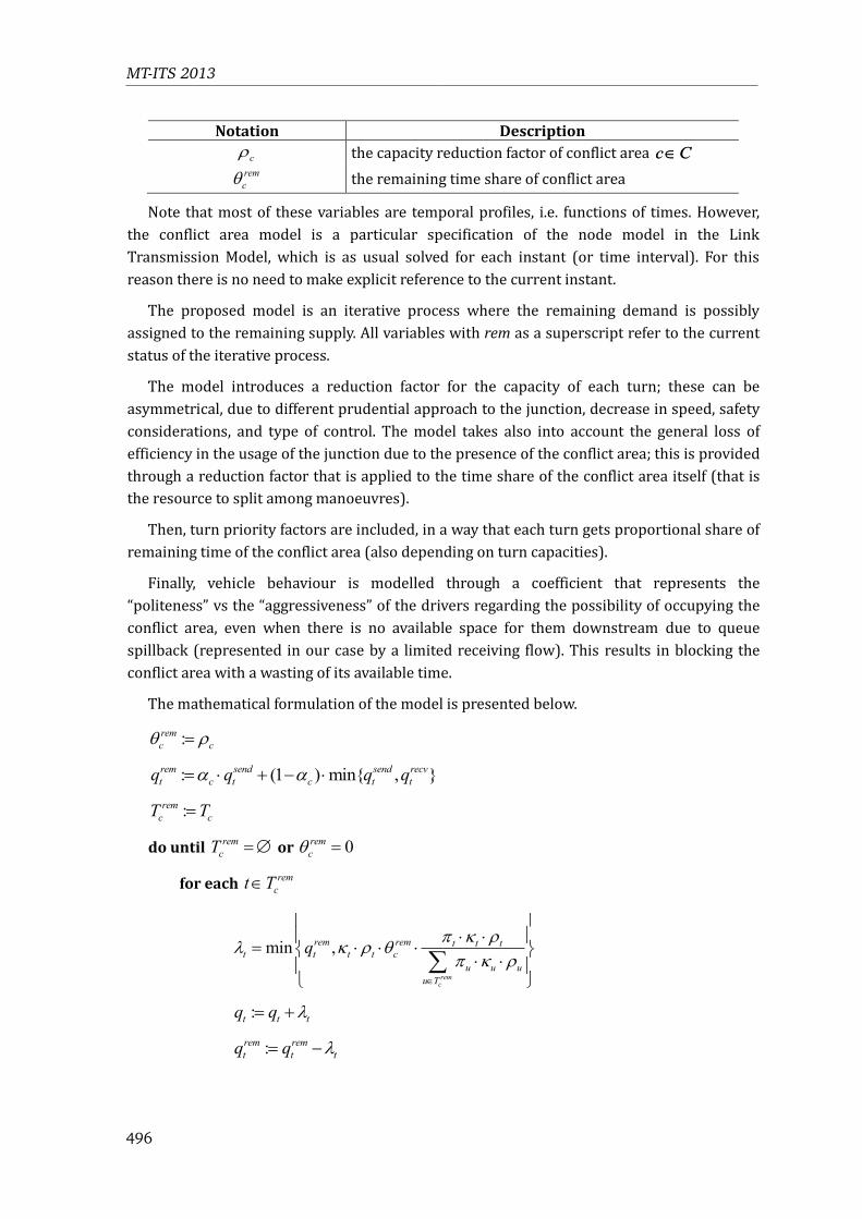
cr the capacity reduction factor of conflict area c CÎ

rem

cq

c CÎ

Note that most of these variables are temporal profiles, i.e. functions of times. However,

the conflict area model is a particular specification of the node model in the Link

Transmission Model, which is as usual solved for each instant (or time interval). For this

reason there is no need to make explicit reference to the current instant.

The proposed model is an iterative process where the remaining demand is possibly

assigned to the remaining supply. All variables with rem as a superscript refer to the current

status of the iterative process.

The model introduces a reduction factor for the capacity of each turn; these can be

asymmetrical, due to different prudential approach to the junction, decrease in speed, safety

considerations, and type of control. The model takes also into account the general loss of

efficiency in the usage of the junction due to the presence of the conflict area; this is provided

through a reduction factor that is applied to the time share of the conflict area itself (that is

the resource to split among manoeuvres).

Then, turn priority factors are included, in a way that each turn gets proportional share of

remaining time of the conflict area (also depending on turn capacities).

Finally, vehicle behaviour is modelled through a coefficient that represents the

“politeness” vs the “aggressiveness” of the drivers regarding the possibility of occupying the

conflict area, even when there is no available space for them downstream due to queue

spillback (represented in our case by a limited receiving flow). This results in blocking the

conflict area with a wasting of its available time.

The mathematical formulation of the model is presented below.

:rem

c cq r=

: (1 ) min{ , }rem send send recv

t c t c t tq q q qa a= × + - ×

:rem

c cT T=

do until rem

cT =Æ or 0rem

cq =

for each rem

ct TÎ

min ,

remc

rem rem t t tt t t t c

u u u

u T

qp k r

l k r qp k r

Î

ì üï ï× ×

= × × ×í ý× ×ï ï

î þå

:t t tq q l= +

:rem rem

t t tq q l= -

MT-ITS 2013

496

:rem rem tc c

t t

lq q

k r= -

×

if 0rem

tq = then : { }rem rem

c cT T t= -

next t

loop

: (1 ) min , ;1recv

tt c c t c t

t

qq t T q q

qa a

ì ü= - × " Î × + ×í ý

î þ

The above procedure can be synthetized in the following Conflict Area Model:

( ), , ; , ; , , , ,CAM send recv

t t u u c c c u u u c cq q q q u T u T t T= " Î " Î " Îa r k r p .

Modelling Conflict Areas in Visum 2.2

To reproduce conflict areas in TRE, they first have to be coded in a data structure. In Visum

this is ensured by creating five user-defined attributes for lane turns:

· CONFLICTAREA. Each conflict area is denoted with a string (in the examples we used

capital letters: A, B…). A conflict area is composed of exclusively two manoeuvres.

Flows of lane turns intersecting in a conflict area are both tagged with that string. In

case a lane turn flow crosses several conflict areas, they are reported in order of

crossing and are comma separated (i.e. A, B).

· PRIORITY. The non-negative priority factor is a parameter of proportionality,

together with turn capacities, to the time share of a conflict area that is reserved to

each conflicting flow.

· REDUCTIONFACTOR. Capacity reduction factor due to prudential approach to the

junction. It acts as a multiplier of the remaining time share of conflict area. It takes

values in the range of [0, 1], meaning that 1 represents no reduction in the remaining

time share, and 0 means that there is no time available.

· CONFLICTAREAREDUCTION. The general loss of efficiency in the usage of the

junction due to the presence of the conflict area.

· DRIVERBEHAVIOUR. Represents the human factor that affects the efficiency of a

junction in case when the sending flow of a turn is constrained by its forward star,

which cause disturbances and can affect the conflicting flow. This is the parameter of a

conflict area, not the turn itself. Therefore, every turn of a conflict area should have

the same value of the parameter. It takes values in the range of [0, 1], where 0

represents “polite” behaviour (no effect of the constrained flow on its conflicting flow)

and 1 is used for “impolite” behaviour (conflicting flow is influenced by minimum

capacity ratio).

Conflict Areas for Macroscopic Models in Dynamic Traffic Assignment

497

Once lane turns are created, they have to be filled in with values for all conflict areas. It is

done in Junction editor/Geometry/Lane turns. If no value is entered in some of the fields, it is

assumed to be 1. If turn belongs to several conflict areas and only one value is entered in the

field, it is assumed value for all the conflict areas. Different values for different conflict areas

are comma separated.

3 Model Analysis

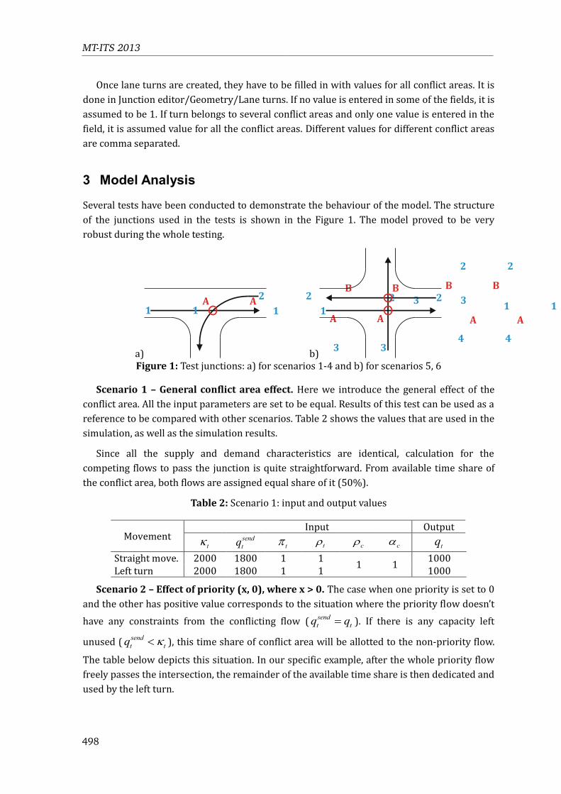
Several tests have been conducted to demonstrate the behaviour of the model. The structure

of the junctions used in the tests is shown in the Figure 1. The model proved to be very

robust during the whole testing.

a) b)

Figure 1: Test junctions: a) for scenarios 1-4 and b) for scenarios 5, 6

Scenario 1 – General conflict area effect. Here we introduce the general effect of the

conflict area. All the input parameters are set to be equal. Results of this test can be used as a

reference to be compared with other scenarios. Table 2 shows the values that are used in the

simulation, as well as the simulation results.

Since all the supply and demand characteristics are identical, calculation for the

competing flows to pass the junction is quite straightforward. From available time share of

the conflict area, both flows are assigned equal share of it (50%).

Table 2: Scenario 1: input and output values

Movement Input Output

tk send

tq tp tr cr ca

tq

Straight move. 2000 1800 1 1 1 1

1000

Left turn 2000 1800 1 1 1000

Scenario 2 – Effect of priority (x, 0), where x > 0. The case when one priority is set to 0

and the other has positive value corresponds to the situation where the priority flow doesn’t

have any constraints from the conflicting flow (send

t tq q= ). If there is any capacity left

unused (send

t tq k< ), this time share of conflict area will be allotted to the non-priority flow.

The table below depicts this situation. In our specific example, after the whole priority flow

freely passes the intersection, the remainder of the available time share is then dedicated and

used by the left turn.

A

B

1

2

3

A1

2

A

13

B

2

4

A

B

1

2

3

A1

2

A

13

B

2

4

MT-ITS 2013

498

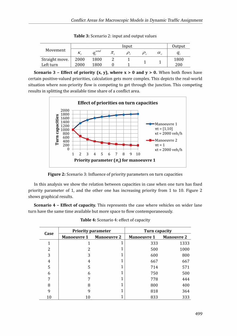
Table 3: Scenario 2: input and output values

Movement Input Output

tk send

tq tp tr cr ca

tq

Straight move. 2000 1800 2 1 1 1

1800

Left turn 2000 1800 0 1 200

Scenario 3 – Effect of priority (x, y), where x > 0 and y > 0. When both flows have

certain positive-valued priorities, calculation gets more complex. This depicts the real-world

situation where non-priority flow is competing to get through the junction. This competing

results in splitting the available time share of a conflict area.

Figure 2: Scenario 3: Influence of priority parameters on turn capacities

In this analysis we show the relation between capacities in case when one turn has fixed

priority parameter of 1, and the other one has increasing priority from 1 to 10. Figure 2

shows graphical results.

Scenario 4 – Effect of capacity. This represents the case where vehicles on wider lane

turn have the same time available but more space to flow contemporaneously.

Table 4: Scenario 4: effect of capacity

Case Priority parameter Turn capacity

Manoeuvre 1 Manoeuvre 2 Manoeuvre 1 Manouvre 2

1 1 1 333 1333

2 2 1 500 1000

3 3 1 600 800

4 4 1 667 667

5 5 1 714 571

6 6 1 750 500

7 7 1 778 444

8 8 1 800 400

9 9 1 818 364

10 10 1 833 333

0200400600800

100012001400160018002000

1 2 3 4 5 6 7 8 9 10

Tu

rn c

ap

ac

itie

s

Priority parameter (πt) for manoeuvre 1

Effect of priorities on turn capacities

Manoeuvre 1

πt = [1,10]

κt = 2000 veh/h

Manoeuvre 2

πt = 1

κt = 2000 veh/h

Conflict Areas for Macroscopic Models in Dynamic Traffic Assignment

499

Here the turn with higher capacity (2000 veh/h) has constant priority parameter of 1. The

conflicting turn has capacity of 1000 veh/h, and raise priority (Table 5).

Scenario 5 – Two conflict areas on one lane turn – the first one constraining. In this

case we test the junction with two conflict areas on one lane turn. The first one is more

constraining than the second one, in order to show how the non-used time share from one

turn is used by the other one.

Conflict area A consists of straight turns 1 and 3, while conflict area B consists of straight

turns 2 and 3 (Figure 1b). Straight turn 3 has lower priority factor in both conflict areas. For

conflict area A, straight movements 1 and 3 get 1333 veh/h and 667 veh/h respectively. In

this case, straight turn 2 gets 900 veh/h, while straight turn 3 gets 800 veh/h. After

calculating the share of unused time (133/2000), this result is multiplied with capacity of the

straight movement 2 and added to the initially calculated capacity, which ultimately gives the

value of 1000 veh/h.

Table 5: Scenario 5: input and output values

Movement Input Output

tk send

tq tp tr cr ca

tq

Straight m. 1 2000 1800 1 1

1 1

1333

Straight m. 2 1500 1800 1 1 1000

Straight m. 3 2000 1800 0.5 1 667

Scenario 6 – Two conflict areas on one lane turn – the second one constraining. In

this case, in contrast to the previous scenario, we put that the second conflict area is the

constraining one, to show the spillback from one conflict area to another. Geometry and

notation are the same as in the previous scenario.

Table 6: Scenario 6: input and output values

Movement Input Output

tk send

tq tp tr cr ca

tq

Straight m. 1 1500 1800 1 1

1 1

750

Straight m. 2 2000 1800 1 1 1333

Straight m. 3 2000 1800 0.5 1 667

Straight movement 3 has lower priority in both conflict areas. Under these circumstances,

conflict area B reduces the capacity of straight movement 3, calculated for conflict area A.

Going back to conflict area A, due to the minimum ratio (because of aggressive driving

behaviour defined by ca ), capacity of straight movement A is reduced accordingly.

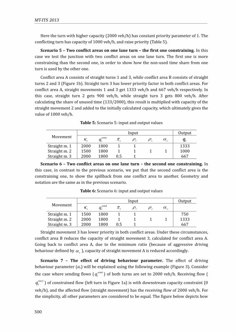
Scenario 7 – The effect of driving behaviour parameter. The effect of driving

behaviour parameter (αc) will be explained using the following example (Figure 3). Consider

the case where sending flows (send

tq ) of both turns are set to 2000 veh/h. Receiving flow (

recvtq ) of constrained flow (left turn in Figure 1a) is with downstream capacity constraint (0

veh/h), and the affected flow (straight movement) has the receiving flow of 2000 veh/h. For

the simplicity, all other parameters are considered to be equal. The figure below depicts how

MT-ITS 2013

500

the flow values, initial remaining flowsremtq and actual turn flows tq , change for different

values of αc. The red line shows that the value of affected flow changes in the non-linear

fashion. Further development of the model should go in the direction of ensuring linear

dependence between driver behaviour parameter and actual flow of the affected turn (black

line).

Figure 3: The effect of driving behaviour parameter (αc)

4 Conclusion

We presented the new Conflict Area Model for modelling and simulation of conflict areas at

junctions. Detailed mathematical model is shown. We introduced several factors that affect

the performance of the junctions and turns. They are capacity reduction factor, due to the

prudential approach to the junction; reduction factor for conflict area due to the general loss

of effectiveness; priority factor, to address the precedence at the junction; and driving

behaviour characteristic, which represents the “politeness” of drivers with respect to

blocking the conflicting flow. Various scenarios are tested and numerical results confirmed

the model to be very robust. Further developments should include corrected effect of the

driving behaviour parameter.

References

[Cor12] R. CORTHOUT: “Intersection modelling and marginal simulation in macroscopic

dynamic network loading”. PhD thesis. Leuven, Belgium: University of Leuven,

2012.

[Gen08] G. GENTILE: “The General Link Transmission Model for dynamic network loading

and a comparison with the DUE algorithm”. In: 2nd International Symposium on

Dynamic Traffic Assignment – DTA 2008. Leuven, Belgium, 2008.

[Gen11] G. GENTILE and L. MESCHINI: “Using dynamic assignment models for real-time traffic

forecast on large urban”. In: 2nd International Conference on Models and Technolo-

0

200

400

600

800

1000

1200

1400

1600

1800

2000

0 0,1 0,2 0,3 0,4 0,5 0,6 0,7 0,8 0,9 1

Flo

w

Driving behaviour parameter (αc)

The effect of driving behaviour parameter (αc)

qtrem for constrained flow

qt for constrained flow

qtrem for affected flow

qt for affected flow

qt desired for affected flow

Conflict Areas for Macroscopic Models in Dynamic Traffic Assignment

501

gies for Intelligent Transportation Systems. Leuven, Belgium, Jun. 22–24, 2011.

[PTV10] PTV AG: VISSIM 5.30 User Manual. Karlsruhe, Germany: PTV AG, 2010.

[PTV12] PTV AG: VISUM 12.5 User Manual. Karlsruhe, Germany: PTV AG, 2012.

[Tid12] D. TIDDI: “Models for dynamic network loading and algorithms for traffic signal

synchronization in congested networks”. PhD thesis. Rome, Italy: Sapienza

University of Rome, 2012.

Corresponding author: Bojan Kostic, Sapienza University of Rome, Department of Civil,

Constructional and Environmental Engineering (DICEA), Via Eudossiana 18, 00184 Rome, Italy,

phone: +39 06 445 85737, e-mail: [email protected]

MT-ITS 2013

502