Confirmatory Factor Analysis with R James H. Steiger Psychology 312 Spring 2013 Traditional Exploratory factor analysis (EFA) is often not purely exploratory in nature. The data analyst brings to the enterprise a substantial amount of intellectual baggage that affects the selection of variables, choice of a number of factors, the naming of factors, and in some cases the way factors are rotated to simple structure. So to some extent, EFA is actually confirmatory in nature. Confirmatory factor analysis (CFA) provides a more explicit framework for confirming prior notions about the structure of a domain of content. CFA adds the ability to test constraints on the parameters of the factor model to the methodology of EFA. In practice, people frequently combine EFA and CFA, to the extent that the appropriate statistical model is not actually determinable. However, we’ll begin with an example of purely confirmatory factor analysis. 1 . “Pure” Confirmatory Factor Analysis Consider the Athletics Data example we examined in conjunction with EFA. Suppose that, prior to analyzing the data, we hypothesized that there were 3 uncorrelated factors called Endurance, Strength, and Hand-Eye Coordination, and that each factor has non- zero loadings on only 3 variables. Such a hypothesis is, of course, extremely unlikely to be true, a point we will return to later. Taken literally, with a suitable ordering of the 9 observed variables, this hypothesis implies that the common factor pattern is of the form

Welcome message from author
This document is posted to help you gain knowledge. Please leave a comment to let me know what you think about it! Share it to your friends and learn new things together.
Transcript

ConfirmatoryFactorAnalysiswithRJamesH.Steiger
Psychology 312
Spring 2013
Traditional Exploratory factor analysis (EFA) is often not purely exploratory in nature.
The data analyst brings to the enterprise a substantial amount of intellectual baggage
that affects the selection of variables, choice of a number of factors, the naming of
factors, and in some cases the way factors are rotated to simple structure. So to some
extent, EFA is actually confirmatory in nature.
Confirmatory factor analysis (CFA) provides a more explicit framework for confirming
prior notions about the structure of a domain of content. CFA adds the ability to test
constraints on the parameters of the factor model to the methodology of EFA.
In practice, people frequently combine EFA and CFA, to the extent that the
appropriate statistical model is not actually determinable. However, we’ll begin with an
example of purely confirmatory factor analysis.
1.“Pure”ConfirmatoryFactorAnalysis
Consider the Athletics Data example we examined in conjunction with EFA. Suppose
that, prior to analyzing the data, we hypothesized that there were 3 uncorrelated factors
called Endurance, Strength, and Hand-Eye Coordination, and that each factor has non-
zero loadings on only 3 variables. Such a hypothesis is, of course, extremely unlikely to
be true, a point we will return to later. Taken literally, with a suitable ordering of the 9
observed variables, this hypothesis implies that the common factor pattern is of the
form
1
2
3
4
5
6
7
8
9
0 0
0 0
0 0
0 0
0 0
0 0
0 0
0 0
0 0
qqq
qqq
qqq
é ùê úê úê úê úê úê úê úê ú
= ê úê úê úê úê úê úê úê úê úê úë û
F
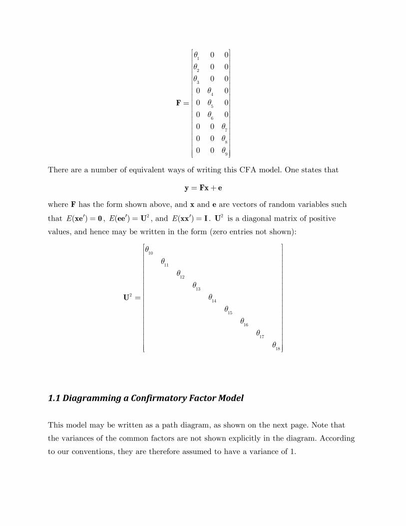
There are a number of equivalent ways of writing this CFA model. One states that
= +y Fx e
where F has the form shown above, and x and e are vectors of random variables such
that ( )E ¢ =xe 0 , 2( )E ¢ =ee U , and ( )E ¢ =xx I . 2U is a diagonal matrix of positive
values, and hence may be written in the form (zero entries not shown):
10
11
12
13
14
15
16
7
8
2
1
1
q
é ùê úê úê úê úê úê úê úê ú
= ê úê úê úê úê úê úê úê úê úê úë û
U
1.1DiagrammingaConfirmatoryFactorModel
This model may be written as a path diagram, as shown on the next page. Note that
the variances of the common factors are not shown explicitly in the diagram. According
to our conventions, they are therefore assumed to have a variance of 1.

Note also that the coefficient from a residual to an observed variable is not labeled in
the diagram, while the coefficient from a common factor to an observed variable is
labeled. For example, the coefficient from 1
x (“Endurance”) to 1
y (“1500 Meter Run”) is
1q . This means that this coefficient is a free parameter that is estimated by the CFA
software. On the other hand, the coefficient from 1e to
1y (“1500 Meter Run”) is not
labeled, and is therefore assumed to be a fixed value of 1.
1q
2q
3q
10q
11q
12q
4q
5q
6q
13q
14q
15q
7q
8q
9q
16q
17q
18q
So the top part of the diagram, shown below, stands for the equation
1 1 1 1y xq e= + ,
where 1
x has a variance of 1 and 1e has a variance of
10q .

1q
10q
Recall that, in any path diagram, variables are either manifest or latent, and either
exogenous or endogenous. Here are some questions for you. See if you can answer them,
then check your answers in the footnote1 below. What kind of variable is “Endurance”
in the preceding diagram? What kind of variable is “1500 Meter Run”? What kind of
variable is “1e ”?
A number of programs are available to fit confirmatory factor analysis models to data.
Some of these programs are free. One such program is available as the R package sem.
Another is the program Mx.
Our diagramming system transparently connects with the standard linear equations
coding of a structural equation model. Each and every linear equation has a
corresponding element in the diagram. Moreover, each path in the diagram can be coded
unambiguously in an ASCII computer language called PATH1 (Steiger, 1988).
1.2ThesemprogramandtheRAMDiagrammingSystem
The sem package has the capability of decoding a language and diagramming system
that follows our general rules for path diagrams (except that it requires latent variable
variances of 1 to be represented explicitly). However, it is better designed
computationally to handle a slightly abbreviated diagramming system that makes a
couple of exceptions to these rules. This latter diagramming system, which I will call
RAM, does not maintain a direct visual correspondence with the underlying linear
equation system. When we discuss the major algebraic approaches to path models (the
LISREL, RAM1, RAM2, Bentler-Weeks, and EzPath models), we will discuss the
1 “Endurance” is latent-exogenous, “1500 Meter Run” is manifest-endogenous, and “e1” is latent-
exogenous.
distinction between the original (RAM1) specification of J. J. McArdle, and the
improved RAM2 model specification that sem is designed around.
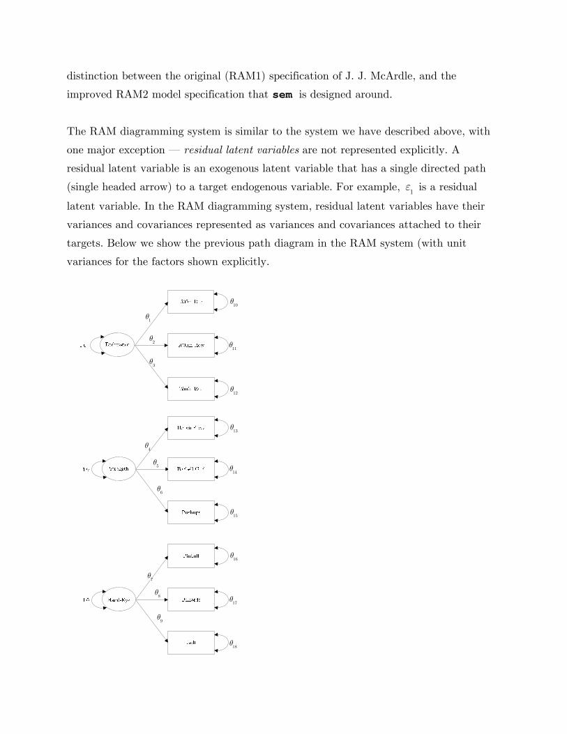
The RAM diagramming system is similar to the system we have described above, with
one major exception — residual latent variables are not represented explicitly. A
residual latent variable is an exogenous latent variable that has a single directed path
(single headed arrow) to a target endogenous variable. For example, 1e is a residual
latent variable. In the RAM diagramming system, residual latent variables have their
variances and covariances represented as variances and covariances attached to their
targets. Below we show the previous path diagram in the RAM system (with unit
variances for the factors shown explicitly.
1q
2q
3q
12q
4q
5q
6q
13q
14q
15q
7q
8q
9q
16q
17q
18q
10q
11q

The two-headed arrows, or “slings,” mean something different on the left side of the
diagram than they do on the right side of the diagram. On the left side, they stand for
the variances of the latent variables, while on right side, they are the variances of the
(hidden) residual variables. This system is visually more compact in its use of space
than the system described earlier, because some objects are not represented explicitly.
On the other hand, this system requires more effort to decode, because (a) there are
more arrowheads, and (b) the meaning of a two-headed arrow varies, depending on the
status of the target variable it is attached to, which in turn has to be determined by
examining whether the target variable is endogenous or exogenous. This double usage
of the two-headed arrow also rules out other possible usages in a more complex system.
For example, some systems allow unit variance constraints to be placed on the variances
of endogenous latent variables, and these constraints are indicated in the path diagram
with a two-headed arrow attached to the endogenous latent variable. (The residual
variance is indicated with an explicit residual variable.) This system cannot be
employed in conjunction with the RAM system.
The sem package can decode a model represented in the RAM path diagramming
system rather easily. For each sling or arrow, the user includes a line in a rather natural
ASCII language. Each line is of the form
<Relation>, <Parameter Symbol>, <Parameter Value>
<Relation> indicates the arrow or sling. Arrows are represented in the form
name1 -> name2
Slings (two-headed arrows) are represented as
name1 <-> name2
The <Parameter Symbol> is a label used to uniquely identify a free parameter. If the
parameter symbol is NA, the path has a fixed value. If two paths have the same free

parameter label, the numerical value for that parameter is constrained to be the same
for both paths.
The <Parameter Value> is the starting value for iteration if the parameter is free (a
value of NA will cause the program to use an automatic starting value), the fixed
numerical value if the parameter symbol is NA and the value is fixed.
To see how this system works, compare the code on the following page with the path
diagram. Note that you must use the variable names in the data file. I’ve included some
comment lines to set off key areas of the code.
## Factor 1 -- Endurance Endurance -> X.1500M, theta01, NA Endurance -> X.2KROW, theta02, NA Endurance -> X.12MINTR,theta03, NA ## Factor 2 -- Strength Strength -> BENCH, theta04, NA Strength -> CURL, theta05, NA Strength -> MAXPUSHU, theta06, NA ## Factor 3 -- Hand-Eye Coordination Hand-Eye -> PINBALL, theta07, NA Hand-Eye -> BILLIARD, theta08, NA Hand-Eye -> GOLF, theta09, NA ## Unique Variances X.1500M <-> X.1500M, theta10, NA X.2KROW <-> X.2KROW, theta11, NA X.12MINTR <-> X.12MINTR, theta12, NA BENCH <-> BENCH, theta13, NA CURL <-> CURL, theta14, NA MAXPUSHU <-> MAXPUSHU, theta15, NA PINBALL <-> PINBALL, theta16, NA BILLIARD <-> BILLIARD, theta17, NA GOLF <-> GOLF, theta18, NA ## Factor Variances fixed at 1 Endurance <-> Endurance, NA, 1 Strength <-> Strength, NA, 1 Hand-Eye <-> Hand-Eye, NA, 1
Suppose we save the above code into an ASCII file called CFA1.r (say, with NotePad).
After loading the Hmisc library, loading the AthleticsData file and attaching it with the
following 3 lines, we are ready to go.
> library(Hmisc) > AthleticsData <- spss.get("AthleticsData.sav") > attach(AthleticsData)
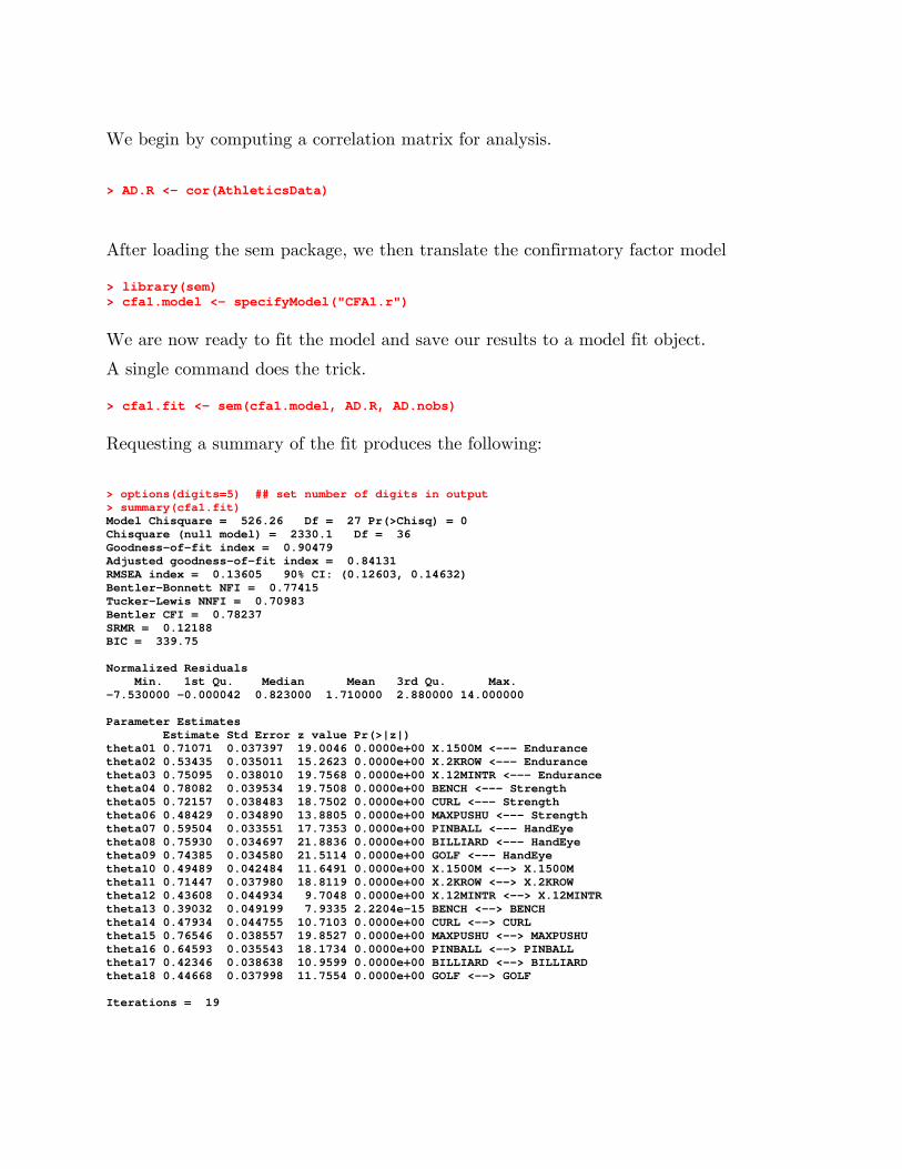
We begin by computing a correlation matrix for analysis.
> AD.R <- cor(AthleticsData)
After loading the sem package, we then translate the confirmatory factor model > library(sem) > cfa1.model <- specifyModel("CFA1.r")
We are now ready to fit the model and save our results to a model fit object.
A single command does the trick. > cfa1.fit <- sem(cfa1.model, AD.R, AD.nobs)
Requesting a summary of the fit produces the following:
> options(digits=5) ## set number of digits in output > summary(cfa1.fit) Model Chisquare = 526.26 Df = 27 Pr(>Chisq) = 0 Chisquare (null model) = 2330.1 Df = 36 Goodness-of-fit index = 0.90479 Adjusted goodness-of-fit index = 0.84131 RMSEA index = 0.13605 90% CI: (0.12603, 0.14632) Bentler-Bonnett NFI = 0.77415 Tucker-Lewis NNFI = 0.70983 Bentler CFI = 0.78237 SRMR = 0.12188 BIC = 339.75 Normalized Residuals Min. 1st Qu. Median Mean 3rd Qu. Max. -7.530000 -0.000042 0.823000 1.710000 2.880000 14.000000 Parameter Estimates Estimate Std Error z value Pr(>|z|) theta01 0.71071 0.037397 19.0046 0.0000e+00 X.1500M <--- Endurance theta02 0.53435 0.035011 15.2623 0.0000e+00 X.2KROW <--- Endurance theta03 0.75095 0.038010 19.7568 0.0000e+00 X.12MINTR <--- Endurance theta04 0.78082 0.039534 19.7508 0.0000e+00 BENCH <--- Strength theta05 0.72157 0.038483 18.7502 0.0000e+00 CURL <--- Strength theta06 0.48429 0.034890 13.8805 0.0000e+00 MAXPUSHU <--- Strength theta07 0.59504 0.033551 17.7353 0.0000e+00 PINBALL <--- HandEye theta08 0.75930 0.034697 21.8836 0.0000e+00 BILLIARD <--- HandEye theta09 0.74385 0.034580 21.5114 0.0000e+00 GOLF <--- HandEye theta10 0.49489 0.042484 11.6491 0.0000e+00 X.1500M <--> X.1500M theta11 0.71447 0.037980 18.8119 0.0000e+00 X.2KROW <--> X.2KROW theta12 0.43608 0.044934 9.7048 0.0000e+00 X.12MINTR <--> X.12MINTR theta13 0.39032 0.049199 7.9335 2.2204e-15 BENCH <--> BENCH theta14 0.47934 0.044755 10.7103 0.0000e+00 CURL <--> CURL theta15 0.76546 0.038557 19.8527 0.0000e+00 MAXPUSHU <--> MAXPUSHU theta16 0.64593 0.035543 18.1734 0.0000e+00 PINBALL <--> PINBALL theta17 0.42346 0.038638 10.9599 0.0000e+00 BILLIARD <--> BILLIARD theta18 0.44668 0.037998 11.7554 0.0000e+00 GOLF <--> GOLF Iterations = 19

The above output shows that the solution converged in 19 iterations, yielding a model 2c statistic of 526.26 with 27 degrees of freedom. Where did this “degrees of freedom”
value come from? In general, it is the number of non-redundant elements of the
covariance p p´ matrix minus the number of free parameters. In this case, the
covariance matrix is 9 9´ , so there are ( 1)/ 2 9(9 1)/ 2 45p p + = + = non-redundant
elements. Since there are 18 free parameters (1q through
18q ), there are 45 18 27- =
degrees of freedom.
This 2c value, of course, has a p-value far below .001, and so the null hypothesis of
perfect fit is rejected. The output also includes parameter values, estimates of their
standard errors, and asymptotically normal statistics testing the hypothesis that the
parameter value is zero in the population. One can also construct an approximate 95%
confidence interval by taking the estimate plus or minus two standard errors.
1.3EvaluatingandImprovingModelFit
The fact that the hypothesis of perfect fit is rejected is, in itself, not very informative —
the common factor model is highly constrained, and with a sample size of 1000, we have
excellent power to detect even minor levels of misfit. The more important statistical
questions are, (a) how bad is the misfit, and (b) how precisely have we have we
determined the degree of misfit. For a detailed account of several of these indices and
their theoretical basis, see the course handout on “Indices of Fit in Structural Equation
Modeling.”
The fact that the RMSEA confidence interval ranges from .126 to .146 suggests to many
people that the model fit, in this case, can definitely be improved. Of course, we know
from the earlier exploratory factor analysis of these same data that there are two
moderately high “crossover loadings” that are not included in the model we just
evaluated, so this model is definitely missing some key elements. However, suppose we
did not know that? How would we proceed?

The “pure” confirmatory approach would suggest that we not proceed at all! We had a
model, it doesn’t fit, and “well — that’s it.” Of course, in general people do proceed,
sometimes at the peril of objective scientific values. Below, we sketch two popular
approaches to arriving at a confirmatory factor model through a mixture of exploratory
and confirmatory approaches.
2.The“ConfirmandUpdate”Approach
One approach, introduced by Jöreskog, is to start with a confirmatory model based on
theory, then update it by adding factor loadings with the aid of “modification indices.”
These indices attempt to estimate which missing paths, if added to the current model,
would result in the greatest reduction of the 2c fit statistic.
Obtaining modification indices from sem is straightforward. > modIndices(cfa1.fit) 5 largest modification indices, A matrix: MAXPUSHU<-Endurance X.2KROW<-Strength MAXPUSHU<-X.1500M MAXPUSHU<-X.2KROW 186.74 170.23 147.17 132.17 Endurance<-MAXPUSHU 128.88 5 largest modification indices, P matrix: Endurance<->MAXPUSHU Strength<->X.2KROW BENCH<->X.1500M Strength<->X.1500M 186.742 170.232 63.265 59.284 Endurance<->BENCH 44.768
Interpreting the above is facilitated by a knowledge of the RAM1 model of McArdle and
McDonald. However, essentially it works like this. An entry in the A matrix is of the
form, <endogenous variable>:<exogenous variable>. So, the largest
modification index, labeled MAXPUSHU:Endurance, indicates that the model 2c fit
index would be decreased by roughly 187 if a path from Endurance to MAXPUSHU were
added to the model. Let’s try it, by simply adding a single line to the previous model
and, for documentation purposes, saving the revised model to a new file called CFA2.r.
This line is “Endurance -> MAXPUSHU, theta19, NA”.

We fit the model, > cfa2.model <- specifyModel("CFA2.r")
Note: An alternative method for updating the model is to add a path using the update
method. Here is an example:
> cfa2.model <- update(cfa1.model) > add, Endurance -> MAXPUSHU, theta19, NA
After terminating the sequence by hitting the <Enter> key, the new model will be
defined. I prefer to have a separate file for each model, but this method may actually
be faster. After entering the new lines, enter a blank line to terminate the update
input.
Run the new model > cfa2.fit <- sem(cfa2.model, AD.R, AD.nobs)
then examine the results.
> summary(cfa2.fit) Model Chisquare = 310.32 Df = 26 Pr(>Chisq) = 0 Chisquare (null model) = 2330.1 Df = 36 Goodness-of-fit index = 0.93856 Adjusted goodness-of-fit index = 0.89367 RMSEA index = 0.10463 90% CI: (0.094363, 0.11522) Bentler-Bonnett NFI = 0.86682 Tucker-Lewis NNFI = 0.8284 Bentler CFI = 0.87607 SRMR = 0.093325 BIC = 130.72 Normalized Residuals Min. 1st Qu. Median Mean 3rd Qu. Max. -7.530 -0.323 0.444 0.910 2.410 7.520 Parameter Estimates Estimate Std Error z value Pr(>|z|) theta01 0.73778 0.033684 21.9032 0.0000e+00 X.1500M <--- Endurance theta02 0.56030 0.034651 16.1699 0.0000e+00 X.2KROW <--- Endurance theta03 0.70195 0.033341 21.0540 0.0000e+00 X.12MINTR <--- Endurance theta04 0.81307 0.036707 22.1502 0.0000e+00 BENCH <--- Strength theta05 0.69295 0.035394 19.5781 0.0000e+00 CURL <--- Strength theta06 0.52020 0.032383 16.0638 0.0000e+00 MAXPUSHU <--- Strength theta07 0.59503 0.033551 17.7352 0.0000e+00 PINBALL <--- HandEye theta08 0.75931 0.034697 21.8837 0.0000e+00 BILLIARD <--- HandEye theta09 0.74385 0.034580 21.5112 0.0000e+00 GOLF <--- HandEye theta10 0.45568 0.036057 12.6376 0.0000e+00 X.1500M <--> X.1500M

theta11 0.68607 0.037295 18.3959 0.0000e+00 X.2KROW <--> X.2KROW theta12 0.50726 0.034922 14.5257 0.0000e+00 X.12MINTR <--> X.12MINTR theta13 0.33892 0.044964 7.5376 4.7962e-14 BENCH <--> BENCH theta14 0.51982 0.038556 13.4824 0.0000e+00 CURL <--> CURL theta15 0.53297 0.033166 16.0700 0.0000e+00 MAXPUSHU <--> MAXPUSHU theta16 0.64594 0.035543 18.1734 0.0000e+00 PINBALL <--> PINBALL theta17 0.42345 0.038638 10.9594 0.0000e+00 BILLIARD <--> BILLIARD theta18 0.44669 0.037998 11.7556 0.0000e+00 GOLF <--> GOLF theta19 0.47879 0.031654 15.1260 0.0000e+00 MAXPUSHU <--- Endurance Iterations = 19
We see that the new parameter, 19q , has an estimate value of .48, and is highly
significant. Moreover, the model 2c statistic decreased to 310, a 215 point decrease even
greater than the modification index predicted. According to statistical theory in Steiger,
Shapiro, and Browne (1984), since the models are nested (The first model is a special
case of the second, where one of the parameters is constrained to zero), you can treat
the difference in the two 2c values as a 2c with degrees of freedom equal to the
difference in their degrees of freedom (i. e., 1 in this case). The resulting chi square
difference statistic provides a method for testing whether there is a statistically different
improvement in fit. Clearly there is!
However, the RMSEA statistic for the improved model is still larger (.10) than the
recommended value. We recompute the modification indices:
> modIndices(cfa2.fit)
5 largest modification indices, A matrix: X.2KROW:Strength X.2KROW:BENCH X.2KROW:CURL X.1500M:BENCH 164.62477 137.49080 103.45883 89.50040 X.1500M:Strength 84.81637
The largest modification index is for a path from Strength to X.2KROW. Adding this
path to the model with the line “Strength -> X.2KROW, theta20, NA” and
saving the new model to CFA3.r (or updating as described above), we refit the model
again,
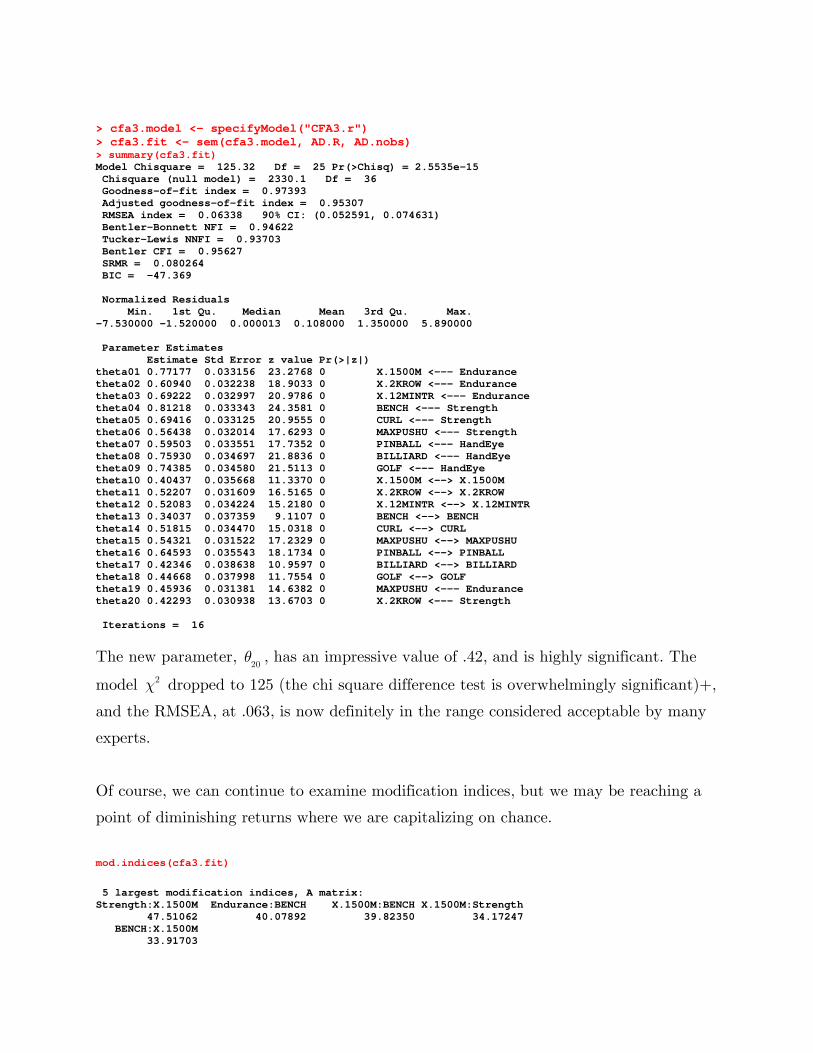
> cfa3.model <- specifyModel("CFA3.r") > cfa3.fit <- sem(cfa3.model, AD.R, AD.nobs) > summary(cfa3.fit) Model Chisquare = 125.32 Df = 25 Pr(>Chisq) = 2.5535e-15 Chisquare (null model) = 2330.1 Df = 36 Goodness-of-fit index = 0.97393 Adjusted goodness-of-fit index = 0.95307 RMSEA index = 0.06338 90% CI: (0.052591, 0.074631) Bentler-Bonnett NFI = 0.94622 Tucker-Lewis NNFI = 0.93703 Bentler CFI = 0.95627 SRMR = 0.080264 BIC = -47.369 Normalized Residuals Min. 1st Qu. Median Mean 3rd Qu. Max. -7.530000 -1.520000 0.000013 0.108000 1.350000 5.890000 Parameter Estimates Estimate Std Error z value Pr(>|z|) theta01 0.77177 0.033156 23.2768 0 X.1500M <--- Endurance theta02 0.60940 0.032238 18.9033 0 X.2KROW <--- Endurance theta03 0.69222 0.032997 20.9786 0 X.12MINTR <--- Endurance theta04 0.81218 0.033343 24.3581 0 BENCH <--- Strength theta05 0.69416 0.033125 20.9555 0 CURL <--- Strength theta06 0.56438 0.032014 17.6293 0 MAXPUSHU <--- Strength theta07 0.59503 0.033551 17.7352 0 PINBALL <--- HandEye theta08 0.75930 0.034697 21.8836 0 BILLIARD <--- HandEye theta09 0.74385 0.034580 21.5113 0 GOLF <--- HandEye theta10 0.40437 0.035668 11.3370 0 X.1500M <--> X.1500M theta11 0.52207 0.031609 16.5165 0 X.2KROW <--> X.2KROW theta12 0.52083 0.034224 15.2180 0 X.12MINTR <--> X.12MINTR theta13 0.34037 0.037359 9.1107 0 BENCH <--> BENCH theta14 0.51815 0.034470 15.0318 0 CURL <--> CURL theta15 0.54321 0.031522 17.2329 0 MAXPUSHU <--> MAXPUSHU theta16 0.64593 0.035543 18.1734 0 PINBALL <--> PINBALL theta17 0.42346 0.038638 10.9597 0 BILLIARD <--> BILLIARD theta18 0.44668 0.037998 11.7554 0 GOLF <--> GOLF theta19 0.45936 0.031381 14.6382 0 MAXPUSHU <--- Endurance theta20 0.42293 0.030938 13.6703 0 X.2KROW <--- Strength Iterations = 16
The new parameter, 20q , has an impressive value of .42, and is highly significant. The
model 2c dropped to 125 (the chi square difference test is overwhelmingly significant)+,
and the RMSEA, at .063, is now definitely in the range considered acceptable by many
experts.
Of course, we can continue to examine modification indices, but we may be reaching a
point of diminishing returns where we are capitalizing on chance.
mod.indices(cfa3.fit)
5 largest modification indices, A matrix: Strength:X.1500M Endurance:BENCH X.1500M:BENCH X.1500M:Strength 47.51062 40.07892 39.82350 34.17247 BENCH:X.1500M 33.91703

5 largest modification indices, P matrix: Strength:X.1500M Strength:Endurance HandEye:Strength Endurance:BENCH 34.17247 32.66084 26.38424 24.81201 BENCH:X.1500M 22.04953
Notice how all the modification indices are rather close, and are now much smaller than
before. Remember that the first variable in the A matrix is the variable the arrow goes
to, so we are looking only at paths from a latent variable to a manifest variable. Let’s
add a path from Strength to X.1500M and see what happens.
> cfa4.model <- specifyModel("CFA4.r") > cfa4.fit <- sem(cfa4.model, AD.R, AD.nobs) > summary(cfa4.fit) Model Chisquare = 81.641 Df = 24 Pr(>Chisq) = 3.3251e-08 Chisquare (null model) = 2330.1 Df = 36 Goodness-of-fit index = 0.983 Adjusted goodness-of-fit index = 0.96812 RMSEA index = 0.049032 90% CI: (0.037601, 0.060921) Bentler-Bonnett NFI = 0.96496 Tucker-Lewis NNFI = 0.96231 Bentler CFI = 0.97487 SRMR = 0.061516 BIC = -84.145 Normalized Residuals Min. 1st Qu. Median Mean 3rd Qu. Max. -3.3500 -0.3240 0.0666 0.6760 1.3800 5.8900 Parameter Estimates Estimate Std Error z value Pr(>|z|) theta01 0.76727 0.032380 23.6957 0.0000e+00 X.1500M <--- Endurance theta02 0.61213 0.031840 19.2251 0.0000e+00 X.2KROW <--- Endurance theta03 0.67383 0.032764 20.5664 0.0000e+00 X.12MINTR <--- Endurance theta04 0.82465 0.032818 25.1282 0.0000e+00 BENCH <--- Strength theta05 0.68468 0.032785 20.8841 0.0000e+00 CURL <--- Strength theta06 0.50656 0.032462 15.6048 0.0000e+00 MAXPUSHU <--- Strength theta07 0.59503 0.033551 17.7352 0.0000e+00 PINBALL <--- HandEye theta08 0.75930 0.034697 21.8836 0.0000e+00 BILLIARD <--- HandEye theta09 0.74385 0.034580 21.5113 0.0000e+00 GOLF <--- HandEye theta10 0.35235 0.035665 9.8796 0.0000e+00 X.1500M <--> X.1500M theta11 0.52539 0.031764 16.5406 0.0000e+00 X.2KROW <--> X.2KROW theta12 0.54595 0.033784 16.1600 0.0000e+00 X.12MINTR <--> X.12MINTR theta13 0.31995 0.036578 8.7470 0.0000e+00 BENCH <--> BENCH theta14 0.53121 0.033818 15.7081 0.0000e+00 CURL <--> CURL theta15 0.54467 0.031649 17.2100 0.0000e+00 MAXPUSHU <--> MAXPUSHU theta16 0.64593 0.035543 18.1734 0.0000e+00 PINBALL <--> PINBALL theta17 0.42346 0.038638 10.9596 0.0000e+00 BILLIARD <--> BILLIARD theta18 0.44669 0.037998 11.7555 0.0000e+00 GOLF <--> GOLF theta19 0.47520 0.030764 15.4466 0.0000e+00 MAXPUSHU <--- Endurance theta20 0.35239 0.032025 11.0035 0.0000e+00 X.2KROW <--- Strength theta21 -0.20340 0.030502 -6.6685 2.5845e-11 X.1500M <--- Strength Iterations = 18
We can see that the added parameter has a value of –.20, and the RMSEA has
decreased appreciably to .049, a value generally considered to represent excellent fit.

This latest coefficient seems to imply that increased strength actually hurts performance
in the 1500 meter run!
In practical circumstances, there is no way of determining which model is “correct.”
Indeed, one might argue that it is extremely unlikely that factor loadings (other than a
certain small number of loadings that can always be forced to zero by rotation, as we
will discuss later) are truly zero. On the other hand, “minor loadings” contribute little
to the ability of the factor model to fit data, and, because of sampling error, including
them in the model may be contributing nearly as much noise as signal.
In the above example, we started with a strong “confirmatory” position, based on a
prior understanding about the state of the world, i.e., there are 3 factors, and each
factor has 3 indicator variables. We used modification indices to “upgrade” the model,
and quickly ended up with a model that is parsimonious, seems to “make sense,” and
fits well.
Note that we can continue this process, by recomputing modification indices and
upgrading the model still further. Ultimately however, we have to worry seriously about
the extent to which we are capitalizing on chance.
3.The“Exploratory‐Confirmatory”Approach
An alternative approach, which begins with a purely exploratory factor analysis, was
described by Karl Jöreskog in his 1978 Presidential Address to the Psychometric
Society.
Jöreskog’s approach is as follows:
Perform an exploratory factor analysis, and decide on the number of factors, m.
In many textbook examples, the decision is relatively clear cut. Be forewarned —
in practice the decision may be quite difficult.

Fit an m-factor model, and rotate to simple structure using varimax or promax.
(In the original article, Jöreskog said to use promax, but used varimax in his
numerical example. We’ll use varimax.)
For each column of the factor pattern, find the largest loading, then constrain all
the other loadings in that row to be zero, and fit the resulting model as a
confirmatory factor model. This confirmatory model will have exactly the same
discrepancy function and 2c value as the exploratory factor analysis that
preceded it.
Examine the factor pattern, and test all factor loadings. Delete “non-significant”
loadings from the model. After checking the fit, the user can decide whether to
terminate the process, or look for more loadings to delete.
A detailed commentary on the final steps may prove helpful. Due to the well-known fact
of rotational indeterminacy, the parameters in the exploratory factor model (where
every factor loading is free to vary) are not uniquely determined. In the broader
language of structural equation modeling, we say that the parameters are not
“identified.”
A parameter is a fixed numerical value. To estimate a “parameter,” it obviously follows
that the parameter has to be identified! So in general, a model must be identified in
some way before iteration to a best-fitting solution can be attempted. Therefore, a
model with parameters that are not identified can propose a severe problem for general
structural equation modeling programs like sem.
Exploratory factor analysis programs achieve identification automatically during
iteration by a variety of means, so while doing exploratory factor analysis with a
program designed to do exploratory factor analysis, you don’t need to worry about it.
However, when doing a “completely unrestricted” confirmatory factor analysis with 2 or
more factors, you cannot simply start by letting all the possible p m´ factor loadings be
free parameters. You’d discover that the solution is not identified. Depending on the
sophistication of your program, you’d either converge to a solution and get an error
indicator, or you’d fail to converge with a cryptic error message. sem, unfortunately,
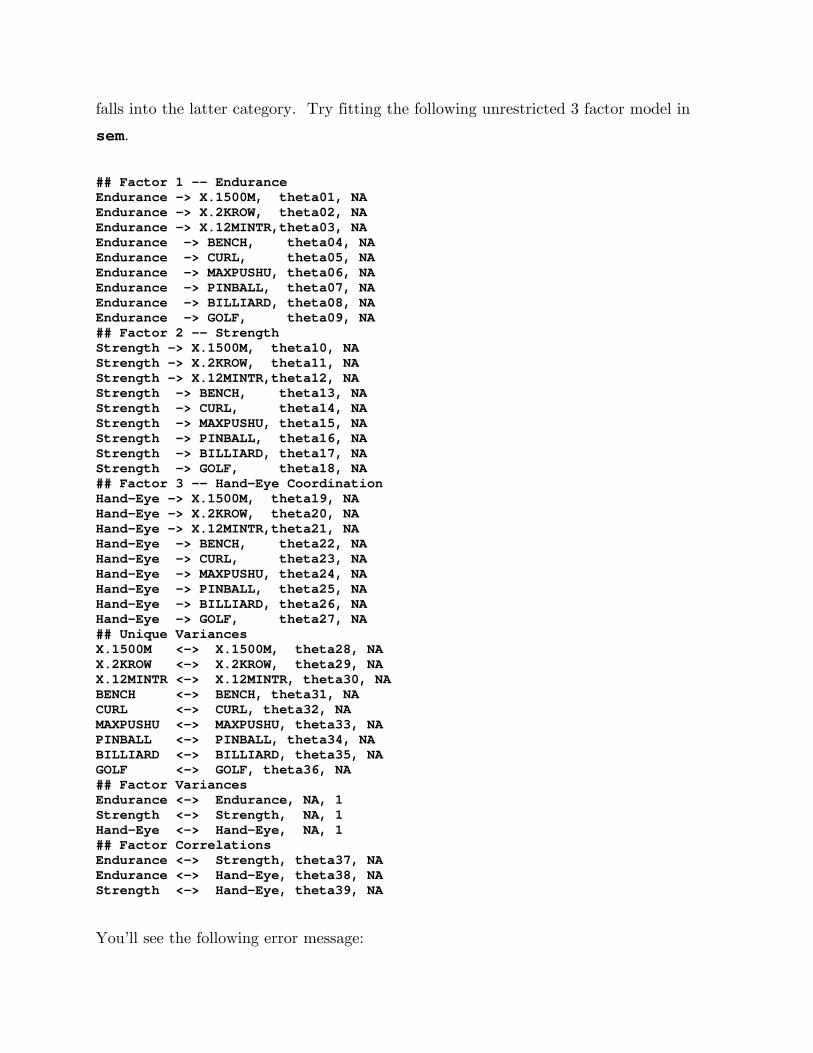
falls into the latter category. Try fitting the following unrestricted 3 factor model in
sem.
## Factor 1 -- Endurance Endurance -> X.1500M, theta01, NA Endurance -> X.2KROW, theta02, NA Endurance -> X.12MINTR,theta03, NA Endurance -> BENCH, theta04, NA Endurance -> CURL, theta05, NA Endurance -> MAXPUSHU, theta06, NA Endurance -> PINBALL, theta07, NA Endurance -> BILLIARD, theta08, NA Endurance -> GOLF, theta09, NA ## Factor 2 -- Strength Strength -> X.1500M, theta10, NA Strength -> X.2KROW, theta11, NA Strength -> X.12MINTR,theta12, NA Strength -> BENCH, theta13, NA Strength -> CURL, theta14, NA Strength -> MAXPUSHU, theta15, NA Strength -> PINBALL, theta16, NA Strength -> BILLIARD, theta17, NA Strength -> GOLF, theta18, NA ## Factor 3 -- Hand-Eye Coordination Hand-Eye -> X.1500M, theta19, NA Hand-Eye -> X.2KROW, theta20, NA Hand-Eye -> X.12MINTR,theta21, NA Hand-Eye -> BENCH, theta22, NA Hand-Eye -> CURL, theta23, NA Hand-Eye -> MAXPUSHU, theta24, NA Hand-Eye -> PINBALL, theta25, NA Hand-Eye -> BILLIARD, theta26, NA Hand-Eye -> GOLF, theta27, NA ## Unique Variances X.1500M <-> X.1500M, theta28, NA X.2KROW <-> X.2KROW, theta29, NA X.12MINTR <-> X.12MINTR, theta30, NA BENCH <-> BENCH, theta31, NA CURL <-> CURL, theta32, NA MAXPUSHU <-> MAXPUSHU, theta33, NA PINBALL <-> PINBALL, theta34, NA BILLIARD <-> BILLIARD, theta35, NA GOLF <-> GOLF, theta36, NA ## Factor Variances Endurance <-> Endurance, NA, 1 Strength <-> Strength, NA, 1 Hand-Eye <-> Hand-Eye, NA, 1 ## Factor Correlations Endurance <-> Strength, theta37, NA Endurance <-> Hand-Eye, theta38, NA Strength <-> Hand-Eye, theta39, NA
You’ll see the following error message:

Error in solve.default(C[ind, ind]) : Lapack routine dgesv: system is exactly singular
With the advantage of a substantial amount of experience, you might be able to
interpret this message as follows:
During iteration, the program tries to invert a matrix that is a scalar multiple of
an estimated variance-covariance matrix of the parameter estimates.
If some parameters are functionally related to others, this estimated asymptotic
covariance matrix will be singular
The system is not “identified,” because some parameters are not needed — they
are determinate functions of other parameters
According to Jöreskog (1978), you can identify a common factor model by setting at
least 1k - loadings in each column of the factor pattern to zero. He provides a scheme
for doing this automatically, based on examination of the pattern after rotating to
simple structure. Jöreskog’s explanation of this step was somewhat terse, and he does
not describe in detail why the system works. In looking carefully at the algebra, we’ll
discover that some of the “free parameters” in a common factor pattern are not “really
free” as you might expect. In other words, if you set up a confirmatory factor model
with all p variables loading on all m factors, and all m factors allowed to correlate with
each other, you will have pm factor loadings and p unique variances, plus ( 1)/ 2m m -
nonredundant factor intercorrelations, yet the “true number of free parameters” is not
really ( 1) / 2pm p m m+ + - . Why not?
The answer stems from the following facts. First, suppose the orthogonal factor model
fits, and
= +y Fx e
with F a p m´ factor pattern of full column rank, with the standard restrictions in
place. First of all, recall the fact of rotational indeterminacy, and assume the factors are
allowed to be correlated after rotation by a matrix T. Then if = +y Fx e , it must also
be true that -1= +y FTT x e for any nonsingular matrix T, so the common factor model

must still fit with new pattern * =F FT and new factors 1* -=x T x with covariance
matrix 1 1- - ¢T T . In general, we wish to retain the restriction that the common factors
have unit variance after rotation by 1-T . So we impose the restriction on 1-T that
1 1diag( ) diag( )- - ¢ =T T I .
Now, suppose that we isolate an m m´ submatrix of F. Note that by suitable
permutation of the (arbitrary) ordering of the variables in y, we can always manipulate
this submatrix into the upper m rows of F. So we can write F in partitioned form as
1
2
é ùê ú= ê úê úë û
FF
F
Suppose that 1
F is nonsingular, and let 1 1
1
- -=T F D , where D is a positive definite
diagonal scaling matrix. Then
1
1 1*1 1
2 2 2 1
-
- -
é ùé ù é ùê úê ú ê ú= = = = ê úê ú ê úê úê ú ê úë û ë û ë û
F FT DF FT T
F FT F F D
Note that the upper m m´ submatrix of *F is diagonal, and contains 2 ( 1)m m m m- = - zeroes. In other words, it is inevitable that any factor pattern can
be rotated obliquely to include that many zeroes. Notice that rotation to this position
has absolutely no effect on how well the model fits. So instead of “really” having pm
free factor loadings, we have ( 1)pm m m- - loadings that are actually free to be
nonzero.
In the previous formula, we did not specify how to calculate the scaling matrix D.
However, it is determined by the restriction that the rotated factors still have unit
variance. This requirement means that 1 1diag( ) diag( )- - ¢ =T T I . Since
1 1
1 1diag( ) diag( )- - ¢ ¢=T T DFF D , it is clear that we can force the latter matrix to have
ones on its diagonal by simply setting 1/2
1 1diag ( )- ¢=D FF , or, equivalently
1 1
1 1
1 1/2
1 1diag ( )- -- ¢= =T F D F FF (1)

Since T operates on the rows of F independently, we do not need to rearrange the rows
of F to manipulate desired rows into the upper m m´ submatrix. Rather, we simply
construct 1
F from the desired rows and apply Equation 1.
A purely hypothetical example constructed using R should help make the above ideas
clear. Suppose we have a factor analysis based on 6 variables and two factors. We
observe the following factor pattern:
> F <- matrix(c(.6,.5,.58,.2,.1,.05,.09,.11,.07,.71,.62,.66),6,2) > F [,1] [,2] [1,] 0.60 0.09 [2,] 0.50 0.11 [3,] 0.58 0.07 [4,] 0.20 0.71 [5,] 0.10 0.62 [6,] 0.05 0.66
Notice that row 1 has the highest loading for factor 1, and row 4 has the highest loading
for factor 2. The preceding algebra says that we can actually rotate these two “marker”
rows (and the rest of F) so that the other two values in the “marker” rows are zero.

Pull out rows 1 and 4, and call them 1
F . > F1 <- rbind(F[1,], F[4,]) > F1 [,1] [,2] [1,] 0.6 0.09 [2,] 0.2 0.71
Then construct T via Equation 1 as > T <- solve(F1) %*% diag ( sqrt( diag(F1 %*% t(F1) ) ) )
We can readily verify that the resulting T rotates F into the desired configuration, and
that 1 1diag( ) diag( )- - ¢ =T T I :
> zapsmall(F %*% T) ## use zapsmall to eliminate scientific notation [,1] [,2] [1,] 0.6067125 0.0000000 [2,] 0.4951844 0.0379663 [3,] 0.5915446 -0.0184408 [4,] 0.0000000 0.7376313 [5,] -0.0788131 0.6562749 [6,] -0.1434994 0.7078007 > solve(T) %*% t (solve(T)) [,1] [,2] [1,] 1.0000000 0.4109221 [2,] 0.4109221 1.0000000
This rotated version of the original F will exactly match the F we get if we fit a
confirmatory factor model with correlated factors and fixed zeroes in the appropriate
positions. Let’s try this with the AthleticsData example. We pull the factor loadings out
of the results, place them in a matrix, and add the variable names to help us keep track
> exploratory <- factanal(AthleticsData, factors = 3) > F <- matrix(exploratory$loadings[1:27],9,3) > rownames(F) <- colnames(AthleticsData) > F [,1] [,2] [,3] PINBALL -0.005893274 0.13056931 0.58976923 BILLIARD 0.023633952 0.03187533 0.76469736 GOLF 0.048166786 0.05164699 0.73454363 X.1500M 0.778911631 -0.17862424 0.01582561 X.2KROW 0.584828226 0.37187300 0.01224432 X.12MINTR 0.677605546 -0.03963524 0.03780637 BENCH -0.118897796 0.81551057 0.13732357 CURL -0.022681822 0.67410438 0.09591605 MAXPUSHU 0.432998769 0.52198807 0.02011158

The highest loading in the first column is in row 4, the highest loading in the second
column is in row 7, and the highest loading in the third column is in row 2. We extract
these three rows, bind them into the matrix 1
F , and then construct T as before. > F1 <- rbind(F[4,], F[7,],F[2,]) > F1 [,1] [,2] [,3] [1,] 0.77891163 -0.17862424 0.01582561 [2,] -0.11889780 0.81551057 0.13732357 [3,] 0.02363395 0.03187533 0.76469736 > T <- solve(F1) %*% diag ( sqrt(diag(F1 %*% t(F1)))) > rotated.F <- zapsmall (F %*% T) > rotated.F [,1] [,2] [,3] PINBALL -0.0085167 0.1073794 0.5730588 BILLIARD 0.0000000 0.0000000 0.7657262 GOLF 0.0304990 0.0287544 0.7301948 X.1500M 0.7992874 0.0000000 0.0000000 X.2KROW 0.6819869 0.5409817 -0.0902969 X.12MINTR 0.7131092 0.1225123 0.0035555 BENCH 0.0000000 0.8354950 0.0000000 CURL 0.0811407 0.7101584 -0.0224437 MAXPUSHU 0.5444078 0.6636849 -0.0998862
The rotation worked, and the new rotated factors have the following correlation matrix:
> solve(T) %*% t( solve(T) ) [,1] [,2] [,3] [1,] 1.00000000 -0.3535600 0.04054807 [2,] -0.35355999 1.0000000 0.20038064 [3,] 0.04054807 0.2003806 1.00000000
Let’s verify that we get exactly the same solution if we set up a confirmatory factor
model with all loadings free except for the zeroes we rotated into position in rows 2,4
and 7. It’ll help if we add column names to the factor pattern:
> colnames(rotated.F) <- c("Endurance","Strength","Hand-Eye") > rotated.F Endurance Strength Hand-Eye PINBALL -0.0085167 0.1073794 0.5730588 BILLIARD 0.0000000 0.0000000 0.7657262 GOLF 0.0304990 0.0287544 0.7301948 X.1500M 0.7992874 0.0000000 0.0000000 X.2KROW 0.6819869 0.5409817 -0.0902969 X.12MINTR 0.7131092 0.1225123 0.0035555 BENCH 0.0000000 0.8354950 0.0000000 CURL 0.0811407 0.7101584 -0.0224437 MAXPUSHU 0.5444078 0.6636849 -0.0998862
The easiest way to construct the initial confirmatory factor model is to take a complete
model with all loadings, then simply eliminate the zero loadings by erasing their lines

from the model file, or by commenting them out with ## as shown below. There is no
need to “renumber” the names given to the parameter numbers.
## Factor 1 -- Endurance Endurance -> X.1500M, theta01, NA Endurance -> X.2KROW, theta02, NA Endurance -> X.12MINTR,theta03, NA ## Endurance -> BENCH,theta04, NA Endurance -> CURL, theta05, NA Endurance -> MAXPUSHU, theta06, NA Endurance -> PINBALL, theta07, NA ## Endurance -> BILLIARD, theta08, NA Endurance -> GOLF, theta09, NA ## Factor 2 -- Strength ## Strength -> X.1500M, theta10, NA Strength -> X.2KROW, theta11, NA Strength -> X.12MINTR,theta12, NA Strength -> BENCH, theta13, NA Strength -> CURL, theta14, NA Strength -> MAXPUSHU, theta15, NA Strength -> PINBALL, theta16, NA ## Strength -> BILLIARD, theta17, NA Strength -> GOLF, theta18, NA ## Factor 3 -- Hand-Eye Coordination ## Hand-Eye -> X.1500M, theta19, NA Hand-Eye -> X.2KROW, theta20, NA Hand-Eye -> X.12MINTR,theta21, NA ## Hand-Eye -> BENCH, theta22, NA Hand-Eye -> CURL, theta23, NA Hand-Eye -> MAXPUSHU, theta24, NA Hand-Eye -> PINBALL, theta25, NA Hand-Eye -> BILLIARD, theta26, NA Hand-Eye -> GOLF, theta27, NA ## Unique Variances X.1500M <-> X.1500M, theta28, NA X.2KROW <-> X.2KROW, theta29, NA X.12MINTR <-> X.12MINTR, theta30, NA BENCH <-> BENCH, theta31, NA CURL <-> CURL, theta32, NA MAXPUSHU <-> MAXPUSHU, theta33, NA PINBALL <-> PINBALL, theta34, NA BILLIARD <-> BILLIARD, theta35, NA GOLF <-> GOLF, theta36, NA ## Factor Variances Endurance <-> Endurance, NA, 1 Strength <-> Strength, NA, 1 Hand-Eye <-> Hand-Eye, NA, 1 ## Factor Correlations Endurance <-> Strength, theta37, NA Endurance <-> Hand-Eye, theta38, NA Strength <-> Hand-Eye, theta39, NA
We save this model definition to a file called “Full AthleticsData Model.txt” and fit it
with the following commands:
> base.model <- specify.model("Full AthleticsData Model.txt") Read 36 records > base.model.fit <- sem(base.model, AthleticsData.R, 1000) > summary(base.model.fit) Model Chisquare = 13.016 Df = 12 Pr(>Chisq) = 0.36787 Chisquare (null model) = 2330.1 Df = 36 Goodness-of-fit index = 0.99718
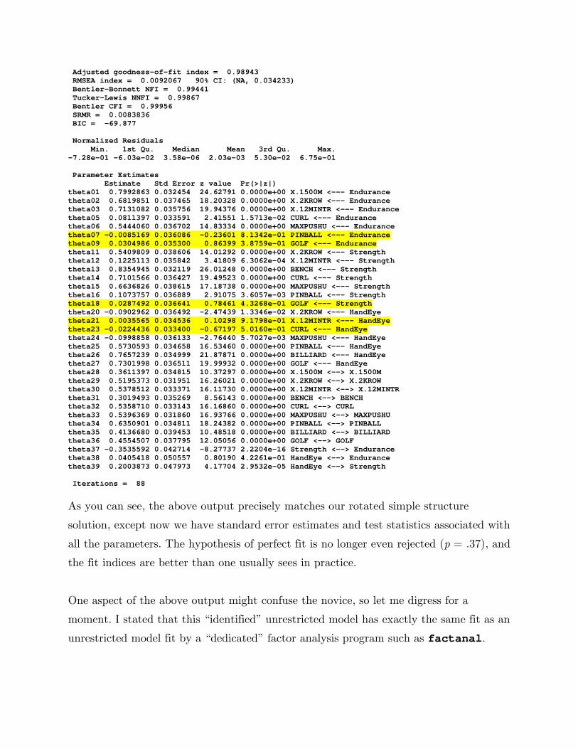
Adjusted goodness-of-fit index = 0.98943 RMSEA index = 0.0092067 90% CI: (NA, 0.034233) Bentler-Bonnett NFI = 0.99441 Tucker-Lewis NNFI = 0.99867 Bentler CFI = 0.99956 SRMR = 0.0083836 BIC = -69.877 Normalized Residuals Min. 1st Qu. Median Mean 3rd Qu. Max. -7.28e-01 -6.03e-02 3.58e-06 2.03e-03 5.30e-02 6.75e-01 Parameter Estimates Estimate Std Error z value Pr(>|z|) theta01 0.7992863 0.032454 24.62791 0.0000e+00 X.1500M <--- Endurance theta02 0.6819851 0.037465 18.20328 0.0000e+00 X.2KROW <--- Endurance theta03 0.7131082 0.035756 19.94376 0.0000e+00 X.12MINTR <--- Endurance theta05 0.0811397 0.033591 2.41551 1.5713e-02 CURL <--- Endurance theta06 0.5444060 0.036702 14.83334 0.0000e+00 MAXPUSHU <--- Endurance theta07 -0.0085169 0.036086 -0.23601 8.1342e-01 PINBALL <--- Endurance theta09 0.0304986 0.035300 0.86399 3.8759e-01 GOLF <--- Endurance theta11 0.5409809 0.038606 14.01292 0.0000e+00 X.2KROW <--- Strength theta12 0.1225113 0.035842 3.41809 6.3062e-04 X.12MINTR <--- Strength theta13 0.8354945 0.032119 26.01248 0.0000e+00 BENCH <--- Strength theta14 0.7101566 0.036427 19.49523 0.0000e+00 CURL <--- Strength theta15 0.6636826 0.038615 17.18738 0.0000e+00 MAXPUSHU <--- Strength theta16 0.1073757 0.036889 2.91075 3.6057e-03 PINBALL <--- Strength theta18 0.0287492 0.036641 0.78461 4.3268e-01 GOLF <--- Strength theta20 -0.0902962 0.036492 -2.47439 1.3346e-02 X.2KROW <--- HandEye theta21 0.0035565 0.034536 0.10298 9.1798e-01 X.12MINTR <--- HandEye theta23 -0.0224436 0.033400 -0.67197 5.0160e-01 CURL <--- HandEye theta24 -0.0998858 0.036133 -2.76440 5.7027e-03 MAXPUSHU <--- HandEye theta25 0.5730593 0.034658 16.53460 0.0000e+00 PINBALL <--- HandEye theta26 0.7657239 0.034999 21.87871 0.0000e+00 BILLIARD <--- HandEye theta27 0.7301998 0.036511 19.99932 0.0000e+00 GOLF <--- HandEye theta28 0.3611397 0.034815 10.37297 0.0000e+00 X.1500M <--> X.1500M theta29 0.5195373 0.031951 16.26021 0.0000e+00 X.2KROW <--> X.2KROW theta30 0.5378512 0.033371 16.11730 0.0000e+00 X.12MINTR <--> X.12MINTR theta31 0.3019493 0.035269 8.56143 0.0000e+00 BENCH <--> BENCH theta32 0.5358710 0.033143 16.16860 0.0000e+00 CURL <--> CURL theta33 0.5396369 0.031860 16.93766 0.0000e+00 MAXPUSHU <--> MAXPUSHU theta34 0.6350901 0.034811 18.24382 0.0000e+00 PINBALL <--> PINBALL theta35 0.4136680 0.039453 10.48518 0.0000e+00 BILLIARD <--> BILLIARD theta36 0.4554507 0.037795 12.05056 0.0000e+00 GOLF <--> GOLF theta37 -0.3535592 0.042714 -8.27737 2.2204e-16 Strength <--> Endurance theta38 0.0405418 0.050557 0.80190 4.2261e-01 HandEye <--> Endurance theta39 0.2003873 0.047973 4.17704 2.9532e-05 HandEye <--> Strength Iterations = 88
As you can see, the above output precisely matches our rotated simple structure
solution, except now we have standard error estimates and test statistics associated with
all the parameters. The hypothesis of perfect fit is no longer even rejected (p = .37), and
the fit indices are better than one usually sees in practice.
One aspect of the above output might confuse the novice, so let me digress for a
moment. I stated that this “identified” unrestricted model has exactly the same fit as an
unrestricted model fit by a “dedicated” factor analysis program such as factanal.

However, in this case, we see a chi square statistic of 13.016, while in our previous
investigation using factanal gave a chi square of 12.94. Why the discrepancy?
The answer is that the chi square statistic is, in general, computed by multiplying the
maximum likelihood discrepancy function by a “multiplier.” Most general purpose
structural equation modeling programs use a multiplier of 1N - , while many dedicated
factor analysis programs use the “Bartlett multiplier”
4 5
13 6
p mN
+- - -
If you examine the factanal output with the command
> exploratory$criteria objective counts.function counts.gradient 0.01302917 11.00000000 11.00000000
you discover that the discrepancy function is .01302917. The Bartlett multiplier is
992.1667, which when multipled by the discrepancy function gives the stated chi square
value of 12.94. If we multiply the discrepancy by 1N - , we obtain 13.016, the value
given by sem. We can also examine the discrepancy function directly, with the
command
> base.model.fit$criterion [1] 0.01302917
The next step, according to Jöreskog (1978), is to pare down the model by eliminating
factor loadings that are not significant, and then re-estimating the model. If we
eliminate all paths that are not significant with p < .05, two-tailed, this amounts to
eliminating all paths with z-statistics less than 1.96 in absolute value. I highlighted all
the loading (directed) paths in the output above. Effectively eliminating them by
placing ## in front of them, and fitting the revised model, we get
Model Chisquare = 14.824 Df = 17 Pr(>Chisq) = 0.60814 Chisquare (null model) = 2330.1 Df = 36 Goodness-of-fit index = 0.99678 Adjusted goodness-of-fit index = 0.99147 RMSEA index = 0 90% CI: (NA, 0.024988) Bentler-Bonnett NFI = 0.99364 Tucker-Lewis NNFI = 1.002 Bentler CFI = 1

SRMR = 0.010374 BIC = -102.61 Normalized Residuals Min. 1st Qu. Median Mean 3rd Qu. Max. -7.48e-01 -1.48e-01 -9.49e-06 -1.56e-02 6.34e-02 1.12e+00 Parameter Estimates Estimate Std Error z value Pr(>|z|) theta01 0.798679 0.032453 24.6106 0.0000e+00 X.1500M <--- Endurance theta02 0.682514 0.037419 18.2398 0.0000e+00 X.2KROW <--- Endurance theta03 0.714667 0.035439 20.1663 0.0000e+00 X.12MINTR <--- Endurance theta05 0.079109 0.033130 2.3878 1.6949e-02 CURL <--- Endurance theta06 0.545619 0.036620 14.8994 0.0000e+00 MAXPUSHU <--- Endurance theta11 0.540617 0.038419 14.0717 0.0000e+00 X.2KROW <--- Strength theta12 0.123926 0.034505 3.5915 3.2875e-04 X.12MINTR <--- Strength theta13 0.837604 0.032037 26.1446 0.0000e+00 BENCH <--- Strength theta14 0.703326 0.034641 20.3035 0.0000e+00 CURL <--- Strength theta15 0.663589 0.038425 17.2695 0.0000e+00 MAXPUSHU <--- Strength theta16 0.103959 0.031970 3.2517 1.1471e-03 PINBALL <--- Strength theta20 -0.085985 0.033327 -2.5801 9.8785e-03 X.2KROW <--- HandEye theta24 -0.094708 0.033368 -2.8382 4.5363e-03 MAXPUSHU <--- HandEye theta25 0.574036 0.034090 16.8387 0.0000e+00 PINBALL <--- HandEye theta26 0.762281 0.034516 22.0849 0.0000e+00 BILLIARD <--- HandEye theta27 0.740866 0.034353 21.5664 0.0000e+00 GOLF <--- HandEye theta28 0.362112 0.034793 10.4077 0.0000e+00 X.1500M <--> X.1500M theta29 0.520594 0.031931 16.3039 0.0000e+00 X.2KROW <--> X.2KROW theta30 0.536656 0.033361 16.0861 0.0000e+00 X.12MINTR <--> X.12MINTR theta31 0.298420 0.035146 8.4910 0.0000e+00 BENCH <--> BENCH theta32 0.538503 0.032873 16.3815 0.0000e+00 CURL <--> CURL theta33 0.540087 0.031881 16.9410 0.0000e+00 MAXPUSHU <--> MAXPUSHU theta34 0.635539 0.034737 18.2958 0.0000e+00 PINBALL <--> PINBALL theta35 0.418927 0.038344 10.9256 0.0000e+00 BILLIARD <--> BILLIARD theta36 0.451118 0.037473 12.0386 0.0000e+00 GOLF <--> GOLF theta37 -0.354331 0.042603 -8.3170 0.0000e+00 Strength <--> Endurance theta38 0.049396 0.042759 1.1552 2.4800e-01 HandEye <--> Endurance theta39 0.202231 0.041354 4.8902 1.0071e-06 HandEye <--> Strength Iterations = 23
A final step, according to Jöreskog, is to check modification indices to see if any zero
loadings might be relaxed.
> mod.indices(pared.model.fit)
The results show that no potential loading from a factor to an observed variable makes
the list of highest modification indices in the A matrix, and only one of them suggests a
significant improvement in the chi square statistic, because the significance value for a 2c with one degree of freedom is 3.84.
5 largest modification indices, A matrix: GOLF:X.2KROW BILLIARD:X.2KROW X.2KROW:GOLF CURL:GOLF X.1500M:MAXPUSHU 3.933301 2.005178 1.417790 1.128748 0.968813 5 largest modification indices, P matrix: X.2KROW:GOLF X.12MINTR:GOLF X.2KROW:BILLIARD MAXPUSHU:X.1500M MAXPUSHU:X.12MINTR 4.427690 2.845399 2.576033 2.101112 2.016665

This final model has fit statistics that are incredibly good. The point estimate for the
RMSEA is zero, and the p-value for the test of perfect fit is .61. The hypothesis of
perfect fit cannot be rejected.
Before ending this discussion, I’d like to sound some cautionary notes, and add some
food for thought. First and foremost, the statistics generated by sem and several other
programs like it assume that (a) a sample covariance matrix with (b) a Wishart
distribution is being analyzed. The distribution theory, overall test of fit, and standard
error estimates are all based on that assumption. Assumption (a) is clearly violated in
this situation, as, true to tradition, we actually analyzed the correlation matrix. Now, in
a sense, a correlation matrix is a covariance matrix, but the sample correlation matrix
does not have the same distribution as the sample covariance matrix from which it is
calculated. To see why, simply look at each element of the correlation matrix. The
diagonal entries do not vary randomly — they are always 1 — while the elements on
the diagonal of a sample covariance matrix are, of course, free to vary. Lawley and
Maxwell (1970) pointed this out in their book on factor analysis, and showed the extent
of the error in the standard error estimates that could result from analyzing the sample
correlation matrix as though it were a correlation matrix. The earliest commercial
software program, LISREL, was based on a computational engine that assumed a
covariance matrix was being analyzed. For years, LISREL produced incorrect standard
error estimates from a sample correlation matrix, and, in fact, featured examples of the
same in its manual. The chi square statistic and parameter estimates are not affected by
this error when a factor model is estimated, but the standard errors can be substantially
in error.
In practice, assumption (b), which amounts in practice to an assumption of multivariate
normality, is also violated frequently. Although “asymptotically distribution free”
(ADF) methods are available to compensate for this, they don’t work very well unless
sample sizes are quite large.
If you think carefully about what we did in our two approaches to confirmatory factor
analysis, you will realize that a number of aspects were questionable, because the

procedures violated some long established principles of statistical analysis. In addition to
some truly questionable aspects of the procedures, other things we did were somewhat
arbitrary. For example, we decided to stop freeing up factor loadings in our first
approach, when the modification indices showed we could continue to produce
significant improvements in the overall fit statistic. In the second procedure, we used
the .05 significance level to establish our cutoff for deciding if a loading is
“insignificant.” What would have happened if we’d considered familywise error rate?
These are issues we will discuss in class.
Related Documents