Concurrent Hydroclimatic Hazards from Catchment to Global ...

Concurrent Hydroclimatic Hazards from

Catchment to Global Scales

by

Paolo De Luca

Doctoral Thesis

Submitted in partial fulfilment of the requirements for the award of

Doctor of Philosophy (PhD) of Loughborough University

(August 2019)

© by Paolo De Luca (2019)

Thesis Commons version

ii

iii

Abstract

Interactions between multiple hazards can cause socio-economic damages that exceed those expected

by the individual hazard components. Over the past decade, the multi-hazards paradigm has emerged

to the extent that the Sendai Framework for Disaster Risk Reduction 2015-2030 advocated a multi-

hazard approach. This thesis examines three types of concurrent hydroclimatic hazards that can occur

at catchment to global scales.

The first multi-hazard is the link between multi-basin flooding (MBF) and extra-tropical cyclones

(ETCs) over Great Britain during the period 1975-2014. Results show that during the most

geographically widespread MBF episode, up to 108 river catchments (or ~46% of the study area)

recorded a peak flow annual maximum within a 16-day window. Most extreme MBF episodes were

linked to cyclonic Lamb Weather Types (LWTs), atmospheric rivers and very severe gales. These

episodes were associated with significant socio-economic impacts due to widespread flooding.

The second hazard was observed (1971-2000) and projected (2011-2100) LWTs, whose seasonal

frequency and persistence are associated with multi-hazards over the British Isles (BI). Daily sea-level-

pressure data from two reanalyses products, one subjective weather pattern catalogue and an ensemble

of 10 Atmosphere-Ocean General Circulation Models (AOGCMs) were used to compute LWTs.

Results showed that the AOGCMs are overall able to reproduce historical weather pattern persistence,

which, along with annual frequency (p-value <0.01), is projected to significantly increase anticyclonic

and decrease cyclonic LWTs, in summer and autumn respectively. This implies a higher risk of

drought, heatwaves and air pollution events in summer but reduced likelihood of flooding and severe

gales in autumn by the end of the 21st century. By 2100, the AOGCMs suggest a significant increased

risk of concurrent flood-wind hazards during winter. In summer, the strength of the nocturnal Urban

Heat Island (UHI) of London is expected to intensify by about 0.15 °C by the end of the century,

contributing to higher chances of combined heatwave-air pollution events.

The third type of multi-hazard investigated was the spatio-temporal concurrence of global wet and dry

hydrological extremes, during the 1950-2014 period. The analysis was conducted using the monthly

self-calibrated Palmer Drought Severity Index based on the Penman-Monteith model (sc_PDSI_pm)

– a global gridded dataset that has been applied in similar, but single-hazard, investigations. Results

showed that the land area impacted by extreme dry and wet-dry events significantly increased over the

iv

observational period. The most geographically widespread wet-dry event covered a total area of 21

million km2 (or 14% of the global land area) with documented flood and drought impacts over diverse

regions. Two new metrics were developed to provide more insight into the combined wet and dry

hazards: the wet-dry (WD) ratio and the extreme transition (ET) time interval. The former quantifies

the predominance of wet or dry extremes over a given area, whereas the ET measures the average

separation time between the opposite extremes (i.e. between wet to dry or dry to wet transitions). The

WD-ratio reveals a predominance of wet over dry extremes in the USA, northern and southern south

America, northern Europe, north Africa, western China and most of Australia. The ET median for wet

to dry is ~27 months, and 21 months for dry to wet. Global correlations between wet-dry hydrological

extremes and El Niño Southern Oscillation (ENSO), Pacific Decadal Oscillation (PDO) and American

Multidecadal Oscillation (AMO) were also investigated. ENSO and PDO showed similar correlation

patterns, with the former significantly impacting a larger area. On the other hand, the AMO showed

an almost inverse spatial correlation pattern, with an overall larger area impacted.

The findings presented in this thesis could be informative for emergency responders and relief

agencies, disaster risk reduction practitioners, and (re)insurance companies. For instance, multi-basin

flooding co-occurring with ETCs could overwhelm emergency response that depends on support from

neighbouring regions that are similarly affected. Economic damages could exceed those insured by

households and businesses. Projected rises in nocturnal UHI intensity in London could exacerbate

heat-stress and, when combined with episodes of poor air quality, increase the likelihood of health

problems amongst vulnerable groups. Furthermore, concurrent wet and dry hydrological extremes

could be significant for organizations with global assets or sensitive supply chains, and the

hydropower, agricultural and transport sectors more generally. Global maps generated of major wet-

dry events and the WD-ratio could also be integrated into a seasonal forecasting product, to help

stakeholders in hedging the risk. Key opportunities for further research on multi-hazards are future

hydroclimatic projections in the light of anthropogenic climate change and the application of new

statistical techniques that could help in discerning the driving physical processes.

v

Table of Contents

Abstract……………………………………………………………………………………...iii

Glossary……………………………………………………………………………..……….ix

List of Figures………………………………………………………………...……………..xii

List of Tables………………………………………………………………………..…….xviii

Chapter 1: Introduction…………………………………………………………...…..……21

Chapter 2: Literature review…………………………………….………………………...29

2.1 Introduction………………………………………………………………………………………29

2.2 Multi-hazards………………………………………………….………………………………….33

2.2.1 Multi-hazard and risk assessments………………………………………………….…...….37

2.2.2 Storm-driven floods………………………………………………………………………...40

2.3 Weather patterns……………………………………………………………….……………..…..44

2.4 Hydrological extremes and modes of climate variability………………………………………....50

2.4.1 Wet and dry hydrological extremes…………………………………………………………50

2.4.2 Fluvial flooding and modes of climate variability…………………………..………………54

2.5 Summary………………………………………………………………….………………………59

Chapter 3: Extreme multi-basin flooding linked with extra-tropical cyclones………..…61

3.1 Introduction………………………………………………………………………………….…...61

3.2 Peak Flow and SPI Data……………………………………………………………………..……63

3.3 Methods……………………………………………………………………………………..…....66

3.3.1 Quantifying multi-basin flooding episodes…………………………………………..……..66

3.3.2 Metrics……………………………………………………………………………..……….67

3.3.2.1 Flood Yield (FY)…………………………………………………………………....67

3.3.2.2 Basin joining time (Jt)………………………………………………..……………..67

3.3.2.3 ‘Time to peak’ modelling…………………………………………………………...68

3.3.2.4 Flood Index (F-Index)……………………………………………………..………..68

3.3.3 Statistical testing……………………………………………………………………………68

vi

3.3.3.1 Multi-basin episodes……………………………………………………………..…68

3.3.3.2 Basin joining times………………………………………………………….……...69

3.3.3.3 F-Index……………………………………………………………………………..69

3.3.3.4 Multi-basin flooding and Atmospheric Rivers………………………………...……69

3.3.3.5 SPI averages………………………………………………………………………...69

3.3.3.6 Peak flows and very severe gales…………………………………………………...70

3.4 Results……………………………………………………………………………….…………...70

3.4.1 Characterizing severe MBF episodes…………………………………………..…………...70

3.4.2 Relationship to inundation episodes………………………………………………………...77

3.4.3 Relationship to atmospheric patterns……………………………………………………….78

3.4.4 Relationship with antecedent soil moisture conditions……………………………….…….80

3.4.5 Relationship to very severe gales……………………………………………………..….....81

3.5 Discussion…………………………………………………………………………………..…….83

3.5.1 A new multi-basin approach………………………………………………………….…….83

3.5.2 Widespread concurrent impacts………………………………………………………….....83

3.5.3 Compound flood and wind impacts…………………….……………………………….......85

3.5.4 Operational implications………………………………………………………..………..…86

3.5.5 Storms since 2014…………………………………………………………………..………86

3.6 Summary……………………………………………………………………………………….....87

Chapter 4: Past and projected weather pattern persistence associated with multi-hazards

in the British Isles……………………………………………………………………..….....89

4.1 Introduction………………………………………………….……………………………….…..89

4.2 Methods and Data…………………………………………………………………………..…….92

4.2.1 Lamb Weather Types (LWTs)……………………………………………………….……..92

4.2.2 Data………………………………………………………………………………………....94

4.2.3 Persistence and trend analyses………………………………………………………….…..96

4.2.4 Indices of winter flood-wind hazards and summer UHI intensity………………………..…97

4.3 Results………………………………………………………………………………………....…98

4.3.1 Persistence of weather patterns (MME)………………………………………………..…...98

4.3.2 Persistence of weather patterns (by model)………………………………..………………102

4.3.3 Frequency of weather patterns (MMEM)…………………………………………..……...104

4.3.4 Application to future multi-hazards……………………………………………...…….….107

vii

4.4 Discussion and Conclusions…………………………………………………………………….111

4.5 Summary……………………………………………………………………………………...…114

Chapter 5: Concurrent wet and dry hydrological extremes at the global scale…...……116

5.1 Introduction…………………………………………………………………...………………...116

5.2 Data and Methods……………………………………………………………………………….119

5.2.1 Data………………………………………………………………………………………..119

5.2.2 Methods for identifying extreme wet, dry, neutral and wet-dry events…………………….119

5.2.3 Wet-dry metrics…………………………………………………………………………...120

5.2.4 Correlation tests……………………………...……………………………………………122

5.3 Results…………………………………………………………...……………………………...122

5.3.1 Land area impacted by extreme wet, dry, neutral and wet-dry events……………………...122

5.3.2 Concurrent global flood and drought events………………………………………………125

5.3.3 Wet-dry (WD) ratio………………………………………………………………………..128

5.3.4 Extreme transitions (ET)…………………………………………………………………..129

5.3.5 Correlations with Climate Indices…………………………...…………………………….132

5.4 Discussion and Conclusions…………………………………………………………………….136

5.5 Summary………………………………………………………………………………………...138

Chapter 6: Discussion……………………………………………………………………..140

6.1 Overarching theme…………………………………………………...……………………….…140

6.2 Research contributions in context…...…………………………………..…….……….………..143

6.3 Summary……………………………………………………………………….………………..145

Chapter 7: Conclusions……………………………………………………………………147

7.1 Concurrent flood-wind hazards………………………………………………………………….147

7.2 Weather pattern persistence and multi-hazards………………………………………………….149

7.3 Concurrent wet and dry hydrological extremes………………………………………………….151

7.4 The climate is already changing, what about us?...........................................................................152

7.5 Concluding remarks about multi-hazards……………...………………………………………..154

Annex 1………………………………………………………………….……...………….156

A.1 Supplementary Information Chapter 3……………………………………...………156

viii

A.1.1 Figures……………………………………………………………………….……………….156

Annex 2…………………………………………………………………..…...……………160

A.2 Supplementary Information Chapter 4……………………………………...……....160

A.2.1 Methods…………………………………………………………………………….………...160

A.2.1.1 CMIP5, reanalyses and Lamb’s catalogue…………………………………………...160

A.2.1.2 Statistical methods and analyses……………………………………………………..161

A.2.1.2.1 2-day persistence…………………………………………………………..161

A.2.1.2.2 Seasonal trends…………………………………………………………...162

Annex 3………………………………………………………………………...…………..163

A.3 The published article within the journal Environmental Research Letters - Chapter 3

of this thesis…………………………………………………….…………………………..163

References………………………………………………………………………………….176

ix

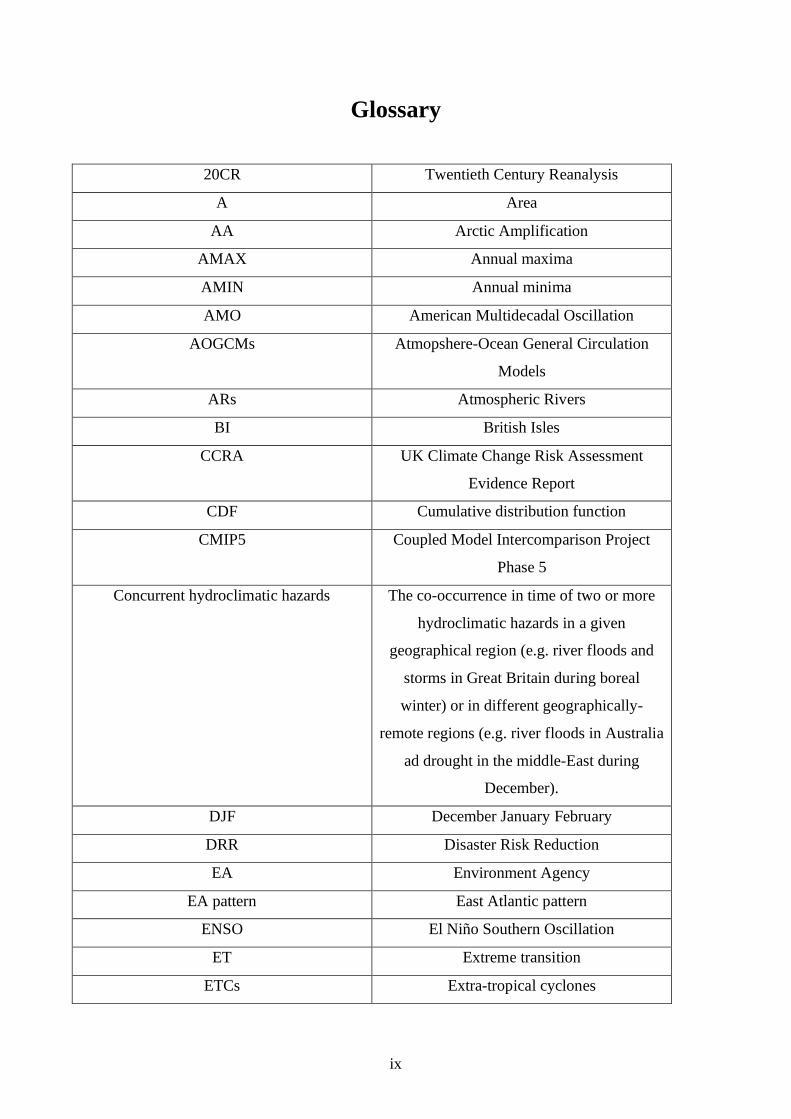
Glossary

20CR Twentieth Century Reanalysis

A Area

AA Arctic Amplification

AMAX Annual maxima

AMIN Annual minima

AMO American Multidecadal Oscillation

AOGCMs Atmopshere-Ocean General Circulation

Models

ARs Atmospheric Rivers

BI British Isles

CCRA UK Climate Change Risk Assessment

Evidence Report

CDF Cumulative distribution function

CMIP5 Coupled Model Intercomparison Project

Phase 5

Concurrent hydroclimatic hazards The co-occurrence in time of two or more

hydroclimatic hazards in a given

geographical region (e.g. river floods and

storms in Great Britain during boreal

winter) or in different geographically-

remote regions (e.g. river floods in Australia

ad drought in the middle-East during

December).

DJF December January February

DRR Disaster Risk Reduction

EA Environment Agency

EA pattern East Atlantic pattern

ENSO El Niño Southern Oscillation

ET Extreme transition

ETCs Extra-tropical cyclones

x

EVT Extreme value theory

F-Index Flood Index

FY Flood yield

GB Great Britain

GCM Global Climate Model

GDP Gross domestic product

HAs Hydrometric Areas

IPCC Intergovernmental Panel on Climate Change

IVT Integrated vapour transport

JJA June July August

Jt Joining time

L Window length

LWTs Lamb Weather Types

MAM March April May

MBF Multi-basin flooding

mFY Multi-basin Flood Yield

MME Multi-model ensemble

MMEM Multi-model ensemble mean

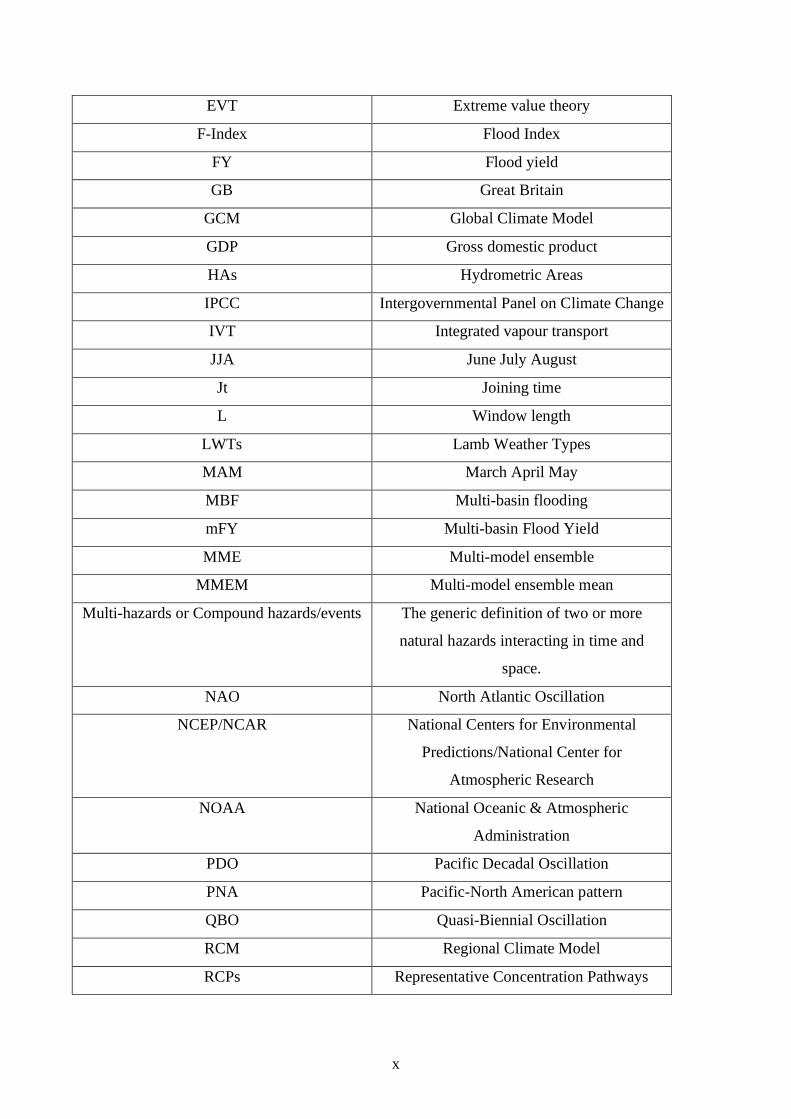
Multi-hazards or Compound hazards/events The generic definition of two or more

natural hazards interacting in time and

space.

NAO North Atlantic Oscillation

NCEP/NCAR National Centers for Environmental

Predictions/National Center for

Atmospheric Research

NOAA National Oceanic & Atmospheric

Administration

PDO Pacific Decadal Oscillation

PNA Pacific-North American pattern

QBO Quasi-Biennial Oscillation

RCM Regional Climate Model

RCPs Representative Concentration Pathways

xi

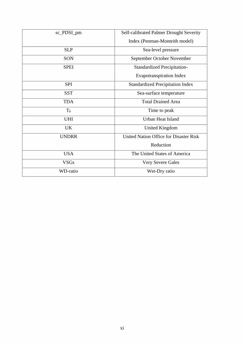
sc_PDSI_pm Self-calibrated Palmer Drought Severity

Index (Penman-Monteith model)

SLP Sea-level pressure

SON September October November

SPEI Standardized Precipitation-

Evapotranspiration Index

SPI Standardized Precipitation Index

SST Sea-surface temperature

TDA Total Drained Area

Tp Time to peak

UHI Urban Heat Island

UK United Kingdom

UNDRR United Nation Office for Disaster Risk

Reduction

USA The United States of America

VSGs Very Severe Gales

WD-ratio Wet-Dry ratio

xii

List of Figures

Figure 1.1 Thesis structure…………………………………………………………………………...28

Figure 2.1 Literature review sections’ links with research chapters………………………………….29

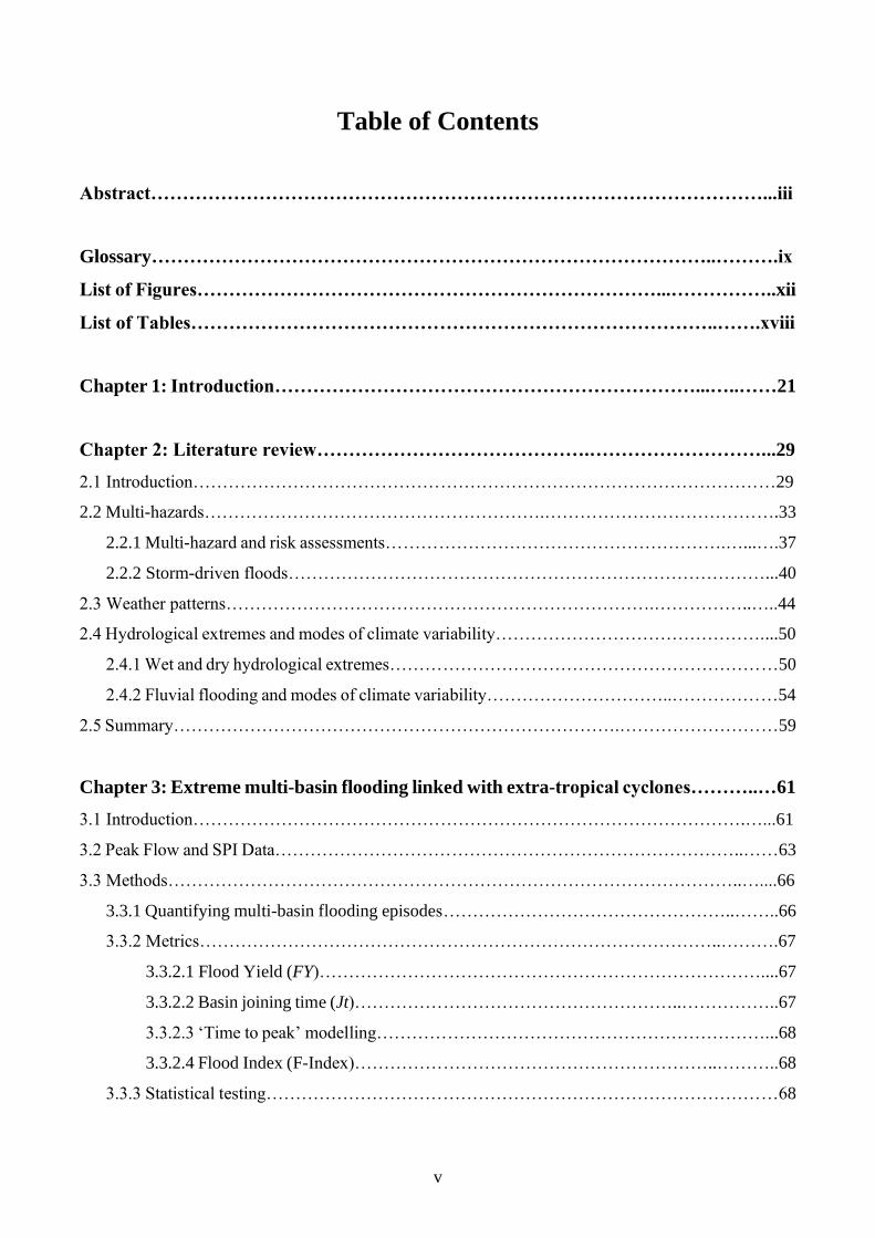
Figure 3.1 Network of hydrological stations and related basin areas used in the analyses. The 261 non-

nested gauges were selected from an initial network of 649 (Annex A.1.1 Figure S3.1) based on record

length, and geographic coverage. Some areas are under-represented (e.g. east England) because they

are either ungauged or do not have data for the 1975-2014 period………………………………...….65

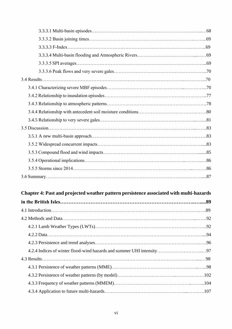
Figure 3.2 Distribution of basins contributing to the extreme MBF episodes in GB during 1975-2014

for six time window lengths (L) (event set E). The maps show respectively: (a) L = 1-day (dmax =

27/12/1979); (b) L = 2-days (dmax = 30/10/2000); (c) L = 4-days (dmax = 01/01/2003); (d) L = 6-days

(dmax = 30/10/2000); (e) L = 8-days (dmax = 02/12/1992); and (f) L = 16-days (dmax = 01/02/1995).

Flood Yield (FY) is a severity metric that represents each basin's peak flow AMAX normalized by the

relative basin area………………………………………………………………………………….....72

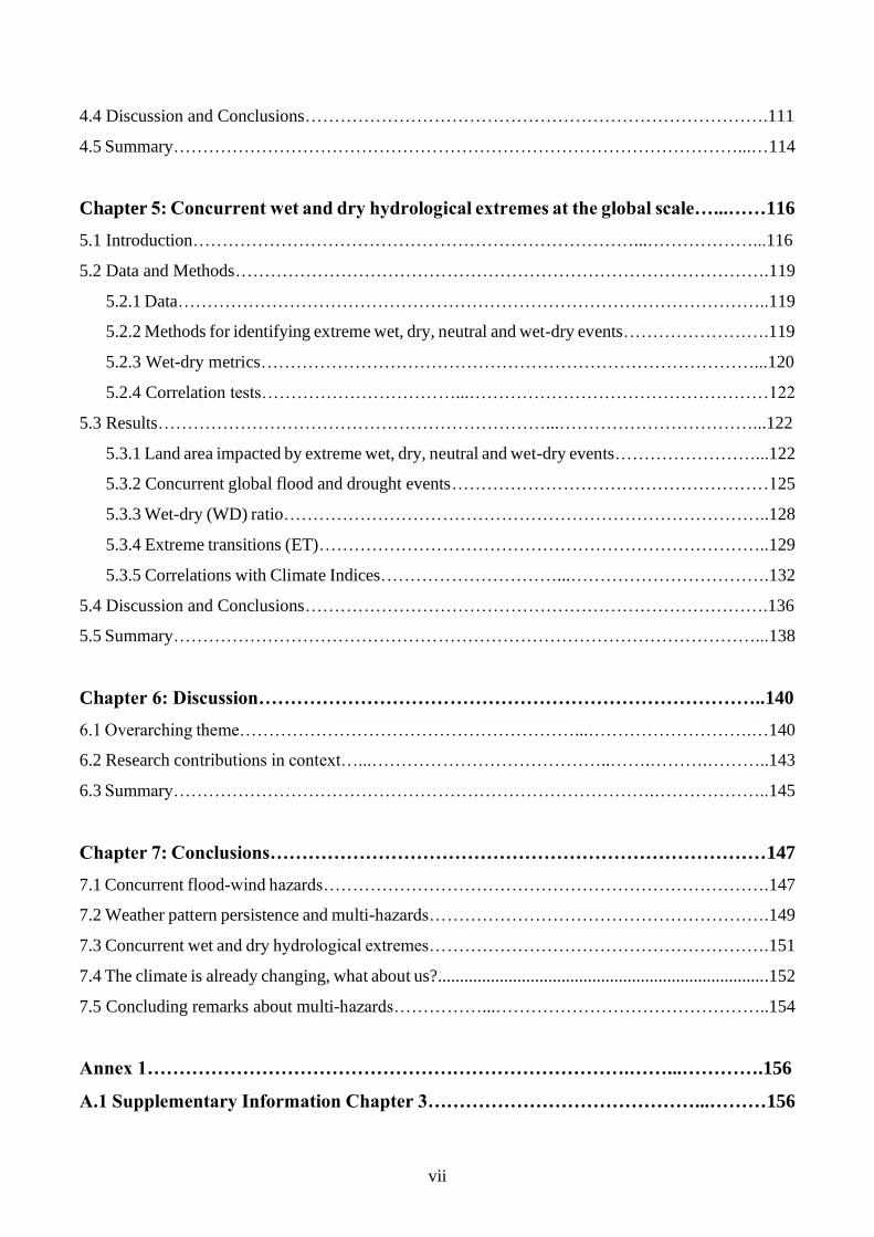
Figure 3.3 Characteristics of the extreme MBF episodes (event set E), compared to event sets A, B, C

and D. (a) Maximum number (i.e. ng) of basins with concurrent AMAX versus window length L,

defining the most extreme episodes (i.e. event set E); (b) as in (a) but for the total study area affected

(i.e. TDA); (c) temporal distribution of peak flow AMAX occurrences for the extreme episodes in

event sets A-E; and (d) frequency of LWTs associated with event sets A-E with respect to their

expected occurrence, calculated as a Flood Index (Wilby and Quinn, 2013). Significance was

determined using the Binomial test. LWTs shown are based on event set E; event sets A-D also contain

other LWTs (Annex A.1.1 Figure S3.2)………………………………………………………………74

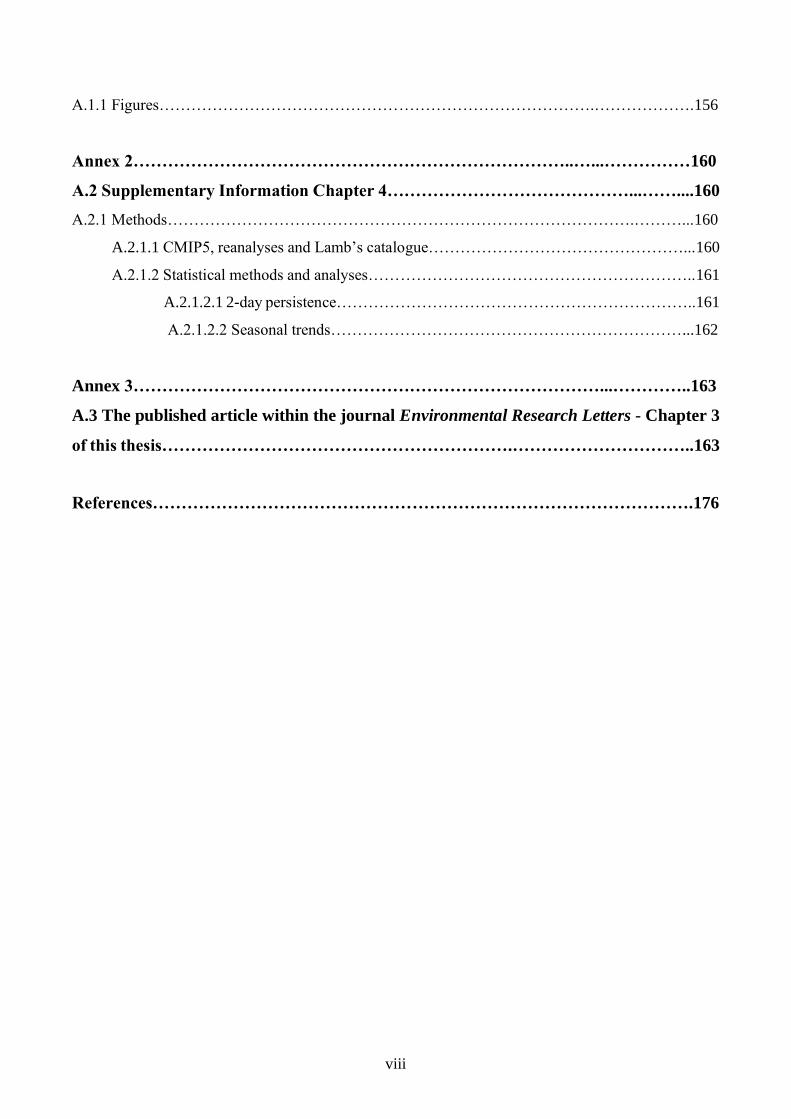
Figure 3.4 Distribution and relative frequency of occurrence of AMAX within event sets B, C, D and

E. (a) Event set B; (b) event set C; (c) event set D; and (d) event set E. The colour scale is a ratio (i.e.

from 0 to 1) of AMAX occurrences in a given basin relative to the basin with the largest number in

that panel, with dark colours indicating most occurrences…………………………………..………..76

xiii

Figure 3.5 Mean Standardized Precipitation Index (SPI) for episodes within event set B for each

window length (L) and SPI time scale (24-1 Months). Green lines are episode SPI averages and the

black line represents the overall (40-year, 1975-2014) SPI average i.e. zero by definition. All episodes

have SPI that are significantly different from the long-term mean at 99% level (t-test, not paired).…..81

Figure 3.6 Number of Very Severe Gales (VSGs) versus extreme multi-basin Flood Yield (mFY)

episodes belonging to event set C for each water year (1975-2014). Black circles = 12-Month SPI < -

0.3; Grey circles = -0.3 < 12-Month SPI < 0.4; White circles = 12-Month SPI > 0.4. n = 20 represents

the 50% most extreme VSG and n = 12 the 30% most extreme mFY episodes…………..…………....82

Figure 4.1 Grid points used to calculate Jenkinson flow and vorticity terms for the British Isles (BI).

Numbers refer to those points used in Equations 4.1 to 4.5…………………………………..…….…94

Figure 4.2 Persistence of the seven main LWTs plus unclassified (U) type under RCP8.5. Persistence

is calculated for (a) summer, (b) autumn, (c) winter and (d) spring, for the historical 1980s period

(1971-2000) and under RCP8.5 by the 2020s (2011-2040), 2050s (2041-2070) and 2080s (2071-2100).

Boxplots show distributions of persistence in each LWT, for the 10-member AOGCM ensemble,

compared with 20CR, NCEP and the Lamb’s catalogue. Segments show the minimum, 1st quartile,

median, 3rd quartile and maximum. Outliers are shown by dots………………………………..……..99

Figure 4.3 Persistence of the seven main LWTs plus unclassified (U) type under RCP4.5. Persistence

is calculated for (a) summer, (b) autumn, (c) winter and (d) spring, for the historical 1980s period

(1971-2000) and under RCP4.5 by the 2020s (2011-2040), 2050s (2041-2070) and 2080s (2071-2100).

Boxplots show distributions of persistence in each LWT, for the 10-member AOGCM ensemble,

compared with 20CR, NCEP and the Lamb’s catalogue. Segments show the minimum, 1st quartile,

median, 3rd quartile and maximum. Outliers are shown by

dots.………………………………………………..………………………………………………..101

Figure 4.4 Persistence of selected LWTs and seasons for individual AOGCMs under RCP8.5. (a) A-

type (summer), (b) C-type (autumn), (c) W-type (winter) and (d) S-type (spring) in the 1980s compared

with the 2020s, 2050s and 2080s under RCP8.5. Persistence is shown for individual AOGCMs

alongside the MMEM, 20CR, NCEP and Lamb’s catalogue. Asterisks (*) show model runs with

persistence outside the 95% confidence intervals of the boot-strapped (n=1,000) estimates for the

1980s, shown here as black T-bars………………………………………………………..…………103

xiv

Figure 4.5 Persistence of selected LWTs and seasons for individual AOGCMs under RCP4.5. (a) A-

type (summer), (b) C-type (autumn), (c) W-type (winter) and (d) S-type (spring) in the 1980s compared

with the 2020s, 2050s and 2080s under RCP4.5. Persistence is shown for individual AOGCMs

alongside the MMEM, 20CR, NCEP and Lamb’s catalogue. Asterisks (*) show model runs with

persistence outside the 95% confidence intervals of the boot-strapped (n=1,000) estimates for the

1980s, shown here as black T-bars………………………………………..………..……………..…104

Figure 4.6 Projected annual frequencies for selected LWTs and seasons under RCP8.5. Frequencies

are shown as MMEM for (a) summer anticyclonic A, (b) autumn cyclonic C, (c) winter westerly W

and (d) spring southerly S LWTs under RCP8.5 (2006-2100). MMEM trends are statistically

significant at the 1% level (p-value <0.01, modified Mann-Kendall test). Shaded areas represent the

95% confidence intervals of the MMEM. The trend lines refer to the Sen’s slopes calculated with the

modified Mann-Kendall test……………………………………………………………...…..……..105

Figure 4.7 Projected annual frequencies for selected LWTs and seasons under RCP4.5. Frequencies

are shown as MMEM for (a) summer anticyclonic A, (b) autumn cyclonic C, (c) winter westerly W

and (d) spring southerly S LWTs under RCP4.5 (2006-2100). MMEM trends are statistically

significant at the 1% and 5% levels (p-value <0.01 and <0.05, modified Mann-Kendall test). Shaded

areas represent the 95% confidence intervals of the MMEM. The trend lines refer to the Sen’s slopes

calculated with the modified Mann-Kendall test…………………………………………………….106

Figure 4.8 F-Score for LWTs associated with concurrent flood-wind hazards during winter DJF. The

F-Score is shown per each CMIP5 AOGCM, MMEM, NCEP, 20CR and Lamb’s subjective catalogue

for the 1980s, 2020s, 2050s and 2080s periods under RCP8.5. The LWTs used for calculating the F-

Score are associated with concurrent multi-basin floods and wind hazards within Great Britain (GB)

(De Luca et al., 2017). The 1980s MME F-Score were estimated from the mean of n=1,000 boot-

strapped samples. The AOGCMs 1980s confidence intervals bars are not shown for simplicity because

they are vanishingly narrow……………………………………………………………………….108

Figure 4.9 F-Score for LWTs associated with concurrent flood-wind hazards during winter DJF. The

F-Score is shown per each CMIP5 AOGCM, MMEM, NCEP, 20CR and Lamb’s subjective catalogue

for the 1980s, 2020s, 2050s and 2080s periods under RCP4.5. The LWTs used for calculating the F-

Score are associated with concurrent multi-basin floods and wind hazards within Great Britain (GB)

xv

(De Luca et al., 2017). The 1980s MME F-Score were estimated from the mean of n=1,000 boot-

strapped samples. The AOGCMs 1980s confidence intervals bars are not shown for simplicity because

they are vanishingly narrow………………………………………………………………………....109

Figure 4.10 UHI in tenths of °C for LWTs associated with concurrent heat-air pollution hazards during

summer JJA. The UHI is shown per each CMIP5 AOGCM, MMEM, NCEP, 20CR and Lamb’s

subjective catalogue for the 1980s, 2020s, 2050s and 2080s periods under RCP8.5. The 1980s MME

UHI were estimated from the mean of n=1,000 boot-strapped samples. The AOGCMs 1980s

confidence intervals bars are not shown for simplicity because they are vanishingly narrow.............110

Figure 4.11 UHI in tenths of °C for LWTs associated with concurrent heat-air pollution hazards during

summer JJA. The UHI is shown per each CMIP5 AOGCM, MMEM, NCEP, 20CR and Lamb’s

subjective catalogue for the 1980s, 2020s, 2050s and 2080s periods under RCP4.5. The 1980s MME

UHI were estimated from the mean of n=1,000 boot-strapped samples. The AOGCMs 1980s

confidence intervals bars are not shown for simplicity because they are vanishingly

narrow.………………………………………………………………………………………………111

Figure 5.1 Percentage (%) of total land area with (a) wet (blue), (b) dry (red) extremes, (c) neutral

(black) and (d) extreme wet + extreme dry (orange) events over the 1950-2014 period. Wet extremes

are sc_PDSI_pm ≥ 3) and dry extremes sc_PDSI_pm ≤ -3 monthly observations. Sen’s slopes and the

significance of the Mann Kendall test (p-values) are shown in each panel.…………..……………...124

Figure 5.2 (a) Most widespread extreme global wet hydrological event (blue colour) and coincident

extreme dry areas (red colour), December 2010. The event was also the most widespread concurrent

wet-dry episode. The percentage (%) of total land area is shown for both wet and dry extremes, along

with the values of the three climate indices (i.e. Niño3.4, PDO and AMO) in December 2010. (b) As

(a) but for the most widespread extreme global dry hydrological event, January 2003. (a)-(b) The

analysis is based on the self-calibrated monthly mean Palmer Drought Severity Index (sc_PDSI_pm)

for the period 1950-2014……………………………………………………………...…………….127

Figure 5.3 Wet-dry (WD) ratio derived for every grid-cell. Blue colours (WD-ratio > 0) mean that the

area experienced more wet than dry hydrological extremes. Red colours (WD-ratio < 0) indicate the

opposite………………………………………………………………………………...………...…128

xvi

Figure 5.4 Extreme transition (ET) time intervals between extreme wet to dry (blue) and between

extreme dry to wet (red). (a) ET as a function of the total percentage (%) of total land area impacted

and (b) cumulative distribution functions (CDFs). The horizontal black line in (b) indicates the 50th

quantile (i.e. median) of the distribution and the blue and red lines the respective ET time intervals.

The two distributions show a statistically significant difference in their means (p-value <<0.01, Mann-

Whitney-Wilcoxon test)…………………………………………………………………………….130

Figure 5.5 Extreme transition (ET) time intervals between extreme wet to wet (blue) and between

extreme dry to dry (red). (a) ET as a function of the total percentage (%) of total land area impacted

and (b) cumulative distribution functions (CDFs). The horizontal black line in (b) indicates the 50th

quantile (i.e. median) of the distribution and the blue and red lines the respective ET time intervals.

The two distributions show a statistically significant difference in their means (p-value <<0.01, Mann-

Whitney-Wilcoxon test). To note that for simplicity only ET with a time interval ≤ 200 months are

shown.…………………………………………………………………………..……………..……131

Figure 5.6 Correlations between extreme wet (sc_PDSI_pm ≥ 3) and dry (sc_PDSI_pm ≤ -3)

hydrological events and (a) Niño3.4, (b) PDO and (c) AMO. For (b) and (c) partial correlations are

performed to remove the Niño3.4 signal. Correlations and partial correlations make use of the

Spearman’s correlation coefficient. Correlations significant at the 5% level (p-value <0.05) are shown

by stippling. The Bonferroni correction was applied to all p-values. In (b) and (c) the ENSO signal has

been removed via partial correlations……………………………………………………………….134

Figure 5.7 Correlations between extreme wet (sc_PDSI_pm ≥ 3) and dry (sc_PDSI_pm ≤ -3)

hydrological events and (a) NAO, (b) PNA and (c) QBO. Correlations and partial correlations make

use of the Spearman’s correlation coefficient. Correlations significant at the 5% level (p-value <0.05)

are shown by stippling. The Bonferroni correction was applied to all p-values…………………......135

Figure 6.1 Annual number of Google Scholar outputs based on the keyword ‘Multi-Hazard’…...…140

Figure S3.1 Initial hydrological network of 649 gauges. The yellow stations are the 261 non-nested

basins used in the analyses, whereas blue stations represent the remaining 388 nested stations excluded

from the study because they are located upstream from a non-nested gauge……………………...…156

xvii

Figure S3.2 Lamb Weather Types’ (LWTs) observed percentages of occurrence for all event sets (A-

E). (a) Event set A; (b) event set B; (c) event set C; (d) event set D; and (e) event set E. All with

replicated dates excluded……………………………………………………………………………157

Figure S3.3 Lamb Weather Types’ F-Index (Wilby and Quinn, 2013) calculated for event sets B, C,

D and E with respect to single-basin occurrences (i.e. event set A). Significance was determined using

Binomial test, but with event set A used as expected values. LWTs shown are based on event set E;

event sets B-D also contain other LWTs…………………………………………………………….158

Figure S3.4 Extreme multi-basin flooding episodes’ joining times (event set E). (a) L = 1-day (dmax =

27/12/1979); (b) L = 2-days (dmax = 30/10/2000); (c) L = 4-days (dmax = 01/01/2003); (d) L = 6-days

(dmax = 30/10/2000); (e) L = 8-days (dmax = 02/12/1992); and (f) L = 16-days (dmax = 01/02/1995).

Days are ordered chronologically (e.g. Day = 16 represents dmax for L = 16-days)………………..159

xviii

List of Tables

Table 2.1 Main terminology used in the thesis……………………………………………………30-31

Table 2.2 Classification of natural hazards………………………………………………………..….33

Table 2.3 Relationships between natural hazards………………………………………………….....34

Table 2.4 Types of interactions and coincidence between natural hazards…………………………...35

Table 2.5 Anthropogenic processes affecting the triggering of one or more natural hazards…...…..36

Table 2.6 Interactions between human activities and natural hazards……………………………....37

Table 3.1 Extreme MBF episodes in GB during 1975-2014 (event set E). Observations are derived

from 19 time windows up to 18 days prior dmax; see main text for details. (a) Window length (L) in

days; (b) Total drained area (TDA, km2) involved in each episode (i.e. sum of the area of all involved

basins); (c) Percentage of TDA of the 261 basins affected by each episode; (d) Percentage of GB land

area affected by each episode; (e) Dates of episodes, where the top row represents dmax; (f) Number of

basins with peak flow AMAX registered on the same day; (g) Total number of basins with peak flow

AMAX per episode; (h) Percentage of total number of basins (out of 261) with concurrent AMAX per

episode; (i) Daily LWT; (j) Average joining time, within an episode, for larger basins (A 1,000km2);

(k) Average joining time for small basins (A <1,000km2). In (j) and (k) uncertainties are 1 standard

error of the mean…………………………………………………………………………….…….79-80

Table 4.1 CMIP5 multi-model sub-ensemble (MME) used in the analyses. The columns show the: (1)

CMIP5 model name; (2) research institute where the model was developed; (3) resolution as latitude

by longitude in degrees; and (4) ensemble member analysed. For all models the historical and RCP8.5

(and RCP4.5) sea-level pressure (SLP) outputs are used to calculate daily LWTs for the BI………....95

Table 4.2 MME statistical significance of LWTs persistence for RCP8.5. Time periods considered are

the 1980s compared to the 2020s, 2050s and 2080s under RCP8.5 during all seasons: summer JJA,

autumn SON, winter DJF and spring MAM. Values shown are the W-statistic from the Mann-Whitney-

xix

Wilcoxon two-tailed test. Statistically significant values (p-value <0.1) are shown in

bold…………………………………………………………………………………………...…..…100

Table 4.3 MME statistical significance of LWTs persistence for RCP4.5. Time periods considered are

the 1980s compared to the 2020s, 2050s and 2080s under RCP4.5 during all seasons: summer JJA,

autumn SON, winter DJF and spring MAM. Values shown are the W-statistic from the Mann-Whitney-

Wilcoxon two-tailed test. Statistically significant values (p-value <0.1) are shown in

bold………………………………………………………………………………………………….102

Table 4.4 Sen’s slopes of MMEM seasonal LWTs frequencies for RCP8.5 and RCP4.5. The slopes

are calculated using a modified Mann-Kendall trend test over the 2006-2100 period. Four LWTs are

shown: anticyclonic (A) for summer JJA; cyclonic (C) autumn SON; westerly (W) winter DJF and

southerly (S) spring MAM. MMEM statistical significance is shown as * p-value <0.05 and ** p-value

<0.01……………………………………………………………………...…………...…..………...107

Table 6.1 Suggested open research questions within the field of multi-hazards…………………….142

xx

21

Chapter 1

Introduction

Weather, climate and hydrological extremes around the world pose significant socio-economic threats

and a general consensus is that they will become even more extreme due to anthropogenic climate

change (IPCC, 2018).

Within a warmer world, an increase in extreme precipitation events is expected (Chan et al., 2014;

Fischer and Knutti, 2016; IPCC, 2018, 2012; Lenderink and Fowler, 2017; Liu and Allan, 2013; Min

et al., 2011) because of a larger availability of water vapour that generates from an increased water

holding capacity of the atmosphere (Trenberth, 2011). Such increases in precipitation extremes may

also eventually lead to more frequent and/or severe flooding events (Arnell and Gosling, 2016; IPCC,

2012), also accompanied by a shift in the timing of floods (Blöschl et al., 2017) and projected rising

global flood risk in the future (Winsemius et al., 2016). Moreover, a shift in the global mean

temperature, is expected to translate into more extreme heatwaves with related human heat-stress

projected to impact our everyday lives and businesses (IPCC, 2018; Matthews et al., 2017; Rahmstorf

and Coumou, 2011). There is also medium confidence that some regions in the world are expected to

experience more severe and longer droughts (Dai, 2012; IPCC, 2018; Liu and Allan, 2013;

Prudhomme et al., 2014; Trenberth et al., 2013) and even tropical cyclones may become more intense,

with their frequency unchanged or even decreased (Emanuel, 2005, 2013; IPCC, 2012; Knutson et al.,

2010; Oouchi et al., 2006; Sobel et al., 2016; Webster et al., 2005).

Changes in extreme events also increase their associated economic damages, with an average annual

losses from 1980 ranging from a few US$ billion to about 354 US$ billion, the latter reached in 2011,

the costliest year ever recorded (IPCC, 2012; Kates et al., 2006; Munich Re, 2017a). Studies also show

that most of the increase in damages were due to societal changes and not to changes in extreme events,

(e.g. Changnon et al., 2000; Pielke et al., 2008; Weinkle et al., 2012). Flooding events around the

world had significant impacts, with 5,725 events causing 220,477 fatalities and economic losses of

1,007 US$ billion over the period 1980-2017 and with the vast majority of these occurring in Asia

(Munich Re, 2017a). On the other hand, heatwaves and wildfires, within the same time-period, caused

less economic damages (129 US$ billion) and were also fewer in number with 992 events recorded by

Munich Re. However, the number of heat-related fatalities (~165,000) were almost as high as those

for flooding (Munich Re, 2017a), although these numbers may slightly change depending on the

22

database selected. The number of winter storms, for example extra-tropical cyclone (ETC), events

across the globe amounts to 1,232 with impacts mainly affecting western and central Europe, eastern,

central and western United States (USA) and south-east Asia, for a total of 332 US$ billion losses and

28,162 fatalities over the 1980-2017 period (Munich Re, 2017a).

On the other hand, other studies argue that no trends in losses are found when data are normalised by

societal changes (Changnon et al., 2000; Crompton et al., 2011; Crompton and McAneney, 2008;

Pielke et al., 2008; Weinkle et al., 2012). For instance, Crompton et al. (2011) investigated how much

time is needed for US tropical cyclone losses to be attributed to anthropogenic climate change and

found that depending on the Global Climate Model (GCM) used the emergence of such a signal spans

between 120 to 550 years. In a second study, Crompton and McAneney (2008) normalised Australian

insured losses from meteorological hazards and found no trends that could be attributed to

anthropogenic climate change. Weinkle et al. (2012) constructed a global database of tropical cyclone

landfalls and found no increasing trends in the frequency and intensity of tropical cyclones. They

concluded that the observed increasing losses associated with tropical cyclones are to be attributed by

increasing wealth in areas affected by cyclones’ landfall. Hence, investigating such hazards and their

associated socio-economic impacts, and possible links to anthropogenic climate change, is a significant

topic for enquiry.

A significant body of research is being devoted to weather, climate and hydrological extremes and

risks. This literature spans physical processes, from possible dynamical mechanisms linked to Arctic

Amplification (Screen and Simmonds, 2010) that can exacerbate mid-latitude weather and climate

extremes (e.g. Coumou et al., 2018) to disentangling the contribution of thermodynamics and

dynamics to precipitation extremes (Pfahl et al., 2017). Then there is work on the socio-economic

dimensions, for example, how El Niño influences global flood risk (Ward et al., 2014b) and observed

trends in regional flood risk (Slater and Villarini, 2016). Adaptation measures to extreme events are

widely considered too, from strategies to better manage flood risk under climate change (Wilby and

Keenan, 2012) to a newly proposed research framework for natural hazards and associated

vulnerabilities (Di Baldassarre et al., 2018). Last but not least, possible future changes of weather and

climate extremes currently play a major role in advising decision makers and stakeholders, with global

climate projections of temperature and precipitation extremes (Fischer et al., 2013; Fischer and Knutti,

2015; Fischer and Schär, 2010). All these studies once again confirm the urgency to address and solve

climate-related issues, for the benefit of societies and economies around the world.

23

Hydroclimatology is the study of how the climate system is having an influence on the hydrological

cycle as well as how weather, climate and hydrological extremes (such as floods, storms, droughts and

heatwaves) are impacting or might impact society. Moreover, since weather, climate and hydrological

extremes can be considered a significant part of hydroclimatology (and natural hazards), it is also

possible to investigate how these phenomena interact with each other and of course, how they interact

with the climate system itself. Broadly speaking, in the past two decades or so research looking at

interacting natural hazards has grown considerably, such that the new sub-field of multi-hazards (or

compound hazards) has emerged (Asprone et al., 2010; Bovolo et al., 2009; Gill and Malamud, 2014;

Grünthal et al., 2006; Hillier et al., 2015; Kappes et al., 2012a; Perry and Lindell, 2008; Terzi et al.,

2019; Zscheischler et al., 2018). An example of a multi-hazard event could be for instance the

generation of lahars (the mobilisation of ash and tephra deposits due to rainfall) on an active volcano

flanks in Guatemala, that eventually trigger flooding as these deposits add sediments into the

hydrological system (Harris et al., 2006).

The United Nations (UN) Sendai Framework for Disaster Risk Reduction (UNDRR, 2015) highlights

the importance of multi-hazard approaches to disaster risk reduction (DRR) (e.g. early warning

systems) at global, regional, national and local levels. Multi-hazard is defined by UNDRR as i) the

variety of multiple major hazards that a country faces and ii) the context by which these perils may

occur simultaneously, one after the other (i.e. sequentially), or cumulatively over time, by considering

also their potential interrelated effects (UNDRR, 2016). Thus, the investigation of concurrent

hydroclimatic hazards could bring significant benefits to societies and economies, including improved

adaptation strategies for vulnerable societies and increased economic resilience to disasters. For

instance, national risk assessments could be extended to multi-risk assessments, considering multiple

natural hazards and their associated vulnerability and exposure components not as independent

features but as processes that can interact over time, such as interacting fluvial floods and cyclone

storm surges in mega-delta regions (Ikeuchi et al., 2017; Ward et al., 2018), ETCs bringing combined

severe winds and multi-basin flooding episodes (De Luca et al., 2017) and earthquakes eventually

triggering landslides, tsunamis and floods (Kargel et al., 2016; Suleimani et al., 2009).

Multi-hazards research can also bring benefit to global insurance and re-insurance industries, as the

premium paid by households and businesses may only cover single-hazard events, without offering

the possibility to be insured for two or more hazards concurrently impacting an area in a given short

time-window (e.g. flooding with severe winds, De Luca et al., 2017), or longer periods (e.g. wet-dry

fluctuations leading to shrink-swell subsidence events, Collet et al., 2018; Harrison et al., 2012;

24

Pritchard et al., 2015). This is significant because the insurance provider may not have set aside

sufficient funds to cover for losses generated by interacting hazards as, for example, flood and wind

damages may fall under the same insurance claim (Hillier et al., 2015).

The over-arching question of this thesis is: How one can measure concurrent hydroclimatic hazards

at different time and spatial scales? The answer is given through three studies that investigate weather,

climate and hydrological extremes using a diverse set of methodologies and data. The time scales used

in the studies belong to both past and future. For the former, observational data, from the 1950s to

2014 are used, whereas for the latter future climate projections up to 2100 are gathered and analysed.

The spatial scales, on the other hand, are nested and span from the river catchment unit, to the British

Isles (BI) and then eventually to the global scale such that a local, national and global perspective is

provided.

The research questions of the study can be summarised as follows:

For concurrent flood and wind hazards between river basins in Great Britain.

R1: What is the spatio-temporal distribution of multi-basin flooding episodes?

R2: What are the most frequent weather patterns observed during these widespread floods?

R3: How are multi-basin floods, atmospheric rivers (ARs) and very severe gales (VSGs) linked?

For concurrent hazards linked to persistent weather patterns over the British Isles.

R4: How has persistence in weather pattens changed historically?

R5: To what extent can Atmosphere-Ocean General Circulation Models (AOGCMs) reproduce

observed weather pattern persistence over the BI?

R6: How are weather pattern persistence and frequency expected to change in the future under different

Representative Concentration Pathways (RCPs)?

R7: How changes in future weather type persistence might translate into changed risk of winter flood-

wind and summer heatwave-air pollution concurrent hazards?

For concurrent extreme wet and dry hydrological extremes globally.

R8: How observed globally independent and concurrent wet-dry hydrological extreme events changed

in the past?

R9: What were the most spatially extensive independent and concurrent wet-dry hydrological extreme

events?

25

R10: How new metrics can help in better investigate concurrent wet-dry extremes?

R11: How are these extremes related to different modes of climate variability?

Chapter 2 provides a literature review of the three main streams of research to provide the context for

later chapters. The first topic addressed is multi-hazards, with an introduction to the subject along with

material focussing on floods driven by storms. The multi-hazards literature review is strictly connected

to Chapters 3-5, which are introduced below. Then the second topic refers to weather patterns,

specifically the Lamb Weather Types (LWTs) (Jones et al., 1993; Lamb, 1972). This links with the

previous chapters through a discussion on how possible future changes in LWTs may translate into

independent and compound weather and climate extremes. Here the LWTs classification scheme is

broadly described with particular focus on the BI, and their links to atmospheric variables (e.g.

precipitation, temperature and pollutants). The literature review on LWTs therefore introduces Chapter

4 through a generic overview on the use and impacts of LWTs research. Lastly, the third research

stream provides the basis for Chapter 5 which discusses wet-dry hydrological extremes and modes of

climate variability. Here, studies investigating wet and dry hydrological extremes and the links

between three climate indices and extreme river flows at regional and global scales are reviewed.

The first research area (Chapter 3) addresses the over-arching question of concurrent hydroclimatic

hazards by examining multi-hazard (or compound) events (Zscheischler et al., 2018) over GB. Here

the investigation examines extreme multi-basin flooding driven by ETCs (De Luca et al., 2017).

Chapter 3 offers potential insights for stakeholders, emergency planners and policy makers, with also

methods and metrics easily applicable elsewhere in the world. The aim in Chapter 3 is to extend the

typical view of fluvial flooding confined to a single river basin, to coherent flooding across multiple

river basins within a time-frame of up to two weeks (De Luca et al., 2017; Uhlemann et al., 2010). The

chapter then investigates whether such multi-basin flooding events are driven by ETCs impacting the

BI. Evidence that extreme multi-basin flooding is linked to ETCs is relevant to stakeholders, insurance

industry and emergency managers, as during such events combined flood-wind impacts on large scales

may be expected to cause significant socio-economic damages in the absence of adaptation measures.

Chapter 4 addresses the topic of concurrent hydroclimatic hazards by examining future climate

projections of weather patterns (LWTs or atmospheric circulation) (Jenkinson and Collison, 1977;

Jones et al., 1993; Lamb, 1972) and associated metrics that quantify both independent and multi-

hazards. Here, the connection with the main over-arching research question is addressed from both a

qualitative and quantitative perspective by considering how specific synoptic weather patterns can

26

translate into local weather, climate and hydrological extremes (e.g. Burt and Howden, 2013; De Luca

et al., 2017; Pattison and Lane, 2012). The chapter also investigates how specific LWTs can contribute

to concurrent flood-wind hazards and how changes in LWT persistence could affect the nocturnal

Urban Heat Island (UHI) of London and hence combined heatwave-poor air quality events. The results

of the study provide a methodology based on weather pattern persistence, frequency and multi-hazard

metrics that can help improve the understanding of weather and climate risks to a range of vulnerable

communities.

Finally, Chapter 5 investigates concurrent hydroclimatic hazards in terms of interacting wet and dry

hydrological extremes at the global scale, driven by dominant modes of climate variability. The dataset

used to investigate such events is the Palmer Drought Severity Index (PDSI) (Dai et al., 2004) and the

climate indices deployed are the Niño3.4 (Rayner et al., 2003; Trenberth, 1997), Pacific Decadal

Oscillation (PDO) (Mantua and Hare, 2002) and Atlantic Multidecadal Oscillation (AMO)

(Schlesinger and Ramankutty, 1994). Within the study, new metrics for quantifying concurrent wet-

dry hydrological extremes are also introduced. The results obtained bring new insights about multi-

hazards at the global scale, with also scope for incorporating modes of climate variability into

hydrological forecast models. Such findings could benefit stakeholders and companies that rely on

global diversified portfolios and provide information for emergency managers about the timing and

associated spatial distribution of both independent and concurrent wet and dry extreme events.

These three pillars of the research, although different in nature and methodology, share a common

feature which is the quantification of concurrent hydroclimatic hazards at different time and spatial

scales. All the three studies investigate multi-hazards, however the second study addresses the main

topic from a both a qualitative and quantitative point of view. The commonalities running through the

studies are the investigations of natural hazards, that can affect negatively societies and economies

independently of the spatial scales considered and the quantification of their interactions through

various metrics. Moreover, there is hope that the three studies provide useful and new metrics,

information and insights that are valuable for stakeholders, policy makers and insurance companies.

The purpose of the differences between the studies is to show that the over-arching topic of concurrent

hydroclimatic hazards needs to be addressed from a range of perspectives that draws on a

multidisciplinary pool of research techniques and information sources.

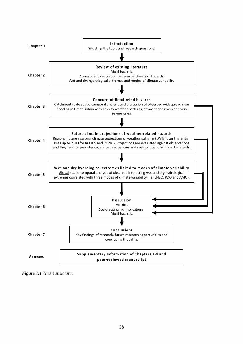
Figure 1.1 provides an overview of the thesis structure and links between the research elements which

variously address concurrent hydroclimatic hazards. The work here presented is organised as follows:

27

a literature review on multi-hazards, weather patterns, wet and dry hydrological extremes and modes

of climate variability is presented in Chapter 2; the extreme multi-basin flooding linked to ETCs

research in GB follows in Chapter 3; future projections and analysis of persistent weather patterns over

the BI as a means of examining future multi-hazards in Chapter 4; globally independent and concurrent

wet and dry hydrological extremes driven by modes of climate variability in Chapter 5; then a

Discussion of the unifying themes running through the thesis in Chapter 6 along with an assessment

of the wider implications of the research; and lastly Conclusions and opportunities for further research

are presented in Chapter 7.

28

Figure 1.1 Thesis structure.

IntroductionSituating the topic and research questions.

Chapter 1

Review of existing literatureMulti-hazards.

Atmospheric circulation patterns as drivers of hazards.Wet and dry hydrological extremes and modes of climate variability.

Chapter 2

Concurrent flood-w ind hazardsCatchment scale spatio-temporal analysis and discussion of observed widespread river

flooding in Great Britain with links to weather patterns, atmospheric rivers and very severe gales.

Chapter 3

Future clim ate projections of weather-related hazardsRegional future seasonal climate projections of weather patterns (LWTs) over the British Isles up to 2100 for RCP8.5 and RCP4.5. Projections are evaluated against observations

and they refer to persistence, annual frequencies and metrics quantifying multi-hazards.

Wet and dry hydrological extrem es linked to m odes of clim ate variabilityGlobal spatio-temporal analysis of observed interacting wet and dry hydrological

extremes correlated with three modes of climate variability (i.e. ENSO, PDO and AMO).

Chapter 4

Chapter 5

Chapter 6

DiscussionMetrics.

Socio-economic implications.Multi-hazards.

Chapter 7

Annexes

ConclusionsKey findings of research, future research opportunities and

concluding thoughts.

Supplem entary Inform ation of Chapters 3-4 and peer-reviewed m anuscript

29

Chapter 2

Literature review

2.1 Introduction

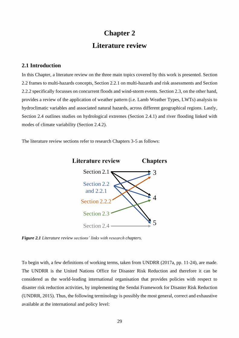
In this Chapter, a literature review on the three main topics covered by this work is presented. Section

2.2 frames to multi-hazards concepts, Section 2.2.1 on multi-hazards and risk assessments and Section

2.2.2 specifically focusses on concurrent floods and wind-storm events. Section 2.3, on the other hand,

provides a review of the application of weather pattern (i.e. Lamb Weather Types, LWTs) analysis to

hydroclimatic variables and associated natural hazards, across different geographical regions. Lastly,

Section 2.4 outlines studies on hydrological extremes (Section 2.4.1) and river flooding linked with

modes of climate variability (Section 2.4.2).

The literature review sections refer to research Chapters 3-5 as follows:

Figure 2.1 Literature review sections’ links with research chapters.

To begin with, a few definitions of working terms, taken from UNDRR (2017a, pp. 11-24), are made.

The UNDRR is the United Nations Office for Disaster Risk Reduction and therefore it can be

considered as the world-leading international organisation that provides policies with respect to

disaster risk reduction activities, by implementing the Sendai Framework for Disaster Risk Reduction

(UNDRR, 2015). Thus, the following terminology is possibly the most general, correct and exhaustive

available at the international and policy level:

Section 2.1

Section 2.2

and 2.2.1

Section 2.2.2

Section 2.3

Section 2.4

3

4

5

Literature review Chapters

30

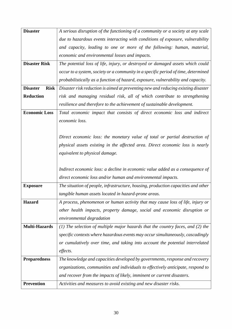
Disaster A serious disruption of the functioning of a community or a society at any scale

due to hazardous events interacting with conditions of exposure, vulnerability

and capacity, leading to one or more of the following: human, material,

economic and environmental losses and impacts.

Disaster Risk The potential loss of life, injury, or destroyed or damaged assets which could

occur to a system, society or a community in a specific period of time, determined

probabilistically as a function of hazard, exposure, vulnerability and capacity.

Disaster Risk

Reduction

Disaster risk reduction is aimed at preventing new and reducing existing disaster

risk and managing residual risk, all of which contribute to strengthening

resilience and therefore to the achievement of sustainable development.

Economic Loss Total economic impact that consists of direct economic loss and indirect

economic loss.

Direct economic loss: the monetary value of total or partial destruction of

physical assets existing in the affected area. Direct economic loss is nearly

equivalent to physical damage.

Indirect economic loss: a decline in economic value added as a consequence of

direct economic loss and/or human and environmental impacts.

Exposure The situation of people, infrastructure, housing, production capacities and other

tangible human assets located in hazard-prone areas.

Hazard A process, phenomenon or human activity that may cause loss of life, injury or

other health impacts, property damage, social and economic disruption or

environmental degradation

Multi-Hazards (1) The selection of multiple major hazards that the country faces, and (2) the

specific contexts where hazardous events may occur simultaneously, cascadingly

or cumulatively over time, and taking into account the potential interrelated

effects.

Preparedness The knowledge and capacities developed by governments, response and recovery

organizations, communities and individuals to effectively anticipate, respond to

and recover from the impacts of likely, imminent or current disasters.

Prevention Activities and measures to avoid existing and new disaster risks.

31

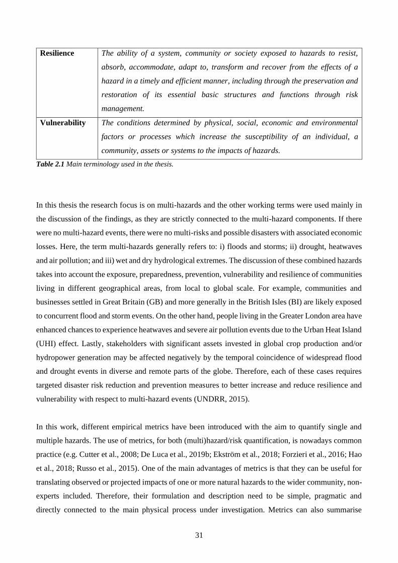
Resilience The ability of a system, community or society exposed to hazards to resist,

absorb, accommodate, adapt to, transform and recover from the effects of a

hazard in a timely and efficient manner, including through the preservation and

restoration of its essential basic structures and functions through risk

management.

Vulnerability The conditions determined by physical, social, economic and environmental

factors or processes which increase the susceptibility of an individual, a

community, assets or systems to the impacts of hazards.

Table 2.1 Main terminology used in the thesis.

In this thesis the research focus is on multi-hazards and the other working terms were used mainly in

the discussion of the findings, as they are strictly connected to the multi-hazard components. If there

were no multi-hazard events, there were no multi-risks and possible disasters with associated economic

losses. Here, the term multi-hazards generally refers to: i) floods and storms; ii) drought, heatwaves

and air pollution; and iii) wet and dry hydrological extremes. The discussion of these combined hazards

takes into account the exposure, preparedness, prevention, vulnerability and resilience of communities

living in different geographical areas, from local to global scale. For example, communities and

businesses settled in Great Britain (GB) and more generally in the British Isles (BI) are likely exposed

to concurrent flood and storm events. On the other hand, people living in the Greater London area have

enhanced chances to experience heatwaves and severe air pollution events due to the Urban Heat Island

(UHI) effect. Lastly, stakeholders with significant assets invested in global crop production and/or

hydropower generation may be affected negatively by the temporal coincidence of widespread flood

and drought events in diverse and remote parts of the globe. Therefore, each of these cases requires

targeted disaster risk reduction and prevention measures to better increase and reduce resilience and

vulnerability with respect to multi-hazard events (UNDRR, 2015).

In this work, different empirical metrics have been introduced with the aim to quantify single and

multiple hazards. The use of metrics, for both (multi)hazard/risk quantification, is nowadays common

practice (e.g. Cutter et al., 2008; De Luca et al., 2019b; Ekström et al., 2018; Forzieri et al., 2016; Hao

et al., 2018; Russo et al., 2015). One of the main advantages of metrics is that they can be useful for

translating observed or projected impacts of one or more natural hazards to the wider community, non-

experts included. Therefore, their formulation and description need to be simple, pragmatic and

directly connected to the main physical process under investigation. Metrics can also summarise

32

complex processes purely defined on a mathematical level, for example in the phase-space, and at the

same time provide information about the dynamics of compound hazards (De Luca et al., 2019b;

Faranda et al., 2017a; Messori et al., 2017). There is therefore hope that metrics will be eventually

used by stakeholders and public agencies to better prepare, communicate and adapt to

(multi)hazards/risks. Possible disadvantages of metrics could be their simplicity, i.e. the fact that

within their formulation there could be processes and mechanisms not quantified or neglected, and

also the possibility that there could be many used to describe the same process. When designing a

metric it is therefore important to consider: i) who may be interested in using the metric; ii) if there are

already other metrics available in the literature that quantify the physical process under investigation;

iii) that the metric is not difficult to interpret; iv) and that directly quantifies the (multi)hazards. In

conclusion, the design of a metric is a trade-off between simplicity and correct representation of the

(multi)hazards. If it is too simple it may be very easy to be understood by end-users, but it may not be

rigorous enough to present the physical process and vice-versa. A similar trade-off is relevant when

considering data belonging to different spatial and time scales.

Indeed, this thesis addresses the topic of multi-hazards with a set of investigations (Chapters 3-5)

spanning different spatial and time scales. Therefore, multi-hazards occurring at catchment, regional

and global geographical scales were investigated by making use of both observations and climate

model projections up to 2100. A clear benefit when looking at small-scale geographical areas is that

the level of detail one can obtain is much higher compared to regional or global analyses. Thus, the

information gained can inform local communities and stakeholders with a smaller level of uncertainty

compared to larger-scale analysis. For example, in Chapter 3 the river basins (even the very small

ones) involved in widespread flooding linked with extra-tropical cyclones (ETCs) in GB are clearly

identified. This could have been much more difficult to detect if, for example, the analysis was

conducted by making use of a global hydrological model with a spatial horizontal resolution of 2.5deg

x 2.5deg. On the other hand, a coarser spatial resolution has the benefit to provide a global picture of

a given multi-hazards process, with a manageable computational cost. For example, in Chapter 5

concurrent wet and dry hydrological extremes have been explored at the global scale, and although

localised details of these concurrent extremes cannot be obtained, one has a global picture of where

and when they co-occurred. Thus, such information may not be highly useful for a local community

(e.g. village, business or farm) but it can be appreciated by international organizations and global

stakeholders. A similar concept applies also to time-scales. Here, a finer temporal resolution of, for

example, hourly instead of daily observations can be necessary for detecting a specific physical process

(e.g. storm surges or wind gusts). Whereas the output of a climate model, while not providing the exact

33

information for a given day in the future, informs us about the possible general trends of the chosen

variable at seasonal, annual or decadal scales. In conclusion, both small and large-scale geographical

analyses and finer and coarser temporal resolutions have pros and cons, and the choice of one instead

of the other depends respectively on the targeted end-user and physical process under investigation. In

this thesis it is shown that multi-hazards research can, and needs to, be tackled at both small and large

geographical scales, by looking at both observations and future climate projections.

2.2 Multi-hazards

Within the academic community, the concept of natural hazards acting independently has now changed

to a multi-hazard or compound events approach (UNDRR, 2015; Zscheischler et al., 2018), and

although with slower timing this is occurring in the governance sector as well. Thus, a more holistic,

multi-hazards perspective is emerging with importance especially for future projections of potential

high-impact events and for bridging the gap between physical/social scientists, engineers, climate

impact modellers and stakeholders (AghaKouchak et al., 2018; Zscheischler et al., 2018).

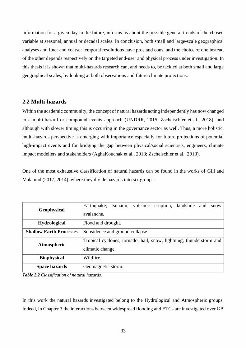
One of the most exhaustive classification of natural hazards can be found in the works of Gill and

Malamud (2017, 2014), where they divide hazards into six groups:

Geophysical Earthquake, tsunami, volcanic eruption, landslide and snow

avalanche.

Hydrological Flood and drought.

Shallow Earth Processes Subsidence and ground collapse.

Atmospheric Tropical cyclones, tornado, hail, snow, lightning, thunderstorm and

climatic change.

Biophysical Wildfire.

Space hazards Geomagnetic storm.

Table 2.2 Classification of natural hazards.

In this work the natural hazards investigated belong to the Hydrological and Atmospheric groups.

Indeed, in Chapter 3 the interactions between widespread flooding and ETCs are investigated over GB

34

(De Luca et al., 2017), whereas in Chapter 4 past and future weather pattern persistence in the BI is

linked with flood-wind and heatwave-air pollution hazards (De Luca et al., 2019a). Lastly, in Chapter

5 a global analysis of concurrent wet and dry hydrological extremes with also links to modes of climate

variability is presented (De Luca et al., 2019c).

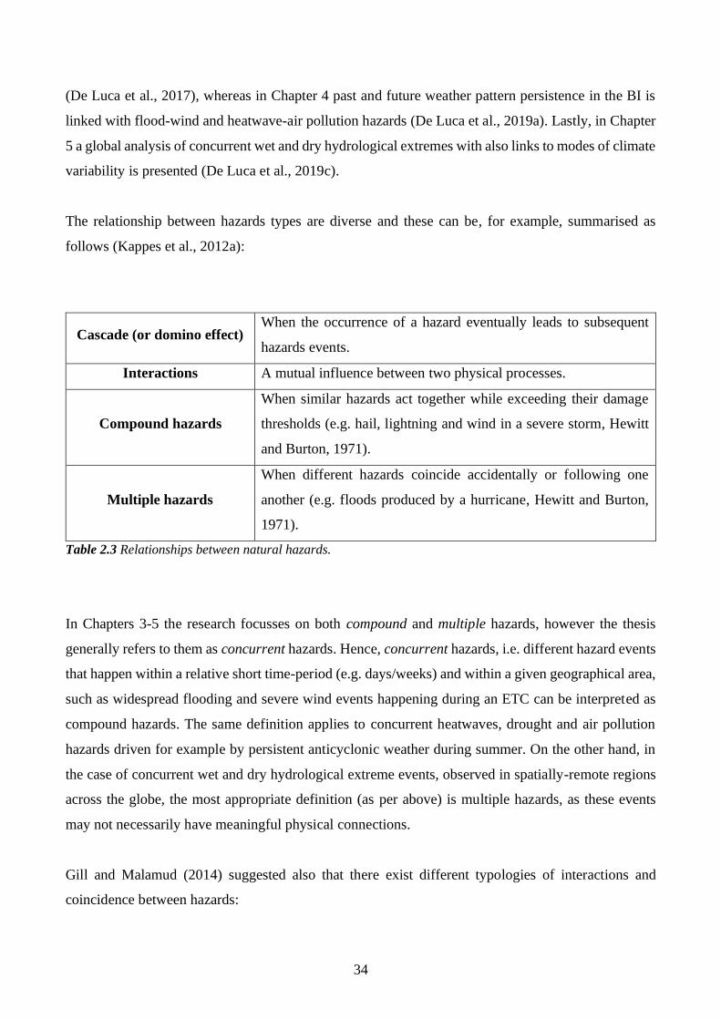
The relationship between hazards types are diverse and these can be, for example, summarised as

follows (Kappes et al., 2012a):

Cascade (or domino effect) When the occurrence of a hazard eventually leads to subsequent

hazards events.

Interactions A mutual influence between two physical processes.

Compound hazards

When similar hazards act together while exceeding their damage

thresholds (e.g. hail, lightning and wind in a severe storm, Hewitt

and Burton, 1971).

Multiple hazards

When different hazards coincide accidentally or following one

another (e.g. floods produced by a hurricane, Hewitt and Burton,

1971).

Table 2.3 Relationships between natural hazards.

In Chapters 3-5 the research focusses on both compound and multiple hazards, however the thesis

generally refers to them as concurrent hazards. Hence, concurrent hazards, i.e. different hazard events

that happen within a relative short time-period (e.g. days/weeks) and within a given geographical area,

such as widespread flooding and severe wind events happening during an ETC can be interpreted as

compound hazards. The same definition applies to concurrent heatwaves, drought and air pollution

hazards driven for example by persistent anticyclonic weather during summer. On the other hand, in

the case of concurrent wet and dry hydrological extreme events, observed in spatially-remote regions

across the globe, the most appropriate definition (as per above) is multiple hazards, as these events

may not necessarily have meaningful physical connections.

Gill and Malamud (2014) suggested also that there exist different typologies of interactions and

coincidence between hazards:

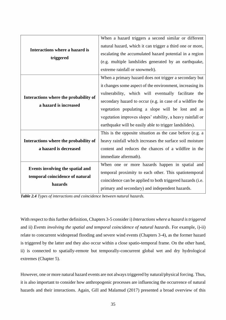
35

Interactions where a hazard is

triggered

When a hazard triggers a second similar or different

natural hazard, which it can trigger a third one or more,

escalating the accumulated hazard potential in a region

(e.g. multiple landslides generated by an earthquake,

extreme rainfall or snowmelt).

Interactions where the probability of

a hazard is increased

When a primary hazard does not trigger a secondary but

it changes some aspect of the environment, increasing its

vulnerability, which will eventually facilitate the

secondary hazard to occur (e.g. in case of a wildfire the

vegetation populating a slope will be lost and as

vegetation improves slopes’ stability, a heavy rainfall or

earthquake will be easily able to trigger landslides).

Interactions where the probability of

a hazard is decreased

This is the opposite situation as the case before (e.g. a

heavy rainfall which increases the surface soil moisture

content and reduces the chances of a wildfire in the

immediate aftermath).

Events involving the spatial and

temporal coincidence of natural

hazards

When one or more hazards happen in spatial and

temporal proximity to each other. This spatiotemporal

coincidence can be applied to both triggered hazards (i.e.

primary and secondary) and independent hazards.

Table 2.4 Types of interactions and coincidence between natural hazards.

With respect to this further definition, Chapters 3-5 consider i) Interactions where a hazard is triggered

and ii) Events involving the spatial and temporal coincidence of natural hazards. For example, i)-ii)

relate to concurrent widespread flooding and severe wind events (Chapters 3-4), as the former hazard

is triggered by the latter and they also occur within a close spatio-temporal frame. On the other hand,

ii) is connected to spatially-remote but temporally-concurrent global wet and dry hydrological

extremes (Chapter 5).

However, one or more natural hazard events are not always triggered by natural/physical forcing. Thus,

it is also important to consider how anthropogenic processes are influencing the occurrence of natural

hazards and their interactions. Again, Gill and Malamud (2017) presented a broad overview of this

36

subject, as they investigated 18 (non-malicious) human process types influencing 21 natural hazards

and their interactions. In this thesis the direct human influence on natural hazards is not quantified,

therefore the following description is intended to only provide a general overview of the human

processes involved.

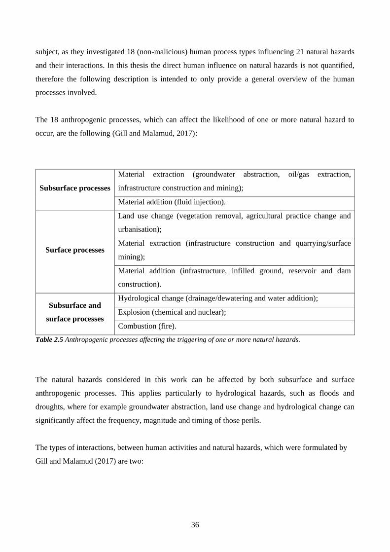
The 18 anthropogenic processes, which can affect the likelihood of one or more natural hazard to

occur, are the following (Gill and Malamud, 2017):

Subsurface processes

Material extraction (groundwater abstraction, oil/gas extraction,

infrastructure construction and mining);

Material addition (fluid injection).

Surface processes

Land use change (vegetation removal, agricultural practice change and

urbanisation);

Material extraction (infrastructure construction and quarrying/surface

mining);

Material addition (infrastructure, infilled ground, reservoir and dam

construction).

Subsurface and

surface processes

Hydrological change (drainage/dewatering and water addition);

Explosion (chemical and nuclear);

Combustion (fire).

Table 2.5 Anthropogenic processes affecting the triggering of one or more natural hazards.

The natural hazards considered in this work can be affected by both subsurface and surface

anthropogenic processes. This applies particularly to hydrological hazards, such as floods and

droughts, where for example groundwater abstraction, land use change and hydrological change can

significantly affect the frequency, magnitude and timing of those perils.

The types of interactions, between human activities and natural hazards, which were formulated by

Gill and Malamud (2017) are two:

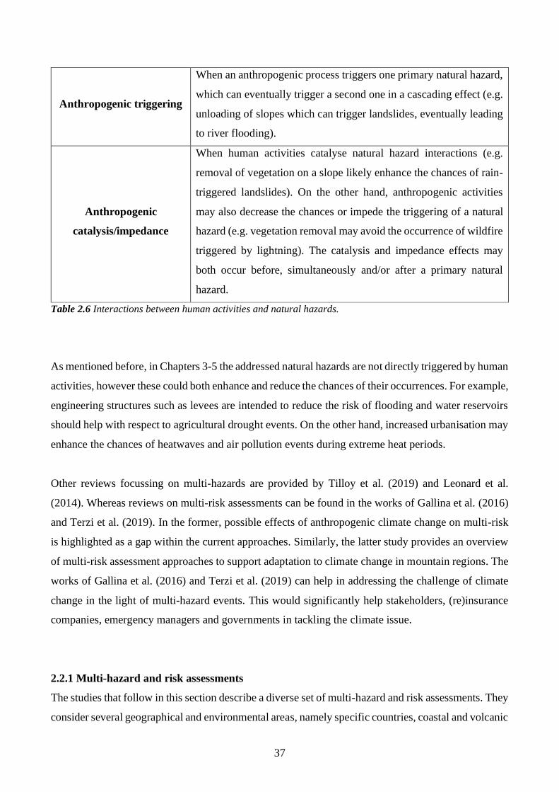
37

Anthropogenic triggering

When an anthropogenic process triggers one primary natural hazard,

which can eventually trigger a second one in a cascading effect (e.g.

unloading of slopes which can trigger landslides, eventually leading

to river flooding).

Anthropogenic

catalysis/impedance

When human activities catalyse natural hazard interactions (e.g.

removal of vegetation on a slope likely enhance the chances of rain-

triggered landslides). On the other hand, anthropogenic activities

may also decrease the chances or impede the triggering of a natural

hazard (e.g. vegetation removal may avoid the occurrence of wildfire

triggered by lightning). The catalysis and impedance effects may

both occur before, simultaneously and/or after a primary natural

hazard.

Table 2.6 Interactions between human activities and natural hazards.

As mentioned before, in Chapters 3-5 the addressed natural hazards are not directly triggered by human

activities, however these could both enhance and reduce the chances of their occurrences. For example,

engineering structures such as levees are intended to reduce the risk of flooding and water reservoirs

should help with respect to agricultural drought events. On the other hand, increased urbanisation may

enhance the chances of heatwaves and air pollution events during extreme heat periods.

Other reviews focussing on multi-hazards are provided by Tilloy et al. (2019) and Leonard et al.

(2014). Whereas reviews on multi-risk assessments can be found in the works of Gallina et al. (2016)

and Terzi et al. (2019). In the former, possible effects of anthropogenic climate change on multi-risk

is highlighted as a gap within the current approaches. Similarly, the latter study provides an overview

of multi-risk assessment approaches to support adaptation to climate change in mountain regions. The

works of Gallina et al. (2016) and Terzi et al. (2019) can help in addressing the challenge of climate

change in the light of multi-hazard events. This would significantly help stakeholders, (re)insurance

companies, emergency managers and governments in tackling the climate issue.

2.2.1 Multi-hazard and risk assessments

The studies that follow in this section describe a diverse set of multi-hazard and risk assessments. They

consider several geographical and environmental areas, namely specific countries, coastal and volcanic

38

areas, cities and continent-scale assessments. They also review empirical metrics, physical

mechanisms, social and economic impacts of multi-hazards, by taking examples from different

countries and eventually concentrating the focus on the United Kingdom (UK).

During the past decade, there was a large focus on multi-hazard risk assessments which, as per

definition, consider the exposure, vulnerability and multi-hazard interactions to define risk. They have

been performed nationally as in the case of China (Zhou et al., 2015), where five major hazards were

evaluated (earthquakes, floods, droughts, low temperatures/snow and gale/hail). Or for a single region

(Liu et al., 2017), where a specific model of interacting hazards, based on a Bayesian network, was

developed in order to calculate the expected multi-hazard occurrences and losses in terms of impacts

on society, environment and economy.

Multi-hazard assessments have also been undertaken for coastal areas, which contain large

concentrations of people and infrastructure that are exposed to natural hazards such as tsunamis, storm

surges and tropical cyclones. Rosendahl Appelquist and Halsnæs (2015) present a global analysis

based on the so called Coastal Hazard Wheel (CHW) system and by considering the impact of climate

change and hazards such as ecosystem disruption, gradual inundation, salt water intrusion, erosion and

flooding. Regional coastal studies have been undertaken, for example in Goa, India (Kunte et al., 2014)

or the Ganges deltaic coast of Bangladesh (Ashraful Islam et al., 2016), where a coastal vulnerability

index (CVI) was developed with the aid of geospatial techniques (i.e. remote sensing and GIS). The

latter also applied a multi-hazard vulnerability assessment in the southeast coast of India (Mahendra

et al., 2011), one of the most impacted by the 2004 Indian Ocean tsunami. Such studies prove the

utility and associated applicability of empirical metrics, which are able to capture diverse

characteristics of multi-hazards and that can eventually benefit the overall resilience and disaster risk

reduction policies implemented by local and regional policy makers.

The types of natural hazards are numerous and not all of them are strictly connected to the hydrological

cycle or to large-scale atmospheric configurations (see Table 2.5). As an example, volcanically active

areas also provided interest with respect to multi-hazard risk assessments. For instance, assessments

were performed for Mount Cameroon in Africa (Thierry et al., 2008) and El Misti in Peru (Sandri et

al., 2014). In these areas, hazards such as volcanic eruptions (e.g. pyroclastic density currents, lava

flows, lahars, tephra fall and ballistic ejecta), landslides, earthquakes pose a significant threat to

populations living nearby.

39

Multi-risk assessments have also been performed for individual cities. For example, one project

evaluated the exposure of Sydney (Australia) to tsunamis, storms and sea level rise through a

probabilistic approach (Dall’Osso et al., 2014). A complete risk assessment can be found for two Hong

Kong districts (Johnson et al., 2016) and for the city of Conceptión (Chile) (Araya-Muñoz et al., 2017),

where in the latter a methodology based on fuzzy logic modelling was developed. Also, a further and

more complex three-hazard scenario (storms, floods and earthquakes) was considered for the city of

Cologne (Germany), where a multi-risk assessment was applied to predict direct economic losses to

buildings and their contents (Grünthal et al., 2006). Investigating multi-hazards at such local scales

proves the transversal characteristic of the topic, which indeed can range from local to continental and

even global scales. Multiple natural hazards impacting highly-dense populated cities, via the above-

mentioned hazards of for example by a combination of heatwaves and severe air pollution episodes,

linked to persistent anticyclonic or blocked atmospheric conditions, can result in significant societal

losses. An example of this can be drawn from the 2003 and 2010 summer heatwaves in Europe

(Barriopedro et al., 2011; Le Tertre et al., 2006; Stott et al., 2004).

Finally, continental multi-hazard assessment was performed for Europe in the light of climate change

(Forzieri et al., 2016). The investigation considers an ensemble of General Circulation Model-Regional

Climate Model (GCM-RCM) climate projections, under the A1B emission scenario, to deliver changes

in the frequency of multiple natural hazards, such as heat and cold waves, river and coastal flooding,

droughts, wildfires and windstorms. Time periods considered were the historical (1980-2010) and the

three future periods up to 2100, namely 2020s (2011-2040), 2050s (2041-2070) and 2080s (2071-

2100). Here, several metrics able to quantify the physical impacts of each hazards, were developed

and applied, as for example the Heat Wave Magnitude Index daily (HWMId) (Russo et al., 2015).

Moreover, the return periods, along with the exposure (defined as the Expected Annual Fraction

Exposed (EAFE)) associated with the natural hazards were also computed. And lastly, a new multi-

hazards metric, that quantifies the annual exposure from all the hazards combined, was also introduced

as the Overall Exposure Index (OEI). Forzieri et al. (2016) prove that multi-hazard metrics can be

useful for quantifying future climate change impacts at the continental scale.

Within the UK recent studies have started to apply multi-hazards concepts. For instance, weather-

driven hazards such as floods, droughts, windstorms and shrink-swell subsidence were found to

interact physically, leading also to compound economic damages (Collet et al., 2018; De Luca et al.,

2017; Hillier et al., 2015; Visser-Quinn et al., 2019). Multi-basin (i.e. widespread) floods in GB are

shown to be driven by ETCs – the latter identified through Very Severe Gales (VSGs), cyclonic LWTs

40

and atmospheric rivers (ARs) (De Luca et al., 2017). This is consistent with ARs contributing to the

10 largest winter flood events in four GB basins considered independently from each other (i.e. single-

basin floods) (Lavers et al., 2013, 2011). Shrink-swell episodes occur between very wet and very dry

hydrological periods and thus they are the result of a combination of hazards. These events were

identified from subsidence insurance claims within the 1987-2008 period and were also linked to

historical climate data in south-eastern England (Harrison et al., 2012). Findings show that for

precipitation above 394mm within a given past 2-year period, insurance claims were lower in

frequency, whereas for precipitation lower than 350mm the incidence was higher. Interacting UK

hydro-hazards, defined as floods and droughts, were also quantified by considering their magnitude,

frequency and duration in both model observations and future projections, making possible the

identification of hydro-hazard hotspots (Collet et al., 2018; Visser-Quinn et al., 2019). Indeed, Collet

et al. (2018) found that future hotspots are likely to develop along the western coast of England and

Wales and over north-eastern Scotland during, winter and autumn respectively for floods and droughts.

Similarly, Visser-Quinn et al. (2019) showed that spatio-temporal compound hydro-hazards hotspots

lie in north-eastern Scotland and south-western UK. These findings are therefore likely to be relevant

for water management companies, with related socio-economic implications. Starting from these two

national-scale studies on concurrent floods and droughts events one can also expand the proposed

analyses on a larger geographical scale, such as Europe or even the entire globe. This could be achieved

by making use of global observational datasets, such as the Palmer Drought Severity Index (PDSI)

(Dai et al., 2004; Palmer, 1965), along with future climate projections (e.g. Eyring et al., 2016; Taylor

et al., 2011). The resulting findings may therefore help hedging losses by stakeholders and

(re)insurance companies with global assets invested for example in hydropower (Ng et al., 2017;

Turner et al., 2017) and crops production (Leng and Hall, 2019; Zampieri et al., 2017).

2.2.2 Storm-driven floods

Flooding events in the UK are known to cause severe impacts in terms of economic and social damages

(CCRA, 2016). These events are naturally associated with the passage of ETCs impacting the BI during

late autumn and winter seasons (De Luca et al., 2017). Hence, these episodes are a combination of

both hydrological and atmospheric processes and can be defined as concurrent hazards, that are also

possibly affected by anthropogenic subsurface and surface processes (Gill and Malamud, 2017, 2014;

Kappes et al., 2012a).

41

In this section, recent examples of exceptional UK storm-driven widespread flooding occurred in the

21st century are summarised. This will provide a relevant review of studies connected to research

Chapter 3 (De Luca et al., 2017), by also highlighting the lack of research conducted with respect to

the quantification of concurrent flood-wind hazards.

Autumn and winter 2000-2001 floods. During this period, the UK experienced the most severe floods

since 1947, during which catchments remained saturated for long periods and severe groundwater

flooding affected southern England (Marsh and Dale, 2002). The widespread flooding was found to

be one of the most extreme episodes in GB within the 1975-2014 period (De Luca et al., 2017). Autumn

2000 was the wettest in England and Wales since records began in 1766 and the flooding episodes

damaged ~10,000 properties, caused service disruption and £1.3 billion of economic losses in England

and Wales (Pall et al., 2011). The physical mechanisms driving the flooding episodes were identified

as westerly circulation patterns and in the passage of diverse frontal systems (Marsh and Dale, 2002)

and ARs (De Luca et al., 2017). Some of the storms were remnants of Atlantic hurricanes, which

brought heavy rainfall that eventually saturated soils, leading to enhanced runoff and flooding. Sea-

surface temperatures (SSTs) also played a role, as the thermal gradient can influence storm activity

over Europe. During autumn 2000, the SST anomaly was very high (2 °C degrees above the monthly

average) which resulted in a sharp south-west to north-east gradient (Marsh and Dale, 2002). This

widespread flooding in England and Wales was also attributed to anthropogenic greenhouse gas

emissions (Pall et al., 2011). Thousands of climate model simulations of autumn 2000 weather were

performed under various greenhouse gas emissions pathways and then integrated into a precipitation-

runoff model for England and Wales. The results showed that in 9 out of 10 cases, greenhouse gas

emissions had increased the likelihood of the autumn 2000 floods by more than 20% and in two runs

by more than 90% (Pall et al., 2011).

Summer 2007 floods in England and Wales. During May-July extreme rainfall hit England and Wales

with no precedent since 1847 and some areas reported flooding more severe than that in 1947. In total,

14 people died, thousands experienced misery as a result of properties being flooded (over 55,000

homes and 6,000 businesses) and insurance claims reached £3 billion pounds (Marsh and Hannaford,

2007). Flash flooding and floodplain inundation were observed from mid-June to the end of July and

the dominant flood-generating mechanisms were three slow-moving low-pressure systems (i.e.

storms) that caused the exceptional precipitation totals. Soil moisture conditions also played a pivotal

role in increasing the likelihood of flooding. Normally, during summer, when there are higher

42

temperatures and evaporation, a Soil Moisture Deficit (smd) reduces the likelihood of flooding. By the

end of April 2007, soils in England and Wales were their driest since 1961 but this situation reversed

completely between May and July, leading to widespread flooding (Marsh and Hannaford, 2007).

Similarly, groundwater levels also contributed to fluvial flooding – in late April 2007 levels were low

across England and Wales, but they increased sharply between the May-July period. Although robust

data on summer storms’ frequency is lacking, links to climate change can still be made, because low-

pressure systems as the ones observed in 2007 have characteristics that belong to the future climate

regime (Marsh and Hannaford, 2007).

Summer 2012 flooding in England and Wales. A similar, but even more exceptional situation led to

flooding in summer 2012. In March 2012, the UK experienced one of the most significant droughts in

a century, which depressed river flows and groundwater levels (Kendon et al., 2013). Then April to

July 2012 were the wettest ever recorded in England and Wales within 250 years, which reversed the

attention from drought to flooding. Synoptic conditions driving the change were identified as low-

pressure systems affecting the northern UK between 2011 and early 2012, leading to water scarcity in

southern GB. From April 2012, the jet stream was more southerly, bringing low-pressure and heavy

rains across the country (Parry et al., 2013). April 2012 was the wettest in the UK since 1910 and the

wettest for England and Wales within a 250-year period. The causes of the reversed conditions (i.e.

drought to flood) reflect the variability of the UK climate. However, robust attributions have not yet

been formulated but they could possibly lie with El Niño Southern Oscillation (ENSO) variability and

global warming (Parry et al., 2013).

Winter of 2013-2014 floods. Several studies have investigated this exceptional winter period for the

UK, which experienced extreme rainfall, fluvial, pluvial, groundwater and coastal flooding due to the

passage of many low-pressure systems (Huntingford et al., 2014; Kendon, 2015; Kendon and

McCarthy, 2015; Knight et al., 2017; Matthews et al., 2014; Muchan et al., 2015; Priestley et al., 2017;

Schaller et al., 2016). In total, 7,000 properties experienced flooding (Muchan et al., 2015) and 18,700

flood insurance claims were made, resulting in £451 million losses in southern England (Schaller et

al., 2016). This winter was the wettest on record since 1910 and the stormiest ever for the UK and

Ireland (Matthews et al., 2014). Various physical explanations have been offered. A strong and

persistent cyclonic atmospheric circulation over the North Eastern Atlantic Ocean, connected to a very

intense North Atlantic jet stream bringing heavy rainfall and wind storms (Knight et al., 2017).

Tropical regions have likely influenced the development of the severe extra-tropical circulation and

the stratospheric polar vortex, which in turn was associated with a strong westerly phase of Quasi-

43

Biennial Oscillation (QBO), which increased the extreme weather conditions (Huntingford et al., 2014;

Knight et al., 2017). Other possible causes were the positive phase of the North Atlantic Oscillation

(NAO), during the 2013-2014 winter, which is known to drive extreme cyclones that eventually bring

high-speed winds and rainfall, leading to flooding in northern Europe (e.g. Hannaford and Marsh,

2008; Pinto et al., 2009). Other possible drivers have been identified including Arctic sea ice extent

and solar activity (Huntingford et al., 2014), although these causes may be less certain as the physical

mechanisms involved are not yet fully understood.

Winter 2015-2016 flooding in the UK. This episode represented another record-breaking period in

terms of weather extremes, with widespread flooding driven by diverse storms impacting the UK

(Barker et al., 2016; Burt, 2016; Burt et al., 2016; Burt and Kendon, 2016; McCarthy et al., 2016).

Around 16,000 properties flooded in England during December, causing negative impacts on homes,

businesses, industry, transport and agriculture. Nine storms (or ETCs) were the cause of the

widespread flooding, with storm Desmond being the most powerful and impacting the northwest of

England and southern Scotland, with significant damages reported in Cumbria (Barker et al., 2016;

Burt et al., 2016; McCarthy et al., 2016). Monthly rainfall records were broken during winter 2015 in

the UK, with no precedent since records began in 1910 and quantities up to four times the normal in

western and northern areas (Wilby and Barker, 2016). December 2015 was also characterised by

exceptionally mild temperatures, which meant that high altitude precipitation fell as rain instead of

snow, contributing to more rapid runoff from headwaters. Possible explanations for this remarkable

winter are the 2015 El Niño event in the Pacific Ocean connected with a positive phase of the NAO.

Also human influence, in terms of global warming, may have contributed to the extreme winter

precipitation for the UK with circulation patterns similar to winter 2013-2014 (McCarthy et al., 2016).

The above examples of recent widespread flooding episodes give vital insights into the storm-

dominating mechanisms that are driving such perils. However, apart from the work presented here in

Chapter 3 (De Luca et al., 2017), previous studies do not explicitly quantify links between widespread

flooding and ETCs. Hence, although clear and thorough physical explanations about the role of the

atmosphere in driving such flooding were made, there is a lack of, for example, a record of widespread

flooding events linked with ETCs. As proved by the studies cited above, ETCs, i.e. synoptic (or large-

scale) low-pressure weather systems occurring in the midlatitudes especially during the winter season,

create highly-favourable conditions for flooding in the UK. Apart from severe gales, possibly resulting

in property damages and storm surges in coastal areas, they can also bring prolonged and high-intensity

rainfall, with associated river flooding (De Luca et al., 2017; Lavers et al., 2011). The UK is situated

44

beneath the North Atlantic storm track and represents (along with Ireland) the first country impacted

by the passage of ETCs (Matthews et al., 2016b), that can subsequently affect central Europe (Donat

M. G., Leckebusch G. C., Pinto J. G., 2010; Priestley et al., 2017). Since ETCs can continue to

strengthen after landfall, their impacts may extend to a much larger physical and financial scale than

the UK alone (Donat M. G., Leckebusch G. C., Pinto J. G., 2010).

2.3 Weather patterns

In this section the literature review’s focus changes to weather patterns and their links with

hydroclimatic variables and natural hazards over the BI and other regions mostly spread across the

European continent. This review has the intent to introduce Chapter 4, which focusses on a quantitative

and qualitative analysis of multi-hazards derived from weather patterns in the BI (De Luca et al.,

2019a). Thus, the geographical domain expands from catchment/national to regional scale.

Daily atmospheric pressure patterns for the British Isles have been categorised according to the system

of LWTs (Lamb, 1972). This classification was originally subjective, meaning that daily weather

patterns were assigned manually after inspection of weather charts. A few years after the first

subjective classification of LWTs (Lamb, 1972), an objective method to detect daily atmospheric

circulation following LWTs was developed (Jenkinson and Collison, 1977). Eventually, both the

subjective and objective approach were compared (Jones et al., 1993) and objective LWTs were also

derived from reanalyses products (Jones et al., 2013). The main novelty of the objective classification

scheme was that it uses grid-point daily mean sea-level-pressure (SLP) analysis for a fixed observation

time (such as 00:00 or 12:00 UTC) (Jones et al., 2014). Both the subjective and objective classification

schemes yield 27 LWTs comprised of two synoptic (A and C), five purely directional (W, NW, E, N,

and S), 19 hybrid combinations of synoptic and pure directional (e.g. CNW, CSE and AE), and one

unclassified (U) type (Jenkinson and Collison, 1977; Jones et al., 1993). A current unsolved difference

between the objective and subjective schemes is that the former does not show a reduction in the daily

W-type count since the 1920s, whereas such a feature was evident in several of Lamb’s works (Jones

et al., 2014).

For the seven main LWTs, acronyms correspond to the following:

A = anticyclonic

45

C = cyclonic

W = westerly

NW = north-westerly

E = easterly

N = northerly

S = southerly

Over time, as shown below, LWTs attracted much interest. Firstly, because of their strong association

(or significant correlations) with other meteorological variables, such as temperature and precipitation

(Jones et al., 2014). Secondly, because the objective classification method can be applied not only to

the BI but also to other regions of interest within the mid-to-high latitudes (Jones et al., 2013). Thus,

a large body of literature addresses LWTs in the UK, Ireland, Sweden, Netherlands, Poland, Iberian

peninsula, Spain, Portugal, Mediterranean region, Greece, Turkey, Morocco, Arabian peninsula, China

and more broadly across the European continent. These diverse studies are reviewed below for each

geographical domain, so that a comprehensive narrative on the diverse uses of LWTs is provided. This

will also confirm the vast applicability of the objective LWTs method, not only with respect to different

geographical areas, but also to a diverse set of hydroclimatic and atmospheric variables.

For the BI, LWTs were linked to extreme precipitation totals in the 1870s driven by cyclonic weather

patterns (Burt et al., 2015). During these heavy rainfall events, a low frequency of anticyclonic and

westerly types were also recorded, with the latter contributing to significant rainfall totals mainly in

the uplands and north-western coastal regions. Another study looked at relationships between weather

patterns and the NAO and the oxygen isotopic composition of rainfall, which is fundamental for

paleoclimate reconstruction (Tyler et al., 2016). They found an association between the oxygen isotope

and LWTs, especially with the cyclonic types. Other work examined the climatology of cyclones

during the period 1871 to 2012 (Matthews et al., 2016b). They found that such weather types drive

seasonal precipitation totals, exhibit interannual and multi-decadal variability, exhibit no increasing

trend in frequency and storminess, although cyclone intensity has increased especially during the

winter season (Matthews et al., 2016b).

LWTs have also been used to downscale GCMs outputs, such as monthly means, persistence and

interannual variability of rainfall (Conway and Jones, 1998). Other research has linked ground-level

ozone concentrations to variations in atmospheric circulation (O’Hare and Wilby, 1995). Peak ozone

concentrations are observed during anticyclonic and easterly days, whereas westerly and cyclonic

46

LWTs increase the mean ozone concentration at remote sites due to turbulent mixing processes. In one

of the first studies of its kind, Hulme et al. (1993) used LWTs to validate two GCM control simulations

against their relative observations of weather type, finding that both GCMs produced too many

cyclonic types during winter and that summer temperature variability over the region is not driven by

changes in weather patterns. Similarly, a recent study of future LWTs under Representative

Concentration Pathway (RCP) 8.5 showed that westerly advection may become more frequent by the

end of the 21st-century, whereas southerly and northerly weather types are projected to reduce in

frequency (Stryhal and Huth, 2018).

Numerous other studies focus on the smaller domain of the UK (e.g. Blenkinsop et al., 2015; Burt and

Ferranti, 2012; De Luca et al., 2017; Fowler et al., 2000; Fowler and Kilsby, 2002b, 2002a; Jones et

al., 2016; Neal and Phillips, 2011; Pattison and Lane, 2012; Pope et al., 2015, 2014, 2016; Richardson

et al., 2018; Wetterhall et al., 2012; Wilby, 1998, 1995, 1994, 1993; Wilby et al., 1997; Zhang et al.,

2014), with a particular emphasis on precipitation. For example, south-westerly and easterly LWTs

are found to yield respectively the largest and smallest amount of daily rainfall in Cumbria (Neal and

Phillips, 2011). Another study relates low-frequency/high-magnitude rainfall events in central and

southern England to LWTs and found three distinct weather-type clusters (i.e. cyclonic, directional

and anticyclonic) that could eventually be used to construct a simple weather model (Wilby, 1998).

Moreover, long rainfall records across the north of England show that rising winter rainfall is due to

an increase in westerly weather types (Burt and Ferranti, 2012; Fowler and Kilsby, 2002a), whereas

declining summer precipitation is linked to a reduction of cyclonic days (Burt and Ferranti, 2012) as

well as westerly LWTs over the Yorkshire region (Fowler and Kilsby, 2002a). LWTs were also linked

to two sites in central and southern England, then simulation by matrices of transition probabilities

along with series of daily and annual precipitation totals, resulted in better estimation of the latter when

compared to a simple rainfall generator model (Wilby, 1995). A similar approach, by the same author,

was also used to build a stochastic model generator of LWTs and rainfall, which reproduces the

different temporal resolutions of rainfall totals (i.e. daily, monthly and annual), with intended

applications to climate change impact assessments (Wilby, 1994).

Other UK studies have linked weather types with air quality and pollution (Pope et al., 2016; 2015;

2014; Zhang et al., 2014). For example, Pope et al. (2015; 2014) examined weather patterns and the

tropospheric NO2 column. They found that cyclonic conditions show higher seasonality compared with

anticyclonic weather patterns, with the former leading to NO2 reduction compared to the latter, during

which its accumulation is enhanced. Moreover, LWTs were also associated with surface ozone, that

47

can lead to health problems, and results show that anticyclonic and easterly LWTs enhance ozone

concentrations over the UK, whereas cyclonic and westerly weather patterns lower ozone, due to

advection and replacement with clean air from the North Atlantic (Pope et al., 2016). LWTs have also

linked to multi-basin flooding events in GB, with cyclonic and westerly types driving such episodes

(De Luca et al., 2017). Another analysis based on a single river basin, showed that extreme floods

were generated by cyclonic and westerly types over the 1976-2007 period (Pattison and Lane, 2012).

Finally, LWTs have been applied to drought analysis in Yorkshire (Fowler and Kilsby, 2002b) and

used to benchmark a new set of weather patterns developed by the Met Office through a national-scale

drought analysis (Richardson et al., 2018).

In Sweden, much LWTs research has focussed on air quality assessments (Grundström et al., 2015a,

2015b; Pleijel et al., 2016; Tang et al., 2009). For instance, in Gothenburg air pollutants such as NO2,

CO, PM10 and O3 along with deposition of nitrate, ammonium and sulphate were correlated with annual

LWTs frequencies and results show statistically significant values, proving the existence of robust

links between LWTs and pollutants (Pleijel et al., 2016). Another study in Gothenburg examined the

connections between LWTs and the particle number concentrations (PNC), NOx, NO2 and PM10,

concluding that the anticyclonic, north-westerly, northerly and north-easterly weather patterns are the

high-risk categories with higher concentrations of pollutants (Grundström et al., 2015a). Moreover,

partially in accord with the above findings, in southern Sweden it was found that ozone levels are

higher during anticyclonic, south-eastern/eastern and south-western/southern weather patterns (Tang

et al., 2009) and NO2 concentrations higher during anticyclonic, north-westerly and northerly LWTs

(Grundström et al., 2015b). Lower NO2 levels were found during easterly, southerly, south-westerly

and westerly types (Grundström et al., 2015b).

A national-scale study of precipitation events in Sweden found that cyclonic LWTs accounted for

~70% of extreme events but only ~45% for non-extreme ones, with lower westerly and stronger

southerly winds favouring extremes (Hellström, 2005). Observed temperatures across southwestern

Sweden during winter were also related to LWTs during January (Chen, 2000). The work showed that

westerly weather types favour positive temperature anomalies and south-westerly patterns favour

positive extremes (i.e. higher temperatures), whereas anticyclonic conditions are related with negative

and extreme negative temperature anomalies. This anomaly and extreme temperature patterns are

expected for a winter month such as January, as for example anticyclonic conditions bring clear skies

with also the possibility of blocking events, that during winter eventually result in severe temperature

drops due to the lack of thermal radiation being trapped by clouds. On the other hand, during summer

48

anticyclonic weather (and hence blocking) is associated with extreme heat events, possibly leading to

concurrent heatwaves, droughts and air pollution episodes.

Within the Iberian Peninsula several studies have applied LWTs to precipitation (Cortesi et al., 2014,

2013; Domínguez-Castro et al., 2015; Paredes et al., 2006). For example, Cortesi et al. (2014) and

Paredes et al. (2006) clearly show that much of the rainfall falling into the Iberian peninsula is driven

by few LWTs, with the westerly, south-westerly and cyclonic being the most predominant ones.

Moreover, the links between weather types and rainfall seem to be stronger during winter and in the

western areas of the peninsula. On the Mediterranean coast precipitation is driven by easterly types,

whereas in the Cantabrian coast northerly and north-westerly patterns dominate and cyclonic LWTs

although result to be the less frequent are the most efficient in generating precipitation (Cortesi et al.,

2014). Paredes et al. (2006) looked at the decline in rainfall during March and showed that cyclonic,

westerly and south-westerly LWTs are declining in frequency and are accompanied by an increase in

anticyclonic pattern, proving that over time low pressure systems are becoming less frequent. LWTs

were also successfully used as predictor variables by Cortesi et al. (2013) and Ramos et al. (2010) for

modelling national-scale monthly precipitation across the peninsula and linked with modes of climate

variability in the northwest. Ramos et al. (2010) also show that the NAO is highly correlated with

cyclonic and anticyclonic weather types, the East Atlantic (EA) pattern with the south-westerly LWT,

the Eurasian pattern 1 (EA/WR) with westerly and north-westerly types and the Scandinavian (SCA)

pattern shows negative correlation with anticyclonic and positive correlation with cyclonic circulation

types. Lorenzo et al. (2011) looked at 21st-century changes in atmospheric circulation in the north-

western Iberian Peninsula and projected a decrease in the frequency of cyclonic, westerly and south-

westerly LWTs during spring, summer and autumn, but an increase in anticyclonic patterns in autumn.

Peña-Angulo et al. (2016) also explained with LWTs observed monthly mean maximum and minimum

temperatures over the 1950-2010 period, showing that northerly (southerly) weather patterns are linked

with a decrease (increase) in temperatures over the region; advection by westerly and easterly types

lowers temperatures across coasts but increase them in the central-western areas.

Within Spain there exist a few LWTs studies focusing on the northwest in Galicia (Eiras-Barca et al.,

2018; Lorenzo et al., 2008), Leon (Fernández-González et al., 2012; Fernandez-Raga et al., 2017) and

the southeast (Goodess and Palutikof, 1998). In Galicia, Lorenzo et al. (2008) found that the

anticyclonic pattern is the most frequent across the whole year, with westerly and south-westerly types

being significant during autumn and winter. They also showed that the positive NAO phase is

correlated negatively (positively) with cyclonic (anticyclonic) LWTs during winter. The East Atlantic

49

(EA) pattern also has significant correlations in other seasons with westerly, south-westerly, cyclonic

and anticyclonic LWTs and the Northern Hemisphere Annular Modes (NAM) shows correlations with

cyclonic and anticyclonic weather. Moreover, Eiras-Barca et al. (2018) showed that winter floods

driven by ARs in Galicia are associated with cyclonic weather types, especially with westerly and

south-westerly flows. In Leon, Fernández-González et al. (2012) found that during winter (1948-2009)

an increase in the frequency of anticyclonic days is observed, with a positive NAO being the main

cause of such decline of wet LWTs, that eventually lead to reduced rainfall amounts. These findings

led to the development of a downscaling model for precipitation. Remaining in Leon, Fernandez-Raga

et al. (2017) investigated the characteristics of raindrops based on the associated atmospheric

circulation types and found that during days of westerly and south-westerly weather patterns, raindrops

follow a gamma distribution with higher mode. Lastly, a downscaling method for climate impact

assessment, which uses weather patterns, was developed and successfully tested in a river basin in

southeast Spain (Goodess and Palutikof, 1998).

Across Europe, LWTs have been applied in various ways such as for future climate projections

(Demuzere et al., 2009; Donat et al., 2010; Otero et al., 2018; Stryhal and Huth, 2018), storms (Donat

M. G., Leckebusch G. C., Pinto J. G., 2010; Donat et al., 2010), precipitation (Ludwig et al., 2016;

Plavcová et al., 2014), temperature (Huth, 2010; Otero et al., 2018), air quality (Demuzere and van

Lipzig, 2010; Jones and Davies, 2000) and drought (Fleig et al., 2010) analyses. Future projections of

weather types made by Otero et al., (2018) suggest an increase in anticyclonic days over southern

Europe in all seasons except summer, whereas westerly types increase over north and central Europe

especially in winter. Similar studies show an increase in the frequency and persistence of anticyclonic

types, an increase in the westerlies, a decrease in the easterly flows and a reduction of cyclonic types

(Demuzere et al., 2009; Donat et al., 2010; Stryhal and Huth, 2018). Donat et al. (2010a) performed a

study on storms impacting central Europe and showed that about 80% of such events are connected

with westerly weather types and a positive NAO phase. Still in central Europe, Plavcová et al. (2014)

demonstrated that high precipitation totals are associated with cyclonic, westerly and north-easterly

LWTs and that links between rainfall and atmospheric circulation are stronger in upland areas.

These studies provide useful insights into weather types research over the BI and beyond. Many link

LWTs with atmospheric variables and perils that can have significant negative impacts on society and

economy, due to heavy rainfall, storminess, air pollutants, floods and drought. In particular, Stryhal

and Huth (2018) used an ensemble of reanalyses and GCMs to calculate winter weather pattern

frequency, persistence and intensity in central Europe and over the BI. This research could be extended

50

by computing weather pattern indices for all seasons and for more RCPs. Furthermore, the weather

types derived from the methods could have been directly linked to weather and climate extremes, with

an emphasis on multi-hazards events. Similarly, the future weather types projections of Otero et al.

(2018) could have covered the entire 21st-century period, divided for example by three 30-year periods,

instead of only the 2081-2100, along with one or more RCPs. Lastly, since there was a significant

focus on the links between weather types and maximum temperatures, this work could be extended to

link extreme heat (i.e. heatwaves) with drought and/or poor air quality events.

2.4 Hydrological extremes and modes of climate variability

2.4.1 Wet and dry hydrological extremes

In this Section the literature review’s focus addresses two natural hazards, opposite in nature but that

contribute significantly to creating socio-economic damages, from local to global scales, namely wet

and dry hydrological extremes. Such natural hazards, although happening during different

hydrometeorological conditions, can interact or co-occur both spatially and temporally over a

sufficient large geographical domain (De Luca et al., 2019c). Hence, these multi-hazards events can

be driven by diverse large-scale weather patterns, for example drought during anticyclonic weather or

flooding during cyclonic circulation.

The literature investigating wet and dry hydrological extremes from local to global scales is abundant

(e.g. Di Baldassarre et al., 2017; Pechlivanidis et al., 2017; Wang et al., 2014). On the other hand,

studies concerning the spatio-temporal interactions, i.e. the co-occurrence of wet and dry extremes in

different regions during the same time-period, between these two phenomena are very limited in

number (Kreibich et al., 2019). The following literature review will highlight studies on both wet and

dry hydrological extremes at different geographical scales and it is aimed to stress the fact that much

of the research did not explicitly considered wet and dry extremes as spatio-temporal interacting

processes. Furthermore, before the proposed work in this thesis, no investigation was done with respect

to concurrent wet and dry hydrological extremes at the global scale. The review is differentiated first

by spatial scales and in the final part it provides information about the use of diverse global indices

that can bring insights into wet and dry hydrological extremes.

Within the UK, Parry et al. (2013) were the first to acknowledge the interactions between drought and

floods. In the study, a notable transition from drought to floods in England and Wales, during 2012,

51

was assessed in the context of several hydroclimatological variables (e.g. sea-level pressure, soil

moisture, runoff and groundwater). January-March 2012 was the driest period since 1953 for England

and Wales, whereas the following nine months were the wettest in 250 years. The physical mechanisms

leading to such an abrupt transition are not easy to discern, as changes in weather patterns and jet-

stream position are part of natural climate variability in the UK. However, it has been suggested that

the Atlantic Multidecadal Oscillation (AMO) (Schlesinger and Ramankutty, 1994) is playing a role in

driving wet (dry) summers in northern (southern) Europe (Parry et al., 2013). Secondly, most recently,

Collet et al. (2018) strictly investigated how flood and drought hazards (defined as hydro-hazards)

within GB may change in the future. They looked at the changes in frequency, magnitude and duration

of both floods and droughts, the season when they occur and the relative uncertainties associated with

climate model projections. This showed that hot-spots of hazards are likely to develop across the

western coasts of England and Wales, and in north-eastern Scotland, during winter and autumn

respectively for floods and droughts (Collet et al., 2018). Lastly, Visser-Quinn et al. (2019) proposed

an impact and uncertainty framework to assess compound floods and drought hotspots in the UK that

could also be applied to other regions. They found that north-eastern Scotland and south-western UK

are hydro-hazard hotspots and that the variability associated with the hydrological models accounts

for the largest contribution when compared with the one derived from the GCMs used.

The works of Collet et al. (2018) and Visser-Quinn et al. (2019) are valuable for water management,

national-scale assessments of (multi)hazards risk, emergency managers (e.g. Environment Agency)

and for the (re)insurance sector, as they provide for the first time a national quantification of compound

floods and drought events. Nonetheless, these studies could be extended by incorporating synoptic-

scale meteorological analysis. For example, the compound events could be investigated in relation to

weather types or the major modes of climate variability known to affect the North Atlantic region.

This would bring further insight to the hydroclimatological processes at play during the compound

hydro-hazard events. Moreover, the proposed methodology by Collet et al. (2018) and Visser-Quinn

et al. (2019) could be extended to a larger geographical scale by applying data sets such as the Palmer

Drought Severity Index (PDSI) (Dai et al., 2004; Palmer, 1965) or the Standardized Precipitation Index

(SPI) (McKee et al., 1995; 1993).

In China, Yan et al. (2013) proposed a catchment-scale assessment of observed abrupt drought-flood

transitions, which were found to be driven by changes in weather patterns and that were the cause of

significant socio-economic losses. They also quantified the intensity and duration of drought events

and linked them to rainfall intensity. Results showed that the more intense the drought, the less the

52

chances for a severe rainstorm; and the longer the drought, the greater the chances to observe severe

precipitation events, although these results show sensitivity to sub-catchment locations (Yan et al.,

2013). In Germany, RCM simulations coupled with an eco-hydrological model provided evidence of

a possible increase in more extreme 50-year (return-period) floods and more frequent 50-year droughts

in most of the country, with only the Alpine region showing less frequent droughts (Huang et al.,

2015). Furthermore, Oni et al. (2016) focussed on a river catchment in Sweden and made use of

extreme dry and wet observations to better constrain future hydrological projections.

Predictions of both floods and drought, as independent events, over a river catchment in north-eastern

USA were constrained to the extreme phases of two leading climate indices in the North Atlantic basin,

the AMO and the NAO (Barnston and Livezey, 1987; Berton et al., 2017). Yoon et al. (2018), on the

other hand, focussed their work in Texas (USA), with an investigation of the future changes in wet

and dry extremes linked to ENSO. Their results showed that intense drought and extreme precipitation

events are set to increase by the middle of the 21st century and that ENSO could play a role in

strengthening their effects. However, they also found that since drought events are getting more

intense, groundwater storage is set to decrease in the long-run, despite the projected increase in extreme

precipitation. This could be significant for water management practitioners (Yoon et al., 2018). The

work of Dong et al. (2011) in the central USA, focussed on two memorable hydrological years, 2006

and 2007, where lack of rainfall and extreme precipitation, leading to drought followed in time by

floods, were respectively recorded. The causes of these wet-dry changes were linked to large-scale

atmospheric dynamics, with moisture transport from the Gulf of Mexico playing a role. Similarly,

Dirmeyer and Brubaker (1999) investigated the role of moisture transport during another two

exceptional dry and wet years for the USA, namely the 1988 and 1993, however they did not consider

the hazards as interacting perils.

At a larger scale, Pechlivanidis et al. (2017) investigated simulated wet and dry hydrological extremes

in five river basins worldwide. They used GCMs, under four RCPs, coupled with a suite of

hydrological models. Results showed that anthropogenic climate change may have a severe impact at

the end of the 21st-century, by increasing both high and low flows. They also stressed that climate

impact studies are affected by uncertainty from both climate and impact models used. The work of

Pechlivanidis et al. (2017), although it has a global focus, did not specifically address the topic of

multi-hazards, as wet and dry hydrological extremes were treated as separate processes, however the

methodology used would be highly valuable for assessing future multi-hazards impacts. In Europe, the

assessment of changes in both floods and drought under anthropogenic climate change was performed

53

using a sub-ensemble of RCMs coupled with three hydrological models (Roudier et al., 2016). This

showed a contrast between northern and southern Europe, such that flood intensity is set to increase

(decrease) in the south (north) and drought magnitude and duration may increase over the

Mediterranean countries, south of the UK and Ireland, although such results are less robust compared

to floods. The study deepens understanding of future possible changes in both floods and drought in

Europe. However, the two hydrological hazards were treated as separate, non-interacting, processes.

Hence, there is scope to evaluate the future total impacted area (km2) by the two hydrological hazards

and transition times between a flood (drought) and drought (flood) event at the continental-scale.

Other studies investigate wet and dry hydrological extremes using indices such as the PDSI (Briffa et

al., 2009; Chen et al., 2017; Dai et al., 2004; Kangas and Brown, 2007; Palmer, 1965; H. Wang et al.,

2018; Wang et al., 2014), SPI (Bordi et al., 2009; Domínguez-Castro et al., 2018; García-Valdecasas

Ojeda et al., 2017; Kangas and Brown, 2007; Martin, 2018; McKee T.B., Doesken N.J., 1995; McKee

et al., 1993; Sun et al., 2016; Tošić and Unkašević, 2014; H. Wang et al., 2018) or Standardized

Precipitation Evapotranspiration Index (SPEI) (Chen et al., 2017; Domínguez-Castro et al., 2018;

García-Valdecasas Ojeda et al., 2017; Sun et al., 2016; Vicente-Serrano et al., 2010; Wang et al., 2018).

For example, the PDSI was used to evaluate the combined effect of the Pacific Decadal Oscillation

(PDO) and ENSO on global wet and dry changes over land, showing that when these two modes of

climate variability are in phase (e.g. El Niño-warm PDO) they amplify the wet and dry events (Wang

et al., 2014). Others studied the relationship between ecosystem global primary productivity linked to

wet and dry conditions, using the PDSI, SPI and SPEI among others (Wang et al., 2018). They found

that primary productivity anomalies at the regional scale and on annual and seasonal time-scales are

more sensitive to PDSI, whereas they are most correlated with SPI and SPEI, respectively in the

northern and southern hemispheres.

The PDSI and SPEI were also used to quantify wet and dry trends in six regions over China,

differentiated by Köppen climate zones (Chen et al., 2017; Rubel and Kottek, 2010). They found that

for both wet and dry trends these indices agree in five out of six regions and the increasing dryness

occurred in the humid and arid transition region of China. At the global scale, the SPI and SPEI were

used to explore wet and dry links with ENSO, PDO and the NAO (Sun et al., 2016). The study found

that ENSO has the dominant global signature in independent wet and dry changes, followed by the

PDO in North America and eastern Russia, and the NAO affecting Europe as well as north Africa. The

SPI was also used in a global multi-model ensemble analysis of future projections in pluvial and

54

drought events (Martin, 2018). This showed that more severe pluvial events are expected in already

wet regions and the same applies for more severe drought conditions in dry areas. They also show that

severe pluvial/drought events are increasing in many regions with a drying/wetting trend.

The majority of these studies based on global indices derived from precipitation, temperature and

evapotranspiration, are focussed on the observational period and, although they derive extreme wet

and extreme dry properties, they do not address multi-hazards by coupling the opposite extremes.

Thus, with such investigations one could have also defined explicitly extreme wet and extreme dry

events at the global scale, quantifying their concurrent spatio-temporal patterns and any links with

modes of climate variability. This could have shed light into flooding and drought events concurrently

happening, within a given window of time, in different parts of the globe. Such insights would benefit

global (re)insurance companies, commodity brokers, or stakeholders with global portfolios.

2.4.2 Fluvial flooding and modes of climate variability

Fluvial flooding events are known to cause significant socio-economic damages (Munich Re, 2017b,

2017a; UNDRR, 2017b) and flood risk, in the future, is expected to increase due to anthropogenic

climate change and socio-economic changes (Arnell and Gosling, 2016; Winsemius et al., 2016). Over

years to decades, regional and global precipitation patterns are driven by modes of climate variability

(or teleconnections). These are recurrent climate patterns that influence specific regions around the

world with an oscillatory behaviour, generally represented by positive (+) and negative (-) values.

Modes of climate variability, for instance, have influences not only on precipitation (e.g. Dai and

Wigley, 2000; Enfield et al., 2001; Hurrell, 1995; Larkin and Harrison, 2005; Ning and Bradley, 2016;

Sutton and Hodson, 2005), but also on temperature (e.g. Hurrell, 1995; Larkin and Harrison, 2005;

Ning and Bradley, 2016), and storm tracks (e.g. Harding and Snyder, 2015; Wang et al., 2018). Hence,

since fluvial flooding is mainly driven by extreme rainfall events, modes of climate variability have a

significant effect on this hazard and they could be used to improve prediction and risk models (Lee et

al., 2018; Ward et al., 2014b).

At present, there are numerous studies that have investigated relationships between fluvial flooding

and modes of climate variability, (e.g. Brandimarte et al., 2011; Emerton et al., 2017; Ezer and

Atkinson, 2014; Mallakpour and Villarini, 2016; Nobre et al., 2017; Ward et al., 2014a, 2014b). The

dominant modes known to affect regional and global precipitation patterns are ENSO (Trenberth,

1997), PDO (Mantua and Hare, 2002) and AMO (Schlesinger and Ramankutty, 1994). However, other

climate indices of regional interest include the NAO (Barnston and Livezey, 1987), the Pacific-North

55

American pattern (PNA) (Barnston and Livezey, 1987; Liu et al., 2017) and the QBO (Baldwin et al.,

2001).

The ENSO teleconnection is an interannual variation in winds and SSTs over the tropical eastern

Pacific Ocean, that affects the climate within the tropics and sub-tropics. The ENSO warm phase is

also known as El Niño, whereas the cold phase is known as La Niña. It represents the climate mode

with larger spatial impacts on flooding among all the other indices and its effects operate on interannual

timescales. During a positive phase of ENSO (or El Niño) flooding tends to occur mostly in the

southern United States (USA), parts of central North America, Mexico, central/northern Argentina and

Uruguay, central/southern Europe, south-central and eastern Africa, middle east, eastern China, Japan

and southern New Zealand (Emerton et al., 2017; Lee et al., 2018; Ward et al., 2010; Ward et al.,

2014a). Due to its relatively short time-scale and global impacts, ENSO is the most studied

teleconnection among the others. For example, Emerton et al. (2017) used a 20th-century reconstructed

river flow dataset (ERA-20CM-R), to investigate how El Niño and La Niña (the negative phase of

ENSO) events affect river flooding around the globe. They showed that the dataset is able to capture

regions with enhanced risk of flooding during the two ENSO phases, however they also conclude that

the likelihood of flood hazard is more complex than is currently reported. This is due to uncertainties

within the computed historical probabilities (or datasets used) and discrepancies between results

obtained from hydrological analysis and precipitation, as the latter not always coincide. Emerton et al.

(2017) provide insights into the spatial patterns of floods and low-flow events with respect to ENSO.

However, such events could be linked in isolation or combination with other climate indices, such as

the PDO and AMO. Lee et al. (2018) attributed seasonal river peak flows to several climate patterns,

such as ENSO, PDO, NAO and AMO, by using both observations and river flow simulations from a

global hydrological model, with the aim to create a global, season-ahead prediction model. Ward et al.

(2010) looked at the sensitivities of annual mean and flood discharges to ENSO and they also

investigated how global precipitation and temperature are affected by the same climate pattern. ENSO

has also been used to investigate global flood risk (i.e. impacts on society and economy and not only

on flood hazard) (Ward et al., 2014b). This revealed that ENSO-driven floods had significant impacts

on the size of affected population, gross domestic product (GDP) and economic damages. The authors

conclude that climate patterns, such as ENSO, need to be integrated into disaster risk analyses and

policies as there could be the possibility to develop probabilistic flood-risk projections. Ward et al.

(2014a) examined sensitivities of simulated annual river floods to ENSO and found that within the

period 1958-2000 ENSO significantly affected floods over one third of the global land surface and that

this influence is greater than for average river flows. Moreover, they show that the relationship between

56

ENSO and floods is non-stationary and stress the importance of including ENSO in flood risk forecasts

(Ward et al., 2014a).

Aside from the above global studies of ENSO impacts on river flooding, there are many regional

analyses (e.g. Cayan et al., 1999; Hamlet and Lettenmaier, 2007; Kiem et al., 2003; Mallakpour and

Villarini, 2016; Munoz et al., 2018; Nobre et al., 2017; Ouyang et al., 2014; Rimbu et al., 2004; Tootle

et al., 2005). For example, in Europe, Nobre et al. (2017) focussed on the relationships between ENSO,

NAO and the EA pattern (Barnston and Livezey, 1987) with respect to extreme floods, calculated as

occurrence and intensity of extreme rainfall and flood occurrence and damage. They show that NAO

and EA play a stronger role in controlling extreme rainfall when compared to ENSO, which however

still maintains a significant role in some regions. Flood occurrence and damage were also strongly

linked with these climate patterns, meaning that they need to be considered when assessing both flood

hazard and risk across Europe (Nobre et al., 2017). Furthermore, Tootle et al. (2005) investigated the

relationships between ENSO, PDO, AMO and NAO and river flows across the USA and showed that

some of these climate patterns may also interact. For instance, the AMO can affect La Niña impacts

in the southeast and the NAO La Niña impacts in the Midwest USA. Within the lower Mississippi

river basin (USA), flood hazard is shown to be affected by ENSO and AMO which, when combined

with river engineering measures (i.e. artificial cut-offs and levees) originally aimed to reduce the

hazard, greatly amplified the flood magnitude (Munoz et al., 2018).

Continuing in the USA region, Mallakpour and Villarini (2016) looked at the influences that climate

patterns such as ENSO, NAO, PDO, AMO and PNA have on the frequency of flooding over the central

USA. They found that climate variability explains observed changes in flood frequency, that each

climate mode affects a specific part of the region, and that the PNA plays the most significant role

among the other climate patterns. In China, Ouyang et al. (2014) investigated the observed past 100-

year links of ENSO and PDO with respect to precipitation and river flows. They show that both

precipitation and river flows decrease in magnitude during El Niño and warm PDO phase, whereas an

increase is observed during La Niña and cool PDO phase, however several differences are observed at

regional and seasonal scales. For example, over the Yellow River, Yangtze River and Pearl River

basins, precipitation and river flows occurring in October-November are more influenced by both El

Niño and La Niña events compared to the Songhua River basin (Ouyang et al., 2014). Such

hydroclimatological differences are expected for a large country such as China and they once again

highlight the importance of constraining both precipitation and river flow forecasts with modes of

climate variability.

57

The PDO pattern (Mantua and Hare, 2002) ranges from interannual to interdecadal time scales and it

is detected as warm or cool surface waters in the Pacific Ocean, in the region north of 20N. During

the PDO positive (or warm) phase peak flows are observed in the USA, central and southern South

America, Europe and central Asia (Lee et al., 2018). Moreover, when PDO is positive, the central and

south-western USA tends to experience flooding during all the seasons, except during winter

(Mallakpour and Villarini, 2016; Tootle et al., 2005), when increased streamflow are observed in

north-western North America (Hodgkins, 2009; Khaliq and Gachon, 2010; Neal et al., 2002).

As mentioned above, some studies that looked at the interactions between ENSO and river flows, peak

flows and flooding, also included signatures from the PDO (Hamlet and Lettenmaier, 2007; Lee et al.,

2018; Mallakpour and Villarini, 2016; Ouyang et al., 2014; Tootle et al., 2005). However, other works

considered the PDO on its own or along with other indices (Cai and Rensch, 2012; Hodgkins, 2009;

Hodgkins et al., 2017; Khaliq and Gachon, 2010; Neal et al., 2002), with North America being the

favoured study area. For example, Hamlet and Lettenmaier (2007) looked at changes in flood risk

during the 20th century across the western USA and how they were associated with global warming

and climate patterns such as the PDO and ENSO. They found that both indices contributed to changes

in flood risk and that their signal is regionally-distributed and the strongest responses occur when PDO

and ENSO are in phase. Hodgkins et al. (2017) investigated observed trends in flood occurrence in

North America and Europe, and found that the statistically significant trends detected were almost the

same as the ones expected by chance, with changes in major floods dominated instead by climate

patterns such as the PDO and AMO. In north-western North America the PDO is found to have an

effect on winter river flows, with flows being higher during the warm PDO phase (and vice versa)

(Khaliq and Gachon, 2010). The PDO is also known to influence flows in Alaska (Hodgkins, 2009;

Neal et al., 2002), where its signal does not change significantly on annual river flows, but it does on

monthly and seasonal time scales, with warm PDO winter river flows being higher than the cold PDO

ones (Neal et al., 2002). Moreover, changes in river flows in Alaska between the cold (1947-1976) and

warm (1977-2006) PDO phase in winter, spring, summer and annual maxima (AMAX) varied between

glaciated and non-glaciated basins. The former were the most affected or the ones showing the largest

changes (Hodgkins, 2009). The PDO is also thought to have contributed to the 2011 southeast

Queensland flood in Australia (Cai and Rensch, 2012).

58

The AMO exhibits variations over multi-decadal timescales due to changes in SSTs across the North

Atlantic. The index is computed with any linear anthropogenic global warming trend (or the effect of

green-house gases on SSTs) removed from the analysis. A positive (or warm) AMO phase is typically

associated with peak flows and flooding in north-western USA, southern and equatorial Africa, central

and eastern Russia, southern Asia and Europe (Hodgkins et al., 2017; Lee et al., 2018). On the other

hand, a negative (or cold) AMO phase brings increased streamflow in the upper/middle Mississippi

river basin, south-eastern and south-western USA (Tootle et al., 2005). In fact, flooding in the central

USA is negatively related with a positive AMO phase during almost all seasons, except for summer

(Mallakpour and Villarini, 2016). Lee et al. (2018) also used the AMO as a predictor to build a global

season-ahead river peak flows prediction model at the global scale.

Apart from the above global assessment, other studies of AMO influences on river flows, peak flows

and flooding, tend to be regional and/or focussed on the USA (e.g. Berton et al., 2017; Hodgkins et

al., 2017; Mallakpour and Villarini, 2016; Munoz et al., 2018; Rogers and Coleman, 2003; Toonen et

al., 2016; Tootle et al., 2005; Tootle and Piechota, 2006). For example, a USA-wide analysis of river

flows did show that in addition to ENSO, other climate patterns, such as AMO, PDO and NAO also

influence river flow variability (Tootle et al., 2005; Tootle and Piechota, 2006). Moreover, it is also

demonstrated the combined effect of AMO, PDO and NAO with respect to ENSO, with the AMO

influencing La Niña impacts in the south-eastern USA (Tootle et al., 2005). Hodgkins et al. (2017)

investigated major floods in North America and Europe and found that change in the occurrence of

observed floods was dominated by multidecadal variability, with the AMO showing more than three

times significant relationships compared to significant long-term trends. In the central USA, the

change in flood frequency, when assessed using a Poisson regression model, was attributed to several

modes of climate variability, with the AMO playing a significant role (Mallakpour and Villarini,

2016). Over the Mississippi river basin the AMO is also found to have an influence on both flood

hazard and river flows (Munoz et al., 2018; Rogers and Coleman, 2003). In the latter case, winter

relationships between river flows and AMO, PNA and ENSO are investigated within a Mississippi

river basin’s network of 554 hydrological gauges and results show that the AMO has a statistically

significant influence in the upper Mississippi valley and on low/high winter river flows respectively

during 1930-1959 and 1965-1994 (Rogers and Coleman, 2003). A more local study focussed on the

Merrimack River basin in north-eastern USA showed that observed river discharges were significantly

correlated with both extreme positive and negative phases of the AMO and NAO, thereby providing a

basis for near-term prediction of floods and droughts (Berton et al., 2017).

59

The above studies contribute to the understanding of hydroclimatological processes at regional to

global scales, and may provide useful knowledge for stakeholders, governments, (re)insurance

companies and emergency managers. They also strengthen the case for including modes of climate

variability into seasonal/sub-seasonal weather and hydrological forecasts. Most of the studies showed

the correlations between (extreme) river flows and climate indices and since many of them made use

of large numbers of correlation tests (e.g. for continental/global analyses), the chances of incurring

Type I errors (i.e. false positives) increase significantly. Thus, the robustness of these analyses would

be enhanced by, for example, performing the Bonferroni correction (Bonferroni, 1936; Sedgwick,

2014) on the p-values obtained. Such correction takes into account the total number of correlation tests

performed and adjusts the p-values accordingly. This would certainly reduce the overall number of

significant correlations, but the results would have been stronger and the non-significant correlation

patterns still shown in the maps. Lastly, none of the study computed the hydrological extreme wet

correlations along with the extreme dry events in the context of multi-hazards, i.e. concurrent wet and

dry hydrological events, and multiple modes of climate variability at the global scale. By doing so, the

findings would have contributed in assessing extreme wet and extreme dry hydrological observations

and events. This knowledge could be of high interest for stakeholders with global assets invested for

example in hydropower (Ng et al., 2017; Turner et al., 2017) crop production (Leng and Hall, 2019;

Xie et al., 2018; Zampieri et al., 2017) or transport networks (Koks et al., 2019).

2.5 Summary

Here in Chapter 2 a literature review related to the research Chapters 3-5 was presented. First, a general

overview about the most common definitions and general applications of multi-hazards is provided,

to introduce the reader to the main framework of the work (Section 2.2). Hence, this section related to

all research Chapters 3-5. Then, from this general overview the focus changes to interacting flood and

wind-storms events in the UK (Section 2.2.1) and therefore this refers directly to Chapter 3, where

research on observed multi-basin flooding linked with ETCs in GB is presented (De Luca et al., 2017).

Secondly, the literature review addressed the topic of a specific classification of weather patterns (i.e.

the LWTs), mostly used over the BI, with connections on hydroclimatic variables and natural hazards

over different regions (Section 2.3). This Section provided insights into the use of LWTs and therefore

laid down the bases for Chapter 4, where observed and projected persistence of LWTs and associated

multi-hazards over the BI is shown (De Luca et al., 2019a). The last part of the review (Section 2.4),

provides background relevant for a critical understanding of Chapter 5, that considers the spatio-

60

temporal interactions of wet and dry hydrological extremes at the global scale, also linked with modes

of climate variability (De Luca et al., 2019c). Thus, Section 2.4.1 focussed on an overview of studies

that looked at both wet and dry hydrological extremes. Finally, Section 2.4.2 brought information

about river flooding driven by a set of modes of climate variability.

In the following Chapter 3 insights about observations on multi-basin flooding linked with ETCs in

GB are given and discussed. Specifically, river floods are quantified by making use of peak river flow

AMAX data over a time-window of ~16 days and ETCs through VSGs, cyclonic LWTs and ARs. The

results presented can have implications for stakeholders, (re)insurance companies and emergency

managers in GB and beyond (De Luca et al., 2017).

61

Chapter 3

Extreme multi-basin flooding linked with

extra-tropical cyclones

The following Chapter has been published in the journal Environmental Research Letters and the

current form represents the format of the first submission to the journal (see Annex 3 or De Luca et al.

(2017) for the final published version). The author of this thesis (PDL) contributed to the development

of the research questions, prepared the data, performed the analyses, created the pictures and wrote the

first manuscript draft. RW conceived the original idea, JH contributed to the statistical analyses and

created Figure 3.6. NQ gathered data from the Scottish Environmental Protection Agency (SEPA) and

performed the time to peak modelling. All the authors contributed to the writing of the manuscript.

3.1 Introduction

River floods endanger lives, damage the built environment, cause disruption and accrue significant

economic losses (Barredo, 2007; Hall et al., 2005; Merz et al., 2010). The Sendai Framework for

Disaster Risk Reduction (UNDRR, 2015) recommends better mapping and management in areas prone

to flooding to increase resilience through public and private investment in disaster risk prevention and

reduction measures. The UK Climate Change Risk Assessment (ASC, 2016) highlighted that flood

risks are already significant in the UK and are expected to rise as a consequence of climate change.

Pragmatic and well-targeted actions were called for with respect to high magnitude flood risks for

communities, businesses and infrastructures (ASC, 2016). Case studies demonstrate that high-

magnitude flood episodes, mainly occurring during the late autumn and winter seasons, also tend to

impact large areas covering multiple river basins (Barker et al., 2016; Marsh, 2008; Muchan et al.,

2015; Parry et al., 2013). Such widespread flooding episodes intuitively can pose higher socio-

economic risks compared to single-basin flooding events.

To date, fluvial flooding has tended to be studied on a basin-by-basin basis with respect to physical

processes and impacts (Blöschl et al., 2015; Gaal et al., 2015; Huntingford et al., 2014; Mallakpour

and Villarini, 2015; Merz, R. Blöschl, 2003; Merz et al., 2014; Nied et al., 2016; Schaller et al., 2016;

Viglione et al., 2010). Statistical methods for creating designed floods rely on pooled data from

multiple basins (Cunderlik and Burn, 2003; Kjeldsen and Jones, 2009), but these approaches are

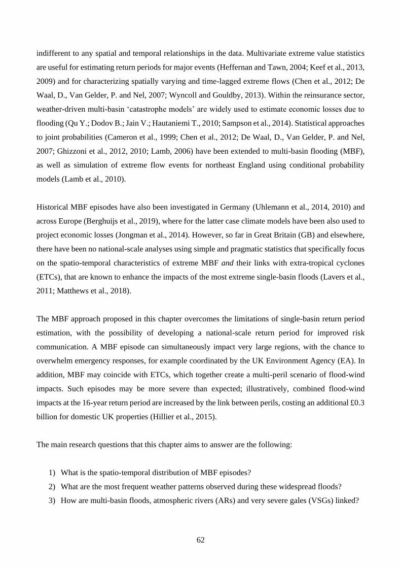
62

indifferent to any spatial and temporal relationships in the data. Multivariate extreme value statistics

are useful for estimating return periods for major events (Heffernan and Tawn, 2004; Keef et al., 2013,

2009) and for characterizing spatially varying and time-lagged extreme flows (Chen et al., 2012; De

Waal, D., Van Gelder, P. and Nel, 2007; Wyncoll and Gouldby, 2013). Within the reinsurance sector,

weather-driven multi-basin ‘catastrophe models’ are widely used to estimate economic losses due to

flooding (Qu Y.; Dodov B.; Jain V.; Hautaniemi T., 2010; Sampson et al., 2014). Statistical approaches

to joint probabilities (Cameron et al., 1999; Chen et al., 2012; De Waal, D., Van Gelder, P. and Nel,

2007; Ghizzoni et al., 2012, 2010; Lamb, 2006) have been extended to multi-basin flooding (MBF),

as well as simulation of extreme flow events for northeast England using conditional probability

models (Lamb et al., 2010).

Historical MBF episodes have also been investigated in Germany (Uhlemann et al., 2014, 2010) and

across Europe (Berghuijs et al., 2019), where for the latter case climate models have been also used to

project economic losses (Jongman et al., 2014). However, so far in Great Britain (GB) and elsewhere,

there have been no national-scale analyses using simple and pragmatic statistics that specifically focus

on the spatio-temporal characteristics of extreme MBF and their links with extra-tropical cyclones

(ETCs), that are known to enhance the impacts of the most extreme single-basin floods (Lavers et al.,

2011; Matthews et al., 2018).

The MBF approach proposed in this chapter overcomes the limitations of single-basin return period

estimation, with the possibility of developing a national-scale return period for improved risk

communication. A MBF episode can simultaneously impact very large regions, with the chance to

overwhelm emergency responses, for example coordinated by the UK Environment Agency (EA). In

addition, MBF may coincide with ETCs, which together create a multi-peril scenario of flood-wind

impacts. Such episodes may be more severe than expected; illustratively, combined flood-wind

impacts at the 16-year return period are increased by the link between perils, costing an additional £0.3

billion for domestic UK properties (Hillier et al., 2015).

The main research questions that this chapter aims to answer are the following:

1) What is the spatio-temporal distribution of MBF episodes?

2) What are the most frequent weather patterns observed during these widespread floods?

3) How are multi-basin floods, atmospheric rivers (ARs) and very severe gales (VSGs) linked?

63

This chapter therefore introduces a pragmatic approach for detecting and quantifying the

characteristics of extreme MBF episodes and their links with ETCs. It also uses new and established

metrics that could be relevant for assessing hydroclimatic impacts (Ekström et al., 2018). GB has been

used as a pilot area, but the techniques deployed are applicable wherever there are gauged river flow

data. The first research question has been answered by investigating a window of 1 to 19 days for

coincident peak flow annual maxima (AMAX) in 261 non-nested river basins during the 1975-2014

period. The reason behind choosing this time-window length is that it provides a sufficient, but not too

long, time for ETCs to completely pass through GB and for precipitation to infiltrate into the ground,

eventually enhancing runoff and flooding events. Once the MBF episodes have been identified, the

most extreme have been plotted in maps and their occurrences counted on a monthly-basis. The second

research question has been fulfilled by counting the occurrence of daily Lamb Weather Types (LWTs)

during the widespread flooding episodes. Such counts made possible the identification of the most

frequent LWTs driving MBF. Then, the third research question is addressed by simply checking if

ARs co-occurred during the most extreme MBF episodes and by correlating VSGs with MBF.

The following sections describe the data (Section 3.2), methodological approach and metrics (Section

3.3), then the six most extensive and temporally distinct MBF episodes identified, along with their

links with ETCs (Section 3.4). It is confirmed that these most extensive MBF had widespread impacts

(Environment Agency, 2003; Hulme, 1997; Kelman, 2001; Marsh and Dale, 2002; Meteorological

Office, 1992; Perry, 1980; Watkins and Whyte, 2008) and mostly occurred during winter. A

particularly powerful aspect of this approach is that it is compatible with the synoptic-scale (i.e.

~1,000km horizontal length scale) of atmospheric conditions and land-surface properties. This allows

severe MBF episodes to be evaluated alongside categories of atmospheric circulation (LWTs),

antecedent rainfall as a proxy for soil moisture (Standardized Precipitation Index, SPI), ARs, and

storminess (VSGs, frequency). Moreover, the hydrological response (joining time, Jt) for large and

small basins is examined to determine lagged responses in the system. Finally, the chapter concludes

with a discussion of the causes and implications of extreme MBF and their relationship with ETCs

(Section 3.5) and a summary of the overall research (Section 3.6).

3.2 Peak Flow and SPI Data

Highest instantaneous (15-min) peak flows (m3/s) in each water year (1st October - 30th September)

were extracted from the 1975-2014 record. These AMAX series were drawn from 261 spatially

64

representative gauged basins across GB, within a 40-year block that provides the best compromise

between spatial and temporal coverage, so that most of GB land area could have been analysed for a

sufficient longly climatic period. The network of stations is non-nested (i.e. one gauge per basin) and

covers 60.1% of GB land area (Figure 3.1). Non-nested gauging stations, as opposed to nested ones,

make it possible to consider each river basin as one individual entity, without compromising the

statistical methods by adding a bias towards the real number of basins involved in the multi-basin

floods. This is equivalent to Network A used in a previous related study (Wilby and Quinn, 2013) but

with more representative coverage across GB. The mean basin area is 482km2, ranging from 6.5km2

(Allt Leachdach) to 9,948 km2 (Thames), and average basin elevation is 149m a.s.l. Data were obtained

from the National River Flow Archive using WINFAP-FEH v4.1: http://nrfa.ceh.ac.uk/winfap-feh-

files and, for Scotland, from the Scottish Environment Protection Agency.

The SPI for timescales 24-, 18-, 12-, 6-, 3- and 1-months were obtained from the Centre for Ecology

& Hydrology (CEH) (https://catalogue.ceh.ac.uk/documents/5e1792a0-ae95-4e77-bccd-

2fb456112cc1) (Tanguy M., Kral F., Fry M., Svensson C., 2015). In this chapter all the available SPI

time-scales were used, so that sensitivity with respect to soil moisture was also quantified. The data

cover all GB within the period 1961-2012 with the territory divided into 105 Hydrometric Areas

(HAs), each with a specific SPI time series. To remain coherent with the main analysis, the SPI data

used range from 1975 to 2014, as with the chosen 40 years of hydrological records. CEH provided the

remaining two years (2013-2014) of SPI data coherent with the above dataset. To calculate a multi-

basin SPI value for an episode, the mean SPI for the HAs impacted is calculated as defined by event

set and L (see Section 3.3). Multiple AMAX on a given day are allowed because they are needed to

distinguish the HAs impacted and since each time window has been treated independently, there exist

no duplicated dates that need to be removed.

http://nrfa.ceh.ac.uk/winfap-feh-files

http://nrfa.ceh.ac.uk/winfap-feh-files

https://catalogue.ceh.ac.uk/documents/5e1792a0-ae95-4e77-bccd-2fb456112cc1

https://catalogue.ceh.ac.uk/documents/5e1792a0-ae95-4e77-bccd-2fb456112cc1

65

Figure 3.1 Network of hydrological stations and related basin areas used in the analyses. The 261 non-nested

gauges were selected from an initial network of 649 (Annex A.1.1 Figure S3.1) based on record length, and

geographic coverage. Some areas are under-represented (e.g. east England) because they are either ungauged

or do not have data for the 1975-2014 period.

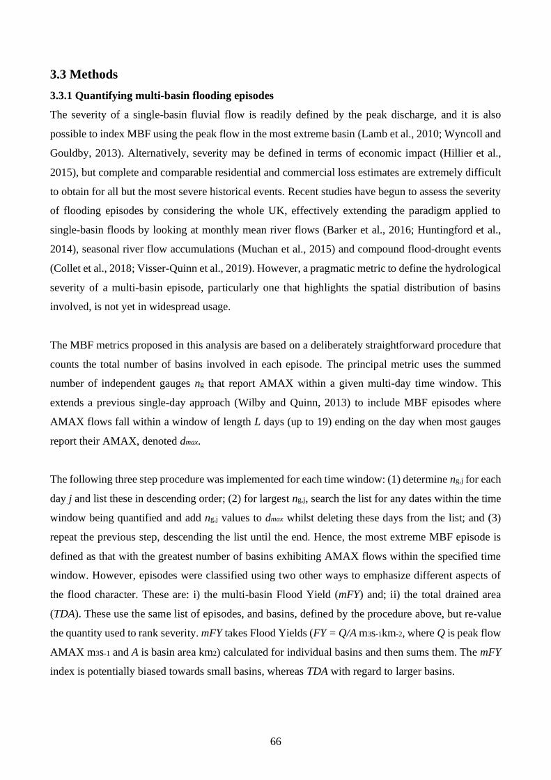
66

3.3 Methods

3.3.1 Quantifying multi-basin flooding episodes

The severity of a single-basin fluvial flow is readily defined by the peak discharge, and it is also

possible to index MBF using the peak flow in the most extreme basin (Lamb et al., 2010; Wyncoll and

Gouldby, 2013). Alternatively, severity may be defined in terms of economic impact (Hillier et al.,

2015), but complete and comparable residential and commercial loss estimates are extremely difficult

to obtain for all but the most severe historical events. Recent studies have begun to assess the severity

of flooding episodes by considering the whole UK, effectively extending the paradigm applied to

single-basin floods by looking at monthly mean river flows (Barker et al., 2016; Huntingford et al.,

2014), seasonal river flow accumulations (Muchan et al., 2015) and compound flood-drought events

(Collet et al., 2018; Visser-Quinn et al., 2019). However, a pragmatic metric to define the hydrological

severity of a multi-basin episode, particularly one that highlights the spatial distribution of basins

involved, is not yet in widespread usage.

The MBF metrics proposed in this analysis are based on a deliberately straightforward procedure that

counts the total number of basins involved in each episode. The principal metric uses the summed

number of independent gauges ng that report AMAX within a given multi-day time window. This

extends a previous single-day approach (Wilby and Quinn, 2013) to include MBF episodes where

AMAX flows fall within a window of length L days (up to 19) ending on the day when most gauges

report their AMAX, denoted dmax.

The following three step procedure was implemented for each time window: (1) determine ng,j for each

day j and list these in descending order; (2) for largest ng,j, search the list for any dates within the time

window being quantified and add ng,j values to dmax whilst deleting these days from the list; and (3)

repeat the previous step, descending the list until the end. Hence, the most extreme MBF episode is

defined as that with the greatest number of basins exhibiting AMAX flows within the specified time

window. However, episodes were classified using two other ways to emphasize different aspects of

the flood character. These are: i) the multi-basin Flood Yield (mFY) and; ii) the total drained area

(TDA). These use the same list of episodes, and basins, defined by the procedure above, but re-value

the quantity used to rank severity. mFY takes Flood Yields (FY = Q/A m3s-1km-2, where Q is peak flow

AMAX m3s-1 and A is basin area km2) calculated for individual basins and then sums them. The mFY

index is potentially biased towards small basins, whereas TDA with regard to larger basins.

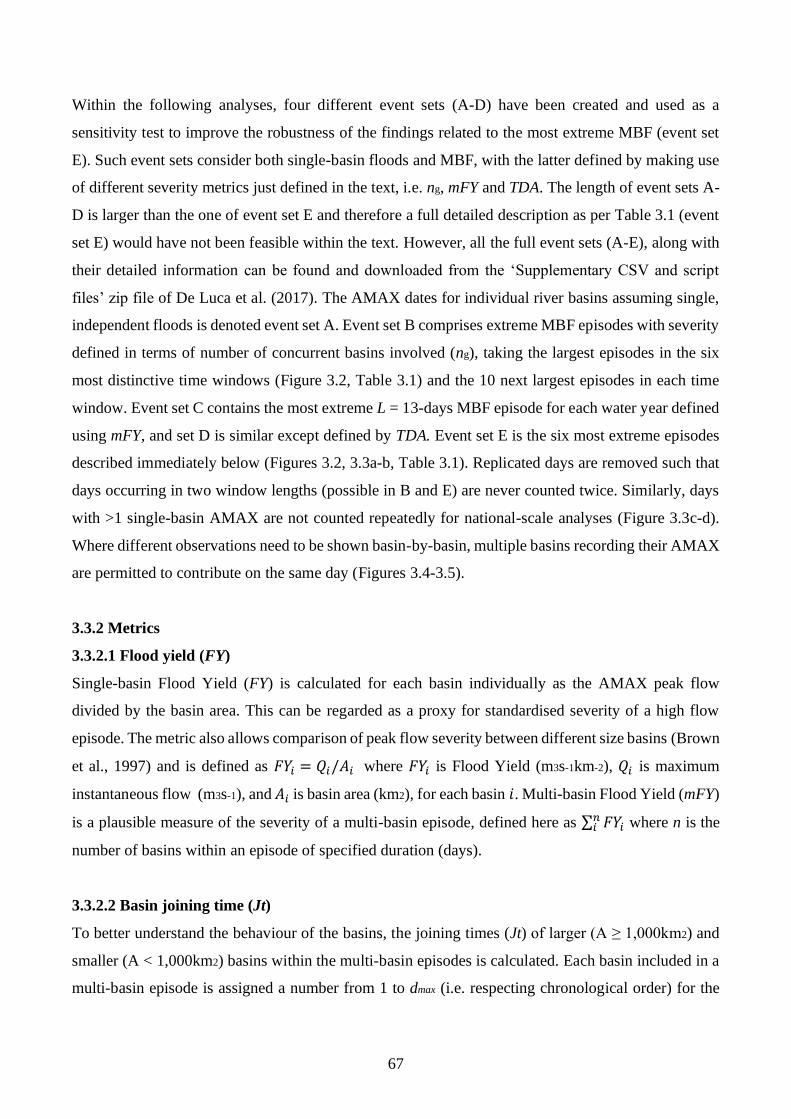
67

Within the following analyses, four different event sets (A-D) have been created and used as a

sensitivity test to improve the robustness of the findings related to the most extreme MBF (event set

E). Such event sets consider both single-basin floods and MBF, with the latter defined by making use

of different severity metrics just defined in the text, i.e. ng, mFY and TDA. The length of event sets A-

D is larger than the one of event set E and therefore a full detailed description as per Table 3.1 (event

set E) would have not been feasible within the text. However, all the full event sets (A-E), along with

their detailed information can be found and downloaded from the ‘Supplementary CSV and script

files’ zip file of De Luca et al. (2017). The AMAX dates for individual river basins assuming single,

independent floods is denoted event set A. Event set B comprises extreme MBF episodes with severity

defined in terms of number of concurrent basins involved (ng), taking the largest episodes in the six

most distinctive time windows (Figure 3.2, Table 3.1) and the 10 next largest episodes in each time

window. Event set C contains the most extreme L = 13-days MBF episode for each water year defined

using mFY, and set D is similar except defined by TDA. Event set E is the six most extreme episodes

described immediately below (Figures 3.2, 3.3a-b, Table 3.1). Replicated days are removed such that

days occurring in two window lengths (possible in B and E) are never counted twice. Similarly, days

with >1 single-basin AMAX are not counted repeatedly for national-scale analyses (Figure 3.3c-d).

Where different observations need to be shown basin-by-basin, multiple basins recording their AMAX

are permitted to contribute on the same day (Figures 3.4-3.5).

3.3.2 Metrics

3.3.2.1 Flood yield (FY)

Single-basin Flood Yield (FY) is calculated for each basin individually as the AMAX peak flow

divided by the basin area. This can be regarded as a proxy for standardised severity of a high flow

episode. The metric also allows comparison of peak flow severity between different size basins (Brown

et al., 1997) and is defined as 𝐹𝑌𝑖 = 𝑄𝑖/𝐴𝑖 where 𝐹𝑌𝑖 is Flood Yield (m3s-1km-2), 𝑄𝑖 is maximum

instantaneous flow (m3s-1), and 𝐴𝑖 is basin area (km2), for each basin 𝑖. Multi-basin Flood Yield (mFY)

is a plausible measure of the severity of a multi-basin episode, defined here as ∑ 𝐹𝑌𝑖𝑛𝑖 where n is the

number of basins within an episode of specified duration (days).

3.3.2.2 Basin joining time (Jt)

To better understand the behaviour of the basins, the joining times (Jt) of larger (A ≥ 1,000km2) and

smaller (A < 1,000km2) basins within the multi-basin episodes is calculated. Each basin included in a

multi-basin episode is assigned a number from 1 to dmax (i.e. respecting chronological order) for the

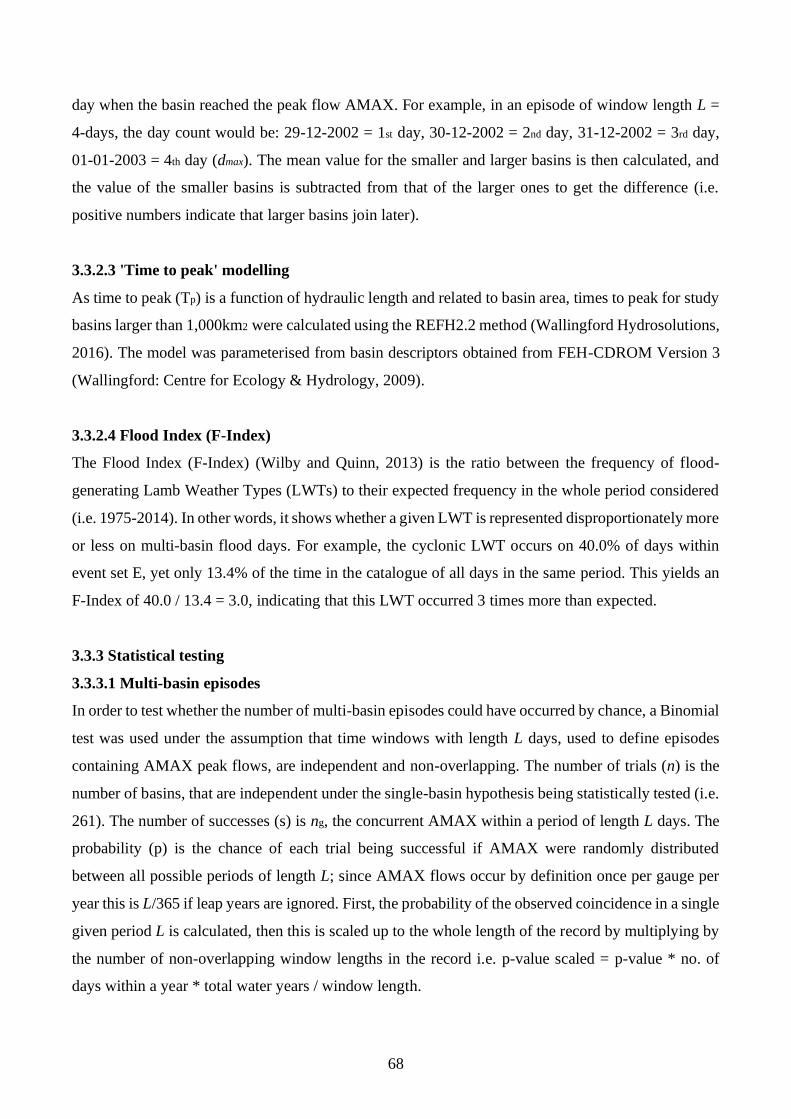
68

day when the basin reached the peak flow AMAX. For example, in an episode of window length L =

4-days, the day count would be: 29-12-2002 = 1st day, 30-12-2002 = 2nd day, 31-12-2002 = 3rd day,

01-01-2003 = 4th day (dmax). The mean value for the smaller and larger basins is then calculated, and

the value of the smaller basins is subtracted from that of the larger ones to get the difference (i.e.

positive numbers indicate that larger basins join later).

3.3.2.3 'Time to peak' modelling

As time to peak (Tp) is a function of hydraulic length and related to basin area, times to peak for study

basins larger than 1,000km2 were calculated using the REFH2.2 method (Wallingford Hydrosolutions,

2016). The model was parameterised from basin descriptors obtained from FEH-CDROM Version 3

(Wallingford: Centre for Ecology & Hydrology, 2009).

3.3.2.4 Flood Index (F-Index)

The Flood Index (F-Index) (Wilby and Quinn, 2013) is the ratio between the frequency of flood-

generating Lamb Weather Types (LWTs) to their expected frequency in the whole period considered

(i.e. 1975-2014). In other words, it shows whether a given LWT is represented disproportionately more

or less on multi-basin flood days. For example, the cyclonic LWT occurs on 40.0% of days within

event set E, yet only 13.4% of the time in the catalogue of all days in the same period. This yields an

F-Index of 40.0 / 13.4 = 3.0, indicating that this LWT occurred 3 times more than expected.

3.3.3 Statistical testing

3.3.3.1 Multi-basin episodes

In order to test whether the number of multi-basin episodes could have occurred by chance, a Binomial

test was used under the assumption that time windows with length L days, used to define episodes

containing AMAX peak flows, are independent and non-overlapping. The number of trials (n) is the

number of basins, that are independent under the single-basin hypothesis being statistically tested (i.e.

261). The number of successes (s) is ng, the concurrent AMAX within a period of length L days. The

probability (p) is the chance of each trial being successful if AMAX were randomly distributed

between all possible periods of length L; since AMAX flows occur by definition once per gauge per

year this is L/365 if leap years are ignored. First, the probability of the observed coincidence in a single

given period L is calculated, then this is scaled up to the whole length of the record by multiplying by

the number of non-overlapping window lengths in the record i.e. p-value scaled = p-value * no. of

days within a year * total water years / window length.

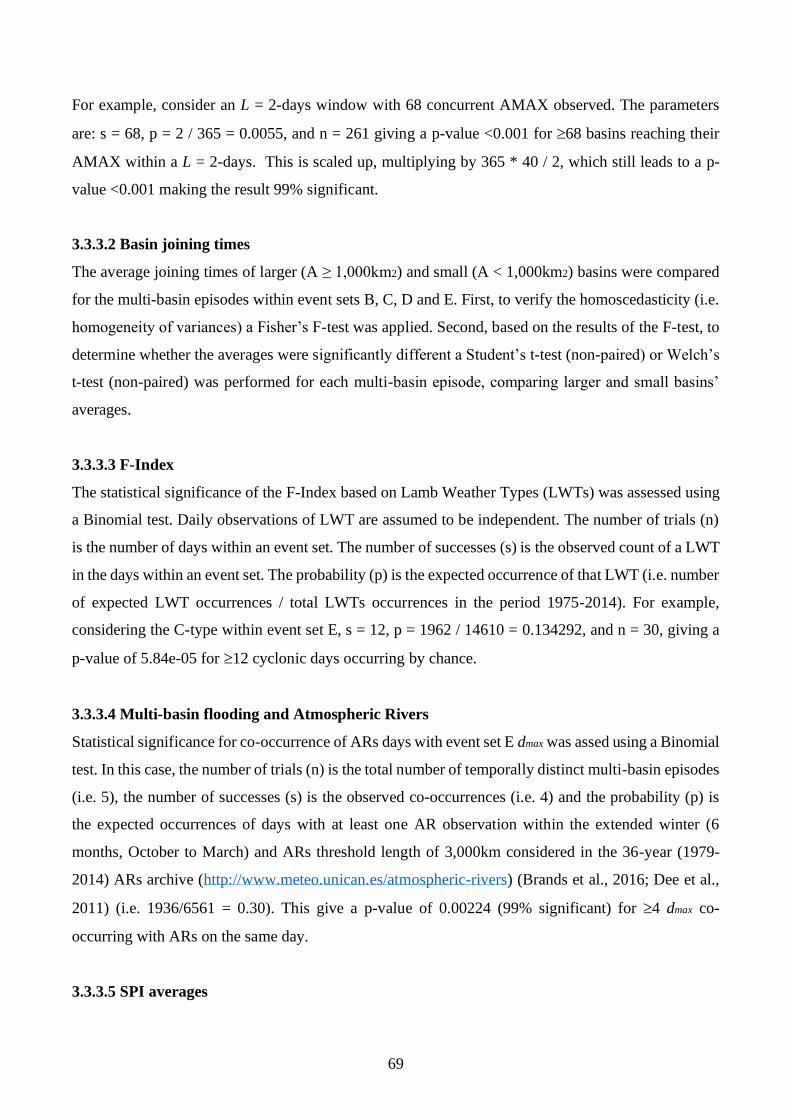
69

For example, consider an L = 2-days window with 68 concurrent AMAX observed. The parameters

are: s = 68, p = 2 / 365 = 0.0055, and n = 261 giving a p-value <0.001 for 68 basins reaching their

AMAX within a L = 2-days. This is scaled up, multiplying by 365 * 40 / 2, which still leads to a p-

value <0.001 making the result 99% significant.

3.3.3.2 Basin joining times

The average joining times of larger (A ≥ 1,000km2) and small (A < 1,000km2) basins were compared

for the multi-basin episodes within event sets B, C, D and E. First, to verify the homoscedasticity (i.e.

homogeneity of variances) a Fisher’s F-test was applied. Second, based on the results of the F-test, to

determine whether the averages were significantly different a Student’s t-test (non-paired) or Welch’s

t-test (non-paired) was performed for each multi-basin episode, comparing larger and small basins’

averages.

3.3.3.3 F-Index

The statistical significance of the F-Index based on Lamb Weather Types (LWTs) was assessed using

a Binomial test. Daily observations of LWT are assumed to be independent. The number of trials (n)

is the number of days within an event set. The number of successes (s) is the observed count of a LWT

in the days within an event set. The probability (p) is the expected occurrence of that LWT (i.e. number

of expected LWT occurrences / total LWTs occurrences in the period 1975-2014). For example,

considering the C-type within event set E, s = 12, p = 1962 / 14610 = 0.134292, and n = 30, giving a

p-value of 5.84e-05 for 12 cyclonic days occurring by chance.

3.3.3.4 Multi-basin flooding and Atmospheric Rivers

Statistical significance for co-occurrence of ARs days with event set E dmax was assed using a Binomial

test. In this case, the number of trials (n) is the total number of temporally distinct multi-basin episodes

(i.e. 5), the number of successes (s) is the observed co-occurrences (i.e. 4) and the probability (p) is

the expected occurrences of days with at least one AR observation within the extended winter (6

months, October to March) and ARs threshold length of 3,000km considered in the 36-year (1979-

2014) ARs archive (http://www.meteo.unican.es/atmospheric-rivers) (Brands et al., 2016; Dee et al.,

2011) (i.e. 1936/6561 = 0.30). This give a p-value of 0.00224 (99% significant) for 4 dmax co-

occurring with ARs on the same day.

3.3.3.5 SPI averages

http://www.meteo.unican.es/atmospheric-rivers

70

In order to check the statistical significance of the SPI observations within event set B, in a similar

way of Section 3.3.3.2 a Fisher’s F-test and t-test (non-paired) were used to compare the mean SPI on

the days within the episodes to the overall record (i.e. 40-year, 1975-2014). These tests are repeated

for each time window and SPI time range (i.e. 24-, 18-, 12-, 6-, 3-, and 1-month) and after Fisher’s F-

test, if the variances are equal the Student’s t-test was applied, otherwise Welch’s t-test was used.

3.3.3.6 Peak flows and very severe gales

The interaction between extreme mFY episodes and VSG was assessed as follows. Years with both the

most severe flows (30%) and wind (50%) were selected. Given a record of 40 years, the expected

number of years where both are severe is simply E = 0.3*0.5*40 = 6.6, but actually 10 were observed.

Following the methodology of an earlier study (Hillier et al., 2015), a Monte Carlo simulation (with

10,000 iterations) was run to determine how often 10 co-occurrences occur by chance. In this case,

the relative p-value is set at 0.021. In the simulation 12 (i.e. 40*0.3) random years (1975-2014) were

assigned to ‘flood’ in each 40-year realization, as were 20 (i.e. 40*0.5) assigned to be severe for wind.

The number of co-occurrences was counted for each of the 10,000 realizations to determine the

probability.

The timing of episodes, within the 10 years, where both severe multi-basin flows and winds occurred

together is investigated using the Binomial test. The dates, within event set C, where the largest number

of concurrent basins were detected (i.e. dmax) were compared to dates where VSG occurred. Therefore,

in a similar way of Section 3.3.3.1 and Section 3.3.3.3, the tasks to address were to test: i) if the

occurrence of 5 out of 10 high flows on the same day of a VSG is coincidental (i.e. what is the chance

of 5 occurrences?), and ii) if the occurrence of dmax during a period including the day of VSG and up

to 13-days afterwards is coincidental (i.e. what is the chance of 9 occurrences?). For the first task,

the number of trials (n) is the number of years (i.e. 10), the number of successes (s) correspond to the

combined occurrences (i.e. 5) and the probability (p) is the chance of each trial being successful during

the whole 10 years, i.e. 49 / 3650 = 0.0134, where 49 are the days with a VSG and 3650 the total days

within a 10-year period. Whereas for the second task (n) is still the number of years (i.e. 10), the

number of successes (s) is now 9 and the probability (p) is equal to 487 / 3650 = 0.133.

3.4 Results

3.4.1 Characterizing severe MBF episodes

71

The most extreme MBF episodes defined using ng, obtained from 19 time window lengths, comprise

five temporally distinct episodes (event set E, Table 3.1). These are: dmax = 27/12/1979 (66 basins

involved, 18.6% of study area, window length L = 1-day); 30/10/2000 (68, 14.1%, L = 2-days);

01/01/2003 (75, 24.9%, L = 4-days); 02/12/1992 (96, 22%, L = 8-days); and 01/02/1995 (108, 46.5%,

L = 16-days). If different time windows return the same date, the window with the largest number of

concurrent AMAX is given. However, the L = 6-days episode (30/10/2000, Figure 3.2d, Table 3.1) is

included because the number of basins involved (86) and drained fraction of the study area (19.8%)

are both much larger than the L = 2-days episode. Figure 3.2 shows the regional distribution and basin-

by-basin FY severity of these six episodes.

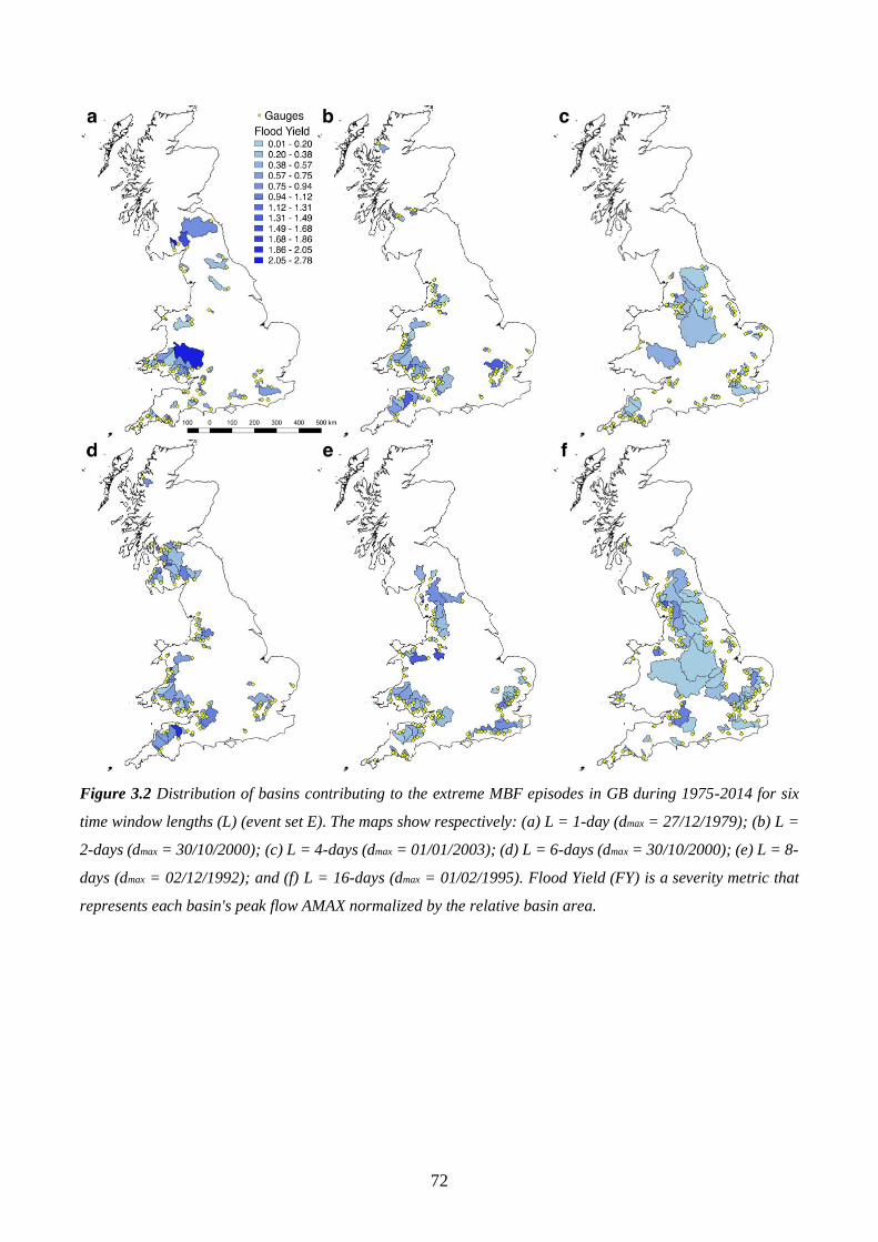
72

Figure 3.2 Distribution of basins contributing to the extreme MBF episodes in GB during 1975-2014 for six

time window lengths (L) (event set E). The maps show respectively: (a) L = 1-day (dmax = 27/12/1979); (b) L =

2-days (dmax = 30/10/2000); (c) L = 4-days (dmax = 01/01/2003); (d) L = 6-days (dmax = 30/10/2000); (e) L = 8-

days (dmax = 02/12/1992); and (f) L = 16-days (dmax = 01/02/1995). Flood Yield (FY) is a severity metric that

represents each basin's peak flow AMAX normalized by the relative basin area.

73

The ng metric ranges from 66 (L = 1-day) to 108 (L = 16-days) river basins, plateauing at L 13-days

(Figure 3.3a). For all time windows, the number of co-occurrences is notably larger than expected by

chance (p-value <0.01, Binomial test). The TDA ranges from 17,787km2 (L = 2-days) to 58,491km2 (L

= 16-days), again plateauing at L 13-days (Figure 3.3b). These areas correspond to 14.1% and 46.5%

of the area of the 261 gauged basins respectively, or 8.5% and 27.9% of the total land area of GB

(Figure 3.3b, Table 3.1). L = 13-days defines event sets C and D as this window length captures the

largest episodes whilst retaining the maximum temporal resolution.

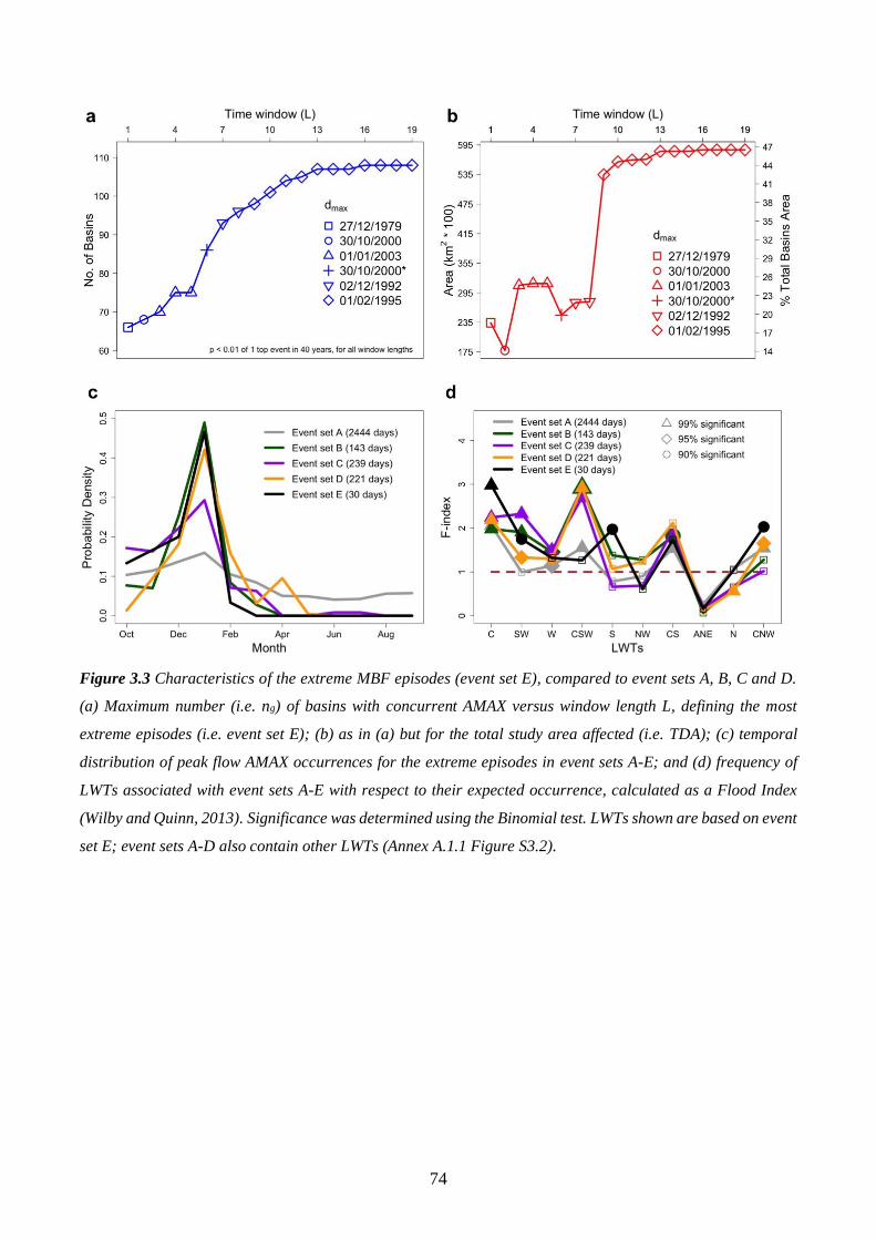
74

Figure 3.3 Characteristics of the extreme MBF episodes (event set E), compared to event sets A, B, C and D.

(a) Maximum number (i.e. ng) of basins with concurrent AMAX versus window length L, defining the most

extreme episodes (i.e. event set E); (b) as in (a) but for the total study area affected (i.e. TDA); (c) temporal

distribution of peak flow AMAX occurrences for the extreme episodes in event sets A-E; and (d) frequency of

LWTs associated with event sets A-E with respect to their expected occurrence, calculated as a Flood Index

(Wilby and Quinn, 2013). Significance was determined using the Binomial test. LWTs shown are based on event

set E; event sets A-D also contain other LWTs (Annex A.1.1 Figure S3.2).

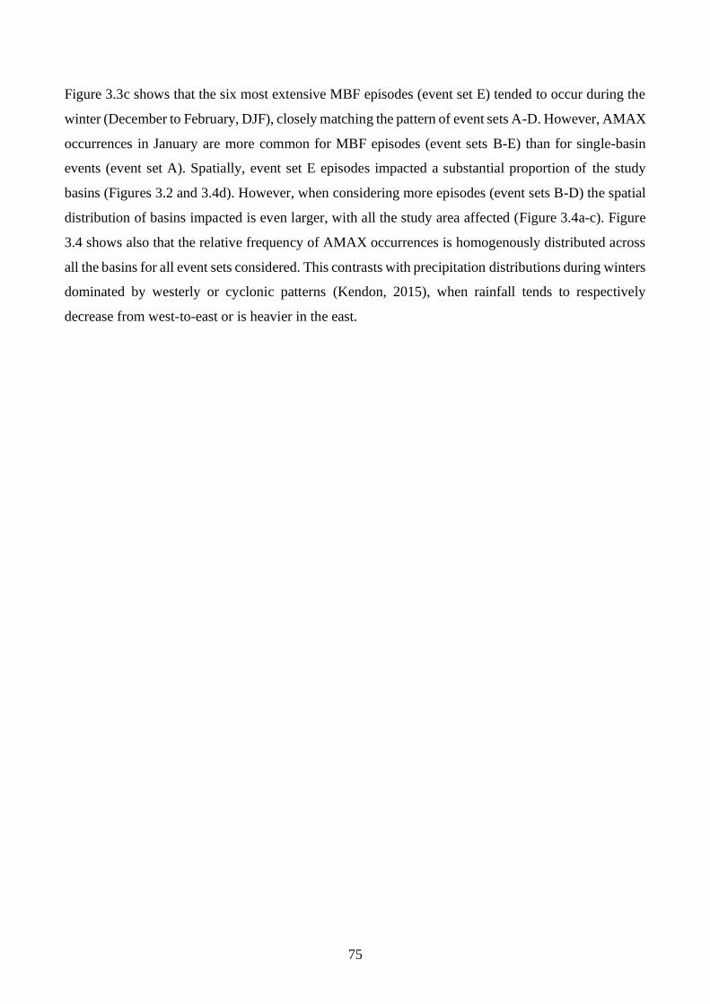
75

Figure 3.3c shows that the six most extensive MBF episodes (event set E) tended to occur during the

winter (December to February, DJF), closely matching the pattern of event sets A-D. However, AMAX

occurrences in January are more common for MBF episodes (event sets B-E) than for single-basin

events (event set A). Spatially, event set E episodes impacted a substantial proportion of the study

basins (Figures 3.2 and 3.4d). However, when considering more episodes (event sets B-D) the spatial

distribution of basins impacted is even larger, with all the study area affected (Figure 3.4a-c). Figure

3.4 shows also that the relative frequency of AMAX occurrences is homogenously distributed across

all the basins for all event sets considered. This contrasts with precipitation distributions during winters

dominated by westerly or cyclonic patterns (Kendon, 2015), when rainfall tends to respectively

decrease from west-to-east or is heavier in the east.

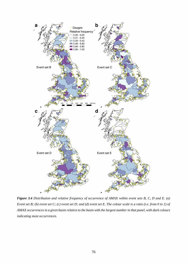
76

Figure 3.4 Distribution and relative frequency of occurrence of AMAX within event sets B, C, D and E. (a)

Event set B; (b) event set C; (c) event set D; and (d) event set E. The colour scale is a ratio (i.e. from 0 to 1) of

AMAX occurrences in a given basin relative to the basin with the largest number in that panel, with dark colours

indicating most occurrences.

77

The average Jt for larger (A 1,000km2) and smaller (A <1,000km2) basins within MBF episodes was

compared. Considering time-windows (L) separately for event set E, only when L = 2- or 16-days do

larger basins join significantly later (t-test non-paired), and the delays were modest, just 0.1 and 1.8

days respectively (Table 3.1). Event sets B-D replicate this, showing occasional significance but

joining times < 48h. A Tp response analysis (Wallingford: Centre for Ecology & Hydrology, 2009;

Wallingford Hydrosolutions, 2016) for larger basins further indicates Tp <40h, again less than the ~13-

day time-span that appears to define extreme MBF episodes.

For the six main episodes (event set E), maximum FY tend to be greater for short time windows. For

example, it is 2.6 m3s-1km-2 at L = 1-day, and 2.0 m3s-1km-2 at L = 2-days compared with 1.9 and 1.5

m3s-1km-2 for L = 8- and 16-days respectively. All these basins have TDA < 71km2 which is below the

network mean (482km2).

3.4.2 Relationship to inundation episodes

Severity measured by ng is a proxy for overbank flow and fluvial flood extent. Only a fraction of the

basin areas will be inundated. However, the six extreme MBF episodes (event set E, Figure 3.2) all

resulted in widespread flooding demonstrating the relevance of the AMAX multi-basin severity metric

as a diagnostic:

• The December 1979 episode (Figure 3.2a) was the most severe in South Wales since 1960 and

in some areas the worst in a century, causing extensive floods that killed four people,

necessitated the evacuation of hundreds and caused millions of pounds of damage (Perry,

1980).

• The Autumn 2000 episodes (Figure 3.2b and d) were described as the most devastating in

England since 1947, and associated with the wettest 12-month period since 1776 (Kelman,

2001; Marsh and Dale, 2002).

• The January 2003 episode (Figure 3.2c) was reported by the EA in FloodLink (Environment

Agency, 2003) with most severe floods in the East Midlands, where the Trent basin had 118

flood warnings and 14 flood watches issued between 29/12/2002 and 03/01/2003.

• The November/December 1992 episode (Figure 3.2e) was reported by the UK Met Office

(Meteorological Office, 1992) after floods impacted southern England during the night of

25th/26th November. However, the worst phase occurred on the 29th, when flooding in Wales

devastated homes and caused widespread road and railway disruptions.

78

• The February 1995 episode (Figure 3.2f) caused severe floods on at least 7 rivers, following

heavy frontal precipitation in January 1995 which was 79% above the 1961-1990 average

(Hulme, 1997; Watkins and Whyte, 2008).

3.4.3 Relationship to atmospheric patterns

Daily UK synoptic-scale atmospheric patterns can be characterized by LWTs (Jones et al., 2013;

Lamb, 1972). The frequency of LWTs for days during extreme single- and multi-basin peak flow

episodes was compared with the entire 40-year catalogue of LWTs (Figure 3.3d). In this comparison,

a F-Index (Wilby and Quinn, 2013) is defined as the ratio of observed to expected frequency of LWTs.

This was undertaken for event sets: A (2444 days), B (143 days), C (239 days), D (221 days) and E

(30 days), excluding replicate dates. Statistical significance of the F-Index was calculated using a

Binomial test.

Overall, the cyclonic (C-type) LWT is most definitively associated with the peak flows with a 99%

statistically significant F-Index 1.98 for all event sets considered, ~3 times more than expected for

event set E. The south-westerly (SW), westerly (W), and cyclonic SW (CSW) types are also associated

with AMAX events (p-value <0.01, 0.05 and 0.1, Binomial test), and therefore more likely linked with

widespread flooding. Southerly (S) types are significantly represented in event sets E, but not in event

sets A-D (Figure 3.3d). Therefore, a pattern of C- and W-types contributing to widespread peak flows

is depicted and the multi-basin event sets B-E show very similar F-Index results when compared to

single-basin AMAX (event set A, Annex A.1.1 Figure S3.3).

It is also of interest if these circulation systems are particularly ‘wet’. ARs are corridors of intense

horizontal water vapour transport within the warm conveyor belt of ETCs (Lavers et al., 2013, 2011).

dmax dates of the event set E episodes are compared with an ARs archive (Brands et al., 2016; Dee et

al., 2011). Four out of the five temporally distinct MBF episodes occurred on the same day as an AR,

which on average happen on only 30% of extended (Oct-Mar) winter days (p-value <0.01, Binomial

test).

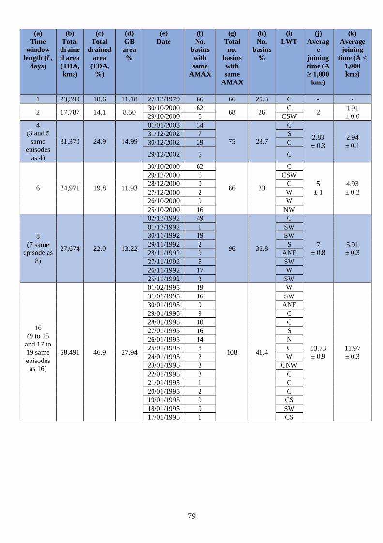
79

(a)

Time

window

length (L,

days)

(b)

Total

draine

d area

(TDA,

km2)

(c)

Total

drained

area

(TDA,

%)

(d)

GB

area

%

(e)

Date

(f)

No.

basins

with

same

AMAX

(g)

Total

no.

basins

with

same

AMAX

(h)

No.

basins

%

(i)

LWT

(j)

Averag

e

joining

time (A

≥ 1,000

km2)

(k)

Average

joining

time (A <

1,000

km2)

1 23,399 18.6 11.18 27/12/1979 66 66 25.3 C - -

2 17,787 14.1 8.50 30/10/2000 62

68 26 C

2 1.91

± 0.0 29/10/2000 6 CSW

4

(3 and 5

same

episodes

as 4)

31,370 24.9 14.99

01/01/2003 34

75 28.7

C

2.83

± 0.3

2.94

± 0.1

31/12/2002 7 S

30/12/2002 29 C

29/12/2002 5 C

6 24,971 19.8 11.93

30/10/2000 62

86 33

C

5

± 1

4.93

± 0.2

29/12/2000 6 CSW

28/12/2000 0 C

27/12/2000 2 W

26/10/2000 0 W

25/10/2000 16 NW

8

(7 same

episode as

8)

27,674 22.0 13.22

02/12/1992 49

96 36.8

C

7

± 0.8

5.91

± 0.3

01/12/1992 1 SW

30/11/1992 19 SW

29/11/1992 2 S

28/11/1992 0 ANE

27/11/1992 5 SW

26/11/1992 17 W

25/11/1992 3 SW

16

(9 to 15

and 17 to

19 same

episodes

as 16)

58,491 46.9 27.94

01/02/1995 19

108 41.4

W

13.73

± 0.9

11.97

± 0.3

31/01/1995 16 SW

30/01/1995 9 ANE

29/01/1995 9 C

28/01/1995 10 C

27/01/1995 16 S

26/01/1995 14 N

25/01/1995 3 C

24/01/1995 2 W

23/01/1995 3 CNW

22/01/1995 3 C

21/01/1995 1 C

20/01/1995 2 C

19/01/1995 0 CS

18/01/1995 0 SW

17/01/1995 1 CS

80

Table 3.1 Extreme MBF episodes in GB during 1975-2014 (event set E). Observations are derived from 19 time

windows up to 18 days prior dmax; see main text for details. (a) Window length (L) in days; (b) Total drained

area (TDA, km2) involved in each episode (i.e. sum of the area of all involved basins); (c) Percentage of TDA

of the 261 basins affected by each episode; (d) Percentage of GB land area affected by each episode; (e) Dates

of episodes, where the top row represents dmax; (f) Number of basins with peak flow AMAX registered on the

same day; (g) Total number of basins with peak flow AMAX per episode; (h) Percentage of total number of

basins (out of 261) with concurrent AMAX per episode; (i) Daily LWT; (j) Average joining time, within an

episode, for larger basins (A 1,000km2); (k) Average joining time for small basins (A <1,000km2). In (j) and

(k) uncertainties are 1 standard error of the mean.

3.4.4 Relationship with antecedent soil moisture conditions

High soil moisture content increases the likelihood of flooding. The SPI (McKee T.B., Doesken N.J.,

1995; McKee et al., 1993) is widely used as a proxy for this physical property and 3-24 month SPI

values are distinctively high for historical episodes (Du et al., 2013; Seiler et al., 2002; Wang et al.,

2015). Whilst the sample of episodes in event set E is too small to show a pattern, SPI aggregated

across impacted basins (Tanguy M., Kral F., Fry M., Svensson C., 2015) is significantly (p-value

<0.05, t-test non-paired) higher than average across all L for event set B (p-value <<0.01), increasing

with L (Figure 3.5). Event set C, by incorporating a forced regularized annual sampling, demonstrates

that flood magnitude is greater in ‘wet’ spells (SPI >0.5) than ‘dry’ periods (SPI <-0.5) with mean

mFY = 26.93.4 (1) and 17.11.3 (1) respectively for SPI-12. Indeed, for this comparison, all except

SPI-1 are significant (p-value <0.05, t-test, 2-tailed). Event set D (based on TDA) shows no signal for

this well-established flood-SPI connection, suggesting that the metric based on mFY (event set C)

might better reflect physical processes.

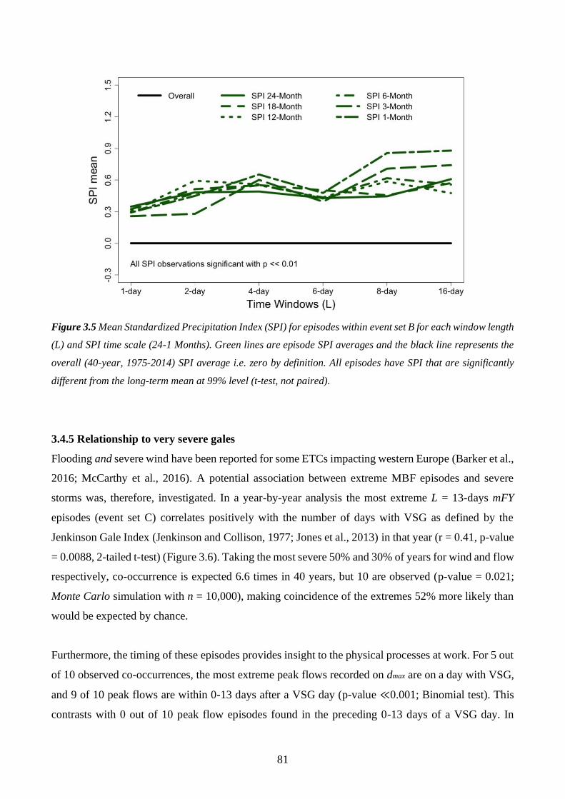
81

Figure 3.5 Mean Standardized Precipitation Index (SPI) for episodes within event set B for each window length

(L) and SPI time scale (24-1 Months). Green lines are episode SPI averages and the black line represents the

overall (40-year, 1975-2014) SPI average i.e. zero by definition. All episodes have SPI that are significantly

different from the long-term mean at 99% level (t-test, not paired).

3.4.5 Relationship to very severe gales

Flooding and severe wind have been reported for some ETCs impacting western Europe (Barker et al.,

2016; McCarthy et al., 2016). A potential association between extreme MBF episodes and severe

storms was, therefore, investigated. In a year-by-year analysis the most extreme L = 13-days mFY

episodes (event set C) correlates positively with the number of days with VSG as defined by the

Jenkinson Gale Index (Jenkinson and Collison, 1977; Jones et al., 2013) in that year (r = 0.41, p-value

= 0.0088, 2-tailed t-test) (Figure 3.6). Taking the most severe 50% and 30% of years for wind and flow

respectively, co-occurrence is expected 6.6 times in 40 years, but 10 are observed (p-value = 0.021;

Monte Carlo simulation with n = 10,000), making coincidence of the extremes 52% more likely than

would be expected by chance.

Furthermore, the timing of these episodes provides insight to the physical processes at work. For 5 out

of 10 observed co-occurrences, the most extreme peak flows recorded on dmax are on a day with VSG,

and 9 of 10 peak flows are within 0-13 days after a VSG day (p-value ≪0.001; Binomial test). This

contrasts with 0 out of 10 peak flow episodes found in the preceding 0-13 days of a VSG day. In

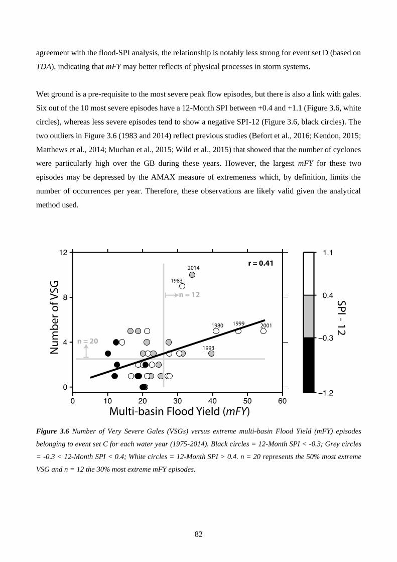
82

agreement with the flood-SPI analysis, the relationship is notably less strong for event set D (based on

TDA), indicating that mFY may better reflects of physical processes in storm systems.

Wet ground is a pre-requisite to the most severe peak flow episodes, but there is also a link with gales.

Six out of the 10 most severe episodes have a 12-Month SPI between +0.4 and +1.1 (Figure 3.6, white

circles), whereas less severe episodes tend to show a negative SPI-12 (Figure 3.6, black circles). The

two outliers in Figure 3.6 (1983 and 2014) reflect previous studies (Befort et al., 2016; Kendon, 2015;

Matthews et al., 2014; Muchan et al., 2015; Wild et al., 2015) that showed that the number of cyclones

were particularly high over the GB during these years. However, the largest mFY for these two

episodes may be depressed by the AMAX measure of extremeness which, by definition, limits the

number of occurrences per year. Therefore, these observations are likely valid given the analytical

method used.

Figure 3.6 Number of Very Severe Gales (VSGs) versus extreme multi-basin Flood Yield (mFY) episodes

belonging to event set C for each water year (1975-2014). Black circles = 12-Month SPI < -0.3; Grey circles

= -0.3 < 12-Month SPI < 0.4; White circles = 12-Month SPI > 0.4. n = 20 represents the 50% most extreme

VSG and n = 12 the 30% most extreme mFY episodes.

83

3.5 Discussion

3.5.1 A new multi-basin approach

Various diagnostics for the evaluation of MBF episodes were presented here. The first metric detects

key ‘episodes’ by summing the concurrent number of basins (i.e. ng) attaining their AMAX within a

given time window, then ranking the episodes based on ng. Once basins contributing to each episode

are identified other metrics can characterize different aspects of the episodes. When episodes are

identified in terms of ng, this gives perhaps undue weight to small basins, but TDA emphasizes larger

rivers. The mFY can either weight small basins, when calculated as here or large ones if area and flow

were each summed before dividing them. All are practical options, but awareness of any biases and

use of multiple metrics is recommended to ensure robust insights.

There are various advantages with this approach to MBF analysis. First, it enables the identification

of extreme peak-flow episodes that are driven by persistent rain-bearing weather systems by

accounting for variations in time-lags before peak flow that depend on precipitation properties, basin

area and geology. Second, it provides a national-scale flood measure allowing more meaningful

comparison with synoptic-scale weather patterns than at the scale of individual basins, no matter how

large (Hillier et al., 2015). Third, whichever metric is selected a return period that is applicable across

a whole country can be estimated.

A single, national rather than basin-scale, return period has a potentially important role in risk

communication. Such metrics could address the question often posed to flood managers: “Why is there

a 1 in 100-year flood event every year?” This impression arises because return period estimates are

traditionally based on flows at a single gauge. The MBF metrics proposed in this chapter would yield

the 1-in-100 year episode based on a return period estimate that integrates information across all basins

in a network.

3.5.2 Widespread concurrent impacts

Answers to the first and second research questions posed in Section 3.1 are here presented and

discussed. Results show that extreme MBF episodes can affect large areas (Figure 3.2), with likely

commensurate damages (Environment Agency, 2003; Hulme, 1997; Kelman, 2001; Marsh and Dale,

2002; Meteorological Office, 1992; Perry, 1980; Watkins and Whyte, 2008). For instance, the L = 16-

days episode captures ~46% of the study area (or ~27% of GB) with 108 basins concurrently reaching

their AMAX (Figures 3.2f, 3.3a-b, Table 3.1). Aspects of the physical processes driving these

84

widespread episodes appear similar to those deduced from single-basin studies (Barker et al., 2016;

Blöschl et al., 2015; Huntingford et al., 2014; Kendon, 2015; Merz, R. Blöschl, 2003; Merz et al.,

2014; Muchan et al., 2015; Nied et al., 2016; Schaller et al., 2016). First, W- and C-type LWTs

associated with MBF (Figure 3.3d, Table 3.1) have been linked to frequent floods (Pattison and Lane,

2012; Wilby and Quinn, 2013), the wettest winters in England and Wales (Kendon, 2015; Kendon and

McCarthy, 2015), and >80% of extreme flows on the River Eden (UK) (Pattison and Lane, 2012). The

W-type, in particular, represents one of the main drivers of high rainfall and flows in the UK

(Hannaford and Marsh, 2008; Pattison and Lane, 2012) as well as flooding throughout central Europe

(Pattison and Lane, 2012). Second, maximum FY occur in smaller basins (<71km2). This is consistent

with higher expected flood severity in smaller basins which respond more rapidly to any given storm.

Third, MBF is larger (by mFY) in wet years (SPI >0.5), and in longer time windows when SPI is

higher.

The observation that single-basin flooding in GB occurs mostly during winter also applies to MBF

episodes (Figure 3.3c). This is due to frequent storms and their associated precipitation (Matthews et

al., 2018, 2016b), combined with lower evapotranspiration, and wetter antecedent soil conditions

(Figure 3.5) that ultimately combine to generate higher flows (Blöschl et al., 2015; Huntingford et al.,

2014). However, the largest MBF episodes are most common in January (Figure 3.3c), when the most

favourable conditions (C, SW, W and CSW circulation types) are more likely.

A key feature that distinguishes large MBF episodes from their single-basin counterparts is their

duration (i.e. 13-days, Figure 3.3a-b). This is greater than currently accounted for in other studies

(Cameron et al., 1999), and indicates that a notable 'memory' in the physical system is required. With

a Tp <40h (Wallingford: Centre for Ecology & Hydrology, 2009; Wallingford Hydrosolutions, 2016),

this cannot be within the channelized flow paths, a view supported empirically by larger basins joining

episodes at essentially the same time as smaller ones (Table 3.1 and Annex A.1.1 Figure S3.4). This

observation also rules out reservoirs delaying flow outside of the channels, and is reconciled by the

fact that concentration time increases with basin area (Grimaldi et al., 2016). Thus, the memory should

exist in either antecedent soil or groundwater levels (Du et al., 2013; Seiler et al., 2002; Wang et al.,

2015) (Figures 3.5-3.6), or in persistent atmospheric patterns during notably wet years (Barker et al.,

2016; Huntingford et al., 2014; Kendon, 2015; Matthews et al., 2018; McCarthy et al., 2016; Muchan

et al., 2015; Wild et al., 2015). These elements of memory likely exist for larger European rivers (e.g.

85

Rhine), although they are less easily decoupled because time-scales attributable to the processes

overlap more.

3.5.3 Compounding flood and wind impacts

The third research question highlighted in Section 3.1 is also answered and discussed in this

subparagraph. ETCs were identified as a driver of MBF episodes (via cyclonic LWT and ARs). When

considering these high flows in terms of extreme mFY for each water year within L = 13-days (event

set C), a relationship with damaging winds predominantly caused by ETCs is also demonstrated. A

significantly positive correlation exists between VSG and MBF episodes, with co-occurrence of

extremes 52% more likely than by chance and high flows occurring within 0-13 days after a VSG day.

Building on case studies of notable years (Huntingford et al., 2014; Kendon, 2015; Matthews et al.,

2014; Muchan et al., 2015; Schaller et al., 2016; Wild et al., 2015) and the Trent basin in central

England (Hillier et al., 2015), this is the first systematic, national-scale evidence that the severest

aspects of wet and windy winters tend to co-occur. Often these phenomena are viewed separately:

severe ETCs bring extreme winds (Pinto et al., 2009) whilst slower moving, less windy ETCs bring

large accumulated rainfall totals and extensive flooding in GB (Burt et al., 2015; Matthews et al.,

2016b; Wilby and Quinn, 2013). Thus, the evidence of coincident widespread flood and wind on the

same day in 5 out of 10 years and within 13 days in another 4 of those years contradicts a prevailing

view that Storm Desmond was exceptional in bringing both very severe wind and widespread flooding

(Barker et al., 2016; Matthews et al., 2018; McCarthy et al., 2016). These findings also highlight the

importance of considering longer time-lags when assessing dependencies between weather-driven

hazards where both may not occur in the same defined extreme episode. As far the author is aware,

this is the first statistical evidence of a time-lagged link between widespread flooding and severe wind

for any nation. This methodology also enables potential detection of such inter-dependencies

elsewhere. Moreover, as for single-basin floods (Lavers et al., 2011), extreme MBF episodes co-

occurred with ARs.

One implication of coincident floods and severe winds is that worst-case years are likely more severe

than previously thought. With the association apparently strongest for the most extreme episodes, the

effect of this co-occurrence on annualized aggregate insurance losses could exceed the £0.3 billion

reported for UK domestic properties for a 16-year return period event (Hillier et al., 2015). Moreover,

GB is located beneath the North Atlantic storm track and is, therefore, affected by the passage of ETCs

(Matthews et al., 2016b) which bring extreme winds (Matthews et al., 2018; Pinto et al., 2009) that

can subsequently affect central Europe (Donat M. G., Leckebusch G. C., Pinto J. G., 2010). Since

86

ETCs can continue to strengthen after landfall, this effect may extend to a much larger physical and

financial scale than the GB alone. Furthermore, there is a likely three-way association between

widespread flooding, severe wind and storm surges that warrants investigation.

3.5.4 Operational implications

The EA is responsible for contingency planning, forecasting and managing the consequences of

widespread flood episodes. Regional ‘footprints’ of past severe episodes (Figure 3.2) reveal the extent

to which authorities in neighbouring areas could be impacted simultaneously. This is relevant when

coordinating and sharing equipment and personnel during such episodes. For instance, the Midlands

region of the EA lies in a pivotal location since it may be called upon to provide resources to affected

areas to the North and South. During the severe flooding in December 2015, personnel and equipment

were drawn from regions hundreds of kilometres away from the epicentre of Northwest England and

Southern Scotland. This might not be feasible in the event of a MBF episode on the scale of

January/February 1995 (Figure 3.2f). However, knowledge of the likelihood and pattern of MBF

provides a basis for role-play exercises as part of the contingency planning for such episodes.

Both the UK National Flood Resilience Review (HM Government, 2016) and CCRA (ASC, 2016)

recognise interdependencies between critical networks (e.g. electricity, water and transport) and the

need to manage indirect flood impacts on the economy. However, their emphasis remains on

integrated, yet single-basin solutions involving ‘natural’ flood management, improved property- and

asset-level resilience, and planning controls. Widespread flooding in Australia in 2011, and multiple

events in Central Europe since 2002, show the need for a higher-level strategy for managing extensive,

transboundary flooding (Wilby and Keenan, 2012). Moreover, the likelihood of MBF episodes could

increase with ETCs intensity and ARs frequency and magnitude expected to rise under anthropogenic

climate change (Donat M. G., Leckebusch G. C., Pinto J. G., 2010; Donat et al., 2010; Lavers et al.,

2013; Matthews et al., 2018, 2016b; Ulbrich et al., 2009; Zappa et al., 2013).

3.5.5 Storms since 2014

The analysis conducted in this chapter ends in water-year 2014 and since then, the UK was affected

by the passage of other impactful ETCs, causing socio-economic disruption. During storm season

2015-2016, when the Met Office and Met Éireann officially started to provide a name to storms, there

were 11 ETCs impacting the UK and/or Ireland (Met Office). The most noticeable was Storm

Desmond (Burt et al., 2016; Matthews et al., 2018; Wilby and Barker, 2016), that caused record-

breaking flooding over Cumbria and Lancashire, with 5,200 homes flooded and more than 50,000

87

without power in north-eastern England (Met Office). During storm season 2016-2017 only five ETCs

were named (Met Office). The most impactful was Storm Doris, which was characterised by strong

wind gusts up to 94 mph in north Wales and heavy snowfall in Scotland. Lastly, in 2017-2018 season

a total of 8 storms impacted the UK and/or Ireland (Met Office). In this 10-month period the most

significant storms were Eleanor and Hector. The former impacted the UK during January 2018 with

wind gusts up to 100 mph in Cumbria, causing widespread transport disruption and power cuts, along

with storm surges. On the other hand, the latter occurred in June 2018 and was characterised by strong

winds and heavy rainfall in the UK and Ireland, eventually leading to road and rail disruption and

fallen trees (Met Office).

3.6 Summary

The focus of the above research is on the smallest geographical domain of the thesis, which is Great

Britain (GB), yet contributes to knowledge about the interactions between extreme multi-basin floods

and extra-tropical cyclones (ETCs) (De Luca et al., 2017). The data used belong to observations

recorded within the 1975-2014 period and physical variables considered are peak river flows as a proxy

for flooding, standardized precipitation index (SPI) for representing soil moisture conditions (McKee

T.B., Doesken N.J., 1995; McKee et al., 1993) and weather patterns (LWTs) (Jenkinson and Collison,

1977; Jones et al., 1993; Lamb, 1972), very severe gales (VSGs) (Jenkinson and Collison, 1977; Jones

et al., 2013) and atmospheric rivers (ARs) (Brands et al., 2016; Dee et al., 2011) as a measure of

storminess.

The key findings can be summarised as follows: i) the greatest number of river basins concurrently

reaching their peak river flow annual maximum (AMAX) is up to 108 within a time-window of 16

days; ii) the total area impacted by such multi-basin flooding event is ~46% of the studied area; iii) the

extreme multi-basin events detected by the procedures match those reported flooding episodes that

have caused significant socio-economic impacts; iv) most extreme multi-basin flooding is found to be

driven by cyclonic and westerly LWTs, ARs and precipitation falling onto previously saturated

ground; and v) peak river flows (AMAX) tend to occur within 0-13 days of VSGs. These results may

have significant implications for policy makers, stakeholders, insurance industry and emergency

managers, as they provide a clear evidence of an observed multi-hazards scenario, namely large-scale

flooding concurrently impacting the country with severe wind events within a time-window of about

two weeks. Moreover, the simple methods presented in this chapter can be also applied to other regions

88

that may not be so well resourced as GB. This could lead to improved preparedness, emergency

planning, capital insured and more broadly disaster risk reduction (DRR) measures.

The following Chapter examines observed and future seasonal projections of persistence and

frequency of the same LWTs (Jenkinson and Collison, 1977; Jones et al., 1993; Lamb, 1972) and how

these may be proxies for multi-hazards (De Luca et al., 2019a). The study focusses on a larger

geographical domain, now the British Isles (BI), and much longer time-span covering 1950 to 2100.

This provides a forward look to multi-hazards, such as flooding and storms, heatwaves/air pollution

and droughts.

89

Chapter 4

Past and projected weather pattern persistence associated with

multi-hazards in the British Isles

4.1 Introduction

Persistent weather patterns can translate into hazards such as heatwaves, poor air quality, drought,

wildfires and episodes of flooding (Coumou et al., 2018; Francis and Skific, 2015; Francis and Vavrus,

2015, 2012), with significant socio-economic losses (Munich Re, 2019, 2015). Examples of such

impactful episodes include the 2003 and 2010 European summer heatwaves that led to more than

100,000 deaths, reduced gross primary productivity of crops and, in the latter episode over Russia,

about US$ 15 billion economic losses (Barriopedro et al., 2011; Bastos et al., 2014; Le Tertre et al.,

2006; Stott et al., 2004). Similarly, summer 2013 in eastern China, was the hottest ever recorded in

that region, with persistent and widespread heatwaves and droughts causing severe socio-economic

impacts amounting to 59 billion RMB in losses (Sun et al., 2014). Conversely, the extremely wet and

stormy 2013/14 winter over the United Kingdom (UK) was characterised by the passage of numerous

low-pressure systems causing extensive pluvial, fluvial, coastal and groundwater flooding along with

severe gales (Kendon and McCarthy, 2015; Matthews et al., 2014; Muchan et al., 2015).

A growing body of literature is discussing possible dynamical mechanisms linking Arctic

Amplification (AA) (Screen and Simmonds, 2010), i.e. the faster warming of the Arctic compared to

the global scale, with more persistent weather patterns across the northern hemisphere mid-latitudes

(Cohen et al., 2018, 2014; Coumou et al., 2018; Francis and Skific, 2015; Francis and Vavrus, 2015,

2012). The influence of AA on the polar jet stream is the dynamical mechanism that has attracted most

attention from the media, policy makers and scientists. In fact, since AA began to be observed in the

late 1980s, the jet stream has assumed a wavier and weaker character, which accounts for more

persistent weather patterns, and hence impactful extreme events in the northern mid-latitudes (Cohen

et al., 2018, 2014; Di Capua and Coumou, 2016; Francis, 2017). Meanwhile, analysis of weather type

occurrence and persistence in historical and 21st century climate model runs, under different

Representative Concentration Pathways (RCPs), is becoming relevant for assessing the dynamical

realism of models as well for describing associated weather and climate extremes (Franzke, 2013;

Hannachi et al., 2017; Murawski et al., 2016; Sillmann et al., 2017). By focusing on weather type

persistence both model realism and associated phenomena can be examined.

90

Previous studies have investigated linkages between weather patterns (or large-scale atmospheric

circulation) and local extreme events, such as heavy rainfall, storms, floods and heatwaves (Conticello

et al., 2018; De Luca et al., 2017; Farnham et al., 2018; Matthews et al., 2016b; Merz et al., 2014;

Murawski et al., 2018, 2016; Pattison and Lane, 2012; Wilby et al., 2011). The conventional approach

to flood analysis at the single catchment scale is being extended to frameworks with inter-related

hazards, driven by global climate modes, covering multiple catchments (Merz et al., 2014). Others

show that the bias in simulating regional extreme precipitation days by an Atmosphere-Ocean General

Circulation Model (AOGCM) is reduced by applying atmospheric circulation indices (Farnham et al.,

2018). Moreover, weather patterns extracted from AOGCMs have also been used to downscale local

climate variables, such as temperature, precipitation, radiation and humidity at local scales (Murawski

et al., 2016; Wilby and Wigley, 1997; Xu et al., 2007). However, AOGCMs vary in their ability to

simulate the frequency, seasonality and persistence of weather patterns at regional scales (Murawski

et al., 2016, 2018). Some studies have linked heavy precipitation events to atmospheric circulation

states, such as the 850hPa geopotential height field or integrated vapour transport (IVT) (Conticello et

al., 2018), and found connections between selected weather patterns and multi-basin flooding driven

by ETCs (De Luca et al., 2017). Others have used weather patterns to quantify changes in the strength

of the nocturnal Urban Heat Island (UHI) – a phenomenon that may be associated with combined

heatwave and air pollution events within cities (Wilby et al., 2011).

The research questions addressed within this chapter are the followings:

1) How has persistence in weather pattens changed historically in the BI?

2) To what extent can Atmosphere-Ocean General Circulation Models (AOGCMs) reproduce

observed weather pattern persistence over the BI?

3) How are weather pattern persistence and frequency expected to change in the future under

different Representative Concentration Pathways (RCPs)?

4) How changes in future weather type persistence might translate into changed risk of winter

flood-wind and summer heatwave-air pollution concurrent hazards?

Previous evaluations for Europe and the British Isles (BI) show that Coupled Model Intercomparison

Project Phase 5 (CMIP5) AOGCMs generally reproduce synoptic-scale weather patterns, calculated

using daily sea-level pressure (SLP) fields, but there are recognized biases (Otero et al., 2018; Stryhal

91

and Huth, 2018). For example, CMIP5 AOGCMs are not yet able to simulate correctly the number of

anticyclonic (A-type) patterns and hence blocking episodes, with the former being underestimated in

northern Europe and the BI, but overestimated in southern Europe (Otero et al., 2018; Stryhal and

Huth, 2018; Woollings et al., 2018). Other biases are found for cyclonic (C-type) and westerly (W-

type) occurrences, with both being overestimated across Europe (Otero et al., 2018). These studies

also examined future changes in frequency of weather patterns and blocking episodes by comparing

historical conditions with RCP8.5, to determine how such changes might affect European

temperatures. The A-type is projected to increase significantly over the BI during all seasons except

winter (DJF), the C-type to decrease in all seasons, and the W-type to increase except in summer (JJA)

by the end of the century (Otero et al., 2018). Overall, blocking episodes are projected to decrease for

the BI in DJF and JJA by 2061-2090 (RCP8.5) (Woollings et al., 2018).

In this chapter, these analyses were extended by assessing the ability of a CMIP5 (Taylor et al., 2011)

multi-model sub-ensemble (MME) of 10 AOGCMs at reproducing historical seasonal persistence of

daily weather patterns, here identified as Lamb Weather Types (LWTs) over the BI (Jenkinson and

Collison, 1977; Jones et al., 2013, 1993; Lamb, 1972). Two-day persistence is defined as the

probability that a given LWT will occur on any two successive days and therefore such definition lays

down the basis for answering research questions 1-4. Climate model simulations of historic weather

patterns are compared with those derived from Twentieth Century Reanalysis (20CR) (Compo et al.,

2011), National Centers for Environmental Predictions/National Center for Atmospheric Research

(NCEP/NCAR) (Kalnay et al., 1996) reanalyses, and Lamb’s catalogue of subjectively defined

weather types (Hulme and Barrow, 1997; Lamb, 1972). This investigation made possible to answer

research questions 1-2. Furthermore, for addressing research question 3, an investigation about how

persistence and seasonal frequencies are projected to change within the full 21st century under RCP8.5

and RCP4.5, with persistence assessed for both the MME mean (MMEM) and individual AOGCMs is

presented. Lastly, the implications of future multi-hazards, here identified as nearly concurrent multi-

basin flooding and ETCs impacting Great Britain (GB) in winter (De Luca et al., 2017) or combined

summer heatwave and poor air quality events over London (Wilby et al., 2011) are quantified and

discussed. Thus, for fulfilling research question 4, two multi-hazard metrics are applied, along with

their evaluation under RCP8.5 and RCP4.5 projections up to 2100: likelihood of (1) multi-basin

flooding (F-Score) and (2) changing intensity of the nocturnal UHI. The F-Score metric strictly relates

to the F-Index (Wilby and Quinn, 2013) used and computed for concurrent flood-wind impacts over

GB (see Chapter 3 and De Luca et al., 2017).

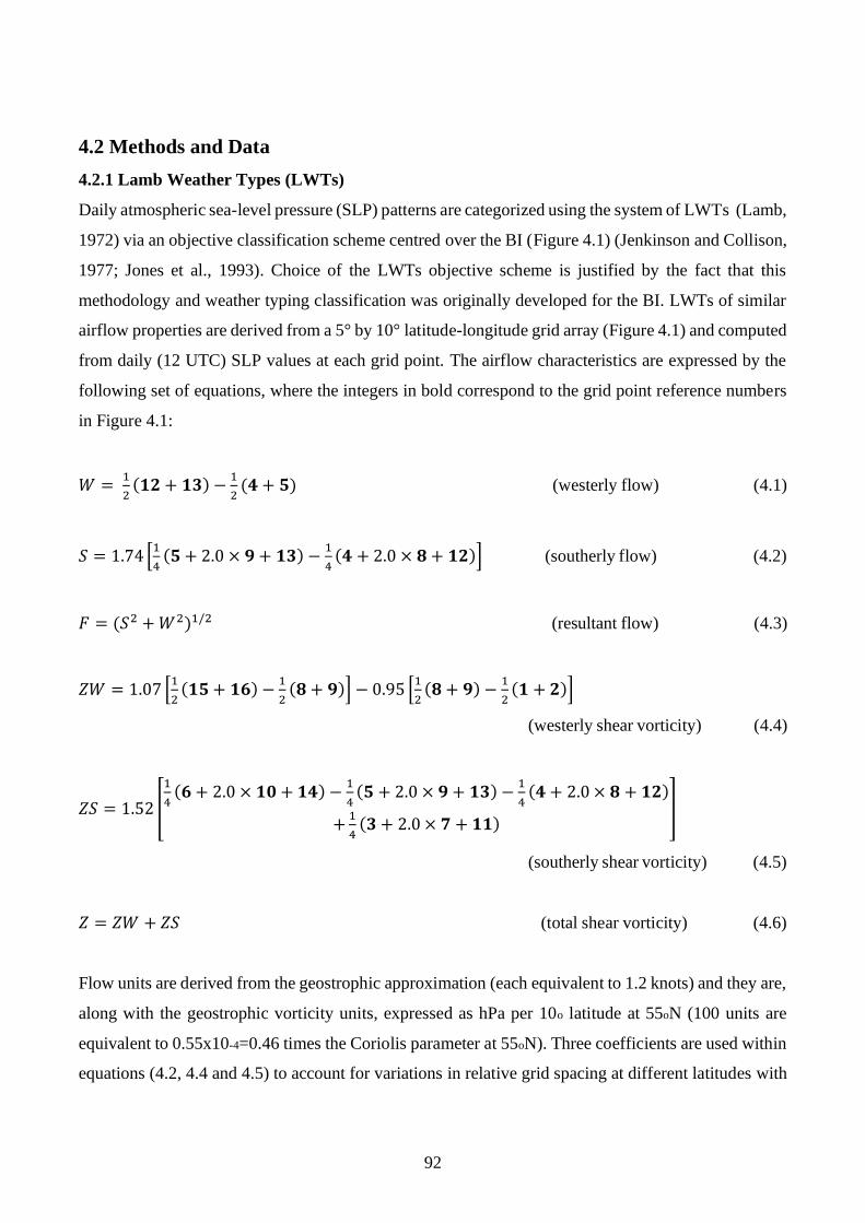
92

4.2 Methods and Data

4.2.1 Lamb Weather Types (LWTs)

Daily atmospheric sea-level pressure (SLP) patterns are categorized using the system of LWTs (Lamb,

1972) via an objective classification scheme centred over the BI (Figure 4.1) (Jenkinson and Collison,

1977; Jones et al., 1993). Choice of the LWTs objective scheme is justified by the fact that this

methodology and weather typing classification was originally developed for the BI. LWTs of similar

airflow properties are derived from a 5° by 10° latitude-longitude grid array (Figure 4.1) and computed

from daily (12 UTC) SLP values at each grid point. The airflow characteristics are expressed by the

following set of equations, where the integers in bold correspond to the grid point reference numbers

in Figure 4.1:

𝑊 = 1

2(𝟏𝟐 + 𝟏𝟑) −

1

2(𝟒 + 𝟓) (westerly flow) (4.1)

𝑆 = 1.74 [1

4(𝟓 + 2.0 × 𝟗 + 𝟏𝟑) −

1

4(𝟒 + 2.0 × 𝟖 + 𝟏𝟐)] (southerly flow) (4.2)

𝐹 = (𝑆2 + 𝑊2)1/2 (resultant flow) (4.3)

𝑍𝑊 = 1.07 [1

2(𝟏𝟓 + 𝟏𝟔) −

1

2(𝟖 + 𝟗)] − 0.95 [

1

2(𝟖 + 𝟗) −

1

2(𝟏 + 𝟐)]

(westerly shear vorticity) (4.4)

𝑍𝑆 = 1.52 [

1

4(𝟔 + 2.0 × 𝟏𝟎 + 𝟏𝟒) −

1

4(𝟓 + 2.0 × 𝟗 + 𝟏𝟑) −

1

4(𝟒 + 2.0 × 𝟖 + 𝟏𝟐)

+1

4(𝟑 + 2.0 × 𝟕 + 𝟏𝟏)

]

(southerly shear vorticity) (4.5)

𝑍 = 𝑍𝑊 + 𝑍𝑆 (total shear vorticity) (4.6)

Flow units are derived from the geostrophic approximation (each equivalent to 1.2 knots) and they are,

along with the geostrophic vorticity units, expressed as hPa per 10o latitude at 55oN (100 units are

equivalent to 0.55x10-4=0.46 times the Coriolis parameter at 55oN). Three coefficients are used within

equations (4.2, 4.4 and 4.5) to account for variations in relative grid spacing at different latitudes with

93

latitude (ψ) here set as 55o (Jenkinson and Collison, 1977): S is multiplied by 1.74, derived from 1/cos

(ψ); ZW, 1.07 and 0.95 from sin(ψ)/sin(ψ-5°) and sin(ψ)/sin(ψ+5°); ZS, 1.52 from 1/2(cos(ψ)2).

The last step for defining LWTs is to apply five rules (Jenkinson and Collison, 1977; Jones et al., 1993;

Lamb, 1972):

i) the flow direction is given by tan-1(W/S) and is calculated on an eight-point compass with 45o per

sector. If W is positive, add 180o. Thus, the W-type occurs between 247.5° and 292.5°;

ii) Lamb pure directional weather types (e.g. N, S, or E-types) correspond to an essentially straight

flow, when |Z| is less than F;

iii) Lamb’s pure cyclonic (C) and anticyclonic (A) types are identified when |Z| is greater than 2F,

respectively with Z > 0 and Z < 0;

iv) Lamb’s hybrid types (e.g. AE and CSW) are characterised by a flow partially anticyclonic/cyclonic,

with |Z| lying between F and 2F;

v) the unclassified (U) type is obtained when F and |Z| are less than 6, with the choice of 6 depending

on grid spacing.

The objective classification scheme yields 27 LWTs comprised of two synoptic types (A and C), five

purely directional types (W, NW, E, N, and S) , 19 hybrid combinations of synoptic and directional

types (e.g. CNW, CSE and AE), and 1 unclassified (U) type (Jenkinson and Collison, 1977; Jones et

al., 1993). For persistence and frequency analyses, the focus here is on the 7 synoptic and directional

LWTs plus the U-type. Accordingly, counts of hybrid types were spread across the main types as per

Lamb’s original definition (Lamb, 1972, 1950) and common practice within earlier studies (Hulme et

al., 1993; Jones et al., 2014, 2013, 1993). LWTs persistence and frequency are assessed for summer

(June-July-August, JJA), autumn (September-October-November, SON), winter (December-January-

February, DJF) and spring (March-April-May, MAM). On the other hand, when calculating indices of

future multi-hazards, the hybrid LWTs were not incorporated into the 7 main types as the F-Score and

nocturnal UHI indices require these weather patterns to be considered independently.

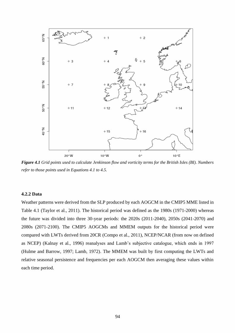
94

Figure 4.1 Grid points used to calculate Jenkinson flow and vorticity terms for the British Isles (BI). Numbers

refer to those points used in Equations 4.1 to 4.5.

4.2.2 Data

Weather patterns were derived from the SLP produced by each AOGCM in the CMIP5 MME listed in

Table 4.1 (Taylor et al., 2011). The historical period was defined as the 1980s (1971-2000) whereas

the future was divided into three 30-year periods: the 2020s (2011-2040), 2050s (2041-2070) and

2080s (2071-2100). The CMIP5 AOGCMs and MMEM outputs for the historical period were

compared with LWTs derived from 20CR (Compo et al., 2011), NCEP/NCAR (from now on defined

as NCEP) (Kalnay et al., 1996) reanalyses and Lamb’s subjective catalogue, which ends in 1997

(Hulme and Barrow, 1997; Lamb, 1972). The MMEM was built by first computing the LWTs and

relative seasonal persistence and frequencies per each AOGCM then averaging these values within

each time period.

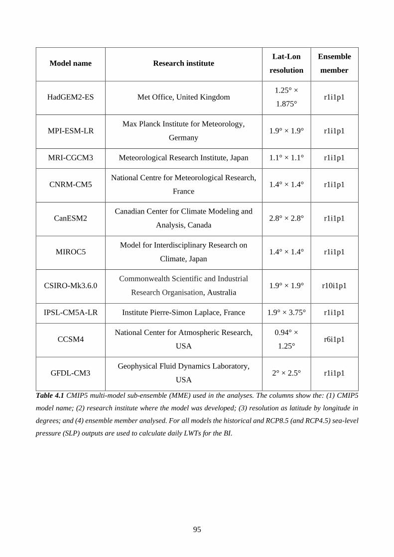
95

Model name Research institute Lat-Lon

resolution

Ensemble

member

HadGEM2-ES Met Office, United Kingdom 1.25° ×

1.875° r1i1p1

MPI-ESM-LR Max Planck Institute for Meteorology,

Germany 1.9° × 1.9° r1i1p1

MRI-CGCM3 Meteorological Research Institute, Japan 1.1° × 1.1° r1i1p1

CNRM-CM5 National Centre for Meteorological Research,

France 1.4° × 1.4° r1i1p1

CanESM2 Canadian Center for Climate Modeling and

Analysis, Canada 2.8° × 2.8° r1i1p1

MIROC5 Model for Interdisciplinary Research on

Climate, Japan 1.4° × 1.4° r1i1p1

CSIRO-Mk3.6.0 Commonwealth Scientific and Industrial

Research Organisation, Australia 1.9° × 1.9° r10i1p1

IPSL-CM5A-LR Institute Pierre-Simon Laplace, France 1.9° × 3.75° r1i1p1

CCSM4 National Center for Atmospheric Research,

USA

0.94° ×

1.25° r6i1p1

GFDL-CM3 Geophysical Fluid Dynamics Laboratory,

USA 2° × 2.5° r1i1p1

Table 4.1 CMIP5 multi-model sub-ensemble (MME) used in the analyses. The columns show the: (1) CMIP5

model name; (2) research institute where the model was developed; (3) resolution as latitude by longitude in

degrees; and (4) ensemble member analysed. For all models the historical and RCP8.5 (and RCP4.5) sea-level

pressure (SLP) outputs are used to calculate daily LWTs for the BI.

96

4.2.3 Persistence and trend analyses

Weather pattern persistence is defined here as the conditional probability (pjj) that a given LWTj on

day(t) is followed by the same LWTj on day(t+1) (Gagniuc, 2017; Wilby, 1994). This diagnostic was

extracted for the 7 main LWTs and the U-type using the diagonal cells of Markov-chain transition

matrices. This enabled estimation of historical (1980s) and future (2020s, 2050s and 2080s) seasonal

persistence for the MMEM as well as for individual AOGCMs for impactful weather types and

seasons, the 20CR, NCEP reanalyses and Lamb’s subjective catalogue.

Uncertainty in pjj for the 1980s was calculated by boot-strapping (n=1,000) 30-year seasonal

simulations using the markovchain package within the R framework (Spedicato, 2017). This algorithm

stochastically generates, with replacement, n series of daily LWTs from the original conditional

distributions of the weather patterns in each AOGCM, then recomputes pjj from each series. The

resulting pBOOTSTRAPjj is the mean of all pjj across the 1000 series, for each AOGCM. The 95%

confidence intervals of pBOOTSTRAPjj are obtained from the cumulative distribution of the 1000 values

of pjj for each AOGCM.

Statistical significance of changes in persistence for the AOGCM sub-ensemble between the 1980s

and future periods was assessed using a Mann-Whitney-Wilcoxon two-tailed test (Mann and Whitney,

1947) applied to the 10 estimates of pBOOTSTRAPjj for each time period. Changes in pjj between the 1980s

and future periods for individual AOGCMs were regarded as statistically significant if future

persistence of a given LWT and AOGCM fell outside the 95% confidence intervals of the pBOOTSTRAPjj

range of that AOGCM for the 1980s.

To detect both linear and non-linear annual changes in the total seasonal counts of LWTs MMEM

frequencies under RCP8.5 and RCP4.5 scenarios, a trend analysis was performed for the 2006-2100

time period. For illustrative purposes, only trends for anticyclonic (A, summer JJA), cyclonic (C,

autumn SON) and westerly (W, winter DJF) types, as indicators of impactful weather across the BI,

are shown. Results are also presented for the southerly (S, spring MAM) types as this LWT shows

most significant changes in seasonal persistence according to the non-parametric Mann-Whitney-

Wilcoxon two-tailed test between the 1980s and each of the three future periods (i.e. 2020s, 2050s and

2080s). A modified Mann-Kendall test, which takes into account possible autocorrelation within the

time series, was applied to both RCP8.5 and RCP4.5 seasonal MMEM LWTs frequencies (Hamed and

Ramachandra Rao, 1998).

97

4.2.4 Indices of winter flood-wind hazards and summer UHI intensity

As a measure of concurrent flood-wind hazards an extended version of the F-Index (De Luca et al.,

2017; Wilby and Quinn, 2013) is here calculated and defined as the F-Score, for each AOGCM,

MMEM, NCEP, 20CR and Lamb’s subjective datasets, covering the 1980s, 2020s, 2050s and 2080s,

for selected LWTs known to drive these multi-hazard events (De Luca et al., 2017) during winter under

both RCP8.5 and RCP4.5. The F-Index is the ratio of observed to expected frequency of floods for a

given LWT, where values greater than 1 show higher than expected likelihood. Ten LWTs are known

to be associated with historic, multi-basin floods (De Luca et al., 2017), of which eight (C, CS, CSW,

CNW, S, SW, W, and NW-types) increase and two (N and A-types) reduce likelihood of multi-basin

flood occurrence. All other LWTs are weighted zero. The F-Score is then calculated by multiplying

the winter DJF frequencies (𝑓𝑟𝑒𝑞_𝑑𝑗𝑓𝑗,𝑖) of these LWTs by their 𝐹_𝐼𝑛𝑑𝑒𝑥𝑗,𝑖 (as per Event Set E in De

Luca et al., 2017) and by summing these values:

𝐹_𝑆𝑐𝑜𝑟𝑒𝑖 = ∑ 𝑓𝑟𝑒𝑞_𝑑𝑗𝑓𝑗,𝑖 𝑥 𝐹_𝐼𝑛𝑑𝑒𝑥𝑗,𝑖 (4.7)

10

𝑗=1

where 𝑖 represents the single AOGCM, NCEP, 20CR and Lamb’s subjective datasets within the

relative time periods of 1980s, 2020s, 2050s, 2080s and 𝑗 is the given LWT considered from the 10

types mentioned above. The higher the F-Score, the greater the likelihood of concurrent multi-basin

flood and wind hazards within winter, over the specified time horizon and RCP scenario.

As a proxy for combined heatwave and poor air quality hazards occurring during summer, observed,

simulated and projected nocturnal UHI temperatures in tenths of degree Celsius for London (UK) are

adopted (Wilby et al., 2011), using the same datasets, time periods and RCPs as per the F-Score. The

UHI phenomenon is caused by absorption and trapping of heat as well as by changed airflows and

sensible heat fluxes within the built environment. The simplest form of UHI metric (used by Wilby et

al., 2011) is based on the daily temperature difference between an urban and rural reference site (during

daylight or night hours). These values may then be stratified by LWT to show the extent to which

some weather patterns favour extreme UHI episodes. The UHI metric was derived as follows by: i)

multiplying LWT summer JJA frequencies (𝑓𝑟𝑒𝑞_𝑗𝑗𝑎ℎ,𝑖) by their respective average UHI intensities

taken from Wilby et al. (2011) (𝑈𝐻𝐼_𝑤ℎ,𝑖); ii) summing these values; and iii) dividing the total from

step ii) by the total number of days in the period analysed (𝑑𝑎𝑦𝑠ℎ,𝑖) to give the mean daily UHI

intensity:

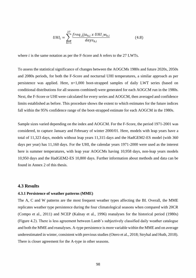
98

𝑈𝐻𝐼𝑖 = ∑𝑓𝑟𝑒𝑞_𝑗𝑗𝑎ℎ,𝑖 𝑥 𝑈𝐻𝐼_𝑤ℎ,𝑖

𝑑𝑎𝑦𝑠ℎ,𝑖

27

ℎ=1

(4.8)

where 𝑖 is the same notation as per the F-Score and ℎ refers to the 27 LWTs.

To assess the statistical significance of changes between the AOGCMs 1980s and future 2020s, 2050s

and 2080s periods, for both the F-Score and nocturnal UHI temperatures, a similar approach as per

persistence was applied. Here, n=1,000 boot-strapped samples of daily LWT series (based on

conditional distributions for all seasons combined) were generated for each AOGCM run in the 1980s.

Next, the F-Score or UHI were calculated for every series and AOGCM, then averaged and confidence

limits established as before. This procedure shows the extent to which estimates for the future indices

fall within the 95% confidence range of the boot-strapped estimate for each AOGCM in the 1980s.

Sample sizes varied depending on the index and AOGCM. For the F-Score, the period 1971-2001 was

considered, to capture January and February of winter 2000/01. Here, models with leap years have a

total of 11,323 days, models without leap years 11,315 days and the HadGEM2-ES model (with 360

days per year) has 11,160 days. For the UHI, the calendar years 1971-2000 were used as the interest

here is summer temperatures, with leap year AOGCMs having 10,958 days, non-leap years models

10,950 days and the HadGEM2-ES 10,800 days. Further information about methods and data can be

found in Annex 2 of this thesis.

4.3 Results

4.3.1 Persistence of weather patterns (MME)

The A, C and W patterns are the most frequent weather types affecting the BI. Overall, the MME

replicates weather type persistence during the four climatological seasons when compared with 20CR

(Compo et al., 2011) and NCEP (Kalnay et al., 1996) reanalyses for the historical period (1980s)

(Figure 4.2). There is less agreement between Lamb’s subjectively classified daily weather catalogue

and both the MME and reanalyses. A-type persistence is more variable within the MME and on average

underestimated in winter, consistent with previous studies (Otero et al., 2018; Stryhal and Huth, 2018).

There is closer agreement for the A-type in other seasons.

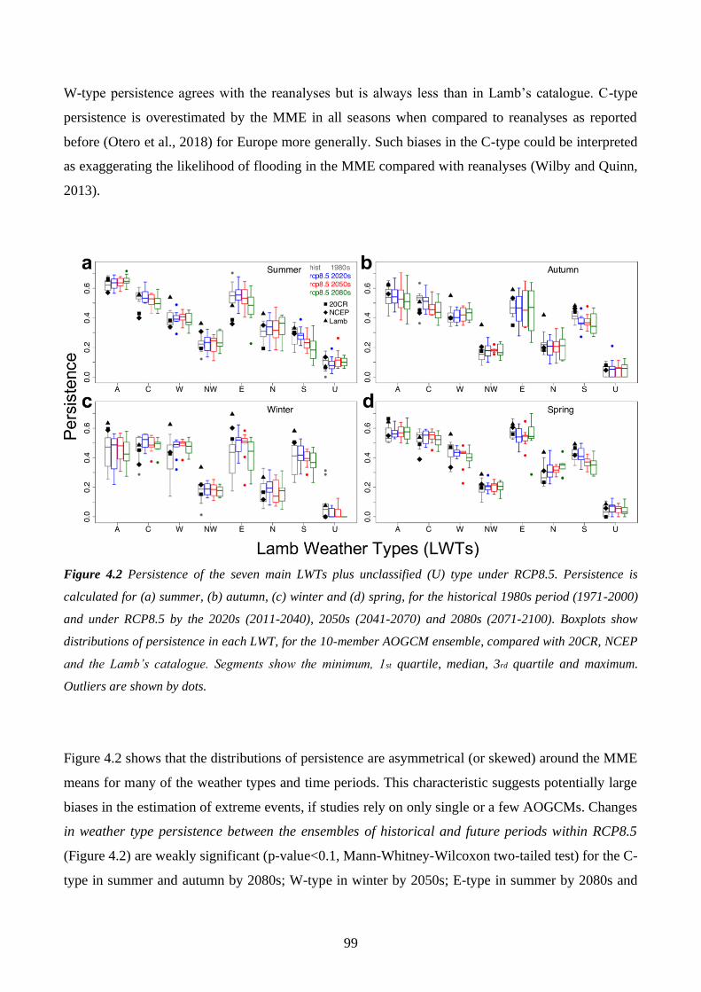
99

W-type persistence agrees with the reanalyses but is always less than in Lamb’s catalogue. C-type

persistence is overestimated by the MME in all seasons when compared to reanalyses as reported

before (Otero et al., 2018) for Europe more generally. Such biases in the C-type could be interpreted

as exaggerating the likelihood of flooding in the MME compared with reanalyses (Wilby and Quinn,

2013).

Figure 4.2 Persistence of the seven main LWTs plus unclassified (U) type under RCP8.5. Persistence is

calculated for (a) summer, (b) autumn, (c) winter and (d) spring, for the historical 1980s period (1971-2000)

and under RCP8.5 by the 2020s (2011-2040), 2050s (2041-2070) and 2080s (2071-2100). Boxplots show

distributions of persistence in each LWT, for the 10-member AOGCM ensemble, compared with 20CR, NCEP

and the Lamb’s catalogue. Segments show the minimum, 1st quartile, median, 3rd quartile and maximum.

Outliers are shown by dots.

Figure 4.2 shows that the distributions of persistence are asymmetrical (or skewed) around the MME

means for many of the weather types and time periods. This characteristic suggests potentially large

biases in the estimation of extreme events, if studies rely on only single or a few AOGCMs. Changes

in weather type persistence between the ensembles of historical and future periods within RCP8.5

(Figure 4.2) are weakly significant (p-value<0.1, Mann-Whitney-Wilcoxon two-tailed test) for the C-

type in summer and autumn by 2080s; W-type in winter by 2050s; E-type in summer by 2080s and

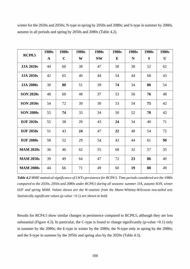
100

winter for the 2020s and 2050s; N-type in spring by 2050s and 2080s; and S-type in summer by 2080s,

autumn in all periods and spring by 2050s and 2080s (Table 4.2).

RCP8.5 1980s

A

1980s

C

1980s

W

1980s

NW

1980s

E

1980s

N

1980s

S

1980s

U

JJA 2020s 44 60 38 47 50 38 52 62

JJA 2050s 42 65 40 44 54 44 68 43

JJA 2080s 30 80 51 39 74 34 80 54

SON 2020s 48 60 48 37 53 56 76 48

SON 2050s 54 72 39 30 53 54 75 42

SON 2080s 55 74 33 34 50 52 78 42

DJF 2020s 55 38 29 43 24 34 40 71

DJF 2050s 51 43 24 47 22 48 54 72

DJF 2080s 58 52 29 54 43 44 61 90

MAM 2020s 36 46 62 55 68 32 57 35

MAM 2050s 39 49 64 47 72 23 86 40

MAM 2080s 44 66 71 49 60 19 88 49

Table 4.2 MME statistical significance of LWTs persistence for RCP8.5. Time periods considered are the 1980s

compared to the 2020s, 2050s and 2080s under RCP8.5 during all seasons: summer JJA, autumn SON, winter

DJF and spring MAM. Values shown are the W-statistic from the Mann-Whitney-Wilcoxon two-tailed test.

Statistically significant values (p-value <0.1) are shown in bold.

Results for RCP4.5 show similar changes in persistence compared to RCP8.5, although they are less

substantial (Figure 4.3). In particular, the C-type is found to change significantly (p-value <0.1) only

in summer by the 2080s; the E-type in winter by the 2080s; the N-type only in spring by the 2080s;

and the S-type in summer by the 2050s and spring also by the 2020s (Table 4.3).

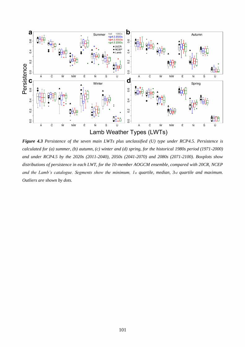
101

Figure 4.3 Persistence of the seven main LWTs plus unclassified (U) type under RCP4.5. Persistence is

calculated for (a) summer, (b) autumn, (c) winter and (d) spring, for the historical 1980s period (1971-2000)

and under RCP4.5 by the 2020s (2011-2040), 2050s (2041-2070) and 2080s (2071-2100). Boxplots show

distributions of persistence in each LWT, for the 10-member AOGCM ensemble, compared with 20CR, NCEP

and the Lamb’s catalogue. Segments show the minimum, 1st quartile, median, 3rd quartile and maximum.

Outliers are shown by dots.

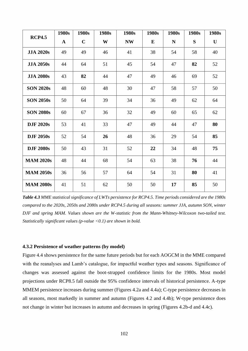
102

RCP4.5 1980s

A

1980s

C

1980s

W

1980s

NW

1980s

E

1980s

N

1980s

S

1980s

U

JJA 2020s 49 49 46 41 38 54 58 40

JJA 2050s 44 64 51 45 54 47 82 52

JJA 2080s 43 82 44 47 49 46 69 52

SON 2020s 48 60 48 30 47 58 57 50

SON 2050s 50 64 39 34 36 49 62 64

SON 2080s 60 67 36 32 49 60 65 62

DJF 2020s 53 41 33 47 49 44 47 80

DJF 2050s 52 54 26 48 36 29 54 85

DJF 2080s 50 43 31 52 22 34 48 75

MAM 2020s 48 44 68 54 63 38 76 44

MAM 2050s 36 56 57 64 54 31 80 41

MAM 2080s 41 51 62 50 50 17 85 50

Table 4.3 MME statistical significance of LWTs persistence for RCP4.5. Time periods considered are the 1980s

compared to the 2020s, 2050s and 2080s under RCP4.5 during all seasons: summer JJA, autumn SON, winter

DJF and spring MAM. Values shown are the W-statistic from the Mann-Whitney-Wilcoxon two-tailed test.

Statistically significant values (p-value <0.1) are shown in bold.

4.3.2 Persistence of weather patterns (by model)

Figure 4.4 shows persistence for the same future periods but for each AOGCM in the MME compared

with the reanalyses and Lamb’s catalogue, for impactful weather types and seasons. Significance of

changes was assessed against the boot-strapped confidence limits for the 1980s. Most model

projections under RCP8.5 fall outside the 95% confidence intervals of historical persistence. A-type

MMEM persistence increases during summer (Figures 4.2a and 4.4a); C-type persistence decreases in

all seasons, most markedly in summer and autumn (Figures 4.2 and 4.4b); W-type persistence does

not change in winter but increases in autumn and decreases in spring (Figures 4.2b-d and 4.4c).

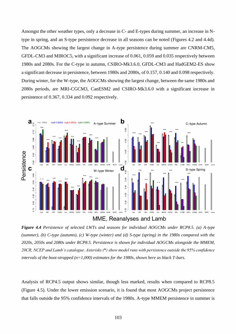
103

Amongst the other weather types, only a decrease in C- and E-types during summer, an increase in N-

type in spring, and an S-type persistence decrease in all seasons can be noted (Figures 4.2 and 4.4d).

The AOGCMs showing the largest change in A-type persistence during summer are CNRM-CM5,

GFDL-CM3 and MIROC5, with a significant increase of 0.061, 0.059 and 0.035 respectively between

1980s and 2080s. For the C-type in autumn, CSIRO-Mk3.6.0, GFDL-CM3 and HadGEM2-ES show

a significant decrease in persistence, between 1980s and 2080s, of 0.157, 0.140 and 0.098 respectively.

During winter, for the W-type, the AOGCMs showing the largest change, between the same 1980s and

2080s periods, are MRI-CGCM3, CanESM2 and CSIRO-Mk3.6.0 with a significant increase in

persistence of 0.367, 0.334 and 0.092 respectively.

Figure 4.4 Persistence of selected LWTs and seasons for individual AOGCMs under RCP8.5. (a) A-type

(summer), (b) C-type (autumn), (c) W-type (winter) and (d) S-type (spring) in the 1980s compared with the

2020s, 2050s and 2080s under RCP8.5. Persistence is shown for individual AOGCMs alongside the MMEM,

20CR, NCEP and Lamb’s catalogue. Asterisks (*) show model runs with persistence outside the 95% confidence

intervals of the boot-strapped (n=1,000) estimates for the 1980s, shown here as black T-bars.

Analysis of RCP4.5 output shows similar, though less marked, results when compared to RCP8.5

(Figure 4.5). Under the lower emission scenario, it is found that most AOGCMs project persistence

that falls outside the 95% confidence intervals of the 1980s. A-type MMEM persistence in summer is

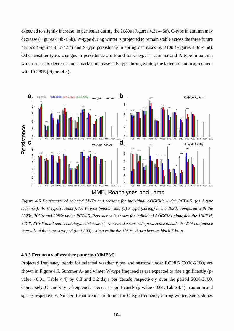
104

expected to slightly increase, in particular during the 2080s (Figures 4.3a-4.5a), C-type in autumn may

decrease (Figures 4.3b-4.5b), W-type during winter is projected to remain stable across the three future

periods (Figures 4.3c-4.5c) and S-type persistence in spring decreases by 2100 (Figures 4.3d-4.5d).

Other weather types changes in persistence are found for C-type in summer and A-type in autumn

which are set to decrease and a marked increase in E-type during winter; the latter are not in agreement

with RCP8.5 (Figure 4.3).

Figure 4.5 Persistence of selected LWTs and seasons for individual AOGCMs under RCP4.5. (a) A-type

(summer), (b) C-type (autumn), (c) W-type (winter) and (d) S-type (spring) in the 1980s compared with the

2020s, 2050s and 2080s under RCP4.5. Persistence is shown for individual AOGCMs alongside the MMEM,

20CR, NCEP and Lamb’s catalogue. Asterisks (*) show model runs with persistence outside the 95% confidence

intervals of the boot-strapped (n=1,000) estimates for the 1980s, shown here as black T-bars.

4.3.3 Frequency of weather patterns (MMEM)

Projected frequency trends for selected weather types and seasons under RCP8.5 (2006-2100) are

shown in Figure 4.6. Summer A- and winter W-type frequencies are expected to rise significantly (p-

value <0.01, Table 4.4) by 0.8 and 0.2 days per decade respectively over the period 2006-2100.

Conversely, C- and S-type frequencies decrease significantly (p-value <0.01, Table 4.4) in autumn and

spring respectively. No significant trends are found for C-type frequency during winter. Sen’s slopes

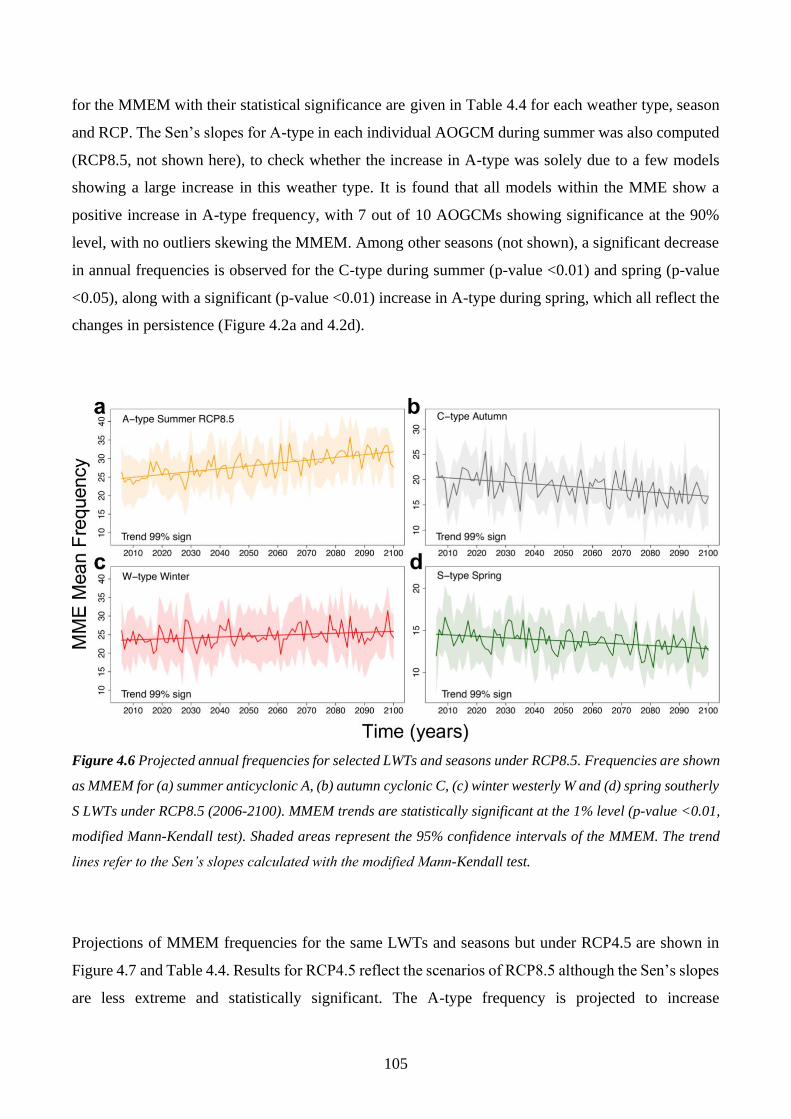
105

for the MMEM with their statistical significance are given in Table 4.4 for each weather type, season

and RCP. The Sen’s slopes for A-type in each individual AOGCM during summer was also computed

(RCP8.5, not shown here), to check whether the increase in A-type was solely due to a few models

showing a large increase in this weather type. It is found that all models within the MME show a

positive increase in A-type frequency, with 7 out of 10 AOGCMs showing significance at the 90%

level, with no outliers skewing the MMEM. Among other seasons (not shown), a significant decrease

in annual frequencies is observed for the C-type during summer (p-value <0.01) and spring (p-value

<0.05), along with a significant (p-value <0.01) increase in A-type during spring, which all reflect the

changes in persistence (Figure 4.2a and 4.2d).

Figure 4.6 Projected annual frequencies for selected LWTs and seasons under RCP8.5. Frequencies are shown

as MMEM for (a) summer anticyclonic A, (b) autumn cyclonic C, (c) winter westerly W and (d) spring southerly

S LWTs under RCP8.5 (2006-2100). MMEM trends are statistically significant at the 1% level (p-value <0.01,

modified Mann-Kendall test). Shaded areas represent the 95% confidence intervals of the MMEM. The trend

lines refer to the Sen’s slopes calculated with the modified Mann-Kendall test.

Projections of MMEM frequencies for the same LWTs and seasons but under RCP4.5 are shown in

Figure 4.7 and Table 4.4. Results for RCP4.5 reflect the scenarios of RCP8.5 although the Sen’s slopes

are less extreme and statistically significant. The A-type frequency is projected to increase

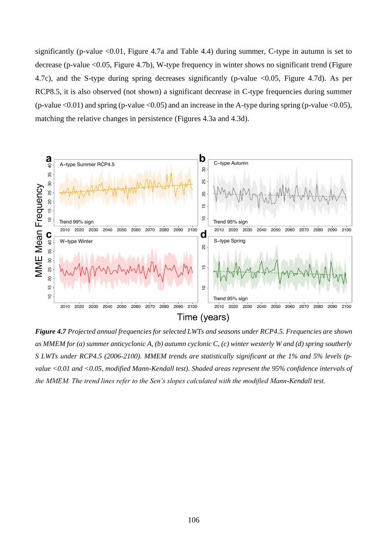
106

significantly (p-value <0.01, Figure 4.7a and Table 4.4) during summer, C-type in autumn is set to

decrease (p-value <0.05, Figure 4.7b), W-type frequency in winter shows no significant trend (Figure

4.7c), and the S-type during spring decreases significantly (p-value <0.05, Figure 4.7d). As per

RCP8.5, it is also observed (not shown) a significant decrease in C-type frequencies during summer

(p-value <0.01) and spring (p-value <0.05) and an increase in the A-type during spring (p-value <0.05),

matching the relative changes in persistence (Figures 4.3a and 4.3d).

Figure 4.7 Projected annual frequencies for selected LWTs and seasons under RCP4.5. Frequencies are shown

as MMEM for (a) summer anticyclonic A, (b) autumn cyclonic C, (c) winter westerly W and (d) spring southerly

S LWTs under RCP4.5 (2006-2100). MMEM trends are statistically significant at the 1% and 5% levels (p-

value <0.01 and <0.05, modified Mann-Kendall test). Shaded areas represent the 95% confidence intervals of

the MMEM. The trend lines refer to the Sen’s slopes calculated with the modified Mann-Kendall test.

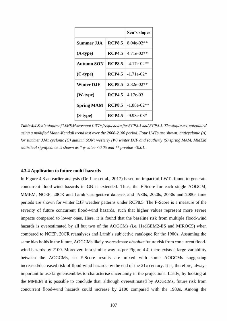
107

Sen’s slopes

Summer JJA

(A-type)

RCP8.5 8.04e-02**

RCP4.5 4.71e-02**

Autumn SON

(C-type)

RCP8.5 -4.17e-02**

RCP4.5 -1.71e-02*

Winter DJF

(W-type)

RCP8.5 2.32e-02**

RCP4.5 4.17e-03

Spring MAM

(S-type)

RCP8.5 -1.88e-02**

RCP4.5 -9.93e-03*

Table 4.4 Sen’s slopes of MMEM seasonal LWTs frequencies for RCP8.5 and RCP4.5. The slopes are calculated

using a modified Mann-Kendall trend test over the 2006-2100 period. Four LWTs are shown: anticyclonic (A)

for summer JJA; cyclonic (C) autumn SON; westerly (W) winter DJF and southerly (S) spring MAM. MMEM

statistical significance is shown as * p-value <0.05 and ** p-value <0.01.

4.3.4 Application to future multi-hazards

In Figure 4.8 an earlier analysis (De Luca et al., 2017) based on impactful LWTs found to generate

concurrent flood-wind hazards in GB is extended. Thus, the F-Score for each single AOGCM,

MMEM, NCEP, 20CR and Lamb’s subjective datasets and 1980s, 2020s, 2050s and 2080s time

periods are shown for winter DJF weather patterns under RCP8.5. The F-Score is a measure of the

severity of future concurrent flood-wind hazards, such that higher values represent more severe

impacts compared to lower ones. Here, it is found that the baseline risk from multiple flood-wind

hazards is overestimated by all but two of the AOGCMs (i.e. HadGEM2-ES and MIROC5) when

compared to NCEP, 20CR reanalyses and Lamb’s subjective catalogue for the 1980s. Assuming the

same bias holds in the future, AOGCMs likely overestimate absolute future risk from concurrent flood-

wind hazards by 2100. Moreover, in a similar way as per Figure 4.4, there exists a large variability

between the AOGCMs, so F-Score results are mixed with some AOGCMs suggesting

increased/decreased risk of flood-wind hazards by the end of the 21st century. It is, therefore, always

important to use large ensembles to characterise uncertainty in the projections. Lastly, by looking at

the MMEM it is possible to conclude that, although overestimated by AOGCMs, future risk from

concurrent flood-wind hazards could increase by 2100 compared with the 1980s. Among the

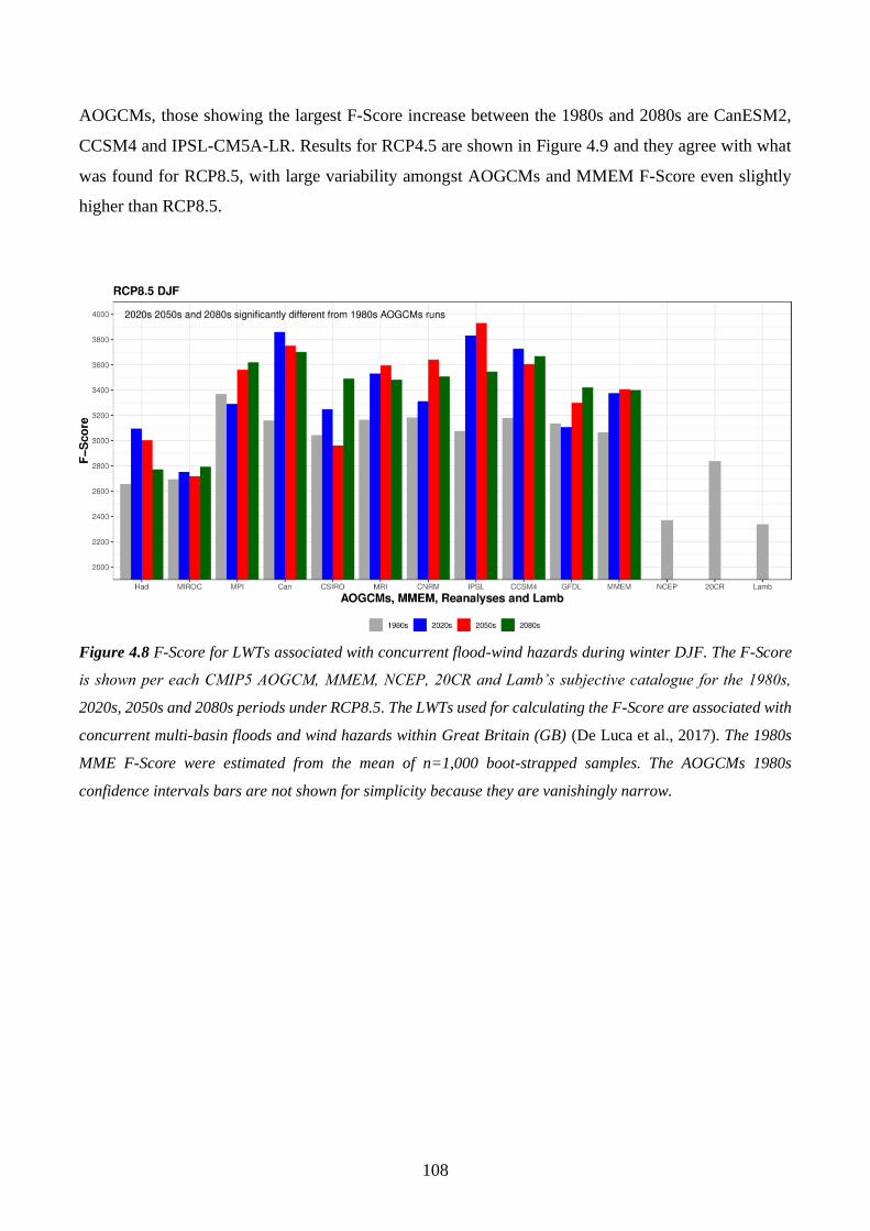
108

AOGCMs, those showing the largest F-Score increase between the 1980s and 2080s are CanESM2,

CCSM4 and IPSL-CM5A-LR. Results for RCP4.5 are shown in Figure 4.9 and they agree with what

was found for RCP8.5, with large variability amongst AOGCMs and MMEM F-Score even slightly

higher than RCP8.5.

Figure 4.8 F-Score for LWTs associated with concurrent flood-wind hazards during winter DJF. The F-Score

is shown per each CMIP5 AOGCM, MMEM, NCEP, 20CR and Lamb’s subjective catalogue for the 1980s,

2020s, 2050s and 2080s periods under RCP8.5. The LWTs used for calculating the F-Score are associated with

concurrent multi-basin floods and wind hazards within Great Britain (GB) (De Luca et al., 2017). The 1980s

MME F-Score were estimated from the mean of n=1,000 boot-strapped samples. The AOGCMs 1980s

confidence intervals bars are not shown for simplicity because they are vanishingly narrow.

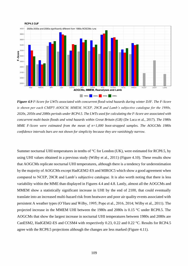
109

Figure 4.9 F-Score for LWTs associated with concurrent flood-wind hazards during winter DJF. The F-Score

is shown per each CMIP5 AOGCM, MMEM, NCEP, 20CR and Lamb’s subjective catalogue for the 1980s,

2020s, 2050s and 2080s periods under RCP4.5. The LWTs used for calculating the F-Score are associated with

concurrent multi-basin floods and wind hazards within Great Britain (GB) (De Luca et al., 2017). The 1980s

MME F-Score were estimated from the mean of n=1,000 boot-strapped samples. The AOGCMs 1980s

confidence intervals bars are not shown for simplicity because they are vanishingly narrow.

Summer nocturnal UHI temperatures in tenths of °C for London (UK), were estimated for RCP8.5, by

using UHI values obtained in a previous study (Wilby et al., 2011) (Figure 4.10). These results show

that AOGCMs replicate nocturnal UHI temperatures, although there is a tendency for underestimation

by the majority of AOGCMs except HadGEM2-ES and MIROC5 which show a good agreement when

compared to NCEP, 20CR and Lamb’s subjective catalogue. It is also worth noting that there is less

variability within the MME than displayed in Figures 4.4 and 4.8. Lastly, almost all the AOGCMs and

MMEM show a statistically significant increase in UHI by the end of 2100, that could eventually

translate into an increased multi-hazard risk from heatwave and poor air quality events associated with

persistent A weather types (O’Hare and Wilby, 1995; Pope et al., 2016, 2014; Wilby et al., 2011). The

projected increase in the MMEM UHI between the 1980s and 2080s is 0.15 °C under RCP8.5. The

AOGCMs that show the largest increase in nocturnal UHI temperatures between 1980s and 2080s are

CanESM2, HadGEM2-ES and CCSM4 with respectively 0.23, 0.22 and 0.22 °C. Results for RCP4.5

agree with the RCP8.5 projections although the changes are less marked (Figure 4.11).

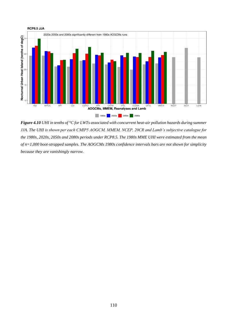
110

Figure 4.10 UHI in tenths of °C for LWTs associated with concurrent heat-air pollution hazards during summer

JJA. The UHI is shown per each CMIP5 AOGCM, MMEM, NCEP, 20CR and Lamb’s subjective catalogue for

the 1980s, 2020s, 2050s and 2080s periods under RCP8.5. The 1980s MME UHI were estimated from the mean

of n=1,000 boot-strapped samples. The AOGCMs 1980s confidence intervals bars are not shown for simplicity

because they are vanishingly narrow.

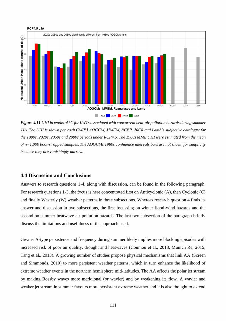
111

Figure 4.11 UHI in tenths of °C for LWTs associated with concurrent heat-air pollution hazards during summer

JJA. The UHI is shown per each CMIP5 AOGCM, MMEM, NCEP, 20CR and Lamb’s subjective catalogue for

the 1980s, 2020s, 2050s and 2080s periods under RCP4.5. The 1980s MME UHI were estimated from the mean

of n=1,000 boot-strapped samples. The AOGCMs 1980s confidence intervals bars are not shown for simplicity

because they are vanishingly narrow.

4.4 Discussion and Conclusions

Answers to research questions 1-4, along with discussion, can be found in the following paragraph.

For research questions 1-3, the focus is here concentrated first on Anticyclonic (A), then Cyclonic (C)

and finally Westerly (W) weather patterns in three subsections. Whereas research question 4 finds its

answer and discussion in two subsections, the first focussing on winter flood-wind hazards and the

second on summer heatwave-air pollution hazards. The last two subsection of the paragraph briefly

discuss the limitations and usefulness of the approach used.

Greater A-type persistence and frequency during summer likely implies more blocking episodes with

increased risk of poor air quality, drought and heatwaves (Coumou et al., 2018; Munich Re, 2015;

Tang et al., 2013). A growing number of studies propose physical mechanisms that link AA (Screen

and Simmonds, 2010) to more persistent weather patterns, which in turn enhance the likelihood of

extreme weather events in the northern hemisphere mid-latitudes. The AA affects the polar jet stream

by making Rossby waves more meridional (or wavier) and by weakening its flow. A wavier and

weaker jet stream in summer favours more persistent extreme weather and it is also thought to extend

112

ridges northward, enhancing such effects (Cohen et al., 2014; Coumou et al., 2018; Francis and Skific,

2015; Francis, 2017; Francis et al., 2017; Francis and Vavrus, 2012; Tang et al., 2013). Diverse studies

shown that the jet stream, since 1979, has become wavier (e.g. Coumou et al., 2018; Di Capua and

Coumou, 2016).

The results found in Chapter 4 support earlier analysis (Otero et al., 2018), and are consistent with the

proposed mechanisms linking observed AA with mid-latitude weather extremes. On the other hand,

AA is expected to have limited effect on simulated CMIP5 blocking over Eurasia under RCP8.5 in the

second half of the 21st century (Woollings et al., 2014). Other work also shows an overall decrease in

CMIP5 blocking events over the BI in winter DJF and summer JJA, during 2061-2090 (RCP8.5)

(Woollings et al., 2018). The findings for anticyclonic weather appear to contradict this. Although A-

type persistence and frequency are not the same as blocking, there was an expectation that the studies

to agree as both mechanisms involve high pressure weather patterns. The only common denominator

between the findings and the studies on blocking (Woollings et al., 2018, 2014) seems to be the

underestimation of A-type/blocking events by CMIP5 models. Further research is needed to reconcile

these apparently contradictory findings. Possible explanations are that results depend on the exact

spatial domain and/or suite of AOGCMs analysed in each MME, as well as on the methodology used

to define A-type days and blocking events.

Less persistent C-types in autumn suggests lower likelihood of heavy rainfall, with reduced recharge

of soil moisture and aquifers at the start of the hydrological year favouring winter droughts. Fewer

cyclonic days may also translate into less frequent severe gales and flooding episodes (Wilby and

Quinn, 2013), as in GB extreme multi-basin flooding events are strongly associated with C-type

weather over time windows from 1 to 19 days (De Luca et al., 2017). Conversely, more frequent zonal

airflow (W-type) in winter may counteract some loss of precipitation from the C-type, especially

across higher elevation regions of the north and west BI where there is strong orographic enhancement

(Burt and Howden, 2013). Such changes may be attributed to AA, however, the physical mechanisms

linking AA to changes in northern hemisphere mid-latitude circulation currently remains an open

question.

From the analyses it is also possible to infer future changes with respect to multi-hazards (Gill and

Malamud, 2014; Zscheischler et al., 2018), through the F-Score and nocturnal UHI temperatures

(research question 4). In Chapter 3 it is shown that in GB multi-basin flooding and extreme wind events

are driven by LWTs mainly associated with C- and W-types (De Luca et al., 2017). These multi-hazard

113

events can generate significant economic losses, hence projections of such events may help in

evaluating future risks and in improving resilience. It is shown that during winter DJF the AOGCMs

overestimate the F-Score when compared to NCEP, 20CR reanalyses and Lamb’s subjective dataset.

Even so, by the end of 2100 the MMEM shows a statistically significant increase in the F-Score

compared with the 1980s within those same models, suggesting that the risk of concurrent flood-wind

impacts may become more severe in a warmer world.

Nocturnal UHI temperatures in London modelled by AOGCMs agree with NCEP, 20CR and Lamb’s

subjective datasets, although they are slightly underestimated for the 1980s. Nocturnal UHI severity

is expected to increase by 2100 under RCP8.5 (MMEM). The results confirm an increasing trend of

~0.3 °C in nocturnal UHI in London found in an earlier study over the observational period 1950-2006

(Wilby et al., 2011). The findings are also in line with the UK Climate Projections Science Report

2009 (Murphy et al., 2009) which suggests that intense UHI events are highly correlated with A-type

weather patterns, and that in London, intense UHI summer events are expected to become more severe

in the future (Wilby, 2008). However, further analysis of projections of UHI is needed with a larger

model ensemble to better account for uncertainty. These present findings, when coupled with a

significant increase in persistence and frequency of A-type weather pattern, suggests a combined

increased risk of heatwaves and poor air quality events in London (O’Hare and Wilby, 1995; Pope et

al., 2016, 2014; Wilby, 2008; Wilby et al., 2011) that could negatively impact human health.

Finally, it is illustrated how changes in the persistence and frequency of weather patterns are useful

diagnostics of climate model realism and can translate into regional to local weather and climate risks

scenarios, which could be helpful for developing narratives for decision-makers. However, caution

needs to be taken when qualitatively converting synoptic weather pattern changes into local variability

because AOGCM skill in reproducing climatic variables at local scales varies significantly and is not

always consistent with observations. This is particularly true for precipitation where, for example,

pressure fields alone are not able to provide reliable local projections (Murawski et al., 2016).

With the UK Climate Projections 2018 partly released and the third UK Climate Change Risk

Assessment now underway, weather pattern analysis could help to both evaluate the new projections

and offer ways of explaining changes that are intelligible to a range of user communities. Similar links

to persistence could be made in other regions with established weather pattern typologies, such as the

Grosswetterlagen for Europe (Hess and Brezowsky, 1952), hydrologically important weather types in

114

the contiguous United States (Prein et al., 2019) and Spatial Synoptic Classification for North America

(Kalkstein et al., 1996).

4.5 Summary

In the above chapter, an investigation of observed, simulated and projected weather patterns (or Lamb

Weather Types, LWTs) (Jones et al., 1993; Lamb, 1972) over the British Isles (BI) is presented (De

Luca et al., 2019a). Specifically, the focus was on the quantification of LWTs frequency and

persistence, by evaluating how well the latter is simulated by a sub-ensemble of CMIP5 models (Taylor

et al., 2011) and how this might change in the future under two RCP scenarios (RCPs 8.5 and 4.5).

Furthermore, associated multi-hazards, driven by LWTs, were also addressed from both the

quantitative and qualitative perspectives. Results show that CMIP5 models are generally able to

reproduce LWTs persistence when compared to NCEP and 20CR reanalyses, with the anticyclonic (A)

and cyclonic (C) weather types respectively underestimated and overestimated. The A-types are set to

increase by 2100, during summer, in both frequency and persistence. The C-types, on the other hand,

may decrease in the future during autumn. This translates into an enhanced (decreased) risk of

heatwave, drought and air pollution (flooding and storm) events. With respect to multi-hazards, the

computation of the F-Score, an index that quantifies the impacts of concurrent flood and storms events,

shows that the CMIP5 models overestimate it during winter, but nonetheless the index is set to increase

in the future. The summer nocturnal Urban Heat Island (UHI) temperatures for London (UK) were

also computed (Wilby, 2008; Wilby et al., 2011) and results show that the UHI is slightly

underestimated by CMIP5 models and expected to intensify by 2100. These results could signify an

enhanced risk of concurrent flood-storm and heatwave-air pollution events respectively during winter

and summer by 2100. The analyses were performed for the British Isles and London, however, they

could also be applied in other regions and cities within the mid-latitudes and beyond.

In the next Chapter the geographical region under consideration is extended further and a diverse set

of concurrent hydroclimatic hazards are analysed. Hence, Chapter 5 quantifies concurrent wet and dry

hydrological extremes at the global scale and link these to modes of climate variability (De Luca et

al., 2019c). The analysis is based on the Palmer Drought Severity Index (PDSI) (Dai et al., 2004;

Palmer, 1965) over the 1950-2014 period and climate indices used are the El Niño–Southern

Oscillation (ENSO) (Rayner et al., 2003; Trenberth, 1997), Pacific Decadal Oscillation (PDO)

(Mantua and Hare, 2002) and American Multi-decadal Oscillation (AMO) (Schlesinger and

115

Ramankutty, 1994). Similarly as per Chapters 3-4, Chapter 5 introduces new metrics specifically used

for assessing spatio-temporal joint occurrences of hydroclimatic hazards. Furthermore, Chapter 5

shows the most impactful (i.e. geographically widespread) concurrent flood and drought events, and

it lays the bases for future climate modelling studies, similar to the ones presented in Chapter 4.

116

Chapter 5

Concurrent wet and dry hydrological extremes

at the global scale

5.1 Introduction

As mentioned in previous Chapters, hazards can interact in diverse ways, leading to multi-hazard

events that can exacerbate disaster losses when compared to single-hazard occurrences (Zscheischler

et al., 2018). Such combination of perils can lead to situations beyond the worst-case scenario planned

by emergency managers, (re)insurance companies, businesses and governments. Thus, multi-hazard

events present a critical challenge for disaster risk reduction, as demonstrated for example by the 2010

Russian heatwave (Barriopedro et al., 2011; Zscheischler et al., 2018). The relevance of multi-hazards

has been recognised by both the scientific and stakeholder communities – both have devoted

significant efforts to the topic over the past decade, achieving a significant review with linked socio-

economic implications of multi-hazard events (e.g. Forzieri et al., 2016; Gallina et al., 2016; Gill and

Malamud, 2014; Kappes et al., 2012a; Leonard et al., 2014; Terzi et al., 2019; Tilloy et al., 2019;

UNDRR, 2015; Zscheischler et al., 2018).

Analysis of multi-hazards is highly relevant given anthropogenic climate change. Events such as floods

and droughts already have significant socio-economic impacts (Barredo, 2007; Jonkman, 2005;

Naumann et al., 2015; Zhang et al., 2011), and are expected to become more frequent and/or severe in

the future (Dai, 2012, 2011a; Hirabayashi et al., 2013; Milly et al., 2002), although there exist

uncertainties about whether these projected increases are caused by anthropogenic forcing. Numerous

studies have investigated the combination of flood and drought events or, more generally, wet and dry

hydrological extremes at local and regional scales, for both present and future climates (e.g. Berton et

al., 2017; Collet et al., 2018; Deangelis et al., 1984; Di Baldassarre et al., 2017; Gil-Guirado et al.,

2016; Oni et al., 2016; Parry et al., 2013; Pechlivanidis et al., 2017; Quesada-Montano et al., 2018;

Yan et al., 2013; Yoon et al., 2018). Examples include the analysis of abrupt drought-flood transitions

in China (Yan et al., 2013) and in England and Wales (Parry et al., 2013), the dynamical interplay

between society and hydrological extremes (Di Baldassarre et al., 2017) and indices assessing the long-

term evolution of vulnerability and adaptation to floods and droughts (Gil-Guirado et al., 2016). Other

studies consider wet-dry interactions from a statistical perspective (Collet et al., 2018), or have related

117

these two hazards to large-scale modes of climate variability (Cai and Rensch, 2012; Lee et al., 2018;

Nobre et al., 2017; Siegert et al., 2001; Ward et al., 2014b; Yoon et al., 2018).

Quantifying wet and dry (also extreme) hydrological events at both regional and global scales is a non-

trivial task. Some of the best indicators include the Palmer Drought Severity Index (PDSI) (Dai et al.,

2004; Palmer, 1965), the Standardized Precipitation Index (SPI) (McKee T.B., Doesken N.J., 1995;

McKee et al., 1993) and the Standardized Precipitation Evapotranspiration Index (SPEI) (Vicente-

Serrano et al., 2010). For instance, the PDSI was used to evaluate the combined effect of the Pacific

Decadal Oscillation (PDO) and El Niño Southern Oscillation (ENSO) on global wet and dry changes

over land, showing that when these two modes are in phase (e.g. El Niño-warm PDO) wet and dry

events are amplified (Wang et al., 2014). The PDSI and SPEI have also been used to quantify wet and

dry trends over China (Rubel and Kottek, 2010), with a generally good agreement between the two

(Chen et al., 2017). At the global scale, the SPI and SPEI were used to explore wet and dry links with

ENSO, PDO and the North Atlantic Oscillation (NAO) (Sun et al., 2016). The study found that ENSO

has the greatest spatial impact for wet and dry changes, followed by the PDO having an effect in the

American continent and eastern Russia, and the NAO affecting Europe as well as north Africa. Lastly,

the SPI was also used in a global multi-model ensemble study of future projections in pluvial and

drought events (Martin, 2018). This revealed that more severe pluvial events are expected in already

wet regions and the same applies for more severe drought conditions in dry areas.

In this chapter, a relatively broad definition of multi-hazard events was adopted, including both the

temporal (yet spatially separate) co-occurrence of wet and dry hydrological extremes at the global

scale, and the rapid succession of hydrological extremes of opposite sign at the same location. It is

worth emphasising that the term “hydrological extreme” does not necessarily imply observed flooding

or drought events, unless explicitly mentioned, but simply hydrological observations exceeding a given

threshold (hence extremes). The relevance of both types of hazards is evident. Stakeholders with

geographically diverse portfolios, such as international corporations and (re)insurance companies,

need to have a robust understanding of the co-occurrence statistics of natural hazards, because for

example their supply chains can be obstructed by such events. They also need to account for the

occurrence of damaging events in rapid succession, whose compound impacts may exceed the linear

sum of the expected impacts for isolated wet and dry extremes. Similarly, estimates of the range of

times that intervene between the two different extremes can inform emergency preparedness and

prevention measures. Finally, national economies that are sensitive to agricultural output can be

118

impacted by the occurrence of sequential hydrological extremes (Zampieri et al., 2017; Zhang et al.,

2015).

Notwithstanding their socio-economic relevance, concurrent wet and dry hydrological extreme events

at the global scale have seldom been addressed in the literature. One early study did consider

combinations of wet and dry extremes via observed PDSI for two thresholds (wet, PDSI > 3 and dry,

PDSI < -3) (Dai et al., 2004). This showed that the total global land area (60°S-75°N) impacted by

wet-dry extremes increased between 1950 and 2002, with marked changes occurring from the early

1970s and surface warming being attributed as the cause of these changes after the mid-1980s. This

analysis has been extended in this chapter by: i) using an updated time series (1950-2014); ii)

introducing new metrics for assessing concurrent wet-dry extremes; iii) presenting findings at monthly

rather than annual resolution; and above all iv) defining the most geographically-widespread, but not

necessarily contiguous, multi-hazard events, occurring within each month, instead of simply

considering extreme observations with PDSI > 3 and PDSI < -3. These multi-hazard properties have

been explored using the monthly self-calibrated PDSI dataset (Dai, 2017; Sheffield et al., 2012).

Specifically, the following questions are addressed:

1) How observed globally independent and concurrent wet-dry hydrological extreme events

changed in the past?

2) What were the most spatially extensive independent and concurrent wet-dry hydrological

extreme events?

3) How new metrics can help in better investigate concurrent wet-dry extremes?

4) How are these extremes related to different modes of climate variability?

In Section 5.2 the datasets, algorithm for computing the extreme events, new metrics and correlation

with climate indices are described, along with their relevant statistical tests. Results are presented in

Section 5.3. Thus, the land area impacted by the extreme events is shown in Section 5.3.1 (research

question 1) and the most geographically-widespread events in Section 5.3.2 (research question 2).

Results obtained from the new metrics and correlations with climate indices can be found in Sections

5.3.3-5.3.5, respectively answering research questions 3-4. Lastly, Section 5.4 provides the general

discussion and conclusions, before a summary of the chapter is provided in Section 5.5.

119

5.2 Data and Methods

5.2.1 Data

The self-calibrated monthly-mean Palmer Drought Severity Index based on the Penman-Monteith

model (sc_PDSI_pm) (Dai, 2017; Sheffield et al., 2012) for the 1950-2014 period, at 2.5° horizontal

resolution, was used. Self-calibration enables a more consistent comparison between different climatic

regions, and the Penman-Monteith model outperforms the original PDSI Thornthwaite algorithm

(Wells et al., 2004) in representing potential evaporation at the global scale (Sheffield et al., 2012).

From this dataset, extreme wet and dry monthly observed events have been obtained, by filtering the

data respectively for sc_PDSI_pm ≥ 3 and sc_PDSI_pm ≤ -3. These two thresholds represent very

moist spells and severe droughts. Only grid-cells with time series having ≥ 95% of observations over

the period of interest are considered.

Three climate modes of variability known to affect regional and global precipitation patterns have been

further analysed: the Niño3.4 (Rayner et al., 2003; Trenberth, 1997), PDO (Mantua and Hare, 2002)

and Atlantic Multidecadal Oscillation (AMO) (Schlesinger and Ramankutty, 1994). All these climate

indices are at monthly time-resolution from 1950 to 2014, as issued by the National Oceanic &

Atmospheric Administration (NOAA). These climate indices have been chosen because they are the

ones with largest geographical impacts, also in very-highly populated areas, i.e. North America and

Europe. Other indices, such as the NAO (Barnston and Livezey, 1987), Pacific-North American (PNA)

pattern (Barnston and Livezey, 1987) and Quasi-Biennial Oscillation (QBO) (Baldwin et al., 2001)

have been also tested.

5.2.2 Methods for identifying extreme wet, dry, neutral and wet-dry events

First, the percentage of total land area impacted by the most widespread monthly extreme wet

(sc_PDSI_pm ≥ 3) and dry (sc_PDSI_pm ≤ -3) hydrological events along with neutral (-3 <

sc_PDSI_pm < 3) and extreme wet plus extreme dry events within the period 1950-2014 have been

calculated. Monthly extreme wet events were derived following De Luca et al. (2017) by: (i)

computing the wet annual maxima (AMAX), i.e. the highest sc_PDSI_pm observations within each

calendar year, at each grid-cell, (ii) counting the number of wet AMAX observations by date, and (iii)

taking the extreme wet event with the most geographically-widespread impacts, i.e. largest impacted

area (km2), within each month during 1950-2014.

120

Extreme dry events were calculated in a similar way to extreme wet events except that in place of

AMAX the sc_PDSI_pm annual minima (AMIN), i.e. the lowest sc_PDSI_pm observations within

each year, were used to compute the extreme events. Neutral events were identified as follows: i)

extract the sc_PDSI_pm AMAX of (non-extreme) wet events (0 ≤ sc_PDSI_pm < 3); ii) extract the

sc_PDSI_pm AMIN for (non-extreme) dry events (-3 < sc_PDSI_pm < 0); iii) pool within the same

dataset both (non-extreme) wet/dry AMAX/AMIN events by month; iv) compute the most widespread

neutral events by month as per above. Lastly, concurrent extreme wet-dry events were calculated by

summing their relative impacted areas (%) within each month. A Mann-Kendall test (Kendall, 1975;

Mann, 1945) was performed to assess any significant trends within each time series. Relative Sen’s

slopes (Sen, 1968) with p-values were also computed.

Second, to establish whether the most widespread extreme wet, dry and wet-dry events were solely

due to chance, a boot-strapping analysis of n=10,000 samples was performed from the original

sc_PDSI_pm dataset. The boot-strapping steps were as follows: i) prepare the complete global (i.e. all

grid-cells) sc_PDSI_pm dataset from 1950 to 2014; ii) sample, with replacement, the sc_PDSI_pm

values n=10,000 times from this global dataset; iii) calculate n=10,000 extreme wet and n=10,000

extreme dry events with the same algorithm used above with the original dataset; iv) take the impacted

area of the most geographically-widespread wet and dry events for each sample; v) calculate the mean

and corresponding 95% confidence intervals (c.i.) for the extreme wet and extreme dry events.

Statistical significance was assessed by checking whether observed extreme wet or dry % of total

impacted areas fell outside the 95% c.i. of the boot-strapped means. If this was the case, the

observations were considered statistically significant. This boot-strapping procedure assumes spatial

independence between each grid-cell and therefore it provides, although with replacement, a purely

random output, which is what one can expect from a boot-strapping analysis.

5.2.3 Wet-dry metrics

The wet-dry (WD) ratio is derived on a cell by cell basis by taking the natural logarithm of the total

number of extreme wet observations (months with sc_PDSI_pm ≥ 3) divided by the total number of

extreme dry observations (months with sc_PDSI_pm ≤ -3) over the 1950-2014 period:

𝑊𝐷 − 𝑟𝑎𝑡𝑖𝑜ℎ = ln (∑ 𝑊𝑒𝑡𝑖,ℎ

𝑛𝑖

𝑖=1

∑ 𝐷𝑟𝑦𝑗,ℎ

𝑛𝑗

𝑗=1

⁄ ) (5.1)

121

where ℎ refers to a single grid-cell and 𝑛𝑖 and 𝑛𝑗 are the total number of wet and dry events,

respectively. The WD-ratio gives information about the propensity of a given area to be more affected

by wet or dry extremes. Thus, WD-ratio > 0 signifies that wet extremes outnumber dry extremes and

WD-ratio < 0 indicates a predominance of dry extremes over wet ones. The natural logarithm was used

to narrow the range of WD-ratio values and to separate the wet-dominated versus dry-dominated

regions by sign. As a caveat, it is worth noting that the WD ratio does not account for the different

intensities of wet and dry extremes.

Wet to dry and dry to wet transitions, named extreme transitions (ET) were assessed for each grid-cell

by computing the average time interval (months) between these events, within the 1950-2014 period.

More specifically, ET for wet to dry was derived as follows, for each grid-cell: i) extract both wet

(sc_PDSI_pm ≥ 3) and dry (sc_PDSI_pm ≤ -3) extreme observations from the entire (1950-2014)

sc_PDSI_pm dataset; ii) order observations by time, from oldest to the most recent; iii) retain only the

earliest event in the case of consecutive extreme dry observations and the latest in the case of

consecutive wet observations; iv) calculate the time interval (monthly difference) between wet and dry

observations within the time-series; and v) take the average of the time interval. The same algorithm

was applied for calculating ET from dry to wet for each grid-cell, with the only difference being in

step iii) where the earliest wet and latest dry observations are kept and in step iv) where the time

interval is now calculated between dry to wet transitions.

To check the statistical significance of the observed ET, a boot-strapping analysis with n = 1,000

samples (10,000 samples were not possible due to high computational demand) was performed in a

similar way as for the most widespread extreme wet, dry and wet-dry events. In this analysis, for each

grid-cell, the following steps were followed: i) from the main sc_PDSI_pm dataset extract and flag

extreme wet (sc_PDSI_pm ≥ 3) and extreme dry (sc_PDSI_pm ≤ -3) observations; ii) sample, with

replacement, n=1,000 of these wet and dry observations with the corresponding (sampled) date (year-

month); iii) calculated n=1,000 ET from wet to dry and n=1,000 ET from dry to wet using the same

algorithm as per above; and iv) take the ET (wet to dry and dry to wet) means with the relative 95%

c.i. of the means. Statistical significance was assessed by checking, for each grid-cell, if the observed

ET time interval (wet to dry and dry to wet) mean fell outside the 95% c.i. of the boot-strapped ET

mean. If this was the case the observation was considered statistically significant. Also here, the boot-

strapping assumes spatial independence between grid-cells.

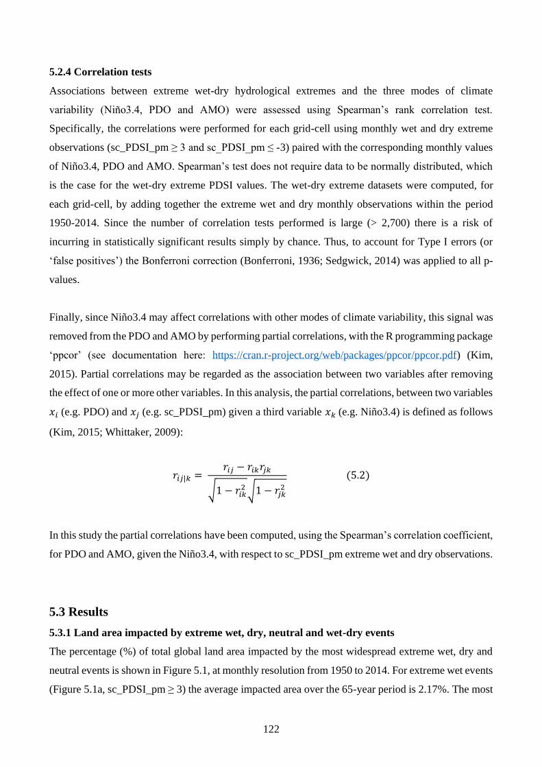
122

5.2.4 Correlation tests

Associations between extreme wet-dry hydrological extremes and the three modes of climate

variability (Niño3.4, PDO and AMO) were assessed using Spearman’s rank correlation test.

Specifically, the correlations were performed for each grid-cell using monthly wet and dry extreme

observations (sc_PDSI_pm ≥ 3 and sc_PDSI_pm ≤ -3) paired with the corresponding monthly values

of Niño3.4, PDO and AMO. Spearman’s test does not require data to be normally distributed, which

is the case for the wet-dry extreme PDSI values. The wet-dry extreme datasets were computed, for

each grid-cell, by adding together the extreme wet and dry monthly observations within the period

1950-2014. Since the number of correlation tests performed is large (> 2,700) there is a risk of

incurring in statistically significant results simply by chance. Thus, to account for Type I errors (or

‘false positives’) the Bonferroni correction (Bonferroni, 1936; Sedgwick, 2014) was applied to all p-

values.

Finally, since Niño3.4 may affect correlations with other modes of climate variability, this signal was

removed from the PDO and AMO by performing partial correlations, with the R programming package

‘ppcor’ (see documentation here: https://cran.r-project.org/web/packages/ppcor/ppcor.pdf) (Kim,

2015). Partial correlations may be regarded as the association between two variables after removing

the effect of one or more other variables. In this analysis, the partial correlations, between two variables

𝑥𝑖 (e.g. PDO) and 𝑥𝑗 (e.g. sc_PDSI_pm) given a third variable 𝑥𝑘 (e.g. Niño3.4) is defined as follows

(Kim, 2015; Whittaker, 2009):

𝑟𝑖𝑗|𝑘 = 𝑟𝑖𝑗 − 𝑟𝑖𝑘𝑟𝑗𝑘

√1 − 𝑟𝑖𝑘2 √1 − 𝑟𝑗𝑘

2

(5.2)

In this study the partial correlations have been computed, using the Spearman’s correlation coefficient,

for PDO and AMO, given the Niño3.4, with respect to sc_PDSI_pm extreme wet and dry observations.

5.3 Results

5.3.1 Land area impacted by extreme wet, dry, neutral and wet-dry events

The percentage (%) of total global land area impacted by the most widespread extreme wet, dry and

neutral events is shown in Figure 5.1, at monthly resolution from 1950 to 2014. For extreme wet events

(Figure 5.1a, sc_PDSI_pm ≥ 3) the average impacted area over the 65-year period is 2.17%. The most

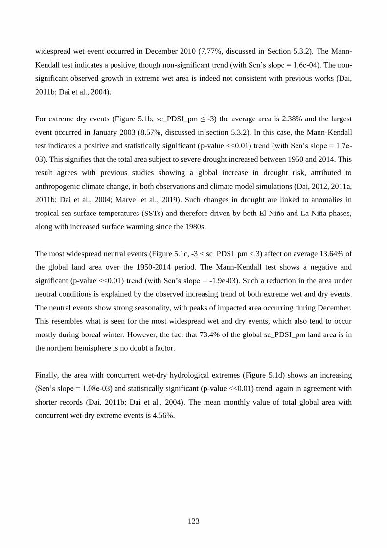
https://cran.r-project.org/web/packages/ppcor/ppcor.pdf

123

widespread wet event occurred in December 2010 (7.77%, discussed in Section 5.3.2). The Mann-

Kendall test indicates a positive, though non-significant trend (with Sen’s slope = 1.6e-04). The non-

significant observed growth in extreme wet area is indeed not consistent with previous works (Dai,

2011b; Dai et al., 2004).

For extreme dry events (Figure 5.1b, sc_PDSI_pm ≤ -3) the average area is 2.38% and the largest

event occurred in January 2003 (8.57%, discussed in section 5.3.2). In this case, the Mann-Kendall

test indicates a positive and statistically significant (p-value <<0.01) trend (with Sen’s slope = 1.7e-

03). This signifies that the total area subject to severe drought increased between 1950 and 2014. This

result agrees with previous studies showing a global increase in drought risk, attributed to

anthropogenic climate change, in both observations and climate model simulations (Dai, 2012, 2011a,

2011b; Dai et al., 2004; Marvel et al., 2019). Such changes in drought are linked to anomalies in

tropical sea surface temperatures (SSTs) and therefore driven by both El Niño and La Niña phases,

along with increased surface warming since the 1980s.

The most widespread neutral events (Figure 5.1c, -3 < sc_PDSI_pm < 3) affect on average 13.64% of

the global land area over the 1950-2014 period. The Mann-Kendall test shows a negative and

significant (p-value <<0.01) trend (with Sen’s slope = -1.9e-03). Such a reduction in the area under

neutral conditions is explained by the observed increasing trend of both extreme wet and dry events.

The neutral events show strong seasonality, with peaks of impacted area occurring during December.

This resembles what is seen for the most widespread wet and dry events, which also tend to occur

mostly during boreal winter. However, the fact that 73.4% of the global sc_PDSI_pm land area is in

the northern hemisphere is no doubt a factor.

Finally, the area with concurrent wet-dry hydrological extremes (Figure 5.1d) shows an increasing

(Sen’s slope = 1.08e-03) and statistically significant (p-value <<0.01) trend, again in agreement with

shorter records (Dai, 2011b; Dai et al., 2004). The mean monthly value of total global area with

concurrent wet-dry extreme events is 4.56%.

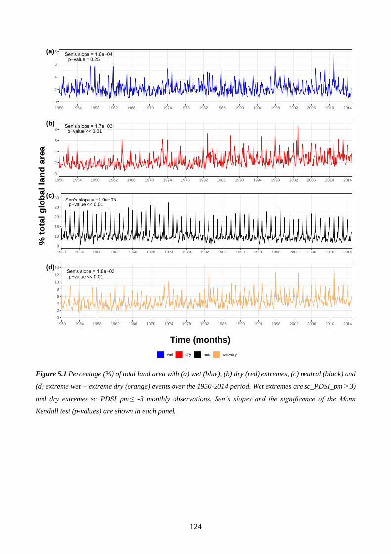
124

Figure 5.1 Percentage (%) of total land area with (a) wet (blue), (b) dry (red) extremes, (c) neutral (black) and

(d) extreme wet + extreme dry (orange) events over the 1950-2014 period. Wet extremes are sc_PDSI_pm ≥ 3)

and dry extremes sc_PDSI_pm ≤ -3 monthly observations. Sen’s slopes and the significance of the Mann

Kendall test (p-values) are shown in each panel.

Sen's slope = 1.6e−04p−value = 0.25

0

2

4

6

8

1950 1954 1958 1962 1966 1970 1974 1978 1982 1986 1990 1994 1998 2002 2006 2010 2014

(a)

Sen's slope = 1.7e−03p−value << 0.01

0

2

4

6

8

1950 1954 1958 1962 1966 1970 1974 1978 1982 1986 1990 1994 1998 2002 2006 2010 2014

(b)

Sen's slope = −1.9e−03p−value << 0.01

8

13

18

23

28

33

1950 1954 1958 1962 1966 1970 1974 1978 1982 1986 1990 1994 1998 2002 2006 2010 2014

(c)

Sen's slope = 1.8e−03p−value << 0.01

0

2

4

6

8

10

12

14

1950 1954 1958 1962 1966 1970 1974 1978 1982 1986 1990 1994 1998 2002 2006 2010 2014

(d)

Time (months)

% t

ota

l g

lob

al

lan

d a

rea

wet dry neu wet−dry

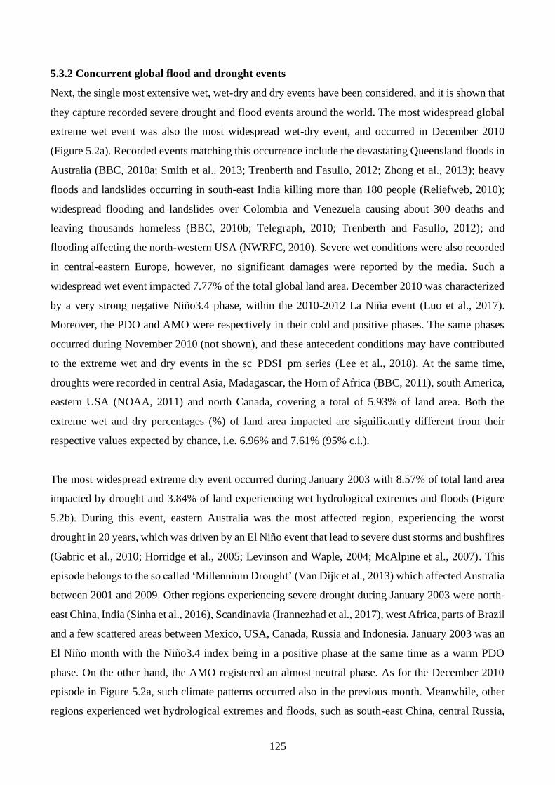
125

5.3.2 Concurrent global flood and drought events

Next, the single most extensive wet, wet-dry and dry events have been considered, and it is shown that

they capture recorded severe drought and flood events around the world. The most widespread global

extreme wet event was also the most widespread wet-dry event, and occurred in December 2010

(Figure 5.2a). Recorded events matching this occurrence include the devastating Queensland floods in

Australia (BBC, 2010a; Smith et al., 2013; Trenberth and Fasullo, 2012; Zhong et al., 2013); heavy

floods and landslides occurring in south-east India killing more than 180 people (Reliefweb, 2010);

widespread flooding and landslides over Colombia and Venezuela causing about 300 deaths and

leaving thousands homeless (BBC, 2010b; Telegraph, 2010; Trenberth and Fasullo, 2012); and

flooding affecting the north-western USA (NWRFC, 2010). Severe wet conditions were also recorded

in central-eastern Europe, however, no significant damages were reported by the media. Such a

widespread wet event impacted 7.77% of the total global land area. December 2010 was characterized

by a very strong negative Niño3.4 phase, within the 2010-2012 La Niña event (Luo et al., 2017).

Moreover, the PDO and AMO were respectively in their cold and positive phases. The same phases

occurred during November 2010 (not shown), and these antecedent conditions may have contributed

to the extreme wet and dry events in the sc_PDSI_pm series (Lee et al., 2018). At the same time,

droughts were recorded in central Asia, Madagascar, the Horn of Africa (BBC, 2011), south America,

eastern USA (NOAA, 2011) and north Canada, covering a total of 5.93% of land area. Both the

extreme wet and dry percentages (%) of land area impacted are significantly different from their

respective values expected by chance, i.e. 6.96% and 7.61% (95% c.i.).

The most widespread extreme dry event occurred during January 2003 with 8.57% of total land area

impacted by drought and 3.84% of land experiencing wet hydrological extremes and floods (Figure

5.2b). During this event, eastern Australia was the most affected region, experiencing the worst

drought in 20 years, which was driven by an El Niño event that lead to severe dust storms and bushfires

(Gabric et al., 2010; Horridge et al., 2005; Levinson and Waple, 2004; McAlpine et al., 2007). This

episode belongs to the so called ‘Millennium Drought’ (Van Dijk et al., 2013) which affected Australia

between 2001 and 2009. Other regions experiencing severe drought during January 2003 were north-

east China, India (Sinha et al., 2016), Scandinavia (Irannezhad et al., 2017), west Africa, parts of Brazil

and a few scattered areas between Mexico, USA, Canada, Russia and Indonesia. January 2003 was an

El Niño month with the Niño3.4 index being in a positive phase at the same time as a warm PDO

phase. On the other hand, the AMO registered an almost neutral phase. As for the December 2010

episode in Figure 5.2a, such climate patterns occurred also in the previous month. Meanwhile, other

regions experienced wet hydrological extremes and floods, such as south-east China, central Russia,

126

Europe, southern Great Britain (BBC, 2003; Marsh, 2004), Madagascar (Reliefweb, 2003), Argentina,

Chile and scattered parts of Africa and Canada (DFO, 2008). The % of land area impacted by both

extreme wet and dry events during January 2003 was significantly different from the value expected

by chance (see above, 95% c.i.).

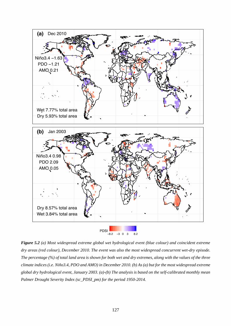
127

Figure 5.2 (a) Most widespread extreme global wet hydrological event (blue colour) and coincident extreme

dry areas (red colour), December 2010. The event was also the most widespread concurrent wet-dry episode.

The percentage (%) of total land area is shown for both wet and dry extremes, along with the values of the three

climate indices (i.e. Niño3.4, PDO and AMO) in December 2010. (b) As (a) but for the most widespread extreme

global dry hydrological event, January 2003. (a)-(b) The analysis is based on the self-calibrated monthly mean

Palmer Drought Severity Index (sc_PDSI_pm) for the period 1950-2014.

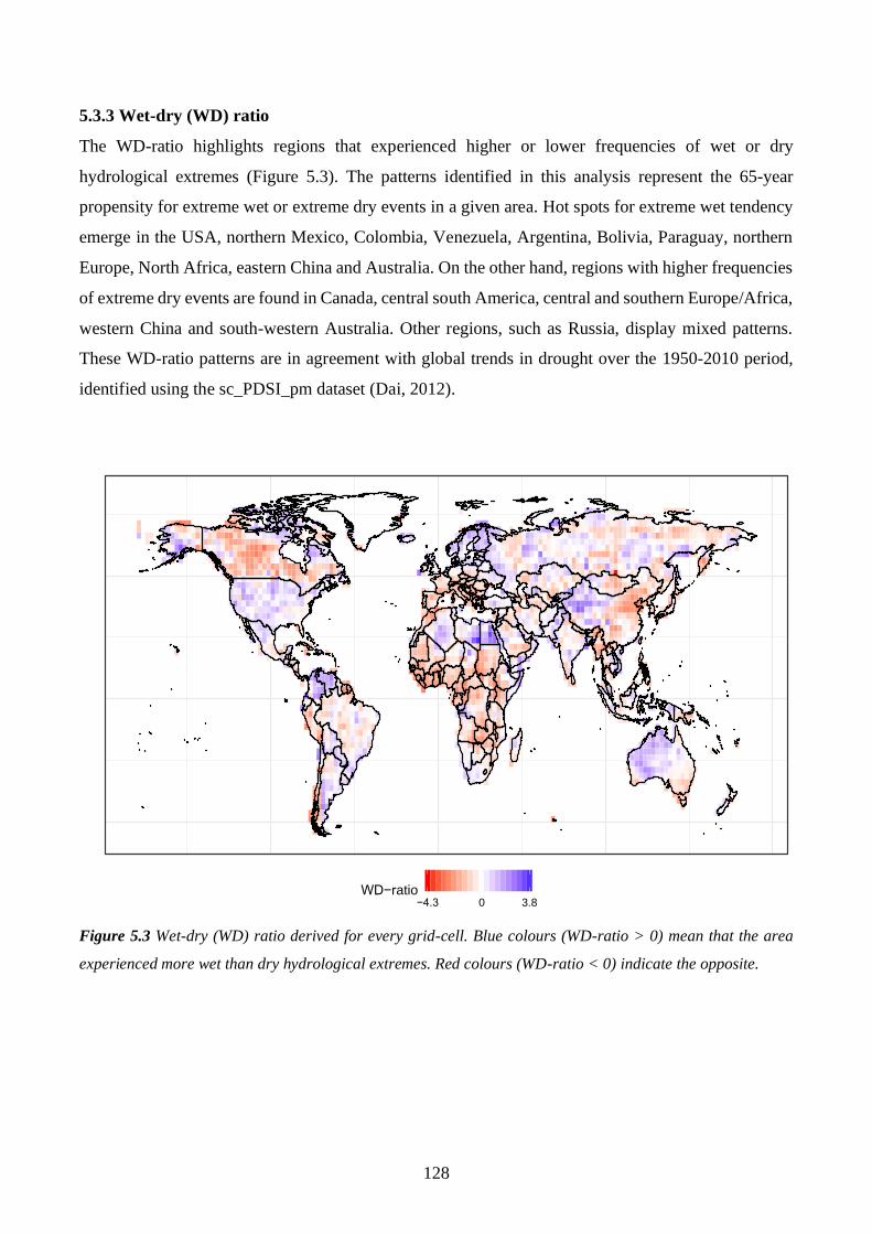
128

5.3.3 Wet-dry (WD) ratio

The WD-ratio highlights regions that experienced higher or lower frequencies of wet or dry

hydrological extremes (Figure 5.3). The patterns identified in this analysis represent the 65-year

propensity for extreme wet or extreme dry events in a given area. Hot spots for extreme wet tendency

emerge in the USA, northern Mexico, Colombia, Venezuela, Argentina, Bolivia, Paraguay, northern

Europe, North Africa, eastern China and Australia. On the other hand, regions with higher frequencies

of extreme dry events are found in Canada, central south America, central and southern Europe/Africa,

western China and south-western Australia. Other regions, such as Russia, display mixed patterns.

These WD-ratio patterns are in agreement with global trends in drought over the 1950-2010 period,

identified using the sc_PDSI_pm dataset (Dai, 2012).

Figure 5.3 Wet-dry (WD) ratio derived for every grid-cell. Blue colours (WD-ratio > 0) mean that the area

experienced more wet than dry hydrological extremes. Red colours (WD-ratio < 0) indicate the opposite.

−4.3 0 3.8WD−ratio

129

5.3.4 Extreme transitions (ET)

Figure 5.4a shows the extreme transitions (ET), in time interval (months), from wet to dry and dry to

wet extreme events within the period 1950-2014 plotted against the percentage of total land area

impacted. The ET from wet to dry (blue curve) exhibits a peak at 22-months with 4.3% of total land

having this mean time interval. On the other hand, ET from dry to wet (red curve) peaks at 18-month

with almost 5% of global land having this average separation time. Overall, ET from wet to dry takes

longer than ET from dry to wet. According to the boot-strap analysis, the ET for wet to dry extremes

are statistically significant in all grid-cells; for dry to wet only 10 grid-cells are not different from

chance. The cumulative distribution functions (CDFs) of wet to dry and dry to wet ET time intervals

are also shown (Figure 5.4b). For wet to dry 50% of the ET occur within ~27 months, whereas for dry

to wet 50% of ET are observed within 21 months. The two ET distributions are significantly different

(p-value <<0.01, Mann-Whitney-Wilcoxon test) under the null hypothesis that their means are equal.

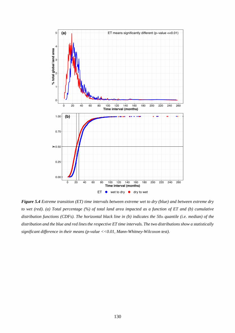
130

Figure 5.4 Extreme transition (ET) time intervals between extreme wet to dry (blue) and between extreme dry

to wet (red). (a) Total percentage (%) of total land area impacted as a function of ET and (b) cumulative

distribution functions (CDFs). The horizontal black line in (b) indicates the 50th quantile (i.e. median) of the

distribution and the blue and red lines the respective ET time intervals. The two distributions show a statistically

significant difference in their means (p-value <<0.01, Mann-Whitney-Wilcoxon test).

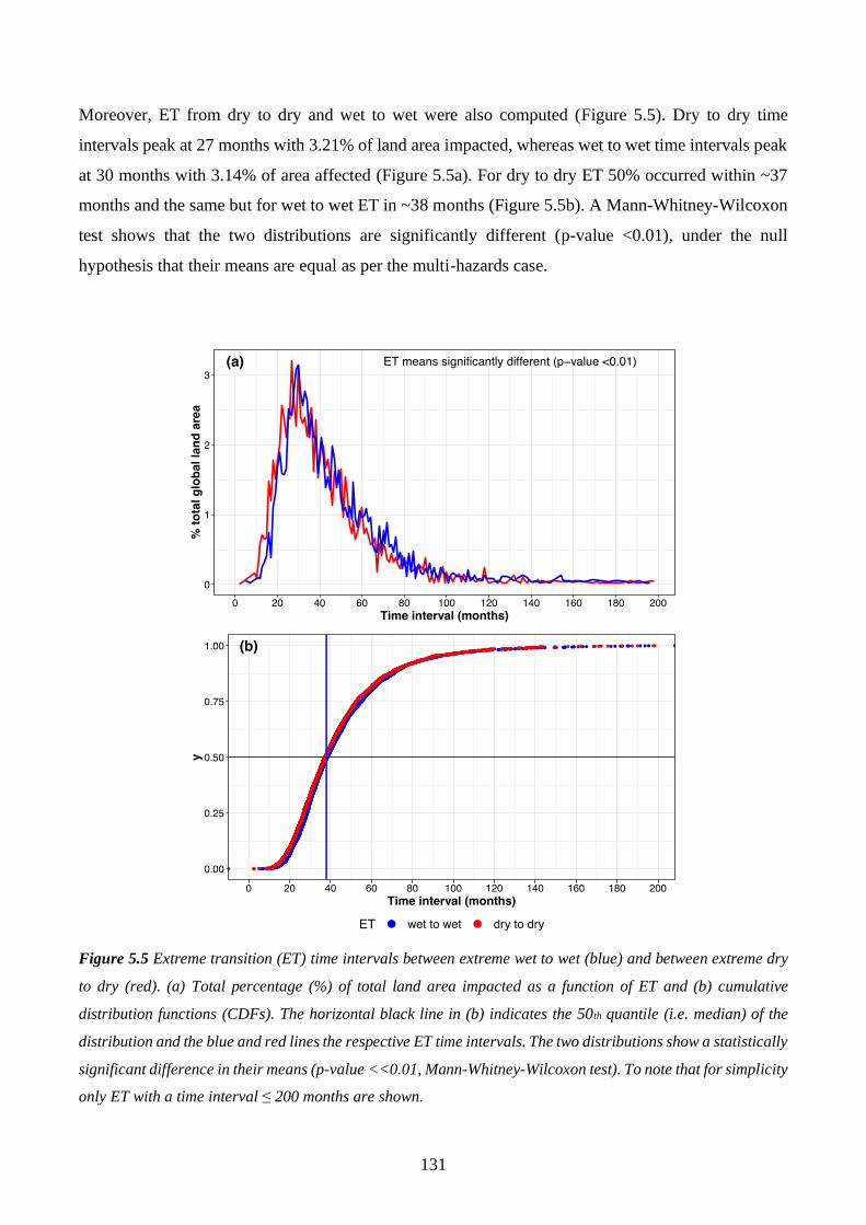
131

Moreover, ET from dry to dry and wet to wet were also computed (Figure 5.5). Dry to dry time

intervals peak at 27 months with 3.21% of land area impacted, whereas wet to wet time intervals peak

at 30 months with 3.14% of area affected (Figure 5.5a). For dry to dry ET 50% occurred within ~37

months and the same but for wet to wet ET in ~38 months (Figure 5.5b). A Mann-Whitney-Wilcoxon

test shows that the two distributions are significantly different (p-value <0.01), under the null

hypothesis that their means are equal as per the multi-hazards case.

Figure 5.5 Extreme transition (ET) time intervals between extreme wet to wet (blue) and between extreme dry

to dry (red). (a) Total percentage (%) of total land area impacted as a function of ET and (b) cumulative

distribution functions (CDFs). The horizontal black line in (b) indicates the 50th quantile (i.e. median) of the

distribution and the blue and red lines the respective ET time intervals. The two distributions show a statistically

significant difference in their means (p-value <<0.01, Mann-Whitney-Wilcoxon test). To note that for simplicity

only ET with a time interval ≤ 200 months are shown.

132

5.3.5 Correlations with climate indices

Figure 5.6 shows global correlations between hydrological extremes (wet and dry) and the three major

modes of climate variability (Niño3.4, PDO and AMO), which are known to have a significant effect

on regional precipitation/temperature patterns and hence flood and drought events. Details of the

calculation are provided in Section 5.2.4. The same correlation tests have been also computed for the

NAO (Barnston and Livezey, 1987), PNA (Barnston and Livezey, 1987) and QBO (Baldwin et al.,

2001), however the correlation coefficients were weaker compared to Figure 5.6 and very few of them

were statistically significant, as shown in Figure 5.7.

ENSO is one of the modes with the most widespread global impacts and in this study is represented

by the most widely used configuration, i.e. the Niño3.4 index (Figure 5.6a). The positive phase of

Niño3.4 (which can lead to El Niño events), is negatively correlated (p-value <0.05) with extreme wet

sc_PDSI_pm values over parts of central Canada, northern South America, southern Africa, India,

central China, central and northern Russia, Indonesia and eastern Australia. On the other hand, positive

and significant correlations are found over southern USA, in some scattered regions of central and

southern south-America and in the Middle East. This implies that a positive Niño3.4 phase is

associated with a lower likelihood of extreme wet hydrological events (sc_PDSI_pm ≥ 3) in these

regions, whereas negative Niño3.4 phase (possibly leading to La Niña events) typically enhances such

extremes.

In Figure 5.6b-c global partial correlations between hydrological extremes, measured with

sc_PDSI_pm, and PDO/AMO modes of climate variability with the ENSO signal removed are shown.

Correlations for PDO (Figure 5.6b) generally resemble the spatial patterns found for Niño3.4. In this

study, negative correlations are also found in north-western North-America, equatorial Africa and

eastern Russia. At the same time, almost all significant correlations over Australia, China and India

vanish. On the other hand, positive correlations are found in central-western USA, southern South-

America and Kazakhstan. The fact that Niño3.4 and PDO correlations show very similar spatial

patterns (Figures 5.6a-b) suggests that when these two indices are in phase (i.e. El Niño-warm PDO

and La Niña-cold PDO), wet and dry changes are magnified (Wang et al., 2014). The correlation

pattern shown in Figure 5.6b also agrees with season-ahead peak river flow correlations with the PDO

(Lee et al., 2018).

The pattern of AMO correlations (Figure 5.6c) differs from Niño3.4 and PDO indices and returns a

greater number of significant (p-value <0.05) grid-boxes than Niño3.4 (2.5% more grid-cells overall).

133

For the AMO, negative and significant correlations are found in Brazil, Argentina, Mexico, scattered

areas in north America, the Horn of Africa and eastern China. Positive correlations are found in the

Sahel region of Africa, Russia and central Asia. These results are again in agreement with global

season-ahead correlations found between peak river flows and AMO (Lee et al., 2018).

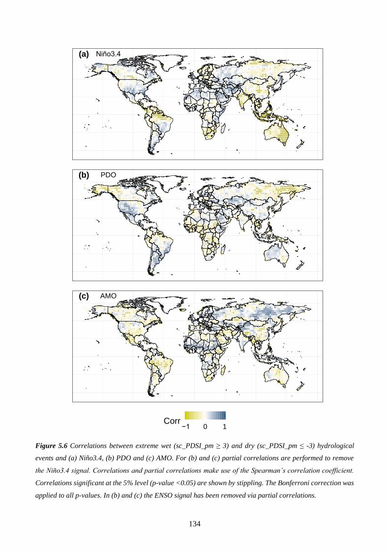
134

Figure 5.6 Correlations between extreme wet (sc_PDSI_pm ≥ 3) and dry (sc_PDSI_pm ≤ -3) hydrological

events and (a) Niño3.4, (b) PDO and (c) AMO. For (b) and (c) partial correlations are performed to remove

the Niño3.4 signal. Correlations and partial correlations make use of the Spearman’s correlation coefficient.

Correlations significant at the 5% level (p-value <0.05) are shown by stippling. The Bonferroni correction was

applied to all p-values. In (b) and (c) the ENSO signal has been removed via partial correlations.

●

●

●

●

●

●

●

●

●

●

●

●

●

●

●

●

●

●

●

●

●

●

●

●

●

●

●●●●

●

●

●

●

●

●

●

●

●

●

●

●

●

●

●

●

●

●

●

●

●

●

●

●

●

●

●

●

●

●

●

●

●

●

●

●

●

●

●

●

●

●

●

●

●

●

●

●

●

●

●

●

●

●

●

●

●

●

●

●

●

●

●

●

●

●

●

●

●

●

●

●

●

●

●

●

●

●

●

●

●

●

●

●

●

●

●

●

●

●

●

●

●

●

●

●

●

●

●

●

●

●

●

●

●

●

●

●

●

●

●

●

●

●

●

●

●

●

●

●

●

●

●

●

●

●

●

●

●

●

●

●

●

●

●

●

●

●

●

●

●

●

●

●

●

●

●

●

●

●

●

●

●

●

●

●

●

●

●

●

●

●

●

●

●

●

●

●

●

●

●

●

●

●

●

●

●

●

●

●

●

●

●

●

●

●

●

●

●

●

●

●

●

●

●

●

●

●

●

●

●

●

●

●

●

● ●

●

●

●

●

●

●

●

●

●

●

●

●

●

●

●

●

●

●

●

●

●

●

●

●

●

●

●

●

●

●

●

●

●

●

●

●

●

●

●

●

●

●

●

●

●

●

●

●

●

●

●

●

●

●

●

●

●

●

●

●

●

●

●

●

●

●

●

●

●

●

●

●

●

●

●

●

●

●

●

●

●

●

●

●

●

●

●

●

●

●

●

●

●

●

●

●

●

●

●

●

●

●

●

●

●

●

●

●

●

●

●

●

●

●

●

●

●

●

●

●

●

●

●

●

●

●

●

●

●

● ●

●

●

●

●

●

●

●

●

●

●

●

●

●

●

●

●

●

●

●

●

●

●

●

●

●

●

●

●

●

●

●

●

●

●

●

●

●

●

●

●

●

●

●

● ●

●

●

●

●

●

●

●

●

●

●

●

●

●

●

●

●

●

(a) Niño3.4

●

●

●

●

●

●

●

●

●

●

●

●

●

●

●

●

●

●

●

●

●

●

●

●

●

●

●

●

●

●

●

●

●

●

●

●

●

●

●

●

●

●

●

●

●

●

●

●

●

●

●

●

●

●

●

●

●

●

●●

●●●

●

●

●

●

●●●

●

●

●

●

●

●

●

●

●

●

●

●

●

●

●

●

●

●

●

●

●

●

●

●

●

●

●

●

●

●

●

●

●

●

●

●

●

●

●

●

●

●

●

●

●

●

●

●

●

●

●

●

●

●

●

●

●

●

●

●

●

●●

●

●

●

●

●

●

●

●

●

●

●

●

●

●

●

●

●

●

●

●

●

●

●

●

●

●

●

●

●

●

●

●

●

●

●

●

●

●

●

●

●

●

● ●

●

●

●

●

●

●

●

●

●

●

●

●

●

●

●

●

●

●

●

●

●

●

●

●

●

●

●

●

●

●

●

●

●

●

●

●

●

●

●

●

●

●

●

●

●

●

●

●

●

●

●

●

●

●

●

●

●

●

●

●

●

●

●

●

●

●

●

●

●

●

●

●

●

●

●

●

●

●

●

●

●

●

●

●

●

●

●

●

●

●

●

●

●

●

●

●

●

●

●

●

●

●

●

●

●

●

●

●

●

●

●

●

●

●

●

●

●

●

●

●

●

●

●

●

●

●

●

●

●

●

●

● ●

●

●

●

●

●

●

●

● ●

●

●

●

●

●

●

●

●

● ●

●

●

●

●

●

(b) PDO

●

●

●

●

●

●

●

●

●

●

●

●

●

●

●

●

●

●

●

●

●

●

●

●

●

●

●

●

●

●

●

●

●

●

●

●

●

●

●

●

●

●

●

●

●

●

●

●

●

●

●

●●●

●

●

●

●

●

●

●

●

●●

●

●●

●

●

●

●

●

●

●

●

●●

●

●

●

●

●

●

●

●

●

●

●

●

●

●

●

●

●

●

●

●

●

●

●

●

●

●

●

●

●

●

●

●

●

●

●

●

●

●

●

●

●

●

●

●

●

●

●

●

●

●

●

●

●

●

●

●

●

●

●

●●

●

●

●

●

●

●

●

●

●

●

●

●

●

●

●

●

●

●

●

●

●

●

●

●

●

●

●

●

●

●

●

●

●

●

●

●

●

●

●

●

●

●

●

●

●

●

●

●

●

●

●

●

●

●

●

●

●

●

●

●

●

●

●

●

●

●

●

●

●

●

●

●

●

●

●

●

●

●

●

●

●

●

●

●

●

●

●

●

●

●

●

●

●

●

●

●

●

●

●

●

●

●

●

●

●

●

●

●

●

●

●

●

●

●

●

●

●

●

●

●

●

●

●

●

●

●

●

●

●

●

●

●

●

●

●

●

●

●

●

●

● ● ●

●

●

●

●

●

●

●

●

●

●

●

●

●

●

●

●

●

●

●

●

●

●

●

●

●

●

●

●

●

●

●

●

●

●

●

●

●

●

●

●

●

●

●

●

●

●

●

●

●

●

●

●

●

●

●

●

●

●

●

●

●

●

●

●

●

●

●

●

●

●

●

●

●

●

●

●

●

●

●

●

●

●

●

●

●

●

●

●

●

●

●

●

●

●

●

●

●

●

●

●

●

●

●

●

●

●

●

●

●

●

●

●

●

●

●

●

●

●

●

●

●

●

●

●

●

●

●

●

●

●

●

●

●

●

●

●

●

●

●

●

●

●

●

●

●

●

●

●

●

●

●

●

●

●

●

●

●

●

●

●

●

●

●

●

●

●

●

●

●

●

●

●

●

●

●

●

●

●

●

●

●

●

●

●

●

●

●

●

●

●

●

●

●

●

●

●

●

●

●

●

●

●

●

●

●

●

●

●

●

●

●

●

●

●

●

●

●

(c) AMO

−1 0 1Corr

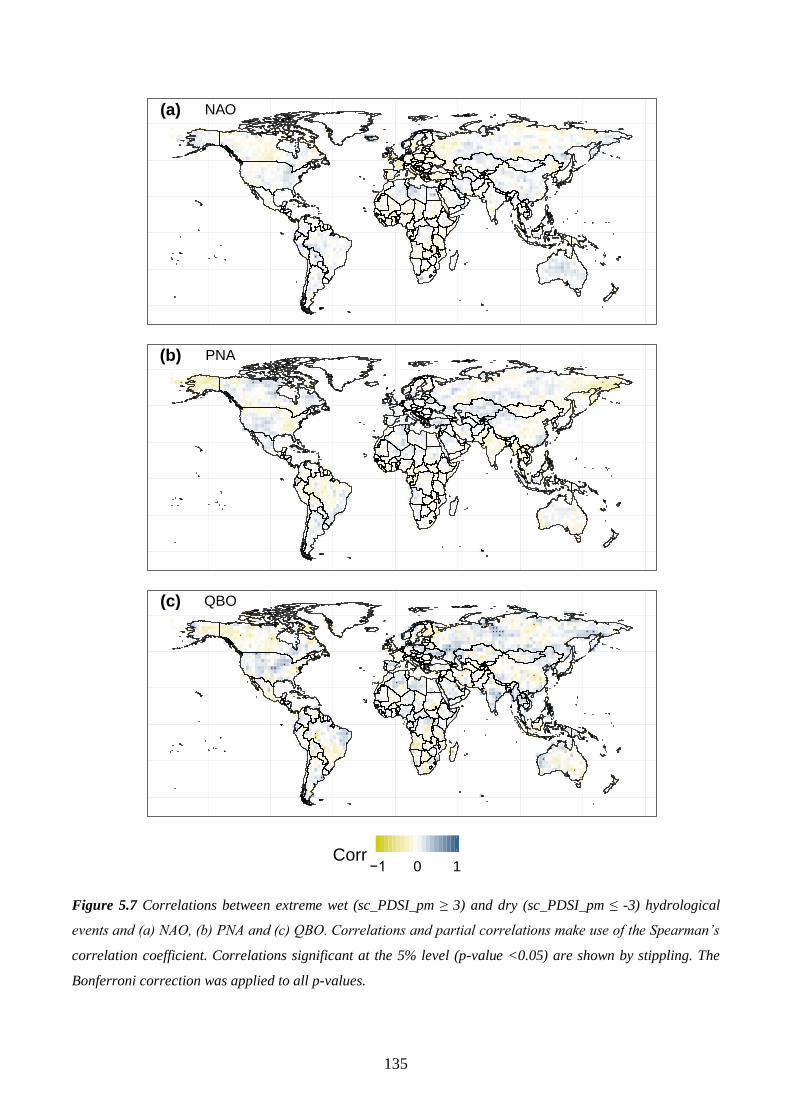
135

Figure 5.7 Correlations between extreme wet (sc_PDSI_pm ≥ 3) and dry (sc_PDSI_pm ≤ -3) hydrological

events and (a) NAO, (b) PNA and (c) QBO. Correlations and partial correlations make use of the Spearman’s

correlation coefficient. Correlations significant at the 5% level (p-value <0.05) are shown by stippling. The

Bonferroni correction was applied to all p-values.

●

●

●

●

●

●

●

(a) NAO

●●

● ●

●

●

(b) PNA

●

●

●

●

●

●

●

●

●

●

●

●

●

●

●

●

●

●

●●

●

●

●

●

●

● ●

●

●

●

●

●

●

●

●

●

●

●

●

●

●

●

●

●

●

●

●

●

●

●

●

● ●

(c) QBO

−1 0 1Corr

136

5.4 Discussion and Conclusions

Natural hazards, such as wet and dry extremes, can coincide over time and space creating multi-hazard

events in turn leading to significant socio-economic losses. Geographically remote co-occurring

extremes pose a potential economic risk to stakeholders with global assets and/or supply chains. For

instance, knowledge of recurrent patterns of coincident hydrological extremes could be used to hedge

losses, in regional hydropower production (Ng et al., 2017; Turner et al., 2017) and/or with respect to

crop yield (Leng and Hall, 2019; Xie et al., 2018; Zampieri et al., 2017), planting and harvesting (Sacks

et al., 2010). Relatively rapid successions of extremes at the same location pose challenges for disaster

preparedness, management and risk reduction. Thus, the maps shown in Figures 5.2 can therefore be

valuable for example for quantifying future concurrent wet-dry extreme events, within a global

seasonal forecasting product. Floods and droughts are expected to become more frequent and severe

in the future due to anthropogenic climate change (Arnell and Gosling, 2016; Dai, 2012; Hirabayashi

et al., 2013; IPCC, 2012), underscoring the importance of research on multi-hazard hydrological

extremes.

This chapter investigated a range of multi-hazard hydrological extremes at the global scale during the

period 1950 to 2014, with the primary objective of identifying the most geographically-widespread

events. The secondary goal was to develop new metrics for describing some of the properties of wet-

dry extremes, namely combinations of wet and dry extremes at locations, or their succession at a given

location. Answer to research question 1 is that the land area affected by extreme dry and geographically

remote wet-dry events has increasing and statistically significant trends. This coincides with the

expectation that such hazards are set to increase due to anthropogenic climate change (e.g. Güneralp

et al., 2015; Hirabayashi et al., 2013; IPCC, 2012), and is in agreement with previous studies (Dai,

2012, 2011b; Dai et al., 2004). In this chapter, however, a more stringent definition of extreme events

(De Luca et al., 2017), which captures well-known flooding and drought episodes has been applied. It

is further shown that these extremes can have global-scale impacts, by giving emphasis to the most

widespread wet, dry and wet-dry events. It is also found that the most widespread extreme wet and

wet-dry events occurred during December 2010 and the most extreme dry events during January 2003.

Such events provide an answer to research question 2 and they also coincided with well documented

floods and droughts occurring in remote regions across the globe.

Furthermore, research question 3 has been addressed by introducing two new metrics, the wet-dry

(WD) ratio and the extreme transition (ET) between wet/dry and dry/wet extremes. The former

137

discerns the local predominance of extreme wet or extreme dry events, by considering both types of

extremes simultaneously. Areas experiencing more wet than dry extremes were detected in the USA,

northern and southern South-America, northern Europe and North Africa, western China and most of

Australia. More dry than wet extremes were experienced in most of the remaining areas. Such

knowledge, if transferred into future projections, could raise awareness amongst emergency planners,

(re)insurance companies, farmers, relief organizations, and international agencies to better plan and

adapt to extreme wet and dry hydrological events. The ET metric estimates for every grid-cell the

average time interval between opposing extremes (i.e. transitions from wet to dry and from dry to wet).

The results show that the two ET time-series’ means differ significantly (p-value <<0.01) and that ET

between wet to dry are on average slower than dry to wet (22- versus 18-month interval on average).

Knowing long-term changes in ET time intervals between wet to dry and dry to wet hydrological

extremes can be significant for emergency planners, local businesses, governments and stakeholders.

For example, if average intervals shorten, losses could accrue more frequently, causing recurrent

shocks to local economies and, in some regions, impeding development.

The results obtained from the WD-ratio showed that some regions experienced more wet (dry) than

dry (wet) extremes in the past. In this chapter, the physical mechanisms driving such spatial patterns

were not explicitly investigated. However, since the sc_PDSI_pm dataset is computed by making use

of temperature and precipitation data, both dynamical and thermodynamic changes in the large-scale

atmospheric configuration (e.g. Harrington et al., 2019; Pfahl et al., 2017) can affect the spatio-

temporal patterns of sc_PDSI_pm wet and dry extremes. This implies for example that storm tracks,

blocking, localised convection, along with the increased water-holding capacity of the atmosphere due

to warmer temperatures (Trenberth, 2011) may have played a role in shaping the observed

predominance of wet and dry extremes. Similarly, mechanisms driving ET from wet (dry) to dry (wet)

were not addressed in this chapter. However, wet to dry ET happen on a slightly longer time-scale than

dry to wet ET, possibly implying that for the soil it is necessary more time to dry from a wet condition

than to become wet from dry. Such tentative explanation is similar to what can be driving a flash-

flood, i.e. heavy rainfall falling into dry soil with poor absorption ability (e.g. Collier, 2007; Doswell

et al., 1996).

The analysis in this chapter was based on the self-calibrated monthly-mean Palmer Drought Severity

Index, as it has been previously used in similar global studies (e.g. Dai, 2012, 2011b; Dai et al., 2004).

Future research opportunities include the use of other indices, such as the Standardized Precipitation

Index (McKee T.B., Doesken N.J., 1995; McKee et al., 1993) or the Standardized Precipitation

138

Evapotranspiration Index (Vicente-Serrano et al., 2010) to validate the findings and to account for

uncertainty in the observations of concurrent wet-dry extremes. Emphasis should also be given to

evaluating the seasonality of the extremes, since more robust and meaningful patterns could emerge,

specifically with respect to correlations with modes of climate variability. Similar analyses could be

applied to single Köppen climate zones (Rubel and Kottek, 2010) to discern possible regional

variations in concurrent wet-dry extreme characteristics. Finally, once baseline maps and data for

hydrological multi-hazards have been established from observations, the next step could be to

investigate with climate model output how these phenomena may change under anthropogenic climate

change.

To this end, and for providing an answer to research question 4, it is important to identify possible

climate drivers of the observed hydrological extremes. In this study, correlations between wet-dry

hydrological extremes and the corresponding values of the ENSO, PDO and AMO indices have been

computed. The global correlation patterns for ENSO confirm previous studies (Emerton et al., 2017;

Lee et al., 2018; Wang et al., 2014; Ward et al., 2014b), that investigated the effect of both El Niño

and La Niña events on global flood hazard and global season-ahead correlations between river peak

flows and climate indices, such as ENSO, PDO and AMO. It is worth highlighting that ENSO-induced

wet and dry changes are magnified when in phase with the PDO index. Global correlations are found

between the sc_PDSI_pm and PDO/AMO too. The PDO patterns generally match those of ENSO, and

this confirms the finding that when ENSO and PDO are in phase they amplify the global wet and dry

changes (Wang et al., 2014). The AMO, however, shows different and in some cases opposite

correlation patterns when compared to ENSO and PDO. Correlations of hydrological extremes with

modes of climate variability can be helpful for seasonal and sub-seasonal hydrological forecasting and,

in this case, they provide information about what kind of climate index phase is driving wet and dry

extremes in different regions globally. They also point to physical mechanisms, linked to climate

dynamics, which may have not been uncovered yet.

5.5 Summary

The research conducted in this Chapter focussed on a global analysis of observed concurrent wet and

dry hydrological extremes and their links with modes of climate variability (De Luca et al., 2019c).

The research made use of the self-calibrated monthly PDSI dataset based on the Penman-Monteith

model (Dai, 2017; Sheffield et al., 2012), along with the ENSO, PDO and AMO indices within the

139

1950-2014 period. Results showed that the land area impacted by dry and concurrent wet-dry

hydrological extremes increased significantly over the observational period. The most geographically

widespread wet, dry and concurrent wet-dry events were also identified and they match with well-

known flooding and drought episodes. Two new metrics were also introduced, namely the Wet-Dry

(WD) ratio and the extreme transitions (ET) between wet/dry and dry/wet extreme observations. The

former identifies the local predominance of extreme wet or extreme dry events. For example, areas

experiencing more wet than dry extremes were detected in the USA, northern and southern South-

America, northern Europe and North Africa, western China and most of Australia. Whereas the ET

estimates, for every grid-cell, the average time interval between opposing extremes. Results showed

that the two ET time-series’ (wet to dry and dry to wet) means differ significantly and that ET between

wet to dry are on average slower than dry to wet. Finally, global correlations between wet-dry

hydrological extremes and ENSO, PDO and AMO were also computed. Results to this end showed

marked similarity between ENSO and PDO spatial patterns, with different results obtained for AMO.

In conclusion, there is hope that these findings, in particular the maps shown in Figure 5.2-5.3, if

integrated for example into global forecasting products, may provide useful insights for disaster risk

reduction agencies, stakeholders and (re)insurance companies with assets spread worldwide, for

example in hydropower production (Ng et al., 2017; Turner et al., 2017) and/or crop yield (Leng and

Hall, 2019; Xie et al., 2018; Zampieri et al., 2017).

In the following Chapter 6 a discussion on the findings obtained from research Chapters 3-5 is

presented. Specifically, for each research chapter integrating themes focussed on multi-hazards will

be explored and further details on the application of the findings provided, along with links to the

wider literature.

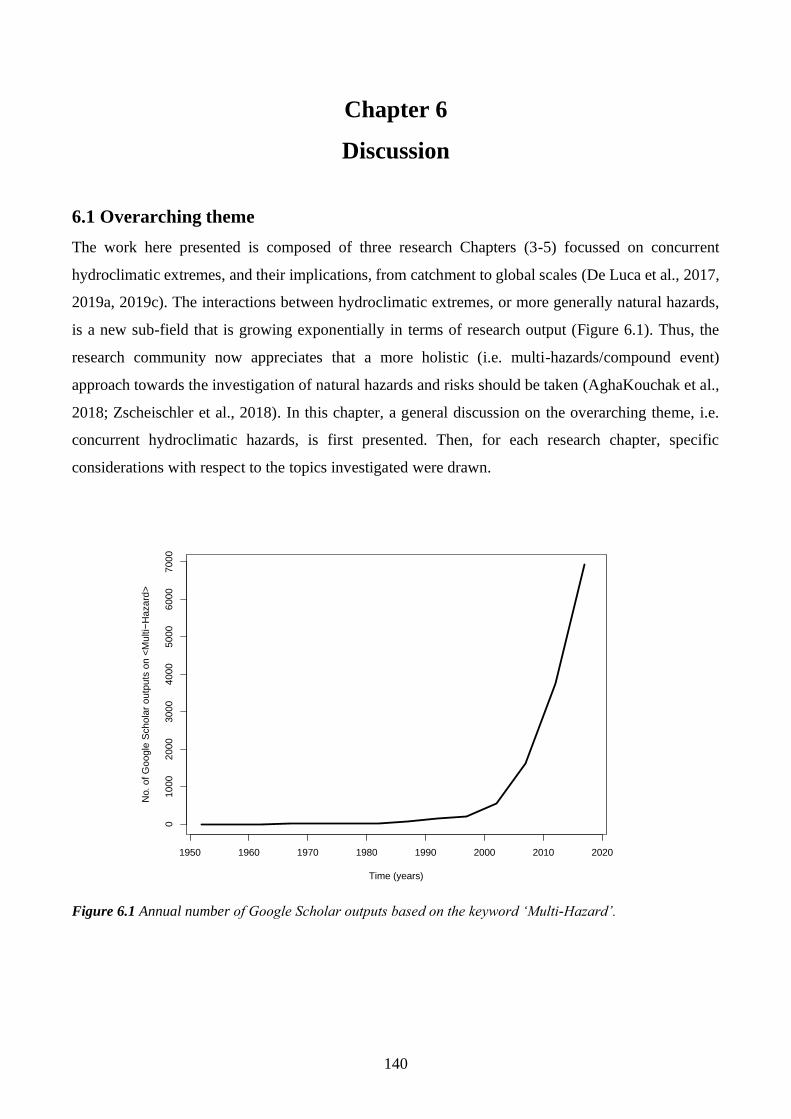
140

Chapter 6

Discussion

6.1 Overarching theme

The work here presented is composed of three research Chapters (3-5) focussed on concurrent

hydroclimatic extremes, and their implications, from catchment to global scales (De Luca et al., 2017,

2019a, 2019c). The interactions between hydroclimatic extremes, or more generally natural hazards,

is a new sub-field that is growing exponentially in terms of research output (Figure 6.1). Thus, the

research community now appreciates that a more holistic (i.e. multi-hazards/compound event)

approach towards the investigation of natural hazards and risks should be taken (AghaKouchak et al.,

2018; Zscheischler et al., 2018). In this chapter, a general discussion on the overarching theme, i.e.

concurrent hydroclimatic hazards, is first presented. Then, for each research chapter, specific

considerations with respect to the topics investigated were drawn.

Figure 6.1 Annual number of Google Scholar outputs based on the keyword ‘Multi-Hazard’.

1950 1960 1970 1980 1990 2000 2010 2020

010

00

20

00

30

00

40

00

5000

6000

7000

Multi−Hazards research growth

Time (years)

No. o

f G

oogle

Schola

r ou

tpu

ts o

n <

Multi−

Hazard

>

141

Natural hazards that can interact with each other and that are potentially affected by anthropogenic

climate change are currently attracting significant attention from the scientific community,

stakeholders, (re)insurance companies and emergency planners (e.g. Gill and Malamud, 2014; Kappes

et al., 2012a; Koks et al., 2019; Leonard et al., 2014; Munich Re, 2015; UNDRR, 2017a). This is

because their occurrence, strength and eventually socio-economic risks are set to likely increase in the

future mainly because of a warming climate (IPCC, 2018, 2012). For example, Gill and Malamud

(2014) provided a general overview of the relationships between 21 natural hazards, by identifying 90

different interactions and by emphasising the need of a multi-hazards approach towards natural hazard

assessments. Similarly, Kappes et al. (2012a) outlined the current challenges for a multi-hazard and

risk analysis, which are the choice of the approach (e.g. quantitative or semiquantitative), data and

method availability, scale issues and the awareness of limitations. Among international organisations,

the UN Sendai Framework for Disaster Risk Reduction (UNDRR, 2015) advocates a multi-hazard

approach. Case-studies investigating concurrent hydroclimatic hazards are numerous. For example,

national-scale analyses of flood and drought events in the UK (Collet et al., 2018; Visser-Quinn et al.,

2019), compound dynamical and observed extremes over Europe and Eastern North America (De Luca

et al., 2019b), global compound precipitation and wind extremes (Martius et al., 2016) and interactions

between river and coastal flooding (Ward et al., 2018). All these studies can help in enhancing disaster

risk reduction measures, by also bringing awareness of multi-hazards among the public and by

providing socio-economic benefits from local to global scales.

From an environmental science perspective, natural hazards cannot always be considered as

independent processes, because their occurrence, in time and space, is driven by physical variables

that may, in full or in part generate other, different perils. For example, excessive rainfall may lead to

flooding and trigger landslides, or tropical cyclones may generate both storm surges and fluvial

flooding, whilst also impacting the built environment with severe winds. Thus, much research effort

needs to be undertaken to assess the co-occurrence of these perils and not only because such events

stimulate an interest, but for providing robust insights that eventually will be used by international

organisations, governments and broadly-speaking stakeholders, to improve the socio-economic

resilience.

It is clear that the scientific community is currently investing resources and time to better disentangle

the common view of natural hazards as single processes (e.g. Gill and Malamud, 2014; Kappes et al.,

2012a; Leonard et al., 2014). This is excellent news. However, the circle is not closed yet, because

first of all there are still many research questions that need to be addressed (see for example Table 6.1)

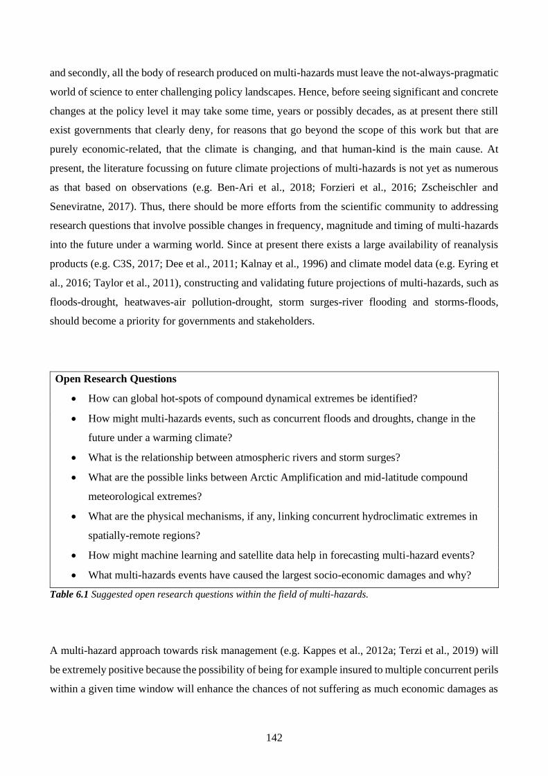
142

and secondly, all the body of research produced on multi-hazards must leave the not-always-pragmatic

world of science to enter challenging policy landscapes. Hence, before seeing significant and concrete

changes at the policy level it may take some time, years or possibly decades, as at present there still

exist governments that clearly deny, for reasons that go beyond the scope of this work but that are

purely economic-related, that the climate is changing, and that human-kind is the main cause. At

present, the literature focussing on future climate projections of multi-hazards is not yet as numerous

as that based on observations (e.g. Ben-Ari et al., 2018; Forzieri et al., 2016; Zscheischler and

Seneviratne, 2017). Thus, there should be more efforts from the scientific community to addressing

research questions that involve possible changes in frequency, magnitude and timing of multi-hazards

into the future under a warming world. Since at present there exists a large availability of reanalysis

products (e.g. C3S, 2017; Dee et al., 2011; Kalnay et al., 1996) and climate model data (e.g. Eyring et

al., 2016; Taylor et al., 2011), constructing and validating future projections of multi-hazards, such as

floods-drought, heatwaves-air pollution-drought, storm surges-river flooding and storms-floods,

should become a priority for governments and stakeholders.

Open Research Questions

• How can global hot-spots of compound dynamical extremes be identified?

• How might multi-hazards events, such as concurrent floods and droughts, change in the

future under a warming climate?

• What is the relationship between atmospheric rivers and storm surges?

• What are the possible links between Arctic Amplification and mid-latitude compound

meteorological extremes?

• What are the physical mechanisms, if any, linking concurrent hydroclimatic extremes in

spatially-remote regions?

• How might machine learning and satellite data help in forecasting multi-hazard events?

• What multi-hazards events have caused the largest socio-economic damages and why?

Table 6.1 Suggested open research questions within the field of multi-hazards.

A multi-hazard approach towards risk management (e.g. Kappes et al., 2012a; Terzi et al., 2019) will

be extremely positive because the possibility of being for example insured to multiple concurrent perils

within a given time window will enhance the chances of not suffering as much economic damages as

143

for the single-hazard case. Multi-hazards research has also a fundamental value in scientific

communication. Although local knowledge of a given territory plays an important role in managing

natural risks, the general public may not always be aware that the occurrence of a given hazard may

cascade or accumulate into a second or third peril. For example, a person could feel safe if he/she built

his/her house outside of a floodplain, however he/she may have not considered that the mountain above

the house is regularly subjected to landslides. In this case, heavy precipitation events, due to storms or

thunderstorms, lasting for a sufficient amount of time will eventually saturate the soil on the slopes of

the mountain and trigger landslides. Thus, local authorities have the duty to first gain knowledge,

through for example multi-hazard (risk) assessments, about possible combined perils affecting the area

and secondly, to inform residents about the risks via for example social media, scientific events,

newspapers and tv news. Furthermore, past extreme events could also be used as analogues for future

hazards (Matthews et al., 2016a).

6.2 Research contributions in context

With this thesis, several new insights on concurrent hydroclimatic hazards that can have significant

socio-economic impacts are highlighted.

In Chapter 3, interactions between observed multi-basin flooding and extra-tropical cyclones (ETCs)

in Great Britain (GB) are quantified and discussed (De Luca et al., 2017). First of all, a simple and

pragmatic method for identifying widespread flooding is presented and this, along with similar recent

studies (Berghuijs et al., 2019; Uhlemann et al., 2010), extends the conventional view of flooding that

is limited to a single river basin giving, for example, the opportunity to emergency managers to

estimate a national-scale return period of flooding. Secondly, multi-basin flooding in GB is found to

be linked with ETCs over a time-window of ~2 weeks. The research also used and introduced new

metrics, such as the F-Index (Wilby and Quinn, 2013), the (multi-basin) Flood-Yield and diverse

sources of data that captured different flood information. In the concurrent extremes scenario

introduced here, the risk of suffering socio-economic damage increases compared to a single hazard

case, because not only can a property be flooded, but the same structure may also be damaged by

severe winds. Such concurrent, widespread flood-wind impacts can therefore be also a cause of

significant stress to emergency services and insurance companies, if reasonable and adequate multi-

hazards prevention strategies are not deployed. For example, during a multi-basin flood coupled with

severe winds, more than one Environment Agency (EA) areas may be severely hit. Hence, the supply

144

chain for disaster relief needs to be able to provide enough support in diverse parts of the country,

through cross-collaboration and sharing of human and logistical resources.

In Chapter 4, an analysis of past and projected seasonal frequency and persistence of weather patterns

in the British Isles (BI) (Jenkinson and Collison, 1977; Jones et al., 1993; Lamb, 1972), along with

associated multi-hazards is presented (De Luca et al., 2019a). From the results obtained, one can

consider the future occurrence and related risks of two different cases of concurrent hydroclimatic

hazards. These are concurrent flood-wind events during winter and concurrent heatwave-air pollution

episodes in summer, with the latter focussed on London (UK). The weather patterns associated with

such multi-hazards scenarios are the cyclonic (C) and westerly (W) types for flood-wind impacts (e.g.

De Luca et al., 2017; Pattison and Lane, 2012) and the anticyclonic (A) type for heatwaves-air

pollution and drought events (e.g. Coumou et al., 2018; O’Hare and Wilby, 1995; Pope et al., 2015;

Wilby, 2008). Quantification of such concurrent hazards was achieved using two metrics, namely the

F-Score, an extension of the F-Index used in De Luca et al. (2017) and the nocturnal Urban Heat Island

(UHI) adapted from Wilby et al. (2011). Projected changes in the frequency and persistence of weather

patterns, along with their connected multi-hazards, can be indicative of future climate change impact

assessments and the methodology can be readily transferred to other mid-latitude regions and beyond

(e.g. Cortesi et al., 2013; Donat et al., 2010b; Grundström et al., 2015b; Lorenzo et al., 2008). Sensible

regions where the approach could be applied are for example the whole of Europe and its major cities,

where there is already concern about heat-air quality hazards (Bastin et al., 2019).

In Chapter 5, the research focussed on globally observed concurrent wet and dry hydrological extremes

and their association with modes of climate variability (De Luca et al., 2019c). Here, the most

geographically widespread and concurrent flood and drought episodes are quantified and presented as

maps. These findings provide new insights that are valuable for stakeholders and (re)insurance

companies with assets spread worldwide and invested for example in hydropower (Ng et al., 2017;

Turner et al., 2017) or crop (Leng and Hall, 2019; Xie et al., 2018; Zampieri et al., 2017) production.

They could also benefit road and railway infrastructures, as it is shown that globally about 27% of

these assets are exposed to at least one hazard, with billions of US $ contributing to global annual

expected damages (Koks et al., 2019). The proposed global maps could be, for example, integrated

into a seasonal/sub-seasonal hydrological forecasting model, so that information about multi-hazards

is made available to targeted businesses, emergency organisation and the wider public. Such new

development could be achieved by building an open-source online forecasting tool, updated for

example every 24h 7 days a week. On a similar line, multi-hazard hydrological forecasts could also

145

benefit from information about modes of climate variability, as there is a general consensus that

climate indices need to be incorporated, or used as predictors, within the models (Eden et al., 2015;

Emerton et al., 2019).

As per the previous two Chapters (3-4), the study also introduced two new metrics able to capture

information with respect to global wet and dry hydrological extreme observations, namely the Wet-

Dry (WD) ratio and the Extreme Transitions (ET). The former informs about whether there was a

predominance of extreme wet or extreme dry observations in the past, whereas the latter quantifies the

time-lag needed to pass from extreme wet (dry) to extreme dry (wet) conditions over a given area.

Overall, these results and metrics can also help emergency managers and governements, of

geographycally-large countries (e.g. USA, Russia and China), to better prepare and increase resilience

towards spatio-temporally concurrent flood and drought events. For example, future climate

projections of the WD-ratio up to 2100 could reveal the propensity of a given area to experience more

wet or dry extremes. Such information may be highly valuable, as stakeholders investing in irrigation

infrastructure or hydropower generation can adapt their long-term portfolio accordingly to the maps.

For example, if future WD-ratio projections show a region shifting from more dry to wet extremes,

farmers and stakeholders could consider investing infrastructures and crops’ resources in that area. On

the other hand, a projected shift from more wet to dry extremes can stop stakeholders from investing

in the given region. Similarly, future projections of the ET time-lag can benefit emergency managers

and broadly disaster risk reduction procedures, as knowing the time between for example a severe

flood and drought would be highly valuable for planning for example the disaster cycle phases (i.e.

response, recovery, mitigation and preparation).

6.3 Summary

This chapter provides a discussion of the overarching theme and contributions of each chapter, in a

wider context. Multi-hazards research has expanded considerably over the last decade, as the research

community realise that natural hazards can interact over time and space, and that their co-occurrence

may lead to more significant socio-economic damages than the single hazard components (Gill and

Malamud, 2014; Zscheischler et al., 2018). The multi-hazards subject also started to receive attention

from international organisations (UNDRR, 2017a) and there is hope that its importance will be also

soon be extended at the national, regional and local levels. However, for doing so, a significant shift

146

in legislations and regulations, expanding the common view of natural hazards to the possibility that

such events can develop into multi-hazards, must be made and if so, it will not be immediate.

A multi-hazards approach can be valuable for a different set of stakeholders and communities, such as

(re)insurance companies, emergency managers and environmental protection agencies. Concurrent

flood-wind hazards are somehow expected in GB, as the country is situated under the north Atlantic

storm-track. The results showed in Chapters 3-4 proved the existence of this association, along with

its enhanced occurrence in the future within a warmer world. Hence, such flood-wind scenario needs

to be considered by for example the government, EA and (re)insurance companies. The nocturnal UHI

temperatures for London and anticyclonic persistence and frequency in the BI (Chapter 4), during

summer, are also set to increase by the end of the 21st century. This could lead to an increased risk of

concurrent heatwave-air pollution-drought events, that can put under high stress the society and the

emergency management services. Lastly, in Chapter 5 the co-occurrence of wet and dry hydrological

extreme events is shown, along with documented impacts of the most geographically widespread ones.

These findings may help global stakeholders in hedging economic losses and governments of large

countries, that can experience both opposite extremes within the same time-frame.

In the next Chapter the conclusions will be drawn from each research chapter and overarching theme,

along with overall final remarks. Specifically, each chapter will be summarised, the research questions

revisited, future work directions presented, and the significance of the research highlighted. The

concluding remarks will focus on the hope for more urgent actions about anthropogenic climate

change, how this thesis fits into this landscape and how multi-hazards research can contribute with

respect to the climate issue.

147

Chapter 7

Conclusions

This thesis examined concurrent hydroclimatic hazards from catchment to global scales. Different

metrics were deployed for analysing the intereactions between hazards, with potential benefits for

stakeholders, policy makers and emergency managers. The topics investigated were combined

widespread flood-wind episodes (Chapter 3-4), future projections of weather pattern persistence and

associated multi-hazards (Chapter 4) and concurrent wet-dry hydrological extreme events (Chapter 5).

The time periods, covered observations spanning from 1950 to 2014, as well as climate model

historical runs for the observational period 1970-2000 and the future from 2011 to 2100. The

geographical domains under investigation were Great Britain (GB), the British Isles (BI) and the whole

globe. This chapter reprises the key literature gaps and related research questions, main findings of

this thesis, a discussion of the unifying theme and possible ways forward (Sections 7.1-7.3). Then, a

paragraph about the need for urgent actions about anthropogenic climate change can be found in

Section 7.4, before the very last Section 7.5 that draws out the general conclusion on the overarching

theme and how multi-hazards research could be integrated into anthropogenic climate change studies.

7.1 Concurrent flood-wind hazards

Chapter 3 reports the results of a multi-hazards study on observed extreme multi-basin flooding linked

with extra-tropical cyclones (ETCs) impacting GB (De Luca et al., 2017). The identified literature gap

was that river flooding if often investigated as a single-basin event, without considering the possibility

that within the same flooding episode, multiple basins can concurrently flood within a given window

of several days. At the time the research was started, only one study (Uhlemann et al., 2010) was found

addressing this research question. Chapter 3 advanced this work by adding a simple and pragamatic

methology, using annual maximum (AMAX) peak river flows, for extracting multi-basin flooding

events within a selected time-window of several days. Subsequently, Berghuijs et al. (2019) extended

the topic with a European assessment of synchronous flooding. However, the main literature gap was

that these widespread floods were not found to be associated with ETCs impacting GB, and that this

can eventually lead to a multi-hazards scenario of combined flood and wind socio-economic impacts.

148

The main research questions addressed in Chapter 3 were the following: i) What is the spatio-temporal

distribution of multi-basin flooding episodes? ii) What are the most frequent weather patterns observed

during these widespread floods? and iii) How are multi-basin floods, atmospheric rivers (ARs) and

very severe gales (VSGs) linked?

The results showed five extreme multi-basin flooding episodes within the 1975-2014 period and in a

time-window of 1 to 19 days. These matched with existing literature reporting widespread socio-

economic impacts across GB due to flooding. The peak flow annual maxima (AMAX), used as a proxy

for flooding, impacted between 66 to 108 basins and a total drained area (TDA) of 19% to 47% of the

study area during a window of 1 to 19 days. These events occurred during winter, with a frequency

peak in January and most common LWTs were the cyclonic (C) and westerly (W). Wet soil moisture

conditions, measured via the standardized precipitation index (SPI) (McKee et al., 1995; 1993)

preceded some of the episodes. Then it was also found that atmospheric rivers (ARs) (Brands et al.,

2016; Lavers et al., 2011) and VSGs (Jenkinson and Collison, 1977; Jones et al., 1993) occurred within

the same days or before the extreme multi-basin flooding episodes. Such findings, combining multi-

basin flooding with C-type weather patterns, ARs and VSGs established for the first time a compound

association between floods and ETCs (De Luca et al., 2017).

The methods and findings for extreme multi-basin flooding and ETCs have the scope to be extended

to other regions. Possible ways forward could be to upscale the domain of study to the whole of Europe,

USA or Canada as well as to conduct future hydroclimatic projections, for example through statistical

downscaling (Wilby and Wigley, 1997), under different Representative Concentration Pathways

(RCPs). Lastly, extreme value theory (EVT) (Coles, 2001) can provide insights into the statistical

coupling of both flooding and wind extreme values. This could be achieved by, for example, fitting a

multivariate extreme value model (e.g. Heffernan and Tawn, 2004), or simply by performing

correlation tests, between peak river flows and wind gust observations recorded in the same areas.

Specifically, one could select a network of river basins, covering a sufficiently large region (e.g. a

country or continent) and link each of these with wind gusts recorded from the closest meteorological

station.

Several benefits emerge from the research in Chapter 3. First, is the introduction of a new simple and

pragmatic method to quantify the temporal and spatial extent of multi-basin flooding episodes. Such

approaches can theoretically lead to the estimation of a national-scale return period of widespread

flooding, that will be useful to emergency managers and planners. This method is transferrable beyond

149

GB, although attention needs to be given to catchment area, as drainage networks within extremely

large basins may not necessarily be flooded entirely and within the same time-period as small

catchments. Second, it is found that multi-basin flooding events can cause socio-economic damages

that in some cases go beyond what is planned for by emergency agencies and affect local communities

and businesses (De Luca et al., 2017). Third, such damages can be amplified by coupled severe wind

impacts. The results expose a compound risk that needs to be covered by (re)insurance companies,

emergency managers and stakeholders.

7.2 Weather pattern persistence and multi-hazards

Chapter 4 investigated observed and future seasonal climate projections of Lamb Weather Types

(LWTs) (Jenkinson and Collison, 1977; Jones et al., 1993; Lamb, 1972) frequency and persistence

within the BI and their links with multi-hazards (De Luca et al., 2019a). The main literature gap was

the lack of studies linking weather patterns to multi-hazards, such as flood-wind and heatwave-air

pollution-drought events. Moreover, no previous research has brought this topic into light by

performing climate model evaluation and projections up to 2100.

The specific research questions addressed by Chapter 4 were the following: i) How has persistence in

weather pattens changed historically? ii) To what extent can Atmosphere-Ocean General Circulation

Models (AOGCMs) reproduce observed weather pattern persistence over the BI? iii) How are weather

pattern persistence and frequency expected to change in the future under different Representative

Concentration Pathways (RCPs)? and iv) How migth variations in future weather type persistence

translate into changed risk of winter flood-wind and summer heatwave-air pollution concurrent

hazards?

The results showed that AOGCMs are generally capable of reproducing weather pattern seasonal

persistence when compared with NCEP (Kalnay et al., 1996) and 20CR (Compo et al., 2011)

reanalyses products, across the historical 1971-2000 (1980s) period. Persistence for the anticyclonic

(A) type is projected to increase in the future during summer; cyclonic (C) weather on the other hand

decreases in all seasons and the westerly (W) type does not change in winter, but increases in autumn

and decreases in spring under RCP8.5. Moreover, the frequencies of A- and W-types are projected to

increase significantly by 2100 during summer and winter respectively (RCP8.5, p-value <0.01).

Whereas C-type frequency during autumn is projected to decrease during autumn (p-value <0.01).

150

With respect to multi-hazards, two metrics, the F-Score and the nocturnal Urban Heat Island (UHI)

temperatures, were computed respectively for concurrent winter flood-wind and summer heatwave-air

pollution events. Results showed that the F-Score is overestimated by the AOGCMs when compared

to NCEP, 20CR reanalyses and Lamb’s subjective dataset. However the risk of concurrent flood-wind

events is set to significantly increase by 2100. On the other hand, the nocturnal UHI temperatures for

London (UK) are slightly underestimated by AOGCMs, and as per the F-Score, severity is projected

to significantly increase by 2100.

Further possible research on the topic could be undertaken by applying the same persistence and

frequency method to other regions with established weather pattern typologies, such as the

Grosswetterlagen for Europe (Hess and Brezowsky, 1952) and Spatial Synoptic Classification for

North America (Kalkstein et al., 1996). The analysis could also be extended by making use of a larger

ensemble of both reanalyses and AOGCMs, and by investigating other types of multi-hazards

scenarios, such as concurrent river flooding-storm surges and/or flood-drought events.

The findings for the A-type weather pattern may signify an increased chance of blocking episodes

which could increase the risk of poor air quality, droughts and heatwaves during summer (Coumou et

al., 2018; Munich Re, 2015; Tang et al., 2013). These changes could be linked to Arctic Amplification

(AA) (Screen and Simmonds, 2010) but are difficult to reconcile with a projected decrease in blocking

events over the BI during summer by 2061-2099 under RCP8.5 (Woollings et al., 2018). A decrease

in persistence and frequency for the C-type during autumn can imply reduced chance of extreme

precipitation and flooding, linked to ETCs impacting the BI (De Luca et al., 2017); whereas a more

frequent W-type (or zonal flow) during winter can bring high rainfall events and possible fluvial

flooding (Pattison and Lane, 2012). Results for multi-hazards suggest that by the end of the 21st

century, there could be an increasing chance of concurrent flood-wind hazards during winter and

concurrent heatwave-air pollution hazards during summer (in London). These findings bring new

insights into future projections of concurrent climate extremes in the BI. They can be valuable for

governments when it comes to increasing resilience against concurrent hydroclimatic extremes.

Finally, the methodology can help in both evaluating AOGCMs realism as well as providing narratives

of future hydroclimatic risks that can be intelligible to a wide range of user communities.

151

7.3 Concurrent wet and dry hydrological extremes

Chapter 5 examined concurrent wet and dry hydrological extremes at the global scale and their

relationship with modes of climate variability (De Luca et al., 2019c). The literature gaps filled by the

chapter were (a) the lack of a global observational analysis of spatio-temporal joint occurrences of

extreme wet and dry events, (b) metrics to investigate such opposed extremes and (c) studies showing

how these extremes are linked with predominant climate indices.

The research questions were the following: i) How have observed globally independent and concurrent

wet-dry hydrological extreme events changed in the past? ii) What were the most spatially extensive

independent and concurrent wet-dry hydrological extreme events? iii) How might new metrics shed

light into the likelihood of concurrent wet-dry extremes? and iv) How are these extremes related to

different modes of climate variability?

The results presented in Chapter 5 contribute to a deeper understanding of concurrent wet and dry

hydrological extremes. First, it is shown that the global land area impacted by dry and wet-dry extreme

events significantly increased during the period 1950-2014. The most geographically widespread wet,

dry and wet-dry events coincided with well known flooding and drought episodes around the globe.

Second, the two metrics developed (namely the Wet-Dry, WD ratio and the Extreme Transitions, ET)

provided insights into the past predominance of wet or dry extremes in a given area and about the

globally aggregated time-lag between a wet (dry) and dry (wet) extreme observation respectively. The

WD-ratio identified regions that experience more wet than dry extremes as the USA, northern and

southern South-America, northern Europe, North Africa, western China and most of Australia. The

remaining regions, on the other hand, show a predominance of dry extremes. Third, the ET between

wet to dry are on average significantly slower than the ones from dry to wet. Finally, global correlations

between climate indices and wet and dry extremes showed that the El Niño Southern Oscillation

(ENSO) and Pacific Decadal Oscillation (PDO) have patterns of positive correlations with wet

extremes over southern and western USA, south Brazil and Argentina and the middle-east. Conversely,

significant negative correlations were found over north-western North America, northern Brazil,

central and southern Africa, eastern Russia, Indonesia and eastern Australia. On the other hand, the

Atlantic Multidecadal Oscillation (AMO) generally exhibited opposite correlation patterns when

compared to ENSO and PDO.

152

These analyses could be extended in different ways, so that a more profound understanding of the joint

spatio-temporal occurrences of global wet and dry extremes, can be achieved. For example, Chapter 5

made use of the self-calibrated Palmer Drought Severity Index based on the Penman-Monteith model

(sc_PDSI_pm) (Dai, 2017; Sheffield et al., 2012). Thus, there is scope for replicating the work by

using other global hydrological datasets such as the Standardized Precipitation Index (SPI) (McKee

T.B., Doesken N.J., 1995; McKee et al., 1993) or the Standardized Precipitation Evapotranspiration

Index (Vicente-Serrano et al., 2010). This would also reveal the sensitivity of the present findings to

the choice of hydrological data. Moreover, analysing concurrent seasonal wet and dry extremes may

also be relevant, as stronger spatio-temporal patterns may emerge when compared to the annual time-

scale. The wet-dry extremes could also be differentiated by Köppen climate zones (Rubel and Kottek,

2010), so that their variations can be objectively assigned to specific regions of the world. Lastly, once

solid observational results are established, the next step would be to perform AOGCMs simulations

and project future changes of concurrent wet and dry hydrological extremes for a warming world.

The findings in Chapter 5, on the spatio-temporal co-occurrence of wet and dry hydrological extremes,

are relevant to stakeholders with global assets and/or supply chain. Thus, understanding the behaviour

of future concurrent wet and dry extremes, through maps of the most widespread events and future

projections of the WD-ratio, can help for example in hedging economic losses with respect to regional

hydropower production (Ng et al., 2017; Turner et al., 2017), crop yields (Leng and Hall, 2019; Xie et

al., 2018; Zampieri et al., 2017), planting and harvesting schedules (Sacks et al., 2010), and global

transport networks (Koks et al., 2019). Furthermore, future projections of the ET would be useful for

improving disaster risk reduction measures, through an enhancement of resilience.

7.4 The climate is already changing, what about us?

It is apparent that citizens and governments are becoming more aware of the greatest problem human-

kind is currently facing, i.e. anthropogenic climate change and its related socio-economic impacts due

to weather and climate extremes (IPCC, 2018, 2012; UNDRR, 2015). As a consequence, many

countries, such as Sweden, Iceland, Norway and Ireland are investing heavily in renewable energy

resources. Thus, there is great hope among these leading countries that the socio-economic impacts of

climate change can be significantly mitigated, so that future generations will be able to continue living

a decent and sustainable life. Many things however, still need to change, as at present there is still a

lack of general consensus among all the governements about the fact that the climate is changing and

153

that we, as human-kind, are the main cause of the issue. Such a thing is something that needs to be

addressed and fixed as soon as possible, because at the moment some of the countries denying climate

change (e.g. USA, Brazil, Russia and Saudi Arabia) are among the largest greenhouse gas producers.

The world at present really needs top-down and bottom-up political actions against climate change and

its influence on weather and climate extremes, so that fossil fuels will be replaced with renewable

energies, significant investment in research tackling extreme events will be made, sustainable

adaptation measures will be deployed and a green and sustainable economy will be incentivised. It is

also clear that leaders who refuse or delay to act against climate change are not doing so because they

do not realise the gravity of the issue, or because they are wrongly advised by the scientific community,

but simply because short-term economic interests do not allow tackling climate change. It is also true

that if each person in the world does a little to reduce his/her carbon footprint the advantage for us can

be enormous (e.g. mantaining a vegetarian diet, reducing the electric consumption at home, buying

electric cars, etc..). However, the truth is that the greatest changes towards a greener planet need to

come from governments and politicians, as they are the only ones heard by the people.

Thus, a possible way forward, which at the moment is definitely growing with importance and taking

place around the world, is to educate and sensitise the old but in particular the young generations about

the fact that: i) climate change is currently happening; ii) climate change is having a significant effect

on exacerbating the magnitude and frequency of weather and climate extremes, with even more

devastating socio-economic impacts; iii) if actions are not taken in full, the outcomes may lead to

irreparable damages to human-kind; and iv) that solutions to tackle the problem currently exist, but

they can only materialise with targeted political choices and actions. The climate on earth has always

changed and it will continue to do so with or without our presence. Human-kind represents only a tiny

and possibly insignificant temporal breath over the entire earth’s life. The earth will definitely survive

this current anthropogenic climate change, but will we survive stronger and more frequent weather

and climate extremes? It is therefore in the best interest of all people on earth to accept the scientific

consensus about climate change and to urge for more actions, not because we will be able to see any

positive difference in our lifetime, but because we will be able to donate to future generations a world

that is still able to provide a livable environment.

154

7.5 Concluding remarks about multi-hazards

There is hope that this thesis on concurrent hydroclimatic hazards highlights the importance of

continuing investment of time and resources into research focussed on the understanding of concurrent

weather, climate and hydrological hazards and risks. More research is indeed required in this field and

it also needs to be translated by policy makers and stakeholders, into concrete solutions and actions

that can eventually enhance socio-economic resilience to extreme events at the global, regional,

national and local scales. In particular, since a new sub-field of research focussing on multi-hazards,

or compound events, (e.g. Gill and Malamud, 2014; Zscheischler et al., 2018) has been now

established, new research questions arise along with the need to put into practice the findings coming

from the research community. Natural hazards that are driven by the atmosphere (e.g. floods, droughts,

heatwaves and storms) are likely to become more severe in the future due to anthropogenic climate

change (IPCC, 2018, 2012). This statement is just one of the many highlighting the immediate need

of pragmatic solutions to better prevent, adapt to and better predict concurrent weather, climate and

hydrological hazards and associated impacts.

At present, despite a growing body of literature reviewing multi-hazards (e.g. Gill and Malamud, 2017,

2014; Kappes et al., 2012b, 2012a; Leonard et al., 2014; Terzi et al., 2019; Tilloy et al., 2019;

Zscheischler et al., 2018) and numerous studies investigating diverse interrelationships between the

perils (e.g. Collet et al., 2018; De Luca et al., 2019b; Koks et al., 2019; Martius et al., 2016; Visser-

Quinn et al., 2019; Ward et al., 2018), very little has been done with respect to future climate

projections of compound events (Ben-Ari et al., 2018; Forzieri et al., 2016; Zscheischler and

Seneviratne, 2017). Thus, a general way forward within the field of multi-hazards would be indeed to

build international projects, between research institutes, universities, companies and policy makers,

focussed on future scenarios of multi-hazard events under a warming world.

Such research, could focus on hazard interactions including: i) future projections and links to the Arctic

Amplification (Screen and Simmonds, 2010); ii) global assessments of future socio-economic damages

from multi-hazards; iii) the discovery of new physical multi-hazard processes (e.g. atmospheric rivers

driving storm surges and river flooding); iv) spatio-temporal shifts in the distribution of multi-hazards

and v) the application of multivariate extreme value statistics (e.g. Heffernan and Tawn, 2004) and

dynamical systems theory (De Luca et al., 2019b; Faranda et al., 2017b, 2017a; Hochman et al., 2019;

Lucarini et al., 2016, 2012; Messori et al., 2017; Rodrigues et al., 2018) to climate projections (Faranda

et al., 2019). Such research efforts could also focus on different spatial scales, from cities, to countries,

155

continents and global areas. They should also involve multi-disciplinary teams, spanning the social

sciences, philosophy, mathematics, physics, computer science, geography and engineering.

In conclusion, this thesis analysed different sets of concurrent hydroclimatic hazards, from catchment

to global scales using both observations and climate model projections. It is shown that in Great Britain

extreme multi-basin flooding is linked to extra-tropical cyclones. The work also reveals that concurrent

flood-wind and heatwave-air pollution-drought hazards could increase in the future, and that

substantial areas of the world can be impacted by concurrent yet geographically-remote flood and

drought events. This matters because, apart the fact that such multi-hazard events are extremely

fascinating per se, they can generate enormous socio-economic damages, which should be understood

and managed.

156

Annex 1

A.1 Supplementary Information Chapter 3

A.1.1 Figures

Figure S3.1 Initial hydrological network of 649 gauges. The yellow stations are the 261 non-nested basins used

in the analyses, whereas blue stations represent the remaining 388 nested stations excluded from the study

because they are located upstream from a non-nested gauge.

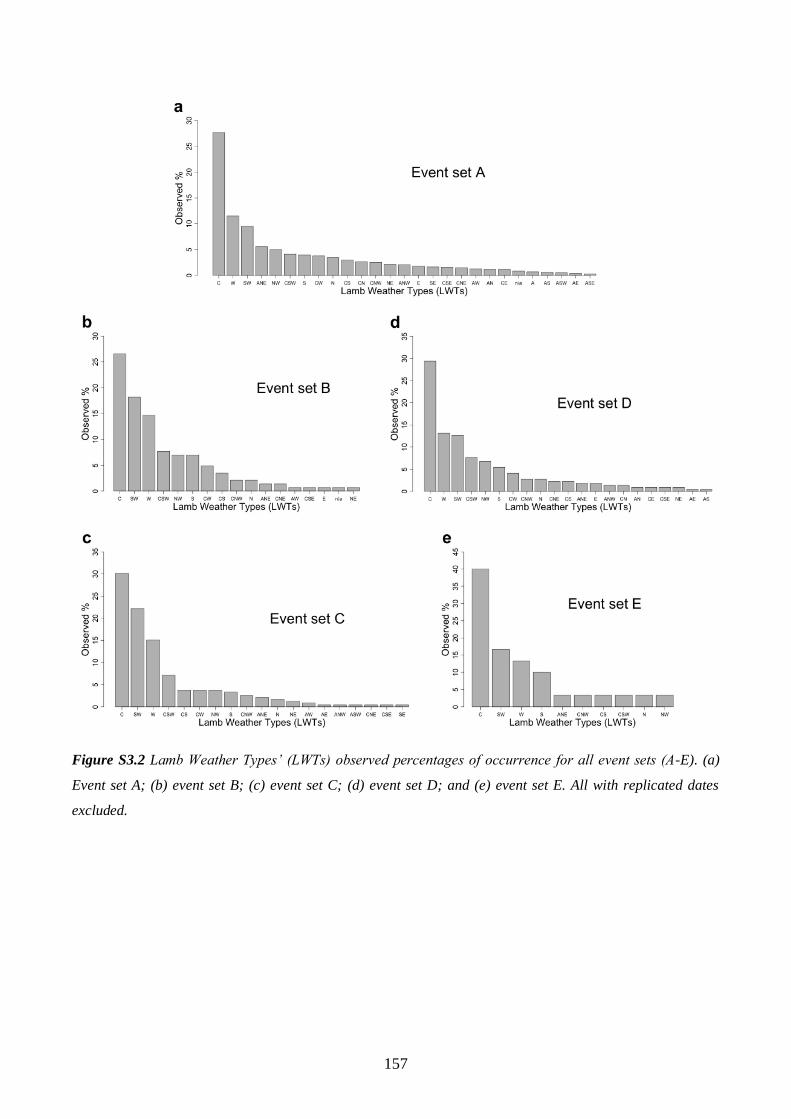
157

Figure S3.2 Lamb Weather Types’ (LWTs) observed percentages of occurrence for all event sets (A-E). (a)

Event set A; (b) event set B; (c) event set C; (d) event set D; and (e) event set E. All with replicated dates

excluded.

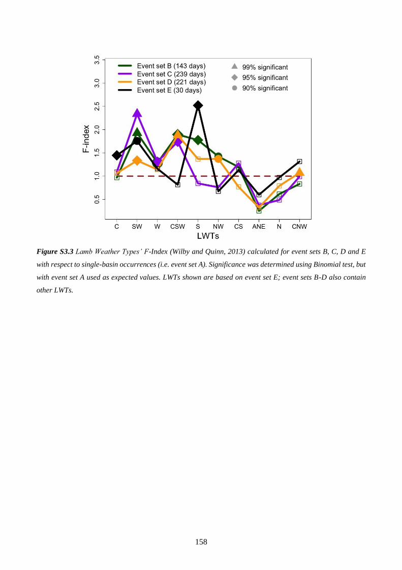
158

Figure S3.3 Lamb Weather Types’ F-Index (Wilby and Quinn, 2013) calculated for event sets B, C, D and E

with respect to single-basin occurrences (i.e. event set A). Significance was determined using Binomial test, but

with event set A used as expected values. LWTs shown are based on event set E; event sets B-D also contain

other LWTs.

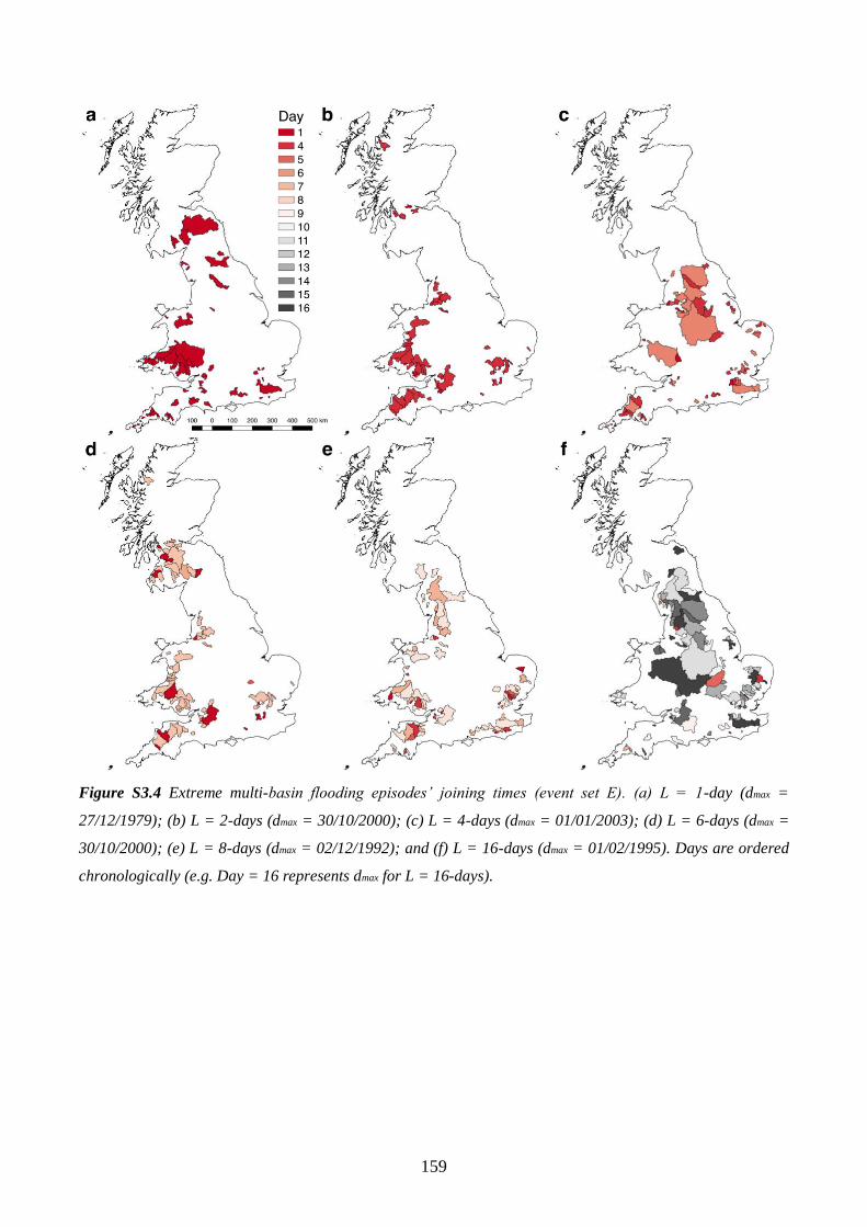
159

Figure S3.4 Extreme multi-basin flooding episodes’ joining times (event set E). (a) L = 1-day (dmax =

27/12/1979); (b) L = 2-days (dmax = 30/10/2000); (c) L = 4-days (dmax = 01/01/2003); (d) L = 6-days (dmax =

30/10/2000); (e) L = 8-days (dmax = 02/12/1992); and (f) L = 16-days (dmax = 01/02/1995). Days are ordered

chronologically (e.g. Day = 16 represents dmax for L = 16-days).

160

Annex 2

A.2 Supplementary Information Chapter 4

A.2.1 Methods

A.2.1.1 CMIP5, reanalyses and Lamb’s catalogue

The climate model output used to represent historical, future Representative Concentration Pathway

8.5 (RCP8.5) and RCP4.5 projections of LWTs (Jones et al., 1993; Lamb, 1972) originate from a

multi-model sub-ensemble (MME) of 10 Atmosphere-Ocean General Circulation Models (AOGCMs)

from the Coupled Model Intercomparison Project Phase 5 (CMIP5) (Taylor et al., 2011). MME output

was obtained from the Earth System Grid Federation (https://esgf-node.llnl.gov/search/cmip5/). Per

each model the historical, RCP8.5 and RCP4.5 runs of daily (12 UTC) sea-level pressure (SLP) are

used to calculate daily LWTs across the BI as described above. The historical period is defined as

1980s (1971-2000). Model runs for the RCPs (2006-2100) are divided into consecutive 30-year periods

covering the 2020s (2011-2040), 2050s (2041-2070) and 2080s (2071-2100). Each AOGCM was re-

gridded to 5°×10° (latitude × longitude) to match the grid of the objective LWT classification

(Jenkinson and Collison, 1977; Jones et al., 1993). The choice of AOGCMs was constrained by

availability of daily SLP for historical, RCP8.5 and RCP4.5 runs. Table 4.1 lists these models along

with some of their characteristics.

To evaluate CMIP5 MME realism, LWTs were derived from two reanalyses (Jones et al., 2013) then

compared with the 30-year historical (1980s) run of the MME. These were the 20CR (Compo et al.,

2011) and NCEP (Kalnay et al., 1996) LWTs datasets (Jones et al., 2013), available from

https://crudata.uea.ac.uk/cru/data/lwt/. In addition to reanalyses, a comparison of the historical MME

with Lamb’s catalogue of subjectively defined LWTs (Hulme and Barrow, 1997; Lamb, 1972), which

ends in 1997, is also provided. The MME realism is evaluated using LWTs occurring in four seasons,

namely: summer (June-July-August, JJA); autumn (September-October-November, SON); winter

(December-January-February, DJF); and spring (March-April-May, MAM). Seasons were assigned to

the year with the first month (e.g. summer 2020 includes June 2020, July 2020 and August 2020, whilst

winter 2000 includes December 2000, January 2001 and February 2001). Note that for Lamb’s

catalogue, DJF for the 1980s has December and January for winter 1996, because the dataset ends in

early February 1997. All the complete LWTs datasets used in the analyses are provided in the csv files

accompanying this study.

https://esgf-node.llnl.gov/search/cmip5/

https://crudata.uea.ac.uk/cru/data/lwt/

161

A.2.1.2 Statistical methods and analyses

A.2.1.2.1 2-day persistence

2-day persistence of LWTs (Jones et al., 1993; Lamb, 1972) was derived from Markov-chain matrices

of transitions between the eight main weather types defined above (Gagniuc, 2017; Wilby, 1994).

Persistence was defined as the probability that a given LWT on day(t) is followed by the same LWT

on day(t+1). LWTs persistence is calculated for each AOGCM and MME mean (MMEM) for

historical 1980s and 2020s, 2050s, 2080s under RCP8.5 and RCP4.5. Uncertainty in persistence

estimates for the CMIP5 MME 1980s was calculated by boot-strapping (n=1,000) 30-year simulations

to obtain 95% confidence intervals for significance testing. Persistence for the 2020s, 2050s and 2080s

was calculated from the transition matrices. Persistence analysis was performed using the functions

markovchainFit and createSequenceMatrix, from the R package ‘markovchain’ (Spedicato, 2017),

respectively for historical boot-strapping and the three future periods (https://cran.r-

project.org/web/packages/markovchain/markovchain.pdf). To evaluate the performance of the CMIP5

MME, the 20CR (Compo et al., 2011), NCEP (Kalnay et al., 1996), and Lamb’s subjective

classification (Hulme and Barrow, 1997; Lamb, 1972) were also used to calculate LWT persistence

during the 1980s period. The CMIP5 MME historical persistence for 1971-1996 (not shown here) is

also computed, to test the slightly shorter period covered by Lamb’s subjective catalogue. After

performing a Mann-Whitney-Wilcoxon two-tailed test (Mann and Whitney, 1947) (null hypothesis of

no difference in mean persistence), between the MME 1971-1996 and MME 1980s, for A, C, W, and

S LWTs within respectively summer (JJA), autumn (SON), winter (DJF) and spring (MAM), it is

found no statistical significance between the two periods. Therefore, it is possible to conclude that

Lamb’s catalogue is equivalent to the 1980s, despite being 5 years shorter.

The seasonal persistence for each LWT, AOGCM, MMEM, 20CR, NCEP and Lamb’s subjective

catalogue during the 1980s and (for AOGCMs only) 2020s, 2050s and 2080s under RCP8.5 and

RCP4.5 are provided in the spreadsheets accompanying this study.

The statistical significance of changes in persistence for each LWT was assessed by testing: (i)

differences in the persistence of the MME between the 1980s and the 2020s, 2050s and 2080s; and ii)

differences in the persistence for individual climate models in the MME. In the first case (i) the Mann-

Whitney-Wilcoxon two-tailed test (Mann and Whitney, 1947) was applied, under the assumption that

data are not normally distributed, with the null hypothesis of no difference in mean persistence (Tables

4.2-4.3). The second test (ii) was performed individually for each model by checking whether

https://cran.r-project.org/web/packages/markovchain/markovchain.pdf

https://cran.r-project.org/web/packages/markovchain/markovchain.pdf

162

persistence in the 2020s, 2050s and 2080s falls outside the boot-strapped 95% confidence intervals of

the 1980s (Figures 4.4-4.5).

A.2.1.2.2 Seasonal trends

Trend analysis was performed using annual series of LWT frequencies from 2006-2100 to detect both

linear and non-linear changes in LWT frequencies within the CMIP5 (Taylor et al., 2011) MMEM

under RCP8.5 and RCP4.5 scenarios. For the sake of brevity, only trends for anticyclonic (A, summer

JJA), cyclonic (C, autumn SON) and westerly (W, winter DJF) are shown, as indicators of impactful

weather in the BI and for southerly (S, spring MAM) as this is the LWT showing most significant

changes in persistence with the Mann-Whitney-Wilcoxon two-tailed test (Mann and Whitney, 1947)

(Tables 4.2-4.3). A modified Mann-Kendall test (Hamed and Ramachandra Rao, 1998), which takes

into account possible autocorrelation within the time series, was applied to both RCP8.5 and RCP4.5

seasonal MMEM LWTs frequencies.

Results from the trend analysis are presented in Figures 4.6-4.7 and Table 4.4 in terms of time series

and Sen’s slope (Sen, 1968) with relative statistical significance (i.e. p-value of modified Mann-

Kendall test, Hamed and Ramachandra Rao, 1998). Shaded bands in Figures 4.6-4.7 represent the 95%

confidence interval of the MMEM. Sen’s slope gives information about the gradient, with large Sen

denoting rapid changes; the sign shows whether the trend is rising (+) or falling (-). Sen’s slope values

and relative statistical significance are shown in Table 4.4.

163

Annex 3

A.3 The published article within the journal Environmental Research Letters -

Chapter 3 of this thesis

164

Environ. Res. Lett. 12(2017) 114009 https://doi.org/10.1088/1748-9326/aa868e

LETTER

Extreme multi-basin flooding linked with extra-tropicalcyclones

Paolo DeLuca1,4 , John K Hillier1, Robert L Wilby1, Nevil W Quinn2 and Shaun Harrigan3

1 Department of Geography - Loughborough University, Loughborough, United Kingdom2 Department of Geography and Environmental Management - University of theWest of England, Bristol, United Kingdom3 Centrefor Ecology & Hydrology (CEH), Wallingford, United Kingdom4 Author to whom any correspondenceshould beaddressed.

OPENACCESS

RECEIVED

29 March 2017

REVISED

20 July 2017

ACCEPTEDFORPUBLICATION

16 August 2017

PUBLISHED

1November 2017

Original content from

thiswork may beused

under thetermsof the

CreativeCommons

Attribution 3.0 licence.

Any further distributionof thiswork must

maintain attribution to

theauthor(s) and the

titleof thework, journal

citation and DOI.

E-mail: [email protected]

Keywords: multi-basin, flooding, extra-tropical cyclones, Great Britain, emergency management, interactions, natural hazards

Supplementary material for thisarticleisavailableonline

Abstract

Fluvial floodsaretypically investigated as ‘events’ at thesinglebasin-scale, henceflood management

authoritiesmay underestimatethethreat of floodingacrossmultiplebasinsdriven by large-scaleand

nearly concurrent atmosphericevent(s). Wepilot anational-scalestatistical analysisof the

spatio-temporal characteristicsof extrememulti-basin flooding(MBF) episodes, usingpeak river

flow datafor 260 basinsin Great Britain (1975−2014), asentinel region for stormsimpacting

northwest and central Europe. During themost widespread MBFepisode, 108 basins(∼46% of the

study area) recorded annual maximum (AMAX) dischargewithin a16daywindow. Such episodesare

associated with persistent cyclonicand westerly atmospheric circulations, atmospheric rivers, and

precipitation fallingonto previously saturated ground, leading to hydrological responsetimes< 40h

and documented flood impacts. Furthermore, peak flowstend to occur after 0−13daysof very severe

galescausingcombined and spatially-distributed, yet differentially time-lagged, wind and flood

damages. Thesefindingshaveimplicationsfor emergency responders, insurersand contingency

plannersworldwide.

1. Introduction

Floods endanger lives, damage the built environ-

ment,causedisruptionandaccruesignificant economic

losses. TheSendai Framework for Disaster Risk Reduc-

tion [1] recommendsbetter mappingandmanagement

in areaspronetofloodingto increaseresiliencethrough

public and private investment in disaster risk preven-

tion and reduction measures. TheUK ClimateChange

Risk Assessment [2] highlighted that flood risks are

already significant in the UK and are expected to rise

as a consequence of climate change. Pragmatic and

well-targeted actions were called for with respect to

highmagnitudefloodrisksfor communities,businesses

and infrastructures [2]. Anecdotally, high-magnitude

flood episodesalso tend to impact largeareascovering

multipleriver basins[3–6].

To date, fluvial flooding has tended to be studied

on abasin-by-basin basiswith respect to physical pro-

cessesand impacts[7–15].Somestatistical methodsfor

creating design floods rely on pooled datafrom multi-

plebasins[16, 17],but theseapproachesareindifferent

to any spatial and temporal relationships in the data,

whereasmultivariateextremevaluestatisticsareuseful

for estimating return periodsfor major events[18–20]

andfor characterizingspatiallyvaryingandtime-lagged

extremeflows[21–23]. Within thereinsurancesector,

weather-driven multi-basin ‘catastrophe models’ are

widely used to estimateeconomic lossesdueto flood-

ing[24,25]. Statistical approachesto joint probabilities

[21, 22, 26–29] have been extended to multi-basin

flooding (MBF), aswell assimulation of extremeflow

eventsfor northeast England using conditional proba-

bility models [30]. Historical MBF episodes have also

been investigated in Germany [31, 32], and across

Europe climate models have been used to project

economic losses [e.g. 33]. However, so far in Great

Britain (GB) and elsewhere, there have been no

national-scale analyses using simple and pragmatic

statistics that specifically focuson thespatio-temporal

© 2017 TheAuthor(s). Published by IOPPublishingLtd

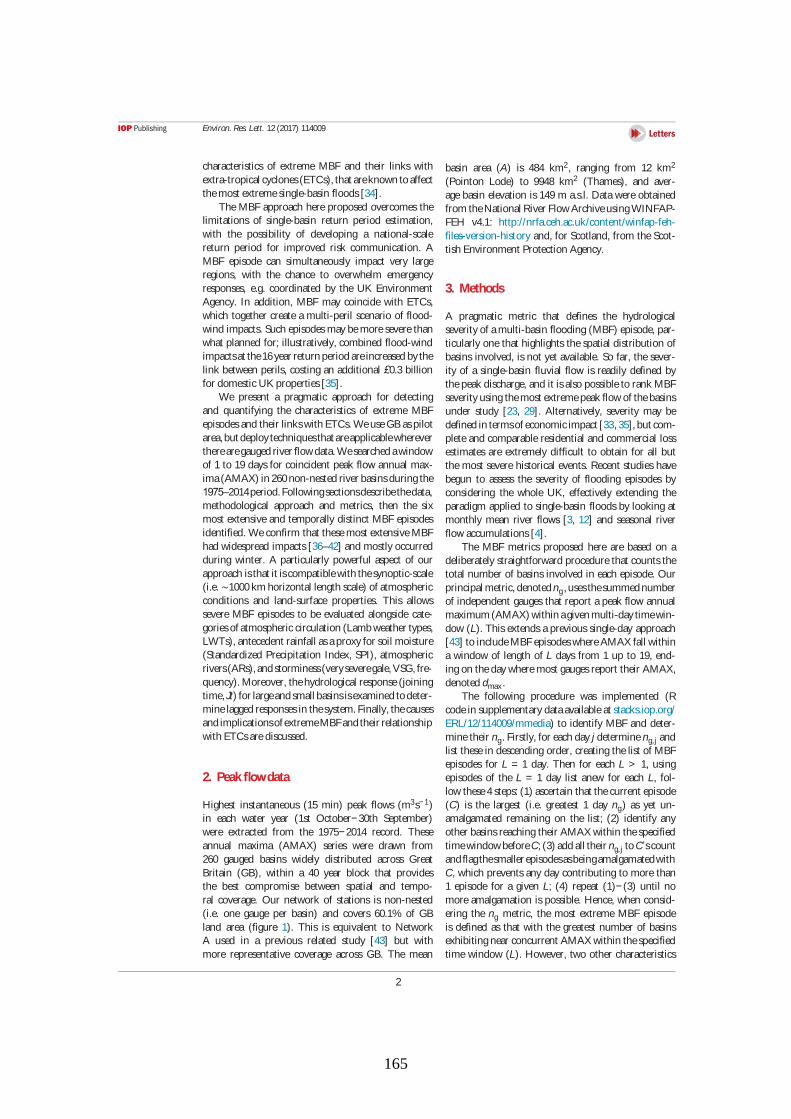
165

Environ. Res. Lett. 12(2017) 114009

characteristics of extreme MBF and their links with

extra-tropical cyclones(ETCs), that areknown toaffect

themost extremesingle-basin floods[34].

The MBF approach here proposed overcomes the

limitations of single-basin return period estimation,

with the possibility of developing a national-scale

return period for improved risk communication. A

MBF episode can simultaneously impact very large

regions, with the chance to overwhelm emergency

responses, e.g. coordinated by the UK Environment

Agency. In addition, MBF may coincide with ETCs,

which together create a multi-peril scenario of flood-

wind impacts. Such episodesmay bemoreseverethan

what planned for; illustratively, combined flood-wind

impactsat the16year return period areincreased bythe

link between perils, costing an additional £0.3 billion

for domestic UK properties[35].

We present a pragmatic approach for detecting

and quantifying the characteristics of extreme MBF

episodesand their linkswith ETCs. WeuseGBaspilot

area,but deploytechniquesthat areapplicablewherever

therearegauged river flowdata.Wesearchedawindow

of 1 to 19 days for coincident peak flow annual max-

ima(AMAX) in 260non-nested river basinsduringthe

1975–2014period.Followingsectionsdescribethedata,

methodological approach and metrics, then the six

most extensive and temporally distinct MBF episodes

identified. Weconfirm that thesemost extensiveMBF

had widespread impacts [36–42] and mostly occurred

during winter. A particularly powerful aspect of our

approach isthat it iscompatiblewith thesynoptic-scale

(i.e. ∼1000km horizontal length scale) of atmospheric

conditions and land-surface properties. This allows

severe MBF episodes to be evaluated alongside cate-

goriesof atmospheric circulation (Lambweather types,

LWTs), antecedent rainfall asaproxy for soil moisture

(Standardized Precipitation Index, SPI), atmospheric

rivers(ARs),andstorminess(veryseveregale,VSG, fre-

quency). Moreover, thehydrological response(joining

time,Jt) for largeandsmall basinsisexamined todeter-

minelagged responsesin thesystem. Finally, thecauses

andimplicationsof extremeMBFandtheir relationship

with ETCsarediscussed.

2. Peakflowdata

Highest instantaneous (15 min) peak flows (m3s−1)

in each water year (1st October−30th September)

were extracted from the 1975−2014 record. These

annual maxima (AMAX) series were drawn from

260 gauged basins widely distributed across Great

Britain (GB), within a 40 year block that provides

the best compromise between spatial and tempo-

ral coverage. Our network of stations is non-nested

(i.e. one gauge per basin) and covers 60.1% of GB

land area (figure 1). This is equivalent to Network

A used in a previous related study [43] but with

more representative coverage across GB. The mean

basin area (A) is 484 km2, ranging from 12 km2

(Pointon Lode) to 9948 km2 (Thames), and aver-

age basin elevation is 149 m a.s.l. Data were obtained

from theNational River Flow ArchiveusingWINFAP-

FEH v4.1: http://nrfa.ceh.ac.uk/content/winfap-feh-

files-version-history and, for Scotland, from the Scot-

tish Environment Protection Agency.

3. Methods

A pragmatic metric that defines the hydrological

severity of amulti-basin flooding (MBF) episode, par-

ticularly one that highlights the spatial distribution of

basins involved, is not yet available. So far, the sever-

ity of a single-basin fluvial flow is readily defined by

thepeak discharge, and it isalso possibleto rank MBF

severity using themost extremepeak flow of thebasins

under study [23, 29]. Alternatively, severity may be

defined in termsof economicimpact [33,35],but com-

plete and comparable residential and commercial loss

estimates are extremely difficult to obtain for all but

the most severe historical events. Recent studies have

begun to assess the severity of flooding episodes by

considering the whole UK, effectively extending the

paradigm applied to single-basin floods by looking at

monthly mean river flows [3, 12] and seasonal river

flow accumulations[4].

The MBF metrics proposed here are based on a

deliberately straightforward procedure that countsthe

total number of basins involved in each episode. Our

principal metric, denotedng,usesthesummednumber

of independent gauges that report a peak flow annual

maximum (AMAX) within agivenmulti-daytimewin-

dow (L). Thisextends aprevious single-day approach

[43] to includeMBFepisodeswhereAMAX fall within

a window of length of L days from 1 up to 19, end-

ing on theday wheremost gaugesreport their AMAX,

denoted dmax.

The following procedure was implemented (R

codein supplementary dataavailableat stacks.iop.org/

ERL/12/114009/mmedia) to identify MBF and deter-

minetheir ng. Firstly, for each day j determineng,j and

list these in descending order, creating the list of MBF

episodes for L = 1 day. Then for each L > 1, using

episodes of the L = 1 day list anew for each L, fol-

low these4steps: (1) ascertain that thecurrent episode

(C) is the largest (i.e. greatest 1 day ng) as yet un-

amalgamated remaining on the list; (2) identify any

other basinsreaching their AMAX within thespecified

timewindowbeforeC; (3) add all their ng,j toC’scount

andflagthesmaller episodesasbeingamalgamatedwith

C, which prevents any day contributing to more than

1 episode for a given L; (4) repeat (1)− (3) until no

more amalgamation is possible. Hence, when consid-

ering the ng metric, the most extreme MBF episode

is defined as that with the greatest number of basins

exhibitingnear concurrent AMAX within thespecified

time window (L). However, two other characteristics

2

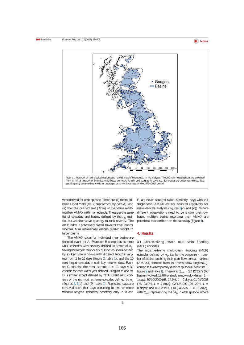
166


Figure1. Network of hydrological stationsand related areasof basinsused in theanalyses. The260 non-nested gaugeswereselectedfrom an initial network of 648 (figureS1) based on record length, and geographic coverage. Someareasareunder-represented (e.g.east England) because they areeither ungauged or do not havedatafor the1975−2014 period.

werederived for each episode. Theseare: (i) themulti-

basin Flood Yield (mFY, supplementary data A); and

(ii) the total drained area (TDA) of the basins reach-

ing their AMAX within an episode. Theseusethesame

list of episodes, and basins, defined by the ng met-

ric, but an alternative quantity to rank severity. The

mFY index is potentially biased towards small basins,

whereas TDA intrinsically assigns greater weight to

larger basins.

The AMAX dates for individual river basins are

denoted event set A. Event set B comprises extreme

MBF episodes with severity defined in terms of ng,

taking the largest temporally distinct episodesdefined

by six key time windows with different lengths, vary-

ing from 1 to 16 days (figure 2, table 1), and the 10

next largest episodes in each key time window. Event

set C contains the most extreme L = 13 days MBF

episodefor each water year defined usingmFY, and set

D is similar except defined by TDA. Event set E con-

sists of the six most extreme episodes defined by ng

(figures 2, 3(a) and (b), table 1). Replicated days are

removed such that days occurring in two or more

window lengths’ episodes, necessary only in B and

E, are never counted twice. Similarly, days with > 1

single-basin AMAX are not counted repeatedly for

national-scale analyses (figures 3(c) and (d)). Where

different observations need to be shown basin-by-

basin, multiple basins recording their AMAX are

permitted to contributeon thesameday (figure4).

4. Results

4.1. Characterizing severe multi-basin flooding

(MBF) episodes

The most extreme multi-basin flooding (MBF)

episodes defined by ng, i.e. by the concurrent num-

ber of basins reaching their peak flow annual maxima

(AMAX), obtained from 19 timewindow lengths (L),

comprisefivetemporally distinct episodes(event set E,

figure2and table1). Theseare: dmax = 27/12/1979(66

basinsinvolved,18.6%of studyarea,windowlengthL=

1day); 30/10/2000(68, 14.1%, L = 2days); 01/01/2003

(75, 24.9%, L = 4 days); 02/12/1992 (96, 22%, L =

8 days); and 01/02/1995 (108, 46.5%, L = 16 days),

with dmax representing theday, in each episode, where

3

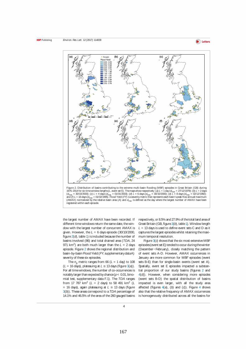
167


(a) (b) (c)

(d) (e) (f)

Figure 2. Distribution of basins contributing to the extreme multi-basin flooding (MBF) episodes in Great Britain (GB) during1975–2014 for six timewindow lengths(L, event set E). Themapsshowrespectively: (a) L = 1day (dmax = 27/12/1979); (b) L = 2days(dmax = 30/10/2000); (c) L = 4 days (dmax = 01/01/2003); (d) L = 6 days (dmax = 30/10/2000); (e) L = 8 days(dmax = 02/12/1992);and (f) L = 16days(dmax = 01/02/1995). Flood Yield (FY) isaseverity metric that representseach basin’speak flowannual maximum(AMAX) normalized by the relative basin area (A) and dmax is defined as the day where the largest number of AMAX have beenregistered within each episode.

the largest number of AMAX have been recorded. If

different timewindowsreturn thesamedate, thewin-

dow with the largest number of concurrent AMAX is

given. However, the L = 6 days episode (30/10/2000,

figure2(d), table1) is included becausethenumber of

basins involved (86) and total drained area (TDA, 24

971 km2) are both much larger than the L = 2 days

episode. Figure 2 shows the regional distribution and

basin-by-basin FloodYield (FY,supplementarydataA)

severity of thesesix episodes.

The ng metric ranges from 66 (L = 1 day) to 108

(L = 16 days), plateauing at L ≅ 13 days (figure 3(a)).

For all timewindows, thenumber of co-occurrences is

notably larger than expectedbychance(p< 0.01, bino-

mial test, supplementary data F.1). The TDA ranges

from 17 787 km2 (L = 2 days) to 58 491 km2 (L

= 16 days), again plateauing at L ≅ 13 days (figure

3(b)). Theseareascorrespond to aTDA percentageof

14.1% and 46.5% of thearea of the260 gauged basins

respectively, or 8.5%and 27.9%of thetotal land areaof

Great Britain (GB, figure3(b), table1).Window length

L = 13 days is used to define event sets C and D as it

capturesthelargest episodeswhilst retaining themaxi-

mum temporal resolution.

Figure3(c) showsthat thesix most extensiveMBF

episodes(event set E) tended tooccur duringthewinter

(December−February), closely matching the pattern

of event sets A-D. However, AMAX occurrences in

January are more common for MBF episodes (event

sets B-E) than for single-basin events (event set A).

Spatially, event set E episodes impacted a substan-

tial proportion of our study basins (figures 2 and

4(d)). However, when considering more episodes

(event sets B-D) the spatial distribution of basins

impacted is even larger, with all the study area

affected (figures 4(a), (b) and (c)). Figure 4 shows

also that therelative frequency of AMAX occurrences

is homogenously distributed across all the basins for

4

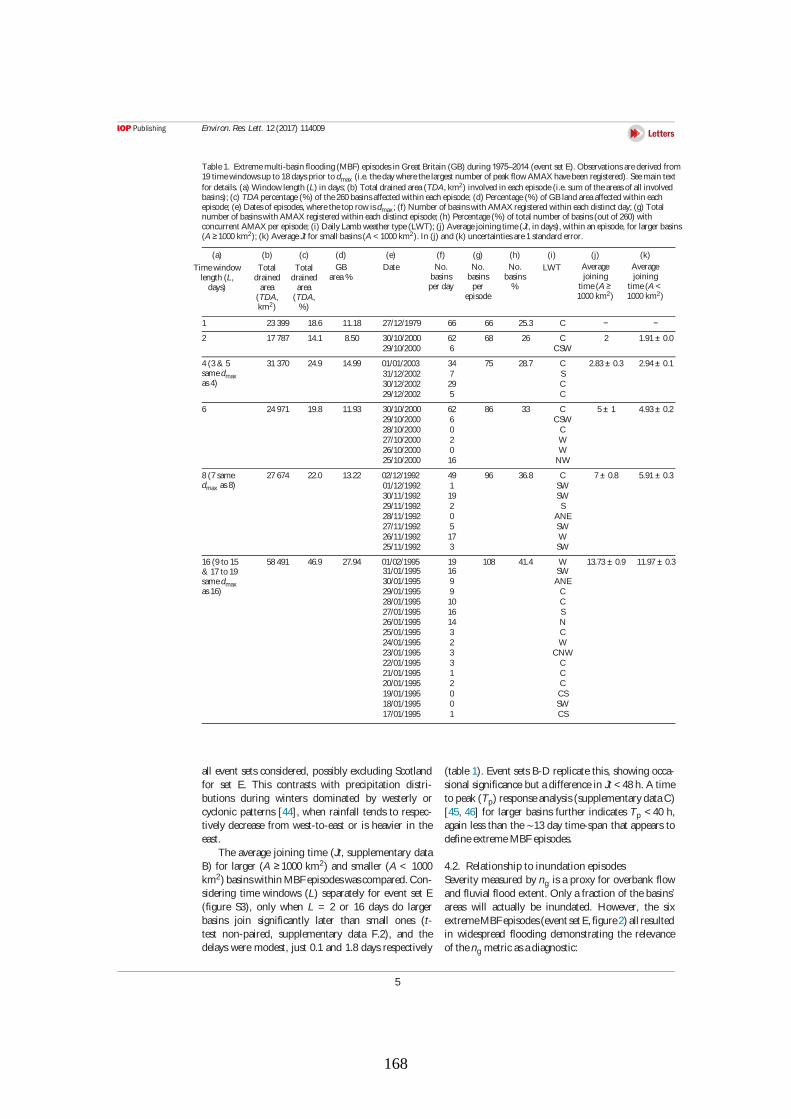
168


Table1. Extrememulti-basin flooding(MBF) episodesin Great Britain (GB) during1975–2014 (event set E). Observationsarederived from19 timewindowsup to 18daysprior to dmax (i.e. theday wherethelargest number of peak flow AMAX havebeen registered). Seemain text

for details. (a) Window length (L) in days; (b) Total drained area(TDA, km2) involved in each episode(i.e. sum of theareasof all involvedbasins); (c) TDA percentage(%) of the260 basinsaffected within each episode; (d) Percentage(%) of GBland areaaffected within eachepisode; (e) Datesof episodes, wherethetop row isdmax; (f) Number of basinswith AMAX registered within each distinct day; (g) Totalnumber of basinswith AMAX registered within each distinct episode; (h) Percentage(%) of total number of basins(out of 260) withconcurrent AMAX per episode; (i) Daily Lamb weather type(LWT); (j) Averagejoiningtime(Jt, in days), within an episode, for larger basins(A ≥1000 km2); (k) AverageJt for small basins(A < 1000 km2). In (j) and (k) uncertaintiesare1 standard error.

(a) (b) (c) (d) (e) (f) (g) (h) (i) (j) (k)

Timewindowlength (L,

days)

Totaldrained

area(TDA,km2)

Totaldrained

area(TDA,

%)

GBarea%

Date No.basinsper day

No.basins

perepisode

No.basins

%

LWT Averagejoining

time(A ≥1000 km2)

Averagejoining

time(A <1000 km2)

1 23 399 18.6 11.18 27/12/1979 66 66 25.3 C − −

2 17 787 14.1 8.50 30/10/2000 62 68 26 C 2 1.91± 0.0

29/10/2000 6 CSW

4(3& 5samedmax

as4)

31 370 24.9 14.99 01/01/2003 34 75 28.7 C 2.83± 0.3 2.94± 0.1

31/12/2002 7 S30/12/2002 29 C

29/12/2002 5 C

6 24 971 19.8 11.93 30/10/2000 62 86 33 C 5± 1 4.93± 0.2

29/10/2000 6 CSW

28/10/2000 0 C

27/10/2000 2 W26/10/2000 0 W

25/10/2000 16 NW

8(7samedmax as8)

27 674 22.0 13.22 02/12/1992 49 96 36.8 C 7± 0.8 5.91± 0.3

01/12/1992 1 SW30/11/1992 19 SW

29/11/1992 2 S

28/11/1992 0 ANE

27/11/1992 5 SW

26/11/1992 17 W25/11/1992 3 SW

16 (9 to 15& 17 to 19samedmax

as16)

58 491 46.9 27.94 01/02/1995 19 108 41.4 W 13.73 ± 0.9 11.97 ± 0.331/01/1995 16 SW

30/01/1995 9 ANE

29/01/1995 9 C

28/01/1995 10 C

27/01/1995 16 S26/01/1995 14 N

25/01/1995 3 C

24/01/1995 2 W

23/01/1995 3 CNW

22/01/1995 3 C21/01/1995 1 C

20/01/1995 2 C

19/01/1995 0 CS18/01/1995 0 SW

17/01/1995 1 CS

all event sets considered, possibly excluding Scotland

for set E. This contrasts with precipitation distri-

butions during winters dominated by westerly or

cyclonic patterns [44], when rainfall tends to respec-

tively decrease from west-to-east or is heavier in the

east.

The average joining time (Jt, supplementary data

B) for larger (A ≥1000 km2) and smaller (A < 1000

km2) basinswithin MBFepisodeswascompared. Con-

sidering time windows (L) separately for event set E

(figure S3), only when L = 2 or 16 days do larger

basins join significantly later than small ones (t-

test non-paired, supplementary data F.2), and the

delays were modest, just 0.1 and 1.8 days respectively

(table 1). Event sets B-D replicate this, showing occa-

sional significancebut adifference in Jt < 48 h. A time

to peak (Tp) responseanalysis(supplementary dataC)

[45, 46] for larger basins further indicates Tp < 40 h,

again less than the ∼13 day time-span that appears to

defineextremeMBF episodes.

4.2. Relationship to inundation episodes

Severity measured by ng is a proxy for overbank flow

and fluvial flood extent. Only a fraction of thebasins’

areas will actually be inundated. However, the six

extremeMBFepisodes(event set E,figure2) all resulted

in widespread flooding demonstrating the relevance

of theng metric asadiagnostic:

5

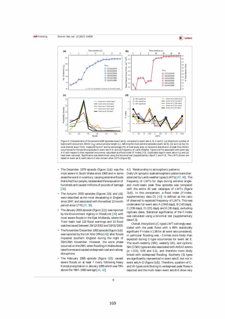
169


1 4 7 10 13 16 19

60

70

80

90

100

110

No.

of B

asin

s (n

g)

Time window (L)

p < 0.01 of 1 top episode in 40 years, for all window lengths

(a)

dmax

27/12/1979

30/10/2000

01/01/2003

30/10/2000

02/12/1992

01/02/1995

1 4 7 10 13 16 19

2.0

2.5

3.0

3.5

4.0

4.5

5.0

5.5

6.0

To

tal D

rain

ed

Are

a (TDA

, km

2 *

10

4)

Time window (L)(b)

dmax

27/12/1979

30/10/2000

01/01/2003

30/10/2000

02/12/1992

01/02/1995

1 4 7 10 13 16 19

14

17

20

23

26

29

32

35

38

41

44

47

% T

ota

l B

asin

s A

rea

0.0

0.1

0.2

0.3

0.4

0.5

Pro

ba

bili

ty D

en

sity

Month

Oct Dec Feb Apr Jun Aug

(c)

Event set A (2443 days)

Event set B (143 days)

Event set C (239 days)

Event set D (221 days)

Event set E (30 days)

01

23

4

LWTs

FIn

dex

C SW W CSW S NW CS A N CNW

(d)

Event set A (2443 days)

Event set B (143 days)

Event set C (239 days)

Event set D (221 days)

Event set E (30 days)

99% significant

95% significant

90% significant

Figure3. Characteristicsof theextremeMBFepisodes(event set E), compared to event setsA, B, C and D. (a) Maximum number ofbasinswith concurrent AMAX (ng) versuswindow length (L), defining themost extremeepisodes(event set E); (b) asin (a) but for

total drained area(TDA), measured by km2 and by percentage(%) of total study area; (c) temporal distribution of peak flow AMAXoccurrences for theextremeepisodesin event setsA-E; and (d) frequency of Lamb Weather Types(LWTs) associated with event setsA-Ewith respect to their expected occurrence, calculated asaflood index (F-Index) [43]. Duplicated daysin event setsin (c) and (d)have been removed. Significance was determined using the binomial test (supplementary data F.1 and F.3). The LWTsshown arebased on event set E; event setsA-D also contain other LWTs(figureS2).

• The December 1979 episode (figure 2(a)) was the

most severe in South Walessince1960 and in some

areastheworst in acentury, causingextensivefloods

that killedfour people,necessitatedtheevacuationof

hundredsand caused millionsof poundsof damage

[36].

• The Autumn 2000 episodes (figures 2(b) and (d))

were described as the most devastating in England

since1947, and associated with thewettest 12month

period since1776 [37, 38].

• TheJanuary 2003episode(figure2(c)) wasreported

by theEnvironment Agency in FloodLink [39] with

most severe floods in the East Midlands, where the

Trent basin had 118 flood warnings and 14 flood

watchesissued between 29/12/2002and 03/01/2003.

• TheNovember/December 1992episode(figure2(e))

wasreported by theUK Met Office[40] after floods

impacted southern England during the night of

25th/26th November. However, the worst phase

occurred on the29th,when flooding in Walesdevas-

tatedhomesandcausedwidespreadroadandrailway

disruptions.

• The February 1995 episode (figure 2(f)) caused

severe floods on at least 7 rivers, following heavy

frontal precipitation in January1995which was79%

abovethe1961–1990average[41, 42].

4.3. Relationship to atmospheric patterns

DailyUK synoptic-scaleatmosphericpatternsarechar-

acterized by Lamb weather types(LWTs) [47, 48]. The

frequency of LWTs for days during extreme single-

and multi-basin peak flow episodes was compared

with the entire 40 year catalogue of LWTs (figure

3(d)). In this comparison, a flood index (F-Index,

supplementary data D) [43] is defined as the ratio

of observed to expected frequency of LWTs. Thiswas

undertaken for event sets: A (2443days), B (143days),

C (239 days), D (221 days) and E(30 days), excluding

replicate dates. Statistical significance of the F-Index

was calculated using a binomial test (supplementary

dataF.3).

Overall, thecyclonic(C-type) LWT isstronglyasso-

ciated with the peak flows with a 99% statistically

significant F-Index ≥1.98 for all event setsconsidered,

in particular flooding was ∼3 times more likely than

expected during C-type occurrences for event set E.

The south-westerly (SW), westerly (W), and cyclonic

SW (CSW) typesarealsoassociatedwithAMAX events

(p < 0.01, 0.05 and 0.1), and therefore more likely

linked with widespread flooding. Southerly (S) types

aresignificantly represented in event setsE, but not in

event setsA-D (figure3(d)). Therefore, apattern of C-

and W-typescontributing to widespread peak flows is

depicted and themulti-basin event setsB-E show very

6

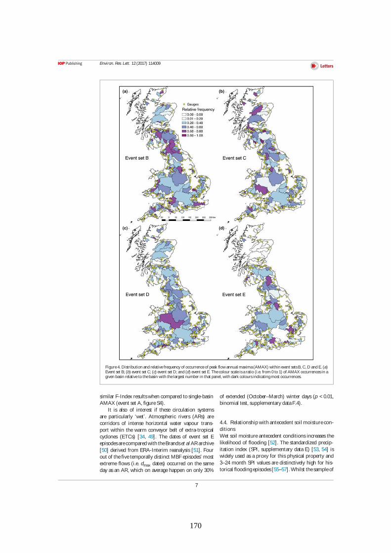
170


(a) (b)

(c) (d)

Figure4. Distribution and relativefrequency of occurrenceof peak flowannual maxima(AMAX) within event setsB, C, D and E. (a)Event set B; (b) event set C; (c) event set D; and (d) event set E. Thecolour scaleisaratio (i.e. from 0 to 1) of AMAX occurrencesin agiven basin relativeto thebasin with thelargest number in that panel, with dark coloursindicatingmost occurrences.

similar F-Index resultswhen compared to single-basin

AMAX (event set A, figureS4).

It is also of interest if these circulation systems

are particularly ‘wet’. Atmospheric rivers (ARs) are

corridors of intense horizontal water vapour trans-

port within the warm conveyor belt of extra-tropical

cyclones (ETCs) [34, 49]. The dates of event set E

episodesarecompared with theBrandset al ARarchive

[50] derived from ERA-Interim reanalysis [51]. Four

out of thefivetemporally distinct MBF episodes’ most

extreme flows (i.e. dmax dates) occurred on the same

day asan AR, which on average happen on only 30%

of extended (October–March) winter days (p < 0.01,

binomial test, supplementary dataF.4).

4.4. Relationship with antecedent soil moisturecon-

ditions

Wet soil moistureantecedent conditions increases the

likelihood of flooding [52]. The standardized precip-

itation index (SPI, supplementary data E) [53, 54] is

widely used as a proxy for this physical property and

3–24 month SPI values are distinctively high for his-

torical floodingepisodes[55–57]. Whilst thesampleof

7

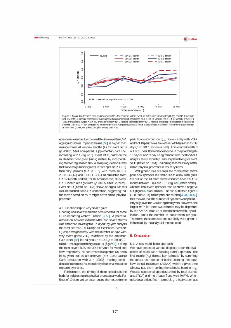
171


Time Windows (L)

SP

I m

ea

n

0.3

0.0

0.3

0.6

0.9

1.2

1.5

1 day 2 day 4 day 6 day 8 day 16 day

Overall SPI 24 Month

SPI 18 Month

SPI 12 Month

SPI 6 Month

SPI 3 Month

SPI 1 Month

All SPI observations significant with p << 0.01

Figure5. Mean standardized precipitation index (SPI) for episodeswithin event set B for each window length (L) and SPI timescale(24-1Month). Linesareepisodes’ SPI averageswith coloursindicating: dashed blue= SPI 24 Month; red = SPI 18Month; grey = SPI12Month;dashed purple= SPI 6Month;dark blue= SPI 3Month;dashed brown = SPI 1Month.Theblack linerepresentstheoverall(40 year ,1975–2014) SPI averagei.e. zero bydefinition. All episodeshaveSPI that aresignificantlydifferent from thelong-term meanat 99% level (t-test, not paired, supplementary dataF.5).

episodesinevent set Eistoosmall toshowapattern,SPI

aggregated across impacted basins [58] ishigher than

average across all window lengths (L) for event set B

(p ≪ 0.01, t-test non-paired, supplementary dataF.5),

increasing with L (figure5). Event set C, based on the

multi-basin flood yield (mFY) metric, by incorporat-

ingaforcedregularized annual sampling,demonstrates

that floodmagnitudeisgreater in ‘wet’ spells(SPI > 0.5)

than ‘dry’ periods (SPI < −0.5) with mean mFY =

26.9±3.4 (1 ) and 17.1±1.3 (1 ) as calculated from

SPI 12 Month. Indeed, for thiscomparison, all except

SPI 1 Month aresignificant (p < 0.05, t-test, 2-tailed).

Event set D (based on TDA) shows no signal for this

well-established flood-SPI connection, suggesting that

themetric based on mFY might better reflect physical

processes.

4.5. Relationship to very severegales

Flooding and severewind havebeen reported for some

ETCs impacting western Europe [3, 59]. A potential

association between extreme MBF and severe storms

was, therefore, investigated. In a year-by-year analysis

themost extremeL = 13 daysmFY episodes(event set

C) correlates positively with the number of days with

very severe gales (VSG) as defined by the Jenkinson

Gale Index [48] in that year (r = 0.41, p = 0.0088, 2-

tailed t-test, supplementarydataF.6) (figure6). Taking

the most severe 50% and 30% of years for wind and

flow respectively, co-occurrence is expected 6.0 times

in 40 years, but 10 are observed (p = 0.021; Monte

Carlo simulation with n = 10000), making coinci-

denceof extremes67% morelikely than what would be

expected by chance.

Furthermore, the timing of these episodes is the

basisfor insightsintothephysical processesat work.For

5out of 10observed co-occurrences, themost extreme

peak flows recorded on dmax are on a day with VSG,

and 9of 10peak flowsarewithin 0–13daysafter aVSG

day (p ≪ 0.001, binomial test). This contrasts with 0

out of 10peak flow episodesfound in thepreceding 0–

13daysof aVSG day. In agreement with theflood-SPI

analysis, therelationship isnotably lessstrongfor event

set D (based on TDA), indicating that mFYmay better

reflect physical processes in storm systems.

Wet ground is a pre-requisite to the most severe

peak flow episodes, but there is also a link with gales.

Six out of the 10 most severe episodes have a SPI 12

month between +0.4and +1.1(figure6, whitecircles),

whereas less severe episodes tend to show a negative

SPI (figure6, black circles). Thetwo outliersin figure6

(1983 and 2014) reflect previousstudies[4, 44, 60–63]

that showed that thenumber of cycloneswereparticu-

larly high over theGBduring theseyears. However, the

largest mFY for these two episodes may be depressed

by theAMAX measure of extremeness which, by def-

inition, limits the number of occurrences per year.

Therefore, these observations are likely valid given, if

influenced by theanalytical method used.

5. Discussion

5.1. A new multi-basin approach

We have presented various diagnostics for the eval-

uation of multi-basin flooding (MBF) episodes. The

first metric (ng) detects key ‘episodes’ by summing

the concurrent number of basins attaining their peak

flow annual maximum (AMAX) within a given time

window (L), then ranking the episodes based on ng.

We also considered episodes ranked by total drained

area (TDA) and multi-basin flood yield (mFY). When

episodesareidentified in termsof ng, thisgivesperhaps

8

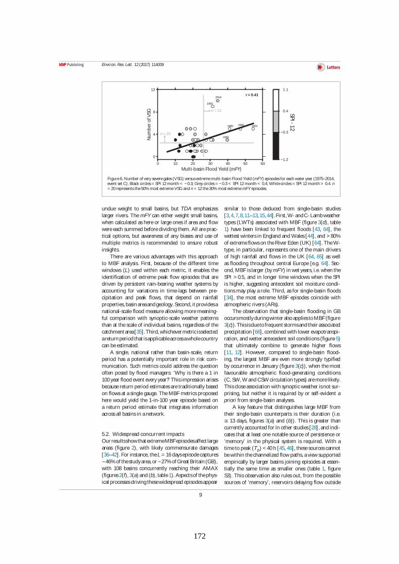
172


0

4

8

12

6050403020100−1.2

−0.3

0.4

1.1

SPI - 1

2

Nu

mb

er o

f VSG

Multi-basin Flood Yield (mFY)

n = 20

n = 12

2001

1993

1980 1999

1983

2014r = 0.41

Figure6. Number of very severegales(VSG) versusextrememulti-basin Flood Yield (mFY) episodesfor each water year (1975–2014,event set C). Black circles= SPI 12month < −0.3; Grey circles= −0.3 < SPI 12 month < 0.4; Whitecircles= SPI 12 month > 0.4. n= 20 representsthe50% most extremeVSG and n = 12 the30% most extrememFYepisodes.

undue weight to small basins, but TDA emphasizes

larger rivers. The mFY can either weight small basins,

when calculated as here or large ones if area and flow

wereeach summed beforedividing them. All areprac-

tical options, but awareness of any biases and use of

multiple metrics is recommended to ensure robust

insights.

There are various advantages with this approach

to MBF analysis. First, because of the different time

windows (L) used within each metric, it enables the

identification of extreme peak flow episodes that are

driven by persistent rain-bearing weather systems by

accounting for variations in time-lags between pre-

cipitation and peak flows, that depend on rainfall

properties,basinareaandgeology.Second, it providesa

national-scale flood measureallowing moremeaning-

ful comparison with synoptic-scale weather patterns

than at thescaleof individual basins, regardless of the

catchment area[35].Third,whichevermetricisselected

areturnperiod that isapplicableacrossawholecountry

can beestimated.

A single, national rather than basin-scale, return

period has a potentially important role in risk com-

munication. Such metrics could address the question

often posed by flood managers: ‘Why is there a 1 in

100year flood event everyyear?’ Thisimpression arises

becausereturn period estimatesaretraditionally based

on flowsat asingle gauge. TheMBF metricsproposed

here would yield the 1-in-100 year episode based on

a return period estimate that integrates information

acrossall basins in anetwork.

5.2. Widespread concurrent impacts

Our resultsshowthat extremeMBFepisodesaffect large

areas (figure 2), with likely commensurate damages

[36–42]. For instance, theL = 16daysepisodecaptures

∼46%of thestudyarea,or ∼27%of Great Britain (GB),

with 108 basins concurrently reaching their AMAX

(figures2(f), 3(a) and (b), table1). Aspectsof thephys-

ical processesdrivingthesewidespread episodesappear

similar to those deduced from single-basin studies

[3,4,7,8,11–13,15,44].First,W- andC- Lambweather

types (LWTs) associated with MBF (figure 3(d), table

1) have been linked to frequent floods [43, 64], the

wettest wintersin England and Wales[44], and > 80%

of extremeflowson theRiver Eden (UK) [64]. TheW-

type, in particular, represents one of themain drivers

of high rainfall and flows in the UK [64, 65] as well

as flooding throughout central Europe [e.g. 64]. Sec-

ond, MBFislarger (bymFY) in wet years, i.e. when the

SPI > 0.5, and in longer time windows when the SPI

is higher, suggesting antecedent soil moisture condi-

tionsmay play arole. Third, asfor single-basin floods

[34], the most extreme MBF episodes coincide with

atmospheric rivers(ARs).

The observation that single-basin flooding in GB

occursmostlyduringwinter alsoappliestoMBF(figure

3(c)).Thisisduetofrequent stormsandtheir associated

precipitation [66], combined with lower evapotranspi-

ration, and wetter antecedent soil conditions(figure5)

that ultimately combine to generate higher flows

[11, 12]. However, compared to single-basin flood-

ing, the largest MBF are even more strongly typified

by occurrence in January (figure3(c)), when themost

favourable atmospheric flood-generating conditions

(C, SW, W and CSW circulation types) aremorelikely.

Thiscloseassociation with synopticweather isnot sur-

prising, but neither it is required by or self-evident a

priori from single-basin analyses.

A key feature that distinguishes large MBF from

their single-basin counterparts is their duration (i.e.

≅ 13 days, figures 3(a) and (b)). This is greater than

currently accounted for in other studies[28], and indi-

cates that at least one notable source of persistence or

‘memory’ in the physical system is required. With a

timeto peak (Tp) < 40h [45, 46], thesesourcescannot

bewithin thechannelized flow paths, aview supported

empirically by larger basins joining episodes at essen-

tially the same time as smaller ones (table 1, figure

S3). Thisobservation also rulesout, from thepossible

sources of ‘memory’, reservoirs delaying flow outside

9

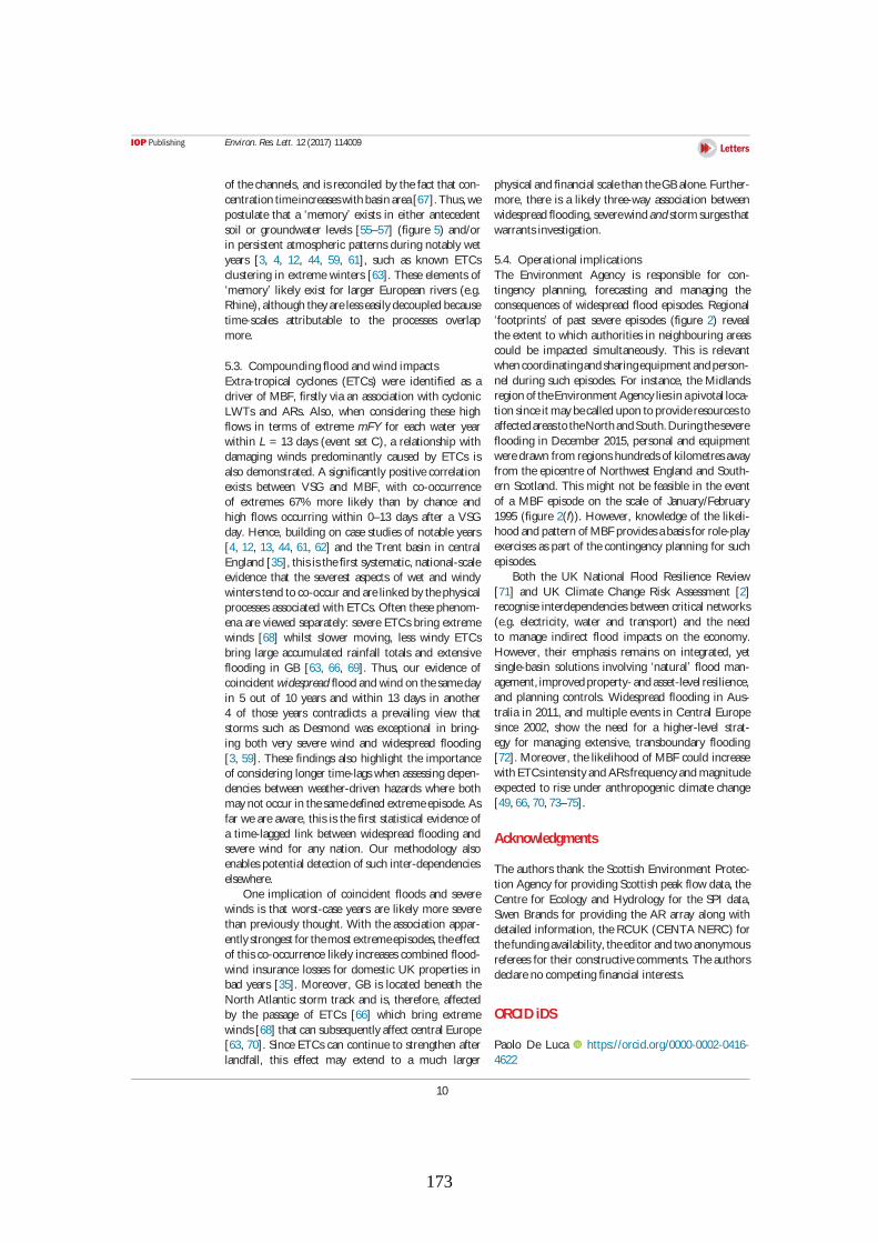
173


of thechannels, and isreconciled by thefact that con-

centration timeincreaseswithbasin area[67].Thus,we

postulate that a ‘memory’ exists in either antecedent

soil or groundwater levels [55–57] (figure 5) and/or

in persistent atmospheric patterns during notably wet

years [3, 4, 12, 44, 59, 61], such as known ETCs

clustering in extreme winters [63]. These elements of

‘memory’ likely exist for larger European rivers (e.g.

Rhine), although theyarelesseasilydecoupled because

time-scales attributable to the processes overlap

more.

5.3. Compoundingflood and wind impacts

Extra-tropical cyclones (ETCs) were identified as a

driver of MBF, firstly via an association with cyclonic

LWTs and ARs. Also, when considering these high

flows in terms of extreme mFY for each water year

within L = 13 days (event set C), a relationship with

damaging winds predominantly caused by ETCs is

also demonstrated. A significantly positivecorrelation

exists between VSG and MBF, with co-occurrence

of extremes 67% more likely than by chance and

high flows occurring within 0–13 days after a VSG

day. Hence, building on case studies of notable years

[4, 12, 13, 44, 61, 62] and the Trent basin in central

England [35], thisisthefirst systematic, national-scale

evidence that the severest aspects of wet and windy

winterstend to co-occur and arelinked by thephysical

processes associated with ETCs. Often thesephenom-

ena are viewed separately: severe ETCs bring extreme

winds [68] whilst slower moving, less windy ETCs

bring large accumulated rainfall totals and extensive

flooding in GB [63, 66, 69]. Thus, our evidence of

coincident widespread flood and wind on thesameday

in 5 out of 10 years and within 13 days in another

4 of those years contradicts a prevailing view that

storms such as Desmond was exceptional in bring-

ing both very severe wind and widespread flooding

[3, 59]. These findings also highlight the importance

of considering longer time-lagswhen assessing depen-

dencies between weather-driven hazards where both

maynot occur in thesamedefined extremeepisode. As

far weare aware, this is thefirst statistical evidence of

a time-lagged link between widespread flooding and

severe wind for any nation. Our methodology also

enablespotential detection of such inter-dependencies

elsewhere.

One implication of coincident floods and severe

winds is that worst-case years are likely more severe

than previously thought. With the association appar-

entlystrongest for themost extremeepisodes, theeffect

of thisco-occurrence likely increasescombined flood-

wind insurance losses for domestic UK properties in

bad years [35]. Moreover, GB is located beneath the

North Atlantic storm track and is, therefore, affected

by the passage of ETCs [66] which bring extreme

winds[68] that can subsequently affect central Europe

[63, 70]. Since ETCs can continue to strengthen after

landfall, this effect may extend to a much larger

physical and financial scalethan theGBalone. Further-

more, there is a likely three-way association between

widespread flooding,severewind andstorm surgesthat

warrantsinvestigation.

5.4. Operational implications

The Environment Agency is responsible for con-

tingency planning, forecasting and managing the

consequences of widespread flood episodes. Regional

‘footprints’ of past severe episodes (figure 2) reveal

the extent to which authorities in neighbouring areas

could be impacted simultaneously. This is relevant

whencoordinatingandsharingequipment andperson-

nel during such episodes. For instance, the Midlands

region of theEnvironment Agencyliesin apivotal loca-

tion sinceit maybecalled upon to provideresourcesto

affectedareastotheNorthandSouth.Duringthesevere

flooding in December 2015, personal and equipment

weredrawn from regionshundredsof kilometresaway

from the epicentre of Northwest England and South-

ern Scotland. This might not be feasible in the event

of a MBF episode on the scale of January/February

1995 (figure 2(f)). However, knowledge of the likeli-

hood and pattern of MBFprovidesabasisfor role-play

exercises as part of thecontingency planning for such

episodes.

Both the UK National Flood Resilience Review

[71] and UK Climate Change Risk Assessment [2]

recognise interdependencies between critical networks

(e.g. electricity, water and transport) and the need

to manage indirect flood impacts on the economy.

However, their emphasis remains on integrated, yet

single-basin solutions involving ‘natural’ flood man-

agement, improvedproperty- andasset-level resilience,

and planning controls. Widespread flooding in Aus-

tralia in 2011, and multiple events in Central Europe

since 2002, show the need for a higher-level strat-

egy for managing extensive, transboundary flooding

[72]. Moreover, the likelihood of MBF could increase

with ETCsintensityand ARsfrequencyand magnitude

expected to rise under anthropogenic climate change

[49, 66, 70, 73–75].

Acknowledgments

The authors thank the Scottish Environment Protec-

tion Agency for providing Scottish peak flow data, the

Centre for Ecology and Hydrology for the SPI data,

Swen Brands for providing the AR array along with

detailed information, theRCUK (CENTA NERC) for

thefundingavailability, theeditor and twoanonymous

referees for their constructivecomments. Theauthors

declareno competingfinancial interests.

ORCIDiDS

Paolo De Luca https://orcid.org/0000-0002-0416-

4622

10

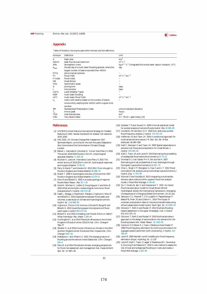
174


Appendix

Tableof Notation Acronymsused within thetext and full definition.

Acronym Definition Unit

A basin area km2

AMAX peak flow annual maximum m3 s−1

ARs atmospheric rivers kgm−1 s−1 (integrated horizontal water vapour transport, IVT)

d thelast day of amulti-basin floodingepisode, wherethe

largest number of basinsrecorded their AMAX

day

ETCs extra-tropical cyclones −

FY Flood Yield m3 s−1 km−2

F-Index Flood Index −

GB Great Britain −HAs hydrometricareas −

Jt joiningtime days

L timewindow days

LWTs Lamb Weather Types −

MBF multi-basin flooding −mFY multi-basin Flood Yield m3 s−1 km−2

n metricwith severity based on thenumber of basins

concurrently reaching their AMAX within agiven time

window

−

SPI Standardized Precipitation Index unitsof standard deviation

T timeto peak hoursTDA total drained area km2

VSG Very SevereGales G > 50 (G = galeindex) [48]

References

[1] UNISDR(United NationsInternational Strategy for Disaster

Reduction) 2015 Sendai framework for disaster risk reduction

2015–2030

[2] ASC 2016 UK ClimateChangeRisk Assessment 2017

SynthesisReport: prioritiesfor thenext fiveyearsAdaptation

Sub-Committeeof theCommitteeon ClimateChange,

London

[3] Barker L, Hannaford J, Muchan K, Turner Sand Parry S 2016

Thewinter 2015/2016 floodsin theUK: ahydrological

appraisal Weather 71324–33

[4] Muchan K, LewisM, Hannaford Jand Parry S 2015 The

winter stormsof 2013/2014 in theUK: hydrological responses

and impactsWeather 7055–61

[5] Parry S, Marsh T and Kendon M 2013 2012: From drought to

floodsin England and WalesWeather 68268–74

[6] Marsh T 2008 A hydrological overview of thesummer 2007

floodsin England and WalesWeather 63274–9

[7] MerzRand Bloschl G 2003 A processtypologyof regional

floodsWater Resour. Res. 39 1–20

[8] Nied M, Schroter K, LudtkeS, DungNguyen V and Merz B

2016 What arethehydro-meteorological controlson flood

characteristics?J. Hydrol. 545310–26

[9] Gaaıl L, Szolgay J, HlavcovaK, ParajkaJ, ViglioneA, Merz R

and Bloschl G 2015 Dependencebetween flood peaksand

volumes: acasestudy on climateand hydrological controls

Hydrol. Sci. J. 60968–84

[10] ViglioneA, Chirico G B, KommaJ, WoodsR, BorgaM and

Bloschl G 2010Quantifyingspace-timedynamicsof flood

event typesJ. Hydrol 394 213–29

[11] Bloschl G et al 2015 Increasing river floods: fiction or reality?

Wiley Interdiscip. Rev. Water 2329–44

[12] Huntingford C et al 2014 Potential influenceson theUnited

Kingdom’sfloodsof winter 2013/14 Nat. Clim. Change4

769–77

[13] Schaller N et al 2016Human influenceon climatein the2014

southern England winter floodsand their impactsNat. Clim.

Change6627–34

[14] Mallakpour I and Villarini G 2015 Thechangingnatureof

floodingacrossthecentral United StatesNat. Clim. Change5

250–4

[15] Merz B et al 2014 Floodsand climate: emergingperspectives

for flood risk assessment and management Nat. HazardsEarth

Syst. Sci. 141921–42

[16] Kjeldsen T Rand JonesD A 2009 A formal statistical model

for pooled analysisof extremefloodsHydrol. Res. 40465–80

[17] Cunderlik JM and Burn D H 2003 Non-stationarypooled

flood frequency analysisJ. Hydrol. 276 210–23

[18] Heffernan JEand Tawn JA 2004 A conditional approach for

multivariateextremevaluesJ. R. Stat. Soc. Ser. B Stat.

Methodol. 66497–530

[19] Keef C, Svensson C and Tawn JA 2009 Spatial dependencein

extremeriver flowsand precipitation for Great Britain J.

Hydrol. 378240–52

[20] Keef C, Tawn JA and Lamb R 2013Estimatingtheprobability

of widespread flood eventsEnvironmetrics2413–21

[21] DeWaal D J, Van Gelder PH A JM and Nel A 2007

Estimatingjoint tail probabilitiesof river dischargesthrough

thelogisticcopulaEnvironmetrics18621–31

[22] Chen L, Singh V P, Shenglian G, Hao Z and Li T 2012 Flood

coincidencerisk analysisusingmultivariatecopulafunctionsJ.

Hydrol. Eng. 17742–55

[23] Wyncoll D and Gouldby B 2013 Integratingamultivariate

extremevaluemethod within asystem flood risk analysis

model J. Flood Risk Manage. 8145–60

[24] Qu Y, Dodov B, Jain V and Hautaniemi T 2010 An inland

flood lossestimation model for Great Britain British

Hydrological Society 3rd International Symposium, Managing

Consequencesof a ChangingGlobal Environment, 19–23 July

[25] Sampson C C, Fewtrell T J, O’Loughlin F, Pappenberger F,

BatesPB, Freer JEand ClokeH L 2014Theimpact of

uncertain precipitation dataon insurancelossestimatesusing

aflood catastrophemodel Hydrol. Earth Syst. Sci. 182305–24

[26] Ghizzoni T, Roth G and Rudari R 2012 Multisiteflooding

hazard assessment in theupper Mississippi river J. Hydrol.

412–413 101–13

[27] Ghizzoni T, Roth G and Rudari R 2010 Multivariateskew-t

approach to thedesign of accumulation risk scenariosfor the

floodinghazard Adv. Water Resour. 331243–55

[28] Cameron D S, Beven K J, Tawn J, BlazkovaSand Naden P

1999 Flood frequency estimation by continuoussimulation for

agauged upland catchment (with uncertainty) J. Hydrol. 219

169–87

[29] Lamb R 2006 Rainfall-runoff modellingfor flood frequency

estimation Encycl. Hydrolog. Sci. 11 125

[30] Lamb R, Keef C, Tawn J, Laeger S, Meadowcroft I, Surendran

S, DunningPand BastoneC 2010 A new method to assess the

risk of local and widespread floodingon riversand coastsJ.

Flood Risk Manage. 3323–36

11

175


[31] Uhlemann S, Thieken A H and Merz B 2010 A consistent set

of trans-basin floodsin Germany between 1952–2002 Hydrol.

Earth Syst. Sci. 141277–95

[32] Uhlemann S, Thieken A H and Merz B 2014 A quality

assessment framework for natural hazard event

documentation: application to trans-basin flood reports in

Germany Nat. HazardsEarth Syst. Sci. 14189–208

[33] Jongman B, Hochrainer-Stigler S, Feyen L, AertsJC JH,

Mechler R, Botzen W JW, Bouwer L M, PflugG, RojasRand

Ward PJ 2014 Increasingstresson disaster-risk financedueto

largefloodsNat. Clim. Change4264–8

[34] LaversD A, Allan RP, Wood EF, Villarini G, Brayshaw D J

and WadeA J 2011Winter floodsin Britain areconnected to

atmospheric riversGeophys. Res. Lett. 381–8

[35] Hillier JK, Macdonald N, Leckebusch GC and StavrinidesA

2015Interactionsbetween apparently ‘primary’weather-driven

hazardsand their cost Environ. Res. Lett. 10 104003

[36] Perry A H 1980 A noteon thesouth Walesfloodsof late

December 1979 Weather 35 106–9

[37] Kelman I 2001 Theautumn 2000floodsin England and flood

management Weather 56346–60

[38] Marsh T Jand DaleM 2002 TheUK floodsof 2000–2001: a

hydrometeorological appraisal Water Environ. J. 16180–8

[39] Environment Agency 2003 New Year FloodsFloodLink

[40] Meteorological Office1992 Monthly Weather Report 109

[41] HulmeM 1997 Theclimatein theUK from November 1994

to October 1995 Weather 52242–57

[42] WatkinsSand WhyteI 2008 Extremeflood eventsin upland

catchmentsin Cumbriasince1600: theevidenceof historical

recordsNorth West Geogr. 8 1

[43] WilbyRL and Quinn N W 2013 Reconstructing

multi-decadal variationsin fluvial flood risk usingatmospheric

circulation patternsJ. Hydrol. 487 109–21

[44] Kendon M and McCarthyM 2015 TheUK’swet and stormy

winter of 2013/2014 Weather 70 40–7

[45] Wallingford Hydrosolutions2016 TheRevitalised Flood

Hydrograph Model ReFH 2.2: Technical Guidance

(Wallingford: Wallingford Hydrolsolutionsand theCentrefor

Ecology & Hydrology)

[46] Wallingford: Centrefor Ecology & Hydrology 2009 FEH

CD-ROM 3

[47] Lamb H H 1972 British Islesweather typesand aregister of

thedaily sequenceof circulation patternsGeophysical Memoirs

vol 116 (London: HMSO)

[48] JonesPD, Harpham C and BriffaK R 2013 Lamb weather

typesderived from reanalysisproductsInt. J. Climatol. 33

1129–39

[49] LaversD A, Allan RP, Villarini G, Lloyd-HughesB, Brayshaw

D Jand WadeA J 2013Futurechangesin atmospheric rivers

and their implicationsfor winter floodingin Britain Environ.

Res. Lett. 8 034010

[50] BrandsS, Gutierrez JM and San-Mart ınD 2017

Twentieth-century atmospheric river activity alongthewest

coastsof Europeand North America: algorithm formulation,

reanalysisuncertainty and linksto atmospheric circulation

patternsClim. Dyn. 482771–95

[51] DeeD P et al 2011 TheERA-Interim reanalysis: configuration

and performanceof thedataassimilation system Q. J. R.

Meteorol. Soc. 137 553–97

[52] BerghuijsW R, WoodsRA, Hutton C Jand Sivapalan M 2016

Dominant flood generatingmechanismsacrosstheUnited

StatesGeophys. Res. Lett. 434382–90

[53] MckeeT B, Doesken N Jand Kleist J 1993 Therelationship of

drought frequency and duration to timescales8th AMS

Conferenceon Applied on Climatology, 17-22 January

[54] McKeeT B, Doesken N Jand Kleist J 1995 Drought

monitoringwith multipletimescales9th AMSConferenceon

Applied Climatology, 15-20 January

[55] Seiler RA, HayesM and Bressan L 2002 Using the

standardized precipitation index for flood risk monitoring Int.

J. Climatol. 221365–76

[56] Du J, FangJ, Xu W and Shi P 2013 Analysisof dry/wet

conditionsusingthestandardized precipitation index and its

potential usefulnessfor drought/flood monitoringin Hunan

Province, ChinaStoch. Environ. Res. Risk Assess. 27

377–87

[57] WangY, Chen X, Chen Y, Liu M and Gao L 2015

Flood/drought event identification usingan effectiveindicator

based on thecorrelationsbetween multipletimescalesof the

Standardized Precipitation Index and river dischargeTheor.

Appl. Climatol. 128159–68

[58] Tanguy M, Kral F, Fry M, Svensson C and Hannaford J 2015

Standardised Precipitation Index timeseriesfor Integrated

Hydrological UnitsHydrometricAreas1961–2012 NERC

Environmental Information Data Centre

[59] McCarthy M, SpillaneS, Walsh Sand Kendon M 2016 The

meteorology of theexceptional winter of 2015/2016 acrossthe

UK and Ireland Weather 71 305–13

[60] Befort D J, Wild S, KruschkeT, Ulbrich U and Leckebusch G

C 2016 Different long-term trendsof extra-tropical cyclones

and windstormsin ERA-20C and NOAA-20CRreanalyses

Atmos. Sci. Lett. 17586–95

[61] Wild S, Befort D Jand Leckebusch G C 2015Wasthe

extremestorm season in winter 2013/14 over theNorth

Atlanticand theUnited Kingdom triggered by changes

in theWest Pacificwarm pool?Bull. Am. Meteorol. Soc. 96

29–34

[62] MatthewsT, Murphy C, WilbyRL and Harrigan S 2014

Stormiest winter on record for Ireland and UK Nat. Clim.

Change4738–40

[63] Priestley M D K, Pinto JG, DacreH Fand Shaffrey L C 2017

Theroleof cycloneclusteringduring thestormy winter of

2013/2014 Weather 72187–92

[64] Pattison I and LaneSN 2012 Therelationship between Lamb

weather typesand long-term changesin flood frequency, River

Eden, UK Int. J. Climatol. 321971–89

[65] Hannaford Jand Marsh T J 2008 High-flow and flood trends

in anetwork of undisturbed catchmentsin theUK Int. J.

Climatol. 281325–38

[66] MatthewsT, Murphy C, WilbyRL and Harrigan S 2016 A

cycloneclimatology of theBritish-Irish Isles1871–2012 Int. J.

Climatol. 361299–312

[67] Grimaldi S, Petroselli A, Tauro Fand Porfiri M 2012 Timeof

concentration: aparadox in modern hydrologyHydrol. Sci. J. 2

217–28

[68] Pinto JG, ZachariasS, Fink A H, Leckebusch G C and Ulbrich

U 2009 Factorscontributingto thedevelopment of extreme

North Atlanticcyclonesand their relationship with theNAO

Clim. Dyn. 32711–37

[69] Burt T P, JonesPD and Howden N JK 2015 An analysisof

rainfall acrosstheBritish Islesin the1870s Int. J. Climatol. 35

2934–47

[70] Donat M G, Leckebusch GC, Pinto JGand Ulbrich U 2010

Examination of wind stormsover Central Europewith respect

to circulation weather typesand NAO phases Int. J. Climatol.

301289–300

[71] HM Government 2016 National Flood ResilienceReview

145pp

[72] WilbyRL and Keenan R 2012Adapting to flood risk under

climatechangeProg. Phys. Geogr. 36348–78

[73] Ulbrich U, Leckebusch G C and Pinto JG 2009 Extra-tropical

cyclonesin thepresent and futureclimate: areview Theor.

Appl. Climatol. 96117–31

[74] ZappaG, Shaffrey L C, HodgesK I, Sansom PGand

Stephenson D B 2013 A multimodel assessment of future

projectionsof north atlanticand european extratropical

cyclonesin theCMIP5climatemodelsJ. Clim. 26

5846–62

[75] Donat M G, Leckebusch GC, Pinto JGand Ulbrich U 2010

European storminessand associated circulation weather types:

futurechangesdeduced from amulti-model ensembleof

GCM simulationsClim. Res. 4227–43

12

176

References

AghaKouchak, A., Huning, L.S., Mazdiyasni, O., Mallakpour, I., Chiang, F., Sadegh, M.,

Vahedifard, F., Moftakhari, H., 2018. How do natural hazards cascade to cause disasters?

Nature 561, 458–460. https://doi.org/10.1038/d41586-018-06783-6

Araya-Muñoz, D., Metzger, M.J., Stuart, N., Wilson, A.M.W., Carvajal, D., 2017. A spatial fuzzy

logic approach to urban multi-hazard impact assessment in Concepción, Chile. Sci. Total

Environ. 576, 508–519. https://doi.org/http://dx.doi.org/10.1016/j.scitotenv.2016.10.077

Arnell, N.W., Gosling, S.N., 2016. The impacts of climate change on river flood risk at the global

scale. Clim. Change 134, 387–401. https://doi.org/10.1007/s10584-014-1084-5

ASC, 2016. UK Climate Change Risk Assessment 2017 Synthesis Report: priorities for the next five

years. Adapt. Sub-Committee Comm. Clim. Chang. London.

Ashraful Islam, M., Mitra, D., Dewan, A., Akhter, S.H., 2016. Coastal multi-hazard vulnerability

assessment along the Ganges deltaic coast of Bangladesh–A geospatial approach. Ocean Coast.

Manag. 127, 1–15. https://doi.org/http://dx.doi.org/10.1016/j.ocecoaman.2016.03.012

Asprone, D., Jalayer, F., Prota, A., Manfredi, G., 2010. Proposal of a probabilistic model for multi-

hazard risk assessment of structures in seismic zones subjected to blast for the limit state of

collapse. Struct. Saf. 32, 25–34. https://doi.org/http://dx.doi.org/10.1016/j.strusafe.2009.04.002

Baldwin, M.P., Gray, L.J., Dunkerton, T.J., Hamilton, K., Haynes, P.H., Randel, W.J., Holton, J.R.,

Alexander, M.J., Hirota, I., Horinouchi, T., Jones, D.B.A., Kinnersley, J.S., Marquardt, C., Sato,

K., Takahashi, M., 2001. The quasi-biennial oscillation. Rev. Geophys. 39, 179–229.

https://doi.org/10.1029/1999RG000073

Barker, L., Hannaford, J., Muchan, K., Turner, S., Parry, S., 2016. The winter 2015/2016 floods in

the UK: a hydrological appraisal. Weather 71, 324–333. https://doi.org/10.1002/wea.2822

Barnston, A.G., Livezey, R.E., 1987. Classification, Seasonality and Persistence of Low-Frequency

Atmospheric Circulation Patterns. Mon. Weather Rev.

Barredo, J.I., 2007. Major flood disasters in Europe: 1950–2005. Nat. Hazards 42, 125–148.

https://doi.org/10.1007/s11069-006-9065-2

Barriopedro, D., Fischer, E.M., Luterbacher, J., Trigo, R.M., García-Herrera, R., 2011. The Hot

Summer of 2010: Redrawing the Temperature Record Map of Europe. Science (80-. ). 332, 220

LP – 224. https://doi.org/10.1126/science.1201224

Bastin, J.-F., Clark, E., Elliott, T., Hart, S., van den Hoogen, J., Hordijk, I., Ma, H., Majumder, S.,

Manoli, G., Maschler, J., Mo, L., Routh, D., Yu, K., Zohner, C.M., Crowther, T.W., 2019.

177

Understanding climate change from a global analysis of city analogues. PLoS One 14,

e0217592.

Bastos, A., Gouveia, C.M., Trigo, R.M., Running, S.W., 2014. Analysing the spatio-temporal

impacts of the 2003 and 2010 extreme heatwaves on plant productivity in Europe.

Biogeosciences 11, 3421–3435. https://doi.org/10.5194/bg-11-3421-2014

BBC, 2011. Horn of Africa sees “worst drought in 60 years.” https://www.bbc.co.uk/news/world-

africa-13944550.

BBC, 2010a. Australia: Queensland floods spur more evacuations.

https://www.bbc.co.uk/news/world-asia-pacific-12097280.

BBC, 2010b. Colombia flooding continues with thousands homeless.

https://www.bbc.co.uk/news/world-latin-america-12006568.

BBC, 2003. Floods bring miserable start to 2003. http://news.bbc.co.uk/1/hi/uk/2623729.stm.

Befort, D.J., Wild, S., Kruschke, T., Ulbrich, U., Leckebusch, G.C., 2016. Different long-term trends

of extra-tropical cyclones and windstorms in ERA-20C and NOAA-20CR reanalyses. Atmos.

Sci. Lett. 17, 586–595. https://doi.org/10.1002/asl.694

Ben-Ari, T., Boé, J., Ciais, P., Lecerf, R., Van der Velde, M., Makowski, D., 2018. Causes and

implications of the unforeseen 2016 extreme yield loss in the breadbasket of France. Nat.

Commun. 9, 1627. https://doi.org/10.1038/s41467-018-04087-x

Berghuijs, W.R., Allen, S.T., Harrigan, S., Kirchner, J.W., 2019. Growing spatial scales of

synchronous river flooding in Europe. Geophys. Res. Lett. 0.

https://doi.org/10.1029/2018GL081883

Berton, R., Driscoll, C.T., Adamowski, J.F., 2017. The near-term prediction of drought and flooding

conditions in the northeastern United States based on extreme phases of AMO and NAO. J.

Hydrol. 553, 130–141. https://doi.org/https://doi.org/10.1016/j.jhydrol.2017.07.041

Blenkinsop, S., Chan, S.C., Kendon, E.J., Roberts, N.M., Fowler, H.J., 2015. Temperature influences

on intense UK hourly precipitation and dependency on large-scale circulation. Environ. Res.

Lett. 10, 54021. https://doi.org/10.1088/1748-9326/10/5/054021

Blöschl, G., Gaál, L., Hall, J., Kiss, A., Komma, J., Nester, T., Parajka, J., Perdigão, R.A.P.,

Plavcová, L., Rogger, M., Salinas, J.L., Viglione, A., 2015. Increasing river floods: fiction or

reality? Wiley Interdiscip. Rev. Water 2, 329–344. https://doi.org/10.1002/wat2.1079

Blöschl, G., Hall, J., Parajka, J., Perdigão, R.A.P., Merz, B., Arheimer, B., Aronica, G.T., Bilibashi,

A., Bonacci, O., Borga, M., Ivan, Č., Castellarin, A., Chirico, G.B., 2017. Changing climate

shifts timing of European floods. Science (80-. ). 357, 588–590.

https://doi.org/10.1126/science.aan2506

178

Bonferroni, C., 1936. Teoria statistica delle classi e calcolo delle probabilita. Pubbl. del R Ist. Super.

di Sci. Econ. e Commericiali di Firenze 8, 3–62.

Bordi, I., Fraedrich, K., Sutera, A., 2009. Observed drought and wetness trends in Europe: an update.

Hydrol. Earth Syst. Sci. 13, 1519–1530. https://doi.org/10.5194/hess-13-1519-2009

Bovolo, I.C., Abele, S.J., Bathurst, J.C., Caballero, D., Ciglan, M., Eftichidis, G., Simo, B., 2009. A

distributed framework for multi-risk assessment of natural hazards used to model the effects of

forest fire on hydrology and sediment yield. Comput. Geosci. 35, 924–945.

https://doi.org/http://dx.doi.org/10.1016/j.cageo.2007.10.010

Brandimarte, L., Di Baldassarre, G., Bruni, G., D’Odorico, P., Montanari, A., 2011. Relation

Between the North-Atlantic Oscillation and Hydroclimatic Conditions in Mediterranean Areas.

Water Resour. Manag. 25, 1269–1279. https://doi.org/10.1007/s11269-010-9742-5

Brands, S., Gutiérrez, J.M., San-Martín, D., 2016. Twentieth-century atmospheric river activity

along the west coasts of Europe and North America: algorithm formulation, reanalysis

uncertainty and links to atmospheric circulation patterns. Clim. Dyn. 1–25.

https://doi.org/10.1007/s00382-016-3095-6

Briffa, K.R., van der Schrier, G., Jones, P.D., 2009. Wet and dry summers in Europe since 1750:

evidence of increasing drought. Int. J. Climatol. 29, 1894–1905.

https://doi.org/10.1002/joc.1836

Brown, D.W., Moin, S.M.A., Nicolson, M.L., 1997. A comparison of flooding in Michigan and

Ontario: “Soft” data to support “soft” water management approaches. Can. Water Resour. J. 22,

125–139.

Burt, S., 2016. New extreme monthly rainfall totals for the United Kingdom and Ireland: December

2015. Weather 71. https://doi.org/10.1002/wea.2822

Burt, S., Kendon, M., 2016. December 2015 – an exceptionally mild month in the United Kingdom.

Burt, S., McCarthy, M., Kendon, M., Hannaford, J., 2016. Cumbrian floods, 5/6 December 2015.

Weather 71, 36–37. https://doi.org/10.1002/wea.2704

Burt, T.P., Ferranti, E.J.S., 2012. Changing patterns of heavy rainfall in upland areas: A case study

from northern England. Int. J. Climatol. 32, 518–532. https://doi.org/10.1002/joc.2287

Burt, T.P., Howden, N.J.K., 2013. North Atlantic Oscillation amplifies orographic precipitation and

river flow in upland Britain. Water Resour. Res. 49, 3504–3515.

https://doi.org/10.1002/wrcr.20297

Burt, T.P., Jones, P.D., Howden, N.J.K., 2015. An analysis of rainfall across the British Isles in the

1870s. Int. J. Climatol. 35, 2934–2947. https://doi.org/10.1002/joc.4184

C3S, 2017. ERA5: Fifth generation of ECMWF atmospheric reanalyses of the global climate

179

[WWW Document]. Copernicus Clim. Chang. Serv. Clim. Data Store (CDS), date access

10/10/2019. URL https://cds.climate.copernicus.eu/cdsapp#!/home

Cai, W., Rensch, P., 2012. The 2011 southeast Queensland extreme summer rainfall: A confirmation

of a negative Pacific Decadal Oscillation phase? Geophys. Res. Lett. 39.

https://doi.org/10.1029/2011GL050820

Cameron, D.., Beven, K.., Tawn, J., Blazkova, S., Naden, P., 1999. Flood frequency estimation by

continuous simulation for a gauged upland catchment (with uncertainty). J. Hydrol. 219, 169–

187. https://doi.org/10.1016/S0022-1694(99)00057-8

Cayan, D.R., Redmond, K.T., Riddle, L.G., 1999. ENSO and Hydrologic Extremes in the Western

United States. J. Clim. 12, 2881–2893. https://doi.org/10.1175/1520-

0442(1999)012<2881:EAHEIT>2.0.CO;2

CCRA, 2016. UK Climate Change Risk Assessment 2017. Synthesis report: priorities for the next

five years.

Chan, S.C., Kendon, E.J., Fowler, H.J., Blenkinsop, S., Roberts, N.M., 2014. Projected increases in

summer and winter UK sub-daily precipitation extremes from high-resolution regional climate

models. Environ. Res. Lett. 9, 84019. https://doi.org/10.1088/1748-9326/9/8/084019

Changnon, S.A., Pielke, R.A., Changnon, D., Sylves, R.T., Pulwarty, R., 2000. Human Factors

Explain the Increased Losses from Weather and Climate Extremes. Bull. Am. Meteorol. Soc.

81, 437–442. https://doi.org/10.1175/1520-0477(2000)081<0437:HFETIL>2.3.CO;2

Chen, D., 2000. A monthly circulation climatology for Sweden and its application to a winter

temperature case study. Int. J. Climatol. 20, 1067–1076. https://doi.org/10.1002/1097-

0088(200008)20:10<1067::AID-JOC528>3.0.CO;2-Q

Chen, L., Singh, V.P., Shenglian, G., Hao, Z., Li, T., 2012. Flood Coincidence Risk Analysis Using

Multivariate Copula Functions. J. Hydrol. Eng. 17, 742–755.

https://doi.org/10.1061/(ASCE)HE.1943-5584.0000504

Chen, T., Zhang, H., Chen, X., Hagan, D.F., Wang, G., Gao, Z., Shi, T., 2017. Robust drying and

wetting trends found in regions over China based on Köppen climate classifications. J.

Geophys. Res. Atmos. 122, 4228–4237. https://doi.org/10.1002/2016JD026168

Cohen, J., Pfeiffer, K., Francis, J.A., 2018. Warm Arctic episodes linked with increased frequency of

extreme winter weather in the United States. Nat. Commun. 9, 869.

https://doi.org/10.1038/s41467-018-02992-9

Cohen, J., Screen, J.A., Furtado, J.C., Barlow, M., Whittleston, D., Coumou, D., Francis, J.,

Dethloff, K., Entekhabi, D., Overland, J., Jones, J., 2014. Recent Arctic amplification and

extreme mid-latitude weather. Nat. Geosci. 7, 627.

180

Coles, S., 2001. An Introduction to Statistical Modeling of Extreme Values, 1st ed. Springer-Verlag

London. https://doi.org/10.1007/978-1-4471-3675-0

Collet, L., Harrigan, S., Prudhomme, C., Formetta, G., Beevers, L., 2018. Future hot-spots for hydro-

hazards in Great Britain: a probabilistic assessment. Hydrol. Earth Syst. Sci. 22, 5387–5401.

https://doi.org/10.5194/hess-22-5387-2018

Collier, C.G., 2007. Flash flood forecasting: What are the limits of predictability? Q. J. R. Meteorol.

Soc. 133, 3–23. https://doi.org/10.1002/qj.29

Compo, G.P., Whitaker, J.S., Sardeshmukh, P.D., Matsui, N., Allan, R.J., Yin, X., Gleason, B.E.,

Vose, R.S., Rutledge, G., Bessemoulin, P., Brönnimann, S., Brunet, M., Crouthamel, R.I.,

Grant, A.N., Groisman, P.Y., Jones, P.D., Kruk, M.C., Kruger, A.C., Marshall, G.J., Maugeri,

M., Mok, H.Y., Nordli, Ø., Ross, T.F., Trigo, R.M., Wang, X.L., Woodruff, S.D., Worley, S.J.,

2011. The Twentieth Century Reanalysis Project. Q. J. R. Meteorol. Soc. 137, 1–28.

https://doi.org/10.1002/qj.776

Conticello, F., Cioffi, F., Merz, B., Lall, U., 2018. An event synchronization method to link heavy

rainfall events and large-scale atmospheric circulation features. Int. J. Climatol. 38, 1421–1437.


Conway, D., Jones, P.D., 1998. The use of weather types and air flow indices for GCM downscaling.

J. Hydrol. 212–213, 348–361. https://doi.org/https://doi.org/10.1016/S0022-1694(98)00216-9

Cortesi, N., Gonzalez-Hidalgo, J.C., Trigo, R.M., Ramos, A.M., 2014. Weather types and spatial

variability of precipitation in the Iberian Peninsula. Int. J. Climatol. 34, 2661–2677.


Cortesi, N., Trigo, R.M., Gonzalez-Hidalgo, J.C., Ramos, A.M., 2013. Modelling monthly

precipitation with circulation weather types for a dense network of stations over Iberia. Hydrol.

Earth Syst. Sci. 17, 665–678. https://doi.org/10.5194/hess-17-665-2013

Coumou, D., Di Capua, G., Vavrus, S., Wang, L., Wang, S., 2018. The influence of Arctic

amplification on mid-latitude summer circulation. Nat. Commun. 9, 2959.

https://doi.org/10.1038/s41467-018-05256-8

Crompton, R.P., McAneney, K.J., 2008. Normalised Australian insured losses from meteorological

hazards: 1967–2006. Environ. Sci. Policy 11, 371–378.

https://doi.org/https://doi.org/10.1016/j.envsci.2008.01.005

Crompton, R.P., Pielke Jr, R.A., McAneney, K.J., 2011. Emergence timescales for detection of

anthropogenic climate change in US tropical cyclone loss data. Environ. Res. Lett. 6, 14003.

https://doi.org/10.1088/1748-9326/6/1/014003

Cunderlik, J.M., Burn, D.H., 2003. Non-stationary pooled flood frequency analysis. J. Hydrol. 276,

181

210–223.

Cutter, S.L., Barnes, L., Berry, M., Burton, C., Evans, E., Tate, E., Webb, J., 2008. A place-based

model for understanding community resilience to natural disasters. Glob. Environ. Chang. 18,

598–606. https://doi.org/https://doi.org/10.1016/j.gloenvcha.2008.07.013

Dai, A., 2017. Dai Global Palmer Drought Severity Index (PDSI). Research Data Archive at the

National Center for Atmospheric Research, Computational and Information Systems

Laboratory. Accessed 23/04/2019. https://doi.org/10.5065/D6QF8R93

Dai, A., 2012. Increasing drought under global warming in observations and models. Nat. Clim.

Chang. 3, 52.

Dai, A., 2011a. Drought under global warming: A review. Wiley Interdiscip. Rev. Clim. Chang. 2,

45–65. https://doi.org/10.1002/wcc.81

Dai, A., 2011b. Characteristics and trends in various forms of the Palmer Drought Severity Index

during 1900–2008. J. Geophys. Res. Atmos. 116. https://doi.org/10.1029/2010JD015541

Dai, A., Trenberth, K.E., Qian, T., 2004. A Global Dataset of Palmer Drought Severity Index for

1870–2002: Relationship with Soil Moisture and Effects of Surface Warming. J.

Hydrometeorol. 5, 1117–1130. https://doi.org/10.1175/JHM-386.1

Dai, A., Wigley, T.M.L., 2000. Global patterns of ENSO-induced precipitation. Geophys. Res. Lett.

27, 1283–1286. https://doi.org/10.1029/1999GL011140

Dall’Osso, F., Dominey-Howes, D., Moore, C., Summerhayes, S., Withycombe, G., 2014. The

exposure of Sydney (Australia) to earthquake-generated tsunamis, storms and sea level rise: a

probabilistic multi-hazard approach 4, 7401.

De Luca, P., Harpham, C., Wilby, R.L., Hillier, J.K., Franzke, C.L.E., Leckebusch, G.C., 2019a. Past

and projected weather pattern persistence with associated multi-hazards in the British Isles.

EarthArXiv. https://doi.org/10.31223/osf.io/ghuzv

De Luca, P., Hillier, J.K., Wilby, R.L., Quinn, N.W., Harrigan, S., 2017. Extreme multi-basin

flooding linked with extra-tropical cyclones. Environ. Res. Lett. 12, 114009.

https://doi.org/10.1088/1748-9326/aa868e

De Luca, P., Messori, G., Faranda, D., Pons, F.M.E., 2019b. Dynamical Systems Theory Sheds New

Light on Compound Climate Extremes in Europe and Eastern North America. EarthArXiv.

https://doi.org/https://doi.org/10.31223/osf.io/qdn5w

De Luca, P., Messori, G., Wilby, R.L., Mazzoleni, M., Di Baldassarre, G., 2019c. Concurrent wet

and dry hydrological extremes at the global scale. Earth Syst. Dynam. Discuss. 1–24.

https://doi.org/10.5194/esd-2019-27

De Waal, D., Van Gelder, P. and Nel, A., 2007. Estimating joint tail probabilities of river discharges

182

through the logistic copula. Environmetrics 18, 621–631. https://doi.org/10.1002/env

Deangelis, R.J., Urban, J.B., Gburek, W.J., Contino, M.A., 1984. Precipitation and runoff on eight

New England basins during extreme wet and dry periods. Hydrol. Sci. J. 29, 13–28.

https://doi.org/10.1080/02626668409490919

Dee, D.P., Uppala, S.M., Simmons, A.J., Berrisford, P., Poli, P., Kobayashi, S., Andrae, U.,

Balmaseda, M.A., Balsamo, G., Bauer, P., Bechtold, P., Beljaars, A.C.M., van de Berg, L.,

Bidlot, J., Bormann, N., Delsol, C., Dragani, R., Fuentes, M., Geer, A.J., Haimberger, L., Healy,

S.B., Hersbach, H., Hólm, E. V, Isaksen, L., Kållberg, P., Köhler, M., Matricardi, M., McNally,

A.P., Monge-Sanz, B.M., Morcrette, J.-J., Park, B.-K., Peubey, C., de Rosnay, P., Tavolato, C.,

Thépaut, J.-N., Vitart, F., 2011. The ERA-Interim reanalysis: configuration and performance of

the data assimilation system. Q. J. R. Meteorol. Soc. 137, 553–597.

https://doi.org/10.1002/qj.828

Demuzere, M., van Lipzig, N.P.M., 2010. A new method to estimate air-quality levels using a

synoptic-regression approach. Part I: Present-day O3 and PM10 analysis. Atmos. Environ. 44,

1341–1355. https://doi.org/https://doi.org/10.1016/j.atmosenv.2009.06.029

Demuzere, M., Werner, M., van Lipzig, N.P.M., Roeckner, E., 2009. An analysis of present and

future ECHAM5 pressure fields using a classification of circulation patterns. Int. J. Climatol.

29, 1796–1810. https://doi.org/10.1002/joc.1821

DFO, 2008. Dartmouth Flood Observatory, Global Active Archive of Large Flood Events [WWW

Document]. http://www.dartmouth.edu/~floods/Archives/2003sum.htm.

Di Baldassarre, G., Martinez, F., Kalantari, Z., Viglione, A., 2017. Drought and flood in the

Anthropocene: feedback mechanisms in reservoir operation. Earth Syst. Dyn. 8, 225–233.

https://doi.org/10.5194/esd-8-225-2017

Di Baldassarre, G., Nohrstedt, D., Mård, J., Burchardt, S., Albin, C., Bondesson, S., Breinl, K.,

Deegan, F.M., Fuentes, D., Lopez, M.G., Granberg, M., Nyberg, L., Nyman, M.R., Rhodes, E.,

Troll, V., Young, S., Walch, C., Parker, C.F., 2018. An Integrative Research Framework to

Unravel the Interplay of Natural Hazards and Vulnerabilities. Earth’s Futur. 6, 305–310.

https://doi.org/10.1002/2017EF000764

Di Capua, G., Coumou, D., 2016. Changes in meandering of the Northern Hemisphere circulation.

Environ. Res. Lett. 11, 94028.

Dirmeyer, P.A., Brubaker, K.L., 1999. Contrasting evaporative moisture sources during the drought

of 1988 and the flood of 1993. J. Geophys. Res. Atmos. 104, 19383–19397.

https://doi.org/10.1029/1999JD900222

Domínguez-Castro, F., García-Herrera, R., Vicente-Serrano, S.M., 2018. Wet and dry extremes in

183

Quito (Ecuador) since the 17th century. Int. J. Climatol. 38, 2006–2014.


Domínguez-Castro, F., Ramos, A.M., García-Herrera, R., Trigo, R.M., 2015. Iberian extreme

precipitation 1855/1856: an analysis from early instrumental observations and documentary

sources. Int. J. Climatol. 35, 142–153. https://doi.org/10.1002/joc.3973

Donat M. G., Leckebusch G. C., Pinto J. G., U.U., 2010. Examination of wind storms over Central

Europe with respect to circulation weather types and NAO phases. Int. J. Climatol. 30, 1289–

1300.

Donat, M.G., Leckebusch, G.C., Pinto, J.G., Ulbrich, U., 2010. European storminess and associated

circulation weather types: future changes deduced from a multi-model ensemble of GCM

simulations. Clim. Res. 42, 27–43. https://doi.org/10.3354/cr00853

Dong, X., Xi, B., Kennedy, A., Feng, Z., Entin, J.K., Houser, P.R., Schiffer, R.A., L’Ecuyer, T.,

Olson, W.S., Hsu, K., Liu, W.T., Lin, B., Deng, Y., Jiang, T., 2011. Investigation of the 2006

drought and 2007 flood extremes at the Southern Great Plains through an integrative analysis of

observations. J. Geophys. Res. Atmos. 116. https://doi.org/10.1029/2010JD014776

Doswell, C.A., Brooks, H.E., Maddox, R.A., 1996. Flash Flood Forecasting: An Ingredients-Based

Methodology. Weather Forecast. 11, 560–581. https://doi.org/10.1175/1520-

0434(1996)011<0560:FFFAIB>2.0.CO;2

Du, J., Fang, J., Xu, W., Shi, P., 2013. Analysis of dry/wet conditions using the standardized

precipitation index and its potential usefulness for drought/flood monitoring in Hunan Province,

China. Stoch. Environ. Res. Risk Assess. 27, 377–387. https://doi.org/10.1007/s00477-012-

0589-6

Eden, J.M., van Oldenborgh, G.J., Hawkins, E., Suckling, E.B., 2015. A global empirical system for

probabilistic seasonal climate prediction. Geosci. Model Dev. 8, 3947–3973.

https://doi.org/10.5194/gmd-8-3947-2015

Eiras-Barca, J., Lorenzo, N., Taboada, J., Robles, A., Miguez-Macho, G., 2018. On the relationship

between atmospheric rivers, weather types and floods in Galicia (NW Spain). Nat. Hazards

Earth Syst. Sci. 18, 1633–1645. https://doi.org/10.5194/nhess-18-1633-2018

Ekström, M., Gutmann, E.D., Wilby, R.L., Tye, M.R., Kirono, D.G.C., 2018. Robustness of

hydroclimate metrics for climate change impact research. Wiley Interdiscip. Rev. Water 5,

e1288. https://doi.org/10.1002/wat2.1288

Emanuel, K., 2005. Increasing destructiveness of tropical cyclones over the past 30 years. Nature

436, 686.

Emanuel, K.A., 2013. Downscaling CMIP5 climate models shows increased tropical cyclone activity

184

over the 21st century. Proc. Natl. Acad. Sci. 110, 12219 LP – 12224.

https://doi.org/10.1073/pnas.1301293110

Emerton, R., Cloke, H.L., Stephens, E.M., Zsoter, E., Woolnough, S.J., Pappenberger, F., 2017.

Complex picture for likelihood of ENSO-driven flood hazard. Nat. Commun. 8, 14796.

Emerton, R.E., Stephens, E.M., Cloke, H.L., 2019. What is the most useful approach for forecasting

hydrological extremes during El Niño? Environ. Res. Commun. 1, 31002.

https://doi.org/10.1088/2515-7620/ab114e

Enfield, D.B., Mestas-Nuñez, A.M., Trimble, P.J., 2001. The Atlantic Multidecadal Oscillation and

its relation to rainfall and river flows in the continental U.S. Geophys. Res. Lett. 28, 2077–

2080. https://doi.org/10.1029/2000GL012745

Environment Agency, 2003. New Year Floods. FloodLink.

Eyring, V., Bony, S., Meehl, G.A., Senior, C.A., Stevens, B., Stouffer, R.J., Taylor, K.E., 2016.

Overview of the Coupled Model Intercomparison Project Phase 6 (CMIP6) experimental design

and organization. Geosci. Model Dev. 9, 1937–1958. https://doi.org/10.5194/gmd-9-1937-2016

Ezer, T., Atkinson, L.P., 2014. Accelerated flooding along the U.S. East Coast: On the impact of sea-

level rise, tides, storms, the Gulf Stream, and the North Atlantic Oscillations. Earth’s Futur. 2,

362–382. https://doi.org/10.1002/2014EF000252

Faranda, D., Alvarez-Castro, M.C., Messori, G., Rodrigues, D., Yiou, P., 2019. The hammam effect

or how a warm ocean enhances large scale atmospheric predictability. Nat. Commun. 10, 1316.

https://doi.org/10.1038/s41467-019-09305-8

Faranda, D., Messori, G., Alvarez-Castro, M.C., Yiou, P., 2017a. Dynamical properties and extremes

of Northern Hemisphere climate fields over the past 60 years. Nonlin. Process. Geophys. 24,

713–725. https://doi.org/10.5194/npg-24-713-2017

Faranda, D., Messori, G., Yiou, P., 2017b. Dynamical proxies of North Atlantic predictability and

extremes. Sci. Rep. 7, 41278.

Farnham, D.J., Doss-Gollin, J., Lall, U., 2018. Regional Extreme Precipitation Events: Robust

Inference From Credibly Simulated GCM Variables. Water Resour. Res. 54, 3809–3824.

https://doi.org/10.1002/2017WR021318

Fernández-González, S., del Río, S., Castro, A., Penas, A., Fernández-Raga, M., Calvo, A.I., Fraile,

R., 2012. Connection between NAO, weather types and precipitation in León, Spain (1948–

2008). Int. J. Climatol. 32, 2181–2196. https://doi.org/10.1002/joc.2431

Fernandez-Raga, M., Castro, A., Marcos, E., Palencia, C., Fraile, R., 2017. Weather types and

rainfall microstructure in Leon, Spain. Int. J. Climatol. 37, 1834–1842.


185

Fischer, E.M., Beyerle, U., Knutti, R., 2013. Robust spatially aggregated projections of climate

extremes. Nat. Clim. Chang. 3, 1033.

Fischer, E.M., Knutti, R., 2016. Observed heavy precipitation increase confirms theory and early

models. Nat. Clim. Chang. 6, 986.

Fischer, E.M., Knutti, R., 2015. Anthropogenic contribution to global occurrence of heavy-

precipitation and high-temperature extremes. Nat. Clim. Chang. 5, 560.

Fischer, E.M., Schär, C., 2010. Consistent geographical patterns of changes in high-impact European

heatwaves. Nat. Geosci. 3, 398.

Fleig, A.K., Tallaksen, L.M., Hisdal, H., Stahl, K., Hannah, D.M., 2010. Inter-comparison of

weather and circulation type classifications for hydrological drought development. Phys. Chem.

Earth, Parts A/B/C 35, 507–515. https://doi.org/https://doi.org/10.1016/j.pce.2009.11.005

Forzieri, G., Feyen, L., Russo, S., Vousdoukas, M., Alfieri, L., Outten, S., Migliavacca, M., Bianchi,

A., Rojas, R., Cid, A., 2016. Multi-hazard assessment in Europe under climate change. Clim.

Change 137, 105–119. https://doi.org/10.1007/s10584-016-1661-x

Fowler, H.J., Kilsby, C.G., 2002a. Precipitation and the North Atlantic Oscillation: a study of

climatic variability in northern England. Int. J. Climatol. 22, 843–866.


Fowler, H.J., Kilsby, C.G., 2002b. A weather-type approach to analysing water resource drought in

the Yorkshire region from 1881 to 1998. J. Hydrol. 262, 177–192.

https://doi.org/https://doi.org/10.1016/S0022-1694(02)00034-3

Fowler, H.J., Kilsby, C.G., O’Connell, P.E., 2000. A stochastic rainfall model for the assessment of

regional water resource systems under changed climatic condition. Hydrol. Earth Syst. Sci. 4,

263–281. https://doi.org/10.5194/hess-4-263-2000

Francis, J., Skific, N., 2015. Evidence linking rapid Arctic warming to mid-latitude weather patterns.

Philos. Trans. R. Soc. London A Math. Phys. Eng. Sci. 373.

https://doi.org/10.1098/rsta.2014.0170

Francis, J.A., 2017. Why Are Arctic Linkages to Extreme Weather Still up in the Air? Bull. Am.

Meteorol. Soc. 98, 2551–2557. https://doi.org/10.1175/BAMS-D-17-0006.1

Francis, J.A., Vavrus, S.J., 2015. Evidence for a wavier jet stream in response to rapid Arctic

warming. Environ. Res. Lett. 10, 14005.

Francis, J.A., Vavrus, S.J., 2012. Evidence linking Arctic amplification to extreme weather in mid-

latitudes. Geophys. Res. Lett. 39. https://doi.org/10.1029/2012GL051000

Francis, J.A., Vavrus, S.J., Cohen, J., 2017. Amplified Arctic warming and mid-latitude weather:

new perspectives on emerging connections. Wiley Interdiscip. Rev. Clim. Chang. 8, e474.

186

https://doi.org/10.1002/wcc.474

Franzke, C.L.E., 2013. Persistent regimes and extreme events of the North Atlantic atmospheric

circulation. Philos. Trans. R. Soc. London A Math. Phys. Eng. Sci. 371.

https://doi.org/10.1098/rsta.2011.0471

Gaal, L., Szolgay, J., Kohnova, S., Hlavcova, K., Parajka, J., Viglione, A., Merz, R., Bloschl, G.,

2015. Dependence between flood peaks and volumes: a case study on climate and hydrological

controls. Hydrol. Sci. J. 60:6, 968–984. https://doi.org/10.1016/j.jhydrol.2010.05.047

Gabric, A.J., Cropp, R.A., McTainsh, G.H., Johnston, B.M., Butler, H., Tilbrook, B., Keywood, M.,

2010. Australian dust storms in 2002–2003 and their impact on Southern Ocean

biogeochemistry. Global Biogeochem. Cycles 24. https://doi.org/10.1029/2009GB003541

Gagniuc, P.A., 2017. Markov Chains: From Theory to Implementation and Experimentation. USA,

NJ: John Wiley & Sons. https://doi.org/10.1002/9781119387596

Gallina, V., Torresan, S., Critto, A., Sperotto, A., Glade, T., Marcomini, A., 2016. A review of multi-

risk methodologies for natural hazards: Consequences and challenges for a climate change

impact assessment. J. Environ. Manage. 168, 123–132.

García-Valdecasas Ojeda, M., Gámiz-Fortis, S.R., Castro-Díez, Y., Esteban-Parra, M.J., 2017.

Evaluation of WRF capability to detect dry and wet periods in Spain using drought indices. J.

Geophys. Res. Atmos. 122, 1569–1594. https://doi.org/10.1002/2016JD025683

Ghizzoni, T., Roth, G., Rudari, R., 2012. Multisite flooding hazard assessment in the Upper

Mississippi River. J. Hydrol. 412–413, 101–113. https://doi.org/10.1016/j.jhydrol.2011.06.004

Ghizzoni, T., Roth, G., Rudari, R., 2010. Multivariate skew-t approach to the design of accumulation

risk scenarios for the flooding hazard. Adv. Water Resour. 33, 1243–1255.

https://doi.org/10.1016/j.advwatres.2010.08.003

Gil-Guirado, S., Espín-Sánchez, J.-A., Del Rosario Prieto, M., 2016. Can we learn from the past?

Four hundred years of changes in adaptation to floods and droughts. Measuring the

vulnerability in two Hispanic cities. Clim. Change 139, 183–200.

https://doi.org/10.1007/s10584-016-1768-0

Gill, J.C., Malamud, B.D., 2017. Anthropogenic processes, natural hazards, and interactions in a

multi-hazard framework. Earth-Science Rev. 166, 246–269.

https://doi.org/http://dx.doi.org/10.1016/j.earscirev.2017.01.002

Gill, J.C., Malamud, B.D., 2014. Reviewing and visualizing the interactions of natural hazards. Rev.

Geophys. 52, 680–722. https://doi.org/10.1002/2013RG000445

Goodess, C.M., Palutikof, J.P., 1998. Development of daily rainfall scenarios for southeast Spain

using a circulation-type approach to downscaling. Int. J. Climatol. 18, 1051–1083.

187

https://doi.org/10.1002/(SICI)1097-0088(199808)18:10<1051::AID-JOC304>3.0.CO;2-1

Grimaldi, S., Petroselli, A., Tauro, F., Porfiri, M., Grimaldi, S., Petroselli, A., Tauro, F., Porfiri, M.,

2016. Time of concentration : a paradox in modern hydrology 6667.

https://doi.org/10.1080/02626667.2011.644244

Grundström, M., Hak, C., Chen, D., Hallquist, M., Pleijel, H., 2015a. Variation and co-variation of

PM10, particle number concentration, NOx and NO2 in the urban air – Relationships with wind

speed, vertical temperature gradient and weather type. Atmos. Environ. 120, 317–327.

https://doi.org/https://doi.org/10.1016/j.atmosenv.2015.08.057

Grundström, M., Tang, L., Hallquist, M., Nguyen, H., Chen, D., Pleijel, H., 2015b. Influence of

atmospheric circulation patterns on urban air quality during the winter. Atmos. Pollut. Res. 6,

278–285. https://doi.org/https://doi.org/10.5094/APR.2015.032

Grünthal, G., Thieken, A.H., Schwarz, J., Radtke, K.S., Smolka, A., Merz, B., 2006. Comparative

Risk Assessments for the City of Cologne – Storms, Floods, Earthquakes. Nat. Hazards 38, 21–

44. https://doi.org/10.1007/s11069-005-8598-0

Güneralp, B., Güneralp, İ., Liu, Y., 2015. Changing global patterns of urban exposure to flood and

drought hazards. Glob. Environ. Chang. 31, 217–225.

https://doi.org/https://doi.org/10.1016/j.gloenvcha.2015.01.002

Hall, J.I.M.W., Sayers, P.B., Dawson, R.J., 2005. National-scale Assessment of Current and Future

Flood Risk in England and Wales 147–164.

Hamed, K.H., Ramachandra Rao, A., 1998. A modified Mann-Kendall trend test for autocorrelated

data. J. Hydrol. 204, 182–196. https://doi.org/https://doi.org/10.1016/S0022-1694(97)00125-X

Hamlet, A.F., Lettenmaier, D.P., 2007. Effects of 20th century warming and climate variability on

flood risk in the western U.S. Water Resour. Res. 43. https://doi.org/10.1029/2006WR005099

Hannachi, A., Straus, D.M., Franzke, C.L.E., Corti, S., Woollings, T., 2017. Low-frequency

nonlinearity and regime behavior in the Northern Hemisphere extratropical atmosphere. Rev.

Geophys. 55, 199–234. https://doi.org/10.1002/2015RG000509

Hannaford, J., Marsh, T.J., 2008. High-flow and flood trends in a network of undisturbed catchments

in the UK. Int. J. Climatol. 28, 1325–1338. https://doi.org/10.1002/joc

Hao, Z., Hao, F., Singh, V.P., Zhang, X., 2018. Changes in the severity of compound drought and

hot extremes over global land areas. Environ. Res. Lett. 13, 124022.

https://doi.org/10.1088/1748-9326/aaee96

Harding, K.J., Snyder, P.K., 2015. The Relationship between the Pacific–North American

Teleconnection Pattern, the Great Plains Low-Level Jet, and North Central U.S. Heavy Rainfall

Events. J. Clim. 28, 6729–6742. https://doi.org/10.1175/JCLI-D-14-00657.1

188

Harrington, L.J., Otto, F.E.L., Cowan, T., Hegerl, G.C., 2019. Circulation analogues and uncertainty

in the time-evolution of extreme event probabilities: evidence from the 1947 Central European

heatwave. Clim. Dyn. 53, 2229–2247. https://doi.org/10.1007/s00382-019-04820-2

Harris, A.J., Vallance, J.W., Kimberly, P., Rose, W.I., Matías, O., Bunzendahl, E., Flynn, L.P.,

Garbeil, H., 2006. Downstream aggradation owing to lava dome extrusion and rainfall runoff at

Volcan Santiaguito, Guatemala. Geol. Soc. Am. Spec. Pap. 412, 85–104.

Harrison, A.M., Plim, J.F.M., Harrison, M., Jones, L.D., Culshaw, M.G., 2012. The relationship

between shrink–swell occurrence and climate in south-east England. Proc. Geol. Assoc. 123,

556–575. https://doi.org/http://dx.doi.org/10.1016/j.pgeola.2012.05.002

Heffernan, J.E., Tawn, J.A., 2004. A conditional approach for multivariate extreme values. J. R. Stat.

Soc. Ser. B Stat. Methodol. 66, 497–530. https://doi.org/10.1111/j.1467-9868.2004.02050.x

Hellström, C., 2005. Atmospheric conditions during extreme and non-extreme precipitation events in

Sweden. Int. J. Climatol. 25, 631–648. https://doi.org/10.1002/joc.1119

Hess, P., Brezowsky, H., 1952. Katalog der Großwetterlagen Europas.Berichte des Deutschen

Wetterdienstes in der US-Zone 33. DeutscherWetterdienst in d. US-Zone: Bad Kissingen.

Hewitt, K., Burton, I., 1971. The hazardousness of a place: a regional ecology of damaging events.

Res. Publ. 6.

Hillier, J.K., Macdonald, N., Leckebusch, G.C., Stavrinides, a, 2015. Interactions between

apparently ‘primary’ weather-driven hazards and their cost. Environ. Res. Lett. 10, 104003.

https://doi.org/10.1088/1748-9326/10/10/104003

Hirabayashi, Y., Mahendran, R., Koirala, S., Konoshima, L., Yamazaki, D., Watanabe, S., Kim, H.,

Kanae, S., 2013. Global flood risk under climate change. Nat. Clim. Chang. 3, 816.

HM Government, 2016. National Flood Resilience Review 145.

Hochman, A., Alpert, P., Harpaz, T., Saaroni, H., Messori, G., 2019. A new dynamical systems

perspective on atmospheric predictability: Eastern Mediterranean weather regimes as a case

study. Sci. Adv. 5, eaau0936. https://doi.org/10.1126/sciadv.aau0936

Hodgkins, G.A., 2009. Streamflow changes in Alaska between the cool phase (1947–1976) and the

warm phase (1977–2006) of the Pacific Decadal Oscillation: The influence of glaciers. Water

Resour. Res. 45. https://doi.org/10.1029/2008WR007575

Hodgkins, G.A., Whitfield, P.H., Burn, D.H., Hannaford, J., Renard, B., Stahl, K., Fleig, A.K.,

Madsen, H., Mediero, L., Korhonen, J., Murphy, C., Wilson, D., 2017. Climate-driven

variability in the occurrence of major floods across North America and Europe. J. Hydrol. 552,

704–717. https://doi.org/https://doi.org/10.1016/j.jhydrol.2017.07.027

Horridge, M., Madden, J., Wittwer, G., 2005. The impact of the 2002–2003 drought on Australia. J.

189

Policy Model. 27, 285–308. https://doi.org/https://doi.org/10.1016/j.jpolmod.2005.01.008

Huang, S., Krysanova, V., Hattermann, F., 2015. Projections of climate change impacts on floods

and droughts in Germany using an ensemble of climate change scenarios. Reg. Environ. Chang.

15, 461–473. https://doi.org/10.1007/s10113-014-0606-z

Hulme, M., 1997. The climate in the UK from November 1994 to October 1995. Weather 52, 242–

257. https://doi.org/10.1002/j.1477-8696.1997.tb06320.x

Hulme, M., Barrow, E., 1997. Climate of the British Isles: present, past and future. Routledge,

London.

Hulme, M., Briffa, K.R., Jones, P.D., Senior, C.A., Briffal, K.R., Jones, P.D., Senior, C.A., Briffa,

K.R., Jones, P.D., Senior, C.A., 1993. Validation of GCM control simulations using indices of

daily airflow types over the British Isles. Clim. Dyn. 9, 95–105.

https://doi.org/10.1007/BF00210012

Huntingford, C., Marsh, T., Scaife, A.A., Kendon, E.J., Hannaford, J., Kay, A.L., Lockwood, M.,

Prudhomme, C., Reynard, N.S., Parry, S., Lowe, J.A., Screen, J.A., Ward, H.C., Roberts, M.,

Stott, P.A., Bell, V.A., Bailey, M., Jenkins, A., Legg, T., Otto, F.E.L., Massey, N., Schaller, N.,

Slingo, J., Allen, M.R., 2014. Potential influences on the United Kingdom’s floods of winter

2013/14. Nat. Clim. Chang. 4, 769–777. https://doi.org/10.1038/nclimate2314

Hurrell, J.W., 1995. Decadal Trends in the North Atlantic Oscillation: Regional Temperatures and

Precipitation. Science (80-. ). 269, 676–679.

Huth, R., 2010. Synoptic-climatological applicability of circulation classifications from the

COST733 collection: First results. Phys. Chem. Earth, Parts A/B/C 35, 388–394.

https://doi.org/https://doi.org/10.1016/j.pce.2009.11.013

Ikeuchi, H., Hirabayashi, Y., Yamazaki, D., Muis, S., Ward, P.J., Winsemius, H.C., Verlaan, M.,

Kanae, S., 2017. Compound simulation of fluvial floods and storm surges in a global coupled

river-coast flood model: Model development and its application to 2007 Cyclone Sidr in

Bangladesh. J. Adv. Model. Earth Syst. 9, 1847–1862. https://doi.org/10.1002/2017MS000943

IPCC, 2018. Summary for Policymakers. In: Global Warming of 1.5°C. An IPCC Special Report on

the impacts of global warming of 1.5°C above pre-industrial levels and related global

greenhouse gas emission pathways, in the context of strengthening the global, World

Meteorological Organization, Geneva, Switzerland.

IPCC, 2012. Managing the Risks of Extreme Events and Disasters to Advance Climate Change

Adaptation. A Special Report of Working Groups I and II of the Intergovernmental Panel on

Climate Change. Cambridge University Press, Cambridge, UK, and New York, NY, USA.

https://doi.org/10.1017/CBO9781139177245

190

Irannezhad, M., Ahmadi, B., Kløve, B., Moradkhani, H., 2017. Atmospheric circulation patterns

explaining climatological drought dynamics in the boreal environment of Finland, 1962–2011.

Int. J. Climatol. 37, 801–817. https://doi.org/10.1002/joc.5039

Jenkinson, A.F., Collison, F.P., 1977. An Initial Climatology of Gales over the North Sea. Synoptic

Climatology Branch Memorandum No. 62, Meteorological Office, Bracknell.

Johnson, K., Depietri, Y., Breil, M., 2016. Multi-hazard risk assessment of two Hong Kong districts.

Int. J. Disaster Risk Reduct. 19, 311–323.

https://doi.org/http://dx.doi.org/10.1016/j.ijdrr.2016.08.023

Jones, J.M., Davies, T.D., 2000. The influence of climate on air and precipitation chemistry over

Europe and downscaling applications to future acidic deposition. Clim. Res. 14, 7–24.

Jones, P.D., Harpham, C., Briffa, K.R., 2013. Lamb weather types derived from reanalysis products.

Int. J. Climatol. 33, 1129–1139. https://doi.org/10.1002/joc.3498

Jones, P.D., Harpham, C., Lister, D., 2016. Long-term trends in gale days and storminess for the

Falkland Islands. Int. J. Climatol. 36, 1413–1427. https://doi.org/10.1002/joc.4434

Jones, P.D., Hulme, M., Briffa, K.R., 1993. A comparison of Lamb circulation types with an

objective classification scheme. Int. J. Climatol. 13, 655–663.

https://doi.org/10.1002/joc.3370130606

Jones, P.D., Osborn, T.J., Harpham, C., Briffa, K.R., 2014. The development of Lamb weather types:

From subjective analysis of weather charts to objective approaches using reanalyses. Weather

69, 128–132. https://doi.org/10.1002/wea.2255

Jongman, B., Hochrainer-Stigler, S., Feyen, L., Aerts, J.C.J.H., Mechler, R., Botzen, W.J.W.,

Bouwer, L.M., Pflug, G., Rojas, R., Ward, P.J., 2014. Increasing stress on disaster-risk finance

due to large floods. Nat. Clim. Chang. 4, 264–268. https://doi.org/10.1038/nclimate2124

Jonkman, S.N., 2005. Global perspectives on loss of human life caused by floods. Nat. Hazards 34,

151–175. https://doi.org/10.1007/s11069-004-8891-3

Kalkstein, L.S., Nichols, M.C., Barthel, C.D., Greene, J.S., 1996. A new spatial synoptic

classification: application to air-mass analysis. Int. J. Climatol. 16, 983–1004.

https://doi.org/10.1002/(SICI)1097-0088(199609)16:9<983::AID-JOC61>3.0.CO;2-N

Kalnay, E., Kanamitsu, M., Kistler, R., Collins, W., Deaven, D., Gandin, L., Iredell, M., Saha, S.,

White, G., Woollen, J., Zhu, Y., Leetmaa, A., Reynolds, R., Chelliah, M., Ebisuzaki, W.,

Higgins, W., Janowiak, J., Mo, K.C., Ropelewski, C., Wang, J., Jenne, R., Joseph, D., 1996.

The NCEP/NCAR 40-Year Reanalysis Project. Bull. Am. Meteorol. Soc. 77, 437–471.

https://doi.org/https://doi.org/10.1175/1520-0477(1996)077<0437:TNYRP>2.0.CO;2

Kangas, R.S., Brown, T.J., 2007. Characteristics of US drought and pluvials from a high-resolution

191

spatial dataset. Int. J. Climatol. 27, 1303–1325. https://doi.org/10.1002/joc.1473

Kappes, M.S., Keiler, M., von Elverfeldt, K., Glade, T., 2012a. Challenges of analyzing multi-hazard

risk: a review. Nat. Hazards 64, 1925–1958. https://doi.org/10.1007/s11069-012-0294-2

Kappes, M.S., Papathoma-Köhle, M., Keiler, M., 2012b. Assessing physical vulnerability for multi-

hazards using an indicator-based methodology. Appl. Geogr. 32, 577–590.

https://doi.org/http://dx.doi.org/10.1016/j.apgeog.2011.07.002

Kargel, J.S., Leonard, G.J., Shugar, D.H., Haritashya, U.K., Bevington, A., Fielding, E.J., Fujita, K.,

Geertsema, M., Miles, E.S., Steiner, J., Anderson, E., Bajracharya, S., Bawden, G.W.,

Breashears, D.F., Byers, A., Collins, B., Dhital, M.R., Donnellan, A., Evans, T.L., Geai, M.L.,

Glasscoe, M.T., Green, D., Gurung, D.R., Heijenk, R., Hilborn, A., Hudnut, K., Huyck, C.,

Immerzeel, W.W., Liming, J., Jibson, R., Kääb, A., Khanal, N.R., Kirschbaum, D.,

Kraaijenbrink, P.D.A., Lamsal, D., Shiyin, L., Mingyang, L., McKinney, D., Nahirnick, N.K.,

Zhuotong, N., Ojha, S., Olsenholler, J., Painter, T.H., Pleasants, M., Pratima, K.C., Yuan, Q.I.,

Raup, B.H., Regmi, D., Rounce, D.R., Sakai, A., Donghui, S., Shea, J.M., Shrestha, A.B.,

Shukla, A., Stumm, D., van der Kooij, M., Voss, K., Xin, W., Weihs, B., Wolfe, D., Lizong,

W., Xiaojun, Y., Yoder, M.R., Young, N., 2016. Geomorphic and geologic controls of

geohazards induced by Nepal’s 2015 Gorkha earthquake. Science (80-. ). 351.

Kates, R.W., Colten, C.E., Laska, S., Leatherman, S.P., 2006. Reconstruction of New Orleans after

Hurricane Katrina: A research perspective. Proc. Natl. Acad. Sci. 103, 14653 LP – 14660.


Keef, C., Svensson, C., Tawn, J.A., 2009. Spatial dependence in extreme river flows and

precipitation for Great Britain. J. Hydrol. 378, 240–252.

https://doi.org/10.1016/j.jhydrol.2009.09.026

Keef, C., Tawn, J.A., Lamb, R., 2013. Estimating the probability of widespread flood events.

Environmetrics 24, 13–21. https://doi.org/10.1002/env.2190

Kelman, I., 2001. The autumn 2000 floods in England and flood management. Weather 56, 346–348.

https://doi.org/10.1002/j.1477-8696.2001.tb06507.x

Kendall, M., 1975. Multivariate analysis. Griffin, London.

Kendon, M., 2015. Editorial: The UK storms of winter 2013/2014. Weather 70, 39–40.

https://doi.org/10.1002/wea.2474

Kendon, M., Marsh, T., Parry, S., 2013. The 2010–2012 drought in England and Wales. Weather 68,

88–95. https://doi.org/10.1002/wea.2101

Kendon, M., McCarthy, M., 2015. The UK’s wet and stormy winter of 2013/2014. Weather 70, 40–

47. https://doi.org/10.1002/wea.2465

192

Khaliq, M.N., Gachon, P., 2010. Pacific Decadal Oscillation Climate Variability and Temporal

Pattern of Winter Flows in Northwestern North America. J. Hydrometeorol. 11, 917–933.

https://doi.org/10.1175/2010JHM1254.1

Kiem, A.S., Franks, S.W., Kuczera, G., 2003. Multi-decadal variability of flood risk. Geophys. Res.

Lett. 30. https://doi.org/10.1029/2002GL015992

Kim, S., 2015. ppcor: An R Package for a Fast Calculation to Semi-partial Correlation Coefficients.

Commun. Stat. Appl. methods 22, 665–674. https://doi.org/10.5351/CSAM.2015.22.6.665

Kjeldsen, T.R., Jones, D.A., 2009. A formal statistical model for pooled analysis of extreme floods.

Hydrol. Res. 40, 465–480.

Knight, J., Maidens, A., Watson, P., Andrews, M., Belcher, S., Brunet, G., Fereday, D., Folland, C.,

Scaife, A., Slingo, J., 2017. Global meteorological influences on the record UK rainfall of

winter 2013-14. Environ. Res. Lett. 12. https://doi.org/10.1088/1748-9326/aa693c

Knutson, T.R., McBride, J.L., Chan, J., Emanuel, K., Holland, G., Landsea, C., Held, I., Kossin, J.P.,

Srivastava, A.K., Sugi, M., 2010. Tropical cyclones and climate change. Nat. Geosci. 3, 157.

Koks, E.E., Rozenberg, J., Zorn, C., Tariverdi, M., Vousdoukas, M., Fraser, S.A., Hall, J.W.,

Hallegatte, S., 2019. A global multi-hazard risk analysis of road and railway infrastructure

assets. Nat. Commun. 10, 2677. https://doi.org/10.1038/s41467-019-10442-3

Kreibich, H., Blauhut, V., Aerts, J.C.J.H., Bouwer, L.M., Van Lanen, H.A.J., Mejia, A., Mens, M.,

Van Loon, A.F., 2019. How to improve attribution of changes in drought and flood impacts AU

- Kreibich, Heidi. Hydrol. Sci. J. 1–18. https://doi.org/10.1080/02626667.2018.1558367

Kunte, P.D., Jauhari, N., Mehrotra, U., Kotha, M., Hursthouse, A.S., Gagnon, A.S., 2014. Multi-

hazards coastal vulnerability assessment of Goa, India, using geospatial techniques. Ocean

Coast. Manag. 95, 264–281. https://doi.org/http://dx.doi.org/10.1016/j.ocecoaman.2014.04.024

Lamb, H.H., 1972. British Isles weather types and a register of the daily sequence of circulation

patterns, Geophysical Memoirs. London: HMSO.

Lamb, H.H., 1950. Types and spells of weather around the year in the British Isles : Annual trends,

seasonal structure of the year, singularities. Q. J. R. Meteorol. Soc. 76, 393–429.

https://doi.org/10.1002/qj.49707633005

Lamb, R., 2006. Rainfall-runoff modelling for flood frequency estimation. Encycl. Hydrol. Sci.

11:125.

Lamb, R., Keef, C., Tawn, J., Laeger, S., Meadowcroft, I., Surendran, S., Dunning, P., Batstone, C.,

2010. A new method to assess the risk of local and widespread flooding on rivers and coasts. J.

Flood Risk Manag. 3, 323–336. https://doi.org/10.1111/j.1753-318X.2010.01081.x

Larkin, N.K., Harrison, D.E., 2005. Global seasonal temperature and precipitation anomalies during

193

El Niño autumn and winter. Geophys. Res. Lett. 32. https://doi.org/10.1029/2005GL022860

Lavers, D., Allan, R.P., Villarini, G., Lloyd-Hughes, B., Brayshaw, D.J., Wade, A.J., 2013. Future

changes in atmospheric rivers and their implications for winter flooding in Britain. Environ.

Res. Lett. 8, 34010. https://doi.org/10.1088/1748-9326/8/3/034010

Lavers, D.A., Allan, R.P., Wood, E.F., Villarini, G., Brayshaw, D.J., Wade, A.J., 2011. Winter

floods in Britain are connected to atmospheric rivers. Geophys. Res. Lett. 38, 1–8.

https://doi.org/10.1029/2011GL049783

Le Tertre, A., Lefranc, A., Eilstein, D., Declercq, C., Medina, S., Blanchard, M., Chardon, B., Fabre,

P., Filleul, L., Jusot, J.-F., Pascal, L., Prouvost, H., Cassadou, S., Ledrans, M., 2006. Impact of

the 2003 Heatwave on All-Cause Mortality in 9 French Cities. Epidemiology 17, 75–79.

Lee, D., Ward, P., Block, P., 2018. Attribution of Large-Scale Climate Patterns to Seasonal Peak-

Flow and Prospects for Prediction Globally. Water Resour. Res. 54, 916–938.

https://doi.org/10.1002/2017WR021205

Lenderink, G., Fowler, H.J., 2017. Understanding rainfall extremes. Nat. Clim. Chang. 7, 391.

Leng, G., Hall, J., 2019. Crop yield sensitivity of global major agricultural countries to droughts and

the projected changes in the future. Sci. Total Environ. 654, 811–821.

https://doi.org/https://doi.org/10.1016/j.scitotenv.2018.10.434

Leonard, M., Westra, S., Phatak, A., Lambert, M., van den Hurk, B., McInnes, K., Risbey, J.,

Schuster, S., Jakob, D., Stafford-Smith, M., 2014. A compound event framework for

understanding extreme impacts. Wiley Interdiscip. Rev. Clim. Chang. 5, 113–128.

https://doi.org/10.1002/wcc.252

Levinson, D.H., Waple, A.M., 2004. STATE OF THE CLIMATE IN 2003. Bull. Am. Meteorol.

Soc. 85, S1–S72.

Liu, B., Siu, Y.L., Mitchell, G., 2017. A quantitative model for estimating risk from multiple

interacting natural hazards: an application to northeast Zhejiang, China. Stoch. Environ. Res.

Risk Assess. 31, 1319–1340. https://doi.org/10.1007/s00477-016-1250-6

Liu, C., Allan, R.P., 2013. Observed and simulated precipitation responses in wet and dry regions

1850–2100. Environ. Res. Lett. 8, 34002. https://doi.org/10.1088/1748-9326/8/3/034002

Liu, Z., Tang, Y., Jian, Z., Poulsen, C.J., Welker, J.M., Bowen, G.J., 2017. Pacific North American

circulation pattern links external forcing and North American hydroclimatic change over the

past millennium. Proc. Natl. Acad. Sci. 114, 3340–3345.


Lorenzo, M.N., Ramos, A.M., Taboada, J.J., Gimeno, L., 2011. Changes in Present and Future

Circulation Types Frequency in Northwest Iberian Peninsula. PLoS One 6, e16201.

194

https://doi.org/10.1371/journal.pone.0016201

Lorenzo, M.N., Taboada, J.J., Gimeno, L., 2008. Links between circulation weather types and

teleconnection patterns and their influence on precipitation patterns in Galicia (NW Spain). Int.

J. Climatol. 28, 1493–1505. https://doi.org/10.1002/joc.1646

Lucarini, V., Faranda, D., Freitas, J.M., Holland, M., Kuna, T., Nicol, M., Vaienti, S., 2016.

Extremes and recurrence in dynamical systems. John Wiley & Sons.

Lucarini, V., Faranda, D., Wouters, J., 2012. Universal Behaviour of Extreme Value Statistics for

Selected Observables of Dynamical Systems. J. Stat. Phys. 147, 63–73.

https://doi.org/10.1007/s10955-012-0468-z

Ludwig, P., Schaffernicht, E.J., Shao, Y., Pinto, J.G., 2016. Regional atmospheric circulation over

Europe during the Last Glacial Maximum and its links to precipitation. J. Geophys. Res. Atmos.

121, 2130–2145. https://doi.org/10.1002/2015JD024444

Luo, J.-J., Liu, G., Hendon, H., Alves, O., Yamagata, T., 2017. Inter-basin sources for two-year

predictability of the multi-year La Niña event in 2010–2012. Sci. Rep. 7, 2276.

https://doi.org/10.1038/s41598-017-01479-9

Mahendra, R.S., Mohanty, P.C., Bisoyi, H., Kumar, T.S., Nayak, S., 2011. Assessment and

management of coastal multi-hazard vulnerability along the Cuddalore–Villupuram, east coast

of India using geospatial techniques. Ocean Coast. Manag. 54, 302–311.

https://doi.org/http://dx.doi.org/10.1016/j.ocecoaman.2010.12.008

Mallakpour, I., Villarini, G., 2016. Investigating the relationship between the frequency of flooding

over the central United States and large-scale climate. Adv. Water Resour. 92, 159–171.

https://doi.org/https://doi.org/10.1016/j.advwatres.2016.04.008

Mallakpour, I., Villarini, G., 2015. The changing nature of flooding across the central United States.

Nat. Clim. Chang. 5, 250–254. https://doi.org/10.1038/nclimate2516

Mann, H.B., 1945. Nonparametric Tests Against Trend. Econometrica 13, 245–259.

https://doi.org/10.2307/1907187

Mann, H.B., Whitney, D.R., 1947. On a Test of Whether one of Two Random Variables is

Stochastically Larger than the Other. Ann. Math. Stat. 18, 50–60.

https://doi.org/10.1214/aoms/1177730491

Mantua, N.J., Hare, S.R., 2002. The Pacific Decadal Oscillation. J. Oceanogr. 58, 35–44.

https://doi.org/10.1023/A:1015820616384

Marsh, T., 2008. A hydrological overview of the summer 2007 floods in England and Wales.

Weather 63.

Marsh, T., 2004. The January 2003 flood on the Thames. Weather 59, 59–62.

195

https://doi.org/10.1256/wea.212.03

Marsh, T., Dale, M., 2002. The UK Floods of 2000–2001: A Hydrometeorological Appraisal. Water

Environ. J. 16, 180–188. https://doi.org/10.1111/j.1747-6593.2002.tb00392.x

Marsh, T., Hannaford, J., 2007. The summer 2007 floods in England & Wales – a hydrological

appraisal. Cent. Ecol. Hydrol. 32.

Martin, E.R., 2018. Future Projections of Global Pluvial and Drought Event Characteristics.

Geophys. Res. Lett. 45, 11,911-913,920. https://doi.org/10.1029/2018GL079807

Martius, O., Pfahl, S., Chevalier, C., 2016. A global quantification of compound precipitation and

wind extremes. Geophys. Res. Lett. 43, 7709–7717. https://doi.org/10.1002/2016GL070017

Marvel, K., Cook, B.I., Bonfils, C.J.W., Durack, P.J., Smerdon, J.E., Williams, A.P., 2019.

Twentieth-century hydroclimate changes consistent with human influence. Nature 569, 59–65.

https://doi.org/10.1038/s41586-019-1149-8

Matthews, T., Mullan, D., Wilby, R.L., Broderick, C., Murphy, C., 2016a. Past and future climate

change in the context of memorable seasonal extremes. Clim. Risk Manag. 11, 37–52.

https://doi.org/https://doi.org/10.1016/j.crm.2016.01.004

Matthews, T., Murphy, C., McCarthy, G., Broderick, C., Wilby, R.L., 2018. Super Storm Desmond:

a process-based assessment. Environ. Res. Lett. 13, 14024.

Matthews, T., Murphy, C., Wilby, R.L., Harrigan, S., 2016b. A cyclone climatology of the British-

Irish Isles 1871-2012. Int. J. Climatol. 36, 1299–1312. https://doi.org/10.1002/joc.4425

Matthews, T., Murphy, C., Wilby, R.L., Harrigan, S., 2014. Stormiest winter on record for Ireland

and UK. Nature 4, 738–740. https://doi.org/10.1038/nclimate2336

Matthews, T.K.R., Wilby, R.L., Murphy, C., 2017. Communicating the deadly consequences of

global warming for human heat stress. Proc. Natl. Acad. Sci. 201617526.


McAlpine, C.A., Syktus, J., Deo, R.C., Lawrence, P.J., McGowan, H.A., Watterson, I.G., Phinn,

S.R., 2007. Modeling the impact of historical land cover change on Australia’s regional climate.

Geophys. Res. Lett. 34. https://doi.org/10.1029/2007GL031524

McCarthy, M., Spillane, S., Walsh, S., Kendon, M., 2016. The meteorology of the exceptional winter

of 2015/2016 across the UK and Ireland. Weather 71, 305–313.

https://doi.org/10.1002/wea.2823

McKee T.B., Doesken N.J., K.J., 1995. Drought monitoring with multiple time scales. Proc. 9th

Conf. Appl. Climatol. 233–236. https://doi.org/10.1007/s13398-014-0173-7.2

McKee, T.B., Doesken, N.J., Kleist, J., 1993. The relationship of drought frequency and duration to

time scales. AMS 8th Conf. Appl. Climatol. 179–184. https://doi.org/citeulike-article-

196

id:10490403

Merz, R. Blöschl, G., 2003. A process typology of regional floods. Water Resour. Res. 39, SWC 5:

1-20. https://doi.org/10.1029/2002WR001952

Merz, B., Aerts, J., Arnbjerg-Nielsen, K., Baldi, M., Becker, A., Bichet, A., Blöschl, G., Bouwer,

L.M., Brauer, A., Cioffi, F., Delgado, J.M., Gocht, M., Guzzetti, F., Harrigan, S., Hirschboeck,

K., Kilsby, C., Kron, W., Kwon, H.H., Lall, U., Merz, R., Nissen, K., Salvatti, P., Swierczynski,

T., Ulbrich, U., Viglione, A., Ward, P.J., Weiler, M., Wilhelm, B., Nied, M., 2014. Floods and

climate: Emerging perspectives for flood risk assessment and management. Nat. Hazards Earth

Syst. Sci. 14, 1921–1942. https://doi.org/10.5194/nhess-14-1921-2014

Merz, B., Kreibich, H., Schwarze, R., Thieken, A., 2010. Review article “Assessment of economic

flood damage.” Nat. Hazards Earth Syst. Sci. 10, 1697–1724. https://doi.org/10.5194/nhess-10-

1697-2010

Messori, G., Caballero, R., Faranda, D., 2017. A dynamical systems approach to studying

midlatitude weather extremes. Geophys. Res. Lett. 44, 3346–3354.

https://doi.org/10.1002/2017GL072879

Met Office, n.d. UK storm season 2015/16 [WWW Document].



Meteorological Office, 1992. Monthly Weather Report, November 1992.

Milly, P.C.D., Wetherald, R.T., Dunne, K.A., Delworth, T.L., 2002. Increasing risk of great floods in

a changing climate. Nature 415, 514–517. https://doi.org/10.1038/415514a

Min, S.-K., Zhang, X., Zwiers, F.W., Hegerl, G.C., 2011. Human contribution to more-intense

precipitation extremes. Nature 470, 378.

Muchan, K., Lewis, M., Hannaford, J., Parry, S., 2015. The winter storms of 2013/2014 in the UK:

hydrological responses and impacts. Weather 70, 55–61. https://doi.org/10.1002/wea.2469

Munich Re, 2019. NatCatSERVICE - Natural catastrophes in 2018.

Munich Re, 2017a. NatCatSERVICE Analysis Tool.

Munich Re, 2017b. Topics Geo Natural Catastraphes.

Munich Re, 2015. Natural catastrophes 2014: Analyses, assessments, positions, Topics Geo.

Munoz, S.E., Giosan, L., Therrell, M.D., Remo, J.W.F., Shen, Z., Sullivan, R.M., Wiman, C.,

O’Donnell, M., Donnelly, J.P., 2018. Climatic control of Mississippi River flood hazard

amplified by river engineering. Nature 556, 95.

Murawski, A., Bürger, G., Vorogushyn, S., Merz, B., 2016. Can local climate variability be

explained by weather patterns? A multi-station evaluation for the Rhine basin. Hydrol. Earth

197

Syst. Sci. 20, 4283–4306. https://doi.org/10.5194/hess-20-4283-2016

Murawski, A., Vorogushyn, S., Bürger, G., Gerlitz, L., Merz, B., 2018. Do Changing Weather Types

Explain Observed Climatic Trends in the Rhine Basin? An Analysis of Within- and Between-

Type Changes. J. Geophys. Res. Atmos. 123, 1562–1584.

https://doi.org/10.1002/2017JD026654

Murphy, J.M., Sexton, D.M.H., Jenkins, G.J., Boorman, P.M., Booth, B.B.B., Brown, C.C., Clark,

R.T., Collins, M., Harris, G.R., Kendon, E.J., Betts, R.A., Brown, S.J., Howard, T.P.,

Humphrey, K.A., McCarthy, M.P., McDonald, R.E., Stephens, A., Wallace, C., Warren, R.,

Wilby, R., Wood, R.A., 2009. UK Climate Projections Science Report: Climate change

projections. Exeter.

Naumann, G., Spinoni, J., Vogt, J. V, Barbosa, P., 2015. Assessment of drought damages and their

uncertainties in Europe. Environ. Res. Lett. 10, 124013.

Neal, E.G., Todd Walter, M., Coffeen, C., 2002. Linking the pacific decadal oscillation to seasonal

stream discharge patterns in Southeast Alaska. J. Hydrol. 263, 188–197.


Neal, R.A., Phillips, I.D., 2011. Winter daily precipitation variability over Cumbria, Northwest

England. Theor. Appl. Climatol. 106, 245. https://doi.org/10.1007/s00704-011-0483-z

Ng, J.Y., Turner, S.W.D., Galelli, S., 2017. Influence of El Niño Southern Oscillation on global

hydropower production. Environ. Res. Lett. 12, 34010. https://doi.org/10.1088/1748-

9326/aa5ef8

Nied, M., Schröter, K., Lüdtke, S., Dung Nguyen, V., Merz, B., 2016. What are the hydro-

meteorological controls on flood characteristics? J. Hydrol. 545, 310–326.


Ning, L., Bradley, R.S., 2016. NAO and PNA influences on winter temperature and precipitation

over the eastern United States in CMIP5 GCMs. Clim. Dyn. 46, 1257–1276.

https://doi.org/10.1007/s00382-015-2643-9

NOAA, 2011. State of the Climate: Drought for December 2010.

https://www.ncdc.noaa.gov/sotc/drought/201012.

Nobre, G.G., Jongman, B., Aerts, J., Ward, P.J., 2017. The role of climate variability in extreme

floods in Europe. Environ. Res. Lett. 12, 84012.

NWRFC, 2010. 2010 Northwest Floods.

https://www.nwrfc.noaa.gov/floods/dec_2010/2010_Northwest_Flood.pdf 19.

O’Hare, G.P.P., Wilby, R.L., 1995. A Review of Ozone Pollution in the United Kingdom and Ireland

with an Analysis Using Lamb Weather Types. Geogr. J. 161, 1–20.

198

https://doi.org/10.2307/3059923

Oni, S., Futter, M., Ledesma, J., Teutschbein, C., Buttle, J., Laudon, H., 2016. Using dry and wet

year hydroclimatic extremes to guide future hydrologic projections. Hydrol. Earth Syst. Sci. 20,


Oouchi, K., Yoshimura, J., Yoshimura, H., Mizuta, R., Kusunoki, S., Noda, A., 2006. Tropical

Cyclone Climatology in a Global-Warming Climate as Simulated in a 20 km-Mesh Global

Atmospheric Model: Frequency and Wind Intensity Analyses. J. Meteorol. Soc. Japan. Ser. II

84, 259–276. https://doi.org/10.2151/jmsj.84.259

Otero, N., Sillmann, J., Butler, T., 2018. Assessment of an extended version of the Jenkinson–

Collison classification on CMIP5 models over Europe. Clim. Dyn. 50, 1559–1579.

https://doi.org/10.1007/s00382-017-3705-y

Ouyang, R., Liu, W., Fu, G., Liu, C., Hu, L., Wang, H., 2014. Linkages between ENSO/PDO signals

and precipitation, streamflow in China during the last 100 years. Hydrol. Earth Syst. Sci. 18,


Pall, P., Aina, T., Stone, D. a, Stott, P. a, Nozawa, T., Hilberts, A.G.J., Lohmann, D., Allen, M.R.,

2011. Anthropogenic greenhouse gas contribution to flood risk in England and Wales in autumn

2000. Nature 470, 382–385. https://doi.org/10.1038/nature09762

Palmer, W., 1965. Meteorological Drought. U.S. Res. Pap. No. 45. US Weather Bur. DC.

Paredes, D., Trigo, R.M., Garcia-Herrera, R., Trigo, I.F., 2006. Understanding Precipitation Changes

in Iberia in Early Spring: Weather Typing and Storm-Tracking Approaches. J. Hydrometeorol.

7, 101–113. https://doi.org/10.1175/JHM472.1

Parry, S., Marsh, T., Kendon, M., 2013. 2012: From drought to floods in England and Wales.

Weather 68, 268–274. https://doi.org/10.1002/wea.2152

Pattison, I., Lane, S.N., 2012. The relationship between Lamb weather types and long-term changes

in flood frequency, River Eden, UK. Int. J. Climatol. 32, 1971–1989.


Pechlivanidis, I.G., Arheimer, B., Donnelly, C., Hundecha, Y., Huang, S., Aich, V., Samaniego, L.,

Eisner, S., Shi, P., 2017. Analysis of hydrological extremes at different hydro-climatic regimes

under present and future conditions. Clim. Change 141, 467–481.

https://doi.org/10.1007/s10584-016-1723-0

Peña-Angulo, D., Trigo, R.M., Cortesi, N., González-Hidalgo, J.C., 2016. The influence of weather

types on the monthly average maximum and minimum temperatures in the Iberian Peninsula.

Atmos. Res. 178–179, 217–230. https://doi.org/https://doi.org/10.1016/j.atmosres.2016.03.022

Perry, A.H., 1980. A NOTE ON THE SOUTH WALES FLOODS OF LATE DECEMBER 1979.

199

Weather 35, 106–109. https://doi.org/10.1002/j.1477-8696.1980.tb03506.x

Perry, R.W., Lindell, M.K., 2008. Volcanic risk perception and adjustment in a multi-hazard

environment. J. Volcanol. Geotherm. Res. 172, 170–178.

https://doi.org/http://dx.doi.org/10.1016/j.jvolgeores.2007.12.006

Pfahl, S., O’Gorman, P.A., Fischer, E.M., 2017. Understanding the regional pattern of projected

future changes in extreme precipitation. Nat. Clim. Chang. 7, 423.

Pielke, R.A., Gratz, J., Landsea, C.W., Collins, D., Saunders, M.A., Musulin, R., 2008. Normalized

Hurricane Damage in the United States: 1900–2005. Nat. Hazards Rev. 9, 29–42.

https://doi.org/10.1061/(ASCE)1527-6988(2008)9:1(29)

Pinto, J.G., Zacharias, S., Fink, A.H., Leckebusch, G.C., Ulbrich, U., 2009. Factors contributing to

the development of extreme North Atlantic cyclones and their relationship with the NAO. Clim.

Dyn. 32, 711–737. https://doi.org/10.1007/s00382-008-0396-4

Plavcova, E., Kyselý, J., Štěpanek, P., 2014. Links between circulation types and precipitation in

Central Europe in the observed data and regional climate model simulations. Int. J. Climatol.

34, 2885–2898. https://doi.org/10.1002/joc.3882

Pleijel, H., Grundström, M., Karlsson, G.P., Karlsson, P.E., Chen, D., 2016. A method to assess the

inter-annual weather-dependent variability in air pollution concentration and deposition based

on weather typing. Atmos. Environ. 126, 200–210.

https://doi.org/https://doi.org/10.1016/j.atmosenv.2015.11.053

Pope, R.J., Butt, E.W., Chipperfield, M.P., Doherty, R.M., Fenech, S., Schmidt, A., Arnold, S.R.,

Savage, N.H., 2016. The impact of synoptic weather on UK surface ozone and implications for

premature mortality. Environ. Res. Lett. 11. https://doi.org/10.1088/1748-9326/11/12/124004

Pope, R.J., Savage, N.H., Chipperfield, M.P., Arnold, S.R., Osborn, T.J., 2014. The influence of

synoptic weather regimes on UK air quality: analysis of satellite column NO 2. Atmos. Sci. Lett.

15, 211–217. https://doi.org/10.1002/asl2.492

Pope, R.J., Savage, N.H., Chipperfield, M.P., Ordonez, C., Neal, L.S., 2015. The influence of

synoptic weather regimes on UK air quality: Regional model studies of tropospheric column

NO2. Atmos. Chem. Phys. 15, 11201–11215. https://doi.org/10.5194/acp-15-11201-2015

Prein, A.F., Bukovsky, M.S., Mearns, L.O., Bruyère, C.L., Done, J.M., 2019. Simulating North

American Weather Types With Regional Climate Models. Front. Environ. Sci.

Priestley, M.D.K., Pinto, J.G., Dacre, H.F., Shaffrey, L.C., 2017. The role of cyclone clustering

during the stormy winter of 2013/2014. Weather 72, 187–192. https://doi.org/10.1002/wea.3025

Pritchard, O.G., Hallett, S.H., Farewell, T.S., 2015. Probabilistic soil moisture projections to assess

Great Britain’s future clay-related subsidence hazard. Clim. Change 133, 635–650.

200

https://doi.org/10.1007/s10584-015-1486-z

Prudhomme, C., Giuntoli, I., Robinson, E.L., Clark, D.B., Arnell, N.W., Dankers, R., Fekete, B.M.,

Franssen, W., Gerten, D., Gosling, S.N., Hagemann, S., Hannah, D.M., Kim, H., Masaki, Y.,

Satoh, Y., Stacke, T., Wada, Y., Wisser, D., 2014. Hydrological droughts in the 21st century,

hotspots and uncertainties from a global multimodel ensemble experiment. Proc. Natl. Acad.

Sci. 111, 3262 LP – 3267. https://doi.org/10.1073/pnas.1222473110

Qu Y.; Dodov B.; Jain V.; Hautaniemi T., 2010. An inland flood estimation model for Great Britain.

Manag. Consequences a Chang. Glob. Environ.

Quesada-Montano, B., Di Baldassarre, G., Rangecroft, S., Van Loon, A.F., 2018. Hydrological

change: Towards a consistent approach to assess changes on both floods and droughts. Adv.

Water Resour. 111, 31–35. https://doi.org/https://doi.org/10.1016/j.advwatres.2017.10.038

Rahmstorf, S., Coumou, D., 2011. Increase of extreme events in a warming world. Proc. Natl. Acad.

Sci. 108, 17905 LP – 17909. https://doi.org/10.1073/pnas.1101766108

Ramos, A.M., Lorenzo, M.N., Gimeno, L., 2010. Compatibility between modes of low-frequency

variability and circulation types: A case study of the northwest Iberian Peninsula. J. Geophys.

Res. Atmos. 115. https://doi.org/10.1029/2009JD012194

Rayner, N.A., Parker, D.E., Horton, E.B., Folland, C.K., Alexander, L. V, Rowell, D.P., Kent, E.C.,

Kaplan, A., 2003. Global analyses of sea surface temperature, sea ice, and night marine air

temperature since the late nineteenth century. J. Geophys. Res. Atmos. 108.

https://doi.org/10.1029/2002JD002670

Reliefweb, 2010. India: Floods - Dec 2010. https://reliefweb.int/disaster/fl-2010-000249-ind.

Reliefweb, 2003. Madagascar: Floods - Jan 2003. https://reliefweb.int/disaster/fl-2003-0037-mdg.

Richardson, D., Fowler, H.J., Kilsby, C.G., Neal, R., 2018. A new precipitation and drought

climatology based on weather patterns. Int. J. Climatol. 38, 630–648.


Rimbu, N., Dima, M., Lohmann, G., Stefan, S., 2004. Impacts of the North Atlantic Oscillation and

the El Niño–Southern Oscillation on Danube river flow variability. Geophys. Res. Lett. 31.

https://doi.org/10.1029/2004GL020559

Rodrigues, D., Alvarez-Castro, M.C., Messori, G., Yiou, P., Robin, Y., Faranda, D., 2018.

Dynamical Properties of the North Atlantic Atmospheric Circulation in the Past 150 Years in

CMIP5 Models and the 20CRv2c Reanalysis. J. Clim. 31, 6097–6111.

https://doi.org/10.1175/JCLI-D-17-0176.1

Rogers, J.C., Coleman, J.S.M., 2003. Interactions between the Atlantic Multidecadal Oscillation, El

Niño/La Niña, and the PNA in winter Mississippi Valley stream flow. Geophys. Res. Lett. 30.

201

https://doi.org/10.1029/2003GL017216

Rosendahl Appelquist, L., Halsnæs, K., 2015. The Coastal Hazard Wheel system for coastal multi-

hazard assessment & management in a changing climate. J. Coast. Conserv. 19, 157–179.

https://doi.org/10.1007/s11852-015-0379-7

Roudier, P., Andersson, J.C.M., Donnelly, C., Feyen, L., Greuell, W., Ludwig, F., 2016. Projections

of future floods and hydrological droughts in Europe under a +2°C global warming. Clim.

Change 135, 341–355. https://doi.org/10.1007/s10584-015-1570-4

Rubel, F., Kottek, M., 2010. Observed and projected climate shifts 1901-2100 depicted by world

maps of the Köppen-Geiger climate classification. Meteorol. Zeitschrift 19, 135–141.

https://doi.org/10.1127/0941-2948/2010/0430

Russo, S., Sillmann, J., Fischer, E.M., 2015. Top ten European heatwaves since 1950 and their

occurrence in the coming decades. Environ. Res. Lett. 10, 124003.

https://doi.org/10.1088/1748-9326/10/12/124003

Sacks, W.J., Deryng, D., Foley, J.A., Ramankutty, N., 2010. Crop planting dates: an analysis of

global patterns. Glob. Ecol. Biogeogr. 19, 607–620. https://doi.org/10.1111/j.1466-

8238.2010.00551.x

Sampson, C.C., Fewtrell, T.J., O’Loughlin, F., Pappenberger, F., Bates, P.B., Freer, J.E., Cloke,

H.L., 2014. The impact of uncertain precipitation data on insurance loss estimates using a flood

catastrophe model. Hydrol. Earth Syst. Sci. 18, 2305–2324. https://doi.org/10.5194/hess-18-

2305-2014

Sandri, L., Thouret, J.-C., Constantinescu, R., Biass, S., Tonini, R., 2014. Long-term multi-hazard

assessment for El Misti volcano (Peru). Bull. Volcanol. 76, 771. https://doi.org/10.1007/s00445-

013-0771-9

Schaller, N., Kay, A.L., Lamb, R., Massey, N.R., van Oldenborgh, G.J., Otto, F.E.L., Sparrow, S.N.,

Vautard, R., Yiou, P., Ashpole, I., Bowery, A., Crooks, S.M., Haustein, K., Huntingford, C.,

Ingram, W.J., Jones, R.G., Legg, T., Miller, J., Skeggs, J., Wallom, D., Weisheimer, A., Wilson,

S., Stott, P.A., Allen, M.R., 2016. Human influence on climate in the 2014 southern England

winter floods and their impacts. Nat. Clim. Chang. 6, 627–634.

https://doi.org/10.1038/nclimate2927

Schlesinger, M.E., Ramankutty, N., 1994. An oscillation in the global climate system of period 65-

70 years. Nature 367, 723–726. https://doi.org/10.1038/367723a0

Screen, J.A., Simmonds, I., 2010. The central role of diminishing sea ice in recent Arctic temperature

amplification. Nature 464, 1334.

Sedgwick, P., 2014. Multiple hypothesis testing and Bonferroni’s correction. BMJ Br. Med. J. 349,

202

g6284. https://doi.org/10.1136/bmj.g6284

Seiler, R.A., Hayes, M., Bressan, L., 2002. Using the standardized precipitation index for flood risk

monitoring. Int. J. Climatol. 22, 1365–1376. https://doi.org/10.1002/joc.799

Sen, P.K., 1968. Estimates of the Regression Coefficient Based on Kendall’s Tau. J. Am. Stat.

Assoc. 63, 1379–1389. https://doi.org/10.1080/01621459.1968.10480934

Sheffield, J., Wood, E.F., Roderick, M.L., 2012. Little change in global drought over the past 60

years. Nature 491, 435. https://doi.org/10.1038/nature11575

Siegert, F., Ruecker, G., Hinrichs, A., Hoffmann, A.A., 2001. Increased damage from fires in logged

forests during droughts caused by El Niño. Nature 414, 437–440.

https://doi.org/10.1038/35106547

Sillmann, J., Thorarinsdottir, T., Keenlyside, N., Schaller, N., Alexander, L. V, Hegerl, G.,

Seneviratne, S.I., Vautard, R., Zhang, X., Zwiers, F.W., 2017. Understanding, modeling and

predicting weather and climate extremes: Challenges and opportunities. Weather Clim. Extrem.

18, 65–74. https://doi.org/https://doi.org/10.1016/j.wace.2017.10.003

Sinha, D., Syed, T.H., Famiglietti, J.S., Reager, J.T., Thomas, R.C., 2016. Characterizing Drought in

India Using GRACE Observations of Terrestrial Water Storage Deficit. J. Hydrometeorol. 18,

381–396. https://doi.org/10.1175/JHM-D-16-0047.1

Slater, L.J., Villarini, G., 2016. Recent trends in U.S. flood risk. Geophys. Res. Lett. 43, 12,428-

12,436. https://doi.org/10.1002/2016GL071199

Smith, J.K.G., Young, M.M., Wilson, K.L., Craig, S.B., 2013. Leptospirosis following a major flood

in Central Queensland, Australia. Epidemiol. Infect. 141, 585–590.

Sobel, A.H., Camargo, S.J., Hall, T.M., Lee, C.-Y., Tippett, M.K., Wing, A.A., 2016. Human

influence on tropical cyclone intensity. Science (80-. ). 353, 242 LP – 246.

https://doi.org/10.1126/science.aaf6574

Spedicato, G.A., 2017. Discrete Time Markov Chains with R. R J. 9, 84–104.

Stott, P.A., Stone, D.A., Allen, M.R., 2004. Human contribution to the European heatwave of 2003.

Nature 432, 610–614. https://doi.org/10.1038/nature03089

Stryhal, J., Huth, R., 2018. Trends in winter circulation over the British Isles and central Europe in

twenty-first century projections by 25 CMIP5 GCMs. Clim. Dyn. 0, 0.

https://doi.org/10.1007/s00382-018-4178-3

Suleimani, E., Hansen, R., Haeussler, P.J., 2009. Numerical Study of Tsunami Generated by

Multiple Submarine Slope Failures in Resurrection Bay, Alaska, during the MW 9.2 1964

Earthquake. Pure Appl. Geophys. 166, 131–152. https://doi.org/10.1007/s00024-004-0430-3

Sun, Q., Miao, C., AghaKouchak, A., Duan, Q., 2016. Century-scale causal relationships between

203

global dry/wet conditions and the state of the Pacific and Atlantic Oceans. Geophys. Res. Lett.

43, 6528–6537. https://doi.org/10.1002/2016GL069628

Sun, Y., Zhang, X., Zwiers, F.W., Song, L., Wan, H., Hu, T., Yin, H., Ren, G., 2014. Rapid increase

in the risk of extreme summer heat in Eastern China. Nat. Clim. Chang. 4, 1082.

Sutton, R.T., Hodson, D.L.R., 2005. Atlantic Ocean Forcing of North American and European

Summer Climate. Science (80-. ). 309, 115–118. https://doi.org/10.1126/science.1109496

Tang, L., Chen, D., Karlsson, P., Gu, Y., Ou, T., 2009. Synoptic circulation and its influence on

spring and summer surface ozone concentrations in southern Sweden. Boreal Environ. Res. 14,

889–902.

Tang, Q., Zhang, X., Francis, J.A., 2013. Extreme summer weather in northern mid-latitudes linked

to a vanishing cryosphere. Nat. Clim. Chang. 4, 45.

Tanguy M., Kral F., Fry M., Svensson C., H.J., 2015. Standardised Precipitation Index time series

for Integrated Hydrological Units Hydrometric Areas (1961-2012). NERC Environ. Inf. Data

Cent.

Taylor, K.E., Stouffer, R.J., Meehl, G.A., 2011. An Overview of CMIP5 and the Experiment Design.

Bull. Am. Meteorol. Soc. 93, 485–498. https://doi.org/10.1175/BAMS-D-11-00094.1

Telegraph, 2010. Floods devastate Colombia and Venezuela.

https://www.telegraph.co.uk/news/worldnews/southamerica/colombia/8186408/Floods-

devastate-Colombia-and-Venezuela.html.

Terzi, S., Torresan, S., Schneiderbauer, S., Critto, A., Zebisch, M., Marcomini, A., 2019. Multi-risk

assessment in mountain regions: A review of modelling approaches for climate change

adaptation. J. Environ. Manage. 232, 759–771.

https://doi.org/https://doi.org/10.1016/j.jenvman.2018.11.100

Thierry, P., Stieltjes, L., Kouokam, E., Nguéya, P., Salley, P.M., 2008. Multi-hazard risk mapping

and assessment on an active volcano: the GRINP project at Mount Cameroon. Nat. Hazards 45,

429–456. https://doi.org/10.1007/s11069-007-9177-3

Tilloy, A., Malamud, B.D., Winter, H., Joly-Laugel, A., 2019. A review of quantification

methodologies for multi-hazard interrelationships. Earth-Science Rev. 196, 102881.

https://doi.org/https://doi.org/10.1016/j.earscirev.2019.102881

Toonen, W.H.J., Middelkoop, H., Konijnendijk, T.Y.M., Macklin, M.G., Cohen, K.M., 2016. The

influence of hydroclimatic variability on flood frequency in the Lower Rhine. Earth Surf.

Process. Landforms 41, 1266–1275. https://doi.org/10.1002/esp.3953

Tootle, G.A., Piechota, T.C., 2006. Relationships between Pacific and Atlantic ocean sea surface

temperatures and U.S. streamflow variability. Water Resour. Res. 42.

204

https://doi.org/10.1029/2005WR004184

Tootle, G.A., Piechota, T.C., Singh, A., 2005. Coupled oceanic-atmospheric variability and U.S.

streamflow. Water Resour. Res. 41. https://doi.org/10.1029/2005WR004381

Tošić, I., Unkašević, M., 2014. Analysis of wet and dry periods in Serbia. Int. J. Climatol. 34, 1357–

1368. https://doi.org/10.1002/joc.3757

Trenberth, K.E., 2011. Changes in precipitation with climate change. Clim. Res. 47, 123–138.

Trenberth, K.E., 1997. The Definition of El Niño. Bull. Am. Meteorol. Soc. 78, 2771–2778.

Trenberth, K.E., Dai, A., van der Schrier, G., Jones, P.D., Barichivich, J., Briffa, K.R., Sheffield, J.,

2013. Global warming and changes in drought. Nat. Clim. Chang. 4, 17.

Trenberth, K.E., Fasullo, J.T., 2012. Climate extremes and climate change: The Russian heat wave

and other climate extremes of 2010. J. Geophys. Res. Atmos. 117.

https://doi.org/10.1029/2012JD018020

Turner, S.W.D., Hejazi, M., Kim, S.H., Clarke, L., Edmonds, J., 2017. Climate impacts on

hydropower and consequences for global electricity supply investment needs. Energy 141,

2081–2090. https://doi.org/https://doi.org/10.1016/j.energy.2017.11.089

Tyler, J.J., Jones, M., Arrowsmith, C., Allott, T., Leng, M.J., 2016. Spatial patterns in the oxygen

isotope composition of daily rainfall in the British Isles. Clim. Dyn. 47, 1971–1987.

https://doi.org/10.1007/s00382-015-2945-y

Uhlemann, S., Thieken, A.H., Merz, B., 2014. A quality assessment framework for natural hazard

event documentation: Application to trans-basin flood reports in Germany. Nat. Hazards Earth

Syst. Sci. 14, 189–208. https://doi.org/10.5194/nhess-14-189-2014

Uhlemann, S., Thieken, A.H., Merz, B., 2010. A consistent set of trans-basin floods in Germany

between 1952–2002. Hydrol. Earth Syst. Sci. 14, 1277–1295.


Ulbrich, U., Leckebusch, G.C., Pinto, J.G., 2009. Extra-tropical cyclones in the present and future

climate: A review. Theor. Appl. Climatol. 96, 117–131. https://doi.org/10.1007/s00704-008-

0083-8

UNDRR, 2017a. UN Sendai Framework for Disaster Risk Reduction (Terminology).

UNDRR, 2017b. Flood hazard and risk assessment.

UNDRR, 2016. Report of the open-ended intergovernmental expert working group on indicators and

terminology relating to disaster risk reduction.

UNDRR, 2015. Sendai Framework for Disaster Risk Reduction 2015–2030.

Van Dijk, A.I.J.M., Beck, H.E., Crosbie, R.S., De Jeu, R.A.M., Liu, Y.Y., Podger, G.M., Timbal, B.,

Viney, N.R., 2013. The Millennium Drought in southeast Australia (2001-2009): Natural and

205

human causes and implications for water resources, ecosystems, economy, and society. Water

Resour. Res. 49, 1040–1057. https://doi.org/10.1002/wrcr.20123

Vicente-Serrano, S.M., Beguería, S., López-Moreno, J.I., 2010. A Multiscalar Drought Index

Sensitive to Global Warming: The Standardized Precipitation Evapotranspiration Index. J.

Clim. 23, 1696–1718. https://doi.org/10.1175/2009JCLI2909.1

Viglione, A., Chirico, G.B., Komma, J., Woods, R., Borga, M., Blöschl, G., 2010. Quantifying

space-time dynamics of flood event types. J. Hydrol. 394, 213–229.


Visser-Quinn, A., Beevers, L., Collet, L., Formetta, G., Smith, K., Wanders, N., Thober, S., Pan, M.,

Kumar, R., 2019. Spatio-temporal analysis of compound hydro-hazard extremes across the UK.

Adv. Water Resour. 130, 77–90. https://doi.org/https://doi.org/10.1016/j.advwatres.2019.05.019

Wallingford: Centre for Ecology & Hydrology, 2009. FEH CD-ROM 3.

Wallingford Hydrosolutions, 2016. The Revitalised Flood Hydrograph Model ReFH 2.2: Technical

Guidance. Wallingford Wallingford Hydrolsolutions Cent. Ecol. Hydrol.

Wang, H., He, B., Zhang, Y., Huang, L., Chen, Z., Liu, J., 2018. Response of ecosystem productivity

to dry/wet conditions indicated by different drought indices. Sci. Total Environ. 612, 347–357.

https://doi.org/https://doi.org/10.1016/j.scitotenv.2017.08.212

Wang, J., Kim, H.-M., Chang, E.K.M., 2018. Interannual Modulation of Northern Hemisphere

Winter Storm Tracks by the QBO. Geophys. Res. Lett. 45, 2786–2794.

https://doi.org/10.1002/2017GL076929

Wang, S., Huang, J., He, Y., Guan, Y., 2014. Combined effects of the Pacific Decadal Oscillation

and El Niño-Southern Oscillation on Global Land Dry–Wet Changes. Sci. Rep. 4, 6651.

Wang, Y., Chen, X., Chen, Y., Liu, M., Gao, L., 2015. Flood/drought event identification using an

effective indicator based on the correlations between multiple time scales of the Standardized

Precipitation Index and river discharge. Theor. Appl. Climatol. 1–10.

https://doi.org/10.1007/s00704-015-1699-0

Ward, P.J., Beets, W., Bouwer, L.M., Aerts, J.C.J.H., Renssen, H., 2010. Sensitivity of river

discharge to ENSO. Geophys. Res. Lett. 37. https://doi.org/10.1029/2010GL043215

Ward, P.J., Couasnon, A., Eilander, D., Haigh, I.D., Hendry, A., Muis, S., Veldkamp, T.I.E.,

Winsemius, H.C., Wahl, T., 2018. Dependence between high sea-level and high river discharge

increases flood hazard in global deltas and estuaries. Environ. Res. Lett. 13, 84012.

https://doi.org/10.1088/1748-9326/aad400

Ward, P.J., Eisner, S., Flörke, M., Dettinger, M.D., Kummu, M., 2014a. Annual flood sensitivities to

El Niño–Southern Oscillation at the global scale. Hydrol. Earth Syst. Sci. 18, 47–66.

206


Ward, P.J., Jongman, B., Kummu, M., Dettinger, M.D., Sperna Weiland, F.C., Winsemius, H.C.,

2014b. Strong influence of El Niño Southern Oscillation on flood risk around the world. Proc.

Natl. Acad. Sci. 111, 15659–15664.

Watkins, S., Whyte, I., 2008. Extreme Flood Events in Upland Catchments in Cumbria since 1600:

the evidence of historical records. North West Geogr. 8.

Webster, P.J., Holland, G.J., Curry, J.A., Chang, H.-R., 2005. Changes in Tropical Cyclone Number,

Duration, and Intensity in a Warming Environment. Science (80-. ). 309, 1844 LP – 1846.

https://doi.org/10.1126/science.1116448

Weinkle, J., Maue, R., Pielke, R., 2012. Historical Global Tropical Cyclone Landfalls. J. Clim. 25,

4729–4735. https://doi.org/10.1175/JCLI-D-11-00719.1

Wells, N., Goddard, S., Hayes, M.J., 2004. A Self-Calibrating Palmer Drought Severity Index. J.

Clim. 17, 2335–2351.

Wetterhall, F., Pappenberger, F., He, Y., Freer, J., Cloke, H.L., 2012. Conditioning model output

statistics of regional climate model precipitation on circulation patterns. Nonlinear Process.

Geophys. 19, 623–633. https://doi.org/10.5194/npg-19-623-2012

Whittaker, J., 2009. Graphical Models in Applied Multivariate Statistics. Wiley Publishing.

Wilby, R., Keenan, R., 2012. Adapting to flood risk under climate change. Prog. Phys. Geogr. 36,

348–378.

Wilby, R.L., 2008. Constructing Climate Change Scenarios of Urban Heat Island Intensity and Air

Quality. Environ. Plan. B Plan. Des. 35, 902–919. https://doi.org/10.1068/b33066t

Wilby, R.L., 1998. Modelling low-frequency rainfall events using airflow indices, weather patterns

and frontal frequencies. J. Hydrol. 212–213, 380–392.


Wilby, R.L., 1995. Simulation of precipitation by weather pattern and frontal analysis. J. Hydrol.

173, 91–109. https://doi.org/https://doi.org/10.1016/0022-1694(95)02715-2

Wilby, R.L., 1994. Stochastic weather type simulation for regional climate change impact

assessment. Water Resour. Res. 30, 3395–3403. https://doi.org/10.1029/94WR01840

Wilby, R.L., 1993. The influence of variable weather patterns on river water quantity and quality

regimes. Int. J. Climatol. 13, 447–459. https://doi.org/10.1002/joc.3370130408

Wilby, R.L., Barker, P.A., 2016. Wettest December in the Lake District for over 200 years. Weather

71, 76. https://doi.org/10.1002/wea.2711

Wilby, R.L., Dalgleish, H.Y., Foster, I.D.L., 1997. The impact of weather patterns on historic and

contemporary catchment sediment yields. Earth Surf. Process. Landforms 22, 353–363.

207

Wilby, R.L., Jones, P.D., Lister, D.H., 2011. Decadal variations in the nocturnal heat island of

London. Weather 66, 59–64. https://doi.org/10.1002/wea.679

Wilby, R.L., Quinn, N.W., 2013. Reconstructing multi-decadal variations in fluvial flood risk using

atmospheric circulation patterns. J. Hydrol. 487, 109–121.


Wilby, R.L., Wigley, T.M.L., 1997. Downscaling general circulation model output: a review of

methods and limitations. Prog. Phys. Geogr. Earth Environ. 21, 530–548.

https://doi.org/10.1177/030913339702100403

Wild, S., Befort, D., Leckebusch, G.C., 2015. Was the Extreme Storm Season in Winter 2013/14

Over the North Atlantic and the United Kingdom Triggered by Changes in the West Pacific

Warm Pool?, [in “Explaining Extremes of 2014 from a Climate Perspective”]. Bull. Amer.

Meteor. Soc. 96.

Winsemius, H.C., Aerts, J.C.J.H., van Beek, L.P.H., Bierkens, M.F.P., Bouwman, A., Jongman, B.,

Kwadijk, J.C.J., Ligtvoet, W., Lucas, P.L., van Vuuren, D.P., Ward, P.J., 2016. Global drivers

of future river flood risk. Nat. Clim. Chang. 6, 381–385.

Woollings, T., Barriopedro, D., Methven, J., Son, S.-W., Martius, O., Harvey, B., Sillmann, J., Lupo,

A.R., Seneviratne, S., 2018. Blocking and its Response to Climate Change. Curr. Clim. Chang.

Reports. https://doi.org/10.1007/s40641-018-0108-z

Woollings, T., Harvey, B., Masato, G., 2014. Arctic warming, atmospheric blocking and cold

European winters in CMIP5 models. Environ. Res. Lett. 9, 14002.

Wyncoll, D., Gouldby, B., 2013. Integrating a multivariate extreme value method within a system

flood risk analysis model. J. Flood Risk Manag.

Xie, W., Xiong, W., Pan, J., Ali, T., Cui, Q., Guan, D., Meng, J., Mueller, N.D., Lin, E., Davis, S.J.,

2018. Decreases in global beer supply due to extreme drought and heat. Nat. Plants 4, 964–973.

https://doi.org/10.1038/s41477-018-0263-1

Xu, H., Corte-Real, J., Qian, B., 2007. Developing daily precipitation scenarios for climate change

impact studies in the Guadiana and the Tejo basins. Hydrol. Earth Syst. Sci. 11, 1161–1173.


Yan, D.H., Wu, D., Huang, R., Wang, L.N., Yang, G.Y., 2013. Drought evolution characteristics and

precipitation intensity changes during alternating dry–wet changes in the Huang–Huai–Hai

River basin. Hydrol. Earth Syst. Sci. 17, 2859–2871. https://doi.org/10.5194/hess-17-2859-2013

Yoon, J.-H., Wang, S.-Y.S., Lo, M.-H., Wu, W.-Y., 2018. Concurrent increases in wet and dry

extremes projected in Texas and combined effects on groundwater. Environ. Res. Lett. 13,

54002. https://doi.org/10.1088/1748-9326/aab96b

208

Zampieri, M., Ceglar, A., Dentener, F., Toreti, A., 2017. Wheat yield loss attributable to heat waves,

drought and water excess at the global, national and subnational scales. Environ. Res. Lett. 12,

64008. https://doi.org/10.1088/1748-9326/aa723b

Zappa, G., Shaffrey, L.C., Hodges, K.I., Sansom, P.G., Stephenson, D.B., 2013. A multimodel

assessment of future projections of north atlantic and european extratropical cyclones in the

CMIP5 climate models. J. Clim. 26, 5846–5862. https://doi.org/10.1175/JCLI-D-12-00573.1

Zhang, F., Cai, X., Thornes, J.E., 2014. Birmingham’s air and surface urban heat islands associated

with Lamb weather types and cloudless anticyclonic conditions. Prog. Phys. Geogr. Earth

Environ. 38, 431–447. https://doi.org/10.1177/0309133314538725

Zhang, Q., Gu, X., Singh, V.P., Kong, D., Chen, X., 2015. Spatiotemporal behavior of floods and

droughts and their impacts on agriculture in China. Glob. Planet. Change 131, 63–72.

https://doi.org/https://doi.org/10.1016/j.gloplacha.2015.05.007

Zhang, Q., Zhang, W., Chen, Y.D., Jiang, T., 2011. Flood, drought and typhoon disasters during the

last half-century in the Guangdong province, China. Nat. Hazards 57, 267–278.

https://doi.org/10.1007/s11069-010-9611-9

Zhong, S., Clark, M., Hou, X.-Y., Zang, Y.-L., FitzGerald, G., 2013. 2010–2011 Queensland floods:

Using Haddon’s Matrix to define and categorise public safety strategies. Emerg. Med.

Australas. 25, 345–352. https://doi.org/10.1111/1742-6723.12097

Zhou, Y., Liu, Y., Wu, W., Li, N., 2015. Integrated risk assessment of multi-hazards in China. Nat.

Hazards 78, 257–280. https://doi.org/10.1007/s11069-015-1713-y

Zscheischler, J., Seneviratne, S.I., 2017. Dependence of drivers affects risks associated with

compound events. Sci. Adv. 3, e1700263. https://doi.org/10.1126/sciadv.1700263

Zscheischler, J., Westra, S., van den Hurk, B.J.J.M., Seneviratne, S.I., Ward, P.J., Pitman, A.,

AghaKouchak, A., Bresch, D.N., Leonard, M., Wahl, T., Zhang, X., 2018. Future climate risk

from compound events. Nat. Clim. Chang. 8, 469–477. https://doi.org/10.1038/s41558-018-

0156-3

Concurrent Hydroclimatic Hazards from Catchment to Global ...

Documents