Disclaimer Disclaimer This presentation has not been reviewed by SHRP 2 and reflects solely the opinion of the presenter. It does not necessarily reflect the opinion of the National Academies, its units, or any group or individual helping oversee the work of SHRP 2 contractors

Welcome message from author
This document is posted to help you gain knowledge. Please leave a comment to let me know what you think about it! Share it to your friends and learn new things together.
Transcript

DisclaimerDisclaimer
This presentation has not been reviewed by SHRP 2 and reflects solely the opinion of the presenter. It does not
necessarily reflect the opinion of the National Academies, its units, or any group or individual helping oversee the
work of SHRP 2 contractors

Incorporating Reliability Performance M i E l ti T lMeasures in Evaluation Tools: Physics, Psychology and Economists
International Conference on Travel Time Reliability
Vancouver, BC
October 15‐16, 2009,
Reliability and Project EvaluationReliability and Project Evaluation
• People care about reliabilityPeople care about reliability
• Reliability affected by both Design, Operation, and Managementand Management
• Reliability affected by user behavior: in h lresponse to management, over the long run
• Challenges for project evaluation: reference for comparison
3

Reliability and System ManagementReliability and System Management
• Traffic physics: human behavior causesTraffic physics: human behavior causes unreliability– inherent randomness, collective effectseffects
4

Flow Breakdown
• Flow breakdown is a collective phenomenon resulting from many individual decisionsindividual decisions
• While some of its aspects are predictable and systematic, flow breakdown remains an inherently stochastic phenomenon
• Empirical studies have documented that breakdown might occur with some probability at various flow rates.
80
100
120
1500
2000
2500
mph
)
(vph
pl)
Pre-breakdown Breakdown Recovery Breakdown
0
20
40
60
0
500
1000
1500Sp
eed
(m
Flow
rate
(
5
5:00
5:30
6:00
6:30
7:00
7:30
8:00
8:30
9:00
9:30
10:0
0
10:3
0
11:0
0
Time (AM)
Flow
Speed

Flow Breakdown and Travel Time Reliability
• Pre‐breakdown and breakdown flow rates are viewed as random variables
Flow Breakdown and Travel Time Reliability
• The difference between two distributions indicates “capacity drop” during flow breakdown (Banks, 1991; Cassidy and Bertini, 1999).
• During flow breakdown extra delay is encounteredg y
0.91
tion Pre-breakdown 25
0.40.50.60.70.8
dist
ribut
ion
func
t
Breakdown
Extra d l ′
10
15
20
congested
uncongested
00.10.20.3
1000 1500 2000 2500 3000
Cum
ulat
ive
d delay t′
0
5
0 1000 2000
Flow rate (vphpl)
uncongested
Flow rate (vphpl)
6
Flow rate (vphpl)

Probabilistic Description of Flow BreakdownProbabilistic Description of Flow Breakdown
• Pre‐breakdown flow rate is viewed as a random variable
• MLE of the pre‐breakdown flow rate distribution function based on censored observations
• Kaplan‐Meier estimate provides the empirical distribution
I-405N Jeffrey section I-405N Red Hill section
0 80.9
1
nctio
n
0 80.9
1
unct
ion
0 30.40.50.60.70.8
e di
strib
utio
n fu
n
0 30.40.50.60.70.8
ve d
istri
butio
n fu
EmpiricalWeibullLogistic
00.10.20.3
1000 1500 2000 2500 3000
Cum
ulat
iv
00.10.20.3
1000 1500 2000 2500 3000
Cum
ulat
iv LogisticNormal
Pre-breakdown flow rate (vphpl) Pre-breakdown flow rate (vphpl)
7

A Markov Chain Approach to Model kd b bili f i iBreakdown ‐ Probability of Transition
• The transition probability pij pertains to the probability of moving from state i to state j.
• The transition probability matrix, P=[pij], is estimated by MLE.
Sjipij ∈∀≥ ,,0 Sipij ∈∀=∑ ,1Sjipij ,,0 SipSj
ij ∈∀∑∈
,1
8

Travel Time DistributionTravel Time Distribution
20
25
10
15
20
rave
l tim
e in
dex
0
5
0 500 1000 1500 2000 2500
Tr
Flow rate (vphpl) 80Flow rate (vphpl)
23456
10
20
30
40
50
abili
ty d
ensi
ty
func
tion
Freq
uenc
y
0.40.60.811.21.4
20304050607080
babi
lity
dens
ity
func
tion
Freq
uenc
y
01
0
10
0 0.5 1 1.5 2 2.5 3 3.5 4 4.5 5
Prob
a
Travel time index1
1.5
2
40
60
80
lity
dens
ity
nctio
n
requ
ency
00.2
010
00.
5 11.
5 22.
5 33.
5 44.
5 5
Pro b
Travel time index
9
0
0.5
0
20
0 0.5 1 1.5 2 2.5 3 3.5 4 4.5 5
Prob
abi
fun
Fr
Travel time index

Reliability and System ManagementReliability and System Management
• Traffic physics: human behavior causesTraffic physics: human behavior causes unreliability– inherent randomness, collective effects
• Management affects travel time reliability:• INFORMATION affects reliabilityy• PRICING affects reliability• INTEGRATED TRAFFIC MANAGEMENT affects reliability
10

ANTICIPATORY INFORMATION AFFECTS RELIABILITY
4050607080
(mph
)
10001200140016001800
e (v
phpl
)
Travel time information
010203040
Spee
d
0200400600800
Flow
rate
Reliability & Travel time information
• Providing travel reliability information contributes to delaying the
7:00 7:30 8:00 8:30 9:00 9:30 10:00 10:30Time (AM)
7:00 7:30 8:00 8:30 9:00 9:30 10:00 10:30Time (AM)
• Providing travel reliability information contributes to delaying the onset of breakdown and alleviating its extent
• Higher and more stable flow is observed under the reliability scenario, indicating an increase in freeway throughput
11
indicating an increase in freeway throughput

Effectiveness: Average Travel TimeEffectiveness: Average Travel Time
4550
te)
2025303540
avel
tim
e (m
inut
Travel time information
05
101520
Aver
age
tra Reliability & Travel time information
• Scenarios:
7:00 7:30 8:00 8:30 9:00
Departure time (AM)
only anticipatory travel time information is provided
both anticipatory travel time and reliability information is available
• Significant time savings are observed when travel reliability
12
information is provided in addition to travel time information

ANTICIPATORY PRICING AFFECTS RELIABILITY
• Concentrations averaged over links along the congested portion of toll road, weighted by the link length
RELIABILITY
• Throughput measured at downstream of where traffic breaks down in base case (no pricing)
• Anticipatory pricing strategy can provide higher throughput while t c pato y p c g st ategy ca p o de g e t oug put emaintaining lower concentration (steady traffic flow)

Throughput vs ReliabilityThroughput vs. Reliability
reliability
BreakdownBreakdown
throughput
Reliability and System ManagementReliability and System Management
• Traffic physics: human behavior causes a c p ys cs: u a be a o causesunreliability– inherent randomness, collective effects
• Management affects travel time reliabilitySo what are we exactly evaluating? Well managed or poorly managed future systems?
• Psychology: user response and adaptation affects li bilitreliability
15

Behavioral ConsiderationsBehavioral Considerations
• “Indifference band” of arrival times in congested situations:People not only adjust their decisions but also adjust indifference band in response to experienced fluctuations in performance
• In real systems, users cope with complexity using simple rules: buffer time safety margin– confounded with perception/judgmentbuffer time, safety margin confounded with perception/judgment
• Conventional SP exercises limited in uncovering underlying preferences; games, laboratory experiments, experimental economics more promisp
• Strong interactive effects that suggest that system may be in dynamic disequilibrium rather than stationary equilibrium
• Risk attitudes: risk seekers prefer variability– experimental d ( ) h d f h h hevidence (Bogers, 2009) that some drivers prefer routes with high
variability hoping to attain lower travel times…• Assumption of users facing stationary and known (and
understood ) distribution of travel times highly questionableunderstood…) distribution of travel times highly questionable
16

Network Traffic PhysicsNetwork Traffic Physics
• Strong correlation between travel times in different parts of the network
d l k l k l h h d l– Adjacent links are likely to experience high delays in the same general time period than unconnected links
– Difficult to capture these correlation patterns when p ponly link level measurements are available
– Difficult to derive path‐level and OD‐level travel time distributions from the underlying link travel time distributions from the underlying link travel timedistributions
– Link‐level relations not robust
17

Travel Time ReliabilityStandard Deviation vs. Average Travel Timeg(Greater Washington, DC network: OD level variability)
0.9000.9501.000
on
0.7500.8000.850
d de
viat
io
No_buildCorridor I
0.6000.6500.700
Stan
dard Corridor I
0.5000.550
1.500 1.700 1.900 2.100 2.300 2.500
Avg. travel time (min/mile)

Derived from static assignment model results under ergodicity assumptions
1.1000
0.9000
1.0000
iatio
n
N b ild0.8000
dard
dev
i No_buildCorridor ICorridor II
0.6000
0.7000
Stan
d
0.5000
Avg. travel time (min/mile)g ( )
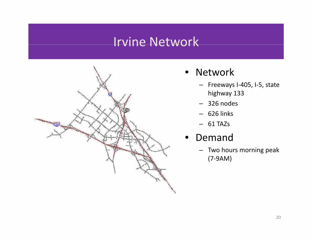
Irvine Network
• Network
Irvine Network
Network– Freeways I‐405, I‐5, state
highway 133
– 326 nodes326 nodes
– 626 links
– 61 TAZs
• Demand• Demand– Two hours morning peak
(7‐9AM)
20

Path Travel Time and Standard Deviation
• Each data point represents the mean and standard
Path Travel Time and Standard Deviation
Each data point represents the mean and standard deviation of travel times for all the vehicles (over the entire planning horizon) traveling on one path.
• Only paths with more than 10 vehicles are considered
14
8
10
12
14
Deviation
0
2
4
6
Stan
dard
0 5 10 15 20 25
Path Travel Time (minute)
21
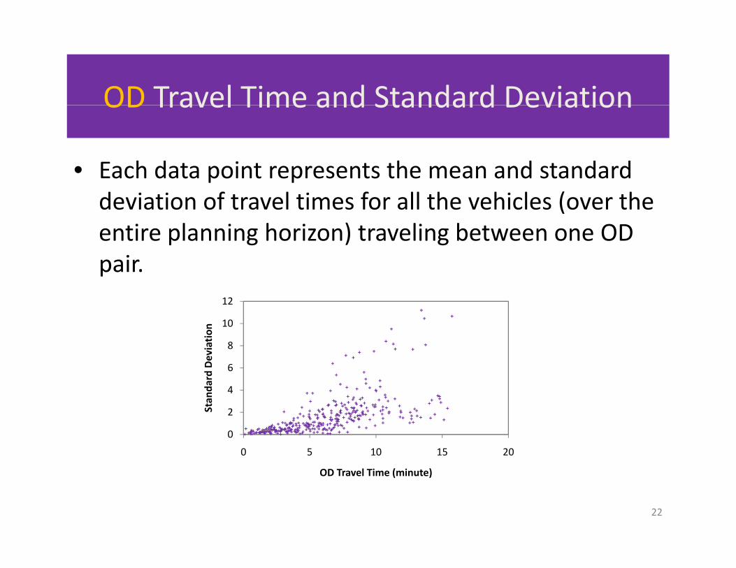
OD Travel Time and Standard Deviation
• Each data point represents the mean and standard
OD Travel Time and Standard Deviation
Each data point represents the mean and standard deviation of travel times for all the vehicles (over the entire planning horizon) traveling between one OD pair.
10
12
4
6
8
10
dard Deviation
0
2
4
0 5 10 15 20
Stan
OD Travel Time (minute)
22

Network Travel Time per Unit Distance and d d ( l)
• Each data point represents the mean and standard
Standard Deviation (5 minute interval)
Each data point represents the mean and standard deviation of travel times per mile for all vehicles departing in 5‐minute interval.
• 24 data points for 2‐hour demand
1.82
0 60.81
1.21.41.6
dard Deviation
00.20.40.6
1 1.2 1.4 1.6 1.8 2
Stan
Network Travel Time per Distance (minute/mile)
23

Network Travel Time per Distance and d d ( l)
• Each data point represents the mean and standard
Standard Deviation (1 minute interval)
Each data point represents the mean and standard deviation of travel times per mile for all vehicles departing in 1‐minute interval.
• 120 data points for 2‐hour demand
1.82
0 60.81
1.21.41.6
dard Deviation
00.20.40.6
1 1.2 1.4 1.6 1.8 2
Stan
Network Travel Time per Distance (minute/mile)
24

Network Travel Time per Distance withl h l
• Each data point represents the mean and standard
Sampling Vehicles
Each data point represents the mean and standard deviation of travel times per mile for all vehicles departing in 1‐minute interval.
• 120 data points for 2‐hour demand
1 82
0.81
1.21.41.61.8
ard Deviation
100% Sample
10% Sample
00.20.40.6
1 1.2 1.4 1.6 1.8 2
Stan
d
Network Travel Time per Distance (minute/mile)
25

CHART Network
• Network
CHART Network
Network– I‐95 corridor between
Washington, DC and Baltimore, MD, US
– 2241 nodes
– 3459 links
– 111 TAZ zones
• Demand– Two hours morning peak
(7 9AM)(7‐9AM)
26

OD Travel Time per Unit Distance and d d
• Each data point represents the mean and standard
Standard Deviation
Each data point represents the mean and standard deviation of travel times per mile for all the vehicles (over the entire planning horizon) traveling between one OD pair.
6
3
4
5
ard Deviation
0
1
2
0 2 4 6 8 10
Stan
da
0 2 4 6 8 10
OD Travel Time per Distance (minute/mile)
27

Network Travel Time per Unit Distance h l h l
• Each data point represents the mean and standard
with Sampling Vehicles
Each data point represents the mean and standard deviation of travel times per mile for all vehicles departing in 5‐minute interval.
• 24 data points for 2‐hour demand
1 82
0 81
1.21.41.61.8
ard Deviation
100% Sample
00.20.40.60.8
1 1 2 1 4 1 6 1 8 2
Stan
da
100% Sample
10% sample
1 1.2 1.4 1.6 1.8 2
Network Travel Time per Distance (minute/mile)
28
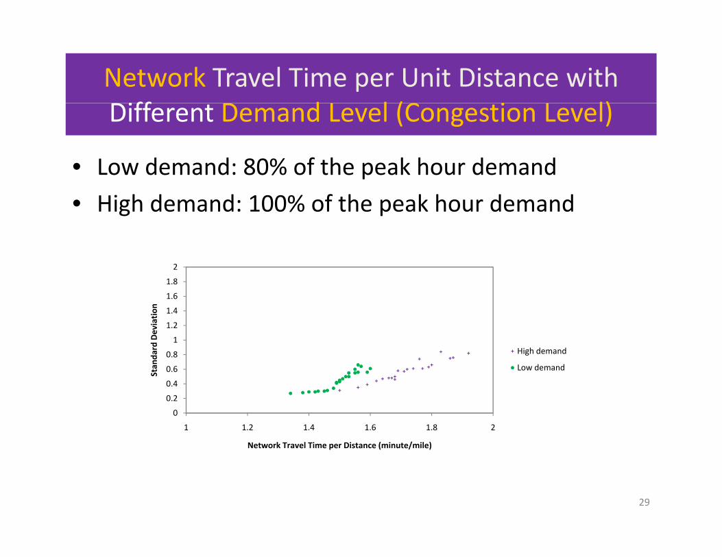
Network Travel Time per Unit Distance with iff d l (C i l)
• Low demand: 80% of the peak hour demand
Different Demand Level (Congestion Level)
Low demand: 80% of the peak hour demand
• High demand: 100% of the peak hour demand
1.4
1.6
1.8
2
on
0 4
0.6
0.8
1
1.2
Stan
dard Deviati
High demand
Low demand
0
0.2
0.4
1 1.2 1.4 1.6 1.8 2
Network Travel Time per Distance (minute/mile)
29

Network Travel Time per Unit Distance h ff k
• The mean travel time per mile range is comparable,
with Different Networks
The mean travel time per mile range is comparable, which indicates similar congestion level
• CHART network shows lower variation in travel times
1 4
1.6
1.8
2
n
0.6
0.8
1
1.2
1.4
Stan
dard Deviatio
CHART
Irvine
0
0.2
0.4
1 1.1 1.2 1.3 1.4 1.5 1.6 1.7 1.8 1.9 2
Network Travel Time per Distance (minute/mile)p ( / )
30

Concluding CommentsConcluding Comments
• Many things could be done in the short termMany things could be done in the short term to reflect reliability considerations; robust relation between SD and Mean of trip timerelation between SD and Mean of trip time PER MILE
• DTA plus robust analytical relations on supply• DTA plus robust analytical relations on supply side, w. Vovsha’s approaches to utility valuation provide low hanging fruitvaluation provide low hanging fruit
31

Concluding CommentsConcluding Comments
• Required: a more fundamental perspective on project and system evaluation that recognizes:
• Traffic physics and role of system management:• Traffic physics and role of system management: controllability and opportunities for intervention
• Short and long term dynamics of user judgment and behaviorbehavior
• Network spatial and temporal dynamics• Relevance of “external” events (accidents, weather) to evaluation frame of referenceevaluation frame of reference
• Connection between individual attitudes towards risk and social preferences
32
Related Documents