Concepts and algorithms of mapping grid-based workflow to ...

1. Dang Minh Quan School of Information Technology, International University in Germany Campus 3, 76646 Bruchsal, Germany Tel: +49 7251 700 231 Fax: +49 7251 700 250 Email: [email protected]

2. Odej Kao Electrical Engineering and Computer Science, Technical University Berlin Einsteinufer 17, 10587 Berlin, Germany Tel: +49 30 314 24230 Fax: +49 30 314 21060 Email: [email protected]

3. Jörn Altmann School of Information Technology, International University in Germany Campus 3, 76646 Bruchsal, Germany Tel: +49 7251 700 130 Fax: +49 7251 700 250 Email: [email protected]

Dang Minh Quan is senior researcher at the School of Information Technology at the International University in Bruchsal. He received his Ph.D. (2006) from the University of Paderborn, Germany. His current research centers on computer network, High Performance Computing and Grid computing. In particular, he put special focus on supporting management of SLA-based workflows in the Grid.

Odej Kao is full professor at the Berlin University of Technology (TU Berlin)

and director of the IT center tubIT. He received his PhD and his habilitation from the Clausthal University of Technology. Thereafter, he moved to the University of Paderborn as an associated professor for operating and distributed systems. His research areas include Grid Computing, context-aware systems, service level agreements and operation of complex IT systems. Odej Kao is member of many program committees and editorial boards and has published more than 150 papers.

Jörn Altmann is Associate Professor at the International University of

Bruchsal, Germany, where he heads the group of Computer Networks and Distributed Systems. He received his Ph.D. (1996) from the University of Erlangen-Nürnberg, Germany. His current research centers on the economics of Internet services and Internet infrastructures, and integrating economic models into distributed systems. In particular, he focuses on capacity planning, network topologies, and resource allocation.

Chapter # Concepts and algorithms of mapping Grid-based workflow to resources within an SLA context Dang Minh Quan, Odej Kao, Jörn Altmann Abstract: With the popularity of Grid-based workflow, ensuring the Quality of Service (QoS) for workflow by Service Level Agreements (SLAs) is an emerging trend in the business Grid. Among many system components for supporting SLA-aware Grid-based workflow, the SLA mapping mechanism is allotted an important position as it is responsible for assigning sub-jobs of the workflow to Grid resources in a way that meets the user's deadline and minimizes costs. With many different kinds of sub-jobs and resources, the process of mapping a Grid-based workflow within an SLA context defines an unfamiliar and difficult problem. To solve this problem, this chapter describes related concepts and mapping algorithms. Keywords: Grid computing, Grid-based workflow, mapping, Service Level Agreement 1. INTRODUCTION Grid computing is viewed as the next phase of distributed computing. Built on

Internet standards, it enables organizations to share computing and information

resources across departments and organizational boundaries in a secure and highly

efficient manner.

Many Grid users have a high demand of computing power to solve large scale

problems such as material structure simulation, weather forecasting, fluid dynamic

simulation, etc. Alongside a vast number of single-program applications, which has

only one sequential or parallel program, there exist many applications requiring the

co-process of many programs following a strict processing order. Since those

applications are executed on the Grid, they are called Grid-based workflows.

Traditionally, to run the application, scientific users submit it to a Grid system and the

system tries to execute it as soon as possible (Deelman et al, 2004). However, that

best-effort mechanism is not suitable when users are industry corporations, such as

BMW or Volvo which want run dynamic fluid simulation to help produce cars. These

users need a continually concurrent result at a specific time, hence requiring that the

application must be run during a specific period. Because they are commercial users,

they are willing to pay for the results to be on time. This requirement must be agreed

on by both users and the Grid system before the application is executed and can be

done legally by a Service Level Agreement (SLA) because its purpose is to identify

the shared goals and objectives of the concerned parties.

A good SLA is important as it sets boundaries and expectations for the subsequent

aspects of a service provision. An SLA clearly defines what the user wants and what

the provider promises to supply, helping to reduce the chances of disappointing the

customer. The provider's promises also help the system stay focused on customer

requirements and assure that the internal processes move in the proper direction. As

an SLA describes a clear, measurable standard of performance, internal objectives

become clear, measurable, and quantifiable. An SLA also defines penalties, thereby

allowing the customer to understand that the service provider truly believes in its

ability to achieve the performance levels set. It makes the relationship clear and

positive, establishes the expectations between the consumer and the provider, and

defines their relationship.

One of the core problems in running a Grid-based workflow within an SLA context is

how to map sub-jobs of the workflow to Grid resources. An automated mapping is

necessary as it frees users from the tedious job of assigning sub-jobs to resources

under many constraints such as workflow integrity, on time conditions, optimal

conditions and so on. Additionally, a good mapping mechanism will help users save

money and increase the efficiency of using Grid resources. In particular, the SLA

context requires that the mapping mechanism must satisfy two main criteria.

- The algorithm must ensure finishing the workflow execution on time. This

criterion is quite clear because it is the main reason for an SLA system to exist.

The criterion imposes that the underlying Grid infrastructure must be High

Performance Computing Centers and the resources must be reserved.

- The algorithm must optimize the running cost. This criterion is derived from the

business aspect of an SLA. If a customer wants to use a service, he must pay for it

and therefore has the right to an appropriate quality.

The workflow, the resource configurations, and the goal influenced by the SLA

context define a complicated mapping problem. This chapter will present related

concepts and a mechanism, which includes several sub optimization algorithms, to

map sub-jobs of the workflow to the Grid resources within an SLA context, thus

satisfying the specific user's runtime requirement and optimizing the cost. At present,

the size of the Grid is still small. For example, the Distributed European Infrastructure

for Supercomputing Applications (DEISA) includes only 11 sites. Based on that, a

distributed mapping model for very large size Grid is not an urgent requirement at

present and thus not focused on. The goal of this work is to provide a fast and

effective response solution while ensuring the QoS for customers, reducing the

overhead of the workflow execution time and encouraging the utilization of the

services.

The chapter is organized as follows. Section 2 describes the related concepts. Section

3 presents the problem statement and Section 4 describes the algorithm. Section 5

describes the performance evaluation and section 6 concludes with a short summary.

2. BASIC CONCEPTS 2.1. Service Level Agreement The main purpose of an Information Technology organization is to provide a

computing service which satisfies the customers' business requirements. To achieve

this, the organization needs to understand those requirements and to evaluate its own

capability of providing the service and of measuring the service delivered. To realize

this process, the service and level of delivery required must be identified and agreed

between the organization and its users. This is usually done by Service Level

Agreements (SLAs), which are contracts developed jointly by the organization and

the customers.

An SLA identifies the agreed upon services to be provided to a customer so as to

ensure that they meet the customer's requirements. It identifies customers'

expectations and defines the boundaries of the service, stating agreed-upon service

level goals, operating practices, and reporting policies. Webopedia defines an SLA as

" a contract between an ASP (Application Service Provider) and the end user which

stipulates and commits the ASP to a required level of service. An SLA should contain

a specified level of service, support options, enforcement or penalty provisions for

services not provided, a guaranteed level of system performance as relates to

downtime or uptime, a specified level of customer support and what software or

hardware will be provided and for what fee."

A common SLA contains the following components:

- Parties joining the agreement which is made between the service provider and the

service user. The two participants should exist as individuals, either by name or by

title and both sides must sign the document.

- Type and the time window of the service to be provided. The SLA must state

clearly which service will be provided and the time window during which the

service is provided to the user. In fact, there are a lot of system components

contributing to the type definition of the service. They can be the number of

processors, processor speed, amount of memory, communication library, and so

forth.

- The guaranty of the provider to provide the appropriate service and performance.

The SLA must state clearly how well the service will be provided to the user as

Quality of Service. Penalties must also be figured out if a certain QoS cannot be

satisfied.

- The cost of the service. Business users wishing to use any service have to pay for

it with the cost depending on the quantity of service usage and how long the user

uses it.

- The measurement method and reporting mechanism. The SLA defines which

parameters will be measured and the method of measuring. Data collected from

the monitoring procedure are important as they help both the user and provider

check the validity of the SLA.

2.2 Grid-based workflow Workflows received enormous attention in the databases and information systems

research and development community (Georgakopoulos et al, 1995). According to the

definition from the Workflow Management Coalition (WfMC) (Fischer, 2004), a

workflow is "The automation of a business process, in whole or parts, where

documents, information or tasks are passed from one participant to another to be

processed, according to a set of procedural rules." Although business workflows

have great influence on research and development, another class of workflows

emerges naturally in sophisticated scientific problem-solving environments called

Grid-based workflow. A Grid-based workflow differs slightly from the WfMC

definition as it concentrates on intensive computation and data analyzing but not on

the business process. A Grid-based workflow is characterized by following features

(Singh and Vouk, 1997).

- A Grid-based workflow usually includes many applications which perform data

analysis tasks. However, those applications, which are also called sub-jobs, are

not executed freely but in a strict sequence.

- A sub-job in the Grid-based workflow depends tightly on the output data from the

previous sub-job. With incorrect input data, the sub-job will produce a wrong

result and damage the result of the whole workflow.

- Sub-jobs in the Grid-based workflow are usually computationally intensive tasks,

which can be sequential or parallel programs and require long runtime.

- Grid-based workflows usually require powerful computing facilities such as super

computers or cluster on which to run.

Obviously, that the Grid-based workflow and the business workflow have the same

primary characteristic as they both have a procedure that applies a specific

computation into selected data based on certain rules. Each Grid-based workflow is

defined by three main factors.

- Tasks. A task in the Grid-based workflow is a sub-job, i.e., a specific program

doing a specific function. Within a Grid-based workflow, a sub-job can be a

sequential program or a parallel program and usually has a long running period

and needs powerful computing resources. Each sub-job requires specific resources

for the running process such as operating system (OS), amount of storage, CPU,

memory, etc.

- Control aspect. The control aspect describes the structure and the sequence in

processing of sub-jobs in the workflow.

- Information aspect. The information aspect of the Grid-based workflow is

presented by data transmissions. The dependency among sub-jobs can also be

identified by the data transmission task. A sub-job is executed to produce a

number of output data, which become the input data for the next sub-job in the

sequence. These data must be transferred to the place where the next sub-job is

executed. Within a Grid-based workflow, the quantity of data to be transferred

between two sub-jobs varies from several KB to a hundred GB depending on the

type of application and its scope.

Most of existing Grid-based workflows (Ludtke et al, 1999, Berriman et al, 2003,

Lovas et al, 2004) can be presented under Directed Acyclic Graph (DAG) form so

only the DAG workflow is considered in this chapter. Figure 1 presents a sample of a

workflow as a material for presentation.

Subjob 0

Subjob 5

Subjob 4

Subjob 3

Subjob 6Subjob 2Subjob 18 7

7

5 3

2

2

3

9

2

Figure 1: A sample Grid-based workflow The user specifies the required resources needed to run each sub-job, the data transfer

between sub-jobs, the estimated runtime of sub-jobs, and the expected runtime of the

entire workflow. In more detail, we will look at a concrete example, a simple Grid

workflow as presented in Figure 1. The main requirement of this workflow is

described as follows:

- Each sub-job having different resource requirements of hardware and software

configurations. Important parameters such as the number of CPUs, the size of

storage, the number of experts, and the estimated runtime for each sub-job in the

workflow are described in Table 1.

- The number above each edge describes the number of data to be transferred

between sub-jobs.

Table 1: Sub-jobs' resource requirements of the workflow in Figure 1

Sj_ID CPU Storage exp runtime 0 51 59 1 21 1 62 130 3 45 2 78 142 4 13 3 128 113 4 34 4 125 174 2 21 5 104 97 3 42 6 45 118 1 55

There are two types of resources in the resource requirements of a sub-job: adjustable

and nonadjustable. The nonadjustable resources are the type of RMS, OS, and

communication library. If a sub-job requires a supercomputer it cannot run on a

cluster. If a sub-job requires Linux OS it cannot run on Windows OS. Other types of

resources are adjustable. For example, a sub-job which requires a system with CPU

1Ghz can run on the system with CPU 2 Ghz; a sub-job requiring a system with 2GB

RAM can run on the system with 4GB RAM. Commonly, all sub-jobs in a workflow

have the same nonadjustable resources and different adjustable resources.

The distinguishing characteristic of the workflow description within an SLA context

lies in the time factor. Each sub-job must have its estimated runtime correlative with

the specific resource configuration on which to run. Thus, the sub-job can be run on

dedicated resources within a reserved time frame to ensure the QoS (this is the

runtime period). The practical Grid workload usually has a fixed input data pattern.

For example, the weather forecasting workflow is executed day by day and finishes

within a constant period of time since all data has been collected (Lovas et al, 2004).

This characteristic is the basis for estimating the Grid workload's runtime (Spooner et

al, 2003), and the runtime period of a sub-job can be estimated from statistical data.

The user usually runs a sub-job many times with different resource configurations and

different amount of input data before integrating it to the workflow. The data from

these running is a dependable source for estimating future runtimes. If these

parameters exceed the pre-determined limitation, the SLA will be violated. Within the

SLA context, the resources are reserved over time. If a sub-job runs out of an

estimated time period, it will occupy the resource of another reserved sub-job, a

situation which is not permitted in an SLA system.

The time is computed in slots with each slot equaling a specific period of real time,

from 3 to 5 minutes. We use the slot concept because we do not want to have arbitrary

start and stop time of a sub-job. Moreover, a delay of 3 minutes also has little

significance for the customer. It is noted that a sub-job of the workflow can be either a

sequential program or a parallel program and that the data to be transferred among

sub-jobs can be very large.

2.3 Grid resource The computational Grid includes many High Performance Computing Centers

(HPCCs). Sub-jobs of the workflow will be executed in HPCCs as it brings many

important advantages:

- Only these HPCCs can handle the high computing demand of scientific

applications.

- The cluster or super computer in an HPCC is relatively stable and well

maintained. This is an important feature so as to ensure finishing the sub-job

within a specific period of time.

- The HPCCs usually connect to the worldwide network by high speed links, whose

broad bandwidth makes the data transfer among sub-jobs easier and faster.

The resources of each HPCC are managed by a software called local Resource

Management System (RMS). In this chapter, RMS is used to represent the

cluster/super computer as well as the Grid services provided by the HPCC. Each RMS

has its own unique resource configuration, with difference including the number of

CPUs, amount of memory, storage capacity, software, expert, service price. To ensure

that the sub-job can be executed within a dedicated time period, the RMS must

support advance resource reservation such as CCS (Hovestadt 2003). Figure 2 depicts

a sample CPU reservation profile in such an RMS. In our system, we reserve three

main types of resource: CPUs, storages and experts. An extension to other resources

is straightforward.

Number CPU available

1728

Number CPUrequire

0 21 67 82

5145

166

435419357

138

time

Figure 2: A sample CPU reservation profile of a local RMS

10MB/sBandwidth

0 21 50 65 138

time

100 Figure 3: A sample bandwidth reservation profile of a link between two local RMSs

For present purposes, suppose that we have three involved RMSs executing the sub-

jobs of the workflow. The reservation information of the resources is presented in

Table 2. Each RMS represented by an ID_hpc value has a different number of free

CPUs, storage, and expert during a specified period of time. The sample resource

reservation profiles of the RMSs are empty.

Table 2: RMSs resource reservation ID ID_hpc CPUs storage Exp start End 31 2 128 256000 8 0 1000000 23 0 128 256000 9 0 1000000 30 1 128 256000 6 0 1000000 If two output-input-dependent sub-jobs are executed under the same RMS, it is

assumed that the time used for the data transfer equals zero, and assumption can be

made since all compute nodes in a cluster usually use a shared storage system like

NFS or DFS. In all other cases, it is assumed that a specific amount of data will be

transferred within a specific period of time, thus requiring the reservation of

bandwidth.

The link capacity between two local RMSs is determined as the average capacity

between two sites in the network, which has a different value with each different

RMS couple. Whenever a data transfer task is on a link, the available period on the

link will be determined. During that specified period, the task can use the whole

bandwidth, and other tasks must wait. Using this principle, the bandwidth reservation

profile of a link will look similar to the one depicted in Figure 3. A more precise

model with bandwidth estimation (Wolski, 2003) can be used to determine the

bandwidth within a specific time period instead of the average value. In both cases,

the main mechanism remains unchanged.

3. FORMAL PROBLEM STATEMENT

The formal specification of the described problem includes the following elements:

- Let R be the set of Grid RMSs. This set includes a finite number of RMSs, which

provide static information about controlled resources and the current

reservations/assignments.

- Let S be the set of sub-jobs in a given workflow including all sub-jobs with the

current resource and deadline requirements.

- Let E be the set of edges in the workflow, which express the dependency between

the sub-jobs and the necessity for data transfers between the sub-jobs.

- Let Ki be the set of resource candidates of sub-job si. This set includes all RMSs,

which can run sub-job si, Ki ⊂ R.

Based on the given input, a feasible and possibly optimal solution is sought, allowing

the most efficient mapping of the workflow in a Grid environment with respect to the

given global deadline. The required solution is a set defined in Formula 1.

M = {( si, rj, start_slot) | si ∈ S, rj ∈ Ki } (1)

If the solution does not have start_slot for each si, it becomes a configuration as

defined in Formula 2.

a = {( si, rj) | si ∈ S, rj ∈ Ki } (2)

A feasible solution must satisfy following conditions:

- Criterion 1: The finished time of the workflow must be smaller or equal to the

expected deadline of the user.

- Criterion 2: All Ki ≠∅. There is at least one RMS in the candidate set of each

sub-job.

- Criterion 3: The dependencies of the sub-jobs are resolved and the execution

order remains unchanged.

- Criterion 4: The capacity of an RMS must equal or be greater than the

requirement at any time slot. Each RMS provides a profile of currently available

resources and can run many sub-jobs of a single flow both sequentially and in

parallel. Those sub-jobs which run on the same RMS form a profile of resource

requirement. With each RMS rj running sub-jobs of the Grid workflow, and with

each time slot in the profile of available resources and profile of resource

requirements, the number of available resources must be larger than the resource

requirement.

- Criterion 5: The data transmission task eki from sub-job sk to sub-job si must take

place in dedicated time slots on the link between the RMS running sub-job sk to

the RMS running sub-job si. eki ∈ E.

In the next phase, the feasible solution with the lowest cost is sought. The cost C of

running a Grid workflow is defined in Formula 3. It is the sum of four factors: the cost

of using the CPU, the cost of using the storage, the cost of using the experts’

knowledge, and finally the expense for transferring data between the resources

involved.

C=�=

n

i 1

si.rt*( si.nc*rj.pc+si.ns*rj.ps+si.ne*rj.pe) + � eki.nd*rj.pd (3)

with si.rt, si.nc, si.ns, si.ne being the runtime, the number of CPUs, the number of

storage, and the number of expert of sub-job si respectively. rj.pc, rj.ps, rj.pe, rj.pd are

the price of using the CPU, the storage, the expert, and the data transmission of RMS

rj respectively. eki.nd is the number of data to be transferred from sub-job sk to sub-job

si.

If two dependent sub-jobs run on the same RMS, the cost of transferring data from the

previous sub-job to the later sub-job is neglected.

The ability to find a good solution depends mainly on the resource state at the

expected period when the workflow runs. During that period, if the number of free

resources in the profile is large, there are a lot of feasible solutions and we can choose

the cheapest one. But if the number of free resources in the profile is small, simply

finding out a feasible solution is difficult. Thus, a good mapping mechanism should

be able to find out an inexpensive solution when there is a wealth of free resources

and to be able to uncover a feasible solution when there are few free resources in the

Grid.

Supposing the Grid system has m RMSs, which can satisfy the requirement of n sub-

jobs in a workflow. As an RMS can run several sub-jobs at a time, finding out the

optimal solution needs mn loops. It can easily be shown that the optimal mapping of

the workflow to the Grid RMS as described above is an NP hard problem.

From the above description, though, we can see that this is a scheduling problem and

that it has many distinguished characteristics.

- An RMS can handle many sub-jobs of the workflow simultaneously. The RMS

supports resource reservation.

- A sub-job is a parallel application.

- The destination of the problem is optimizing the cost. The user imposes some

strict requirements on the Grid system and pays for the appropriately received

service. It is obvious that the user prefers top service at the lowest possible cost.

The expense of running a workflow includes the cost of using computation

resources and the cost of transferring data among sub-jobs.

Many other previous works (Deelman et al, 2004, Lovas et al, 2004) have the same

Grid-based workflow model as we have. But there are no resource reservations and

the goal is to optimize the runtime. Some works about supporting QoS for the Grid-

based workflows such as (McGough et al, 2005, Zeng et al, 2004, Brandic et al, 2005)

use resource reservation infrastructure and have the goal of optimizing the cost.

However, they assume a workflow with many sub-jobs, which are sequential

programs, and a Grid resource service handling one sub-job at a time. Other related

works such as the job shop scheduling problem (JSSP), and the multiprocessor

scheduling precedence-constrained task graph problem have similar context with

(McGough et al, 2005, Zeng et al, 2004, Brandic et al, 2005) but without resource

reservation. Moreover, they aim at optimizing the runtime. All above works depend

tightly on the characteristics of workload, resource and goal. Thus, adapting them to

our problem faces many difficulties concerning poor quality, long runtime or

inapplicable (Quan, 2006).

As no previous work has a similar context, we describe here a strategy to handle the

requirements. An efficient mapping mechanism will satisfy those preferences and also

increase the efficiency of using Grid resources.

4. ALGORITHMS The mapping mechanism includes three sub-algorithms. The L-Map algorithm finds

the cost optimal mapping solution for a light workflow in which the amount of data to

be transferred among sub-jobs is not much (L stands for light). The H-Map algorithm

finds the cost optimal mapping solution for heavy workflows in which the amount of

data to be transferred among sub-jobs is large (H stands for heavy). The w-Tabu

algorithm finds the runtime optimal solution for both cases of workflows (w stands

for workflow).

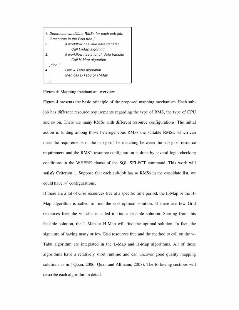
1. Determine candidate RMSs for each sub-job. If resource in the Grid free {2. if workflow has little data transfer

Call L-Map algorithm3. if workflow has a lot of data transfer

Call H-Map algorithm }else {4. Call w-Tabu algorithm

then call L-Tabu or H-Map }

Figure 4: Mapping mechanism overview Figure 4 presents the basic principle of the proposed mapping mechanism. Each sub-

job has different resource requirements regarding the type of RMS, the type of CPU

and so on. There are many RMSs with different resource configurations. The initial

action is finding among those heterogeneous RMSs the suitable RMSs, which can

meet the requirements of the sub-job. The matching between the sub-job's resource

requirement and the RMS's resource configuration is done by several logic checking

conditions in the WHERE clause of the SQL SELECT command. This work will

satisfy Criterion 1. Suppose that each sub-job has m RMSs in the candidate list, we

could have mn configurations.

If there are a lot of Grid resources free at a specific time period, the L-Map or the H-

Map algorithm is called to find the cost-optimal solution. If there are few Grid

resources free, the w-Tabu is called to find a feasible solution. Starting from this

feasible solution, the L-Map or H-Map will find the optimal solution. In fact, the

signature of having many or few Grid resources free and the method to call on the w-

Tabu algorithm are integrated in the L-Map and H-Map algorithms. All of those

algorithms have a relatively short runtime and can uncover good quality mapping

solutions as in ( Quan, 2006, Quan and Altmann, 2007). The following sections will

describe each algorithm in detail.

4.1 w-Tabu algorithm The main purpose of the w-Tabu algorithm is to find out a feasible solution when

there are few free Grid resources. This destination is equal to finding a solution with

the minimal finished time. Within the SLA context as defined in section 2, the

finished time of the workflow depends on the reservation state of the resources in the

RMSs, the bandwidth among RMSs, and the bandwidth reservation state. It is easy to

show that this task is an NP hard problem. Although the problem has the same

destination as most of the existing algorithm mapping a DAG to resources (Deelman

et al, 2004), the defined context is different from all other contexts appearing in the

literature. Thus, a dedicated algorithm is necessary. We proposed a mapping strategy

as depicted in Figure 5. This algorithm has proven to be better than the application of

Min-min, Max-min, Suffer, GRASP, w-DCP to the problem as described in (Quan,

2006).

WorkflowsDAG

RMSs

Construct setof referenceconfiguration

CoImprove the

quality ofconfigurations

Output thebest

configuration

Figure 5: w-Tabu algorithm overview Firstly, a set of referent configurations is created. Then we use a specific module to

improve the quality of each configuration as much as possible with the best

configuration being selected. This strategy looks similar to an abstract of a long term

local search such as Tabu search, Grasp, SA and so on. However, a detailed

description makes our algorithm distinguishable from them.

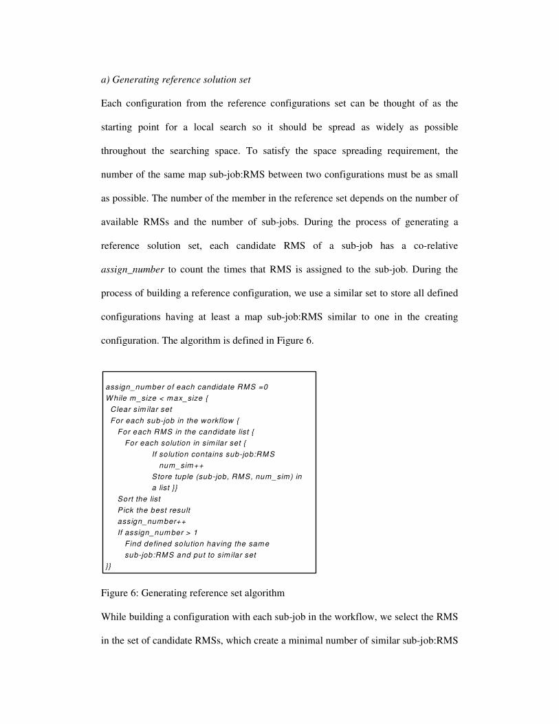
a) Generating reference solution set Each configuration from the reference configurations set can be thought of as the

starting point for a local search so it should be spread as widely as possible

throughout the searching space. To satisfy the space spreading requirement, the

number of the same map sub-job:RMS between two configurations must be as small

as possible. The number of the member in the reference set depends on the number of

available RMSs and the number of sub-jobs. During the process of generating a

reference solution set, each candidate RMS of a sub-job has a co-relative

assign_number to count the times that RMS is assigned to the sub-job. During the

process of building a reference configuration, we use a similar set to store all defined

configurations having at least a map sub-job:RMS similar to one in the creating

configuration. The algorithm is defined in Figure 6.

assign_number of each candidate RMS =0W hile m _size < max_size { Clear sim ilar set For each sub-job in the workflow { For each RMS in the candidate list { For each solution in sim ilar set {

If solution contains sub-job:RMS num_sim++Store tuple (sub-job, RMS, num_sim) ina list }}

Sort the list Pick the best result assign_number++ If assign_num ber > 1 Find defined solution having the same sub-job:RMS and put to sim ilar set}}

Figure 6: Generating reference set algorithm While building a configuration with each sub-job in the workflow, we select the RMS

in the set of candidate RMSs, which create a minimal number of similar sub-job:RMS

with other configurations in the similar set. After that, we increase the assign_number

of the selected RMS. If this value is larger than 1, meaning that the RMS were

assigned to the sub-job more than one time, there must exist configurations that

contain the same sub-job:RMS and thus satisfy the similar condition. We search these

configurations in the reference set which have not been in the similar set, and then add

them to the similar set. When finished, the configuration is put to the reference set.

After all reference configurations have been defined, we use a specific procedure to

refine each of the configuration as much as possible.

b) Solution improvement algorithm To improve the quality of a configuration, for this problem we use a specific

procedure based on short term Tabu search. We use Tabu Search because it can also

play the role of a local search but with a wider search area. Besides the standard

components of Tabu Search, there are some components specific to the workflow

problems.

The neighborhood set structure

One of the most important concepts of Tabu Search as well as local search is the

neighborhood set structure. A configuration can also be presented as a vector. The

index of the vector represents the sub-job, and the value of the element represents the

RMS. With a configuration a, a=a1a2. . .an | with all ai ⊂ Ki, we generate n*(m-1)

configurations a' as in Figure \ref{fig436}. We change the value of xi to each and

every value in the candidate list which is different from the present value. Each

change results in a new configuration. After that we have set A, |A|=n*(m-1). A is the

set of neighborhoods of a configuration. A detailed neighborhood set for the case of

our example is presented in Figure 7.

a

m-1

m-1

m-1

na2a1x

na2x1a

nx2a1a

Where ix

and ix != ia

in [1,n]

Figure 7: Neighborhood structure of a configuration

1 32121 3

{2,3} {2,3} {1,3} {2,3} {1,3} {1,2} {1,2}

Figure 8: Sample neighborhood structure of a configuration

The assigning sequence of the workflow

When the RMS executed each sub-job, the bandwidth among sub-jobs was

determined, the next task is to locate a time slot to run sub-job in the specified RMS.

At this point, the assigning sequence of the workflow becomes important. The

sequence of determining runtime for sub-jobs of the workflow in an RMS can also

affect the final finished time of the workflow, especially when there are many sub-

jobs in the same RMS.

In general, to ensure the integrity of the workflow, sub-jobs in the workflow are

assigned based on the sequence of the data processing. However, that principal does

not cover the case of a set of sub-jobs, which have the same priority in data sequence

and do not depend on each other. To examine the problem, we determine the earliest

and the latest start time of each sub-jobs of the workflow under an ideal condition.

The time period for data transfer among sub-jobs is computed by dividing the amount

of data to a fixed bandwidth. The earliest and latest start and stop time for each sub-

job and data transfer depends only on the workflow topology and the runtime of sub-

jobs but not the resources context. These parameters can be determined using

conventional graph algorithms. A sample of these data for the workflow in Figure 1,

in which the number above each link represents the number of time slots for data

transfer, is presented in Table 3.

Table 3: Valid start time for sub-jobs of workflow in Figure 1 Sub-job Earliest start Latest start 0 0 0 1 28 28 2 78 78 3 28 58 4 30 71 5 23 49 6 94 94 The ability of finding a suitable resource slot to run a sub-job depends on the number

of resources free during the valid running period. From the graph, we can see sub-job

1 and sub-job 3 as having the same priority in the data sequence. However, sub-job 1

can start at max time slot 28 while sub-job 3 can start at max time slot 58 without

affecting the finished time of workflow. Suppose that two sub-jobs are mapped to run

in the same RMS and the RMS can run one sub-job at a time. If sub-job 3 is assigned

first and in the worst case at time slot 58, sub-job 1 will be run from time slot 92, thus

the workflow will be late a minimum of 64 time slots. If sub-job 1 is assigned first at

time slot 28, sub-job 3 can be run at time slot 73 and the workflow will be late by 15

time slots. Here we can see the latest time factor is the main parameter for evaluating

the full effect of the sequential assigning decision. It can be seen through the

affection, mapping sub-job having the smaller latest start time first will make the

lateness less. Thus, the latest start time value determined as above can be used to

determine the assigning sequence. The sub-job having the smaller latest start time will

be assigned earlier. This procedure will satisfy Criterion 3.

Computing the timetable procedure

The algorithm to compute the timetable is presented in Figure 9. As the w-Tabu

algorithm applies both for light workflow and heavy workflow, determining the

parameter for each case cannot be the same. With light workflow, the end time of the

data transfer equals the time slot after the end of the correlative source sub-job. With a

heavy workflow, the end time of data transfer is determined by searching the

bandwidth reservation profile. This procedure will satisfy Criteria 4 and 5.

With each sub-job k following the assign sequence { Determine set of assigned sub-jobs Q, which having output data transfer to the sub-job k With each sub-job i in Q { min_st_tran=end_time of sub-job i +1 If heavy weight workflow { Search in reservation profile of link between RMS running sub-job k and RMS running sub-job i to determine start and end time of data transfer task with the start time > min_st_tran } else { end time data transfer = min_st_tran } } min_st_sj=max end time of all above data transfer +1 Search in reservation profile of RMS running sub-job k to determine its start and end time with the start time > min_st_sj}

Figure 9: Determining timetable algorithm for workflow in w-Tabu

The modified Tabu Search procedure

In the normal Tabu search, in each move iteration, we will try assigning each sub-job

si ⊂ S with each RMS rj in the candidate set Ki and use the procedure in Figure 9 to

compute the runtime and then check for overall improvement and select the best one.

This method is not efficient as it requires a lot of time for computing the runtime of

the workflow which is not a simple procedure. We will improve the method by

proposing a new neighborhood with two comments.

Let C is the set of sub-jobs in the critical pathPut last sub-job into Cnext_subjob=last sub-jobdo{ prev_subjob is determined as the sub-job having latest finished data output transfer to next_subjob Put prev_subjob into C next_sj=prev_subjob} until prev_sj= first sub-job

Figure 10: Determining critical path algorithm Comment 1: The runtime of the workflow depends mainly on the execution time of

the critical path. In one iteration, we can move only one sub-job to one RMS. If the

sub-job does not belong to the critical path, after the movement, the old critical path

will have a very low probability of being shortened and the finished time of the

workflow will have a low probability of improvement. Thus, we concentrate only on

sub-jobs in the critical path. With a defined solution and runtime table, the critical

path of a workflow is defined with the algorithm in Figure 10.

We start with the last sub-job determined. The next sub-job of the critical path will

have the latest finish data transferred to the previously determined sub-job. The

process continues until the next sub-job is equal to first sub-job. Figure 11 depicts a

sample critical path of the workflow in Figure 1.

Subjob

0Subjob

1Subjob

6Subjob

2 Figure 11: Sample critical path of the workflow in Figure 1 Comment 2: In one move iteration, with only one change of one sub-job to one RMS,

if the finish time of the data transfer from this sub-job to the next sub-job in the

critical path is not decreased, the critical path cannot be shortened. For this reason, we

only consider the change which reduces the finish time of consequent data transfer. It

can easy be seen that checking if the data transfer time can be improved is much

shorter than computing the runtime table for the whole workflow.

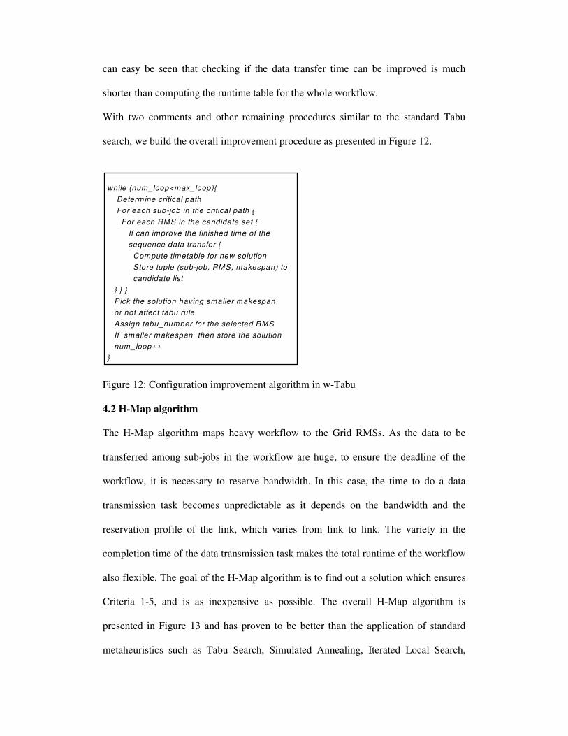
With two comments and other remaining procedures similar to the standard Tabu

search, we build the overall improvement procedure as presented in Figure 12.

while (num_loop<max_loop){ Determine critical path For each sub-job in the critical path { For each RMS in the candidate set { If can improve the finished time of the sequence data transfer { Compute timetable for new solution Store tuple (sub-job, RMS, makespan) to candidate list } } } Pick the solution having smaller makespan or not affect tabu rule Assign tabu_number for the selected RMS If smaller makespan then store the solution num_loop++}

Figure 12: Configuration improvement algorithm in w-Tabu 4.2 H-Map algorithm The H-Map algorithm maps heavy workflow to the Grid RMSs. As the data to be

transferred among sub-jobs in the workflow are huge, to ensure the deadline of the

workflow, it is necessary to reserve bandwidth. In this case, the time to do a data

transmission task becomes unpredictable as it depends on the bandwidth and the

reservation profile of the link, which varies from link to link. The variety in the

completion time of the data transmission task makes the total runtime of the workflow

also flexible. The goal of the H-Map algorithm is to find out a solution which ensures

Criteria 1-5, and is as inexpensive as possible. The overall H-Map algorithm is

presented in Figure 13 and has proven to be better than the application of standard

metaheuristics such as Tabu Search, Simulated Annealing, Iterated Local Search,

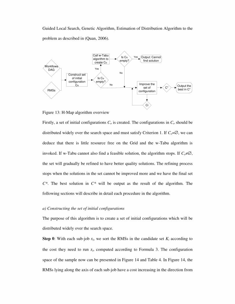
Guided Local Search, Genetic Algorithm, Estimation of Distribution Algorithm to the

problem as described in (Quan, 2006).

WorkflowsDAG

RMSs

Construct setof initial

configurationCo Improve the

set ofconfiguration

Ci

C* Output thebest in C*

Is Coempty?

No

Yes

Output: Cannotfind solution

YesCall w-Tabualgorithm tocreate Co

Is Coempty?

No

Figure 13: H-Map algorithm overview Firstly, a set of initial configurations Co is created. The configurations in Co should be

distributed widely over the search space and must satisfy Criterion 1. If Co=∅, we can

deduce that there is little resource free on the Grid and the w-Tabu algorithm is

invoked. If w-Tabu cannot also find a feasible solution, the algorithm stops. If Co≠∅,

the set will gradually be refined to have better quality solutions. The refining process

stops when the solutions in the set cannot be improved more and we have the final set

C*. The best solution in C* will be output as the result of the algorithm. The

following sections will describe in detail each procedure in the algorithm.

a) Constructing the set of initial configurations The purpose of this algorithm is to create a set of initial configurations which will be

distributed widely over the search space.

Step 0: With each sub-job si, we sort the RMSs in the candidate set Ki according to

the cost they need to run si, computed according to Formula 3. The configuration

space of the sample now can be presented in Figure 14 and Table 4. In Figure 14, the

RMSs lying along the axis of each sub-job have a cost increasing in the direction from

inside out. The line connecting each point in every sub-job axis will form a

configuration. Figure 14 presents 3 configurations with an increasing index in the

direction from inside to outside. Figure 14 also presents the cost distribution of the

configuration space according to Formula 3. The configuration in the outer layers has

a greater cost than those the inner layers. The cost of the configuration lying between

two layers is greater than the cost of the inner layer and smaller than the cost of the

outer layer.

1

3

2

1

23

2 1 33

1

2

3

2

1

231

13

2

0sj

1sj

2sj

3sj4sj

5sj

6sj 1

2

3

Figure 14: The configuration space according to cost distribution Table 4: RMSs candidate for each sub-job in cost order Sj_ID RMS RMS RMS sj0 R1 R3 R2 sj1 R1 R2 R3 sj2 R2 R1 R3 sj3 R3 R1 R2 sj4 R3 R2 R1 sj5 R2 R3 R1 sj6 R1 R3 R2 Step 1: We pick the first configuration as the first layer in the configuration space.

The determined configuration can be presented as a vector. The index of the vector

represents the sub-job, and the value of the element represents the RMS. The first

configuration in our example is presented in Figure 15. Although this has minimal

cost according to Formula 3, we cannot be sure that it is the optimal solution. The real

cost of a configuration must consider the neglected cost of data transmission when

two sequential sub-jobs are in the same RMS.

1 23321 1

0 2 4 51 63 Figure 15: The first selection configuration of the sample Step 2: We construct the other configurations by following a process similar to the

one described in Figure 16. The second solution is the second layer of the

configuration space. Then we create a solution having a cost located between layer 1

and layer 2 by combining the first and the second configurations. To do this, we take

the p first elements from the first vector configuration and then the p second elements

from the second vector configuration and repeat until we have n elements to form the

third one. Thus, we get (n/2) elements from the first vector configuration and (n/2)

other elements from the second one. Combining in this way will ensure the target

configuration of having a greater difference in cost according to Formula 3 compared

to the source configurations. This process continues until the final layer is reached.

Thus, we have in total 2*(m-1) configurations and we can ensure that the set of initial

configurations is distributed over the search space according to cost criteria.

1 23321 1

3 21123 3

3 32112 3

1 22232 1

2 11233 2

1

5

3

4

2

Figure 16: Procedure to create the set of initial configurations Step 3: We check Criteria 4 and 5 of all 2*m-1 configurations. To verify Criteria 4

and 5, we have to determine the timetable for all sub-jobs of the workflow. The

procedure to determine the timetable of the workflow is similar to the one described

in Figure 9. If some of them do not satisfy the Criteria 4 and 5 requirement, we

construct more so as to have enough 2*m-1 configurations. To do the construction, we

change the value of p parameter in the range from 1 to (n/2) in step 2 to create the

new configuration.

After this phase we have set Co including maximum (2m-1) valid configurations.

b) Improving solution quality algorithm To improve the quality of the solutions, we use the neighborhood structure as

described in Section 4.1 and Figure 7. Call A the set of neighborhood of a

configuration. The procedure to find the highest quality solution includes the

following steps.

Step 1: ∀ a ⊂ A , calculate cost(a) and timetable(a), pick a* with the smallest

cost(a*) and satisfy Criterion 2, put a* to set C1. The detailed technique of this step is

described in Figure 17.

For each subjob in the workflow { For each RMS in the candidate list { If cheaper then put (sjid, RMS id, improve_value) to a list }}Sort the list according to improve_valueFrom the begin of the list{ Compute time table to get the finished time If finished time < limit break}Store the result

Figure 17: Algorithm to improve the solution quality

We consider only the configuration having a smaller cost than the present

configuration. Therefore, instead of computing the cost and the timetable of all

configurations in the neighborhood set, we compute only the cost of them. All the

cheaper configurations are stored in a sorted list. And then we compute the timetable

of cheaper configurations along the list to find the first feasible configuration. This

technique helps to decrease much of the algorithm's runtime.

Step 2: Repeat step 1 with all a ⊂ Co to form C1.

Step 3: Repeat step 1 to 2 until Ct=Ct-1.

Step 4: Ct ≡ C*. Pick the best configuration of C*.

4.3 L-Map algorithm The key difference between the light workflow and the heavy workflow is the

communication. HPCCs are usually inter-connected by a broadband link greater than

100Mbps. The length of one time slot in our system is between 2 and 5 minutes. Thus,

the amount of data transferred through a link within one time slot can range from

1.2GB to 3GB. Since we assume less than 10MB of data transfer between sub-jobs

(workflows with light communications), the data transfer can easily be performed

within one time slot (right after the sub-job had finished its calculation) without

affecting any other communication between two RMSs. As the number of data to be

transferred between sub-jobs in the workflow is very small, we can omit the cost of

data transfer. Thus, the cost C of a Grid workflow is defined in Formula 3 which is

the sum of the charge of using: (1) the CPU, (2) the storage and (3) the expert

knowledge.

The light communication can help us ignore the complexities in time and cost caused

by data transfer. Thus, we could apply a specific technique to improve the speed and

the quality of the mapping algorithm. In this section, we present an algorithm called

L-Map to map light communication workflows onto the grid RMSs (L – stands for

light). The goal of the L-Map algorithm is to find a solution which satisfies Criterion

1-5 and is as inexpensive as possible. The overall L-Map algorithm to map DAG to

resources is presented in Figure 18. The main idea of the algorithm is to find out a

high quality and feasible solution. Starting from this solution, we limit the solution

space and use local search to find intensively in this space the best feasible solution.

This algorithm has proven to be better than the application of H-map, DBC, Genetic

Algorithm to the problem as described in (Quan and Altmann, 2007).

The following sections will describe in detail each procedure in the algorithm.

Create firstfeasiblesolution

WorkflowsDAG

RMSs

Localsearch

resultLimit the solutionspace & create set ofinitial configurations

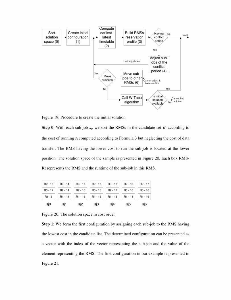
Figure 18: Framework of the L-Map algorithm a) Creating the initial feasible solution The sequence of steps in the procedure of creating the initial feasible solution is

presented in Figure 19.

Sortsolution

space (0)

Create initialconfiguration

(1)

Computeearliest-

latesttimetable

(2)

Build RMSsreservationprofile (3)

Adjust sub-jobs of the

conflictperiod (4)

Havingconflictperiod

resultNo

Yes

Had adjustment

Move sub-jobs to other

RMSs (6)Cannot adjust &

have conflict

Movesuccess

Yes

No

Call W-Tabualgorithm

Is initialsolutionavailable

Yes

NoCannot find

solution

Figure 19: Procedure to create the initial solution Step 0: With each sub-job si, we sort the RMSs in the candidate set Ki according to

the cost of running si computed according to Formula 3 but neglecting the cost of data

transfer. The RMS having the lower cost to run the sub-job is located at the lower

position. The solution space of the sample is presented in Figure 20. Each box RMS-

Rt represents the RMS and the runtime of the sub-job in this RMS.

R1-16

R3 - 17

R2 - 16

R1 - 14

R2 - 14

R3 - 14

R1 - 16

R2 - 16

R3 - 17

R1 - 16

R3 - 15

R2 - 17

sj1 sj2 sj3 sj4

R1 - 15

R2 - 17

R3 - 15

R1 - 14

R3 - 16

R2 - 16

R1 - 16

R3 - 16

R2 - 17

sj0 sj5 sj6 Figure 20: The solution space in cost order Step 1: We form the first configuration by assigning each sub-job to the RMS having

the lowest cost in the candidate list. The determined configuration can be presented as

a vector with the index of the vector representing the sub-job and the value of the

element representing the RMS. The first configuration in our example is presented in

Figure 21.

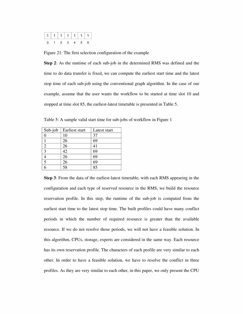
1 11111 1

0 2 4 51 63 Figure 21: The first selection configuration of the example Step 2: As the runtime of each sub-job in the determined RMS was defined and the

time to do data transfer is fixed, we can compute the earliest start time and the latest

stop time of each sub-job using the conventional graph algorithm. In the case of our

example, assume that the user wants the workflow to be started at time slot 10 and

stopped at time slot 85, the earliest-latest timetable is presented in Table 5.

Table 5: A sample valid start time for sub-jobs of workflow in Figure 1 Sub-job Earliest start Latest start 0 10 37 1 26 69 2 26 41 3 42 69 4 26 69 5 26 69 6 58 85 Step 3: From the data of the earliest-latest timetable, with each RMS appearing in the

configuration and each type of reserved resource in the RMS, we build the resource

reservation profile. In this step, the runtime of the sub-job is computed from the

earliest start time to the latest stop time. The built profiles could have many conflict

periods in which the number of required resource is greater than the available

resource. If we do not resolve those periods, we will not have a feasible solution. In

this algorithm, CPUs, storage, experts are considered in the same way. Each resource

has its own reservation profile. The characters of each profile are very similar to each

other. In order to have a feasible solution, we have to resolve the conflict in three

profiles. As they are very similar to each other, in this paper, we only present the CPU

profile to demonstrate the idea. In our example, only RMS1 appears in the

configuration. The CPU reservation profile of the RMS 1 is presented in Figure 22.

10

96

26 37 58 69 85

272

208

144

42

Time

Num CPU

Number ofavailable CPU

Figure 22: Reservation profile of RMS 1 Step 4: There are many sub-jobs joining the conflict period. If we move sub-jobs out

of it, the conflict rate will be reduced. This movement is performed by adjusting the

earliest start time or the latest stop time of the sub-jobs and thus, the sub-jobs are

moved out of the conflict period. One possible solution is shown in Figure 23 (a),

where either the latest stop time of sub-job1 is set to t1 or the earliest start time of

sub-job2 is set to t2. The second way is to adjust two sub-jobs simultaneously as

depicted in Figure 23 (b). A necessary prerequisite here is that, after adjustment, the

latest stop time minus the earliest start time of the sub-job is greater than its runtime.

rate

0 t1 t2

time

sj1sj22

rate

0 t1 t2

time

sj1sj2

rate

0 t1 t2time

sj1sj2

rate

0 t1 t2

time

sj1 sj2

a) Moving sub-jobs b) Adjusting sub-jobs Figure 23: Resolving the conflict period Step 5: We adjust the earliest start time and latest stop time of the sub-jobs relating

with the moved sub-jobs to ensure the integrity of the workflow. Then we repeat step

3 and 4 until we cannot adjust the sub-jobs further. In our example, after this phase,

the CPU reservation profile of RMS 1 is presented in Figure 24.

10

96

26 37 58 69 85

272

208

144

42

Time

Num CPU

Number ofavailable CPU

Figure 24: Reservation profile of RMS 1 after adjusting Step 6: If after the adjusting phase, there are still some conflict periods, we have to

move some sub-jobs contributing to the conflict to other RMSs. The resources in the

RMS having the conflict period should be allocated as much as possible so that the

cost for using resources will be kept to a minimum. This is a knapsack problem,

which is known to be NP-hard. Therefore, we use an algorithm as presented in Figure

25. This algorithm ensures that the remaining free resources after the filling phase is

always smaller than the smallest sub-job. If a sub-job cannot be moved to another

RMS, we can deduce that the Grid resource is busy and thus w-Tabu algorithm is

invoked. If the w-Tabu cannot find an initial feasible solution, the algorithm will stop.

Select the most serious conflict periodDetermine all sub-jobs contributing to the periodSort those sub-jobs according to cost in descend orderFor each sub-job in the list { If the resource free greater than the resource required by the sub-job Let the sub-job stay in the RMS Update the number of resource free of the period Else Assign the sub-job to the next RMS in its sorted candidate list}

Figure 25: Moving sub-jobs algorithm

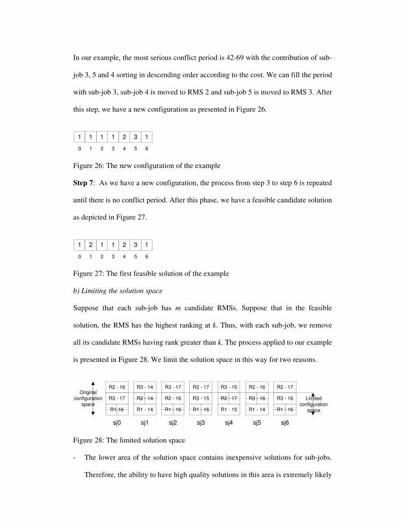
In our example, the most serious conflict period is 42-69 with the contribution of sub-

job 3, 5 and 4 sorting in descending order according to the cost. We can fill the period

with sub-job 3, sub-job 4 is moved to RMS 2 and sub-job 5 is moved to RMS 3. After

this step, we have a new configuration as presented in Figure 26.

1 32111 1

0 2 4 51 63 Figure 26: The new configuration of the example Step 7: As we have a new configuration, the process from step 3 to step 6 is repeated

until there is no conflict period. After this phase, we have a feasible candidate solution

as depicted in Figure 27.

1 32112 1

0 2 4 51 63 Figure 27: The first feasible solution of the example b) Limiting the solution space Suppose that each sub-job has m candidate RMSs. Suppose that in the feasible

solution, the RMS has the highest ranking at k. Thus, with each sub-job, we remove

all its candidate RMSs having rank greater than k. The process applied to our example

is presented in Figure 28. We limit the solution space in this way for two reasons.

R1-16

R3 - 17

R2 - 16

R1 - 14

R2 - 14

R3 - 14

R1 - 16

R2 - 16

R3 - 17

R1 - 16

R3 - 15

R2 - 17

sj1 sj2 sj3 sj4

R1 - 15

R2 - 17

R3 - 15

R1 - 14

R3 - 16

R2 - 16

R1 - 16

R3 - 16

R2 - 17

sj0 sj5 sj6

Limitedconfiguration

space

Originalconfiguration

space

Figure 28: The limited solution space - The lower area of the solution space contains inexpensive solutions for sub-jobs.

Therefore, the ability to have high quality solutions in this area is extremely likely

and should be considered intensively. In contrast, the higher area of the solution

space contains expensive solutions for sub-jobs and thus, the ability to have a high

quality solution in this area is very unlikely. For that reason, to save the

computation time, we can by pass this area.

- The selected solution space contains at least one feasible solution. Thus, we can

be sure that with this new solution space we can always uncover an equal or better

solution than the previously found one.

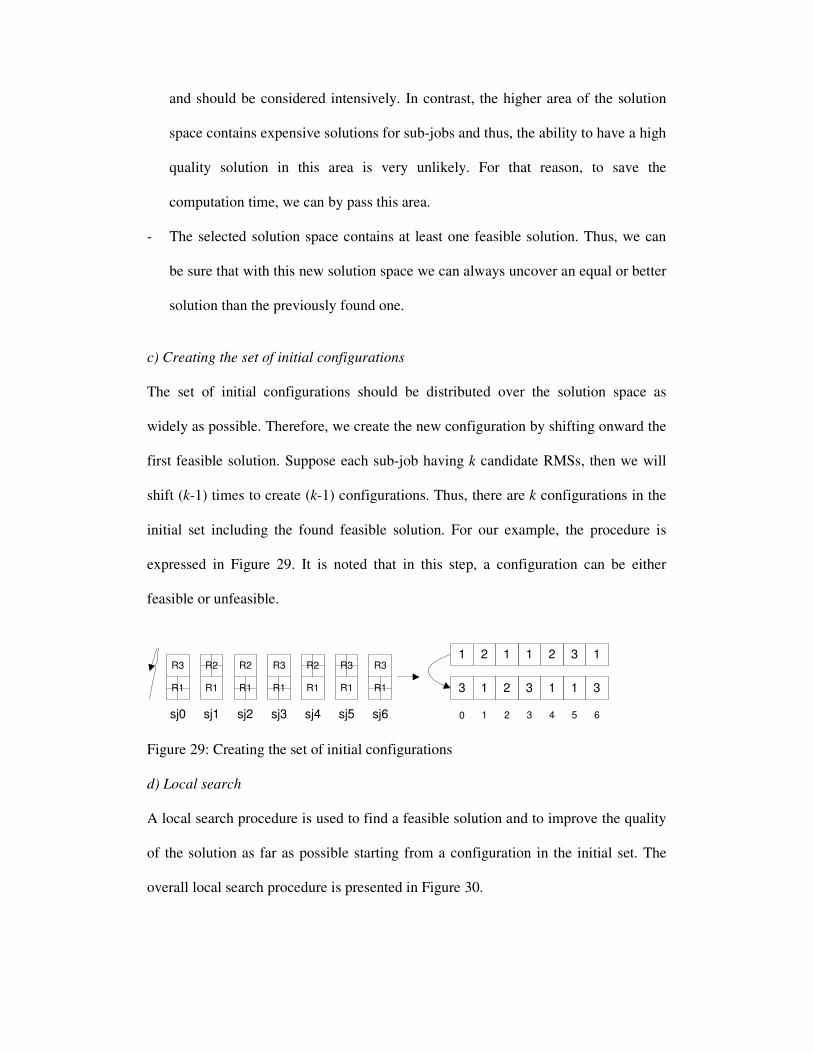
c) Creating the set of initial configurations The set of initial configurations should be distributed over the solution space as

widely as possible. Therefore, we create the new configuration by shifting onward the

first feasible solution. Suppose each sub-job having k candidate RMSs, then we will

shift (k-1) times to create (k-1) configurations. Thus, there are k configurations in the

initial set including the found feasible solution. For our example, the procedure is

expressed in Figure 29. It is noted that in this step, a configuration can be either

feasible or unfeasible.

R1

R3

R1

R2

R1

R2

R1

R3

sj1 sj2 sj3 sj4

R1

R2

R1

R3

R1

R3

sj0 sj5 sj6

1 32112 1

0 2 4 51 63

3 11321 3

Figure 29: Creating the set of initial configurations d) Local search A local search procedure is used to find a feasible solution and to improve the quality

of the solution as far as possible starting from a configuration in the initial set. The

overall local search procedure is presented in Figure 30.

Compute cost c of the configuration awhile (1) { For each neighbor in the neighborhood set of a{ if a is feasible compute cost c’ of the neighbor if c’<c put to the list of candidate else compute finished time p’ of the neighbor if p’< deadline compute cost c’ of the neighbor

put to the list of candidate } if the list empty -> stop local search Sort the list If a is not feasible Replace a by the first solution in the list else for each candidate a’ in the list compute finished time p’ if p’< deadline replace a by a’ and break out the loop}

Figure 30: The local search procedure If the initial configuration is not feasible, we search in the neighborhood of the

candidate configuration for feasible solutions satisfying Criterion 4 and 5. Then we

replace the initial one by the best quality solution found. In this case we have to

compute the timetable and check the deadline of all configuration in the

neighborhood.

If the initial configuration is feasible, we then consider only configurations having

less cost than the present solution. Therefore, instead of computing the cost and the

timetable of all configurations in the neighborhood set at the same time, we only

compute the cost of each configuration individually. All the configurations are stored

in a sorted list. We then compute the timetable of the less expensive configurations

along the list to find the first feasible configuration. This technique helps reduce the

algorithm's runtime significantly as the computation timetable procedure takes a

significant time to be completed. The computation timetable procedure is the one in

Figure 9.

The time to perform the local search procedure varies depending on the number of

invoking module computing timetable. If this number is small the computing time

will be short and vice versa.

5. PERFORMANCE EXPERIMENT The performance experiment is done by simulation to check for the quality of the

mapping algorithms. The hardware and software used in the experiments is rather

standard and simple (Pentium 4 2,8Ghz, 2GB RAM, Linux Redhat 9.0, MySQL). The

whole simulation program is implemented in C/C++. We generated several scenarios

with different workflow configurations and different RMS configurations to be

compatible with the ability of the comparing algorithms. The goal of the experiment is

to measure the feasibility, the quality of the solution, and the time needed for the

computation.

5.1 w-Tabu algorithm performance We employed all the ideas in the recently appearing literature related to mapping

workflow to Grid resource with the same destination to minimize the finished time

and adapted them to our problem. Those algorithms include w-DCP, Grasp, minmin,

maxmin, and suffer (Quan, 2006). To compare the quality of all the described

algorithms above, we generated 18 different workflows which:

- Have different topologies.

- Have a different number of sub-jobs. The number of sub-jobs is in the range 7-32.

- Have different sub-job specifications.

- Have different amounts of data transfer. The amount of data transfer is in the

range from several hundred MB to several GB.

In the algorithms, the number of the sub-job is the most important factor to the

execution time of the algorithm. We also stop at 32 sub-jobs for a workflow because

as far as we know, with our model of parallel task sub-job, most existing Grid-based

workflows include only 10-20 sub-jobs. Thus, we believe that our workload

configuration can simulate accurately the requirement of real problems. Those

workflows will be mapped to 20 RMSs with different resource configurations and

different resource reservation contexts. The workflows are mapped by 6 algorithms

w-Tabu, w-DCP, Grasp, minmin, maxmin, and suffer. The finished time and the

runtime of solutions generated by each algorithm correlative with each workflow are

recorded.

The experimental data shows that all algorithms need few seconds to find out the

solutions. The overall quality comparison among algorithms is depicted in Figure 31.

The graph presents the average relative values of the solution’s finished time created

by different algorithms. From Figure 31, it can be seen that our algorithm outperforms

all other algorithms.

0

0,2

0,4

0,6

0,8

1

1,2

1,4

1,6

w-Tabu Minmin Maxmin Suffer w-DCP GRASP

Ave

rage

fini

shed

tim

e ra

te

Figure 31: Overall quality comparison of w-Tabu and other algorithms

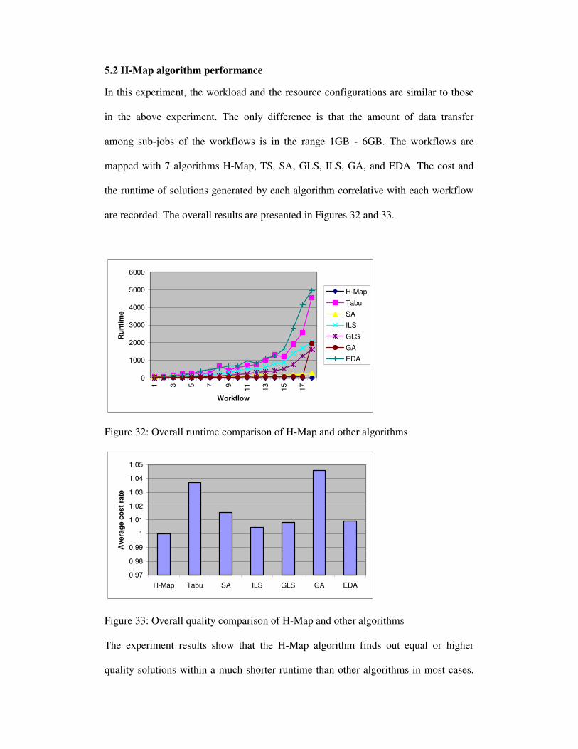
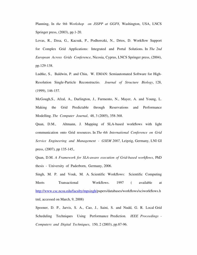
5.2 H-Map algorithm performance

In this experiment, the workload and the resource configurations are similar to those

in the above experiment. The only difference is that the amount of data transfer

among sub-jobs of the workflows is in the range 1GB - 6GB. The workflows are

mapped with 7 algorithms H-Map, TS, SA, GLS, ILS, GA, and EDA. The cost and

the runtime of solutions generated by each algorithm correlative with each workflow

are recorded. The overall results are presented in Figures 32 and 33.

0

1000

2000

3000

4000

5000

6000

1 3 5 7 9 11 13 15 17

Workflow

Run

time

H-Map

Tabu

SA

ILS

GLS

GA

EDA

Figure 32: Overall runtime comparison of H-Map and other algorithms

0,97

0,98

0,99

1

1,01

1,02

1,03

1,04

1,05

H-Map Tabu SA ILS GLS GA EDA

Ave

rage

cos

t rat

e

Figure 33: Overall quality comparison of H-Map and other algorithms The experiment results show that the H-Map algorithm finds out equal or higher

quality solutions within a much shorter runtime than other algorithms in most cases.

With small-scale problems, some metaheuristics using local search such as ILS, GLS,

and EDA find out equal results with the H-Map and better than the SA or GA. But

with large-scale problems, they have an exponential runtime with unsatisfactory

results.

5.3 L-Map algorithm performance In this experiment, the resource configurations are similar to those in the above

experiment. The workload includes 20 workflows. They are different in topologies,

sub-jobs configuration. The number of sub-jobs is from 21 to 32. The amount of data

transfer among sub-jobs of the workflows is in the range 1MB – 10MB. The

workflows are mapped to resources with 4 algorithms L-Map, H-Map, DBC, and GA.

The cost and the runtime of solutions generated by each algorithm correlative with

each workflow are recorded. The overall results are presented in Figure 34 and Figure

35

05

101520253035404550

L-Map H-Map DBC GA

Ave

rage

run

time

Figure 34: Overall runtime comparison of L-Map and other algorithms

From the results, we can see that the L-Map algorithm created higher quality solutions

than all comparing algorithms. Compares to H-Map and GS algorithms, the quality of

L-Map algorithm is slightly better but the runtime is significantly smaller. The cost

difference between solutions found by the L-Map algorithm and the DBC algorithm is

small in absolute value. However, when we examine the difference within a business

context and a business model, it will have significant meaning. From the business

point of view, the broker does the mapping and the income is more important than the

total cost of running the workflow. Assuming that the workflow execution service

counts for 5% of the total running cost, the broker using the L-map algorithm will

have the income 6% higher than the broker using the DBC algorithm. Moreover,

experimenting the negotiation period of the SLA workflow with Web service

technology, each negotiation round took a minute or more, mainly for user checking

the differences in SLA content. Thus, in our opinion, the runtime of the L-Map

algorithm is well acceptable in practical with just few seconds.

18831884188518861887188818891890189118921893

L-Map H-Map DBC GA

Ave

rage

cos

t

Figure 34: Overall quality comparison of L-Map and other algorithms 6. CONCLUSION This chapter has presented concepts and algorithms of mapping Grid-based workflow

to Grid resources within the Service Level Agreement context. The Grid-based

workflow under Directed Acyclic Graph format includes many dependent sub-jobs

which can be either a sequential or parallel application. The Service Level Agreement

context implies a business Grid with many providers which are High Performance

Computing Centers. Each High Performance Computing Center supports resource

reservation and bandwidth reservation. The business Grid leads to the mapping with

the cost optimization problem. To solve the problem, with each workflow

characteristic and Grid resource state, a different specific algorithm is used. If there

are a lot of Grid resources free, L-Map or H-Map algorithm is called on to find the

cost-optimal solution. If there are few Grid resources free, w-Tabu is called on to find

a feasible solution. The set of those algorithms could be employed as the heart of the

system supporting Service Level Agreement for the Grid-based workflow.

REFERENCES Berriman, G. B., Good, J. C., Laity, A. C. (2003) Montage: a Grid Enabled Image

Mosaic Service for the National Virtual Observatory. ADASS, 13, (2003),145-1

167.

Brandic, I., Benkner, S., Engelbrecht, G. and Schmidt, R. QoS Support for Time-

Critical Grid Workflow Applications. In The first International Conference on e-

Science and Grid Computing 2005, Melbourne, Australia, IEEE Computer Society

Press, (2005), pp.108-115.

Deelman, E., Blythe, J., Gil, Y., Kesselman, C., Mehta, G., Patil, S., Su, M., Vahi,

K. and Livny, M. Pegasus : Mapping Scientific Workflows onto the Grid. In The 2nd

European Across Grids Conference, Nicosia, Cyprus, LNCS Springer press,

(2004), pp.11-20.

Fischer, L. Workflow Handbook 2004, Future Strategies Inc., Lighthouse Point, FL,

USA.

Georgakopoulos, D., Hornick, M., and Sheth, A. An Overview of workflow

management: From Process Modeling to Workflow Automation Infrastructure,

Distributed and Parallel Databases, 3, 2 (1995), 119-153.

Hovestadt, M. Scheduling in HPC Resource Management Systems:Queuing vs.

Planning, In the 9th Workshop on JSSPP at GGF8, Washington, USA, LNCS

Springer press, (2003), pp.1-20.

Lovas, R., Dzsa, G., Kacsuk, P., Podhorszki, N., Drtos, D. Workflow Support

for Complex Grid Applications: Integrated and Portal Solutions. In The 2nd

European Across Grids Conference, Nicosia, Cyprus, LNCS Springer press, (2004),

pp.129-138.

Ludtke, S., Baldwin, P. and Chiu, W. EMAN: Semiautomated Software for High-

Resolution Single-Particle Reconstructio. Journal of Structure Biology, 128,

(1999), 146-157.

McGough,S., Afzal, A., Darlington, J., Furmento, N., Mayer, A. and Young, L.

Making the Grid Predictable through Reservations and Performance

Modelling. The Computer Journal, 48, 3 (2005), 358-368.

Quan, D.M., Altmann, J. Mapping of SLA-based workflows with light

communication onto Grid resources. In The 4th International Conference on Grid

Service Engineering and Management - GSEM 2007, Leipzig, Germany, LNI GI

press, (2007), pp 135-145,.

Quan, D.M. A Framework for SLA-aware execution of Grid-based workflows, PhD

thesis - University of Paderborn, Germany, 2006.

Singh, M. P. and Vouk, M. A. Scientific Workflows: Scientific Computing

Meets Transactional Workflows. 1997 ( available at

http://www.csc.ncsu.edu/faculty/mpsingh/papers/databases/workflows/sciworkflows.h

tml, accessed on March, 9, 2008)

Spooner, D. P., Jarvis, S. A., Cao, J., Saini, S. and Nudd, G. R. Local Grid

Scheduling Techniques Using Performance Prediction. IEEE Proceedings -

Computers and Digital Techniques, 150, 2 (2003), pp.87-96.

Wolski, R. Experiences with Predicting Resource Performance On-line in

Computational Grid Settings. ACM SIGMETRICS Performance Evaluation Review,

30, 4 (2003), 41-49.

Zeng, L., Benatallah, B., Ngu, A., Dumas, M., Kalagnanam, J., Chang, H.

QoS-Aware Middleware for Web Services Composition. IEEE Transactions on

Software Engineering, 30, 5 (2004), 311-327.