Hexagonal Grid Image Processing Algorithms in Neural Vision …paginas.fe.up.pt/~tavares/downloads/publications/relatorios/bio... · Hexagonal Grid Image Processing Algorithms in

Hexagonal Grid Image ProcessingAlgorithms in Neural Vision and Prediction

NUNO ALBUQUERQUE SOUSAFaculdade de Engenharia da Universidade do Porto

June 6, 2014

Abstract

In the field of neural prediction of the visual cortex, it is known that97%[1]of receptive field neurons are described by the response to a 3DGabor Filter (2D over time). By replacing the stimulus representation- a 2D image with square pixels, with an hexagonal system, someadvantages are theoretically possible: better computational speeds,lower memory footprint, and more accurate depiction of the biologicalphenomena taking place. In this work the framework for handling thealgorithms and operations typical in the neural prediction work floware established, and tested for practicality.

Keywords: Neural Prediction, Hexagonal Image Processing, VisualCortex, Receptive Field, Honeycomb Scheme, Hex Gabor Filtering.

Introduction

This work is the final report of the UC Investigation Techniques, part of thecurricular program of the Doctoral Program in Biomedical Engineering. Thepurpose of this UC is to allow the graduate students to familiarize and gaincompetence with a given technique or techniques. The focus of the workpresented, a technique which is perceived to be of great potential in thefuture PhD thesis, is on the application of an hexagonal tessellation insteadof a quadratic in the representation of the visual stimulus. The advantagesof said change are explored in the Motivations subsection. The broad themeof neural prediction of the visual cortex, is a well established field in itself,and has been the author’s theme of thesis for his MSc. The algorithmsfor classification and prediction are in the author opinion reaching theirbreaking point in terms of improvement. The focus of the new techniques

1

proposed is the first part of the neural prediction work-flow. The process ofneural prediction has usually three stages:

1. Image Analysis and "Feature Extraction"1

2. Classification or Regression

3. Non Linear Filtering

It’s in the first stage where the substitution from a square grid to ahexagonal one is to occur. Then again the algorithms used in the imageanalysis are very well established. However the properties of the hexagonalgrid may be of some use to gain some ground on this field.

Motivations

The advantages of an hexagonal grid to describe the stimulus data (a moviefor instance) over the typical square lattice are:

• The hexagonal pixel is very superior in efficiency, for describing datawith a given resolution.

• The neighborhood of an hexagonal pixel grows at a decreased range:the neighborhood of square pixels grows at 8 per growth, whilehexagons grow at 6 per growth(see figure 1).

• Smaller Quantetization Error [2] - Again, this is useful when workingwith downsampled images for computational reasons as is todayalways2 the case.

• Greater Angular Resolution [2] - In neural prediction 12 directions areusually used, which can be achieved with a 3 layer hex filter, savingcomputational resources.

• Connectivity Definition [3] - There are neighborhood variants, of somefilters which vary between 4 and 8 pixel connectivity in rectangulargrids, this eliminates the problem of choice.

• Equidistance of neighborhood [3] - Better representation of data.

• Higher Symmetry [4] - No foreseeable advantage.

• Most filters are somewhat circular, or at least directional, and giventhat the neighborhood also grows with some circularity, hexagonalfiltering is computationally more efficient.

• Fewer Sampling Points [5] - Computational Efficiency

1The features are usually the magnitude of the response of a region of the image to a filter2Today’s algorithms are so heavy, and the Gabor Wavelet Processing so time consuming,

there is hardly any chance of using original size stimulus files

2

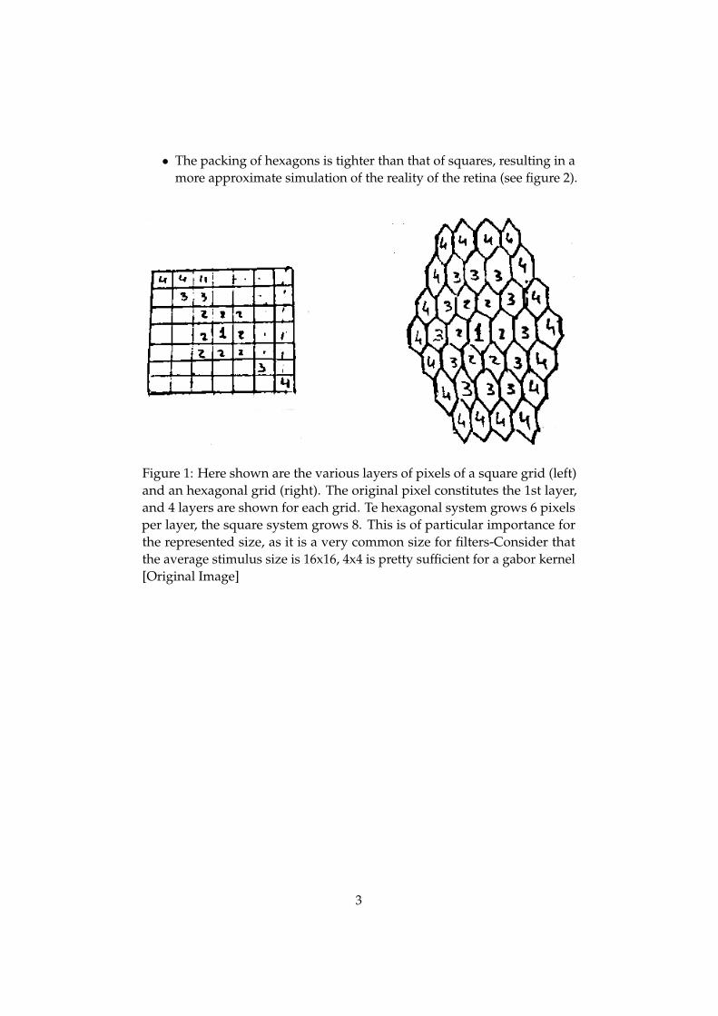
• The packing of hexagons is tighter than that of squares, resulting in amore approximate simulation of the reality of the retina (see figure 2).

Figure 1: Here shown are the various layers of pixels of a square grid (left)and an hexagonal grid (right). The original pixel constitutes the 1st layer,and 4 layers are shown for each grid. Te hexagonal system grows 6 pixelsper layer, the square system grows 8. This is of particular importance forthe represented size, as it is a very common size for filters-Consider thatthe average stimulus size is 16x16, 4x4 is pretty sufficient for a gabor kernel[Original Image]

3

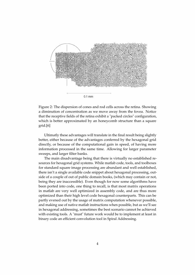
Figure 2: The dispersion of cones and rod cells across the retina. Showinga diminution of concentration as we move away from the fovea. Noticethat the receptive fields of the retina exhibit a "packed circles" configuration,which is better approximated by an honeycomb structure than a squaregrid.[6]

Ultimatly these advantages will translate in the final result being slightlybetter, either because of the advantages conferred by the hexagonal griddirectly, or because of the computational gain in speed, of having moreinformation processed in the same time. Allowing for larger parametersweeps, and larger filter banks.

The main disadvantage being that there is virtually no established re-sources for hexagonal grid systems. While matlab code, tools, and toolboxesfor standard square image processing are abundant and well established,there isn’t a single available code snippet about hexagonal processing, out-side of a couple of out of public domain books, (which may contain or not,being they are inaccessible). Even though for now some algorithms havebeen ported into code, one thing to recall, is that most matrix operationsin matlab are very well optimized in assembly code, and are thus moreoptimized than their high level code hexagonal counterparts. This can bepartly evened out by the usage of matrix computation whenever possible,and making use of native matlab instructions when possible, but as we’ll seein hexagonal addressing, sometimes the best scenario cannot be achievedwith existing tools. A "must" future work would be to implement at least inbinary code an efficient convolution tool in Spiral Addressing.

4

State of the Art

The idea of applying hexagonal grid to the mechanisms of vision processingis not entirely novel: several areas of computer vision are already well fa-miliar with the idea, so there is mathematical background into hexagonallattices sufficient for our needs. The application of said grids into cognitiveneuroscience is novel, however there is a 2012 PhD Thesis which handles asimilar area on the topic[7]3. Applications of hexagonal grid in biomedicalengineering include, in a different aspect of image processing the recon-struction of tomography images into a 3D model[8]. The advantages ofthe hexagon are paragon when solving the complicated equations of imagereconstruction.

Perhaps of singular importance would be the application of gabor waveletsin hexagonal grids. The work on this particular subject is existent, and giventhat the response to gabor filter banks is the current state of the art approachfor neural prediction, the elaboration of 3D gabor wavelets hexagonally willbe the ultimate goal in this work.

Hexagonal Grid Framework

One of the conclusions that this work must reach is wether or not HexagonalGrid is best suited for the given applications.

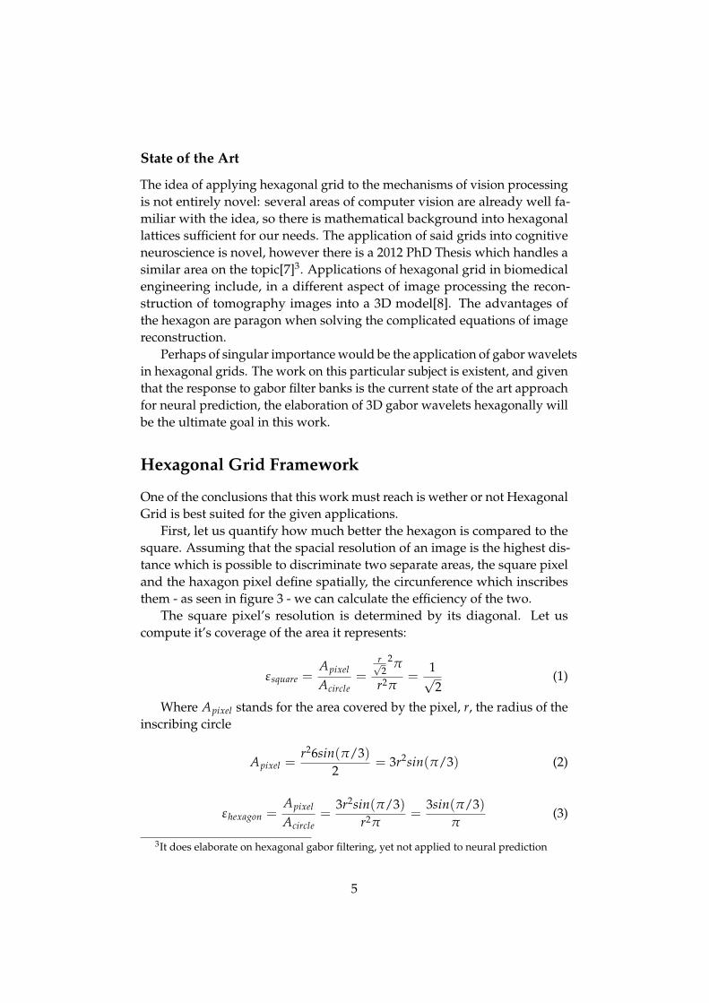
First, let us quantify how much better the hexagon is compared to thesquare. Assuming that the spacial resolution of an image is the highest dis-tance which is possible to discriminate two separate areas, the square pixeland the haxagon pixel define spatially, the circunference which inscribesthem - as seen in figure 3 - we can calculate the efficiency of the two.

The square pixel’s resolution is determined by its diagonal. Let uscompute it’s coverage of the area it represents:

εsquare =Apixel

Acircle=

r√2

2π

r2π=

1√2

(1)

Where Apixel stands for the area covered by the pixel, r, the radius of theinscribing circle

Apixel =r26sin(π/3)

2= 3r2sin(π/3) (2)

εhexagon =Apixel

Acircle=

3r2sin(π/3)r2π

=3sin(π/3)

π(3)

3It does elaborate on hexagonal gabor filtering, yet not applied to neural prediction

5

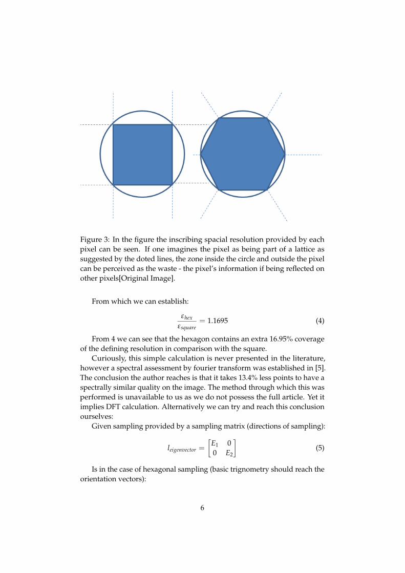
Figure 3: In the figure the inscribing spacial resolution provided by eachpixel can be seen. If one imagines the pixel as being part of a lattice assuggested by the doted lines, the zone inside the circle and outside the pixelcan be perceived as the waste - the pixel’s information if being reflected onother pixels[Original Image].

From which we can establish:

εhex

εsquare= 1.1695 (4)

From 4 we can see that the hexagon contains an extra 16.95% coverageof the defining resolution in comparison with the square.

Curiously, this simple calculation is never presented in the literature,however a spectral assessment by fourier transform was established in [5].The conclusion the author reaches is that it takes 13.4% less points to have aspectrally similar quality on the image. The method through which this wasperformed is unavailable to us as we do not possess the full article. Yet itimplies DFT calculation. Alternatively we can try and reach this conclusionourselves:

Given sampling provided by a sampling matrix (directions of sampling):

leigenvector =

[E1 00 E2

](5)

Is in the case of hexagonal sampling (basic trignometry should reach theorientation vectors):

6

leigenvector =

[E1 E1/20√

3E1/2

](6)

In equation 6 the second column are the x and y projections of thesecond vector. (Imagine it pointing from the first hexagon onto the top rightneighbor for visualization)

From this we can establish the sampling in the spectral domain:

LT l = I (7)

Where I is the identity matrix.Simple algebra returns:

Lhex =

[2πE1

0− 2π√

3E1

4π√3E1

](8)

Knowing that the maximum frequency those pixels can define is thecircle that inscribes them and touches them at the diagonal, we can equatethis circle in terms of spectral frequency.

4π√3E1

= 2W (9)

Bringing the equality back to the spatial domain yelds:

lquadrado =

[πW 00 π

W

](10)

And for the hexagon:

lhexagono =

[2π√3W

π√3W

0 πW

](11)

In this spatial form, we know that the necessary sizes for this spatialrepresentation of the frequency W, therefor, we need only find the ratiobetween the two magnitudes of the vectors, which may be found by thedeterminant of their matrices. By computing the ratio between the two, wecan present:

|detlquadrado||detlhexagono|

=

√3

2= 0.87 (12)

There are needed only 87% of the samples in an hexagon grid to dis-criminate with the same accuracy what the full 100% grid of squares wouldsignify.

The computation based on the area, and the spectral area should berelated, though the author is not entirely sure how.

7

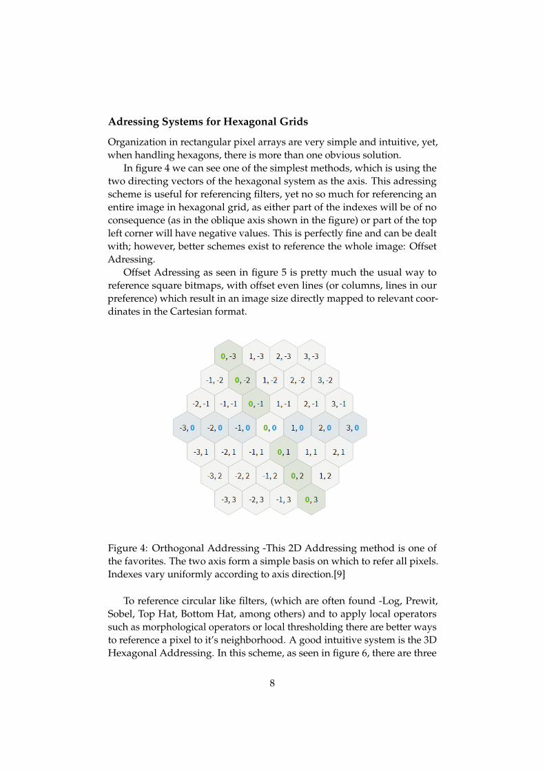
Adressing Systems for Hexagonal Grids

Organization in rectangular pixel arrays are very simple and intuitive, yet,when handling hexagons, there is more than one obvious solution.

In figure 4 we can see one of the simplest methods, which is using thetwo directing vectors of the hexagonal system as the axis. This adressingscheme is useful for referencing filters, yet no so much for referencing anentire image in hexagonal grid, as either part of the indexes will be of noconsequence (as in the oblique axis shown in the figure) or part of the topleft corner will have negative values. This is perfectly fine and can be dealtwith; however, better schemes exist to reference the whole image: OffsetAdressing.

Offset Adressing as seen in figure 5 is pretty much the usual way toreference square bitmaps, with offset even lines (or columns, lines in ourpreference) which result in an image size directly mapped to relevant coor-dinates in the Cartesian format.

Figure 4: Orthogonal Addressing -This 2D Addressing method is one ofthe favorites. The two axis form a simple basis on which to refer all pixels.Indexes vary uniformly according to axis direction.[9]

To reference circular like filters, (which are often found -Log, Prewit,Sobel, Top Hat, Bottom Hat, among others) and to apply local operatorssuch as morphological operators or local thresholding there are better waysto reference a pixel to it’s neighborhood. A good intuitive system is the 3DHexagonal Addressing. In this scheme, as seen in figure 6, there are three

8

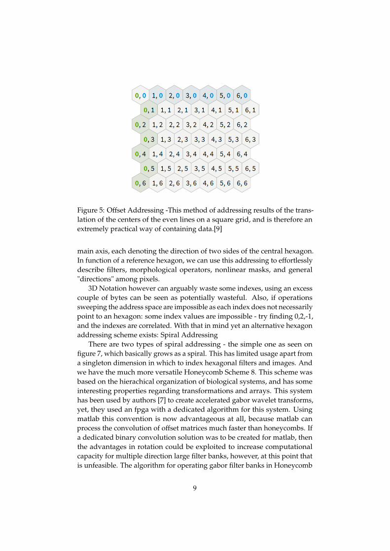
Figure 5: Offset Addressing -This method of addressing results of the trans-lation of the centers of the even lines on a square grid, and is therefore anextremely practical way of containing data.[9]

main axis, each denoting the direction of two sides of the central hexagon.In function of a reference hexagon, we can use this addressing to effortlesslydescribe filters, morphological operators, nonlinear masks, and general"directions" among pixels.

3D Notation however can arguably waste some indexes, using an excesscouple of bytes can be seen as potentially wasteful. Also, if operationssweeping the address space are impossible as each index does not necessarilypoint to an hexagon: some index values are impossible - try finding 0,2,-1,and the indexes are correlated. With that in mind yet an alternative hexagonaddressing scheme exists: Spiral Addressing

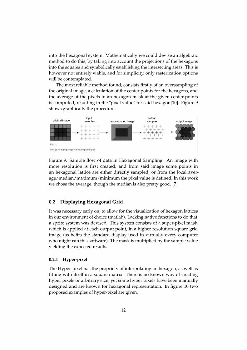
There are two types of spiral addressing - the simple one as seen onfigure 7, which basically grows as a spiral. This has limited usage apart froma singleton dimension in which to index hexagonal filters and images. Andwe have the much more versatile Honeycomb Scheme 8. This scheme wasbased on the hierachical organization of biological systems, and has someinteresting properties regarding transformations and arrays. This systemhas been used by authors [7] to create accelerated gabor wavelet transforms,yet, they used an fpga with a dedicated algorithm for this system. Usingmatlab this convention is now advantageous at all, because matlab canprocess the convolution of offset matrices much faster than honeycombs. Ifa dedicated binary convolution solution was to be created for matlab, thenthe advantages in rotation could be exploited to increase computationalcapacity for multiple direction large filter banks, however, at this point thatis unfeasible. The algorithm for operating gabor filter banks in Honeycomb

9

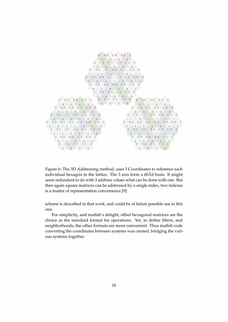
Figure 6: The 3D Addressing method, uses 3 Coordinates to reference eachindividual hexagon in the lattice. The 3 axis form a 60ž basis. It mightseem redundant to do with 3 address values what can be done with one. Butthen again square matrices can be addressed by a single index, two indexesis a matter of representation convenience.[9]

scheme is described in that work, and could be of future possible use in thisone.

For simplicity, and matlab’s delight, offset hexagonal matrices are thechoice as the standard format for operations. Yet, to define filters, andneighborhoods, the other formats are more convenient. Thus matlab codeconverting the coordinates between systems was created, bridging the vari-ous systems together.

10

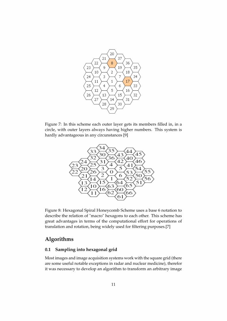
Figure 7: In this scheme each outer layer gets its members filled in, in acircle, with outer layers always having higher numbers. This system ishardly advantageous in any circunstances [9]

Figure 8: Hexagonal Spiral Honeycomb Scheme uses a base 6 notation todescribe the relation of "macro" hexagons to each other. This scheme hasgreat advantages in terms of the computational effort for operations oftranslation and rotation, being widely used for filtering purposes.[7]

Algorithms

0.1 Sampling into hexagonal grid

Most images and image acquisition systems work with the square grid (thereare some useful notable exceptions in radar and nuclear medicine), thereforit was necessary to develop an algorithm to transform an arbitrary image

11

into the hexagonal system. Mathematically we could devise an algebraicmethod to do this, by taking into account the projections of the hexagonsinto the squares and symbolically establishing the intersecting areas. This ishowever not entirely viable, and for simplicity, only rasterization optionswill be contemplated.

The most reliable method found, consists firstly of an oversampling ofthe original image, a calculation of the center points for the hexagons, andthe average of the pixels in an hexagon mask at the given center pointsis computed, resulting in the "pixel value" for said hexagon[10]. Figure 9shows graphically the procedure.

Figure 9: Sample flow of data in Hexagonal Sampling. An image withmore resolution is first created, and from said image some points inan hexagonal lattice are either directly sampled, or from the local aver-age/median/maximum/minimum the pixel value is defined. In this workwe chose the average, though the median is also pretty good. [7]

0.2 Displaying Hexagonal Grid

It was necessary early on, to allow for the visualization of hexagon latticesin our environment of choice (matlab). Lacking native functions to do that,a sprite system was devised. This system consists of a super-pixel mask,which is applied at each output point, in a higher resolution square gridimage (as befits the standard display used in virtually every computerwho might run this software). The mask is multiplied by the sample valueyielding the expected results.

0.2.1 Hyper-pixel

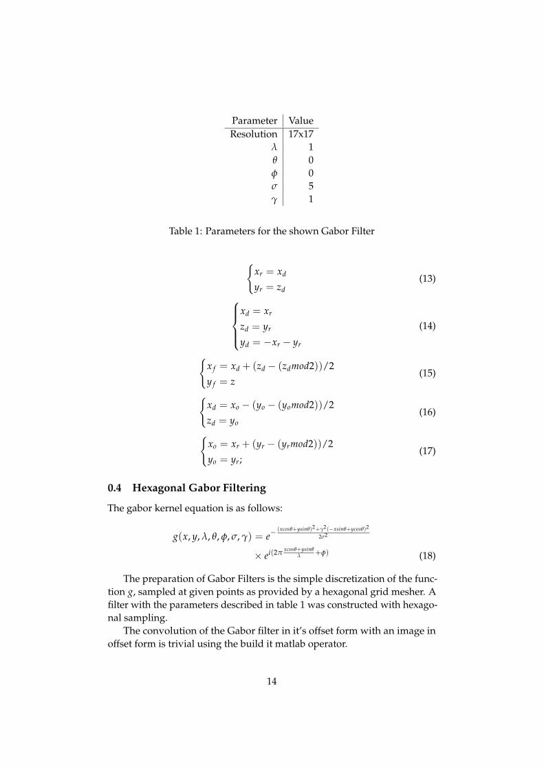
The Hyper-pixel has the propriety of interpolating an hexagon, as well asfitting with itself in a square matrix. There is no known way of creatinghyper pixels or arbitrary size, yet some hyper pixels have been manuallydesigned and are known for hexagonal representation. In figure 10 twoproposed examples of hyper-pixel are given.

12

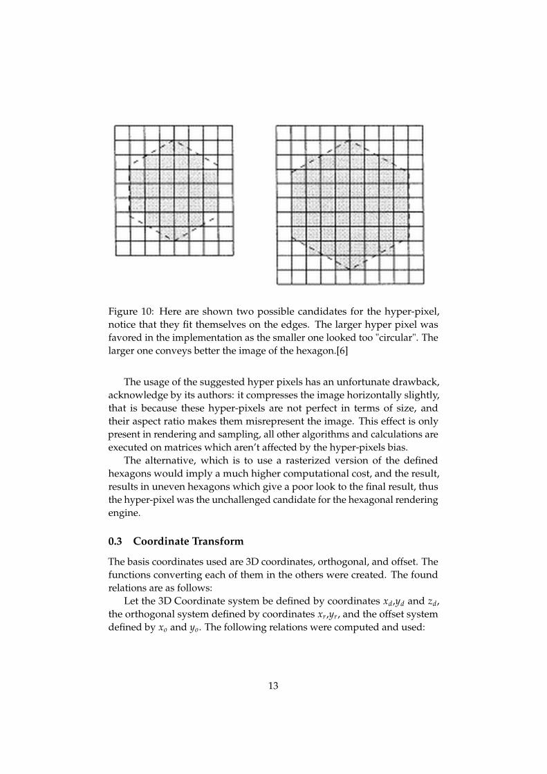
Figure 10: Here are shown two possible candidates for the hyper-pixel,notice that they fit themselves on the edges. The larger hyper pixel wasfavored in the implementation as the smaller one looked too "circular". Thelarger one conveys better the image of the hexagon.[6]

The usage of the suggested hyper pixels has an unfortunate drawback,acknowledge by its authors: it compresses the image horizontally slightly,that is because these hyper-pixels are not perfect in terms of size, andtheir aspect ratio makes them misrepresent the image. This effect is onlypresent in rendering and sampling, all other algorithms and calculations areexecuted on matrices which aren’t affected by the hyper-pixels bias.

The alternative, which is to use a rasterized version of the definedhexagons would imply a much higher computational cost, and the result,results in uneven hexagons which give a poor look to the final result, thusthe hyper-pixel was the unchallenged candidate for the hexagonal renderingengine.

0.3 Coordinate Transform

The basis coordinates used are 3D coordinates, orthogonal, and offset. Thefunctions converting each of them in the others were created. The foundrelations are as follows:

Let the 3D Coordinate system be defined by coordinates xd,yd and zd,the orthogonal system defined by coordinates xr,yr, and the offset systemdefined by xo and yo. The following relations were computed and used:

13

Parameter ValueResolution 17x17

λ 1θ 0φ 0σ 5γ 1

Table 1: Parameters for the shown Gabor Filter

{xr = xd

yr = zd(13)

xd = xr

zd = yr

yd = −xr − yr

(14)

{x f = xd + (zd − (zdmod2))/2

y f = z(15)

{xd = xo − (yo − (yomod2))/2

zd = yo(16)

{xo = xr + (yr − (yrmod2))/2

yo = yr;(17)

0.4 Hexagonal Gabor Filtering

The gabor kernel equation is as follows:

g(x, y, λ, θ, φ, σ, γ) = e−(xcosθ+ysinθ)2+γ2(−xsinθ+ycosθ)2

2σ2

× ei(2πxcosθ+ysinθ

λ +φ) (18)

The preparation of Gabor Filters is the simple discretization of the func-tion g, sampled at given points as provided by a hexagonal grid mesher. Afilter with the parameters described in table 1 was constructed with hexago-nal sampling.

The convolution of the Gabor filter in it’s offset form with an image inoffset form is trivial using the build it matlab operator.

14

Results

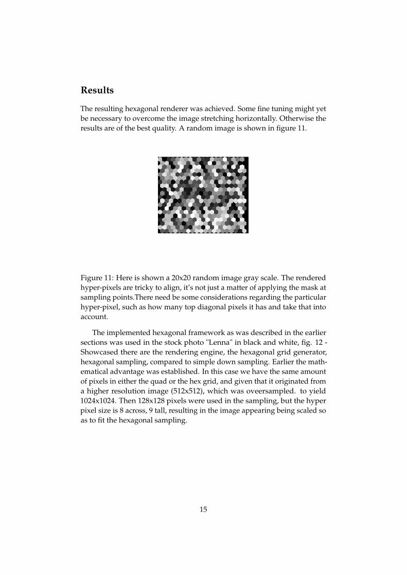
The resulting hexagonal renderer was achieved. Some fine tuning might yetbe necessary to overcome the image stretching horizontally. Otherwise theresults are of the best quality. A random image is shown in figure 11.

Figure 11: Here is shown a 20x20 random image gray scale. The renderedhyper-pixels are tricky to align, it’s not just a matter of applying the mask atsampling points.There need be some considerations regarding the particularhyper-pixel, such as how many top diagonal pixels it has and take that intoaccount.

The implemented hexagonal framework as was described in the earliersections was used in the stock photo "Lenna" in black and white, fig. 12 -Showcased there are the rendering engine, the hexagonal grid generator,hexagonal sampling, compared to simple down sampling. Earlier the math-ematical advantage was established. In this case we have the same amountof pixels in either the quad or the hex grid, and given that it originated froma higher resolution image (512x512), which was oveersampled. to yield1024x1024. Then 128x128 pixels were used in the sampling, but the hyperpixel size is 8 across, 9 tall, resulting in the image appearing being scaled soas to fit the hexagonal sampling.

15

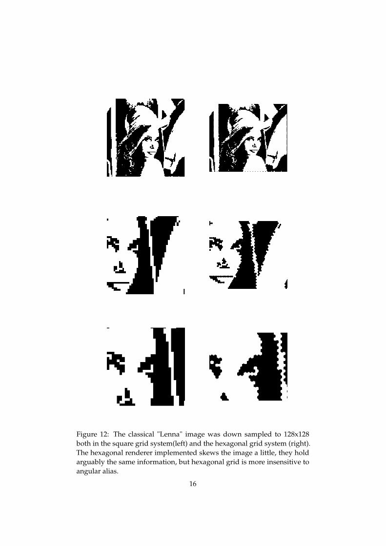
Figure 12: The classical "Lenna" image was down sampled to 128x128both in the square grid system(left) and the hexagonal grid system (right).The hexagonal renderer implemented skews the image a little, they holdarguably the same information, but hexagonal grid is more insensitive toangular alias.

16

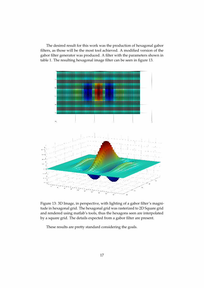
The desired result for this work was the production of hexagonal gaborfilters, as those will be the most tool achieved. A modified version of thegabor filter generator was produced. A filter with the parameters shown intable 1. The resulting hexagonal image filter can be seen in figure 13.

Figure 13: 3D Image, in perspective, with lighting of a gabor filter’s magni-tude in hexagonal grid. The hexagonal grid was rasterized to 2D Square gridand rendered using matlab’s tools, thus the hexagons seen are interpolatedby a square grid. The details expected from a gabor filter are present.

These results are pretty standard considering the goals.

17

Conclusions

The visual inspection of a square grid versus an hexagonal grid show thatthe latter can convey more information with the same amount of pixels.

As a byproduct of this work some tools have been developed (and forreference there were none available) which enable among other things tooperate with hexagonal imaging. A promised future work will be to grindand make more universal said tools, so as to allow the production of aMatlab toolbox. Details on the work to be done can be found in the futurework section.

These improvements in processing will hopefully translate in at leastbetter computational performance once incorporated in the main algorithmsof neural prediction. The shown quality for lesser pixels cannot be stressedenough, as computational times for 128x128 images are prohibitive, andthe computational cost scales with the 3rd power of the size of the imagestimulus, so using more filters in less pixels will be advantageous for overallquality.

One simple general conclusion is that hexagonal processing brings manyadvantages, but at a cost of minutiae details which are normally insufferable.If one is considering hex usage for vision applications outside of the aca-demic domain; the bothersome roadblocks will become prohibitive as oneconsiders one’s ideas more interesting that fighting a rather cumbersomesystem which will provide plenty of out of bounds indexes. Yet it can rewardin the end as well.

Future Work

A Natural Development of the referred topics, is to incorporate this stage ofprocessing into the broader picture, that is to say, use the achieved results inthe next phases of neural prediction processing. That and other work willbe subject of the PhD thesis.

A toolbox with the implemented functions is to be prepared for thecommunity. For such purposes the code must be adapted, for instance, as ofnow, it doesn’t support color, as stimulus in the neural prediction dataset areusually gray scale. The code listing can be found in http://paginas.fe.up.

pt/~bio08062. It includes hexagonal rendering engine, various coordinateconverters, an hexagonal grid sampler, an hexagonal mesh tool (similar to"gridmesh") and an hexagonal 3D Gabor tool.

18

References

1. P. Dayan and L.F. Abbott. Theoretical neuroscience, volume 31. MIT pressCambridge, MA, 2001.

2. Behzad Kamgar-Parsi. Quantization error in hexagonal sensory config-urations. Pattern Analysis and Machine Intelligence, IEEE Transactions on,14(6):665–671, 1992.

3. Xiangjian He and Wenjing Jia. Hexagonal structure for intelligent vision.In Information and Communication Technologies, 2005. ICICT 2005. FirstInternational Conference on, pages 52–64. IEEE, 2005.

4. Jean Serra. Introduction to mathematical morphology. Computer vision,graphics, and image processing, 35(3):283–305, 1986.

5. Russell M Mersereau. The processing of hexagonally sampled two-dimensional signals. Proceedings of the IEEE, 67(6):930–949, 1979.

6. Lee Middleton and Jayanthi Sivaswamy. Hexagonal image processing: Apractical approach. Springer, 2006.

7. Barun Kumar and Er Pooja Kaushik. Vision-based hexagonal imageprocessing based hexagonal image processing based hexagonal imageprocessing.

8. Samuel Matej, Avi Vardi, Gabor T Herman, and Eilat Vardi. Binarytomography using gibbs priors. In Discrete Tomography, pages 191–212.Springer, 1999.

9. Red Blob Games. Hexagonal Grids, Mar 2013 (accessed June,4 2014).http://http://www.redblobgames.com/grids/hexagons/.

10. Richard C Staunton. The processing of hexagonally sampled images.Adv. Imaging Electron Phys, 119:191–265, 2001.

19