Concentration dependent refractive index of a binary mixture ...

HAL Id: hal-00683950https://hal.archives-ouvertes.fr/hal-00683950

Submitted on 17 Jan 2022

HAL is a multi-disciplinary open accessarchive for the deposit and dissemination of sci-entific research documents, whether they are pub-lished or not. The documents may come fromteaching and research institutions in France orabroad, or from public or private research centers.

L’archive ouverte pluridisciplinaire HAL, estdestinée au dépôt et à la diffusion de documentsscientifiques de niveau recherche, publiés ou non,émanant des établissements d’enseignement et derecherche français ou étrangers, des laboratoirespublics ou privés.

Concentration dependent refractive index of a binarymixture at high pressure

Fabrizio Croccolo, Marc Alexandre Arnaud, Didier Bégué, Henri Bataller

To cite this version:Fabrizio Croccolo, Marc Alexandre Arnaud, Didier Bégué, Henri Bataller. Concentration dependentrefractive index of a binary mixture at high pressure. Journal of Chemical Physics, American Instituteof Physics, 2011, 135 (3), pp.Article number 034901. �10.1063/1.3610368�. �hal-00683950�

Concentration dependent refractive index of a binary mixtureat high pressure

Fabrizio Croccolo,1,a) Marc-Alexandre Arnaud,2 Didier Bégué,2 and Henri Bataller1,b)

1Laboratoire des Fluides Complexes - UMR 5150, Université de Pau et des Pays de l’Adour, BP 1155,64013 Pau Cedex, France2Institut Pluridisciplinaire de recherche sur l’Environnement et les Matériaux (IPREM) - UMR 5254,CNRS - Equipe de Chimie Physique, Université de Pau et des Pays de l’Adour, 2 avenue du Président Angot,64053 Pau Cedex 9, France

In the present work binary mixtures of varying concentrations of two miscible hydrocarbons, 1,2,3,4-tetrahydronaphtalene (THN) and n-dodecane (C12), are subjected to increasing pressure up to50 MPa in order to investigate the dependence of the so-called concentration contrast factor (CF),i.e., (∂n/∂c)p,T , on pressure level. The refractive index is measured by means of a Mach-Zehnderinterferometer. The setup and experimental procedure are validated with different pure fluids in thesame pressure range. The refractive index of the THN-C12 mixture is found to vary both over pres-sure and concentration, and the concentration CF is found to exponentially decrease as the pressure isincreased. The measured values of the refractive index and the concentration CFs are compared withvalues obtained by two different theoretical predictions, the well-known Lorentz-Lorenz formula andan alternative one proposed by Looyenga. While the measured refractive indices agree very well withpredictions given by Looyenga, the measured concentration CFs show deviations from the latter ofthe order of 6% and more than the double from the Lorentz-Lorenz predictions.

I. INTRODUCTION

A number of fluid properties and phenomena can beaccurately and conveniently investigated by means of re-fined quantitative optical techniques which take advantageof the use of some, typically coherent, light source. Just togive some examples close to our experience: fluid proper-ties like the mass diffusion coefficient of binary mixtures,1

the Soret coefficient,1–5 phenomena like non-equilibriumfluctuations6–13 have been extensively studied throughtechniques such as Mach-Zehnder interferometry,1 staticand dynamic light scattering,10,11, 14–17 beam deflection,2–5

shadowgraph6,8–10, 12, 13 and other scattering in the near field(SINF) techniques.11, 12, 18–21 In most of the aforementionedcases one needs to know a priori the dependence of the re-fractive index of the liquid under analysis on the relevant pa-rameter (concentration, temperature, etc.) in order to deriveaccurate measurements. This dependence is also commonlyreferred to as the contrast factor (CF) defined as (∂n/∂c)p,T

for the concentration CF and (∂n/∂T )p,c for the temperatureCF. Unfortunately, literature data are not always available forthe mixture of interest, and when available, they are not al-ways of good quality as pointed out previously.22, 23 More-over, data are typically limited to atmospheric pressure, andtheoretical predictions are not always reliable in many practi-cal cases.

a)Present address: Physics Department, University of Fribourg, Ch. DuMusée 3, CH-1700 Fribourg, Switzerland.

b)Electronic mail: [email protected].

Recently, the oil industry has shown great interest instudying transport properties.24 Since conditions under whichcrude oil is found underground imply high pressure (HP) anddiffusion in porous media, it is important to analyze the influ-ence of the pressure and the interaction with a porous mediumon the transport properties of liquid mixtures.25 This is doneto achieve better reliability of the algorithms used for simu-lating the crude oil behavior in oil fields. Nevertheless, ther-mal diffusion data under reservoir conditions are very scarceand not very recent.26, 27 In this view, we are interested in per-forming high-pressure interferometric measurements on bi-nary mixtures stressed by a temperature gradient and goingthrough Soret separation across a porous medium. For doingthis we first attempted to precisely measure the concentrationCF of a binary mixture in a wide pressure range. As a conse-quence we had the need to validate our experimental valueswith a theoretical approach able to account for the effect ofpressure.

The choice of the particular model binary mixture tostudy has been mainly driven by the need of having amixture which is already well characterized at atmosphericpressure,28 and which also provides a strong Soret effect.On this basis the liquid mixture has been chosen as 1,2,3,4-tetrahydronaphtalene (THN)–n-dodecane (n-C12) kept at aconstant temperature Tmean = 25 ◦C.

The remainder of this paper is organized as follows: inSec. II, the experimental setup is described along with de-tails of the high pressure thermodiffusion cell and the inter-ferometric setup; in Sec. III, details are provided for the algo-rithm that allows us to obtain the refractive index as a functionof the pressure and for the procedure to obtain the refractive

Published in

which should be cited to refer to this work.

http

://do

c.re

ro.c

h

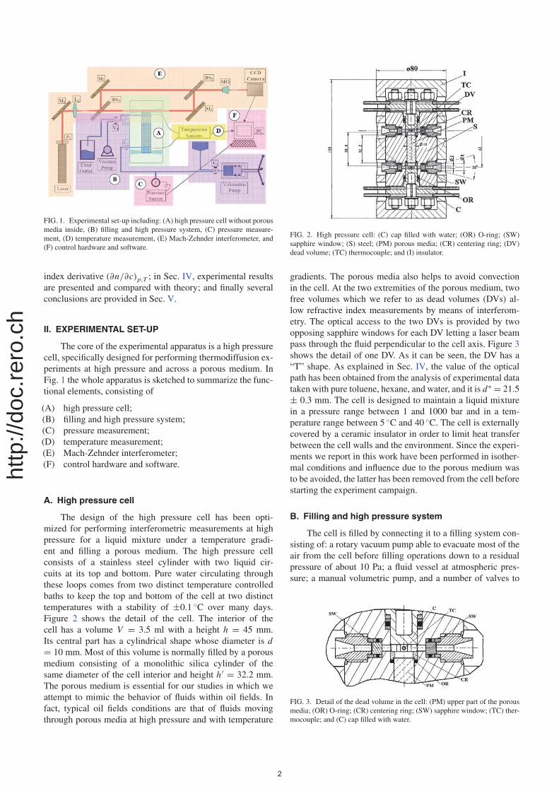
FIG. 1. Experimental set-up including: (A) high pressure cell without porousmedia inside, (B) filling and high pressure system, (C) pressure measure-ment, (D) temperature measurement, (E) Mach-Zehnder interferometer, and(F) control hardware and software.

index derivative (∂n/∂c)p,T ; in Sec. IV, experimental resultsare presented and compared with theory; and finally severalconclusions are provided in Sec. V.

II. EXPERIMENTAL SET-UP

The core of the experimental apparatus is a high pressurecell, specifically designed for performing thermodiffusion ex-periments at high pressure and across a porous medium. InFig. 1 the whole apparatus is sketched to summarize the func-tional elements, consisting of

(A) high pressure cell;(B) filling and high pressure system;(C) pressure measurement;(D) temperature measurement;(E) Mach-Zehnder interferometer;(F) control hardware and software.

A. High pressure cell

The design of the high pressure cell has been opti-mized for performing interferometric measurements at highpressure for a liquid mixture under a temperature gradi-ent and filling a porous medium. The high pressure cellconsists of a stainless steel cylinder with two liquid cir-cuits at its top and bottom. Pure water circulating throughthese loops comes from two distinct temperature controlledbaths to keep the top and bottom of the cell at two distincttemperatures with a stability of ±0.1 ◦C over many days.Figure 2 shows the detail of the cell. The interior of thecell has a volume V = 3.5 ml with a height h = 45 mm.Its central part has a cylindrical shape whose diameter is d= 10 mm. Most of this volume is normally filled by a porousmedium consisting of a monolithic silica cylinder of thesame diameter of the cell interior and height h′ = 32.2 mm.The porous medium is essential for our studies in which weattempt to mimic the behavior of fluids within oil fields. Infact, typical oil fields conditions are that of fluids movingthrough porous media at high pressure and with temperature

FIG. 2. High pressure cell: (C) cap filled with water; (OR) O-ring; (SW)sapphire window; (S) steel; (PM) porous media; (CR) centering ring; (DV)dead volume; (TC) thermocouple; and (I) insulator.

gradients. The porous media also helps to avoid convectionin the cell. At the two extremities of the porous medium, twofree volumes which we refer to as dead volumes (DVs) al-low refractive index measurements by means of interferom-etry. The optical access to the two DVs is provided by twoopposing sapphire windows for each DV letting a laser beampass through the fluid perpendicular to the cell axis. Figure 3shows the detail of one DV. As it can be seen, the DV has a“T” shape. As explained in Sec. IV, the value of the opticalpath has been obtained from the analysis of experimental datataken with pure toluene, hexane, and water, and it is d∗ = 21.5± 0.3 mm. The cell is designed to maintain a liquid mixturein a pressure range between 1 and 1000 bar and in a tem-perature range between 5 ◦C and 40 ◦C. The cell is externallycovered by a ceramic insulator in order to limit heat transferbetween the cell walls and the environment. Since the experi-ments we report in this work have been performed in isother-mal conditions and influence due to the porous medium wasto be avoided, the latter has been removed from the cell beforestarting the experiment campaign.

B. Filling and high pressure system

The cell is filled by connecting it to a filling system con-sisting of: a rotary vacuum pump able to evacuate most of theair from the cell before filling operations down to a residualpressure of about 10 Pa; a fluid vessel at atmospheric pres-sure; a manual volumetric pump, and a number of valves to

FIG. 3. Detail of the dead volume in the cell: (PM) upper part of the porousmedia; (OR) O-ring; (CR) centering ring; (SW) sapphire window; (TC) ther-mocouple; and (C) cap filled with water.

http

://do

c.re

ro.c

h

facilitate the procedure. Briefly, after a low vacuum is madeinside the cell, the mixture to be studied is transferred to thecell by letting it enter from its bottom side. In this phase, vi-sual inspection through the sapphire windows is needed tocheck bubble presence. The cell is then abundantly fluxedwith the fluid mixture. At the end of the procedure the valveV4 is closed and the volumetric pump is operated to modifythe liquid pressure within the cell and perform the experimen-tal runs.

C. Pressure measurement

A manometer (Keller, PAA-33X/80794, pressure range:0.1 ÷ 100 MPa, precision ±0.03 MPa) is connected betweenthe volumetric pump and the cell and constantly checks thepressure of the fluid mixture. The manometer signal is trans-ferred using an acquisition card (National Instruments, NI9215) interfaced to a computer in order to save pressure datain synchrony with optical measurements.

D. Temperature measurement

At the top and bottom of the cell, two K-type thermo-couples are positioned within the two DVs in contact with theliquid. Also the thermocouples are connected to the computerto save synchronized data. The connections between the elec-tronics and the acquisition card needed separate and accurategrounding to limit the level of periodic noise in the tempera-ture measurements.

E. Mach-Zehnder interferometer

The optical setup for the Mach-Zehnder interferometeris shown in Fig. 1. An He-Ne laser (Melles Griot, 25 LHP151-230) operating with a wavelength of λ = 632.8 nm and apower of P = 15 mW generates a TEM00 plane wave whichis used as is without further spatial filtering. The beam inten-sity is modulated by rotating a linear polarizer P1 in front ofthe laser tube before performing each experiment. The beamis deflected by a metallic mirror M1 and is made to divergeby means of a positive lens L1 ( f = 2 cm). A 50/50 beamsplitter BS1 divides the beam into two beams of equal in-tensity, the former passing through one DV of the cell (andthen bent again by mirror M3), while the latter is deflectedby mirror M2. The beams are recombined at a second 50/50beam splitter BS2 and eventually propagate to the CCD cam-era (Cohu, 7712-3000, 8-bit camera) after being captured bya microscope objective MO ( f = 2 mm, 4X) placed at a dis-tance L = 15 cm from the sensor plane. It has been chosento investigate just one vertical line out of the entire image,because this is enough for a good characterization of the si-nusoidal intensity modulation. The intensity of the laser andthe exposure time of the CCD camera are tuned to preventsaturation of the CCD.

In the typical configuration for performing thermodiffu-sion experiments, the two cell DVs are within the two armsof the interferometer, thus allowing recovery of the refractiveindex differences between the two DVs. However, since in

the present work the cell is isothermal and no concentrationgradient is supposed to be present in the fluid mixture, onlyone DV is crossed by one interferometer arm, the other beampassing through air. In this way the variations of the refractiveindex of the fluid inside the cell are measured over time.

The entire optical set-up is mounted on an optical table,extensive tests have been performed to evaluate the effect ofenvironmental vibrations on the quality of the interferometricmeasurements and different actions have been taken to reducethe noise, mainly provided by the thermostatic baths operat-ing very close to the optical table. These actions led to a satis-factory reduction of high frequency noise such that the RMSnoise afterwards was on the order of 0.1 fringes over 24 h.

III. EXPERIMENTAL PROCEDURE

The aim of the interferometric measurements is to getquantitative information about the phase difference betweenthe two laser beams at the interference plane which is conju-gated to the sensor plane by the microscope objective. Sinceone of the two beams passes through the cell while the otherone is a reference beam passing in air, the interferogram phasethat is acquired by the CCD camera changes as a function ofthe refractive index variation inside the cell. The phase differ-ence at the interference plane can be written as

ϑ = − (kl − ko) · d∗ = −2π

λo(nl − no) · d∗, (1)

where kl is the wave vector of the laser beam passing througha length d* of the liquid with refractive index nl , ko is the wavevector of both beams in air, and λo is the wavelength of thelaser beam in vacuum. To obtain the desired information onehas to identify the phase change in the recorded interferencefringe pattern.

To achieve this, the pixel intensities over one vertical line(perpendicular to the fringe pattern) are fit with the followingfunction via custom LABVIEW R© software:

I (y) = a · cos2(b · y − c′) + d. (2)

In Eq. (2) the quantity of interest is the phase term c′,the other three terms being not expected to change too muchduring the experiment execution, as we checked by analyz-ing the fitting outputs. In order to improve the fitting results,the data are first normalized before feeding the fit procedure.The normalization aims at providing a uniform height to thesinusoidal function, which is not the case for the raw data be-cause of beam non-uniformity and imperfect overlap of thetwo interfering beams, both caused by defects of the opticalelements.

The fitting software takes the output values of each fit-ting sequence as the initial values for the following one, thusactually performing automatic unwrapping of the phase. Thismeans that the obtained phase values c′ are not limited to therange [−π/2, π/2] and do not need further unwrapping. InFig. 4, a plot of the normalized pixel values as a functionof the spatial position over the vertical line is plotted alongwith the fitting curve. Data points shown in Fig. 4 have alsobeen averaged along the horizontal axis thus providing a con-sistent noise reduction. This procedure, however, does not

http

://do

c.re

ro.c

h

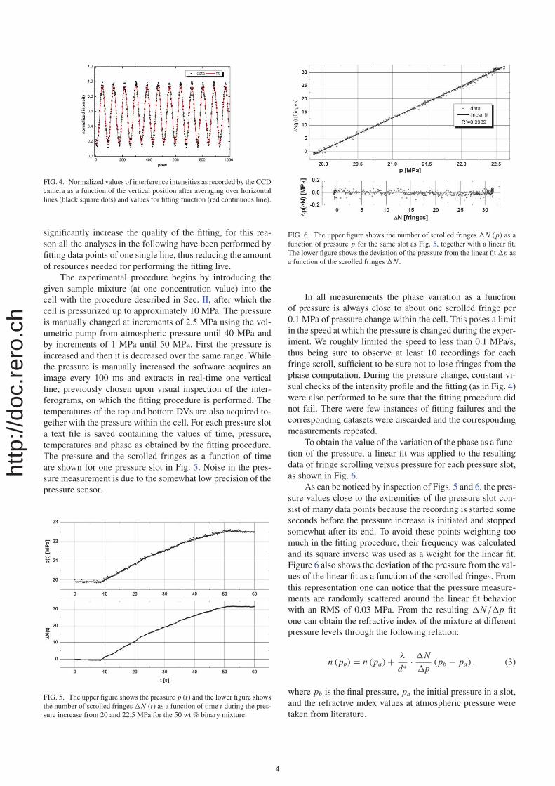
FIG. 4. Normalized values of interference intensities as recorded by the CCDcamera as a function of the vertical position after averaging over horizontallines (black square dots) and values for fitting function (red continuous line).

significantly increase the quality of the fitting, for this rea-son all the analyses in the following have been performed byfitting data points of one single line, thus reducing the amountof resources needed for performing the fitting live.

The experimental procedure begins by introducing thegiven sample mixture (at one concentration value) into thecell with the procedure described in Sec. II, after which thecell is pressurized up to approximately 10 MPa. The pressureis manually changed at increments of 2.5 MPa using the vol-umetric pump from atmospheric pressure until 40 MPa andby increments of 1 MPa until 50 MPa. First the pressure isincreased and then it is decreased over the same range. Whilethe pressure is manually increased the software acquires animage every 100 ms and extracts in real-time one verticalline, previously chosen upon visual inspection of the inter-ferograms, on which the fitting procedure is performed. Thetemperatures of the top and bottom DVs are also acquired to-gether with the pressure within the cell. For each pressure slota text file is saved containing the values of time, pressure,temperatures and phase as obtained by the fitting procedure.The pressure and the scrolled fringes as a function of timeare shown for one pressure slot in Fig. 5. Noise in the pres-sure measurement is due to the somewhat low precision of thepressure sensor.

FIG. 5. The upper figure shows the pressure p (t) and the lower figure showsthe number of scrolled fringes �N (t) as a function of time t during the pres-sure increase from 20 and 22.5 MPa for the 50 wt.% binary mixture.

FIG. 6. The upper figure shows the number of scrolled fringes �N (p) as afunction of pressure p for the same slot as Fig. 5, together with a linear fit.The lower figure shows the deviation of the pressure from the linear fit �p asa function of the scrolled fringes �N .

In all measurements the phase variation as a functionof pressure is always close to about one scrolled fringe per0.1 MPa of pressure change within the cell. This poses a limitin the speed at which the pressure is changed during the exper-iment. We roughly limited the speed to less than 0.1 MPa/s,thus being sure to observe at least 10 recordings for eachfringe scroll, sufficient to be sure not to lose fringes from thephase computation. During the pressure change, constant vi-sual checks of the intensity profile and the fitting (as in Fig. 4)were also performed to be sure that the fitting procedure didnot fail. There were few instances of fitting failures and thecorresponding datasets were discarded and the correspondingmeasurements repeated.

To obtain the value of the variation of the phase as a func-tion of the pressure, a linear fit was applied to the resultingdata of fringe scrolling versus pressure for each pressure slot,as shown in Fig. 6.

As can be noticed by inspection of Figs. 5 and 6, the pres-sure values close to the extremities of the pressure slot con-sist of many data points because the recording is started someseconds before the pressure increase is initiated and stoppedsomewhat after its end. To avoid these points weighting toomuch in the fitting procedure, their frequency was calculatedand its square inverse was used as a weight for the linear fit.Figure 6 also shows the deviation of the pressure from the val-ues of the linear fit as a function of the scrolled fringes. Fromthis representation one can notice that the pressure measure-ments are randomly scattered around the linear fit behaviorwith an RMS of 0.03 MPa. From the resulting �N/�p fitone can obtain the refractive index of the mixture at differentpressure levels through the following relation:

n (pb) = n (pa) + λ

d∗ · �N

�p(pb − pa) , (3)

where pb is the final pressure, pa the initial pressure in a slot,and the refractive index values at atmospheric pressure weretaken from literature.

http

://do

c.re

ro.c

h

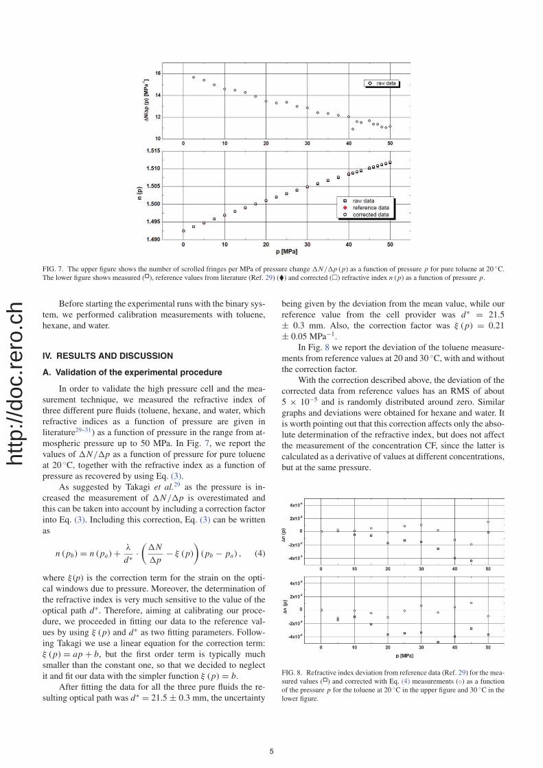
FIG. 7. The upper figure shows the number of scrolled fringes per MPa of pressure change �N/�p (p) as a function of pressure p for pure toluene at 20 ◦C.The lower figure shows measured (�), reference values from literature (Ref. 29) (�) and corrected (�) refractive index n (p) as a function of pressure p.

Before starting the experimental runs with the binary sys-tem, we performed calibration measurements with toluene,hexane, and water.

IV. RESULTS AND DISCUSSION

A. Validation of the experimental procedure

In order to validate the high pressure cell and the mea-surement technique, we measured the refractive index ofthree different pure fluids (toluene, hexane, and water, whichrefractive indices as a function of pressure are given inliterature29–31) as a function of pressure in the range from at-mospheric pressure up to 50 MPa. In Fig. 7, we report thevalues of �N/�p as a function of pressure for pure tolueneat 20 ◦C, together with the refractive index as a function ofpressure as recovered by using Eq. (3).

As suggested by Takagi et al.29 as the pressure is in-creased the measurement of �N/�p is overestimated andthis can be taken into account by including a correction factorinto Eq. (3). Including this correction, Eq. (3) can be writtenas

n (pb) = n (pa) + λ

d∗ ·(

�N

�p− ξ (p)

)(pb − pa) , (4)

where ξ (p) is the correction term for the strain on the opti-cal windows due to pressure. Moreover, the determination ofthe refractive index is very much sensitive to the value of theoptical path d∗. Therefore, aiming at calibrating our proce-dure, we proceeded in fitting our data to the reference val-ues by using ξ (p) and d∗ as two fitting parameters. Follow-ing Takagi we use a linear equation for the correction term:ξ (p) = ap + b, but the first order term is typically muchsmaller than the constant one, so that we decided to neglectit and fit our data with the simpler function ξ (p) = b.

After fitting the data for all the three pure fluids the re-sulting optical path was d∗ = 21.5 ± 0.3 mm, the uncertainty

being given by the deviation from the mean value, while ourreference value from the cell provider was d∗ = 21.5± 0.3 mm. Also, the correction factor was ξ (p) = 0.21± 0.05 MPa−1.

In Fig. 8 we report the deviation of the toluene measure-ments from reference values at 20 and 30 ◦C, with and withoutthe correction factor.

With the correction described above, the deviation of thecorrected data from reference values has an RMS of about5 × 10−5 and is randomly distributed around zero. Similargraphs and deviations were obtained for hexane and water. Itis worth pointing out that this correction affects only the abso-lute determination of the refractive index, but does not affectthe measurement of the concentration CF, since the latter iscalculated as a derivative of values at different concentrations,but at the same pressure.

FIG. 8. Refractive index deviation from reference data (Ref. 29) for the mea-sured values (�) and corrected with Eq. (4) measurements (◦) as a functionof the pressure p for the toluene at 20 ◦C in the upper figure and 30 ◦C in thelower figure.

http

://do

c.re

ro.c

h

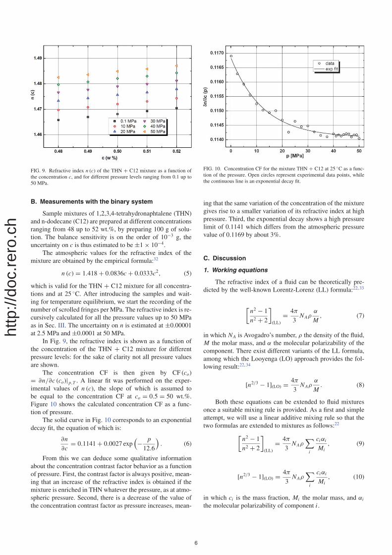
FIG. 9. Refractive index n (c) of the THN + C12 mixture as a function ofthe concentration c, and for different pressure levels ranging from 0.1 up to50 MPa.

B. Measurements with the binary system

Sample mixtures of 1,2,3,4-tetrahydronaphtalene (THN)and n-dodecane (C12) are prepared at different concentrationsranging from 48 up to 52 wt.%, by preparing 100 g of solu-tion. The balance sensitivity is on the order of 10−3 g, theuncertainty on c is thus estimated to be ±1 × 10−4.

The atmospheric values for the refractive index of themixture are obtained by the empirical formula:32

n (c) = 1.418 + 0.0836c + 0.0333c2, (5)

which is valid for the THN + C12 mixture for all concentra-tions and at 25 ◦C. After introducing the samples and wait-ing for temperature equilibrium, we start the recording of thenumber of scrolled fringes per MPa. The refractive index is re-cursively calculated for all the pressure values up to 50 MPaas in Sec. III. The uncertainty on n is estimated at ±0.00001at 2.5 MPa and ±0.0001 at 50 MPa.

In Fig. 9, the refractive index is shown as a function ofthe concentration of the THN + C12 mixture for differentpressure levels: for the sake of clarity not all pressure valuesare shown.

The concentration CF is then given by CF (co)= ∂n/∂c (co)|p,T . A linear fit was performed on the exper-imental values of n (c), the slope of which is assumed tobe equal to the concentration CF at co = 0.5 = 50 wt.%.Figure 10 shows the calculated concentration CF as a func-tion of pressure.

The solid curve in Fig. 10 corresponds to an exponentialdecay fit, the equation of which is:

∂n

∂c= 0.1141 + 0.0027 exp

(− p

12.6

). (6)

From this we can deduce some qualitative informationabout the concentration contrast factor behavior as a functionof pressure. First, the contrast factor is always positive, mean-ing that an increase of the refractive index is obtained if themixture is enriched in THN whatever the pressure, as at atmo-spheric pressure. Second, there is a decrease of the value ofthe concentration contrast factor as pressure increases, mean-

FIG. 10. Concentration CF for the mixture THN + C12 at 25 ◦C as a func-tion of the pressure. Open circles represent experimental data points, whilethe continuous line is an exponential decay fit.

ing that the same variation of the concentration of the mixturegives rise to a smaller variation of its refractive index at highpressure. Third, the exponential decay shows a high pressurelimit of 0.1141 which differs from the atmospheric pressurevalue of 0.1169 by about 3%.

C. Discussion

1. Working equations

The refractive index of a fluid can be theoretically pre-dicted by the well-known Lorentz-Lorenz (LL) formula:22,33

[n2 − 1

n2 + 2

](LL)

= 4π

3NAρ

α

M, (7)

in which NA is Avogadro’s number, ρ the density of the fluid,M the molar mass, and α the molecular polarizability of thecomponent. There exist different variants of the LL formula,among which the Looyenga (LO) approach provides the fol-lowing result:22, 34

[n2/3 − 1](LO) = 4π

3NAρ

α

M. (8)

Both these equations can be extended to fluid mixturesonce a suitable mixing rule is provided. As a first and simpleattempt, we will use a linear additive mixing rule so that thetwo formulas are extended to mixtures as follows:22[

n2 − 1

n2 + 2

](LL)

= 4π

3NAρ

∑i

ciαi

Mi, (9)

[n2/3 − 1](LO) = 4π

3NAρ

∑i

ciαi

Mi, (10)

in which ci is the mass fraction, Mi the molar mass, and αi

the molecular polarizability of component i .

http

://do

c.re

ro.c

h

The concentration CF for a binary mixture with a linearmixing rule can be deduced to be(

∂n

∂c

)p,T (LL)

= (n2 − 1)(n2 + 2)

6n

×[1

ρ

(∂ρ

∂c

)P,T

+α1M1

− α2M2

cα1M1

+ (1−c)α2M2

], (11)

(∂n

∂c

)p,T (LO)

= 3

2(n − n1/3)

×[1

ρ

(∂ρ

∂c

)P,T

+α1M1

− α2M2

cα1M1

+ (1−c)α2M2

], (12)

in which 1/ρ (∂ρ/∂c)P,T = β is the mass expansion coeffi-cient of the mixture.

Two kind of comparison can be performed to validateour measurements. First, one can compare the left hands ofEqs. (9) and (10) (with the experimental values of n) withthe corresponding right hands of the respective equations, inorder to check the measured values of the refractive index nagainst the two different theoretical approaches. Second, onecan compare the left hands of Eqs. (11) and (12) (with themeasured values of the concentration CF) against the righthands of the same formulas. In this way, a check of the con-centration CF against the two theories is obtained. In order toperform these comparisons one needs to know the values ofthe molecular polarizability of the two molecules as well asthe density and the mass expansion coefficient of the mixtureas a function of the pressure. While the latter have been mea-sured by some of us in a previous experiment,35 the formeris not easy to measure and there exist no reference value inliterature for the two components of choice at high pressure.

In order to obtain the polarizability, quantum calcula-tions have been performed as detailed in the Appendix. Es-sentially these calculations showed a marginal dependence of

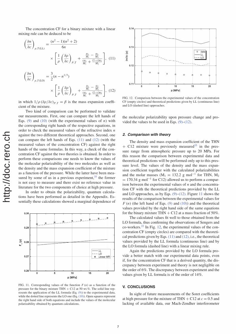
FIG. 11. Corresponding values of the function F (n) as a function of thepressure for the binary mixture THN + C12 at 50 wt.%. The solid line rep-resents the application of the LL formula (Eq. (9)) to the experimental data,while the dotted line represents the LO one (Eq. (10)). Open squares representthe right hand side of both equations and include the values of the molecularpolarizability obtained by quantum calculations.

FIG. 12. Comparison between the experimental values of the concentrationCF (empty circles) and theoretical predictions given by LL (continuous line)and LO (dashed line) approaches.

the molecular polarizability upon pressure change and pro-vided the values to be used in Eqs. (9)–(12).

2. Comparison with theory

The density and mass expansion coefficient of the THN+ C12 mixture were previously measured35 in the pres-sure range from atmospheric pressure up to 20 MPa. Forthis reason the comparison between experimental data andtheoretical predictions will be performed only up to this pres-sure level. The values of the density and the mass expan-sion coefficient together with the calculated polarizabilitiesand the molar masses (M1 = 132.2 g mol−1 for THN, M2

= 170.34 g mol−1 for C12) allowed us to perform a compar-ison between the experimental values of n and the concentra-tion CF with the theoretical predictions provided by the LLand LO approaches, as by Eqs. (9)–(12). Figure 11 shows theresults of the comparison between the experimental values forF (n) (the left hand of Eqs. (9) and (10)) and the theoreticalvalues provided by the right hand side of the same equationsfor the binary mixture THN + C12 at a mass fraction of 50%.

The calculated values fit well to those obtained from theLO formula, thus confirming the observations of Sengers andco-workers.22 In Fig. 12, the experimental values of the con-centration CF (empty circles) are compared with the theoreti-cal predictions given by Eqs. (11) and (12), i.e., the theoreticalvalues provided by the LL formula (continuous line) and bythe LO formula (dashed line) with a linear mixing rule.

Again the predictions provided by the LO formula pro-vide a better match with our experimental data points, evenif, for the concentration CF that is a derived quantity, the dis-crepancy between experiment and theory is not negligible onthe order of 6%. The discrepancy between experiment and thevalues given by LL formula is of the order of 14%.

V. CONCLUSIONS

In sight of future measurements of the Soret coefficientsat high pressure for the mixture of THN + C12 at c = 0.5 andlacking of available data, our Mach-Zendher interferometer

http

://do

c.re

ro.c

h

has been modified to measure the concentration contrast fac-tor (∂n/∂c)P,T at different pressures in the range between at-mospheric pressure and 50MPa. Measurements demonstratedan exponential decay in the concentration CF with pressurein the pressure range under investigation for this mixture. Acomparison with theory required the calculation of the twomolecules polarizabilities as a function of pressure. The com-parison between our experimental results of n and the concen-tration CF with the results provided by Lorentz-Lorenz andLooyenga formulas extended to binaries with a linear mixingrule showed very good agreement with the Looyenga formulafor the refractive index and a certain agreement with the de-duced expression of concentration CF.

ACKNOWLEDGMENTS

This work was financially supported by the EuropeanSpace Agency and the PRES of Bordeaux. Ian Block is grate-fully thanked for critically revising the paper. F.C. acknowl-edges present support from the European Union under MarieCurie funding, contract No. IEF-251131, DyNeFI Project.

APPENDIX: POLARIZABILITY QUANTUMCALCULATIONS

Ab initio calculations of (hyper)polarizabilities are nowa-days of routine for molecular systems into gas phase, i.e.,isolated systems.36 Theoretical studies concerning manymolecular systems developed with the help of analytical ornumerical approaches is prolix in this field. So, it is not sur-prising to find theoretical data on systems studied in thiswork.37 Nevertheless, pressure information is not availableand models are generally not adapted to take into account thisparameter. Automatic algorithms devoted to the calculation oflocal properties like individual polarizability under pressuremust then be developed as detailed in the following.

Different configurations of the isolated and/or embed-ded THN and C12 fluids have been tested, the environmen-tal effects such as pressure and interaction energies beingkey parameters in explaining the refractive index dependence,shown in the LL or LO formulas. Ab initio calculations wereapplied by using the 6-311+G** basis set.38 The method usedwas the density functional theory (DFT), namely wB97XD(Ref. 39) including a long-range corrected hybrid densityfunctional with damped atom-atom dispersion corrections.Optimized geometries, energies, and analytical first deriva-tives were obtained with the GAUSSIAN 09 package.40 Zero-

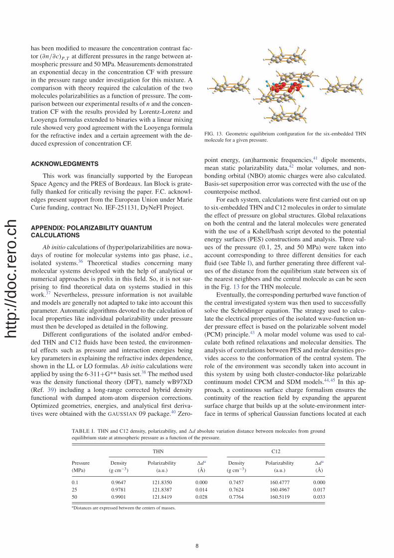
FIG. 13. Geometric equilibrium configuration for the six-embedded THNmolecule for a given pressure.

point energy, (an)harmonic frequencies,41 dipole moments,mean static polarizability data,42 molar volumes, and non-bonding orbital (NBO) atomic charges were also calculated.Basis-set superposition error was corrected with the use of thecounterpoise method.

For each system, calculations were first carried out on upto six-embedded THN and C12 molecules in order to simulatethe effect of pressure on global structures. Global relaxationson both the central and the lateral molecules were generatedwith the use of a Kshell/bash script devoted to the potentialenergy surfaces (PES) constructions and analysis. Three val-ues of the pressure (0.1, 25, and 50 MPa) were taken intoaccount corresponding to three different densities for eachfluid (see Table I), and further generating three different val-ues of the distance from the equilibrium state between six ofthe nearest neighbors and the central molecule as can be seenin the Fig. 13 for the THN molecule.

Eventually, the corresponding perturbed wave function ofthe central investigated system was then used to successfullysolve the Schrödinger equation. The strategy used to calcu-late the electrical properties of the isolated wave-function un-der pressure effect is based on the polarizable solvent model(PCM) principle.43 A molar model volume was used to cal-culate both refined relaxations and molecular densities. Theanalysis of correlations between PES and molar densities pro-vides access to the conformation of the central system. Therole of the environment was secondly taken into account inthis system by using both cluster-conductor-like polarizablecontinuum model CPCM and SDM models.44, 45 In this ap-proach, a continuous surface charge formalism ensures thecontinuity of the reaction field by expanding the apparentsurface charge that builds up at the solute-environment inter-face in terms of spherical Gaussian functions located at each

TABLE I. THN and C12 density, polarizability, and �d absolute variation distance between molecules from groundequilibrium state at atmospheric pressure as a function of the pressure.

THN C12

Pressure Density Polarizability �da Density Polarizability �da

(MPa) (g cm−3) (a.u.) (Å) (g cm−3) (a.u.) (Å)

0.1 0.9647 121.8350 0.000 0.7457 160.4777 0.00025 0.9781 121.8387 0.014 0.7624 160.4967 0.01750 0.9901 121.8419 0.028 0.7764 160.5119 0.033

aDistances are expressed between the centers of masses.

http

://do

c.re

ro.c

h

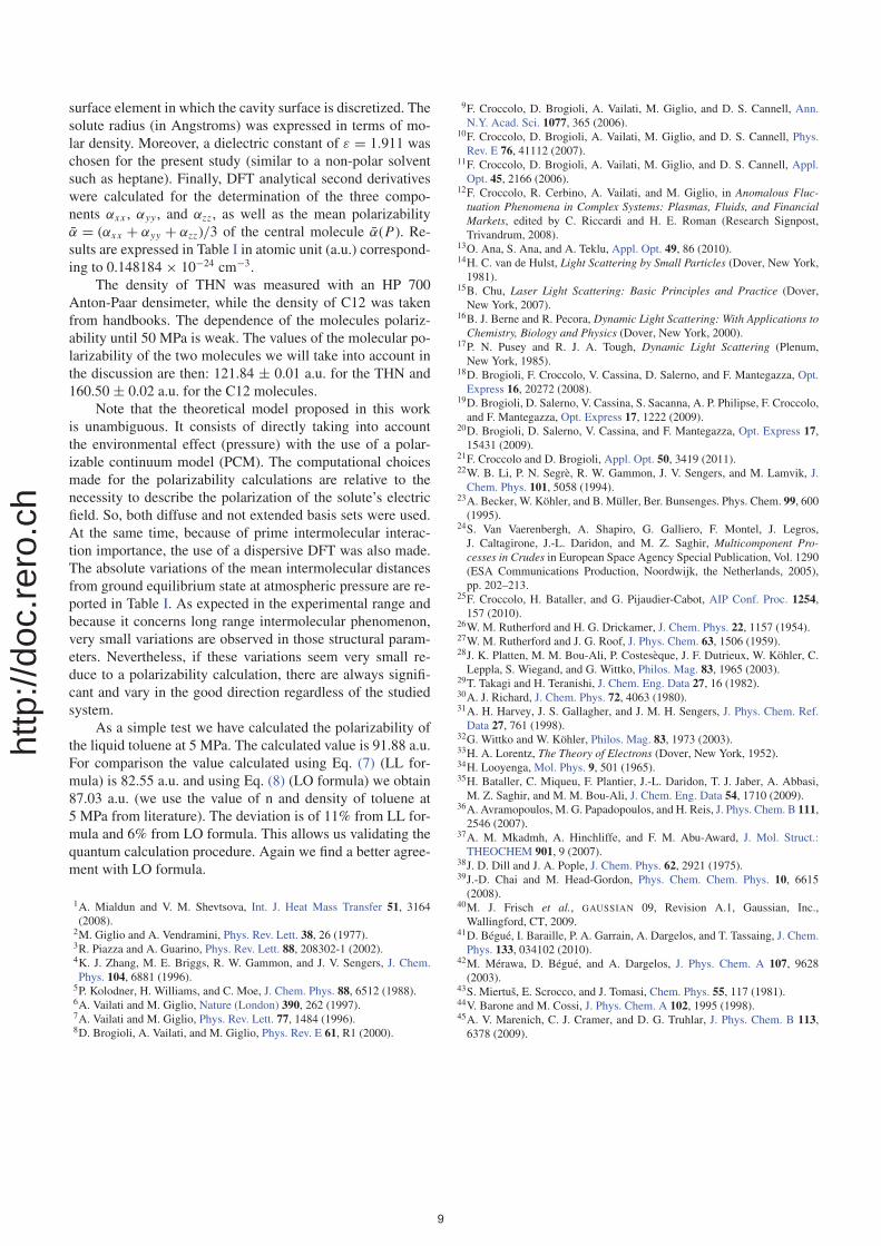
surface element in which the cavity surface is discretized. Thesolute radius (in Angstroms) was expressed in terms of mo-lar density. Moreover, a dielectric constant of ε = 1.911 waschosen for the present study (similar to a non-polar solventsuch as heptane). Finally, DFT analytical second derivativeswere calculated for the determination of the three compo-nents αxx , αyy , and αzz , as well as the mean polarizabilityα = (αxx + αyy + αzz)/3 of the central molecule α(P). Re-sults are expressed in Table I in atomic unit (a.u.) correspond-ing to 0.148184 × 10−24 cm−3.

The density of THN was measured with an HP 700Anton-Paar densimeter, while the density of C12 was takenfrom handbooks. The dependence of the molecules polariz-ability until 50 MPa is weak. The values of the molecular po-larizability of the two molecules we will take into account inthe discussion are then: 121.84 ± 0.01 a.u. for the THN and160.50 ± 0.02 a.u. for the C12 molecules.

Note that the theoretical model proposed in this workis unambiguous. It consists of directly taking into accountthe environmental effect (pressure) with the use of a polar-izable continuum model (PCM). The computational choicesmade for the polarizability calculations are relative to thenecessity to describe the polarization of the solute’s electricfield. So, both diffuse and not extended basis sets were used.At the same time, because of prime intermolecular interac-tion importance, the use of a dispersive DFT was also made.The absolute variations of the mean intermolecular distancesfrom ground equilibrium state at atmospheric pressure are re-ported in Table I. As expected in the experimental range andbecause it concerns long range intermolecular phenomenon,very small variations are observed in those structural param-eters. Nevertheless, if these variations seem very small re-duce to a polarizability calculation, there are always signifi-cant and vary in the good direction regardless of the studiedsystem.

As a simple test we have calculated the polarizability ofthe liquid toluene at 5 MPa. The calculated value is 91.88 a.u.For comparison the value calculated using Eq. (7) (LL for-mula) is 82.55 a.u. and using Eq. (8) (LO formula) we obtain87.03 a.u. (we use the value of n and density of toluene at5 MPa from literature). The deviation is of 11% from LL for-mula and 6% from LO formula. This allows us validating thequantum calculation procedure. Again we find a better agree-ment with LO formula.

1A. Mialdun and V. M. Shevtsova, Int. J. Heat Mass Transfer 51, 3164(2008).

2M. Giglio and A. Vendramini, Phys. Rev. Lett. 38, 26 (1977).3R. Piazza and A. Guarino, Phys. Rev. Lett. 88, 208302-1 (2002).4K. J. Zhang, M. E. Briggs, R. W. Gammon, and J. V. Sengers, J. Chem.Phys. 104, 6881 (1996).

5P. Kolodner, H. Williams, and C. Moe, J. Chem. Phys. 88, 6512 (1988).6A. Vailati and M. Giglio, Nature (London) 390, 262 (1997).7A. Vailati and M. Giglio, Phys. Rev. Lett. 77, 1484 (1996).8D. Brogioli, A. Vailati, and M. Giglio, Phys. Rev. E 61, R1 (2000).

9F. Croccolo, D. Brogioli, A. Vailati, M. Giglio, and D. S. Cannell, Ann.N.Y. Acad. Sci. 1077, 365 (2006).

10F. Croccolo, D. Brogioli, A. Vailati, M. Giglio, and D. S. Cannell, Phys.Rev. E 76, 41112 (2007).

11F. Croccolo, D. Brogioli, A. Vailati, M. Giglio, and D. S. Cannell, Appl.Opt. 45, 2166 (2006).

12F. Croccolo, R. Cerbino, A. Vailati, and M. Giglio, in Anomalous Fluc-tuation Phenomena in Complex Systems: Plasmas, Fluids, and FinancialMarkets, edited by C. Riccardi and H. E. Roman (Research Signpost,Trivandrum, 2008).

13O. Ana, S. Ana, and A. Teklu, Appl. Opt. 49, 86 (2010).14H. C. van de Hulst, Light Scattering by Small Particles (Dover, New York,1981).

15B. Chu, Laser Light Scattering: Basic Principles and Practice (Dover,New York, 2007).

16B. J. Berne and R. Pecora, Dynamic Light Scattering: With Applications toChemistry, Biology and Physics (Dover, New York, 2000).

17P. N. Pusey and R. J. A. Tough, Dynamic Light Scattering (Plenum,New York, 1985).

18D. Brogioli, F. Croccolo, V. Cassina, D. Salerno, and F. Mantegazza, Opt.Express 16, 20272 (2008).

19D. Brogioli, D. Salerno, V. Cassina, S. Sacanna, A. P. Philipse, F. Croccolo,and F. Mantegazza, Opt. Express 17, 1222 (2009).

20D. Brogioli, D. Salerno, V. Cassina, and F. Mantegazza, Opt. Express 17,15431 (2009).

21F. Croccolo and D. Brogioli, Appl. Opt. 50, 3419 (2011).22W. B. Li, P. N. Segrè, R. W. Gammon, J. V. Sengers, and M. Lamvik, J.Chem. Phys. 101, 5058 (1994).

23A. Becker, W. Köhler, and B. Müller, Ber. Bunsenges. Phys. Chem. 99, 600(1995).

24S. Van Vaerenbergh, A. Shapiro, G. Galliero, F. Montel, J. Legros,J. Caltagirone, J.-L. Daridon, and M. Z. Saghir, Multicomponent Pro-cesses in Crudes in European Space Agency Special Publication, Vol. 1290(ESA Communications Production, Noordwijk, the Netherlands, 2005),pp. 202–213.

25F. Croccolo, H. Bataller, and G. Pijaudier-Cabot, AIP Conf. Proc. 1254,157 (2010).

26W. M. Rutherford and H. G. Drickamer, J. Chem. Phys. 22, 1157 (1954).27W. M. Rutherford and J. G. Roof, J. Phys. Chem. 63, 1506 (1959).28J. K. Platten, M. M. Bou-Ali, P. Costesèque, J. F. Dutrieux, W. Köhler, C.Leppla, S. Wiegand, and G. Wittko, Philos. Mag. 83, 1965 (2003).

29T. Takagi and H. Teranishi, J. Chem. Eng. Data 27, 16 (1982).30A. J. Richard, J. Chem. Phys. 72, 4063 (1980).31A. H. Harvey, J. S. Gallagher, and J. M. H. Sengers, J. Phys. Chem. Ref.Data 27, 761 (1998).

32G. Wittko and W. Köhler, Philos. Mag. 83, 1973 (2003).33H. A. Lorentz, The Theory of Electrons (Dover, New York, 1952).34H. Looyenga, Mol. Phys. 9, 501 (1965).35H. Bataller, C. Miqueu, F. Plantier, J.-L. Daridon, T. J. Jaber, A. Abbasi,M. Z. Saghir, and M. M. Bou-Ali, J. Chem. Eng. Data 54, 1710 (2009).

36A. Avramopoulos, M. G. Papadopoulos, and H. Reis, J. Phys. Chem. B 111,2546 (2007).

37A. M. Mkadmh, A. Hinchliffe, and F. M. Abu-Award, J. Mol. Struct.:THEOCHEM 901, 9 (2007).

38J. D. Dill and J. A. Pople, J. Chem. Phys. 62, 2921 (1975).39J.-D. Chai and M. Head-Gordon, Phys. Chem. Chem. Phys. 10, 6615(2008).

40M. J. Frisch et al., GAUSSIAN 09, Revision A.1, Gaussian, Inc.,Wallingford, CT, 2009.

41D. Bégué, I. Baraille, P. A. Garrain, A. Dargelos, and T. Tassaing, J. Chem.Phys. 133, 034102 (2010).

42M. Mérawa, D. Bégué, and A. Dargelos, J. Phys. Chem. A 107, 9628(2003).

43S. Miertuš, E. Scrocco, and J. Tomasi, Chem. Phys. 55, 117 (1981).44V. Barone and M. Cossi, J. Phys. Chem. A 102, 1995 (1998).45A. V. Marenich, C. J. Cramer, and D. G. Truhlar, J. Phys. Chem. B 113,6378 (2009).

http

://do

c.re

ro.c

h