Concentration dependence of fluorescence quenching by ionic reactants

INSTITUTE OF PHYSICS PUBLISHING JOURNAL OF PHYSICS: CONDENSED MATTER

J. Phys.: Condens. Matter 19 (2007) 065111 (14pp) doi:10.1088/0953-8984/19/6/065111

Concentration dependence of fluorescence quenching

by ionic reactants

Sergey D Traytak1 and Masanori Tachiya

National Institute of Advanced Industrial Science and Technology (AIST), 1-1-1 Higashi,

Tsukuba, Ibaraki 305-8565, Japan

E-mail: [email protected] and [email protected]

Received 7 August 2006, in final form 25 September 2006

Published 22 January 2007

Online at stacks.iop.org/JPhysCM/19/065111

Abstract

Fluorescence quenching for ionic reactants when the quenchers are nondilute

is studied theoretically. The fluorophore and quenchers are assumed to interact

by Coulomb potential. It has been shown that for oppositely charged ions with

large Onsager length the positive deviation from the linear Stern–Volmer law is

negligibly small. Our results are in good agreement with available experimental

data on the luminescence quenching of the ions W6I2−14 by bipyridinium ions.

1. Introduction

Fluorescence quenching in solution is a simple example of diffusion-controlled reaction of the

pseudo first-order

A + B∗ → A + B,

where A is a quencher, B and B∗ are the ground and an excited state of the fluorophore [1].

Hereafter we assume that both species have spherically symmetric reactivity. Since the

quencher concentration c is a constant, we can consider quenchers as sinks of infinite capacity.

It is well-known that the lifetime τ of an excited fluorophore in solution containing

quenchers obeys the relation [1, 2]

1

τ=

1

τ0

+ kc, (1)

where τ0 is the intrinsic lifetime of the fluorophore in the absence of quenchers and kc is the

rate coefficient for quenching. Thus the intrinsic lifetime of the fluorophore is shortened due to

the presence of quenchers. To calculate kc it is convenient to assume that fluorophore reactants

diffuse towards immobile sinks with a relative diffusion coefficient. For instance, in the case

1 Permanent address: Institute of Applied Mechanics of the Russian Academy of Sciences, 32-a Lenin Avenue,

Moscow 117334, Russia.

0953-8984/07/065111+14$30.00 © 2007 IOP Publishing Ltd Printed in the UK 1

J. Phys.: Condens. Matter 19 (2007) 065111 S D Traytak and M Tachiya

of uncharged reactants and fully diffusion-controlled quenching at very low concentrations of

quenchers, one can use the Smoluchowski steady-state rate coefficient [3]

kS = 4π DR, (2)

where D = DA + DB , DA and DB are the diffusion coefficients of quencher and fluorophore,

respectively; R is the encounter distance. Thus in this case ignoring the time-dependent effects

we have the classical linear Stern–Volmer law [4, 2, 5]

I0

I (c)= 1 + kScτ0, (3)

where I0 and I (c) are the fluorescence intensity in the absence and in the presence of quenchers,

respectively.

However, at higher quencher concentrations the problem of concentration effects naturally

arises, and we cannot find the value of kc by simple multiplying kS by the quencher

concentration c. In the case of uncharged reactants, Felderhof and Deutch [6], and

independently Brailsford [7], showed that the first correction to the steady-state reaction rate in

terms of the concentration has a nonanalytical behaviour

k(c) = kS

(1 +

√3φ + · · ·

), (4)

where φ = 4π R3c/3 is the material volume fraction of the total volume occupied by sinks

(quenchers). Since these pioneering works, several theories of the concentration dependence of

the rate coefficient have been proposed [1, 2, 8, 9]. It has been shown that for the fluorescence

quenching the concentration dependence leads to positive deviation from the Stern–Volmer

law [10–13].

Theoretical studies of the concentration dependence in the case of reactants which are

subjected to the influence of a dynamical potential are very few. In a series of papers [14–16]

using both the mean field approach and the effective medium theory, Cukier came to the

conclusion that for ionic reactions the structure of the concentration dependence remains the

same as in the case of neutral reactants, equation (4), but with renormalized value of φ, i.e.

k(c) = kD

(1 +

√3φ + · · ·

), (5)

where φ = 4π R3c/3 is the so-called effective volume fraction and R is the effective radius

defined by the Debye formula for the steady-state rate coefficient in the case of the Coulomb

interaction potential [17]

kD = 4π DR, i.e. R = −α∗

1 − eα∗ R. (6)

Here α∗ = α/R, α = z AzBrc, with the Onsager length rc = βe2/4πεε0; z Ae and zBe are

the charges of sink and fluorophore, respectively; e is the electronic charge; ε and ε0 are the

dielectric constant of the solution and free space, respectively; β = 1/kBT , where kB is the

Boltzmann’s constant and T is the absolute temperature. One can see that in the case of strong

attractive Coulomb potential the magnitude of R becomes much larger than the reaction radius

R (e.g. in cyclohexane R/R ≃ 40) and, therefore, even for small material volume fraction φ

the effective volume fraction φ attains large values. Thus, according to Cukier’s theory, the

long-range attractive potential causes the dramatic concentration effects and leads to nonlinear

Stern–Volmer relation even for low sink concentrations. On the other hand, in the case of a

repulsive potential the situation is opposite and we can ignore the concentration effects for the

strong repulsion.

2

J. Phys.: Condens. Matter 19 (2007) 065111 S D Traytak and M Tachiya

One can see that the concentration dependence is due to the diffusive interaction

(competition) for diffusing reactants. That is the reason why we investigated analytically [18]

and numerically [19] the relatively simple problem on diffusive interaction between two static

charged sinks. It was shown there that for unlike charged particles at large enough values of

the Onsager length the diffusive interaction is negligibly small. It is worth noting that a similar

problem occurs if we treat the electron reactions with the positive ions when the solution of the

latter is not dilute [15]. Obviously this case is a special one of τ0 → ∞ in the above example

and so we will treat here only the case of quenching.

The main purpose of the present paper is to treat concentration effects in nondilute

systems of charged reactants interacting by Coulomb potential for the model of quenching

by immobile sinks. This paper is organized as follows. In section 2 we consider the mean field

approach within the framework of the so-called tilde space method [20]. Section 3 contains

some application of the time-dependent solution of the Debye–Smoluchowski equation to the

problem at issue. In section 4 we present discussion of results obtained and compare them with

known experimental data on the luminescence quenching of ions W6I2−14 by bipyridinium ions.

The main conclusions of the paper are given in the last section 5.

2. Mean field approach

2.1. Statement of the problem

It is well-known that the deviation of the fluorophore local concentration nB(r) from its bulk

value is the largest for totally diffusion-controlled reactions [1, 14, 16]. Thus to assess the

maximum effects of concentration on the linear Stern–Volmer law we restrict our calculation to

the fully diffusion-controlled limit, i.e. we will use the Smoluchowski boundary condition. It is

worth noting here that the result for the Smoluchowski boundary condition may be immediately

generalized to the case of the Collins–Kimball one [21, 22], if we take into account the

connection between the relevant solutions for the time-dependent boundary-value problems

(see section 3).

The mean field approach (MFA) [1, 14, 16, 23] is a well-known and simple method to

calculate the first correction to the concentration dependence of the rate coefficient. We assume

that the characteristic relaxation time is small, and consider the steady-state problem (see

section 4). It is worth noting that the reaction-induced fluctuations in the reactant densities

make the reaction rate time-dependent at all reaction times, although it is not known how

big this effect is under given conditions (initial defect densities, observation times, etc) (see,

e.g. [24] and references therein). The mean field equation is described in terms of the deviation

of the fluorophore local concentration nB(r) from its bulk value n0 about a test quencher:

n(r) = n0 − nB(r). So the function n(r) describes the local inhomogeneity in the vicinity

of the test quencher and obeys the following equation

D∇(∇n + n∇βU) = ksscn + τ−10 n, (7)

where the second term on the right-hand side describes the nonreactive decay due to the intrinsic

lifetime of the fluorophore. The value of the rate coefficient kss should be found with the aid

of some self-consistent procedure given below. We supplement equation (7) with the boundary

condition and condition at infinity

n|r=R = n0, n|r→∞ → 0. (8)

One can see that the boundary condition (8) corresponds to the Smoluchowski condition as

regards nB(r). Further we set τ0 → ∞ for the sake of simplicity.

3

J. Phys.: Condens. Matter 19 (2007) 065111 S D Traytak and M Tachiya

According to the MFA we should equate the appropriate rate coefficient determined by the

equations (7), (8) to the rate coefficient kss on the right-hand side of equation (7), i.e.

−4π DR2 1

n0

dn

dr

∣∣∣∣r=R

= kss . (9)

Equations (7) and (9) indicate that kss is a function of ckss and α and so we assume the existence

of the fixed point of the dependence ckss(ckss; α), i.e.

ckss(ckss; α) = ckss (10)

with the normalization condition kss|c=0 = kD.

In order to obtain the first correction to the rate constant Cukier used an approximate

tilde space method suggested by Flannery [20] for the time-dependent Debye–Smoluchowski

equation (DSE) with a Coulomb potential. Following Flannery he assumed that the tilde space

time-dependent solution works well for all times and, therefore, in the case at issue it is valid

for all values kssc.

2.2. Tilde space method

To compare our consideration with that done in other works [14–16] it is useful to rewrite

equation (7) in the form

D∇ · e−βU ∇eβU n = ksscn. (11)

It was shown in [20] that after the transformation to the so-called ‘tilde’ space

r → r(r) =[∫ ∞

r

1

ξ 2eβU(ξ)dξ

]−1

, n(r) → n(r) = n(r)eβU(r) (12)

we can formally reduce the differential operator in equation (11) to the form of the ‘free’

diffusion equation

DeβU ∇ · e−βU ∇eβU n = D (r) ∇2r n. (13)

Here D(r) = D(dr/dr)2 is a space dependent effective ‘diffusion’ coefficient, where

dr

dr=

(r

r

)2

eβU (14)

and particularly for the Coulomb potential we have

r =α

exp(

α∗

x

)− 1

,dr

dr=

(α∗/x)2

[exp

(α∗

x

)− 1

]2exp

(α∗

x

), (15)

hereafter x = r/R.

To solve the equations (7), (8) analytically following [20], it was assumed in works [14–16]

that

dr/dr = 1. (16)

It is important to note that for solution of the posed problem we need to have a uniform

approximation of the equation at issue for the whole domain of its determination. One can see

from (15) that in the case of Coulomb potential the condition (16) leads to the transcendental

equation

z = sinh z, (17)

where z = r∗c /2x , r∗

c = rc/R. Equation (17) has the only solution z = 0, i.e. it holds either

at r∗c = 0 or in the limit x → ∞ when r∗

c �= 0 is fixed. Nevertheless, we can assume that

4

J. Phys.: Condens. Matter 19 (2007) 065111 S D Traytak and M Tachiya

dr/dr ≈ 1 in the whole domain of determination, when 0.5r∗c ≪ 1, i.e. asymptotically for

very small values of the Onsager length. This is a quite severe restriction of the ‘tilde’ method

(see [25] for details).

Within the framework of the ‘tilde’ method equation (11) under the boundary

conditions (8) may be approximately reduced to the following equation

D∇2r n = ksscn, (18)

and boundary conditions

n|r=R = n0eβU(R), n|r→∞ = 0. (19)

It is well-known that the solution of this problem is

n = n0eβU(R) R

rexp

[−

√ckss

D

(r − R

)]

(20)

and the relevant rate coefficient (9) reads

kss = − 4π DR2 1

n0

d

dr

(e−βU n

)∣∣∣∣r=R

.

Performing simple calculations one gets

kss = 4π DR(α)

[1 +

√ckss

DR(α)eα∗

]. (21)

It is interesting to note that the structure of the concentration correction accurate to the sign is

the same as in formula (37) of [18] for the diffusive interaction between two charged sinks. It

may be shown that this is the exact asymptotic of the rate constant as ckss/D → 0.

One can see that equations (7), (8) are formally identical with the equations satisfied by the

recombination probability of a geminate ion pair interacting through a Coulomb potential with

opposite sign in the presence of scavengers [26]. Thus using the result of [26] we can represent

the exact solution to the boundary-value problem (7), (8) and when ckss is sufficiently small

this taking into account (9) leads also to expression (21).

After the first iteration in (21) in terms of the effective volume fraction φ we readily obtain

kss = 4π DR(α)

(1 +

√3φeα∗

)as c → 0. (22)

This equation is different by a factor of eα∗from the similar result obtained in [14–16].

Let us show that the recent Gopich–Berezhkovskii–Szabo theory [27] and the earlier works

of Richards [28, 29] also leads to the same result. According to this theory,

(c k)−1 ∼∫ ∞

0

dt exp

(−c

∫ t

0

k1

(t ′) dt ′

), as c → 0, (23)

where k1(t) is the time-dependent rate coefficient for a single sink. In the case of an attractive

Coulomb potential the exact long time asymptotic is given by [30, 31]

k1(t) ∼ kD

(1 +

Reα∗

√π Dt

). (24)

Taking equation (24) into account, one can find the integral in (23) as follows:∫ ∞

0

dt exp

(−c

∫ t

0

k1(t′) dt ′

)= (ckD)−1

(1 −

√π ζ eζ 2

erfc ζ)

,

where

ζ =√

3

πφ eα∗

.

Thus for small concentrations expression (23) again yields formula (22).

5

J. Phys.: Condens. Matter 19 (2007) 065111 S D Traytak and M Tachiya

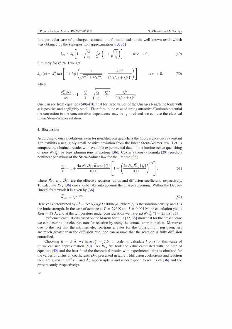
2.3. Cukier’s calculation

Since it has turned out that the use of the same approach leads to different results, now we will

re-examine the derivation given by Cukier [14–16]. In these papers the local concentration was

transformed as follows:

nB(r) = nB(r)eβU(r) (25)

then the following function was introduced

δn = n0 − nB . (26)

For this function the following boundary-value problem was considered [14, 16]

D∇2r δn = ksscδn, δn|r=R = n0, δn|r→∞ = 0. (27)

Thus, by modifying (20) for the given boundary condition one has

δn = n0

R

rexp

[−

√ckss

D

(r − R

)]

,

and the corresponding rate coefficient is given by

kss = −4π DR2 1

n0

dδn

dr

∣∣∣∣r=R

= R(α)

[1 +

√ckss

DR(α)

](28)

or

kss = 4π DR(α)

(1 +

√3φ

). (29)

However this result is not valid for the problem at issue. It is evident that

D∇ · e−βU ∇eβU n0 = n0β∇2U

and therefore for the case of Coulomb potential we have

D∇ · e−βU ∇eβU (n0 − nB) = −D∇ · e−βU ∇eβU nB

= D∇ · e−βU ∇(n0 − eβU nB

)= D∇ · e−βU ∇δn.

After the tilde transformation r → r using (14) we get

D∇ · e−βU ∇δn = DeβU

(r

r

)4

∇2r δn = De−βU

(dr

dr

)2

∇2r δn.

Setting then dr/dr = 1 we arrive at

D∇2r δn = kssceβU (n0 − nB) �= ksscδn.

Thus substitution (26) does not lead to the first equation in (27).

Direct calculation shows that equation (29) may be obtained provided one uses the function

δn = n0e−βU − nB. It means that in equation (7) the deviation from the local Boltzmann’s

distribution was considered, although it is claimed in [14, 16] that the deviation from the bulk

concentration n0 is considered. To compare with analytical results, the numerical solution was

performed in [16]. However, instead of the deviation of the local concentration from its bulk

value, i.e. n = n0 − nB the deviation from its equilibrium value n0e−βU − nB was considered

in the numerical calculations as well. So good agreement obtained there between numerical

results and analytical formula for small concentration c is not surprising.

6

J. Phys.: Condens. Matter 19 (2007) 065111 S D Traytak and M Tachiya

3. MFA and subsidiary time-dependent problem

3.1. Subsidiary time-dependent problem

As shown in [1], the problem at issue is related to a time-dependent boundary-value problem

for the DSE with Coulomb potential. The boundary-value problems for the DSE are well

investigated (see [25] and references therein), and therefore it is convenient to reduce the

original problem to a corresponding subsidiary one.

Let us consider the following subsidiary initial boundary-value problem for the DSE with

a Coulomb potential

∂ρ

∂ t=

(2

x−

α∗

x2

)∂ρ

∂x+

∂2ρ

∂x2, (30)

ρ|t=0 = 0, ρ|x=1 = 1, ρ|x→∞ → 0, (31)

where ρ = 1 − ρB/ρ0 and ρB(x, t) is the local time-dependent concentration of excited ions

B∗ around a test ion quencher A with the random initial distribution ρB |t=0 = ρ0 and the

Smoluchowski boundary condition. Hereafter t is the dimensionless time normalized by the

characteristic relaxation time for pure diffusion td = R2/D. As it was noted in [1] the mean

field boundary-value problem (7), (8) is formally identical with the Laplace–Carson transform

of the initial boundary-value problem (30) and (31), i.e.

d2ρ

dx2+

(2

x−

α∗

x2

)dρ

dx= λρ, (32)

ρ|x=1 = 1, ρ|x→∞ → 0. (33)

Here

ρ (x; λ) =∫ ∞

0

λρ(x, t)e−λt dt, λ = td(kssc + τ−1

0

). (34)

Contrary to the standard Laplace–Carson transform, we assume λ to be a positive real number.

It is evident that

k(λ; α) =∫ ∞

0

λk(t; α)e−λt dt = −dρ

dx

∣∣∣∣x=1

is the corresponding λ-transformed time-dependent reduced rate coefficient. Thus using the

mean field self-consistency condition we have [1]

kss(c) = kS k (λ; α)∣∣λ=td(kss c+τ−1

0 ). (35)

Consider now some important properties of the exact solution.

Property 1. One can show directly or using results of [31] that

ρ (x, λ; α) = exp

[α∗

(1 −

1

x

)]ρ (x, λ; −α) , (36)

k (λ; α) = −α∗ + k (λ; −α) . (37)

These relationships are exact, so if we know functions ρ(x, λ; α) and k(λ; α) for the case of

attraction potential α < 0 we can calculate them for the case of repulsion.

Taking this property into account hereafter we restrict ourselves only to the case of

attractive potential.

7

J. Phys.: Condens. Matter 19 (2007) 065111 S D Traytak and M Tachiya

Property 2. Let functions wl(x, t) and wu(x, t) be the uniform lower and upper boundaries for

ρ(x, t) when x � 1, t � 0, i.e. wl(x, t) � ρ(x, t) � wu(x, t) then one can readily show that

the following relations hold

wl (x; λ) � ρ (x; λ) � wu (x; λ) . (38)

For the corresponding rate constants one has kl(t) � k(t) � ku(t), t > 0, and therefore

k l(λ) � k(λ) � ku(λ) for all λ > 0. (39)

Inequalities (38) and (39) are useful for deriving approximations for the exact solution and

corresponding rate coefficients.

3.2. Approximations for the rate constant

The exact analytical solution of the boundary-value problem (32) and (33) is known [32, 33].

However, it is represented in a very cumbersome form which, except for the case of very

small values of λ or the Onsager length r∗c , renders practical calculations difficult. The

most interesting physical result was predicted just for the large values of the Onsager length

r∗c [14–16] and this very case may be studied by the singular perturbation method [31]. It was

shown that for the DSE with the attractive Coulomb potential and the random initial condition,

the reduced time-dependent rate constant is approximated by the expression

kas(t; r∗c ) =

(1 +

1√

π t

)e− 1

4r∗2

c t +r∗

c

2

[1 + erf

(r∗

c

2

√t

)]. (40)

This formula gives the correct asymptotics in the cases: (a) as r∗c → ∞; (b) as t → 0

and moreover it leads to the exact limit as r∗c → 0. Using the Laplace–Carson like

transformation (34) in t we arrive at

kas

(λ; r∗

c

)= 1 +

r∗c

2+

√

λ +r∗

c

4

2

−r∗2

c

4λ + r∗2c

. (41)

Another approximation for the rate constant is well-known as the Rice et al formula [2]

kR (t; α) = k∗D(α) +

k∗D(α)k∗

D(−α)√

π t, k∗

D = kD/kS.

This formula gives correct asymptotics for the cases: (a) as r∗c → 0; (b) as t → ∞. It leads to

kR (λ; α) = k∗D(α) +

√λk∗

D(α)k∗D(−α). (42)

One can easily verify that both approximations (41) and (42) satisfy the property 1 for the exact

solution.

It has been shown in [31] that for all times the following inequalities hold true

kas

(t; r∗

c

)< k

(t; r∗

c

), kR

(t; r∗

c

)< k

(t; r∗

c

).

Moreover, curves kas(t; r∗c ) and kR(t; r∗

c ) intersect at a change point tc and

kR

(t; r∗

c

)< kas

(t; r∗

c

)if t < tc, kas

(t; r∗

c

)< kR

(t; r∗

c

)if tc < t .

Using property 2, we have the following inequalities

kR

(λ; r∗

c

)� k

(λ; r∗

c

), kas

(λ; r∗

c

)� k

(λ; r∗

c

), (43)

and

kR

(λ; r∗

c

)> kas

(λ; r∗

c

)if λ < λc, (44)

kas

(λ; r∗

c

)> kR

(λ; r∗

c

)if λc < λ. (45)

8

J. Phys.: Condens. Matter 19 (2007) 065111 S D Traytak and M Tachiya

0.0

0.5

1.0

1.5

2.0

cλ

0 2 4 6*

cr

Figure 1. Dependence of the change point on the dimensionless Onsager length r∗c .

Inequalities (43)–(45) show that within the range λ < λc the function kR(λ; r∗c ) approximates

the exact function k(λ; r∗c ) better than kas(λ; r∗

c ), while for λc < λ the function kas(λ; r∗c ) is a

better approximation than kR(λ; r∗c ). We can obtain the simplest approximation just by gluing

functions kR(λ; r∗c ) and kas(λ; r∗

c ) at the change point λc [34]. Thus we get the compound

approximation

kc

(λ; r∗

c

)= kR

(λ; r∗

c

)[1 − θ (λ − λc)] + kas

(λ; r∗

c

)θ (λ − λc) . (46)

One can see that the change point λc (which is defined by the transcendental equation

kas(λc; r∗c ) = kR(λc; r∗

c )) strongly depends on the Onsager length, being a decreasing function

of r∗c (see figure 1). It is clear from this figure that to describe k(λ; r∗

c ) for large r∗c we can use

kas(λ; r∗c ).

Consider now the absolute error of the compound approximation. For the relevant

subsidiary problem and some approximation ka(t) it reads δ(a)(t) = |k(t) − ka(t)|. So it is

evident that in λ-space the following inequality holds

δ(a)

(λ) =∫ ∞

0

λδ(a)(t)e−λt dt � maxt>0

δ(a)(t) = δ(a)∗ .

Taking the maximum for both sides of this inequality we get maxλ>0 δ(a)

(λ) � δ(a)∗ . The

relative percentage error in λ-space is defined by δ(λ) = δ(a)

(λ)/k(λ). One can see that taking

into account the inequalities (43)–(45) we have the estimate

δ (λ) <δ

(a)(λ)

kc

(λ; r∗

c

) �δ

(a)∗

kc

(λ; r∗

c

) ∼δ

(a)∗

r∗c

as r∗c → ∞. (47)

This is a rather rough estimate, however it shows that provided we have a good approximation

for k(t), its value in λ-space gives a good approximation for kss(λ) particularly for large enough

values of the Onsager length.

Solving equation (35) by iteration, we can derive the value of kss(c) for r∗c ≪ 1

kss (c) ∼ kD(α)

[1 + k∗

D (−α)

√td

τ0

+3

2φk∗

D(α)k∗D (−α)

×(

k∗D (−α) +

√τ0

td

)]as c → 0. (48)

9

J. Phys.: Condens. Matter 19 (2007) 065111 S D Traytak and M Tachiya

In a particular case of uncharged reactants this formula leads to the well-known result which

was obtained by the superposition approximation [13, 35]

kss ∼ kS

[1 +

√td

τ0

+3

2φ

(1 +

√τ0

td

)]as c → 0. (49)

Similarly for r∗c ≫ 1 we get

kss (c) ∼ k0ss(α)

[1 + 3φ

(1√

r∗2c + 4td/τ0

+4r∗2

c(4td/τ0 + r∗2

c

)2

)]as c → 0, (50)

where

k0ss(α)

kS

∼ 1 +r∗

c

2+

√td

τ0

+r∗

c

4

2

−r∗2

c

4td/τ0 + r∗2c

.

One can see from equations (48)–(50) that for large values of the Onsager length the term with

φ is positive and negligibly small. Therefore in the case of strong attractive Coulomb potential

the correction to the concentration dependence may be ignored and we can use the classical

linear Stern–Volmer relation.

4. Discussion

According to our calculations, even for nondilute ion quenchers the fluorescence decay constant

1/τ exhibits a negligibly small positive deviation from the linear Stern–Volmer law. Let us

compare the obtained results with available experimental data on the luminescence quenching

of ions W6I2−14 by bipyridinium ions in acetone [36]. Cukier’s theory (formula (29)) predicts

nonlinear behaviour of the Stern–Volmer law for the lifetime [36]

τ0

τ= 1 +

4π NA DSV RSVτ0 [Q]

1000

⎡⎣1 +

(4π NA R3

SV [Q]

1000

)1/2⎤⎦ , (51)

where RSV and DSV are the effective reaction radius and diffusion coefficient, respectively.

To calculate RSV [36] one should take into account the charge screening. Within the Debye–

Huckel framework it is given by [36]

RDH = rce−κrc . (52)

Here κ2 is determined by κ2 = 2e2 NAρsβ I/1000ǫ0ǫr , where ρs is the solution density, and I is

the ionic strength. In the case of acetone at T = 296 K and I = 0.001 M the calculation yields

RDH = 38 A, and at the temperature under consideration we have τ0(W6I2−∗14 ) = 25 µs [36].

Performed calculations based on the Marcus formula [37, 38] show that for the present case

we can describe the electron-transfer reaction by using the contact approximation. Moreover

due to the fact that the intrinsic electron-transfer rates for the bipyridinium ion quenchers

are much greater than the diffusion rate, one can assume that the reaction is fully diffusion

controlled.

Choosing R = 5 A, we have r∗c = 7.6. In order to calculate kss(c) for this value of

r∗c we can use approximation (50). As RSV we took the value calculated with the help of

equation (52) and the best fit of the theoretical results with experimental data is obtained for

the values of diffusion coefficients DSV presented in table 1 (diffusion coefficients and reaction

radii are given in cm2 s−1 and A; superscripts a and b correspond to results of [36] and the

present study, respectively).

10

J. Phys.: Condens. Matter 19 (2007) 065111 S D Traytak and M Tachiya

Table 1. Calculated diffusion coefficients and effective quenching distances for the reaction of

W6I2−∗14 with bipyridinium quenchers.

Lumophore/bipyridinium quencher DSVa RSV

a DSVb RDH

b

W6I2−14 /1,1′-deuterio-2,2′-bipyridinium 90 × 10−6 136 9.4 × 10−6 38

W6I2−14 /1-methyl-2,2′-bipyridinium 1 × 10−6 157 7.2 × 10−6 38

a Results of [36].b Present study.

4

1,1'-deuterio-2,2'-bipyridinium

[Q ] / 106

M

[Q ] / 106

M

0

1

2

3

4

1-methyl-2,2'-bipyridinium

0

2

6

8

0 20 40 60 80

0 20 40 60 80

0ln

τ

τ

0ln

τ

τ

(a)

(b)

Figure 2. Decay rates of W6I2−14 due to quenching reaction by 1,1′-deuterio-2,2′-bipyridinium (a)

1-methyl-2,2′-bipyridinium (b). The present study (solid line), Cukier’s result (51) (dashed line);

experimental data (black circles).

One can see from table 1 that the values of DSV for 1,1′-deuterio-2,2′-bipyridinium and 1-

methyl-2,2′-bipyridinium are reasonably close to each other, whereas the corresponding values

obtained in [36] differ by a factor of 90. It is worth noting that to fit experimental results

we used the value RSV = RDH = 38 A calculated from equation (52) and adjusted only the

diffusion coefficients. It is clear from figures 2(a) and (b) that our results are in better agreement

with experimental data than those obtained in [36]. In figure 2(b) we can see a deviation from

the linear dependence for small concentrations. This may be explained by experimental errors.

Moreover direct calculations indicate that for the present intrinsic lifetime τ0 the finiteness of

the lifetime is not important, i.e. we can take the limit τ0 → ∞.

11

J. Phys.: Condens. Matter 19 (2007) 065111 S D Traytak and M Tachiya

Note also that the characteristic relaxation time tr (the root of the equation k(tr) = 2k∗D)

for the attractive Coulomb potential satisfies the inequality [31]

4χ0

k∗2D

td � tr �1

πk∗2D

td, (53)

where χ0 ≈ 0.0380. Thus

tr �1

πk∗2D

td ≈ 2 × 10−2 ns (54)

this value is rather small compared to the characteristic time for the development of the ionic

atmosphere τatm ≈ 1/Dκ2 ≈ 4.5 ns [36]. So the time-dependent effects for the development of

the ionic atmosphere may lead to an increase in R, anyway one can consider that the quenching

occurs in the steady-state regime. Note also that within the time-dependent MFA framework

in the s-space the rate coefficient is k0(s + λ), where k0(s) is the corresponding rate for the

DSE (λ = 0). In the original t-space we get e−λt k0(t). Hence it is clear that the characteristic

relaxation time in this case is smaller than in the case of λ = 0, i.e. (54). This allows us to

assume the steady-state MFA.

Now we will give an explanation of our results using simple physical pictures. For clarity

we will treat here the case of attraction, considering a test ionic sink. It is well-known that the

steady-state solution of the DSE with attractive Coulomb potential is

n(r, r∗

c

)=

1 − exp[−r∗

c

(1 − 1

x

)]

1 − exp(−r∗

c

) . (55)

In the case under consideration when r∗c ≫ 1 a diffusion boundary layer (DBL) is formed near

the reaction surface. We define here the DBL as a domain where the concentration changes

sharply. It is clear from (55) that inside the DBL

n ∼ nin(r, r∗

c

)= 1 − exp

[−r∗

c (x − 1)]

for 0 � x − 1 � O

(1

r∗c

),

and outside it

n ∼ nout(r, r∗

c

)= 1 −

1

x

r∗c e−r∗

c

1 − e−r∗c

≈ 1 −Rren

rfor O

(1

r∗c

)< x − 1,

where we introduced Rren = Rr∗c e−r∗

c . Hence one can see that the thickness of the DBL may

be estimated by δd ≈ R/r∗c and, therefore, the characteristic relaxation time is just the time

for passing over the thickness of the DBL by diffusion, i.e. tr ≈ δ2d/D = td/r∗2

c . This result

is in agreement with rigorous estimates (53), (54). It is clear that the long-range concentration

field for pure diffusion 1/r is screened in the case at issue, i.e. sinks can ‘feel’ each other only

through the screened long-range dependence of the form

δn = 1 − nout ≈Rren

r. (56)

The function δn is the normalized deviation of the fluorophore concentration from the bulk

value. The deviation occurs around each sink as a result of the reaction of fluorophores with

the sink. The deviation δn is largest at the encounter distance around each sink. In the fully

diffusion controlled case it is unity at the encounter distance. The region where the deviation

δn is sufficiently large (close to unity) around each sink is the region where the presence of the

sink has substantial influence on the fluorophore concentration profile. In the case of uncharged

reactants, the deviation δn decays slowly with distance according to 1/r . Therefore, the region

of influence of each sink is rather large and overlaps with those of other sinks (see figure 3(a)).

On the other hand, in the case of charged reactants the deviation δn decays according to

12

J. Phys.: Condens. Matter 19 (2007) 065111 S D Traytak and M Tachiya

(a)

(b)

Figure 3. Scheme of the influence on the fluorophore concentration profile: in the case of uncharged

reactants (a) and unlikely charged reactants (b).

equation (56). The decay is very fast when r∗c is large, so the region of influence of each

sink is rather small and does not overlap with those of other sinks (see figure 3(b)). Therefore,

sinks do not interfere with each other in reaction with fluorophores. This assertion is confirmed

by both analytical and numerical calculations in the case of two static sinks [18, 19].

5. Conclusions

In this paper we applied the mean field approach to the calculation of the rate coefficient in the

Stern–Volmer law for nondilute reactants interacting by Coloumb potential. Our calculations

were restricted to the fully diffusion-controlled regime in order to find the maximum effects of

concentration. We have shown that for ions of opposite charge the deviation from the classical

Stern–Volmer relation is negligibly small when the dimensionless Onsager length r∗c is large.

However for ions of like charge, the corresponding positive deviation due to the quencher

concentration may be essential.

The above results may be understood by noting that the long-range (1/r ) influence of each

sink on fluorophore concentration in the case of uncharged reactants is ‘screened’ in the case

of oppositely charged reactants. The concentration screening rapidly increases with increasing

Onsager length, according to equation (56). We verified the obtained results by comparison

with available experimental data on the bipyridinium electron-transfer reactions.

References

[1] Szabo A 1989 J. Phys. Chem. 93 6929

[2] Rice S A 1985 Diffusion-Limited Reactions (Amsterdam: Elsevier)

[3] Smoluchowski M 1917 Z. Phys. Chem. 92 129

[4] Stern O and Volmer M 1919 Z. Phys. 20 183

13

J. Phys.: Condens. Matter 19 (2007) 065111 S D Traytak and M Tachiya

[5] Green N J B, Pimblott S M and Tachiya M 1993 J. Phys. Chem. 97 196

[6] Felderhof B U and Deutch J M 1976 J. Chem. Phys. 64 4551

[7] Brailsford A D 1976 J. Nucl. Mater. 60 257

[8] Calef D F and Deutch J M 1983 Annu. Rev. Phys. Chem. 34 493

[9] Keizer J 1987 Chem. Rev. 87 167

[10] Baird J K, McCaskill J S and March N H 1981 J. Chem. Phys. 74 6812

[11] Baird J K and Escott S P 1981 J. Chem. Phys. 74 6993

[12] Keizer J 1983 J. Am. Chem. Soc. 105 1494

[13] Naumann W and Szabo A 1997 J. Chem. Phys. 107 402

[14] Cukier R I 1985 J. Am. Chem. Soc. 107 4115

[15] Cukier R I 1985 J. Chem. Phys. 82 5457

[16] Yang D Y and Cukier R I 1987 J. Chem. Phys. 86 2833

[17] Debye P 1942 Trans. Electrochem. Soc. 82 265

[18] Traytak S D and Tachiya M 2007 J. Phys.: Condens. Matter 19 065109

[19] Traytak S D, Barzykin A V and Tachiya M 2006 J. Chem. Phys. submitted

[20] Flannery M R 1982 Phys. Rev. A 25 3403

[21] Tachiya M 1983 Radiat. Phys. Chem. 21 167

[22] Traytak S D 1990 Chem. Phys. Lett. 173 63

[23] Traytak S D 1995 Chem. Phys. 193 351

[24] Kotomin E A and Kuzovkov V N 1996 Modern Aspects of Diffusion-Controlled Processes: Cooperative

Phenomena in Bimolecular Reactions (Amsterdam: Elsevier)

[25] Traytak S D 1991 Chem. Phys. 154 263

[26] Sano H and Tachiya M 1979 J. Chem. Phys. 71 1276

[27] Gopich I V, Berezhkovskii A M and Szabo A 2002 J. Chem. Phys. 117 2957

[28] Richards P M 1986 Phys. Rev. Lett. 56 1838

[29] Richards P M 1986 J. Chem. Phys. 85 3520

[30] Rice S A, Butler P R, Pilling M J and Baird J K 1979 J. Chem. Phys. 70 4001

[31] Traytak S D 1990 Chem. Phys. 140 281

[32] Hong K M and Noolandi J 1978 J. Chem. Phys. 68 5163

[33] Hong K M and Noolandi J 1978 J. Chem. Phys. 68 5172

[34] Traytak S D 1991 Chem. Phys. 150 1

[35] Burshtein A I, Gopich I V and Frantsuzov P A 1998 Chem. Phys. Lett. 289 60

[36] Newsham M D, Cukier R I and Nocera D G 1991 J. Phys. Chem. 95 9660

[37] Marcus R A 1956 J. Chem. Phys. 24 966

[38] Barzykin A V, Frantsuzov P, Seki K and Tachiya M 2002 Adv. Chem. Phys. 123 511

14