Computing and visualizing pose-interpolating 3D motions

Revised CAD LP-99-080 Former title: Animating and sweeping polyhedra along interpolating screw motions 5/1/00

Computing and visualizingpose-interpolating 3D motions

Jarek R. RossignacGVU Center and College of Computing, Georgia Institute of Technology

801 Atlantic Drive, NW, Room 241,Atlanta, GA 30332-0280Tel: +1-404-894-0671, Fax: +1-404-894-0673, [email protected]

Jay J. KimSchool of Mechanical Engineering, Hanyang University, Seoul, Korea

Tel: +822-2290-0447, Fax: +822-2298-4634, [email protected]

AbstractCAD and animation systems offer a variety of techniques for designing and animating arbitrary movements of rigidbodies. Such tools are essential for planning, analyzing, and demonstrating assembly and disassembly procedures ofmanufactured products. In this paper, we advocate the use of screw motions for such applications, because of theirsimplicity, flexibility, uniqueness, and computational advantages. Two arbitrary control-poses of an object areinterpolated by a screw motion, which, in general, is unique and combines a minimum-angle rotation around an axis Awith a translation by a vector parallel to A. We explain the advantages of screw motions for the intuitive design andlocal refinement of complex motions. We present a new, simple and efficient algorithm for computing the parametersof a screw motion that interpolates any two control-poses and explain how to use it to produce animations of themoving objects. Finally, we discuss a new and efficient variant of a known procedure for computing a set of faceswhich may be used to display the 3D region swept by a polyhedron that moves along a screw motion.

Keywords: Animation, Assembly, Screw motion, Minimal rotation, Swept region, Polyhedron

INTRODUCTIONCAD systems provide a rich variety of techniques for designing models of surfaces or solids and for combining theminto large assemblies for digital mock-up or entertainment applications. Many design activities also involve the designof rigid body motions. In some applications, these motions are tightly constrained by function or aesthetics. Forexample, manufacturing plans may involve representations of precise cutter trajectories [Blackmore92, Boussac96].Manufacturing automation modules may carry representation of the hierarchical motions of articulated robots. Artisticapplications [Witkin88] may call for physically correct or emotionally charged animations. In such applications,motions are formulated in terms of precise or abstract constraints that make manual editing unnecessary, impractical,or tedious.

In this paper, we focus on a different breed of applications, where engineers or animators must quickly design series ofloosely constrained motions that interpolate two or more control-poses. Examples include the creation of animationsthat slowly explode CAD models to reveal their internal structures, that show how parts must be handled andassembled for online maintenance manuals, or that define camera trajectories for design verification usingwalkthrough of virtual mock-ups. We propose a simple technique for computing such interpolating motions, foranimating them, for refining and adjusting them progressively, and for displaying the boundary of the region swept bythe moving object.

REQUIREMENTS FOR A MOTION EDITORIn this section, we discuss which features are important in an interactive motion-design system for the applicationsoutlined above. Throughout this paper, we assume that the moving shape is a rigid body called the object. We alsoassume that it is subject to a continuous movement called the motion. We use the term pose to refer to the position andorientation of the object at any given time during the motion. The terms initial pose and final pose refer respectively tothe poses at the beginning and the end of the motion. The terms control-pose refers to any pose specified by thedesigner that has to be interpolated by the motion. Thus the initial and final poses are key-poses. We will not discusshere the speed at which the animation is to be performed. (Speed control may be achieved in a variety of ways. Forexample, the designer may attach a time and a time derivative to each control-pose, which usually suffices forsynchronizing several motions and for creating dynamic effects of decelerations that delineate consecutive motioncomponents.) We will focus on the geometry of the motion. We also assume that the control-poses are ordered.

Key-frame interpolations have been used in animation [Witkin88] and robotics, where motions of objects are specifiedby their initial and final control-poses, and possibly by an ordered series of intermediate control-poses that should be

LP-99-080 Revised on 5/1/00 J. Rossignac and J. Kim 2

interpolated during the motion. But the motions they define are either dependent on the coordinate system, on theprocess through which the control-poses were created, or on the structure of a hierarchical description of an assemblyor scene.

We believe that motion designers should be able to use direct manipulation techniques to specify the starting andending poses, or even a sequence of control-poses to be interpolated, and should not have to worry about coordinatesystems or complex motion sequences and parameters. To be intuitive, the interpolation technique must satisfy severalconstraints, which are discussed in more detail below:

• The motion that interpolates two consecutive control-poses must be intuitive and easily predicted by the designerfrom the two control-poses, independently of the process through which the control-poses were achieved.

• The interpolation should not depend on the choice of a coordinate system.

• The motion should not be affected by the decision to interpolate intermediate control-poses that are identical toposes already adopted during the motion.

We argue that many motion construction models do not provide such functionality.

We also point out a common misunderstanding of the concept of motion smoothness, which cannot guarantee smoothtrajectories for all points on a model.

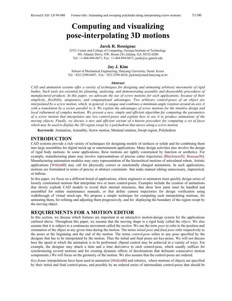
Interpolation should be independent of the design historyA rigid body motion is a continuous mapping from the time domain to a set of poses. To relieve the designers from theburden of specifying this mapping in abstract mathematical terms, combinations of simple rigid-body motion-primitives, such as linear translations or rotations around the principal axes, are often used. These simple motions areplanar and thus ill-suited, by themselves, for approximating arbitrary motions in 3D-space. Specifying combinations ofthem that should occur in parallel to produce a 3D motion is difficult and error prone, because each rotation andtranslation is expressed in a different coordinate system produced by the cumulative effect of the previous motionprimitives in the sequence. For example, Figure 1a (left) shows the superposition of several instances of a simpleobject moving along a natural motion that interpolates the initial to final control-poses. The trajectory of the object isnot surprising. The final control-pose may have been specified by the designer interactively by starting with the objectin its initial pose and applying a series of rigid body transformations (such as translations and rotations around thethree principal axes). For example, the final pose may be the result of a translation by v, followed by a rotation of anangle x around the X-axis, followed by a rotation of an angle y around the Y-axis, followed by a rotation of an angle zaround the Z-axis. A continuous motion from the initial to the final pose could be produced by animating eachtransformation, one after the other. For example, the object would first move along a straight line, then be rotatedaround the X-axis, and so on. This piecewise-simple motion would be unacceptable in many applications. The popularalternative is to animate all the transformations in the sequence simultaneously, and to combine them for each value oftime. A linear interpolation of the parameters of each transformation in this sequence would yield a parameterizedtransformation, which combines a translation by tv with rotations of angles tx, ty, and tz around the three principalaxes. As we vary t between 0 and 1, the combined transformation smoothly moves the object from its initial pose tothe final one. Unfortunately, as shown in Figure 1b (right), the resulting trajectory may be rather surprising. Theunexpected behavior shown here corresponds to a poor choice of the three angles x, y, and z, which may have resultedfrom an interactive adjustment of the final pose through trial-and-error. For example, the same final pose may havebeen obtained by replacing x by π-x and adjusting the other two angles accordingly. We advocate that the naturalinterpolation of Figure 1a should be computed automatically from the two control-poses.

Figure 1: Screw motion on the left (a) versus linear interpolation of pose parameters right (b)


Interpolations should not depend on the coordinate systemNatural motions, such as the one shown in Figure 1a , are produced by interpolations that involve a minimum anglerotation for which the direction of the axis of rotation is defined (as discussed below). However, there is a choice forselecting the location of the axis of rotation and the translation vector. Most of these choices lead to motions that areaffected by the selection of the coordinate system as discussed below, which further complicates the designer’s job[Weld90, Roschel98].

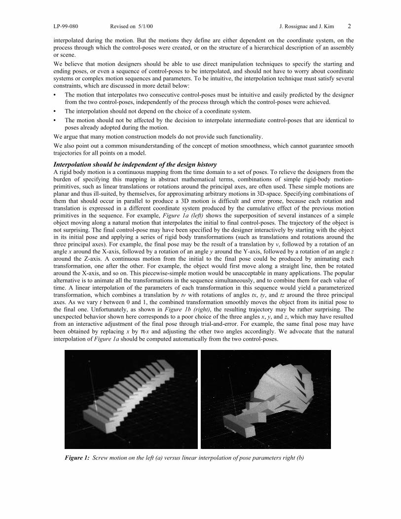
Consider the two initial and final control-poses of Figure 2A and 2B, that define the relative poses of an object (largetriangle) with respect to a camera (small triangle). For clarity, the scene (which comprises the object and the camera) isshown so that the object keeps its position and orientation throughout the illustrations of Figure 2. If the interpolatingmotion is computed as the minimum angle rotation synchronized with a straight line translation, the motion will bedifferent when it is computed in the coordinate system of the camera (Figure 2C) and when it is computed in thecoordinate system of the object (Figure 2D). The user may for example rotate an object 180 degree to obtain the finalcontrol-pose and use it to produce a motion where the object appears to rotate, or equivalently where the cameraappears to circle around the object. Depending on which coordinate system is used to compute the interpolatingmotion, a minimum angle rotation combined with a straight line translation will either produce the desired motion orwill have the camera fly right through the object.

Figure 2 Two different motions (fig. C and fig. D) defined by the same relative poses, (fig. A and fig. B), butexpressed in different coordinate systems.

To alleviate this problem, we advocate the use of interpolating screw motions, which in the 2D case degenerates into apure rotation or a pure translation, because they produce consistently the same relative trajectory (Figure 2C),regardless of the choice of coordinate systems. To pursue our example, when screw motions are used in 2D or 3D tocontrol the view, the object always appears to rotate around its center, regardless of whether the object was rotatedaround itself in the coordinate system of the camera or whether the camera was rotated around the object in worldcoordinates.

Interpolations should be stable under sub-samplingIn order to refine the motion, the designer should be able to insert a pose that is adopted during the initial motion as anew control pose. Clearly, if that insertion were to change the original motion, the designer would be surprised andwould not be able to use this subdivision approach for fine-tuning more complex motions.

To better illustrate the importance of this option and to provide a more formal notation, we describe a typical motiondesign step, as it is supported by the Meditor (motion-editor) design interface developed by the authors. The designerspecifies the initial and final control-poses, A and B, for one or a group of 3D objects. These control poses are adjustedthrough direct manipulation by dragging points on the screen with a mouse or by using a 3D input device. Theinterpolating motion is a pose-valued expression, P(t,A,B), which is parameterized by A, B, and t. The time parametert varies between 0 and 1 and the interpolation properties of the motion imply that P(0,A,B)=A and P(1,A,B)=B. Bysimply turning a dial representing the time, t, the designer changes the value of t and thus animates the object along itsmotion. If the motion is not satisfactory, the designer may adjust the two control-poses. If that is not an option,because these poses are already constrained, the designer will break the motion into two or more sub-motions. To doso, at a selected value t’ of t, the designer creates a new control-pose, M, defined as P(t’,A,B). The original singlemotion P(t,A,B) is now replaced by two motions, P(u,A,M) with u in [0, t’] and P(v,M,B) with v in [t’,1]. Theconcatenation (in time) of P(u,A,M) and P(v,M,B) produces in Meditor a motion that is identical to the original motionP(t,A,B), if we use the following mapping: for t in [0,t’], t is u; and for t in [t’,1], t is v−t’. This control-pose insertionhas replaced a single motion from A to B, denoted by A→B, by a composite motion from A to M and from M to B,

A B C D


denoted A→M→B. This change has not altered the total motion and the designer is free to adjust the result by editingM, while playing with the time knob to inspect the effect of these changes. A series of instances of the object along theresulting trajectories for discrete time samples may be used to provide feedback during this local fine-tuning.Furthermore, slight perturbations of M through translations by a relatively small vector or through rotations by a smallangle will, except at singularities, change the overall motion only slightly. In loose terms, the motion A→M→B is acontinuous function of M, and also of A and B . The property that A→P(t’,A,B)→B be identical to A→B is true forinterpolating screw-motions, but is in general not true for other interpolating motions.

The designer may also choose to insert three new key-frames somewhere in the A→B motion and produce a compositemotion A→L→M→N→B. Altering M will only affect the resulting motions between the time parameters associatedwith L and N. Thus the designer has local control over the motion.

Motion smoothness is a misleading objectiveAesthetic concerns may call for a “smooth” motion that interpolates a series of poses [Zefran98]. Although it isrelatively simple to compute interpolating motions that produce a geometrically smooth trajectory for a given point onthe object, it is more difficult to ensure trajectory smoothness for all points of the moving object simultaneously. Wesay that a trajectory is smooth when it is continuous and has a continuous tangent. Given that the interpolating motionis defined in terms of control-poses without reference to the moving object, to be smooth regardless of the object beingmoved, a motion would have to produce smooth trajectories for all points of the three-dimensional space (or at least ofa subset of that space that is guaranteed to contain the object). This is not the case for most piecewise-simple motions.Consider for instance an airplane rolling at constant speed along a 2D path made of smoothly connected circular arcs.While sliding along a single arc, the plane (and the entire space attached to it) is subject to a smooth motion (all pointsof that space travel along smooth curves). When switching between one arc and the next one, the cockpit may still besubject to a smooth motion, but the ends of the wings may abruptly change direction, and thus do not follow a smoothtrajectory. If, instead of a piecewise circular motion, we were to use a motion that is a continuous and twicedifferentiable function of the parameter t, the motion of each point would be C1, and hence smooth, although thetrajectory may not. Points on the wings of our plane would come to a halt progressively before changing directions.Although techniques exist for producing smooth interpolating motions, they do not satisfy the requirements discussedabove. Therefore, we have focused our studies on motions that are piecewise smooth. We have found, however, thatdirect manipulation of the control-poses and the local control and refinement offered by our approach enable designersto easily construct visually smooth trajectories, when required.

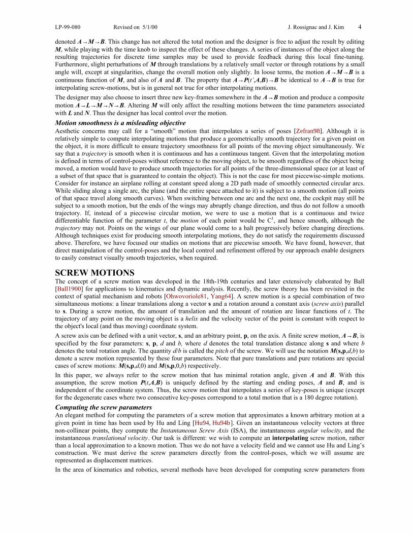
SCREW MOTIONSThe concept of a screw motion was developed in the 18th-19th centuries and later extensively elaborated by Ball[Ball1900] for applications to kinematics and dynamic analysis. Recently, the screw theory has been revisited in thecontext of spatial mechanism and robots [Ohwovoriole81, Yang64]. A screw motion is a special combination of twosimultaneous motions: a linear translations along a vector s and a rotation around a constant axis (screw axis) parallelto s. During a screw motion, the amount of translation and the amount of rotation are linear functions of t. Thetrajectory of any point on the moving object is a helix and the velocity vector of the point is constant with respect tothe object's local (and thus moving) coordinate system.

A screw axis can be defined with a unit vector, s, and an arbitrary point, p, on the axis. A finite screw motion, A→B, isspecified by the four parameters: s, p, d and b, where d denotes the total translation distance along s and where bdenotes the total rotation angle. The quantity d/b is called the pitch of the screw. We will use the notation M(s,p,d,b) todenote a screw motion represented by these four parameters. Note that pure translations and pure rotations are specialcases of screw motions: M(s,p,d,0) and M(s,p,0,b) respectively.

In this paper, we always refer to the screw motion that has minimal rotation angle, given A and B. With thisassumption, the screw motion P(t,A,B) is uniquely defined by the starting and ending poses, A and B, and isindependent of the coordinate system. Thus, the screw motion that interpolates a series of key-poses is unique (exceptfor the degenerate cases where two consecutive key-poses correspond to a total motion that is a 180 degree rotation).

Computing the screw parametersAn elegant method for computing the parameters of a screw motion that approximates a known arbitrary motion at agiven point in time has been used by Hu and Ling [Hu94, Hu94b]. Given an instantaneous velocity vectors at threenon-collinear points, they compute the Instantaneous Screw Axis (ISA), the instantaneous angular velocity, and theinstantaneous translational velocity. Our task is different: we wish to compute an interpolating screw motion, ratherthan a local approximation to a known motion. Thus we do not have a velocity field and we cannot use Hu and Ling’sconstruction. We must derive the screw parameters directly from the control-poses, which we will assume arerepresented as displacement matrices.

In the area of kinematics and robotics, several methods have been developed for computing screw parameters from


displacement matrices [Paul82, Suh78]. A variation of these methods was used in computer graphics and animation toconvert 3x3 rotation matrices to quaternions [Barr92, Pletinckx89, Shoemake85]. These methods are based on matrixinversion and thus involve a fair amount of calculations [Watt92], which are avoided by the method suggested here.

A rigid body motion transformation, T, may be represented as a 3x4 matrix, {i j k o}, formed by four column vectors,i, j, k, and o, which each have three coordinates and represent respectively the images by T of the three vectors of anorthonormal basis and of the origin. T may be used to transform an object from some nominal position and orientationinto the desired position and orientation. Therefore it defines a control-pose.

Note that when homogeneous coordinates are used, transformations may be represented as 4x4 matrices, padding theabove {i j k o} matrix with a fourth row vector (0,0,0,1). This notation introduces storage and processing redundancieswhen dealing with rigid body transformations, but is often preferred to a 3x4 notation, because it unifies therepresentations of translation, rotation, scaling, and perspective transformations. Nevertheless, we use the 3x4 notationin this paper to emphasize the meaning of the four vectors, presented above.

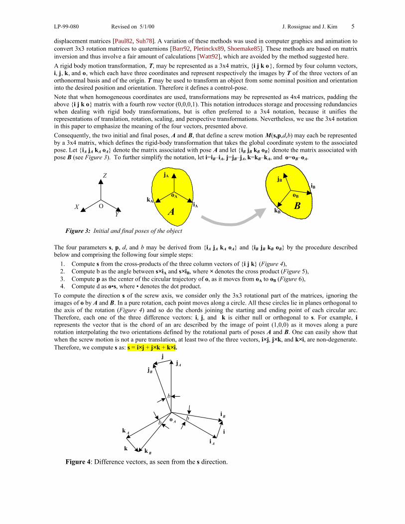
Consequently, the two initial and final poses, A and B, that define a screw motion M(s,p,d,b) may each be representedby a 3x4 matrix, which defines the rigid-body transformation that takes the global coordinate system to the associatedpose. Let {iA jA kA oA} denote the matrix associated with pose A and let {iB jB kB oB} denote the matrix associated withpose B (see Figure 3). To further simplify the notation, let i=iB–iA, j=jB–jA, k=kB–kA, and o=oB–oA.

Figure 3: Initial and final poses of the object

The four parameters s, p, d, and b may be derived from {iA jA kA oA} and {iB jB kB oB} by the procedure describedbelow and comprising the following four simple steps:

1. Compute s from the cross-products of the three column vectors of {i j k} (Figure 4),2. Compute b as the angle between s×iA and s×iB, where × denotes the cross product (Figure 5),3. Compute p as the center of the circular trajectory of o, as it moves from oA to oB (Figure 6),4. Compute d as o•s, where • denotes the dot product.

To compute the direction s of the screw axis, we consider only the 3x3 rotational part of the matrices, ignoring theimages of o by A and B. In a pure rotation, each point moves along a circle. All these circles lie in planes orthogonal tothe axis of the rotation (Figure 4) and so do the chords joining the starting and ending point of each circular arc.Therefore, each one of the three difference vectors: i, j, and k is either null or orthogonal to s. For example, irepresents the vector that is the chord of an arc described by the image of point (1,0,0) as it moves along a purerotation interpolating the two orientations defined by the rotational parts of poses A and B. One can easily show thatwhen the screw motion is not a pure translation, at least two of the three vectors, i×j, j×k, and k×i, are non-degenerate.Therefore, we compute s as: s = i×j + j×k + k×i.

Figure 4: Difference vectors, as seen from the s direction.

YX O

Z

AiA

jA

oAkA

iB

jB

oB

kBB

Ajj

Bj

Ao

Ai

Bi

iAk

Bkk

b

bb


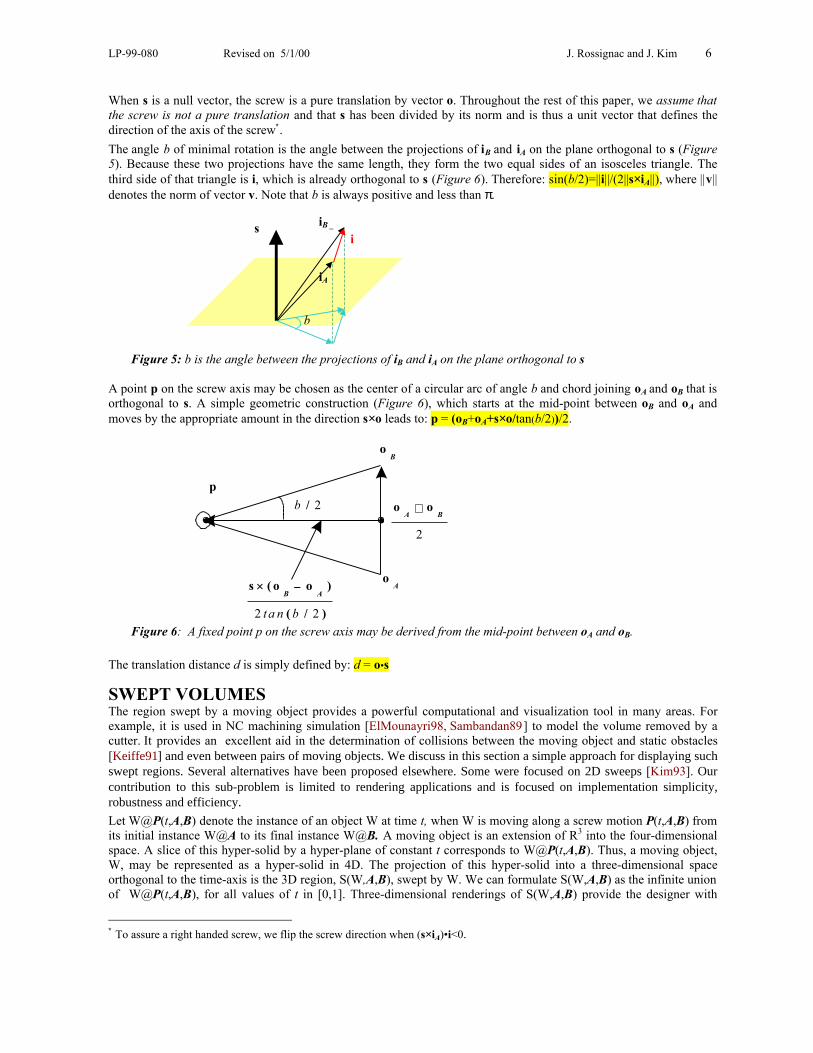
When s is a null vector, the screw is a pure translation by vector o. Throughout the rest of this paper, we assume thatthe screw is not a pure translation and that s has been divided by its norm and is thus a unit vector that defines thedirection of the axis of the screw∗.

The angle b of minimal rotation is the angle between the projections of iB and iA on the plane orthogonal to s (Figure5). Because these two projections have the same length, they form the two equal sides of an isosceles triangle. Thethird side of that triangle is i, which is already orthogonal to s (Figure 6). Therefore: sin(b/2)=||i||/(2||s×iA||), where ||v||denotes the norm of vector v. Note that b is always positive and less than π.

Figure 5: b is the angle between the projections of iB and iA on the plane orthogonal to s

A point p on the screw axis may be chosen as the center of a circular arc of angle b and chord joining oA and oB that isorthogonal to s. A simple geometric construction (Figure 6), which starts at the mid-point between oB and oA andmoves by the appropriate amount in the direction s×o leads to: p = (oB+oA+s×o/tan(b/2))/2.

Figure 6: A fixed point p on the screw axis may be derived from the mid-point between oA and oB.

The translation distance d is simply defined by: d = o•s

SWEPT VOLUMESThe region swept by a moving object provides a powerful computational and visualization tool in many areas. Forexample, it is used in NC machining simulation [ElMounayri98, Sambandan89] to model the volume removed by acutter. It provides an excellent aid in the determination of collisions between the moving object and static obstacles[Keiffe91] and even between pairs of moving objects. We discuss in this section a simple approach for displaying suchswept regions. Several alternatives have been proposed elsewhere. Some were focused on 2D sweeps [Kim93]. Ourcontribution to this sub-problem is limited to rendering applications and is focused on implementation simplicity,robustness and efficiency.

Let W@P(t,A,B) denote the instance of an object W at time t, when W is moving along a screw motion P(t,A,B) fromits initial instance W@A to its final instance W@B. A moving object is an extension of R3 into the four-dimensionalspace. A slice of this hyper-solid by a hyper-plane of constant t corresponds to W@P(t,A,B). Thus, a moving object,W, may be represented as a hyper-solid in 4D. The projection of this hyper-solid into a three-dimensional spaceorthogonal to the time-axis is the 3D region, S(W,A,B), swept by W. We can formulate S(W,A,B) as the infinite unionof W@P(t,A,B), for all values of t in [0,1]. Three-dimensional renderings of S(W,A,B) provide the designer with

∗ To assure a right handed screw, we flip the screw direction when (s×iA)•i<0.

s

iA

iiB _

b

p

2

BAoo +

Bo

Ao

)/(

)o( os

22 bta n

AB−×

2/b


powerful tools for analyzing the trajectory of the object and for studying its interaction with other objects and withpotential obstacles. We view the possibility of computing a 3D representation of S(W,A,B) that is suitable forinteractive 3D inspection as a necessary functionality in any motion design and analysis software.

For general motions, it is expensive to compute a boundary representation of S(W,A,B) [AbdelMalek98, Blackmore99,Blackmore97, Hu94, Hu94b, Parida94, Martin81, Rossignac84] and many systems resort to a graphic superposition ofthe instances of W@P(t,A,B) for a set of samples of t or to discretized models [Schroeder94]. The superposition ofmany instances of a moving object may impose a severe penalty on the rendering system. Furthermore, unless thenumber of instances is very large, the superposition produces a bumpy surface which fails to reveal the true nature ofS(W,A,B). For a piecewise-screw motion, however, the cost of computing a graphic representation of S(W,A,B) isconsiderably reduced by exploiting the following two observations.

First, instead of the boundary bS(W,A,B) of S(W,A,B), we can display the boundary of the initial instance, theboundary of the final instance, and an extrusion surface, E(W,A,B), defined below. (The b symbol is used as aboundary operator here.) Although E(W,A,B) ∪ b(W@A) ∪ b(W@B) is a superset of bS(W,A,B), the excess liesinside the swept region S(W,A,B) and thus will be hidden from the viewer, if the standard 3D graphics z-buffer test isperformed for visible surface determination. Thus, for graphics applications, and with some precautions for collisiondetection, we may use this superset and need not trim it to the exact boundary of S(W,A,B).

Second, we may define the extrusion surface, E(W,A,B), as the sweep G(W,A,B)@P(t,A,B) of a time-independentgenerator G(W,A,B). The generator is the locus of all grazing points of bW that separate the egress points that haveoutward pointing velocity from the ingress points that have inward velocity [Blackmore97]. Because, during a screwmotion, the velocity of a point is constant in the local coordinate frame of the moving object, G(W,A,B) may be pre-computed from a description of W, A, and B and then swept along the screw motion. The sweep E(W,A,B) may beeasily approximated by a series of quadrilateral or triangular graphic primitives to the desired level of accuracy.

G(W,A,B) is composed of silhouette edges (a subset of the edges of W) and of characteristic curves [Hu94] (a subsetof the faces of W). We discuss below how these are computed for polyhedral models subject to a screw motion.

Computing the characteristic curves and silhouette edgesThe sweep of the characteristic curves is the envelope of a family of surfaces Informally, the envelope of a one-parameter family of surfaces, W(t), is the limit of the intersection of W(t) and W(t+ε), as ε tends towards zero, for allvalues of t. Analytical formulation of such envelopes have been studied for a long time [Monge1849]. Envelopes ofrigid bodies under a continuous motion are a special case. Their nature depends on the type of motion and on thenature of the surfaces and edges that bound the moving object. Formulations for the envelope surfaces based on theenvelope theory [Wang86], on differential equations [Blackmore92b, Blackmore99, Ganter93], and on Jacobian RankDeficiency [AbdelMalek97, AbdelMalek98] have been explored.

Several practical techniques were introduced to compute such envelopes and to trim them to the boundaries of sweptvolumes of moving objects [Blackmore92, Blackmore99, AbdelMalek98]. Many are reviewed by Blackmore andcolleagues [Blackmore97]. Techniques restricted to polyhedral objects were studied by Weld and Leu [Weld90].Although free-from surfaces are widely used to represent geometric models in CAD, computing the envelope ofcurved surfaces is hard. A closed form solution for the restricted set of natural quadric surfaces undergoing aninstantaneous screw motion was proposed by Hu and Ling [Hu94, Hu94b]. They have further combined this techniquewith the local approximation of an arbitrary motion by an instantaneous screw motion. At each time step, theycompute an instantaneous screw motion approximation from the velocities and positions of three vertices, then theyuse the approximating screw motion to compute the characteristic curves on the faces and edges of the object in itscurrent position, and finally produce a polygonal surface that interpolates two consecutive characteristic curves, whichwe believe may have different topologies. The resulting polygonal surface is then trimmed to the part that bounds theswept volume by computing a series of cross-sections, performing a 2D selection of bounding curves, and theninterpolating the resulting 2D contour by a triangular surface. The result is a polyhedral approximation of theboundary of S(W,A,B).

We recognize that computing envelopes directly from curved objects is important for some applications. However, webelieve that it is an unnecessary expense, if the resulting sweep is to be approximated by a polyhedral model beforerendering. Since we are aiming at the computation of a polygonal approximation of the swept region, we advocate touse polygonal approximations of the moving shapes. Furthermore, since the motion is not given, but is being designed,we advocate the use of interpolating screw-motions. These two design decision simplify the software and enhance itsperformance and numeric stability.

In this section, we consider that the screw motion interpolating poses A and B is represented by its s, p, b, and dparameters, expressed in the local coordinate system of the moving object, W. This assumption may be interpreted inthree equivalent ways:

• The moving object W is already in its initial position W@A,


• s and p have been transformed by the inverse of A,

• A is the identity and B is the relative pose defined by the composition of the transformation associated with Bfollowed by the transformation associated with the inverse of A.

The velocity v(q) of a point q that is subject to a screw motion M(s,p,d,b) is the vector sum of a displacement by dalong s and a displacement by a quantity br along the vector t that is tangent to the circle which is the planar projectionalong s of the helix upon which q travels. The quantity r is the radius of that circle. Thus, we have v(q)= ds+brt.

Let pq stand for the vector q−p. The vector rt is orthogonal to both s and pq and has for magnitude the length of theprojection of pq onto a plane orthogonal to s. Consequently, rt=s×pq and we have: v(q) = ds + bs×pq.

Consider an arbitrary direction n, not parallel to s. The set of points q with velocity orthogonal to n is the surfacedefined by n•v(q)=0. Developing this equation yields n•(ds+bs×pq)=0, which becomes n•ds−bn•(s×p)+bn•(s×q)=0. Byexploiting the properties of the mixed product n•(s×q), we obtain bq•(n×s)=n•ds−bn•(s×p), which is the equation of aplane, U, with normal n×s to which the point q must belong.

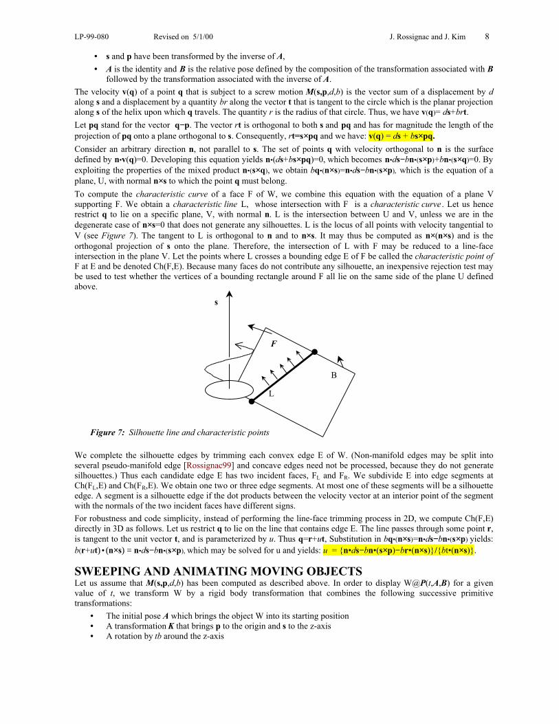
To compute the characteristic curve of a face F of W, we combine this equation with the equation of a plane Vsupporting F. We obtain a characteristic line L, whose intersection with F is a characteristic curve . Let us hencerestrict q to lie on a specific plane, V, with normal n. L is the intersection between U and V, unless we are in thedegenerate case of n×s=0 that does not generate any silhouettes. L is the locus of all points with velocity tangential toV (see Figure 7). The tangent to L is orthogonal to n and to n×s. It may thus be computed as n×(n×s) and is theorthogonal projection of s onto the plane. Therefore, the intersection of L with F may be reduced to a line-faceintersection in the plane V. Let the points where L crosses a bounding edge E of F be called the characteristic point ofF at E and be denoted Ch(F,E). Because many faces do not contribute any silhouette, an inexpensive rejection test maybe used to test whether the vertices of a bounding rectangle around F all lie on the same side of the plane U definedabove.

Figure 7: Silhouette line and characteristic points

We complete the silhouette edges by trimming each convex edge E of W. (Non-manifold edges may be split intoseveral pseudo-manifold edge [Rossignac99] and concave edges need not be processed, because they do not generatesilhouettes.) Thus each candidate edge E has two incident faces, FL and FR. We subdivide E into edge segments atCh(FL,E) and Ch(FR,E). We obtain one two or three edge segments. At most one of these segments will be a silhouetteedge. A segment is a silhouette edge if the dot products between the velocity vector at an interior point of the segmentwith the normals of the two incident faces have different signs.

For robustness and code simplicity, instead of performing the line-face trimming process in 2D, we compute Ch(F,E)directly in 3D as follows. Let us restrict q to lie on the line that contains edge E. The line passes through some point r,is tangent to the unit vector t, and is parameterized by u. Thus q=r+ut, Substitution in bq•(n×s)=n•ds−bn•(s×p) yields:b(r+ut)•(n×s) = n•ds−bn•(s×p), which may be solved for u and yields: u = {n•ds−bn•(s×p)−br•(n×s)}/{bt•(n×s)}.

SWEEPING AND ANIMATING MOVING OBJECTSLet us assume that M(s,p,d,b) has been computed as described above. In order to display W@P(t,A,B) for a givenvalue of t, we transform W by a rigid body transformation that combines the following successive primitivetransformations:

• The initial pose A which brings the object W into its starting position• A transformation K that brings p to the origin and s to the z-axis• A rotation by tb around the z-axis

F

B

L

s


• A translation by td along the z-axis• The inverse K-1 of K

A matrix representation of K-1 may be easily computed as {i j s o}, where i and j are constructed to form anorthonormal basis with s. The 3x4 matrix that represents the inverse of a rigid body transformation is easily obtainedas a composition of a 3x3 matrix that is the transpose of the rotational part of the original matrix and a translation,which is the inverse of the original translation vector transformed by the inverted rotation.

In order to produce an approximation for the face swept by each silhouette edge E joining two points a and b, wecompute the silhouette edge for W@A and compute the images a’ and b’ of its vertices by P(ε,A,B) for ε=1/k, whichdepends on the desired accuracy of the approximation [Elber97]. Then we generate the quadrilateral face bounded bythe four vertices (a, b, b’, a’). We store all these quadrilateral faces with the associated normal vectors in a displaylists, one quadrilateral per silhouette edge.

Then, we superimpose the displays of W@A, W@B, and of instances of the display list of quadrilateral edgestransformed by P(ε,A,B), P(2ε,A,B), P(3ε,A,B),…P((k-1)ε,A,B). Note that we do not need to compute thesetransformations explicitly, given that P(ε,A,B), P(2ε,A,B)°P(ε,A,B), where ° denotes the composition oftransformations.

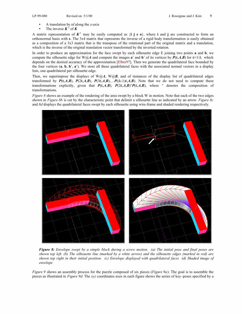
Figure 8 shows an example of the rendering of the area swept by a block W in motion. Note that each of the two edgesshown in Figure 8b is cut by the characteristic point that delimit a silhouette line as indicated by an arrow. Figure 8cand 8d displays the quadrilateral faces swept by each silhouette using wire-frame and shaded rendering respectively.

Figure 8: Envelope swept by a simple block during a screw motion. (a) The initial pose and final poses areshown top left. (b) The silhouette line (marked by a white arrow) and the silhouette edges (marked in red) areshown top right in their initial position. (c) Envelope displayed with quadrilateral faces (d) Shaded image ofenvelope

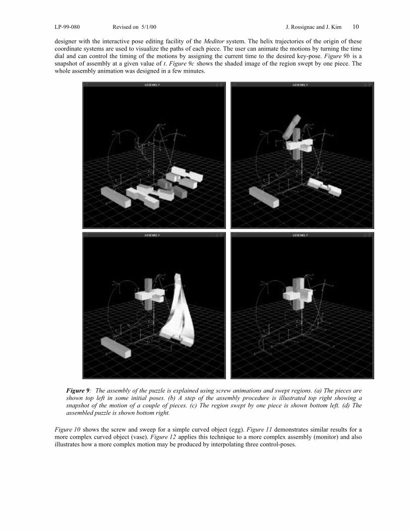
Figure 9 shows an assembly process for the puzzle composed of six pieces (Figure 9a). The goal is to assemble thepieces as illustrated in Figure 9d. The xyz coordinates axes in each figure shows the series of key–poses specified by a


designer with the interactive pose editing facility of the Meditor system. The helix trajectories of the origin of thesecoordinate systems are used to visualize the paths of each piece. The user can animate the motions by turning the timedial and can control the timing of the motions by assigning the current time to the desired key-pose. Figure 9b is asnapshot of assembly at a given value of t. Figure 9c shows the shaded image of the region swept by one piece. Thewhole assembly animation was designed in a few minutes.

Figure 9: The assembly of the puzzle is explained using screw animations and swept regions. (a) The pieces areshown top left in some initial poses. (b) A step of the assembly procedure is illustrated top right showing asnapshot of the motion of a couple of pieces. (c) The region swept by one piece is shown bottom left. (d) Theassembled puzzle is shown bottom right.

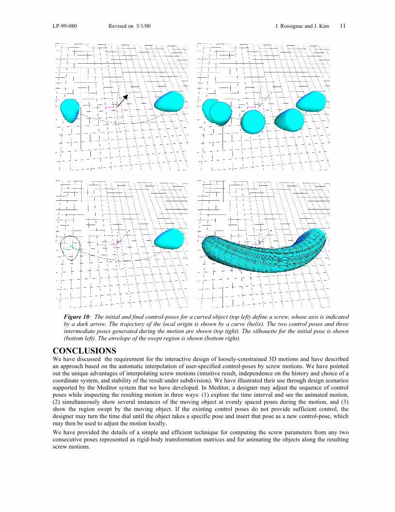
Figure 10 shows the screw and sweep for a simple curved object (egg). Figure 11 demonstrates similar results for amore complex curved object (vase). Figure 12 applies this technique to a more complex assembly (monitor) and alsoillustrates how a more complex motion may be produced by interpolating three control-poses.


Figure 10: The initial and final control-poses for a curved object (top left) define a screw, whose axis is indicatedby a dark arrow. The trajectory of the local origin is shown by a curve (helix). The two control poses and threeintermediate poses generated during the motion are shown (top tight). The silhouette for the initial pose is shown(bottom left). The envelope of the swept region is shown (bottom right).

CONCLUSIONSWe have discussed the requirement for the interactive design of loosely-constrained 3D motions and have describedan approach based on the automatic interpolation of user-specified control-poses by screw motions. We have pointedout the unique advantages of interpolating screw motions (intuitive result, independence on the history and choice of acoordinate system, and stability of the result under subdivision). We have illustrated their use through design scenariossupported by the Meditor system that we have developed. In Meditor, a designer may adjust the sequence of controlposes while inspecting the resulting motion in three ways: (1) explore the time interval and see the animated motion,(2) simultaneously show several instances of the moving object at evenly spaced poses during the motion, and (3)show the region swept by the moving object. If the existing control poses do not provide sufficient control, thedesigner may turn the time dial until the object takes a specific pose and insert that pose as a new control-pose, whichmay then be used to adjust the motion locally.

We have provided the details of a simple and efficient technique for computing the screw parameters from any twoconsecutive poses represented as rigid-body transformation matrices and for animating the objects along the resultingscrew motions.


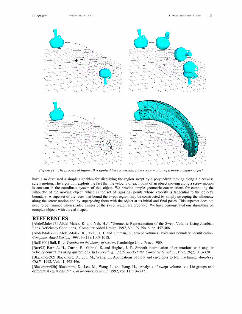
Figure 11: The process of figure 10 is applied here to visualize the screw motion of a more complex object.

have also discussed a simple algorithm for displaying the region swept by a polyhedron moving along a piecewisescrew motion. The algorithm exploits the fact that the velocity of each point of an object moving along a screw motionis constant in the coordinate system of that object. We provide simple geometric constructions for computing thesilhouette of the moving object, which is the set of (grazing) points whose velocity is tangential to the object’sboundary. A superset of the faces that bound the swept region may be constructed by simply sweeping the silhouettealong the screw motion and by superposing them with the object at its initial and final poses. This superset does notneed to be trimmed when shaded images of the swept region are produced. We have demonstrated our algorithms oncomplex objects with curved shapes.

REFERENCES[AbdelMalek97] Abdel-Malek, K. and Yeh, H.J., "Geometric Representation of the Swept Volume Using JacobianRank-Deficiency Conditions," Computer Aided Design, 1997, Vol. 29, No. 6, pp. 457-468.[AbdelMalek98] Abdel-Malek, K., Yeh, H. J. and Othman, S., Swept volumes: void and boundary identification.Computer-Aided Design, 1998, 30(13), 1009-1018.[Ball1900] Ball, R., A Treatise on the theory of screws. Cambridge Univ. Press. 1900.[Barr92] Barr, A. H., Currin, B., Gabriel, S. and Hughes, J. F., Smooth interpolation of orientations with angularvelocity constraints using quaternions. In Proceedings of SIGGRAPH ’92, Computer Graphics, 1992, 26(2), 313-320.[Blackmore92] Blackmore, D., Leu, M., Wang, L., Applications of flow and envelopes to NC machining. Annals ofCIRP, 1992, Vol. 41, 493-496.[Blackmore92b] Blackmore, D., Leu, M., Wang, L. and Jiang, H., Analysis of swept volumes via Lie groups anddifferential equations. Int, J. of Robotics Research, 1992, vol. 11, 516-537.


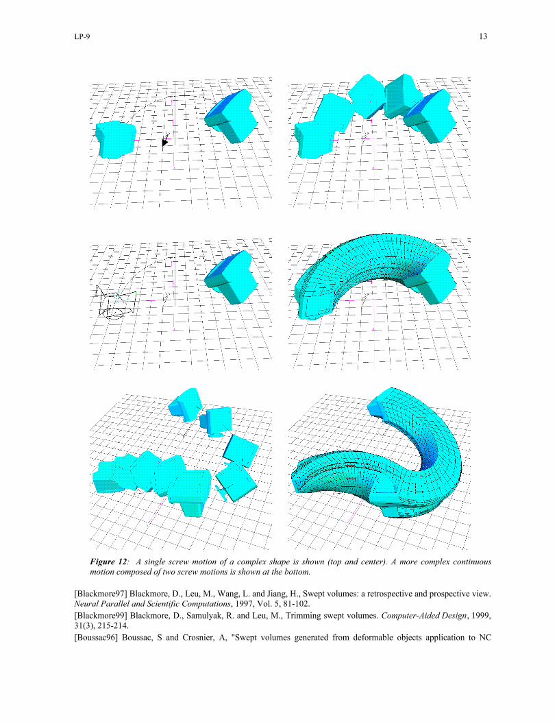
Figure 12: A single screw motion of a complex shape is shown (top and center). A more complex continuousmotion composed of two screw motions is shown at the bottom.

[Blackmore97] Blackmore, D., Leu, M., Wang, L. and Jiang, H., Swept volumes: a retrospective and prospective view.Neural Parallel and Scientific Computations, 1997, Vol. 5, 81-102.[Blackmore99] Blackmore, D., Samulyak, R. and Leu, M., Trimming swept volumes. Computer-Aided Design, 1999,31(3), 215-214.[Boussac96] Boussac, S and Crosnier, A, "Swept volumes generated from deformable objects application to NC


verification", Proceedings of the 13th IEEE International Conference on Robotics and Automation. Part 2 (of 4), 1996,Apr 22-28, vol 2, Minneapolis, MN, pp. 1813-1818.

[Bruderlin95] Bruderlin, A. and Williams, L., Motion signal processing. In Proceedings of SIGGRAPH ’95, ComputerGraphics, 1995, 293-302.[Elber97] Elber, G., "Global error bounds and amelioration of sweep surfaces'', CAD, Vol. 29, No. 6, pp. 441-449,1997.[ElMounayri98] El Mounayri, H.; Spence, A.D.; Elbestawi, M.A., 1998, Milling process simulation - a generic solidmodeller based paradigm", Journal of Manufacturing Science and Engineering, Transactions of the ASME, 1998, vol.120, no. 2, pp. 213-221.[Ganter93] Ganter, M A, Storti, D W, and Ensz, M T 'On Algebraic Methods for Implicit Swept Solids with FiniteExtent' ASME DE Vol 65(2) (1993) pp389-396.[Hu94] Hu, Z. and Ling, Z., Swept volumes generated by the natural quadric surfaces. Computers & Graphics , 1994,Vol. 20, No. 2, 263-274.[Hu94b] Hu, Z., and Ling, Z. Generating swept volumes with instantaneous screw axes”, Proc. 94 ASME DesignTechnical Conference, Part 1. Minneapolis, MN. 70(1), 7-14, 1994.[Keiffe91] Keiffe, J. and Litvin, L., Swept volume determination and interference of moving 3-D solids, ASME J. ofMechanical Design, 1991, vol. 113, 456-463.[Kim93] Kim, M.S., J.W. Ahn and S.B. Lim 1993, "Approximate General Sweep Boundary of 2D Object," CVGIP:Graphical Models and Image Processing, 1993, Vol. 55, No. 2, pp. 98-128.[Martin81] Martin, P. R. and Stephenson, P. C., Sweeping of three-dimensional objects. Computer-Aided Design,1990, 22(4), 223-234.[Monge1849] Monge, G. Applications de l’analyse a la geometrie, Paris, Bachelier, 5th edition, 1949.[Ohwovoriole81] Ohwovoriole, M. and Roth, B., An extension of screw theory. Transaction of ASME Journal ofMechanical Design, 1981, 103, 725-735.[Parida94] Parida, L and Mudur, S P 'Computational Methods for Evaluating Swept Object Boundaries' VisualComputer Vol. 10(5) (1994) pp. 266-276.[Paul82] Paul, R., Robot manipulators, MIT Press. 1982.[Pletinckx89] Pletinckx, D., Quaternion calculus as a basic tools in computer graphics. The Visual Computer, 1989,Vol. 5, 2-13.[Roschel98] Roschel, O., Rational motion design-a survey. Computer-Aided Design, 1998, 30(3), 169-178.[Rossignac84] Rossignac, J. and Requicha, A. A. G., Constant radius blending in solid modeling. Computers inMechanical Engineering, July 1984, 65-73.[Rossignac99] Rossignac, J. and Cardoze, Matchmaker: Manifold BReps for non-manifold r-sets. Proceedings of theACM Symposium on Solid Modeling, pp. 31-41, 1999.[Sambandan89] Sambandan, K and Wang, K K 'Five-axis Swept Volumes for Graphic NC Simulation andVerification' ASME DE, vol. 19(1) (1989) pp143-150.[Shoemake85] Shoemake, K., Animating rotation with quaternion curves. In Proceedings of SIGGRAPH ’85,Computer Graphics, 1985, 19(3), 245-254.[Schroeder94] Schroeder, W J, Lorensen, W E, and Linthicum, S 'Implicit Modeling of Swept Surfaces and Volumes'Proceedings of the IEEE Visualization Conference, Los Alamitos, CA (1994) pp40-45.[Suh78] Suh, C. and Radcliffe, C., Kinematics & mechanisms design. John Wiley & Sons. 1978.[Wang86] Wang, W.P. and Wang, K. K., Geometric Modeling for Swept Volume of Moving Solids, IEEE ComputerGraphics and Applications, 1986, 6(12), 8-17.[Watt92] Watt, A. and Watt, M., Advanced animation and rendering techniques, Addison-Wesley, ACM Press.1992.[Weld90] Weld J., and Leu M., Geometric representation of swept volumes with applications to polyhedral object. Int.J. Robotics Res, 1990; 9, 105-106.[Witkin88] Witkin, A. and Kass, M., Spacetime Constraints., In Proceedings of SIGGRAPH ’88, Computer Graphics ,1988, 22(4), 159-168.[Yang64] Yang, A. and Freudenstein, F., Application of dual-number quaternion algebra to the analysis of spatialmechanisms. Transaction of ASME Journal of Mechanical Design, 1964.[Zefran98] Zefran, M. and Kumar V., Interpolation schemes for rigid body motions. Computer-Aided Design , 1998,30(3), 179-189.

Computing and visualizing pose-interpolating 3D motions

Documents