COMPUTATIONAL FLUID DYNAMIC (CFD) SIMULATION OF SLUG …

COMPUTATIONAL FLUID DYNAMIC (CFD)

SIMULATION OF SLUG FLOW WITHIN PIPE BEND AND

PIPE ELBOW WHICH INDUCE VIBRATION

MOHAMED IKRAM BIN MOHAMED KHAIRI

MECHANICAL ENGINEERING

UNIVERSITI TEKNOLOGI PETRONAS

JANUARY 2020

MO

HA

ME

D IK

RA

M B

IN M

OH

AM

ED

KH

AIR

I JA

NU

AR

Y 2

02

0

B. E

NG

. (HO

NS

) ME

CH

AN

ICA

L E

NG

INE

ER

ING

i

CERTIFICATION OF APPROVAL

“Computational Fluid Dynamic (CFD) Simulation of Slug Flow

Within Pipe Bend and Pipe Elbow Which Induce Vibration

by

MOHAMED IKRAM BIN MOHAMED KHAIRI

22731

“A project dissertation submitted to the”

“Mechanical Engineering Programme”

“Universiti Teknologi PETRONAS”

“in partial fulfilment of the requirement for the”

BACHELOR OF ENGINEERING (Hons)

(MECHANICAL ENGINEERING)

Approved by,

_____________________

(Dr. William Pao)

UNIVERSITI TEKNOLOGI PETRONAS

TRONOH, PERAK

JANUARY 2020

ii

CERTIFICATION OF ORIGINALITY

“This is to certify that I am responsible for the work submitted in this project, that the

original work is my own except as specified in the references and acknowledgements,

and that the original work contained herein have not been undertaken or done by

unspecified sources or persons.”

___________________________________________

(MOHAMED IKRAM BIN MOHAMED KHAIRI)

iii

ABSTRACT

Multi-phase flow is any fluid stream consisting of more than one phase

or component, for example, gas-liquid stream, liquid-liquid flow, solid fluid

stream, or solid-fluid gas stream. It is common in fluid systems, in particular in

oil and gas hydrocarbon conveying systems which produce natural gas and

crude oil at the same time. A significant response from flux-induced vibration

can lead to potential fatigue damage or uncontrolled vibration when the

frequency of excitation matches the piping system's natural frequencies,

especially in cases where oil produces dense sand particles or slow flows in the

flow-lines. This is why it is important to investigate the impact of the oil-gas-

water mix on pipeline structure. Due to its difficulty and unpredictability,

multi-phase flow problems remain a concern for industry. The present paper

analyses the interaction between the fluid-structure fluid and a pipe bend to

determine the resultant vibrations generated by the two-phase fluid flux. For

research there are two pipe bend models with different bending upstream and

downstream lengths. Natural frequencies are eliminated and numerical

simulations are performed by the ANSYS Workbench using the CFD solver

(ANSYS FLUENT). The frequency of vibrations are obtained and compared

with naturally occurring frequencies to assess the correct degree of risk through

the transformation of the time domain results into frequency domain.

iv

ACKNOWLEGEMENT

My completion of Final Year Project I would not be a triumph without

the assistance and direction from my supervisor and colleagues. So, I would

like to recognize my heartfelt gratitude to those I honour in realizing the

progress of Final Year Project I.

First of all, I would like to extend my sincere thanks to Dr William Pao King

Soon, my direct supervisor, for his valuable supervision, encouragement,

assistance and assistance during my project. In particular on the technical

aspects, I would like to thank him for his work at Universiti Teknologi

PETRONAS.

I would also like to thank Dr. Shakif Nasif which had greatly assisted

me in learning the ANSYS Software from the beginning. I additionally wish to

offer my thanks to my kind colleagues, who were consistently there to give

significant recommendations and remarks on my works for further

improvement.

Last but not least, I wish to thank my parents and the members of my

family for their support. I managed to perform well and persevered through any

challenges faced during the project, with their help.

v

TABLE OF CONTENTS

CERTIFICATION OF APPROVAL i

CERTIFICATION OF ORIGINALITY ii

ABSTRACT iii

ACKNOWLEGEMENT iv

LIST OF FIGURES vii

LIST OF TABLES viii

CHAPTER 1: INTRODUCTION 1

1.1 Project Background 1

1.2 Problem Statement 2

1.3 Objectives 3

1.4 Scope of Study 3

CHAPTER 2: LITERATURE REVIEW 4

2.1 Multiphase Flow 4

2.2 Pipe Bend 8

2.3 Flow Pattern of Two Phases Flow 12

CHAPTER 3: METHODOLOGY 17

3.1 Description of the Problem 17

3.2 Multiphase Flow Modeling 19

3.3 Development of Fluid Domain Model 22

3.4 Meshing of Pipe and Fluid Domain 24

3.5 Modal Analysis 25

3.6 Screening Methodology 25

3.7 Project Process Flow Chart 27

vi

3.8 Project Gantt Chart 28

CHAPTER 4: RESULTS AND DISCUSSION 29

4.1 Validation of flow pattern on Baker’s map 29

4.2 The transition of slug flow pattern in a horizontal pipe 30

4.3 Validation of model against Experimental figures 32

4.4 Parametric analysis on diameter ratio of the orifice plate 35

CHAPTER 5: CONCLUSIONS AND RECOMMENDATIONS 46

REFERENCES 48

vii

LIST OF FIGURES

Figure 1.2.1: Dislodging of supporting mechanisms in pipeline [3]. ..........................2

Figure 2.1.1: Flow Regimes in Horizontal Pipes (Source:

https://build.openmodelica.org) .................................................................................5

Figure 2.1.2 : Flow Pattern Map of Crude Oil and Natural Gas at 68 atm ..................6

Figure 2.1.3: Gas-Liquid flow Regime Map for Horizontal Pipe. (Adapted from

Shell DEP 31.22.05.11):............................................................................................7

Figure 2.2.1: Summary of the studies in two phase flow and multiphase flow in

different types of pipe bend .......................................................................................8

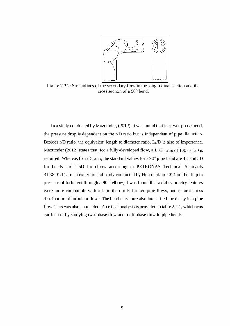
Figure 2.2.2: Streamlines of the secondary flow in the longitudinal section and the

cross section of a 90° bend. .......................................................................................9

Figure 2.3.1: Region of flow components in pipe [6]. .............................................. 13

Figure 2.3.2: Baker Chart [6]. ................................................................................. 16

Figure 3.1.1: Horizontal bending pipe geometry of the computational modelling. ... 18

Figure 3.4.1: Mesh Of (A) Pipe Bend (B) Fluid Domain ......................................... 24

Figure 3.6.1: Locations monitored (At bend) ........................................................... 25

Figure 3.7.1: Project Flow Chart ............................................................................. 27

Figure 4.1.1: Contour of water volume fraction on slug development. (a) De

Schepper et al. (2008) model, (b) Present model, (c) Mohmmed (2016) model. ....... 29

Figure 4.2.1: Water volume fraction contours of slug flow in the pipe. .................... 31

Figure 4.2.2: Time evolution contours of Slug flow and the water volume fraction

air-water towards the pipe’s elbow for (Usa = 3.07 m/s and Usw = 0.4 m/s). ............. 32

Figure 4.3.1: The schematic diagram of the experimental apparatus [16]. ................ 33

Figure 4.3.2: The evaluation of slug progression between experimental work and

CFD data simulation on water volume fraction for Usa = 1.88 m/s, Usw = 0.77 m/s (a)

Stratified pattern, (b) Crest jump and (c) slug pattern. ............................................. 34

Figure 4.3.3: Contour of Slug flow water volume fraction, snapshot of experimental

works and simulation for Usa = 1.88 m/s, Usw = 0.77 m/s. ........................................ 35

Figure 4.4.1: Time record of water volume fraction on the cross sectional pipe

located before elbow when increases air superficial velocity from 3.08 m/s to 6.45

m/s with constant water superficial velocity, Usw = 0.4 m/s. ................................... 37

Figure 4.4.2: The total exerted pressure on elbow’s wall against air inlet superficial

velocity with r/D ratio from 1.0 to 3.0 for graph (a) (b) (c) (d) with constant inlet Usw

viii

= 0.4 m/s. ................................................................................................................ 40

Figure 4.4.3: The total exerted pressure on elbow’s wall against r/D ratio with air

inlet superficial velocity from 3.07 m/s to 6.45 m/s for graph (a) (b) (c) (d) with

constant inlet Usw = 0.4 m/s. .................................................................................... 42

Figure 4.4.4: The resultant force on elbow’s wall against r/D ratio with air inlet

superficial velocity from 3.08 m/s to 6.45 m/s for graph (a) (b) (c) (d) with constant

inlet Usw = 0.4 m/s................................................................................................... 45

LIST OF TABLES

Table 2.1.1: Table Comparison of Single Phase and Multiphase ................................4

Table 2.1.2: Flow regimes of a Two-Phase Gas-Liquid Flow ....................................5

Table 2.2.1: Critical Analysis .................................................................................. 10

Table 3.1.1: Properties of Materials used in simulation ........................................... 18

Table 3.3.1: Pipeline parameters. ............................................................................ 23

Table 3.3.2:Boundary Conditions ............................................................................ 23

Table 3.4.1: Difference in Mesh properties of FEA and CFD .................................. 24

Table 3.6.1: Properties measured at locations of interest.......................................... 26

Table 3.8.1: Project Gantt Chart .............................................................................. 28

Table 4.1.1: Simulation of the air-water operating condition for slug development. . 29

Table 4.4.1: The inlet boundary condition for parametric study. .............................. 36

Table 4.4.2: Approximate time for Slug to arrive at pipe’s elbow. ........................... 37

Table 4.4.3: Water volume fraction contour on slug development for each condition

of air inlet superficial velocity ................................................................................. 38

Table 4.4.4: Pressure Contour at Measurement Section 1 and 2 with varies value of

r/D ratio and air superficial velocity at constant inlet Usw = 0.4 m/s.......................... 43

1

INTRODUCTION

Project Background

For the exchange of fluids between two or more remote stations, pipelines

are used. In oil and gas processing and distribution plants, gas and liquid two-

phase flows in pipelines occurred. Due to the constant supplied energy needs, the

transmission pipelines are the main arteries for the petroleum and gas industry.

The simultaneous 2 or more phases through a pipe is called multi-phase

flow. The two-phase mix may be carbon / gas (oil & water) and non-solid (carbon

& slot) and gas-liquid or gas-pulverized fuel. This can be gas resistant.

(pulverized coal) Gas-fluid flow is the most common two-phase flow and can be

used in a wide variety of industrial applications in the oil and gas industries,

including the chemical industry. In certain cases, a multiphase flow for the oil and

natural gas reserves include the upstream piping network and extracting

hydrocarbons, such as the spreading of the split pipe, exporting medium and the

extraction of oil pumps. For several decades two-stage gas-liquid flows,

particularly in the oil and natural gas fields, have been the subject of research

interest, operating in several pipelines under various flow conditions.

The pipe flow would have different flow rates depending on the surface gas

and fluid velocities respectively. This flow regime will vary from the gentle,

smooth layered flow to the rough, scattered ring flow. The slug flow behavior in

the pipelines can be attributed to different Fluid properties, including viscosities

and densities but particularly surface speeds in both phases. The flow mechanism

also puts great importance on the fluid layout of the ducts, including pipe length,

diameter, orientation and tilting towards or toward gravity.

2

Problem Statement

FSI is one of the important keys to flow assurance issues because excessive

vibrations arising from FSI can cause dislodging of pipelines from the supporting

mechanisms such as hangers and thrust blocks as well as an increased risk for pipe

breakage. Whereas, perturbations in velocity and pressure of the flow could cause

unsmooth flow and pose great problems to flow assurance as shown in Figure 1.2.1.

This problem is magnified in a multiphase flow, especially in a slug flow. To predict

the resulting effects of multiphase flow FSI, the first thing needed is to model and

predict the detailed behaviour of the multiphase flow as well as the patterns that they

exhibit. Then, the piping structure comes into play. In this project, it is within a pipe

bend. Turning elements such as T-junctions and bends are the locations that are most

subjected to flow-induced forces due to the changes of momentum of the fluids. The

effects of fluid flow on the adjacent structure or body, i.e. piping structure, vary with

the fluid flow characteristics, including its compositions, density, viscosity, volatility

and turbulence.

Figure 1.2.1: Dislodging of supporting mechanisms in pipeline [3].

Multiphase flow often presents a far more complex and unpredictable flow

behaviour than single phase flow. Consequently, the FSI arising from multiphase flow

is difficult to predict. One of the reasons is because the density and other properties of

the fluid are very difficult to estimate as different phase and components exist.

Simulation often requires very high computing power, not to mention multiphase flow

FSI simulation where the model can be very complex. Fortunately, computational

methods have evolved over the past decades witnessing the birth of high-performance

3

computers and powerful computing software such as ANSYS. These breakthroughs

have given new breath to FSI modelling and prediction.

However so, even in simplified simulation where only two-phase - crude oil

(liquid) and gas phase, the density, compositions, and other properties of the fluid vary

from each reservoir depending on its nature, temperature and pressure, age of reservoir

and composition. Thus, there are many variables that have to be taken into

consideration and there are variables that have to be assumed during multiphase flow

FSI simulation.

Objectives

For this project, numerical simulation of liquid-liquid flow is conducted and aimed:

a) To determine the effect of bending radius on pressure exerted on the wall

of elbow that results in flow-induced vibration arising from multiphase

flow within a horizontal pipe bend by using Computational Fluid Dynamic

(CFD).

b) To correlate r/D ratio of pipe’s elbow with 90° of bending angle.

Scope of Study

The study's main focus is to construct a two-phase flow simulation in a horizontal

pipe with various geometric parameters using ANSYS FLUENT. The Fluid Volume

(VOF) model was used to model the slug flow pattern hydrodynamics. The chosen

pipe type was circular cross-sectional shapes with an internal diameter of 0.08 m and

12 m long. Isothermal conditions are likely to extend to the internal pipe wall. Air and

water served as fluids for operations. The measurement of geometric parameters was

bending radius over diameter (r / D) ratio while the operating parameter was inlet air

and superficial velocity of the water.

4

LITERATURE REVIEW

Multiphase Flow

De Schepper et al. (2008) characterizes multiphase flow as a concurrent flow of

materials with particular states or stages, for example, gas, fluid or solid. It can

likewise be a flow of materials in a similar state or phase however with various

compound properties, for example, oil-droplets in water. According to Bakker (2005)

also, there are several regimes of multiphase flow. An example distinguishing single

phase and multiphase is shown in Table 2.1.1. In the context of this thesis, the main

concern is on two-phase gas-liquid flow.

Multiphase flow modelling is a very complex work. Not only there are limitations

in time, computing power is also a key to whether or not a multiphase flow can be

modelled accurately. Some models have been developed that are suitable for different

multiphase flow applications and exhibit different levels of accuracy and applications;

they are Eulerian-Lagrangian, Eulerian-Eulerian, Volume of Fluid, etc.

Table 2.1.1: Table Comparison of Single Phase and Multiphase

Single component Multi-component

Single Phase Water

Pure Nitrogen

Air

H2O + Oil Emulsions

Multiphase

Steam bubble in H2O

Ice Slurry

Coal Particles in Air

Sand Particles in H2O

Similar to single-phase flow, a multiphase flow follows the three main

conservation principles, namely the conservation of mass, momentum and energy.

These principles apply for each phase in a multiphase flow. Therefore, there would be

5

at least two sets of each of the conservation laws in multiphase flow. Simplifications

were made by some pioneers such as Kim and Chang (2008) for multiphase flow.

There are several two-phase gas-liquid flow regimes. They are shown in Figure 2.1.1,

and are summarized in Table 2.1.2. A flow regime explains how the phases are

distributed geometrically. Even influencing phase distribution, velocity distribution

and so on is the system in which the fluid flows (Chica, 2012).

Figure 2.1.1: Flow Regimes in Horizontal Pipes (Source:

https://build.openmodelica.org)

Table 2.1.2: Flow regimes of a Two-Phase Gas-Liquid Flow

Multiphase Flow Regime Characteristics

Bubbly flow (a) Discrete gaseous bubbles in a continuous liquid.

Stratified and free-surface

flow (b)

Immiscible fluids isolated by a characterized

interface.

Wavy flow (c) Superficial velocity of gas increases and waves

starts forming at the interface boundary due to

surface tension.

6

Slug flow (d) Discontinuous elongated bubbles separated by

chunks of liquids that blocks the pipe.

Annular flow (e) Continuous liquid around walls, core gas. It occurs

because of the high superficial gas velocity as

opposed to the air.

As to simulate the flow in the desired flow pattern, a flow regime map is to be

referred, such as the Taitel-Dukler flow regime map as shown in Figure 2.1.2. The

Taitel-Dukler flow regime map is based on the superficial velocities of the phases.

Another flow-regime map as adapted by Shell Design and Engineering Practice (DEP)

Standard 31.22.05.11 is the gas-liquid two-phase flow regime map (Figure 2.1.3) based

on the Froude numbers of each phase.

Figure 2.1.2 : Flow Pattern Map of Crude Oil and Natural Gas at 68 atm

7

Figure 2.1.3: Gas-Liquid flow Regime Map for Horizontal Pipe. (Adapted from

Shell DEP 31.22.05.11):

Chica (2012) developed a screening methodology for assessing flow-induced

vibration (FIV) due to multiphase flows using a combination of STAR-CCM+ tool and

FEA code ABAQUS. Comparisons were made between two-phase and three-phase

flows. Kadri et al. (2012) researched on the suitable parameterization to simulate slug

flows using Volume-of-Fluid method. Suitable parameterization is important for

accuracy and computation speed. Less compressive schemes are preferred instead of

the most compressive scheme because it allows for coarser meshes while maintaining

fine accuracy and avoiding numerical errors. Riverin et al. (2006) discussed that the

source of FSI excitation can be due to swift changes in flow and pressure or due to

mechanical action of the piping. Riverin et al. (2007) successfully simulated two-phase

slug flow using ANSYS CFX and validated his results with experiment. The results

shown that CFX calculation were very accurate in predicting flow pattern formed by

two-phase flow.

De Schepper et al. (2008) argues that unlike single-phase flow where an entrance

length of 30 to 50 diameters is required for fully developed turbulent flow, multiphase

flow is complex and the corresponding entrance lengths are less well established. He

emphasizes that a flow regime map does not always accurately predict a certain flow

pattern for a given fluids with given flow rates.

8

Pipe Bend

The design of pipeline systems needs to go through a series of phases, according

to Miwa (2015), which are: initial design, feasibility tests, practical design,

optimization and risk assessment. Fast changes in the flow rates and direction of liquid

or two-phase piping systems may cause transient pressure producing bursts of pressure

and transient forces inside the piping system. Regularly difficult to measure and

calculate are the magnitudes of these pressure bursts and force transients. In designing

pipe bends, there are a certain standard that have to be followed, especially for the

multi- billion-dollar oil and gas application. Figure 2.2.1 shows the summary of the

studies in two phase flow and multiphase flow in different types of pipe bend.

Figure 2.2.1: Summary of the studies in two phase flow and multiphase flow in

different types of pipe bend

According to Mazumder (2012) the curvature of the tubular bend

produces a centrifugal force which is guided from the momentary core to

the outer wall. The combination of the wall boundary layer causes indirect

flow by fluid adhesion to the wall and the centrifugal force, as seen in

Figure 2.2.2. This secondary stream is optimally compensated by the tube

axis. As a consequence, the helical shape becomes simplified by the

bending.

9

Figure 2.2.2: Streamlines of the secondary flow in the longitudinal section and the

cross section of a 90° bend.

In a study conducted by Mazumder, (2012), it was found that in a two- phase bend,

the pressure drop is dependent on the r/D ratio but is independent of pipe diameters.

Besides r/D ratio, the equivalent length to diameter ratio, Le/D is also of importance.

Mazumder (2012) states that, for a fully-developed flow, a Le/D ratio of 100 to 150 is

required. Whereas for r/D ratio, the standard values for a 90° pipe bend are 4D and 5D

for bends and 1.5D for elbow according to PETRONAS Technical Standards

31.38.01.11. In an experimental study conducted by Hou et al. in 2014 on the drop in

pressure of turbulent through a 90 ° elbow, it was found that axial symmetry features

were more compatible with a fluid than fully formed pipe flows, and natural stress

distribution of turbulent flows. The bend curvature also intensified the decay in a pipe

flow. This was also concluded. A critical analysis is provided in table 2.2.1, which was

carried out by studying two-phase flow and multiphase flow in pipe bends.

10

Table 2.2.1: Critical Analysis

Author / Date Phase Geometrical

Parameter /

Operating Conditions

Remark Result

Yadav, Worosz, Kim, Tien

& Bajorek (2014) [5]

Two-phase

flow.

90° vertical-upward

elbow.

(L/D=3, L/D=9,

L/D=21, L/D=33).

1. Experiments were

carried out on 90°

vertical-upward air–

water flows.

2. The investigation

focuses on the effect

of the elbow’s length

and diameter (L/D)

ratio on the dissipation

of bubbles across the

pipeline system.

1. In single-phase flow conditions the

elbow-effects are closely

associated with the elbow-effects.

2. The elbow effects on the two-phase

flow parameters (vibration-

inducing bubbles) vanish with an

enhanced L / D ratio for the elbow.

Mazumder (2012) [8] Multiphase 90° vertical to

horizontal elbows.

(1.5<r/D>3)

1. Experiments were

carried out on 90°

vertical to horizontal

elbows.

2. This investigation

focuses on the effect

of elbow’s bending

radius and diameter

ratios toward the radial

velocity and pressure

in the elbow.

1. Variations of r/D ratio resulting in

different flow velocities and

pressure as increasing r/D ratio

effect in the decreasing of flow

velocity and pressure in the elbow.

2. The pressure across the elbow

decreases when the bending radius

of the elbow increased.

11

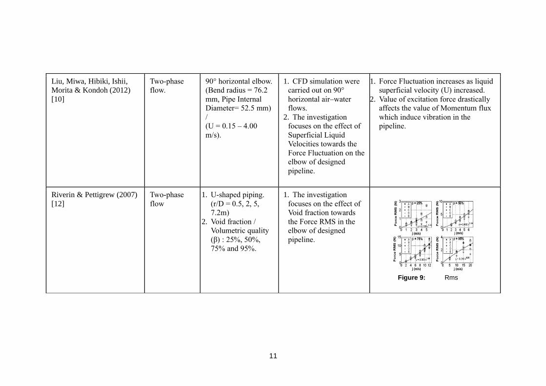
Liu, Miwa, Hibiki, Ishii,

Morita & Kondoh (2012)

[10]

Two-phase

flow.

90° horizontal elbow.

(Bend radius = 76.2

mm, Pipe Internal

Diameter= 52.5 mm)

/

(U = 0.15 – 4.00

m/s).

1. CFD simulation were

carried out on 90°

horizontal air–water

flows.

2. The investigation

focuses on the effect of

Superficial Liquid

Velocities towards the

Force Fluctuation on the

elbow of designed

pipeline.

1. Force Fluctuation increases as liquid

superficial velocity (U) increased.

2. Value of excitation force drastically

affects the value of Momentum flux

which induce vibration in the

pipeline.

Riverin & Pettigrew (2007)

[12]

Two-phase

flow

1. U-shaped piping.

(r/D = 0.5, 2, 5,

7.2m)

2. Void fraction /

Volumetric quality

(β) : 25%, 50%,

75% and 95%.

1. The investigation

focuses on the effect of

Void fraction towards

the Force RMS in the

elbow of designed

pipeline.

Figure 9: Rms value of forces versus

12

Flow Pattern of Two Phases Flow

2.3.1 Horizontal Flow Schemes in Pipe

The two-phase flux patterns in horizontal pipes are close to vertical flow, but

the liquid distribution is determined by gravity. When gravity perpendicular to the

piper axes, the liquid is compressed to the bottom of the tube and to the surface. De

Schepper et al. (2008) set out various horizontal pipe flux patterns in gas or liquid flow

which are roughly the following categories.:

Stratified flow: Two phases are completely segregated at low superficial velocities of

liquid and gas. The gas flow is isolated by smooth horizontal interface on top of the

oil. However, an increase in gas speed leads to the development of waves on the

interface which produce wavy layers.

Intermittent flow: For further changes in gas level, interfacial wave rises and a fluid

system is known as intermittent flow. This form of flow is a slug and connecting

combination. The following are listed in these subcategories:

Plug flow: Liquid connections are isolated into this flow network by elongated gas

bubbles. On the layer of big waves are the huge bubbles that float along the top of the

vessel. Plug flow is often referred to as extended bubble flow.

Slug flow: Fluid bubbling aeration happens at high gas levels, producing tiny gas

bubbles. The gas bubbles rise and the bubbles stop. The waves of great amplitude can

also be seen in the liquid slugs that distinguish these long bubbles. Such waves touch

the top of the pipe and produce a flowing slug that flows quickly through the pipe. The

two key causes of pipeline fatigue in the flow structure are plug and slug flow.

Bubbly flow: The gas bubbles in the upper part of the pipe are completely scattered

with a large number of bulbs due to the thriving powers. The turbulence intensity is

enough to evenly distribute the bubbles through the pipe at a high fluid level, or if the

cuts dominate. The upper component of the pipe pool in bubbles tends to be tidal.

Annular flow: As the speed of the gas increases, the liquid forms a ring-film around

the tube, which is thicker on the bottom than on the top due to the gravity.

13

2.3.2 Superficial Velocity

In single-phase flow, instantaneous average velocity was also described as

volumetric Q [m3/s] divided between cross-sectional pipe area A [m2].

The concept of average speed in multi-phase flow is becoming a difficult issue.

The region of a certain process, as shown in Figure 2.3.1, varies in time and space and

thus the flow no further equals the speed. A network of flows is defined by a superficial

speed. Using superficial speed has the advantage of being maintained irrespective of

the complexity of the flow mechanism (for incompressible flux without any change of

phase), e.g. The superficial speed remains constant even though the speed at the local

level is different when the flow rate is moved from the bubble to the slow flow. Maps

with the surface gas speed on one axis and the superficial fluid speed on the other are

called nutrient diagrams and are used to describe the limits of the various regimes.

ANSYS CFD-Post allows users automatically to show superficial rapid velocity or

(true) speed variables while viewing the effects of multi-phase simulations.

Sometimes the use of a superficial speed is frequently seen in correlations of

pressure drop for porous areas, whether the real porosity or the pore represents flow

obstructions. An experimentalist can define his device with superficial or real pace,

but it is useful to understand that using superficial velocity is more common when

testing data, since this can be measured outside the porous region.

Figure 2.3.1: Region of flow components in pipe [6].

True (phase) velocities are defined as:

LL

L

QU

A= (2.1)

GG

G

QU

A= (2.2)

14

UL is superficial velocity of liquid, UG is superficial velocity of gas, AL is the symbole

of area of liquid in the pipe while AG is the area of gas concentration in the pipe, QL is

liquid volumetric flow rate, QG is gas volumetric flow rate.

The superficial gas and liquid velocities and mixture velocity are defined by:

LSL L L

QU U

A= = (2.3)

GSG G G

QU U

A= = (2.4)

GG

A

A = (2.5)

LL

A

A = (2.6)

1G L + = (2.7)

M SL SGU U U= + (2.8)

Where USL is a superficial liquid speed, USG is a superficial gas speed, αG (measured

fraction) and αL (liquid holdup), respectively, the volume fraction of gas and liquid,

A is a sectional region, and UM has a mixed speed.

The total speed is proportionate to that of the volumetric flow that can be

observed, as the average instantaneous velocity of the loop would have been by taking

the entire cross-section of the pipe. Since it takes just half, surface speed tends to be

less than the real average speed.

2.3.3 Categories of Flow Regime Map in Pipe

The flow pattern map of Baker (1954) is one of the oldest and perhaps most

frequently employed, particularly in the petroleum sector. Based on industry-relevant

data, the map was created by visually evaluating the different flow regimes. They

researched transformational terms between the five flow regimes of stratified,

15

stratified, sluggish, ring, and bubbly flow, beginning at each stage of laminated flow

with a one-dimensional energy balance. He addressed this issue with the visualization

of a layered fluid and then understood how to anticipate the change from the layered

flux and how this process can be accomplished. The layered flow doesn't have to

happen because the way they form in a certain flow pattern is established in a certain

gas and liquid flow rate. Slow flows may also be referred to as this method. Taitel and

Dukler created a mechanical flow model diagram, which can predict a two-phase flow

pattern under various system conditions.

2.3.3.1 Two Phase Baker Map

For many industrial applications, the two-stage gas-liquid flows

through the horizontal pipeline. The key prevision in the field of multiphased

flow insurance is a two-phase gas-liquid flow supply in the pipeline. Typically,

defined flow pattern maps are used to define flow pattern type, without

complete calculation. The map is created by classifying different flow schemes

on the basis of data from industry. In the measurements of flow-parameters on

pipes (pressure-dependent, void-factor, heat and mass transfer etc.) Baker

(1954) [6] first commented on the importance of flow patterns. During his

work, he introduced in a circular pipe, as seen in Figure 2.3.2, the first flow

design plan for the horizontal flow. He has also identified fluid patterns in plug

stream, wave flow, bubble flow, ring flow, stratified flow and close flows. His

experimental data are well matched with the widespread flow diagram.

GL/GG are shown in figure 2.3.2, which varies from the flow pattern

characteristics that suit Baker's chart according to its boundaries by the role of

the mass flows of gas, GG and liquid and gas mass flow ratio.

Parameters for the map to be represented in any gas / liquid mixture

other than the normal flow mix are λ and ψ dimensional parameters. In the

rising mixture at atmosphere and room temperatures of 25 ° C air and water

would possibly equivalently have the λ and ψ parameters. The correct value of

λ and ψ is determined by modeling the two-stakes dynamics of any gaseous

(GG) and liquid (GL) at various temperature and pressure levels using the same

16

diagram. Although solid lines illustrate transition flow systems for region-to-

area as shown in Figure 2.3.2, they actually represent large transition regions.

Figure 2.3.2: Baker Chart [6].

For use of the map, fluid and gas flux (air, vapor) must be assessed first. The λ

and ψ parameters of Baker are then determined. The parameter of the gas phase is λ

and the fluid phase is ψ. The x-axis and y-axis values are then determined to evaluate

the flow system concerned. Those dimensional parameters of the gas and liquid phase

mass flux are given by:

0.5

G L

a W

=

(2.9)

1 32

W WL

W L

=

(2.10)

Where λ and ψ are dimensionless parameters that were used in the governing

equations, where ρG, ρL, ρa and ρW are respectively the density of gas, liquid, air and

water. µL and µW are viscosity of liquid and water, respectively, σw is surface tension

of water and σ is the symbol of gas-liquid surface tension.

17

METHODOLOGY

Throughout the project, comprehensive preliminary studies into previous

researches have been carried out. This study is started with the development of a pipe

bend. As discussed in Chapter 2, pipe bends require certain standards and

requirements, and the model used is in comply with it to validate for the practical cases.

Based on the corresponding scope of study, numerical simulation is set up and

performed on the pipe bend model to generate the outcomes. The results are then

validated with experimental data, and afterward being analysed to study the two-phase

separation efficiency to meet the pre-stated objectives.

The numerical technique of Computational fluid dynamic (CFD) will be used to

be model and the proposed methodology is as presented. For the behaviour of

multiphase flow in pipe bend, the results will be simulated by using ANSYS FLUENT.

Description of the Problem

In this analysis, the two-phase horizontal flow schemes and slug flow

generation were simulated by solving the governing equations in the commercial

FLUENT 16.1.

3.1.1 Geometry

For the case studies modelled, the general structure of horizontal bending pipe

flow is shown in Figure 3.1.1. This consists of a 0.08m (3.15”) internal pipe of 8 m in

length. The diameter of the pipe is aligned with the x axis and is located around

different measuring sections of the horizontal pipes.

18

Figure 3.1.1: Horizontal bending pipe geometry of the computational modelling.

3.1.2 Flow Specification

As is done in Baker's experimental works (De Schepper et al., 2008), the two-

phase air-water flows was channeled at the inlet portion of the pipe's numerical flow

domain and are eventually discharged at atmospheric pressure through the outlet. The

flow conditions to form or to generate the slug-flow transition are defined in Chapter

4.

3.1.3 Fluid Properties

The properties of the fluids (air and water) used in the simulation are as given

in Table 3.1.1.

Table 3.1.1: Properties of Materials used in simulation

Fluid Density (kg/m3) Viscosity (Pa s) Surface tension (N/m)

Air 1.225 0.000018 0.0719404

Water-liquid 998.2 0.001003

Gas vapor 17.1 0.0000115 0.018653

Oil 810.3 0.004652

D = 0.08 m

L = 8 m

Air Water

r = 0.12 m Two Phase Flow

Measurement Section 1

Measurement Section 2

For r/D = 1.5

19

Multiphase Flow Modeling

The multi-phase flow processing shows different flow schemes from one to the

other, depending on the operating conditions. When modeling the multiphase flow,

three main steps need to be addressed. The first step in the process of model selection

is to determine how many phases and how often they are flowing. Secondly, the

formulation of controlled equations plays a significant role in building a multi-phase

flow model. The local, immediate mass mass, impulse and energy conservation

ecuations are formulated into the control volume by all flow problems and any flow

actions to transfer all phases of the numerical simulation.

FLUENT 16.1 approach for discrete governing equations is based on the Finite

Volume Method (FVM) approach (Vallee, 2007). The present paper employs the Euler

Multiphase VOF process in the two separate stages of liquid and gas. The k-ε model

was used to treat fluid turbulence events and was described in Section 3.2.3.

3.2.1 Volume of Fluid Model (VOF)

Computational Fluid Dynamics (CFD) is one of the most common multi-stage

flow modeling methods or techniques. The VOF model is the only way to track and

document properly the interface between the two phases. The movements of the

interface are followed by itself in this process; instead, every phase volume changes

time in each cell and the interface of the two phases in the new periods is reconstructed

from the volume values of a new time. This trend is explained by the fact that VOF

models are sometimes referred to as volume control methods (Mazumder, 2012).

The VOF model maps and captures the interaction between the gas and fluids

interaction, finds a solution for the collection of single impulses and controls the

amount of gas and liquids in the area (De Schepper 2008). (Friedrich-, 2008). If the

fluid flow in a horizontal conduit and a gas sheet are put on top of the fluid, a separate

gas inlet may be identified in a border state via a VOF approach. Number fractions of

all phases are uniformly specified in every number of numerical controls. All variables

and features are exchanged through the stages and connected with the local volume

section. Therefore, all variables and features are average volume values, depending on

the volume fraction, in any particular computational cell, and they are representative

either of one stage or of the process combination.

20

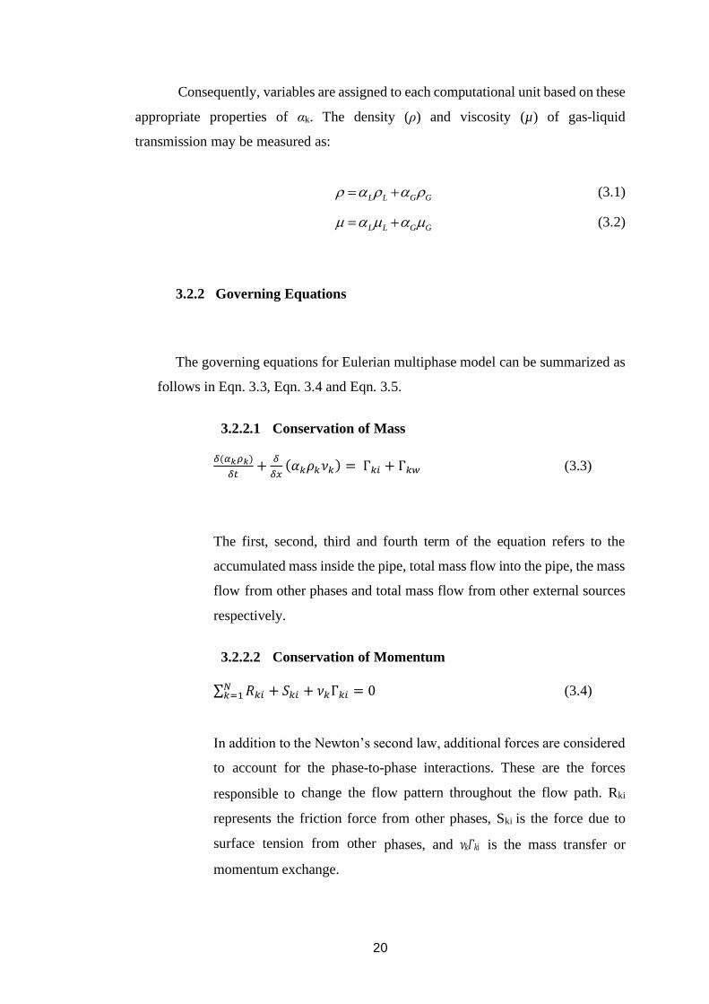
Consequently, variables are assigned to each computational unit based on these

appropriate properties of αk. The density (ρ) and viscosity (µ) of gas-liquid

transmission may be measured as:

L L G G = + (3.1)

L L G G = + (3.2)

3.2.2 Governing Equations

The governing equations for Eulerian multiphase model can be summarized as

follows in Eqn. 3.3, Eqn. 3.4 and Eqn. 3.5.

3.2.2.1 Conservation of Mass

𝛿(𝛼𝑘𝜌𝑘)

𝛿𝑡+

𝛿

𝛿𝑥(𝛼𝑘𝜌𝑘𝜈𝑘) = Г𝑘𝑖 + Г𝑘𝑤 (3.3)

The first, second, third and fourth term of the equation refers to the

accumulated mass inside the pipe, total mass flow into the pipe, the mass

flow from other phases and total mass flow from other external sources

respectively.

3.2.2.2 Conservation of Momentum

∑ 𝑅𝑘𝑖 + 𝑆𝑘𝑖 + 𝜈𝑘Г𝑘𝑖 = 0𝑁𝑘=1 (3.4)

In addition to the Newton’s second law, additional forces are considered

to account for the phase-to-phase interactions. These are the forces

responsible to change the flow pattern throughout the flow path. Rki

represents the friction force from other phases, Ski is the force due to

surface tension from other phases, and 𝜈𝑘𝛤𝑘i is the mass transfer or

momentum exchange.

21

3.2.2.3 Conservation of Energy

Considering all the internal and external energy sources acting on the

phases, the equation is given as:

𝛿

𝛿𝑡(𝛼𝑘𝐸𝑘 ) = −

𝛿

𝛿𝑥[𝛼𝑘𝜈𝑘(𝐸𝑘 + 𝑝𝑘)] + 𝑞𝑘𝑖 + 𝑞𝑘𝑤 + 𝑤𝑘𝑖

+ 𝑤𝑘𝑤 + Г𝑘𝑖ℎ𝑘𝑖 + Г𝑘𝑤ℎ𝑘𝑤

(3.5)

The first term represents the internal energy, q is the specific heat, w is

the specific work, Γ is the specific mass flow term, and h refers to the

specific enthalpy. The subscript “i” and “w” refers to the energy coming

from other phases and from outside to a phase k respectively.

3.2.3 k‒ε Turbulence Model

A Computational Fluid Dynamics (CFD) analysis was performed to test

number simulations of flux regimes in multiple flux phases, creating a fluid film

around a gas bubble and a cause of a slug creation of the flow. The improved

performance of the k-ε turbulence model was used for different reasons[6], to promote

the measurement of digital simulations; (1) the model was very straightforward in

format, in comparison to the other complex turbulent model; (2) a k-ε turbulence model

was a more general model, enabling a quantitative prediction of turbulent clock flow.

Many multiple facet flow research studies have demanded compatibility with k-р-

turbulence model of the non-slip boundary conditions of solid surfaces and of the wall

law in calls near solid surfaces (Yadav et al., 2014; De Schepper, 2008; Mazumder,

2012; Valleyet al., 2007; Cook and Kadri et al., 2011).

The two turbulence layer models were used to calculate the turbulent viscosity.

The whole computer area divided into a totally turbulent area was represented by a

distance near the turbulent Wall of the Reynolds in Eq. (3.6) a viscosity region.

22

Rek

= (3.6)

η is the normal cell center distance from the wall.

For a low Reynolds number, Reη < 200, the low Reynolds number k‒ε model

that was modified by Riverin et al. (2006) was used. Within FLUENT 16.1, the Jones

and Laimder model of RNG k‒ε 1972, was improved [18] which significantly

improved the accuracy of the turbulent model. This model has been used to avoid the

wall functions with the prevailing viscous force for the low Reynolds.

The regulative equations of k and its dissipation rate ε of turbulent fine energy

are defined as:

( ) ( ) T T

k k

Uk k k k

x y x x y y

+ = + + +

21 2

' 2T

kG

y

+ − −

(3.7)

2

1 1 2 2

( ) ( )'T

T T

UC f G C f

x y x x k k

+ = + + −

22

22 T TU

y y y

+ + +

(3.8)

k and ε is combined with the governing equations and the eddy viscosity relationship

is known as µT = ρCµk2/ε.

Development of Fluid Domain Model

The fluid model is essentially the hollow inner part of the pipe bend model.

Three cases of two-phase flow were studied, one using water & air and

another using crude oil & natural gas. The flow in the pipeline is the

23

combination of horizontal and vertical pipeline and is initialized as

stratified flow with initial volume fraction of 0.1 for air. Table 5 lists the

parameters of pipeline material which is ASTM Carbon Steel A106 GR B

as referred from ASME, Section II, Part D and Table 6 lists the boundary

conditions that will be used in the simulation.

Table 3.3.1: Pipeline parameters.

Parameters Value

Total Length 12 m

Pipe Diameter 80 mm

Bending Radius 120 mm

Density 7.8334e^-6 kg/mm2

Young’s Modulus 1.6608e^5 Mpa

Poisson’s Ratio 0.3

Bulk Modulus 1.384e^5 Mpa

Shear Modulus 63877 Mpa

Tensile Strength 414 Mpa

Yield Strength 241 Mpa

Table 3.3.2:Boundary Conditions

Boundary Conditions Remarks

Pipe Pressure Given along the whole pipe: 2.535 MPa

Standard Earth Gravity:

9.81 m/s2 being set downwards, - to Z axis. (- to X axis in ANSYS)

Pipe Temperature:

Given along the whole pipe

Referred to ISO DWG stating operating temp at 60°C

Pipe Idealization As input to software that pipe elbows are to be considered

Horizontal Force All horizontal sections of pipe, including 45° angled section: 569.37 N

Vertical Force All vertical sections of pipe, including 45° angle section: 569.37 N

Fluid Mass 10860.742 Kg as distributed load along the pipe. Value taken from pipe volume (11.818m3) and density of working fluid (919 kg/m3).

24

Meshing of Pipe and Fluid Domain

The meshing of the pipe (solid domain) and the fluid domain are meshed

separately each under ANSYS Transient Structural Module and ANSYS

CFX module. Both domains are meshed using sweep method with mixed

Quad/Tri elements and “Advanced Sizing Function” turned on at curvature.

Coarser mesh is used as a compromise to limited computational resources

and time. Table 3 lists the mesh properties difference between FEA and

CFD. The meshes are of good quality with aspect ratio well below the

recommended maximum aspect ratio of 18-20 by ANSYS documentation.

Figure 11 and Table 7 illustrate the mesh quality of both domains.

Figure 3.4.1: Mesh Of (A) Pipe Bend (B) Fluid Domain

Table 3.4.1: Difference in Mesh properties of FEA and CFD

Mesh Properties FEA CFD

No. of Elements 14122 65678

No. of Nodes 2112 15510

Max Aspect 6.22 13.24

Ratio (<100)

Max Skewness 0.80 0.53

(<1)

25

Modal Analysis

Modal analysis is performed in ANSYS Workbench to extract the natural

frequencies of the pipe structure under several constraints. Forced

vibrations if excited at the same frequency as the natural frequency,

resonance will occur and significant vibrations can happen. The natural

frequencies and its respective mode shapes are derived according to Eqn.

3.9.

[𝑀][Ü] + [𝐾][𝑈] = 0 (3.9)

Where, M is the mass matrix, U is the acceleration and K is the stiffness

matrix.

Screening Methodology

A modal analysis is first performed to extract the natural frequencies of the

pipe bend models for each of Case 1 and Case 2 using the Modal Analysis

module available in ANSYS Workbench.

Subsequently, the FSI simulations are performed to determine the flow-

induced vibration levels and are compared to the natural frequencies

extracted. Three locations of interests in the bend are monitored in the

simulations (Fig 12).

The first stage of screening is by using the fluctuations in volume fractions

of liquid in the fluid domain cross-section plane at the bend (colored in

green). The results are then verified with the FSI results in the solid

Figure 3.6.1: Locations monitored (At bend)

26

domain’s locations of interests, namely the point colored in red (monitors

displacement) and the cross-section plane colored in black (monitors Von

Mises Stress) as shown in Table 8. The screening method is in accordance

to the screening methodology proposed by Chica (2014).

Table 3.6.1: Properties measured at locations of interest

Location Properties monitored

Plane in Green Volume Fraction of Liquid

Plane in Black Von Mises Stress of Pipe

Red Dot Displacement of Pipe

27

Project Process Flow Chart

The project is conducted methodically based on the project process flow chart

as shown in Figure 13.

Figure 3.7.1: Project Flow Chart

28

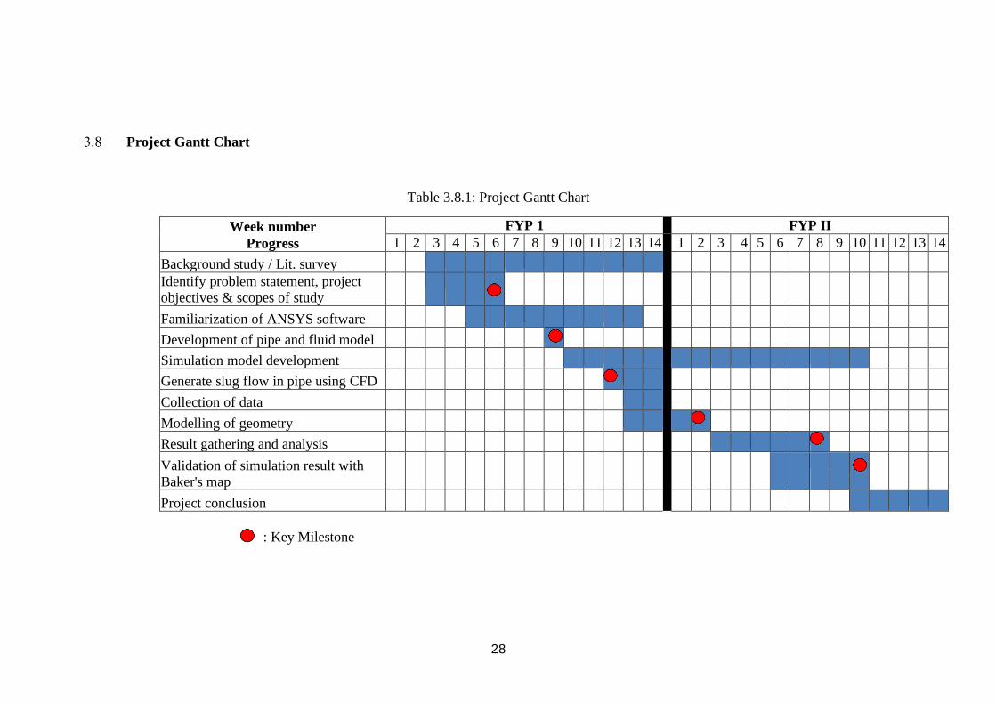
Project Gantt Chart

Table 3.8.1: Project Gantt Chart

Week number

Progress

FYP 1 FYP II

1 2 3 4 5 6 7 8 9 10 11 12 13 14

1 2 3 4 5 6 7 8 9 10 11 12 13 14

Background study / Lit. survey

Identify problem statement, project

objectives & scopes of study

Familiarization of ANSYS software

Development of pipe and fluid model

Simulation model development

Generate slug flow in pipe using CFD

Collection of data

Modelling of geometry

Result gathering and analysis

Validation of simulation result with

Baker's map

Project conclusion

: Key Milestone

29

RESULTS AND DISCUSSION

Validation of flow pattern on Baker’s map

Table 4.1.1: Simulation of the air-water operating condition for slug development.

G/λ (kgm-2s-1) G (kgm-2s-1) L λ ψ/G L (kgm-2s-1)

Slug 3 3 200 600

There is 5 flow pattern that was associated which are stratified flow pattern,

wavy flow pattern, slug flow pattern, annular flow pattern and bubble flow pattern.

However, this research focused on the slug development in pipeline and its effects on

pipe bend. The present simulation was observed and compared with the previous result

by De Schepper et al. (2008) and also experimental result by Mohmmed (2016). The

simulation conducted on the geometry of 8m horizontal long tube with 0.08m internal

diameter by using the VOF method.

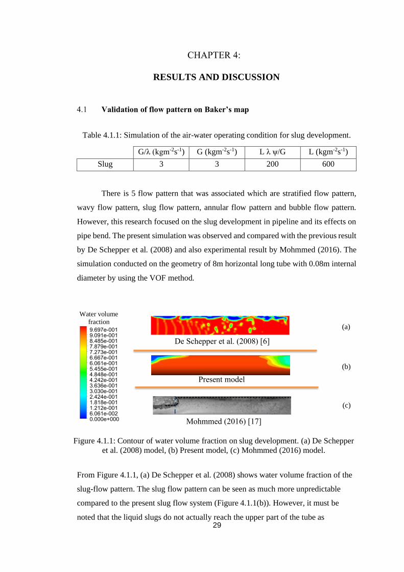
From Figure 4.1.1, (a) De Schepper et al. (2008) shows water volume fraction of the

slug-flow pattern. The slug flow pattern can be seen as much more unpredictable

compared to the present slug flow system (Figure 4.1.1(b)). However, it must be

noted that the liquid slugs do not actually reach the upper part of the tube as

(a)

(b)

(c)

Water volume

fraction

Present model

De Schepper et al. (2008) [6]

Mohmmed (2016) [17]

Figure 4.1.1: Contour of water volume fraction on slug development. (a) De Schepper

et al. (2008) model, (b) Present model, (c) Mohmmed (2016) model.

30

predicted from the Figure 4.1.1(c) observation. Note that the slug flow system is an

intermittent flow system, and the slug flow area is located in the center of the Baker

map (Figure 2.3.2). As described earlier, large transition zones can be present

between the different flow regimes. Because of these transition areas, the area

corresponding to the slug flow pattern for water – air flow may be very small relative

to the other flow pattern regions, which may explain the simulation results,

especially the difficulty of De Schepper et al. (2008) simulating a perfect slug flow

regime.

The experimental results are shown in slug flow from Figure 4.1.1 (c). For

this form of flow pattern also called intermittent flow where it occurs when the gas

velocity is the small and modest liquid velocity. Slug flow formation is due to

interface friction between water and air. The motion of the air mixture can come

from the flow of turbulence, or from the flow of stratified-wavy pattern. The bubbles

will migrate upward to the top of the pipe due to the buoyancy forces, and the

extended bubble will shape. The slug flow regime model proves the result of De

Schepper et al. (2008) and Mohmmed (2016) from the current results obtained.

The transition of slug flow pattern in a horizontal pipe

In the current situation, to identify the presence of slug flow are difficult

because of the properties of slug and its related criteria such as velocity, the formation

of slug and frequency. Figure 4.2 presented the formation of a slug at superficial

velocity, USG = 3.07 m/s and liquid superficial velocity USL = 0.4 m/s as in inlet

boundary condition. Along the pipe, the elongated bubble form is different in length

were some with small bubble gas throughout the pipe. The air bubble penetrates more

at slug front.

31

Figure 4.2.1: Water volume fraction contours of slug flow in the pipe.

The colour contour of red signifies liquid while blue refers to gas. The direction

flow for this figure is from left the inlet to the right towards the bend before the outlet.

The slug flow in the pipe can be clearly observe based on time evolution. The red

contour of liquid slug moving to the upper part of the horizontal pipe.

As of Figure 4.2.2, primarily the pipe was filled with an equal volume of air and

water with nil velocity. The mixture takes some time in simulation to ensure the

formation of the slug to occur as the first crest was formed. The formation of slug starts

to grow at time 0.5 second and then continue growing more along the pipe. The short

slug was observed from the contour at 1.0 second to 1.5 seconds. This turbulence was

taken from the current model and the formation of flow pattern can be observed when

the slug passes through the orifice plate geometry of 0.5 diameter ratio.

32

Figure 4.2.2: Time evolution contours of Slug flow and the water volume fraction

air-water towards the pipe’s elbow for (Usa = 3.07 m/s and Usw = 0.4 m/s).

Validation of model against Experimental figures

For this parts, the present model of CFD model simulation was used to

compare with the experimental result as for validation to guarantee the rightness and

assurance of current work. The prediction of CFD simulation was computed with an

experimental photograph.

4.3.1 The Experimental test methodology

For the previous validation of slug flow, it was validated based on the concept. For

this experimental test that been done by Dinaryanto et al. (2017) [16], it will be used

to compare with a present simulation model. The geometry of experimental test was

executed at 0.026 m of internal diameter and length of 10 m. Type of fluid used for

this type of experiment is air-water which are two-phase flow. The atmospheric

pressure, 101.3 kPa and room temperature, 24°C are been used respectively. From

Figure 4.3.1illustrate the schematic diagram of the experimental apparatus.

Flow direction

Water Volume

Fraction

2.0 s

2.5 s

3.0 s

3.5 s

4.0 s

To Pipe’s Elbow

33

Figure 4.3.1: The schematic diagram of the experimental apparatus [16].

4.3.2 CFD of slug development comparison between Experiment

photographs.

The following stage of slug formation between the current model simulation and

experimental snapshots are shown in Figure 4.3.2. Initially, the water volume fraction

of liquid and air are 50% as shown in Figure 4.3.2 (a) as the slug starts to initiate. As

been shown in Figure 4.3.2 (b) and (c), the red contour of water volume fraction shows

small crest develop the liquid hold up increase in form of slug liquid HLs = 0.55. When

the superficial velocity of the liquid set to 0.77 m/s, the thrust of the liquid increase

rapidly which causes the slug flow pattern to form and advanced along the pipe.

34

Figure 4.3.2: The evaluation of slug progression between experimental work and

CFD data simulation on water volume fraction for Usa = 1.88 m/s, Usw = 0.77 m/s (a)

Stratified pattern, (b) Crest jump and (c) slug pattern.

The assessment of slug flow pattern throughout the horizontal pipeline was

recorded between current work model from CFD simulation and experimental has

been presented in Figure 4.3.3. The inlet boundary condition for the slug in the pipe

are at USG = 1.88 m/s and USL = 0.77 m/s. From the experimental photographs and

water volume fraction, contour has been illustrated shows a strong and reasonable

comparison. The volume of fluid (VOF) method was used to obtain the water and air

boundary.

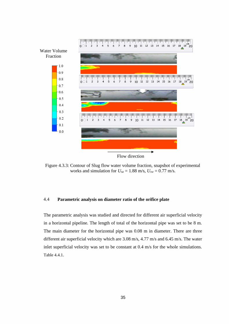
Figure 4.3.3 shows the slug flow region start to appear. According to the

experimental methodology, the picture of the slug flow pattern was taken based on

camera resolution of 1920 x 1080 with 1.20 m length. For Figure 4.3.3 the actual length

of 1-centimetre scale signified 0.034 meters. Thus, from the first picture taken shows

that the total slug length is 0.105 m as shown in Figure 4.3.3.

(a)

(c)

(b)

Water Volume

Fraction

Flow direction

35

Figure 4.3.3: Contour of Slug flow water volume fraction, snapshot of experimental

works and simulation for Usa = 1.88 m/s, Usw = 0.77 m/s.

Parametric analysis on diameter ratio of the orifice plate

The parametric analysis was studied and directed for different air superficial velocity

in a horizontal pipeline. The length of total of the horizontal pipe was set to be 8 m.

The main diameter for the horizontal pipe was 0.08 m in diameter. There are three

different air superficial velocity which are 3.08 m/s, 4.77 m/s and 6.45 m/s. The water

inlet superficial velocity was set to be constant at 0.4 m/s for the whole simulations.

Table 4.4.1.

Water Volume

Fraction

Flow direction

36

Table 4.4.1: The inlet boundary condition for parametric study.

Bending radius

over diameter of

pipe, r/D

Air inlet superficial

velocity, m/s

Water inlet superficial

velocity, m/s

1

3.08

0.4

4.77

6.45

1.5

3.08

4.77

6.45

3

3.08

4.77

6.45

4.4.1 Parametric analysis of air inlet superficial velocity on slug

development.

Since the volume of one phase cannot be substituted for the other

phases, the concept of the volume fraction is implemented. Such volume

fractions are called continuous space functions and are equivalent to one

number. For each point, conservation equations are derived in order to obtain a

set of equations with similar structures for all stages in order to validate the

superficial velocity principle.

37

Figure 4.4.1: Time record of water volume fraction on the cross sectional pipe

located before elbow when increases air superficial velocity from 3.08 m/s to 6.45

m/s with constant water superficial velocity, Usw = 0.4 m/s.

Table 4.4.2 shows the approximate time for slug to arrive at pipe’s elbow. When

superficial air velocity increased from 3.08 m/s to 6.45 m/s, the slug development

become faster. The contour of water volume fraction was tabulated in Table 4.4.3.

Table 4.4.2: Approximate time for Slug to arrive at pipe’s elbow.

Air inlet Superficial Velocity (m/s)

3.08 4.77 6.45

Time to form Slug (s) 7.4 6.2 4.5

Max Volume Fraction (-)

0.962 0.902 0.931

0

0.1

0.2

0.3

0.4

0.5

0.6

0.7

0.8

0.9

1

0 2 4 6 8 10

Wat

er V

olu

me

Frac

tio

n

Flow-time (s)

Water Volume Fraction vs Flow-time

Usg=3.08 m/s

Usg=4.77 m/s

Usg=6.45 m/s

38

Table 4.4.3: Water volume fraction contour on slug development for each condition

of air inlet superficial velocity

Air Superficial

Velocity (m/s) Water Volume Fraction (-)

3.08

0.962

4.77

0.902

6.45

0.931

39

(b)

(a)

4.4.2 Parametric analysis of air inlet superficial velocity towards exerted

pressure on the wall of the elbow.

According to Baker’s flow regime maps, there are specific ranges of inlet air

and water superficial velocity of a pipeline for various pattern of flow regimes. This

research focused on the study of slug flow pattern and its effects towards the elbow of

pipeline. Figure 4.4.2.

0

10000

20000

30000

40000

50000

60000

2 3 4 5 6 7 8

Pre

ssu

re (

Pa)

Inlet Air Superficial Velocity (m/s)

Pressure vs Inlet Air Superficial Velocity

0

10000

20000

30000

40000

50000

60000

2 3 4 5 6 7 8

Pre

ssu

re (

Pa)

Inlet Air Superficial Velocity (m/s)

40

(c)

(d)

Figure 4.4.2: The total exerted pressure on elbow’s wall against air inlet superficial

velocity with r/D ratio from 1.0 to 3.0 for graph (a) (b) (c) (d) with constant inlet Usw

= 0.4 m/s.

Figure 4.4.2 above shows the graph of total pressure against the air inlet superficial

velocity for slug flow that passes through the 90° elbow of the pipe with varies bending

radius over pipe diameter ratio of 1.0,1.5 and 3.0. The point data were plot by making

inlet superficial velocity of the air as manipulating variable from 3.08 m/s to 6.45 m/s

whereas water inlet superficial velocity as a constant variable for case (a) (b) (c) and

(d) which is USL = 0.4 m/s. The result concludes that the higher the air inlet superficial

velocity will produce a higher total pressure exerted on the inner part of pipe elbow.

Further study on the parameter analysis of pipe bending radius overe pipe diameter

ratio, r/D has been done in this research to analyse the effect of r/D ratio to the total

0

5000

10000

15000

20000

25000

30000

35000

40000

45000

2 3 4 5 6 7 8

Pre

ssu

re (

Pa)

Inlet Air Superficial Velocity (m/s)

0

10000

20000

30000

40000

50000

60000

2 3 4 5 6 7 8

Pre

ssu

re (

Pa)

Inlet Air Superficial Velocity (m/s)

r/D=1 r/D=1.5 r/D=3

41

(a)

(b)

(c)

pressure exerted on the inner part of pipe elbow. Figure shows the relations on the

parameter studied for this analysis.

0

5000

10000

15000

20000

25000

0 0.5 1 1.5 2 2.5 3 3.5 4

Pre

ssu

re (

Pa)

r/D (-)

Pressure vs r/D

Usg=3.08 m/s

0

5000

10000

15000

20000

25000

30000

35000

40000

0 0.5 1 1.5 2 2.5 3 3.5 4

Pre

ssu

re (

Pa)

r/D (-)

Usg=4.77 m/s

0

10000

20000

30000

40000

50000

60000

0 0.5 1 1.5 2 2.5 3 3.5 4

Pre

ssu

re (

Pa)

r/D (-)

Usg=6.45 m/s

42

(d)

Figure 4.4.3: The total exerted pressure on elbow’s wall against r/D ratio with air

inlet superficial velocity from 3.07 m/s to 6.45 m/s for graph (a) (b) (c) (d) with

constant inlet Usw = 0.4 m/s.

Table 4.4.4 displays the absolute pressure contour on two specific locations on the pipe

which are located at the beginning and the end of the pipe elbow which was defined

as Measurement Section 1 and Measurement Section 2 (refer to pipe geometry model).

The result concludes that the higher the air inlet superficial velocity will produce a

higher pressure drop across the pipe elbow. However, a significant higher-pressure

drop can be observed based on the result when decreasing the bending radius over pipe

diameter ratio, r/D.

0

10000

20000

30000

40000

50000

60000

0 0.5 1 1.5 2 2.5 3 3.5 4

Pre

ssu

re (

Pa)

r/D (-)

Usg=3.08 m/s Usg=4.77 m/s Usg=6.45 m/s

43

Table 4.4.4: Pressure Contour at Measurement Section 1 and 2 with varies value of

r/D ratio and air superficial velocity at constant inlet Usw = 0.4 m/s.

Absolute Pressure Contour

Location r/D Air: 3.08 m/s Air: 4.77 m/s Air: 6.45 m/s

Measu

remen

t Sectio

n 1

1.0

Pmax = 191.63 kPa Pmax = 193.31 kPa Pmax = 195.28 kPa

1.5

Pmax = 191.27 kPa Pmax = 194.74 kPa Pmax = 195.93 kPa

3.0

Pmax = 191.82 kPa Pmax = 193.21 kPa Pmax = 196.17 kPa

Absolute Pressure Contour

Location r/D Air: 3.08 m/s Air: 4.77 m/s Air: 6.45 m/s

Measu

remen

t Sectio

n 2

1.0

Pmax = 185.94 kPa Pmax = 187.27 kPa Pmax = 190.39 kPa

1.5

Pmax = 188.45 kPa Pmax = 190.83 kPa Pmax = 192.72 kPa

44

(b)

(a)

3.0

Pmax = 189.87 kPa Pmax = 192.52 kPa Pmax = 194.34 kPa

4.4.3 Parametric analysis of air inlet superficial velocity and r/D ratio on

resultant force exerted on the inner part of pipe elbow.

0

20

40

60

80

100

120

140

0 0.5 1 1.5 2 2.5 3 3.5

Forc

e (N

)

r/D

Force vs r/D

Usg=3.08 m/s

0

50

100

150

200

0 0.5 1 1.5 2 2.5 3 3.5

Forc

e (N

)

r/D

Force vs r/D

Usg=4.77 m/s

45

(c)

(d)

Figure 4.4.4: The resultant force on elbow’s wall against r/D ratio with air inlet

superficial velocity from 3.08 m/s to 6.45 m/s for graph (a) (b) (c) (d) with constant

inlet Usw = 0.4 m/s.

Based on Figure 4.10 shows the graph of resultant force on the inner part of pipe elbow

against the bending radius over pipe diameter ratio, r/D for slug flow that passes

through the 90° pipe elbow with a r/D ratio of 1.0, 1.5 and 3.0. The point data were

plotted by making inlet superficial velocity of the air as manipulating variable from

3.08 m/s to 6.45 m/s whereas water inlet superficial velocity as a constant variable for

case (a) (b) (c) and (d) USL = 0.4 m/s. The result concludes that the higher the bending

radius over pipe diameter ratio, r/D will produce a lower resultant force exerted on the

inner part of pipe elbow while higher air inlet superficial velocity results in lower

resultant force acted on the inner part on the pipe elbow.

0

50

100

150

200

250

300

0 0.5 1 1.5 2 2.5 3 3.5

Forc

e (N

)

r/D

Force vs r/D

Usg=6.45 m/s

0

50

100

150

200

250

300

0 0.5 1 1.5 2 2.5 3 3.5

Forc

e (N

)

r/D

Force vs r/D

Usg=3.08 m/s Usg=4.77 m/s Usg=6.45 m/s

46

CONCLUSIONS AND RECOMMENDATIONS

Pipelines work as a transport medium in transporting medium among or more

remote stations. Fluid flow pattern inside horizontal pipes consists of gas and liquid

happened in the production of fuel and gas industry. Piping is the common medium

for these types of industry to transport the liquid. Horizontal bending pipe geometry

has been selected as a research parameter to correlate the bending radius over pipe

diameter ratio, r/D to the resulting level of flow induced vibration arising from slug

flow in the pipe. For these researches, volume of fluid (VOF) method was used where

it is the model that is able to produce excellent surface result simulation for slug flow.

Air and water were selected as an operating condition for these projects in the

horizontal pipe.

The validation result of the present model of flow regime is equivalent to the

research paper from De Schepper [6] that refer to the Baker’s flow regime map. The

simulation was done for the present model use the VOF method. Moreover, the present

work obtained a similar slug flow pattern in the horizontal pipe. The research then

covers the r/D ratio with different r/D values in a horizontal bending pipeline. In

addition, the slug development become faster when superficial velocity increased from

3.08 m/s to 6.45 m/s as possibly due to the increase of likely turbulence flow in the

pipe. The slug that was developed in the pipe was indicated by the reading of the flow

water volume fraction which was equally to the value of nearest to 1.

It can be concluded that the pressure exerted on the inner part of pipe elbow

increases when the inlet superficial velocity of air increases while the higher the value

of r/D of a pipe will results in a lower pressure exerted on the inner part of an elbow.

Due to the sudden change of the direction of the flow, the slug that was developed in

the pipe produces a high-pressure impact on the inner part of the pipe elbow which

was also interpreted as the high resultant force exerted on the inner part of the elbow’s

wall. This high resultant force will then be causing a vibration phenomenon on the

wall of the pipe and the main cause for this vibration is highly related to the differential

pressure (pressure loss) which occurs across the elbow of the pipe.

47

As part of the recommendation, future works for improvement that could be

done in the future are by furthering the research to three-phase flow that considered

oil, gas, and water in the simulation. The studies will be similar to the baker’s map

flow regime. Other than that, use a vertical bending pipe with various bending angles

such as 45°, 135° and U-shaped pipe bend as the parametric study to observe the effect

of pipe bend angle to the resulting level of induced vibration on the pipe. Finally, use

more data point to obtain a better trend for the results.

48

REFERENCES

[1] K. Havre, K.O. Stornes and H. Stray. (2000, April). Taming slug flow in

pipelines. [Online]. Available:

http://www02.abb.com/global/seitp/seitp161.nsf/viewunid/8A01902E860EAE

9185256B57006D9803/$file/ABBReview2000.pdf

[2] W. Peng and X. Cao, “Numerical simulation of solid particle erosion in pipe

bends for liquid–solid flow,” Powder Technology, vol. 294, pp. 266-279,

2016.

[3] D. H. Kim and S. H. Chang, “Flow-induced vibration in two-phase flow with

wire coil inserts” International Journal of Multiphase Flow, vol. 34, (4), pp.

325-332, 2008.

[4] B. L. Tay and R. B. Thorpe, “Effects of liquid physical properties on the

forces acting on a pipe bend in gas–liquid slug flow,” Chemical engineering

research and design, vol. 82, (3), pp. 344-356, 2004

[5] M. S. Yadav, T. Worosz, S. Kim, K. Tien and S. M. Bajorek,

“Characterization of the dissipation of elbow effects in bubbly two-phase

flows,” International Journal of Multiphase Flow, vol. 66, pp. 101-109, 2014.

[6] S. C. De Schepper, G. J. Heynderickx and G. B. Marin, “CFD modeling of all

gas–liquid and vapor–liquid flow regimes predicted by the Baker chart,”

Chemical Engineering Journal, vol. 138, (1-3), pp. 349-357, 2008.

[7] L. Chica, “Fluid Structure Interaction Analysis of Two-Phase Flow in an M-

shaped Jumper,” in Star Global Conference 2012, University of Houston,

Houston, United States, 2012.

[8] Q.H. Mazumder, “CFD Analysis of the Effect of Elbow Radius on Pressure

Drop in Multiphase Flow,” University of Michigan-Flint, USA, 2012.

49

[9] C. Vallee, H. Hohne, H.M. Prasser and T. Suhnel, “Experimental

Investigation and CFD Simulation of Horizontal Stratified Two-phase Flow

Phenomena,” Forschungszentrum Rossendrof e. V., Dresden, Germany. 2007.

[10] Y. Liu, S. Miwa, T. Hibiki, M. Ishii, H. Morita, Y. Kondoh, et al.,

"Experimental study of internal two-phase flow induced fluctuating force on a

90° elbow," Chemical Engineering Science, vol. 76, pp. 173-187, 2012.

[11] U. Kadri, R. Henkes, R. Mudde, and R. Oliemans, "Effect of gas pulsation on

long slugs in horizontal gas–liquid pipe flow," International journal of

multiphase flow, vol. 37, pp. 1120-1128, 2011.

[12] J.L. Riverin and M. Pettigrew, "Vibration excitation forces due to two-phase

flow in piping elements," Journal of Pressure Vessel Technology, vol. 129,

pp. 7-13, 2007.

[13] J. Riverin, E. De Langre, and M. Pettigrew, "Fluctuating forces caused by

internal two-phase flow on bends and tees," Journal of sound and vibration,

vol. 298, pp. 1088-1098, 2006.

[14] Z. I. Al-Hashimy, H. H. Al-Kayiem, R. W. Time, and Z. K. Kadhim,

"Numerical Characterisation of Slug Flow in Horizontal Air/water Pipe

Flow," International Journal of Computational Methods and Experimental

Measurements, vol. 4, pp. 114-130, 2016.

[15] H. Abdulmouti, “Bubbly two-phase flow: Part I-characteristics, structures,

behaviors and flow patterns,” American Journal of Fluid Dynamics,vol. 4,

(4), 194-240. 2014.

[16] O. Dinaryanto, Y. A. K. Prayitno, A. I. Majid, A. Z. Hudaya, Y. A.

Nusirwan, A. Widyaparaga, Indarto and Deendarlianto, “Experimental

investigation on the initiation and flow development of gas-liquid slug two-

phase flow in a horizontal pipe,” Experimental Thermal and Fluid Science,

vol. 81, pp. 93-108, 2017.

50

[17] A. O. Mohmmed, "Effect of slug two-phase flow on fatigue of pipe material,"

Ph.D Dissertation, Department of Mechanical Engineering, Universiti

Teknologi PETRONAS, Malaysia. 2016

[18] Z. I. Al-Hashimy, H. H. Al-Kayiem and R. W. Time, “Experimental

investigation on the vibration induced by slug flow in horizontal pipe,” ARPN

J. Eng. Appl. Sci, vol. 11, pp. 12134-12139, 2016.

[19] D. Q. Hou, A. S. Tijsseling, and Z. Bozkus, “Dynamic force on an elbow

caused by a traveling liquid slug,” Journal of Pressure Vessel Technology,

vol. 136, (3), 2014.

[20] S. Miwa, M. Mori and T. Hibiki, “Two-phase flow induced vibration in

piping systems,” Progress in Nuclear Energy, vol. 78, pp. 270-284, 2015.