Computability Tao Jiang Department of Computer Science McMaster University Hamilton, Ontario L8S 4K1, Canada Ming Li Department of Computer Science University of Waterloo Waterloo, Ontario N2L 3G1, Canada Bala Ravikumar Department of Computer Science University of Rhode Island Kingston, RI 02881, USA Kenneth W. Regan Department of Computer Science State University of New York at Buffalo Buffalo, NY 14260, USA 1 Introduction In the last two chapters, we have introduced several important computational models, including Turing machines, and Chomsky’s hierarchy of formal grammars. In this chapter, we will explore the limits of mechanical computation as defined by these models. We begin with a list of fundamental problems for which automatic computational solution would be very useful. One of these is the universal simulation problem : can one design a single algorithm that is capable of simulating any algorithm? Turing’s demonstration that the answer is yes [Turing, 1936] supplied the proof for Babbage’s dream of a single machine that could be programmed to carry out any computational task. We introduce a simple Turing machine programming language called “GOTO” in order to facilitate our own design of a universal machine. Next, we describe the schemes of primitive recur- sion and μ-recursion , which enable a concise, mathematical description of computable functions that is independent of any machine model. We show that the μ-recursive functions are the same as those computable on a Turing machine, and describe some computable functions including one that solves a second problem on our list. The success in solving ends there, however. We show in the last section of this chapter that 1

Welcome message from author
This document is posted to help you gain knowledge. Please leave a comment to let me know what you think about it! Share it to your friends and learn new things together.
Transcript
Computability
Tao Jiang
Department of Computer Science
McMaster University
Hamilton, Ontario L8S 4K1, Canada
Ming Li
Department of Computer Science
University of Waterloo
Waterloo, Ontario N2L 3G1, Canada
Bala Ravikumar
Department of Computer Science
University of Rhode Island
Kingston, RI 02881, USA
Kenneth W. Regan
Department of Computer Science
State University of New York at Buffalo
Buffalo, NY 14260, USA
1 Introduction
In the last two chapters, we have introduced several important computational models, including
Turing machines, and Chomsky’s hierarchy of formal grammars. In this chapter, we will explore the
limits of mechanical computation as defined by these models. We begin with a list of fundamental
problems for which automatic computational solution would be very useful. One of these is the
universal simulation problem: can one design a single algorithm that is capable of simulating any
algorithm? Turing’s demonstration that the answer is yes [Turing, 1936] supplied the proof for
Babbage’s dream of a single machine that could be programmed to carry out any computational
task. We introduce a simple Turing machine programming language called “GOTO” in order to
facilitate our own design of a universal machine. Next, we describe the schemes of primitive recur-
sion and µ-recursion, which enable a concise, mathematical description of computable functions
that is independent of any machine model. We show that the µ-recursive functions are the same
as those computable on a Turing machine, and describe some computable functions including one
that solves a second problem on our list.
The success in solving ends there, however. We show in the last section of this chapter that
1

all of the remaining problems on our list are unsolvable by Turing machines, and subject to the
Church-Turing thesis, have no mechanical or human solver at all. That is to say, there is no Turing
machine or physical device, no stand-alone product of human invention, that is capable of giving
the correct answer to all—or even most—instances of these problems. The implication we draw is
that in order to solve some important instances of these problems, human ingenuity is needed to
guide powerful computers down the paths felt most likely to yield the answers. To cite Raymond
Smullyan quoting P. Rosenbloom, the results on unsolvability imply that “man can never eliminate
the necessity of using his own cleverness, no matter how cleverly he tries.”
Almost the first consequence of formalizing computation was that we can formally establish its
limits. Kurt Godel showed that the process of proof in any formal axiomatic system of logic can
be simulated by the basic arithmetical functions that computation is made of. Then he proved
that any sound formal system that is capable of stating the grade-school rules of arithmetic can
make statements that can be neither be proved nor disproved in the system. Put another way,
every sound formal system is incomplete in the sense that there are mathematical truths that
cannot be proved in the system. Turing realized that Godel’s basic method could be applied to
computational models themselves, and thus proved the first computational unsolvability results.
Since then, problems from many areas, including group theory, number theory, combinatorics, set
theory, logic, cellular automata, dynamical systems, topology, and knot theory, have been shown
to be unsolvable. In fact, proving unsolvability is now an accepted “solution” to a problem. It is
just a way of saying that the problem is too general for a computer to handle—that supplementary
information is needed to enable a mechanical solution.
Since Turing machines capture the power of mechanical computability, our study will be based
on Turing’s model. In the next section, we describe a Turing machine as a computer that can
run programs written in a very simple language we call the “GOTO Language.” This formalism is
equivalent to Chapter 30’s description of Turing machines using the standard 7-tuple notation. Our
language provides an alternate way to write programs and makes proofs about Turing machines
more intuitive.
2
2 Computability and a Universal Program
Turing’s notion of mechanical computation was based on identifying the basic steps in any mechan-
ical computation. He reasoned that an operation such as numerical multiplication is not primitive,
because it can be divided into simpler steps such as using the times-table on individual pairs of dig-
its, shifting, and adding. Addition itself can be broken down into simpler steps such as adding the
lowest digits, computing the carry, and moving to the next digit. Turing concluded that the most
basic features of mechanical computation are the ability to read and write on a storage medium,
the ability to move about on that medium, and the ability to make simple logical decisions. Turing
chose the storage medium to be a single linear tape divided into cells. He showed that such a tape
could model spatial memory in three (or any number of) dimensions through the use of indexed
co-ordinates. With much care he argued that human sensory input could be encoded by strings
over a finite alphabet of cell symbols called the tape alphabet . (This bold discretization of sensory
experience now seems a harbinger of the digital revolution that was to follow.) A decision step
enables the computer to exert local control over the sequence of actions. Turing restricted the
next action performed to be in a cell neighboring the one on which the current action occurred,
and showed how non-local actions can be simulated by successions of steps of this kind. He also
introduced an instruction to tell the computer to stop.
In summary, Turing proposed a model to characterize mechanical computation as being carried
out as a sequence of instructions. Our “GOTO” formalism provides the following five kinds of
instructions. Here i stands for a tape symbol and j stands for a line number.
PRINT i
MOVE RIGHT
MOVE LEFT
IF i IS SCANNED GOTO LINE j
STOP
When we speak about programs recognizing languages rather than computing functions, we replace
STOP by statements ACCEPT and REJECT, each of which need occur only once in a program.
A program in this language is a sequence of instructions or “lines” numbered 1 to k. The input
to the program is a string over a designated input alphabet Σ, which we take to be {0, 1} throughout
3

this chapter. The tape alphabet includes Σ and a special blank character B representing an empty
cell, and may (but need not) contain other symbols. The input is stored on the tape, with the read
head scanning the first symbol (or B if the input is empty), before the computation begins.
How much memory should we allow the computer to use? Rather than postulate that the tape
is actually infinite—an unrealistic assumption—we prefer here to say that the tape has expandable
boundaries. Initially the input defines the two boundaries of the tape. Whenever the machine
moves left of the left boundary or right of the right boundary, a new memory cell containing the
blank is attached. This convention clarifies what we mean by saying that if and when the machine
halts by reaching the STOP instruction, the “result” of the computation is the entire content of
the tape.
We present an example program written in the GOTO language. This program accomplishes
the simple task of doubling the number of initial 1s in the input string. Informally, the program
achieves its goal as follows: When it reads a 1, it changes the 1 to a 0, moves left looking for a new
cell, and writes a 1 in that cell. Then it returns rightward to the 0 that marks where it had been,
rewrites it as a 1, and moves right to look for more 1s. If it immediately finds another 1 it repeats
the process from line 1, while if it doesn’t, it halts right there. This program even has a “bug”—it
“should” leave strings that do not begin with a 1 unchanged, but instead it alters them.
The main change from the traditional Turing machine formalism of Chapter 30 is that we have
replaced “states” by line numbers. A Turing machine of the former kind can always be simulated
in our GOTO language by making blocks of successive lines, themselves divided into sub-blocks for
each character that are headed by “IF” statements, carry out the instructions for each state. Our
formalism makes many programs more succinct and closer to programmers’ experience, and high-
lights the role of (conditional) GOTO instructions in setting up loops and enabling statements to be
repeated. Despite the popular scorn of goto statements, this feature is ultimately the most impor-
tant aspect of programming and can be found in every imperative-style programming language—at
least in the code produced by the compiler if the language has no goto instruction itself. Indeed,
the above example could be rendered into a structured programming language such as C as follows,
do {
do { PRINT 0; MOVE LEFT; } while (1 is scanned);
4

1 PRINT 0
2 MOVE LEFT
3 IF 1 IS SCANNED GOTO LINE 2
4 PRINT 1
5 MOVE RIGHT
6 IF 1 IS SCANNED GOTO LINE 5
7 PRINT 1
8 MOVE RIGHT
9 IF 1 IS SCANNED GOTO LINE 1
10 STOP
Figure 1: The doubling program in the GOTO language.
PRINT 1;
do MOVE RIGHT; while (1 is scanned);
PRINT 1; MOVE RIGHT; }
while (1 is scanned);
and a C compiler (using a character array tape[i] and ++i, --i for the moves) might plausibly
convert this into something exactly like our GOTO program!
The simplicity of the GOTO language is rather deceptive. As the above example hints, any
program in any known high-level programming language can be converted into an equivalent GOTO
program, under suitable conventions on how inputs and outputs are represented on the tape. (If
the program only reads from the standard input stream and writes to the standard output stream,
then no such conventions are necessary.) There is strong reason to believe that any mechanical
computation of any future kind can be expressed by a suitable GOTO program. Note, however,
that a program written in the GOTO language need not always halt; i.e., on certain inputs the
program may never reach a STOP instruction. On such inputs we say that the output of the
program is undefined .
Now we can give a precise definition of what we mean by an algorithm, attempting to rule
5

out this last situation. An algorithm is any program written in the GOTO language that has the
additional property of halting on all inputs. Such programs will be called halting programs, and
correspond to “total” deterministic Turing machines in Chapter 30. When we consider decision
problems, which have yes/no answers, halting programs are required to end their computation with
either an ACCEPT or a REJECT statement, on any input.
2.1 Some Computational Problems
We begin by listing a collection of computational problems for which a mechanical solution can be
very helpful. By a mechanical solution, we mean a step-by-step process that takes into account all
possible inputs, and that can be executed without any human assistance once a certain input is
provided. An algorithm is required to work correctly on all instances.
We now list some problems that are fundamental either because they are inherently important
or because they played a historical role in the development of computation theory. For the first
four, P stands for a program in our GOTO language, and x is a string over the input alphabet,
which we fix to be {0, 1}.
1. Universal simulation. Given a program P and an input x to P , determine the output (if any)
that P would produce on input x.
2. Halting problem. Given P and x, output 1 (for yes) if P would halt when given input x, and
0 (for no) if P would not halt.
3. Type-0 grammar membership. Given a type-0 grammar G and a string x, determine whether
x can be derived from the start symbol of G.
4. String compression. Given a string x, find the shortest program P such that when P is started
with empty tape, P eventually halts with x as its output. Here “shortest” means that the
total number of symbols in the program’s instructions is as small as possible.
5. Tiling. Given a finite set T of tile types, where all tiles of a type are unit squares with the
same four colors on their four edges, determine whether every finite rectangle can be tiled by
T . If k and n are the integer sides of the rectangle, being tiled means that kn tiles drawn
6
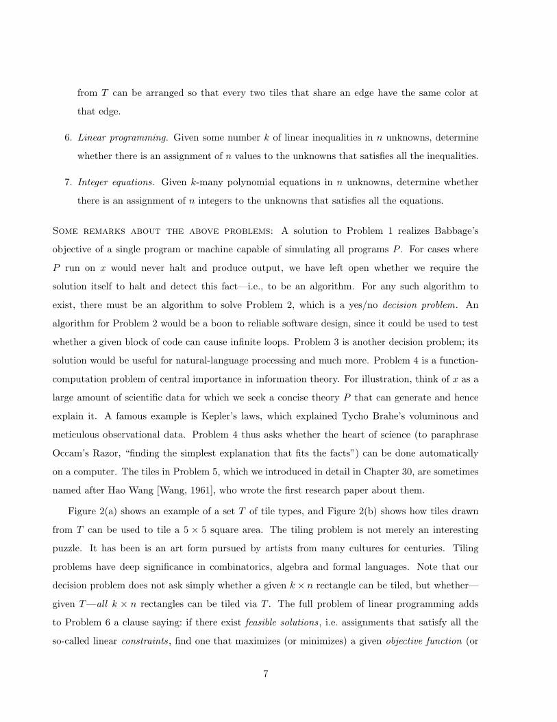
from T can be arranged so that every two tiles that share an edge have the same color at
that edge.
6. Linear programming. Given some number k of linear inequalities in n unknowns, determine
whether there is an assignment of n values to the unknowns that satisfies all the inequalities.
7. Integer equations. Given k-many polynomial equations in n unknowns, determine whether
there is an assignment of n integers to the unknowns that satisfies all the equations.
Some remarks about the above problems: A solution to Problem 1 realizes Babbage’s
objective of a single program or machine capable of simulating all programs P . For cases where
P run on x would never halt and produce output, we have left open whether we require the
solution itself to halt and detect this fact—i.e., to be an algorithm. For any such algorithm to
exist, there must be an algorithm to solve Problem 2, which is a yes/no decision problem. An
algorithm for Problem 2 would be a boon to reliable software design, since it could be used to test
whether a given block of code can cause infinite loops. Problem 3 is another decision problem; its
solution would be useful for natural-language processing and much more. Problem 4 is a function-
computation problem of central importance in information theory. For illustration, think of x as a
large amount of scientific data for which we seek a concise theory P that can generate and hence
explain it. A famous example is Kepler’s laws, which explained Tycho Brahe’s voluminous and
meticulous observational data. Problem 4 thus asks whether the heart of science (to paraphrase
Occam’s Razor, “finding the simplest explanation that fits the facts”) can be done automatically
on a computer. The tiles in Problem 5, which we introduced in detail in Chapter 30, are sometimes
named after Hao Wang [Wang, 1961], who wrote the first research paper about them.
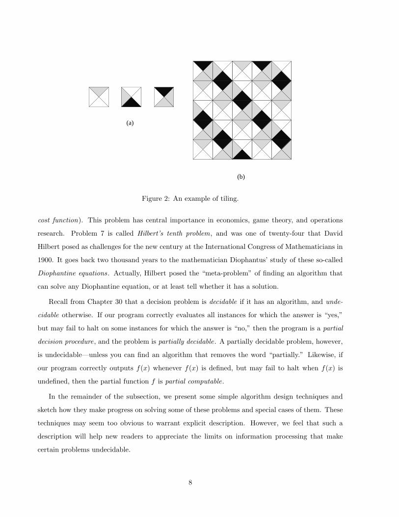
Figure 2(a) shows an example of a set T of tile types, and Figure 2(b) shows how tiles drawn
from T can be used to tile a 5 × 5 square area. The tiling problem is not merely an interesting
puzzle. It has been is an art form pursued by artists from many cultures for centuries. Tiling
problems have deep significance in combinatorics, algebra and formal languages. Note that our
decision problem does not ask simply whether a given k × n rectangle can be tiled, but whether—
given T—all k × n rectangles can be tiled via T . The full problem of linear programming adds
to Problem 6 a clause saying: if there exist feasible solutions, i.e. assignments that satisfy all the
so-called linear constraints, find one that maximizes (or minimizes) a given objective function (or
7
(a)
(b)
Figure 2: An example of tiling.
cost function). This problem has central importance in economics, game theory, and operations
research. Problem 7 is called Hilbert’s tenth problem, and was one of twenty-four that David
Hilbert posed as challenges for the new century at the International Congress of Mathematicians in
1900. It goes back two thousand years to the mathematician Diophantus’ study of these so-called
Diophantine equations. Actually, Hilbert posed the “meta-problem” of finding an algorithm that
can solve any Diophantine equation, or at least tell whether it has a solution.
Recall from Chapter 30 that a decision problem is decidable if it has an algorithm, and unde-
cidable otherwise. If our program correctly evaluates all instances for which the answer is “yes,”
but may fail to halt on some instances for which the answer is “no,” then the program is a partial
decision procedure, and the problem is partially decidable. A partially decidable problem, however,
is undecidable—unless you can find an algorithm that removes the word “partially.” Likewise, if
our program correctly outputs f(x) whenever f(x) is defined, but may fail to halt when f(x) is
undefined, then the partial function f is partial computable.
In the remainder of the subsection, we present some simple algorithm design techniques and
sketch how they make progress on solving some of these problems and special cases of them. These
techniques may seem too obvious to warrant explicit description. However, we feel that such a
description will help new readers to appreciate the limits on information processing that make
certain problems undecidable.
8

2.1.1 Table Look-up
For certain functions g it can be advantageous to create a table with one column for inputs x and
one for values g(x), looking up the value in the table whenever an evaluation g(x) is needed. A
function f that is defined on an infinite set such as Σ∗ cannot have its values enumerated in a
finite table in this manner, but sometimes the infinite table for f can be described in a finite way
that constitutes an algorithm for f . Moreover, tables for other functions g may help the task of
computing f , such as the digit-by-digit times-table used in multiplying integers of arbitrary size.
These ideas come into play next.
2.1.2 Bounding the Search Domain
Many solutions to decision problems involve finding a witness that proves a “yes” or “no” answer
for a given instance. The term reflects an analogy to a criminal trial where a key witness may
determine the guilt or innocence of the defendant. Thus the first step in solving many decision
problems is to identify the right kind of witness to look for. For example, consider the problem of
determining whether a given number N is prime. Here a (counter-) witness would be a factor of
N (other than 1 and N itself). If N is composite, it is easy to prove by simple division that the
witness’ claim is correct.
In cases where the given number is prime, a witness of a different kind needs to be searched for.
This search may involve integers larger than N , and trying to summon every integer sequentially as
a witness would violate the requirement of an algorithm to terminate in finite number of steps. This
is often the main challenge in establishing decidability. The difficulty can be surmounted if, based
on the structure of the problem, we can establish ahead of time an upper bound such that if any
witness exists at all, one exists that meets the bound. Then a sufficient body of potential witnesses
can be examined in a finite number of steps. In the case of composite N , the bound is N itself. For
prime N , there is a known polynomial p such that a witness exists in the numbers between 1 and
2p(n), where n is the number of digits in N , according to a certain witnessing scheme whose test
for correct claims is easy to compute. This kind of “polynomial size-bounded witnessing scheme”
characterizes the important complexity class NP, and is discussed much further in Chapter 33.
For another example, let us consider the special case of Problem 3 where the given G is a
9

Type-1 grammar, and we wish to determine whether a given string x can be generated from the
start symbol S of G. A witness in this case can be a sequence of sentential forms starting from S
and ending with x that forms a valid derivation in G. The length of x imposes a limit on the size
of such sentential forms because G has no length-decreasing productions, and this in turn defines a
(much larger) limit on the number of sequences that need be considered before all possibilities are
exhausted. Readers may find the details in a standard text such as [Hopcroft and Ullman, 1979].
For one more example, consider the full version of the linear programming problem where one
wishes to maximize a linear objective function f over the set of feasible solutions s. This set may
be infinite, and so a table-lookup through all values f(s) cannot be used. However, it is possible
to reduce the search domain to a finite set as follows. The feasible solutions form a collection
n-dimensional space, where n is the number of variables plus the number of constraints) known as
a convex polytope. Unless the polytope is empty or unbounded—cases that can be detected and
resolved—the polytope has a finite number of “corner” points, which are similar to the vertices
of a polygon, and which are easily computed. In this case, it is known that a linear objective
function attains its maximum value at one (or more) of these corner points. Thus we know the
problem is decidable via table-lookup of values at the corner points. In practice, there are intelligent
algorithms that find a maximum-giving corner point after searching (usually) only a small part of
this table.
2.1.3 Use of Subroutines
This is more a programming technique than an algorithm design tool. The idea is to use one
program P as a single step in another program Q. Building programs from simpler programs is
a natural way to deal with the complexity of the programmer’s task. A simple example is using
a lookup to the times table as a subroutine in multiplying two integers i and j. Let us examine
this in the context of designing Turing machines, where i and j are represented on the tape by the
string 1i01j (namely, i 1s followed by a 0 and then by j 1s). The basic idea of our GOTO program
is to duplicate the string of i 1s j − 1 times, meanwhile erasing the string 1j bit-by-bit to count
the iterations. A little thought reveals that our earlier GOTO program in Figure 2 can almost be
used verbatim as a subroutine to call j − 1 times. The only hitch is that the first call would run
2i-many 1s together so that further calls would duplicate too many 1s. To fix the problem, we
10

introduce a new tape symbol 2, using two initial steps to convert the tape to 21i01j , and “patch”
the subroutine so that it will not overwrite this 2. The new subroutine can be called by a line “k:
IF 2 IS SCANNED GOTO m,” where m is the number of the first line in the subroutine, and can
return control to the point of call by replacing its STOP instruction by “IF 0 IS SCANNED GOTO
k+ 1.” Careful writing will ensure that this latter 0 is the one initially separating 1i from 1j . The
remaining details are left to the interested reader, while performing a similar patch without using
a new symbol “2” is left to the obsessive reader. This subroutine mechanism is in fact no different
from the one programmers in BASIC have used for decades.
2.2 A Universal Program
We will now solve Problem 1 by arguing the existence of a program U written in the GOTO
language that takes as input a program P (also written in the GOTO language) and data x for P ,
and that produces the same output as P does on input x, if P (x) halts and produces output at
all. The last caveat hints that we shall only achieve a partial solution, formally showing only that
the function U(P, x) = P (x) is partial computable.
For convenience, we assume that all programs written in the GOTO language use the fixed
alphabet {0, 1, B}. Since we have thus far used the full English alphabet for the notation of our
GOTO programs, we must first address the issue of what the formal input to the program U will
look like. This problem can be circumvented by encoding each instruction using only 0 and 1. The
idea of such an encoding should not be mysterious—we could refer to the 0-1 encoding defined by
the ASCII standard, which the terminal used to type this chapter has already carried out for these
example programs. However, we prefer the more-succinct encoding defined by Table 1.
To encode an entire program, we simply write down in order (without the line numbers) the
code for each instruction as given in the table. For example, here is the code for the doubling
program shown in Figure 2:
0001001011110110001101001111111011000110100111011100.
Note that the encoded string preserves all the information about the program, so that one can easily
reverse the process to decode the string into a GOTO program. From now on, if P is a program in
the GOTO language, code(P ) will denote its binary encoding. When there is no confusion, we will
11
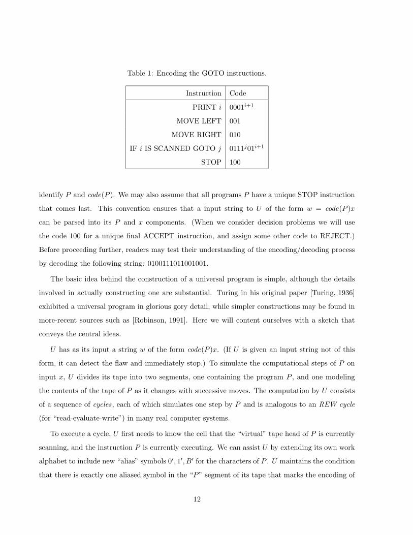
Table 1: Encoding the GOTO instructions.
Instruction Code
PRINT i 0001i+1
MOVE LEFT 001
MOVE RIGHT 010
IF i IS SCANNED GOTO j 0111j01i+1
STOP 100
identify P and code(P ). We may also assume that all programs P have a unique STOP instruction
that comes last. This convention ensures that a input string to U of the form w = code(P )x
can be parsed into its P and x components. (When we consider decision problems we will use
the code 100 for a unique final ACCEPT instruction, and assign some other code to REJECT.)
Before proceeding further, readers may test their understanding of the encoding/decoding process
by decoding the following string: 0100111011001001.
The basic idea behind the construction of a universal program is simple, although the details
involved in actually constructing one are substantial. Turing in his original paper [Turing, 1936]
exhibited a universal program in glorious gory detail, while simpler constructions may be found in
more-recent sources such as [Robinson, 1991]. Here we will content ourselves with a sketch that
conveys the central ideas.
U has as its input a string w of the form code(P )x. (If U is given an input string not of this
form, it can detect the flaw and immediately stop.) To simulate the computational steps of P on
input x, U divides its tape into two segments, one containing the program P , and one modeling
the contents of the tape of P as it changes with successive moves. The computation by U consists
of a sequence of cycles, each of which simulates one step by P and is analogous to an REW cycle
(for “read-evaluate-write”) in many real computer systems.
To execute a cycle, U first needs to know the cell that the “virtual” tape head of P is currently
scanning, and the instruction P is currently executing. We can assist U by extending its own work
alphabet to include new “alias” symbols 0′, 1′, B′ for the characters of P . U maintains the condition
that there is exactly one aliased symbol in the “P” segment of its tape that marks the encoding of
12

the current instruction, and exactly one in the other segment that marks the cell currently scanned
by P . For example, suppose that after thirty-nine steps, P is reading the fourth symbol from the
left on its tape containing 01001001. Then the second tape segment of U after thirty-nine cycles
consists of the string 0100′1001. We can further assist U by adding a symbol ∧ to divide the two
segments, although the unique STOP instruction itself could serve as the divider. The computation
by U on an input w = code(P )x can begin with some steps that prime the first symbol of code(P ),
insert a ∧ before the first symbol of x (caterpillaring x one cell to the right), and prime the first
symbol of x. We may suppose that each cycle by U begins with its own head scanning the ∧.
At the beginning of a new cycle, U moves its head left to find the current instruction, and
begins decoding it. The only information U needs to retain is which type of instruction it is, and in
the case of a PRINT i or IF i. . . instruction, which character i is involved. To execute a PRINT i,
MOVE RIGHT, or MOVE LEFT instruction, P unprimes the instruction, primes the next one,
and marches down its tape to find the primed cell on its copy of P ’s tape and execute the action. It
is possible that a MOVE LEFT instruction may bump into the ∧, in which case U makes another
call to its “caterpillar” subroutine to move P ’s tape over, and inserts a B ′ for the blank P would
scan after that move. The only case that requires cumbersome action by U is an instruction IF i
IS SCANNED GOTO j, when U finds that P really is scanning character i. Then U needs to
find the jth instruction in the “P” part of its tape. Because we have used a unary encoding 1j
of the required line number j, it is not too difficult to write a subroutine that counts off the 1s in
1j and advances an instruction marker each time beginning from line 1, knowing to stop when the
jth instruction has been located. Finally, if the current instruction is STOP, U gleefully erases P ,
erases the ∧, and unprimes the scanned symbol, leaving exactly the final output P (x).
One last refinement is needed to answer the objection that U is using extra tape symbols
0′, 1′, B′,∧ that we have expressly forbidden to GOTO programs. This use can be eliminated by
one more level of encoding. Give each of the seven tape symbols its own three-bit code, and make
U treat blocks of three cells as single cells in the simulation that was described above. U itself can
be programmed to convert its input code(P )x to this encoding before the first cycle, and to invert
it when restoring the final output P (x). Then U is a bona-fide GOTO program that meets all our
requirements. It is even possible to run U on input code(U)w where w = code(P )x, producing
(more slowly) the same output P (x). It is important to note that the code of U itself is completely
13
independent of any program P that might be simulated. The code of U itself is not long—a reader
with good programming skill can make it shorter than the prose description we have just given.
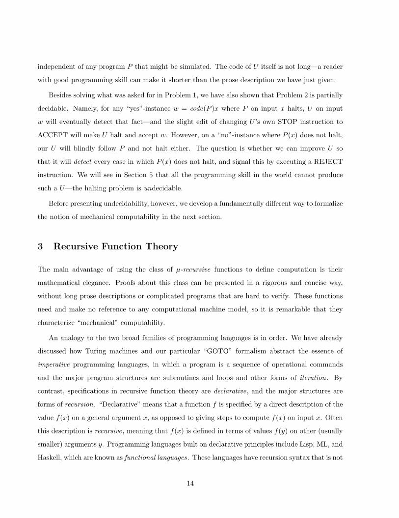
Besides solving what was asked for in Problem 1, we have also shown that Problem 2 is partially
decidable. Namely, for any “yes”-instance w = code(P )x where P on input x halts, U on input
w will eventually detect that fact—and the slight edit of changing U ’s own STOP instruction to
ACCEPT will make U halt and accept w. However, on a “no”-instance where P (x) does not halt,
our U will blindly follow P and not halt either. The question is whether we can improve U so
that it will detect every case in which P (x) does not halt, and signal this by executing a REJECT
instruction. We will see in Section 5 that all the programming skill in the world cannot produce
such a U—the halting problem is undecidable.
Before presenting undecidability, however, we develop a fundamentally different way to formalize
the notion of mechanical computability in the next section.
3 Recursive Function Theory
The main advantage of using the class of µ-recursive functions to define computation is their
mathematical elegance. Proofs about this class can be presented in a rigorous and concise way,
without long prose descriptions or complicated programs that are hard to verify. These functions
need and make no reference to any computational machine model, so it is remarkable that they
characterize “mechanical” computability.
An analogy to the two broad families of programming languages is in order. We have already
discussed how Turing machines and our particular “GOTO” formalism abstract the essence of
imperative programming languages, in which a program is a sequence of operational commands
and the major program structures are subroutines and loops and other forms of iteration. By
contrast, specifications in recursive function theory are declarative, and the major structures are
forms of recursion. “Declarative” means that a function f is specified by a direct description of the
value f(x) on a general argument x, as opposed to giving steps to compute f(x) on input x. Often
this description is recursive, meaning that f(x) is defined in terms of values f(y) on other (usually
smaller) arguments y. Programming languages built on declarative principles include Lisp, ML, and
Haskell, which are known as functional languages. These languages have recursion syntax that is not
14

greatly different from the recursion schemes presented here. They also draw upon Church’s lambda
calculus, which can be called the world’s first general programming language. A formal proof of
equivalence between lambda calculus and the Turing machine model (via a programming language
called I) can be found in [Jones 1997], which presents computability theory from a programming
perspective.1
In this section, we will describe this functional approach to computation and code some simple
functions using recursion. Owing to space limitation, we will not present a complete proof that
the class of µ-recursive functions is the same as the class of (partial) computable functions on a
Turing machine. The full proof can be found in standard texts such as [Sudkamp, 1997]. All the
functions we consider have one or more non-negative integers as arguments, and produce a single
non-negative integer value.
Before presenting formal definitions, we qualify the above ideas with a few examples. Consider
first the simple definition of a two-variable linear function by
h(y, z) = z + 2 ∗ y + 1. (1)
Here h(y, z) is defined with the aid of other functions (here, plus and times) and quantities (here,
2 and 1) that presumably have already been defined or given. This is an example of an explicit
definition because all entities on the right-hand side are known—in particular, this definition does
not involve recursion. If we rewrite the infix functions + and ∗ in prefix-function style as “plus”
and “times,” the expression becomes
h(y, z) = plus(z, plus(times(2, y), 1)), (2)
and we can glimpse another hallmark of functional languages: function names can be regarded as
parameters the same way that variable names can. Now consider the somewhat-similar definition
of a one-variable function by
f(x) = f(x− 1) + 2 ∗ (x− 1) + 1, (3)
1Turing created an addendum to his seminal paper [Turing, 1936] showing that his definition of a (partial) com-
putable function was equivalent to the one proposed by Church. The lambda calculus uses essentially a single
execution scheme called reduction to govern its computations, and by suitable conditioning one can make this scheme
carry out recursion. Another declarative language, Prolog, also fixes a single execution scheme that tries to limit the
operational decisions the programmer needs to make, and also relies upon recursion.
15

together with a base case such as f(0) = 0. Here not every quantity on the right-hand side is
known—one must first know f(x− 1) to compute f(x). However, this is still “declarative” insofar
as f(x) is defined in terms of known quantities and values f(y) for other (smaller) arguments y.
The reader may check that this is a recursive definition of the squaring function.
Why use recursion? One reason is that explicit definition by itself is known not to be powerful
enough to capture the essence of mechanical computation. The next two sections define the two
principal schemes of recursion in recursive function theory.
3.1 Primitive Recursive Functions
The class of primitive recursive functions is built up from the following set of basic functions, which
are the only ones we need to pre-suppose are “known”:
1. The successor function S is defined for all x by S(x) = x+ 1.
2. The zero function Z is defined for all x by Z(x) = 0. The constant 0 is also provided here.
3. For all fixed numbers i and n with 1 ≤ i ≤ n, the projection function pni is defined for all
n-tuples (x1, x2, . . . , xn) by pni (x1, x2, . . . , xn) = xi.
The primitive recursive functions are constructed from the basic functions by applications of
the following two operations. The case n = 0 is allowed in them; a 0-variable function is the same
as a constant, and a 0-tuple is the empty list.
1. Functional composition: Given k-many functions g1, . . . , gk that each take n variables, and a
function h that takes k variables, one can define a function f of n variables by
f(x1, . . . , xn = h(g1(x1, . . . , xn), g2(x1, . . . , xn), . . . , gk(x1, . . . , xn)). (4)
If g1, . . . , gk and h are primitive recursive, then f is defined to be primitive recursive.
2. Primitive recursion: Given a function g that takes n variables, and a function h that takes
n+ 2 variables, one can define a function f of n+ 1 variables by
f(x1, . . . , xn, 0) = g(x1, . . . , xn); (5)
f(x1, . . . , xn, S(y)) = h(x1, . . . , xn, y, f(x1, . . . , xn, y)). (6)
16

If g and h are primitive recursive, then f is defined to be primitive recursive.
Here (5) is the basis and (6) is the recursion step. It is conventional to call x1, . . . , xn the
parameters and y the recursion variable. From a computational viewpoint, the scheme is easy to
interpret. Given integer values for variables x1, . . . , xn and z, how can we evaluate f(x1, . . . , xn, z)?
We start building a table T in which each row y contains the value of f(x1, . . . , xn, y). The basis step
gives us the top row via T [0] = f(x1, . . . , xn, 0) = g(x1, . . . , xn). Whenever we have filled a row y, we
can fill the next row via the recursion step, via T [y+1] = f(x1, . . . , xn, S(y)) = h(x1, . . . , xn, y, T [y]).
As soon as row z is filled, using y such that z = S(y), we are done. The point is that provided g and
h are computable, the function f is also computable. Functional composition likewise preserves
computability. Moreover, since the basic functions are all total and produce non-negative values,
every function that we can build up in this manner is also total and produces non-negative values.
Definition 3.1 A function is said to be primitive recursive if it can be built up from the
successor, zero and projection functions by a finite number of applications of composition and
primitive recursion.
Example 3.1 To show how the scheme of primitive recursion models the informal recursion defin-
ing the function f of one variable (so we have n = 0) in equation (3), take “g()” to be the constant
0, and take h to be the two-variable function h(y, z) = z+2y+1, which happens to be our example
of “explicit definition” in (1). Then we have f(0) = 0 and
f(S(y)) = h(y, f(y)) = f(y) + 2 ∗ y + 1.
With “x− 1” in place of “y” and “x” in place of “S(y),” this is the same as (3). We will return to
this notational difference later.
As the prefix form (2) indicates, h itself can be built up via functional composition from the plus
and times functions. It is interesting to see how the usual functions of arithmetic can themselves
be constructed from the rather Spartan basis we have been given. To begin with, the constants
1, 2, . . . are formally introduced by functional composition, with “g1()” as the constant 0 and “h”
as the successor function, via 1 = S(0), 2 = S(1) = S(S(0)), 3 = S(2), and so on.
17
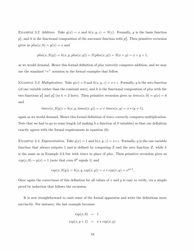
Example 3.2 Addition. Take g(x) = x and h(x, y, z) = S(z). Formally, g is the basis function
p11, and h is the functional composition of the successor function with p3
3. Then primitive recursion
gives us plus(x, 0) = g(x) = x and
plus(x, S(y)) = h(x, y, plus(x, y)) = S(plus(x, y)) = S(x+ y) = x+ y + 1,
as we would demand. Hence this formal definition of plus correctly computes addition, and we may
use the standard “+” notation in the formal examples that follow.
Example 3.3 Multiplication. Take g(x) = 0 and h(x, y, z) = x+z. Formally, g is the zero function
(of one variable rather than the constant zero), and h is the functional composition of plus with the
two functions p31 and p3
3 (so k = 2 here). Then primitive recursion gives us times(x, 0) = g(x) = 0
and
times(x, S(y)) = h(x, y, times(x, y)) = x+ times(x, y) = x ∗ (y + 1),
again as we would demand. Hence this formal definition of times correctly computes multiplication.
Note that we had to go to some length (of making h a function of 3 variables) so that our definition
exactly agrees with the formal requirements in equation (6).
Example 3.4 Exponentiation. Take g(x) = 1 and h(x, y, z) = x∗z. Formally, g is the one-variable
function that always outputs 1 and is defined by composing S and the zero function Z, while h
is the same as in Example 3.3 but with times in place of plus. Then primitive recursion gives us
exp(x, 0) = g(x) = 1 (note that even 00 equals 1) and
exp(x, S(y)) = h(x, y, exp(x, y)) = x ∗ exp(x, y) = xy+1.
Once again the correctness of this definition for all values of x and y is easy to verify, via a simple
proof by induction that follows the recursion.
It is now straightforward to omit some of the formal apparatus and write the definitions more
succinctly. For instance, the last example becomes
exp(x, 0) = 1
exp(x, y + 1) = x ∗ exp(x, y).
18

This resembles a program one would actually write, especially in a language like C that does not
provide exponentiation as a built-in operator.
At this point the alert reader, noting the way our schemes all involve non-negative numbers,
will first wonder how on earth we can ever define subtraction this way. The key is that the syntax of
primitive recursion allows us to define a function P (y) that computes “proper subtraction by 1,” and
then use P to define proper subtraction itself. The word “proper” here means that any negative
value is replaced by 0, in order to maintain our restriction to the non-negative numbers. The
definitions are
P (0) = 0
P (S(y)) = y
sub(x, 0) = x
sub(x, S(y)) = P (sub(x, y))
For P we took h(y, z) = y, i.e. h = p21, and for sub we took h(y, z) = P (z). To trace this out,
sub(3, 2) = P (sub(3, 1)) = P (P (sub(3, 0)) = P (P (3)) = P (2) = 1, and sub(2, 3) = P (P (P (2))) =
P (0) = 0, which is the “proper” value.
Second, the reader may have felt uncomfortable defining functions in terms of “S(y)” rather
than “y.” For example, the primitive recursion for the factorial function, with 0! standardly defined
to be 1, gives us
fact(0) = 1 | fact(y+1) = (y+1)*fact(y);
here “|” separates the base and recursion cases. This would actually be valid syntax in the pro-
gramming language ML except that “fact(y+1)” is an illegal function header. The syntax of ML
forces one to write it this way:
fact(0) = 1 | fact(y) = y*fact(y-1);
this is literally the example used in many texts. To make the formal equation (6) for primitive
recursion reflect the syntax of programming languages, we can use P in place of S to change it to
f(x1, . . . , xn, y) = h(x1, . . . , xn, y, f(x1, . . . , xn, P (y))), (7)
19

or alternately make the middle argument of h be P (y) instead of y. Either way, one might expect
to be able to recover the function S by defining it in terms of P and the other two basis functions,
just as we defined P in terms of S above. However, this is impossible—one could never define any
increasing functions at all. This curious asymmetry partly explains why primitive recursion was
defined the way it is. Nevertheless, if S as well as P is provided in the basis, then one can use the
modified definition and obtain exactly the same class of primitive recursive functions. For instance,
addition is definable by plus(x, 0) = x | plus(x, y) = S(plus(x, P (y))), and so on. Hence primitive
recursion is for the most part exactly what ML and other functional languages do.2
Finally, the reader may wonder what has become of functions defined on strings. A string over
an alphabet Σ can always be identified with its number in the standard lexicographic enumeration of
Σ∗, with ε corresponding to 0. Then a string function f : Σ∗ → Σ∗ can be called primitive recursive
if the corresponding numerical function (of one variable) is primitive recursive. For instance, the
function that appends a ‘1’ to a binary string x corresponds to 2x + 2. Cutting the other way,
under some transparent encoding of negative and rational and complex numbers (etc.) by strings,
one can extend the concept of primitive recursion to define addition and multiplication and nearly
all familiar mathematical functions in their full generality. The meaning and proof of the following
statement should now be clear; full detail can be found in [Sudkamp, 1997].
Theorem 3.1 Every primitive recursive function is computable by a Turing machine.
The converse is false, however. A famous example of a computable total function that
is not primitive recursive is Ackermann’s function; this and other examples may be found in
[McNaughton, 1993]. To obtain all computable functions we need to introduce one more scheme
of recursion—at the inevitable cost, however, of opening a Pandora’s box of functions that are no
longer total.
2Primitive recursion has its counterpart in imperative languages as well, aside from the fact that most of them
support recursion directly. The “table T [y]” computation above shows how primitive recursion can be simulated by
a simple for-loop for y = 0 to z do. . . end that fixes its bounds and never alters y in the loop body. A theorem
[Meyer and Ritchie] in programming languages states that the primitive recursive functions are exactly the total
functions computable by programs that use only if-then-else and nested for-loops.
20
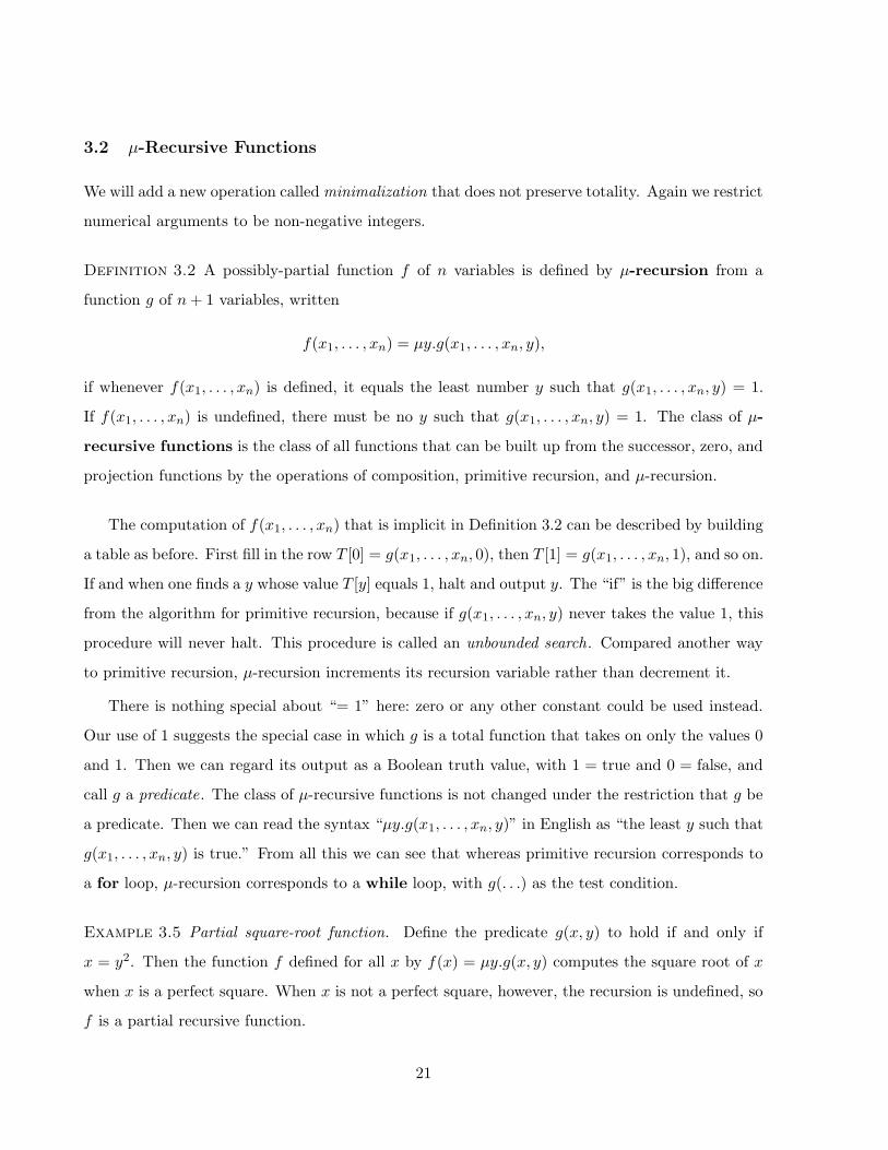
3.2 µ-Recursive Functions
We will add a new operation calledminimalization that does not preserve totality. Again we restrict
numerical arguments to be non-negative integers.
Definition 3.2 A possibly-partial function f of n variables is defined by µ-recursion from a
function g of n+ 1 variables, written
f(x1, . . . , xn) = µy.g(x1, . . . , xn, y),
if whenever f(x1, . . . , xn) is defined, it equals the least number y such that g(x1, . . . , xn, y) = 1.
If f(x1, . . . , xn) is undefined, there must be no y such that g(x1, . . . , xn, y) = 1. The class of µ-
recursive functions is the class of all functions that can be built up from the successor, zero, and
projection functions by the operations of composition, primitive recursion, and µ-recursion.
The computation of f(x1, . . . , xn) that is implicit in Definition 3.2 can be described by building
a table as before. First fill in the row T [0] = g(x1, . . . , xn, 0), then T [1] = g(x1, . . . , xn, 1), and so on.
If and when one finds a y whose value T [y] equals 1, halt and output y. The “if” is the big difference
from the algorithm for primitive recursion, because if g(x1, . . . , xn, y) never takes the value 1, this
procedure will never halt. This procedure is called an unbounded search. Compared another way
to primitive recursion, µ-recursion increments its recursion variable rather than decrement it.
There is nothing special about “= 1” here: zero or any other constant could be used instead.
Our use of 1 suggests the special case in which g is a total function that takes on only the values 0
and 1. Then we can regard its output as a Boolean truth value, with 1 = true and 0 = false, and
call g a predicate. The class of µ-recursive functions is not changed under the restriction that g be
a predicate. Then we can read the syntax “µy.g(x1, . . . , xn, y)” in English as “the least y such that
g(x1, . . . , xn, y) is true.” From all this we can see that whereas primitive recursion corresponds to
a for loop, µ-recursion corresponds to a while loop, with g(. . .) as the test condition.
Example 3.5 Partial square-root function. Define the predicate g(x, y) to hold if and only if
x = y2. Then the function f defined for all x by f(x) = µy.g(x, y) computes the square root of x
when x is a perfect square. When x is not a perfect square, however, the recursion is undefined, so
f is a partial recursive function.
21

Example 3.6 Linear programming. The standard simplex algorithm uses a while loop that ex-
ecutes a basic pivot step until a predicate expressing optimality holds. Hence the function that
embodies the solution to a linear programming problem is µ-recursive. In point of fact, because a
bound on the number of polytope corner points is explicitly definable from the problem instance,
the same function can be computed via a simple for loop, so it is primitive recursive. However, the
former method is usually much faster.
Part (a) of the next theorem expresses the fact that while loops, together with if-then-else,
suffice to make a general-purpose programming language. Part (b) is the gist of the famous theorem,
credited in various forms to various sources, that at most one while loop is needed in any program.
Theorem 3.2 (a) A (partial) function is µ-recursive if and only if it is a Turing-computable
(partial) function.
(b) Moreover, given any Turing machine T , we can find a primitive recursive function u and a
primitive recursive predicate t such that for all x, T (x) = u(µy.t(x, y)).
In the standard proof of part (b), the predicate t(x, y) is designed to hold if and only if y encodes
the sequence of configurations of a halting computation of T on input x, and the function u picks
off the output from the final configuration. To complete the proof of (a), all one needs to show is
that given a Turing machine that computes g in Definition 3.2, one can build a Turing machine
that computes f . This is done by following the unbounded-search procedure sketched above.
The corresponding theorem for formal languages also merits mention here. In Chapter 30 we
defined the characteristic function of a language L to be the function fL defined for all x by
fL(x) = 1 if x ∈ L, fL(x) = 0 if x /∈ L. This is simply the predicate corresponding to membership
in L. The partial characteristic function still takes the value 1 when x ∈ L, but is undefined when
x /∈ L.
Theorem 3.3 (a) A language is recursive if and only if its characteristic function is µ-recursive.
(b) A language is r.e. if and only if its partial characteristic function is µ-recursive.
Part (a) explains how the term “recursive” became applied to languages and predicates as a syn-
onym for “decidable.” It is important to recall that not all languages L accepted by Turing machines
22

have computable characteristic functions (i.e., are decidable); unless we find a Turing machine ac-
cepting L that halts for all inputs, all we know is that the partial characteristic function of L is
(partial-) computable. Before proceeding to undecidable languages, we take time to interpret these
two theorems and others presented in the two previous chapters.
4 Equivalence of Computational Models and the Church-Turing
Thesis
In Chapter 30 we introduced various machine models, the most important of which is the Turing
machine. In Chapter 31 we introduced the grammar hierarchy of Chomsky, of which the most
powerful was the Type-0 grammar. Here we have presented the purely mathematical model of
µ-recursive functions. Although these models were defined over different domains for different
purposes, they are all equivalent in a precise technical sense—they all define the same class of
computable functions and decidable languages, and the same class of partial computable functions
and partially decidable languages.
We can summarize all this by saying that Turing machines, type-0 grammars, and µ-recursive
functions have the same problem-solving power.
This equivalence extends to vastly many other computational models, of which we mention a
few:
(1) Cellular Automata. Cellular automata are intended to model the evolution of a colony of
micro-organisms. Each cell is a deterministic finite automaton that receives its input in dis-
crete time steps from neighboring cells, so that its current state is defined by its own previous
state and the previous states of its neighbors. All the cells execute the same DFA. There are
different schemes for specifying the representation of the input to a cellular automaton and
its output. But under any reasonable scheme, the largest class of problems that can be solved
on cellular automata coincides with the class of solvable problems on a Turing machine.
(2) String-Rewriting Systems A string-rewriting system is similar to a grammar. The main dif-
ference is that there are no non-terminals. Let the input alphabet be Σ. The production
rules of a rewriting system T will be of the form α → β where α and β are strings over Σ.
23

One can apply such a rule by replacing any occurrence of α in a string by β. T is defined as
a finite set of rewrite rules, along with a finite set of initial strings. The language generated
by T is defined as the set of strings that can be obtained from an initial string by applying
the rewrite rules a finite number of times. The systems proposed before 1930 by Thue and
Post fall roughly into this category. It turns out that the class of string-rewriting languages
is the same as the r.e. languages (see [Book, 1993]).
(3) Tree-Rewriting Systems. These are similar to string-rewriting systems except that the local
edits are done on subtrees of a tree, and rules may have more than one argument. The subtrees
typically represent terms in algebraic or logical expressions that are being operated on. Under
reasonable schemes for encoding numbers or strings by trees, all known tree-rewriting systems
generate r.e. languages or compute partial recursive functions. Church’s λ-calculus and most
formal systems of logic fall into this category.
(4) Extensions of Turing’s Model. As mentioned in Chapter 30, one can also create numerous
modifications to the basic Turing machine model, such as having multi-dimensional tapes or
binary trees with MOVE UP, MOVE DOWN LEFT, and MOVE DOWN RIGHT instructions
(the latter are tantamount to having random-access to stored values), allowing nondetermin-
ism or alternation, making computation probabilistic (see Chapter 35, Section 2), and so on.
All of these machines compute the same functions as the simple one-tape Turing machine.
(5) Random-Access Machines and High-Level Programming Languages. These can be mentioned
in tandem because a RAM, as described in Chapter 30, is just an idealization of assembly or
machine language. Every high-level language yet devised can be compiled into some machine
language. Even the standard Java Virtual Machine is little more than a RAM, with some
added handling of class objects via pointers that is not unlike the workings of a pointer
machine, and some hooks to enable the host system to control physical devices and network
communications. Without excessive effort one can extend the construction of a universal
Turing machine in Section 2 to handle the case where P is a RAM program rather than a
GOTO program. The registers of P can be simulated on the tape by adding one more tape
symbol # and using strings of the form #i#j#, where i is the register’s number and j is its
contents. As stated in Chapter 30, Section 4, this simulation is even fairly efficient. Hence all
24

these high-level languages have the same problem-solving power as the lowly one-tape Turing
machine.
The convergence of so many disparate formal models on the same class of languages or functions
is the main evidence for the assertion that they all exactly capture the informal notion of what
is mechanically or humanly computable. This assertion is called the Church-Turing thesis. In
one form, it asserts that every problem that is humanly solvable is solvable by a Turing machine.
Put more precisely, any cognitive process that a human being could or will ever use to distinguish
certain numbers or strings as “good” defines an r.e. language—and if it also would determine that
any other given number or string is “bad,” it defines a recursive language. An extension of the thesis
claims that no one will ever design a physical device to compute functions that are not µ-recursive.
The Church-Turing thesis is not a mathematical conjecture and is not subject to mathematical
proof; it is not even clear whether the extension is resolvable scientifically.
5 Undecidability
The Church-Turing thesis implies that if a language is undecidable in the formal sense defined
above, then the problem it represents is really, humanly, physically undecidable. The existence of
languages that are not even partially decidable can be established by a counting argument: Turing
machines can be counted 1, 2, 3, . . ., but Cantor proved that the totality of all sets of integers
cannot be so counted. Hence there are sets left over that are not accepted, let alone decided, by
any program. This argument, however, does not apply to languages or problems that one can state,
since these are also countable. The remarkable fact is that many easily-stated problems of high
practical relevance are undecidable. This section shows that the five remaining problems on our
list in Section 2.1, namely 2–5 and 7, are all unsolvable.
5.1 Diagonalization and Self-reference
Undecidability is inextricably tied to the concept of self-reference, and so we begin by looking
at this perplexing and sometimes paradoxical concept. The simplest examples of self-referential
paradox are statements such as “This statement is false” and “Right now I am lying.” If the
25
former statement is true, then by what it says, it is false; and if false, it is true. . . The idea and
effects of self-reference go back to antiquity; a version of the latter “liar” paradox ascribed to the
Cretan poet Epimenides even found its way into the New Testament, Titus 1:12–13. For a more-
colorful example, picture a barber of Seville hanging out an advertisement reading, “I shave those
who do not shave themselves.” When the statement is applied to the barber himself, we need to
ask: Does he shave himself? If yes, then he is one of those who do shave themselves, which are
not the people his statement says he shaves. The contrary answer no is equally untenable. Hence
the statement can be neither true nor false (it may be good ad copy), and this is the essence of
the paradox. Such paradoxes have made entry into modern mathematics in various forms. We
will present some more examples in the next few paragraphs. Many variations on the theme of
self-reference can be found in the books of the logician and puzzlist Raymond Smullyan, including
[Smullyan, 1978] and [Smullyan, 1992].
Berry’s paradox concerns English descriptions of natural numbers. For example, the number
24 can be described by many different phrases: “twenty-four,” “six times four,” “four factorial,”
etc. We are interested in the shortest of such descriptions, namely one(s) having the fewest letters.
Here, “two dozen” beats all of the above. Clearly there are (infinitely) many positive integers whose
shortest descriptions require one hundred letters or more. (A simple counting argument can be used
to show this. The set of positive integers is infinite, but the set of positive integers with English
descriptions of fewer than one hundred letters is finite.) Let D denote the set of positive integers
that do not have English descriptions of fewer than one hundred letters. Thus D is not empty.
It is a well-known fact in set theory that any nonempty subset of positive integers has a smallest
integer. Let x be the smallest integer in D. Does x have an English description of fewer than one
hundred letters? By the definition of the set D and x, the answer is yes: such a description of x
is, “the smallest positive integer that cannot be described in English in fewer than one hundred
letters.” This is an absurdity because the quoted part of the last sentence is clearly a description
of x, and it contains fewer than one hundred letters.
Russell’s paradox similarly turns on issues in defining sets. In formal mathematics, we can
perfectly easily describe “the set of all sets that do not include themselves as elements” by the
definition S = {x|x /∈ x}. The question “Is S ∈ S?” leads to a real conundrum. This also resembles
the barber paradox, with “/∈” read as “does not shave.” This paradox forced the realization that
26

the formal notion of a set , and importantly the formal rules that apply to sets, do not and cannot
apply to everything that we informally regard as being a “set.”
Our last example is a charming paradox named for the mathematician William Zwicker. Con-
sider the collection of all two-person games that are normal in the sense that every play of the game
must end after a finite number of moves. Tic-tac-toe is normal since it always ends within nine
moves, while chess is normal because the official “fifty move rule” prevents games from going on
forever. Now here is hypergame. In the first move of hypergame, the first player calls out a normal
game—and then the two players go on to play that game, with the second player making the first
move. Now we need to ask, “Is hypergame normal?” If yes, then it is legal for the first player to
call out “hypergame!”—since it is a normal game. By the rules, the second player must then play
the first move of hypergame—and this move can be calling out “hypergame!” Thus the players can
keep saying “hypergame” without end, but this contradicts the definition of a normal game. On
the other hand, suppose hypergame is not normal. Then in the first move, player 1 cannot call out
hypergame and must call a normal game instead—so that the infinite move sequence given above
is not possible and hypergame is normal after all!
Let us try to implement Zwicker’s paradox. To play hypergame, we need a way of formalizing
and encoding the rules of a game as a string x, and we need a decision procedure isNormal(x)
to tell if the game is normal. Then the rules of hypergame are easily formalized: pick a string x,
verify isNormal(x), and play game x. Let h be the string encoding of these rules. Now we get a
real contradiction when isNormal(h) is run. We must conclude that either (i) our formalization
of games is inadequate or inconsistent, or (ii) a decision procedure isNormal simply cannot exist.
Now (i) is the way out for Russell’s paradox with “sets” in place of “games.” For computation,
however, we know that our formalization is adequate and consistent—and hence we will be faced
with conclusion (ii), namely that our corresponding computational problems are unsolvable.
Before showing how the above paradoxes can be modified and ingrained into our problems, we
need to review the 0-1 encoding of GOTO programs from Section 2.2, including the conventions
that ACCEPT has the same code 100 as STOP for programs that accept languages, and that such
an ACCEPT statement be last and unique. We may assign the code 101 to REJECT, which may
appear anywhere. If a binary string x encodes a program P , it is easy to decode x into P , and we
may identify x with P . If x does not encode a legal GOTO program, this fact is easy to detect.
27

Then we may choose to treat x as an alternate code for the trivial GOTO program that consists
of a single REJECT statement.
Now we can define the so-called “diagonal language” Ld as follows:
Ld = {x | x is a GOTO program that does not accept the string x} (8)
This language consists of all programs in GOTO language that do not halt in the ACCEPT state-
ment when given their own encoding as input—they may either REJECT or not halt at all on
that input. For example, consider x = 01111101101100, which encodes a program that accepts
any string beginning with 1 and rejects any string beginning with 0. Then x ∈ Ld since the pro-
gram does not accept 01111101101100. Note the self-reference in (8). Although the definition of
Ld seems artificial, its importance will become clear in the next section when we use it to show
the undecidability of other problems. First we prove that Ld is not even accepted by any Turing
machine, let alone decided by one.
Theorem 5.1 Ld is not recursively enumerable.
Proof. Suppose for the sake of contradiction that Ld is r.e. Then there is a GOTO program
that accepts Ld—call it P . Now what does P do on input x = code(P )? If P accepts x, then x is
not in Ld, but this contradicts L(P ) = Ld. But if P does not accept x, then x is in Ld, and this
also contradicts L(P ) = Ld. Hence a program P such that L(P ) = Ld cannot exist, and so Ld is
not r.e.
The definition of Ld is motivated by Russell’s paradox, reading “/∈” as “does not accept.”
Whereas in Russell’s paradox we had to conclude that S is not a set , here we conclude that Ld is
not a Turing-acceptable set.
We can similarly carry over Zwicker’s paradox by treating a given string x as formally defining
“Game-x” as follows: The first player decodes x into a GOTO program P , and then tries to choose
some string x′ in the language L(P ). If L(P ) is empty, in particular if x decodes to the trivial
program “1. REJECT” as stipulated above, then the game ends then and there. But if the first
player finds such an x′, then the second player must play the same way with x′. Then we can
say that x is normal if every play of Game-x must terminate (by reaching a GOTO program that
accepts the empty language) in a finite number of steps. Finally define LZ to be the set of normal
28

strings. By applying the reasoning from Zwicker’s paradox, one can imitate the above proof to
show that LZ is not recursively enumerable.
5.2 Reductions and More Undecidable Problems
Recall from Chapter 30 (section 2.3) the notion of Turing reducibility. Basically, a language L1
is Turing reducible to L2 if there is a halting Turing machine for language L1 using an oracle for
language L2. If L1 is reducible to L2 and L2 is decidable, then so is L1. Basically, one can replace
queries to oracles by executing a halting computation for L2. The contrapositive of this statement
can be used to show undecidability. If L1 is undecidable, then so is L2. We will first express
Problem (2) as a language:
LU = {code(P )111x| P accepts the string x}.
Thus LU takes as input a program in GOTO, and a binary string x, and accepts the encoded pair
(P, x) if and only if P accepts x. (Note 111 is used as a separator between P and x.) The universal
program presented in Section 2.2 accepts the language LU hence it is recursively enumerable. We
will show that LU is not recursive. First, we will show a simple fact about recursive languages.
Theorem 5.2 Recursive languages are closed under complement.
Proof. Let P be a GOTO program for language L. The program P ′ obtained by exchanging
ACCEPT and REJECT instructions is easily seen to accept the language L. This standard trick
works to complement the computations of most of the deterministic devices (such as DFA). •
Now we show that LU is not recursive.
Theorem 5.3 LU is not recursive.
Proof. Consider the language L′U = {x| x when interpreted as a GOTO program accepts its
own encoding}. Obviously, L′U = LD. Since LD is not recursively enumerable, it is not recursive.
(Recall that the set of recursive languages is a subset of recursively enumerable languages.) By the
above theorem, L′U is not recursive. Finally, note that LU can be reduced to L′
U as follows: Given
an algorithm for LU , we can construct an algorithm for L′U as follows: Let P be an algorithm for
LU . To construct an algorithm for L′U simply note the connection between the two problems. An
29

input string x belongs to L′U if and only if x111x belongs to LU . Thus, a simple copy program
(similar to one presented in Section 2) can be first used to convert the input x into x111x. Move the
scanning head back to the leftmost character of the first copy of x. Now simply run the program P .
Note that the program P ′ described above is being constructed using only P , not x. This reduction
shows that LU is not recursive.
Next we consider problem (6) in our list. Earlier we showed that a special case of this problem
(when the input is restricted to type-1 grammar) is totally solvable. It is not hard to see that
the general problem is partially solvable. (To see this, suppose there is a derivation for a string x
starting from S, the start symbol of the grammar. Suppose the length of one such derivation is k.
A program can try all possible derivations of length 1, 2, etc. until it succeeds. Such a program
will always halt on strings x generated by the grammar G. Thus the language
{< G > #x| < G > is a type-0 grammar and x can be generated by G }
is recursively enumerable. A standard result from
formal language theory [Hopcroft and Ullman, 1979] is that for every Turing machine M , there
is a type-0 grammar such that L(M) = T (G). This conversion is the reduction that shows that the
language stated above is not recursive.
By a more elaborate reduction (from LD), it can be shown that tiling problem (4) in our
list is also not partially decidable. We will not do it here and refer the interested reader to
[Harel, 1992]. But we would like to point out how the undecidability result can be used to infer
a result about aperiodic tilings. This deduction is interesting because the result appears to have
some deep implications and is hard to deduce directly. We need the following definition before we
can state the result. A different way to pose the tiling problem is whether a given set of tiles can
tile an entire plane in such a way that all the adjacent tiles have the same color on the meeting
quarter. (Note that this question is different from the way we originally posed it: Can a given set
of tiles tile any finite rectangular region? Interstingly, the two problems are identical in the sense
that the answer to one version is “yes” if and only if it is “yes” for the other version.) Call a tiling
of the plane it periodic if one can identify a k × k square such that the the entire tiling is made
by repeating this k × k square tile. Otherwise, call it aperiodic. Consider the question: Is there
a (finite) set of unit tiles which can tile the plane, but only aperiodically? The answer is “yes”
and it can be shown by from the total undecidability of tiling problem. Suppose the answer is
30

“no”. Then, for any given set of tiles, the entire plane can be tiled if and only if the plane can be
tiled periodically. But a periodic tiling can be found, if one exists, by trying to tile a k × k region
for successively increasing values of k. This process will eventually succeed (in a finite number of
steps) if the tiling exists. This will make the tiling problem partially decidable, which contradicts
the total undecidability of the problem. This means that the assumption that the entire plane can
be tiled if and only if some k×k region can be tiled is wrong. Thus there exist a (finite) set of tiles
that can tile the entire plane, but only aperiodically.
We conclude with a brief remark about problem (7) in our list. After many years of effort
by several mathematicians and computer scientists (including Davis and Robinson), Matiyasevich
found an effective way to transform a given Turing machine T into a set of equations in variables
x, y1, . . . , ym such that for any x, T on input x halts if and only if the other m variables can be set
to solve the equations. This reduction shows that Hilbert’s tenth problem is undecidable. Details
behind this reduction can be found in [Floyd and Beigel, 1994].
6 Defining Terms
Decision Problem: A computational problem with yes/no answer. Equivalently a function whose
range consists of two values {0, 1}.
Decidable Problem: A decision problem which can be solved by a GOTO program that halts on
all inputs in a finite number of steps. For emphasis, the equivalent term totally decidable problem
is used. The associated language is called recursive.
Partially Decidable Problem: A decision problem that can be solved by a GOTO program
which halts (and outputs ACCEPT) on all yes instances. The program may or may not halt on
no instances. Equivalently, the collection of yes instance strings forms a type-0 language. (See
Chapter 31.)
Recursively Enumerable Language: Same as partially decidable language. This term was not
used in this chapter.
µ-Recursive Function: A function that is a basic function (Zero, Successor or Projection), or
one that can be obtained from other µ-recursive functions using composition and µ-recursion.
31

Recursive Language: A language that can be accepted by a GOTO program that halts on all
inputs. The associated problem is called decidable.
Solvable Problem: A computational problem which can be solved by a halting GOTO program.
The problem may have a non-binary output.
Totally Undecidable Problem: A problem which cannot be solved by a GOTO program. Equiv-
alently, the set of yes instance strings is not a type-0 language.
Undecidable Problem: A decision problem that is not (totally) decidable. It could be partially
decidable or totally undecidable.
Universal Turing Machine: A Turing machine that can simulate any other Turing machine.
Unsolvable Problem: A computational problem which is not solvable. The associated function
will be called uncomputable function.
References
[Book, 1993] Book, R. and Otto, F. 1993 String Rewriting Systems. Springer-Verlag, Berlin.
[Chomsky, 1956] Chomsky, N. 1956. Three models for the description of language. IRE Trans. onInformation Theory. 2(2):113-124.
[Chomsky, 1963] Chomsky, N. 1963. Formal properties of grammars. In Handbook of Math. Psych.Vol. 2, 323-418. John Wiley and Sons, New York.
[Davis, 1958] Davis, M. 1958. Computability and Unsolvability McGraw-Hill, New York.
[Davis, 1980] Davis, M. 1980. What is computation? in Mathematics Today-Twelve Informal Es-says. L. Steen (ed.) 241-259.
[Floyd and Beigel, 1994] Floyd, R.W. and Beigel, R. 1994 The Language of Machines: an Intro-duction to Computability and Formal Languages. Computer Science Press, New York.
[Gurari, 1989] Gurari, E. 1989. An Introduction to the Theory of Computation. Computer SciencePress, Rockville, MD.
[Harel, 1992] Harel, D. 1992. Algorithmics: The spirit of Computing. Addison-Wesley, Reading,MA.
[Harrison, 1978] Harrison, M. 1978. Introduction to Formal Language Theory. Addison-Wesley,Reading, MA.
[Hartmanis, 1994] Hartmanis, J. 1994. On computational complexity and the nature of computerscience. CACM. 37(10):37-43.
[Hartmanis and Stearns, 1965] Hartmanis, J. and Stearns, R. 1965. On the computational com-plexity of algorithms. Trans. Amer. Math. Soc.. 117:285-306.
32

[Hopcroft and Ullman, 1979] Hopcroft, J. and Ullman, J. 1979. Introduction to Automata Theory,Languages and Computation. Addison-Wesley, Reading, MA.
[Jones 1997] Jones, N.D. 1997. Computability and Complexity - From Programming Perspective.MIT Press, Cambridge, MA.
[Kleene, 1956] Kleene, S. 1956. Representation of events in nerve nets and finite automata. InAutomata Studies, 3-41. Princeton University Press, NJ.
[Kohavi, 1978] Kohavi, Z. 1978. Switching and Finite Automata Theory. McGraw-Hill.
[Kolmogorov and Uspenskii, 1958] Kolmogorov, A. and Uspenskii, V. 1958. On the definition of analgorithm. Uspekhi Mat. Nauk. 13:3-28.
[Li and Vitanyi, 1993] Li, M. and Vitanyi, P. 1993. An Introduction to Kolmogorov Complexity andIts Applications. Springer-Verlag.
[Meyer and Ritchie] Meyer, A. and Ritchie, D. 1967 The complexity of LOOP programs. Proc.22nd ACM National Conf., 465-469.
[McNaughton, 1993] McNaughton, R. 1993 Elementary Computability, Formal Languages and Au-tomata. ZB Publishing Industries, Lawrence, Kansas.
[Minsky, 1967] Minsky, M. 1967 Computation: Finite and Infinite Machines Prentice Hall, Engle-wood Cliffs, NJ.
[Post, 1943] Post, E. 1943. Formal reductions of the general combinatorial decision problems. Amer.J. Math. 65:197-215.
[Robinson, 1991] Minsky’s small universal Turing machine. International Journal of Mathematics.2(5):551-562.
[Rogers, 1967] Rogers, H. 1967 Theory of Recursive Functions and Effective Computability. MITPress, Cambridge, MA.
[Sipser, 1996] Sipser, M. 1996 Introduction to the Theory of Computation, First Edition, 1996.PWS Publishing Company, Boston, MA.
[Smullyan, 1978] Smullyan, R. 1978What is the Name of this Book?, Prentice-Hall, Inc., EnglewoodCliffs, NJ.
[Smullyan, 1992] Smullyan, R. 1992 Satan, Cantor and Infinity, Alfred A. Knopf Inc., 1992.
[Sudkamp, 1997] Sudkamp, T. 1997. Languages and Machines An Introduction to the Theory ofComputer Science, Addison-Wesley Longman Inc.
[Turing, 1936] Turing, A. 1936. On computable numbers with an application to the Entschei-dungsproblem. Proc. London Math. Soc., series 2, 42:230-265, 1936.
[Wood, 1987] Wood, D. 1987. Theory of Computation. Harper and Row.
[Wang, 1961] Wang, H. 1961 Proving theorems by pattern recognition. Bell System Technical Jour-nal, 40:1-42, 1961.
33

Further Information
The fundamentals of computability can be found in many books including the classical
books [Rogers, 1967, Davis, 1958, Minsky, 1967]. More recent books on automata and formal
languages have also devoted at least a few chapters on computability [Floyd and Beigel, 1994,
Gurari, 1989, Harel, 1992, Harrison, 1978, Hopcroft and Ullman, 1979, Sipser, 1996, Wood, 1987].
Early work on computability was motivated by a quest to address profound questions about the
basis of logical reasoning, mathematical proofs and automatic computation. Various formalisms
discussed in this chapter were proposed at around the same time, and soon thereafter, their equiv-
alence was tested. Thus, in a short time, Church thesis took deep roots. Subsequent work has
focussed on resolution of specific problems (as to decidable or not). Two such famous problems
were Hilbert’s tenth problem and word problem for groups. Both problems were eventually shown
to be unsolvable. Another direction of research has been to make finer distinction among unsolvable
problems by introducing degrees of unsolvability. Recursive function theory and lambda calculus
also led to the development of functional programming languages (such as Lisp, Scheme, Haskell,
ML etc.) Computability theory is also closely related to logic, formal deductive systems and struc-
tural complexity. Logic and deductive systems are of interest to philosophers and researchers in
artificial intelligence, as well as computation theorists. Although there are no journals devoted
exclusively to computability, many theory journals (e.g. listed at the end of the last two chapters)
publish papers on this topic. In addition, Annals of Pure and Applied Logic publishes papers on
logic and computability.
34
Related Documents


![IEEE TRANSACTIONS ON MOBILE COMPUTING, …mingli/papers/m3c2.pdf · information [8]–[10] in the coverage area. Besides, instead of delivering all data traffic in one hop like that](https://static.cupdf.com/doc/110x72/5b889eb97f8b9abe1e8bb153/ieee-transactions-on-mobile-computing-minglipapersm3c2pdf-information-810.jpg)


![arXiv:1911.11502v1 [cs.CV] 26 Nov 2019 · Hearing Lips: Improving Lip Reading by Distilling Speech Recognizers Ya Zhao,1 Rui Xu,1 Xinchao Wang,2 Peng Hou,3 Haihong Tang,3 Mingli Song1](https://static.cupdf.com/doc/110x72/6014a8c2cec4c025af3225a0/arxiv191111502v1-cscv-26-nov-2019-hearing-lips-improving-lip-reading-by-distilling.jpg)