Compressive Sensing-Based Sparsity Adaptive Channel ...

applied sciences

Article

Compressive Sensing-Based Sparsity AdaptiveChannel Estimation for 5G Massive MIMO Systems

Imran Khan 1 ID , Madhusudan Singh 2,* and Dhananjay Singh 3,* ID

1 Department of Electrical Engineering, University of Engineering & Technology,Peshawar 814, KPK, Pakistan; [email protected]

2 Endicott College of International Studies, Woosong University, Daejeon 300718, Korea3 Department of Electronics Engineering, Hankuk University of Foreign Studies, Yongin 17035, Korea* Correspondence: [email protected] (M.S.); [email protected] (D.S.); Tel.: +82-105-844-9415 (D.S.)

Received: 30 March 2018; Accepted: 7 May 2018; Published: 9 May 2018�����������������

Abstract: Aiming at a massive multi-input multi-output (MIMO) system with unknown channelpath number, a sparse adaptive compressed sensing channel estimation algorithm is proposed,which is the block sparsity adaptive matching pursuit (BSAMP) algorithm. Based on the joint sparsityof subchannels in massive MIMO systems, the initial set of support elements can be quickly andselectively selected by setting the threshold and finding the maximum backward difference position.At the same time, the energy dispersal caused by the non-orthogonality of the observation matrixis considered, and the estimation performance of the algorithm is improved. The regularization ofthe elements secondary screening is deployed, in order to improve the stability of the algorithm.Simulation results show that the proposed algorithm can quickly and accurately recover massiveMIMO channel state information with unknown channel sparsity and high computational efficiencycompared with other algorithms.

Keywords: 5G; massive MIMO; compressive sensing; sparsity adaptive; a channel estimation

1. Introduction

Massive MIMO (multiple-input multiple-output) technology is one of the key technologies ofnext-generation mobile cellular networks, which can form a massive antenna array by providing alarge number of antennas at the cell base station. It will greatly improve the channel capacity andspectrum utilization and has become a hotspot in the field of wireless communications in recentyears [1]. In a massive MIMO system, a precise channel state information (CSI) is critical, which isdirectly related to the system signal detection, beamforming, resource allocation and so on. The numberof base station antennas in massive MIMO systems has reached hundreds of thousands, which greatlydeepens the complexity of system data processing. Therefore, in order to make full use of the potentialadvantages of massive MIMO technology, the more efficient and low complexity channel estimationalgorithms are worthy of further study. Massive MIMO has various merits over the conventionalMIMO. First, it uses a large number of antennas at the BS due to which the simplest coherent-combinerand linear-precoder can be used for signal processing such MF or ZF. Second, increasing the numberof antennas increases the system capacity substantially using the channel-reciprocity features andwithout increasing feedback-overhead. Third, the reduced power benefits in the uplink/downlink(UL/DL) provide the feasibility to shrink the cell-size, which can be used in micro and pico-cells.

The massive multi-input multi-output (MIMO) system has doubled the capacity of thecommunication system without increasing the signal bandwidth and signal transmission powerand is regarded as the core technology of 5G wireless communication. Channel estimation is the key

Appl. Sci. 2018, 8, 754; doi:10.3390/app8050754 www.mdpi.com/journal/applsci

Appl. Sci. 2018, 8, 754 2 of 13

technology in the physical layer of massive MIMO systems. Its accuracy directly affects the systemperformance under fading channels.

In massive MIMO systems, accurate Channel State Information (CSI) is required to utilize the fullpotential of MIMO systems [2,3]. However, such accurate CSI is not available in real communicationenvironment [4]. With the increasing number of antennas, the receiver has to estimate more channelcoefficients, which effectively increases the pilot overhead, computational complexity and reducesthe overall throughput of the system [5]. This is a challenging issue which has been addressedin [3–6]. Literature [7–15] shows that the massive MIMO channel has sparse characteristics which canbe utilized for computationally-efficient channel estimation. Classical channel estimation methodsinclude least-square (LS) algorithm [16], minimum mean-squared error (MMSE) algorithm [17],linear minimum mean square error (LMMSE) [18] and so on. The actual radio channel has a certainmulti-sparseness [19]. In recent years, a large number of researchers applied compressive sensing tothe pilot-aided channel estimation, e.g., in [20,21]. Research shows that compressed channel estimationachieves better performance based on the same number of pilots in sparse channels.

Compressed sensing channel estimation algorithms orthogonal matching pursuit (OMP) [22],regularization orthogonal matching pursuit (ROMP) [23], and subspace pursuit (SP) [24] are currentlyused. The above algorithms need to predict the channel sparsity. However, the channel sparsityin the actual communication environment is usually unknown, which greatly limits the applicationof the above algorithm. The sparsity adaptive matching pursuit (SAMP) algorithm can recoversparsity-unknown channels [25], but the algorithm has a high dependence on the iterative steps,resulting in the pursuit of high performance and at the same time, greater computational complexity.

Massive MIMO systems need to deal with a huge amount of data, and the traditionalcompression-aware channel estimation algorithm is difficult to strike a balance between estimationperformance and computational complexity. The literature [26] shows that in a massive MIMO system,the sub-channels between different transmitting and receiving antenna pairs have the same sparsesupport set. In [27], an adaptive and structured subspace pursuit algorithm (ASSP) is proposedfor massive MIMO channel estimation. Because of its step-by-step approach, achieving sparsenessadaptation and the deficiencies have been underestimated, and the computational complexity is high.

This paper proposes a sparsity-adaptive channel estimation algorithm based on the joint sparsityfeature of a massive MIMO channel. When the channel sparsity is unknown, a block sparse adaptivechannel estimation algorithm is proposed, which is block sparsity adaptive matching pursuit (BSAMP).By setting the threshold and finding the maximum backward difference position, the support setelement is preliminarily selected. The element is secondarily selected by regularization to improve theaccuracy of the selected element. The proposed solution can be applied to any scenario of the massiveMIMO channel in which the sparse attributes are utilized for effective channel estimation. The keyfactor is to set the threshold value and determine the position of the non-zero elements in the supportset. The simulation results show that this method can obtain better channel estimation performancewith lower complexity under the condition of unknown sparsity.

Notations: Lowercase and upper-case boldface letters denote vectors and matrices, respectively;(·)T , (·)H , and (·)−1 denote the transpose, conjugate transpose, and inverse of a matrix, respectively.

2. Sparse Multipath Channel Model

In a base station (BS) equipped with M transmitting antenna MIMO systems, the transmittingend sends orthogonal frequency-division multiplexing (OFDM) signals, and the length of each OFDMsignal transmitted by each antenna is N, where P(0 < P < N) carriers are selected as the pilot for channelestimation, and the channel length L. The pilot pattern of the ith transmit antenna is p(i), i = 1, 2, ..., M,where, p(i)∩p(j) = ∅, If i 6= j. After the channel is transmitted, the receiving end receives the pilot signal

Appl. Sci. 2018, 8, 754 3 of 13

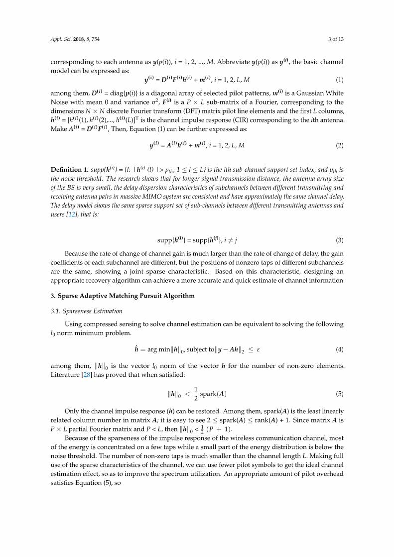
corresponding to each antenna as y(p(i)), i = 1, 2, ..., M. Abbreviate y(p(i)) as y(i), the basic channelmodel can be expressed as:

y(i) = D(i)F(i)h(i) + m(i), i = 1, 2, L, M (1)

among them, D(i) = diag{p(i)} is a diagonal array of selected pilot patterns, m(i) is a Gaussian WhiteNoise with mean 0 and variance σ2, F(i) is a P × L sub-matrix of a Fourier, corresponding to thedimensions N × N discrete Fourier transform (DFT) matrix pilot line elements and the first L columns,h(i) = [h(i)(1), h(i)(2),..., h(i)(L)]T is the channel impulse response (CIR) corresponding to the ith antenna.Make A(i) = D(i)F(i), Then, Equation (1) can be further expressed as:

y(i) = A(i)h(i) + m(i), i = 1, 2, L, M (2)

Definition 1. supp{h(i)} = {l: |h(i) (l) |> pth, 1 ≤ l ≤ L} is the ith sub-channel support set index, and pth isthe noise threshold. The research shows that for longer signal transmission distance, the antenna array sizeof the BS is very small, the delay dispersion characteristics of subchannels between different transmitting andreceiving antenna pairs in massive MIMO system are consistent and have approximately the same channel delay.The delay model shows the same sparse support set of sub-channels between different transmitting antennas andusers [12], that is:

supp{h(i)} = supp{h(j)}, i 6= j (3)

Because the rate of change of channel gain is much larger than the rate of change of delay, the gaincoefficients of each subchannel are different, but the positions of nonzero taps of different subchannelsare the same, showing a joint sparse characteristic. Based on this characteristic, designing anappropriate recovery algorithm can achieve a more accurate and quick estimate of channel information.

3. Sparse Adaptive Matching Pursuit Algorithm

3.1. Sparseness Estimation

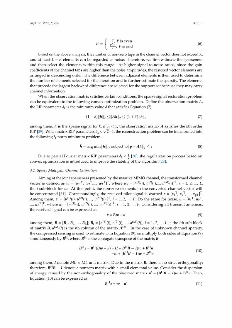
Using compressed sensing to solve channel estimation can be equivalent to solving the followingl0 norm minimum problem.

h = arg min‖h‖0, subject to‖y−Ah‖2 ≤ ε (4)

among them, ‖h‖0 is the vector l0 norm of the vector h for the number of non-zero elements.Literature [28] has proved that when satisfied:

‖h‖0 <12

spark(A) (5)

Only the channel impulse response (h) can be restored. Among them, spark(A) is the least linearlyrelated column number in matrix A; it is easy to see 2 ≤ spark(A) ≤ rank(A) + 1. Since matrix A isP × L partial Fourier matrix and P < L, then ‖h‖0 < 1

2 (P + 1).Because of the sparseness of the impulse response of the wireless communication channel, most

of the energy is concentrated on a few taps while a small part of the energy distribution is below thenoise threshold. The number of non-zero taps is much smaller than the channel length L. Making fulluse of the sparse characteristics of the channel, we can use fewer pilot symbols to get the ideal channelestimation effect, so as to improve the spectrum utilization. An appropriate amount of pilot overheadsatisfies Equation (5), so

Appl. Sci. 2018, 8, 754 4 of 13

K =

{P2 , P is even

P+12 , P is odd

(6)

Based on the above analysis, the number of non-zero taps in the channel vector does not exceed K,and at least L − K elements can be regarded as noise. Therefore, we first estimate the sparsenessand then select the elements within this range. At higher signal-to-noise ratios, since the gaincoefficients of the channel taps are higher than the noise amplitudes, the restored vector elements arearranged in descending order. The difference between adjacent elements is then used to determinethe number of elements selected for this iteration and to further estimate the sparsity. The elementsthat precede the largest backward difference are selected for the support set because they may carrychannel information.

When the observation matrix satisfies certain conditions, the sparse signal restoration problemcan be equivalent to the following convex optimization problem. Define the observation matrix A,the RIP parameter δk is the minimum value δ that satisfies Equation (7):

(1− δ)‖h‖2 ≤‖Ah‖2 ≤ (1 + δ)‖h‖2 (7)

among them, h is the sparse signal for k, if δk < 1, the observation matrix A satisfies the kth orderRIP [29]. When matrix RIP parameters δk <

√2−1, the reconstruction problem can be transformed into

the following l1 norm minimum problem.

h = arg min‖h‖1, subject to‖y−Ah‖2 ≤ ε (8)

Due to partial Fourier matrix RIP parameters δk < 12 [30], the regularization process based on

convex optimization is introduced to improve the stability of the algorithm [23].

3.2. Sparse Multipath Channel Estimation

Aiming at the joint sparseness presented by the massive MIMO channel, the transformed channelvector is defined as w = [w1

T, w2T,..., wL

T]T, where wi = [h(1)(i), h(2)(i),..., h(M)(i)]T, i = 1, 2, ..., L,the i sub-block for w. At this point, the non-zero elements in the converted channel vector willbe concentrated [31]. Correspondingly, the received pilot signal is warped z = [z1

T, z2T, ..., zpT]T.

Among them, zi = [y(1)(i), y(2)(i), ..., y(M)(i) ]T, i = 1, 2, ..., P. Do the same for noise, n = [n1T, n2

T,..., nP

T]T, where ni = [m(1)(i), m(2)(i), ..., m(M)(i)]T, i = 1, 2, ..., P. Considering all transmit antennas,the received signal can be expressed as:

z = Bw + n (9)

among them, B = [B1, B2, ..., BL]; Bi = [a(1)(i), a(2)(i), ..., a(M)(i)], i = 1, 2, ..., L is the ith sub-blockof matrix B, a(M)(i) is the ith column of the matrix A(M). In the case of unknown channel sparsity,the compressed sensing is used to estimate w in Equation (9), so multiply both sides of Equation (9)simultaneously by BH, where BH is the conjugate transpose of the matrix B.

BHz = BH(Bw + n) = (I + BHB − I)w + BHn=w + (BHB − I)w + BHn

(10)

among them, I denote ML × ML unit matrix. Due to the matrix B, there is no strict orthogonality;therefore, BHB − I denote a nonzero matrix with a small elemental value. Consider the dispersionof energy caused by the non-orthogonality of the observed matrix n′ = (BHB − I)w + BHn, Then,Equation (10) can be expressed as:

BHz = w + n’ (11)

Appl. Sci. 2018, 8, 754 5 of 13

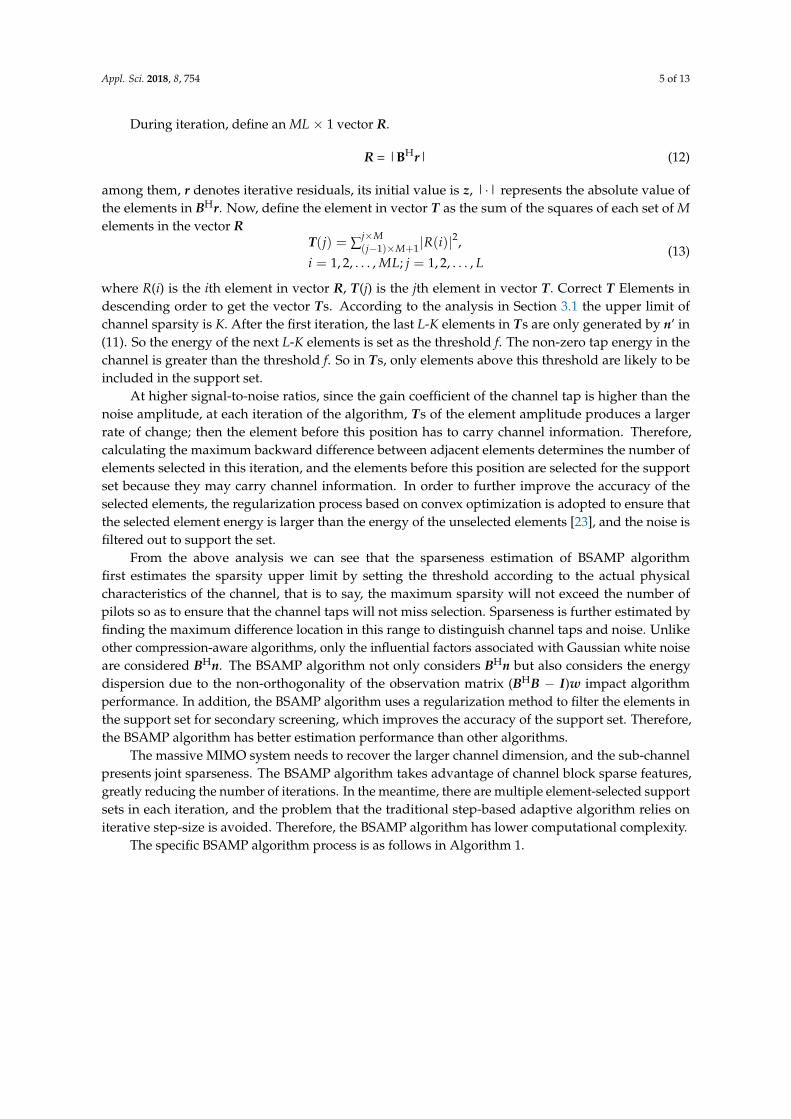
During iteration, define an ML × 1 vector R.

R = |BHr| (12)

among them, r denotes iterative residuals, its initial value is z, |·| represents the absolute value ofthe elements in BHr. Now, define the element in vector T as the sum of the squares of each set of Melements in the vector R

T(j) = ∑j×M(j−1)×M+1|R(i)|

2,

i = 1, 2, . . . , ML; j = 1, 2, . . . , L(13)

where R(i) is the ith element in vector R, T(j) is the jth element in vector T. Correct T Elements indescending order to get the vector Ts. According to the analysis in Section 3.1 the upper limit ofchannel sparsity is K. After the first iteration, the last L-K elements in Ts are only generated by n’ in(11). So the energy of the next L-K elements is set as the threshold f. The non-zero tap energy in thechannel is greater than the threshold f. So in Ts, only elements above this threshold are likely to beincluded in the support set.

At higher signal-to-noise ratios, since the gain coefficient of the channel tap is higher than thenoise amplitude, at each iteration of the algorithm, Ts of the element amplitude produces a largerrate of change; then the element before this position has to carry channel information. Therefore,calculating the maximum backward difference between adjacent elements determines the number ofelements selected in this iteration, and the elements before this position are selected for the supportset because they may carry channel information. In order to further improve the accuracy of theselected elements, the regularization process based on convex optimization is adopted to ensure thatthe selected element energy is larger than the energy of the unselected elements [23], and the noise isfiltered out to support the set.

From the above analysis we can see that the sparseness estimation of BSAMP algorithmfirst estimates the sparsity upper limit by setting the threshold according to the actual physicalcharacteristics of the channel, that is to say, the maximum sparsity will not exceed the number ofpilots so as to ensure that the channel taps will not miss selection. Sparseness is further estimated byfinding the maximum difference location in this range to distinguish channel taps and noise. Unlikeother compression-aware algorithms, only the influential factors associated with Gaussian white noiseare considered BHn. The BSAMP algorithm not only considers BHn but also considers the energydispersion due to the non-orthogonality of the observation matrix (BHB − I)w impact algorithmperformance. In addition, the BSAMP algorithm uses a regularization method to filter the elements inthe support set for secondary screening, which improves the accuracy of the support set. Therefore,the BSAMP algorithm has better estimation performance than other algorithms.

The massive MIMO system needs to recover the larger channel dimension, and the sub-channelpresents joint sparseness. The BSAMP algorithm takes advantage of channel block sparse features,greatly reducing the number of iterations. In the meantime, there are multiple element-selected supportsets in each iteration, and the problem that the traditional step-based adaptive algorithm relies oniterative step-size is avoided. Therefore, the BSAMP algorithm has lower computational complexity.

The specific BSAMP algorithm process is as follows in Algorithm 1.

Appl. Sci. 2018, 8, 754 6 of 13

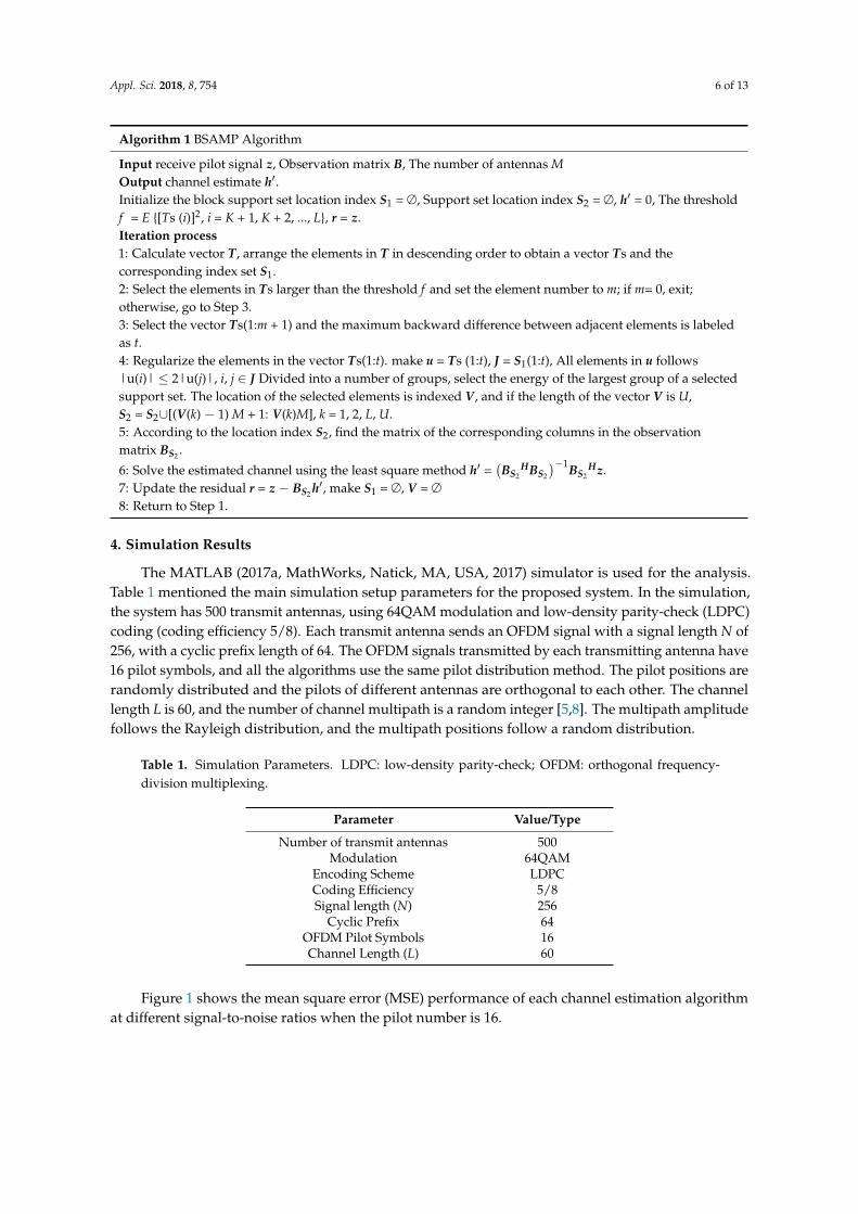
Algorithm 1 BSAMP Algorithm

Input receive pilot signal z, Observation matrix B, The number of antennas MOutput channel estimate h′.Initialize the block support set location index S1 = ∅, Support set location index S2 = ∅, h′ = 0, The thresholdf = E {[Ts (i)]2, i = K + 1, K + 2, ..., L}, r = z.Iteration process1: Calculate vector T, arrange the elements in T in descending order to obtain a vector Ts and thecorresponding index set S1.2: Select the elements in Ts larger than the threshold f and set the element number to m; if m= 0, exit;otherwise, go to Step 3.3: Select the vector Ts(1:m + 1) and the maximum backward difference between adjacent elements is labeledas t.4: Regularize the elements in the vector Ts(1:t). make u = Ts (1:t), J = S1(1:t), All elements in u follows|u(i)| ≤ 2|u(j)|, i, j ∈ J Divided into a number of groups, select the energy of the largest group of a selectedsupport set. The location of the selected elements is indexed V , and if the length of the vector V is U,S2 = S2∪[(V(k) − 1) M + 1: V(k)M], k = 1, 2, L, U.5: According to the location index S2, find the matrix of the corresponding columns in the observationmatrix BS2 .

6: Solve the estimated channel using the least square method h′ =(BS2

HBS2

)−1BS2Hz.

7: Update the residual r = z − BS2 h′, make S1 = ∅, V = ∅8: Return to Step 1.

4. Simulation Results

The MATLAB (2017a, MathWorks, Natick, MA, USA, 2017) simulator is used for the analysis.Table 1 mentioned the main simulation setup parameters for the proposed system. In the simulation,the system has 500 transmit antennas, using 64QAM modulation and low-density parity-check (LDPC)coding (coding efficiency 5/8). Each transmit antenna sends an OFDM signal with a signal length N of256, with a cyclic prefix length of 64. The OFDM signals transmitted by each transmitting antenna have16 pilot symbols, and all the algorithms use the same pilot distribution method. The pilot positions arerandomly distributed and the pilots of different antennas are orthogonal to each other. The channellength L is 60, and the number of channel multipath is a random integer [5,8]. The multipath amplitudefollows the Rayleigh distribution, and the multipath positions follow a random distribution.

Table 1. Simulation Parameters. LDPC: low-density parity-check; OFDM: orthogonal frequency-division multiplexing.

Parameter Value/Type

Number of transmit antennas 500Modulation 64QAM

Encoding Scheme LDPCCoding Efficiency 5/8Signal length (N) 256

Cyclic Prefix 64OFDM Pilot Symbols 16Channel Length (L) 60

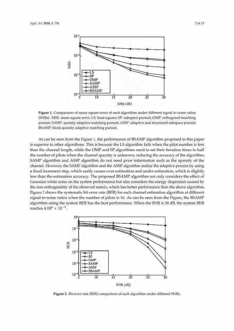
Figure 1 shows the mean square error (MSE) performance of each channel estimation algorithmat different signal-to-noise ratios when the pilot number is 16.

Appl. Sci. 2018, 8, 754 7 of 13

Appl. Sci. 2018, 8, x FOR PEER REVIEW 6 of 13

4. Simulation Results

The MATLAB (2017a, MathWorks, Natick, MA, USA, 2017) simulator is used for the analysis.

Table 1 mentioned the main simulation setup parameters for the proposed system. In the simulation,

the system has 500 transmit antennas, using 64QAM modulation and low-density parity-check

(LDPC) coding (coding efficiency 5/8). Each transmit antenna sends an OFDM signal with a signal

length N of 256, with a cyclic prefix length of 64. The OFDM signals transmitted by each transmitting

antenna have 16 pilot symbols, and all the algorithms use the same pilot distribution method. The

pilot positions are randomly distributed and the pilots of different antennas are orthogonal to each

other. The channel length L is 60, and the number of channel multipath is a random integer [5,8]. The

multipath amplitude follows the Rayleigh distribution, and the multipath positions follow a random

distribution.

Table 1. Simulation Parameters. LDPC: low-density parity-check; OFDM: orthogonal

frequency-division multiplexing.

Parameter Value/Type

Number of transmit antennas 500

Modulation 64QAM

Encoding Scheme LDPC

Coding Efficiency 5/8

Signal length (N) 256

Cyclic Prefix 64

OFDM Pilot Symbols 16

Channel Length (L) 60

Figure 1 shows the mean square error (MSE) performance of each channel estimation algorithm

at different signal-to-noise ratios when the pilot number is 16.

Figure 1. Comparison of mean square error of each algorithm under different signal to noise ratios

(SNRs). MSE: mean square error; LS: least-square; SP: subspace pursuit; OMP: orthogonal matching

pursuit; SAMP: sparsity adaptive matching pursuit; ASSP: adaptive and structured subspace

pursuit; BSAMP: block sparsity adaptive matching pursuit.

Figure 1. Comparison of mean square error of each algorithm under different signal to noise ratios(SNRs). MSE: mean square error; LS: least-square; SP: subspace pursuit; OMP: orthogonal matchingpursuit; SAMP: sparsity adaptive matching pursuit; ASSP: adaptive and structured subspace pursuit;BSAMP: block sparsity adaptive matching pursuit.

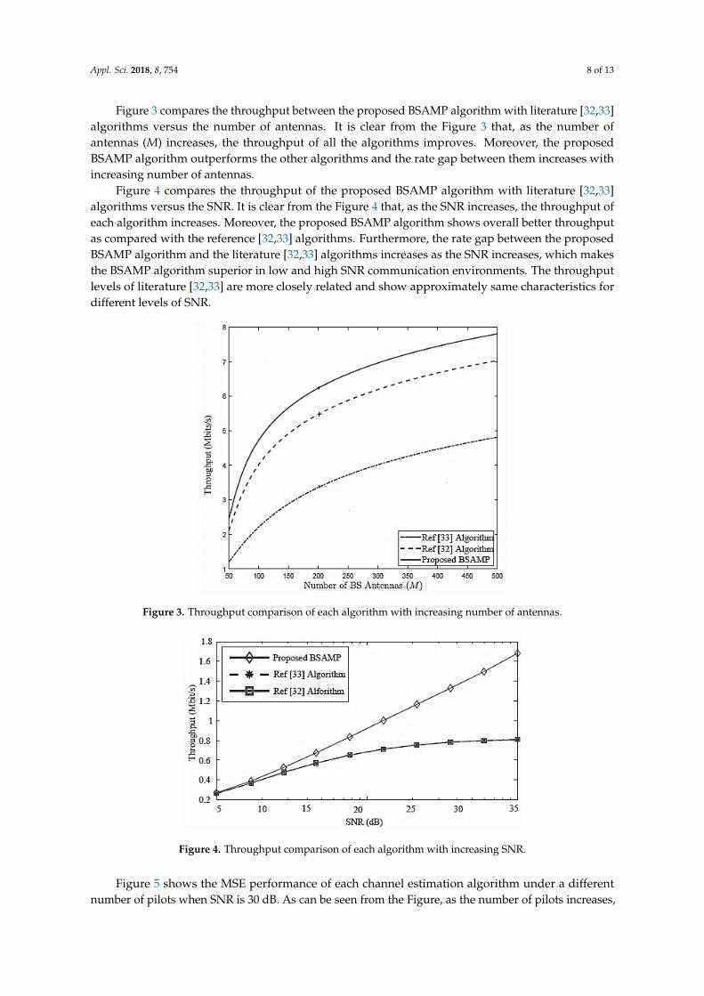
As can be seen from the Figure 1, the performance of BSAMP algorithm proposed in this paperis superior to other algorithms. This is because the LS algorithm fails when the pilot number is lessthan the channel length, while the OMP and SP algorithms need to set their iteration times to halfthe number of pilots when the channel sparsity is unknown, reducing the accuracy of the algorithm.SAMP algorithm and ASSP algorithm do not need prior information such as the sparsity of thechannel. However, the SAMP algorithm and the ASSP algorithm realize the adaptive process by usinga fixed increment step, which easily causes over-estimation and under-estimation, which is slightlyless than the estimation accuracy. The proposed BSAMP algorithm not only considers the effect ofGaussian white noise on the system performance but also considers the energy dispersion caused bythe non-orthogonality of the observed matrix, which has better performance than the above algorithm.Figure 2 shows the systematic bit error rate (BER) for each channel estimation algorithm at differentsignal-to-noise ratios when the number of pilots is 16. As can be seen from the Figure, the BSAMPalgorithm using the system BER has the best performance. When the SNR is 30 dB, the system BERreaches 4.187 × 10−5.

Appl. Sci. 2018, 8, x FOR PEER REVIEW 7 of 13

As can be seen from the Figure 1, the performance of BSAMP algorithm proposed in this paper

is superior to other algorithms. This is because the LS algorithm fails when the pilot number is less

than the channel length, while the OMP and SP algorithms need to set their iteration times to half the

number of pilots when the channel sparsity is unknown, reducing the accuracy of the algorithm.

SAMP algorithm and ASSP algorithm do not need prior information such as the sparsity of the

channel. However, the SAMP algorithm and the ASSP algorithm realize the adaptive process by

using a fixed increment step, which easily causes over-estimation and under-estimation, which is

slightly less than the estimation accuracy. The proposed BSAMP algorithm not only considers the

effect of Gaussian white noise on the system performance but also considers the energy dispersion

caused by the non-orthogonality of the observed matrix, which has better performance than the

above algorithm. Figure 2 shows the systematic bit error rate (BER) for each channel estimation

algorithm at different signal-to-noise ratios when the number of pilots is 16. As can be seen from the

Figure, the BSAMP algorithm using the system BER has the best performance. When the SNR is 30

dB, the system BER reaches 4.187 × 10−5.

Figure 2. Bit error rate (BER) comparison of each algorithm under different SNRs.

Figure 3 compares the throughput between the proposed BSAMP algorithm with literature

[32,33] algorithms versus the number of antennas. It is clear from the Figure 3 that, as the number of

antennas (M) increases, the throughput of all the algorithms improves. Moreover, the proposed

BSAMP algorithm outperforms the other algorithms and the rate gap between them increases with

increasing number of antennas.

Figure 4 compares the throughput of the proposed BSAMP algorithm with literature [32,33]

algorithms versus the SNR. It is clear from the Figure 4 that, as the SNR increases, the throughput of

each algorithm increases. Moreover, the proposed BSAMP algorithm shows overall better throughput

as compared with the reference [32,33] algorithms. Furthermore, the rate gap between the proposed

BSAMP algorithm and the literature [32,33] algorithms increases as the SNR increases, which makes

the BSAMP algorithm superior in low and high SNR communication environments. The throughput

levels of literature [32,33] are more closely related and show approximately same characteristics for

different levels of SNR.

Figure 2. Bit error rate (BER) comparison of each algorithm under different SNRs.

Appl. Sci. 2018, 8, 754 8 of 13

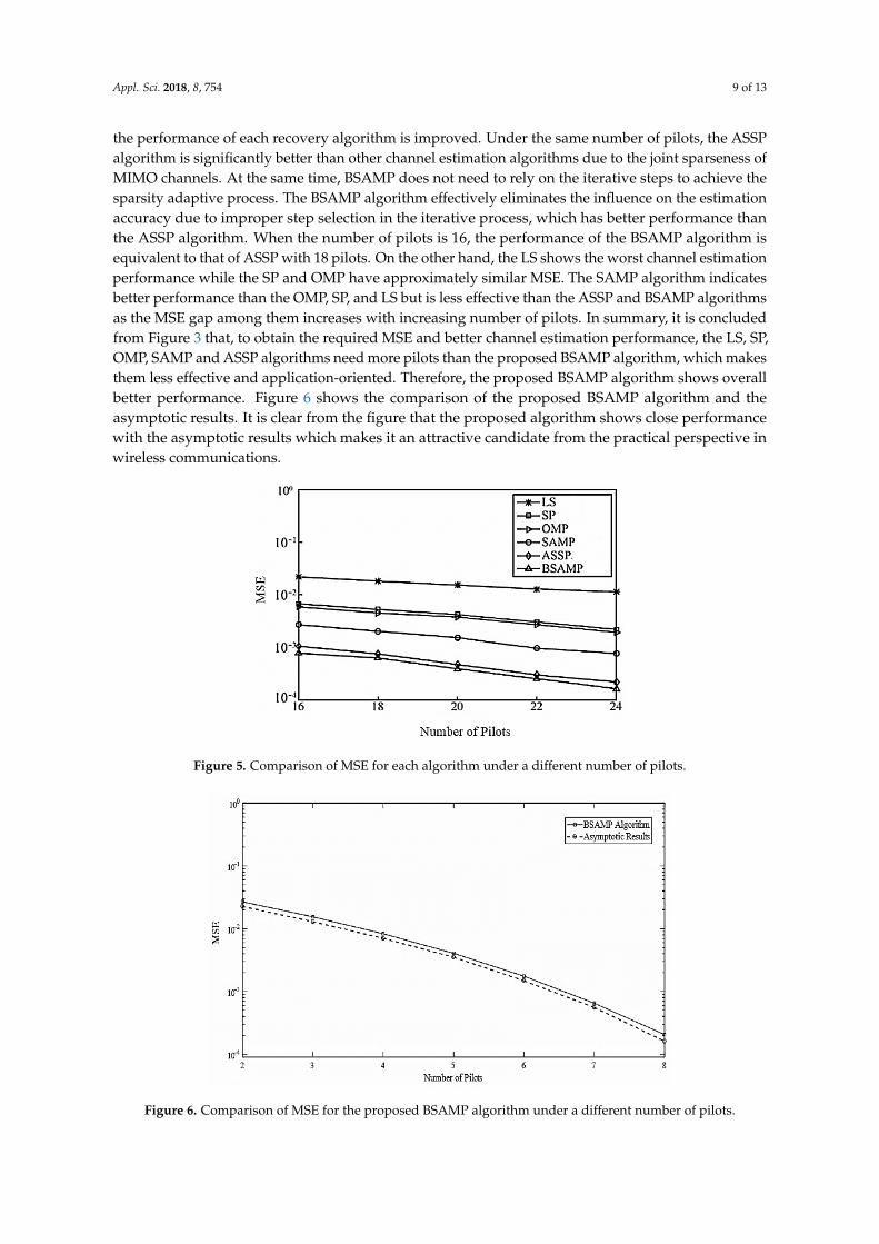
Figure 3 compares the throughput between the proposed BSAMP algorithm with literature [32,33]algorithms versus the number of antennas. It is clear from the Figure 3 that, as the number ofantennas (M) increases, the throughput of all the algorithms improves. Moreover, the proposedBSAMP algorithm outperforms the other algorithms and the rate gap between them increases withincreasing number of antennas.

Figure 4 compares the throughput of the proposed BSAMP algorithm with literature [32,33]algorithms versus the SNR. It is clear from the Figure 4 that, as the SNR increases, the throughput ofeach algorithm increases. Moreover, the proposed BSAMP algorithm shows overall better throughputas compared with the reference [32,33] algorithms. Furthermore, the rate gap between the proposedBSAMP algorithm and the literature [32,33] algorithms increases as the SNR increases, which makesthe BSAMP algorithm superior in low and high SNR communication environments. The throughputlevels of literature [32,33] are more closely related and show approximately same characteristics fordifferent levels of SNR.Appl. Sci. 2018, 8, x FOR PEER REVIEW 8 of 13

Figure 3. Throughput comparison of each algorithm with increasing number of antennas.

Figure 4. Throughput comparison of each algorithm with increasing SNR.

Figure 5 shows the MSE performance of each channel estimation algorithm under a different

number of pilots when SNR is 30 dB. As can be seen from the Figure, as the number of pilots

increases, the performance of each recovery algorithm is improved. Under the same number of

pilots, the ASSP algorithm is significantly better than other channel estimation algorithms due to the

joint sparseness of MIMO channels. At the same time, BSAMP does not need to rely on the iterative

steps to achieve the sparsity adaptive process. The BSAMP algorithm effectively eliminates the

influence on the estimation accuracy due to improper step selection in the iterative process, which has

better performance than the ASSP algorithm. When the number of pilots is 16, the performance of

the BSAMP algorithm is equivalent to that of ASSP with 18 pilots. On the other hand, the LS shows

the worst channel estimation performance while the SP and OMP have approximately similar MSE.

The SAMP algorithm indicates better performance than the OMP, SP, and LS but is less effective

Figure 3. Throughput comparison of each algorithm with increasing number of antennas.

Appl. Sci. 2018, 8, x FOR PEER REVIEW 8 of 13

Figure 3. Throughput comparison of each algorithm with increasing number of antennas.

Figure 4. Throughput comparison of each algorithm with increasing SNR.

Figure 5 shows the MSE performance of each channel estimation algorithm under a different

number of pilots when SNR is 30 dB. As can be seen from the Figure, as the number of pilots

increases, the performance of each recovery algorithm is improved. Under the same number of

pilots, the ASSP algorithm is significantly better than other channel estimation algorithms due to the

joint sparseness of MIMO channels. At the same time, BSAMP does not need to rely on the iterative

steps to achieve the sparsity adaptive process. The BSAMP algorithm effectively eliminates the

influence on the estimation accuracy due to improper step selection in the iterative process, which has

better performance than the ASSP algorithm. When the number of pilots is 16, the performance of

the BSAMP algorithm is equivalent to that of ASSP with 18 pilots. On the other hand, the LS shows

the worst channel estimation performance while the SP and OMP have approximately similar MSE.

The SAMP algorithm indicates better performance than the OMP, SP, and LS but is less effective

Figure 4. Throughput comparison of each algorithm with increasing SNR.

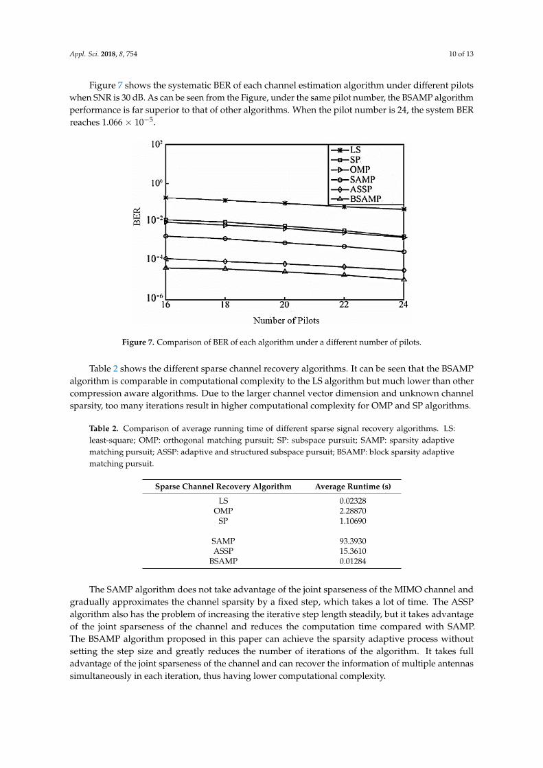
Figure 5 shows the MSE performance of each channel estimation algorithm under a differentnumber of pilots when SNR is 30 dB. As can be seen from the Figure, as the number of pilots increases,

Appl. Sci. 2018, 8, 754 9 of 13

the performance of each recovery algorithm is improved. Under the same number of pilots, the ASSPalgorithm is significantly better than other channel estimation algorithms due to the joint sparseness ofMIMO channels. At the same time, BSAMP does not need to rely on the iterative steps to achieve thesparsity adaptive process. The BSAMP algorithm effectively eliminates the influence on the estimationaccuracy due to improper step selection in the iterative process, which has better performance thanthe ASSP algorithm. When the number of pilots is 16, the performance of the BSAMP algorithm isequivalent to that of ASSP with 18 pilots. On the other hand, the LS shows the worst channel estimationperformance while the SP and OMP have approximately similar MSE. The SAMP algorithm indicatesbetter performance than the OMP, SP, and LS but is less effective than the ASSP and BSAMP algorithmsas the MSE gap among them increases with increasing number of pilots. In summary, it is concludedfrom Figure 3 that, to obtain the required MSE and better channel estimation performance, the LS, SP,OMP, SAMP and ASSP algorithms need more pilots than the proposed BSAMP algorithm, which makesthem less effective and application-oriented. Therefore, the proposed BSAMP algorithm shows overallbetter performance. Figure 6 shows the comparison of the proposed BSAMP algorithm and theasymptotic results. It is clear from the figure that the proposed algorithm shows close performancewith the asymptotic results which makes it an attractive candidate from the practical perspective inwireless communications.

Appl. Sci. 2018, 8, x FOR PEER REVIEW 9 of 13

than the ASSP and BSAMP algorithms as the MSE gap among them increases with increasing

number of pilots. In summary, it is concluded from Figure 3 that, to obtain the required MSE and

better channel estimation performance, the LS, SP, OMP, SAMP and ASSP algorithms need more

pilots than the proposed BSAMP algorithm, which makes them less effective and

application-oriented. Therefore, the proposed BSAMP algorithm shows overall better performance.

Figure 6 shows the comparison of the proposed BSAMP algorithm and the asymptotic results. It is

clear from the figure that the proposed algorithm shows close performance with the asymptotic

results which makes it an attractive candidate from the practical perspective in wireless

communications.

Figure 5. Comparison of MSE for each algorithm under a different number of pilots.

Figure 6. Comparison of MSE for the proposed BSAMP algorithm under a different number of pilots.

Figure 7 shows the systematic BER of each channel estimation algorithm under different pilots

when SNR is 30 dB. As can be seen from the Figure, under the same pilot number, the BSAMP

Figure 5. Comparison of MSE for each algorithm under a different number of pilots.

Appl. Sci. 2018, 8, x FOR PEER REVIEW 9 of 13

than the ASSP and BSAMP algorithms as the MSE gap among them increases with increasing

number of pilots. In summary, it is concluded from Figure 3 that, to obtain the required MSE and

better channel estimation performance, the LS, SP, OMP, SAMP and ASSP algorithms need more

pilots than the proposed BSAMP algorithm, which makes them less effective and

application-oriented. Therefore, the proposed BSAMP algorithm shows overall better performance.

Figure 6 shows the comparison of the proposed BSAMP algorithm and the asymptotic results. It is

clear from the figure that the proposed algorithm shows close performance with the asymptotic

results which makes it an attractive candidate from the practical perspective in wireless

communications.

Figure 5. Comparison of MSE for each algorithm under a different number of pilots.

Figure 6. Comparison of MSE for the proposed BSAMP algorithm under a different number of pilots.

Figure 7 shows the systematic BER of each channel estimation algorithm under different pilots

when SNR is 30 dB. As can be seen from the Figure, under the same pilot number, the BSAMP

Figure 6. Comparison of MSE for the proposed BSAMP algorithm under a different number of pilots.

Appl. Sci. 2018, 8, 754 10 of 13

Figure 7 shows the systematic BER of each channel estimation algorithm under different pilotswhen SNR is 30 dB. As can be seen from the Figure, under the same pilot number, the BSAMP algorithmperformance is far superior to that of other algorithms. When the pilot number is 24, the system BERreaches 1.066 × 10−5.

Appl. Sci. 2018, 8, x FOR PEER REVIEW 10 of 13

algorithm performance is far superior to that of other algorithms. When the pilot number is 24, the

system BER reaches 1.066 × 10−5.

Figure 7. Comparison of BER of each algorithm under a different number of pilots.

Table 2 shows the different sparse channel recovery algorithms. It can be seen that the BSAMP

algorithm is comparable in computational complexity to the LS algorithm but much lower than

other compression aware algorithms. Due to the larger channel vector dimension and unknown

channel sparsity, too many iterations result in higher computational complexity for OMP and SP

algorithms.

Table 2. Comparison of average running time of different sparse signal recovery algorithms. LS:

least-square; OMP: orthogonal matching pursuit; SP: subspace pursuit; SAMP: sparsity adaptive

matching pursuit; ASSP: adaptive and structured subspace pursuit; BSAMP: block sparsity adaptive

matching pursuit.

Sparse Channel Recovery Algorithm Average Runtime (s)

LS 0.02328

OMP 2.28870

SP 1.10690

SAMP 93.3930

ASSP 15.3610

BSAMP 0.01284

The SAMP algorithm does not take advantage of the joint sparseness of the MIMO channel and

gradually approximates the channel sparsity by a fixed step, which takes a lot of time. The ASSP

algorithm also has the problem of increasing the iterative step length steadily, but it takes advantage

of the joint sparseness of the channel and reduces the computation time compared with SAMP. The

BSAMP algorithm proposed in this paper can achieve the sparsity adaptive process without setting

the step size and greatly reduces the number of iterations of the algorithm. It takes full advantage of

the joint sparseness of the channel and can recover the information of multiple antennas

simultaneously in each iteration, thus having lower computational complexity.

5. Conclusions

This paper proposes a BSAMP algorithm with adaptive sparsity-based on the joint sparsity of

sub-channels in massive MIMO systems. The algorithm chooses the support elements as the first

choice by setting the threshold and finding the maximum backward difference position. The element

Figure 7. Comparison of BER of each algorithm under a different number of pilots.

Table 2 shows the different sparse channel recovery algorithms. It can be seen that the BSAMPalgorithm is comparable in computational complexity to the LS algorithm but much lower than othercompression aware algorithms. Due to the larger channel vector dimension and unknown channelsparsity, too many iterations result in higher computational complexity for OMP and SP algorithms.

Table 2. Comparison of average running time of different sparse signal recovery algorithms. LS:least-square; OMP: orthogonal matching pursuit; SP: subspace pursuit; SAMP: sparsity adaptivematching pursuit; ASSP: adaptive and structured subspace pursuit; BSAMP: block sparsity adaptivematching pursuit.

Sparse Channel Recovery Algorithm Average Runtime (s)

LS 0.02328OMP 2.28870

SP 1.10690

SAMP 93.3930ASSP 15.3610

BSAMP 0.01284

The SAMP algorithm does not take advantage of the joint sparseness of the MIMO channel andgradually approximates the channel sparsity by a fixed step, which takes a lot of time. The ASSPalgorithm also has the problem of increasing the iterative step length steadily, but it takes advantageof the joint sparseness of the channel and reduces the computation time compared with SAMP.The BSAMP algorithm proposed in this paper can achieve the sparsity adaptive process withoutsetting the step size and greatly reduces the number of iterations of the algorithm. It takes fulladvantage of the joint sparseness of the channel and can recover the information of multiple antennassimultaneously in each iteration, thus having lower computational complexity.

Appl. Sci. 2018, 8, 754 11 of 13

5. Conclusions

This paper proposes a BSAMP algorithm with adaptive sparsity-based on the joint sparsity ofsub-channels in massive MIMO systems. The algorithm chooses the support elements as the firstchoice by setting the threshold and finding the maximum backward difference position. The elementis secondarily selected by regularization to improve the accuracy of the selected elements. The MSE,BER and throughput analysis is performed against the SNR and number of pilots. The proposedBSAMP algorithm is compared with LS, OMP, SP, SAMP, ASSP, and reference [32,33] algorithms,and the corresponding system parameters are analyzed for performance evaluations. The algorithmcomplexity analysis was also performed, which clearly estimated that the proposed BSAMP algorithmhas a 0.01284 s average runtime, which is much smaller than the other algorithms such as the averageruntime of SAMP algorithm, which is 93.3930 s and the ASSP algorithm which has an averageruntime of 15.3610 s. With such a computationally-efficient behavior, the proposed BSAMP algorithmprovides efficient sparse channel estimation capability for 5G massive MIMO systems which alsoenables us to deploy it in practical usage scenarios. Theoretical analysis and simulation results showthat the BSAMP algorithm has good channel estimation performance, high throughput and lowcomputational complexity as compared to other algorithms. This research work can further beextended by incorporating the proposed BSAMP algorithm in TDD, FDD Massive MIMO for EnergyEfficiency Analysis versus different performance metrics such as the distance between the BS andmobile users, antenna element spacing and hardware impairments.

Author Contributions: Imran Khan conceived and designed the main idea, perform the experiments and wrotethe paper; Madhusudan Singh provided extensive technical support in literature survey and theoretical analysis;Dhananjay Singh provided extensive support in analysis, validation and performance evaluation of the proposedwork with existing works. He also provided support in research funding.

Acknowledgments: This research work is supported by Hankuk University of Foreign Studies research fund 2018.

Conflicts of Interest: The authors declare no conflict of interest.

References

1. Marzetta, T.L. Non-cooperative cellular wireless with unlimited numbers of base station antennas. IEEE Trans.Wirel. Commun. 2010, 9, 3590–3600. [CrossRef]

2. Shariati, N.; Bjornson, E.; Bengtsson, M.; Debbah, M. Low-complexity polynomial channel estimation inlarge-scale MIMO with arbitrary statistics. IEEE J. Sel. Top. Signal Proc. 2014, 8, 815–830. [CrossRef]

3. Wen, C.K.; Jin, S.; Wong, K.K.; Chen, J.C.; Ting, P. Channel estimation for massive MIMO usingGaussian-mixture Bayesian learning. IEEE J. Sel. Top. Signal Proc. 2014, 8, 815–830. [CrossRef]

4. Zhen, J.; Rao, B.D. Capacity analysis of MIMO systems with unknown channel state information.In Proceedings of the IEEE Information Theory Workshop, San Antonio, TX, USA, 24–29 October 2004;pp. 413–417. [CrossRef]

5. Marzetta, T.L. How much training is required for multiuser MIMO? In Proceedings of the IEEE 2006Fortieth Asilomar Conference on Signals, Systems and Computers (ACSSC), Pacific Grove, CA, USA,29 October–1 November 2006; pp. 359–363. [CrossRef]

6. Wu, S.; Kuang, L.; Ni, Z.; Huang, D.; Gao, Q.; Lu, J. Message-passing receiver for joint channel estimation anddecoding in 3D massive MIMO-OFDM systems. IEEE Trans. Wirel. Commun. 2006, 15, 8122–8138. [CrossRef]

7. Khan, I.; Zafar, M.; Jan, M.; Lloret, J.; Basheri, M.; Singh, D. Spectral and Energy Efficient Low-OverheadUplink and Downlink Channel Estimation for 5G Massive MIMO Systems. Entropy 2018, 20, 92. [CrossRef]

8. Khan, I.; Singh, D. Efficient Compressive Sensing Based Sparse Channel Estimation for 5G Massive MIMOSystems. AEUE Int. J. Electron. Commun. 2018, 89, 181–190. [CrossRef]

9. Masood, M.; Afify, L.H.; Al-Naffouri, T.Y. Efficient Coordinated Recovery of Sparse Channels in MassiveMIMO. IEEE Trans. Signal Proc. 2014, 63, 104–118. [CrossRef]

Appl. Sci. 2018, 8, 754 12 of 13

10. Kulsoom, F.; Vizziello, A.; Chaudhry, H.N.; Savazzi, P. Pilot reduction techniques for sparse channelestimation in massive MIMO systems. In Proceedings of the 2018 14th Annual Conference on WirelessOn-demand Network Systems and Services (WONS), Isola, France, 6–8 February 2018; pp. 111–116.[CrossRef]

11. Liu, L.; Huang, C.; Chi, Y.; Yuen, C.; Guan, Y.L.; Li, Y. Sparse Vector Recovery: Bernoulli-Gaussian MessagePassing. In Proceedings of the 2017 IEEE Global Communications Conference, Singapore, 4–8 December2017; pp. 1–6. [CrossRef]

12. Huang, C.; Liu, L.; Yuen, C.; Sun, S. A LSE and Sparse Message Passing-Based Channel Estimation formmWave MIMO Systems. In Proceedings of the 2016 IEEE Global Communications Conference, Washington,DC, USA, 4–8 December 2016; pp. 1–6. [CrossRef]

13. Li, J.; Yuen, C.; Li, D.; Zhang, H.; Wu, X. On hybrid Pilot for Channel Estimation in Massive MIMO Uplink.2018. Available online: https://arxiv.org/abs/1608.02112 (accessed on 2 March 2018).

14. Gao, Z.; Dai, L.; Mi, D.; Wang, Z.; Imran, M.A.; Shakir, M.Z. MmWave massive-MIMO-based wirelessbackhaul for the 5G ultra-dense network. IEEE Wirel. Commun. 2015, 22, 13–21. [CrossRef]

15. Qi, C.; Huang, Y.; Jin, S.; Wu, L. Sparse channel estimation based on compressed sensing for massive MIMOsystems. In Proceedings of the IEEE International Conference on Communications (ICC), London, UK,8–12 June 2015; pp. 4558–4563. [CrossRef]

16. Zheng, Z.; Hao, C.Y.; Yang, X.M. Least squares channel estimation with noise suppression for OFDM systems.Electr. Lett. 2016, 52, 37–39. [CrossRef]

17. Lin, B.J.; Tang, X.; Ghassemlooy, Z.; Zhang, S.; Li, Y.; Wu, Y.; Li, H. Efficient frequency-domain channelequalization methods for OFDM visible light communications. IET Commun. 2017, 11, 25–29. [CrossRef]

18. Kalakech, A.; Berbineau, M.; Dayoub, I.; Simon, E.P. Time-domain LMMSE channel estimator based onsliding window for OFDM systems in high-mobility situations. IEEE Trans. Veh. Technol. 2015, 64, 5728–5740.[CrossRef]

19. Cramer, R.J.M.; Scholtz, R.A.; Win, M.Z. Evaluation of an ultra-wide-band propagation channel. IEEE Trans.Antennas Propag. 2002, 50, 561–570. [CrossRef]

20. Pardes, J.L.; Arce, G.R.; Wang, Z.M. Ultra-wideband compressed sensing: Channel estimation. IEEE J. Sel. Top.Signal Process. 2007, 1, 383–395. [CrossRef]

21. Seo, J.; Jang, S.; Yang, J.; Jeon, W.; Kim, D.K. Analysis of pilot-aided channel estimation with optimal leakagesuppression for OFDM systems. IEEE Commun. Lett. 2010, 14, 809–811. [CrossRef]

22. Cai, T.T.; Wang, L. The orthogonal matching pursuit for sparse signal recovery with noise. IEEE Trans.Inf. Theory 2011, 57, 4680–4688. [CrossRef]

23. Uwaechia, A.N.; Mahyuddin, N.M. A Review on Sparse Channel Estimation in OFDM System UsingCompressed Sensing. IETE Tech. Rev. 2017, 34, 514–531. [CrossRef]

24. Zu, B.K.; Xia, X.Y.; Xia, K.W.; Bai, C. Channel estimation on 60 GHz wireless communication system basedon subspace pursuit. J. Comput. Inf. Syst. 2014, 10, 10565–10572.

25. Zhang, Y.; Venkates, R.; Dobre, O.A.; Li, C. An adaptive matching pursuit algorithm for sparse channelestimation. In Proceedings of the IEEE Wireless Communications and Networking Conference (WCNC2015), New Orleans, LA, USA, 9–12 March 2015; pp. 626–630. [CrossRef]

26. Barbotin, Y.; Hormati, A.; Rangan, S.; Vetterli, M. Estimation of sparse MIMO channels with common support.IEEE Trans. Commun. 2012, 60, 3705–3716. [CrossRef]

27. Gao, Z.; Dai, L.L.; Dai, W.; Shim, B.; Wang, Z. Structured compressive sensing-based spatio-temporal jointchannel estimation for FDD massive MIMO. IEEE Trans. Commun. 2016, 64, 601–617. [CrossRef]

28. David, L.D.; Michael, E. Optimally sparse representation in general (nonorthogonal) dictionaries via l1minimization. Proc. Natl. Acad. Sci. USA 2003, 100, 2197–2202. [CrossRef]

29. Candes, E.; Tao, T. Decoding by linear programming. IEEE Trans. Inf. Theory 2005, 51, 4203–4215. [CrossRef]30. Candes, E.; Romberg, J.; Tao, T. Robust uncertainty principles: Exact signal reconstruction from highly

incomplete Fourier information. IEEE Trans. Inf. Theory 2006, 52, 489–509. [CrossRef]31. Duarte, M.; Eldar, Y. Structured compressed sensing: From theory to applications. IEEE Trans. Signal Proc.

2009, 59, 4053–4085. [CrossRef]

Appl. Sci. 2018, 8, 754 13 of 13

32. Gao, Z.; Dai, L.; Wang, Z.; Chen, S. Spatially Common Sparsity Based Adaptive Channel Estimation andFeedback for FDD Massive MIMO. IEEE Trans. Signal Proc. 2015, 63, 6169–6183. [CrossRef]

33. Wunder, G.; Boche, H.; Strohmer, T.; Jung, P. Sparse Signal Processing Concepts for Efficient 5G SystemDesign. IEEE Access 2015, 3, 195–208. [CrossRef]

© 2018 by the authors. Licensee MDPI, Basel, Switzerland. This article is an open accessarticle distributed under the terms and conditions of the Creative Commons Attribution(CC BY) license (http://creativecommons.org/licenses/by/4.0/).