Compressive sensing algorithms applied to stator … · Compressive sensing algorithms applied to stator current signal From 02/03/2015 to 07/08/2015 Under the supervision of: ...

Rose MAZARI

SICOM

2015

Laboratory of Multimedia Signal and Systems

Adr: Dzordza Vasingtona bb-Podgorica-MONTENEGRO

Compressive sensing algorithms applied to stator current signal

From 02/03/2015 to 07/08/2015

Under the supervision of:

- Company supervisor : Irena OROVIC - [email protected] - Phelma Tutor: Cornel IOANA – [email protected] -

Confidentiality : no

Ecole nationale

supérieure de physique,

électronique, matériaux

Phelma

Bât. Grenoble INP - Minatec

3 Parvis Louis Néel - CS 50257

F-38016 Grenoble Cedex 01

Tél +33 (0)4 56 52 91 00

Fax +33 (0)4 56 52 91 03

http://phelma.grenoble-inp.fr

mailto:[email protected]

mailto:[email protected]

Rose Mazari - École Nationale Supérieure de l’énergie, l’eau et l’environnement (ENSE3) -2014/2015 2

COMPRESSIVE SENSING ALGORITHMS APPLIED TO CURRENT SIGNALS

ACKNOWLEDGMENTS

This project would not have been possible without the support of many people.

I therefore express my gratitude to my supervisor Ms. Irena Orovic whose advices, understanding and patience are fully appreciated. I am grateful towards Pr. Srdjan Stankovic for sharing his experience with us as well on the scientific side as concerning the history of Montenegro.

I would like to thank Ms. Andjela Draganic and Ms. Maja Lakicevic for being here for us every single time I needed them and for giving us tips about the most beautiful places to visit in Montenegro.

I am grateful towards my Professor Cornel Ioana who made the internship possible and took care of us on the whole internship period.

And I would also like to thank Emile Devillers my partner at work and life; we won’t forget this great experience.

Thank you to everyone for you warm hospitality, Montenegro is a wonderful country with plenty of wonderful people.



SUMMARY

ACKNOWLEDGMENTS ______________________________________________________________________________ 2

SUMMARY _______________________________________________________________________________________ 3

Glossary_________________________________________________________________________________________ 4

Illustration Tab ___________________________________________________________________________________ 5

Introducing the Laboratory __________________________________________________________________________ 6

Introduction _____________________________________________________________________________________ 7

1. An introduction to compressive sensing ___________________________________________________________ 8

2. General principle of compressive sensing _________________________________________________________ 10

a) Mathematical representation ________________________________________________________________ 10

b) Concept of incoherent sampling ______________________________________________________________ 10

c) The Restricted Isometry Property _____________________________________________________________ 11

d) Problem Statement ________________________________________________________________________ 11

3. Gradient Based reconstruction __________________________________________________________________ 12

a) Gradient Based Algorithm principle ___________________________________________________________ 12

b) Gradient Based algorithm (GBA) ______________________________________________________________ 14

4. Gradient Based algorithm results ________________________________________________________________ 16

a) Sinus reconstruction using the gradient based algorithm ___________________________________________ 16

b) Gradient Based algorithm applied to the stator current ____________________________________________ 20

c) Extension of the GBA to the images ___________________________________________________________ 22

5. General Deviation algorithm ___________________________________________________________________ 23

a) General Deviation principles _________________________________________________________________ 23

b) General Deviation Algorithm _________________________________________________________________ 26

6. Results of the General Deviation Algorithm ________________________________________________________ 28

a) Theoretical framework _____________________________________________________________________ 28

b) First example _____________________________________________________________________________ 28

c) Second example ___________________________________________________________________________ 30

d) General deviation algorithm applied to the stator current __________________________________________ 32

CONCLUSION____________________________________________________________________________________ 35

Bibliography ____________________________________________________________________________________ 36

ANNEX A _______________________________________________________________________________________ 38

ANNEX B _______________________________________________________________________________________ 41



Glossary

𝐹𝑒 : Sampling Frequency

𝐹𝑚𝑎𝑥 : Highest Frequency in the signal

𝑘 : Number of non-zero coefficients

𝑛 : Signal’s length

𝛹 ℝn*n the matrix from the basis in which 𝑥 has the best sparse representation

𝑋 ∈ ℝn is the best sparse representation from 𝑥 in the basis 𝛹.

𝛷 ∈ ℝm*n the sampling matrix allowing to have only 𝑚 measurements from the initial vector 𝑥

𝜃 = 𝛷𝛹 𝜇(𝛷,𝛹): Coherence measurement

∑ |𝑋|𝑝𝑁−1𝑘=0 𝐿𝑝-norm

𝑀1 : Concentration measurements with the 𝑙1-norm

𝛽𝑚: the gradient’s angle between two successive values 𝑔𝑚−1(𝑛) and 𝑔𝑚(𝑛)

𝑇𝑟 : Stopping criterion

𝛥 : Step of the Gradient Based Algorithm

𝐼 : Total error

𝐺𝐷 : General Deviation



Illustration Tab

FIGURE 1 IMAGE TAKEN WITH THE SINGLE PIXEL CAMERA. ...................................................................................................................................... 9

FIGURE 2 (A) COMPRESSIVE SENSING MEASUREMENT PROCESS WITH A RANDOM GAUSSIAN MEASUREMENT MATRIX 𝜱 AND A DCT MATRIX. (B) MEASUREMENT PROCESS WITH 𝜽 = 𝜱𝜳. THERE ARE FOUR COLUMNS THAT CORRESPOND TO NON-ZERO SI COEFFICIENTS. THE MEASUREMENT VECTOR 𝒚 IS A LINEAR

COMBINATION OF THESE COLUMNS. ....................................................................................................................................................... 10

FIGURE 3 MEASURE OF THE L1-NORM AS A FUNCTION OF MISSING SAMPLES ........................................................................................................... 13

FIGURE 4 ORIGINAL SIGNAL ........................................................................................................................................................................... 16

FIGURE 5 ORIGINAL SIGNAL WITH 95% MISSING SAMPLE ..................................................................................................................................... 16

FIGURE 6 DIFFERENCE BETWEEN THE INITIAL SIGNAL AND THE RECONSTRUCTED ONE. ALGORITHM PERFORMED IN THE DFT DOMAIN UNTIL 100 ITERATIONS .. 17

FIGURE 8 COMPARISON BETWEEN DFT & DCT SPARSE DOMAIN ........................................................................................................................... 18

FIGURE 7 DIFFERENCE BETWEEN THE ORIGINAL SIGNAL AND THE RECONSTRUCTED ONE ALGORITHM PERFORMED IN THE DCT DOMAIN UNTIL 100 ITERATIONS 18

FIGURE 9 ALGORITHM IMPROVEMENT ............................................................................................................................................................. 19

FIGURE 10 EVOLUTION OF BETA FOR (A) Δ = MAX(Y(N)) AND (B) Δ =3* MAX(Y(N)) ................................................................................................. 19

FIGURE 11 (A) STATOR CURRENT IAJ03 LABEL AXIS=SAMPLE (B) STATOR CURRENT FOURIER TRANSFORM ON A LOGARITHMIC SCALE .................................. 20

FIGURE 12 LOGARITHMIC DFT OF THE STATOR CURRENT ..................................................................................................................................... 21

FIGURE 13 LOGARITHMIC DFT OF THE STATOR CURRENT AFTER SPASIFICATION ........................................................................................................ 21

FIGURE 14 RECONSTRUCTION ERROR BETWEEN THE ORIGINAL SIGNAL X0 AND THE RECOVERED ONE XR ........................................................................ 21

FIGURE 15 IN BLUE THE EXTRACTED RSH COMPONENT FROM THE RECOVERED CURRENT SIGNAL- IN GREEN THE THEORITICAL SPEED ................................... 21

FIGURE 16 GBA PERFORMED ON A LOW FREQUENCY IMAGE IN THE DFT DOMAIN .................................................................................................... 22

FIGURE 17 GBA PERFORMED ON A LOW FREQUENCY IMAGE IN THE DCT DOMAIN .................................................................................................... 22

FIGURE 18 (A) ORIGINAL SIGNAL X(N). (B) ORIGINAL SIGNAL WITH A GAUSSIAN NOISE WITH SIGMA = 0 AND AVERAGE = 0. (C) ORIGINAL SIGNAL WITH 85% OF REMOVED SAMPLES. (D) RECOVERY OF THE INITIAL SIGNAL. ......................................................................................................................... 28

FIGURE 19 GENERAL DEVIATION COMPUTATION FOR AN L2 NORM ....................................................................................................................... 29

FIGURE 20 (A) ORIGINAL SIGNAL X(N). (B) ORIGINAL SIGNAL WITH A GAUSSIAN NOISE WITH SIGMA = 0,5 AND AVERAGE = 0. (C) ORIGINAL SIGNAL WITH 85% OF REMOVED SAMPLES. (D) RECOVERY OF THE INITIAL SIGNAL WITH AN L2 NORM. .......................................................................................... 30

FIGURE 21 (A) ORIGINAL SIGNAL X(N). (B) ORIGINAL SIGNAL WITH A GAUSSIAN NOISE WITH SIGMA = 0,5 AND AVERAGE = 0. (C) ORIGINAL SIGNAL WITH 85%

OF REMOVED SAMPLES. (D) RECOVERY OF THE INITIAL SIGNAL WITH AN L1 NORM. .......................................................................................... 30

FIGURE 22 (A) ORIGINAL SIGNAL X(N). (B) ORIGINAL SIGNAL WITH 3 IMPULSION NOISE. (C) ORIGINAL SIGNAL WITH 85% OF REMOVED SAMPLES. (D) RECOVERY OF THE INITIAL SIGNAL WITH AN L1 NORM. .............................................................................................................................................. 31

FIGURE 23 (A) ORIGINAL SIGNAL X(N). (B) ORIGINAL SIGNAL WITH 3 IMPULSION NOISE. (C) ORIGINAL SIGNAL WITH 85% OF REMOVED SAMPLES. (D) RECOVERY OF THE INITIAL SIGNAL WITH AN L2 NORM. .............................................................................................................................................. 31

FIGURE 24 (A) THRESHOLD (IN RED) ON THE STATOR CURRENT'S GENERAL DEVIATION (B) ZOOMING ON THE SELECTED COMPONENTS ............................... 32



Introducing the Laboratory1

The Laboratory for Multimedia Signals and Systems within the Faculty of Electrical Engineering, University of Montenegro, is dedicated to the high-quality fundamental and applied research and education mostly in the field of Multimedia representing the future of modern life. The research has been also conducted within

several related fields, such as radars, communications, biomedical signal analysis and applications, closing a circle of state-of-the-art

technologies. Their aim to strengthen the research, education, innovation and development in Montenegro. The focus is

made on fostering fruitful collaborations with faculties and universities worldwide, through the joint scientific publications and projects, as well as the knowledge and researchers exchange. Regarding the educational activities, our scientists and professors covers different area of multimedia systems, information systems, web programming and applications, Internet technologies and services, etc.

The laboratory publishes in average between 15-20 scientific papers per year (most of them in the leading scientific journals in the field of electrical engineering). They have the "Award for the Best Leader of the National Project in Montenegro", in 2011.

The laboratory's research objectives are to:

Develop innovative techniques for generalized signal processing

Develop advanced techniques for time-frequency signal analysis, filtering and

classification

Develop the algorithms for multimedia signals processing: audio, image and video

processing algorithms

Develop the algorithms for multimedia data protection - Digital Watermarking

Contribute to the theoretical foundation of modern Compressive Sensing concepts

Develop the innovative techniques for Compressive Sensing data reconstruction

We worked with Pr. Srdjan Stanković, who is the head of the laboratory, Dr. Irena Orović and Andjela Draganić during all this internship.

1 This presentation comes from the website of the laboratory

http://www.multimedia.ac.me/about.php



Introduction

In recent years compressive sensing (C.S.) theory has been one of the most important focuses in the signal processing community. This new theory represents a big step forward in acquisition and sampling methods that allows ones to go far below the limit set by the Shannon-Nyquist sampling theorem. CS theory lies on the fact that a signal can be represented from a certain amount of non-zeros coefficients in a suitable basis. With a non-linear optimization the entire signal can be recover from a reduced set of the non-zeros coefficients. This new theory can be applied to various types of signals (Image, audio…) and a lot of different recovery algorithms are being currently used.

In this report we are going to focus on two particular recovery algorithms: The adaptive gradient algorithm described in [1] and [2]. and a reconstruction algorithm based on statistical information contained in the signal, the method is described in [3]. and [4].

The report is organized as follows. In the firsts two sections an introduction to the context of compressive sensing and to its main principles is given. Then both reconstructions methods will be explained, implemented and applied to a specific current signal. A comparison of the results obtained with both algorithms will be done in the last part of the report.

Gantt chart

The Gantt diagram does not correspond to the actual schedule since the the implementation of the gradient algorithm in the DWT domain was hardly achievable in the available time. Around the middle of June I focused on the general deviation algorithm. The timeline of the Gantt diagram is in days.

0 20 40 60 80 100 120 140 160

Administrative work and adjustementsto the work environment

State of the art in CS algorithms andGradient based algorithms

Implementation of gradient basedalgorith in DFT & DCT domain

Implementation of the gradient basedalgorithm in the DWT domain

Report



1. An introduction to compressive sensing

The revolution of digital signal processing happened in the middle of the 20th century when Shannon published his “Communication in the presence of Noise” [5], inspired by the work of Harry Nyquist in 1928 [6]. The theory exposed by Shannon and Nyquist sets a fundamental bound between analog signals and digital signal. Their results prove that signals (ECG signals, audio signals …) with a limited bandwidth can be digitally recovered without any loss of information as long as the sampling rate doesn’t go below the Nyquist rate. It means that the sampling frequency has to be at least twice the highest frequency contained in the signal.

Nyquist Rate: 𝐹𝑒 ≥ 2 × 𝐹𝑚𝑎𝑥

Since the digitization of signals allowed more accurate, cheaper and faster processing systems, this method has been widely used over analog processing. Therefore, the amount of data collected by sensing systems never stopped growing, which resulted in having far too many samples. Compression has been the best solution in finding a smaller representation to high-dimensional signals so far. Though the compressing process sometimes involves losing information (often data considered as irrelevant) from the initial data, the developed methods achieve to find a compromise between the reduction of the data dimension and the fidelity of the result compared to the initial signal.

In order to reduce the amount of data contained in a signal, the large majority of compressing methods lies on finding a new basis, a new dictionary where the signal can be considered as sparse. A signal of length 𝑛 can be considered as sparse if it can be accurately represented by 𝑘 ≪ 𝑛 non-zero coefficients. Since the initial signal can be approximated by the largest coefficients in the new basis, the amount of data to represent the signal is considerably reduced.

The sparsity property is used in the JPEG standard. The transformation step changes the representation basis of the signal from the time domain to the frequency domain by using a Discrete Cosine transform (D.C.T.). The Quantization step results in cutting off the non relevant information and keeping the most relevant coefficients. Therefore, this step often consist in cutting the high frequency values and keeping the low frequency values because the human eye is a lot more sensitive to changes in the low frequency domain than in the high frequency domain. After this step the signal is even sparser in the DCT domain, and a very few coefficient are enough to be able to approximate rather accurately the initial signal. A lot of other compressing methods use this sparsity property such as the MPEG and MP3 standards. Lying on this principle Compressive Sensing offers two new big advantages.

First, according to the work of the pioneers in the compressive sensing field such as E. Candès, T.Tao or D.L Donoho [7]. - [8], it is proven that a finite signal having a sparse representation can be accurately recovered from a small set of measurements. It means that we can go below the Nyquist rate and still have the same results under certain assumptions on the signal and the measurement process that will be explained later in this report.



Secondly, in the Nyquist-Shannon framework, the signal needs to be first sampled then compressed in an adapted basis. This process is rather greedy to keep only a few relevant coefficients by the end. Compressive sensing’s goal is to achieve both sampling and compression during the acquisition.

The complexity of compressive sensing lies in the recovery step. In the Shannon framework, the reconstruction algorithm consists in a sinc interpolation between two successive samples. This is a rather easy linear operation, and the computation time remains small. However, in compressive sensing the recovery process requires non-linear methods. The most common reconstruction algorithms are based either on gradient methods [9] or matching pursuit principle [10]. The work accomplished during the internship focuses only on gradient based algorithms and a new method based on the statistical information contained in the initial signal.

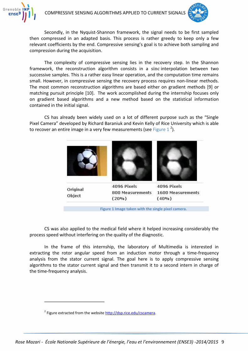
CS has already been widely used on a lot of different purpose such as the “Single Pixel Camera” developed by Richard Baraniuk and Kevin Kelly of Rice University which is able to recover an entire image in a very few measurements (see Figure 1 2).

CS was also applied to the medical field where it helped increasing considerably the process speed without interfering on the quality of the diagnostic.

In the frame of this internship, the laboratory of Multimedia is interested in extracting the rotor angular speed from an induction motor through a time-frequency analysis from the stator current signal. The goal here is to apply compressive sensing algorithms to the stator current signal and then transmit it to a second intern in charge of the time-frequency analysis.

2 Figure extracted from the website http://dsp.rice.edu/cscamera.

Figure 1 Image taken with the single pixel camera.

http://dsp.rice.edu/cscamera



2. General principle of compressive sensing

a) Mathematical representation

Let us denote 𝑥 ∈ ℝn the initial signal, 𝛹 ℝn*n the matrix from the basis in which 𝑥 has the best sparse representation. 𝑋 ∈ ℝn is the best sparse representation from 𝑥 in the basis 𝛹. We then have 𝑥 = 𝛹𝑋.

Let us denote 𝛷 ∈ ℝm*n the sampling matrix allowing to have only 𝑚 measurements from the initial vector 𝑥 and store them in the vector 𝑦 ∈ℝm with 𝑚 ≪ 𝑛.

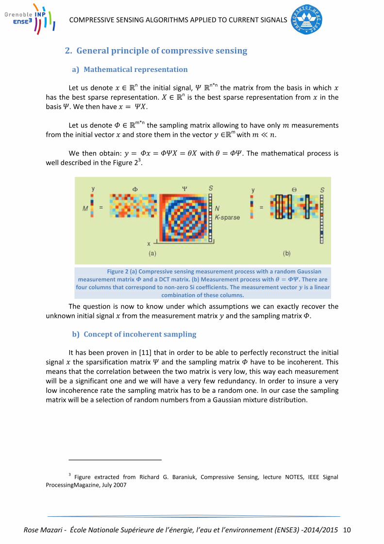
We then obtain: 𝑦 = 𝛷𝑥 = 𝛷𝛹𝑋 = 𝜃𝑋 with 𝜃 = 𝛷𝛹. The mathematical process is well described in the Figure 23.

The question is now to know under which assumptions we can exactly recover the unknown initial signal 𝑥 from the measurement matrix 𝑦 and the sampling matrix 𝛷.

b) Concept of incoherent sampling

It has been proven in [11] that in order to be able to perfectly reconstruct the initial signal 𝑥 the sparsification matrix 𝛹 and the sampling matrix 𝛷 have to be incoherent. This means that the correlation between the two matrix is very low, this way each measurement will be a significant one and we will have a very few redundancy. In order to insure a very low incoherence rate the sampling matrix has to be a random one. In our case the sampling matrix will be a selection of random numbers from a Gaussian mixture distribution.

3 Figure extracted from Richard G. Baraniuk, Compressive Sensing, lecture NOTES, IEEE Signal

ProcessingMagazine, July 2007

Figure 2 (a) Compressive sensing measurement process with a random Gaussian measurement matrix 𝜱 and a DCT matrix. (b) Measurement process with 𝜽 = 𝜱𝜳. There are

four columns that correspond to non-zero Si coefficients. The measurement vector 𝒚 is a linear combination of these columns.



Definition: The coherence between sampling matrix 𝛷 and sparsification matrix 𝛹 is defined by [12] 𝜇(𝛷,𝛹) = √𝑛 × max | <𝛷,𝛹 > | (1)

c) The Restricted Isometry Property

In order to perfectly recover the signal the sampling matrix 𝛷 has to obey to another condition known as the Restricted Isometry Property (R.I.P.).

Definition: [13] A matrix 𝛷 ∈ ℝm*n satisfies the R.I.P. property to the order 𝑘 ∈ ℕ, of isometry constant 𝛿𝑘 ∈ ]0,1[ , if for a signal 𝑥 with 𝑘 non zero coefficients we have:

(1 − 𝛿𝑘)||𝑥||𝑙22 ≤ ||𝛷𝑥||𝑙2

2 ≤ (1 + 𝛿𝑘)||𝑥||𝑙22

(2)

d) Problem Statement

Suppose that we observe:

𝑦 = 𝛷𝑥 (3) Where 𝑥 ∈ℝn is the signal we aim to reconstruct, 𝑦 ∈ℝm is the measurement vector

and 𝛷 is a known 𝑚 × 𝑛 matrix.

Since the number of measurements 𝑚 is a lot smaller than the number of actual samples 𝑛 we have an undetermined case where there are fewer equations than unknowns. If we suppose now that 𝑥 is known to be a sparse signal in a different basis we then have a lot less unknowns parameters since the number of non-zero coefficient is a lot smaller than the number of samples which forms the finite signal 𝑥. This new information makes the problem feasible and offers a new formulation:

𝑚𝑖𝑛∑ |𝑋|0𝑁−1𝑘=0 subject to 𝜃𝑋 = 𝑦 (4)

Where 𝑋 is the sparse representation of 𝑥 and where ||𝑋||0 = ∑ |𝑋|0𝑁−1𝑘=0 is called the

𝑙0 norm.

The issue is that the 𝑙0 norm leads to an NP-hard optimization problem and its

calculation complexity is of order (𝑛𝑘). In theory NP-hard problems can be solved but as the

parameters 𝑛 and 𝑘 increase the processing time increases and the problem becomes unsolvable. This is where the R.I.P. intervenes. Indeed, if the sampling matrix 𝛷 satisfies the restricted isometry property it has been shown in [14] that the 𝑙0 and 𝑙1 problems are in fact equivalent. This way, our problem is now a convex optimization problem whose solution exists and can be find. Other norms 𝑙𝑝 have been tested with 0 < 𝑝 < 1 and a discussion can be found at the beginning of [3].

Our problem has a new formulation:

𝑚𝑖𝑛∑ |𝑋|1𝑁−1𝑘=0 subject to 𝜃𝑋 = 𝑦 (5)



3. Gradient Based reconstruction

The gradient based reconstruction algorithm has been chosen for this application because it doesn’t require to the initial signal to have any specific property except for its sparsity and its compliance to the R.I.P. Plus, the algorithm is easily understandable and easily implemented on MATLAB while being nearly as efficient as most of the reconstruction algorithm. See [14] for a comparison between the different recovery algorithms.

a) Gradient Based Algorithm principle

This algorithm is based on the classical gradient descent algorithm well known in the literature of signal processing methods. The missing samples will be estimated as the ones offering the best concentration measure in the sparse domain. In other words, the missing samples are iteratively changed toward the concentration measure in order to approach the minimum of the 𝑙1-norm based sparsity measure. The concentration of the signal transform 𝑋(𝑘) = 𝑇[𝑥(𝑛)] can be measured by a function close from the 𝑙1 norm and the gradient value will directly result from the concentration measure:

𝑀1[𝑇[𝑥(𝑛)]] =

1

𝑁∑|𝑋(𝑘)|1

𝑘

(6)

In order to find the minimum of a function using the gradient algorithm one takes

iterative steps proportional to the gradient value of the function at the current point. In other words the next value is deduced from the current value minus a certain proportion of the gradient:

𝑦𝑚+1(𝑛) = 𝑦𝑚(𝑛) − 𝜇𝐺(𝑛) (7) With:

𝑦𝑚 ∈ℝn the reconstructed signal at the iteration 𝑚.

𝑦𝑚+1 ∈ℝn the reconstructed signal at the iteration 𝑚 + 1.

𝐺(𝑛) The gradient value applied to each sample.

Once we converge towards the optimal point, ie: towards the minimum of the 𝑙1-norm, the gradient starts oscillating around the solution since the 𝑙1-norm is convex (see Figure 3) everywhere except at the optimal point. The precision of the achieved solution depends strongly from the algorithm’s step. But if we reduce the step from the beginning, the number of iterations needed to achieve a highly accurate solution is considerably huge and the processing time will grow consequently. The solution consists in adapting the step along the iterations. We choose an initial step value and once the gradient starts oscillating around the solution we reduce the step value and allow the gradient algorithm to keep iterating until the next oscillating phase. In order to know when to reduce the algorithm’s step we need to know when the gradient starts oscillating around the optimal point.



Therefore, the measurement of the gradient’s angle 𝛽𝑚 between two successive values 𝑔𝑚−1(𝑛) and 𝑔𝑚(𝑛) is necessary and computed by the following formula extracted from [1]:

𝛽𝑚 = arccos

∑ 𝑔𝑚−1(𝑛) × 𝑔𝑚(𝑛)𝑁−1𝑛=0

√∑ (𝑔𝑚−1(𝑛))²𝑁−1𝑛=0 ×√∑ (𝑔𝑚(𝑛))²

𝑁−1𝑛=0

(8)

The stopping criterion of the algorithm can be either the number of iteration achieved by the algorithm or the value of the step, ie: if the step 𝜇 goes below a fix value ξ the iterations stop and the precision achieved will be the one dictated by the constantξ. A third solution is chosen here. The precision of the result will be estimated from the changes between the recovered signal at the last iteration and the recovered signal at the iteration before that. Therefore the criterion becomes [1]:

𝑇𝑟 = 10𝑙𝑜𝑔10

∑ |𝑦𝑝(𝑛) − 𝑦𝑚(𝑛)|²𝑛∉𝑁𝐴

∑ |𝑦𝑚(𝑛)|²𝑛∉𝑁𝐴

(9)

With:

𝑦𝑚 ∈ℝn the reconstructed signal at the iteration 𝑚.

𝑦𝑝 ∈ℝn the reconstructed signal at the iteration 𝑚 − 1.

If 𝑇𝑟 is below a certain threshold 𝑇𝑚𝑎𝑥 set be the user (in our case 𝑇𝑚𝑎𝑥 ≈ −100𝑑𝐵) the algorithm stops.

The gradient based recovery algorithm can be used in most of the transformation domains as long as the signal to recover is considered sparse in this domain. In our case the gradient based algorithm will be tested on only two transformation domains: the Discrete Fourier Transform (D.F.T.) domain and the Discrete Cosine Transform (D.C.T.) domain. A general and simplified view at the algorithm is given in the next section.

Figure 3 Measure of the l1-norm as a function of missing samples



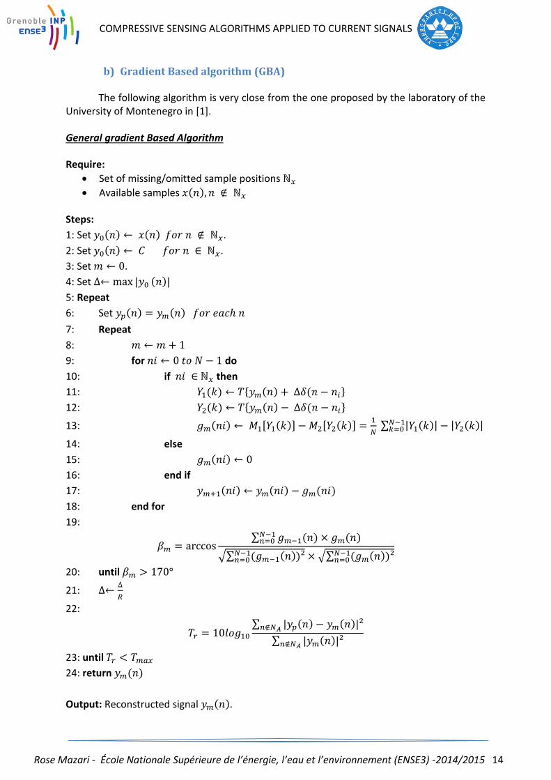
b) Gradient Based algorithm (GBA)

The following algorithm is very close from the one proposed by the laboratory of the University of Montenegro in [1].

General gradient Based Algorithm

Require:

Set of missing/omitted sample positions ℕ𝑥

Available samples 𝑥(𝑛), 𝑛 ∉ ℕ𝑥

Steps:

1: Set 𝑦0(𝑛) ← 𝑥(𝑛) 𝑓𝑜𝑟 𝑛 ∉ ℕ𝑥.

2: Set 𝑦0(𝑛) ← 𝐶 𝑓𝑜𝑟 𝑛 ∈ ℕ𝑥.

3: Set 𝑚 ← 0.

4: Set ∆← max |𝑦0 (𝑛)|

5: Repeat

6: Set 𝑦𝑝(𝑛) = 𝑦𝑚(𝑛) 𝑓𝑜𝑟 𝑒𝑎𝑐ℎ 𝑛

7: Repeat

8: 𝑚 ← 𝑚 + 1

9: for 𝑛𝑖 ← 0 𝑡𝑜 𝑁 − 1 do

10: if 𝑛𝑖 ∈ ℕ𝑥 then

11: 𝑌1(𝑘) ← 𝑇{𝑦𝑚(𝑛) + ∆𝛿(𝑛 − 𝑛𝑖}

12: 𝑌2(𝑘) ← 𝑇{𝑦𝑚(𝑛) − ∆𝛿(𝑛 − 𝑛𝑖}

13: 𝑔𝑚(𝑛𝑖) ← 𝑀1[𝑌1(𝑘)] − 𝑀2[𝑌2(𝑘)] =1

𝑁 ∑ |𝑌1(𝑘)| − |𝑌2(𝑘)|𝑁−1𝑘=0

14: else

15: 𝑔𝑚(𝑛𝑖) ← 0

16: end if

17: 𝑦𝑚+1(𝑛𝑖) ← 𝑦𝑚(𝑛𝑖) − 𝑔𝑚(𝑛𝑖)

18: end for

19:

𝛽𝑚 = arccos∑ 𝑔𝑚−1(𝑛) × 𝑔𝑚(𝑛)𝑁−1𝑛=0

√∑ (𝑔𝑚−1(𝑛))²𝑁−1𝑛=0 ×√∑ (𝑔𝑚(𝑛))²

𝑁−1𝑛=0

20: until 𝛽𝑚 > 170°

21: ∆←∆

𝑅

22:

𝑇𝑟 = 10𝑙𝑜𝑔10∑ |𝑦𝑝(𝑛) − 𝑦𝑚(𝑛)|²𝑛∉𝑁𝐴

∑ |𝑦𝑚(𝑛)|²𝑛∉𝑁𝐴

23: until 𝑇𝑟 < 𝑇𝑚𝑎𝑥

24: return 𝑦𝑚(𝑛)

Output: Reconstructed signal 𝑦𝑚(𝑛).



Comments on the General gradient Based Algorithm

Steps:

2: The non-available samples are put to the value of the constant 𝐶. This constant is often

set to zero, although it can be changed into the average value of the available samples. A

descent algorithm where the initial value is set too far from its real value can easily diverge.

4: Same thing than for the second step. The Algorithm step ∆ is set to the maximum value of

the available sample but it can be set to other values if the algorithm doesn’t seem to

converge.

6-20: For each sample of the vector with missing sample we compute a gradient value

depending on the step value ∆ and the concentration value. If the sample is available the

gradient value is considered null.

For each iteration we compute the gradient’s angle between the last two values. If the angle

exceeds 170° the algorithm’s step is reduced. The constant 𝑅 is often such as 𝑅 = √10

which offers a good compromise between the program’s running speed and the level of

accuracy achieved.

22-24: If the stopping criterion 𝑇𝑟 has been reached the signal at the iteration 𝑚 is

considered as the reconstructed signal. If the initial signal is available (our case) we can add a

step to measure the reconstruction error.

One simple algorithm can be found in the ANNEX A MATLAB CODE OF THE GBA

Now that the theory has been explored in details the next section focuses on the results of the algorithm on different type of signals, the stator current signal included.



4. Gradient Based algorithm results

a) Sinus reconstruction using the gradient based algorithm

The signal

The GBA is applied to a sinusoidal signal of length 256 both in the DFT and DCT

domain. The signal is as follow: 𝑥(𝑛) = 2 × sin (20 × 𝜋 ×𝑛

𝑁).

95% of the samples are going to be removed. The goal is to be able to perfectly reconstruct the sinusoidal signal sparse in both DFT and DCT domains.

Figure 4 Original Signal

Figure 5 Original signal with 95% missing sample



GBA in the DFT domain

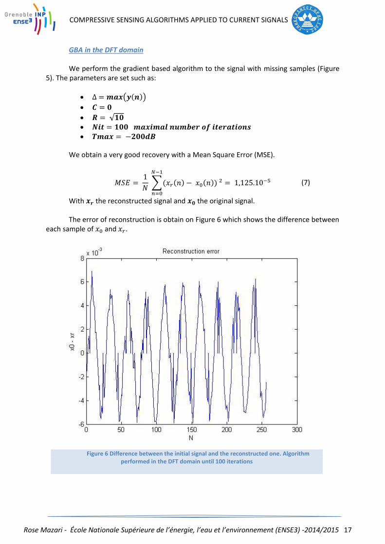
We perform the gradient based algorithm to the signal with missing samples (Figure 5). The parameters are set such as:

∆ = 𝒎𝒂𝒙(𝒚(𝒏))

𝑪 = 𝟎

𝑹 = √𝟏𝟎 𝑵𝒊𝒕 = 𝟏𝟎𝟎 𝒎𝒂𝒙𝒊𝒎𝒂𝒍 𝒏𝒖𝒎𝒃𝒆𝒓 𝒐𝒇 𝒊𝒕𝒆𝒓𝒂𝒕𝒊𝒐𝒏𝒔 𝑻𝒎𝒂𝒙 = −𝟐𝟎𝟎𝒅𝑩

We obtain a very good recovery with a Mean Square Error (MSE).

𝑀𝑆𝐸 = 1

𝑁 ∑(𝑥𝑟(𝑛) − 𝑥0(𝑛))

2 = 1,125.10−5𝑁−1

𝑛=0

(7)

With 𝒙𝒓 the reconstructed signal and 𝒙𝟎 the original signal.

The error of reconstruction is obtain on Figure 6 which shows the difference between each sample of 𝑥0 and 𝑥𝑟.

Figure 6 Difference between the initial signal and the reconstructed one. Algorithm performed in the DFT domain until 100 iterations



GBA in the DCT domain

We now perform the exact same algorithm with the same initial signal and the same parameters in the DCT domain. The error is higher 𝑴𝑺𝑬 = 𝟏, 𝟓𝟓𝟑𝟐 and the computational time is longer.

DFT and DCT comparison

Since the noise created by the missing samples is greater in the DCT domain than in the DFT domain, it is harder to minimize the concentration and therefore achieving better results in the DCT domain. The GBA applied in the DFT domain shows better performances than in the DCT domain when applied to a finite sinusoidal signal. It has better running speed while reaching a lower MSE. For theses reason this domain will be preferred for the compression of the stator current.

DFT DOMAIN DCT DOMAIN Elapsed time ΔT (s) 𝟏, 𝟏𝟏𝟐 𝟐, 𝟑𝟓𝟕 Mean Square Error 𝟏, 𝟏𝟐𝟓𝟏𝟎−𝟓 𝟏, 𝟓𝟓𝟑𝟐

Figure 8 Comparison between DFT & DCT sparse domain

Figure 7 Difference between the original signal and the reconstructed one algorithm performed in the DCT domain until 100 iterations



We can still improve the performances of the algorithm by dividing the running time and increase the convergence sped. The processing time can be reduced by obliging the MATLAB Fourier transform to be computed on a length corresponding to a power of two.

We can also play on the parameter Δ. It is a good way to increase the precision without adding new iterations. We need to increase the initial Δ value, this way we avoid several iterations we could have had if the step was too small. But we do not want the Δ to be too high for two reasons. First the algorithm could diverge; second, if the initial step is set too high and not reduced enough during the iterations, the algorithm might end with a very low precision. A good combination would be to increase the initial Δ and reduce it quickly iterations after iterations in order to reach a better precision by the end of the iterations.

We might also set the missing sample at the average value of the overall signal in order to converge more quickly.

We chose new parameters for the algorithm and applied it to the same sinus signal. The results are shown in the Figure 9 and Figure 10:

∆ = 𝟑 ×𝒎𝒂𝒙(𝒚(𝒏))

𝑪 = 𝒎𝒆𝒂𝒏(𝒚(𝒏)) 𝑹 = 𝟓 𝑵𝒊𝒕 = 𝟏𝟎𝟎 𝒎𝒂𝒙𝒊𝒎𝒂𝒍 𝒏𝒖𝒎𝒃𝒆𝒓 𝒐𝒇 𝒊𝒕𝒆𝒓𝒂𝒕𝒊𝒐𝒏𝒔 𝑻𝒎𝒂𝒙 = −𝟐𝟎𝟎𝒅𝑩

Δ = max(y(n))

Δ = 3 *max(y(n))

Elapsed time ΔT (s) 𝟏, 𝟏𝟏𝟐 𝟏, 𝟏𝟏𝟎𝟖 Mean Square Error 𝟏, 𝟏𝟐𝟓𝟏𝟎−𝟓 𝟑, 𝟕𝟐𝟒𝟏𝟎−𝟔

(a) (b)

Figure 9 Algorithm Improvement

Figure 10 Evolution of Beta for (a) Δ = max(y(n)) and (b) Δ =3* max(y(n))



b) Gradient Based algorithm applied to the stator current

The main goal of the other intern is to extract the rotor angular speed from a time frequency analysis of the stator current. As precised in the introduction our goal here is to be able to greatly compress this stator current signal without losing the information allowing to extract the rotor angular speed

The rotor angular speed may be estimated by only measuring and analyzing the stator current and its harmonics, if these harmonics exist. These latter harmonics, called Rotor Slot Harmonics (RSH), are proved to be directly proportional to the rotor speed. By using Time -Frequency analysis, the RSHs may be extracted from the current signal, giving the evolution of the rotor speed over the time.

The stator current signal is obtained from a realistic model of induction motor. This model takes into account the dynamic behavior of the machine by coupling mechanic and electromagnetism models. This enables to simulate harmonics and noises in the stator current, which features the RSHs. On the Figure 11 we can see the initial signal and its Fourier transform displayed on a logarithmic scale. Both are 16 800 samples long.

(a) (b)

We can notice on the Figure 11 (b) that the current signal is not sparse in the DFT domain. We therefore need to make it sparse in order to be able to recover it perfectly. The RSH component varies in the range [0Hz-700Hz].

The easiest method to sparsify the signal while keeping the RSH component is:

Since the RSH evolves from 0HZ-800Hz we put to zero every frequency above

800Hz.

Figure 11 (a) Stator current IaJ03 label axis=sample (b) Stator current Fourier transform on a logarithmic scale



Threshold the spectrum of the initial current signal and put to zero every

coefficient below the threshold.

The chosen threshold is of 30 since the amplitude of RSH doesn’t go below this value during the time interval. With theses parameters the percentage of non-zero coefficients in the DFT domain is of K = 8% we can consider the signal as sparse in this domain.

By computing the inverse DFT we obtain the sparse initial signal on which we apply

the GBA in the DFT domain after removing 75% of the samples. We obtain rather good results with this method and we are able to extract the RSH component to approximate the rotor angular speed. Nevertheless, this method has two major disadvantages. Because we need to sparsify the signal and to know its properties in order to sparsify it. This method might be better used in a transmitting process rather than an acquiring one.

Figure 12 Logarithmic DFT of the stator current Figure 13 Logarithmic DFT of the stator current after spasification

Figure 14 Reconstruction error between the original signal x0 and the recovered one xr

Figure 15 in blue the extracted RSH component from the recovered current signal- In green the theoritical speed



c) Extension of the GBA to the images

Until now we considered only signals that had no spatial properties. We are going to apply the GBA to an image pre- sparsified in the DCT domain. It is not the main goal of the internship but it is rather interesting to see the results. The initial image contains rather low frequencies in order to suppress very few information by sparsifying in the DCT domain. The algorithm is performed on successive 8 𝑏𝑦 8 blocks for each Red, Green, Blue bands and the missing sample rate is of 75%. The image being sparsified in the DCT domain the result is more efficient in this domain

Figure 16 GBA performed on a low frequency image in the DFT domain

Figure 17 GBA performed on a low frequency image in the DCT domain



5. General Deviation algorithm

The General Deviation algorithm is different from the large majority of recovery algorithms. This algorithm is not greedy in time since it does not require any iterative process and the recovery is based on the statistics information of the signal. It links both signal estimation theory and compressive sensing. The frequency domain (DFT) is the chosen sparsity domain although the same principles can be applied to other domains as long as the initial signal is sparse.

Several samples are going to be removed from the initial signal. As a result, the signal is no longer sparse in the transformation domain. By calculating the sum of the general deviation on the signal with missing sample we can distinguish the signal’s components from the noise. We apply a threshold to select the components and rebuild the original signal. If a component was “hidden” by the noise and could not be selected by the threshold, we need to apply the algorithm on more time to the signal from which the previously detected components have been removed.

a) General Deviation principles

We consider a signal as a sum of 𝐾 sinusoidal components in the form:

𝑥(𝑛) =∑𝐴𝑖exp (

𝑗2𝜋𝑘0𝑖𝑛

𝑁+ 𝜑𝑖)

𝐾

𝑖=1

(10)

Where 𝑘0𝑖 denotes the 𝑖-th signal frequency while 𝐴𝑖 and 𝜑𝑖 denote the amplitude and phase of the 𝑖-th component. The signal is 𝐾-sparse in the DFT domain.

The compressive sensing problem statement remains the same as earlier in (5).

Estimation Basic theory

We consider the signal 𝑥(𝑛) to which we add a noise 𝑏(𝑛).

𝐴(𝑛) = 𝑥(𝑛) + 𝑏(𝑛) (11) The goal here is to be able to estimate the signal’s transform 𝑋(𝑘) . The estimated

coefficient will be denoted �̂�(𝑘). In order to solve this problem, on approach consists in minimizing the total error [15]:

𝐼 = ∑ 𝐹 {|𝑥(𝑛)𝑒𝑥𝑝−

𝑗2𝜋𝑘𝑛𝑁 − 𝑋(𝑘)|}

𝑁−1

𝑛=0

(12)

Where 𝐹{ } is a loss function corresponding to a certain norm. For the 𝑙2-norm, 𝐹{𝑒(𝑛)} = |𝑒|² and for the 𝑙1-norm we have 𝐹{𝑒(𝑛)} = |𝑒|. Within the loss function’s brackets we have the error function.

𝑒(𝑛𝑚,, 𝑘) = |𝑥(𝑛)𝑒𝑥𝑝

−𝑗2𝜋𝑘𝑛𝑁 − 𝑋(𝑘)| (13)

Where 𝑚 is the number of available samples.



The minimum of (12) can be obtained from:

𝑑𝐼

𝑑𝑋= 0 (14)

The solution obtained by solving (12)-(14) is called the 𝑀-estimate. In other words we obtain a model of estimation. If the loss function is such as 𝐹{𝑒(𝑛)} = |𝑒|² we then have the classical discrete transform:

𝐴(𝑘) = �̂�(𝑘) = 𝑚𝑒𝑎𝑛⏟

𝑛𝑚∈ℕ𝑎𝑣𝑎𝑖𝑙𝑎𝑏𝑙𝑒

{𝑥(𝑛1)𝑒−𝑗2𝜋𝑘𝑛1

𝑁 , … , 𝑥(𝑛𝑚)𝑒−𝑗2𝜋𝑘𝑛𝑚

𝑁 } (15)

This solution has very nice estimation properties if the noise 𝑏(𝑛) is a Gaussian noise. It has been proven that (15) is the Maximum of Likelihood (M.L.), in other words: there is no better estimate of 𝑋(𝑘) than the one described in (15) if the noise is Gaussian. Nonetheless, the Maximum of Likelihood is rather sensitive to the changes in the noise’s probability density function (p.d.f.) and shows to be a lot less efficient as soon as the noise is not a Gaussian one. The function loss according to the 𝑙1-norm appears to be more robust to pdf changes and particularly on the worse kind of noise: the Laplacian noise (impulse). Although being less efficient on a Gaussian noise, it will insure a good estimation on the large majority of cases. With the loss function such as 𝐹{𝑒(𝑛)} = |𝑒| we obtain the following estimation [16]:

𝐴(𝑘) = �̂�(𝑘) = 𝑚𝑒𝑑𝑖𝑎𝑛⏟

𝑛𝑚∈ℕ𝑎𝑣𝑎𝑖𝑙𝑎𝑏𝑙𝑒

{𝑅𝑒 {𝑥(𝑛1)𝑒−𝑗2𝜋𝑘𝑛1


𝑁 }}

+ 𝑗 𝑚𝑒𝑑𝑖𝑎𝑛⏟ 𝑛𝑚∈ℕ𝑎𝑣𝑎𝑖𝑙𝑎𝑏𝑙𝑒

{𝐼𝑚 {𝑥(𝑛1)𝑒−𝑗2𝜋𝑘𝑛1


𝑁 }} (16)

General Deviation Computation

After having the error values for each available sample we compute the sum of the general deviation for each frequency 𝒌 ∈ [𝟏,𝑵].

𝐺𝐷(𝑘) =

1

𝑀 ∑ 𝐹{| 𝑒(𝑛𝑖, 𝑘) − 𝑚𝑒𝑎𝑛(𝑒(𝑛1, 𝑘), … , 𝑒(𝑛𝑚, 𝑘)|}

𝑛𝑖 ∈ℕ𝑎𝑣𝑎𝑖𝑙𝑎𝑏𝑙𝑒

(17)

The algorithm is rather flexible because it allows choosing between the two norms in

order to improve the estimation. If it is an 𝒍𝟐-norm, the general deviation can be considered as a variance value.



Variance of noise

It has been proven in [17] (see

ANNEX B for details) that the variance of spectral noise caused by missing sample is:

𝜎²𝑖 ∉ℕ𝑎𝑣𝑎𝑖𝑙𝑎𝑏𝑙𝑒 = 𝑀

𝑁 −𝑀

𝑁 − 1∑𝐴²𝑖

𝐾

𝑖=1

(18)

Where 𝑴is the number of available samples, 𝑵 is the signal’s length and 𝑨𝒊 the amplitude of the 𝒊-th non available sample.

The general deviation of the signal components will always be below the limit expressed in (18), therefore we can express the following empirical threshold to detect the components’s frequencies:

𝑇 = 𝛼 × max (𝐺𝐷(𝑘)) (19) Where 𝑻 is the threshold and 𝜶 a coefficient often included in [0.8, 0.95].

𝐿 = 𝑎𝑟𝑔𝑚𝑖𝑛{𝐺𝐷(𝑘) < 𝑇} (20) Where 𝑳 is a vector containing the frequencies below the threshold and in most

cases these are the components’s frequencies.



b) General Deviation Algorithm

General Deviation Algorithm 1

Require:

Set of missing/omitted sample positions ℕ𝑥

Available samples 𝑥(𝑛), 𝑛 ∉ ℕ𝑥

Steps:

1: Set 𝑦(𝑛) ← 𝑥(𝑛) 𝑓𝑜𝑟 𝑛 ∉ ℕ𝑥.

2: Set 𝑦(𝑛) ← 𝐶 𝑓𝑜𝑟 𝑛 ∈ ℕ𝑥.

3: Set 𝛼 ∈ [0,1]

4: Set 𝑁𝑜𝑟𝑚 𝑡𝑜 1 𝑜𝑟 2

5: For 𝑘 ← 0 to 𝑁 do

6: For 𝑛 ← 0 to 𝑀do

7: 𝑇(𝑘, 𝑛) = 𝑦(1, 𝑛)𝑒𝑥𝑝−𝑗2𝜋𝑘𝑛

𝑁 𝑓𝑜𝑟 𝑒𝑎𝑐ℎ 𝑛 ∉ ℕ𝑥 𝑎𝑛𝑑 𝑓𝑜𝑟 𝑒𝑎𝑐ℎ 𝑘 ∈ ℝ𝑁

8: end for

9: if 𝑁𝑜𝑟𝑚 = 2 then

10: 𝐺𝐷(𝑘) = 1

𝑀 ∑ |𝑒(𝑛𝑖, 𝑘) − 𝑚𝑒𝑎𝑛(𝑒(𝑛1, 𝑘),… , 𝑒(𝑛𝑚, 𝑘)|𝑛𝑖 ∈ℕ𝑎𝑣𝑎𝑖𝑙𝑎𝑏𝑙𝑒

²

11: else

12: 𝐺𝐷(𝑘) = 1


13: end if

14: End for

15: 𝑇 = 𝛼 × max (𝐺𝐷(𝑘))

16: 𝐿 = 𝑎𝑟𝑔𝑚𝑖𝑛{𝐺𝐷(𝑘) < 𝑇}

17: 𝐼𝐷𝐹𝑇 = 𝑑𝑓𝑡𝑚𝑡𝑥(𝑁)

18: 𝜃 = 𝐼𝐷𝐹𝑇(𝑛, 𝐿) 𝑓𝑜𝑟 𝑛 ∉ ℕ𝑥

19: 𝜃−1 × 𝑦(𝑛) = �̂�(𝑘)

20: �̂�(𝑘) = (𝜃𝑇𝜃)−1𝜃𝑇𝑦

21: �̂�(𝑛) = ∫ �̂�(𝑘)𝑒𝑥𝑝−𝑗2𝜋𝑘𝑛

𝑁 𝑑𝑘∞

−∞



Comments on the General Deviation Algorithm

Steps

3: The parameter 𝛼 sets the threshold value

4: Be default the 𝑁𝑜𝑟𝑚 is set to 1 but if we know the noise is Gaussian the norm is set to 2.

17: 𝐼𝐷𝐹𝑇 is an 𝑛 by 𝑛 matrix whose product with a vector computes the Fourier Transform of the vector.

18: 𝜃 is now an 𝑛 by 𝐿 matrix. With 𝑛 ∉ ℕ𝑥 being the number of measured samples and 𝐿 a vector containing the frequency components being below the threshold. The product of 𝜃 with another vector produces the Fourier transform of the vector.

19: By doing this operation we can reconstruct the Fourier Transform of the estimated initial signal. Problem: 𝜃 is not invertible.

20: Solution: since 𝜃𝑇𝜃 is invertible, we perform the Moore-Penrose pseudoinverse operation on the matrix 𝜃. Property of the Moore-penrose inverse:

𝐴−1 = (𝐴𝑇𝐴)−1𝐴𝑇 (21) 21: By computing the inverse transform from the estimated Fourier signal we obtain an estimation of the initial signal in time.



6. Results of the General Deviation Algorithm

a) Theoretical framework

We consider a signal as a sum of 𝐾 sinusoidal components in the form:

𝑥(𝑛) =∑𝐴𝑖exp (

𝑗2𝜋𝑘0𝑖𝑛

𝑁)

𝐾

𝑖=1

()

Where 𝑘0𝑖 denotes the 𝑖-th signal frequency while 𝐴𝑖 denote the amplitude of the 𝑖-th component. The signal is 𝐾-sparse in the DFT domain and is 128 points long both in time and frequency domains.

b) First example

In the first example we want to show a simple application of the proposed algorithm. Thus we consider a signal with only three components and with very close amplitudes:

𝑥(𝑛) = 𝐴1𝑒𝑥𝑝

−𝑗2𝜋𝑓1𝑛𝑁 + 𝐴2𝑒𝑥𝑝

−𝑗2𝜋𝑓2𝑛𝑁 + 𝐴3𝑒𝑥𝑝

−𝑗2𝜋𝑓3𝑛𝑁 ()

With A = [1.1, 1, 0.95] and f = [16, 32, 64].

Figure 18 (a) Original signal x(n). (b) Original signal with a Gaussian noise with sigma = 0 and average = 0. (c) Original signal with 85% of removed samples. (d) Recovery of the initial signal.



There is no addition of noise to the original signal since the parameters 𝜎 and 𝑚 are set to zero. On the Figure 18 (c), 85% of samples are being removed. And after computing the general deviation we apply a threshold with an 𝛼 of 0,85. Since there is no noise the general deviation is computed with a function loss such as: 𝐹{𝑒} = |𝑒|².

The threshold is set so we select only three frequencies components: the 16 𝐻𝑧, the 32𝐻𝑧 and the 64𝐻𝑧. The initial signal is almost perfectly reconstruct except for an amplitude problem which is due to the uniqueness of the θ matrix which doesn’t emphasize the amplitude of each component. This problem can be easily overruled by calculating the amplitude value of each frequency component by using equation (15) or (16) depending on the norm.

Figure 19 General Deviation computation for an L2 Norm



c) Second example

In this example a small noise is added to the initial signal to test the algorithm’s robustness and to see the effect of the norm on the reconstruction.

Gaussian noise

The first noise that we add to the signal is a Gaussian noise of variance 𝝈 = 𝟎, 𝟓 and mean 𝒎 = 𝟎. The function loss follows an 𝒍𝟐-norm and is such as: 𝐹{𝑒} = |𝑒|². As previously explained the 𝒍𝟐-norm is netter equipped to cope with the Gaussian noise pfd. Therefore the recovery results will be better than with an 𝒍𝟏-norm. See Figure 20(d) and 21(d) for a comparison of the initial signal reconstruction.

Figure 20 (a) Original signal x(n). (b) Original signal with a Gaussian noise with sigma = 0,5 and average = 0. (c) Original signal with 85% of removed samples. (d) Recovery of the initial signal with an l2 norm.

Figure 21 (a) Original signal x(n). (b) Original signal with a Gaussian noise with sigma = 0,5 and average = 0. (c) Original signal with 85% of removed samples. (d) Recovery of the initial signal with an l1 norm.



Impulse noise

The second noise that we add to the signal is an impulsion noise composed of three peaks with an amplitude that varies between 10 and 11 when the signal’s component do not go high than 1.1. The function loss follows an 𝒍𝟐-norm and is such as: 𝐹{𝑒} = |𝑒|². As previously explained the 𝒍𝟏-norm is better equipped to cope with the impulse noise pfd. Therefore the recovery results will be better than with an 𝒍𝟐-norm. See Figure 22(d) and 23(d) for a comparison of the initial signal reconstruction.

Figure 22 (a) Original signal x(n). (b) Original signal with 3 impulsion noise. (c) Original signal with 85% of removed samples. (d) Recovery of the initial signal with an l1 norm.

Figure 23 (a) Original signal x(n). (b) Original signal with 3 impulsion noise. (c) Original signal with 85% of removed samples. (d) Recovery of the initial signal with an l2 norm.



d) General deviation algorithm applied to the stator current

We apply the GDA algorithm to the stator current in Figure 11(a). Since we don’t know the type of noise created by the induction machine, the algorithm is performed with a loss function such as: 𝐹{𝑒} = |𝑒| following the 𝑙1-norm. The parameter 𝛼 is set to 𝛼 = 0,85. On Figure 24(a) and (b) we can see that the threshold was too rough to be able to select all the components we needed. Plus, even if we could set it in order to get the right components we might collect a lot of undesired frequencies (b).

(a) (b)

The stator current is a more complex signal than the one taken for the examples

above. Indeed, this signal has a lot of components with different amplitudes which makes harder the selection of the components by one threshold only. The solution might be to implement an iterative solution.

Figure 24 (a) Threshold (in red) on the stator current's General Deviation (b) Zooming on the selected components



General gradient Based Algorithm 2

Same requirements than before. Steps:

1: Set 𝑦(𝑛) ← 𝑥(𝑛) 𝑓𝑜𝑟 𝑛 ∉ ℕ𝑥.

2: Set 𝑦(𝑛) ← 𝐶 𝑓𝑜𝑟 𝑛 ∈ ℕ𝑥.

3: Set 𝛼 ∈ [0,1]

4: Set 𝑁𝑜𝑟𝑚 𝑡𝑜 1 𝑜𝑟 2

5: 𝑚 = 0

6: For 𝑐 ← 1 to 𝑃 do

7: 𝑚 ← 𝑚 + 1

8: For 𝑘 ← 0 to 𝑁 do

9: For 𝑛 ← 0 to 𝑀do

10: 𝑇(𝑘, 𝑛) = 𝑦𝑚(1, 𝑛)𝑒𝑥𝑝−𝑗2𝜋𝑘𝑛

𝑁 𝑓𝑜𝑟 𝑒𝑎𝑐ℎ 𝑛 ∉ ℕ𝑥 𝑎𝑛𝑑 𝑓𝑜𝑟 𝑒𝑎𝑐ℎ 𝑘 ∈ ℝ𝑁

11: end for


13: 𝐺𝐷(𝑘) = 1


²

14: else

15: 𝐺𝐷(𝑘) = 1


16: end if

17: End for

18: 𝑘 = min(𝐺𝐷(𝑘))𝑤𝑖ℎ 𝑘 ∈ ℝ𝑃


19: �̂�(𝑘) = 𝑚𝑒𝑎𝑛⏟ 𝑛𝑚∈ℕ𝑎𝑣𝑎𝑖𝑙𝑎𝑏𝑙𝑒

{𝑥(𝑛1)𝑒−𝑗2𝜋𝑘𝑛1


𝑁 }

20: Else if 𝑁𝑜𝑟𝑚 = 1 then

21: �̂�(𝑘) = 𝑚𝑒𝑑𝑖𝑎𝑛⏟ 𝑛𝑚∈ℕ𝑎𝑣𝑎𝑖𝑙𝑎𝑏𝑙𝑒

{𝑅𝑒 {𝑥(𝑛1)𝑒−𝑗2𝜋𝑘𝑛1


𝑁 }} +

𝑗 𝑚𝑒𝑑𝑖𝑎𝑛⏟ 𝑛𝑚∈ℕ𝑎𝑣𝑎𝑖𝑙𝑎𝑏𝑙𝑒

{𝐼𝑚 {𝑥(𝑛1)𝑒−𝑗2𝜋𝑘𝑛1


𝑁 }}

22: End if



23: 𝑦𝑚+1(𝑛) = 𝑦𝑚(𝑛) − �̂�(𝑘)𝑒𝑥𝑝−𝑗2𝜋𝑘𝑛

𝑁

24: End for

25: 𝜃 = 𝐼𝐷𝐹𝑇(𝑛, 𝑘) 𝑓𝑜𝑟 𝑛 ∉ ℕ𝑥

26: 𝜃−1 × 𝑦(𝑛) = �̂�(𝑘)

27: �̂�(𝑘) = (𝜃𝑇𝜃)−1𝜃𝑇𝑦

28: �̂�(𝑛) = ∫ �̂�(𝑘)𝑒𝑥𝑝−𝑗2𝜋𝑘𝑛

𝑁 𝑑𝑘∞

−∞

Comments on the General Deviation Algorithm 2

This algorithm will perform better results because it will not cut off the components we need because of a bad threshold setting. Therefore if the noise is not too important, the recovery of the stator current without losing the RSH component can be achieved.

Nevertheless, this algorithm has two disadvantages. First, we need to know the number of components to select before running the algorithm; therefore it cannot be applied to an unknown signal. Second, even if we perform good results with this algorithm, the running time is too long because of the signal’s length and because of the number of iterations. One way to reduce the number of iteration would be to apply several thresholds that select a “group” of components that we remove from the initial signal to apply a new threshold at a new iteration. The total number of iteration is then divided by the mean number of components selected by each threshold.

By lack of time this improved algorithm was not tested on the stator current.



CONCLUSION

Compressive sensing is a recent field in the community of signal processing. A wide range of algorithms have been implemented and we chose to focus on two particular types within the framework of the internship. The first algorithm is based on the computation of the signal’s gradient calculated from the concentration measurements in the transform domain. Although it is an iterative method, the algorithm allowed a fast recovering of the stator signal. The second algorithm is based on the statistical properties of the signal and computes the sum of general deviation. The first implementation was a non-iterative one and did not allow recovering the entire signal although it has great performances on reconstructing signals whose components have similar amplitude. Therefore, another algorithm was done and this time including an iterative procedure. Time was too short to implement and test the algorithm but it will most likely give efficient results even with the increase of the running time.

More than a strictly technical achievement, we also enjoyed a new working method where we were able to manage our schedule and work in autonomy. The Laboratory of Multimedia provided us with a great working environment and our tutor and colleagues were happy to share their knowledge every time we had a question.

This internship at the University of Montenegro gave us the opportunity to discover a totally different country filled with a History still unknown for the majority of Western Europeans. Balkans country offers a wide range of beautiful landscapes and beautiful people. I will never forget the heat of Podgorica, the charm of Ada Bojana, the authenticity of the Njegošev mauzolej and the taste of Kačamak.

This internship has been the best experience of my engineering studies and there is no better way to begin an active life.

https://hr.wikipedia.org/wiki/Mauzolej



Bibliography

[1]. Reconstruction of Randomly Sampled Sparse Signals Using Adaptive Gradient Algorithm. Ljubisa Stankovic, Milos Dakovic. Podgorica : s.n., 2014.

[2]. An automated signal reconstruction method based on analysis of compressive sensed signals in noisy environment. Srdjan Stankovic, Irena Orovic, and Ljubisa Stankovic. Podgorica : s.n., 2014.

[3]. Adaptive Variable Step Algorithm for Missing Samples Recovery in Sparse Signals. Ljubisa Stankovic, Milos Dakovic, Stefan Vujovic. Podgorica : s.n., 2013.

[4]. A Relationship between the Robust Statistics Theory and Sparse Compressive Sensed Signals Reconstruction. Srdjan Stankovic, Ljubisa Stankovic, Irena Orovic. Podgorica : s.n., 2013.

[5]. Communication in the Presence of Noise. Shannon, Clause E. Jan 1949.

[6]. Certain topics in telegraph transmission theory. Nyquist, Harry. 1928.

[7]. Compressed sensing. Donoho, D.L. s.l. : Information Theory, IEEE Transactions on, vol 52, no. 4, pp. 1289-1306., 2006.

[8]. Stable signal recovery from incomplete and inaccurate. E. Candès, J. Romberg, and T. Tao. s.l. : Comm. Pure Appl. Math., 59(8):1207-1223, 2006.

[9]. Gradient projection for sparse reconstruction: Application to compressed sensing and other inverse problems. M. A. Figueiredo, R. D. Nowak, and S. J. Wrigh. s.l. : IEEE Journal of Selected Topics in Signal Processing vol. 1, no. 4, pp.586–597, 2007.

[10]. Matching pursuits with time-frequency dictionary. Zhang, S. G. Mallat and Z. s.l. : Signal Processing, IEEE Transactions on vol. 41, no. 12, pp. 3397–3415, 1993.

[11]. Uncertainty principles and ideal atomic decomposition. X.Huo, D.L. Donoho and. s.l. : IEEE Trans. Inform. Theory, vol 47 no 7 pp 2845-2862, Nov 2001.

[12]. Compressive Sensing : « When sparsity meets sampling ». Vandergheynst, Laurant Jacques and Pierre. February 17, 2010.

[13]. The Restricted Isometry Property and its implication for Compressive sensing. Candès, Emmanuel J. s.l. : Applied & Computational Mathematics, California Institute of Technology, Pasadena, CA 91125-5000, 27 Fev 2008.

[14]. Performance Comparisons of Greedy Algorithms in Compressed Sensing. Tanner, Jeffrey D. Blanchard and Jared. Jan 2014.

[15]. Robust Regression: Asymptotics, Conjectures and Monte Carlo. J.Huber, Peter. 1973.



[16]. Robust L-Estimation Based Forms of Signal Transforms and Time-Frequency Representations. Igor Djurovic, LJubisa Stankovic,and Johann F. Böhme. 7.JUly 2003.

[17].An Automated Signal Reconstruction Method based on analysis of Compressive Sensed Signals in Noisy Environnement. Srdjan Stankovic, Irena Orovic and Ljubisa Stankovic. 2014.



ANNEX A MATLAB CODE OF THE GBA

%%%%%%%%%%%%%%%%%%%%%%%%%%%%%%%%%%%%%%%%%% % CS- Adaptative Gradient Algorithm % % Rose Mazari % % 21.04.2015 % %%%%%%%%%%%%%%%%%%%%%%%%%%%%%%%%%%%%%%%%%% clear all, close all, clc

%% Initialisation signals

tic fe = 10; % Sampling frequency N = 256; % Number of samples Miss_pr = 95; % percent nb_miss_samp = round((Miss_pr/100)*N); % Number of missing samples M = N-nb_miss_samp; % Number of available samples

n = 0:N-1; x=2*sin(20*pi*n/N); x0 = x;

%Number max of iteration Iter = 300;

% Generation of the index of missing samples NI=randperm(N); ni=NI(M+1:end); % Available samples na=NI(1:M);

% y signal with missing sample y=x; y(ni)=0;

% Gradient step Delta=max(abs(y)); % Max precision (dB) Tmax = -200;

% % Spasity check % ffty = abs(fft(y)); % F = 1:N/2; % figure;plot(F,ffty(1:N/2));title('DFT of the sinusoidal signal with

50% missing samples f0 = 20Hz');xlabel(' Frequency

samples');ylabel('Amplitude'); % dcty = abs(dct(y)); % F = 1:N/2; % figure;plot(F,dcty(1:N/2));title('DCT of the sinusoidal signal with

50% missing samples f0 = 20Hz');xlabel(' Frequency

samples');ylabel('Amplitude'); % %Gradient algorithm [xr Betam Tr MSE] = grad_fft(y,ni,Delta,Iter,Tmax,x0);



limitBetam = ones(1,length(Betam)).*170; figure; plot(Betam); title('Gradient angle evolution'); xlabel(

'Iterations'); ylabel( 'Beta (°)'); hold on; plot(limitBetam,'r');

limitTr = ones(1,length(Tr)).*Tmax; figure; plot(Tr); title('Precison evolution');xlabel(

'Iterations');ylabel(' Precision (dB)'); hold on; plot(limitTr,'r');

% Display Results figure;subplot(211) stem(abs(fftshift(fft(x0)))) title('Original')

subplot(212) stem(abs(fftshift(fft(xr)))), title('Reconstructed') % length(ni)

recerr=x0-xr; save('recerr.mat') figure plot(recerr); title('Reconstruction error'); xlabel('N');ylabel('x0 - xr'); MSE toc

---------------------------------------------------------------------------------------------------------------------------- function [xr Betam Tr MSE] = grad_fft(x,ni,Delta,Iter,Tmax,x0) y = x; N = length(y); nb_miss_samp = length(ni) Tr = 0;

for it=1:Iter

G(it,:)=zeros(1,N);

for n=1:nb_miss_samp

y1=y(it,:); y1(1,ni(n))=y1(ni(n))+Delta;

y2=y(it,:); y2(1,ni(n))=y2(ni(n))-Delta;

%Gradient computation G(it,ni(n))=1/N*(sum(abs(fft(y1)))-sum(abs(fft(y2))));

end

%Update y(it+1,:)=y(it,:)-G(it,:); xr= y(it+1,:);



if it>1 % Beta Num = sum (G(it-1,:).*G (it,:)); Den1 = sqrt(sum ( power( G(it - 1,:),2))); Den2 = sqrt(sum ( power( G(it,:),2))); Arg = Num /(Den1*Den2); Betam(1,it) = acosd(Arg);

else Betam(1,it) = 0; end

if Betam (1,it) > 170 Delta = Delta / 4 ; end

end

if it == 1 Tr = 2; else

A = sum( abs(power(y(it-1,:)-y(it,:),2))); B = sum ( abs (power(y(it,:),2))); Tr(1,it) = 10*log10(A/B); end

% MSE

MSE = (1/N)* sum((xr-x0).*(xr-x0));

end



ANNEX B Noise variance

Extracted from [17]

Compressive sensing algorithms applied to stator … · Compressive sensing algorithms applied to stator current signal From 02/03/2015 to 07/08/2015 Under the supervision of: ...

Documents