Compact finite volume schemes on boundary-fitted grids

Available online at www.sciencedirect.com

Journal of Computational Physics 227 (2008) 4736–4762

www.elsevier.com/locate/jcp

Compact finite volume schemes on boundary-fitted grids

M. Piller a,*, E. Stalio b

a Dipartimento di Ingegneria Civile ed Ambientale – Sezione Georisorse, Universita degli Studi di Trieste,

Via A. Valerio, 6/1, 34127 Trieste, Italyb Dipartimento di Ingegneria Meccanica e Civile, Universita di Modena e Reggio Emilia, Via Vignolese, 905/B,

41100 Modena, MO, Italy

Received 16 October 2006; received in revised form 21 December 2007; accepted 16 January 2008Available online 26 January 2008

Abstract

The paper focuses on the development of a framework for high-order compact finite volume discretization of the three-dimensional scalar advection–diffusion equation. In order to deal with irregular domains, a coordinate transformation isapplied between a curvilinear, non-orthogonal grid in the physical space and the computational space. Advective fluxes arecomputed by the fifth-order upwind scheme introduced by Pirozzoli [S. Pirozzoli, Conservative hybrid compact-WENOschemes for shock–turbulence interaction, J. Comp. Phys. 178 (2002) 81] while the Coupled Derivative scheme [M.H.Kobayashi, On a class of Pade finite volume methods, J. Comp. Phys. 156 (1999) 137] is used for the discretization ofthe diffusive fluxes.

Numerical tests include unsteady diffusion over a distorted grid, linear free-surface gravity waves in a irregular domainand the advection of a scalar field. The proposed methodology attains high-order formal accuracy and shows very favor-able resolution characteristics for the simulation of problems with a wide range of length scales.� 2008 Elsevier Inc. All rights reserved.

PACS: 65C20; 65M99

Keywords: Coupled Derivative scheme; Finite volume; Curvilinear grids; Advection–diffusion equation

1. Introduction

High-order compact finite difference schemes are widely used in direct and large eddy simulation of turbu-lent flows and in aeroacoustics [19]. The application of compact schemes to the finite volume discretization ismore involving, since it requires the development of high-order procedures for the approximation of fluxesand volume integrals. Finite volume compact schemes have not yet been applied in simulations of practicalinterest, but there is a number of studies where finite volume compact discretization schemes are developedand examined.

0021-9991/$ - see front matter � 2008 Elsevier Inc. All rights reserved.

doi:10.1016/j.jcp.2008.01.022

* Corresponding author. Tel.: +39 040 5587896; fax: +39 040 5583497.E-mail addresses: [email protected], [email protected] (M. Piller), [email protected] (E. Stalio).

mailto:[email protected]



M. Piller, E. Stalio / Journal of Computational Physics 227 (2008) 4736–4762 4737

Kobayashi [12] deals with fundamental issues on implicit spatial discretization schemes, like the interpre-tation of compact finite difference and finite volume schemes in the framework of Hermite interpolation,the dispersion and diffusion characteristics of compact schemes, the effect of boundary stencils on the globalaccuracy and resolution of the method. It is shown that the combination of a third-order boundary schemewith a fourth-order Pade internal scheme yields only third-order accuracy for the computed reflection ratio,for the one-dimensional linear wave equation. As confirmed in the paper by Kwok et al. [13], a sufficient con-dition to keep a high order truncation accuracy is to use boundary schemes at least as accurate as the interiorschemes.

The development and implementation of finite volume compact scheme algorithms in Cartesian coordinatesystem, is described in the papers by Pereira et al. [24] for colocated grids and Piller et al. [25] for the staggeredarrangement of variables. In both cases space averaged values and fluxes are regarded as main unknowns, butcell-averaged values are not mistaken with pointwise values as wrongly stated in Ref. [32], and the solutionsachieve the expected high order accuracy. Pereira et al. [24] point out the advantages of the finite volume rep-resentation of Dirichlet boundaries compared to finite difference schemes, in that an unstable downwindextrapolation is not required. The possibility to extend the proposed methodology to curvilinear coordinates,using a coordinate mapping, is mentioned but not pursued by Pereira and coworkers.

Lacor et al. [17] introduce second-order compact finite volume schemes for boundary-fitted grids that aredeveloped directly in physical space. This approach is well suited for highly-irregular grids because of the sup-pression of the error associated with the discrete representation of metric terms [6]. Nevertheless, the develop-ment of high-order schemes is rather cumbersome and the calculation of compact interpolants and differencescan not be decoupled along single coordinate directions. Results are reported for several one- and two-dimen-sional simulations and a three-dimensional large eddy simulation of turbulent channel flow. A coordinatemapping is used to deal with irregular grids in the work by Sengupta et al. [28], where a new flux-vector split-ting compact finite volume scheme for the linear wave equation is introduced, but the methodology is devel-oped and validated in one dimension.

While compact finite difference schemes have been successfully used for simulations in complex geometries[6,11,29,15,31], compact finite volume simulations have appeared only for two- and three-dimensional Carte-sian grids or simple two-dimensional curvilinear grids. However, Mattiussi [23] proves by topological argu-ments that integral methods, like finite volumes and finite elements, are more suitable for the numericalsimulation of field problems and Popescu et al. [27] verify by numerical experiments that finite volume meth-ods are superior to their finite difference counterpart in the inviscid advection of discontinuities.

The present paper reports on the application of the compact finite volume method on curvilinear non-orthogonal grids in three dimensions. The focus is on the scalar advection–diffusion equation, which is a math-ematical model for several physical phenomena like thermal diffusion, laminar flow through porous media, thepropagation of surface gravity waves and the transfer of contaminants through the atmosphere. The CoupledDerivative scheme (C-D hereafter) [12] and the fifth-order upwind compact scheme by Pirozzoli [26] are usedfor the approximation of the diffusive and advective fluxes, respectively, and their resolution properties inves-tigated by Fourier and eigenvalue analysis.

2. Mathematical and numerical formulation

2.1. Mathematical formulation

The scalar advection–diffusion equation with arbitrary boundary conditions which is numerically solved inthe present article reads

ouot þr � ðuuÞ ¼ r � ½aðx; t;uÞru� þ S in X

�

B x; t;u; ouon

� �¼ 0 on oX

8<: ð1Þ

where u is the velocity, a the diffusion coefficient, S a source term and the function B represents general bound-ary conditions. The domain of interest in physical space X can be of any shape, provided it can be mappedonto a cubic domain x in the computational space. The computational domain is subdivided by a uniform

4738 M. Piller, E. Stalio / Journal of Computational Physics 227 (2008) 4736–4762

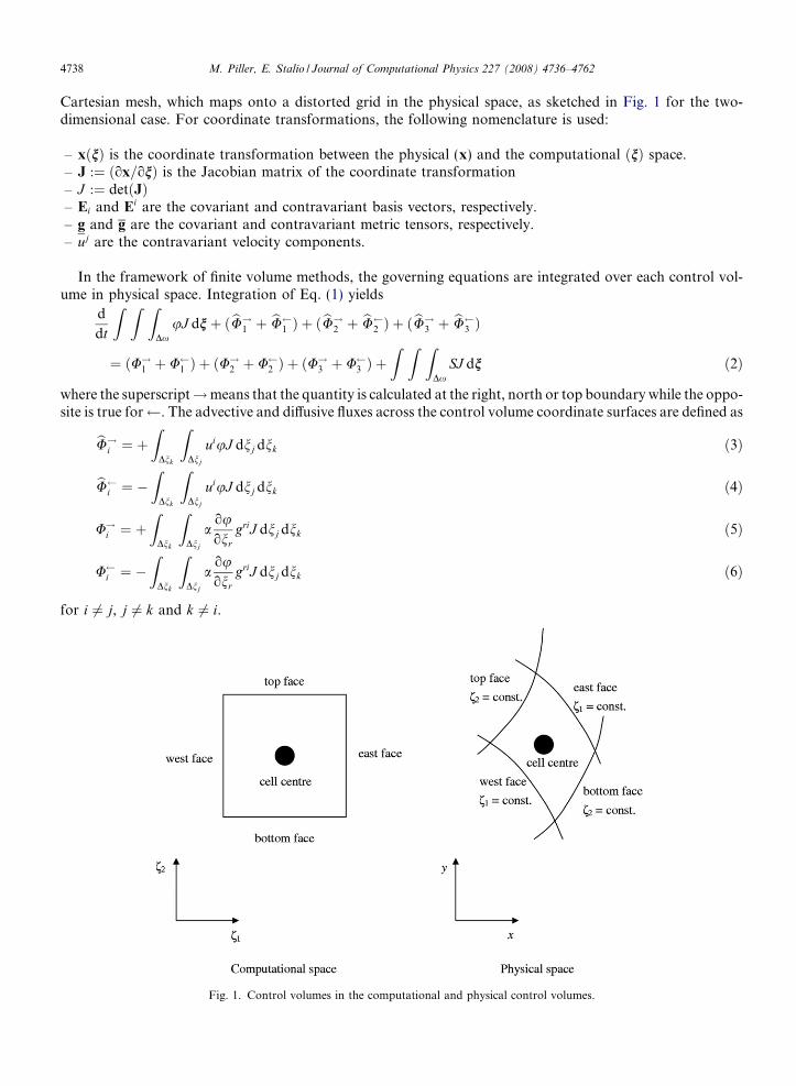
Cartesian mesh, which maps onto a distorted grid in the physical space, as sketched in Fig. 1 for the two-dimensional case. For coordinate transformations, the following nomenclature is used:

– xðnÞ is the coordinate transformation between the physical (x) and the computational ðnÞ space.– J :¼ ðox=onÞ is the Jacobian matrix of the coordinate transformation– J :¼ detðJÞ– Ei and Ei are the covariant and contravariant basis vectors, respectively.– g and g are the covariant and contravariant metric tensors, respectively.– uj are the contravariant velocity components.

In the framework of finite volume methods, the governing equations are integrated over each control vol-ume in physical space. Integration of Eq. (1) yields

d

dt

Z Z ZDx

uJ dnþ ðbU!1 þ bU 1 Þ þ ðbU!2 þ bU 2 Þ þ ðbU!3 þ bU 3 Þ¼ ðU!1 þ U 1 Þ þ ðU!2 þ U 2 Þ þ ðU!3 þ U 3 Þ þ

Z Z ZDx

SJ dn ð2Þ

where the superscript!means that the quantity is calculated at the right, north or top boundary while the oppo-site is true for . The advective and diffusive fluxes across the control volume coordinate surfaces are defined as

bU!i ¼ þ ZDnk

ZDnj

uiuJ dnj dnk ð3Þ

bU i ¼ � ZDnk

ZDnj

uiuJ dnj dnk ð4Þ

U!i ¼ þZ

Dnk

ZDnj

aouonr

griJ dnj dnk ð5Þ

U i ¼ �Z

Dnk

ZDnj

aouonr

griJ dnj dnk ð6Þ

for i 6¼ j, j 6¼ k and k 6¼ i.

Fig. 1. Control volumes in the computational and physical control volumes.


2.2. Numerical formulation

2.2.1. Spatial discretization

2.2.1.1. Field compact schemes. In the present work, the advective fluxes are computed by the conservativefifth-order upwind finite difference scheme proposed by Pirozzoli [26] while the Coupled Derivative finite vol-ume schemes by Kobayashi [12] are used to approximate the diffusive fluxes. Due to the increased number offree parameters C-D schemes attain a higher formal accuracy and better resolution characteristics as com-pared to standard Pade scheme [21,12].

The interpolant and first derivative of a sufficiently smooth function uðxÞ are approximated by C-Dschemes from the cell-averaged values u as follows:
Xm2
k¼�m1

aj;kujþkþ1=2 þ hXp2

k¼�p1

bj;ku0jþkþ1=2 ¼

Xn2

k¼�n1

cj;kujþk ð7Þ

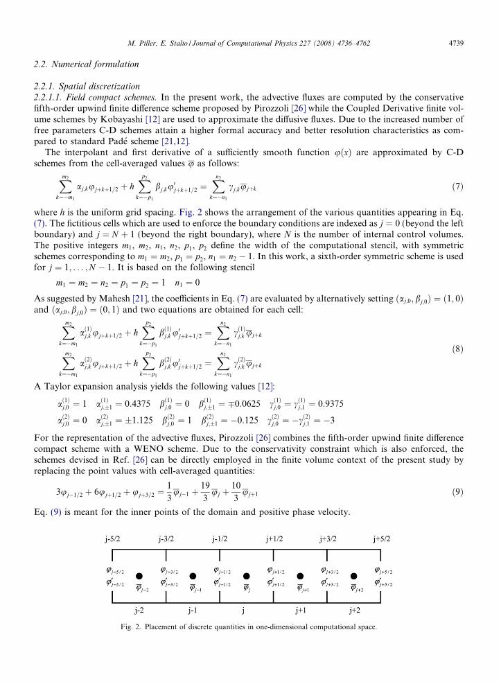
where h is the uniform grid spacing. Fig. 2 shows the arrangement of the various quantities appearing in Eq.(7). The fictitious cells which are used to enforce the boundary conditions are indexed as j ¼ 0 (beyond the leftboundary) and j ¼ N þ 1 (beyond the right boundary), where N is the number of internal control volumes.The positive integers m1, m2, n1, n2, p1, p2 define the width of the computational stencil, with symmetricschemes corresponding to m1 ¼ m2, p1 ¼ p2, n1 ¼ n2 � 1. In this work, a sixth-order symmetric scheme is usedfor j ¼ 1; . . . ;N � 1. It is based on the following stencil

m1 ¼ m2 ¼ n2 ¼ p1 ¼ p2 ¼ 1 n1 ¼ 0

As suggested by Mahesh [21], the coefficients in Eq. (7) are evaluated by alternatively setting ðaj;0; bj;0Þ ¼ ð1; 0Þand ðaj;0; bj;0Þ ¼ ð0; 1Þ and two equations are obtained for each cell:
Xm2
k¼�m1

að1Þj;k ujþkþ1=2 þ hXp2

k¼�p1

bð1Þj;k u0jþkþ1=2 ¼

Xn2

k¼�n1

cð1Þj;k ujþk

Xm2

k¼�m1

að2Þj;k ujþkþ1=2 þ hXp2

k¼�p1

bð2Þj;k u0jþkþ1=2 ¼

Xn2

k¼�n1

cð2Þj;k ujþk

ð8Þ

A Taylor expansion analysis yields the following values [12]:

að1Þj;0 ¼ 1 að1Þj;�1 ¼ 0:4375 bð1Þj;0 ¼ 0 bð1Þj;�1 ¼ �0:0625 cð1Þj;0 ¼ cð1Þj;1 ¼ 0:9375

að2Þj;0 ¼ 0 að2Þj;�1 ¼ �1:125 bð2Þj;0 ¼ 1 bð2Þj;�1 ¼ �0:125 cð2Þj;0 ¼ �cð2Þj;1 ¼ �3

For the representation of the advective fluxes, Pirozzoli [26] combines the fifth-order upwind finite differencecompact scheme with a WENO scheme. Due to the conservativity constraint which is also enforced, theschemes devised in Ref. [26] can be directly employed in the finite volume context of the present study byreplacing the point values with cell-averaged quantities:

3uj�1=2 þ 6ujþ1=2 þ ujþ3=2 ¼1

3uj�1 þ

19

3uj þ

10

3ujþ1 ð9Þ

Eq. (9) is meant for the inner points of the domain and positive phase velocity.

Fig. 2. Placement of discrete quantities in one-dimensional computational space.


2.2.1.2. Schemes for the boundaries. The symmetric schemes of Eqs. (8) and (9) can only be used in the interiornodes of non-periodic domains while special schemes with asymmetric stencil for both differentiation andinterpolation are to be used as the boundary is approached. In this work the boundary conditions are enforcedby introducing a single layer of fictitious cells surrounding the computational domain in transformed space. Asimilar treatment is used, among others, by Pirozzoli [26] in the context of compact finite difference approx-imations. Fictitious cells in physical space do not need to be defined, avoiding any ambiguity in their actualshape. The u values in the fictitious cell of the transformed space become additional unknowns, with the dis-cretized boundary conditions as corresponding equations. This technique allows an easy implementation ofcomplicated boundary conditions especially when residual-based solvers are used, like the Newton–Krylovmethods [24].

Both explicit and compact asymmetric schemes have been used in conjunction with compact schemes forthe inner points. Compact one-sided schemes are considered, among others, by Lele [18], Kobayashi [12], Pil-ler et al. [25], Boersma [2] and Jordan [16]. Explicit schemes are preferred, among others, by Hixon [9] andPirozzoli [26]. In the present work we use explicit one-sided schemes.

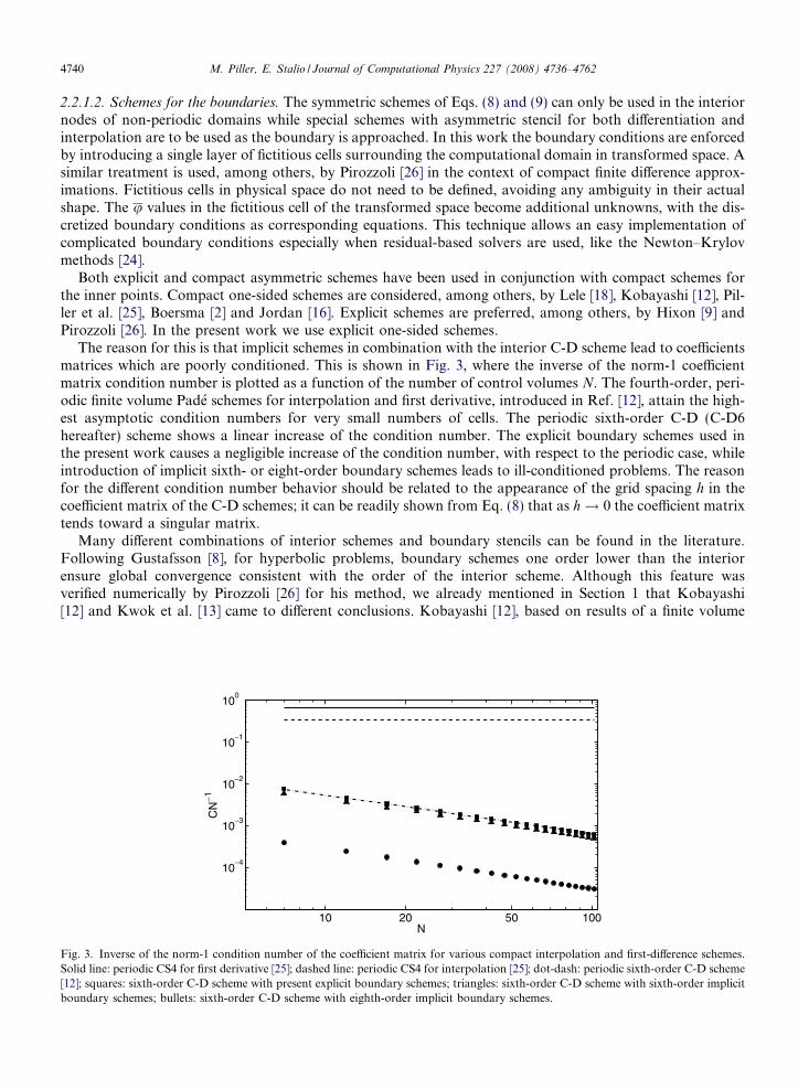
The reason for this is that implicit schemes in combination with the interior C-D scheme lead to coefficientsmatrices which are poorly conditioned. This is shown in Fig. 3, where the inverse of the norm-1 coefficientmatrix condition number is plotted as a function of the number of control volumes N. The fourth-order, peri-odic finite volume Pade schemes for interpolation and first derivative, introduced in Ref. [12], attain the high-est asymptotic condition numbers for very small numbers of cells. The periodic sixth-order C-D (C-D6hereafter) scheme shows a linear increase of the condition number. The explicit boundary schemes used inthe present work causes a negligible increase of the condition number, with respect to the periodic case, whileintroduction of implicit sixth- or eight-order boundary schemes leads to ill-conditioned problems. The reasonfor the different condition number behavior should be related to the appearance of the grid spacing h in thecoefficient matrix of the C-D schemes; it can be readily shown from Eq. (8) that as h! 0 the coefficient matrixtends toward a singular matrix.

Many different combinations of interior schemes and boundary stencils can be found in the literature.Following Gustafsson [8], for hyperbolic problems, boundary schemes one order lower than the interiorensure global convergence consistent with the order of the interior scheme. Although this feature wasverified numerically by Pirozzoli [26] for his method, we already mentioned in Section 1 that Kobayashi[12] and Kwok et al. [13] came to different conclusions. Kobayashi [12], based on results of a finite volume

10 20 50 100

10−4

10−3

10−2

10−1

100

N

CN

−1

Fig. 3. Inverse of the norm-1 condition number of the coefficient matrix for various compact interpolation and first-difference schemes.Solid line: periodic CS4 for first derivative [25]; dashed line: periodic CS4 for interpolation [25]; dot-dash: periodic sixth-order C-D scheme[12]; squares: sixth-order C-D scheme with present explicit boundary schemes; triangles: sixth-order C-D scheme with sixth-order implicitboundary schemes; bullets: sixth-order C-D scheme with eighth-order implicit boundary schemes.


simulation of the one-dimensional, steady advection–diffusion equation, shows that the quality of solutionsobtained with C-D schemes is even more affected by the boundary closure than for traditional Padeschemes, and that for C-D schemes the overall order of accuracy is given by the near-boundary compactschemes. On the other hand, Mahesh [21] develops templates formed by a sixth-order symmetric C-D finitedifference scheme in the interior and third-, fourth- or fifth-order C-D boundary schemes and verifiesnumerically that only the third-order scheme results in asymptotically stable solutions of the one-dimen-sional linear advection equation.

In the present work, the explicit schemes used next to the boundaries are at least of the same order of accu-racy as the interior schemes.

For the discretization of the advective term next to the boundaries, fourth-order, explicit, one-sided bound-ary schemes are used in the present work, as introduced in Ref. [26]. For positive phase speed they result

u1=2 ¼1

4u0 þ

13

12u1 �

5

12u2 þ

1

12u3 ð10Þ

uNþ1=2 ¼25

12uN �

23

12uN�1 þ

13

12uN�2 �

1

4uN�3 ð11Þ

The approximation (10) is used at inflow boundaries, while (11) applies at outflow boundaries. Since (11) doesnot include the fictitious cell, which however is considered as unknown in the present work, care is taken inorder to avoid that the system of equations becomes singular.

2.2.1.3. Deconvolution. As stated in Ref. [22], deconvolution is the restoration of signals degraded by a con-volution operator. In the context of high-order finite volume discretization, deconvolution is required in orderto recover a pointwise representation of a quantity from the knowledge of its mean values over a set of controlvolumes. This distinction is unnecessary for second-order finite volume discretization but becomes substantialwhen high-order schemes are employed. While Pereira et al. [24] and Piller et al. [25] use compact deconvo-lution schemes, in the present work explicit schemes are preferred because they can be more easily adaptedto the desired order of accuracy.

With reference to the one-dimensional case, the aim is to recover f ðnÞ from knowledge of f ðnÞ, where

�f ðnÞ ¼ 1

Dn

Z nþDn=2

n�Dn=2

f ðfÞdf ð12Þ

Let us assume that the values f i, �f iþ1, . . ., �f iþm are known and we aim to approximate f ðnÞ at some point n. Tothis end, we expand f as

f ðnÞ � bf ðnÞ ¼Xm

j¼0

ajP jðnÞ

where fP jðnÞgmj¼0 is a set of linearly-independent polynomials with P j of order j and bf is an approximation to f.

The mþ 1 conditions

�f iþk ¼ �f iþk; k ¼ 0; 1; . . . ;m ð13Þ
allow to compute the coefficients aj. Eq. (13) can be written in matrix form:
�f ¼ Pa ð14Þ
where
P :¼ ½P ji �; P j

i :¼ 1

Dn

Z nþDn=2

n�Dn=2

P iðnÞdn

and the approximated value bf ðnÞ can be computed by
bf ðnÞ ¼Xj
P jðnÞaj ¼ ½P 0ðnÞ . . . P mðnÞ�a :¼ Pa ð15Þ


with

P :¼ ½P 0ðnÞ . . . P mðnÞ�
Substitution of Eq. (14) into (15) yields
f ðnÞ ¼ PP�1�f :¼ ½bg0ðnÞ . . . bgmðnÞ��f
it is apparent that the Lagrange-like functions gjðnÞ may be precomputed at n ¼ n by solving the system (14)with mþ 1 different right-hand sides, corresponding to the canonical unit vectors of Rmþ1.
With regard to the existence and uniqueness of such an approximation, the problem is equivalent to findingthe conditions for the coefficient matrix in Eq. (14) to be non-singular. Such conditions can be found from thetheory of pointwise interpolation. The primitive function of f is introduced

F ðnÞ :¼Z n

0

f ðgÞdg

so that

�f ðnÞ :¼ 1

Dn

Z nþDn=2

n�Dn=2

f ðgÞdg ¼ 1

Dn½F ðnþ Dn=2Þ � F ðn� Dn=2Þ�

Since similar definitions and identities apply to the approximation function f ðnÞ, conditions (13) may be recastas

1

Dn½F ðnk þ Dn=2Þ � F ðnk � Dn=2Þ� ¼ 1

Dn½bF ðnk þ Dn=2Þ � bF ðnk � Dn=2Þ� 8k ¼ 0; . . . ;m ð16Þ

this implies that the two sequences

fF ðn0 � Dn=2Þ; F ðn1 � Dn=2Þ; . . . ; F ðnm þ Dn=2ÞgfbF ðn0 � Dn=2Þ; bF ðn1 � Dn=2Þ; . . . ; bF ðnm þ Dn=2Þg

differ at most by an additive constant. Therefore, the problem of finding bf is equivalent to finding the point-wise interpolant bF to F through the mþ 1 points nk � Dn=2, k ¼ 1; . . . ;mþ 1 while setting bF ðn0 � Dn=2Þ to anarbitrary value. In the case of polynomial interpolation, such an interpolant exists and is unique as long as themþ 1 interpolation nodes are distinct and the degree of the interpolation polynomial is not higher than m.

Multi-dimensional deconvolution can be obtained by tensor-product of the one-dimensional interpolantbasis [3]. This corresponds to interpolating independently and in sequence along each coordinate direction,

bf ðn1; n2; n3Þ ¼Xm3

i3¼0

Xm2

i2¼0

Xm1

i1¼0

�f iþi1;jþi2;kþi3bgiþi1ðn1Þbgjþi2ðn2Þbgkþi3ðn3Þ ð17Þ

The reconstruction of a function f onto a set of quadrature nodes can be made considerably more efficient byusing the sum-factorization technique [10]. With reference to Eq. (17), the sum-factorization results in

f q1;q2;q3¼Xm3

i3¼0

Xm2

i2¼0

Xm1

i1¼0

�f i1;i2;i3 gi1;q1gi2;q2

gi3;q3¼Xm3

i3¼0

bgi3;q3

Xm2

i2¼0

bgi2;q2

Xm1

i1¼0gi1;q1

�f i1;i2;i3|fflfflfflfflfflfflfflfflfflfflfflfflffl{zfflfflfflfflfflfflfflfflfflfflfflfflffl}Aq1 ;i2 ;i3

¼X

i3

gi3;q3

Xi2

gi2;q2Aq1;i2;i3|fflfflfflfflfflfflfflfflfflfflfflffl{zfflfflfflfflfflfflfflfflfflfflfflffl}

Bq1 ;q2 ;i3

¼X

i3

gi3;q3Bq1;q2;i3 ð18Þ

where the indices i1, i2, i3 refer to the basis functions, while q1, q2, q3 identify the quadrature nodes, respec-tively. The sum-factorization technique reduces the complexity of the deconvolution from order 6 to order 4.

2.2.1.4. Flux representation. In this section, a high-order procedure is presented, for the discretization of dif-fusive and advective fluxes on non-orthogonal curvilinear grids.


Focusing on the orthogonal diffusive flux across the east coordinate surface DSe of a control volume, thefollowing term must be discretized:
Z Z
DSe

aouon1

g1;1J dn2 dn3 ð19Þ

three integrals need to be computed for this purpose

1

Dn2Dn3

ZDn3

ZDn2

adn2 dn3 ð20Þ

1

Dn2Dn3

ZDn3

ZDn2

ouon1

dn2 dn3 ð21Þ

1

Dn2Dn3

ZDn3

ZDn2


Assuming that the diffusion coefficient a depends on x, t and u, it can be evaluated at the Gauss–Legendrequadrature nodes once u has been computed at the same locations. This is achieved by applying the decon-volution procedure described in Section 2.2.1.3 to the face-averaged values of u, which in turn are computedfrom the cell-averaged values by compact interpolation along n1. Then, Gauss–Legendre quadrature on thecell face yields the required approximation of (20). The second term (21) is evaluated directly by the compactinterpolation scheme presented in Section 2.2.1.1. The third contribution, Eq. (22), is computed and storedafter the calculation of the metric terms. Once the contributions (20) and (21) are available, the deconvolutionprocedure outlined in Section 2.2.1.3 is used once more to evaluate the integrand functions in Eqs. (20)–(22) atthe quadrature nodes of the cell face considered. Gauss quadrature of the product of the three integrandsyields the desired approximation for (19).

The discretization procedure for the cross-diffusive fluxes is presented for the term
Z ZDSe
aouon2


In order to evaluate the integral in Eq. (23), the following face-averaged contributions are needed in compu-tational space:

1

Dn2Dn3

ZDn3

ZDn2

adn2 dn3 ð24Þ

1

Dn2Dn3

ZDn3

ZDn2

ouon2

dn2 dn3 ð25Þ

1

Dn2Dn3

ZDn3

ZDn2


After these expressions have been calculated, they can be used to obtain an approximation of (23) by followingthe same procedure outlined for the evaluation of the orthogonal diffusive fluxes. Integrals (24) and (26) arecomputed as (20) and (22), respectively. The diffusive term (25) can be evaluated by first integrating along n2

with no approximation:

1

DSe

Z ZDS1

ouon2

dn2 dn3 ¼1

Dn3

ZDn3

uiþ1=2;jþ1=2;k � uiþ1=2;j�1=2;k

Dn2

dn3 ¼un3

iþ1=2;jþ1=2;k � un3

iþ1=2;j�1=2;k

Dn2

ð27Þ

then, the terms un3

iþ1=2;j�1=2;k can be evaluated by either of two compact interpolations, along n2 or along n1.The approximation of the advective fluxes is based on the same general technique used for the diffusive

fluxes. Considering the flux bU!1 defined in Eq. (3), the cell face averages of u1J and u are computed by thecompact schemes (9)–(11). Then, the deconvolution procedure described in Section 2.2.1.3 followed byGauss–Legendre quadrature is used to obtain the advective flux (3).

The flux representation procedure described above is used also to enforce the boundary conditions withhigh-order accuracy. The third-kind (Robin) boundary conditions in boundary-fitted coordinates, for aðn2; n3Þ boundary surface, yield


0 ¼Z

Dn3

ZDn2

a1

ouonk

gk1J þ ða2uþ a3Þffiffiffiffiffiffiffig1;1

pJ

� �dn2 dn3 ð28Þ

where in general coefficients a1, a2, a3 depend on both position and time. The discrete representation of (28) isobtained following the procedure presented in Section 2.2.1.4. The resulting algebraic equation is added to theset of discretized conservation equations for the internal control volumes.

2.2.2. Fourier analysisIn this section the resolution properties of the spatial discretization schemes employed in the proposed

numerical algorithm are investigated by Fourier analysis. Classical Fourier analysis [30,12] is used to accessthe properties of interior schemes under the assumption of periodic boundary conditions. The focus is onthe C-D6 schemes used for the spatial discretization of the diffusion equation because the resolution propertiesof the upwind scheme used for the discretization of the advective term has been thoroughly investigated byPirozzoli [26].

2.2.2.1. Resolution properties. The analysis is based on the one-dimensional diffusion equation with complexexponential initial conditions:

ouot ¼ a o2u

ox2

uðx; 0Þ ¼ eikx

(ð29Þ

and periodic boundary conditions. The cell-averaged analytical solution to Eq. (29) reads

ujðtÞ ¼ ujð0ÞF ðKÞ expð�FoK2Þ ð30Þ
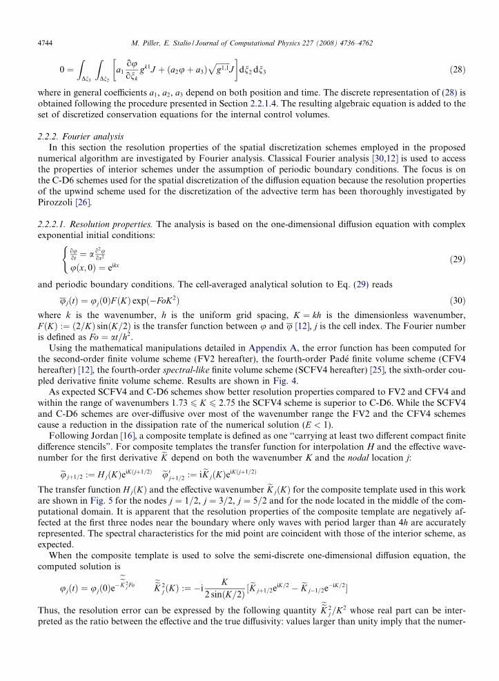
where k is the wavenumber, h is the uniform grid spacing, K ¼ kh is the dimensionless wavenumber,F ðKÞ :¼ ð2=KÞ sinðK=2Þ is the transfer function between u and u [12], j is the cell index. The Fourier numberis defined as Fo ¼ at=h2.
Using the mathematical manipulations detailed in Appendix A, the error function has been computed forthe second-order finite volume scheme (FV2 hereafter), the fourth-order Pade finite volume scheme (CFV4hereafter) [12], the fourth-order spectral-like finite volume scheme (SCFV4 hereafter) [25], the sixth-order cou-pled derivative finite volume scheme. Results are shown in Fig. 4.

As expected SCFV4 and C-D6 schemes show better resolution properties compared to FV2 and CFV4 andwithin the range of wavenumbers 1:73 6 K 6 2:75 the SCFV4 scheme is superior to C-D6. While the SCFV4and C-D6 schemes are over-diffusive over most of the wavenumber range the FV2 and the CFV4 schemescause a reduction in the dissipation rate of the numerical solution (E < 1).

Following Jordan [16], a composite template is defined as one ‘‘carrying at least two different compact finitedifference stencils”. For composite templates the transfer function for interpolation H and the effective wave-number for the first derivative eK depend on both the wavenumber K and the nodal location j:
eujþ1=2 :¼ HjðKÞeiKðjþ1=2Þ eu 0jþ1=2 :¼ ieK jðKÞeiKðjþ1=2Þ
The transfer function HjðKÞ and the effective wavenumber eK jðKÞ for the composite template used in this workare shown in Fig. 5 for the nodes j ¼ 1=2, j ¼ 3=2, j ¼ 5=2 and for the node located in the middle of the com-putational domain. It is apparent that the resolution properties of the composite template are negatively af-fected at the first three nodes near the boundary where only waves with period larger than 4h are accuratelyrepresented. The spectral characteristics for the mid point are coincident with those of the interior scheme, asexpected.

When the composite template is used to solve the semi-discrete one-dimensional diffusion equation, thecomputed solution is

ujðtÞ ¼ ujð0Þe�eeK 2

j Fo eeK 2j ðKÞ :¼ �i

K2 sinðK=2Þ ½

eK jþ1=2eiK=2 � eK j�1=2e�iK=2�

Thus, the resolution error can be expressed by the following quantityeeK 2

j=K2 whose real part can be inter-preted as the ratio between the effective and the true diffusivity: values larger than unity imply that the numer-

0 0.5 1 1.5 2 2.5 3

0.5

0.6

0.7

0.8

0.9

1

K

E1D

Fig. 4. Error function for the one-dimensional diffusion equation, obtained by Fourier analysis. —: FV2; - - -: CFV4; –�–: SCFV4; � � �:C-D6.

0 20

0.5

1

1.5

2

2.5

kh

Re(

H)

0 2

0

0.5

1

1.5

2

2.5

3

kh

Im(H

)

0 2−4

−3

−2

−1

0

1

2

3

kh

Re(

k effh)

0 2

0

0.5

1

1.5

2

2.5

3

3.5

4

4.5

kh

Im(k

effh)

Fig. 5. (a) (Left) Real and (right) imaginary parts of the transfer function for interpolation for the composite template. (b) (Left) Real and(right) imaginary parts of the effective wavenumber for the composite template. � � �: node j ¼ 1=2; - - -: node j ¼ 3=2; –�–: node j ¼ 5=2; : mid point.



ical solution decays faster than the exact solution. The imaginary part ofeeK 2

j=K2 can be recast in terms of a cellPeclet number as

Fig. 6.for thecompacell j ¼

Fig. 7

PejðKÞ :¼ echa¼

imagð eeK 2j Þ

K

where ec is a numerical phase velocity. Pej is identically zero for the exact solution and represents a dispersionerror in the computed solution.

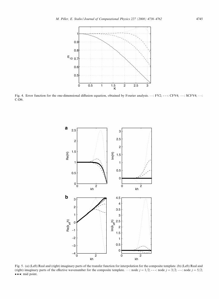
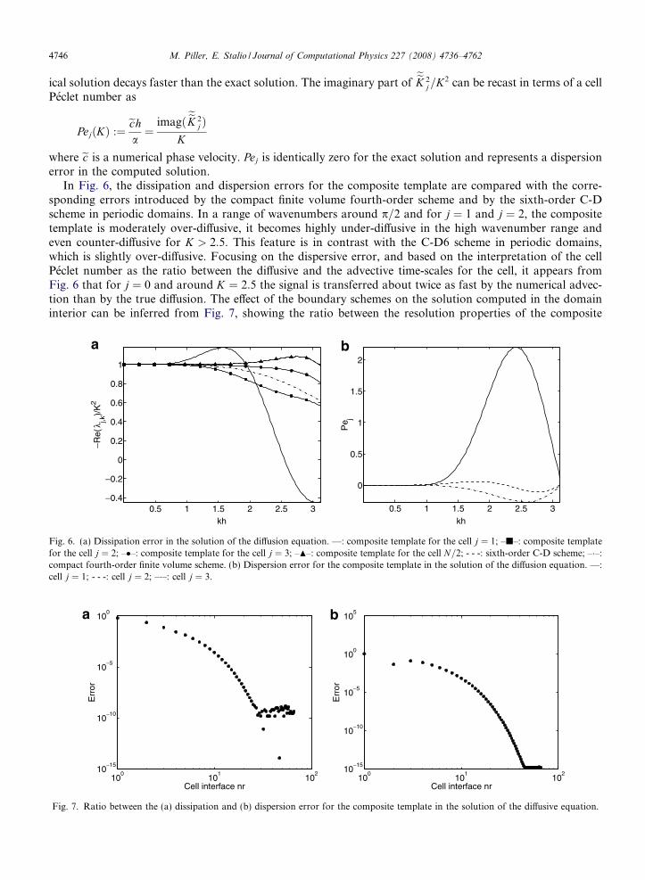
In Fig. 6, the dissipation and dispersion errors for the composite template are compared with the corre-sponding errors introduced by the compact finite volume fourth-order scheme and by the sixth-order C-Dscheme in periodic domains. In a range of wavenumbers around p=2 and for j ¼ 1 and j ¼ 2, the compositetemplate is moderately over-diffusive, it becomes highly under-diffusive in the high wavenumber range andeven counter-diffusive for K > 2:5. This feature is in contrast with the C-D6 scheme in periodic domains,which is slightly over-diffusive. Focusing on the dispersive error, and based on the interpretation of the cellPeclet number as the ratio between the diffusive and the advective time-scales for the cell, it appears fromFig. 6 that for j ¼ 0 and around K ¼ 2:5 the signal is transferred about twice as fast by the numerical advec-tion than by the true diffusion. The effect of the boundary schemes on the solution computed in the domaininterior can be inferred from Fig. 7, showing the ratio between the resolution properties of the composite

0.5 1 1.5 2 2.5 3−0.4

−0.2

0

0.2

0.4

0.6

0.8

1

kh

−Re(

λ j,k)/

K2

0.5 1 1.5 2 2.5 3

0

0.5

1

1.5

2

kh

Pe j

(a) Dissipation error in the solution of the diffusion equation. —: composite template for the cell j ¼ 1; –j–: composite templatecell j ¼ 2; ––: composite template for the cell j ¼ 3; –N–: composite template for the cell N=2; - - -: sixth-order C-D scheme; –�–:

ct fourth-order finite volume scheme. (b) Dispersion error for the composite template in the solution of the diffusion equation. —:1; - - -: cell j ¼ 2; –�–: cell j ¼ 3.

100

101

102

10−15

10−10

10−5

100

Cell interface nr

Err

or

100

101

102

10−15

10−10

10−5

100

105

Cell interface nr

Err

or

. Ratio between the (a) dissipation and (b) dispersion error for the composite template in the solution of the diffusive equation.


template represented in Fig. 6 with the corresponding quantities for the sixth-order C-D scheme in a periodicdomain. It is evident that both the dissipation and the dispersion errors induced by the boundary schemesdecay very fast when moving toward the domain interior.

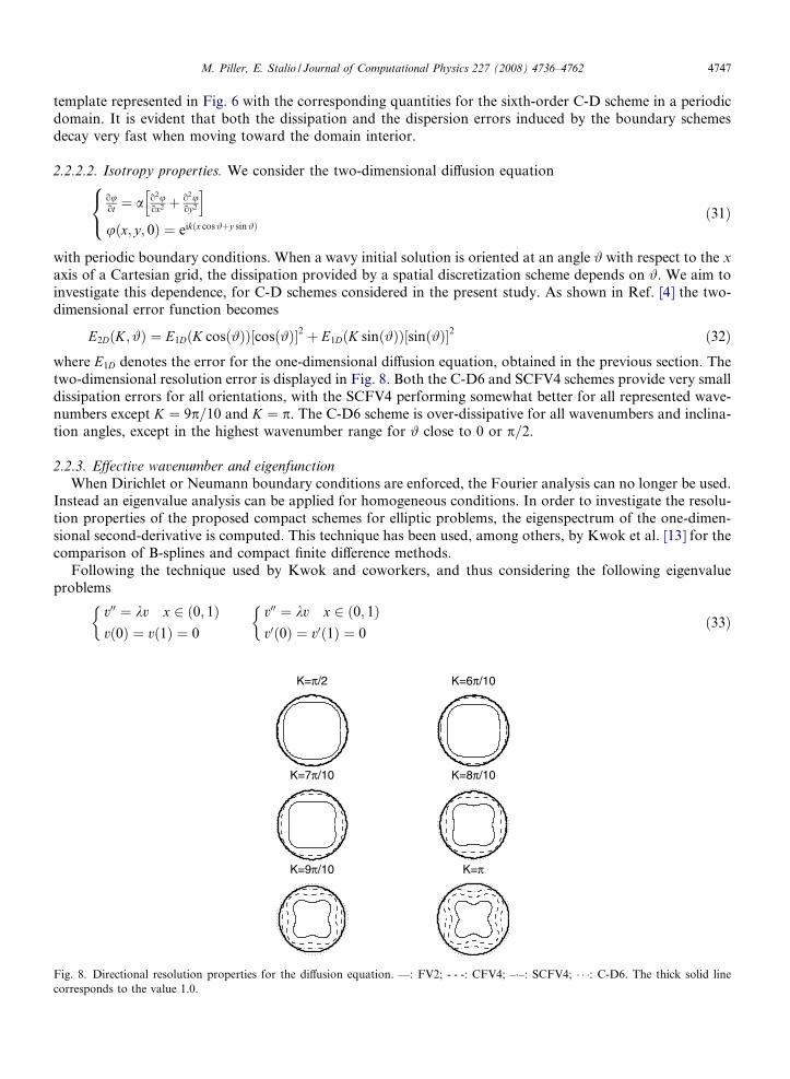
2.2.2.2. Isotropy properties. We consider the two-dimensional diffusion equation

Fig. 8.corresp

ouot ¼ a o2u

ox2 þ o2uoy2

h iuðx; y; 0Þ ¼ eikðx cos #þy sin#Þ

8<: ð31Þ

with periodic boundary conditions. When a wavy initial solution is oriented at an angle # with respect to the x

axis of a Cartesian grid, the dissipation provided by a spatial discretization scheme depends on #. We aim toinvestigate this dependence, for C-D schemes considered in the present study. As shown in Ref. [4] the two-dimensional error function becomes

E2DðK; #Þ ¼ E1DðK cosð#ÞÞ½cosð#Þ�2 þ E1DðK sinð#ÞÞ½sinð#Þ�2 ð32Þ
where E1D denotes the error for the one-dimensional diffusion equation, obtained in the previous section. Thetwo-dimensional resolution error is displayed in Fig. 8. Both the C-D6 and SCFV4 schemes provide very smalldissipation errors for all orientations, with the SCFV4 performing somewhat better for all represented wave-numbers except K ¼ 9p=10 and K ¼ p. The C-D6 scheme is over-dissipative for all wavenumbers and inclina-tion angles, except in the highest wavenumber range for # close to 0 or p=2.
2.2.3. Effective wavenumber and eigenfunction

When Dirichlet or Neumann boundary conditions are enforced, the Fourier analysis can no longer be used.Instead an eigenvalue analysis can be applied for homogeneous conditions. In order to investigate the resolu-tion properties of the proposed compact schemes for elliptic problems, the eigenspectrum of the one-dimen-sional second-derivative is computed. This technique has been used, among others, by Kwok et al. [13] for thecomparison of B-splines and compact finite difference methods.

Following the technique used by Kwok and coworkers, and thus considering the following eigenvalueproblems

v00 ¼ kv x 2 ð0; 1Þvð0Þ ¼ vð1Þ ¼ 0

�v00 ¼ kv x 2 ð0; 1Þv0ð0Þ ¼ v0ð1Þ ¼ 0

�ð33Þ

K=π/2 K=6π/10

K=7π/10 K=8π/10

K=9π/10 K=π

Directional resolution properties for the diffusion equation. —: FV2; - - -: CFV4; –�–: SCFV4; � � �: C-D6. The thick solid lineonds to the value 1.0.


The eigenvalues for both problems (33) are

Fig. 9.boundboundorder.

TableResolv

Schem

FV2C-D6C-D12

kk ¼ �ðpkÞ2 ð34Þ
once represented in the finite volume context
1

h½v0jþ1=2 � v0j�1=2� ¼ k�vj ð35Þ

can be recast as

D�v ¼ k�v ð36Þ
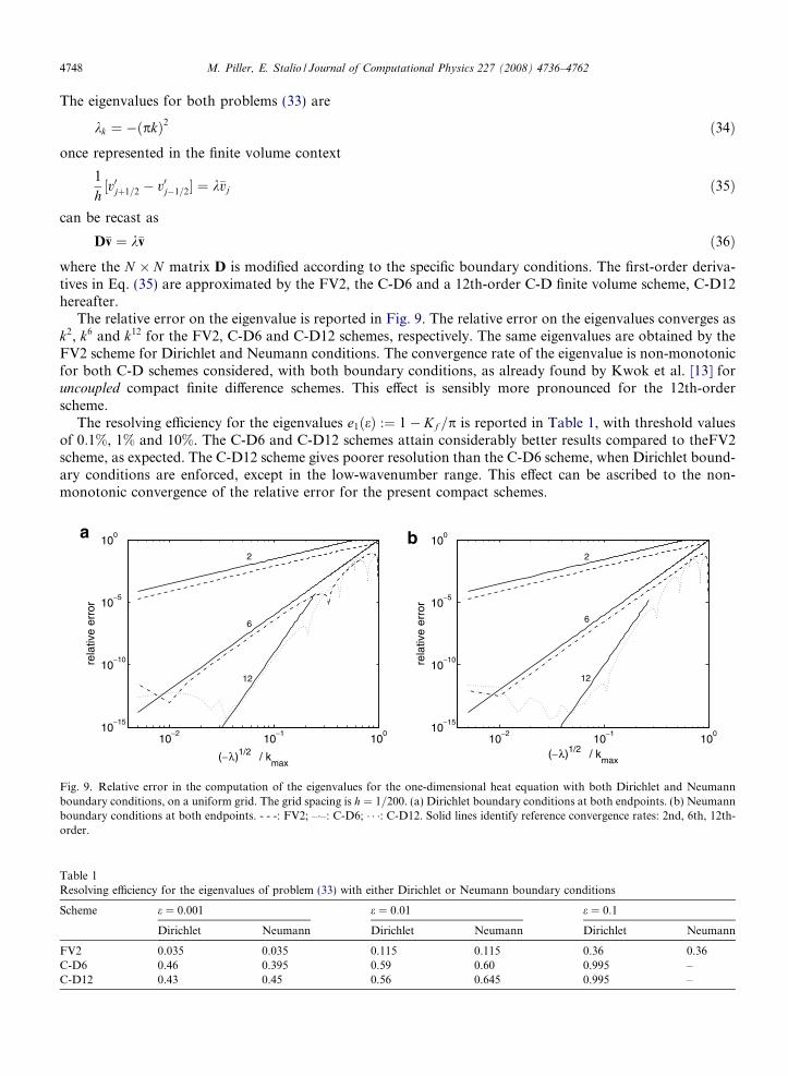
where the N � N matrix D is modified according to the specific boundary conditions. The first-order deriva-tives in Eq. (35) are approximated by the FV2, the C-D6 and a 12th-order C-D finite volume scheme, C-D12hereafter.
The relative error on the eigenvalue is reported in Fig. 9. The relative error on the eigenvalues converges ask2, k6 and k12 for the FV2, C-D6 and C-D12 schemes, respectively. The same eigenvalues are obtained by theFV2 scheme for Dirichlet and Neumann conditions. The convergence rate of the eigenvalue is non-monotonicfor both C-D schemes considered, with both boundary conditions, as already found by Kwok et al. [13] foruncoupled compact finite difference schemes. This effect is sensibly more pronounced for the 12th-orderscheme.

The resolving efficiency for the eigenvalues e1ðeÞ :¼ 1� Kf =p is reported in Table 1, with threshold valuesof 0:1%, 1% and 10%. The C-D6 and C-D12 schemes attain considerably better results compared to theFV2scheme, as expected. The C-D12 scheme gives poorer resolution than the C-D6 scheme, when Dirichlet bound-ary conditions are enforced, except in the low-wavenumber range. This effect can be ascribed to the non-monotonic convergence of the relative error for the present compact schemes.

10−2

10−1

100

10−15

10−10

10−5

100

2

6

12

(−λ)1/2 / kmax

rela

tive

erro

r

10−2

10−1

100

10−15

10−10

10−5

100

2

6

12

(−λ)1/2 / kmax

rela

tive

erro

r

Relative error in the computation of the eigenvalues for the one-dimensional heat equation with both Dirichlet and Neumannary conditions, on a uniform grid. The grid spacing is h ¼ 1=200. (a) Dirichlet boundary conditions at both endpoints. (b) Neumannary conditions at both endpoints. - - -: FV2; –�–: C-D6; � � �: C-D12. Solid lines identify reference convergence rates: 2nd, 6th, 12th-

1ing efficiency for the eigenvalues of problem (33) with either Dirichlet or Neumann boundary conditions

e e ¼ 0:001 e ¼ 0:01 e ¼ 0:1

Dirichlet Neumann Dirichlet Neumann Dirichlet Neumann

0.035 0.035 0.115 0.115 0.36 0.360.46 0.395 0.59 0.60 0.995 –0.43 0.45 0.56 0.645 0.995 –


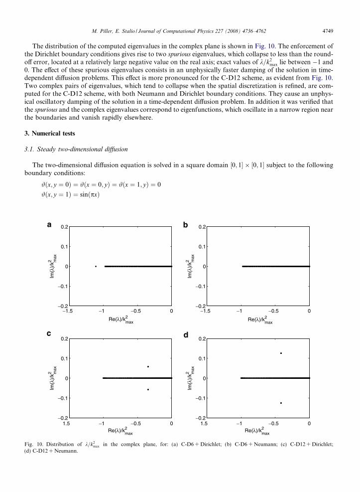
The distribution of the computed eigenvalues in the complex plane is shown in Fig. 10. The enforcement ofthe Dirichlet boundary conditions gives rise to two spurious eigenvalues, which collapse to less than the round-off error, located at a relatively large negative value on the real axis; exact values of k=k2

max lie between �1 and0. The effect of these spurious eigenvalues consists in an unphysically faster damping of the solution in time-dependent diffusion problems. This effect is more pronounced for the C-D12 scheme, as evident from Fig. 10.Two complex pairs of eigenvalues, which tend to collapse when the spatial discretization is refined, are com-puted for the C-D12 scheme, with both Neumann and Dirichlet boundary conditions. They cause an unphys-ical oscillatory damping of the solution in a time-dependent diffusion problem. In addition it was verified thatthe spurious and the complex eigenvalues correspond to eigenfunctions, which oscillate in a narrow region nearthe boundaries and vanish rapidly elsewhere.

3. Numerical tests

3.1. Steady two-dimensional diffusion

The two-dimensional diffusion equation is solved in a square domain ½0; 1� � ½0; 1� subject to the followingboundary conditions:

Fig. 1(d) C-D

#ðx; y ¼ 0Þ ¼ #ðx ¼ 0; yÞ ¼ #ðx ¼ 1; yÞ ¼ 0

#ðx; y ¼ 1Þ ¼ sinðpxÞ

−1.5 −1 −0.5 0−0.2

−0.1

0

0.1

0.2

Re(λ)/kmax2

Im(λ

)/k m

ax2

−1.5 −1 −0.5 0−0.2

−0.1

0

0.1

0.2

Re(λ)/kmax2

Im(λ

)/k m

ax2

1.5 −1 −0.5 0−0.2

−0.1

0

0.1

0.2

Re(λ)/kmax2

Im(λ

)/k m

ax2

1.5 −1 −0.5 0−0.2

−0.1

0

0.1

0.2

Re(λ)/kmax2

Im(λ

)/k m

ax2

0. Distribution of k=k2max in the complex plane, for: (a) C-D6 + Dirichlet; (b) C-D6 + Neumann; (c) C-D12 + Dirichlet;

12 + Neumann.


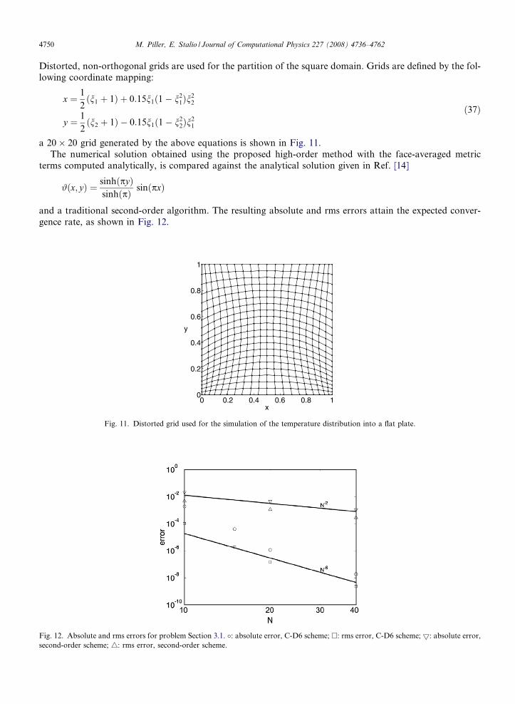
Distorted, non-orthogonal grids are used for the partition of the square domain. Grids are defined by the fol-lowing coordinate mapping:

Fig. 12second

x ¼ 1

2ðn1 þ 1Þ þ 0:15n1ð1� n2

1Þn22

y ¼ 1

2ðn2 þ 1Þ � 0:15n1ð1� n2

2Þn21

ð37Þ

a 20� 20 grid generated by the above equations is shown in Fig. 11.The numerical solution obtained using the proposed high-order method with the face-averaged metric

terms computed analytically, is compared against the analytical solution given in Ref. [14]

#ðx; yÞ ¼ sinhðpyÞsinhðpÞ sinðpxÞ

and a traditional second-order algorithm. The resulting absolute and rms errors attain the expected conver-gence rate, as shown in Fig. 12.

0 0.2 0.4 0.6 0.8 10

0.2

0.4

0.6

0.8

1

x

y

Fig. 11. Distorted grid used for the simulation of the temperature distribution into a flat plate.

. Absolute and rms errors for problem Section 3.1. �: absolute error, C-D6 scheme; �: rms error, C-D6 scheme; 5: absolute error,-order scheme; 4: rms error, second-order scheme.


3.2. Unsteady diffusion

In this section, the simulation of unsteady thermal diffusion is presented in order to provide evidence thatthe present finite volume formulation can be applied to the solution of time-dependent diffusion phenomena.The physical domain is represented by a plane slab with homogeneous thermal diffusivity. Initially the slab hasa uniform temperature distribution T i. The temperature field evolves in time driven by the heat exchangethrough the right boundary which is exposed to a fluid of unperturbed temperature T1. The left, upperand lower boundaries are adiabatic. The relevant quantities are scaled by the slab thickness L, the diffusivetime-scale L2=a and the temperature difference T i � T1, yielding to

oHoFo¼ o2H

ox2þ o2H

oy2ðx; yÞ 2 ½0; 1�

Hðx; y; Fo ¼ 0Þ ¼ 1

oHox¼ 0 at x ¼ 0; Fo > 0

oHoxþ BiH ¼ 0 at x ¼ 1; Fo > 0

oHoy¼ 0 at y ¼ 0; Fo > 0

oHoy¼ 0 at y ¼ 2; Fo > 0

ð38Þ

where x :¼ x=L, y :¼ y=L, H :¼ ðT � T1Þ=ðT i � T1Þ, Fo :¼ at=L2 is the Fourier number, Bi :¼ hL=k is theBiot number. The initial value problem (38) has analytical, one-dimensional solution given in Ref. [14].Numerical and analytical solutions for a constant Biot number Bi ¼ 4:0 are compared over a dimensionlesstime interval 0 6 Fo 6 0:5.

The rectangular domain is discretized with the distorted grids defined by Eq. (37) and the metrics of thetransformation are evaluated analytically. Time integration is performed by an implicit second-order predic-tor–corrector scheme [1]. During the time integration, the time-step is progressively reduced in order to keepthe cell Fourier number Foc :¼ aDt=h2 approximately constant.

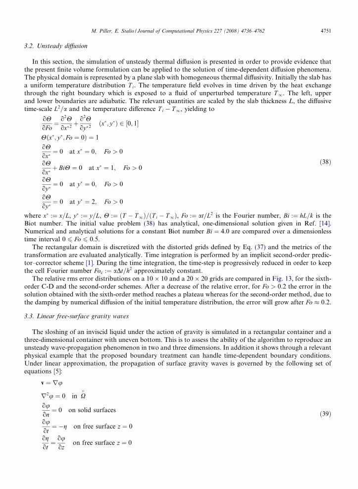
The relative rms error distributions on a 10� 10 and a 20� 20 grids are compared in Fig. 13, for the sixth-order C-D and the second-order schemes. After a decrease of the relative error, for Fo > 0:2 the error in thesolution obtained with the sixth-order method reaches a plateau whereas for the second-order method, due tothe damping by numerical diffusion of the initial temperature distribution, the error will grow after Fo � 0:2.

3.3. Linear free-surface gravity waves

The sloshing of an inviscid liquid under the action of gravity is simulated in a rectangular container and athree-dimensional container with uneven bottom. This is to assess the ability of the algorithm to reproduce anunsteady wave-propagation phenomenon in two and three dimensions. In addition it shows through a relevantphysical example that the proposed boundary treatment can handle time-dependent boundary conditions.Under linear approximation, the propagation of surface gravity waves is governed by the following set ofequations [5]:

v ¼ ru

r2u ¼ 0 in X�

ouon¼ 0 on solid surfaces

ouot¼ �g on free surface z ¼ 0

ogot¼ ou

ozon free surface z ¼ 0

ð39Þ

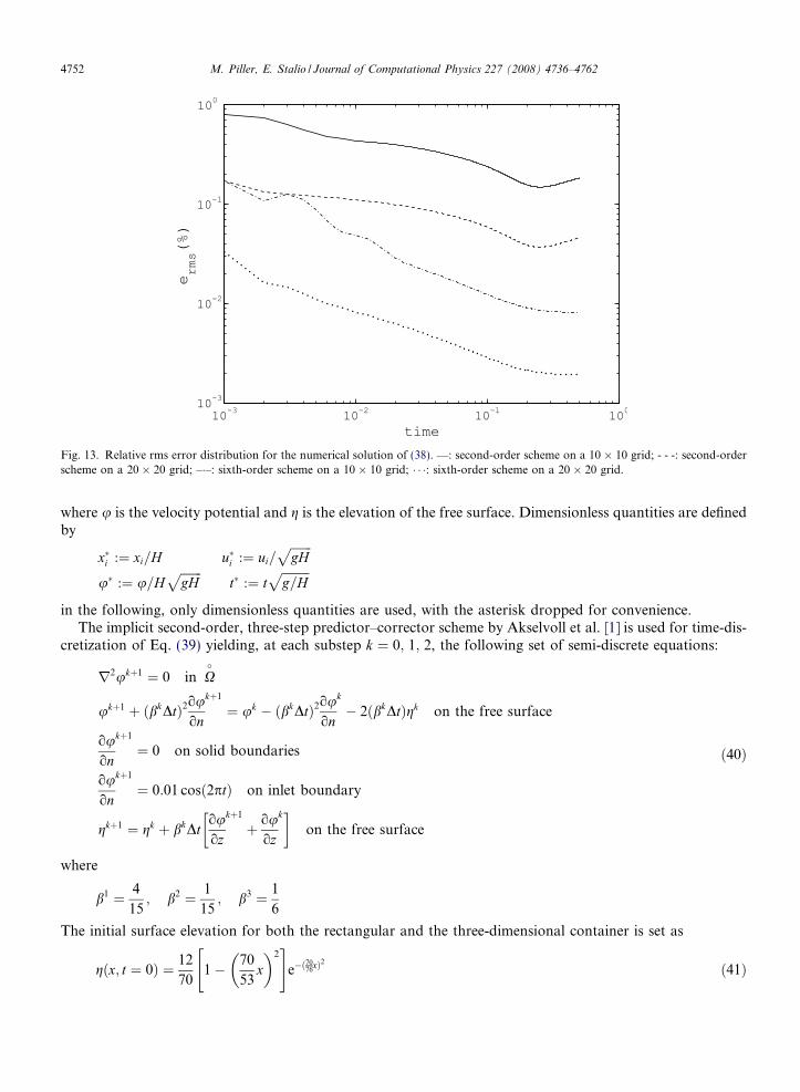
Fig. 13. Relative rms error distribution for the numerical solution of (38). —: second-order scheme on a 10 � 10 grid; - - -: second-orderscheme on a 20 � 20 grid; –�–: sixth-order scheme on a 10 � 10 grid; � � �: sixth-order scheme on a 20 � 20 grid.


where u is the velocity potential and g is the elevation of the free surface. Dimensionless quantities are definedby

xi :¼ xi=H ui :¼ ui=ffiffiffiffiffiffiffigH

pu :¼ u=H

ffiffiffiffiffiffiffigH

pt :¼ t

ffiffiffiffiffiffiffiffiffig=H

p
in the following, only dimensionless quantities are used, with the asterisk dropped for convenience.
The implicit second-order, three-step predictor–corrector scheme by Akselvoll et al. [1] is used for time-dis-cretization of Eq. (39) yielding, at each substep k ¼ 0; 1; 2, the following set of semi-discrete equations:

r2ukþ1 ¼ 0 in X�

ukþ1 þ ðbkDtÞ2ouon

kþ1

¼ uk � ðbkDtÞ2ouon

k

� 2ðbkDtÞgk on the free surface

ouon

kþ1

¼ 0 on solid boundaries

ouon

kþ1

¼ 0:01 cosð2ptÞ on inlet boundary

gkþ1 ¼ gk þ bkDtouoz

kþ1

þ ouoz

k� �on the free surface

ð40Þ

where

b1 ¼ 4

15; b2 ¼ 1

15; b3 ¼ 1

6

The initial surface elevation for both the rectangular and the three-dimensional container is set as

gðx; t ¼ 0Þ ¼ 12

701� 70

53x

2" #

e�ð7076xÞ2 ð41Þ


3.3.1. Rectangular container

The test is carried out in a two-dimensional rectangular domain of aspect ratio 16=7. Eq. (40) are discret-ized on a uniform Cartesian mesh and a distorted mesh with 20� 15 cells, the latter being represented inFig. 14.

Fig. 15 shows the surface elevation at different times. On the Cartesian grid, the discrepancy between thesurface elevation profiles simulated with the two different algorithms is relatively modest, though increasing

0 0.5 1 1.5 2−1

−0.5

0

x

z

Fig. 14. Distorted grid used for the simulation of sloshing wave propagation through a rectangular container.

0 0.5 1 1.5 2

−0.2

−0.15

−0.1

−0.05

0

0.05

0.1

0.15

0.2

x

η

Time=0.034

0 0.5 1 1.5 2

−0.2

−0.15

−0.1

−0.05

0

0.05

0.1

0.15

0.2

x

η

Time=1.584

0 0.5 1 1.5 2

−0.2

−0.15

−0.1

−0.05

0

0.05

0.1

0.15

0.2

x

η

Time=3.134

0 0.5 1 1.5 2

−0.2

−0.15

−0.1

−0.05

0

0.05

0.1

0.15

0.2

x

η

Time=4.683

0 0.5 1 1.5 2

−0.2

−0.15

−0.1

−0.05

0

0.05

0.1

0.15

0.2

x

η

Time=6.233

0 0.5 1 1.5 2

−0.2

−0.15

−0.1

−0.05

0

0.05

0.1

0.15

0.2

x

η

Time=7.782

0 0.5 1 1.5 2

−0.2

−0.15

−0.1

−0.05

0

0.05

0.1

0.15

0.2

x

η

Time=9.332

0 0.5 1 1.5 2

−0.2

−0.15

−0.1

−0.05

0

0.05

0.1

0.15

0.2

x

η

Time=10.881

0 0.5 1 1.5 2

−0.2

−0.15

−0.1

−0.05

0

0.05

0.1

0.15

0.2

x

η

Time=12.431

Fig. 15. Propagation of a sloshing wave in a rectangular domain. Surface elevation at different times. Solid lines represent results obtainedby the second-order scheme. Dashed lines represent results obtained by the sixth-order C-D scheme. Results obtained on the curvilineargrid are shifted downward by 0.03 units.


with time. While the compact scheme allows to reproduce the correct wave pattern also on the distorted grid,the solution obtained with the second-order scheme develops unphysical ripples for t J 6:0.

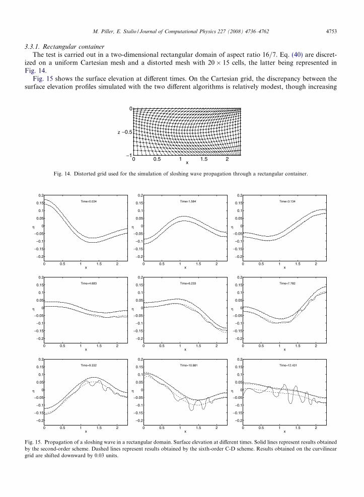
Since mechanical energy is expected to be globally conserved, the imbalance of mechanical energy EI,defined as the relative difference between the time-averaged and the instantaneous mechanical energy maybe as well used as an indicator of the quality of the results. Fig. 16 shows the evolution of EI obtained on boththe 20� 15 Cartesian and distorted meshes with the second-order and the sixth-order C-D schemes. While onthe Cartesian grid EI is always bounded, the poor quality of the second-order solution is confirmed on thedistorted grid where, unlike the C-D6 results, the imbalance tends to increase monotonically with time.

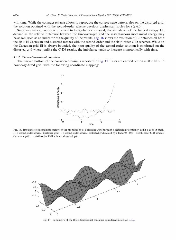
3.3.2. Three-dimensional container

The uneven bottom of the considered basin is reported in Fig. 17. Tests are carried out on a 30� 10� 15boundary-fitted grid, with the following coordinate mapping:

0 5 10 15−1

0

1

2

3

4

Mec

hani

cal E

nerg

y

time

Fig. 16. Imbalance of mechanical energy for the propagation of a sloshing wave through a rectangular container, using a 20 � 15 mesh.- - -: second-order scheme, Cartesian grid; –�–: second-order scheme, distorted grid (scaled by a factor 0.125); —: sixth-order C-D scheme,Cartesian grid; � � �: sixth-order C-D scheme, distorted grid.

0

0.5

1

1.5

2

0

0.2

0.4

−1.1

−1

−0.9

−0.8

Fig. 17. Bathimetry of the three-dimensional container considered in section 3.3.2.

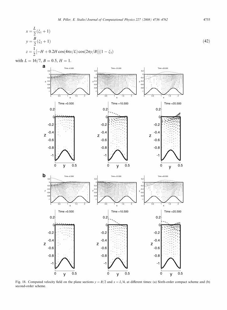
Fig. 18second


x ¼ L2ðn1 þ 1Þ

y ¼ B2ðn2 þ 1Þ

z ¼ 1

2½�H þ 0:2H cosð4px=LÞ cosð2py=BÞ�ð1� n3Þ

ð42Þ

with L ¼ 16=7, B ¼ 0:5, H ¼ 1.

. Computed velocity field on the plane sections y ¼ B=2 and x ¼ L=4, at different times: (a) Sixth-order compact scheme and (b)-order scheme.


Fig. 18 shows the computed velocity field on selected x–z and y–z planes, at different times. The free-surfaceelevation is also reported in the figure by a dashed line. Although the flow orientations predicted by the sec-ond-order and the sixth-order schemes are very similar, the compact scheme yields higher velocities at all con-sidered sections and times. Differences can also be observed for the computed surface elevation.

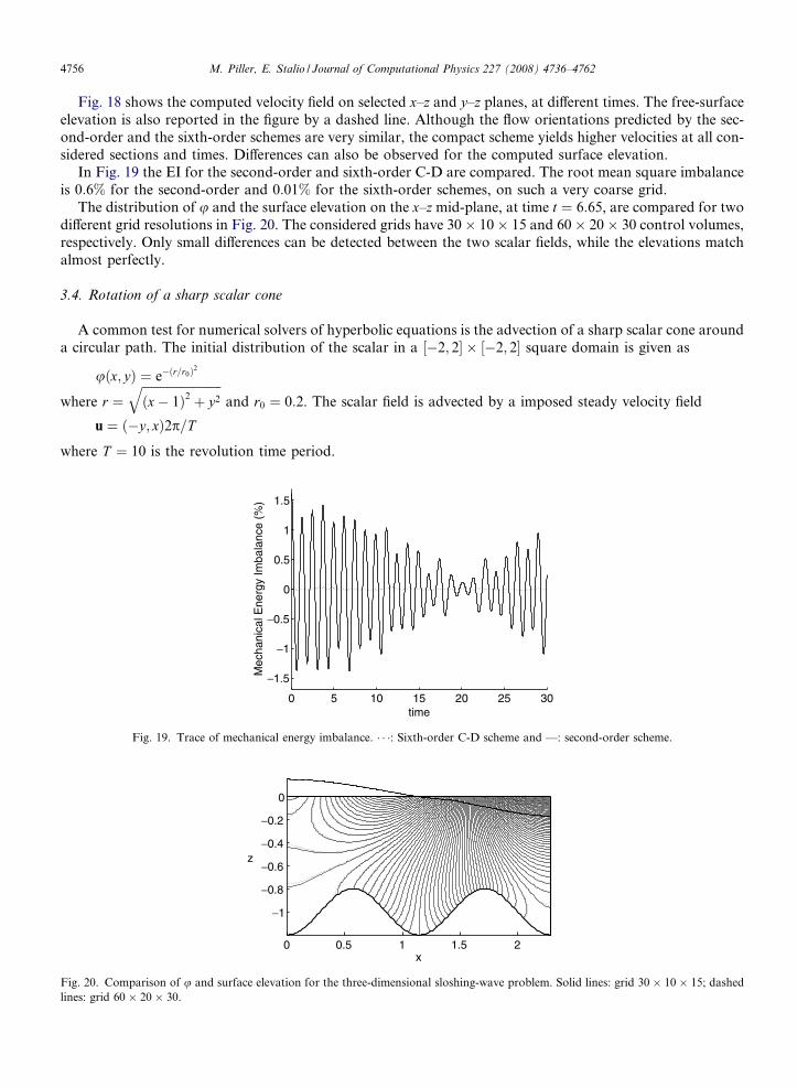
In Fig. 19 the EI for the second-order and sixth-order C-D are compared. The root mean square imbalanceis 0:6% for the second-order and 0:01% for the sixth-order schemes, on such a very coarse grid.

The distribution of u and the surface elevation on the x–z mid-plane, at time t ¼ 6:65, are compared for twodifferent grid resolutions in Fig. 20. The considered grids have 30� 10� 15 and 60� 20� 30 control volumes,respectively. Only small differences can be detected between the two scalar fields, while the elevations matchalmost perfectly.

3.4. Rotation of a sharp scalar cone

A common test for numerical solvers of hyperbolic equations is the advection of a sharp scalar cone arounda circular path. The initial distribution of the scalar in a ½�2; 2� � ½�2; 2� square domain is given as

Fig. 20lines: g

uðx; yÞ ¼ e�ðr=r0Þ2ffiffiffiffiffiffiffiffiffiffiffiffiffiffiffiffiffiffiffiffiffiffiffiffiffiffiq
where r ¼ ðx� 1Þ2 þ y2 and r0 ¼ 0:2. The scalar field is advected by a imposed steady velocity field
u ¼ ð�y; xÞ2p=T

where T ¼ 10 is the revolution time period.

0 0.5 1 1.5 2

−1

−0.8

−0.6

−0.4

−0.2

0

x

z

. Comparison of u and surface elevation for the three-dimensional sloshing-wave problem. Solid lines: grid 30 � 10 � 15; dashedrid 60 � 20 � 30.

0 5 10 15 20 25 30

−1.5

−1

−0.5

0

0.5

1

1.5

Mec

hani

cal E

nerg

y Im

bala

nce

(%)

time

Fig. 19. Trace of mechanical energy imbalance. � � �: Sixth-order C-D scheme and —: second-order scheme.


The coordinate mapping is defined as

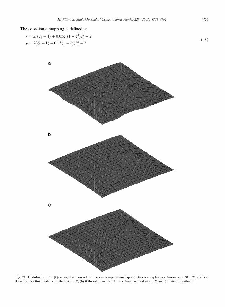
Fig. 21Second

x ¼ 2; ðn1 þ 1Þ þ 0:65n1ð1� n21Þn

22 � 2

y ¼ 2ðn2 þ 1Þ � 0:65ð1� n22Þn

21 � 2

ð43Þ

. Distribution of a u (averaged on control volumes in computational space) after a complete revolution on a 20 � 20 grid. (a)-order finite volume method at t ¼ T ; (b) fifth-order compact finite volume method at t ¼ T ; and (c) initial distribution.


Homogeneous Dirichlet boundary conditions are enforced at the cell faces located on inflow portions of theboundary, while there is no need to enforce outflow boundary conditions.

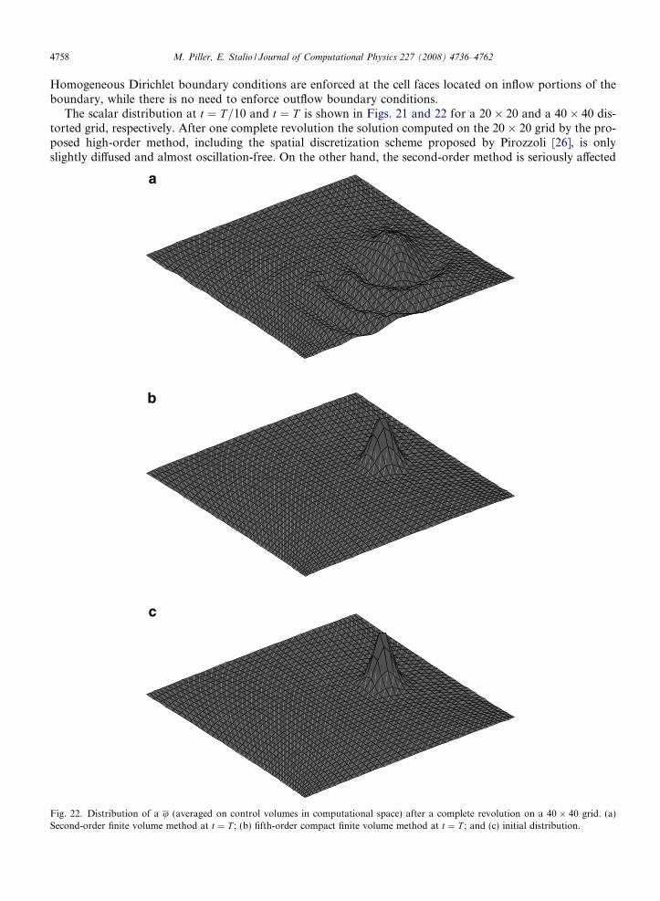
The scalar distribution at t ¼ T=10 and t ¼ T is shown in Figs. 21 and 22 for a 20� 20 and a 40� 40 dis-torted grid, respectively. After one complete revolution the solution computed on the 20� 20 grid by the pro-posed high-order method, including the spatial discretization scheme proposed by Pirozzoli [26], is onlyslightly diffused and almost oscillation-free. On the other hand, the second-order method is seriously affected

Fig. 22. Distribution of a u (averaged on control volumes in computational space) after a complete revolution on a 40 � 40 grid. (a)Second-order finite volume method at t ¼ T ; (b) fifth-order compact finite volume method at t ¼ T ; and (c) initial distribution.

0 0.2 0.4 0.6 0.8 1

10−4

10−2

t/T

εL

2

0.0 0.5 1.03.0

4.0

5.0

t/T

O(εL

2

)

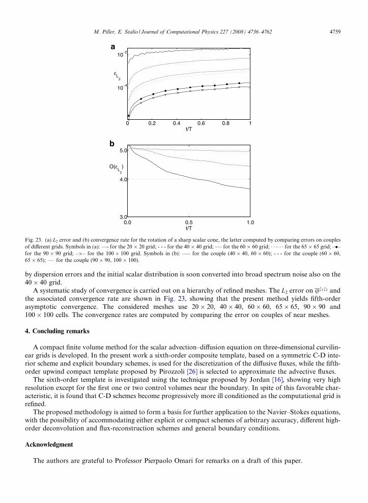
Fig. 23. (a) L2 error and (b) convergence rate for the rotation of a sharp scalar cone, the latter computed by comparing errors on couplesof different grids. Symbols in (a): —- for the 20 � 20 grid; - - - for the 40 � 40 grid; –�– for the 60 � 60 grid; � � �� for the 65 � 65 grid; ––for the 90 � 90 grid; –�– for the 100 � 100 grid. Symbols in (b): —– for the couple (40 � 40, 60 � 60); - - - for the couple (60 � 60,65 � 65); –�– for the couple (90 � 90, 100 � 100).


by dispersion errors and the initial scalar distribution is soon converted into broad spectrum noise also on the40� 40 grid.

A systematic study of convergence is carried out on a hierarchy of refined meshes. The L2 error on un1n2 andthe associated convergence rate are shown in Fig. 23, showing that the present method yields fifth-orderasymptotic convergence. The considered meshes use 20� 20, 40� 40, 60� 60, 65� 65, 90� 90 and100� 100 cells. The convergence rates are computed by comparing the error on couples of near meshes.

4. Concluding remarks

A compact finite volume method for the scalar advection–diffusion equation on three-dimensional curvilin-ear grids is developed. In the present work a sixth-order composite template, based on a symmetric C-D inte-rior scheme and explicit boundary schemes, is used for the discretization of the diffusive fluxes, while the fifth-order upwind compact template proposed by Pirozzoli [26] is selected to approximate the advective fluxes.

The sixth-order template is investigated using the technique proposed by Jordan [16], showing very highresolution except for the first one or two control volumes near the boundary. In spite of this favorable char-acteristic, it is found that C-D schemes become progressively more ill conditioned as the computational grid isrefined.

The proposed methodology is aimed to form a basis for further application to the Navier–Stokes equations,with the possibility of accommodating either explicit or compact schemes of arbitrary accuracy, different high-order deconvolution and flux-reconstruction schemes and general boundary conditions.

Acknowledgment

The authors are grateful to Professor Pierpaolo Omari for remarks on a draft of this paper.


Appendix A. Mathematical details of the Fourier analysis

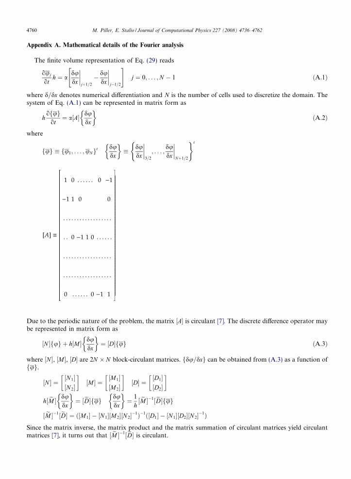
The finite volume representation of Eq. (29) reads

ouj

oth ¼ a

dudx

��jþ1=2

� dudx

��j�1=2

" #j ¼ 0; . . . ;N � 1 ðA:1Þ

where d=dx denotes numerical differentiation and N is the number of cells used to discretize the domain. Thesystem of Eq. (A.1) can be represented in matrix form as

hofug

ot¼ a½A� du

dx

� �ðA:2Þ

where

fug � fu1; . . . ;uNgt dudx

� �� du

dx

��3=2

; . . . ;dudx

��Nþ1=2

( )t

Due to the periodic nature of the problem, the matrix ½A� is circulant [7]. The discrete difference operator maybe represented in matrix form as

½N �fug þ h½M � dudx

� �¼ ½D� uf g ðA:3Þ

where ½N �, ½M �, ½D� are 2N � N block-circulant matrices. fdu=dxg can be obtained from (A.3) as a function offug.

½N � ¼½N 1�½N 2�

� �½M � ¼

½M1�½M2�

� �½D� ¼

½D1�½D2�

� �h½ eM � du

dx

� �¼ ½eD�fug du

dx

� �¼ 1

h½ eM ��1½eD�fug

½ eM ��1½eD� ¼ ð½M1� � ½N 1�½M2�½N 2��1Þ�1ð½D1� � ½N 1�½D2�½N 2��1Þ

Since the matrix inverse, the matrix product and the matrix summation of circulant matrices yield circulantmatrices [7], it turns out that ½ eM ��1½eD� is circulant.


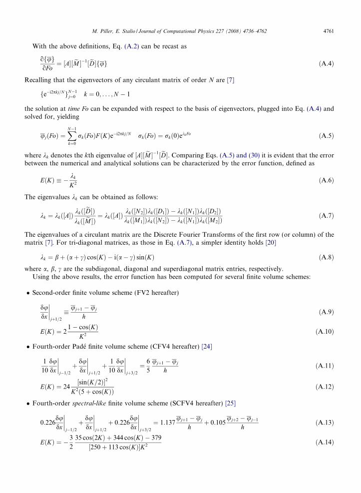
With the above definitions, Eq. (A.2) can be recast as

ofugoFo

¼ ½A�½ eM ��1½eD�fug ðA:4Þ

Recalling that the eigenvectors of any circulant matrix of order N are [7]

fe�i2pkj=NgN�1j¼0 k ¼ 0; . . . ;N � 1

the solution at time Fo can be expanded with respect to the basis of eigenvectors, plugged into Eq. (A.4) andsolved for, yielding

ujðFoÞ ¼XN�1

k¼0

rkðFoÞF ðKÞe�i2pkj=N rkðFoÞ ¼ rkð0Þekk Fo ðA:5Þ

where kk denotes the kth eigenvalue of ½A�½ eM ��1½eD�. Comparing Eqs. (A.5) and (30) it is evident that the errorbetween the numerical and analytical solutions can be characterized by the error function, defined as

EðKÞ � � kk

K2ðA:6Þ

The eigenvalues kk can be obtained as follows:

kk ¼ kkð½A�Þkkð½eD�Þkkð½ eM �Þ ¼ kkð½A�Þ

kkð½N 2�Þkkð½D1�Þ � kkð½N 1�Þkkð½D2�Þkkð½M1�Þkkð½N 2�Þ � kkð½N 1�Þkkð½M2�Þ

ðA:7Þ

The eigenvalues of a circulant matrix are the Discrete Fourier Transforms of the first row (or column) of thematrix [7]. For tri-diagonal matrices, as those in Eq. (A.7), a simpler identity holds [20]

kk ¼ bþ ðaþ cÞ cosðKÞ � iða� cÞ sinðKÞ ðA:8Þ
where a, b, c are the subdiagonal, diagonal and superdiagonal matrix entries, respectively.
Using the above results, the error function has been computed for several finite volume schemes:

Second-order finite volume scheme (FV2 hereafter)

dudx

��jþ1=2

� ujþ1 � uj

hðA:9Þ

EðKÞ ¼ 21� cosðKÞ

K2ðA:10Þ

Fourth-order Pade finite volume scheme (CFV4 hereafter) [24]

1

10

dudx

��j�1=2

þ dudx

��jþ1=2

þ 1

10

dudx

��jþ3=2

¼ 6

5

ujþ1 � uj

hðA:11Þ

EðKÞ ¼ 24½sinðK=2Þ�2

K2ð5þ cosðKÞÞðA:12Þ

Fourth-order spectral-like finite volume scheme (SCFV4 hereafter) [25]

0:226dudx

��j�1=2

þ dudx

��jþ1=2

þ 0:226dudx

��jþ3=2

¼ 1:137ujþ1 � uj

hþ 0:105

ujþ2 � uj�1

hðA:13Þ

EðKÞ ¼ � 3

2

35 cosð2KÞ þ 344 cosðKÞ � 379

½250þ 113 cosðKÞ�K2ðA:14Þ


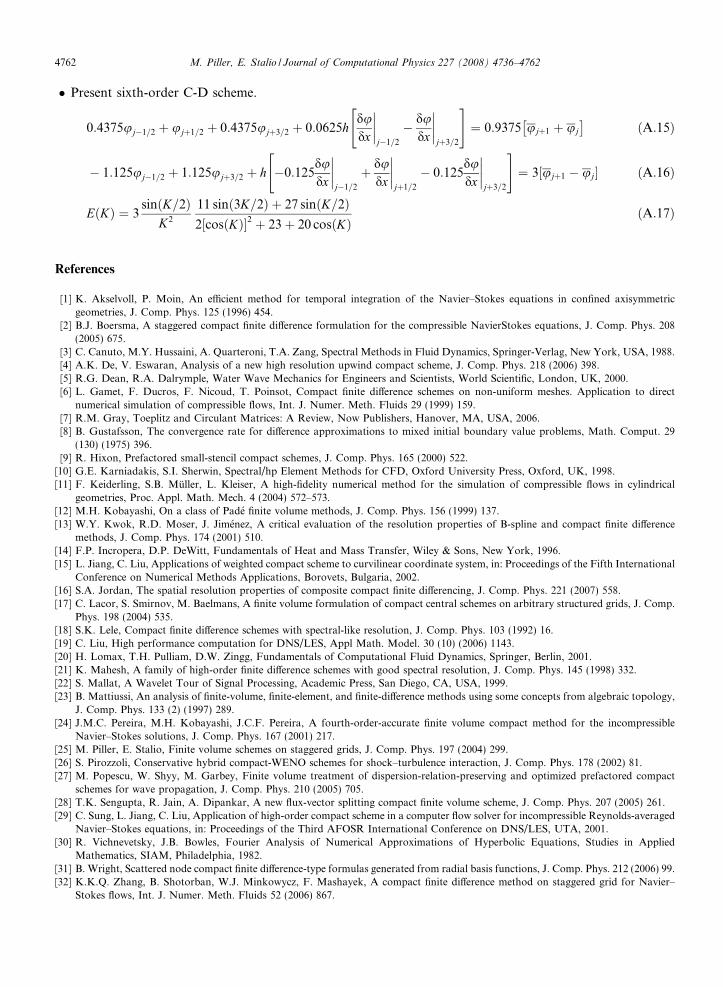
Present sixth-order C-D scheme.

0:4375uj�1=2 þ ujþ1=2 þ 0:4375ujþ3=2 þ 0:0625hdudx

��j�1=2

� dudx

��jþ3=2

" #¼ 0:9375 ujþ1 þ uj

�ðA:15Þ

� 1:125uj�1=2 þ 1:125ujþ3=2 þ h �0:125dudx

��j�1=2

þ dudx

��jþ1=2

� 0:125dudx

��jþ3=2

" #¼ 3½ujþ1 � uj� ðA:16Þ

EðKÞ ¼ 3sinðK=2Þ

K2

11 sinð3K=2Þ þ 27 sinðK=2Þ2½cosðKÞ�2 þ 23þ 20 cosðKÞ

ðA:17Þ

References

[1] K. Akselvoll, P. Moin, An efficient method for temporal integration of the Navier–Stokes equations in confined axisymmetricgeometries, J. Comp. Phys. 125 (1996) 454.

[2] B.J. Boersma, A staggered compact finite difference formulation for the compressible NavierStokes equations, J. Comp. Phys. 208(2005) 675.

[3] C. Canuto, M.Y. Hussaini, A. Quarteroni, T.A. Zang, Spectral Methods in Fluid Dynamics, Springer-Verlag, New York, USA, 1988.[4] A.K. De, V. Eswaran, Analysis of a new high resolution upwind compact scheme, J. Comp. Phys. 218 (2006) 398.[5] R.G. Dean, R.A. Dalrymple, Water Wave Mechanics for Engineers and Scientists, World Scientific, London, UK, 2000.[6] L. Gamet, F. Ducros, F. Nicoud, T. Poinsot, Compact finite difference schemes on non-uniform meshes. Application to direct

numerical simulation of compressible flows, Int. J. Numer. Meth. Fluids 29 (1999) 159.[7] R.M. Gray, Toeplitz and Circulant Matrices: A Review, Now Publishers, Hanover, MA, USA, 2006.[8] B. Gustafsson, The convergence rate for difference approximations to mixed initial boundary value problems, Math. Comput. 29

(130) (1975) 396.[9] R. Hixon, Prefactored small-stencil compact schemes, J. Comp. Phys. 165 (2000) 522.

[10] G.E. Karniadakis, S.I. Sherwin, Spectral/hp Element Methods for CFD, Oxford University Press, Oxford, UK, 1998.[11] F. Keiderling, S.B. Muller, L. Kleiser, A high-fidelity numerical method for the simulation of compressible flows in cylindrical

geometries, Proc. Appl. Math. Mech. 4 (2004) 572–573.[12] M.H. Kobayashi, On a class of Pade finite volume methods, J. Comp. Phys. 156 (1999) 137.[13] W.Y. Kwok, R.D. Moser, J. Jimenez, A critical evaluation of the resolution properties of B-spline and compact finite difference

methods, J. Comp. Phys. 174 (2001) 510.[14] F.P. Incropera, D.P. DeWitt, Fundamentals of Heat and Mass Transfer, Wiley & Sons, New York, 1996.[15] L. Jiang, C. Liu, Applications of weighted compact scheme to curvilinear coordinate system, in: Proceedings of the Fifth International

Conference on Numerical Methods Applications, Borovets, Bulgaria, 2002.[16] S.A. Jordan, The spatial resolution properties of composite compact finite differencing, J. Comp. Phys. 221 (2007) 558.[17] C. Lacor, S. Smirnov, M. Baelmans, A finite volume formulation of compact central schemes on arbitrary structured grids, J. Comp.

Phys. 198 (2004) 535.[18] S.K. Lele, Compact finite difference schemes with spectral-like resolution, J. Comp. Phys. 103 (1992) 16.[19] C. Liu, High performance computation for DNS/LES, Appl Math. Model. 30 (10) (2006) 1143.[20] H. Lomax, T.H. Pulliam, D.W. Zingg, Fundamentals of Computational Fluid Dynamics, Springer, Berlin, 2001.[21] K. Mahesh, A family of high-order finite difference schemes with good spectral resolution, J. Comp. Phys. 145 (1998) 332.[22] S. Mallat, A Wavelet Tour of Signal Processing, Academic Press, San Diego, CA, USA, 1999.[23] B. Mattiussi, An analysis of finite-volume, finite-element, and finite-difference methods using some concepts from algebraic topology,

J. Comp. Phys. 133 (2) (1997) 289.[24] J.M.C. Pereira, M.H. Kobayashi, J.C.F. Pereira, A fourth-order-accurate finite volume compact method for the incompressible

Navier–Stokes solutions, J. Comp. Phys. 167 (2001) 217.[25] M. Piller, E. Stalio, Finite volume schemes on staggered grids, J. Comp. Phys. 197 (2004) 299.[26] S. Pirozzoli, Conservative hybrid compact-WENO schemes for shock–turbulence interaction, J. Comp. Phys. 178 (2002) 81.[27] M. Popescu, W. Shyy, M. Garbey, Finite volume treatment of dispersion-relation-preserving and optimized prefactored compact

schemes for wave propagation, J. Comp. Phys. 210 (2005) 705.[28] T.K. Sengupta, R. Jain, A. Dipankar, A new flux-vector splitting compact finite volume scheme, J. Comp. Phys. 207 (2005) 261.[29] C. Sung, L. Jiang, C. Liu, Application of high-order compact scheme in a computer flow solver for incompressible Reynolds-averaged

Navier–Stokes equations, in: Proceedings of the Third AFOSR International Conference on DNS/LES, UTA, 2001.[30] R. Vichnevetsky, J.B. Bowles, Fourier Analysis of Numerical Approximations of Hyperbolic Equations, Studies in Applied

Mathematics, SIAM, Philadelphia, 1982.[31] B. Wright, Scattered node compact finite difference-type formulas generated from radial basis functions, J. Comp. Phys. 212 (2006) 99.[32] K.K.Q. Zhang, B. Shotorban, W.J. Minkowycz, F. Mashayek, A compact finite difference method on staggered grid for Navier–

Stokes flows, Int. J. Numer. Meth. Fluids 52 (2006) 867.

Compact finite volume schemes on boundary-fitted grids

Documents