High-order finite volume schemes on unstructured grids using moving least-squares reconstruction. Application to shallow water dynamics

INTERNATIONAL JOURNAL FOR NUMERICAL METHODS IN ENGINEERINGInt. J. Numer. Meth. Engng 2000; 00:1–6 Prepared using nmeauth.cls [Version: 2002/09/18 v2.02]

High order finite volume schemes on unstructured grids usingMoving Least Squares reconstruction. Application to shallow

water dynamics

L. Cueto-Felgueroso, I. Colominas∗, J. Fe, F. Navarrina, M. Casteleiro

Group of Numerical Methods in Engineering, GMNIDept. of Applied Mathematics, Civil Engineering School

Universidad de La CorunaCampus de Elvina, 15071 La Coruna, SPAIN

SUMMARY

This paper introduces the use of Moving Least Squares (MLS) approximations for the developmentof high-order finite volume discretizations on unstructured grids. The field variables and theirsuccesive derivatives can be accurately reconstructed using this meshfree technique in a generalnodal arrangement. The methodology proposed is used in the construction of low-dissipative high-order high-resolution schemes for the shallow water equations. In particular, second and third-order-reconstruction upwind schemes for unstructured grids based on Roe’s flux difference splitting aredeveloped and applied to inviscid and viscous flows. This class of meshfree reconstruction techniquesprovide a robust and general approximation framework which represents an interesting alternative tothe existing procedures, allowing, in addition, an accurate computation of the viscous fluxes. Copyrightc© 2000 John Wiley & Sons, Ltd.

key words: Shallow Water dynamics, Finite Volume method, high-resolution schemes, meshfree

methods, Moving Least-Squares, unstructured grids.

1. INTRODUCTION

The development of a general algorithm capable of achieving optimal performance in all flowproblems is one of the most important and challenging areas of research in ComputationalMechanics. In the context of shallow water dynamics, finite element and finite volumediscretizations have become very popular in recent years.

Finite element formulations for fluid dynamics are usually elegant and applicable to awide variety of flow conditions. Unfortunately, their frequent centered character hinderstheir suitability for problems involving shock waves and transcritical flow, thus requiring thedevelopment and tuning of more or less effective artificial viscosity models. One of the most

∗Correspondence to: E.T.S. de Ingenieros de Caminos, Canales y Puertos, Universidad de La Coruna, Campusde Elvina, 15071 La Coruna, SPAIN. Email: [email protected]

Received YesterdayCopyright c© 2000 John Wiley & Sons, Ltd. Revised Today

2 L. CUETO-FELGUEROSO, I. COLOMINAS, J. FE, F. NAVARRINA, M. CASTELEIRO

succesful of these finite element schemes applied to the shallow water equations is the Taylor-Galerkin FEM algorithm proposed by Peraire [1],[2], which has been further developed byQuecedo and Pastor [3], [4]. Sheu and Fang [5] have recently proposed a generalized Taylor-Galerkin finite element method to obtain high resolution of discontinuous flows.

Most finite volume formulations for the set of shallow water equations are reflections of highresolution schemes originally devised to solve high speed compressible flows, and have beensuccesfully employed in the simulation of flows including the presence of shock waves, such asbreaking dams or hydraulic jumps, almost invariably neglecting viscous and turbulent effects.Alcrudo and Garcıa-Navarro [6] developed a Godunov-type MUSCL high-resolution schemebased on Roe’s Riemann solver. Zhao et al. [7] proposed an upwind finite volume methodon unstructured grids using Osher’s scheme. Anastasiou and Chan [8] solved the full set ofshallow water equations on unstructured meshes using a second order Roe scheme and reportedresults for viscous flows at low Reynolds numbers. Other upwind schemes with shock-capturingcapabilities have been proposed by Hu and Mingham [9] and Tseng [10]. Liszka and Wendroff[11] introduced composite methods, which combine Lax-Wendroff and Lax-Friedrichs schemesinto a multistage algorithm, and Wang and Liu [12] have recently extended the methodologyto unstructured triangular meshes.

Various researchers have reported that first and even second order upwind schemes exhibitexcessive numerical dissipation when applied to more general flows (not necessarily includingshock wave propagation) where turbulent effects are of interest [13],[14],[15], and severalcorrections to the original algorithms have been proposed in order to reduce the unnecessaryartificial dissipation introduced in the computations. Unfortunately, these corrections aresomewhat “heuristic”, and yet remains a compromise between accuracy and stability: the lesserthe dissipation added the more accurate the results, whereas some amount of artificial viscosityis unavoidably necessary to yield stable algorithms. A suitable numerical method to solvesuch problems on unstructured meshes should therefore not introduce exccessive numericaldissipation, in order to capture fine viscous features of the flow and to avoid interactions withthe turbulence model. Furthermore, when shock wave-turbulence interactions are present inthe flow, the numerical method should possess the low dissipation of high order methods andthe shock capturing capabilities of Godunov-type schemes [16].

The endeavour to solve increasingly complex flows has promoted the advent of unstructuredmeshes as the most efficient approach to mesh highly irregular domains, perform adaptiverefinements and capture small scale features of the flow. As far as the development ofhigh order finite volume schemes for unstructured meshes is concerned, the absence of anunderlying spatial approximation framework, which stems from the inherent piecewise constantrepresentation, is certainly a most challenging algorithmic issue. Most schemes are at bestsecond order and even the required reconstruction of fluxes and gradients is addressed by usingsomewhat “heuristic” techniques, which frequently lead to quite complex data processing whenproper accuracy and low grid sensitivity are pursued.

The authors would like to propose a meshfree technique, the so-called Moving Least Squares(MLS) approximation as an accurate and efficient technique to obtain high order finite volumealgorithms on unstructered meshes. This class of approximation methods is particularly wellsuited for such purpose, providing a robust and general approximation framework whichrepresents an interesting alternative to the existing techniques, and allowing, in addition,an accurate computation of the viscous fluxes. Originally devised for data processing [17],the MLS approximation has become very popular among those researchers working in the

Copyright c© 2000 John Wiley & Sons, Ltd. Int. J. Numer. Meth. Engng 2000; 00:1–6Prepared using nmeauth.cls

HIGH ORDER FV SCHEMES USING MLS RECONSTRUCTION 3

class of the so-called meshless or meshfree methods, being widely used both in eulerian andlagrangian formulations. In particular, the authors have recently proposed an algorithm forlagrangian particle hydrodynamics, where the MLS technique played a key role to provide thespatial approximation within an arbitrary cloud of nodes [18]. In this study, second and third-order-reconstruction high-resolution schemes, based on Roe’s approximate Riemann solver[19], are developed and tested for inviscid and viscous flow applications. In the latter, theapproximation framework provided by these meshfree techniques is especially interesting inthe accurate evaluation of the viscous fluxes at the cell faces. Although further work focusedon adequate limiting strategies is neccesary to exploit the whole capabilities of the third-orderscheme in problems with strong shocks, the preliminary results are encouraging.

For comparison purposes, particularly in the case os viscous flow, a Lax-Wendroff finitevolume scheme was also implemented and tested on unstructered grids. In this case, we usedagain the MLS shape functions to obtain a continuous representation of the field variablesand their derivatives within the grid. This Lax-Wendroff scheme is not free from spuriousoscillations that may undermine the solution in the presence of shocks. An artificial viscositymodel is proposed, in complete analogy to those used in the finite element literature for highspeed compressible flows. The resulting scheme possesses accuracy and stability propertiesvery similar to its finite element counterpart, the Taylor-Galerkin FEM, and can be appliedto a wide variety of problems of engineering interest, particularly when viscous and turbulenteffects are of the utmost importance.

The outline of the paper is as follows. Section 2 presents a brief introduction to some meshlessapproximation techniques, with special emphasis on Moving Least Squares and ReproducingKernel methods. The model equations and numerical formulations employed in this study arediscussed in section 3. Finally, section 4 is devoted to numerical examples and other practicalimplementation issues.

2. MESHLESS APPROXIMATION: MOVING LEAST SQUARES

2.1. The idea of a meshfree interpolation.

The endeavour to solve the continuum equations in a particle (as opposed to cell or element)framework, i.e. simply using the information stored at certain nodes or particles withoutreference to any underlying mesh, has given rise to a very active area of research: the class ofso-called meshless, meshfree or particle methods.

If this particle approach is to be used in combination with classical discretization procedures(e.g. the weighted residuals method), then a spatial approximation is required (some kind of“shape functions”, as in the finite element method). Such an interpolation scheme shouldaccurately reproduce or reconstruct a certain function and its succesive derivatives using thenodal (particle) values and some “low-level” geometrical information about the grid, such asthe distance between particles. Furthermore, and in order to achieve computationally efficientalgorithms, the interpolation should have a local character, i.e. the reconstruction processshould involve only a few “neighbour” nodes.

Even though a “perfect” meshless approximation scheme, capable of achieving high accuracyfor any randomly distributed set of points, is still not available, several powerful interpolationtechniques have been recently proposed, thus enabling the development of increasingly efficient



and accurate meshless formulations. What follows is a brief introduction to a certain classof such interpolation schemes, namely those based on reproducing kernel and moving leastsquares approximations. Further emphasis is placed on the particular technique used in thisstudy, although the reader is referred to the classical meshfree literature to find in depthdescriptions of these algorithms.

2.2. Meshless approximants.

The origin of modern meshless methods could be dated back to the 70’s with the pioneeringworks in generalized finite differences and vortex particle methods [20],[21],[22]. However, thestrongest influence upon the present trends is commonly attributed to early Smoothed ParticleHydrodynamics (SPH) formulations [23],[24],[25], where a lagrangian particle tracking is usedto describe the motion of a fluid. Although this general feature is shared with vortex particlemethods, SPH includes a spatial approximation framework (some kind of “meshfree shapefunctions”), developed using the concept of kernel estimate, which is inspired by the followingproperty of the Dirac delta function

u(xxxxxxxxxxxxxx) =∫

yyyyyyyyyyyyyy∈Ω

u(yyyyyyyyyyyyyy)δ(xxxxxxxxxxxxxx− yyyyyyyyyyyyyy)dΩ (1)

The kernel estimate 〈u(xxxxxxxxxxxxxx)〉 of a given function u(xxxxxxxxxxxxxx) is defined as

〈u(xxxxxxxxxxxxxx)〉 =∫

yyyyyyyyyyyyyy∈Ω

u(yyyyyyyyyyyyyy)W (xxxxxxxxxxxxxx− yyyyyyyyyyyyyy, ρ)dΩ (2)

and its discrete SPH counterpart u(xxxxxxxxxxxxxx) is

u(xxxxxxxxxxxxxx) =n∑

j=1

ujW (xxxxxxxxxxxxxx− xxxxxxxxxxxxxxj , ρ)Vj (3)

where Ω is the problem domain, which is discretized into a set of n nodes or particles (used asquadrature points in (2)), W (xxxxxxxxxxxxxx−xxxxxxxxxxxxxxj , ρ) is a kernel (smoothing) function with compact supportcentered at particle j and Vj is the tributary or statistical “volume” associated to particlej. The parameter ρ, usually called smoothing length or dilation parameter in the meshfreeliterature, is a certain characteristic measure of the size of the support of Wj (e.g. kernels withcircular supports of radius 2ρ). Exponential and spline funtions are most frequent kernels. Inanalogy with the finite element method, the approximation (3) could be cast in terms of SPH“shape functions”, as

u(xxxxxxxxxxxxxx) =n∑

j=1

ujNj(xxxxxxxxxxxxxx), Nj(xxxxxxxxxxxxxx) = W (xxxxxxxxxxxxxx− xxxxxxxxxxxxxxj , ρ)Vj (4)

Using standard kernels, the aproximation given by (4) is poor near boundaries, and lacks evenzeroth order completeness, i.e.

n∑

j=1

Nj(xxxxxxxxxxxxxx) 6= 1 (5)



The gradient of u(xxxxxxxxxxxxxx) is evaluated as

∇∇∇∇∇∇∇∇∇∇∇∇∇∇xxxxxxxxxxxxxxu(xxxxxxxxxxxxxx) =n∑

j=1

uj∇∇∇∇∇∇∇∇∇∇∇∇∇∇xxxxxxxxxxxxxxNj(xxxxxxxxxxxxxx) =n∑

j=1

uj∇∇∇∇∇∇∇∇∇∇∇∇∇∇xxxxxxxxxxxxxxWj(xxxxxxxxxxxxxx)Vj (6)

In practice, alternative expressions for ∇∇∇∇∇∇∇∇∇∇∇∇∇∇xxxxxxxxxxxxxxu(xxxxxxxxxxxxxx) are frequent in the SPH literature to enforceconservation properties in the discrete equations. Higher order derivatives could be computedin a similar fashion. Note that the reconstructed values of u(xxxxxxxxxxxxxx) and its derivatives at a certainlocation are obtained using the information from neighbouring nodes and weightings that arefunctions of distances between nodes, with no reference to any mesh-based data structure(Figure 1).

Figure 1. Meshfree approximation: general scheme. Support for reconstruction at P.

This basic approximation structure is retained in other improved interpolation schemes.In this study only Moving Least Squares (MLS) and Reproducing Kernel Particle (RKPM)methods are considered. Although different in their formulation, the resulting numerics arealmost identical for both methods, and they can be presented within a common approach.

Let us consider a function u(xxxxxxxxxxxxxx) defined in a bounded, or unbounded, domain Ω. The basicidea of the MLS approach is to approximate u(xxxxxxxxxxxxxx), at a given point xxxxxxxxxxxxxx, through a polynomialleast-squares fitting of u(xxxxxxxxxxxxxx) in a neighbourhood of xxxxxxxxxxxxxx as

u(xxxxxxxxxxxxxx) ≈ u(xxxxxxxxxxxxxx) =m∑

i=1

pi(xxxxxxxxxxxxxx)αi(zzzzzzzzzzzzzz)∣∣∣zzzzzzzzzzzzzz=xxxxxxxxxxxxxx

= ppppppppppppppT (xxxxxxxxxxxxxx)αααααααααααααα(zzzzzzzzzzzzzz)∣∣∣zzzzzzzzzzzzzz=xxxxxxxxxxxxxx

(7)

where ppppppppppppppT (xxxxxxxxxxxxxx) is an m-dimensional polynomial basis and αααααααααααααα(zzzzzzzzzzzzzz)∣∣∣zzzzzzzzzzzzzz=xxxxxxxxxxxxxx

is a set of parameters to bedetermined, such that they minimize the following error functional



J(αααααααααααααα(zzzzzzzzzzzzzz)∣∣∣zzzzzzzzzzzzzz=xxxxxxxxxxxxxx

) =∫

yyyyyyyyyyyyyy∈ΩxxxxxxxxxxxxxxW (zzzzzzzzzzzzzz − yyyyyyyyyyyyyy, ρ)

∣∣∣zzzzzzzzzzzzzz=xxxxxxxxxxxxxx

[u(yyyyyyyyyyyyyy)− ppppppppppppppT (yyyyyyyyyyyyyy)αααααααααααααα(zzzzzzzzzzzzzz)


]2

dΩxxxxxxxxxxxxxx (8)

being W (zzzzzzzzzzzzzz− yyyyyyyyyyyyyy, ρ)∣∣∣zzzzzzzzzzzzzz=xxxxxxxxxxxxxx

a symmetric kernel with compact support (denoted by Ωxxxxxxxxxxxxxx), frequentlychosen among the kernels used in standard SPH. As mentioned before, ρ is the smoothinglength, which measures the size of Ωxxxxxxxxxxxxxx. The stationary conditions of J with respect to αααααααααααααα leadto

∫

yyyyyyyyyyyyyy∈Ωxxxxxxxxxxxxxxpppppppppppppp(yyyyyyyyyyyyyy)W (zzzzzzzzzzzzzz − yyyyyyyyyyyyyy, ρ)


u(yyyyyyyyyyyyyy)dΩxxxxxxxxxxxxxx = MMMMMMMMMMMMMM(xxxxxxxxxxxxxx)αααααααααααααα(zzzzzzzzzzzzzz)∣∣∣zzzzzzzzzzzzzz=xxxxxxxxxxxxxx

(9)

where the moment matrix MMMMMMMMMMMMMM(xxxxxxxxxxxxxx) is

MMMMMMMMMMMMMM(xxxxxxxxxxxxxx) =∫

yyyyyyyyyyyyyy∈Ωxxxxxxxxxxxxxxpppppppppppppp(yyyyyyyyyyyyyy)W (zzzzzzzzzzzzzz − yyyyyyyyyyyyyy, ρ)


ppppppppppppppT (yyyyyyyyyyyyyy)dΩxxxxxxxxxxxxxx (10)

In numerical computations, the global domain Ω is discretized by a set of n particles. Wecan then evaluate the integrals in (9) and (10) using those particles inside Ωxxxxxxxxxxxxxx as quadraturepoints (nodal integration) to obtain, after rearranging,

αααααααααααααα(zzzzzzzzzzzzzz)∣∣∣zzzzzzzzzzzzzz=xxxxxxxxxxxxxx

= MMMMMMMMMMMMMM−1(xxxxxxxxxxxxxx)PPPPPPPPPPPPPPΩxxxxxxxxxxxxxxWWWWWWWWWWWWWWV (xxxxxxxxxxxxxx)uuuuuuuuuuuuuuΩxxxxxxxxxxxxxx (11)

where the vector uuuuuuuuuuuuuuΩxxxxxxxxxxxxxx contains certain nodal parameters of those particles in Ωxxxxxxxxxxxxxx, the discreteversion of M is M(xxxxxxxxxxxxxx) = PΩxxxxxxxxxxxxxxWV(xxxxxxxxxxxxxx)PT

Ωxxxxxxxxxxxxxx , and matrices PΩxxxxxxxxxxxxxx and WV(xxxxxxxxxxxxxx) can be obtained as

PPPPPPPPPPPPPPΩxxxxxxxxxxxxxx =(pppppppppppppp(xxxxxxxxxxxxxx1) pppppppppppppp(xxxxxxxxxxxxxx2) · · · pppppppppppppp(xxxxxxxxxxxxxxnxxxxxxxxxxxxxx)

)(12)

WV(xxxxxxxxxxxxxx) = diag Wi(xxxxxxxxxxxxxx− xxxxxxxxxxxxxxi)Vi , i = 1, . . . , nxxxxxxxxxxxxxx (13)

Complete details can be found in [26], [27], [28]. In the above equations, nxxxxxxxxxxxxxx denotes the totalnumber of particles within the neighbourhood of point xxxxxxxxxxxxxx and Vi and xxxxxxxxxxxxxxi are, respectively, thetributary volume (used as quadrature weight) and coordinates associated to particle i. Notethat the tributary volumes of neighbouring particles are included in matrix WV, obtainingan MLS version of the Reproducing Kernel Particle Method (the so-called MLSRKPM) [26].Otherwise, we can use W instead of WV

W(xxxxxxxxxxxxxx) = diag Wi(xxxxxxxxxxxxxx− xxxxxxxxxxxxxxi) , i = 1, . . . , nxxxxxxxxxxxxxx (14)

which corresponds to the classical MLS approximation (in the nodal integration of thefunctional (8), the same quadrature weight is associated to all particles). Introducing (11)in (7) the interpolation structure can be identified as

u(xxxxxxxxxxxxxx) = ppppppppppppppT (xxxxxxxxxxxxxx)MMMMMMMMMMMMMM−1(xxxxxxxxxxxxxx)PPPPPPPPPPPPPPΩxxxxxxxxxxxxxxWWWWWWWWWWWWWWV (xxxxxxxxxxxxxx)uuuuuuuuuuuuuuΩxxxxxxxxxxxxxx = NNNNNNNNNNNNNNT (xxxxxxxxxxxxxx)uuuuuuuuuuuuuuΩxxxxxxxxxxxxxx (15)

And, therefore, the MLS shape functions can be written as

NNNNNNNNNNNNNNT (xxxxxxxxxxxxxx) = ppppppppppppppT (xxxxxxxxxxxxxx)MMMMMMMMMMMMMM−1(xxxxxxxxxxxxxx)PPPPPPPPPPPPPPΩxxxxxxxxxxxxxxWWWWWWWWWWWWWWV (xxxxxxxxxxxxxx) (16)



It is most frequent to use a scaled and locally defined polinomial basis, instead of the globallydefined pppppppppppppp(yyyyyyyyyyyyyy). Thus, if the shape functions are to be evaluated at point xxxxxxxxxxxxxx, the basis would beof the form pppppppppppppp(yyyyyyyyyyyyyy−xxxxxxxxxxxxxx

ρ ). The shape functions are, therefore, of the form

NNNNNNNNNNNNNNT (xxxxxxxxxxxxxx) = ppppppppppppppT (00000000000000)CCCCCCCCCCCCCC(xxxxxxxxxxxxxx) = ppppppppppppppT (00000000000000)MMMMMMMMMMMMMM−1(xxxxxxxxxxxxxx)PPPPPPPPPPPPPPΩxxxxxxxxxxxxxxWWWWWWWWWWWWWWV (xxxxxxxxxxxxxx) (17)

Their first derivatives could be computed as

∂NNNNNNNNNNNNNNT (xxxxxxxxxxxxxx)∂xi

=∂ppppppppppppppT (00000000000000)

∂xiCCCCCCCCCCCCCC(xxxxxxxxxxxxxx) + ppppppppppppppT (00000000000000)

∂CCCCCCCCCCCCCC(xxxxxxxxxxxxxx)∂xi

(18)

where

∂CCCCCCCCCCCCCC(xxxxxxxxxxxxxx)∂xi

= CCCCCCCCCCCCCC(xxxxxxxxxxxxxx)WWWWWWWWWWWWWW−1(xxxxxxxxxxxxxx)∂WWWWWWWWWWWWWW (xxxxxxxxxxxxxx)

∂xi

(IIIIIIIIIIIIII − PPPPPPPPPPPPPPT

ΩxxxxxxxxxxxxxxCCCCCCCCCCCCCC(xxxxxxxxxxxxxx))

(19)

and expressions for higher order derivatives could be analogously obtained. Fast algorithms toperform these computations have been proposed [20],[29]. Examples of 2D basis functions arethe quadratic polinomial basis

pppppppppppppp(yyyyyyyyyyyyyy − xxxxxxxxxxxxxx

ρ) =

(1, z1, z2, z1z2, z

21 , z2

2

)(20)

which provides quadratic completeness, and the cubic basis

pppppppppppppp(yyyyyyyyyyyyyy − xxxxxxxxxxxxxx

ρ) =

(1, z1, z2, z1z2, z

21 , z2

2 , z21z2, z1z

22 , z3

1 , z32

)(21)

for cubic completeness. In the above equations, zi = (yi − xi)/ρ, and (x1, x2) and (y1, y2)are, respectively, the cartesian coordinates of xxxxxxxxxxxxxx and yyyyyyyyyyyyyy. The concept of completeness alludesto the ability of the scheme to exactly reproduce polinomials and its derivatives. Thus, if thequadratic basis (20) is used, the approximation verifies

n∑

j=1

xaj yb

jNj(xxxxxxxxxxxxxx) = xayb, a ≥ 0, b ≥ 0, a + b ≤ 2 (22)

n∑

j=1

xaj yb

j

∂Nj(xxxxxxxxxxxxxx)∂x

= axa−1yb, a ≥ 0, b ≥ 0, a + b ≤ 2 (23)

n∑

j=1

xaj yb

j

∂Nj(xxxxxxxxxxxxxx)∂y

= bxayb−1, a ≥ 0, b ≥ 0, a + b ≤ 2 (24)

and so on. In general, any linear combination of the functions included in the basis pppppppppppppp(yyyyyyyyyyyyyy−xxxxxxxxxxxxxxρ ) is

exactly reproduced by the MLS approximation.A wide variety of kernel functions appear in the literature, most of them being spline or

exponential functions. In this study we use a very popular cubic spline

Wj(xxxxxxxxxxxxxx) = W (xxxxxxxxxxxxxx− xxxxxxxxxxxxxxj , ρ) =α

ρν

1− 32s2 + 3

4s3 s ≤ 114 (2− s)3 1 < s ≤ 20 s > 2

(25)



where s = ‖xxxxxxxxxxxxxx− xxxxxxxxxxxxxxj‖ρ , ν is the number of dimensions and α takes the value 2

3 , 107π or 1

π in one,two or three dimensions, respectively. The coeficient α/ρν is a scale factor neccesary only ifnon-corrected SPH interpolation is being used, to assure the normality property

∫WdV = 1.

We do not use it in our MLS computations. Anisotropic weightings (with rectangular insteadof circular supports) for 2D/3D computations can be constructed as tensor-product of one-dimensional kernels as

Wj(xxxxxxxxxxxxxx− xxxxxxxxxxxxxxj , ρ) =ν∏

n=1

Wnj (xn − xn

j , ρn) (26)

where xn is the n-th coordinate of particle xxxxxxxxxxxxxx. In the above expression we let Wnj and ρn (the

one-dimensional kernel function and its caracteristic smoothing length) be different for eachspatial dimension.

2.3. Computational aspects. Application to finite volume procedures.

The technique exposed above provides a general approximation framework which can be usedin combination with existing finite volume methods. The field variables and their succesivederivatives are reconstructed at certain evaluation points (usually face midpoints or cellcenters) using the cell-average information, customarily associated to the cell centers, which aretaken here as the nodes or particles of the meshfree aproximation scheme. The reconstructioninvolves three major steps:

• Determine the “neighbourhood” of the evaluation point, i.e. which nodes (cell-centers)contribute to the reconstruction process.

• Compute the MLS shape functions and their required derivatives at the evaluation point,as exposed in section 2.2.

• Compute the approximate value of the field variables an their succesive derivatives usingthe general expressions

u(xxxxxxxxxxxxxx) =nxxxxxxxxxxxxxx∑

j=1

ujNj(xxxxxxxxxxxxxx),∂αu(xxxxxxxxxxxxxx)

∂xαk

=nxxxxxxxxxxxxxx∑

j=1

uj∂αNj(xxxxxxxxxxxxxx)

∂xαk

(27)

being nxxxxxxxxxxxxxx the number of neighbouring cell-centers whose field values uj are used in thereconstruction.

Note that, if a time marching scheme is to be used, the two first steps can be included in thepreprocessing phase, as the MLS shape functions do not change in time for a fixed grid.

2.3.1. Cost and algorithmic complexity. The computation of the MLS shape functions is anexpensive task if compared, for instance, to the FEM shape functions. However, and for agiven finite volume mesh, where the information is stored at cell-centers, the shape functionsand their derivatives need to be computed only once, at the beginning of the simulation. Thetime spent in such task is then negligible if compared to the whole simulation time. On theother hand, the evaluation of gradients and, eventually, other interpolated values at each timestep becomes an extremely simple process, using the general expressions (27). In particular



u(xxxxxxxxxxxxxx) =nxxxxxxxxxxxxxx∑

j=1

ujNj(xxxxxxxxxxxxxx), ∇∇∇∇∇∇∇∇∇∇∇∇∇∇u(xxxxxxxxxxxxxx) =nxxxxxxxxxxxxxx∑

j=1

uj∇∇∇∇∇∇∇∇∇∇∇∇∇∇Nj(xxxxxxxxxxxxxx) (28)

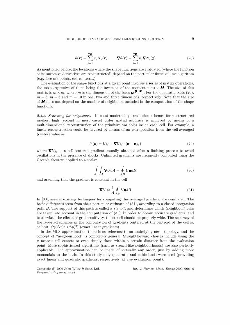
As mentioned before, the locations where the shape functions are evaluated (where the functionor its succesive derivatives are reconstructed) depend on the particular finite volume algorithm(e.g. face midpoints, cell-centers...).

The evaluation of the shape functions at a given point involves a series of matrix operations,the most expensive of them being the inversion of the moment matrix MMMMMMMMMMMMMM . The size of thismatrix is m×m, where m is the dimension of the basis pppppppppppppp(yyyyyyyyyyyyyy−xxxxxxxxxxxxxx

ρ ). For the quadratic basis (20),m = 3, m = 6 and m = 10 in one, two and three dimensions, respectively. Note that the sizeof MMMMMMMMMMMMMM does not depend on the number of neighbours included in the computation of the shapefunctions.

2.3.2. Searching for neighbours. In most modern high-resolution schemes for unstructuredmeshes, high (second in most cases) order spatial accuracy is achieved by means of amultidimensional reconstruction of the primitive variables inside each cell. For example, alinear reconstruction could be devised by means of an extrapolation from the cell-averaged(center) value as

U(xxxxxxxxxxxxxx) = UM +∇∇∇∇∇∇∇∇∇∇∇∇∇∇UM · (xxxxxxxxxxxxxx− xxxxxxxxxxxxxxM ) (29)

where ∇∇∇∇∇∇∇∇∇∇∇∇∇∇UM is a cell-centered gradient, usually obtained after a limiting process to avoidoscillations in the presence of shocks. Unlimited gradients are frequently computed using theGreen’s theorem applied to a scalar

∫ ∫

A

∇∇∇∇∇∇∇∇∇∇∇∇∇∇UdA =∮

B

UnnnnnnnnnnnnnndB (30)

and assuming that the gradient is constant in the cell

∇∇∇∇∇∇∇∇∇∇∇∇∇∇U ≈ 1A

∮

B

UnnnnnnnnnnnnnndB (31)

In [30], several existing techniques for computing this averaged gradient are compared. Thebasic differences stem from their particular estimate of (31), according to a closed integrationpath B. The support of this path is called a stencil , and determines which (neighbour) cellsare taken into account in the computation of (31). In order to obtain accurate gradients, andto alleviate the effects of grid sensitivity, the stencil should be properly wide. The accuracy ofthe reported schemes in the computation of gradients centered at the centroid of the cell is,at best, O((∆x)2, (∆y)2) (exact linear gradients).

In the MLS approximation there is no reference to an underlying mesh topology, and theconcept of “neigbourhood” is completely general. Straightforward choices include using then nearest cell centers or even simply those within a certain distance from the evaluationpoint. More sophisticated algorithms (such as stencil-like neighbourhoods) are also perfectlyapplicable. The approximation can be made of virtually any order, just by adding moremonomials to the basis. In this study only quadratic and cubic basis were used (providingexact linear and quadratic gradients, respectively, at any evaluation point).



Nevertheless, the cloud of neighbours must verify certain “minimum” requirements, whichare mainly related to the inversion of the moment matrix MMMMMMMMMMMMMM . If the number of neighboursis less than m (the number of functions in the basis), MMMMMMMMMMMMMM becomes singular, which impliesthat more than 6 neighbours are needed in 2D computations with the quadratic basis. Ingeneral, the approximation could be poor if MMMMMMMMMMMMMM is highly ill-conditioned, so it is convenient touse a number of neighbours greater than the minimum, and with information coming fromall possible directions. We have used 14 − −16 neighbours in the 2D examples shown in thisstudy.

2.3.3. Diffuse derivatives. The concept of diffuse derivative is very interesting from acomputational point of view in MLS approximations. In the diffuse approach, the derivativesof the shape functions are approximated by the first term in (18) as

∂NNNNNNNNNNNNNNT (xxxxxxxxxxxxxx)∂xi

≈ ∂ppppppppppppppT (00000000000000)∂xi

CCCCCCCCCCCCCC(xxxxxxxxxxxxxx) (32)

It has been shown (see [31] and references therein) that the diffuse derivatives of a functionu(xxxxxxxxxxxxxx), given by

∂u(xxxxxxxxxxxxxx)∂xi

≈nxxxxxxxxxxxxxx∑

j=1

uj∂Nj(xxxxxxxxxxxxxx)

∂xi(33)

converge at optimal rate to the exact derivatives. The same procedure can be extended to thesuccesive derivatives of u(xxxxxxxxxxxxxx). The fact that the order of the approximation is preserved andthe much simpler numerics required in the computation of diffuse derivatives will be exploitedlater in this study.

3. NUMERICAL SCHEMES FOR THE SHALLOW WATER EQUATIONS

The spatial approximation described above will be used in combination with two differentexplicit numerical formulations. After introducing the mathematical model, a second-orderaccurate in time Lax-Wendroff scheme and a suitable shock-capturing viscosity modelare presented in section 3.2, whose low-dissipation properties can be fully exploited onunstructured grids using the MLS approximation. In section 3.3, second and third-order-reconstruction high-resolution schemes are developed using Roe’s flux difference splitting anda multistage Runge-Kutta time integrator.

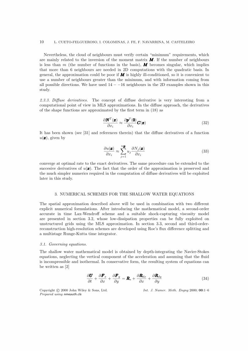
3.1. Governing equations.

The shallow water mathematical model is obtained by depth-integrating the Navier-Stokesequations, neglecting the vertical component of the acceleration and assuming that the fluidis incompressible and isothermal. In conservative form, the resulting system of equations canbe written as [2]

∂UUUUUUUUUUUUUU

∂t+

∂FFFFFFFFFFFFFF x

∂x+

∂FFFFFFFFFFFFFF y

∂y= RRRRRRRRRRRRRRs +

∂RRRRRRRRRRRRRRdx

∂x+

∂RRRRRRRRRRRRRRdy

∂y(34)



being

UUUUUUUUUUUUUU =

hhux

huy

(35)

FFFFFFFFFFFFFF x =

hux

hu2x + 1

2g(h2 −H2)huxuy

FFFFFFFFFFFFFF y =

huy

huxuy

hu2y + 1

2g(h2 −H2)

(36)

RRRRRRRRRRRRRRdx =

02νh∂ux

∂x

νh

(∂uy

∂x+ ∂ux

∂y

)

RRRRRRRRRRRRRRdy =

0

νh

(∂uy

∂x+ ∂ux

∂y

)

2νh∂uy

∂y

(37)

RRRRRRRRRRRRRRS =

0

g(h−H)∂H∂x

− gn2|uuuuuuuuuuuuuu|ux

h1/3

g(h−H)∂H∂y

− gn2|uuuuuuuuuuuuuu|uy

h1/3

(38)

In the above, uuuuuuuuuuuuuu = (ux, uy) is the depth-averaged velocity, h is the total height of fluid, H isa certain reference level (mean water level), g is the gravity acceleration and ν is the eddyviscosity coefficient. The Chezy-Manning formula has been used to model the bottom friction,where n represents the Manning friction coefficient. Coriolis acceleration, surface traction andvariable atmospheric pressure effects have been neglected.

3.2. The one-step Lax-Wendroff scheme.

The Lax-Wendroff time marching algorithm is obtained by performing a second order Taylorseries expansion in time about t = tn, as

UUUUUUUUUUUUUUn+1 = UUUUUUUUUUUUUUn + ∆t

(∂UUUUUUUUUUUUUU

∂t

)n

+∆t2

2

(∂2UUUUUUUUUUUUUU

∂t2

)n

(39)

The time derivatives are expressed in terms of spatial derivatives using the original equation(34), to yield [2]

UUUUUUUUUUUUUUn+1 = UUUUUUUUUUUUUUn + ∆t

(RRRRRRRRRRRRRRs +

∂RRRRRRRRRRRRRRdi

∂xi− ∂FFFFFFFFFFFFFF i

∂xi

)n

+

+∆t2

2

GGGGGGGGGGGGGG

(RRRRRRRRRRRRRRs − ∂FFFFFFFFFFFFFF i

∂xi

)− ∂

∂xi

[AAAAAAAAAAAAAAi

(RRRRRRRRRRRRRRs − ∂FFFFFFFFFFFFFF j

∂xj

)]n

(40)

where all derivatives of order higher than second have been dropped. The notation

∂FFFFFFFFFFFFFF i

∂xi=

∂FFFFFFFFFFFFFF x

∂x+

∂FFFFFFFFFFFFFF y

∂y,

∂RRRRRRRRRRRRRRdi

∂xi=

∂RRRRRRRRRRRRRRdx

∂x+

∂RRRRRRRRRRRRRRdy

∂y(41)

∂

∂xi

[AAAAAAAAAAAAAAi


∂xj

)]=

∂

∂x

[AAAAAAAAAAAAAAx


∂xj

)]+

∂

∂y

[AAAAAAAAAAAAAAy


∂xj

)](42)



has been used for simplicity, and

AAAAAAAAAAAAAAx =∂FFFFFFFFFFFFFF x

∂UUUUUUUUUUUUUU, AAAAAAAAAAAAAAy =

∂FFFFFFFFFFFFFF y

∂UUUUUUUUUUUUUU, GGGGGGGGGGGGGG =

∂RRRRRRRRRRRRRRs

∂UUUUUUUUUUUUUU(43)

are the jacobian matrices of the convective fluxes and source term, respectively. The particularexpression for GGGGGGGGGGGGGG depends on the source terms considered. The jacobians AAAAAAAAAAAAAAx and AAAAAAAAAAAAAAy are

AAAAAAAAAAAAAAx =

0 1 0−u2

x + gh 2ux 0−uxuy uy ux

, AAAAAAAAAAAAAAy =

0 0 1−uxuy uy ux

−u2y + gh 0 2uy

(44)

The integration of (40) over a cell (control volume) Ω yields:

∫

Ω

∆UUUUUUUUUUUUUUdΩ = ∆t

∫

Ω

(RRRRRRRRRRRRRRs +

∂RRRRRRRRRRRRRRdi

∂xi− ∂FFFFFFFFFFFFFF i

∂xi

)n

dΩ+

+∆t2

2

∫

Ω

GGGGGGGGGGGGGG


∂xi

)− ∂

∂xi

[AAAAAAAAAAAAAAi


∂xj

)]n

dΩ (45)

Making use of the divergence theorem, and rearranging,

∫

Ω


∫

Γ

(RRRRRRRRRRRRRRd −FFFFFFFFFFFFFF)n · nnnnnnnnnnnnnn dΓ− ∆t2

2

∫

Γ

SSSSSSSSSSSSSSn · nnnnnnnnnnnnnn dΓ+

+∆t

∫

Ω

RRRRRRRRRRRRRRns dΩ +

∆t2

2

∫

Ω

[GGGGGGGGGGGGGG


∂xi

)]n

dΩ (46)

where nnnnnnnnnnnnnn is the outward pointing unit normal to the boundary Γ and

FFFFFFFFFFFFFF = (FFFFFFFFFFFFFF x, FFFFFFFFFFFFFF y) , RRRRRRRRRRRRRRd = (RRRRRRRRRRRRRRdx,RRRRRRRRRRRRRRdy) , SSSSSSSSSSSSSS =(

AAAAAAAAAAAAAAx


∂xj

),AAAAAAAAAAAAAAy


∂xj

))(47)

In the absence of source terms, RRRRRRRRRRRRRRs = 00000000000000 and equation (46) reduces to

∫

Ω


∫

Γ

(RRRRRRRRRRRRRRd −FFFFFFFFFFFFFF)n · nnnnnnnnnnnnnn dΓ +∆t2

2

∫

Γ

(AAAAAAAAAAAAAAx

∂FFFFFFFFFFFFFF j

∂xjnx + AAAAAAAAAAAAAAy

∂FFFFFFFFFFFFFF j

∂xjny

)n

dΓ (48)

Adopting a standard finite volume discretization for (46), surface integrals are computed usingthe centerpoints of each cell, where the primitive variables are stored, and boundary integralsare evaluated at certain representative points (e.g. at the center of each face). Thus, the discreteequation for each cell I results

∆UUUUUUUUUUUUUU IAI = ∆t

nface∑

iface

(RRRRRRRRRRRRRRd −FFFFFFFFFFFFFF)niface · nnnnnnnnnnnnnnifaceLiface − ∆t2

2

nface∑

iface

SSSSSSSSSSSSSSniface · nnnnnnnnnnnnnnifaceLiface+

+∆tRRRRRRRRRRRRRRnsIAI +

∆t2

2

[GGGGGGGGGGGGGG


∂xj

)]n

I

AI (49)

where AI is the area of cell I, nfaceI the number of cell faces, Liface the longitude of faceiface and UUUUUUUUUUUUUU I the average value of UUUUUUUUUUUUUU over the cell I (associated to the cell center).



3.2.1. Spatial approximation. The final numerical algorithm is obtained after introducing thespatial approximation presented in section 2 into the above general formulation. Recall theMLS approximation φ(xxxxxxxxxxxxxx) of a function φ(xxxxxxxxxxxxxx), given by

φ(xxxxxxxxxxxxxx) =nxxxxxxxxxxxxxx∑

j=1

φjNj(xxxxxxxxxxxxxx) (50)

in terms of the values of the variables φj , j = 1, . . . , nxxxxxxxxxxxxxx at nxxxxxxxxxxxxxx neighbouring cell centers. Theapproximate gradient ∇∇∇∇∇∇∇∇∇∇∇∇∇∇φ is computed as

∇∇∇∇∇∇∇∇∇∇∇∇∇∇φ(xxxxxxxxxxxxxx) =nxxxxxxxxxxxxxx∑

j=1

φj∇∇∇∇∇∇∇∇∇∇∇∇∇∇Nj(xxxxxxxxxxxxxx) (51)

This interpolation scheme provides the basis to reconstruct the necessary information at thecell faces. Assuming a group representation, convective fluxes are first computed at cell centersusing the cell-average information and then interpolated at cell faces as

FFFFFFFFFFFFFF x(xxxxxxxxxxxxxxiface) =ni∑

j=1

FFFFFFFFFFFFFF xjNj(xxxxxxxxxxxxxxiface), FFFFFFFFFFFFFF y(xxxxxxxxxxxxxxiface) =ni∑

j=1

FFFFFFFFFFFFFF yjNj(xxxxxxxxxxxxxxiface) (52)

where, for simplicity, ni = nxxxxxxxxxxxxxxifacedenotes the number of cell-centers taken into account in the

reconstruction process. Similarly, other required entities are interpolated as

RRRRRRRRRRRRRRs(xxxxxxxxxxxxxxiface) =ni∑

j=1

RRRRRRRRRRRRRRsjNj(xxxxxxxxxxxxxxiface),∂FFFFFFFFFFFFFF k

∂xk

∣∣∣∣xxxxxxxxxxxxxxiface

=ni∑

j=1

(FFFFFFFFFFFFFF xj , FFFFFFFFFFFFFF yj) · ∇∇∇∇∇∇∇∇∇∇∇∇∇∇Nj(xxxxxxxxxxxxxxiface) (53)

AAAAAAAAAAAAAAx(xxxxxxxxxxxxxxiface) =ni∑

j=1

AAAAAAAAAAAAAAxjNj(xxxxxxxxxxxxxxiface), AAAAAAAAAAAAAAy(xxxxxxxxxxxxxxiface) =ni∑

j=1

AAAAAAAAAAAAAAyjNj(xxxxxxxxxxxxxxiface), (54)

Diffusive fluxes are not computed following this scheme, but directly at cell faces. For suchpurpose, the velocity gradient is required at the face integration points, which is computed as

∇∇∇∇∇∇∇∇∇∇∇∇∇∇ux(xxxxxxxxxxxxxxiface) =ni∑

j=1

uxj∇∇∇∇∇∇∇∇∇∇∇∇∇∇Nj(xxxxxxxxxxxxxxiface), ∇∇∇∇∇∇∇∇∇∇∇∇∇∇uy(xxxxxxxxxxxxxxiface) =ni∑

j=1

uyj∇∇∇∇∇∇∇∇∇∇∇∇∇∇Nj(xxxxxxxxxxxxxxiface), (55)

or, in compact form,

∇∇∇∇∇∇∇∇∇∇∇∇∇∇uuuuuuuuuuuuuu(xxxxxxxxxxxxxxiface) =ni∑

j=1

uuuuuuuuuuuuuuj ⊗∇∇∇∇∇∇∇∇∇∇∇∇∇∇Nj(xxxxxxxxxxxxxxiface), (56)

In general, any variable and its gradient can be computed using equations (50) and (51) andthe information stored at the cell centers.



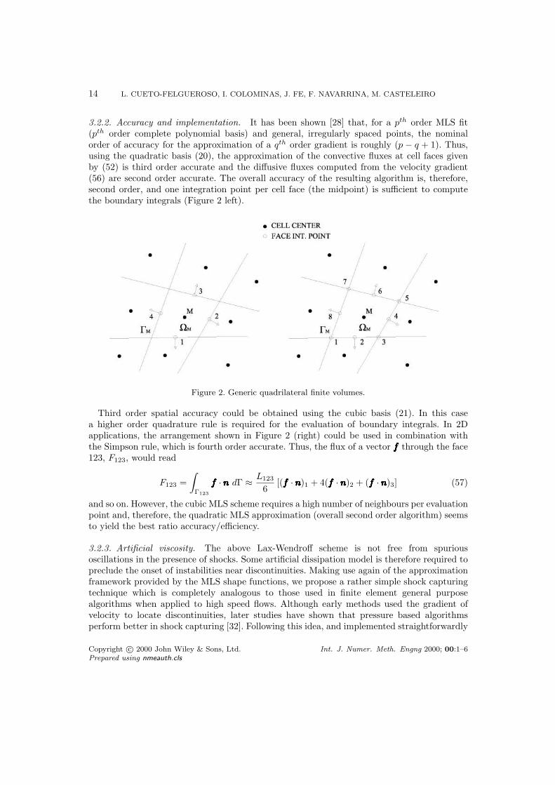
3.2.2. Accuracy and implementation. It has been shown [28] that, for a pth order MLS fit(pth order complete polynomial basis) and general, irregularly spaced points, the nominalorder of accuracy for the approximation of a qth order gradient is roughly (p − q + 1). Thus,using the quadratic basis (20), the approximation of the convective fluxes at cell faces givenby (52) is third order accurate and the diffusive fluxes computed from the velocity gradient(56) are second order accurate. The overall accuracy of the resulting algorithm is, therefore,second order, and one integration point per cell face (the midpoint) is sufficient to computethe boundary integrals (Figure 2 left).

Figure 2. Generic quadrilateral finite volumes.

Third order spatial accuracy could be obtained using the cubic basis (21). In this casea higher order quadrature rule is required for the evaluation of boundary integrals. In 2Dapplications, the arrangement shown in Figure 2 (right) could be used in combination withthe Simpson rule, which is fourth order accurate. Thus, the flux of a vector ffffffffffffff through the face123, F123, would read

F123 =∫

Γ123

ffffffffffffff · nnnnnnnnnnnnnn dΓ ≈ L123

6[(ffffffffffffff · nnnnnnnnnnnnnn)1 + 4(ffffffffffffff · nnnnnnnnnnnnnn)2 + (ffffffffffffff · nnnnnnnnnnnnnn)3] (57)

and so on. However, the cubic MLS scheme requires a high number of neighbours per evaluationpoint and, therefore, the quadratic MLS approximation (overall second order algorithm) seemsto yield the best ratio accuracy/efficiency.

3.2.3. Artificial viscosity. The above Lax-Wendroff scheme is not free from spuriousoscillations in the presence of shocks. Some artificial dissipation model is therefore required topreclude the onset of instabilities near discontinuities. Making use again of the approximationframework provided by the MLS shape functions, we propose a rather simple shock capturingtechnique which is completely analogous to those used in finite element general purposealgorithms when applied to high speed flows. Although early methods used the gradient ofvelocity to locate discontinuities, later studies have shown that pressure based algorithmsperform better in shock capturing [32]. Following this idea, and implemented straightforwardly



as an “added viscosity” rather than a “smoothing” of the variables (as is commonly employedin high speed flow computations), we add the shock capturing viscous fluxes, RRRRRRRRRRRRRRSC

dx and RRRRRRRRRRRRRRSCdy ,

to the right hand side of (34) as

∂UUUUUUUUUUUUUU

∂t+

∂FFFFFFFFFFFFFF x

∂x+

∂FFFFFFFFFFFFFF y


∂(RRRRRRRRRRRRRRdx + RRRRRRRRRRRRRRSCdx )

∂x+

∂(RRRRRRRRRRRRRRdy + RRRRRRRRRRRRRRSCdy )

∂y(58)

where

RRRRRRRRRRRRRRSCdx =

νSCh

∂h∂x

2νSCV h∂ux

∂x

νSCV h

(∂uy

∂x+ ∂ux

∂y

)

RRRRRRRRRRRRRRSC

dy =

νSCh

∂h∂y

νSCV h

(∂uy

∂x+ ∂ux

∂y

)

2νSCV h

∂uy

∂y

(59)

and the shock capturing viscosities

νSCh = Chε2

|uuuuuuuuuuuuuu|+ c

h|∇∇∇∇∇∇∇∇∇∇∇∇∇∇h|, νSC

V = CV ε2|uuuuuuuuuuuuuu|+ c

h|∇∇∇∇∇∇∇∇∇∇∇∇∇∇h| (60)

In these expressions, ε is a characteristic length (e.g. the typical mesh spacing), c is thegravity wave celerity and Ch and CV are parameters that control the amount of artificialdissipation. The required flow information, h, uuuuuuuuuuuuuu and ∇∇∇∇∇∇∇∇∇∇∇∇∇∇h, is computed at cell faces using theMLS approximation. In the case of transcritical flows, an entropy fix scheme should also beincluded in this formulation [33].

3.3. Upwind schemes: high-order reconstruction.

High-resolution schemes based on Riemann solvers are widely recognized as powerfulcomputational tools to handle highly convective flows, including shock wave propagation.Recent studies have shown their superior performance, compared to artificial viscosity schemes[34]. Unfortunately, upwind schemes are frequently associated to an excessive numericaldissipation in more general flows [13], [14], [15], being rather widely regarded as “specialized”methods, and not well suited for more general flows [34].

A quite popular approach to reduce the amount of numerical dissipation of the upwindscheme is the development of a higher-order reconstruction of the field variables inside each cell,requiring the evaluation of gradients and, eventually, higher order derivatives. On unstructuredmeshes, it is difficult to obtain reconstructions of order higher than second using existingprocedures, and even the development of second-order algorithms with low grid sensitivityis not straightforward [30]. It is in this context that the interesting features of meshfreeinterpolation schemes such as MLS, particularly well suited to provide accurate derivativeson irregularly spaced points [28], can be exploited.

This section presents a low-dissipative upwind scheme, based on Roe’s flux differencesplitting, applied to the set of shallow water equations on unstructured meshes. Second andthird-order-reconstruction schemes are developed, using MLS approximation to compute firstand second order derivatives of the flow variables.

Recall the shallow water equations written in conservative form (34)



∂UUUUUUUUUUUUUU

∂t+

∂FFFFFFFFFFFFFF x

∂x+

∂FFFFFFFFFFFFFF y


∂RRRRRRRRRRRRRRdx

∂x+

∂RRRRRRRRRRRRRRdy

∂y(61)

Integrating over a control volume Ω, and using the divergence theorem,∫

Ω

∂UUUUUUUUUUUUUU

∂tdΩ =

∫

Γ

(RRRRRRRRRRRRRRd −FFFFFFFFFFFFFF) · nnnnnnnnnnnnnn dΓ +∫

Ω

RRRRRRRRRRRRRRsdΩ (62)

where nnnnnnnnnnnnnn is the outward pointing unit normal to the boundary Γ and

FFFFFFFFFFFFFF = (FFFFFFFFFFFFFF x, FFFFFFFFFFFFFF y) , RRRRRRRRRRRRRRd = (RRRRRRRRRRRRRRdx,RRRRRRRRRRRRRRdy) (63)

A finite volume discretization leads to a system of ordinary differential equations

∂UUUUUUUUUUUUUU I

∂t=

1AI

nfaceI∑

iface=1

[(RRRRRRRRRRRRRRd −FFFFFFFFFFFFFF) · nnnnnnnnnnnnnn]iface Liface + RRRRRRRRRRRRRRsI (64)

where AI is the area of cell I, nfaceI the number of cell faces, Liface the longitude of faceiface and UUUUUUUUUUUUUU I the average value of UUUUUUUUUUUUUU over the cell I (customarily associated to the cell center).Standard ODE solvers can be applied to (64). We have used Shu’s third order Runge-Kuttaalgorithm, which is compatible with TVD, TVB and ENO schemes [35]

U1 = Un + ∆tL(Un)

U2 =34Un +

14U1 +

14∆tL(U1)

Un+1 =13Un +

23U2 +

23∆tL(U2)

(65)

In the above equations, the operator L(·) represents the right hand side of (64). The diffusivefluxes are evaluated using the same procedure as in the Lax-Wendroff scheme, computingvelocity gradients at cell faces by means of the MLS approximation. The numerical convectivefluxes are obtained using Roe’s flux difference splitting [19] . For this purpose, left (UUUUUUUUUUUUUU−) andright (UUUUUUUUUUUUUU+) states are defined on each face. The numerical flux is then computed as [36]

(FFFFFFFFFFFFFF x, FFFFFFFFFFFFFF y) · nnnnnnnnnnnnnn =12

[(FFFFFFFFFFFFFF x

(UUUUUUUUUUUUUU−)

, FFFFFFFFFFFFFF y

(UUUUUUUUUUUUUU−))

+(FFFFFFFFFFFFFF x

(UUUUUUUUUUUUUU+

), FFFFFFFFFFFFFF y

(UUUUUUUUUUUUUU+

))] · nnnnnnnnnnnnnn− 12|JJJJJJJJJJJJJJ | (UUUUUUUUUUUUUU+ −UUUUUUUUUUUUUU−)

(66)

where JJJJJJJJJJJJJJ(UUUUUUUUUUUUUU+,UUUUUUUUUUUUUU−)

is an approximate flux jacobian, satisfying certain matrix properties [36].Equation (66) can be also written as [37]

(FFFFFFFFFFFFFF x, FFFFFFFFFFFFFF y) · nnnnnnnnnnnnnn =12

[(FFFFFFFFFFFFFF x

(UUUUUUUUUUUUUU−)

, FFFFFFFFFFFFFF y

(UUUUUUUUUUUUUU−))

+(FFFFFFFFFFFFFF x

(UUUUUUUUUUUUUU+

), FFFFFFFFFFFFFF y

(UUUUUUUUUUUUUU+

))] · nnnnnnnnnnnnnn− 12

3∑

k=1

αk|λk|rrrrrrrrrrrrrrk (67)

where λk, k = 1, 3 and rrrrrrrrrrrrrrk, k = 1, 3 are, respectively, the eigenvalues and eigenvectors ofthe approximate jacobian JJJJJJJJJJJJJJ

(UUUUUUUUUUUUUU+,UUUUUUUUUUUUUU−)



λ1 = uxnx + uyny + c, λ2 = uxnx + uyny, λ3 = uxnx + uyny − c (68)

rrrrrrrrrrrrrr1 =

1ux + cnx

uy + cny

, rrrrrrrrrrrrrr2 =

0−cny

cnx

, rrrrrrrrrrrrrr2 =

1ux − cnx

uy − cny

(69)

and the corresponding wave strengths αk, k = 1, 3

α1 =∆h

2+

12c

(∆ (hux)nx + ∆ (huy)ny − (uxnx + uyny)∆h)

α2 =1c

((∆ (huy)− uy∆(h)) nx − (∆ (hux)− ux∆(h)) ny)

α3 =∆h

2− 1

2c(∆ (hux)nx + ∆ (huy)ny − (uxnx + uyny)∆h)

(70)

where ∆ (·) = (·)+ − (·)−, nnnnnnnnnnnnnn = (nx, ny) is the outward pointing unit normal to the interface,and the Roe-averaged values (computed using UUUUUUUUUUUUUU+ and UUUUUUUUUUUUUU−) are defined as

ux =u+

x

√h+ + u−x

√h−√

h+ +√

h−, uy =

u+y

√h+ + u−y

√h−√

h+ +√

h−, c =

√g (h+ + h−) /2 (71)

A first order scheme is obtained by setting UUUUUUUUUUUUUU− and UUUUUUUUUUUUUU+ to be the variables at the left and rightcell centers. Although first order schemes often provide valuable information for the engineeringpractice, their accuracy is severely undermined by an excess of numerical dissipation. Moreaccurate methods (the so-called higher order schemes) can be devised by choosing “better”values for the left and right states.

3.3.1. Higher order schemes: reconstruction and limiting. As mentioned before, the amountof artificial dissipation can be reduced by expanding the piecewise constant representationwhich the finite volume philosophy entails. This can be addressed by (astutely) choosing“closer” values for UUUUUUUUUUUUUU− and UUUUUUUUUUUUUU+, and several extrapolation procedures are feasible. In thisstudy, a multidimensional reconstruction of the field variables inside each cell is obtained bymeans of Taylor series expansions. Unfortunately, these higher-order extensions of the basiclinear algorithm are not free from oscillations and some kind of limiting procedure is requiredin the presence of shocks.

Second order accuracy is achieved by means of a linear reconstruction inside left and rightcells, as

UUUUUUUUUUUUUU−(xxxxxxxxxxxxxx) = UUUUUUUUUUUUUUM− +∇∇∇∇∇∇∇∇∇∇∇∇∇∇UUUUUUUUUUUUUUM−(xxxxxxxxxxxxxx− xxxxxxxxxxxxxxM−) (72)

UUUUUUUUUUUUUU+(xxxxxxxxxxxxxx) = UUUUUUUUUUUUUUM+ +∇∇∇∇∇∇∇∇∇∇∇∇∇∇UUUUUUUUUUUUUUM+(xxxxxxxxxxxxxx− xxxxxxxxxxxxxxM+) (73)

where UUUUUUUUUUUUUUM− and UUUUUUUUUUUUUUM+ stand for left and right cell-averaged (center) values of the variables, xxxxxxxxxxxxxxM−

and xxxxxxxxxxxxxxM+ are the spatial coordinates of left and right cell centerpoints and ∇∇∇∇∇∇∇∇∇∇∇∇∇∇UUUUUUUUUUUUUUM− and ∇∇∇∇∇∇∇∇∇∇∇∇∇∇UUUUUUUUUUUUUUM+

are cell-centered gradients. These gradients ∇∇∇∇∇∇∇∇∇∇∇∇∇∇UUUUUUUUUUUUUUM− and ∇∇∇∇∇∇∇∇∇∇∇∇∇∇UUUUUUUUUUUUUUM+ are assumed to be constant



on each cell and, therefore, the reconstructed variables are discontinuous across interfaces (i.e.we still have a Riemann problem on each face).

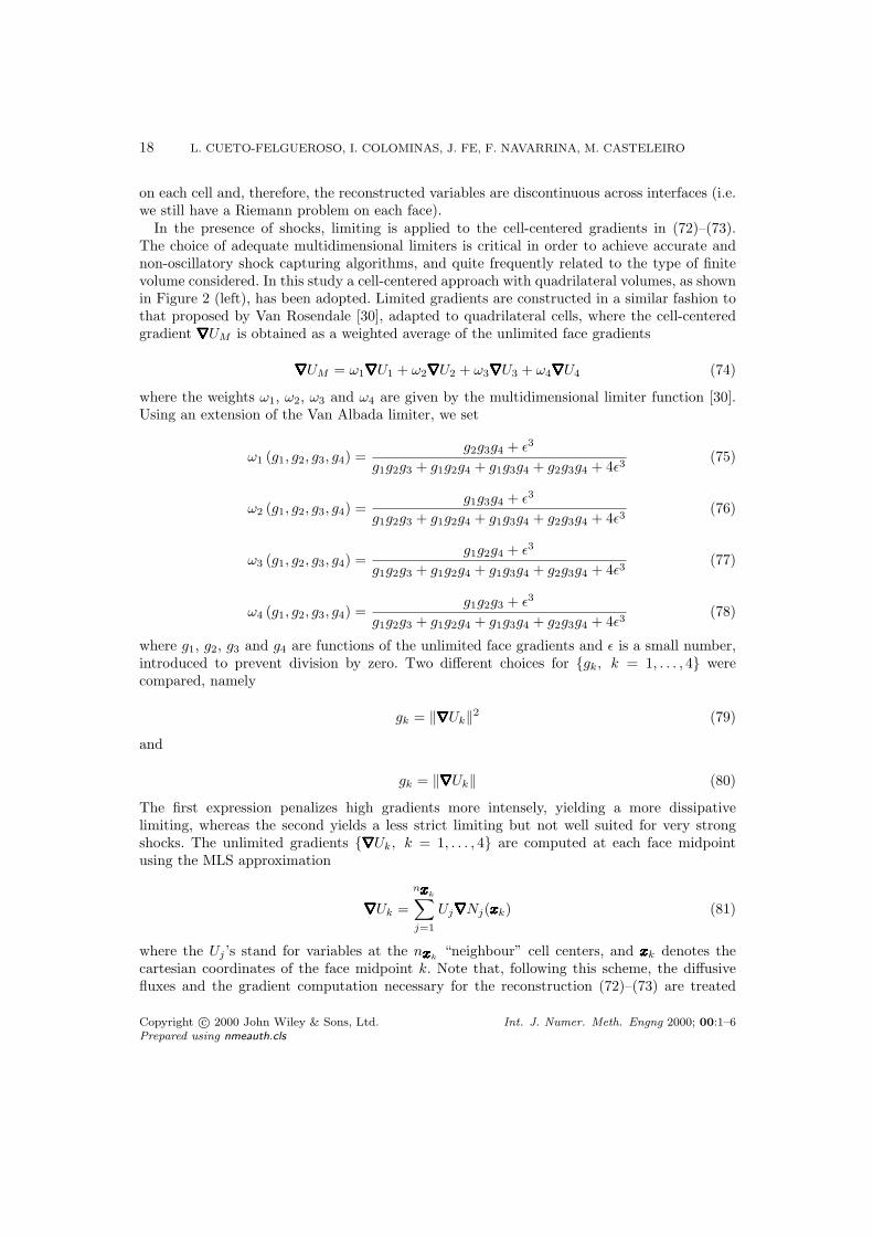
In the presence of shocks, limiting is applied to the cell-centered gradients in (72)–(73).The choice of adequate multidimensional limiters is critical in order to achieve accurate andnon-oscillatory shock capturing algorithms, and quite frequently related to the type of finitevolume considered. In this study a cell-centered approach with quadrilateral volumes, as shownin Figure 2 (left), has been adopted. Limited gradients are constructed in a similar fashion tothat proposed by Van Rosendale [30], adapted to quadrilateral cells, where the cell-centeredgradient ∇∇∇∇∇∇∇∇∇∇∇∇∇∇UM is obtained as a weighted average of the unlimited face gradients

∇∇∇∇∇∇∇∇∇∇∇∇∇∇UM = ω1∇∇∇∇∇∇∇∇∇∇∇∇∇∇U1 + ω2∇∇∇∇∇∇∇∇∇∇∇∇∇∇U2 + ω3∇∇∇∇∇∇∇∇∇∇∇∇∇∇U3 + ω4∇∇∇∇∇∇∇∇∇∇∇∇∇∇U4 (74)

where the weights ω1, ω2, ω3 and ω4 are given by the multidimensional limiter function [30].Using an extension of the Van Albada limiter, we set

ω1 (g1, g2, g3, g4) =g2g3g4 + ε3

g1g2g3 + g1g2g4 + g1g3g4 + g2g3g4 + 4ε3(75)

ω2 (g1, g2, g3, g4) =g1g3g4 + ε3

g1g2g3 + g1g2g4 + g1g3g4 + g2g3g4 + 4ε3(76)

ω3 (g1, g2, g3, g4) =g1g2g4 + ε3

g1g2g3 + g1g2g4 + g1g3g4 + g2g3g4 + 4ε3(77)

ω4 (g1, g2, g3, g4) =g1g2g3 + ε3

g1g2g3 + g1g2g4 + g1g3g4 + g2g3g4 + 4ε3(78)

where g1, g2, g3 and g4 are functions of the unlimited face gradients and ε is a small number,introduced to prevent division by zero. Two different choices for gk, k = 1, . . . , 4 werecompared, namely

gk = ‖∇∇∇∇∇∇∇∇∇∇∇∇∇∇Uk‖2 (79)

and

gk = ‖∇∇∇∇∇∇∇∇∇∇∇∇∇∇Uk‖ (80)

The first expression penalizes high gradients more intensely, yielding a more dissipativelimiting, whereas the second yields a less strict limiting but not well suited for very strongshocks. The unlimited gradients ∇∇∇∇∇∇∇∇∇∇∇∇∇∇Uk, k = 1, . . . , 4 are computed at each face midpointusing the MLS approximation

∇∇∇∇∇∇∇∇∇∇∇∇∇∇Uk =

nxxxxxxxxxxxxxxk∑

j=1

Uj∇∇∇∇∇∇∇∇∇∇∇∇∇∇Nj(xxxxxxxxxxxxxxk) (81)

where the Uj ’s stand for variables at the nxxxxxxxxxxxxxxk“neighbour” cell centers, and xxxxxxxxxxxxxxk denotes the

cartesian coordinates of the face midpoint k. Note that, following this scheme, the diffusivefluxes and the gradient computation necessary for the reconstruction (72)–(73) are treated



within a unified approach (i.e. only the derivatives of the MLS shape functions at the facemidpoints are needed).

The numerical dissipation can be further reduced by considering higher-order Taylor seriesexpansions. A third order reconstruction is developed using cell-centered second derivatives toperform a quadratic expansion of the field variables inside each cell, as

U(xxxxxxxxxxxxxx) = UM +∇∇∇∇∇∇∇∇∇∇∇∇∇∇UM (xxxxxxxxxxxxxx− xxxxxxxxxxxxxxM ) +12(xxxxxxxxxxxxxx− xxxxxxxxxxxxxxM )THHHHHHHHHHHHHHM (xxxxxxxxxxxxxx− xxxxxxxxxxxxxxM )−

12

[Ixx

∂2U

∂x2+ 2Ixy

∂2U

∂x∂y+ Iyy

∂2U

∂y2

](82)

where HHHHHHHHHHHHHHM is the cell-centered hessian matrix and

Ixx =∫

Ω

(x− xM )2dΩ, Ixy =∫

Ω

(x− xM )(y − yM )dΩ, Iyy =∫

Ω

(y − yM )2dΩ (83)

The above integrals can be easily computed for quadrilateral and triangular cells. The lastterm in (82) has been added to ensure that the average value of the reconstructed variablesover cell Ωi is the center value UMi , i.e.

1Ai

∫

xxxxxxxxxxxxxx∈Ωi

U (xxxxxxxxxxxxxx) dΩ = UMi (84)

Note that the introduction of the terms (83) does not reduce the order of the approximationgiven by (82). For the second order derivatives we have used the same limiting procedurepresented above for the first order gradients, (74)–(78). The development of better limiters forthis third-order reconstruction is currently in progress.

3.3.2. Dissipation additions. Some additional dissipation can be necessary in certainapplications. This procedure is frequent in the context of flux difference splitting schemes forgas dynamics in order to break expansion shocks and as a cure for the “carbuncle” phenomenonin supersonic flow past blunt bodies. Yee proposed a formula for Roe’s Riemann solver wherethe eigenvalues λk are replaced by Q(λk, δk), as [38]

Qk(λk, δk) =

λk |λk| < δk

12

[sign(λk)λ2

k+δ2k

δk+ λk

]|λk| ≥ δk

(85)

where

δk = δ∗k (|vn|+ c) (86)

being vn the velocity normal to the grid face and c the face wave speed. The parameters δ∗kcontrol the amount of artificial dissipation. This formula has been found excessively dissipativefor the vn waves [38], and thus not suitable for viscous flow. Inspired by the work of Peery andImlay, Lin [38] proposed a modification for structured meshes which uses the second differenceof the pressure to tune the dissipation. For the vn + c and vn − c waves,

δk = (|vn|+ c) (k1 + k2kp) (87)



instead of (86), whereas for the linear waves

δk = (|vn|+ c) (k3kp) (88)

The coefficient kp is defined at each cell (i, j) as

(kp)i,j =12

(∣∣∣∣Pi+1,j − 2Pi,j + Pi−1,j

Pi+1,j + 2Pi,j + Pi−1,j

∣∣∣∣ +∣∣∣∣Pi,j+1 − 2Pi,j + Pi,j−1

Pi,j+1 + 2Pi,j + Pi,j−1

∣∣∣∣)

(89)

where P denotes pressure. We propose a different expression for kp, as

kp = ε|∇∇∇∇∇∇∇∇∇∇∇∇∇∇P |

P(90)

where ε is a certain characteristic length. For shallow water problems, we write

kp = ε|∇∇∇∇∇∇∇∇∇∇∇∇∇∇h|

h(91)

This parameter is defined in a continuous fashion (in practice it is only required at eachinterface) and computed using the MLS shape functions, which makes this procedure suitablefor unstructured meshes. In this study we define the characteristic length ε as

ε =12

(√A+ +

√A−

)(92)

being A+ and A− the area of the cells on each side of the interface.

3.3.3. Computational aspects: diffuse derivatives. The evaluation of full second orderderivatives of the MLS shape functions is a tedious and computationally expensive task.Instead, we have used the concept of diffuse derivative to approximate the second orderderivatives required in the third order reconstruction (82). Thus, we write

∂2U(xxxxxxxxxxxxxx)∂xαxβ

≈nxxxxxxxxxxxxxx∑

j=1

Uj∂2Nj(xxxxxxxxxxxxxx)∂xαxβ

(93)

where the second derivatives of the shape functions are approximated by

∂2NNNNNNNNNNNNNNT (xxxxxxxxxxxxxx)∂xαxβ

≈ ∂2ppppppppppppppT (00000000000000)∂xαxβ

CCCCCCCCCCCCCC(xxxxxxxxxxxxxx) (94)

and straightforwardly computed once the matrix CCCCCCCCCCCCCC(xxxxxxxxxxxxxx), given by (17) and required to computethe MLS shape functions, is known. Our numerical experiments show that, using the third orderreconstruction (82), the results obtained with diffuse second derivatives are almost identicalto those obtained with full derivatives. This seems to be due to the fact that the order ofaccuracy of the full derivatives is preserved in the diffuse approach.

Full MLS first derivatives have been used in the examples shown below, in order to retain thewhole accuracy of the MLS approximation (not only the order of convergence) in the evaluationof the viscous fluxes. Nevertheless, in the case of inviscid flows, the numerical experiments showagain that diffuse first derivatives could be used for reconstruction purposes with no noticeableloss of accuracy.



4. NUMERICAL EXAMPLES

This section intends to provide further insight into the behaviour of the proposed methodologiesand presents additional information on computational and practical implementation issues.

It is known that high-resolution schemes are particularly well suited to yield accuratesolutions of inviscid flows with shock waves. The ability to accurately capture such complexflows is also tested in the case of the Lax-Wendroff algorithm, combined with a shock-capturingviscosity model.

The dissipation properties of the proposed schemes are also analyzed in the case of viscousflow at moderate and high Reynolds numbers. In the case of smooth viscous flow, the Lax-Wendroff scheme is expected to yield quite accurate solutions, thus representing a goodoportunity to assess the quality of the results provided by the high order upwind schemes.

Special attention is paid to the proposed third-order-reconstruction Roe scheme, in bothinviscid and viscous flow applications. In the latter case, the low-dissipation properties of thisalgorithm look particularly interesting, with substantial improvements with respect to thesecond-order scheme. The unstructered quadrilateral meshes were generated using the codeGEN4U, based on the formulation proposed by Sarrate [39].

4.1. Inviscid flows.

4.1.1. 2D dam break problem. This first example is a rather classical benchmark test fordiscontinuous transient flow solvers. The problem set up is depicted in Figure 3 and correspondsto two reservoirs, with water levels h1 = 10 m and h2 = 5 m respectively, separated by anasymetrically located lockgate, which is “instantaneously” removed at the beginning of thesimulation. Viscosity and bottom friction effects are not considered. The solution at t = 7.2 s(90 time steps) was obtained using the Lax-Wendroff and Roe schemes.

In both cases the MLS shape functions were computed using the quadratic basis (20),with circular supports of radius 2ρ, being ρ = 1.2d and d the typical grid size; in this cased = ∆x = ∆y = 2.5 m.

Second and third-order reconstructions, as exposed in section 3, were developed in orderto obtain higher-order schemes. Slope limiting was carried out using (74)–(78) with either(79) or (80). First order derivatives are full derivatives (given by (18)), whereas second orderderivatives were approximated by the diffuse ones (dropping the succesive derivatives of CCCCCCCCCCCCCC(xxxxxxxxxxxxxx)).

The results for the second order scheme with limited gradients are shown in Figure 4. Thesharp features of the flow are well captured by this scheme without oscillations and it seemsthat the use of (79) yields a slightly less dissipative limiting procedure.

The third-order-reconstruction scheme with limited first and second-order derivatives doesnot appear to produce a significant improvement of the results (Figure 5). We suspect that thisfact is related to the rather strong limiting applied to the second derivatives. The sensitivity ofthe fine scales of the flow to the limiting of high order derivatives is well known in the contextof ENO and WENO schemes [40]. Further insight is provided by the solutions obtained withunlimited derivatives. This problem involves a rather mild shock and can be solved (at leastusing MLS approximation to compute the derivatives) without the introduction of limiters. Inthis case, first and second-order derivatives are computed directly at cell centers. The watersurface contours for the second and third-order schemes are plotted in Figure 6. The second-order scheme without limiters yields a good solution, accurately capturing the shock front.



The third-order scheme produces a less smooth solution, but the front is even sharper thanthat of the second-order scheme.

The Lax-Wendroff scheme must be combined with a shock capturing viscosity model. Themethodology proposed in section 3 includes two free constants, Ch and CV , and requiresthe definition of a characteristic length. The shape (and quality) of the solution is largelyinfluenced by the adequate choice of such parameters. Figure 7 depicts the contours obtainedwith Ch = 0.3 and CV = 0.7 (left), and Ch = 1 and CV = 3 (right). In the first case, theadvancing front is reasonably well captured, but at the cost of slightly less smooth contours.On the other hand, Ch = 1 and CV = 3 yield a smoother but also excessively dissipativesolution. This example illustrates an important drawback of this kind of artificial viscositybased schemes, where an adequate tuning of the shock-capturing model is fundamental toobtain accurate and stable algorithms for each mesh and problem.

The water surface obtained with the second order Roe scheme is plotted in Figure 8.

0 20 40 60 80 100 120 140 160 180 2000

20

40

60

80

100

120

140

160

180

200

75 m

10 m

Lockgate position

95 m

Figure 3. 2D break dam problem set up.

4.1.2. Supercritical flow in a channel with variable width. Given its multiscale nature, theMLS approximation possesses nice properties to be used in adaptive and multigrid strategiesas a means to exchange information between coarse and refined meshes. To illustrate thispoint, let us consider an example of supercritical flow in a symmetrical channel. The initialwidth of 40 m is constricted from both sides with an angle of 15. After the constriction therefollows a straight channel, being the total length of the domain 120 m. The imposed inletflow parameters are: Froude number, Fr = 3, and unit depth, h = 1 m. The steady-state flowwas obtained using the second order Roe scheme. The resuts obtained with the third orderreconstruction were almost identical and are not shown. It was not possible to obtain solutionsof comparable quality using the Lax-Wendroff scheme.

A first rough solution is computed using a coarse mesh (Figure 9, 917 cells). This solution isthe interpolated using the MLS approximation on fine grids, and the computation is continued



Figure 4. 2D break dam problem: surface contours at t = 7.2 s, second order Roe scheme. Limitedgradients using (79) (left) and (80) (right).

Figure 5. 2D break dam problem: surface contours at t = 7.2 s, third order Roe scheme. Limitedderivatives using (79) (left) and (80) (right).

until convergence. Two different grids were used: a uniformly refined mesh with 23349 cells(Figure 11), and an adapted mesh 9216 cells (Figures 10 and 12). Figure 13 depicts a 3D viewof the water surface. The classical cross-wave structure of the flow can be easily identified andthe hydraulic jumps are quite well captured..

4.1.3. Supercritical flow past a cylinder. In this last inviscid case we consider supercriticalflow past a circular cylinder. The flow parameters at the inflow are: Froude number, Fr = 4 andunit water depth, h = 1 m. The flow is impulsively started and some dissipation was neededto avoid instabilities in the early stages of the simulation. Thus, the procedure presented insection 3.3.2 was used at the beginning of the simulation, setting k2 = 2 and k3 = 1 and no base



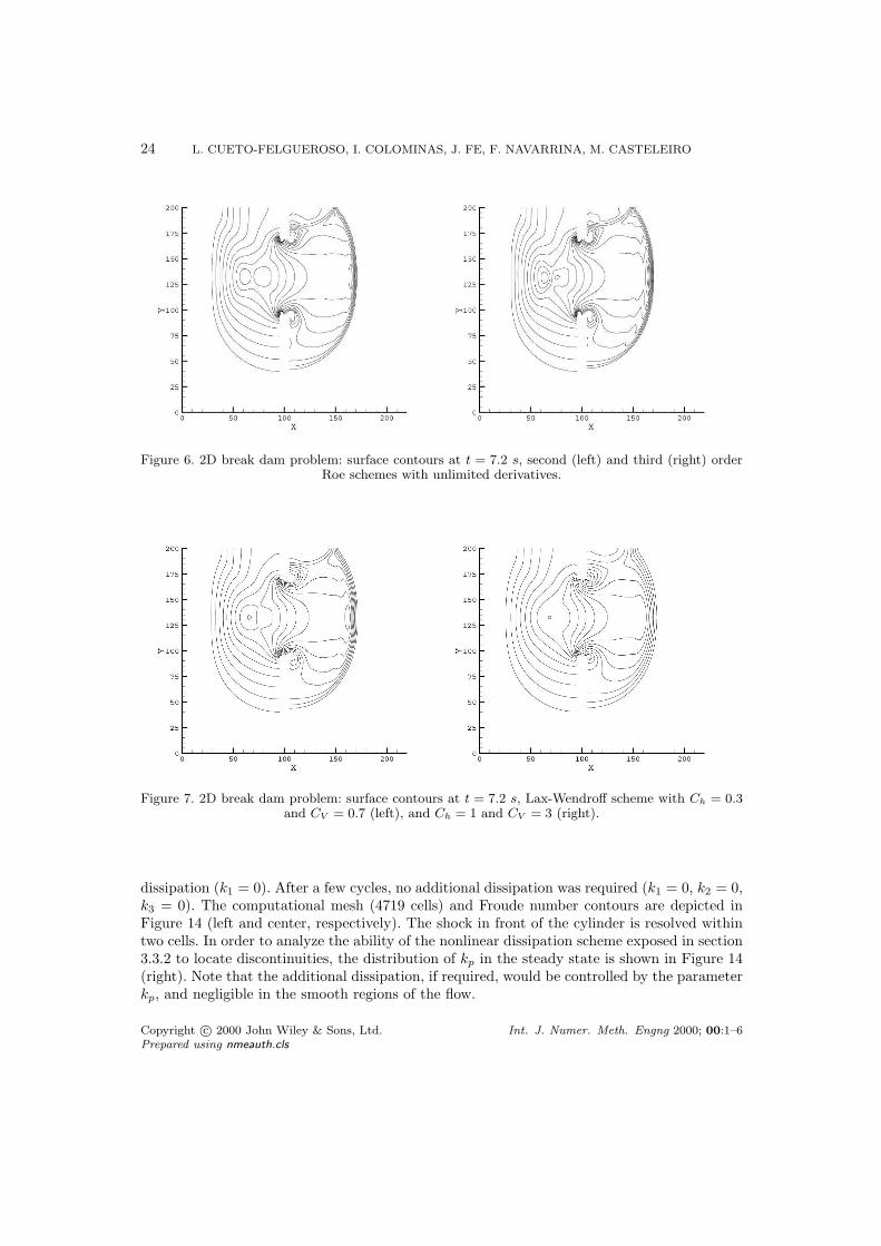
Figure 6. 2D break dam problem: surface contours at t = 7.2 s, second (left) and third (right) orderRoe schemes with unlimited derivatives.

Figure 7. 2D break dam problem: surface contours at t = 7.2 s, Lax-Wendroff scheme with Ch = 0.3and CV = 0.7 (left), and Ch = 1 and CV = 3 (right).

dissipation (k1 = 0). After a few cycles, no additional dissipation was required (k1 = 0, k2 = 0,k3 = 0). The computational mesh (4719 cells) and Froude number contours are depicted inFigure 14 (left and center, respectively). The shock in front of the cylinder is resolved withintwo cells. In order to analyze the ability of the nonlinear dissipation scheme exposed in section3.3.2 to locate discontinuities, the distribution of kp in the steady state is shown in Figure 14(right). Note that the additional dissipation, if required, would be controlled by the parameterkp, and negligible in the smooth regions of the flow.



Figure 8. 2D break dam problem: water surface at t = 7.2 s (second order Roe scheme).

Figure 9. Supercritical channel flow: coarse mesh (917 cells).

4.2. Viscous flows.

We are also interested in flows where viscous and turbulence effects are of the utmostimportance. A suitable numerical method to solve such problems on unstructured meshesshould therefore not introduce excessive numerical dissipation, in order to capture fine viscousfeatures of the flow and to avoid interactions with the turbulence model.

It is crucial to assess whether high-resolution schemes such as Roe’s and its high orderextensions are suitable for general viscous flows. For this purpose, two different test cases areanalyzed in this section, comparing the results with those of the low dissipative Lax-Wendroffscheme.

The first example intends to evaluate the influence of the limiting procedure on the accuracy



Figure 10. Supercritical channel flow: adapted mesh (9216 cells).

Figure 11. Supercritical channel flow: water surface contours (fine mesh).

Figure 12. Supercritical channel flow: water surface contours (adapted mesh).



Figure 13. Supercritical channel flow: 3D view of the computed water surface.

of viscous computations, whereas the second one involves a smooth flow where limiters are notneeded, thus providing a closer insight into the intrinsic numerical dissipation of the differentschemes.

4.2.1. Supercritical viscous flow near a wall. In analogy with a classical benchmark testfor compressible flow solvers, we consider viscous supercritical flow near a solid wall. Theproblem statement is exposed in Figure 15. The free stream flow parameters are: Froudenumber, Fr = 1.5, unit depth, h = 1 m and Reynolds number Re = 1000, referred to a unitreference length, L = 1 m. No-slip boundary conditions were applied along the wall boundary,y = 0, 0.2 ≤ x ≤ 0.8. The flow pattern includes a shock front starting from the leading edge ofthe wall and a boundary layer (assumed here to be laminar) due to the presence of the no-slipcondition.

The problem was run on two different meshes, plotted in Figures 16 and 17. The first is astructured non-uniform mesh, whereas the second is a (roughly) adapted, fully unstructeredmesh. In the first case, and given the mesh structure, the MLS shape functions were computedusing anisotropic weighting, according to (26).

Figures 18 and 19 show the computed Froude number profiles along the outlet section,with respectively limited and unlimited derivatives to develop the second and third orderreconstructions in the Roe schemes. For the Lax-Wendroff scheme the artificial viscosity modelexposed in section 3.2.3 was used, with Ch = Cv = 0.1. The unlimited Roe schemes look lessdissipative than the Lax-Wendroff scheme with artificial viscosity. The solution provided bythe third order scheme is slightly better than that of the second order scheme even at thismoderate Reynolds number.



Figure 14. Supercritical flow past a cylinder (Fr = 4): computational mesh (4719 cells, left), Froudenumber contours (center) and distribution of kp (right)

Even though the limiting procedure adds more dissipation in the smooth regions of the flow,the results and reasonably close to those of the unlimited reconstructions. The Froude numbercontours for the third order Roe scheme are plotted in Figures 16 (right) and 17 (right).

4.2.2. Lid driven cavity flow Although this is not a standard test in the shallow waterliterature (and is probably devoid of any hydraulic meaning), we have found this problem veryuseful to assess the ability of the different numerical schemes to capture fine viscous features ofthe flow. The problem set up is completely analogous to the classical cavity flow problem usedto validate incompressible Navier-Stokes solvers. A unit square domain with flat, frictionlessbotton is considered. The boundary conditions imposed are h = 1 m, qx = 1 m2/s and qy = 0on y = 1 m (including the corners) and solid walls (qx = 0 and qy = 0) elsewhere. Unit waterdepths were also imposed on the inferior corners. The computational mesh employed is shownin Figure 20, and consists in 61x61 non-uniform cells. The grid has been refined near solidwalls to account for the thin boundary layer.

The problem was solved for Reynolds numbers of 1000 and 10000. For comparison purposes,the solutions were also obtained on the same mesh using the finite element Taylor-Galerkinexplicit formulation developed by Peraire [1],[2].

Given the absence of shocks, the Lax-Wendroff scheme was used without the introduction of



Figure 15. Supercritical viscous flow near a wall: problem set up.

Figure 16. Supercritical viscous flow near a wall: structured computational mesh (4875 cells) andFroude number contours (right). Third order Roe scheme.



Figure 17. Supercritical viscous flow near a wall: unstructured computational mesh (5426 cells) andFroude number contours (right). Third order Roe scheme.

Figure 18. Supercritical viscous flow near a wall: Froude number profiles along x = 0.8 m (left) andclose up comparison (right). Limited reconstructions.

any artificial dissipation model, and it was not necessary to use limiters in the reconstructionprocess for the Roe schemes. Instead of using the limiting formula (74), the correspondinglinear and quadratic reconstructions (given by (72)–(73) and (82) respectively) were performedwith first and second-order derivatives computed directly at cell centers using the MLS shape



Figure 19. Supercritical viscous flow near a wall: Froude number profiles along x = 0.8 m (left) andclose up comparison (right). Unlimited reconstructions.

functions. All first derivatives (the face derivatives used for the viscous fluxes and the cell-center derivatives used for the reconstruction) are full MLS derivatives, whereas the second-order derivatives used in the quadratic reconstruction are diffuse ones. Given the presence ofhighly stretched cells near the walls, anisotropic weighting was used according to (26).

The streamlines for the Lax-Wendroff and third-order Roe scheme are depicted in Figures21–22. The horizontal velocity (ux) profiles along x = 0.5 m for the Taylor-Galerkin, Lax-Wendroff and Roe schemes are plotted in Figures 23–24.

The different schemes yield almost identical solutions at moderate Reynolds numbers(Re = 1000, Fig. 23). However, at high Reynolds numbers (Re = 10000, Fig. 24) the dissipationproperties of each scheme become more evident. The results obtained with the FEM Taylor-Galerkin and the proposed FV Lax-Wendroff schemes are very similar, although the latterpredicts slightly higher maximum horizontal velocities, which could be considered a moreaccurate solution.

The second and third-order-reconstruction Roe schemes provide acceptable solutions forRe = 10000. However, the maximum horizontal velocities are somewhat displaced from theircorrect position closer to the wall, affecting the shape of the profile. This effect could beassociated to an excess of crosswind dissipation introduced by the upwind scheme. It isremarkable that this excessive dissipation is substantially reduced by the proposed third-order reconstruction (Figure 24). The solution obtained with this latter approach is in betteragreement with that of the more general Taylor-Galerkin and Lax-Wendroff schemes.

5. CONCLUSIONS

In this paper we explored the ability of a meshfree interpolation technique (namely, theMoving Least-Squares method) to be used in combination with finite volume discretizations on



0 0.1 0.2 0.3 0.4 0.5 0.6 0.7 0.8 0.9 10

0.1

0.2

0.3

0.4

0.5

0.6

0.7

0.8

0.9

1

Figure 20. Lid driven cavity flow: computational mesh.

Figure 21. Lid driven cavity flow: streamlines for Re = 1000. Lax-Wendroff (left) and third order Roe(right) schemes.

unstructured grids. The resulting numerical schemes were applied to the resolution of the set ofshallow water equations. We were particularly interested in the development of low-dissipativehigh order upwind schemes, given their robustness and shock-capturing ability. In addition,and making use of the general approximation framework provided by the MLS approach, asecond-order accurate in time Lax-Wendroff scheme was developed, with accuracy and stabilityproperties very similar to those of its FEM counterpart, the Taylor-Galerkin method. A shock-capturing artificial viscosity model was proposed for this Lax-Wendroff scheme.

The development of high order upwind schemes on unstructured grids involves high-order



Figure 22. Lid driven cavity flow: streamlines for Re = 10000. Lax-Wendroff (left) and third orderRoe (right) schemes.

−0.5 −0.25 0 0.25 0.5 0.75 10

0.1

0.2

0.3

0.4

0.5

0.6

0.7

0.8

0.9

1FEM Taylor−GalerkinFV Lax−Wendroff (MLS)FV Roe (third order)FV Roe (second order)

Figure 23. Lid driven cavity flow: profiles of ux along x = 0.5 for Re = 1000.

reconstruction of the field variables or fluxes inside each cell. The main difficulty at this point isassociated to the accurate evaluation of gradients and, eventually, higher-order derivatives. Itwas shown in this study that the class of approximation methods employed in the “meshfree”literature (of which the MLS technique is one example) is particularly well suited for suchpurpose, allowing, in addition, an accurate computation of the viscous fluxes. They provide



−0.5 −0.25 0 0.25 0.5 0.75 10

0.1

0.2

0.3

0.4

0.5

0.6

0.7

0.8

0.9

1FEM Taylor−GalerkinFV Lax−Wendroff (MLS)FV Roe (third order)FV Roe (second order)

Figure 24. Lid driven cavity flow: profiles of ux along x = 0.5 for Re = 10000.

a robust and general approximation framework which contitutes an interesting alternative tothe more or less “heuristic” existing techniques.

As expected, the performance of the more “specialized” Roe schemes in complex flowsinvolving shock waves is superior to that of the Lax-Wendroff scheme with the proposedartificial viscosity model. On the other hand, the upwind schemes yield more dissipativesolutions in the cavity flow test. However, the third-order-reconstruction Roe scheme developedhere shows substantial improvements with respect to the second-order scheme, in goodagreement with the results obtained with the more general Taylor-Galerkin and Lax-Wendroffalgorithms. A more complete assessment of the suitability of this scheme for turbulent flowcomputations is currently in progress. The results obtained in this study for viscous flow athigh Reynolds numbers are encouraging.

ACKNOWLEDGEMENTS

This work has been partially supported by the SGPICT of the “Ministerio de Ciencia yTecnologıa” of the Spanish Government (Grant DPI# 2001-0556), the “Xunta de Galicia” (Grants #PGDIT01PXI11802PR and PGIDIT03PXIC118002PN) and the University of La Coruna.

Mr. Cueto-Felgueroso gratefully acknowledges the support received from “Fundacion de la IngenierıaCivil de Galicia” and “Colegio de Ingenieros de Caminos, Canales y Puertos”. Most of this paper waswritten while Mr. Cueto-Felgueroso was visiting the University of Wales Swansea during the firstsemester of 2004. The support received from “Caixanova” and the kind hospitality offered by Prof.Javier Bonet and his research group are gratefully acknowledged.

REFERENCES



1. J. Peraire. A finite element method for convection dominated flows. PhD Thesis. University of WalesSwansea (1986).

2. J. Peraire, O.C. Zienkiewicz, K. Morgan. Shallow water problems: a general explicit formulation.International Journal for Numerical Methods in Engineering. 22:547–574 (1986).

3. M. Quecedo, M. Pastor. A reappraisal of Taylor-Galerkin algorithm for drying-wetting areas in shallowwater computations. International Journal for Numerical Methods in Fluids. 38:515–531 (2002).

4. M. Quecedo, M. Pastor. Finite element modelling of free surface flows on inclined and curved beds. Journalof Computational Physics. 189:45–62 (2003).

5. T.W.H. Sheu, C.C. Fang. High resolution finite-element analysis of shallow water equations in twodimensions. Computer Methods in Applied Mechanics and Engineering. 190:2581–2601 (2001).

6. F. Alcrudo, P. Garcıa-Navarro. A high-resolution Godunov-type scheme in finite volumes for the 2D shallow-water equations. International Journal for Numerical Methods in Fluids. 16:489–505 (1993).

7. D.H. Zhao, H.W. Shen, G.Q. Tabious III, J.S. Lai, W.Y. Tan. Finite-volume two-dimensional unsteady-flowmodel for river basins. ASCE Journal of Hydraulic Engineering. 120:864–883 (1994).

8. K. Anastasiou, C.T. Chan. Solution of the 2D shallow water equations using the finite volume methodon unstructured triangular meshes. International Journal for Numerical Methods in Fluids. 24:1225–1245(1997).

9. K. Hu, C.G. Mingham, D.M. Causon. A bore-capturing finite volume method for open-channel flows.International Journal for Numerical Methods in Fluids. 28:1241–1261 (1998).

10. M.H. Tseng. Explicit finite volume non-oscillatory schemes for 2D transient free-surface flows. InternationalJournal for Numerical Methods in Fluids. 30:831–843 (1999).

11. R. Liszka, B. Wendroff. Two-dimensional shallow water equations by composite schemes. InternationalJournal for Numerical Methods in Fluids. 30:461–479 (1999).

12. J. Wang, R. Liu. The composite finite volume method on unstructured meshes for the two-dimensionalshallow water equations. International Journal for Numerical Methods in Fluids. 37:933–949 (2001).

13. J. Fe. A finite volume numerical formulation for shallow water turbulent flows. PhD Thesis. Universidadde A Coruna (2004).

14. T. Bui. A parallel, finite-volume algorithm for large-eddy simmulation of turbulent flows. Computers andFluids. 29:877–915 (2000).

15. S.Y. Lin, Y.F. Chen, S.C. Shih. Numerical study of MUSCL schemes for computational aeroacoustics.AIAA–97–0023. (1997).

16. V. Daru, C. Tenaud. High order one-step monotonicity-preserving schemes for unsteady compressible flowcalculations. Journal of Computational Physics. 193:563–594 (2004).

17. P. Lancaster, K. Salkauskas. Surfaces generated by moving least squares methods. Math. of Comp. 155:141–158 (1981).

18. L. Cueto-Felgueroso, I. Colominas, G. Mosqueira, F. Navarrina, M. Casteleiro. On the Galerkin formulationof the SPH method. International Journal for Numerical Methods in Engineering. 60:1475–1512 (2004).

19. P.L. Roe. Approximate Riemann solvers, parameter vectors and difference schemes. Journal ofComputational Physics. 43:357–372 (1981).

20. T. Belytschko, Y. Krongauz, D. Organ, M. Fleming, P. Krysl. Meshless methods: An overview and recentdevelopments. Computer Methods in Applied Mechanics and Engineering. 139:3–47 (1996).

21. A.J. Chorin. Numerical study of slightly viscous flow. Journal of Fluid Mechanics. 57 (1973).22. G.H. Cottet, P.D. Koumoutsakos. Vortex methods: theory and practice. Cambridge University Press,

Cambridge, UK (2000).23. L.B. Lucy. A numerical approach to the testing of the fission hypothesis. Astronomical Journal. 82:1013

(1977).24. R.A. Gingold, J.J. Monaghan. Smoothed Particle Hydrodynamics: theory and application to non-spherical

stars. Monthly Notices of the Royal Astronomical Society. 181:378 (1977).25. J.J. Monaghan. An introduction to SPH. Computer Physics Communications. 48:89–96 (1988).26. W.K. Liu, S. Li, T. Belytschko. Moving least-squares reproducing kernel methods: (I) Methodology and

Convergence. Computer Methods in Applied Mechanics and Engineering 143:113–154 (1997).27. L. Cueto-Felgueroso. A unified analysis of meshless methods: formulation and applications. Technical

Report (in Spanish), Universidad de La Coruna, (2002).28. A. Gossler. Moving Least-Squares: a numerical differentiation method for irregularly spaced calculation

points. SANDIA Report, SAND2001-1669 (2001).29. P. Breitkopf, A. Rassineux, G. Touzot, P. Villon. Explicit form and efficient computation of MLS shape

functions and their derivatives. International Journal for Numerical Methods in Engineering. 48:451–466(2000).

30. P. Jawahar, H. Kemath. A high-resolution procedure for Euler and Navier-Stokes computations onunstructured grids. Journal of Computational Physics. 164:165–203 (2000).

31. A. Huerta, Y. Vidal, P. Villon. Pseudo-divergence-free element free Galerkin method for incompressible



fluid flow. Computer Methods in Applied Mechanics and Engineering. 193:1119–1136 (2004).32. P. Nithiarasu, O.C. Zienkiewicz, B.V.K. Satya Sai, K. Morgan, R. Codina, M. Vazquez. Shock capturing

viscosities for the general fluid mechanics algorithm. International Journal for Numerical Methods in Fluids.28:1325–1353 (2000).

33. J. Burguete, P. Garcıa-Navarro. Efficient construction of high-resolution TVD consevative schemes forequations with source terms: application to shallow water flows. International Journal for NumericalMethods in Fluids. 37:209–248 (2001).

34. B.V.K. Satya Sai, O.C. Zienkiewicz, M.T. Manzari, P.R.M. Lyra, K. Morgan. General purpose versusspecial algorithms for high-speed flows with shocks. International Journal for Numerical Methods in Fluids.27:57–80 (1998).

35. H.C. Yee, N.D. Sandham, M.J. Djomehri. Low-dissipative high-order shock-capturing methods usingcharacteristic-based filters. Journal of Computational Physics. 150:199–238 (1999).

36. P. Brufau, M.E. Vazquez-Cendon, P. Garcıa-Navarro. A numerical model for the flooding and drying ofirregular domains. International Journal for Numerical Methods in Fluids. 39:247–275 (2002).

37. M.E. Hubbard. Multidimensional slope limiters for MUSCL-type finite volume schemes on unstructuredgrids. Journal of Computational Physics. 155:54–74 (1999).

38. H. C. Lin. Dissipation additions to flux difference splitting. Journal of Computational Physics. 117:20–27(1995).

39. J. Sarrate, A. Huerta. Efficient unstructured quadrilateral mesh generation. International Journal forNumerical Methods in Engineering. 49:1327–1350 (2000).

40. S. Serna, A. Marquina. Power ENO methods: a fifth-order accurate Weighted Power ENO method. Journalof Computational Physics. 194:632–658 (2004).


High-order finite volume schemes on unstructured grids using moving least-squares reconstruction. Application to shallow water dynamics

Documents