Coleman-Weinberg mechanism in a three-dimensional supersymmetric Chern-Simons-matter model

arX

iv:1

004.

0982

v2 [

hep-

th]

5 J

ul 2

010

Coleman-Weinberg mechanism in a three-dimensional supersymmetric

Chern-Simons-matter model

A. F. Ferrari,1, ∗ E. A. Gallegos,2, † M. Gomes,2, ‡ A. C. Lehum,3, §

J. R. Nascimento,4, ¶ A. Yu. Petrov,4, ∗∗ and A. J. da Silva2, ††

1Centro de Ciencias Naturais e Humanas,

Universidade Federal do ABC, Rua Santa Adelia,

166, 09210-170, Santo Andre, SP, Brazil

2Instituto de Fısica, Universidade de Sao Paulo

Caixa Postal 66318, 05315-970, Sao Paulo - SP, Brazil

3Escola de Ciencias e Tecnologia, Universidade Federal do Rio Grande do Norte

Caixa Postal 1524, 59072-970, Natal, RN, Brazil

4Departamento de Fısica, Universidade Federal da Paraıba

Caixa Postal 5008, 58051-970, Joao Pessoa, Paraıba, Brazil

Using the superfield formalism, we study the dynamical breaking of gauge symmetry and

superconformal invariance in the N = 1 three-dimensional supersymmetric Chern-Simons

model, coupled to a complex scalar superfield with a quartic self-coupling. This is an analogue

of the conformally invariant Coleman-Weinberg model in four spacetime dimensions. We

show that a mass for the gauge and matter superfields are dynamically generated after two-

loop corrections to the effective superpotential. We also discuss the N = 2 extension of our

work, showing that the Coleman-Weinberg mechanism in such model is not feasible, because

it is incompatible with perturbation theory.

PACS numbers: 11.30.Pb,12.60.Jv,11.15.Ex

I. INTRODUCTION

The mechanism of spontaneous symmetry breaking is essential to explain the origin of masses of

fermions and vector bosons in the standard model, and it is the reason why the Higgs particle, that

∗Electronic address: [email protected]†Electronic address: [email protected]‡Electronic address: [email protected]§Electronic address: [email protected]¶Electronic address: [email protected]∗∗Electronic address: [email protected]††Electronic address: [email protected]

2

is hoped to be discovered by the LHC in the next years, was postulated. In 1973 [1], Coleman and

Weinberg (CW) discussed the very appealing scenario that radiative corrections could naturally

induce this symmetry breaking. Their discussion was focused on four-dimensional models, but

the mechanism of dynamical generation of mass in three-dimensional models was also considered

afterwards [2–6].

Three-dimensional fields models are interesting for offering a simpler setting to study proper-

ties of gauge theories, including the possibility of the introduction of a topological mass (Chern-

Simons) term [7, 8] in the Lagrangian. From a more practical viewpoint, Chern-Simons theories

in three-dimensions were applied to the understanding of the quantized Hall effect [9]. More re-

cently, supersymmetric Chern-Simons models [10, 11] have been on focus due to its duality with

gravity [12]. Conformal Chern-Simons theory have been explored in the construction of a theory

modeling M2-branes [13–15], and Chern-Simons gravities were coupled to 2p-branes [16]. When

studying some three-dimensional gauge theories coupled to a scalar field, in such a way that no

dimensionful parameters appear in the classical Lagrangian, it was found that quantum correc-

tions dynamically introduce a mass for the vector and scalar particles [2–6]. Differently from what

happens in four-dimensional models, where the gauge symmetry is dynamically broken already at

one-loop order, in three dimensions this mechanism appears only when two-loop corrections to the

effective potential are taken into account.

It was long ago shown that the three-dimensional massless supersymmetric quantum elec-

trodynamics and Wess-Zumino models do not exhibit dynamical generation of mass up to one-

loop level [17]. Recently, in [18], one of us examined the two-loop quantum corrections to the

D = (2 + 1) Wess-Zumino model and found the existence of dynamical generation of mass, via

Coleman-Weinberg mechanism, and in [19] it was shown that the massive three-dimensional super-

symmetric quantum electrodynamics exhibit a spontaneous gauge symmetry broken phase. This

motivates the investigation of whether dynamical generation of mass also happens in higher loop

levels in the three-dimensional supersymmetric Chern-Simons-matter model (SCSM).

In this work, we will study the possibility of dynamical breaking of the gauge symmetry and of

supersymmetry in a three-dimensional supersymmetric Chern-Simons model coupled to a complex

scalar matter superfield with a quartic self-interaction. This is the simplest supersymmetric three-

dimensional analog to the conformally invariant model studied by Coleman-Weinberg [1], where

no mass scale appears in the classical Lagrangian. Our results are that the superconformal and

gauge symmetries admits a broken phase but supersymmetry does not. We also show that the

CW mechanism of breakdown of the gauge and superconformal symmetries does not work for the

3

N = 2 extension of the SCSM, in agreement with the results obtained by Gaiotto and Yin [20]

and by Buchbinder et al. [21].

The paper is organized as follows. In Sec. II we will define and study the N = 1 SCSM model.

In Sec. III we will deal with the N = 2 extension of SCSM model [22–24], and in Sec. IV we

present a discussion and our final remarks.

II. THE SUPERSYMMETRIC D=(2+1) CHERN-SIMONS-MATTER MODEL

Our starting point is the classical action

S =

∫

d5z{

AαWα − 1

2∇αΦ∇αΦ+ λ(ΦΦ)2

}

, (1)

where Wα = (1/2)DβDαAβ is the gauge superfield strength and ∇α = (Dα − ieAα) it is the

supercovariant derivative. As we are not dealing with topological aspects of the model, we absorbed

the Chern-Simons level parameter κ into the dimensionless coupling e = e′/√κ considered to be

small. We use the notations and conventions contained in [25]. The component expansions of the

superfields involved in our work are provided in appendix A. This action possesses manifest N = 1

supersymmetry, but this symmetry can be lifted to N = 2 by the elimination of the fermion-number

violating terms [22], identifying the coupling constants according to λ = −e2/8. This extension

will be treated in the next section.

The model defined in Eq.(1) is invariant under the following infinitesimal U(1) gauge transfor-

mations,

Φ −→ Φ′ = Φ(1− ieΛ) ,

Φ −→ Φ′ = (1 + ieΛ)Φ , (2)

Aα −→ A′α = Aα +DαΛ ,

where the gauge parameter Λ = Λ(x, θ) is a real scalar superfield.

At tree level the gauge symmetry of this model is not spontaneously broken, differently from

what happens when a mass term is included in the classical action [26]. Therefore we will investigate

if it can be broken by radiative corrections. To this end, we shift the superfields Φ and Φ by the

classical background field

σcl = σ1 − θ2σ2 , (3)

4

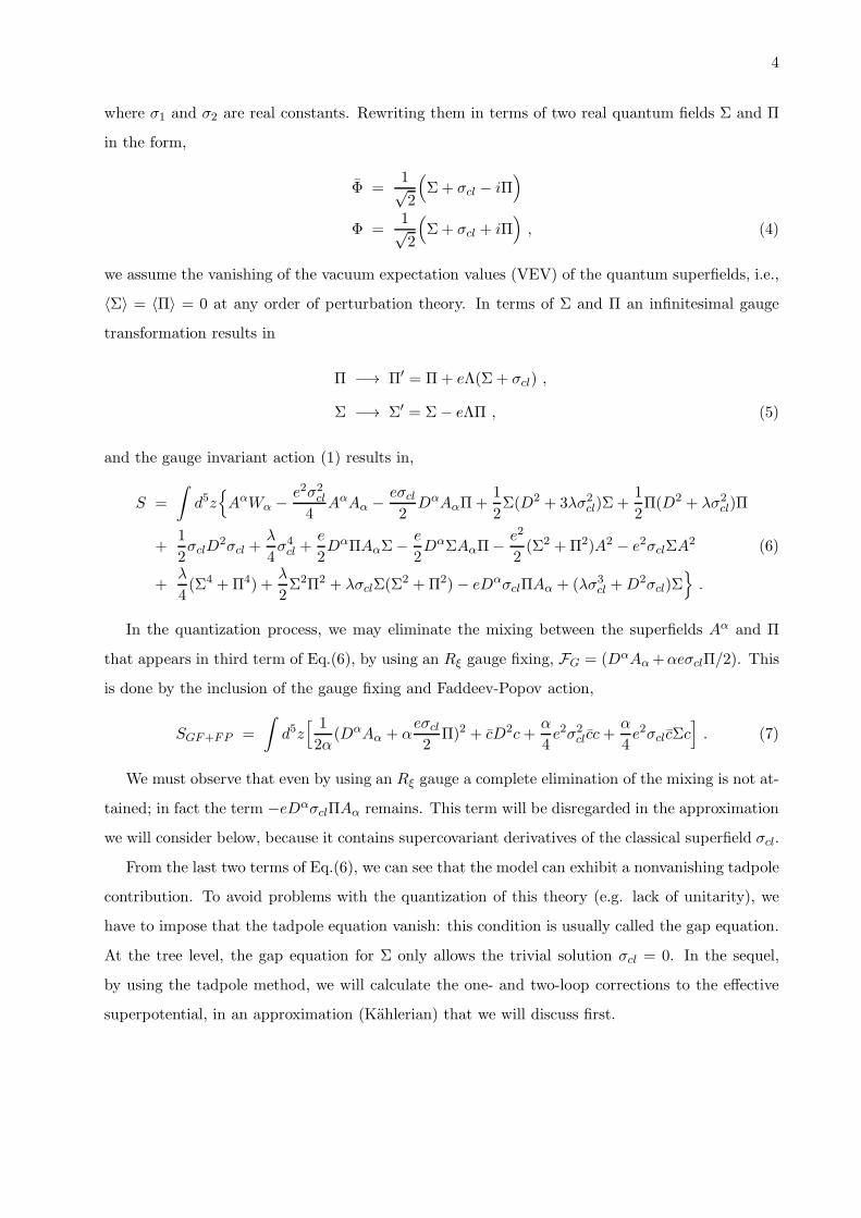
where σ1 and σ2 are real constants. Rewriting them in terms of two real quantum fields Σ and Π

in the form,

Φ =1√2

(

Σ+ σcl − iΠ)

Φ =1√2

(

Σ+ σcl + iΠ)

, (4)

we assume the vanishing of the vacuum expectation values (VEV) of the quantum superfields, i.e.,

〈Σ〉 = 〈Π〉 = 0 at any order of perturbation theory. In terms of Σ and Π an infinitesimal gauge

transformation results in

Π −→ Π′ = Π+ eΛ(Σ + σcl) ,

Σ −→ Σ′ = Σ− eΛΠ , (5)

and the gauge invariant action (1) results in,

S =

∫

d5z{

AαWα − e2σ2cl4

AαAα − eσcl2DαAαΠ+

1

2Σ(D2 + 3λσ2cl)Σ +

1

2Π(D2 + λσ2cl)Π

+1

2σclD

2σcl +λ

4σ4cl +

e

2DαΠAαΣ− e

2DαΣAαΠ− e2

2(Σ2 +Π2)A2 − e2σclΣA

2 (6)

+λ

4(Σ4 +Π4) +

λ

2Σ2Π2 + λσclΣ(Σ

2 +Π2)− eDασclΠAα + (λσ3cl +D2σcl)Σ}

.

In the quantization process, we may eliminate the mixing between the superfields Aα and Π

that appears in third term of Eq.(6), by using an Rξ gauge fixing, FG = (DαAα+αeσclΠ/2). This

is done by the inclusion of the gauge fixing and Faddeev-Popov action,

SGF+FP =

∫

d5z[ 1

2α(DαAα + α

eσcl2

Π)2 + cD2c+α

4e2σ2clcc+

α

4e2σclcΣc

]

. (7)

We must observe that even by using an Rξ gauge a complete elimination of the mixing is not at-

tained; in fact the term −eDασclΠAα remains. This term will be disregarded in the approximation

we will consider below, because it contains supercovariant derivatives of the classical superfield σcl.

From the last two terms of Eq.(6), we can see that the model can exhibit a nonvanishing tadpole

contribution. To avoid problems with the quantization of this theory (e.g. lack of unitarity), we

have to impose that the tadpole equation vanish: this condition is usually called the gap equation.

At the tree level, the gap equation for Σ only allows the trivial solution σcl = 0. In the sequel,

by using the tadpole method, we will calculate the one- and two-loop corrections to the effective

superpotential, in an approximation (Kahlerian) that we will discuss first.

5

From Eq.(6), the zero loop effective action Γcl, the superpotential Vcl, the Kahlerian superpo-

tential Kcl and the scalar potential Ucl can be seen to be given by

Γ[σcl] = −∫

d5z Vcl =

∫

d5z

[

1

2σclD

2σcl −Kcl(σcl )

]

= −∫

d3x Ucl =

∫

d3x

[

1

2σ22 − σ2

dKcl

dσcl(σ1)

]

(8)

where Kcl(σcl) = −λ4σ4cl and σ2

dKcl

dσ(σ1) = −λσ2σ31. After the elimination of the auxiliary field σ2

the scalar potential at classical level is given by: U0eff =

λ2

2σ61 .

As we are working in an explicit supersymmetric formulation, the radiative corrections to the

action and effective superpotential will be of the form [27]

Γrc[σcl] = −∫

d5z Vrc = −∫

d5z[

Krc(σcl) + F (DασclDασcl, D2σcl, σcl)

]

, (9)

whereKrc(σcl), a function of σcl but not of its derivatives, stands for the radiative corrections to the

Kahlerian effective superpotential, and F stands for the radiative corrections explicitly involving

at least a derivative of the classical field σcl. After integrating in d2θ we get for Γrc :

Γrc[σcl] = −∫

d3xUrc = −∫

d3x

[

σ2dKrc

dσ1(σ1) + σ22f(σ1, σ2)

]

(10)

where in the second term we made explicit the fact that the contributions coming from the F term

start at least with two powers of σ2.

From Eq.(8), Eq.(9) and Eq.(10), we have for the effective superpotential and the effective scalar

potential:

Veff (σcl) = −1

2σclD

2σcl + F (DασclDασcl, D2σcl, σcl) +K(σcl)

Ueff (σ1, σ2) = −1

2σ22 + σ22f(σ1, σ2) + σ2

dK

dσ1(σ1) , (11)

where K = Kcl +Krc. The vacuum of the model is determined by the equations:

0 =∂Ueff

∂σ1= σ2

d2K

dσ21(σ1) + σ22

∂f

∂σ1(σ1, σ2), (12)

0 =∂Ueff

∂σ2= −σ2 +

dK

dσ1(σ1) + 2σ2f(σ1, σ2) + σ22

∂f

∂σ2(σ2, σ2). (13)

For σ2 = 0 these equations result in Ueff (σ1, 0) = 0 at its minimum, signaling a supersymmetric

phase, and the condition:

0 =dK

dσ1(σ1). (14)

6

So, if a solution σ1 = v of this last equation exists, then Ueff (v, 0) = 0, and supersymmetry

is preserved. In short: the verification of the preservation of supersymmetry only requires the

knowledge of K(σcl). From now on we will restrict to its calculation, instead of the more involved

calculation of Veff (σcl).

To calculate K(σcl) it is enough to derive the Feynman rules from Eq.(6) and Eq.(7) by only

preserving the dependence in σ and dropping dependences in Dασ and D2σ, which also means, to

make the D-algebra operations by taking Dα(σX) = σDαX and D2(σX) = σD2X. In this way

the free propagators are given by:

〈T Σ(k, θ)Σ(−k, θ′)〉 = −iD2 −MΣ

k2 +M2Σ

δ(2)(θ − θ′) ,

〈T Π(k, θ)Π(−k, θ′)〉 = −iD2 −MΠ

k2 +M2Π

δ(2)(θ − θ′) , (15)

〈T Aα(k, θ)Aβ(−k, θ′)〉 =i

4

[(D2 +MA)D2DβDα

k2(k2 +M2A)

+ α(D2 − αMA)D

2DαDβ

k2(k2 + α2M2A)

]

δ(2)(θ − θ′) .

It is important to remark that the effective superpotential is a gauge-dependent quantity, as dis-

cussed in [28]. For simplicity, we will work in a supersymmetric Landau gauge, that is α = 0. With

this choice, the ghosts superfields decouple, and we can identify the “masses” of the interacting

superfields as

MΣ = 3λσ2cl, MΠ = λσ2cl , MA =e2σ2cl4

. (16)

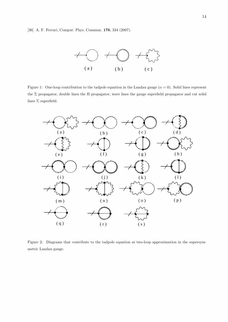
First, let us consider the one-loop corrections to the tadpole equation, which are drawn in Fig. 1.

The contributions at one-loop order, up to a common∫

d3p(2π)3

d2θΣ(p, θ) factor, can be written as

Γ(1)1l(a) = 3iλσcl

∫

d3k

(2π)31

k2 +M2Σ

, (17a)

Γ(1)1l(b) = iλσcl

∫

d3k

(2π)31

k2 +M2Π

, (17b)

Γ(1)1l(c) = i

e2

4σcl

∫

d3k

(2π)31

k2 +M2A

. (17c)

We will perform the integrals in Eq. (17) by using the regularization by dimensional reduction

[29]. This method of regularization has some advantages: first, one-loop graphs are finite; second,

two-loop divergences are a simple pole in ǫ = 3 − D; and third, starting with a Lagrangian with

only massless parameters, no dimensional parameters are generated (the µ parameter introduced

by the regularization will only appears in logarithms). This means, for example, that no mass

7

term of the form ΦΦ (which is not present in the unrenormalized Lagrangian) is generated by the

radiative corrections. For the tadpoles we get

Γ(1)(0+1)l = i

σ3cl4π

(

4πλ− 10λ2 − e4

16

)

. (18)

Setting Γ(1)(0+1)l = 0, we can see that the one-loop correction is not enough to ensure a nontrivial

solution to the gap equation, therefore no mass is generated in the first quantum approximation.

The same happens in the supersymmetric Maxwell theory [17], and nonsupersymmetric three-

dimensional gauge models [2–6].

Now, we evaluate the two-loop contributions to the tadpole equation, which arise from the

diagrams depicted in Fig. 2. Some details of this calculations are given in Appendix B. The

inclusion of such two-loop corrections in the tadpole equation leads to

Γ(1)(0+1+2)l = i σ3cl

[

b1 + b2 lnσ2clµ

]

+ iBσ3cl , (19)

where B is the counterterm, to be fixed later, µ is the mass scale introduced by the regularization,

b1 is a function of the coupling constants and 1/ǫ = 1/(3−D) (D is the dimension of the spacetime).

The quantity b2 is explicitly given by

b2 = −116 e6 + 543 e4λ+ 432e2λ2 − 71552 λ3

12288π2

≈ −(10−3) e6 − (4× 10−3) e4λ− (4× 10−3) e2λ2 + 0.6 λ3 . (20)

Let us evaluate the Kahlerian effective superpotential through the tadpole equation Eq.(24)

using the tadpole method [30–32] as in [19]. The Kahlerian effective superpotential is obtained

from the tadpole equation as K(σcl) = i∫

dσΓ(1), therefore the two-loop Kahlerian effective super-

potential is given by

K(σcl) = i

∫

dσclΓ(1)(0+1+2)l

= −b24σ4cl

(

b1b2

− 1

2+ ln

σ2clµ

)

− B

4σ4cl . (21)

The normalization of the Kahlerian effective superpotential, as usual, is defined in terms of the

tree-level coupling constant λ according to

λ

4≡ 1

4!

∂4K(σcl)

∂σ4cl

∣

∣

∣

σcl=v= − 1

12

(

3B + 3b1 + 11b2 + 3b2 lnv2

µ

)

, (22)

where v is the renormalization point; Eq.(22) fixes the counterterm B,

B = −b1 − λ− b2

(

11

3+ ln

v2

µ

)

. (23)

8

By substituting this counterterm in Eq.(19), the renormalized Kahlerian effective superpotential

can be cast as

K(σcl) = −b24σ4cl ln

[

σ2clv2

exp

(

λ

b2− 25

6

)]

. (24)

The minimum of the renormalized Kahlerian effective superpotential is at σcl = v that satisfies,

∂K(σcl)

∂σcl

∣

∣

∣

σcl=v= 0 , (25)

and a nontrivial minimum, with v 6= 0, requires the following constraint on the coupling constants,

λ =11

3b2 ≈ −(4× 10−3) e6 − (16× 10−3) e4λ− (13 × 10−3) e2λ2 + 2λ3. (26)

The compatibility of this relation with the assumptions of perturbation theory is the key

of Coleman-Weinberg mechanism. From Eq. (26), one can see that λ must be of order of

(4× 10−3)e6 +O(e10), thus for small e we are safely within the regime of validity of the perturba-

tive expansion. In a model with vanishing e, however, the dynamical gauge symmetry breaking is

incompatible with perturbation theory [1–6], because for e = 0 the Eq.(26) implies λ ∼ 1.

The mass term of matter superfield σcl is obtained as the second derivative of the renormalized

Kahlerian effective superpotential at its minimum. Using Eq.(26), we obtain

MΣ =d2K(σcl)

dσ2cl

∣

∣

∣

σcl=v≈ (2× 10−3)e6v2 , (27)

where the mass of the gauge superfield is given as

MA =e2

12λMΣ ≈ −250 e−4 . (28)

III. EXTENDED SUSY MODEL

A supersymmetric extension of the model defined in Eq.(1) to N = 2 can be obtained by

identifying the coupling constants as λ = −e2/8, plus some others generalizations that can be seen

in [22]. In particular, the N = 2 supersymmetric Chern-Simons action written in terms of N = 1

superfields was first obtained by Siegel [33]. Evaluating the quantum corrections discussed in the

previous section in this case, the Kahlerian effective superpotential can be expressed by

K(σcl) =c24e6σ4 log

{σ2

v2exp

(

1

c2e4− 25

6

)

}

, (29)

where c2 =519

32768π2≈ (1.6 × 10−3).

9

Now, studying a possible minimum of such a Kahlerian effective superpotential for v 6= 0, we

found that e2 ≈ (4.7× 10−2) e6, which implies e ∼ 2. Thus, as in other four and three-dimensional

scalar models [1–6], in this case the Coleman-Weinberg effect is not feasible, because for N = 2 the

model presents only one coupling constant into play. Our results are in agreement with previous

results obtained by Gaiotto and Yin [20] and Buchbinder et al. [21, 34], where it was shown that

the N = 2, 3 SCSM does not exhibit spontaneous breaking of superconformal invariance.

IV. CONCLUDING REMARKS

In this paper we studied the mechanism of dynamical breaking of gauge symmetry in a three-

dimensional supersymmetric model with classical superconformal invariance. Since we were work-

ing in an explicitly supersymmetric formalism, no breakdown of supersymmetry was detected, but

we show how the two-loop quantum corrections dynamically break the gauge and superconformal

invariances of the model, generating masses to the gauge and matter superfields. We also show

that, in the N = 2 extension of the model studied by us, the Coleman-Weinberg mechanism of

dynamical symmetry breaking is incompatible with perturbation theory, in agreement with the

results obtained by Gaiotto and Yin [20] and Buchbinder et al. [21].

One natural extension of our work would be to consider the possibility of supersymmetry break-

ing in the spirit of what was done for the Wess-Zumino model in [35], or through the component

formulation as in [18]. Another possibility is to study the effective superpotential for a noncom-

mutative extension of the present model, as done in [27].

Acknowledgments. This work was partially supported by the Brazilian agencies Conselho

Nacional de Desenvolvimento Cientıfico e Tecnologico (CNPq), Coordenacao de Aperfeicoamento

de Pessoal de Nıvel Superior (CAPES: AUX-PE-PROCAD 579/2008) and Fundacao de Amparo a

Pesquisa do Estado de Sao Paulo (FAPESP). A. Yu. P. has been supported by the CNPq Project

No. 303461-2009/8.

10

Appendix A: The expansions of superfields

A complex superfield can be written as the sum of real and imaginary parts as

Φ(x, θ) =1√2[Σ(x, θ) + iΠ(x, θ)] ,

Φ(x, θ) =1√2[Σ(x, θ)− iΠ(x, θ)] , (A1)

where the real scalar superfields can be expanded in terms of component fields as follows

Σ(x, θ) = σ(x) + θαψα(x)− θ2F (x) ,

Π(x, θ) = π(x) + θαξα(x)− θ2G(x) . (A2)

The spinorial superfield (gauge superfield), possess the following θ expansion

Aα(x, θ) = χα(x) + θβ [CαβB(x)− iVαβ(x)]− θ2 λα(x) , (A3)

and the associated field strength,

Wα =1

2DβDαAβ , (A4)

satisfies the Bianchi identity DαWα = 0. The component expansion of this field strength reads

Wα =1

2

(

∂αβχβ + λα

)

+ θβfβα − θ21

2

(

i∂αβλβ +�χα

)

, (A5)

where fαβ = (∂αλVλβ + ∂βλV

λα) is the 2-spinorial form of the Maxwell field strength FMN =

(∂MAN − ∂NAM ), M and N are the usual indices of the spacetime, which assume the values 0, 1

and 2.

Appendix B: Two-loop calculations

At two-loop, the contributions to the gap equation, associated with the diagrams depicted in

Fig. 2, are given by

Γ(1)2l(a) = i

3e2

2λσcl

∫

d3k

(2π)3d3q

(2π)3MΣ

(k2 +M2Σ)

2(q2 +M2A)

, (B1)

Γ(1)2l(b) = −18iλ2σcl

∫

d3k

(2π)3d3q

(2π)3MΣ

(k2 +M2Σ)

2(q2 +M2Σ)

, (B2)

Γ(1)2l(c) = −3iλ2σcl

∫

d3k

(2π)3d3q

(2π)3MΣ

(k2 +M2Σ)

2(q2 +M2Π)

, (B3)

11

Γ(1)2l(d) = −i3

4λ e2σcl

∫

d3k

(2π)3d3q

(2π)31

(k2 +M2Σ)

2[(k + q)2 +M2Π]q

2(q2 +M2A)

×[

M2ΣMA k · q − 2MAMΣMΠ k · q −MA k2 k · q − (MA +MΠ)M

2Σ q2

−(MA +MΠ − 2MΣ) q2 k2 + 2MΣ q2 k · q

]

, (B4)

Γ(1)2l(e) =

3i

16λe4σ3cl

∫

d3k

(2π)3d3q

(2π)31

k2(k2 +M2A)[(k + q)2 +M2

Σ]2q2(q2 +M2

A)

×[

M2ΣM

2A (k · q)−M2

A (k + q)2 (k · q)− 2MAMΣ (k · q) (k2 + q2)

+4MAMΣ k2 q2 +M2Σ k2 q2 − k2 q2 (k + q)2

]

, (B5)

Γ(1)2l(f) = −18iλ3σ3cl

∫

d3k

(2π)3d3q

(2π)35M2

Σ − k2

(k2 +M2Σ)

2[(k + q)2 +M2Σ](q

2 +M2Σ)

, (B6)

Γ(1)2l(g) = −6iλ3σ3cl

∫

d3k

(2π)3d3q

(2π)3M2

Σ + 4MΣMΠ − k2

(k2 +M2Σ)

2[(k + q)2 +M2Π](q

2 +M2Π)

, (B7)

Γ(1)2l(h) = −ie

2

2λσcl

∫

d3k

(2π)3d3q

(2π)3MΠ

(k2 +M2Π)

2(q2 +M2A)

, (B8)

Γ(1)2l(i) = −2iλ2σcl

∫

d3k

(2π)3d3q

(2π)3MΠ

(k2 +M2Π)

2(q2 +M2Σ)

, (B9)

Γ(1)2l(j) = −6iλ2σcl

∫

d3k

(2π)3d3q

(2π)3MΠ

(k2 +M2Π)

2(q2 +M2Π)

, (B10)

Γ(1)2l(k) =

i

4λe2σcl

∫

d3k

(2π)3d3q

(2π)31

(k2 +M2Π)

2[(k + q)2 +M2Σ]q

2(q2 +M2A)

×[

MAMΠ(2MΣ −MΠ) k · q −MA (k · q) k2 −M2Π(MA +MΣ) q

2

−2MΠ q2 k · q + (MA +MΣ − 2MΠ) k2 q2

]

, (B11)

Γ(1)2l(l)

= −4i

3λ3σ3cl

∫

d3k

(2π)3d3q

(2π)33MΠ + 2MΠMΣ − k2

(k2 +M2Π)

2(q2 +MΠ)[(k + q)2 +MΣ], (B12)

Γ(1)2l(m)

= ie4

8σcl

∫

d3k

(2π)3d3q

(2π)31

k2(k2 +M2A)

2[(k + q)2 +M2Π](q

2 +M2Σ)

×[

M2A(MΠ −MΣ) k · q −MΣMA(MA + 2MΠ) k

2

+(MΣ − 2MA −MΠ) (k · q) k2 +MΣ (k2)2 − 2MA k2 q2]

, (B13)

12

Γ(1)2l(n) = − i

96e6σ3cl

∫

d3k

(2π)3d3q

(2π)31

k2(k2 +M2A)

2[(k + q)2 +M2Σ]q

2(q2 +M2A)

×[

M3AMΣ k · q − (k2)2 q2 −MA(MΣ +MA) k · q k2

−M2A k · q q2 −MA(3MA + 2MΣ) k

2 q2 + (k · q) k2 q2]

, (B14)

Γ(1)2l(o) = i

e4

16σcl

∫

d3k

(2π)3d3q

(2π)3MA

(k2 +M2A)

2(q2 +M2Σ)

, (B15)

Γ(1)2l(p) = i

e4

16σcl

∫

d3k

(2π)3d3q

(2π)3MA

(k2 +M2A)

2(q2 +M2Π)

, (B16)

Γ(1)2l(q) = −9iλ2σcl

∫

d3k

(2π)3d3q

(2π)3MΣ

(k2 +M2Σ)(q

2 +M2Σ)[(k − q)2 +M2

Σ], (B17)

Γ(1)2l(r) = −4i

3λ2σcl

∫

d3k

(2π)3d3q

(2π)3MΣ + 2MΠ

(k2 +M2Σ)(q

2 +M2Π)[(k − q)2 +M2

Π], (B18)

Γ(1)2l(s) = −i e

4

16σcl

∫

d3k

(2π)3d3q

(2π)3M2

AMΣ k · q −MA(k2 + q2) k · q − (2MA +MΣ) k

2 q2

k2(k2 +M2A)q

2(q2 +M2A)[(q − k)2 +M2

Σ],(B19)

where the D-algebra manipulations on the two-loop supergraphs were performed with the help of

SusyMath [36], a MATHEMATICA c© package for supergraph calculations.

Performing the integrals in Eqs. (B1-B19) with the help of formulas [2–4], adopting the regular-

ization by dimensional reduction [29], and adding up the classical, one and two-loop contributions,

we obtain the following one point function,

Γ(1)(0+1+2)l = i σ3cl

[

b1 + b2 lnσ2clµ

]

, (B20)

where µ is a mass scale introduced by the regularization,

b2 = −116 e6 + 543 e4λ+ 432e2λ2 − 71552 λ3

12288π2

≈ −(10−3) e6 − (4 × 10−3) e4λ− (4× 10−3) e2λ2 + 0.6 λ3, (B21)

and b1 is some function of coupling constants and 1/ǫ = 1/(3−D) (D is the dimension of spacetime).

[1] S. R. Coleman and E. Weinberg, Phys. Rev. D 7, 1888 (1973).

[2] P. N. Tan, B. Tekin and Y. Hosotani, Phys. Lett. B 388, 611 (1996).

[3] P. N. Tan, B. Tekin and Y. Hosotani, Nucl. Phys. B 502, 483 (1997).

13

[4] A. G. Dias, M. Gomes and A. J. da Silva, Phys. Rev. D 69, 065011 (2004).

[5] V. S. Alves, M. Gomes, S. L. V. Pinheiro and A. J. da Silva, Phys. Rev. D 61, 065003 (2000).

[6] L. C. de Albuquerque, M. Gomes and A. J. da Silva, Phys. Rev. D 62, 085005 (2000).

[7] S. Deser, R. Jackiw and S. Templeton, Ann. Phys. (N.Y.)140, 372 (1982); 185, 406(E) (1988); 281,

409(E) (2000).

[8] J. A. Schonfeld, Nuclear Phys. B 185, 157 (1981).

[9] “The Quantum Hall Effect”, Graduate Texts in Contemporary Physics, R.E. Prange and S.M. Girvin

eds, Springer-Verlag, Berlin, 1990.

[10] J. H. Schwarz, JHEP 0411, 078 (2004).

[11] M. A. Bandres, A. E. Lipstein and J. H. Schwarz, JHEP 0805, 025 (2008).

[12] O. Aharony, O. Bergman, D. L. Jafferis and J. Maldacena, JHEP 0810, 091 (2008).

[13] J. Bagger and N. Lambert, Phys. Rev. D 75, 045020 (2007).

[14] J. Bagger and N. Lambert, Phys. Rev. D 77, 065008 (2008).

[15] A. Gustavsson, Nucl. Phys. B 811, 66 (2009).

[16] O. Miskovic and J. Zanelli, Phys. Rev. D 80, 044003 (2009).

[17] C. P. Burgess, Nucl. Phys. B 216, 459 (1983).

[18] A. C. Lehum, Phys. Rev. D 77, 067701 (2008).

[19] A. C. Lehum, Phys. Rev. D 79, 025005 (2009).

[20] D. Gaiotto and X. Yin, JHEP 0708, 056 (2007).

[21] I. L. Buchbinder, N. G. Pletnev and I. B. Samsonov, “Effective action of three-dimensional extended

supersymmetric matter on gauge superfield background,” arXiv:1003.4806 [hep-th].

[22] C. K. Lee, K. M. Lee and E. J. Weinberg, Phys. Lett. B 243, 105 (1990).

[23] S. J. J. Gates and H. Nishino, Phys. Lett. B 281, 72 (1992).

[24] H. Nishino and S. J. J. Gates, Int. J. Mod. Phys. A 8, 3371 (1993).

[25] S. J. Gates, M. T. Grisaru, M. Rocek and W. Siegel, Front. Phys. 58, 1 (1983).

[26] A. C. Lehum, A. F. Ferrari, M. Gomes and A. J. da Silva, Phys. Rev. D 76, 105021 (2007).

[27] A. F. Ferrari, M. Gomes, A. C. Lehum, J. R. Nascimento, A. Y. Petrov, E. O. Silva and A. J. da Silva,

Phys. Lett. B 678, 500 (2009).

[28] R. Jackiw, Phys. Rev. D 9, 1686 (1974).

[29] W. Siegel, Phys. Lett. B 84, 193 (1979).

[30] S. Weinberg, Phys. Rev. D 7, 2887 (1973).

[31] R. D. C. Miller, Nucl. Phys. B 228, 316 (1983).

[32] R. D. C. Miller, Nucl. Phys. B 229, 189 (1983).

[33] W. Siegel, Nucl. Phys. B 156, 135 (1979).

[34] I. L. Buchbinder, E. A. Ivanov, O. Lechtenfeld, N. G. Pletnev, I. B. Samsonov and B. M. Zupnik, JHEP

0910, 075 (2009).

[35] A. Amariti and M. Siani, JHEP 0908, 055 (2009)

14

[36] A. F. Ferrari, Comput. Phys. Commun. 176, 334 (2007).

( a ) ( b ) ( c )

Figure 1: One-loop contribution to the tadpole equation in the Landau gauge (α = 0). Solid lines represent

the Σ propagator, double lines the Π propagator, wave lines the gauge superfield propagator and cut solid

lines Σ superfield.

( a ) ( b ) ( c ) ( d )

( e ) ( f ) ( g ) ( h )

( i ) ( j ) ( k ) ( l )

( m ) ( n ) ( o ) ( p )

( q ) ( s )( r )

Figure 2: Diagrams that contribute to the tadpole equation at two-loop approximation in the supersym-

metric Landau gauge.