arXiv:1006.3395v1 [nlin.PS] 17 Jun 2010 Coherently coupled bright optical solitons and their collisions T. Kanna 1 , M. Vijayajayanthi 2 , and M. Lakshmanan 2 1 Post-Graduate and Research Department of Physics, Bishop Heber College, Tiruchirapalli–620 017, India 2 Centre for Nonlinear Dynamics, School of Physics, Bharathidasan University, Tiruchirapalli–620 024, India E-mail: kanna [email protected](corresponding author) E-mail: [email protected] Abstract. We obtain explicit bright one- and two-soliton solutions of the integrable case of the coherently coupled nonlinear Schr¨odinger equations by applying a non- standard form of the Hirota’s direct method. We find that the system admits both degenerate and non-degenerate solitons in which the latter can take single hump, double hump, and flat-top profiles. Our study on the collision dynamics of solitons in the integrable case shows that the collision among degenerate solitons and also the collision of non-degenerate solitons are always standard elastic collisions. But the collision of a degenerate soliton with a non-degenerate soliton induces switching in the latter leaving the former unaffected after collision, thereby showing a different mechanism from that of the Manakov system. PACS numbers: 02.30.Ik, 05.45.Yv

Welcome message from author
This document is posted to help you gain knowledge. Please leave a comment to let me know what you think about it! Share it to your friends and learn new things together.
Transcript
arX
iv:1
006.
3395
v1 [
nlin
.PS]
17
Jun
2010
Coherently coupled bright optical solitons and their
collisions
T. Kanna1, M. Vijayajayanthi2, and M. Lakshmanan2
1 Post-Graduate and Research Department of Physics, Bishop Heber College,
Tiruchirapalli–620 017, India2 Centre for Nonlinear Dynamics, School of Physics, Bharathidasan University,
Tiruchirapalli–620 024, India
E-mail: kanna [email protected](corresponding author)
E-mail: [email protected]
Abstract. We obtain explicit bright one- and two-soliton solutions of the integrable
case of the coherently coupled nonlinear Schrodinger equations by applying a non-
standard form of the Hirota’s direct method. We find that the system admits both
degenerate and non-degenerate solitons in which the latter can take single hump, double
hump, and flat-top profiles. Our study on the collision dynamics of solitons in the
integrable case shows that the collision among degenerate solitons and also the collision
of non-degenerate solitons are always standard elastic collisions. But the collision of a
degenerate soliton with a non-degenerate soliton induces switching in the latter leaving
the former unaffected after collision, thereby showing a different mechanism from that
of the Manakov system.
PACS numbers: 02.30.Ik, 05.45.Yv
Coherently coupled bright optical solitons and their collisions 2
1. Introduction
Recently there has been considerable interest in studying the dynamics of
multicomponent solitons/solitary waves in view of their wide range of applications
encompassing science and engineering [1, 2]. In the context of nonlinear optics,
simultaneous propagation of multiple optical pulses or beams in nonlinear media is
governed by a class of multicomponent nonlinear Schrodinger (NLS) type equations
which is non-integrable in general. These multicomponent NLS equations fall into
two categories, namely incoherently coupled NLS equations and coherently coupled
NLS equations [1]. The integrable as well as non-integrable incoherently coupled NLS
equations have been well studied in the literature [1, 3]. Particularly, the studies on
integrable Manakov system [4], a two component nonlinear system with incoherent
coupling, and also its integrable N-component generalization [4–7], have revealed the
fact that the bright solitons of these systems exhibit interesting collision scenario which
is not possible in their single component counterparts. This collision behaviour has been
exploited in the construction of logic gates based on optical soliton collisions [8, 9] and
also such collisions lead to the possibility of multi-state logic [7, 10].
The set of coherently coupled NLS systems is another interesting class of nonlinear
evolution equations for which much attention is yet to be paid. The term coherent
coupling here stands for the dependence of coupling on relative phases of the interacting
fields. A fairly general governing equation for coherently coupled orthogonally polarized
waveguide modes in the Kerr medium (see for example, Sec. 9.4.1 in ref. [1]) is
iq1,Z + δq1,TT − µq1 + (|q1|2 + σ|q2|2)q1 + λq22q∗1 = 0,
iq2,Z + δq2,TT + µq2 + (σ|q1|2 + |q2|2)q2 + λq21q∗2 = 0, (1)
where Z and T are the propagation direction and the transverse direction, respectively,
q1 and q2 are slowly varying complex amplitudes in each polarization mode, µ is
the degree of birefringence, σ is the incoherent coupling parameter and λ is the
coherent coupling parameter. Similar equations also arise in the context of short
pulse propagation in weakly birefringent Kerr type nonlinear media [1, 2], where the
co-ordinate T corresponds to retarded time. In general the system (1) is non-integrable.
An integrable non-dimensional coherently coupled NLS equation closely associated with
equation (1) can be written as
iq1z − q1tt − γ(|q1|2 + 2|q2|2)q1 − γq22q∗1 = 0,
iq2z − q2tt − γ(2|q1|2 + |q2|2)q2 − γq21q∗2 = 0. (2)
The above set of equations results from equation (1) for the choice µ = 0 (low
birefringence limit), σ = 2, λ = 1, a choice which is possible in a cubic anisotropic
nonlinear medium where the parameters λ and σ can be chosen separately but their ratio
is fixed as σλ= 2 [1,2] and by performing the transformations T →
√γδ t and Z → −γz,
where γ > 0. Although the physical conditions for the above choice are stringent to
obtain, we hope the exact results reported in this paper will serve as potential candidates
in further analysis of the non-integrable coherently coupled NLS equations (1), which
Coherently coupled bright optical solitons and their collisions 3
have received attention recently [11–14].
Motivated by the above considerations, in this paper we have obtained general
soliton solutions of system (2) by applying a non-conventional form of Hirota’s
bilinearization method [15]. Another integrable equation which can also be obtained
from equation (1), having a form similar to equation (2) but with the replacement of
the ‘−’ sign appearing before the coherent coupling term by a ‘+’ sign with γ = 1,
has been studied in refs. [11, 12] and special one- and two-soliton solutions with less
number of parameters have been obtained by applying the Hirota’s direct method. In
fact, while obtaining the two-soliton solution by a linear superposition as reported in
ref. [12], following the lines of ref. [11], the governing equation gets decoupled into
two independent NLS equations and so the information regarding the coherent and
incoherent coupling terms gets lost. This system can also be studied by applying a
similar method as developed here and the results will be published separately. The
main objective of this paper is to obtain an appropriate bilinear form of equation (2)
resulting in more general soliton solutions as done in ref. [16] for the Sasa-Satsuma higher
order NLS system. We also wish to investigate the soliton formation and propagation
due to the combined effects of self phase modulation (SPM), cross phase modulation
(XPM) and coherent coupling between the copropagating fields. Our study shows that
there exist two distinct type of solitons, namely degenerate and non-degenerate solitons,
where the non-degenerate solitons can have single and double hump profiles. Their
collision behaviour is also fascinating. Particularly, the collision between degenerate
and non-degenerate solitons shows a different kind of switching mechanism in the two
component system (2) from that of the shape changing collisions occurring in the
Manakov system [5, 7].
This paper is organized in the following manner. The non-standard way of obtaining
the bilinear equations of the integrable system (2) by introducing an auxiliary function
is discussed in section 2. The general one-soliton solution is obtained in section 3 and
the degenerate and non-degenerate solitons are discussed. In section 4, the more general
two-soliton solution reflecting the effects of coherent coupling terms during collision is
obtained. The collisions of degenerate solitons and non-degenerate solitons are discussed
separately in section 5 and we have also analysed the collision of a degenerate soliton with
a non-degenerate soliton in the same section. Final section 6 is allotted for conclusion.
2. A non-standard bilinearization method for the coherently coupled NLS
system
The soliton solutions of system (2) can be obtained by applying the Hirota’s
bilinearization method [15], which is a powerful tool for integrable nonlinear partial
differential equations. To obtain the correct bilinear equations, resulting in more general
soliton solutions displaying the effects of SPM, XPM, and coherent coupling, we adopt
a non-standard method by introducing an auxiliary function, similar to the technique
followed by Gilson et al [16] for the higher order NLS system. By performing the
Coherently coupled bright optical solitons and their collisions 4
bilinearizing transformation
q1 =g
fand q2 =
h
f, (3)
to equation (2) and introducing an auxiliary function s, we obtain the following set of
bilinear equations,
D1 g · f = −γsg∗, D1 h · f = γsh∗, (4a)
D2 f · f = 2γ(
|g|2 + |h|2)
, sf = g2 − h2, (4b)
where D1 = iDz − D2t , D2 = D2
t , g and h are complex functions, while f is a real
function, ∗ denotes the complex conjugate and the Hirota’s bilinear operators Dz and
Dt are defined as [15]
DpzD
qt (a · b) =
( ∂
∂z− ∂
∂z′
)p( ∂
∂t− ∂
∂t′
)q
a(z, t)b(z′, t′)|(z = z′, t = t′). (5)
Note that the necessity for the introduction of an auxiliary function s(z, t) becomes
crucial as otherwise in the absence of s in equation (4), only special cases of even one-
soliton solution reported below will be obtained and for higher order solitons severe
constraints on the soliton parameters will arise. The above set of equations (4) can be
solved by introducing the following power series expansions for g, h, f , and s:
g = χg1 + χ3g3 + . . . , h = χh1 + χ3h3 + . . . , (6a)
f = 1 + χ2f2 + χ4f4 + . . . , s = χ2s2 + χ4s4 + . . . , (6b)
where χ is the formal power series expansion parameter. The resulting set of linear
partial differential equations, after collecting the terms with the same powers in χ, can
be solved recursively to obtain the forms of g, h, f , and s.
3. Bright one-soliton solutions
In order to obtain the one-soliton solution, unlike in the Manakov case [5, 6], here
we restrict the power series expansion (6) as g = χg1 + χ3g3, h = χh1 + χ3h3,
f = 1 + χ2f2 + χ4f4, s = χ2s2. After introducing this series expansion in equation
(4) and by solving the resulting set of linear partial differential equations recursively,
one can obtain the explicit one-soliton solution as
q1 =α1e
η1 + e2η1+η∗
1+δ11
1 + eη1+η∗
1+R1 + e2η1+2η∗1+ǫ11, (7a)
q2 =β1e
η1 + e2η1+η∗
1+ρ11
1 + eη1+η∗
1+R1 + e2η1+2η∗1+ǫ11, (7b)
where the auxiliary function takes the form
s = (α21 − β2
1)e2η1 . (7c)
Here
η1 = k1(t− ik1z), eδ11 =γα∗
1(α21 − β2
1)
2(k1 + k∗1)
2, eρ11 =
−γβ∗1(α
21 − β2
1)
2(k1 + k∗1)
2, (7d)
eR1 =γ(|α1|2 + |β1|2)
(k1 + k∗1)
2, eǫ11 =
γ2(α21 − β2
1)(α∗21 − β∗2
1 )
4(k1 + k∗1)
4. (7e)
Coherently coupled bright optical solitons and their collisions 5
Case(i): α21 − β2
1 = 0
This choice α21 − β2
1 = 0 always results in the standard “sech” profile for the bright
soliton solution (7). It can be expressed as
q1 =(α1
2e−
R12
)
sech
(
η1R +R1
2
)
eiη1I ≡ A1sech
(
η1R +R1
2
)
eiη1I , (8)
and q2 = ±q1 corresponding to β1 = ±α1 so that |q1|2 = |q2|2. Here A1 =(
α1
2e−
R12
)
,
R1 = log(
2γ|α1|2
(k1+k∗1)2
)
, and η1 = η1R + iη1I , where η1R = k1R(t + 2k1Iz) and η1I =
k1It+(k21I−k2
1R)z. Throughout this paper the subscripts R and I represent the real and
imaginary parts, respectively. We call the solitons arising for the choice α21 − β2
1 = 0 as
degenerate solitons, owing to the fact that such solitons posses the same intensity profile
in both the components q1 and q2 and are characterized by two complex parameters
α1 and k1 or four real parameters, instead of the six real parameters in the Manakov
case [7]. Here A1, −2k1I , andR1
2k1Rare the amplitude, velocity, and central position of the
soliton, respectively. Note that A1
k1Ris related to the polarization of the pulse/beam. The
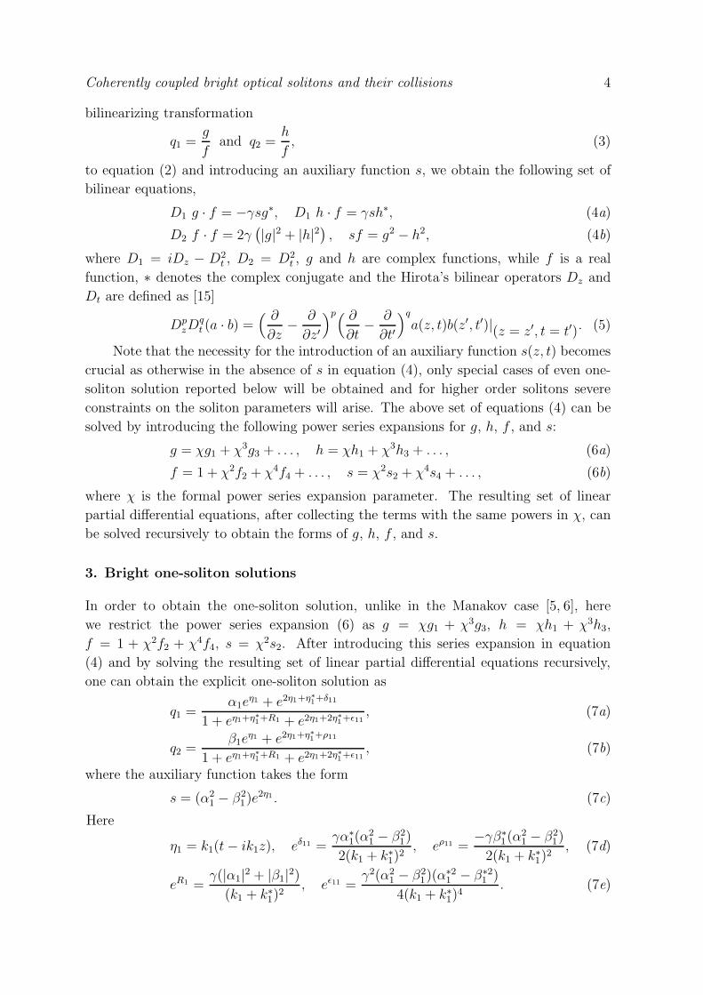
degenerate soliton having a single hump profile is depicted in figure 1 for the parameters
γ = 2, k1 = 1 + i, and α1 = β1 = 1 at t = 0.
Figure 1. Degenerate one-soliton at t = 0 (parameters are as given in the text).
Note that in the present case, since α21 − β2
1 = 0, the auxiliary function s vanishes,
see equation (7c), and so from the bilinear equations (4) one can easily infer that the
effect of coherent coupling vanishes.
Case(ii): α21 − β2
1 6= 0
The nature of soliton for the other choice α21 − β2
1 6= 0, can be understood by
rewriting q1 and q2 in the expression (7) as
qj =2Aj
[
cos(Pj)cosh(
η1R + ǫ114
)
+ i sin(Pj)sinh(
η1R + ǫ114
)]
eiη1I
4cosh2(
η1R + ǫ114
)
+ L, j = 1, 2, (9)
where A1 = e(l1+δ11−ǫ11
2 ), A2 = e(l2+ρ11−ǫ11
2 ), P1 = (δ11I−l1I )2
, P2 = (ρ11I−l2I )2
, L =
e(R1−ǫ112 ) − 2, η1R = k1R(t + 2k1Iz), η1I = k1It + (k2
1I − k21R)z, l1 = ln(α1), and
Coherently coupled bright optical solitons and their collisions 6
l2 = ln(β1). Also, the quantities δ11, ρ11, R1, and ǫ11 are as defined in equation (7). Here
Aj represents the amplitude of the soliton in the j-th component and for this case by the
term amplitude we mean the peak value of the soliton profile. The speed of the soliton
is given by 2k1I and its central position is ǫ114k1R
. It can be noticed that by rewriting
the expression (9) for the choice α1 = β1, it reduces to equation (8). The general form
presented here will be of use in the asymptotic analysis of the two-soliton and multi-
soliton solutions. We refer to the above soliton as non-degenerate due to their distinct
intensity profiles in the q1 and q2 components. In contrast to the degenerate solitons
these solitons can vary their profile from a single hump to a double hump through a flat-
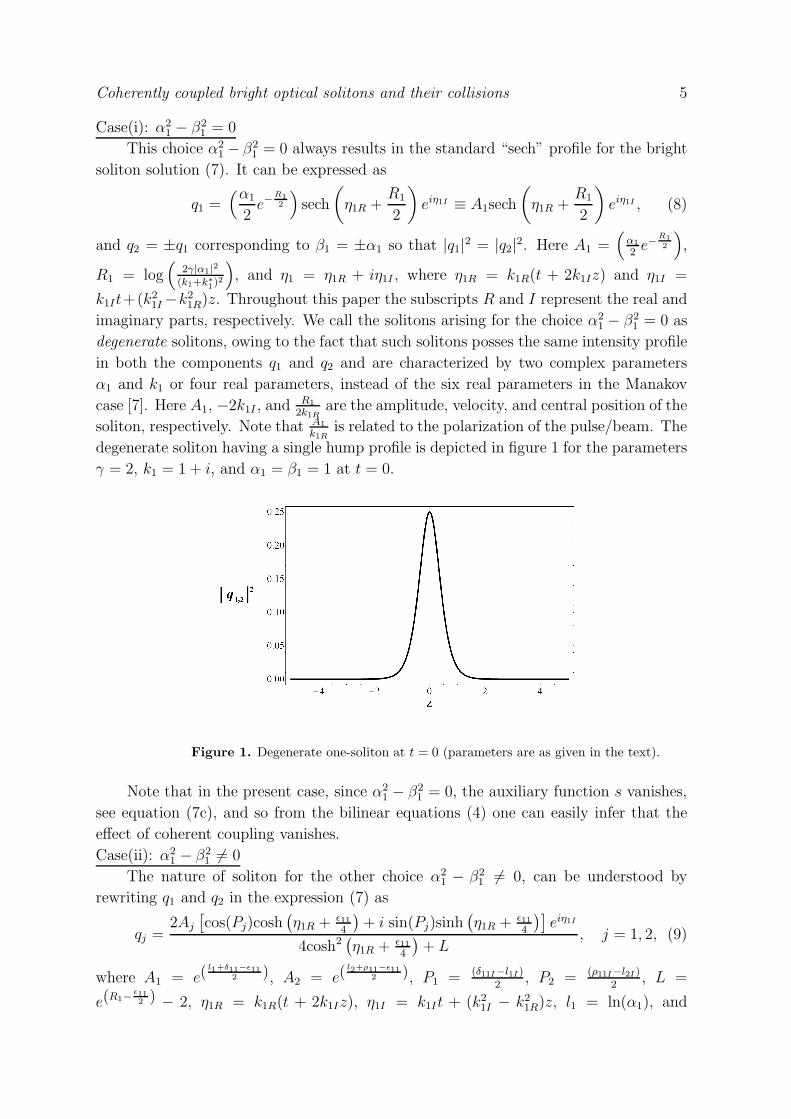
top profile as the parameters are varied. A double hump soliton and a flat-top soliton
appearing in the q1 and q2 components, respectively, at t = 0 are shown in figure 2 for
the parameters γ = 2, k1 = 1 + i, α1 = 0.7114, and β1 = 1. Similar kind of flat-top
Figure 2. A non-degenerate soliton at t = 0: (a) Double hump non-degenerate
soliton in the q1 component. (b) Flat-top non-degenerate soliton in the q2 component
(parameters are as given in the text).
structures have been reported in complex Ginzburg-Landau equation [2]. Note that in
equation (9) also the standard sech type soliton occurs for a particular choice of the
parameters, namely α1β∗1 + α∗
1β1 = 0, for which P1, P2, and L become zero in equation
Coherently coupled bright optical solitons and their collisions 7
(9). However, in the present case, the effect of coherent coupling does not vanish unlike
the case of degenerate solitons.
It can be noticed that equation (2) is embedded into the matrix NLS equation which
is integrable via Inverse Scattering Transform (IST) method [17, 18]. Cases (i) and (ii)
have also been reported in refs. [17, 18] for a three component version of the equation
considered in this paper by applying the results of the IST method for the matrix
NLS equation and the corresponding solutions were referred as ferromagnetic and polar
solitons, respectively, in the context of multicomponent spinor condensates. Here we
have obtained similar kind of more general soliton solutions for the two component case
itself by applying a non-standard type of Hirota’s bilinearization method.
4. Bright two-soliton solution
The two-soliton solution of the system (2) can be obtained after terminating the
power series (6) as g = χg1 + χ3g3 + χ5g5 + χ7g7, h = χh1 + χ3h3 + χ5h5 + χ7h7,
f = 1 + χ2f2 + χ4f4 + χ6f6 + χ8f8, s = χ2s2 + χ4s4 + χ6s6 and again by solving the
resultant linear partial differential equations recursively. Then the explicit form of the
two-soliton solution can be written as
qj =N (j)
D, j = 1, 2. (10a)
The functions N (1), N (2) and D in (10a) are given by the expressions
N (1) = α1eη1 + α2e
η2 + e2η1+η∗
1+δ11 + e2η1+η∗
2+δ12 + e2η2+η∗
1+δ21 + e2η2+η∗
2+δ22
+ eη1+η∗
1+η2+δ1 + eη2+η∗
2+η1+δ2 + e2η1+2η∗1+η2+µ11 + e2η1+2η∗2+η2+µ12
+ e2η2+2η∗1+η1+µ21 + e2η2+2η∗2+η1+µ22 + e2η1+η∗
1+η2+η∗
2+µ1
+ e2η2+η∗
2+η1+η∗
1+µ2 + e2η1+2η∗1+2η2+η∗2+φ1 + e2η1+2η2+2η∗2+η∗
1+φ2 , (10b)
N (2) = β1eη1 + β2e
η2 + e2η1+η∗
1+ρ11 + e2η1+η∗
2+ρ12 + e2η2+η∗
1+ρ21 + e2η2+η∗
2+ρ22
+ eη1+η∗
1+η2+ρ1 + eη2+η∗
2+η1+ρ2 + e2η1+2η∗1+η2+ν11 + e2η1+2η∗2+η2+ν12
+ e2η2+2η∗1+η1+ν21 + e2η2+2η∗2+η1+ν22 + e2η1+η∗
1+η2+η∗
2+ν1
+ e2η2+η∗
2+η1+η∗
1+ν2 + e2η1+2η∗1+2η2+η∗2+ψ1 + e2η1+2η2+2η∗2+η∗
1+ψ2, (10c)
D = 1 + eη1+η∗
1+R1 + eη1+η∗
2+δ0 + eη2+η∗
1+δ∗
0 + eη2+η∗
2+R2 + e2η1+2η∗1+ǫ11
+ e2η1+2η∗2+ǫ12 + e2η2+2η∗1+ǫ21 + e2η2+2η∗2+ǫ22 + e2η1+η∗
1+η∗
2+τ1
+ e2η∗
1+η1+η2+τ∗
1 + e2η2+η∗
1+η∗
2+τ2 + e2η∗
2+η1+η2+τ∗
2 + eη1+η∗
1+η2+η∗
2+R3
+ e2η1+2η∗1+η2+η∗
2+θ11 + e2η1+2η∗2+η2+η∗
1+θ12 + e2η2+2η∗1+η1+η∗
2+θ21
+ e2η2+2η∗2+η1+η∗
1+θ22 + e2(η1+η∗
1+η2+η∗
2)+R4 , (10d)
and the auxiliary function s is determined as
s = (α21 − β2
1)e2η1 + (α2
2 − β22)e
2η2 + 2(α1α2 − β1β2)eη1+η2 + eη1+η
∗
1+2η2+λ11
+ eη1+η∗
2+2η2+λ12 + eη2+η∗
1+2η1+λ21 + eη2+η∗
2+2η1+λ22 + e2η1+2η∗1+2η2+λ1
+ e2η1+2η2+2η∗2+λ2 + e2η1+η∗
1+2η2+η∗2+λ3. (10e)
Coherently coupled bright optical solitons and their collisions 8
Here ηi = ki(t − ikiz), i = 1, 2. The real and imaginary parts of ηj are given by
ηjR = kjR(t+2kjIz) and ηjI = kjIt+(k2jI−k2
jR)z, j = 1, 2. Various quantities appearing
in equation (10) are given in the Appendix, as they are rather lengthy expressions. In
order to understand the structure of the above two-soliton solution, we now perform
an asymptotic analysis and analyse the nature of the soliton collisions in the present
system.
5. Collision of solitons
The two-soliton solution obtained in the previous section represents the interaction of
two solitons. It is of interest to consider the collision among non-degenerate solitons and
degenerate solitons, and also the collision between the non-degenerate and degenerate
solitons. For this purpose we perform the asymptotic analysis of the two-soliton solution
(10) by considering the case where k1R, k2R > 0 and k1I > k2I , without loss of generality.
The analysis is straightforward for the other choices of kjR and kjI , j = 1, 2.
5.1. Collision of non-degenerate solitons (α2j 6= β2
j , j = 1, 2)
The asymptotic forms of S1 and S2 before collision (z → −∞) and after collision
(z → +∞) can be deduced from equation (10) as follows. The quantities ηjR and ηjI ,
j = 1, 2, appearing in the following asymptotic expressions are defined below equation
(10).
1. Before Collision (z → −∞)
Soliton S1 (η1R ≃ 0, η2R → −∞):(
q1−1q1−2
)
≃ 1
D1
(
A1−1 0
0 A1−2
)(
cos(P1) i sin(P1)
cos(P2) i sin(P2)
)(
cosh(η−1R)
sinh(η−1R)
)
eiη1I , (11a)
where(
A1−1
A1−2
)
= 2e−(R4+ǫ22)
2
(
e(µ22+φ2)
2
e(ν22+ψ2)
2
)
, (11b)
D1 = 4 cosh2(η−1R) + e
(
θ22−(R4+ǫ22)
2
)
− 2. (11c)
In the above, P1 = φ2I−µ22I2
, P2 = ψ2I−ν22I2
, and η−1R = η1R + R4−ǫ224
. Here and in the
following the superscript denotes the soliton and the subscript denotes the component
and - (+) sign appearing in the superscript represents the asymptotic form of the soliton
before (after) interaction.
Soliton S2 (η2R ≃ 0, η1R → ∞):(
q2−1q2−2
)
≃ 1
D2
(
A2−1 0
0 A2−2
)(
cos(Q1) i sin(Q1)
cos(Q2) i sin(Q2)
)(
cosh(η−2R)
sinh(η−2R)
)
eiη2I , (12a)
where
Coherently coupled bright optical solitons and their collisions 9
(
A2−1
A2−2
)
= 2e−ǫ222
el−
1 +δ222
el−
2+ρ222
, (12b)
D2 = 4 cosh2(η−2R) + e(R2−ǫ222 ) − 2. (12c)
Here, Q1 =δ22I−l
−
1I
2, Q2 =
ρ22I−l−
2I
2, l−1 = ln(α2), l
−2 = ln(β2), and η−2R = η2R + ǫ22
4. All the
quantities appearing in the above asymptotic expressions (11) and (12) are defined in
the Appendix.
2. After Collision:
The asymptotic expressions after collision are similar to those of before collision
expressions with the replacement of Aj−l and η−jR by A
j+l and η+jR, respectively for the
soliton Sj, j = 1, 2, where A1+l =
(k1+k∗2)(k∗
1−k∗
2)
(k∗1+k2)(k1−k2)A1−l , A2+
l =(k1+k∗2)(k1−k2)
(k∗1+k2)(k∗
1−k∗
2)A2−l , l = 1, 2,
η+1R = η1R + ǫ114, and η+2R = η2R + (R4−ǫ11)
4. The quantities ǫ11 and R4 are given in
the Appendix. One can easily check that the intensities before and after interaction
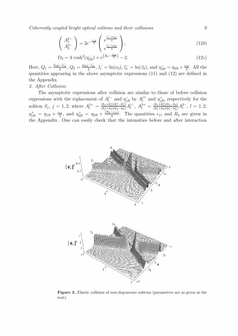
Figure 3. Elastic collision of non-degenerate solitons (parameters are as given in the
text).
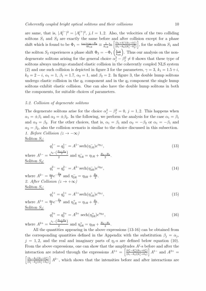
Coherently coupled bright optical solitons and their collisions 10
are same, that is, |Aj−l |2 = |Aj+
l |2, j, l = 1, 2. Also, the velocities of the two colliding
solitons S1 and S2 are exactly the same before and after collision except for a phase
shift which is found to be Φ1 =ǫ11+ǫ22−R4
4k1R≡ 1
k1Rln[
(k2+k∗1)(k1+k∗
2)
(k1−k2)(k∗1−k∗
2)
]
, for the soliton S1 and
the soliton S2 experiences a phase shift Φ2 = −Φ1
(
k1Rk2R
)
. Thus our analysis on the non-
degenerate solitons arising for the general choice α2j − β2
j 6= 0 shows that these type of
solitons always undergo standard elastic collision in the coherently coupled NLS system
(2) and one such collision is depicted in figure 3 for the parameters, γ = 3, k1 = 1.5+ i,
k2 = 2− i, α1 = 1, β1 = 1.7, α2 = 1, and β2 = 2. In figure 3, the double hump solitons
undergo elastic collision in the q1 component and in the q2 component the single hump
solitons exhibit elastic collision. One can also have the double hump solitons in both
the components, for suitable choices of parameters.
5.2. Collision of degenerate solitons
The degenerate solitons arise for the choice α2j − β2
j = 0, j = 1, 2. This happens when
α1 = ±β1 and α2 = ±β2. In the following, we perform the analysis for the case α1 = β1
and α2 = β2. For the other choices, that is, α1 = β1 and α2 = −β2 or α1 = −β1 and
α2 = β2, also the collision scenario is similar to the choice discussed in this subsection.
1. Before Collision (z → −∞)
Soliton S1:
q1−1 = q1−2 = A1−sech(η−1R)eiη1I , (13)
where A1− = eδ2−(R2+R3
2 )2
and η−1R = η1R + R3−R2
2.
Soliton S2:
q2−1 = q2−2 = A2−sech(η−2R)eiη2I , (14)
where A2− = α2
2e−
R22 and η−2R = η2R + R2
2.
2. After Collision (z → +∞)
Soliton S1:
q1+1 = q1+2 = A1+sech(η+1R)eiη1I , (15)
where A1+ = α1
2e−
R12 and η+1R = η1R + R1
2.
Soliton S2:
q2+1 = q2+2 = A2+ sech(η+2R)eiη2I , (16)
where A2+ = eδ1−(R1+R3
2 )2
and η+2R = η2R + R3−R1
2.
All the quantities appearing in the above expressions (13-16) can be obtained from
the corresponding quantities defined in the Appendix with the substitution βj = αj ,
j = 1, 2, and the real and imaginary parts of ηj-s are defined below equation (10).
From the above expressions, one can show that the amplitudes Aj-s before and after the
interaction are related through the expressions A1+ =[
(k∗1−k∗
2)(k1+k∗
2)
(k1−k2)(k∗1+k2)
]
A1− and A2+ =[
(k1−k2)(k1+k∗2)
(k∗1−k∗
2)(k∗
1+k2)
]
A2−, which shows that the intensities before and after interactions are
Coherently coupled bright optical solitons and their collisions 11
the same, that is |Aj+|2 = |Aj−|2, j = 1, 2. Also the soliton S1 undergoes a phase shift
Φ1 =R1+R2−R3
2k1R, whereas the soliton S2 experiences a phase shift Φ2 = −Φ1
(
k1Rk2R
)
during
collision. Thus the degenerate solitons always undergo standard elastic collision as that
of the NLS solitons.
5.3. Collision between degenerate and non-degenerate solitons
The collision of a degenerate soliton (α2j − β2
j = 0) with a non-degenerate soliton
(α2j−β2
j 6= 0) exhibits very interesting collision properties. Here we consider the collision
of a non-degenerate soliton S1 (α1 6= β1) with a degenerate soliton S2 (α2 = β2). Note
that the analysis can also be performed for the other possible choices like α2 = −β2,
but here also one can infer the same kind of collision scenario as for the present choice
α2 = β2. The asymptotic forms of the solitons S1 and S2 are presented below.
1. Before Collision
Soliton S1:(
q1−1q1−2
)
=1
D1−
(
A1−1 0
0 A1−2
)(
cos(P−1 ) i sin(P−
1 )
cos(Q−1 ) i sin(Q−
1 )
)(
cosh(η−1R)
sinh(η−1R)
)
eiη1I , (17)
where
(
A1−1
A1−2
)
= 2
(
eδ2+µ1−θ11−R2
2
eρ2+ν1−θ11−R2
2
)
, D1− = 4cosh2(η−1R) + L1−, P−1 = δ2I−µ1I
2,
Q−1 = ρ2I−ν1I
2, η−1R = η1R+
θ11−R2
4, and L1− = e
(
R3−(θ11+R2)
2
)
−2. Note that the expressions
for various quantities appearing in equation (17) and in the equations (18-20) given below
can be obtained from the corresponding quantities defined in the Appendix by putting
β2 = α2.
Soliton S2:
q2−1 = q2−2 = A2−sech(η−2R)eiη2I , (18)
where A2− = α2
2e−
R22 and η−2R = η2R + R2
2.
2. After Collision
Soliton S1:(
q1+1q1+2
)
=1
D1+
(
A1+1 0
0 A1+2
)(
cos(P+1 ) i sin(P+
1 )
cos(Q+1 ) i sin(Q+
1 )
)(
cosh(η+1R)
sinh(η+1R)
)
eiη1I , (19)
where P+1 =
δ11I−l+1I
2, Q+
1 =ρ11I−l
+2I
2, D1+ = 4cosh2(η+1R) +L1+, l+1I = ln(α1), l
+2I = ln(β1),
η+1R = η1R + ǫ114, and L1+ = eR1−
ǫ112 − 2. The amplitudes A1+
1 and A1+2 are given by the
relations A1+1 = T1 A1−
1 and A1+2 = T2 A1−
2 . Here the transition amplitude
T1 =
√
4(k∗1 − k∗
2)2(k1 + k∗
2)2α1α
∗1
|[(k1 − k2)2 + (k1 + k∗2)
2]α1 + (k2 − k∗2 − 2k1)(k2 + k∗
2)β1|2(20)
and the expression for T2 can be obtained by replacing α1 ↔ β1 and α∗1 ↔ β∗
1 in the
expression for T1.
Soliton S2:
q2+1 ≡ q2+2 = A2+sech(η+2R)eiη2I , (21)
Coherently coupled bright optical solitons and their collisions 12
where A2+ =(k1−k2)(k1+k∗2)
(k∗1−k∗
2)(k∗
1+k2)A2− and η+2R = η2R+ θ11−ǫ11
2. The real and imaginary parts of
ηj-s appearing in the above expressions are already defined below equation (10).
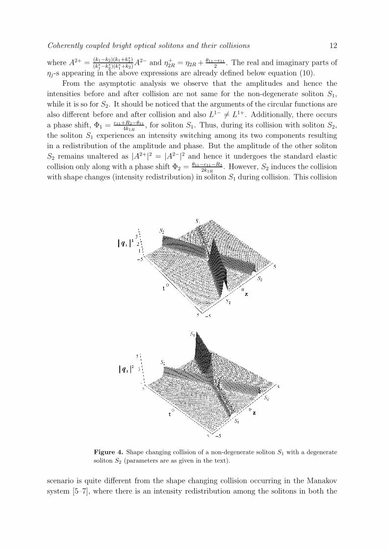
From the asymptotic analysis we observe that the amplitudes and hence the
intensities before and after collision are not same for the non-degenerate soliton S1,
while it is so for S2. It should be noticed that the arguments of the circular functions are
also different before and after collision and also L1− 6= L1+. Additionally, there occurs
a phase shift, Φ1 =ǫ11+R2−θ11
4k1R, for soliton S1. Thus, during its collision with soliton S2,
the soliton S1 experiences an intensity switching among its two components resulting
in a redistribution of the amplitude and phase. But the amplitude of the other soliton
S2 remains unaltered as |A2+|2 = |A2−|2 and hence it undergoes the standard elastic
collision only along with a phase shift Φ2 =θ11−ǫ11−R2
2k1R. However, S2 induces the collision
with shape changes (intensity redistribution) in soliton S1 during collision. This collision
Figure 4. Shape changing collision of a non-degenerate soliton S1 with a degenerate
soliton S2 (parameters are as given in the text).
scenario is quite different from the shape changing collision occurring in the Manakov
system [5–7], where there is an intensity redistribution among the solitons in both the
Coherently coupled bright optical solitons and their collisions 13
components but in the present system it happens only among the two components of
the non-degenerate soliton S1. Note that though the total energy of both the solitons
is conserved independently due to the conservation law,∫ +∞
−∞(|q1|2 + |q2|2)dt=constant,
the energy of the soliton in the individual modes that is∫ +∞
−∞|q1|2dt and
∫ +∞
−∞|q2|2dt
are not conserved independently as the soliton S1 only experiences intensity switching
in both the components. It could be an interesting future study to check whether |Tj|,j = 1, 2, can be unimodular, if so, for what choices of α-s and β-s this will happen.
For illustrative purpose, the above collision scenario is shown in figure 4 for the
parameters γ = 2, k1 = 2.3 + i, k2 = 2.5 − i, α1 = 0.75, β1 = 1.9, and α2 = β2 = 3 + i.
The figure shows that in the q1 component the single hump soliton S1 changes its profile
to a double hump soliton and also experiences significant suppression in its intensity
whereas the soliton S2 undergoes elastic collision. The reverse scenario takes place for
the soliton S1 in the q2 component and here also the soliton S2 remains unaltered after
collision.
In the collision of non-degenerate solitons alone the coherent coupling modifies
uniformly both the solitons before and after collision, thereby resulting in an elastic
collision. But in the present case the effect of coherent coupling is switched off in the
degenerate soliton S2 (since α22 = β2
2), however the coupling still persists in the non-
degenerate soliton S1. Hence, along with the XPM term the coherent coupling influences
the non-degenerate soliton S1 resulting in an intensity switching during collision. From
a mathematical point of view, one finds that the asymptotically dominant terms of the
non-degenerate soliton collision case become insignificant and the less dominant terms
in that case become significant in the two-soliton solution expression corresponding
to the collision of a degenerate soliton with a non-degenerate one. This yields different
asymptotic expressions for these two collision processes as seen in the present subsection
and in section 5.1, which ultimately makes their collision scenario completely different.
6. Conclusion
Explicit forms of one- and two-soliton solutions of the coherently coupled NLS equations
have been obtained using a non-standard type of Hirota’s bilinearization method.
Analysing the nature of the bright one-soliton solution we have reported degenerate
solitons (solitons possessing same intensity in the q1 and q2 components) and non-
degenerate solitons (solitons with different intensities in the q1 and q2 components).
Particularly, for non-degenerate solitons the density profile can vary from single hump
to double hump profile including flat-top solitons. Our analysis on the collision dynamics
revealed the fact that separate collisions among degenerate solitons alone or among non-
degenerate solitons alone are elastic. On the other hand, collision of a degenerate soliton
with a non-degenerate soliton exhibits nontrivial behaviour resulting in an intensity
switching of the non-degenerate soliton spread up in the two components leaving the
other soliton unaltered. This property will have immediate applications in soliton
collision based computing. Apart from the switching, we have also observed that this
Coherently coupled bright optical solitons and their collisions 14
collision transforms the soliton profile from single hump to double hump including flat-
top profile or vice versa. We expect that this property can find application in pulse
shaping in the context of nonlinear optics.
The above analysis can be extended to the study of three and higher order soliton
solutions. The details of multi-soliton collisions and the multicomponent cases will be
published separately.
Acknowledgements
TK acknowledges the support of the Department of Science and Technology,
Government of India under the DST Fast Track Project for young scientists. TK
also thanks the Principal and Management of Bishop Heber College, Tiruchirapalli,
for constant support and encouragement. The works of MV and ML are supported by
a DST-IRPHA project. ML is also supported by DST Ramanna Fellowship.
References
[1] Kivshar Y S and Agrawal G P 2003 Optical Solitons: From Fibers to Photonic Crystals (San Diego:
Academic Press)
[2] Akhmediev N and Ankiewicz A 1997 Solitons: Nonlinear Pulses and Beams (London: Chapman
and Hall)
[3] Ablowitz M J, Prinari B and Trubatch A D 2004 Discrete and Continuous Nonlinear Schrodinger
Systems (Cambridge: Cambridge University Press)
[4] Manakov S V 1973 Zh. Eksp. Teor. Fiz. 65 505 [1974 Sov. Phys. JETP 38 248]
[5] Radhakrishnan R, Lakshmanan M and Hietarinta J 1997 Phys. Rev. E 56 2213
[6] Kanna T and Lakshmanan M 2001 Phys. Rev. Lett. 86 5043
[7] Kanna T and Lakshmanan M 2003 Phys. Rev. E 67 046617
[8] Jakubowski M H, Steiglitz K and Squier R 1998 Phys. Rev. E 58 6752
[9] Steiglitz K 2000 Phys. Rev. E 63 016608
[10] Ablowitz M J, Prinari B and Trubatch A D 2004 Inverse Probl. 20 1217
[11] Park Q H and Shin H J 1999 Phys. Rev. E 59 2373
[12] Zhang H Q, Xu T, Li J and Tian B 2008 Phys. Rev. E 77 026605
[13] Chiu H S and Chow K W 2009 Phys. Rev. A 79 065803
[14] Brainis E 2009 Phys. Rev. A 79 023840
[15] Hirota R 2004 The Direct Method in Soliton Theory (Cambridge: Cambridge University Press)
[16] Gilson C, Hietarinta J, Nimmo J and Ohta Y 2003 Phys. Rev. E 68 016614
[17] Ieda J, Miyakawa T and Wadati M 2004 Phys. Rev. Lett. 93 194102
[18] Ieda J, Miyakawa T and Wadati M 2004 J. Phys. Soc. Jpn. 73 2996
Appendix
The various quantities occurring in equation (10) and in section 5 have the following
forms:
eδij =α∗j (α
2i − β2
i )γ
2(ki + k∗j )
2, eδj =
(α∗j (α1α2 − β1β2)γ + (k1 − k2)(α1κ2j − α2κ1j))
(kj + k∗j )(k3−j + k∗
j ),
Coherently coupled bright optical solitons and their collisions 15
eρij = −β∗j
α∗j
eδij , eρj =(β∗
j (−α1α2 + β1β2)γ + (k1 − k2)(β1κ2j − β2κ1j))
(kj + k∗j )(k3−j + k∗
j ),
eµij =(k1 − k2)
2α3−i(α2i − β2
i )(α∗2j − β∗2
j )γ2
4(ki + k∗j )
4(k∗3−i + kj)2
, eνij =β3−i
α3−i
eµij
eRj =κjj
(kj + k∗j ), eδ0 =
κ12
(k1 + k∗2), eδ
∗
0 =κ21
(k2 + k∗1),
eφj =
(
γ3(k1 − k2)4(k∗
1 − k∗2)
2(α21 − β2
1)(α22 − β2
2)
8(kj + k∗j )
4(k3−j + k∗j )
4(kj + k∗3−j)
2(k3−j + k∗3−j)
2
)
α∗3−j(α
∗2j − β∗2
j ),
eψj = −β∗3−j
α∗3−j
eφj , eǫij =γ2(α2
i − β2i )(α
∗2j − β∗2
j )
4(ki + k∗j )
4,
eτj =γ2(α2
j − β2j )(α
∗1α
∗2 − β∗
1β∗2)
2(kj + k∗j )
2(kj + k∗3−j)
2, eτ
∗
j =γ2(α∗2
j − β∗2j )(α1α2 − β1β2)
2(kj + k∗j )
2(k∗j + k3−j)2
,
eµ1 =(k1 − k2)
2γ2(α21 − β2
1)
D
([
(k2 + k∗1)
2 + (k∗2 − k∗
1)(k∗2 + k2)
]
α2α∗1α
∗2
−(k∗1 − k∗
2)(k2 + k∗2)α
∗2β2β
∗1 + (k2 + k∗
1)(k∗1 − k∗
2)α∗1β2β
∗2 − (k2 + k∗
1)(k2 + k∗2)α2β
∗1β
∗2) ,
eµ2 =(k1 − k2)
2γ2(α22 − β2
2)
D
(
[(k1 + k∗1)
2 + (k∗2 − k∗
1)(k∗2 + k1)]α1α
∗1α
∗2
−(k∗1 − k∗
2)(k1 + k∗2)α
∗2β1β
∗1 + (k1 + k∗
1)(k∗1 − k∗
2)α∗1β1β
∗2 − (k1 + k∗
1)(k1 + k∗2)α1β
∗1β
∗2) ,
eν1 =−(k1 − k2)
2γ2(α21 − β2
1)
D
(
[(k2 + k∗1)
2 + (k∗2 − k∗
1)(k∗2 + k2)]β2β
∗1β
∗2
−(k∗1 − k∗
2)(k2 + k∗2)β
∗2α2α
∗1 + (k2 + k∗
1)(k∗1 − k∗
2)β∗1α2α
∗2 − (k2 + k∗
1)(k2 + k∗2)β2α
∗1α
∗2) ,
eν2 = − (k1 − k2)2γ2(α2
2 − β22)
D
(
[(k1 + k∗1)
2 + (k∗2 − k∗
1)(k∗2 + k1)]β1β
∗1β
∗2
−(k∗1 − k∗
2)(k1 + k∗2)β
∗2α1α
∗1 + (k1 + k∗
1)(k∗1 − k∗
2)β∗1α1α
∗2 − (k1 + k∗
1)(k1 + k∗2)β1α
∗1α
∗2) ,
eR3 = γ2[
(
(k∗1 + k2)
2(k1 + k∗2)
2 − (k1 + k∗1)(k
∗1 + k2)(k1 + k∗
2)(k2 + k∗2) + (k1 + k∗
1)2(k2 + k∗
2)2
(k1 + k∗1)
2(k∗1 + k2)2(k1 + k∗
2)2(k2 + k∗
2)2
)
(α1α∗1α2α
∗2 + β1β
∗1β2β
∗2) +
(
(k1 − k2)(k∗1 − k∗
2)(α2α∗2β1β
∗1 + α1α
∗1β2β
∗2)
(k1 + k∗1)
2(k∗1 + k2)(k1 + k∗
2)(k2 + k∗2)
2
)
−(
(α∗1α
∗2β1β2 + α1α2β
∗1β
∗2)
(k1 + k∗1)(k
∗1 + k2)(k1 + k∗
2)(k2 + k∗2)
)
−(
(k1 − k2)(k∗1 − k∗
2)(α1α∗2β2β
∗1 + α2α
∗1β1β
∗2)
(k1 + k∗1)(k
∗1 + k2)2(k1 + k∗
2)2(k2 + k∗
2)
)
]
,
eθij =(k1 − k2)
2(k∗1 − k∗
2)2(α2
i − β2i )(α
∗2j − β∗2
j )(α3−iα∗3−j + β3−iβ
∗3−j)γ
3
2D(ki + k∗j )
2,
eR4 =1
4D2(k1 − k2)
4(k∗1 − k∗
2)4(α2
1 − β21)(α
∗21 − β∗2
1 )(α22 − β2
2)(α∗22 − β∗2
2 )γ4,
eλij =(k1 − k2)
2(α23−i − β2
3−i)κijγ
(k3−i + k∗j )
2(ki + k∗j )
, eλj =γ2(k1 − k2)
4(α21 − β2
1)(α22 − β2
2)(α∗2j − β∗2
j )γ2
4(kj + k∗j )
4(k∗j + k3−j)4
,
eλ3 =1
D(k1 − k2)
4(α21 − β2
1)(α22 − β2
2)(α∗1α
∗2 − β∗
1β∗2)γ
2,
where
D = 2(k1 + k∗1)
2(k∗1 + k2)
2(k1 + k∗2)
2(k2 + k∗2)
2
Coherently coupled bright optical solitons and their collisions 16
and
κij =γ(αiα
∗j + βiβ
∗j )
(ki + k∗j )
, i, j = 1, 2.
Related Documents