Classification and Prediction: Regression Via Gradient Descent Optimization Bamshad Mobasher DePaul University Bamshad Mobasher DePaul University.

Classification and Prediction:Regression Via Gradient Descent

Optimization

Bamshad MobasherDePaul University

Bamshad MobasherDePaul University

2

Linear Regression

i Linear regression: involves a response variable y and a single predictor variable x y = w0 + w1 x

4 The weights w0 (y-intercept) and w1 (slope) are regression coefficients

i Method of least squares: estimates the best-fitting straight line4 w0 and w1 are obtained by minimizing the sum of the squared errors (a.k.a.

residuals)

ii

iii

xx

yyxxw

21 )(

))((

xwyw 10

210

22

))((

)ˆ(

ii

iii

ii

xwwy

yye

w1 can be obtained by setting the partial derivative of the SSE to 0 and solving for w1, ultimately resulting in:

3

Multiple Linear Regression i Multiple linear regression: involves more than one predictor variable

4 Features represented as x1, x2, …, xd

4 Training data is of the form (x1, y1), (x2, y2),…, (xn, yn) (each xj is a row vector in matrix X, i.e. a row in the data)

4 For a specific value of a feature xi in data item xj we use:

4 Ex. For 2-D data, the regression function is:

4 More generally:

x1 yx2

jix

22110y xwxww

xw .),...,(y T0

101

wxwwxxfd

iiid

i Multiple dimensions

4 To simplify add a new feature x0 = 1 to feature vector x:

Least Squares Generalization

yx2x1x0

11111

xw .),...,,(y T

010010

d

iii

d

iiid xwxwxwxxxf

4 Calculate the error function (SSE) and determine w:

Least Squares Generalization

testtesttest

j

j

y

y

xxw

yXXXw

xX

y

XwyXwy

samplefor test ˆ

)(

samples trainingall ofmatrix

responses trainingall ofvector

)()(

T1T

T

n

j

d

i

jii

id

iii xwyxwfE

1

2

0

2

0

2 )()()( yxyw

Closed form solution to

xwx .)(),...,,(y T

010010

d

iii

d

iiid xwxwxwfxxxf

0)(

ww

E

Gradient Descent Optimizationi Linear regression can also be solved using Gradient Decent

optimization approachi GD can be used in a variety of settings to find the minimum value

of functions (including non-linear functions) where a closed form solution is not available or not easily obtained

i Basic idea:4 Given an objective function J(w) (e.g., sum of squared errors), with w as a vector

of variables w0, w1, …, wd, iteratively minimize J(w) by finding the gradient of the function surface in the variable-space and adjusting the weights in the opposite direction

4 The gradient is a vector with each element representing the slope of the function in the direction of one of the variables

4 Each element is the partial derivative of function with respect to one of variables

6

dd w

f

w

f

w

fwwwJJ

)()()(),,,()(

2121

wwww

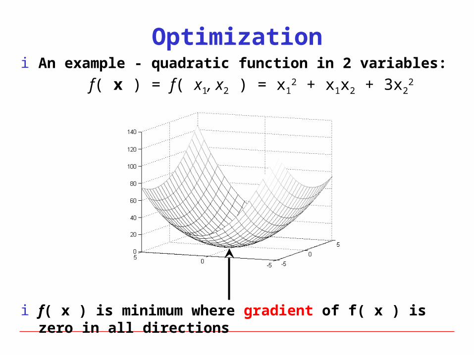
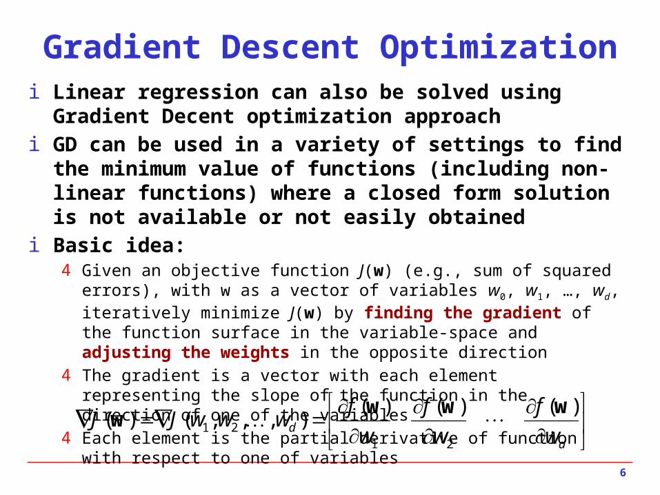
i An example - quadratic function in 2 variables:

f( x ) = f( x1, x2 ) = x12 + x1x2 + 3x2

2

i f( x ) is minimum where gradient of f( x ) is zero in all directions

Optimization

i Gradient is a vector4 Each element is the slope of function along direction of one of variables4 Each element is the partial derivative of function with respect to one of

variables

4 Example:

Optimization

212121

21

2221

2121

62)()(

),()(

3),()(

xxxxx

f

x

fxxff

xxxxxxff

xxx

x

Optimizationi Gradient vector points in direction of steepest ascent of function

121 ),( xxxf

),( 21 xxf

),( 21 xxf

221 ),( xxxf

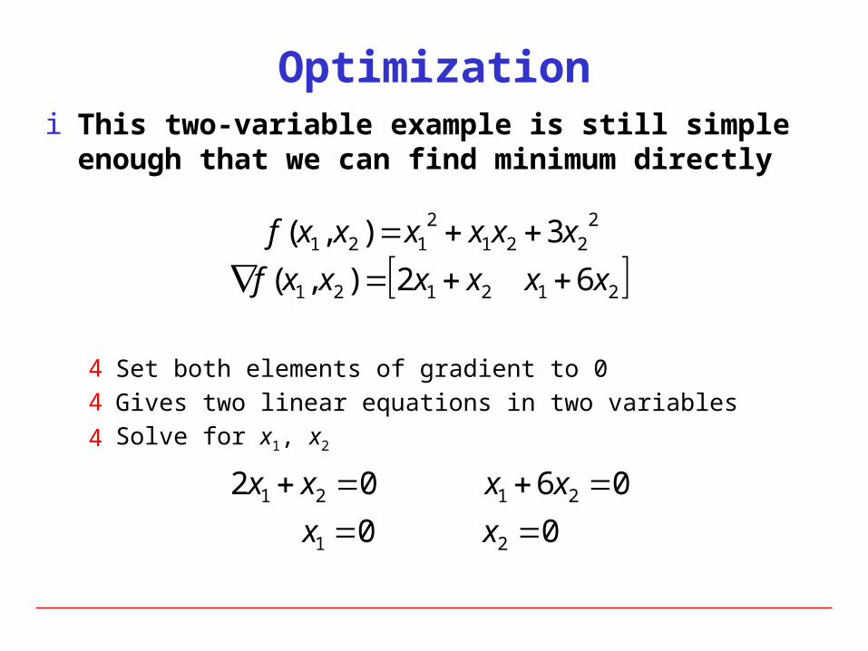
i This two-variable example is still simple enough that we can find minimum directly

4 Set both elements of gradient to 04 Gives two linear equations in two variables

4 Solve for x1, x2

Optimization

212121

2221

2121

62),(

3),(

xxxxxxf

xxxxxxf

0 0

06 02

21

2121

xx

xxxx

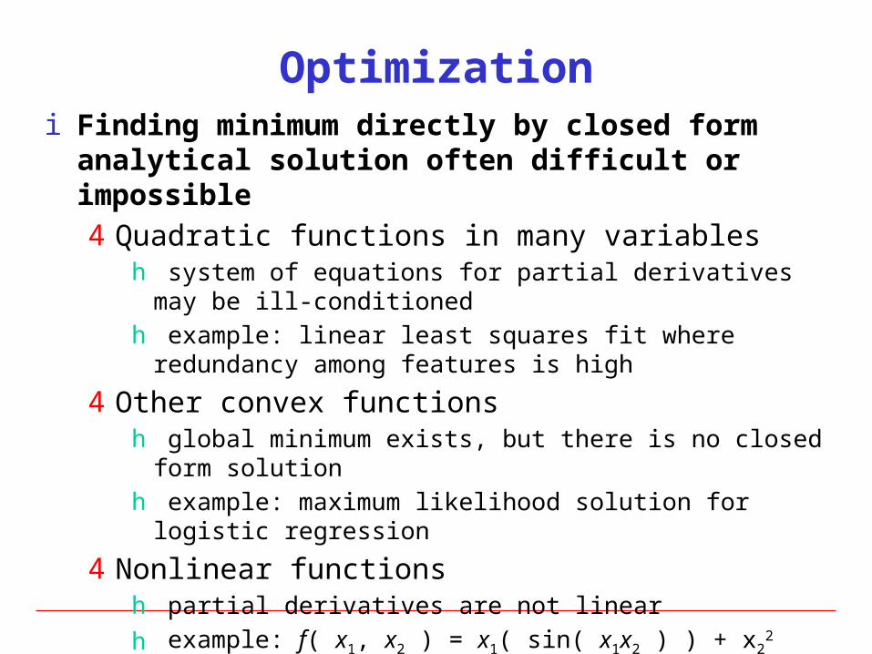
i Finding minimum directly by closed form analytical solution often difficult or impossible4 Quadratic functions in many variables

h system of equations for partial derivatives may be ill-conditionedh example: linear least squares fit where redundancy among features is

high

4 Other convex functionsh global minimum exists, but there is no closed form solutionh example: maximum likelihood solution for logistic regression

4 Nonlinear functionsh partial derivatives are not linear

h example: f( x1, x2 ) = x1( sin( x1x2 ) ) + x22

h example: sum of transfer functions in neural networks

Optimization

i Given an objective (e.g., error) function E(w) = E(w0, w1, …, wd)

i Process (follow the gradient downhill):

1. Pick an initial set of weights (random): w = (w0, w1, …, wd)

2. Determine the descent direction: -E(wt)

3. Choose a learning rate: 4. Update your position: wt+1 = wt - E(wt)5. Repeat from 2) until stopping criterion is satisfied

i Typical stopping criteria4 E( wt+1 ) ~ 04 some validation metric is optimized

Gradient descent optimization

Note: this step involves simultaneous updating of each weight wi

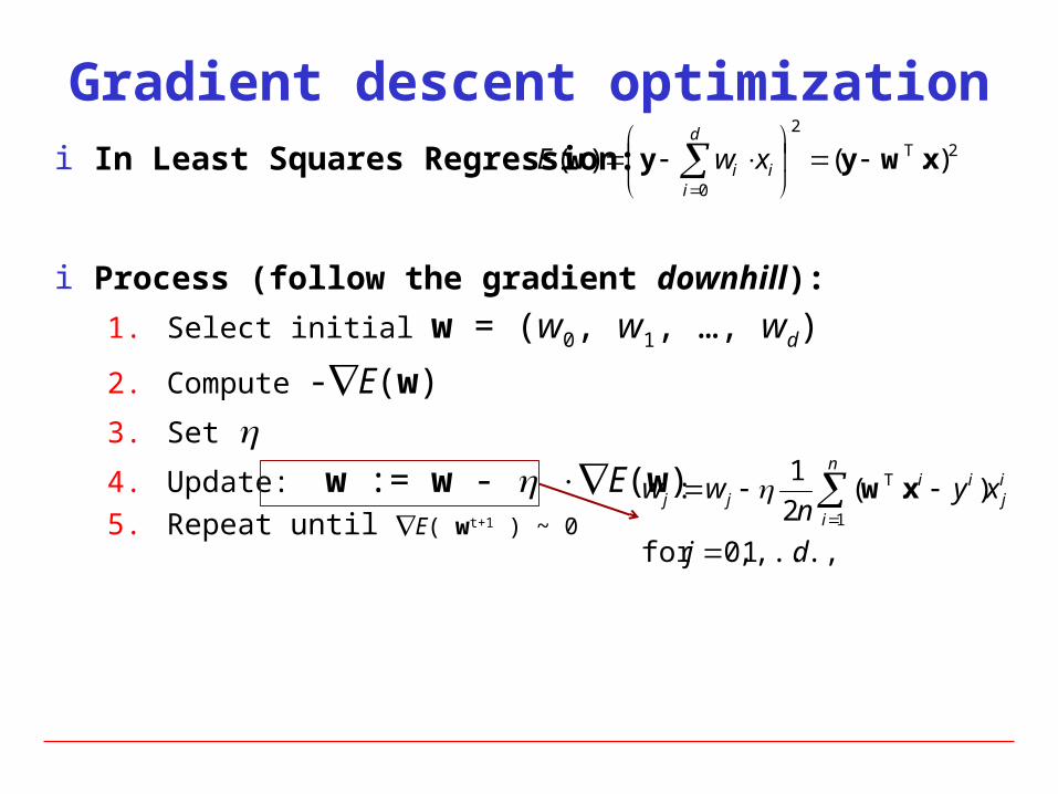
i In Least Squares Regression:

i Process (follow the gradient downhill):

1. Select initial w = (w0, w1, …, wd)

2. Compute -E(w)

3. Set 4. Update: w := w - E(w)5. Repeat until E( wt+1 ) ~ 0

Gradient descent optimization2T

2

0

).()( xwyyw

d

iii xwE

dj

xyn

ww ij

n

i

iijj

,...,1,0for

).(2

1:

1

T

xw

Illustration of Gradient Descent

w1

w0

E(w)

Illustration of Gradient Descent

w1

w0

E(w)

Illustration of Gradient Descent

w1

w0

E(w)

Direction of steepestdescent = direction ofnegative gradient

Illustration of Gradient Descent

w1

w0

E(w)

Original point inweight space

New point inweight space

i Problems:4 Choosing step size (learning rate)

h too small convergence is slow and inefficienth too large may not converge

4 Can get stuck on “flat” areas of function4 Easily trapped in local minima

Gradient descent optimization

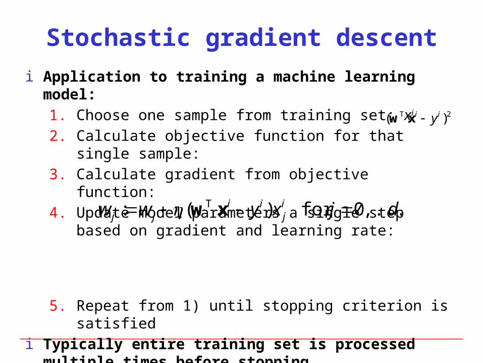
i Application to training a machine learning model:

1. Choose one sample from training set: xi

2. Calculate objective function for that single sample:

3. Calculate gradient from objective function:

4. Update model parameters a single step based on gradient and learning rate:

5. Repeat from 1) until stopping criterion is satisfiedi Typically entire training set is processed multiple times before

stoppingi Order in which samples are processed can be fixed or random.

Stochastic gradient descent

2T ).( ii yxw

djxyww ij

iijj ,...,0for ).(: T xw