Circumventing storage limitations in variational data assimilation studies

SIAM J. SCI. COMPUT. c 1995 Society for Industrial and Applied MathematicsVol. 1, No. 2, pp. 1{100, May 1995 002Circumventing Storage Limitationsin Variational Data Assimilation Studies�JUAN MARIO RESTREPOy GARY K. LEAFy and ANDREAS GRIEWANKzAbstract. An application of Pontryagin's Maximum Principle, data assimilation is used toblend possibly incomplete or nonuniformly distributed spatio-temporal observational data into geo-physical models. Used extensively in engineering control theory applications, data assimilation hasrelatively recently been introduced into meteorological forecasting, natural-resource recovery model-ing, and climate dynamics.Variational data assimilation is a promising assimilation technique in which it is assumed thatthe optimal state of the system is an extrema of a carefully chosen cost function. Provided that anadjoint model is available, the required model gradient can be computed by integrating the modelforward and its adjoint backward. The gradient is then used to extremize the cost function with asuitable iterative or conjugate gradient solver.The problem addressed in this study is the explosive growth in both on-line computer memoryand remote storage requirements of computing the gradient by the forward/adjoint technique whichcharacterize large-scale assimilation studies. Storage limitations impose severe limitation on the sizeof assimilation studies, even on the largest computers. By using a recursive strategy, a schedulecan be constructed that enables the forward/adjoint model runs to be performed in such a waythat storage requirements can be traded for longer computational times. This generally-applicablestrategy enables data assimilation studies on signi�cantly larger domains than would otherwise bepossible, given the particular hardware constraints, without compromising the outcome in any way.Furthermore, it is shown that this tradeo� is indeed viable and that when the schedule is optimized,the storage and computational times grow at most logarithmically.Key words. variational data assimilation, gradient, adjoint model, climate, meteorology, nat-ural resources recovery, recursion, storageAMS subject classi�cations. 86A05, 86A10, 86A22, 86-04, 86-08[1]. IntroductionData assimilation has relatively recently become an important tool in many ar-eas of geophysics, such as weather and climate forecasting [2,3,5,10,11,12,17], modelsensitivity analysis [14,15,20], and in the inclusion of �eld data sets into theoreticalmodel-studies [4,9,18]. In weather forecasting, �eld data that may be spatially and/ortemporally heteregeneous is blended into dynamical models as soon as the �eld datais available. As a result, the predictive capabilities of today's weather models haveimproved signi�cantly [11,16]. However, the practical use of data assimilation in some� The authors thank Eli Tziperman for making his climate code available to us. J.M.R. becameaware of this data assimilation problem in the course of many stimulating hours of conversation withJochem Marotzke from MIT and Kirk Bryan from GFDL; their patience and their hospitality aremuch appreciated. This research was supported in part by an appointment to the DistinguishedPost-doctoral Research Program sponsored by the U.S. Department of Energy, O�ce of University andScience Education Programs, and administered by the Oak Ridge Institute for Science and Educa-tion. Further support was provided by the Mathematical, Information, and Computational SciencesDivision subprogram of the O�ce of Computational and Technology Research, U.S. Department ofEnergy, under Contract W-31-109-Eng-38.yMathematics and Computer Science Division, Argonne National Laboratory, Argonne, IL60439 U.S.A.z Institute of Scienti�c Computing, Mathematics Department, Technical University of Dresden,Mommsenstr. 13, 01062 Dresden, Germany 1

2 j. m. restrepo, g. k. leaf, a. griewankgeophysical problems has not enjoyed as much success. For example, ocean forecastinghas experienced a very slow rate of progress. Reasons for this are that (1) the spatialand temporal scales of the relevant oceanic dynamics are several orders of magnitudesmaller and larger, respectively, than the atmospheric counterpart; (2) oceanic datagathering is, and for the foreseeable future will be, very limited in coverage and of in-compatible quality; (3) boundary uxes at the air/sea interface are poorly understoodand yet have a major in uence on oceanic ows; (4) some assimilation strategies makestrong assumptions about the smoothness of the model's solution, its spectrum, thedegree of nonlinearity, and the statistical of the solution and of the �eld data, whichmay not be present in all practical applications; (5) the computing demands of oceanicforecasting are still climbing at a pace that keeps exceeding the increasing size andspeed of available computing machinery. Some of these problems are shared by manyother geophysical problems that have not enjoyed substantial progress in adoptingassimilation strategies.A speci�c approach to data assimilation is called variational data assimilation (cf.[16] and references contained therein. See also [8] for a description of Pontryagin'smaximum principle, on which the assimilation strategy is based). Brie y described,in variational data assimilation a cost function is de�ned that provides a norm of thedistance or mis�t of the vector of control variables to observational data. The vector ofcontrol variables may comprise model predictions, parameters, boundary data, and/orinitial conditions. The mis�t is usually weighted in order to account for measurementerrors, model uncertainties, etc. The �eld data is usually interpolated in time andspace and �ltered before it is inserted into the cost function. The object is to �nd thevector of control variables that extremizes the cost function. This procedure is usuallycarried out as a minimization problem, which is generally solved iteratively by someextension of Newton's method or a descent algorithm. Two speci�c problems, relatedto the variational approach to data assimilation, which fall under the classi�cation ofitem (5) mentioned above, are: the need for improvements in speed and convergencecharacteristics of optimization algorithms [1]; the need to control the explosive growthof computer storage requirements, characteristic of large-scale assimilation studies[19].The optimization problem requires the computation of the gradient of the costfunction with respect to the state set. The state set is comprised of the vector of controlvariables as well as the observations. There are several ways in which the gradient to alarge system may be obtained. For example, by applying an automated di�erentiationpackage [6], or by the \adjoint" method [3]. The latter method is featured in thisstudy. Provided an adjoint to the tangent linear model is available, the process ofcomputing the gradient involves integrating the original model forward in time (theforward problem) recording the model's history, and then using the history in theadjoint model to integrate backward in time to the point of origin (the adjoint orreverse problem). Along the way the partial di�erentials that constitute the gradientof the results at some t �nal with respect to the state set at some particular time stepare multiplied in reverse order as the adjoint model marches back to the origin. Bythe chain rule, the multiplication of these partial di�erentials will yield the gradient,and it will do so at a computational cost roughly twice that of the forward problem.As described above, the adjoint method will be denoted in this study as the\conventional strategy" to the calculation of the gradient. Its main advantage, as willbe shown, is its low computational cost. However, its disadvantage is that it quicklyencounters computer memory storage problems, even in low-resolution studies. An

circumventing storage limitations 3alternative approach that is the same in all mathematical respects to the conventionalstrategy, that circumvents the storage problems of the adjoint method in a signi�cantway at the expense of a possibly greater computational expense, will be denotedthe \recursive strategy" in this study. The di�erences between the two approachesis purely algorithmic, rather than operational, hence the two approaches will yieldexactly the same answer in the gradient calculation, and will fail or succeed in yieldingan answer for the same physical or mathematical reasons.Section 2 is devoted to presenting algorithmic details of the adjoint calculationof the gradient and to deriving estimates of computing resources for the conventionalstrategy. The recursive strategy is presented in Section 3 and is compared with theconventional one with regards to resource utilization. Section 4 demonstrates howthe recursive strategy is implemented on an ocean climate problem and to providinga comparison to the conventional strategy with regards to computational e�ort andmemory usage. Section 5 summarizes our �ndings, provides details of the strategy'scomputer implementation, and describes how the reader may obtain the code thatimplements the recursive strategy.[2]. The Conventional ApproachIn what follows it will be assumed that the numerical scheme used to solve thephysical problem is well-posed. The scheme can be either an explicit or implicitnumerical discretization. However, the presentation is limited to the explicit case.For simplicity, it will be assumed that the physical problem is de�ned by a set ofevolution equations, or more speci�cally, by an explicit iterated map. The evolu-tion equations are discretized in time so that the problem is de�ned at physical timet = tp =Ppl=0 �tl, say. In the discrete forward/adjoint method of computing a gradi-ent the state set is required at speci�c time intervals. These time intervals may or maynot be the same as the physical time steps. The state set is given by the boundary con-ditions, the model parameters, the interpolated data, and the solution of the evolutionequations, which are required in the forward/adjoint calculations at intervals of time�ti of not necessarily equal length. In practice, it is common for �tl � min0�i�n�tifor any l. The forward-stepping index, in contrast to the time-stepping index l, isdenoted as i 2 T � Z+ so that t = tq = Pqi=0�ti, say. For simplicity, it will beassumed hereon that �tl � �ti and are commensurate. The semi-discretized \forwardproblem" with physical space R � Rm and boundary @R is de�ned asui = Fi(fujg)(2.1) i = 1::n, f0 � j j jXl=0 �tl < tig ;u0 = U;uij@R = Vi;(2.2)where the completely or partially unknown U and V are, respectively, the initial andboundary data. Some of this data could originate from �eld measurements. Theinteger j in (2.1) is meant to indicate that the value of ui may depend on previousvalues of u, a situation that arises when using certain numerical algorithms in thesolution of the physical model, or when the nature of the physics demands it.The \reverse problem" is the adjoint of the tangent linear approximation of (2.1),

4 j. m. restrepo, g. k. leaf, a. griewankwhich can be written asu�i = F �i (fu�kg)(2.3) i = n::0, f0 � k j kXl=0 �tk > tig:If the forward problem is a semi-discretization of an evolution equation, we think ofui and u�i with domain R � T as vectors of the state variables and their adjoints,respectively.Equations (2.1) through (2.3) are solved on a computer using a code writtenin some high-level computer language such as Fortran or C. De�ne S = [jsj andS� = [ks�k as the set of computer memory addresses required to represent the vectorset fug and fu�g at index location i, so that uj and u�k have temporary memorylocations sj and s�k, respectively. It is assumed that sj \ sk = ;, s�j \ s�k = ;, andsj \ s�k = ;. We call this temporary computer storage medium the \register".Let fi and f�i be the representations of Fi and F �i , respectively, in some highlevel computer program, or \program" for short. These take the form of subroutines,functions, etc. The action of fi : S ! S and f�i : S� ! S�. De�ne the m- and t-norms as the memory and time of execution of some program Q as kQkm and kQkt,respectively. As will be evident in what follows, these norms are computed as simpledirect sums. The size of the register memory is kSkm = R, and it is safe to assumethat kS�km � R. Furthermore, kuikm � kSkm since the program usually requiresregisters for working memory and will frequently require storage for some subset ofvectors from fug in order to calculate ui. The other type of memory that will play animportant role in the analysis is the available memory external to the program. Thisis usually some external storage device such as a memory disk or tape. This recordingdevice is denoted as \tape" and it is assumed that it has memory of �xed size T . Thespeci�c use of the term \writing" will be reserved for the process of recording to tape.Similarly, the term \reading" is reserved for the process of accessing information fromtape. The distinction between a non-reading or non-writing program procedure fi andthe same procedure that reads or writes the state set on tape will be indicated as fi.The same convention is followed in de�ning f�i and f�i . It will be convenient to de�nethe following m- and t- norms: � = max0�i�nkfikm� = max0�i�nkfikt;(2.4)respectively, the maximummemory required to restore fi, given S, and the maximumcomputing time (wall-clock time) to execute fi.Since f�i is a linear mapping on S�, it may be assumed that �� � � and�� � c�� � c0� ;where �� and � refer, respectively, to norms analogous to (2.4) for f�i and fi, and thec's are positive multiplicative constants.In the discretization and coding of typical evolution equations (for example, of aclimate or meteorology problem) fi would correspond to the collection of subroutinesand functions that take the state set from time ti to ti+1 (forward integration). It istypical for kfikm and kfikt to be approximately the same for each level 0 < i � n andthus equal to � and � , respectively. In similar fashion f�i corresponds to the collection

circumventing storage limitations 5of subroutines that take the state set from time ti to ti�1 (reverse integration) inwhich kf�i km and kf�i kt are approximately the same for each level 0 < i � n and thusequal to �� and �� respectively. Let us consider the memory and the time norms oftwo strategies that may be used in the n�step gradient computation by the adjointmethod.In one strategy the minimalmemory norm is achieved by writing nothing on tape,hence the strategy will be called the minimal memory strategy. It requires steppingforward from u0 to un using fi, followed by a single reverse step from un to un�1 usingf�n. The process starts again from u0 forward to un�1 using fi followed by a reversef�n�1 from un�1 to un�2. This process is repeated until the reverse integration reachesstep 0 once again. The t- and m- norms for this strategy are, respectively,Dt =� +�� = (n� 1)n2 � + n�� � (n + 1)n2 �Dm =kSkm + kSkm + kS�km = 3R:(2.5)The kSkm accounts for having to write the state set at n = 0. Notice that only registermemory is used. Hereon the register memory that is used for working arrays, etc. willbe ignored. For an explicit fourth-order Runge-Kutta time integration scheme, forexample, this register memory can be signi�cant but it is quite clear how the estimatespresented in this study need to be modi�ed to account for this memory resource.Another strategy is the conventional approach, which steps forward from u0 toun using fi, then steps in reverse using f�i , reading the appropriate state variablesfrom tape. The time and memory norms for this strategy areDt =� + �� = n� + n�� � 2n�Dm �kSkm + kS�km = (n + 1)R+ 2R = T + 2R:(2.6)Hence the conventional approach yields the adjoint as a �xed multiple of the t-norm ofthe forward program. However, the tape grows linearly in both number of steps andsize of the state set which, for typical geophysical applications, will quickly overwhelmeven the largest storage capabilities of computer facilities [19]. For example, considera world ocean climate sensitivity study over hundreds of years at moderate resolutions.The number of physical variables and parameters would be approximately one dozen,the number of grid points could be in the neighborhood of one million, and the numberof time steps, tens of thousands. In this small problem, the size of (n+ 1)R would beover 1011 oats, where a double precision oat is 32 bits on most machines.[3]. Recursive Adjoint StrategyThe primary task in the computation of the gradient by the adjoint methodconsists of visiting a list of n+1 elements in reverse order (the extra element accountsfor the initial data at i = 0). At each of these sites, a calculation is performed, forwhich the state set for that location is required. The state set needs to be found eitherfrom a forward integration or by some other means. Abstractly, the primary task canbe described as reversing through a linked list of n+ 1 nodes, for which forward linksare readily available but backward links are prohibitively expensive from a storagepoint of view.A recursive strategy or \schedule" can be designed to circumvent the storage lim-itations of the conventional adjoint method at the expense of a larger computationale�ort. The key to this strategy is to limit the tape size to dR, where 0 < d � n is

6 j. m. restrepo, g. k. leaf, a. griewankthe number of snapshots or records (snaps, for short) of the state set over the courseof the program execution. The computational e�ort will be de�ned more preciselybelow, but it will be chosen so that the wall-clock time is directly proportional to thecomputational e�ort, having assumed that the computer program is designed to runsequentially. Note that for problems coded to run on distributed computing architec-tures it will also depend on the number of processors, since � can vary signi�cantlywith the number of processors. The basis for the recursive strategy is to combine theminimal memory norm strategy and the conventional strategy, both mentioned in theprevious section, in such a way that an attractive balance betweeen the m� and t�norms is achieved.Before describing an optimal schedule consider the following two-level recursivestrategy: Assume that n > 0 and 0 < q � n are commensurate integers, where n is thenumber of steps in the forward problem. The forward problem is divided into q equallylong sub-problems of length n=q. Starting from index i = 0 a forward run is performedin the conventional mode, writing the state sets corresponding to indices nj=q for j =0; 1; � � � ; q� 1. Once the index n(q � 1)=q is reached, the forward/adjoint calculationcontinues, however, in the minimal memory mode described above. The calculationcontinues in the minimal memory mode until the last sub-problem is completed. Thecalculation then proceeds, �rst reading the state set corresponding to index n(q�2)=q,and then covering the next-to-the-last sub-problem in the minimalmemorymode. Thepattern continues until the �rst sub-problem is completed.All told, in this two-level scheme there are q sub-problems, which are calculatedin the minimal memory mode, and a larger single forward/adjoint, calculated usingthe conventional approach. The total memory requirement for this strategy isDm(q) � qR+ R+ R� � (q + 2)Rwhich is consistent with (2.5) when q = 1 and with (2.6) when q = n. In agreementwith (2.5) each sub-problem has a t-norm of � 12(n=q + 1)� + ���n=q, so thatDt(q) = 12(nq + 1)n� + n��which is again consistent with (2.5) and (2.6) when q = 1 and q = n, respectively.For large n and q the norms areDm(q)R Dt(q)n� � n2 :Here the two fractions on the left represent the factors by which memory and timenorms of the adjoint calculation exceed that of the forward problem. For the two-level scheme just considered their product is approximately n=2. Hence, for a �xed n,doubling the storage leads to halving the run-time and vice versa. While this reciprocalrelationship seems quite natural, the linear growth of the product with respect to thetotal number of time-steps is not very satisfactory.The two-level scheme does not utilize the memory resources very e�ciently. Forexample, after the forward problem is completed in the conventional mode, there willbe q snaps on tape. However, after the last sub-problem is completed using the minimalmemory approach, the qth snap on tape is no longer needed and thus could be removed.This memory could then be used in some way to reduce the length of the calculationin the minimal memory mode run of another sub-problem. The computational e�ortis far from optimal as well: the smaller the time-step index of each sub-problem, the

circumventing storage limitations 7more frequently the same step is repeated in the forward problem. In this way, the�rst forward time step in each sub-problem is repeated q times, whereas the last timestep is not repeated at all. Unless the fi vary widely in their t-norm, this in itself isnot a serious problem. Nevertheless, an optimal schedule would have a more uniformdistribution of the visited indices.The following recursive strategy, proposed in [7], addresses the above mentionedshortcoming of the two-level method. Suppose tape storage is constrained to dR,where 0 < d � n is the number of snaps. The tape will be operated as a stack,making it very easy to track the index of the state sets stored on tape. Anticipatingits appearance, a second integer is introduced that will be related to tracking thecomputational e�ort. This second parameter will be called the \reps" and denoted asr � 0. The reps is actually a bound on the number of times any one of the individuallinks of the linked list may be traversed in the forward direction. The initial data isplaced on the �rst snap of the tape. A forward integration is initiated, which runs fromindex 0 to the �nal index n. Along the way d � n snaps of the state set are writtenon the tape. The �rst snap will be occupied by the state set corresponding to i = 0,and the last snap will be occupied by the state set with index m � n, say. After thisforward sweep a single reverse step is performed at index n. Execution of the forwardprogram then resumes at i = m, sweeping forward to the index i = n� 1, followed bya single reverse step. The procedure is repeated except the forward execution stopsat index i = n�2. This process is continued until the single reverse step is performedat index i = m. So far the calculation, after the last snap is written on tape, is thesame as the two-level strategy above. In fact, once all snaps on tape are occupied,execution of the program is performed in the minimum memory mode until the lastsnap on tape is no longer needed. At that point the snap with index m is no longer ofany use and thus can be removed from the tape. Enforcing the assumption that thelength of the last segment n�m may not be greater than r gives the actual value ofthe index, m = n � r. After the last snap is removed, execution can resume on thenext self-similar tree, which resumes at the index given by the next state set on thestack. The top snap on tape is used to place a state set in this second self-similartree and thus reduce the computational e�ort of running the problem in the minimalmemory norm. Hence, whenever there is an empty snap the execution reverts to theconventional mode. In order for the distribution of indices visited to be as even aspossible, the choice of the index of the state set to store on tape is chosen to dependon the depth of the self-similar structure. In this case the depth is 1, hence the indexchosen will be r � 1 locations away from the index of the state set that was poppedfrom the stack. If the depth was 2, then the index location to store would be r � 2away, and so on, this pattern continues as long as r � r0 � 0, where r0 is the depthof the self-similar structure. By induction it is possible to show that r also gives thenumber of self-similar structures, and thus, the depth of the recursion.Just as in the two-stage recursive algorithm presented above, the parameters dand r are inter-related and generate an upper bound for the total length of the steppingindex. This upper bound will be denoted as n(d; r). To derive an explicit expressionfor the bound n(d; r) � n consider the problem of placing some intermediate statein the second snap (the �rst snap is reserved for the initial state at i = 0), say, thestate set corresponding to index m. Since it makes no sense to reset this snap beforethe m + 1 step has been reached on the way back it is obvious that the number ofsteps n � m will not be greater than n(d � 1; r) since one less snapshot is availableduring the reverse sweep. On the other hand, once the �rst m steps are swept the

8 j. m. restrepo, g. k. leaf, a. griewankcalculation will also have traversed thatself-similar structure once so that its lengthcan be at most n(d; r� 1). Note that d has not been reduced here since all the snapscan be reused in the reverse sweep of the initial self-similar structure. By exhaustingall possible combinations provided by the bounds d and r it is possible to arrive atthe recursive relation n(d; r) = n(d; r� 1) + n(d� 1; r):Now, since n(0; r) = 1 and n(d; 0) = 1 it follows from standard binonial identities thatn(d; r) = (d+r)!d!r! .In summary, this recursive strategy limits the tape size to dR, where d � n, at theexpense of an increase in calculations. In order to do so, the forward/adjoint calcu-lation is recursively partitioned using a binomial rule which creates a tree-structuredschedule of self-similar sub-problems. It requires at most an additional r-fold increasein additional full forward unrecorded computations. Theorem 6.1, due to Griewank[7], states that among the partitioning algorithms the \binomial partitioning" sched-ule is optimal. Furthermore, the theorem states that an n-step gradient calculationperformed with the adjoint method can be solved recursively by using up to d � 0snaps and at most r � 0 reps if and only ifn � n(d; r) = (d+ r)!d!r! :(3.1)Note that n(d; r) = n(r; d). In fact, for large d and r application of Stirling's formulato (3.1) yields(3.2) r = O(n1=d) or d = O(n1=r);for a �xed d or r, highlighting the very slow growth rate of either the number of snapsor reps for a given n.Figure 1 shows the the relationship between n and the number of snaps andreps as given by (3.1) when n = n(d; r). The �gure shows the contours of the naturallogarithm of n as a function of the number of snaps and reps. Since the values that thebinomial takes are discrete, the contours appear jagged. The �gure clearly illustratesthe logarithmic rate of growth of n when d � r. In fact, when d = r these grow aslog4 n. More importantly, the �gure shows that, for �xed n, the feasible combinationsof d and r are related in such a way that reducing the m-norm by a certain factor canonly be achieved with a suitable increase in the t-norm and vice versa. Since d and rare nearly hyperbolically related, however, it is possible to obtain large reductions inthe m-norm, for example, with very slight increases in the t-norm.To illustrate the binomial partitioning schedule, consider the schedule for n = 56,r = 5 reps, and d = 3 snaps, in detail. This case is shown in Figure 2. To begin, notethat n = 56 = �r + dd �:The number of reps, which can be thought of as the depth of the recursion, correspondsto the horizontal axis, and the step index i corresponds to the vertical axis. The treestructure of the schedule is evident. Horizontal lines are drawn at locations in whichwriting takes place. As is evident, when reading the �gure from left to right, thereare �ve self-similar structures or pennants. The top pennant, and the �rst to beexecuted, has three snaps, at i = 0; 35, and 50. A write occurs at 35 = �r�1+dd � andthe write at step 50 = 55 � r. Execution requires a forward sweep from i = 0 to 56.

circumventing storage limitations 95 10 15 20 25

5

10

15

20

25

snaps

reps

1.52

3.05 4.57

6.1

7.62

9.14

10.7

12.2

13.7

15.2

16.8

18.3

19.8

21.3

22.9 24.4

25.9

27.4 29 30.5

Figure 1. Contours of lnn versus snaps d and reps r.The state at 50 is restored once more, and a forward sweep to 55 follows. A singleforward/adjoint calculation, from 55 to 56 and back again to 55, is executed next.The �rst pennant is completely swept by repeating the last two steps until the adjointcalculation reaches step 50. State 35 is then restored and a forward sweep follows,writing at 45 = 49 � (r � 1). After the second uppermost pennant is swept through,state 35 is restored, and a forward sweep follows, writing at 41 = 44� (r � 2). Aftercompleting the �rst pennant, state 0 is restored, and a forward sweep is initiated thatends at 35 = �r�1+dd �, writing along the way, at �r�2+dd �. At this point, the overallstructure of the schedule should be obvious. The last pennant is performed when�r�5+dd � = 1. Note that at no instant will the m-norm of the tape be more thanthree records or snaps long. Also note that the tape is conveniently operated as astack, since the order of the records is maintained, as a result of the last-in-�rst-outnature of the writing and recording process. It is evident from the �gure that the totaloperations are: one forward writing sweep, one reading reverse sweep, and r forwardnon-writing sweeps.From Figure 2 it may be deduced that the t-norm and m-norm of the recursiveschedule are, respectively, Dt = � + �� + r� � (2 + r)n� ;(3.3) Dm = T + 2R = (d+ 2)R;(3.4)since T = dR. Note that if the number of reps r and snaps d are similar, thenDm � 2RR � Dt � 2n�� � log4 n:Comparison of (3.2) with (2.6) leads to a working measure of the computationale�ort, or \e�ort", for short. The wall-clock time should be proportional to it. A con-venient measure is the total number of forward steps. This measure will be employedin this and in the following section, in which a comparison between the recursive and

10 j. m. restrepo, g. k. leaf, a. griewank

0 1 2 3 4 5 ��1��1��1��11 ��2��2��22 ��3��3��44 ��5��5��55 ��6��6��77 ��8��8��9��1010 ��11��11��1111 ��12��12��1313 ��14��14��15��1616 ��17��17��18��19��2020 ��21��21��2121 ��22��22��2323 ��24��24��25��2626 ��27��27��28��29��3030 ��31��31��32��33��34��3535 ��36��36��3636 ��37��37��3838 ��39��39��40��4141 ��42��42��43��44��4545 ��46��46��47��48��49��5050 ��51��51��52��53��54��55��56

Figure 2. Schedule for n = 56, r = 5 reps, and d = 3 snaps. The horizontal axis is r, thevertical axis is 0 � i � n.the conventional strategies is e�ected. Table 1 shows the schedule characteristics whenn = n(d; r) for several values of n, d, and r. Speci�cally, the table shows that thenumber of reverses and n are the same; the number of reads is one less than the num-ber of reverses because every reverse requires a prior read, except for the last reverse;the number of writes is �d�1r � so that d=(d+ r) is the ratio of writes to n.The performance of this recursive strategy, as compared to the conventional case,may be assessed graphically. Figure 3 illustrates the dependence of the memory,measured in snaps, on the wall-clock time, which is proportional to the e�ort. Theconventional approach is represented by the left-most curve. All other curves representdi�erent snap and rep combinations. In both the conventional and the recursive case,the memory required to solve a problem will be equal to dR, and it depends on theresolution and the number of spatial dimensions in the problem. The e�ort for theconventional case is basically n, while in the recursive strategy it depends on thechoice of snaps and reps. From left to right, the recursive strategy curves correspondto decreasing the number of snaps. The straight line-connected curve in the lowercorner corresponds to the case of snaps and reps being equal. The conventional case

circumventing storage limitations 110.0 2.0 4.0 6.0 8.0 10.0 12.0

log(effort)

0

4

8

12

16

20

24

28

32

36

40

44

48

snap

s

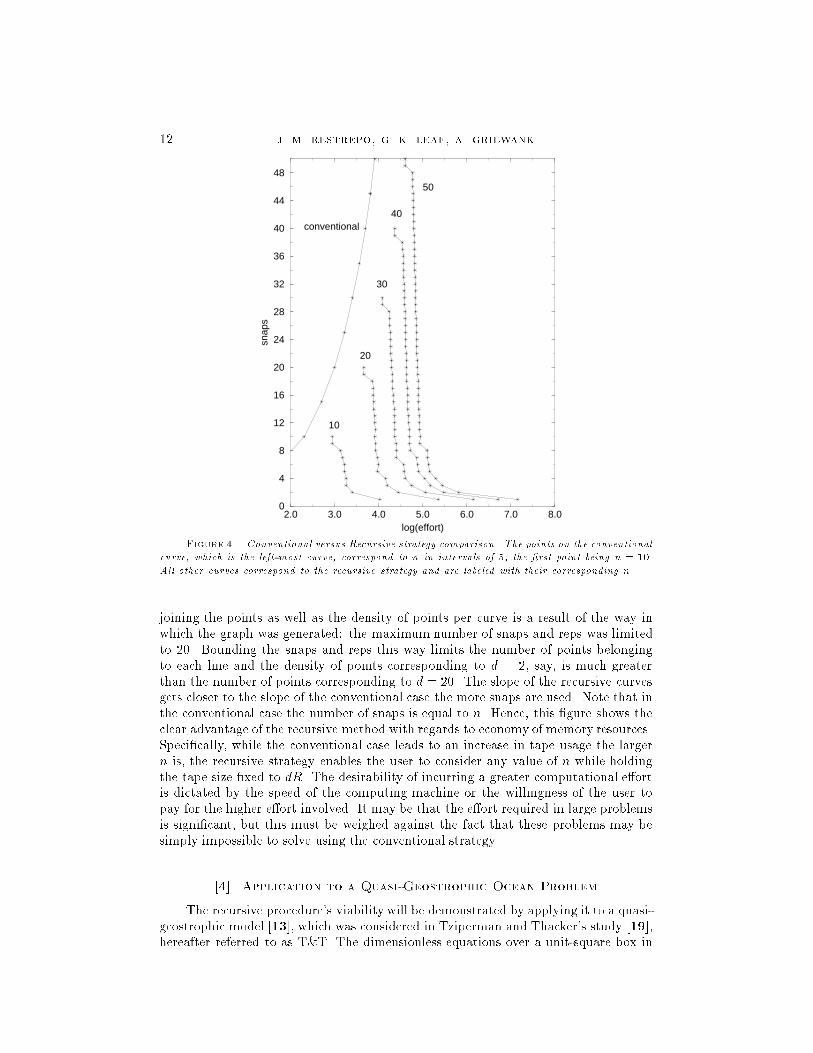
Figure 3. Conventional versus Recursive strategy comparison. The added e�ort due toincreased reps r. From left to right, the conventional case, then r = 1, r = 2, r = 3. The straightcurve corresponds to r = d.is, in e�ect, the limit of snaps d equal to n in the recursive strategy. As can besurmized, the curves re ect the previously mentioned characteristic of the recursivestrategy, namely, that the e�ort increases for the recursive method when fewer snapsare used. Hence, in practice, the user would want to maximize the number of snaps inthe calculation rather than the number of reps. Figure 4 illustrates in greater detailthe memory and computational e�ort dependence on the number of snaps and reps. Inthis �gure it is possible to gauge the relative additional e�ort required by the recursivestrategy over the conventional procedure for a given n. For example, for n = 50 theconventional strategy requires 50 snaps and a logarithm of the e�ort of 3:9, whereasthe recursive strategy for the same n requires as few as 11 snaps with an e�ort ofabout 4:8. As a result, there is an order of magnitude increase in the wall clock time,a very reasonable price to pay for the signi�cant savings in terms of tape memory. Acomparison of Figure 4 and Figure 3 bears this conclusion. In Figure 4 the abruptchanges in the curves for the recursive strategy are a result of changing the value of therep count. The jumping points correspond to places where n = n(d; r). Also noticethat the computational e�ort of the recursive strategy is close but not equal to theconventional case when the number of snaps equals n. This is because in the recursivestrategy every adjoint step is preceeded by a single forward step. Thus, the methodwill accrue an extra n operations in the computational e�ort over the conventionalcounterpart.Figure 5 shows a comparison of the conventional strategy (the left-most curve)with the recursive strategy with regards to the e�ort. The �nite extent of the lines

12 j. m. restrepo, g. k. leaf, a. griewank2.0 3.0 4.0 5.0 6.0 7.0 8.0

log(effort)

0

4

8

12

16

20

24

28

32

36

40

44

48

snap

s

conventional

10

20

30

40

50

Figure 4. Conventional versus Recursive strategy comparison. The points on the conventionalcurve, which is the left-most curve, correspond to n in intervals of 5, the �rst point being n = 10.All other curves correspond to the recursive strategy and are labeled with their corresponding n.joining the points as well as the density of points per curve is a result of the way inwhich the graph was generated: the maximum number of snaps and reps was limitedto 20. Bounding the snaps and reps this way limits the number of points belongingto each line and the density of points corresponding to d = 2, say, is much greaterthan the number of points corresponding to d = 20. The slope of the recursive curvesgets closer to the slope of the conventional case the more snaps are used. Note that inthe conventional case the number of snaps is equal to n. Hence, this �gure shows theclear advantage of the recursive method with regards to economy of memory resources.Speci�cally, while the conventional case leads to an increase in tape usage the largern is, the recursive strategy enables the user to consider any value of n while holdingthe tape size �xed to dR. The desirability of incurring a greater computational e�ortis dictated by the speed of the computing machine or the willingness of the user topay for the higher e�ort involved. It may be that the e�ort required in large problemsis signi�cant, but this must be weighed against the fact that these problems may besimply impossible to solve using the conventional strategy.[4]. Application to a Quasi-Geostrophic Ocean ProblemThe recursive procedure's viability will be demonstrated by applying it to a quasi-geostrophic model [13], which was considered in Tziperman and Thacker's study [19],hereafter referred to as T&T. The dimensionless equations over a unit-square box in

circumventing storage limitations 13Table 1Schedule details for several sets of snaps d, reps r, and steps n.steps snaps reps e�ort reverses reads writes252 5 5 1302 252 251 126126 5 4 546 126 125 70126 4 5 630 126 125 5670 4 4 294 70 69 3556 5 3 196 56 55 3556 3 5 266 56 55 2135 4 3 119 35 34 2035 3 4 140 35 34 1521 5 2 56 21 20 1521 2 5 91 21 20 620 3 3 65 20 19 1015 4 2 39 15 14 1015 2 4 55 15 14 510 3 2 25 10 9 610 2 3 30 10 9 46 5 1 11 6 5 56 2 2 14 6 5 36 1 5 21 6 5 15 4 1 9 5 4 45 1 4 15 5 4 14 3 1 7 4 3 34 1 3 10 4 3 13 2 1 5 3 2 23 1 2 6 3 2 12 1 1 3 2 1 1x and y are �t + x +RoJ( ; �) = ��b� + �h�� + curl�� = � ;(4.1)where (x; y; t) and �(x; y; t) are the streamfunction and the vorticity, � (x; y) is thewind stress, J(�; �) is the Jacobian of its arguments, � is the Laplacian operator, andthe x and t subscripts connote partial derivatives. The dimensionless real parametersRo, �b, and �h are the Rossby number, the bottom friction factor, and the horizontalfriction factor, respectively. The state variables evolve in time t and are subject tono- ux and no-stress boundary conditions at the edges of the box.The equations were discretized using multigrid �nite-di�erence techniques. Inwhat follows it will be understood that the state variables are de�ned only on theuniformly discretized grid in x and y. For the sake of clarity explicit mention that thesequantities are discretized in space will be omitted. The model (4.1) will be integratedforward in time taking equally-spaced time intervals, hence �tl = �t. The recordingand reading of the history will coincide with the integration time steps. Hence �t = �t.On a discrete time grid ti = i�t, according to T&T, the state variables �i and i evolveto a steady state e� and e . In [19], the authors de�ned an assimilation problem asfollows. The observational data was taken to be the steady-state vorticity e�, which is

14 j. m. restrepo, g. k. leaf, a. griewank0.0 2.0 4.0 6.0 8.0 10.0 12.0

log(effort)

0.0

2.0

4.0

6.0

8.0

10.0

12.0

log(

n)

conventional

d=2

d=3

d=10

d=20

Figure 5. Comparison of the conventional and recursive strategy. The memory requirementof the conventional case is n. The recursive curves are labeled according to the number of snaps dused. Natural logarithms are used.independent of time. The vector of control variables is comprised of the forcing termcurl� , the initial vorticity �0, and the parameters �b and �h. The observations e� aredetermined from a particular (�xed) choice of friction factors e�b and e�h, initial vorticity�0, and forcing curle� . The system was then integrated forward in time until a steadystate was reached, at which point the observations were written. For purposes of thisarti�cial assimilation problem, the state set values which produced the observationsare then \forgotten." The task of the assimilation will then be to reconstruct thestate set that generated the observations. To this end, a cost function is chosenthat measures the �t of the model result to the observations. Since the observationsrepresent the steady state, the cost function should measure the departure of themodel from steady state as well as the departure from the observations. In [19] theauthors use the following discrete cost function:Hn(curl�; �0; �b; �h) =XhC(�0 � b�)2 +D(�n � �0)2i ;where the sum indicates a sum over all the discrete values of the variables over theunit box. The �rst term measures the deviation from the observations, while thesecond term in conjunction with the �rst measures the deviation from steady state.The matrices C and D are the inverses of the covariance matrices of the observations.The �nal time step, n, is arbitrary in this problem. It is chosen to be su�ciently largeso that the steady state is reached. A small value of n reduces the computational cost

circumventing storage limitations 15per optimization iteration; however, it increases the number of optimization iterations.Since the number of written histories depends on the number of time steps n, thestorage requirements are reduced when n is small.The goal was to �nd the optimal vector of control variables fcurl�; �0; �b; �hg forwhich Hn is a minimum subject to the constraints of the model equations. A commonstrategy for computing the minimum is to introduce Lagrange multipliers and thecorresponding Lagrange functions for which an unconstrained extremum is sought.A gradient-based iterative algorithm, such as the conjugate gradient method, is thenapplied to this unconstrained problem. For the discrete quasi-geostrophic model, theLagrange function has the formLn = Hn +X nXi=0 �i[�i �� i]+X nXi=1 �i�@�i@t + @ i�1@x + RoJ( i; �i) + �b�i�1 � �h��i�1 � curl�� :The descent algorithm requires the calculation of the gradient of Ln with respectto the state set. The gradient involves the Lagrange multipliers f�i; �ig, which aredetermined from the gradients of Ln with respect to f�i; ig. Equating these gradi-ents to zero generates the adjoint equations for f�i; �ig, which may be symbolicallyexpressed as �t + �x + Ro[J(�;� )��J(�; )] = �b� � �h��+ ;�� = �;(4.2)where is the forcing term arising from the gradients of the cost function with respectto f�i; ig. The discrete adjoint equations are integrated backward in time to generatethe Lagrange multipliers �i used in computing the gradients of the cost function asneeded by the conjugate gradient procedure. Thus, in the conventional approach, eachconjugate gradient iteration requires a forward integration of n steps, which generatesthe value of the cost function, followed by a backward integration of the adjoint equa-tions. This adjoint integration generates the gradients used in the conjugate gradientiteration. Note that the state set is required to e�ect the calculation of the Lagrangemultipliers from the adjoint equations. Thus, in the conventional approach involvingn time steps, n state sets have to be recorded. Since only the state variables are timedependent in this particular problem, we need only to write the state variables �i; iat each time step. The remaining components of the state set need to be written onlyonce during the forward-backward sweep. The observations were synthesized by run-ning the discretized version of (4.1) to steady-state using curl� = � sin(�x) sin(�y),�b = 0:05, �h = 0:0001, and Ro = 0:01.The issue of whether (4.1) has a steady-state solution or the issue concerning theappropriateness of including transients that occur during the spin-up of the model inthe state set in the assimilation procedure is beyond the scope of this study. Our aimis to illustrate the performance characteristics of the recursive algorithm and comparethem to the conventional strategy using an actual code of a non-trivial geophysicalproblem. In T&T's study, n = 1. In their experiment, such a choice is possible sincethe assimilation occurs at just one time level. The role of the integration time lengthin connection to T&T's problem was investigated by Marotzke [9], where he concludedthat in this quasi-geostrophic model, advective phenomena would not adjust quicklyenough. Marotzke suggested that the assimilation be carried out over longer time

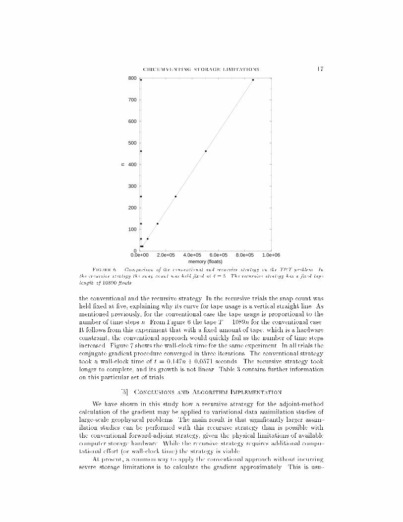
16 j. m. restrepo, g. k. leaf, a. griewankspans. Hence there is some exibility in choosing the integration time, since the onlyrequirement is that it must be longer than n�, where n� is the minimum numberof steps for a steady-state solution. In the general case, assimilations may occur atmultiple time levels, in which case the number of time steps used is determined by theproblem and cannot be arbitrarily chosen.To demonstrate the performance of the recursive forward-backward integrationstrategy for the calculation of the gradient, we compared model runs of this experimentusing the original multigrid Fortran code against a version of the code which wasidentical in all respects to T&T's code, except for a subroutine that generates theschedule and for minor modi�cations to the program to enable us to implement theschedule. As a �rst step, we veri�ed that our program yielded identical results to theconventional code. The wall-clock time was negligibly higher for the recursive programrunning in the conventional mode, re ecting the additional computational expense ofgenerating the schedule and the extra n single forward steps per conjugate gradientstep that are part of the recursive strategy's computational overhead (see Figure 4and comments in Section 3).In the experiments to be reported, the optimality tolerance for the NAG conjugategradient routine was set to 10�3 in all model runs. The square of i � i�1 summedover the box was used to compare against the error tolerance in the conjugate-gradientcalculation. The forward run used to create the observations stepped in time untilthe residual was below 10�7. The multigrid depth was �xed at four levels in allthe experiments. The codes were executed on a Sparc 10/51 running SunOS 4.1.3U1.The Fortran Sun compiler used was Fortran Version 1.4 with optimization ags turnedo�. All runs were performed in double-precision arithmetic. Wall-clock times reportedencompass the solution to the full problem. In all experiments performed, the answersfrom both strategies were identical.To illustrate how the two strategies compare, suppose that for a given resolutionthe T&T problem just \�ts" storage-wise and thus can be solved on a particularmachine using the conventional approach. In order to double the spatial resolution,the conventional strategy would require a sixteenfold increase in tape storage: fourfolddue to the increase in resolution, and fourfold for the increase in the number of timesteps. The doubly resolved experiment no longer could be performed on this particularmachine. However, the problem could be solved by using the recursive approach aslong as the maximum tape length was not exceeded. Suppose that the maximum tapelength on this hypothetical machine is 100000 oats. The tape storage requirementof the singly resolved T&T problem with n = 56 and a 32 � 32 spatial grid withfour re�nement levels is 60984 oats. Table 2 provides the results of a couple ofruns using the recursive strategy for the doubly-resolved problem. Supposing thatthe conventional procedure could be carried out, for n = 224, the tape length for thedoubly-resolved problem would have been 946400 oats, clearly, more storage than themachine is equipped to handle, and it would have taken 153:56 seconds to execute. Thetable demonstrates that the doubly-resolved problem can be succesfully carried outin approximately twice as much time as it would have taken to run the conventionalprocedure assuming that it could be possible to compute conventionally in the �rstplace. Hence, the problem could be done using the recursive strategy in twice theamount of time as the conventional strategy but with twenty times less tape storage.A di�erent situation in which tape length is a limiting factor in assimilationstudies arises when the integration times are very long, causing the state set historystored on tape to be extremely large. Figure 6 shows a comparison of tape usage for

circumventing storage limitations 170.0e+00 2.0e+05 4.0e+05 6.0e+05 8.0e+05 1.0e+06

memory (floats)

0

100

200

300

400

500

600

700

800

n

Figure 6. Comparison of the conventional and recursive strategy on the T&T problem. Inthe recursive strategy the snap count was held �xed at d = 5. The recursive strategy has a �xed tapelength of 10890 oats.the conventional and the recursive strategy. In the recursive trials the snap count washeld �xed at �ve, explaining why its curve for tape usage is a vertical straight line. Asmentioned previously, for the conventional case the tape usage is proportional to thenumber of time steps n. From Figure 6 the tape T = 1089n for the conventional case.It follows from this experiment that with a �xed amount of tape, which is a hardwareconstraint, the conventional approach would quickly fail as the number of time stepsincreased. Figure 7 shows the wall-clock time for the same experiment. In all trials theconjugate gradient procedure converged in three iterations. The conventional strategytook a wall-clock time of t = 0:147n + 0:0571 seconds. The recursive strategy tooklonger to complete, and its growth is not linear. Table 3 contains further informationon this particular set of trials.[5]. Conclusions and Algorithm ImplementationWe have shown in this study how a recursive strategy for the adjoint-methodcalculation of the gradient may be applied to variational data assimilation studies oflarge-scale geophysical problems. The main result is that signi�cantly larger assim-ilation studies can be performed with this recursive strategy than is possible withthe conventional forward-adjoint strategy, given the physical limitations of availablecomputer storage hardware. While the recursive strategy requires additional compu-tational e�ort (or wall-clock time) the strategy is viable.At present, a common way to apply the conventional approach without incurringsevere storage limitations is to calculate the gradient approximately. This is usu-

18 j. m. restrepo, g. k. leaf, a. griewank0.0 50.0 100.0 150.0 200.0 250.0 300.0 350.0 400.0

time (seconds)

0

100

200

300

400

500

600

700

800

n

Figure 7. Comparison of the conventional (left) and recursive (right) strategy for the T&Tproblem. In the recursive strategy the snap count was held �xed at d = 5.Table 2Wall-clock time and tape length for the recursive andconventional approaches in the T&T problem for a doubling of resolution. n = 224.Strategy Time (sec) Tape ( oats) Snaps Repsrecursive 356.94 42250 10 3recursive 315.92 84500 20 2conventional 153.56 946400Table 3Ratio of the wall-clock time for the recursive (withd = 5)to the conventional approach versus n and number of reps for the T&T problem.n Time Ratio Reps21 1.7665 256 2.0687 3126 2.3139 4252 2.5274 5462 2.8306 6792 3.0425 7ally accomplished by recording data far less frequently than is really required, or bytaking advantage of the speci�c circumstances of the problem to eliminate state setcomponents that are known to have little in uence on the gradient and can thus beignored. Obviously, these are tactics are only satisfactory in very speci�c applications.

circumventing storage limitations 19The recursive strategy presented in this study, on the other hand, yields the gradientwithout sacri�cing accuracy in all sets of circumstances and without incurring storagelimitations.In practice, the strategy is best used by chosing the maximum number of snapsthat the particular computer hardware can manage, thus minimizing the number ofreps. This achieves the gradient computations in the shortest wall-clock time. Whenthe number of snaps and reps (i.e., the number of storage units measured in R, andthe number of additional unrecorded forward runs) is equal, these are both boundedby log4 n, where n is the number of time steps in the evolution equation.Insofar as computer program design, the best strategy for large-scale problems isto construct programs that are as compute-intensive as possible and the least memory-intensive. This yields the greatest variation in the computational e�ort for any givenchoice of snaps and reps. This is especially true in parallelized programs becausethe computational e�ort will drop as more processors are used, whereas the storagerequirements remain �xed independent of the number of processors.The implementation of the recursive strategy requires minimal modi�cation ofconventional codes that compute forward and adjoint problems. The requirementsare that four modules be provided: (1) a forward module that runs without writingthe state set between a speci�ed starting and an ending time step; (2) a module thatcomputes a single unrecorded forward and a single adjoint step, given a speci�c timestep; (3) a module that writes to tape the state set at the current time step; and (4)a module that retrieves from tape the last recorded state set. An additional module,which is to be considered the driver, runs the above-mentioned modules according tothe recursive schedule. The driver requires as input the total number of time stepsn, the number of snaps d, where it is understood that the time steps are assimilationtime steps rather than physical time steps and that these steps are not required to beof equal length. The number of reps r is determined once n and d are �xed.One approach in the implementation of the schedule driver is to have the schedulecomputed only once at the top of the program. The schedule instructions are savedin integer arrays, which are then called in sequence to drive the four modules. Thebene�t of precomputing the schedule is not warranted in some applications, sincethe schedule module increases insigni�cantly the overall computational e�ort. Thepreferred alternative is to use the schedule driver to control the above-mentionedmodules, thus not wasting register memory for the schedule arrays needed in the �rstapproach that could otherwise be used in the adjoint problem. An estimate of theadditional memory for the integer schedule arrays of the �rst approach is as follows:a \schedule array" with the instruction directives of size 2rn is required, plus oneor two arrays of similar size that direct the writing and reading of snaps from tape.The total register overhead is then on the order of 4rn integers. The user's particularapplication will clearly dictate which alternative works best.This schedule driver is available via anonymous ftp from ftp.math.ucla.edu.The �le is called /pub/restrepo/treeverse.f. The schedule driver is also availablefrom the Word-Wide-Web http://www.math.ucla.edu/�restrepo.References1. P. COURTIER, J. N. TH�EPAULT and A. HOLLINGSWORTH, A strategy for opera-tional implementation of 4D-VAR using an incremental approach, Preprint, 1993.

20 j. m. restrepo, g. k. leaf, a. griewank2. J. C. DERBER, Variational four dimensional analysis using quasi-geostrophicconstraints, Mon. Wea. Rev. 115 (1987), 998{1008.3. F. X. L. DIMET and O. TALAGRAND, Variational algorithms for analysis andassimilation of metereological observations, Tellus, Series A 38 (1986), 97{110.4. B. F. FARRELL and A. M. MOORE, An adjoint method for obtaining the mostrapidly growing perturbation to oceanic ows, Journal of Physical Oceanography 22(1992), 338{349.5. M. GHIL, Metereological data assimilation for oceanographers. Part I: Descrip-tion and theoretical framework, Dynamics of Atmospheres and Oceans 14 (1989), 171{218.6. A. GRIEWANK, On Automatic Di�erentiation, in Mathematical Programming,M. Iri and K. Tanabe, eds., Kluwer Academic Publishers, Tokyo, 1989, 83{107.7. , Achieving Logarithmic Growth in Temporal and Spatial Complexityin Reverse Automatic Di�erentiation, Optimization Methods and Software 1 (1992),35{54.8. L. M. HOCKING, Optimal Control, An Introduction to the Theory with Appli-cations, Clarendon Press, London, 1991.9. J. MAROTZKE, The role of integration time in determining a steady state throughdata assimilation, Journal of Physical Oceanography 22 (1992), 1556{1567.10. J. MAROTZKE and C. WUNSCH, Finding the steady state of a general circulationmodel through data assimilation: application to the North Atlantic Ocean, Journal ofGeophysical Research 98, C11, 20149{20167.11. NATIONAL ACADEMY PRESS, Four-Dimensional Model Assimilation of Data, AStrategy for the Earth System Sciences, National Research Council, 1991.12. I. M. NAVON, X. ZOU, J. DERBER and J. SELA, Variational data assimilationwith an adiabatic version of the NMC spectral model, Monthly Weather Review 120(1992), 1433{1446.13. J. PEDLOSKY, Geophysical Fluid Dynamics, Springer-Verlag, New York, 1979.14. J. SCHROTER and C. WUNSCH, Solution of nonlinear �nite di�erence oceanmodels by optimization methods with sensitivity and observational strategy analysis,Journal of Physical Oceanography 16 (1986), 1855{1874.15. J. SHEINBAUM and D. L. T. ANDERSON, Variational Assimilation of XBT Data,Journal of Physical Oceanography 20 (1990), 672{688.16. O. TALAGRAND and P. COURTIER, Variational assimilation of meteorologicalobservations with the adjoint vorticity equation, Part I, Theory, Quart. J. Roy. Met.Soc. 113 (1987), 1311{1328.17. W. C. THACKER, Oceanographic inverse problems, Physica D (1992).18. W. C. THACKER and R. B. LONG, Fitting Dynamics to Data, Journal of Geo-physical Research 93, C2, 1227{1240.19. E. TZIPERMAN and W. C. THACKER, An optimal control-adjoint equationsapproach to studying the oceanic general circulation, J. Phys. Ocean. 19 (1989), 1471{1485.20. X. ZOU, I. M. NAVON, A. BARCILON, J. WHITTAKER and D. CACUCI,An adjointsensitivity study of blocking in a two-layer isentropic model, Monthly Weather Review121 (1993), 2833{2857.