Chem. Biochem. Eng. Q. Support Vector Machine-based Soft ...

S. Herceg et al., Support Vector Machine-based Soft Sensors…, Chem. Biochem. Eng. Q., 34 (4) 243–255 (2020) 243

Support Vector Machine-based Soft Sensors in the Isomerisation Process+

S. Herceg,* Ý. Ujević Andrijić, and N. BolfFaculty of Chemical Engineering and Technology, University of Zagreb, Department of Measurements and Process Control, Savska c. 16/5a, 10 000 Zagreb, Croatia

This paper presents the development of soft sensor empirical models using support vector machine (SVM) for the continual assessment of 2,3-dimethylbutane and 2-methyl-pentane mole percentage as important product quality indicators in the refinery isomeri-sation process. During the model development, critical steps were taken, including selec-tion and pre-processing of the industrial process data, which are broadly discussed in this paper. The SVM model results were compared with dynamic linear output error model and nonlinear Hammerstein-Wiener model. Evaluation of the developed models on inde-pendent data sets showed their reliability in the assessment of the component contents. The soft sensors are to be embedded into the process control system, and serve primarily as a replacement during the process analysers’ failure and service periods.

Key words: support vector machine, soft sensor, isomerisation process, process analyser

Introduction

Process analysers, used for measurement of key process variables, are often weak links in refin-ery plants. Their long analysis time, tendency of failure, and high price usually make them impracti-cal and unprofitable. Soft sensors that enable re-al-time prediction of key product properties occur as an alternative to process analysers.

Rarely used as first principle modelling and more often as data-driven mathematical models, soft sensors can well describe dynamics of complex in-dustrial processes1.

This paper presents data-driven soft sensors which have common steps in the development pro-cedure: selection of real process data from plant history database, data pre-processing, determination of a model structure and regressors, model estima-tion and validation2.

The support vector machine is a popular meth-od for soft sensor model development presented by Vapnik3 as part of a general learning theory. The method has attractive features, such as the ability to learn well with only a very small number of free

parameters, robustness, and computational efficiency compared to several other methods4.

The method is widely used for nonlinear sys-tem identification required in the process industry.

The application of SVM has been described in many published papers over the past few years. Meng et al.5 developed data-driven soft sensor based on twin support vector regression for cane sugar crystallisation. Ibrahim et al.6 used SVM and surrogate column models for a novel optimisa-tion-based design of crude oil distillation units. Lv et al.7 proposed SVM-based model for puerarin ex-traction. Shokri et al.8 developed SVM model for the prediction of the content of hydrogen sulphide in the hydrotreatment (HDT) refinery process. Sup-port vector machine is presented in the papers by Xu et al.9 where least squares support vector ma-chine (LS-SVM) is used for gas flow measurements, while Cheng and Liu10 used LS-SVM to propose online soft sensor for product quality monitoring in propylene polymerisation process. Some earlier works should be mentioned, such as the paper by Yan et al.11 where SVM was introduced during soft sensor modelling for light gas oil freezing point as-sessment in the distillation process, as well as the paper by Li et al.12 who developed the model for kerosene dry point assessment based on least squares support vector machine (LS-SVM).

The research and application of soft sensors on an isomerisation process are still rare. Lukec et al.13 proposed application of a software analyser for online

+This paper was presented at the Meeting of Young Chemical Engineers 2020 at the Faculty of Chemical Engineering and Technology, Univer-sity of Zagreb*Corresponding author: Srečko Herceg: [email protected]; [email protected]

This work is licensed under a Creative Commons Attribution 4.0

International License

https://doi.org/10.15255/CABEQ.2020.1825

Original scientific paper Received: May 20, 2020

Accepted: November 29, 2020

S. Herceg et al., Support Vector Machine-based Soft Sensors…243–255

https://doi.org/10.15255/CABEQ.2020.1825

244 S. Herceg et al., Support Vector Machine-based Soft Sensors…, Chem. Biochem. Eng. Q., 34 (4) 243–255 (2020)

estimation of isopentane content in the deisopentan-iser column top product, in the feed treatment sec-tion for the isomerisation process, while Xianghua et al.14 presented the model for para-xylene content estimation at an isomerisation unit reactor outlet.

In our research, development of soft sensor em-pirical models based on SVM for the continual as-sessment of mole percentage of 2,3-dimethylbutane and 2-methylpentane in the product streams of the refinery isomerisation process is presented. These components directly affect the octane number of the isomerate – the product of the isomerisation pro-cess. The model development procedure and the model results are presented and discussed.

Material and methods

In this section, SVM, along with the dynamic output error and Hammerstein-Wiener model struc-ture are briefly explained. A particular part is dedi-cated to the description of the refinery isomerisation process, while soft sensor model development is explained in detail.

SVM model structure

The basic idea of support vector machine can be expressed as shown in Fig. 1. Input space ob-jects, separated with a complex non-linear curve, are mapped (rearranged) into a so-called feature space, where the objects are linearly separable, i.e., an optimal separable curve can be found15.

Mathematically it can be represented by Eq. (1), where the feature space linear regression function is a solution to the nonlinear regression problem: ( ) ( ( ))f b= ⋅Φ +x w x (1)where x is the input vector, w is the load vector, b is a non-variable value, Φ(x) is a “feature” function, and (w · Φ(x)) is the scalar product in the “feature” space. In order to obtain a model, the optimisation problem of so-called structural risk minimisation

principle should be solved. Employing the com-monly used ε-intensive cost function and inserting an adjusting constant C, problem, which is being optimised, from Eq. (1) we obtain:

(2)

2 *

1

1min ( )2

n

i ii

C ξ ξ=

+ +∑w

with the following constraints:

(3)

*

*

( )

( )

, 0; 1,2,...,

i i i

i i i

i i

x b y

y x b

i n

ε ξ

ε ξ

ξ ξ

⋅ + − ≤ +

− ⋅ + ≤ +

≥ =

w

w

where the adjusting constant, C, is a “penalty” fac-tor of the model complexity 2w , while ε is the pa-rameter of the ε-intensive cost function and rep-resents the tube radius located around the function f(x) (Fig. 2)15.

Deviation outside the [ε, -ε] region denotes the forecast error, represented by formulation *

1( )

n

i ii

C ξ ξ=

+∑ , using the slack variables ξ and ξ*.

The points on the surface and outside the ε-tube are called support vectors (SV). The percentage of SVs affects the model accuracy – as the percentage of SVs decreases, a more flattened model is obtained and vice versa15.

The solution of the optimization problem ex-pressed in Eq. (2) is presented by the equation:

(4)

*

1( ) ( ) ( , )

n

ii

f K bα α=

= − +∑x x x

where K(x, xi) is a kernel function, and α, α* are Lagrange multipliers. Radial basis function (RBF) is the most used kernel function, and is defined as:

2( , ) exp( )i iK γ= − −x x x x (5)

where γ is the free parameter of RBF. Kernel func-tion “avoids” cumbersome mathematical operations that take up a lot of computational time15.

F i g . 1 – Basic idea of SVM


Dynamic linear OE and nonlinear HW model structure

Dynamic linear and nonlinear models are con-cisely explained by Ljung16.

OE model is the most complex linear dynamic model usually used for soft sensor model develop-ment. The model predictor is

ˆ ˆ( ) [1 ( )] ( ) ( ) ( )y t q y t q u t nk= − + −F B (6)

where B(q) = B1 + B2 q–1 +…+ Bnb q

–nb+1 is polyno-mial matrix by q–1 dimensions n(y)×n(u), nb is the number of past process inputs, and nk is the input time delay expressed by the number of samples. F(q) = 1 + F1 q

–1 + F2 q–2 +…+ Fnf q

–nf is polynomial matrix by q–1 dimensions n(y) × n(y), nf is the num-ber of past outputs predicted by the model.

The most complex nonlinear dynamic model is HW. It has a block structure described by 3 func-

tions: w(t) = f (u(t)) is a nonlinear function trans-forming input data u(t), x(t) = (B / F) w(t) is a linear transfer function where B and F are polynomials of the OE model, and y (t) = h (x(t)) is a nonlinear function mapping output data x(t) from the linear block to the model output. Nonlinear function could be represented with many nonlinear units, such as wavelet, sigmoid, piecewise-linear, and others.

Process description

The goal of the refinery isomerisation process is to upgrade the octane of light straight-run naph-tha, processing paraffin (mainly pentane and hex-ane) together with hydrogen on a low-temperature, noble-metal, fix-bed catalyst, which is mainly used today. In more detail, the feed paraffin is converted to high-octane iso-structures – normal pentane (nC5) to isopentane (iC5), and normal hexane (nC6) to 2,2 and 2,3-dimethylbutane. Process conditions im-prove isomerisation and reduce unfavourable reac-tions (e.g., hydrocracking), and are featured by me-dium operating pressure, low temperature, and low hydrogen partial pressure17.

According to the process flow diagram (Fig. 3), the dried feed is mixed with make-up hydrogen, and heated before entering the reactor section. After passing the reactors, the isomerised product is stabi-lized in the stabilizer column, where the liquid from the stabilizer bottom passes to gasoline blending, while the stabilizer overhead vapour product flows to a fuel gas system, before being caustic scrubbed with in aim of removing the HCl formed from or-ganic chloride added to the reactor feed to maintain catalyst activity17.

F i g . 2 – Graphical representation of SVM15

F i g . 3 – Straight-through isomerisation process17


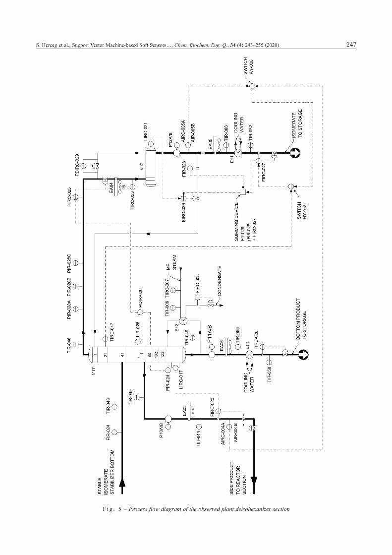
A straight-through isomerization process can be improved by separating the stabilizer bottoms into normal and isoparaffin components by adding a deisohexanizer column (DIH) (Fig. 4).

The DIH column sidecut stream concentrates non-converted n-paraffins and newly-formed low-octane methylpentanes, and returns them to the reactor section. The isomerate is then drawn from the column top, while the heptane fraction is drawn from the column bottom17.

Fig. 5 depicts the process flow diagram of the observed plant deisohexanizer section with the de-isohexanizer column as its part. All process and measuring equipment, as well as control loops, are shown.

Soft sensor model development

2,3-DMB and 2-MP come out as key compo-nents of isomerate – the product of the refinery isomerisation process improved by adding a DIH distillation column. The components affect the oc-tane-number of the product. High-octane 2,3-DMB and low-octane 2-MP mole fractions are measured on-line by process analysers in the DIH sidecut stream and in the DIH overhead, respectively, keep-ing 2,3-DMB in the column top and 2-MP in the side of the column to regulate their molar percent-

age18. The components are also analysed by labora-tory assays once a day.

As the process analysers quite often become unavailable due to failures and have long time de-lays, it was decided to develop soft sensors that would find their applications primarily as the analy-sers’ replacement.

Soft sensor development has a common proce-dure, as follows:– potentially influential variable selection,– data collection and pre-processing,– preliminary research,– model structure and regressor selection, model

estimation, and validation,– model implementation.

Potentially influential variable selection

Based on process studies and consultations with process experts, the potentially influential vari-ables for 2,3-DMB and 2-MP SVM soft sensor mod-el development were selected as shown in Table 1.

Data collection and pre-processing

Experimental data for model development were acquired from the plant history database containing

F i g . 4 – Deisohexanizer column


F i g . 5 – Process flow diagram of the observed plant deisohexanizer section


up to a few years back historical data recorded ev-ery minute.

Data were collected for eight potentially influ-ential variables (Table 1), and for 2,3-DMB and 2-MP content. Special attention was paid to select-ing the data period covering significant process dy-namics. After the data were collected over several periods, lasting from 2–3 weeks to about 2 years, the data were pre-processed, including sample peri-od determination, detection of outliers, and interpo-lation of missing data.

According to process dynamics influential vari-able (further referred to as input variable), the sam-ple period of 3 minutes was evaluated as suitable. Process analyser data (further referred to as output variable) sample period was 30 minutes. The miss-ing data were interpolated using cubic spline inter-polation.

Additional data can be generated using cubic spline or Multivariate adaptive regression spline methods. MARSpline is normally used where there is more than one input variable, as well as when the output variable sample time is long19. Otherwise, the data interpolated using cubic spline have no physical bases, i.e., a relationship between input and output variables is not taken into account. How-ever, due to the fact that refinery processes are quite inertial, this method can be considered sufficiently reliable20.

The common methods for detection of outliers are 3-sigma21, as well as principal component anal-ysis (PCA) and partial least squares (PLS) meth-ods22, which perform only statistical inspection of data and tend to remove peak values that can con-tain useful information about process dynamics. Therefore, the procedure of outlier detection cannot be a fully automated process, and data always should be checked visually. All data collected were visually checked and the amount of outliers detect-ed was negligible.

Preliminary research

Since SVM models are static, it is very import-ant to determine the output variable time delays re-garding the change in the value of each input vari-able.

The output variable time delays were deter-mined for 2,3-DMB and 2-MP content, respectively. For this purpose, an experiment on the observed plant was performed.

In the case of 2,3-DMB, it was observed how a change in one variable caused changes in others. As may be seen in Fig. 5, the V17 reflux flow rate (FIR-028) was reduced slightly, and measured were the time periods until the change in the V17 over-head vapor temperature (TIR-046), in the 21st V17 tray temperature (TIRC-047), and finally in the val-ue of 2,3-DMB content in the V17 side product (de-termined by AIR-004B chromatograph). A relative-ly quick response was noticed. After 2 minutes, the top column temperature (TIR-046) and the tempera-ture on the 21st tray (TIRC-047) started to rise. Af-ter 4 minutes, 2,3-DMB content reacted in the side product – it increased slightly. At once, 2,3-DMB content value time delay in regards to the change in FIR-028 and FIRC-029 input variable, respectively, was 4 minutes. Consequently, it was concluded that, for TIR-046 and TIRC-047 input variable, respec-tively, time delay was 2 minutes. Since TIR-045 in-put variable was installed upstream of the AIR-004B chromatographic analyser, and between them there were only the P10A/B pump and the EA03 air cooler, the time delay was short (0 – 2 minutes). Therefore, time delays were determined exactly for the following variables: TIR-046, TIRC-047, TIR-045, FIR-028 and FIRC-029.

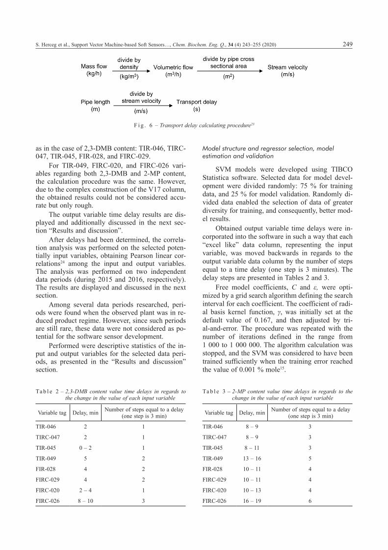
In the case of 2-MP time delays, 2-MP content (determined by the AIR-005B chromatograph) had not changed during the experiment. In order not to affect the process regime, the experiment could not be carried out further and had to be stopped. There-fore, the output variable time delays in this case were determined by a calculation procedure. The main issue was to determine the time until the com-position in the V12 separator had changed. Due to the relatively large separator volume (about 107 m3), change in composition took considerable time. Based on simple hydraulic calculation schematical-ly represented in Fig. 623, using data on the mass flow rate of the V17 top product vapours, density, pipe diameters and lengths between the V17 col-umn, the V12 separator and the AIR-005B chro-matograph, as well as the V12 volume, the time until the composition in the V12 separator had changed was calculated. Taking into account the data obtained by the experiment, 2-MP content val-ue time delays were determined for those variables

Ta b l e 1 – Potentially influential variables18

Variable Tag Unit

V17 overhead vapor temperature TIR-046 °C

21st V17 tray temperature TIRC-047 °C

V17 side product temperature TIR-045 °C

V17 bottom product temperature TIR-049 °C

V17 reflux flow FIR-028 m3 h–1

V17 reflux flow and isomerate flow to storage sum FIRC-029 m3 h–1

V17 side product flow FIRC-020 m3 h–1

V17 bottom product flow FIRC-026 m3 h–1


as in the case of 2,3-DMB content: TIR-046, TIRC-047, TIR-045, FIR-028, and FIRC-029.

For TIR-049, FIRC-020, and FIRC-026 vari-ables regarding both 2,3-DMB and 2-MP content, the calculation procedure was the same. However, due to the complex construction of the V17 column, the obtained results could not be considered accu-rate but only rough.

The output variable time delay results are dis-played and additionally discussed in the next sec-tion “Results and discussion”.

After delays had been determined, the correla-tion analysis was performed on the selected poten-tially input variables, obtaining Pearson linear cor-relations24 among the input and output variables. The analysis was performed on two independent data periods (during 2015 and 2016, respectively). The results are displayed and discussed in the next section.

Among several data periods researched, peri-ods were found when the observed plant was in re-duced product regime. However, since such periods are still rare, these data were not considered as po-tential for the software sensor development.

Performed were descriptive statistics of the in-put and output variables for the selected data peri-ods, as presented in the “Results and discussion” section.

Model structure and regressor selection, model estimation and validation

SVM models were developed using TIBCO Statistica software. Selected data for model devel-opment were divided randomly: 75 % for training data, and 25 % for model validation. Randomly di-vided data enabled the selection of data of greater diversity for training, and consequently, better mod-el results.

Obtained output variable time delays were in-corporated into the software in such a way that each “excel like” data column, representing the input variable, was moved backwards in regards to the output variable data column by the number of steps equal to a time delay (one step is 3 minutes). The delay steps are presented in Tables 2 and 3.

Free model coefficients, C and ε, were opti-mized by a grid search algorithm defining the search interval for each coefficient. The coefficient of radi-al basis kernel function, γ, was initially set at the default value of 0.167, and then adjusted by tri-al-and-error. The procedure was repeated with the number of iterations defined in the range from 1 000 to 1 000 000. The algorithm calculation was stopped, and the SVM was considered to have been trained sufficiently when the training error reached the value of 0.001 % mole15.

Ta b l e 2 – 2,3-DMB content value time delays in regards to the change in the value of each input variable

Variable tag Delay, min Number of steps equal to a delay (one step is 3 min)

TIR-046 2 1

TIRC-047 2 1

TIR-045 0 – 2 1

TIR-049 5 2

FIR-028 4 2

FIRC-029 4 2

FIRC-020 2 – 4 1

FIRC-026 8 – 10 3

Ta b l e 3 – 2-MP content value time delays in regards to the change in the value of each input variable

Variable tag Delay, min Number of steps equal to a delay (one step is 3 min)

TIR-046 8 – 9 3

TIRC-047 8 – 9 3

TIR-045 8 – 11 3

TIR-049 13 – 16 5

FIR-028 10 – 11 4

FIRC-029 10 – 11 4

FIRC-020 10 – 13 4

FIRC-026 16 – 19 6

F i g . 6 – Transport delay calculating procedure23


Developed models were validated based on FIT values, final prediction error (FPE), root mean square error (RMSE), and mean absolute error (MAE).

Model implementation

Implementation of the model to the refinery isomerisation process is underway. The goal is to implement the developed models into the module for advanced process control in plant DCS. The new variable labels for 2,3-DMB and 2-MP content predicted by the model, will be created and stored in the process history database.

Results and discussion

In this section, the results obtained from data collection and pre-processing, preliminary research – including calculation of input variables time de-lays, performance of the correlation analysis and descriptive statistics, as well as the developed 2,3-DMB and 2-MP content SVM model results com-pared with dynamic linear OE and nonlinear HW model, are presented and discussed.

Interpolation of missing data

Fig. 7 shows a part of cubic spline interpolated output data compared with the real measurements (stepped curve). Very good interpolation of missing data can be observed.

Determining time delays

From Table 2 it can be seen that the time delays are relatively small. AIRC-004A chromatographic analyser on V17 sidecut product line was installed with no upstream accumulated liquid vessel, e.g., a separator, etc. (Fig. 5), that can consequently slow down a mass transfer.

In the case of 2-MP content, the time delays are larger than in the case of 2,3-DMB. This is mainly due to the aforementioned V12 separator, i.e., AIR-005B chromatograph installed downstream of it.

Correlation analysis

Tables 4 and 5 show Pearson’s linear correlation coefficients between the input and output variables within 2015 and 2016 data period, respectively.

Observing the tables, it can be concluded that most of the inputs had significant impact on the out-puts. However, from Table 4 it can be seen that, for all four outputs, the potential input variable FIRC-020 (V17 side product flow) had low correlations, and could be excluded as the model input. Also, for data according to Table 5, the potential inputs FIRC-020 and FIRC-026 (V17 bottom product flow) could be excluded.

The time delays were not taken into account.

Final input variables and model determination periods

Earlier research18 on dynamic polynomial mod-els has shown that much better results had been ob-tained for 2,3-DMB content models during 2015 data period, while in the case of 2-MP, the better results were during 2016. Due to the direct compar-ison of SVM model results with the results of the dynamic polynomial, the development of the pro-posed SVM models was based on the same corre-sponding periods. In the case of 2,3-DMB content SVM model, the range was from November 27 to December 11, 2015, comprising 6 667 measured data, while in the case of 2-MP model, the range was from January 1 to January 21, 2016, compris-ing 10 078 measured data, for each of the input variables and the outputs.

F i g . 7 – Cubic spline interpolated output data and the real analyser output


The final number of the input variables for the development of the SVM models based on the cor-relation coefficient results given in Tables 4 and 5 is given in Tables 6 and 7.

Descriptive statistics

Tables 8 and 9 show the descriptive statistics of the input and output variables within 2015 and 2016 data period, respectively.

Ta b l e 4 – Correlation coefficient results within 2015 data period

TIR 046 TIRC 047 TIR 045 TIR 049 FIR 028 FIRC 029 FIRC 020 FIRC 026 AIR 004B AIR 005B

TIR-046 1.00 0.90 0.71 –0.50 –0.88 –0.33 –0.10 0.36 –0.88 0.93

TIRC-047 1.00 0.65 –0.50 –0.81 –0.23 –0.17 0.26 –0.87 0.84

TIR-045 1.00 –0.39 –0.63 –0.22 –0.20 0.27 –0.62 0.57

TIR-049 1.00 0.38 0.17 0.22 –0.19 0.30 –0.36

FIR-028 1.00 0.43 0.05 –0.24 0.83 –0.83

FIRC-029 1.00 –0.09 –0.18 0.36 –0.32

FIRC-020 1.00 –0.06 0.10 –0.04

FIRC-026 1.00 –0.35 0.42

AIR-004B 1.00 –0.92

AIR-005B 1.00

Ta b l e 5 – Correlation coefficient results within 2016 data period

TIR 046 TIRC 047 TIR 045 TIR 049 FIR 028 FIRC 029 FIRC 020 FIRC 026 AIR 004B AIR 005B

TIR-046 1.00 0.94 0.72 –0.59 –0.68 –0.31 –0.24 –0.22 –0.70 0.82

TIRC-047 1.00 0.73 –0.55 –0.74 –0.28 –0.21 –0.24 –0.75 0.85

TIR-045 1.00 –0.20 –0.33 –0.15 –0.10 –0.17 –0.43 0.45

TIR-049 1.00 0.42 0.11 0.20 0.47 0.29 –0.45

FIR-028 1.00 0.49 0.25 0.24 0.68 –0.78

FIRC-029 1.00 0.23 0.08 0.44 –0.37

FIRC-020 1.00 0.18 0.26 –0.20

FIRC-026 1.00 0.13 –0.08

AIR-004B 1.00 –0.88

AIR-005B 1.00

Ta b l e 6 – Input variables for the development of 2,3-DMB content SVM model

No. Variable Tag Unit

1 V17 overhead vapor temperature TIR-046 °C

2 21st V17 tray temperature TIRC-047 °C

3 V17 side product temperature TIR-045 °C

4 V17 bottom product temperature TIR-049 °C

5 V17 reflux flow FIR-028 m3 h–1

6 V17 reflux flow and isomerate flow to storage sum

FIRC-029 m3 h–1

7 V17 bottom product flow FIRC-026 m3 h–1

Ta b l e 7 – Input variables for the development of 2-MP con-tent SVM model

No. Variable Tag Unit

1 V17 overhead vapor temperature TIR-046 °C

2 21st V17 tray temperature TIRC-047 °C

3 V17 side product temperature TIR-045 °C

4 V17 bottom product temperature TIR-049 °C

5 V17 reflux flow FIR-028 m3 h–1

6 V17 reflux flow and isomerate flow to storage sum

FIRC-029 m3 h–1


Laboratory analyses

Figs. 8 and 9 show comparison between the on-line chromatographic analysers data (2,3-DMB, 2-MP contents) and the laboratory assays within 2015 and 2016 data period, respectively.

From the plots, a good correlation between measured and laboratory data can be observed, which proves the accuracy of the on-line chromato-graphic analysers, i.e., validity of the selected data periods.

Model evaluation results

Based on statistical criteria, Tables 10 and 11 show validation of SVM as well as OE and HW models on validation data set for estimating the content of 2,3-DMB and 2-MP in the isomerisation process DIH column side and top product, respec-tively.

As may be seen from Table 10, 2,3-DMB con-tent SVM model shows superior results compared to both dynamic polynomial OE and HW model, respectively, with only 3 model free coefficients (C, ε and γ).

Table 11 shows that the dynamic models are better; however, with dozens of model free coeffi-cients.

The FIT values, as well as the values of FPE, RMSE, and MAE of the SVM models, indicate sat-

isfactory assessment meaning that the process dy-namics were well described.

It is easy to conclude that the SVM models are better for implementation than dynamic polynomial linear or nonlinear models, which also contributes to the robustness of the SVM models.

Ta b l e 8 – Descriptive statistics within 2015 data period15

Variable Samples Mean Median Min Max Variance Std. dev.

TIR-046 6667 75.43 75.72 72.54 77.57 1.083 1.041

TIRC-047 6667 87.29 87.65 82.55 88.40 1.072 1.035

TIR-045 6667 97.23 97.26 96.19 98.19 0.072 0.268

TIR-049 6667 121.7 121.8 117.4 125.0 1.078 1.038

FIR-028 6667 378.2 377.4 360.8 397.5 38.22 6.182

FIRC-029 6667 426.2 426.5 404.7 448.9 29.69 5.448

FIRC-026 6667 5.534 5.497 2.966 11.00 1.826 1.351

AIR-004B 6667 7.417 7.278 5.871 10.12 0.605 0.778

Ta b l e 9 – Descriptive statistics within 2016 data period15

Variable Samples Mean Median Min Max Variance Std. dev.

TIR-046 10078 75.93 75.99 73.44 77.89 0.804 0.897

TIRC-047 10078 87.67 87.76 86.26 88.65 0.175 0.418

TIR-045 10078 97.15 97.16 96.21 97.89 0.060 0.245

TIR-049 10078 122.7 122.8 119.6 125.3 1.004 1.002

FIR-028 10078 372.4 372.2 357.1 386.7 36.67 6.056

FIRC-029 10078 422.3 422.6 404.7 439.0 18.19 4.265

AIR-005B 10078 11.05 11.74 4.605 16.91 8.788 2.965

Ta b l e 1 0 – 2,3-DMB content model evaluation

SVM OE18 HW18

FIT (%) 84.67 72.62 73.76

FPE 0.014 0.035 0.102

RMSE (% mole) 0.118 0.213 0.200

MAE (% mole) 0.077 0.156 0.149

Model free coefficient 3 85 156

Ta b l e 11 – 2-MP content model evaluation

SVM OE18 HW18

FIT (%) 82.98 88.02 88.91

FPE 0.249 0.086 0.182

RMSE (% mole) 0.499 0.270 0.260

MAE (% mole) 0.317 0.201 0.196

Model free coefficient 3 87 190


F i g . 8 – Comparison between 2,3-DMB content output variable measured by the on-line chromatographic analyser and the laboratory analysis within 2015 data period

F i g . 9 – Comparison between 2-MP content output variable measured by the on-line chromatographic analyser and the laboratory analysis within 2016 data period

Graphical representation in Figs. 10 and 11 de-picts the comparison between measured data and 2,3-DMB/2-MP content model data, respectively. Very good correspondence between the measured data and model outputs may be observed.

Table 12 shows the comparison between 2,3-DMB and 2-MP SVM content models. 2-MP SVM content model is somewhat more complex than 2,3-DMB – a larger number of SVs was required to achieve an accurate model.

Overall, the obtained results confirm SVM method to be suitable for nonlinear system identifi-cation in chemical plants.

Conclusion

Soft sensor models based on SVM for continu-al assessment of the mole percentage of 2,3-DMB and 2-MP, as the key components in products of the refinery isomerisation process, improved by adding a deisohexanizer, were developed. The models de-scribe the process dynamics very well, and are therefore suitable for implementation within the isomerisation process plant distributed control sys-tem (DCS). Due to its robustness, it is expected that the method will be an alternative to expensive pro-cess analysers.

Ta b l e 1 2 – Comparison between 2,3-DMB and 2-MP SVM models

ModelOptimized coefficients Kernel

functionNumber of SVsC ε γ

2,3-DMB 15 0.001 20 RBF 4748

2-MP 1 0.01 50 RBF 6042


The development and application of soft sen-sors are desirable and often necessary in modern process industry. The requirements for continuous improvements, especially in product quality and minimization of energy consumption, urge in-creased application of soft sensors.

ACKNOWLEDGEMENTS

The authors would like to thank the personnel of “JSC Naftan” refinery, Novopolotsk, the Repub-lic of Belarus, for their help throughout this project.

L i s t o f s y m b o l s a n d a b b r e v i a t i o n s

2,3-DMB – 2,3-dimethylbutane2-MP – 2-methylpentaneb – constantB(q), B1, B2, Bnb – polynomial matrixC – adjusting constantDCS – distributed control system

DIH – deisohexanizerf(x) – regression functionF(q), F1, F2, Fnf – polynomial matrixFIT – fitting coefficientFPE – final prediction errorh(x(t)) – output nonlinearity functionHDT – hydrotreatmentHW – Hammerstein-WienerOE – output errori – numeratoriC5 – isopentaneK(x, xi) – kernel functionLS-SVM – least squares support vector

machineMAE – mean absolute errorMARSpline – multivariate adaptive regression splinen – number of datanb – number of past process inputsnf – number of past model predicted

outputsnk – input time delay expressed by the

number of samples

F i g . 11 – Comparison between measured data and 2-MP content SVM model results

F i g . 1 0 – Comparison between measured data and 2,3-DMB content SVM model results


nC5 – normal pentanenC6 – normal hexanePCA – principle component analysisPLS – partial least squaresq, q–1, q–nb+1, q–nf – time shift operatorRBF – radial basis functionRMSE – root mean square errorSV – support vectorsSVM – support vector machinest – timeu(t) – input data functionw(t) – nonlinear functionw – load vectorx(t) – linear transfer functionx, xi – vector of input datax, xi – input data valuey, yi – output data valueŷ(t) – model output functionα, α* – Lagrange multipliersγ – parameter of radial basis functionε – parameter of ε-intensive cost functionξ, ξ*, ξi, ξi

* – slack variablesΦ(x) – feature function

R e f e r e n c e s

1. Kadlec, P., Gabrys, B., Strandt, S., Data-driven soft sensors in the process industry, Comput. Chem. Eng. 33 (2009) 795.doi: https://doi.org/10.1016/j.compchemeng.2008.12.012

2. Fortuna, L., Graziani, S., Rizzo, A., Xibilia, M. G., Soft Sensors for Monitoring and Control of Industrial Processes (Advances in Industrial Control), Springer-Verlag, London, 2007.doi: https://doi.org/10.1007/978-1-84628-480-9

3. Vapnik, V. N., The nature of statistical learning theory, Springer-Verlag, New York, 1995.doi: https://doi.org/10.1007/978-1-4757-3264-1

4. Steinwart, I., Christmann, A., Support Vector Machines, Springer-Verlag, New York, 2008.doi: https://doi.org/10.1007/978-0-387-77242-4

5. Meng, Y., Lan, Q., Qin, J., Yu, S., Pang, H., Zheng, K., Data-driven soft sensor modeling based on twin support vector regression for cane sugar crystallization, J. Food Eng. 241 (2019) 159.doi: https://doi.org/10.1016/j.jfoodeng.2018.07.035

6. Ibrahim, D., Jobson, M., Li, J., Guillén-Gosálbez, G., Opti-mization-based design of crude oil distillation units using surrogate column models and a support vector machine, Chem. Eng. Res. Des. 134 (2018) 212.doi: https://doi.org/10.1016/j.cherd.2018.03.006

7. Lv, B., Chen, J., Dong, C., Wang, Q., Soft measurement of puerarin extraction based on GA-SVM, 2017 Chinese Automation Congress (CAC), IEEE, Jinan, 2017, pp 5005–5009.doi: https://doi.org/10.1109/CAC.2017.8243667

8. Shokri, S., Sadeghi, M. T., Marvast, M. A., Narasimhan, S., Improvement of the prediction performance of a soft sensor model based on support vector regression for production of ultra-low sulfur diesel, Pet. Sci. 12 (2015) 177.doi: https://doi.org/10.1007/s12182-014-0010-9

9. Xu, W., Fan, Z., Cai, M., Shi, Y., Tong, X., Sun, J., Soft sensing method of LS-SVM using temperature time series for gas flow measurements, Metrol. Meas. Syst. 22 (2015) 383.doi: https://doi.org/10.1515/mms-2015-0028

10. Cheng, Z., Liu, X., Optimal online soft sensor for product quality monitoring in propylene polymerization process, Neurocomputing 149 (2015) 1216.doi: https://doi.org/10.1016/j.neucom.2014.09.006

11. Yan, W., Shao, H., Wang, X., Soft sensing modelling based on support vector machine and Bayesian model selection, Comput. Chem. Eng. 28 (2004) 1489.doi: https://doi.org/10.1016/j.compchemeng.2003.11.004

12. Li, Y., Li, Q., Wang, H., Ma, N., Soft Sensing Based on LS-SVM and Its Application to a Distillation Column, Sixth International Conference on Intelligent Systems Design and Applications, IEEE, Jinan, 2006, pp 177–182.doi: https://doi.org/10.1109/ISDA.2006.246

13. Lukec, I., Lukec, D., Sertić Bionda, K., AdŢamić Z., The possibilities of advancing isomerization process through continuous optimization, Goriva i maziva 46 (2007) 234.

14. Xianghua, C., Ouguan, X., Hongbo, Z., Recursive PLS soft sensor with moving window for online PX concentration estimation in an industrial isomerization unit, Chinese Con-trol and Decision Conference, IEEE, Guilin, 2009, pp 5853–5857.doi: https://doi.org/10.1109/CCDC.2009.5195246

15. Herceg, S., Ujević Andrijić, Ý., Bolf, N., Development of soft sensors for isomerization process based on support vector machine regression and dynamic polynomial mod-els, Chem. Eng. Res. Des. 149 (2019) 95.doi: https://doi.org/10.1016/j.cherd.2019.06.034

16. Ljung, L., System Identification: Theory for the User, 2nd ed., Prentice Hall, New Jersey, 1999.

17. Cusher, N. A., UOP Penex Process, in Meyers, R. A. (Ed.), Handbook of Petroleum Refining Processes, third edition, McGraw-Hill, New York, 2003, pp 9.15–9.27.

18. Herceg, S., Ujević Andrijić, Ý., Bolf, N., Continuous estima-tion of the key components content in the isomerization process products, Chem. Eng. Trans. 69 (2018), 79.doi: https://doi.org/10.3303/CET1869014

19. Mohler, I., Development of soft sensors for refinery advanc ed process control, PhD thesis, Faculty of chemical engineering and technology, University of Zagreb, Zagreb, 2015.

20. Ujević Andrijić, Ý., Softverski senzori za identifikaciju i vođenje nelinearnih procesa, PhD thesis, Faculty of chemi-cal engineering and technology, University of Zagreb, Zagreb, 2012.

21. Pearson, R., K., Outliers in process modeling and identifi-cation, IEEE T. Contr. Syst. T. 10 (2002) 55.doi: https://doi.org/10.1109/87.974338

22. Lin, B., Recke, B., Renaudat, P., Knudsen, J., Jørgensen, S. B., Robust statistics for soft sensor development in cement kiln, 16th Triennial World Congress of International Feder-ation of Automatic Control, Proceeding of 16th IFAC World Congress, Prague, 2005, pp 241–246.doi: https://doi.org/10.3182/20050703-6-CZ-1902.01720

23. Sharmin, R., Sundararaj, U., Shah, S., Griend L. V., Sun Y., Inferential sensor for estimation of polymer quality param-eters: Industrial application of a PLS-based soft sensor for a LDPE plant, Chem. Eng. Sci. 61 (2006) 6372.doi: https://doi.org/10.1016/j.ces.2006.05.046

24. Warne, K., Prasad, G., Rezvani, S., Maguire, L., Statistical and computational intelligence techniques for inferential model development: A comparative evaluation and a novel proposition for fusion, Eng. Appl. Artif. Intell. 17 (2004) 871.doi: https://doi.org/10.1016/j.engappai.2004.08.020

Chem. Biochem. Eng. Q. Support Vector Machine-based Soft ...

Documents