TIME-DEPENDENT PROBLEMS The previous three chapters dealt exclusively with steady- state problems, that is, problems where time did not enter explicitly into the formulation or solution of the problem. The types of problems considered in Chapters 2 and 3, respectively, were one- and two-dimensional elliptic boundary value problems. In this chapter, finite element models for parabolic and hyperbolic equations, such as the one-dimensional transient heat conduction and the one-dimensional scalar wave equation, respectively, will be developed. TIME-DEPENDENT PROBLEMS The wave equation is an important second-order linear partial differential equation for the description of waves – as they occur in physics – such as sound waves, light waves and water waves. It arises in fields like acoustics, electromagnetics, and fluid dynamics. Historically, the problem of a vibrating string such as that of a musical instrument was studied by Jean le Rond d'Alembert, Leonhard Euler, Daniel Bernoulli, and Joseph- Louis Lagrange. TIME-DEPENDENT PROBLEMS A pulse traveling through a string with fixed endpoints as modeled by the wave equation. TIME-DEPENDENT PROBLEMS Spherical waves coming from a point source. TIME-DEPENDENT PROBLEMS Cut-away of spherical wavefronts, with a wavelength of 10 units, propagating from a point source. TIME-DEPENDENT PROBLEMS A solution of the wave equation in two dimensions with a zero-displacement boundary condition along the entire outer edge. CIVL 7/8111 Time-Dependent Problems - 1-D Wave Equation 1/23

Welcome message from author
This document is posted to help you gain knowledge. Please leave a comment to let me know what you think about it! Share it to your friends and learn new things together.
Transcript

TIME-DEPENDENT PROBLEMS
The previous three chapters dealt exclusively with steady-state problems, that is, problems where time did not enter explicitly into the formulation or solution of the problem.
The types of problems considered in Chapters 2 and 3, respectively, were one- and two-dimensional elliptic boundary value problems.
In this chapter, finite element models for parabolic and hyperbolic equations, such as the one-dimensional transient heat conduction and the one-dimensional scalar wave equation, respectively, will be developed.
TIME-DEPENDENT PROBLEMS
The wave equation is an important second-order linear partial differential equation for the description of waves –as they occur in physics – such as sound waves, light waves and water waves.
It arises in fields like acoustics, electromagnetics, and fluid dynamics.
Historically, the problem of a vibrating string such as that of a musical instrument was studied by Jean le Rond d'Alembert, Leonhard Euler, Daniel Bernoulli, and Joseph-Louis Lagrange.
TIME-DEPENDENT PROBLEMS
A pulse traveling through a string with fixed endpoints as modeled by the wave equation.
TIME-DEPENDENT PROBLEMS
Spherical waves coming from a point source.
TIME-DEPENDENT PROBLEMS
Cut-away of spherical wavefronts, with a wavelength of 10 units, propagating from a point source.
TIME-DEPENDENT PROBLEMS
A solution of the wave equation in two dimensions with a zero-displacement boundary condition along the entire outer edge.
CIVL 7/8111 Time-Dependent Problems - 1-D Wave Equation 1/23

TIME-DEPENDENT PROBLEMS
One-Dimensional Wave or Hyperbolic Equations
( , )u x t
L
( )P t
An example of a physical problem whose behavior is described by the classical one-dimensional wave equation is the problem of the longitudinal or axial motion of a straight prismatic elastic bar as indicated below.
dx
( )P t ( )P t dP
TIME-DEPENDENT PROBLEMS
One-Dimensional Wave or Hyperbolic Equations
The basic physical principle governing the motion is Newton's second law which, when applied to a typical differential element as shown above, yields:
dx
( )P t ( )P t dP
2
2x
d uF P P dP Adx
dt
with
duP A AE AE
dx
2
2
u uAE A
x x t
TIME-DEPENDENT PROBLEMS
One-Dimensional Wave or Hyperbolic Equations
The resulting equation:
where A is the area, E is Young's modulus, and is the mass density.
This equation of motion is often referred to as the one-dimensional wave equation in that it is an example of the standard hyperbolic equation that predicts wave propagation in a one-dimensional setting.
2
2
u uAE A
x x t
TIME-DEPENDENT PROBLEMS
One-Dimensional Wave or Hyperbolic Equations
When A and E are constants, the equation is often written as:
2 22
2 2
u uc
x t
with Ec
where c is the speed at which longitudinal waves propagate along the x -axis.
TIME-DEPENDENT PROBLEMS
One-Dimensional Wave or Hyperbolic Equations
Appropriate boundary conditions are:
( , )( ) (0, ) 0
u L tAE P t u t
x
stating that the displacement is zero for all time at x = 0 and that there is a force P(t) applied at x = L.
( ,0)( ) ( , 0) ( )
u xg x u x f x
t
are also prescribed, where f and g represent the initial axial displacement and axial velocity, respectively.
Two initial conditions of the form:
TIME-DEPENDENT PROBLEMS
One-Dimensional Wave or Hyperbolic Equations
Thus a typical initial-boundary value problem associated with the wave equation can be stated as:
2
20 , 0
u uAE A x L t
x x t
Many other physical situations such as the transverse motions of strings and membranes, propagation of sound, and dynamic disturbances in fluids and solids are governed by the wave equation.
(0, ) 0u t
( , )( )
u L tAE P t
x
( , 0) ( )u x f x
( ,0)( )
u xg x
t
CIVL 7/8111 Time-Dependent Problems - 1-D Wave Equation 2/23

TIME-DEPENDENT PROBLEMS
The Galerkin Finite Element Method
As has been indicated numerous times in the preceding material, the first steps in developing a finite element model are discretization and interpolation. These are carried out exactly as before.
1x a 2x 4x · · ·Nx 1Nx b
u
x
nodes
3x
elements
One-Dimensional Wave or Hyperbolic Equations
TIME-DEPENDENT PROBLEMS
The Galerkin Finite Element Method
Consider the one-dimensional wave problem developed in this section.
Discretization. The first step in developing a finite element model is discretization. Nodes for the spatial domain a ≤ x ≤ b are chosen as indicated below, with a = x1
and b = xN+1.
1x a 2x 4x · · ·Nx 1Nx b
u
x
nodes
3x
elements
One-Dimensional Wave or Hyperbolic Equations
TIME-DEPENDENT PROBLEMS
The Galerkin Finite Element Method
Interpolation. Interpolation would again be semidiscrete, of the form:
1
1
( , ) ( ) ( )N
i iu x t u t n x
where the ni(x) are nodally based interpolation functions and can be linear, quadratic, or higher-order if desired.
The elements indicated above are specifically for linear interpolation.
One-Dimensional Wave or Hyperbolic Equations
TIME-DEPENDENT PROBLEMS
The Galerkin Finite Element Method
Elemental formulation. Consider again the initial-boundary value problem developed in the previous section:
One-Dimensional Wave or Hyperbolic Equations
(0, ) 0u t ( , 0) ( )u x f x
( , )( )
u L tAE P t
x
( ,0)
( )u x
g xt
2
20 , 0
u uAE A x L t
x x t
TIME-DEPENDENT PROBLEMS
The Galerkin Finite Element Method
Elemental formulation. The elemental formulation for the wave equation is based on a corresponding weak statement.
The weak form is developed by multiplying the differential equation by a test function v(x) satisfying any essential boundary conditions, with the result then integrated over the spatial region according to:
One-Dimensional Wave or Hyperbolic Equations
2
20
b
a
u uv AE A dx
x x t
TIME-DEPENDENT PROBLEMS
The Galerkin Finite Element Method
Integrating by parts and eliminating the derivative terms from the boundary conditions yields:
2
20
b
a
u uv AE Av dx v L P t
x t
Elemental formulation. The elemental formulation for the diffusion problem is based on a corresponding weak statement.
One-Dimensional Wave or Hyperbolic Equations
which is the required weak statement for the initial-boundary value problem associated with the one-dimensional wave equation.
CIVL 7/8111 Time-Dependent Problems - 1-D Wave Equation 3/23

TIME-DEPENDENT PROBLEMS
The Galerkin Finite Element Method
Elemental formulation. The finite element model is obtained by substituting the approximate solution and v = nk, k = 1, 2, ..., N + 1, successively, into the above expression to obtain:
1
11
( )bN
k i k i kN
a
n AEn n An u dx P t
One-Dimensional Wave or Hyperbolic Equations
TIME-DEPENDENT PROBLEMS
The Galerkin Finite Element Method
Elemental formulation. Which can be written as:
1
1
( ) ( ) ( ) 1,2,..., 1N
ki i ki i kA u t B u t F t k N
b
ki k i
a
A n AEn dx
b
ki k i
a
B n An dx
1 ( )k kNF P t
One-Dimensional Wave or Hyperbolic Equations
TIME-DEPENDENT PROBLEMS
The Galerkin Finite Element Method
Elemental formulation. In matrix notation, the above expression can be written as:
Au Bu F
e e
G GA k B = m
T Tj j
i i
x x
x x
AE dx A dx e ek N N m N N
One-Dimensional Wave or Hyperbolic Equations
0 0 0 .... 0 PF =
TIME-DEPENDENT PROBLEMS
The Galerkin Finite Element Method
Elemental formulation. The original initial-boundary value problem has been converted into the initial value problem:
0 0with (0) (0) Au Bu F u u u u
The vector u0 and ů0, representing the discretized version of the initial conditions f and g, are usually taken to be respectively the vectors consisting of the values of f(x) and g(x) at the nodes, that is:
T
0 2 3(0) (0) ( ) ( ) ... ( ) ( )Nf f x f x f x f L u u
One-Dimensional Wave or Hyperbolic Equations
T
0 2 3(0) (0) ( ) ( ) ... ( ) ( )Ng g x g x g x g L u u
TIME-DEPENDENT PROBLEMS
The Galerkin Finite Element Method
Elemental formulation. Note that the assembly process has taken place implicitly, while carrying out the details of obtaining the governing equations, using the Galerkin method in connection with the weak formulation.
Enforcement of constraints is necessary if either of the boundary conditions is essential, that is, if the dependent variable is prescribed at either boundary point.
One-Dimensional Wave or Hyperbolic Equations
TIME-DEPENDENT PROBLEMS
The Galerkin Finite Element Method
Elemental formulation. The system of equations must be altered to reflect these constraints.
Consider for example, the case where the boundary condition at x = 0 is u(0, t) = u0(t). The first scalar equation of the set of equations would be replaced by the constraint so that there would result:
1 0
21 1 22 2 23 3 21 1 22 2 23 3
31 1 32 2 33 3 31 1 32 2 33 3
( )
0
0
u u t
a u a u a u b u b u b u
a u a u a u b u b u b u
One-Dimensional Wave or Hyperbolic Equations
CIVL 7/8111 Time-Dependent Problems - 1-D Wave Equation 4/23

TIME-DEPENDENT PROBLEMS
The Galerkin Finite Element Method
Elemental formulation. The u1 and terms in the remaining equations are transferred to the right-hand side to yield:
1 0
22 2 23 3 22 2 23 3 21 0 21 0
32 2 33 3 32 2 33 3 31 0 31 0
( )u u t
a u a u b u b u a u b u
a u a u b u b u a u b u
One-Dimensional Wave or Hyperbolic Equations
For a linearly interpolated model the half bandwidth is two, and only the u1 and ü1 in terms in the second equation need be transferred to the right-hand side.
TIME-DEPENDENT PROBLEMS
The Galerkin Finite Element Method
Elemental formulation. The u1 and terms in the remaining equations are transferred to the right-hand side to yield:
1 0
22 2 23 3 22 2 23 3 21 0 21 0
32 2 33 3 32 2 33 3 31 0 31 0
( )u u t
a u a u b u b u a u b u
a u a u b u b u a u b u
One-Dimensional Wave or Hyperbolic Equations
For a quadratically interpolated model the half bandwidth is three, and terms from the second and third equations need to be transferred. If the constraint is at the right end, the Nth, (N - 1)st, . . . equations would be similarly altered.
TIME-DEPENDENT PROBLEMS
The Galerkin Finite Element Method
Elemental formulation. The constrained set of equations may be written as:
Mu Ku F 0(0) u u
One-Dimensional Wave or Hyperbolic Equations
0(0) u u
Note that if there were distributed inputs resulting in a more general nodal distribution of forces:
T
1 2 3( ) ( ) ( )F t F t F tF =
TIME-DEPENDENT PROBLEMS
The Galerkin Finite Element Method
Elemental formulation. The final set of equations would appear as:
One-Dimensional Wave or Hyperbolic Equations
1 0
22 2 23 3 22 2 23 3 2 21 0 21 0
32 2 33 3 32 2 33 3 3 31 0 31 0
( )u u t
a u a u b u b u F t a u b u
a u a u b u b u F t a u b u
In any case, algorithms for integrating these equations (the solution step) are studied in the following sections. The derived variables, which are now functions of time, are computed per element in exactly the same fashion as outlined for the one-dimensional problems in Chapter 2.
TIME-DEPENDENT PROBLEMS
One-Dimensional Wave Example
Consider again the problem outlined below:
One-Dimensional Wave or Hyperbolic Equations
2
20 , 0
u uAE A x L t
x x t
(0, ) 0u t ( , 0) ( )u x f x
( , )( )
u L tAE P t
x
( ,0)
( )u x
g xt
corresponding to a uniform bar initially at rest and undeformed, acted on suddenly by a constant force P0 at the unsupported end.
TIME-DEPENDENT PROBLEMS
Discretization. A mesh for three equal-length, linearly inter-polated elements is indicated below:
Interpolation. Linear interpolation will be used for the three elements.
One-Dimensional Wave Example
One-Dimensional Wave or Hyperbolic Equations
1 0x 2x 4x L
u
x
3x
3eLl
CIVL 7/8111 Time-Dependent Problems - 1-D Wave Equation 5/23

TIME-DEPENDENT PROBLEMS
Elemental Formulation. The elemental matrices are:
Tj
i
x
x
AE dx ek N N
Tj
i
x
x
A dx em N N
One-Dimensional Wave Example
One-Dimensional Wave or Hyperbolic Equations
TIME-DEPENDENT PROBLEMS
Elemental Formulation.
1
1
ii
i i
x xN
x x
11
ii
i i
x xN
x x
ix 1ix
1
iN
1
1iN
ix 1ix
One-Dimensional Wave Example
One-Dimensional Wave or Hyperbolic Equations
TIME-DEPENDENT PROBLEMS
Elemental Formulation. The elemental matrices are:
1
1i
i i
Nx x
1
1
1i
i i
Nx x
11 1iN
ix 1ix
1iN
ix 1ix
1
One-Dimensional Wave Example
One-Dimensional Wave or Hyperbolic Equations
TIME-DEPENDENT PROBLEMS
Elemental Formulation. The elemental matrices are:
Tj
i
x
x
AE dx ek N N
1
1 1
1
1
1 1
1
j
i
xi i
i i i ix
i i
x xAE dx
x x x x
x x
One-Dimensional Wave Example
One-Dimensional Wave or Hyperbolic Equations
TIME-DEPENDENT PROBLEMS
Elemental Formulation. The elemental matrices are:
Tj
i
x
x
AE dx ek N N
2
1
111 1
1
j
i
x
xi i
AE dxx x
2
1 1
1 1
j
i
x
e x
AEdx
l
1 1
1 1e
AE
l
1 13
1 1
AE
L
One-Dimensional Wave Example
One-Dimensional Wave or Hyperbolic Equations
TIME-DEPENDENT PROBLEMS
Elemental Formulation. The elemental matrices are:
T 1 13
1 1
j
i
x
x
AEAE dx
L
ek N N
T 2 1
1 218
j
i
x
x
ALA dx
em N N
One-Dimensional Wave Example
One-Dimensional Wave or Hyperbolic Equations
CIVL 7/8111 Time-Dependent Problems - 1-D Wave Equation 6/23

TIME-DEPENDENT PROBLEMS
Assembly. It follows that the assembled equations are:
0
02 1 0 0 1 1 0 0
01 4 1 0 1 2 1 0300 1 4 1 0 1 2 118
0 0 1 2 0 0 1 1
AL AE
L
P
u u
One-Dimensional Wave Example
One-Dimensional Wave or Hyperbolic Equations
Dividing by 3AE/L gives:
2
0
02 1 0 0 1 1 0 0
01 4 1 0 1 2 1 0
00 1 4 1 0 1 2 154
0 0 1 2 0 0 1 13
L
EP L
AE
u u
TIME-DEPENDENT PROBLEMS
Assembly. The unconstrained equations are:
02 1 0 0 1 1 0 001 4 1 0 1 2 1 000 1 4 1 0 1 2 1
0 0 1 2 0 0 1 1 3
u u
2
54
L
E
0P L
AE
One-Dimensional Wave Example
One-Dimensional Wave or Hyperbolic Equations
TIME-DEPENDENT PROBLEMS
Constraints. The constraints follow from the boundary conditions as:
1 0 and 0, 0u t u t
The constrained equations become:
4 1 0 2 1 0 0
1 4 1 1 2 1 0
0 1 2 0 1 23
u u
Subject to the initial condition: 0(0) 0u u
0(0) 0u u
One-Dimensional Wave Example
One-Dimensional Wave or Hyperbolic Equations
TIME-DEPENDENT PROBLEMS
The comments made regarding the different approaches available for handling the mass matrices in connection with one-dimensional diffusion equations are equally applicable for the wave equation. The forms of the mass matrices are identical, so that:
One-Dimensional Wave Example
One-Dimensional Wave or Hyperbolic Equations
2 1
1 26eAl
cem1 0
0 12eAl
lem
5 1
1 512eAl
wm
TIME-DEPENDENT PROBLEMS
Analytical Integration Techniques
Generally, for a one-dimensional wave equation the constrained system of ordinary differential equations resulting from the application of the finite element method is of the form:
t Ku Mu F
that is, a coupled system of linear second-order ordinary differential equations.
This system of differential equations will be treated analytically by decomposing the general solution u into a homogeneous solution uh and a particular solution up
according to:
One-Dimensional Wave or Hyperbolic Equations
+ h pu u u
TIME-DEPENDENT PROBLEMS
Analytical Integration Techniques
The homogeneous equations are satisfied by uh
0 h hKu Mu
and up is any particular solution satisfying:
t p pKu Mu F
One-Dimensional Wave or Hyperbolic Equations
This procedure is essentially the well-known superposition principle, valid for linear systems.
CIVL 7/8111 Time-Dependent Problems - 1-D Wave Equation 7/23

TIME-DEPENDENT PROBLEMS
Analytical Integration Techniques
Homogenous Solution. For a system of second-order ordinary differential equations representing an undamped physical model, the homogeneous solution is taken to be of the form:
a solution that is harmonic or periodic in time.
Substituting into the governing equation yields:
One-Dimensional Wave or Hyperbolic Equations
( ) i tt e hu v
2 0 K M v
TIME-DEPENDENT PROBLEMS
Analytical Integration Techniques
This equation is the generalized linear algebraic eigenvalue problem discussed several times in previous sections.
When K and M are symmetric and positive definite, as is the case for the one-dimensional problems currently being considered, all the eigenvalues 2
j are positive and real with the eigenvectors vj also real and M-orthogonal.
One-Dimensional Wave or Hyperbolic Equations
TIME-DEPENDENT PROBLEMS
Analytical Integration Techniques
The corresponding homogeneous solution is written as:
One-Dimensional Wave or Hyperbolic Equations
ji tjt c e h ju v
where the cj are complex constants. Expressed in real form:
cos sinj j j jt a t b t h ju v
TIME-DEPENDENT PROBLEMS
Analytical Integration Techniques
Particular solution. The particular solution is any solution of:
One-Dimensional Wave or Hyperbolic Equations
and, depending on the specific form of F, can be determined by using:
t p pKu Mu F
1. Undetermined coefficients (intelligent guessing)
2. Variation of parameters
3. Laplace transform methods
TIME-DEPENDENT PROBLEMS
Analytical Integration Techniques
After determining the particular solution using one of these approaches, the general solution of can be written as:
One-Dimensional Wave or Hyperbolic Equations
cos sinj j j jt a t b t t j pu v u
The initial conditions are used to determine the 2N constants aj and bj, j = 1,2, ... , N, according to:
(0) (0)ja 0 j pu u v u (0) 0 pVa u u
where V is the N x N matrix consisting of the eigenvectors as columns. N represents the number of constrained variables.
TIME-DEPENDENT PROBLEMS
Analytical Integration Techniques
After determining the particular solution using one of these approaches, the general solution of can be written as:
One-Dimensional Wave or Hyperbolic Equations
cos sinj j j jt a t b t t j pu v u
Similarly
(0) (0)j jb 0 j pu u v u (0) 0 pVωb u u
T
1 1 2 2 3 3 N Nb b b b ωb
CIVL 7/8111 Time-Dependent Problems - 1-D Wave Equation 8/23
TIME-DEPENDENT PROBLEMS
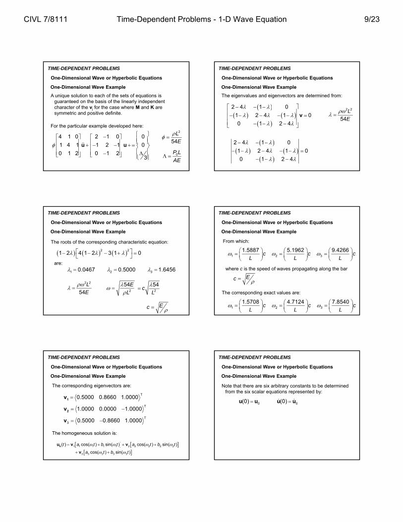
A unique solution to each of the sets of equations is guaranteed on the basis of the linearly independent character of the vj for the case where M and K are symmetric and positive definite.
For the particular example developed here:
One-Dimensional Wave Example
One-Dimensional Wave or Hyperbolic Equations
4 1 0 2 1 0 0
1 4 1 1 2 1 0
0 1 2 0 1 23
u u
2
54
L
E
0P L
AE
TIME-DEPENDENT PROBLEMS
The eigenvalues and eigenvectors are determined from:
2 4 1 0
1 2 4 1 0
0 1 2 4
v2 2
54
L
E
One-Dimensional Wave or Hyperbolic Equations
One-Dimensional Wave Example
2 4 1 0
1 2 4 1 0
0 1 2 4
TIME-DEPENDENT PROBLEMS
One-Dimensional Wave or Hyperbolic Equations
One-Dimensional Wave Example
The roots of the corresponding characteristic equation:
2 21 2 4 1 2 3 1 0
are:
1 2 30.0467 0.5000 1.6456
2 2
54
L
E
2
54E
L
2
54c
L
Ec
TIME-DEPENDENT PROBLEMS
One-Dimensional Wave or Hyperbolic Equations
One-Dimensional Wave Example
From which:
1 2 3
1.5887 5.1962 9.4266c c c
L L L
Ec
where c is the speed of waves propagating along the bar
The corresponding exact values are:
1 2 3
1.5708 4.7124 7.8540c c c
L L L
TIME-DEPENDENT PROBLEMS
One-Dimensional Wave or Hyperbolic Equations
One-Dimensional Wave Example
The corresponding eigenvectors are:
T0.5000 0.8660 1.00001v
T1.0000 0.0000 1.0000 2v
T
3 0.5000 0.8660 1.0000 v
The homogeneous solution is:
1 1 1 1 1 2 2 2 2 2
3 3 3 3 3
( ) cos( ) sin( ) cos( ) sin( )
cos( ) sin( )
t a t b t a t b t
a t b t
hu v v
v
TIME-DEPENDENT PROBLEMS
One-Dimensional Wave or Hyperbolic Equations
One-Dimensional Wave Example
Note that there are six arbitrary constants to be determined from the six scalar equations represented by:
0(0) u u 0(0) u u
CIVL 7/8111 Time-Dependent Problems - 1-D Wave Equation 9/23

TIME-DEPENDENT PROBLEMS
One-Dimensional Wave or Hyperbolic Equations
One-Dimensional Wave Example
Observe that in:T
0 0 3 p pKu Mu
a particular solution is easily obtained by taking up = d, a constant, resulting in
T
0 0 3Kd
2 1 0 0
1 2 1 0
0 1 1 3
T1 2 33
d
TIME-DEPENDENT PROBLEMS
One-Dimensional Wave or Hyperbolic Equations
One-Dimensional Wave Example
Applying the initial condition u(0) = 0 yields:
1 1 2 2 3 3(0) 0 a a a u v v v d
1
2
3
30.5000 1.0000 0.500020.8660 0.0000 0.8660 3
1.0000 1.0000 1.0000 33
a
a
a
T T
1 2 3a a a -0.8294 0.1111 0.0595 a
TIME-DEPENDENT PROBLEMS
One-Dimensional Wave or Hyperbolic Equations
One-Dimensional Wave Example
With ů(0) = ů0 = up(0) = 0, it follows that
1 1 2 2 3 3(0) 0 b b b u v v v T
1 2 3 0b b b b
The solution can then be written as:
1 1 2 20.8294 cos( ) 0.1111 cos( )t t u
v v
T
3 310.0595 cos( ) 1 2 33t v
1 1 1 1 1 2 2 2 2 2
3 3 3 3 3
( ) cos( ) sin( ) cos( ) sin( )
cos( ) sin( )
t a t b t a t b t
a t b t p
u v v
v υ
TIME-DEPENDENT PROBLEMS
One-Dimensional Wave or Hyperbolic Equations
One-Dimensional Wave Example
Recall the corresponding eigenvectors are:
T0.5000 0.8660 1.00001v
T1.0000 0.0000 1.0000 2v
T
3 0.5000 0.8660 1.0000 v
1 1 2 20.8294 cos( ) 0.1111 cos( )t t u
v v
T
3 310.0595 cos( ) 1 2 33t v
TIME-DEPENDENT PROBLEMS
One-Dimensional Wave or Hyperbolic Equations
One-Dimensional Wave Example
Substituting the eigenvectors gives:
1 2
0.5000 1.0000
0.8294 0.8660 cos( ) 0.1111 0.0000 cos( )
1.0000 1.0000
t tu
3
0.5000 110.0595 0.8660 cos( ) 23
1.0000 3
t
1 2 3
1.5887 5.1962 9.4266c c c
L L L
TIME-DEPENDENT PROBLEMS
One-Dimensional Wave or Hyperbolic Equations
One-Dimensional Wave Example
In an expanded form:
21 2 30.3333 0.4147cos( ) 0.1111cos( ) 0.0298cos( )
ut t t
31 30.6667 0.7183cos( ) 0.0516cos( )
ut t
41 2 31.0000 0.8294cos( ) 0.1111cos( ) 0.0595cos( )
ut t t
The constant term represents, in a sense, the steady-state or static solution
CIVL 7/8111 Time-Dependent Problems - 1-D Wave Equation 10/23

TIME-DEPENDENT PROBLEMS
One-Dimensional Wave or Hyperbolic Equations
One-Dimensional Wave Example
In an expanded form:
21 2 30.3333 0.4147cos( ) 0.1111cos( ) 0.0298cos( )
ut t t
31 30.6667 0.7183cos( ) 0.0516cos( )
ut t
41 2 31.0000 0.8294cos( ) 0.1111cos( ) 0.0595cos( )
ut t t
If damping were included in the physical model, the terms in the homogeneous solution corresponding to the present cosine terms would eventually damp out.
TIME-DEPENDENT PROBLEMS
One-Dimensional Wave or Hyperbolic Equations
One-Dimensional Wave Example
The corresponding exact solution can be represented in terms of the infinite series:
2
1 cos( )( , )2
n n n
n
n nL x ctu x t
L
2 1
2n
nL
( ) sin( )nn x x
TIME-DEPENDENT PROBLEMS
One-Dimensional Wave or Hyperbolic Equations
One-Dimensional Wave Example
Retaining the first three terms of the series solution at x = L/3, 2L/3, and L yields:
1 2 3
/ 3,0.3314 0.4053cos( ) 0.0901cos( ) 0.0162cos( )
u L tt t t
1 2 3
2 / 3,0.7639 0.7020cos( ) 0.0901cos( ) 0.0281cos( )
u L tt t t
1 2 3
,0.9330 0.8106cos( ) 0.0901cos( ) 0.0324cos( )
u L tt t t
where n = nc. Note the general similarity between the three-term expansion of the exact solution and the approximate solution from the three-element finite element model.
TIME-DEPENDENT PROBLEMS
One-Dimensional Wave or Hyperbolic Equations
One-Dimensional Wave Example
The approximate lowest frequency 1 is quite close to the exact lowest frequency 1, with:
The other two ratios:
1
1
1.0114
32
2 3
1.1027 1.2002
are not quite as accurate.
Recall, the general rule stating that approximately 2N unconstrained degrees of freedom are necessary in order that the first N frequencies be determined accurately. In this instance, the first frequency should be quite accurate, which is certainly the case.
TIME-DEPENDENT PROBLEMS
One-Dimensional Wave or Hyperbolic Equations
One-Dimensional Wave Example
The exact solutions u(L, t) and u4(t) are indicated for the first few oscillations below:
4u t
TIME-DEPENDENT PROBLEMS
One-Dimensional Wave or Hyperbolic Equations
One-Dimensional Wave Example
The results are for E = 3 X 10⁷ psi, = 7.5 X 10⁻⁴ Ibf-s2/in4, and L = 20 in.
4u t
CIVL 7/8111 Time-Dependent Problems - 1-D Wave Equation 11/23

TIME-DEPENDENT PROBLEMS
One-Dimensional Wave or Hyperbolic Equations
One-Dimensional Wave ExampleThe agreement is quite reasonable with the approximate
solution beginning to peak early due to the fact that all the approximate frequencies exceed the exact values.
4u t
TIME-DEPENDENT PROBLEMS
One-Dimensional Wave or Hyperbolic Equations
One-Dimensional Wave Example
A finer mesh would result in better agreement.
4u t
TIME-DEPENDENT PROBLEMS
One-Dimensional Wave or Hyperbolic Equations
One-Dimensional Wave Example
u t
TIME-DEPENDENT PROBLEMS
Time Integration Techniques – Second-Order Systems
As was the case for the systems of first-order equations, there may be situations where M and K are time-dependent or where F(t) is such that an analytical approach is not an intelligent way to proceed.
Numerical integration techniques, which are appropriate in such situations, are presented and discussed in the next sections.
One-Dimensional Wave or Hyperbolic Equations
TIME-DEPENDENT PROBLEMS
The Central Difference Method - The system of second-order linear ordinary differential equations in question is restated as:
A discretization of the time variable with tn - tn-1 = tn+1 - tn = h, the time step.
Time Integration Techniques – Second-Order Systems
One-Dimensional Wave or Hyperbolic Equations
Mu Ku F 0(0) u u 0(0) u u
1nt 1nt
u
t
nt
h h
TIME-DEPENDENT PROBLEMS
The differential equation is evaluated at t = tn to yield:
where un = u(tn) = u(nh), and Fn = F(tn) = F(nh).
Central difference representations are used for the velocity and acceleration vectors, namely,
Time Integration Techniques – Second-Order Systems
One-Dimensional Wave or Hyperbolic Equations
n n n Mu Ku F
1 1
2n n
n h
u u
u 1 12
2n n nn h
u u uu
CIVL 7/8111 Time-Dependent Problems - 1-D Wave Equation 12/23

TIME-DEPENDENT PROBLEMS
Each term is accurate to order h2. Substituting the acceleration approximation into the original equation and multiplying through by h2 and gives:
This gives a three-term recurrence relation to be used for stepping ahead in time.
A special starting procedure is necessary in that two successive u's are required in order to accomplish the solution.
Time Integration Techniques – Second-Order Systems
One-Dimensional Wave or Hyperbolic Equations
2 21 12n n n nh h Mu M K u Mu F
TIME-DEPENDENT PROBLEMS
The procedure used is as follows: the vector function u is expanded in a Taylor's series about t = 0 according to
with ü(0) computed from the differential equation evaluated at t = 0,
Time Integration Techniques – Second-Order Systems
One-Dimensional Wave or Hyperbolic Equations
2 00 0
2
hh h
uu u u
10 0 0 u M F Ku
TIME-DEPENDENT PROBLEMS
Usually M-1 is not computed; rather, the system of equations
is solved for u(0) using an LU decomposition.
The special starting value u(-h) is then given formally by
Time Integration Techniques – Second-Order Systems
One-Dimensional Wave or Hyperbolic Equations
2 1 0 0
0 02
hh h
M F Ku
u u u
0 0 0 Mu F Ku
2 10 0
1 0 0 2
hh
M F Ku
u u u
TIME-DEPENDENT PROBLEMS
The recurrence relation is then evaluated for n = 0 to yield
from which u1 is determined using u-1 and u0 from the initial conditions.
The recurrence relation is then used successively for n = 1, 2, ... until the desired time range is included.
After determining un+1, the velocity ůn and the acceleration ün at tn are computed at each time step.
Time Integration Techniques – Second-Order Systems
One-Dimensional Wave or Hyperbolic Equations
2 21 0 1 02 h h Mu M K u Mu F
TIME-DEPENDENT PROBLEMS
The entire process is summarized as:
Given: The initial conditions u(0) and ůn(0),
Time Integration Techniques – Second-Order Systems
One-Dimensional Wave or Hyperbolic Equations
10 0 0
u M F Ku
2 10 0
1 0 0 2
hh
M F Ku
u u u
Compute:
2 1 2 11 0 1 02 h h
u M K u u M F
TIME-DEPENDENT PROBLEMS
Then for n = 1, 2, …. Compute un+1 using
Time Integration Techniques – Second-Order Systems
One-Dimensional Wave or Hyperbolic Equations
2 1 2 11 12n n n nh h u M K u u M F
1 1
2n n
n h
u u
u
1 12
2n n nn h
u u uu
CIVL 7/8111 Time-Dependent Problems - 1-D Wave Equation 13/23

TIME-DEPENDENT PROBLEMS
As will be indicated later, this method is conditionally stable with the critical step size given by
Time Integration Techniques – Second-Order Systems
One-Dimensional Wave or Hyperbolic Equations
max
2crh
where (max)2 is the largest eigenvalue of the algebraic eigenvalue problem
2 0 K M x
Just as for the first-order system, values of h > hcr result in an unbounded oscillation of the numerical solution.
TIME-DEPENDENT PROBLEMS
Example: Consider the one-dimensional problem
Time Integration Techniques – Second-Order Systems
One-Dimensional Wave or Hyperbolic Equations
Define the dimensionless displacement z = kx/f0 and rewrite the differential equation as:
0mx kx f (0) 0x (0) 0x
2 2z z (0) 0z (0) 0z
where 2 = k/m.
TIME-DEPENDENT PROBLEMS
Example: It can be shown, that the recurrence relation for this one-dimensional problem is:
Time Integration Techniques – Second-Order Systems
One-Dimensional Wave or Hyperbolic Equations
2 2
1 12n n nz h z z h
with: 20z
It then follows that the starting procedure yields z-1= ½(h)2
and also that for n = 0, the recurrence relation yields z1= ½(h)2.
TIME-DEPENDENT PROBLEMS
Example: Then as outlined previously for n = 1, 2, ...,
Time Integration Techniques – Second-Order Systems
One-Dimensional Wave or Hyperbolic Equations
2 2
1 12n n nz h z z h
with:1 1
2n n
n
z zz
h
1 12
2n n nn
z z zz
h
TIME-DEPENDENT PROBLEMS
Example: For = 1, the following graph presents the results for the displacement as a function of time.
Time Integration Techniques – Second-Order Systems
One-Dimensional Wave or Hyperbolic Equations
z
TIME-DEPENDENT PROBLEMS
Example: For = 1, the following graph presents the results for the velocity as a function of time.
Time Integration Techniques – Second-Order Systems
One-Dimensional Wave or Hyperbolic Equations
z
CIVL 7/8111 Time-Dependent Problems - 1-D Wave Equation 14/23

TIME-DEPENDENT PROBLEMS
Example: For = 1, the following graph presents the results for the acceleration, as a function of time.
Time Integration Techniques – Second-Order Systems
One-Dimensional Wave or Hyperbolic Equations
z
TIME-DEPENDENT PROBLEMS
Example: The graphs present results for h = 0.1, h = 1.0, and h = 2.0.
The results for h = 0.1 are essentially the same as the exact results.
The critical step size is represented by h = 2.0 and is thus the upper limit for stability.
Values above h = 2.0 would result in unbounded oscillations.
Time Integration Techniques – Second-Order Systems
One-Dimensional Wave or Hyperbolic Equations
TIME-DEPENDENT PROBLEMS
Example: For = 1, the following graph presents the results for the displacement as a function of time (h = 2.1).
Time Integration Techniques – Second-Order Systems
One-Dimensional Wave or Hyperbolic Equations
-5.000
-4.000
-3.000
-2.000
-1.000
0.000
1.000
2.000
3.000
4.000
5.000
0 1 2 3 4 5 6 7 8 9 10
TIME-DEPENDENT PROBLEMS
Example: For = 1, the following graph presents the results for the velocity as a function of time (h = 2.1).
Time Integration Techniques – Second-Order Systems
One-Dimensional Wave or Hyperbolic Equations
-2.000
-1.500
-1.000
-0.500
0.000
0.500
1.000
1.500
2.000
0 1 2 3 4 5 6 7 8 9 10
TIME-DEPENDENT PROBLEMS
Example: For = 1, the following graph presents the results for the acceleration, as a function of time (h = 2.1).
Time Integration Techniques – Second-Order Systems
One-Dimensional Wave or Hyperbolic Equations
-5.000
-4.000
-3.000
-2.000
-1.000
0.000
1.000
2.000
3.000
4.000
5.000
0 1 2 3 4 5 6 7 8 9 10
TIME-DEPENDENT PROBLEMS
Example – Consider again the example of the one dimensional wave equation previously developed for the four-element problem:
4 1 0 2 1 0 0
1 4 1 1 2 1 0
0 1 2 0 1 2 13
v v
Time Integration Techniques – Second-Order Systems
One-Dimensional Wave or Hyperbolic Equations
m k v v F (0) 0v (0) 0v2
54
L
E
u
v
CIVL 7/8111 Time-Dependent Problems - 1-D Wave Equation 15/23
TIME-DEPENDENT PROBLEMS
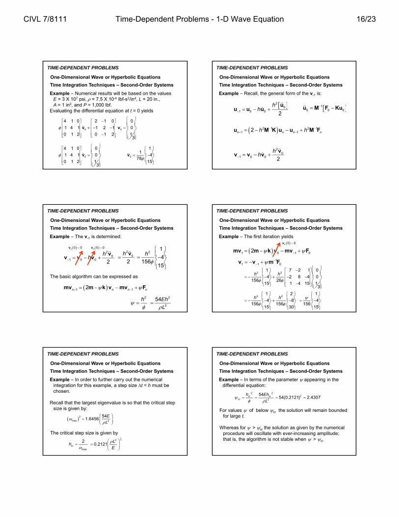
Example – Numerical results will be based on the values E = 3 X 10⁷ psi, = 7.5 X 10⁻⁴ Ibf-s2/in4, L = 20 in., A = 1 in2, and P = 1,000 lbf.
Evaluating the differential equation at t = 0 yields
0 0
4 1 0 2 1 0 0
1 4 1 1 2 1 0
0 1 2 0 1 2 13
v v
Time Integration Techniques – Second-Order Systems
One-Dimensional Wave or Hyperbolic Equations
0
4 1 0 0
1 4 1 0
0 1 2 13
v 0
11
478
15
v
TIME-DEPENDENT PROBLEMS
Example – Recall, the general form of the v-1 is:
Time Integration Techniques – Second-Order Systems
One-Dimensional Wave or Hyperbolic Equations
20
1 0 0 2
hh
uu u u
20
1 0 0 2
hh
vv v v
10 0 0
u M F Ku
2 1 2 11 12n n n nh h u M K u u M F
TIME-DEPENDENT PROBLEMS
Example – The v-1 is determined:
Time Integration Techniques – Second-Order Systems
One-Dimensional Wave or Hyperbolic Equations
20
1 0 0 2
hh
vv v v
2
0
2
h
v 21
4156
15
h
0 0 0v 0 0 0v
The basic algorithm can be expressed as
1 12n n n n mv m k v mv F
2h
2
2
54Eh
L
TIME-DEPENDENT PROBLEMS
Example – The first iteration yields
Time Integration Techniques – Second-Order Systems
One-Dimensional Wave or Hyperbolic Equations
1 0 1 02 mv m k v mv F
0 0 0v
11 1 0
v v m F
2 21 7 2 1 0
4 2 8 4 0156 26
15 1 4 15 13
h h
2 21 2
4 8156 156
15 30
h h
1
4156
15
TIME-DEPENDENT PROBLEMS
Example – In order to further carry out the numerical integration for this example, a step size t = h must be chosen.
Recall that the largest eigenvalue is so that the critical step size is given by:
Time Integration Techniques – Second-Order Systems
One-Dimensional Wave or Hyperbolic Equations
2
max 2
541.6456
E
L
The critical step size is given by
max
2crh
122
0.2121L
E
TIME-DEPENDENT PROBLEMS
Example – In terms of the parameter appearing in the differential equation:
Time Integration Techniques – Second-Order Systems
One-Dimensional Wave or Hyperbolic Equations
For values of below cr the solution will remain bounded for large t.
Whereas for > cr the solution as given by the numerical procedure will oscillate with ever-increasing amplitude; that is, the algorithm is not stable when > cr
2cr
cr
h
2
2
54 crEh
L 254(0.2121) 2.4307
CIVL 7/8111 Time-Dependent Problems - 1-D Wave Equation 16/23

TIME-DEPENDENT PROBLEMS
Example – As was seen from the analytical solution presented previously, all of the frequencies determined from K - 2M = 0 are contained in the solution.
In order to obtain numerical results that accurately contain the effects of all the frequency components, it is necessary to choose a step size that is relatively small compared with the period of the largest frequency.
A rule of thumb is to break half the period of the largest frequency into 10 equal intervals; that is, take:
Time Integration Techniques – Second-Order Systems
One-Dimensional Wave or Hyperbolic Equations
*
max10h
TIME-DEPENDENT PROBLEMS
Example – For the present example
Time Integration Techniques – Second-Order Systems
One-Dimensional Wave or Hyperbolic Equations
*
max10h
94.267
L
c
with the parameter given by
2* h
2
94.267L
c
2
2
54
94.267
L E
c L
0.05998
TIME-DEPENDENT PROBLEMS
Example – Results for this example for h1 = 4.2433(10-6) sec and h2 = 2.1216(10-5) sec.
The critical step size is h2 and h1 = h2 /5 is a value somewhat larger than the one corresponding to dividing the half period of the maximum frequency into 10 equal segments.
Time Integration Techniques – Second-Order Systems
One-Dimensional Wave or Hyperbolic Equations
TIME-DEPENDENT PROBLEMS
The displacement at x = L, that is, u4(t) is shown below
Time Integration Techniques – Second-Order Systems
One-Dimensional Wave or Hyperbolic Equations
TIME-DEPENDENT PROBLEMS
The analytical solution and the central difference numerical solution for t = h = 4.2433(10-6) sec. agree well.
Time Integration Techniques – Second-Order Systems
One-Dimensional Wave or Hyperbolic Equations
TIME-DEPENDENT PROBLEMS
Example – The velocity at x = L is:
Time Integration Techniques – Second-Order Systems
One-Dimensional Wave or Hyperbolic Equations
CIVL 7/8111 Time-Dependent Problems - 1-D Wave Equation 17/23

TIME-DEPENDENT PROBLEMS
Example – The acceleration at x = L is:
Time Integration Techniques – Second-Order Systems
One-Dimensional Wave or Hyperbolic Equations
TIME-DEPENDENT PROBLEMS
Generally, the accuracy of the results improves with an increase in the number of elements used.
This can be traced to the fact that more of the approximate eigenvalues corresponding to the exact solution are more accurately determined using more elements.
The use of higher-order interpolations may also result in some improvement in accuracy, although not to the same extent as increasing the number of linearly interpolated elements.
Time Integration Techniques – Second-Order Systems
One-Dimensional Wave or Hyperbolic Equations
TIME-DEPENDENT PROBLEMS
As is apparent from the results of the example, that all three of the frequencies contribute to the solution.
This means that the combined requirements of not exceeding the critical time step and integrating the effects of the higher modes accurately can lead to a very small h, and hence an expensive algorithm.
Fortunately for large systems the higher modes do not contribute significantly to the solution so that an unconditionally stable algorithm with a larger time step can be used satisfactorily.
Time Integration Techniques – Second-Order Systems
One-Dimensional Wave or Hyperbolic Equations
TIME-DEPENDENT PROBLEMS
Finally, it is easily seen that if lumped mass matrices are used, M is a diagonal matrix and the computations involved in the central difference algorithm reduce at each step to a matrix multiplication and vector additions, that is, no solution of a set of algebraic equations is required at each step.
Time Integration Techniques – Second-Order Systems
One-Dimensional Wave or Hyperbolic Equations
TIME-DEPENDENT PROBLEMS
NEWMARK'S METHOD - Newmark's method is based on an extension of the average acceleration method, which is conditionally stable.
Newmark was able to generalize the algorithm so as to retain its simple form, yet produce an unconditionally stable algorithm.
Time Integration Techniques – Second-Order Systems
One-Dimensional Wave or Hyperbolic Equations
TIME-DEPENDENT PROBLEMS
NEWMARK'S METHOD - The average acceleration method is based on the assumption that over a small time increment any nodal acceleration can be considered to be a linear function of time.
Time Integration Techniques – Second-Order Systems
One-Dimensional Wave or Hyperbolic Equations
t
u t
t
t h
hu
u
CIVL 7/8111 Time-Dependent Problems - 1-D Wave Equation 18/23

TIME-DEPENDENT PROBLEMS
NEWMARK'S METHOD - For the interval 0 < < h, the interval corresponding to the time step, the acceleration is expressed as
Time Integration Techniques – Second-Order Systems
One-Dimensional Wave or Hyperbolic Equations
1t t t hh h
u u u
2 2
2 2t t t t hh h
u u u u
Integrating yields
TIME-DEPENDENT PROBLEMS
NEWMARK'S METHOD – If = h, then
Time Integration Techniques – Second-Order Systems
One-Dimensional Wave or Hyperbolic Equations
2
t t ht t
h
u uu u
That is, the increment in the velocity is based on the approximate average acceleration on the interval (0, h).
Integrating yields
t averageh u u
2 3 3
2 6 6t t t t t hh h
u u u u u
TIME-DEPENDENT PROBLEMS
NEWMARK'S METHOD – These expressions are employed with the differential equations
Time Integration Techniques – Second-Order Systems
One-Dimensional Wave or Hyperbolic Equations
to yield the conditionally stable average acceleration algorithm. Newmark generalized Equations
Mu Ku F
1t h t t t h h u u u u
21
2t h t t t t hh h
u u u u u
TIME-DEPENDENT PROBLEMS
NEWMARK'S METHOD – Newmark generalized equations
Time Integration Techniques – Second-Order Systems
One-Dimensional Wave or Hyperbolic Equations
The method is unconditionally stable as long as the parameters and are chosen to satisfy 0.5 and 0.25( + 0.5)2.
Note that = ½ and =¼ corresponds to the average acceleration method.
1t h t t t h h u u u u
21
2t h t t t t hh h
u u u u u
TIME-DEPENDENT PROBLEMS
NEWMARK'S METHOD – The equation for ut+h is solved for üt+h and substituted into the equation for ůt+h to yield
Time Integration Techniques – Second-Order Systems
One-Dimensional Wave or Hyperbolic Equations
where c2 = 1 - /2 and then into the differential equation evaluated at t + h to yield
2
t h t tt h t t
hc h
h
u u uu u u
21t h t t t t hh h c h h M K u M u u u F
where c1 = 1/2 -
TIME-DEPENDENT PROBLEMS
NEWMARK'S METHOD – This equation, together with the two equations for the velocity and acceleration at t + h, can be used to step ahead in time to determine the solution
Time Integration Techniques – Second-Order Systems
One-Dimensional Wave or Hyperbolic Equations
2
t h t tt h t t
hc h
h
u u uu u u
21t h t t t t hh h c h h M K u M u u u F
12
t h t t tt h
h c
h
u u u uu
CIVL 7/8111 Time-Dependent Problems - 1-D Wave Equation 19/23

TIME-DEPENDENT PROBLEMS
NEWMARK'S METHOD – In order to start the process, the acceleration at t = 0 is needed and is determined by solving the governing equations evaluated at t = 0,
Time Integration Techniques – Second-Order Systems
One-Dimensional Wave or Hyperbolic Equations
0 0 0 Mu F Ku
for acceleration ü(0), the previous equations are then used to step ahead using the unconditionally stable Newmark algorithm.
TIME-DEPENDENT PROBLEMS
Time Integration Techniques – Second-Order Systems
One-Dimensional Wave or Hyperbolic Equations
Given: The initial conditions u(0) and ůn(0),
Compute: ü(0), then un,ůn, and ün, for n = 1, 2, …..
NEWMARK'S METHOD – The algorithm consists of:
21 1 1n n n n nh h c h h M K u M u u u F
11 2
n n nn n n
hc h
h
u u uu u u
1 11 2
n n n nn
h c
h
u u u uu
TIME-DEPENDENT PROBLEMS
Time Integration Techniques – Second-Order Systems
One-Dimensional Wave or Hyperbolic Equations
Specifically, with u0, ů0, and ü0 known
NEWMARK'S METHOD – The algorithm consists of:
21 0 0 1 0 1h h c h h M K u M u u u F
1 0 01 0 2 0
hc h
h
u u uu u u
1 0 0 1 01 2
h c
h
u u u u
u
TIME-DEPENDENT PROBLEMS
Time Integration Techniques – Second-Order Systems
One-Dimensional Wave or Hyperbolic Equations
Then with u1,ů1, and ü1 known
NEWMARK'S METHOD – The algorithm consists of:
22 1 1 1 1 2h h c h h M K u M u u u F
2 1 12 1 2 1
hc h
h
u u u
u u u
2 1 1 1 12 2
h c
h
u u u u
u
TIME-DEPENDENT PROBLEMS
Time Integration Techniques – Second-Order Systems
One-Dimensional Wave or Hyperbolic Equations
NEWMARK'S METHOD – The algorithm is continued until the time range of interest is covered.
Note that for the Newmark algorithm, lumping of the mass matrix results in no computational advantage.
TIME-DEPENDENT PROBLEMS
Example – Consider again the example of the one dimensional wave equation previously developed for the four-element problem:
4 1 0 2 1 0 0
1 4 1 1 2 1 06
0 1 2 0 1 2 13
v v
Time Integration Techniques – Second-Order Systems
One-Dimensional Wave or Hyperbolic Equations
mv kv F (0) 0v (0) 0v2
9
L
E
u
v
CIVL 7/8111 Time-Dependent Problems - 1-D Wave Equation 20/23

TIME-DEPENDENT PROBLEMS
Time Integration Techniques – Second-Order Systems
One-Dimensional Wave or Hyperbolic Equations
NEWMARK'S METHOD – The equations to be solved at the first step can be written as
21 0 0 1 0 1h c h m k v m v v v f
1 0 01 0 2 0
hc h
h
v v vv v v
1 0 0 1 01 2
h c
h
v v v v
v
2h
TIME-DEPENDENT PROBLEMS
Time Integration Techniques – Second-Order Systems
One-Dimensional Wave or Hyperbolic Equations
NEWMARK'S METHOD – Evaluating the differential equation at t = 0 yields
0 0 mv f kv 1
0 0
m
v f kv
0
7 2 1 01
2 8 4 026
1 4 15 13
v1
14
7815
8
0.6923
10 2.7692
10.3846
Numerical results will be based on the values: E = 3 X 10⁷ psi, = 7.5 X 10⁻⁴ Ibf-s2/in4, and L = 20 in.
TIME-DEPENDENT PROBLEMS
Time Integration Techniques – Second-Order Systems
One-Dimensional Wave or Hyperbolic Equations
NEWMARK'S METHOD – Taking = 0.25, = 0.5, and h = 4.2422 x 10⁻⁶ seconds yield
1
0.6748 0.1626 0.0000
0.1626 0.6748 0.1626
0.0000 0.1626 0.3374
m k v
0.0000
0.0000
0.0081
f
At step 1:
21 0
0.6748 0.1626 0.0000 0.0000
0.1626 0.6748 0.1626 0.25 0.0000
0.0000 0.1626 0.3374 0.0081
h
v m v
21 0 0 1 0 1h c h m k v m v v v f
TIME-DEPENDENT PROBLEMS
Time Integration Techniques – Second-Order Systems
One-Dimensional Wave or Hyperbolic Equations
NEWMARK'S METHOD – The solution for v1 is
1 0 01 0 2 0
hc h
h
v v vv v v
0 0 0v
0 0 0v
Now solve for the velocity at t = 0
11 h
v
v
1 0.0006 0.0023 0.0091T
v
410 0.0265 0.1101 0.4304T
1 0 0 1 01 2
h c
h
v v v v
v
TIME-DEPENDENT PROBLEMS
Time Integration Techniques – Second-Order Systems
One-Dimensional Wave or Hyperbolic Equations
NEWMARK'S METHOD – The equation for acceleration at t = 0 is
0 0 0v
0 0 0v
Now solve for the acceleration at t = h
12h
v
81 10 0.5585 2.4209 9.9008
T v
TIME-DEPENDENT PROBLEMS
Time Integration Techniques – Second-Order Systems
One-Dimensional Wave or Hyperbolic Equations
NEWMARK'S METHOD – After step 2:
2 0.0020 0.0087 0.0357T
v
42 10 0.0423 0.1918 0.8211
T v
82 10 0.1848 1.4300 8.5155
T v
CIVL 7/8111 Time-Dependent Problems - 1-D Wave Equation 21/23

TIME-DEPENDENT PROBLEMS
Time Integration Techniques – Second-Order Systems
One-Dimensional Wave or Hyperbolic Equations
NEWMARK'S METHOD – The results for further integration are presented in following figures. The step size h1 = 4.2433 x 10⁻⁶ sec indicated above is the same as the smaller of the two values used for the central difference algorithm in the previous section.
Integrations are also carried out for h2 = 4.2433 x 10⁻⁵ sec = 10h1, a value twice that of the critical value for the central difference algorithm of the previous section. In all the figures, the abscissa n represents the number of time steps of length h1.
TIME-DEPENDENT PROBLEMS
Time Integration Techniques – Second-Order Systems
One-Dimensional Wave or Hyperbolic Equations
NEWMARK'S METHOD – Displacement at x = L
TIME-DEPENDENT PROBLEMS
Time Integration Techniques – Second-Order Systems
One-Dimensional Wave or Hyperbolic Equations
NEWMARK'S METHOD – Velocity at x = L
TIME-DEPENDENT PROBLEMS
Time Integration Techniques – Second-Order Systems
One-Dimensional Wave or Hyperbolic Equations
NEWMARK'S METHOD – Acceleration at x = L
TIME-DEPENDENT PROBLEMS
Time Integration Techniques – Second-Order Systems
One-Dimensional Wave or Hyperbolic Equations
NEWMARK'S METHOD – The results for displacement indicate that for h = h1, there is very good agreement between the numerical solution and the corresponding analytical solution, both comparing favorably with the exact solution.
For h = h2, the unconditionally stable Newmark algorithm is unable to predict the part of the response arising from the higher frequencies, but is able to predict the essential character of the displacement at the end x = L.
TIME-DEPENDENT PROBLEMS
Time Integration Techniques – Second-Order Systems
One-Dimensional Wave or Hyperbolic Equations
NEWMARK'S METHOD – The results velocity at x = Lindicate a rough similarity between the analytical solution and the Newmark solution for h = h1.
Similarly, the numerical results for h = h2 bear some resemblance to the analytical and exact solutions, but are neither qualitatively nor quantitatively satisfactory.
The results for the accelerations, as was the case for the central difference algorithm, completely unsatisfactory.
CIVL 7/8111 Time-Dependent Problems - 1-D Wave Equation 22/23

End of
1-D Time Dependent
Problems – Part b
CIVL 7/8111 Time-Dependent Problems - 1-D Wave Equation 23/23
Related Documents