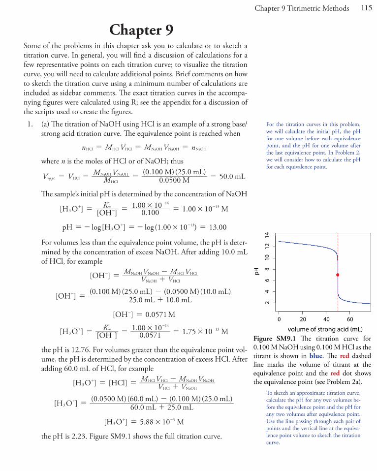
115 Chapter 9 Titrimetric Methods Chapter 9 Some of the problems in this chapter ask you to calculate or to sketch a titration curve. In general, you will find a discussion of calculations for a few representative points on each titration curve; to visualize the titration curve, you will need to calculate additional points. Brief comments on how to sketch the titration curve using a minimum number of calculations are included as sidebar comments. e exact titration curves in the accompa- nying figures were calculated using R; see the appendix for a discussion of the scripts used to create the figures. 1. (a) e titration of NaOH using HCl is an example of a strong base/ strong acid titration curve. e equivalence point is reached when n M V M V n HCl HCl HCl NaOH NaOH NaOH = = = where n is the moles of HCl or of NaOH; thus V V M M V 0.0500 M (0.100 M) (25.0 mL) 50.0 mL . . eq pt HCl HCl NaOH NaOH = = = = e sample’s initial pH is determined by the concentration of NaOH [ ] [ ] . . . K 0 100 1 00 10 1 00 10 HO OH M 14 13 3 w # # = = = + - - - pH log[H O ] log (1.00 10 ) 13.00 3 13 # =- =- = + - For volumes less than the equivalence point volume, the pH is deter- mined by the concentration of excess NaOH. After adding 10.0 mL of HCl, for example [ ] V V M V M V OH NaOH HCl NaOH NaOH HCl HCl = + - - [OH] 25.0 mL 10.0 mL (0.100 M) (25.0 mL) (0.0500 M) (10.0 mL) = + - - [ ] . 0 0571 OH M = - [ ] [ ] . . . K 0 1 00 10 1 10 0571 75 HO OH M 14 13 3 w # # = = = + - - - the pH is 12.76. For volumes greater than the equivalence point vol- ume, the pH is determined by the concentration of excess HCl. After adding 60.0 mL of HCl, for example [ V V M V M V HO] [HCl] 3 HCl NaOH HCl HCl NaOH NaOH = = + - + 60 25 05 0 60 1 25 [H O ] .0 mL .0 mL (0. 0 M)( .0 mL) (0. 00 M) ( .0 mL) 3 = + - + [ ] . 5 88 10 HO M 3 3 # = + - the pH is 2.23. Figure SM9.1 shows the full titration curve. To sketch an approximate titration curve, calculate the pH for any two volumes be- fore the equivalence point and the pH for any two volumes after equivalence point. Use the line passing through each pair of points and the vertical line at the equiva- lence point volume to sketch the titration curve. 0 20 40 60 2 4 6 8 10 12 14 volume of strong acid (mL) pH Figure SM9.1 e titration curve for 0.100 M NaOH using 0.100 M HCl as the titrant is shown in blue. e red dashed line marks the volume of titrant at the equivalence point and the red dot shows the equivalence point (see Problem 2a). For the titration curves in this problem, we will calculate the initial pH, the pH for one volume before each equivalence point, and the pH for one volume after the last equivalence point. In Problem 2, we will consider how to calculate the pH for each equivalence point.

Welcome message from author
This document is posted to help you gain knowledge. Please leave a comment to let me know what you think about it! Share it to your friends and learn new things together.
Transcript
115Chapter 9 Titrimetric Methods
Chapter 9Some of the problems in this chapter ask you to calculate or to sketch a titration curve. In general, you will find a discussion of calculations for a few representative points on each titration curve; to visualize the titration curve, you will need to calculate additional points. Brief comments on how to sketch the titration curve using a minimum number of calculations are included as sidebar comments. The exact titration curves in the accompa-nying figures were calculated using R; see the appendix for a discussion of the scripts used to create the figures.1. (a) The titration of NaOH using HCl is an example of a strong base/
strong acid titration curve. The equivalence point is reached when
n M V M V nHCl HCl HCl NaOH NaOH NaOH= = =
where n is the moles of HCl or of NaOH; thus
V V MM V
0.0500 M(0.100 M)(25.0 mL) 50.0 mL. .eq pt HCl
HCl
NaOH NaOH= = = =
The sample’s initial pH is determined by the concentration of NaOH
[ ] [ ] .. .K
0 1001 00 10 1 00 10H O OH M
1413
3w # #= = =+-
--
pH log[H O ] log(1.00 10 ) 13.00313#=- =- =+ -
For volumes less than the equivalence point volume, the pH is deter-mined by the concentration of excess NaOH. After adding 10.0 mL of HCl, for example
[ ] V VM V M VOH
NaOH HCl
NaOH NaOH HCl HCl= +--
[OH ] 25.0 mL 10.0 mL(0.100 M)(25.0 mL) (0.0500 M)(10.0 mL)
= +--
[ ] .0 0571OH M=-
[ ] [ ] .. .K0
1 00 10 1 100571 75H O OH M14
133
w # #= = =+-
--
the pH is 12.76. For volumes greater than the equivalence point vol-ume, the pH is determined by the concentration of excess HCl. After adding 60.0 mL of HCl, for example
[ V VM V M VH O ] [HCl]3
HCl NaOH
HCl HCl NaOH NaOH= = +-+
60 2505 0 60 1 25[H O ] .0 mL .0 mL
(0. 0 M)( .0 mL) (0. 00 M)( .0 mL)3 =
+-+
[ ] .5 88 10H O M33 #=+ -
the pH is 2.23. Figure SM9.1 shows the full titration curve.
To sketch an approximate titration curve, calculate the pH for any two volumes be-fore the equivalence point and the pH for any two volumes after equivalence point. Use the line passing through each pair of points and the vertical line at the equiva-lence point volume to sketch the titration curve.
0 20 40 60
24
68
1012
14
volume of strong acid (mL)
pH
Figure SM9.1 The titration curve for 0.100 M NaOH using 0.100 M HCl as the titrant is shown in blue. The red dashed line marks the volume of titrant at the equivalence point and the red dot shows the equivalence point (see Problem 2a).
For the titration curves in this problem, we will calculate the initial pH, the pH for one volume before each equivalence point, and the pH for one volume after the last equivalence point. In Problem 2, we will consider how to calculate the pH for each equivalence point.
116 Solutions Manual for Analytical Chemistry 2.1
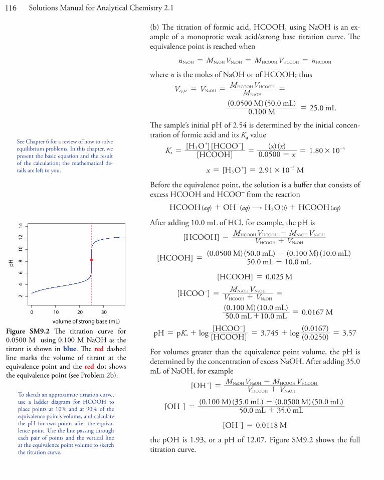
(b) The titration of formic acid, HCOOH, using NaOH is an ex-ample of a monoprotic weak acid/strong base titration curve. The equivalence point is reached when
n M V M V nNaOH NaOH NaOH HCOOH HCOOH HCOOH= = =
where n is the moles of NaOH or of HCOOH; thus
.
V V MM V
105 50 250 00 M
(0. 00 M)( .0 mL) .0 mL
. .eq pt NaOHNaOH
HCOOH HCOOH= = =
=
The sample’s initial pH of 2.54 is determined by the initial concen-tration of formic acid and its Ka value
.( ) ( ) .K xx x
0 0500 1 80 10[HCOOH][H O ][HCOO ] 4
a3 #= = - =
+ --
[ ] .x 2 91 10H O M33 #= =+ -
Before the equivalence point, the solution is a buffer that consists of excess HCOOH and HCOO– from the reaction
( ) ( ) ( ) ( )aq aq l aqHCOOH OH H O HCOOH2$+ +-
After adding 10.0 mL of HCl, for example, the pH is
V VM V M V[HCOOH]
HCOOH NaOH
HCOOH HCOOH NaOH NaOH= +-
[HCOOH] 50.0 mL 10.0 mL(0.0500 M)(50.0 mL) (0.100 M)(10.0 mL)
= +-
[HCOOH] 0.025 M=
]
.
V VM V
0 0167
[HCOO
50.0 mL 10.0 mL(0.100 M)(10.0 mL) M
HCOOH NaOH
NaOH NaOH= + =
+ =
-
. ( . )( . ) .log logK 3 745 0 02500 0167 3 57pH p [HCOOH]
[HCOO ]a= + = + =
-
For volumes greater than the equivalence point volume, the pH is determined by the concentration of excess NaOH. After adding 35.0 mL of NaOH, for example
[ V VM V M VOH ]
HCOOH NaOH
NaOH HCOOHNaOH HCOOH= +--
50 3510 35 05 50[OH ] .0 mL .0 mL
(0. 0 M)( .0 mL) (0. 00 M)( .0 mL)= +
--
[ ] .0 0118OH M=-
the pOH is 1.93, or a pH of 12.07. Figure SM9.2 shows the full titration curve.
See Chapter 6 for a review of how to solve equilibrium problems. In this chapter, we present the basic equation and the result of the calculation; the mathematical de-tails are left to you.
0 10 20 30
24
68
1012
14
volume of strong base (mL)
pH
Figure SM9.2 The titration curve for 0.0500 M using 0.100 M NaOH as the titrant is shown in blue. The red dashed line marks the volume of titrant at the equivalence point and the red dot shows the equivalence point (see Problem 2b).
To sketch an approximate titration curve, use a ladder diagram for HCOOH to place points at 10% and at 90% of the equivalence point’s volume, and calculate the pH for two points after the equiva-lence point. Use the line passing through each pair of points and the vertical line at the equivalence point volume to sketch the titration curve.
117Chapter 9 Titrimetric Methods
(c) The titration of ammonia, NH3, using HCl is an example of a monoprotic weak base/strong acid titration curve. The equivalence point is reached when
n M V M V nHCl HCl HCl NH NHNH 3 33= = =
where n is the moles of HCl or of NH3; thus
.
V V MM V
11 50 500 00 M
(0. 00 M)( .0 mL) .0 mL
. .eq pt HClHCl
NH NH33= = =
=
The sample’s initial pOH of 2.88, or a pH of 11.12, is determined by the initial concentration of ammonia and its Kb value
.( ) ( ) .K xx x
0 100 1 75 10[NH ][OH ][NH ] 5
b3
4 #= = - =- +
-
[ ] .x 101 31OH M3#= =- -
Before the equivalence point, the solution is a buffer that consists of excess NH3 and NH4
+ from the reaction
( ) ( ) ( ) ( )aq aq l aqH O H ONH NH3 43 2$+ ++ +
After adding 20.0 mL of HCl, for example, the pH is
V VM V M V[ ]NH3
NH HCl
NH HClNH HCl
3
33= +-
21 2[ ] 50.0 mL 0.0 mL
(0. 00 M)(50.0 mL) (0.100 M)( 0.0 mL)NH3 = +-
.0 0429[ ] MNH3 =
]
.
V VM V
22 0 0286
[NH
50.0 mL 0.0 mL(0.100 M)( 0.0 mL) M
4HCl
HCl HCl
NH3
= + =
+ =
+
( . )( . ). .log logK 0 02860 04299 244 9 42pH p [ ]
[ ]NHNH
a4
3= + = + =+
For volumes greater than the equivalence point volume, the pH is determined by the amount of excess HCl. After adding 60.0 mL of HCl, for example
[ V VM V M VH O ]3
NH HCl
HCl NHHCl NH
3
33= +-+
50 6010 60 1 50[H O ] .0 mL .0 mL
(0. 0 M)( .0 mL) (0. 00 M)( .0 mL)3 =
+-+
[ ] .0 00909H O M3 =+
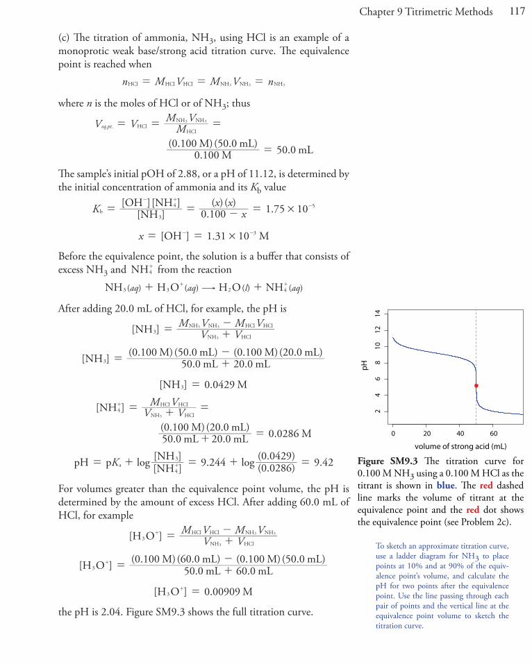
the pH is 2.04. Figure SM9.3 shows the full titration curve.
Figure SM9.3 The titration curve for 0.100 M NH3 using a 0.100 M HCl as the titrant is shown in blue. The red dashed line marks the volume of titrant at the equivalence point and the red dot shows the equivalence point (see Problem 2c).
To sketch an approximate titration curve, use a ladder diagram for NH3 to place points at 10% and at 90% of the equiv-alence point’s volume, and calculate the pH for two points after the equivalence point. Use the line passing through each pair of points and the vertical line at the equivalence point volume to sketch the titration curve.
0 20 40 60
24
68
1012
14
volume of strong acid (mL)
pH
118 Solutions Manual for Analytical Chemistry 2.1
(d) The titration of ethylenediamine, which we abbreviate here as en, using HCl is an example of a diprotic weak base/strong acid titration curve. Because en is diprotic, the titration curve has two equivalence points; the first equivalence point is reached when
n M V M V nHCl HCl HCl en enen= = =
where n is the moles of HCl or of en; thus
.
V V MM V
105 0 50 250 00 M
(0. 0 M)( .0 mL) .0 mL
1eq.pt. HClHCl
en en= = =
=
The second equivalence point is reached after adding an additional 25.0 mL of HCl, for a total volume of 50.0 mL.
The sample’s initial pOH of 2.69, or a pH of 11.31, is determined by the initial concentration of en and its Kb1 value
.( ) ( ) .K xx x
0 0500 8 47 10[en][OH ][Hen ]
15
b #= = - =- +
-
[ ] .x 102 06OH M3#= =- -
Before the first equivalence point the pH is fixed by an Hen+/en buffer; for example, after adding 10.0 mL of HCl, the pH is
V VM V M V[en]
en HCl
en en HCl HCl= +-
105 0 1[en] 50.0 mL 0.0 mL
(0. 0 M)(50.0 mL) (0.100 M)( 0.0 mL)= +
-
.0 0250[ ] Men =
]
.
V VM V
0 011 167
[Hen
50.0 mL 0.0 mL(0.100 M)( 0.0 mL) M
HCl
HCl HCl
en= + =
+ =
+
. ( . )( . ) .log logK 9 928 0 01670 0250 10 10pH p [Hen ]
[en]2a= + = + =+
Between the two equivalence points, the pH is fixed by a buffer of H2en2+ and en; for example, after adding 35.0 mL of HCl the pH is
( )V V
M V M V V[Hen ]en HCl
en en HCl HCl eq.pt.1= +
- -+
.35
05 0 35 25 0[Hen ] 50.0 mL .0 mL(0. 0 M)(50.0 mL) (0.100 M)( .0 mL)
= +- -+
.0 0176[ ] MHen =+
] ( )V V
M V V[H en22
en HCl
HCl HCl eq.pt.1= +
-+
Be sure to use pKa2 in the Hender-son-Hasselbach equation, not pKa1, as the latter describes the acid-base equilibrium between H2en2+ and Hen+.
119Chapter 9 Titrimetric Methods
] . )35
35 025[H en 50.0 mL .0 mL(0.100 M)( .0 mL
22 = +
-+
] .0 0118[H en M22 =+
( . )( . ). .log logK 0 01180 06 848 176 7 02pH p [H en ]
[Hen ]1
22a= + = + =+
+
For volumes greater than the second equivalence point volume, the pH is determined by the concentration of excess HCl. After adding 60.0 mL of HCl, for example
[ ( )V V
M V VH O ]3en HCl
HCl HCl eq.pt2= +
-+
50 6010 60 50[H O ] .0 mL .0 mL
(0. 0 M)( .0 .0 mL)3 =
+-+
[ ] .0 00909H O M3 =+
the pH is 2.04. Figure SM9.4 shows the full titration curve. (e) The titration of citric acid, which we abbreviate here as H3A, using
NaOH is an example of a triprotic weak acid/strong base titration curve. Because H3A is triprotic, the titration curve has three equiva-lence points; the first equivalence point is reached when
n M V M V nNaOH NaOH NaOH H A H A H A3 3 2= = =
where n is the moles of HCl or of H3A; thus
. .
V V MM M
1204 0 50 16 70 0 M
(0. 0 M)( .0 mL) mL
eq.pt.1 NaOHNaOH
H A H A3 3= = =
=
The second equivalence point occurs after adding an additional 16.7 mL of HCl, for a total volume of 33.33 mL, and the third equivalence point after adding an additional 16.7 mL of HCl, for a total volume of 50.0 mL.
The sample’s initial pH of 2.29 is determined by the initial concen-tration of citric acid and its Ka1 value
.( ) ( ) .K xx x
0 0 00 104 7 45[ ][H O ][ ]
H AH A
14
a3
3
2 #= =-
=+ -
-
[ ] .x 105 10H O M33 #= =+ -
Adding NaOH creates, in succession, an H3A/H2A– buffer, an H2A–/HA2– buffer, and an HA2–/A3– buffer. We can calculate the pH in these buffer regions using the same approach outlined in the pre-vious three problems; however, because citric acid’s pKa values are sufficiently similar in value (see Figure SM9.5) we must be careful to avoid pHs where two buffer regions overlap. After adding 5.00 mL of NaOH, for example, the pH is
0 20 40 60
24
68
1012
14
volume of strong acid (mL)
pH
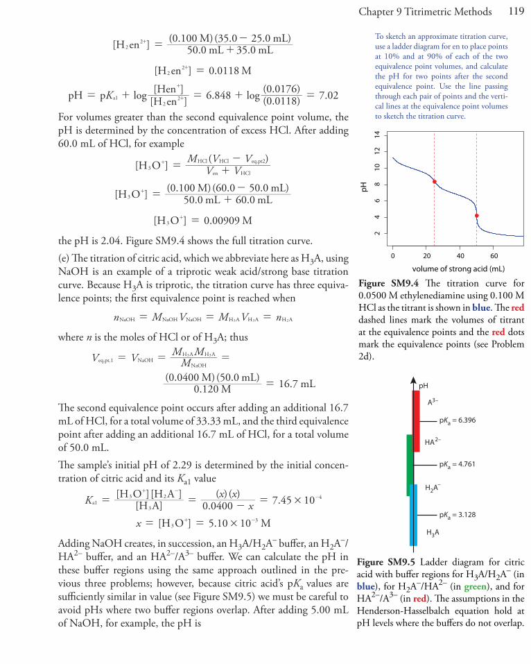
Figure SM9.4 The titration curve for 0.0500 M ethylenediamine using 0.100 M HCl as the titrant is shown in blue. The red dashed lines mark the volumes of titrant at the equivalence points and the red dots mark the equivalence points (see Problem 2d).
To sketch an approximate titration curve, use a ladder diagram for en to place points at 10% and at 90% of each of the two equivalence point volumes, and calculate the pH for two points after the second equivalence point. Use the line passing through each pair of points and the verti-cal lines at the equivalence point volumes to sketch the titration curve.
H3A
pKa = 3.128
pKa = 4.761
pKa = 6.396
H2A–
HA2–
A3–
pH
Figure SM9.5 Ladder diagram for citric acid with buffer regions for H3A/H2A– (in blue), for H2A–/HA2– (in green), and for HA2–/A3– (in red). The assumptions in the Henderson-Hasselbalch equation hold at pH levels where the buffers do not overlap.
120 Solutions Manual for Analytical Chemistry 2.1
V VM V M V[H A]3
H A NaOH
H A NaOH NaOHH A
3
33= +-
2[H A] 50.0 mL 5.00 mL(0.0400 M)(50.0 mL) (0.1 0 M)(5.00 mL)
3 = +-
[ ] 0.0255 MH A3 =
]
.
V VM V
5 02 5 0 0 0109
[H A
50.0 mL . 0 mL(0.1 0 M)( . 0 mL) M
2H A NaOH
NaOH NaOH
3
= + =
+ =
-
. ( . )( . ) .log logK 3 128 0 02550 0109 2 76pH p [H A]
[H A ]1a
3
2= + = + =-
After adding 30.00 mL of NaOH the pH is(
V VM V M V V[H A ] )
2H A NaOH
H A H A NaOH NaOH eq.pt.1
3
3 3= +
- --
.3
30 16 70
2[H A ] 50.0 mL .0 mL(0.0400 M)(50.0 mL) (0.1 0 M)( .0 mL)
2 = +- --
.5 05 10[H A ] M23#=- -
] ( )V V
M V V[HA2
H A NaOH
NaOH NaOH eq.pt.1
3
= +--
.16 7[HA ] 50.0 mL 30.0 mL(0.120 M)(30.0 mL)2 = +
--
200[HA ] 0.0 M2 =-
. ( . )( . ) .log logK 4 761 0 00500 0200 5 365pH p [H A ]
[HA ]2
2
2
a= + = + =-
-
and after adding 45.0 mL of NaOH the pH is( )
V VM V M V V[HA ]2
H A NaOH
H A H A NaOH NaOH eq.pt.2
3
3 3= +
- --
.452 4 33 3[HA ] 50.0 mL .0 mL
(0.0400 M)(50.0 mL) (0.1 0 M)( 5.0 mL)2 =+
- --
0627[HA ] 0.0 M2 =-
] ( )V V
M V V[A3
H A NaOH
NaOH NaOH eq.pt.2
3
= +--
.45
45 33 3[A ] 50.0 mL .0 mL(0.120 M)( .0 mL)3 =
+--
148[A ] 0.0 M3 =-
. ( . )( . ) .log logK 6 396 0 006270 0148 6 77pH p [HA ]
[A ]3 2
3
a= + = + =-
-
121Chapter 9 Titrimetric Methods
For volumes greater than the third equivalence point volume, the pH is determined by the concentration of excess NaOH. After adding 60.0 mL of NaOH, for example
[ ( )V V
M V VOH ]H A NaOH
NaOH NaOH eq.pt.3
3
= +--
50 6012 60 50[OH ] .0 mL .0 mL
(0. 0 M)( .0 .0 mL)=
+--
[ ] .0 0109OH M=-
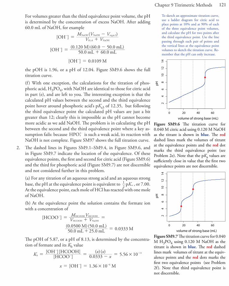
the pOH is 1.96, or a pH of 12.04. Figure SM9.6 shows the full titration curve.
(f ) With one exception, the calculations for the titration of phos-phoric acid, H3PO4, with NaOH are identical to those for citric acid in part (e), and are left to you. The interesting exception is that the calculated pH values between the second and the third equivalence point hover around phosphoric acid’s pKa3 of 12.35, but following the third equivalence point the calculated pH values are just a bit greater than 12; clearly this is impossible as the pH cannot become more acidic as we add NaOH. The problem is in calculating the pH between the second and the third equivalence point where a key as-sumption fails: because HPO4
2- is such a weak acid, its reaction with NaOH is not complete. Figure SM97 shows the full titration curve.
2. The dashed lines in Figures SM9.1–SM9.4, in Figure SM9.6, and in Figure SM9.7 indicate the location of the equivalence. Of these equivalence points, the first and second for citric acid (Figure SM9.6) and the third for phosphoric acid (Figure SM9.7) are not discernible and not considered further in this problem.
(a) For any titration of an aqueous strong acid and an aqueous strong base, the pH at the equivalence point is equivalent to K2
1 p w , or 7.00. At the equivalence point, each mole of HCl has reacted with one mole of NaOH.
(b) At the equivalence point the solution contains the formate ion with a concentration of
V VM V[HCOO ]
50.0 mL 25.0 mL(0.0500 M)(50.0 mL) 0.0333 M
HCOOH NaOH
HCOOH HCOOH= + =
+ =
-
The pOH of 5.87, or a pH of 8.13, is determined by the concentra-tion of formate and its Kb value
.( ) ( ) .K xx x
0 100333 5 56[ ][OH ][ ]
HCOOHCOOH 11
b #= = - =-
--
[ ] .x 1 36 10OH M6#= =- -
To sketch an approximate titration curve, use a ladder diagram for citric acid to place points at 10% and at 90% of each of the three equivalence point volumes, and calculate the pH for two points after the third equivalence point. Use the line passing through each pair of points and the vertical lines at the equivalence point volumes to sketch the titration curve. Re-member that the pH can only increase.
0 20 40 60
24
68
1012
14
volume of strong base (mL)
pH
Figure SM9.6 The titration curve for 0.040 M citric acid using 0.120 M NaOH as the titrant is shown in blue. The red dashed lines mark the volumes of titrant at the equivalence points and the red dot marks the third equivalence point (see Problem 2e). Note that the pKa values are sufficiently close in value that the first two equivalence points are not discernible.
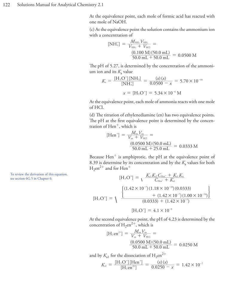
Figure SM9.7 The titration curve for 0.040 M H3PO4 using 0.120 M NaOH as the titrant is shown in blue. The red dashed lines mark volumes of titrant at the equiv-alence points and the red dots marks the first two equivalence points (see Problem 2f ). Note that third equivalence point is not discernible.
0 20 40 60
24
68
1012
14
volume of strong base (mL)
pH
122 Solutions Manual for Analytical Chemistry 2.1
At the equivalence point, each mole of formic acid has reacted with one mole of NaOH.
(c) At the equivalence point the solution contains the ammonium ion with a concentration of
V VM V
501 500
[NH ]
50.0 mL .0 mL(0. 00 M)(50.0 mL) 0.0 M
4NH HCl
NH NH
3
3 3= + =
+ =
+
The pH of 5.27, is determined by the concentration of the ammoni-um ion and its Ka value
.( ) ( ) .K xx x
0 0 10500 5 70[ ][H O ][ ]
NHNH 103
a4
3 #= = - =+
-+
[ ] .x 105 34H O M63 #= =+ -
At the equivalence point, each mole of ammonia reacts with one mole of HCl.
(d) The titration of ethylenediamine (en) has two equivalence points. The pH at the first equivalence point is determined by the concen-tration of Hen+, which is
V VM V
25 3330500 50
[Hen ]
50.0 mL .0 mL(0. M)( .0 mL) 0.0 M
en HCl
en en= + =
+ =
+
Because Hen+ is amphiprotic, the pH at the equivalence point of 8.39 is determine by its concentration and by the Ka values for both H2en2+ and for Hen+
[ ] C KK K C K KH O3
Hen a1
a1 a2 Hen a1 w= +++
+
+
[ ] ( . ) ( . )
( . ) ( . ) ( . )( . ) ( . )
0 0333 1 42 10
1 42 10 1 18 10 0 03331 42 10 1 00 10H O 7
7 10
7 14
3 #
# #
# #=
+++
-
- -
- -) 3
[ ] .4 1 10H O 93 #=+ -
At the second equivalence point, the pH of 4.23 is determined by the concentration of H2en2+, which is
V VM V
0500 5050 250
[H en ]
50.0 mL .0 mL(0. M)( .0 mL) 0.0 M
22
en HCl
en en= + =
+ =
+
and by Ka1 for the dissociation of H2en2+
.( ) ( ) .K xx x
0 0 0 1 42 1025[H en ][H O ][Hen ] 7
a12
23 #= = - =+
+ +-
To review the derivation of this equation, see section 6G.5 in Chapter 6.
123Chapter 9 Titrimetric Methods
[ ] .5 95 10H O 53 #=+ -
At the first equivalence point, each mole of en reacts with one mole of HCl; at the second equivalence point, each mole of en reacts with two moles of HCl.
(e) For citric acid the only discernible equivalence point is the third, which corresponds to the conversion of monohydrogen citrate, HA2–, to citrate, A3–. The concentration of citrate is
V VM V
0 00 5050
4 200
[ ]
50.0 mL .0 mL(0. M)( .0 mL) 0.0 M
AH A HCl
H A H A3
3
3 3= + =
+ =
-
for which
.( ) ( ) .K xx x
0 0200 2 49 10[A ][OH ][HA ] 8
b1 3
2
#= = - =-
- --
[ ] .2 23 10OH 5#=- -
the pOH is 4.65, or a pH of 9.35. At this equivalence point, each mole of citric acid reacts with three moles of NaOH.
(f ) For phosphoric acid, the first and the second equivalence points are the only useful equivalence points. The first equivalence point corresponds to the conversion of H3PO4 to H PO2 4
- and the sec-ond equivalence point corresponds to the conversion of H PO2 4
- to HPO4
2- . The pH at the first equivalence point is determined by the concentration of H PO2 4
- , which is
V VM V[H PO ]
16.7 mL 50.0 mL(0.0400 M)(50.0 mL) 0.0300 M
2 4NaOH H PO
H PO H PO
3 4
3 4 3 4= + =
+=
-
Because H PO2 4- is amphiprotic, the pH of 4.72 is given by
[ ] C KK K C K KH O3
H PO a1
a1 a2 H PO a1 w
2 4
2 4= +++
-
-
[ ] ( . ) ( . )
( ) ( ) ( . )( . ) ( . )
. .
0 03 7 11 10
10 10 0 03007 11 10 1 00 10
00
7 11 6 32
H O 3
3
3 14
8
3 #
# #
# #=
+++
-
-
- -
-
) 3
[ ] . 101 91H O 53 #=+ -
The pH at the second equivalence point is determined by the concen-tration of HPO4
2- , which is
.
V VM V
33 3 240
[HPO ]
mL 50.0 mL(0.0400 M)(50.0 mL) 0.0 M
24
NaOH H PO
H PO H PO
3 4
3 4 3 4= + =
+ =
-
124 Solutions Manual for Analytical Chemistry 2.1
Because HPO42- is amphiprotic, the pH of 9.63 is given by
[ ] C KK K C K KH O
2
3 223
HPO a
a a HPO a w2
2
4
4= +++
-
-
[ ] ( . ) ( . )
( ) ( ) ( . )( . ) ( . )
. .
0 0 6 32 10
10 10 0 06 32 10 1 00 10
240
6 32 4 5 240
H O 8
13
8 14
8
3 #
# #
# #=
+++
-
- -
- -) 3
[ ] . 102 34H O 103 #=+ -
At the first equivalence point, each mole of H3PO4 reacts with one mole of NaOH; at the second equivalence point, each mole of H3PO4 reacts with two moles of NaOH.
3. For each titration curve, an appropriate indicator is determined by comparing the indicator’s pKa and its pH range to the pH at the equivalence point. Using the indicators in Table 9.4, good choices are:
(a) bromothymol blue; (b) cresol red; (c) methyl red; (d) cresol red for the first equivalence point (although the lack of a large change in pH at this equivalence point makes it the less desirable choice) and congo red for the second equivalence point; (e) phenolphthalein; and (f ) bromocresol green for the first equivalence point and phenolphtha-lein for the second equivalence point.
Other indicators from Table 9.4 are acceptable choices as well, pro-vided that the change in color occurs wholly within the sharp rise in pH at the equivalence point.
4. To show that this is the case, let’s assume we are titrating the weak acid HA with NaOH and that we begin with x moles of HA. The reaction between HA and OH– is very favorable, so before the equivalence point we expect that the moles of HA will decrease by an amount equivalent to the moles of OH– added. If we add sufficient OH– to react with 10% of the HA, then the moles of HA that remain is 0.9x. Because we produce a mole of A– for each mole of HA consumed, we have 0.1x moles of A–. From the Henderson-Hasselbalch equation we know that
KpH p log mol HAmol A
a= +-
...K K Kxx 0 950 9
0 1 1pH p log p pa a a.= + = - -
After adding sufficient OH– to consume 90% of the HA, 0.1x moles of HA remain and 0.9x moles of A–; thus
.
. .K xx K K0 1
0 9 0 95 1pH p log p pa a a.= + = + +
5. Tartaric acid is a diprotic weak acid, so our first challenge is to decide which of its two endpoints is best suited for our analysis. As the two
The choice of indicator for (d) illustrates an important point: for a polyprotic weak acid or weak base, you can choose the equivalence point that best meets your needs.
125Chapter 9 Titrimetric Methods
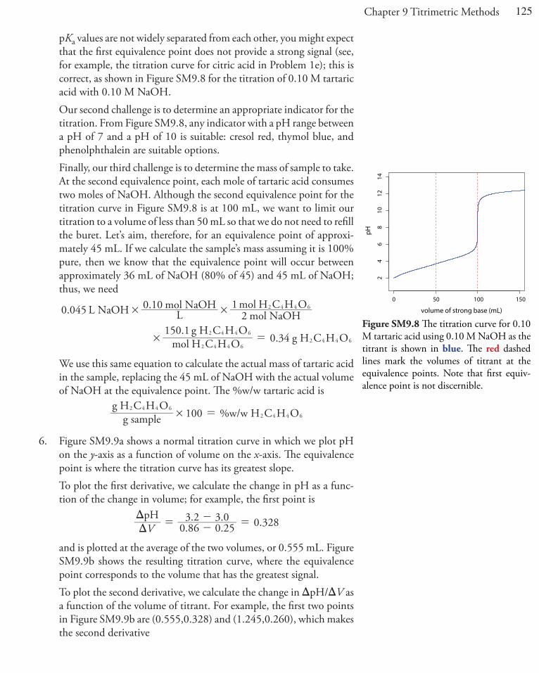
pKa values are not widely separated from each other, you might expect that the first equivalence point does not provide a strong signal (see, for example, the titration curve for citric acid in Problem 1e); this is correct, as shown in Figure SM9.8 for the titration of 0.10 M tartaric acid with 0.10 M NaOH.
Our second challenge is to determine an appropriate indicator for the titration. From Figure SM9.8, any indicator with a pH range between a pH of 7 and a pH of 10 is suitable: cresol red, thymol blue, and phenolphthalein are suitable options.
Finally, our third challenge is to determine the mass of sample to take. At the second equivalence point, each mole of tartaric acid consumes two moles of NaOH. Although the second equivalence point for the titration curve in Figure SM9.8 is at 100 mL, we want to limit our titration to a volume of less than 50 mL so that we do not need to refill the buret. Let’s aim, therefore, for an equivalence point of approxi-mately 45 mL. If we calculate the sample’s mass assuming it is 100% pure, then we know that the equivalence point will occur between approximately 36 mL of NaOH (80% of 45) and 45 mL of NaOH; thus, we need
0.045 L NaOH L0.10 mol NaOH
2 mol NaOH1 mol
mol H C H O150.1 g H C H O
0.34 g H C H O
H C H O
2 4 4 6
2 4 4 62 4 4 6
2 4 4 6# #
# =
We use this same equation to calculate the actual mass of tartaric acid in the sample, replacing the 45 mL of NaOH with the actual volume of NaOH at the equivalence point. The %w/w tartaric acid is
g sampleg H C H O
100 %w/w H C H O2 4 4 62 4 4 6# =
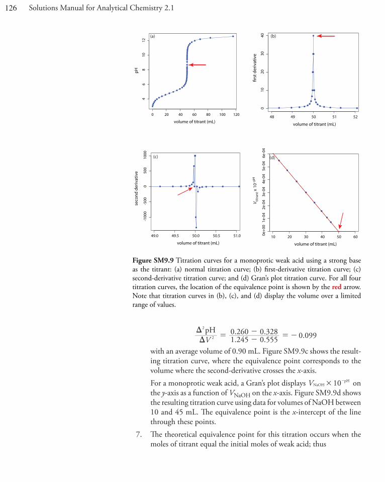
6. Figure SM9.9a shows a normal titration curve in which we plot pH on the y-axis as a function of volume on the x-axis. The equivalence point is where the titration curve has its greatest slope.
To plot the first derivative, we calculate the change in pH as a func-tion of the change in volume; for example, the first point is
. .. . .V 0 86 0 25
3 2 3 0 0 328pHDD
=-- =
and is plotted at the average of the two volumes, or 0.555 mL. Figure SM9.9b shows the resulting titration curve, where the equivalence point corresponds to the volume that has the greatest signal.
To plot the second derivative, we calculate the change in DpH/DV as a function of the volume of titrant. For example, the first two points in Figure SM9.9b are (0.555,0.328) and (1.245,0.260), which makes the second derivative
0 50 100 150
24
68
1012
14
volume of strong base (mL)
pH
Figure SM9.8 The titration curve for 0.10 M tartaric acid using 0.10 M NaOH as the titrant is shown in blue. The red dashed lines mark the volumes of titrant at the equivalence points. Note that first equiv-alence point is not discernible.
126 Solutions Manual for Analytical Chemistry 2.1
. .
. . .V 1 245 0 5550 260 0 328 0 099
pH2
DD
=-- =-2
with an average volume of 0.90 mL. Figure SM9.9c shows the result-ing titration curve, where the equivalence point corresponds to the volume where the second-derivative crosses the x-axis.
For a monoprotic weak acid, a Gran’s plot displays V 10NaOHpH# - on
the y-axis as a function of VNaOH on the x-axis. Figure SM9.9d shows the resulting titration curve using data for volumes of NaOH between 10 and 45 mL. The equivalence point is the x-intercept of the line through these points.
7. The theoretical equivalence point for this titration occurs when the moles of titrant equal the initial moles of weak acid; thus
0 20 40 60 80 100 120
46
810
12
volume of titrant (mL)
pH
(a)
48 49 50 51 52
010
2030
40
volume of titrant (mL)
�rst
der
ivat
ive
(b)
10 20 30 40 50 600e+0
01e
-04
2e-0
43e
-04
4e-0
45e
-04
6e-0
4
volume of titrant (mL)
(d)
V titra
nt x
10–p
H
49.0 49.5 50.0 50.5 51.0
-100
0-5
000
500
1000
volume of titrant (mL)
seco
nd d
eriv
ativ
e
(c)
Figure SM9.9 Titration curves for a monoprotic weak acid using a strong base as the titrant: (a) normal titration curve; (b) first-derivative titration curve; (c) second-derivative titration curve; and (d) Gran’s plot titration curve. For all four titration curves, the location of the equivalence point is shown by the red arrow. Note that titration curves in (b), (c), and (d) display the volume over a limited range of values.
127Chapter 9 Titrimetric Methods
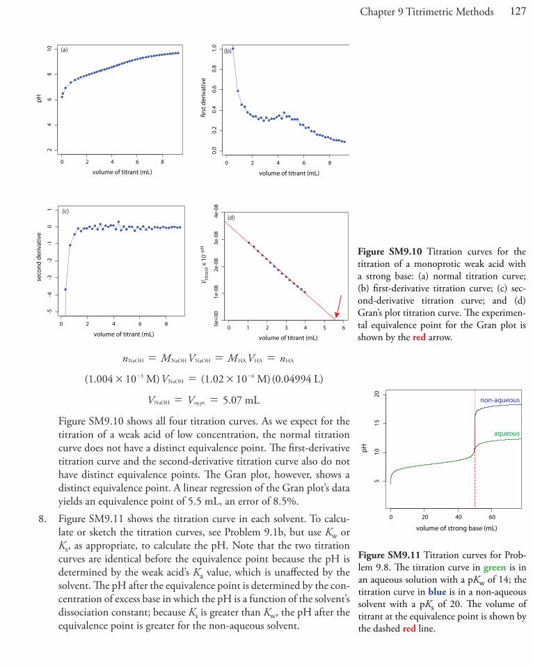
n M V M V nNaOH NaOH NaOH HA HA HA= = =
( . ) ( . ) ( .V1 004 10 1 02 10 0 0M M 4994 L)3 4NaOH# #=- -
V V 5.07 mL. .eq ptNaOH= =
Figure SM9.10 shows all four titration curves. As we expect for the titration of a weak acid of low concentration, the normal titration curve does not have a distinct equivalence point. The first-derivative titration curve and the second-derivative titration curve also do not have distinct equivalence points. The Gran plot, however, shows a distinct equivalence point. A linear regression of the Gran plot’s data yields an equivalence point of 5.5 mL, an error of 8.5%.
8. Figure SM9.11 shows the titration curve in each solvent. To calcu-late or sketch the titration curves, see Problem 9.1b, but use Kw or Ks, as appropriate, to calculate the pH. Note that the two titration curves are identical before the equivalence point because the pH is determined by the weak acid’s Ka value, which is unaffected by the solvent. The pH after the equivalence point is determined by the con-centration of excess base in which the pH is a function of the solvent’s dissociation constant; because Ks is greater than Kw, the pH after the equivalence point is greater for the non-aqueous solvent.
Figure SM9.10 Titration curves for the titration of a monoprotic weak acid with a strong base: (a) normal titration curve; (b) first-derivative titration curve; (c) sec-ond-derivative titration curve; and (d) Gran’s plot titration curve. The experimen-tal equivalence point for the Gran plot is shown by the red arrow.
Figure SM9.11 Titration curves for Prob-lem 9.8. The titration curve in green is in an aqueous solution with a pKw of 14; the titration curve in blue is in a non-aqueous solvent with a pKs of 20. The volume of titrant at the equivalence point is shown by the dashed red line.
0 2 4 6 8
24
68
10
volume of titrant (mL)
pH
(a)
0 2 4 6 8
0.0
0.2
0.4
0.6
0.8
1.0
volume of titrant (mL)
�rst
der
ivat
ive
(b)
0 2 4 6 8
-5-4
-3-2
-10
1
volume of titrant (mL)
seco
nd d
eriv
ativ
e
(c)
0 1 2 3 4 5 60e+0
01e
-08
2e-0
83e
-08
4e-0
8
volume of titrant (mL)
V titra
nt x
10–p
H
(d)
0 20 40 60
510
1520
volume of strong base (mL)
pH
non-aqueous
aqueous

128 Solutions Manual for Analytical Chemistry 2.1
9. This is an interesting example of a situation where we cannot use a visual indicator. As we see in Figure SM9.12, because the two analytes have pKa values that are not sufficiently different from each other, the potentiometric titration curve for o-nitrophenol does not show a discernible equivalence point.
For the spectrophotometric titration curve, the corrected absorbance increases from the first addition of NaOH as o-nitrophenol reacts to form o-nitrophenolate. After the first equivalence point we begin to convert m-nitrophenol to m-nitrophenolate; the rate of change in the corrected absorbance increases because m-nitrophenolate ab-sorbs light more strongly than does o-nitrophenolate. After the sec-ond equivalence point, the corrected absorbance remains constant because there is no further increase the amounts of o-nitrophenolate or of m-nitrophenolate.
10. (a) With a Kb of 3.94×10⁻¹⁰, aniline is too weak of a base to titrate easily in water. In an acidic solvent, such as glacial acetic acid, aniline behaves as a stronger base.
(b) At a higher temperature, the molar concentration of HClO4 de-creases because the moles of HClO4 remain unchanged but the vol-ume of solution is larger. Titrating the solution of aniline at 27°C, therefore, requires a volume of titrant that is greater than when we complete the titration at 25°C. As a result, we overestimate the moles of HClO4 needed to reach the equivalence point and report a con-centration of HClO4 that is too large.
(c) A sample that contains 3-4 mmol of aniline will require
. . .V 0 10003 4 10 0 030 0 040M
– mol aniline L–3
HClO4
#= =-
30–40 mL of HClO4 to reach the equivalence point. If we take a sam-ple with significantly more aniline, we run the risk of needing more than 50 mL of titrant. This requires that we stop the titration and refill the buret, introducing additional uncertainty into the analysis.
11. Figure SM9.13 shows the ladder diagram for H2CO3. When we stan-dardize a solution of NaOH we must ensure that the pH at the end-point is below 6 so that dissolved CO2, which is present as H2CO3, does not react with NaOH. If the endpoint’s pH is between 6 and 10, then NaOH reacts with H2CO3, converting it to HCO3
- ; as a result, we overestimate the volume of NaOH that reacts with our primary standard and underestimate the titrant’s concentration.
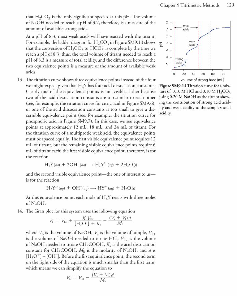
12. Figure SM9.14 shows the full titration curve, although our focus in this problem is on the first two equivalence points. At the titration’s first equivalence point, the pH is sufficiently acidic that a reaction is unlikely between NaOH and any weak acids in the sample. The ladder diagram for H2CO3 in Figure SM9.13, for example, shows
0 20 40 60
24
68
1012
14
volume of strong base (mL)
pH
corrected absorbance
Figure SM9.12 Titration curves for Prob-lem 9.9 with the volume of titrant at the equivalence points shown by the dashed red lines. The potentiometric titration curve is shown in blue. Of the two equivalence points, only the second—for m-nitrophe-nol—is discernible. The spectrophotomet-ric titration curve, which is shown by the green line, has a distinct equivalence point for each analyte.
pKa = 6.352
pKa = 10.329
pH
H2CO3
HCO3–
CO32–
Figure SM9.13 Ladder diagram for H2CO3.
129Chapter 9 Titrimetric Methods
that H2CO3 is the only significant species at this pH. The volume of NaOH needed to reach a pH of 3.7, therefore, is a measure of the amount of available strong acids.
At a pH of 8.3, most weak acids will have reacted with the titrant. For example, the ladder diagram for H2CO3 in Figure SM9.13 shows that the conversion of H2CO3 to HCO3
- is complete by the time we reach a pH of 8.3; thus, the total volume of titrant needed to reach a pH of 8.3 is a measure of total acidity, and the difference between the two equivalence points is a measure of the amount of available weak acids.
13. The titration curve shows three equivalence points instead of the four we might expect given that H4Y has four acid dissociation constants. Clearly one of the equivalence points is not visible, either because two of the acid dissociation constants are too similar to each other (see, for example, the titration curve for citric acid in Figure SM9.6), or one of the acid dissociation constants is too small to give a dis-cernible equivalence point (see, for example, the titration curve for phosphoric acid in Figure SM9.7). In this case, we see equivalence points at approximately 12 mL, 18 mL, and 24 mL of titrant. For the titration curve of a multiprotic weak acid, the equivalence points must be spaced equally. The first visible equivalence point requires 12 mL of titrant, but the remaining visible equivalence points require 6 mL of titrant each; the first visible equivalence point, therefore, is for the reaction
( ) ( ) ( ) ( )aq aq aq lH Y 2OH H Y 2H O24 2 2$+ +- -
and the second visible equivalence point—the one of interest to us—is for the reaction
( ) ( ) ( ) ( )aq aq aq lH Y OH HY H O2 32 2$+ +- - -
At this equivalence point, each mole of H4Y reacts with three moles of NaOH.
14. The Gran plot for this system uses the following equation
[ ]( )V V K
K VM
V V dH Ob E1
3 a
a E2
b
a b= +
+-
++
where Vb is the volume of NaOH, Va is the volume of sample, VE1 is the volume of NaOH needed to titrate HCl, VE2 is the volume of NaOH needed to titrate CH3COOH, Ka is the acid dissociation constant for CH3COOH, Mb is the molarity of NaOH, and d is [H3O+] – [OH–]. Before the first equivalence point, the second term on the right side of the equation is much smaller than the first term, which means we can simplify the equation to
( )V V MV V d
b E1b
a b= -
+
0 20 40 60 80 100
24
68
1012
14
volume of strong base (mL)
pH
strongacids
weakacids
totalacids
Figure SM9.14 Titration curve for a mix-ture of 0.10 M HCl and 0.10 M H2CO3 using 0.20 M NaOH as the titrant show-ing the contribution of strong acid acid-ity and weak acidity to the sample’s total acidity.
130 Solutions Manual for Analytical Chemistry 2.1
and a plot of Vb versus (Va + Vb)d is a straight-line with a y-intercept of VE1. After the second equivalence point, the [H3O+] is much smaller than Ka and the full Gran plot equation reduces to
( )V V V MV V d
b E1 E2b
a b= + -
+
and a plot of Vb versus (Va + Vb)d is a straight-line with a y-intercept of VE1 + VE2.
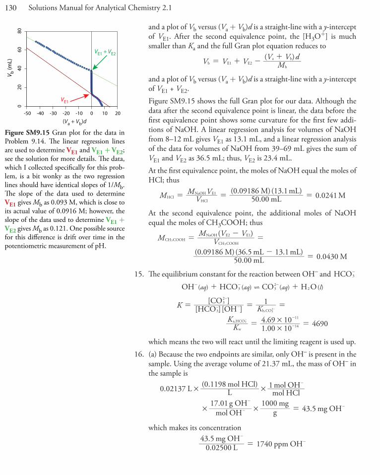
Figure SM9.15 shows the full Gran plot for our data. Although the data after the second equivalence point is linear, the data before the first equivalence point shows some curvature for the first few addi-tions of NaOH. A linear regression analysis for volumes of NaOH from 8–12 mL gives VE1 as 13.1 mL, and a linear regression analysis of the data for volumes of NaOH from 39–69 mL gives the sum of VE1 and VE2 as 36.5 mL; thus, VE2 is 23.4 mL.
At the first equivalence point, the moles of NaOH equal the moles of HCl; thus
M VM V
50.00 mL(0.09186 M)(13.1 mL) 0.0241 MHCl
HCl
NaOH E1= = =
At the second equivalence point, the additional moles of NaOH equal the moles of CH3COOH; thus
( )M VM V V
43050.00 mL(0.09186 M)(36.5 mL 13.1 mL) 0.0 M
CH COOH
NaOH E2 E1CH COOH
33 =
-=
-=
15. The equilibrium constant for the reaction between OH– and HCO3-
( ) ( ) ( ) ( )aq aq aq lOH HCO CO H O3 32
2?+ +- - -
.
.
K K
KK
1
1 00 104 69 10 4690
[HCO ][OH ][CO ]
14
11
3–
32
b,CO
w
a,HCO
32
3
##
= = =
= =
-
-
-
-
-
-
which means the two will react until the limiting reagent is used up.16. (a) Because the two endpoints are similar, only OH– is present in the
sample. Using the average volume of 21.37 mL, the mass of OH– in the sample is
0.02137 L L(0.1198 mol HCl)
mol HCl1 mol OH
mol OH17.01 g OH
g1000 mg
43.5 mg OH
# #
# # =
-
-
-
-
which makes its concentration
0.02500 L43.5 mg OH
1740 ppm OH=-
-
-50 -40 -30 -20 -10 0 10 20
020
4060
80
V b (mL)
(Va + Vb)d
VE1
VE1 + VE2
Figure SM9.15 Gran plot for the data in Problem 9.14. The linear regression lines are used to determine VE1 and VE1 + VE2; see the solution for more details. The data, which I collected specifically for this prob-lem, is a bit wonky as the two regression lines should have identical slopes of 1/Mb. The slope of the data used to determine VE1 gives Mb as 0.093 M, which is close to its actual value of 0.0916 M; however, the slope of the data used to determine VE1 + VE2 gives Mb as 0.121. One possible source for this difference is drift over time in the potentiometric measurement of pH.
131Chapter 9 Titrimetric Methods
(b) Because the volume to reach the bromocresol green end point is more than twice that to reach the phenolphthalein end point, the sample must contain a mixture of CO3
2- and HCO3- . Only CO3
2- is neutralized when we titrate to the phenolphthalein end point, form-ing HCO3
- as a product; thus
..
60 01
056
0 8
0.0 7 L L(0.1198 mol HCl)
mol HCl1 mol
mol COg CO
g1000 mg
4 mg CO
CO
32
32
32
32
# #
# # =-
-
-
-
0.02500 L40.8 mg CO
1630 ppm CO32
32=
-
-
We know that it takes 5.67 mL of HCl to titrate CO32- to HCO3
- , which means it takes 2 × 5.67 mL, or 11.34 mL of HCl to reach the second end point for CO3
2- . The volume of HCl used to titrate HCO3
- is 21.13 mL – 11.34 mL, or 9.79 mL; thus, the concentration of HCO3
- in the sample is
..
0
6 0
979
1 271 6
0.0 L L(0.1198 mol HCl)
mol HCl1 mol HCO
mol HCOg HCO
g1000 mg
mg HCO
3
3
33
# #
# # =
-
-
-
-
.286
71 60.02500 L
mg HCO0 ppm HCO3
3=-
-
(c) A sample that requires no HCl to reach the phenolphthalein end point contains HCO3
- only; thus, the concentration of HCO3- in the
sample is
..
61 02
1428
104 4
0.0 L L(0.1198 mol HCl)
mol HCl1 mol HCO
mol HCOg HCO
g1000 mg
mg HCO
3
3
33
# #
# # =
-
-
-
-
.4180
104 40.02500 L
mg HCOppm HCO3
3=-
-
(d) If the volume to reach the bromocresol end point is twice that to reach the phenolphthalein end point, then the sample contains CO3
2- only; thus, using the volume of HCl used to reach the phenolphtha-lein end point, we find that the concentration of CO3
2- is
..
60 01123 1
17120.0 L L(0.1198 mol HCl)
mol HCl1 mol CO
mol COg CO
g1000 mg
mg CO
32
32
32
32
# #
# # =
-
-
-
-
.123 149200.02500 L
mg COppm CO3
2
32=
-
-
We can use the volume to reach the bro-mocresol green end point as well, substi-tuting
2 mol HCl1 mol CO3
2-
for
1 mol HCl1 mol CO3
2-
132 Solutions Manual for Analytical Chemistry 2.1
(e) If the volume to reach the bromocresol green end point is less than twice the volume to reach the phenolphthalein end point, then we know the sample contains CO3
2- and OH–. Because OH– is neutral-ized completely at the phenolphthalein end point, the difference of 4.33 mL in the volumes between the two end points is the volume of HCl used to titrate CO3
2- ; thus, its concentration is
..
0
60 01
433
31 1
0.0 L L(0.1198 mol HCl)
mol HCl1 mol CO
mol COg CO
g1000 mg
mg CO
32
32
32
32
# #
# # =
-
-
-
-
.31 12400.02500 L
mg CO1 ppm CO3
2
32=
-
-
At the phenolphthalein end point, the volume of HCl used to neu-tralize OH– is the difference between the total volume, 21.36 mL, and the volume used to neutralize CO3
2- , 4.33 mL, or 17.03 mL; thus, its concentration is
.
1703
34 7
0.0 L L(0.1198 mol HCl)
mol HCl1 mol OH
mol OH17.01 g OH
g1000 mg
mg OH
# #
# # =
-
-
-
-
.34 73900.02500 L
mg OH1 ppm OH=
-
-
17. (a) When using HCl as a titrant, a sample for which the volume to reach the methyl orange end point is more than twice the volume to reach the phenolphthalein end point is a mixture of HPO4
2- and PO4
3- . The titration to the phenolphthalein end point involves PO43-
only; thus, its concentration is.M V
M V 11 54 5325.00 mL(0.1198 M)( mL) 0.05 MPO
sample
HCl HCl43 = = =-
We know that it takes 11.54 mL of HCl to titrate PO43- to HPO4
2- , which means it takes 2 × 11.54 mL, or 23.08 mL of HCl to reach the second end point for PO4
3- . The volume of HCl used to titrate HPO4
2- is 35.29 mL – 23.08 mL, or 12.21 mL; thus, the concentra-tion of HPO4
2- in the sample is.M V
M V 12 21 8525.00 mL(0.1198 M)( mL) 0.05 MHPO
sample
HCl HCl43 = = =-
(b) When using NaOH as the titrant, a sample for which the volume to reach the phenolphthalein end point is twice the volume to reach the methyl orange end point contains H3PO4 only; thus, the concen-tration of H3PO4 is
. .M VM V 9 89 0 047425.00 mL
(0.1198 M)( mL) MH POsample
NaOH NaOH3 4 = = =
133Chapter 9 Titrimetric Methods
(c) When using HCl as a titrant, a sample that requires identical vol-umes to reach the methyl orange and the phenolphthalein end points contains OH– only; thus, the concentration of OH– is
..M VM V 022 77 109125.00 mL
(0.1198 M)( mL) Msample
OHHCl HCl= = =-
(d) When using NaOH as the titrant, a sample for which the volume to reach the phenolphthalein end point is more than twice the volume to reach the methyl orange end point contains a mixture of H3PO4 and H PO2 4
- . The titration to the methyl orange end point involves H3PO4 only; thus, its concentration is
..M VM V 0 017 48 83825.00 mL
(0.1198 M)( mL) MH POsample
NaOH NaOH3 4 = = =
We know that it takes 17.48 mL of NaOH to titrate H3PO4 to H PO2 4
- , which means it takes 2 × 17.48 mL, or 34.96 mL of NaOH to reach the second end point for H3PO4. The volume of NaOH used to titrate H PO2 4
- is 39.42 mL – 34.96 mL, or 4.46 mL; thus, the concentration of H PO2 4
- in the sample is
..M VM V 0 04 46 21425.00 mL
(0.1198 M)( mL) MH POsample
NaOH NaOH42 = = =-
18. For this back titration, the moles of HCl must equal the combined moles of NH3 and of NaOH; thus
n n n M V M VNH HCl NaOH HCl HCl NaOH NaOH3 = - = -
.n
n 2 509 10(0.09552 M)(0.05000 L) (0.05992 M)(0.03784 L)
mol NHNH
NH3
3
3
3 #
= -
= -
2.509 10 mol NH mol NH14.007 g N
0.03514 g N33
3# # =-
0.03514 g N 0.1754 g N1 g protein
0.2003 g protein# =
1.2846 g sample0.2003 g protein
100 15.59% w/w protein# =
19. The sulfur in SO2 is converted to H2SO4, and titrated with NaOH to the phenolphthalein end point, converting H2SO4 to SO4
2- and consuming two moles of NaOH per mole of H2SO4; thus, there are
0.01008 L L0.0244 mol NaOH
2 mol NaOH1 mol H SO
mol H SO1 mol SO
mol SO64.06 g SO
g1000 mg
7.88 mg SO
2 4
2 4
2
2
22
# #
# # # =
in the sample. The volume of air sampled is 1.25 L/min × 60 min, or 75.0 L, which leaves us with an SO2 concentration of
134 Solutions Manual for Analytical Chemistry 2.1
75.0 L
7.78 mg SO 2.86 mg SO1 mL
mL1000 µL
36.7 µL/L SO2
22
# #=
20. We begin the analysis with
L0.0200 mol Ba(OH) 0.05000 L 1.00 10 mol Ba(OH)2 3
2# #= -
The titration of Ba(OH)2 by HCl consumes two moles of HCl for every mole of Ba(OH)2; thus,
0.03858 mL L0.0316 M HCl
2 mol HCl1 mol Ba(OH) 6.10 10 mol Ba(OH)2 4
2
# #
#= -
react with HCl, leaving
1.00 10 mol Ba(OH) 6.10 10 mol Ba(OH)32
42# #-- -
or 3.90×10⁻⁴ mol Ba(OH)2 to react with CO2. Because each mole of CO2 reacts with one mole of Ba(OH)2 to form BaCO3, we know that the sample of air has 3.90×10⁻⁴ mol CO2; thus, the concentration of CO2 is
163.90 10 mol CO mol CO44.01 g CO
0.017 g CO42
2
22# # =-
6
3.5 L
0.0171 g CO 1.98 g CO1 L CO
L10 µL
2480 µL/L CO2
2
26
2
# #=
21. From the reaction in Table 9.8, we see that each mole of methylethyl ketone, C4H8O, releases one mole of HCl; thus, the moles of NaOH used in the titration is equal to the moles of C4H8O in the sample. The sample’s purity, therefore, is
0.03268 mL L0.9989 mol NaOH
mol NaOH1 mol C H O
mol C H O72.11 g C H O
2.354 g C H O8
4 8
4 84 8
4
# #
# =
3.00 mL sample
2.354 g C H O 0.805 g1 mL
100 97.47%4 8 #
# =
22. For this back titration, the total moles of KOH used is equal to the moles that react with HCl in the titration and the moles that react with the butter. The total moles of KOH is
0.02500 L L0.5131 mol KOH 0.01283 mol KOH# =
and the moles of KOH that react with HCl is
135Chapter 9 Titrimetric Methods
.0 00513
0.01026 L L0.5000 mol HCl
mol HCl1 mol KOH mol KOH
# #
=
which means that 0.01283 mol KOH 0.00513 mol KOH
mol KOH56.10 g KOH
g1000 mg
432.0 mg KOH
#
#
-
=
^ h
react with the butter. The saponification number for butter is
2.085 g butter432.0 mg KOH
207=
23. To calculate the weak acid’s equivalent weight, we treat the titration reaction as if each mole of weak acid reacts with one mole of strong base; thus, the weak acid’s equivalent weight is
0
0
0. 3258 L L0.0556 mol NaOH
mol NaOH1 mol acid 0.0 1811 mol acid
# #
=
0.001811 mol acid0.2500 g acid
138 g/mol=
24. To identify the amino acid, we use the titration curve to determine its equivalent weight and its Ka value. The titration’s equivalence point is approximately 34 mL. The pH at half this volume provides an es-timate of the amino acid’s pKa; this is approximately 8.6, or a Ka of 2.5 × 10⁻⁹. From the list of possible amino acids, taurine and aspar-agine are likely candidates.
Using our estimate of 34 mL for the equivalence point, the amino acid’s equivalent weight is
0 1036
0
34
352
0. L L0. mol NaOH
mol NaOH1 mol acid 0.0 mol acid
# #
=
3524300
1200.00 mol acid0. g acid
g/mol=
As this is closer to the formula weight of taurine than of asparagine, taurine is the most likely choice for the amino acid.
25. From Figure SM9.9, we see that the equivalence point is at 50.0 mL of NaOH. The pH at half this volume is approximately 4.8, which makes the pKa 4.8 and the Ka value 1.6 × 10⁻⁵.
26. The method illustrated in Figure 9.24 uses a sample of approximately 20 µL; if we assume a density of 1 g/mL, this is equivalent to a sam-ple that weighs 20 mg, or a meso sample. The method illustrated in
A density of 1 g/ml is the same as 1 mg/µL; thus, a 20 µL sample weighs 20 mg.
136 Solutions Manual for Analytical Chemistry 2.1
Figure 9.27 uses an approximately 1 pL sample; if we assume a den-sity of 1 g/mL, this corresponds to a sample that weight 1 ng, or an ultramicro sample. For both methods, the need to see the titration’s visual end point requires a major or, perhaps, a minor analyte.
27. To determine an analyte’s formula weight requires that we know the stoichiometry between the analyte and the titrant. Even if a titration curve shows a single equivalence point, we cannot be sure if it rep-resents the titration of a single proton or if it represents the titration of two or more protons that are too similar in their acid-base strength. To calculate the equivalent weight we simply assume that for any equivalence point, one mole of acid reacts with one mole of base.
28. An titration is designed to use most of the buret’s volume without exceeding its maximum volume. The latter point is important because refilling the buret introduces additional uncertainty. Because the pro-cedure is designed for a sample that is 30–40%w/w Na2CO3, using the procedure for a sample that is more than 98%w/w Na2CO3 will require approximately 2.5–3.3×more titrant. To reduce the amount of titrant we can do one or more of the following: we can reduce the sample’s mass; we can dissolve the sample of washing soda in a larger volume of water; we can take a smaller portion of the dissolved sam-ple; or we can increase the concentration of NaOH.
29. (a) Systematic error. Because the actual mass of KHP is greater than we think, by 0.15 g, we report a concentration for NaOH that is smaller than its actual concentration.
(b) Systematic error. Because KHP is a weak acid, the actual equiv-alence point for its titration is at a pH that is greater than 7. If the indicator signals the end point when the pH is between 3 and 4, we will use less NaOH than expected, which means we will report a concentration for NaOH that is greater than its actual concentration.
(c) Systematic error. The loss of an air bubble in the buret’s tip means that the volume of NaOH in the buret decreases without actually adding NaOH to the solution of KHP. The effect is to increase the apparent volume of NaOH, which means we report a concentration that is smaller than its actual value.
(d) Random error. Because each flask has a different mass, some of our flasks will weigh more than the flask we used to tare the balance; other flasks, of course, will weigh less.
(e) Systematic error. The reason we dry the KHP is to ensure it is free from moisture so that we can calculate the moles of KHP from its mass. Because the reported mass of KHP is too large, we report a concentration of NaOH that is greater than its actual concentration.
Look back, for example, at the titration curve for citric acid in Figure SM9.6 in which the single equivalence point occurs when each mole of citric acid has reacted with three moles of NaOH.
A density of 1 g/mL is equivalent to 1 ng/pL; thus, a 1 pL sample weighs 1 ng.
The change in volume of NaOH in the buret is equivalent to the volume of the air bubble.
137Chapter 9 Titrimetric Methods
(f ) No affect on error. We do not use the mass of NaOH in our calcu-lations; thus, any uncertainty in its mass has no effect on our results.
(g) No affect on error. The volume of water used to dissolve the KHP is not used to calculate the concentration of NaOH.
30. (a) If we carry out the titration too quickly, we may neutralize the ex-tracted o-phthalic acid—triggering the end point’s signal—and stop the titration long before the remaining o-phthalic acid has time to extract. As a result, we underestimate the concentration of o-phthalic acid.
(b) If we wish to carry out the titration more quickly, we can add an excess of NaOH to the sample, allow time for the o-phthalic acid to extract into the NaOH and react, and then back-titrate the excess NaOH using a strong acid.
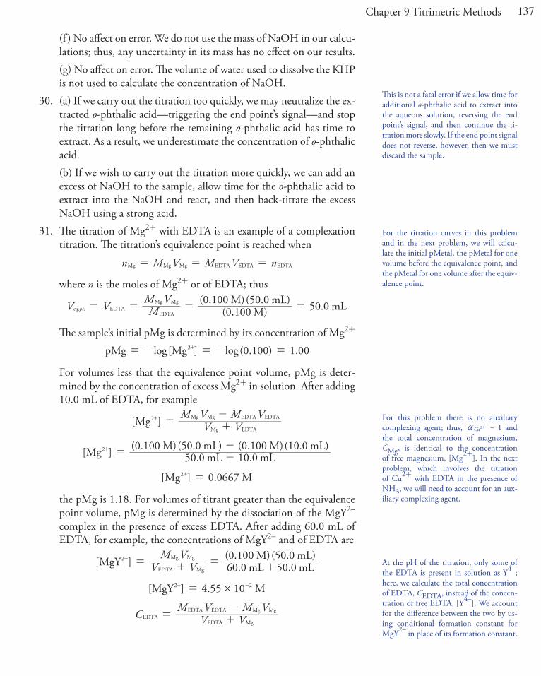
31. The titration of Mg2+ with EDTA is an example of a complexation titration. The titration’s equivalence point is reached when
n M V M V nMg Mg Mg EDTA EDTA EDTA= = =
where n is the moles of Mg2+ or of EDTA; thus
V V MM V
(0.100 M)(0.100 M)(50.0 mL) 50.0 mL. .eq pt EDTA
EDTA
Mg Mg= = = =
The sample’s initial pMg is determined by its concentration of Mg2+
( . ) .log 0 1 00100pMg log[Mg ]2=- =- =+
For volumes less that the equivalence point volume, pMg is deter-mined by the concentration of excess Mg2+ in solution. After adding 10.0 mL of EDTA, for example
[ V VM V M VMg ]2
Mg EDTA
Mg Mg EDTA EDTA= +
-+
[Mg ] 50.0 mL 10.0 mL(0.100 M)(50.0 mL) (0.100 M)(10.0 mL)2 = +
-+
[Mg ] 0.0667 M2 =+
the pMg is 1.18. For volumes of titrant greater than the equivalence point volume, pMg is determined by the dissociation of the MgY2– complex in the presence of excess EDTA. After adding 60.0 mL of EDTA, for example, the concentrations of MgY2– and of EDTA are
] V VM V[MgY 60.0 mL 50.0 mL
(0.100 M)(50.0 mL)2
EDTA Mg
Mg Mg= + =
+-
][MgY 4.55 10 M2 2#=- -
V VM V M VC
EDTA Mg
EDTA EDTA Mg MgEDTA = +
-
For this problem there is no auxiliary complexing agent; thus, Cd2a + = 1 and the total concentration of magnesium, CMg, is identical to the concentration of free magnesium, [Mg2+]. In the next problem, which involves the titration of Cu2+ with EDTA in the presence of NH3, we will need to account for an aux-iliary complexing agent.
At the pH of the titration, only some of the EDTA is present in solution as Y4–; here, we calculate the total concentration of EDTA, CEDTA, instead of the concen-tration of free EDTA, [Y4–]. We account for the difference between the two by us-ing conditional formation constant for MgY2– in place of its formation constant.
This is not a fatal error if we allow time for additional o-phthalic acid to extract into the aqueous solution, reversing the end point’s signal, and then continue the ti-tration more slowly. If the end point signal does not reverse, however, then we must discard the sample.
For the titration curves in this problem and in the next problem, we will calcu-late the initial pMetal, the pMetal for one volume before the equivalence point, and the pMetal for one volume after the equiv-alence point.
138 Solutions Manual for Analytical Chemistry 2.1
C 60.0 mL 50.0 mL(0.100 M)(60.0 mL) (0.100 M)(50.0 mL)
EDTA = +-
.C 9 09 10 M3EDTA #= -
For a pH of 10, substituting these concentrations into the conditional formation constant for MgY2– and solving for [Mg2+]
]] ( . ) ( . ) .C K 6 2 10 0 367 2 3 10
[MgY[Mg f
2
28 8
EDTAY4 # #a= = =
-
+ -
] .( . ). 2 3 109 09 10
4 55 10[Mg2
83
2
##
# =+ -
-
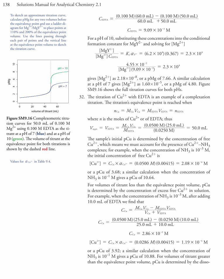
gives [Mg2+] as 2.18×10⁻⁸, or a pMg of 7.66. A similar calculation at a pH of 7 gives [Mg2+] as 1.60×10⁻⁵, or a pMg of 4.80. Figure SM9.16 shows the full titration curves for both pHs.
32. The titration of Cu2+ with EDTA is an example of a complexation titration. The titration’s equivalence point is reached when
n M V M V nCu Cu EDTA EDTA EDTACu= = =
where n is the moles of Cu2+ or of EDTA; thus
V V MM V
025050 25
(0. 0 M)(0. 0 M)( .0 mL) 50.0 mL. .eq pt EDTA
EDTA
Cu Cu= = = =
The sample’s initial pCu is determined by the concentration of free Cu2+, which means we must account for the presence of Cu2+–NH3 complexes; for example, when the concentration of NH3 is 10–3 M, the initial concentration of free Cu2+ is
] ( . ) ( . ) .MC 0 0500 0 00415 2 08 10[Cu M2 4Cu Cu2# #a= = =+ -
+
or a pCu of 3.68; a similar calculation when the concentration of NH3 is 10–1 M gives a pCu of 10.64.
For volumes of titrant less than the equivalence point volume, pCu is determined by the concentration of excess free Cu2+ in solution. For example, when the concentration of NH3 is 10–3 M, after adding 10.0 mL of EDTA we find that
C V VM V M V
CuCu EDTA
Cu Cu EDTA EDTA= +-
C 25.0 mL 10.0 mL(0.0500 M)(25.0 mL) (0.0250 M)(10.0 mL)
Cu= +-
.C 2 86 10 M2Cu #= -
] ( . ) ( . ) .C M0 0 0 00415 10286 1 19[Cu M2 4Cu Cu2# #a= = =+ -
+
or a pCu of 3.92; a similar calculation when the concentration of NH3 is 10–1 M gives a pCu of 10.88. For volumes of titrant greater than the equivalence point volume, pCu is determined by the disso-
0 20 40 60
02
46
810
volume of titrant (mL)
pMg
pH = 7
pH = 10
Figure SM9.16 Complexometric titra-tion curves for 50.0 mL of 0.100 M Mg2+ using 0.100 M EDTA as the ti-trant at a pH of 7 (blue) and at a pH of 10 (green). The volume of titrant at the equivalence point for both titrations is shown by the dashed red line.
To sketch an approximate titration curve, calculate pMg for any two volumes before the equivalence point and use a ladder di-agram for Mg2+/MgY2– to place points at 110% and 200% of the equivalence point volume. Use the lines passing through each pair of points and the vertical line at the equivalence point volume to sketch the titration curve.
Values for Cu2a + in Table 9.4.
139Chapter 9 Titrimetric Methods
ciation of the CuY2– complex in the presence of excess EDTA. After adding 60.0 mL of EDTA, for example, the concentrations of CuY2– and of EDTA are
] V VM V
2505 0 25[CuY 60.0 mL .0 mL
(0. 0 M)( .0 mL)2
EDTA Cu
Cu Cu= + =+
-
] .1 47[CuY 10 M2 2#=- -
C V VM V M V
EDTAEDTA Cu
EDTA EDTA CuCu= +-
C 05025
0250 2560.0 mL .0 mL
(0. M)(60.0 mL) (0. 0 M)( .0 mL)EDTA = +
-
.C 2 94 10 M3EDTA #= -
For a pH of 10, substituting these concentrations into the conditional formation constant for CuY2– and solving for [Cu2+]
]
( . ) ( . ) ( . ) .C C K
6 3 10 0 00415 0 367 9 6 10
[CuYf Cu
2
18 15Cu EDTA
Y2 4
# #
a a= =
=
-
+ -
( . ). .C 2 94 10
1 47 10 9 6 103
215
Cu ## #=-
-
.C 5 0 10 M16Cu #= -
]( . ) ( . ) .
CM5 00 10 0 00415 2 1 10
[CuM
2
16 18
Cu Cu2#
# #
a= =
=
+
- -
+
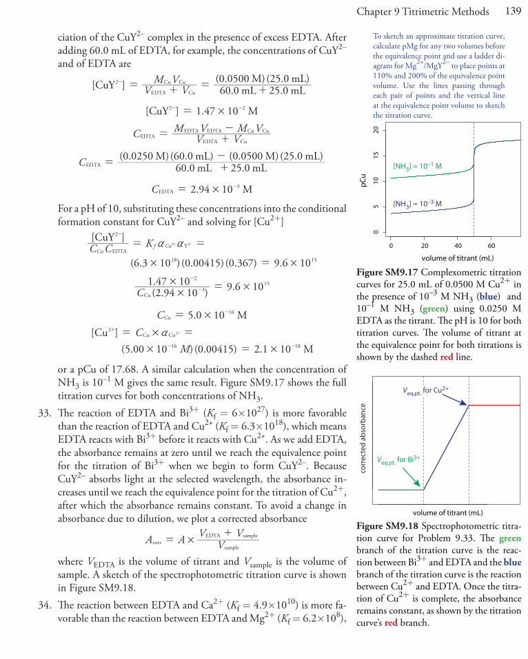
or a pCu of 17.68. A similar calculation when the concentration of NH3 is 10–1 M gives the same result. Figure SM9.17 shows the full titration curves for both concentrations of NH3.
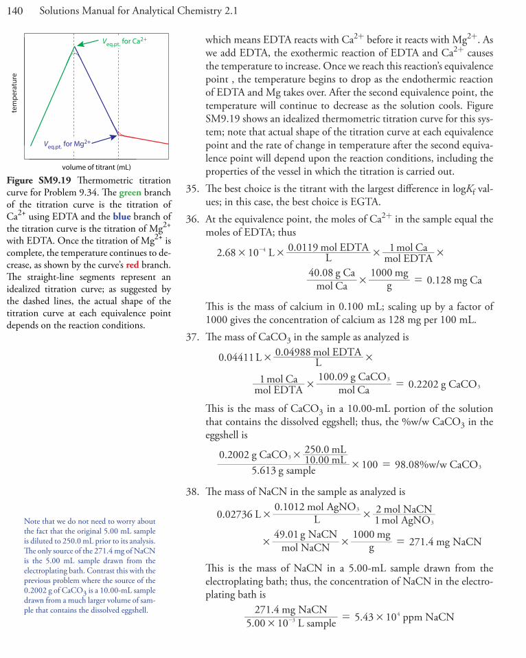
33. The reaction of EDTA and Bi3+ (Kf = 6×1027) is more favorable than the reaction of EDTA and Cu2+ (Kf = 6.3×10¹⁸), which means EDTA reacts with Bi3+ before it reacts with Cu2+. As we add EDTA, the absorbance remains at zero until we reach the equivalence point for the titration of Bi3+ when we begin to form CuY2–. Because CuY2– absorbs light at the selected wavelength, the absorbance in-creases until we reach the equivalence point for the titration of Cu2+, after which the absorbance remains constant. To avoid a change in absorbance due to dilution, we plot a corrected absorbance
A A VV V
corrsample
EDTA sample#=
+
where VEDTA is the volume of titrant and Vsample is the volume of sample. A sketch of the spectrophotometric titration curve is shown in Figure SM9.18.
34. The reaction between EDTA and Ca2+ (Kf = 4.9×10¹⁰) is more fa-vorable than the reaction between EDTA and Mg2+ (Kf = 6.2×10⁸),
Figure SM9.17 Complexometric titration curves for 25.0 mL of 0.0500 M Cu2+ in the presence of 10–3 M NH3 (blue) and 10–1 M NH3 (green) using 0.0250 M EDTA as the titrant. The pH is 10 for both titration curves. The volume of titrant at the equivalence point for both titrations is shown by the dashed red line.
To sketch an approximate titration curve, calculate pMg for any two volumes before the equivalence point and use a ladder di-agram for Mg2+/MgY2– to place points at 110% and 200% of the equivalence point volume. Use the lines passing through each pair of points and the vertical line at the equivalence point volume to sketch the titration curve.
0 20 40 60
05
1015
20
volume of titrant (mL)
pCu
[NH3] = 10–1 M
[NH3] = 10–3 M
volume of titrant (mL)
corr
ecte
d ab
sorb
ance
Veq.pt. for Bi3+
Veq.pt. for Cu2+
Figure SM9.18 Spectrophotometric titra-tion curve for Problem 9.33. The green branch of the titration curve is the reac-tion between Bi3+ and EDTA and the blue branch of the titration curve is the reaction between Cu2+ and EDTA. Once the titra-tion of Cu2+ is complete, the absorbance remains constant, as shown by the titration curve’s red branch.
140 Solutions Manual for Analytical Chemistry 2.1
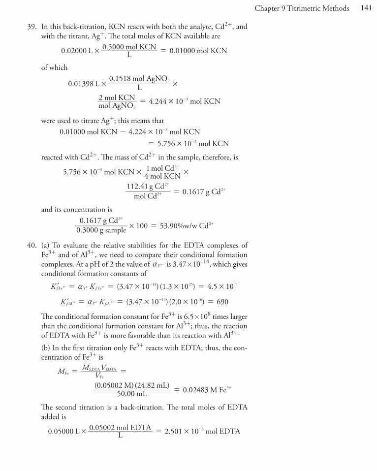
which means EDTA reacts with Ca2+ before it reacts with Mg2+. As we add EDTA, the exothermic reaction of EDTA and Ca2+ causes the temperature to increase. Once we reach this reaction’s equivalence point , the temperature begins to drop as the endothermic reaction of EDTA and Mg takes over. After the second equivalence point, the temperature will continue to decrease as the solution cools. Figure SM9.19 shows an idealized thermometric titration curve for this sys-tem; note that actual shape of the titration curve at each equivalence point and the rate of change in temperature after the second equiva-lence point will depend upon the reaction conditions, including the properties of the vessel in which the titration is carried out.
35. The best choice is the titrant with the largest difference in logKf val-ues; in this case, the best choice is EGTA.
36. At the equivalence point, the moles of Ca2+ in the sample equal the moles of EDTA; thus
2.68 10 L L0.0119 mol EDTA
mol EDTA1 mol Ca
mol Ca40.08 g Ca
g1000 mg
0.128 mg Ca
4# # # #
# =
-
This is the mass of calcium in 0.100 mL; scaling up by a factor of 1000 gives the concentration of calcium as 128 mg per 100 mL.
37. The mass of CaCO3 in the sample as analyzed is
0.04411 L L0.04988 mol EDTA
mol EDTA1 mol Ca
mol Ca.0 g CaCO
0.2202 g CaCO100 9 3
3
# #
# =
This is the mass of CaCO3 in a 10.00-mL portion of the solution that contains the dissolved eggshell; thus, the %w/w CaCO3 in the eggshell is
5.613 g sample0.2002 g CaCO 10.00 mL
250.0 mL100 98.08%w/w CaCO
3
3
## =
38. The mass of NaCN in the sample as analyzed is
.
0.02736 L L0.1012 mol AgNO
1 mol AgNO2 mol NaCN
mol NaCN49 01 g NaCN
g1000 mg
271.4 mg NaCN
3
3# #
# # =
This is the mass of NaCN in a 5.00-mL sample drawn from the electroplating bath; thus, the concentration of NaCN in the electro-plating bath is
5.00 10 L samplemg271.4 NaCN
5.43 10 ppm NaCN34
##=-
volume of titrant (mL)
tem
pera
ture
Veq.pt. for Ca2+
Veq.pt. for Mg2+
Figure SM9.19 Thermometric titration curve for Problem 9.34. The green branch of the titration curve is the titration of Ca2+ using EDTA and the blue branch of the titration curve is the titration of Mg2+ with EDTA. Once the titration of Mg2+ is complete, the temperature continues to de-crease, as shown by the curve’s red branch. The straight-line segments represent an idealized titration curve; as suggested by the dashed lines, the actual shape of the titration curve at each equivalence point depends on the reaction conditions.
Note that we do not need to worry about the fact that the original 5.00 mL sample is diluted to 250.0 mL prior to its analysis. The only source of the 271.4 mg of NaCN is the 5.00 mL sample drawn from the electroplating bath. Contrast this with the previous problem where the source of the 0.2002 g of CaCO3 is a 10.00-mL sample drawn from a much larger volume of sam-ple that contains the dissolved eggshell.
141Chapter 9 Titrimetric Methods
39. In this back-titration, KCN reacts with both the analyte, Cd2+, and with the titrant, Ag+. The total moles of KCN available are
0.02000 L L0.5000 KCN 0.01000 mol KCNmol# =
of which
0.01398 L L0.1518 mol
mol AgNO2 mol KCN 4.244 10 mol KCN
AgNO
3
3
3# #
#= -
were used to titrate Ag+; this means that0.01000 mol KCN 4.224 10 mol KCN
5.756 10 mol KCN
3
3
#
#
-
=
-
-
reacted with Cd2+. The mass of Cd2+ in the sample, therefore, is
5.756 10 mol KCN 4 mol KCN1 mol Cd
mol Cd112.41 g Cd
0.1617 g Cd
32
2
22
# # #
=
-+
+
+
+
and its concentration is
0.3000 g sample0.1617 g Cd
100 53.90%w/w Cd2
2# =+
+
40. (a) To evaluate the relative stabilities for the EDTA complexes of Fe3+ and of Al3+, we need to compare their conditional formation complexes. At a pH of 2 the value of Y4a - is 3.47×10⁻¹⁴, which gives conditional formation constants of
( . ) ( . ) .K K 3 47 10 1 3 10 4 5 10, ,f f14 25 11
Fe Y Fe3 4 3 # # #a= = =-+ - +l
( . ) ( ).K K 3 47 10 102 0 690, ,f f14 16
YAl Al3 4 3 # #a= = =-+ - +l
The conditional formation constant for Fe3+ is 6.5×10⁸ times larger than the conditional formation constant for Al3+; thus, the reaction of EDTA with Fe3+ is more favorable than its reaction with Al3+.
(b) In the first titration only Fe3+ reacts with EDTA; thus, the con-centration of Fe3+ is
M VM V
50.00 mL(0.05002 M)(24.82 mL) 0.02483 M Fe
FeFe
EDTA EDTA
3
= =
= +
The second titration is a back-titration. The total moles of EDTA added is
0.05000 L L0.05002 mol EDTA 2.501 10 mol EDTA3# #= -
142 Solutions Manual for Analytical Chemistry 2.1
of which
0.01784 L L0.04109 mol Fe
mol Fe1 mol EDTA 7.33 10 mol EDTA
3
34
# #
#=
+
+-
react with Fe3+, leaving us with
.1 7682.501 10 7.33 10 10 mol EDTA3 4 3# # #- =- - -
to react with Al3+. The concentration of Al3+, therefore, is
1.768 10 mol EDTA mol EDTA1 mol Al
0.05000 L 0.03536 M Al3
3
3# #
=
-+
+
41. (a) To show that a precipitate of PbSO4 is soluble in a solution of EDTA, we add together the first two reactions to obtain the reaction
( ) ( ) ( ) ( )s aq aq aqPbSO Y PbY SO44 2
42?+ +- - -
for which the equilibrium constant is
( . ) ( . ) .K K K 1 6 10 1 1 10 1 8 108 18 10sp f,PbY2 # # #= = =-
-
The large magnitude of the equilibrium constant means that PbSO4 is soluble in EDTA.
(b) The displacement of Pb2+ from PbY4– by Zn2+ is the reaction
( ) ( ) ( ) ( )aq aq aq aqPbY Zn ZnY Pb2 22 2?+ +- + - +
for which the equilibrium constant is
.
. .K KK
1 1 103 2 10 0 02918
16
f,PbY
f,ZnY
2
2
##= = =
-
-
Although less than 1, the equilibrium constant does suggest that there is some displacement of Pb2+ when using Zn2+ as the titrant. When using Mg2+ as the titrant, the potential displacement reaction
( ) ( ) ( ) ( )aq aq aq aqPbY MgY PbMg2 22 2?+ +- + - +
has an equilibrium constant of
.. .K K
K1 1 104 9 10 4 5 1018
810
f,PbY
f,MgY
2
2
## #= = = -
-
-
As this is a much smaller equilibrium constant, the displacement of Pb2+ by Mg2+ is not likely to present a problem. Given the equilib-rium constants, we will underestimate the amount of sulfate in the sample if we use Zn2+ as the titrant. To see this, we note that for this back-titration the total moles of EDTA used is equal to the combined moles of Pb2+ and of Zn2+. If some of the Zn2+ displaces Pb2+, then we use more Zn2+ than expected, which means we underreport the moles of Pb2+ and, therefore, the moles of sulfate.
143Chapter 9 Titrimetric Methods
(c) The total moles of EDTA used is
0.05000 L L0.05000 mol EDTA 0.002500 mol EDTA# =
of which
0.01242 L L0.1000 mol Mg
mol Mg1mol EDTA 0.001242 mol EDTA
2
2
# #
=
+
+
react with Mg2+; this leaves
0.002500 0.001242 0.001258 mol EDTA- =
to react with Pb2+. The concentration of sulfate in the sample, there-fore, is
0.001258 mol EDTA mol EDTA1 mol Pb
mol Pb1 mol SO 0.001258 mol SO
2
242
42
# #
=
+
+
--
0.02500 L0.001258 mol SO 0.05032 M SO4
2
42=
--
42. Let’s start by writing an equation for Y4a - that includes all seven forms of EDTA in solution
[H Y ] [H Y ] [H Y][H Y ] [H Y ] [HY ] [Y ]
[Y ]Y
62
5 4
3 22 3 4
4
4a =+ + +
+ + +
+ +
- - - -
-
-
) 3
Next, we define the concentration of each species in terms of the con-centration of Y4–; for example, using the acid dissociation constant, Ka6, for HY3–
K [HY ][Y ][H O ]
a6 3
43= -
- +
we have
K[HY ] [Y ][H O ]3
a6
43=-
- +
and using the acid dissociation constant, Ka5, for H2Y2–
K [H Y ][HY ][H O ]
225a
33= -
- +
we have
K K K[H Y ] [HY ][H O ] [Y ][H O ]2
2
5 5
2
a
33
a a6
43= =-
- + - +
Continuing in this fashion—the details are left to you—we find that
144 Solutions Manual for Analytical Chemistry 2.1
K K K[H Y ] [Y ][H O ]3
5
3
4a a a6
43=-
- +
K K K K[H Y] [Y ][H O ]4 5
43
4
a a a a6
43=
- +
K K K K K[H Y ] [Y ][H O ]3 4 5
52
5
a a a a a6
43=+
- +
K K K K K K[H Y ] [Y ][H O ]6
2
1 2 3 4 5
6
a a a a a a6
43=+
- +
Now things get a bit messy (!) as we substitute each of the last six equations back into our equation for Y4a -
K K K K K K K K K K K
K K K K K K K
K K K
[Y ][H O ] [Y ][H O ]
[Y ][H O ] [Y ][H O ]
[Y ][H O ] [Y ][H O ] [Y ]
[Y ]
1 2 3 4 5
6
2 3 4 5
5
3 4 5
4
4 5
3
5
2
Y
a a a a a a6
43
a a a a a6
43
a a a a6
43
a a a6
43
a a6
43
a6
43 4
4
4a =+ +
+ +
+ +
- + - +
- + - +
- + - +-
-
- Z
[
\
]]]
]]]
_
`
a
bbb
bbb
This equation looks imposing, but we can simplify it by factoring [Y4–] out of the denominator and simplifying
K K K K K K K K K K K
K K K K K K K
K K K 1
1[H O ] [H O ]
[H O ] [H O ]
[H O ] [H O ]
1 2 3 4 5
6
2 3 4 5
5
3 4 5
4
4 5
3
5
2
Y
a a a a a a6
3
a a a a a6
3
a a a a6
3
a a a6
3
a a6
3
a6
3
4a =+ +
+ +
+ +
+ +
+ +
+ +
- Z
[
\
]]]
]]]
_
`
a
bbb
bbb
and then multiplying through by Ka1Ka2Ka3Ka4Ka5Ka6 to arrive at our final equation
K K KK K K K K K K
K K K K K K K K K K K
K K K K K K[H O ] [H O ] [H O ]
[H O ] [H O ][H O ]
61
51 2
4
1 2 33
1 2 3 42
1 2 3 4 5 1 2 3 4 5
1 2 3 4 5Y
3 a 3 a a 3
a a a 3 a a a a 3
a a a a a 3 a a a a a a6
a a a a a a64a =
+ + +
+ +
+
+ + +
+ +
+
- Z
[
\
]]
]
_
`
a
bb
b
43. (a) The titration of V2+ with Ce4+ is an example of a redox titration. The titration’s equivalence point is reached when
n M V M V nV V Ce CeV Ce= = =
where n is the moles of V2+ or of Ce4+; thus
V V MM V
00 25 25(0. 100 M)
(0. 100 M)( .0 mL) .0 mL. .eq pt CeCe
V V= = = =
Before the equivalence point, the potential is easiest to calculate by using the Nernst equation for the analyte’s half-reaction
For the titration curves in this problem, we will calculate the potential for one volume of titrant before the equivalence point and the potential for one volume of titrant after the equivalence point.
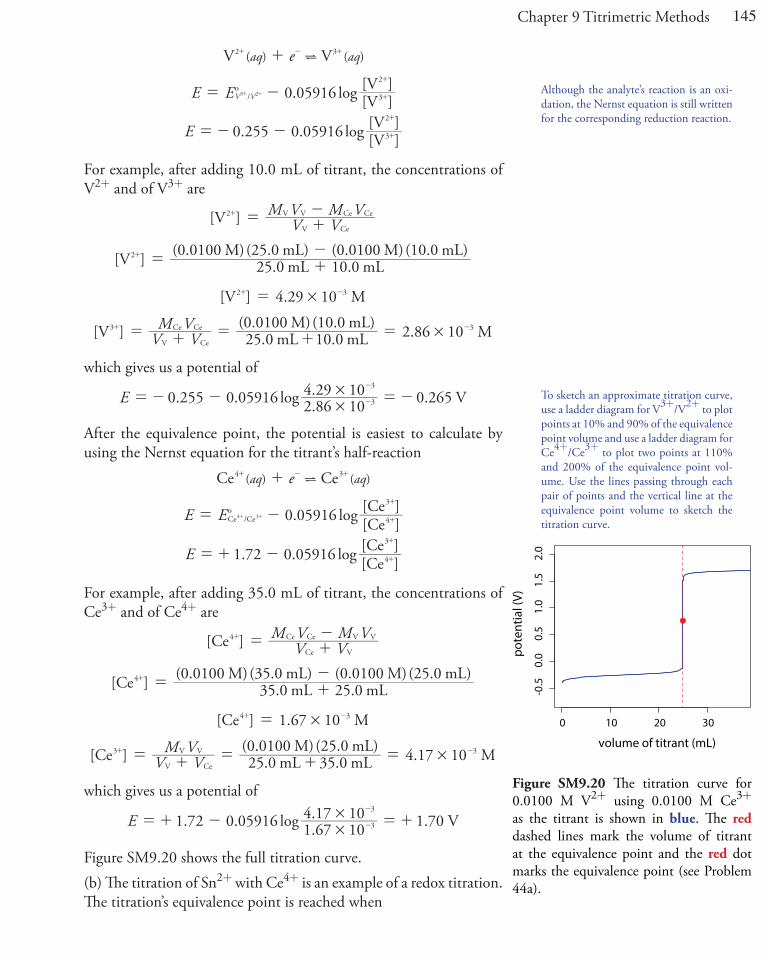
145Chapter 9 Titrimetric Methods
( ) ( )eaq aqV V2 3?++ - +
.
. .
log
log
E E
E
0 05916
0 255 0 05916
[V ][V ]
[V ][V ]
/V Vo
3
2
3
2
3 2= -
=- -
+
+
+
+
+ +
For example, after adding 10.0 mL of titrant, the concentrations of V2+ and of V3+ are
] V VM V M V[V2
V Ce
V V Ce Ce= +-+
[V ] 25.0 mL 10.0 mL(0.0100 M)(25.0 mL) (0.0100 M)(10.0 mL)2 = +
-+
.4 29 10[V ] M32 #=+ -
.V VM V 2 86 10[V ] 25.0 mL 10.0 mL
(0.0100 M)(10.0 mL) M33
V Ce
Ce Ce #= + = + =+ -
which gives us a potential of
. . .. .logE 0 255 0 05916 2 86 10
4 29 10 0 265 V3
3
##=- - =--
-
After the equivalence point, the potential is easiest to calculate by using the Nernst equation for the titrant’s half-reaction
( ) ( )eaq aqCeCe4 3?++ - +
.
. .
log
log
E E
E
0 05916
1 72 0 05916
[Ce ][Ce ]
[Ce ][Ce ]
Ce /Ceo
4
3
4
3
4 3= -
=+ -
+
+
+
+
+ +
For example, after adding 35.0 mL of titrant, the concentrations of Ce3+ and of Ce4+ are
] V VM V M V[Ce4
Ce V
Ce Ce V V= +-+
3 253 25[Ce ] 5.0 mL .0 mL
(0.0100 M)( 5.0 mL) (0.0100 M)( .0 mL)4 = +-+
. 101 67[Ce ] M4 3#=+ -
.V VM V
3525 4 17 10[Ce ] 25.0 mL .0 mL
(0.0100 M)( .0 mL) M33
V Ce
V V #= + = + =+ -
which gives us a potential of
. . .. .logE 1 72 0 05916 1 67 10
4 17 10 1 70 V3
3
##=+ - =+-
-
Figure SM9.20 shows the full titration curve. (b) The titration of Sn2+ with Ce4+ is an example of a redox titration.
The titration’s equivalence point is reached when
To sketch an approximate titration curve, use a ladder diagram for V3+/V2+ to plot points at 10% and 90% of the equivalence point volume and use a ladder diagram for Ce4+/Ce3+ to plot two points at 110% and 200% of the equivalence point vol-ume. Use the lines passing through each pair of points and the vertical line at the equivalence point volume to sketch the titration curve.
0 10 20 30
-0.5
0.0
0.5
1.0
1.5
2.0
volume of titrant (mL)
pote
ntia
l (V)
Figure SM9.20 The titration curve for 0.0100 M V2+ using 0.0100 M Ce3+ as the titrant is shown in blue. The red dashed lines mark the volume of titrant at the equivalence point and the red dot marks the equivalence point (see Problem 44a).
Although the analyte’s reaction is an oxi-dation, the Nernst equation is still written for the corresponding reduction reaction.
146 Solutions Manual for Analytical Chemistry 2.1
n M V M V n2Sn Sn Sn Ce CeCe#= = =
where n is the moles of Sn2+ or of Ce4+; thus
( )
V V MM V2
02 0 25 50(0. 100 M)
(0. 100 M)( .0 mL) .0 mL
. .eq pt CeCe
Sn Sn#= = =
=
Before the equivalence point, the potential is easiest to calculate by using the Nernst equation for the analyte’s half-reaction
( ) ( )eaq aq2Sn Sn42 ?++ - +
.
. .
log
log
E E
E
0 05916
0 154 0 059162
2
[ ][ ]
[Sn ][Sn ]SnSn
/Sno
4
2
4
2
Sn4 2= -
=+ -
+
+
+
+
+ +
For example, after adding 10.0 mL of titrant, the concentrations of Sn2+ and of Sn4+ are
] .V V
M V M V0 5[Sn2
Sn Ce
Sn Sn Ce Ce#= +-+
( . )0 5[Sn ] 25.0 mL 10.0 mL(0.0100 M)(25.0 mL) (0.0100 M)(10.0 mL)2 = +
-+
.5 71[Sn ] 10 M2 3#=+ -
.
( . ) .
V VM V0 5
0 5 101 43
[Sn ]
25.0 mL 10.0 mL(0.0100 M)(10.0 mL) M
4
3
Ce
Ce
Sn
Ce#
#
= + =
+ =
+
-
which gives us a potential of
. ... .logE 0 154 2
0 059161 43 105 71 10 0 136 V3
3
##= - =-
-
After the equivalence point, the potential is easiest to calculate by using the Nernst equation for the titrant’s half-reaction
( ) ( )eaq aqCeCe4 3?++ - +
.
. .
log
log
E E
E
0 05916
1 72 0 05916
[Ce ][Ce ]
[Ce ][Ce ]
Ce /Ceo
4
3
4
3
4 3= -
=+ -
+
+
+
+
+ +
For example, after adding 60.0 mL of titrant, the concentrations of Ce3+ and of Ce4+ are
] V VM V M V2[Ce4
Ce Sn
Ce Ce SnSn#= +-+
( )25
60 2 2560[Ce ] .0 mL .0 mL
(0.0100 M)( .0 mL) (0.0100 M)( .0 mL)4 =+-+
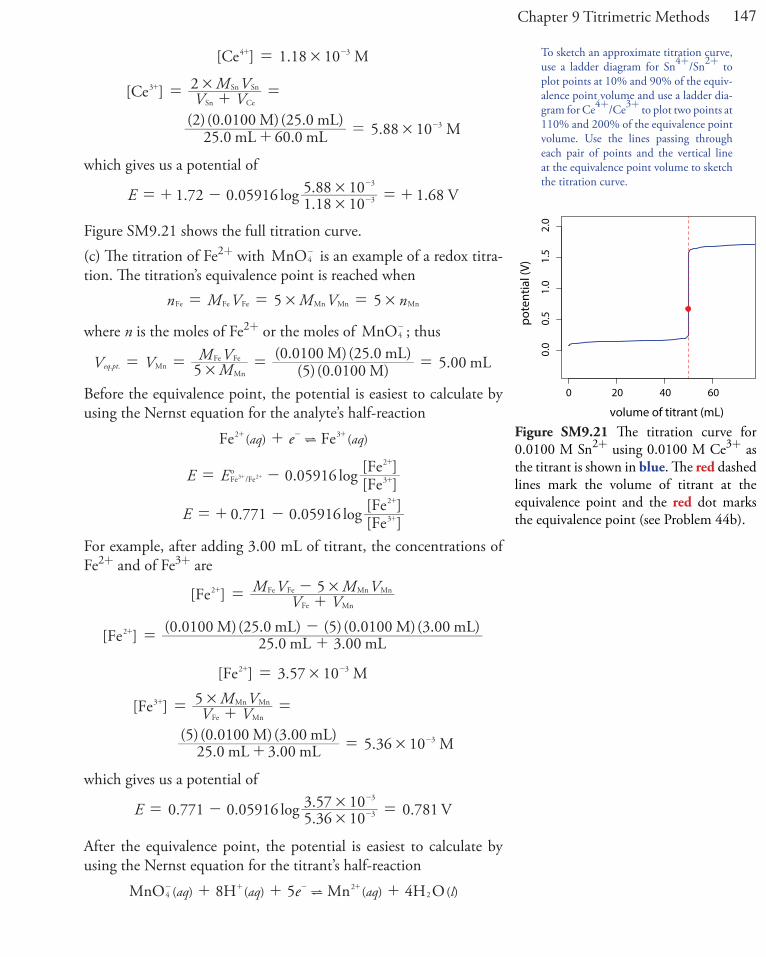
147Chapter 9 Titrimetric Methods
.1 18 10[Ce ] M4 3#=+ -
( ) .
V VM V2
602 25 5 88 10
[Ce ]
25.0 mL .0 mL(0.0100 M)( .0 mL) M3
3
Sn Ce
Sn Sn#
#
= + =
+=
+
-
which gives us a potential of
. . .. .logE 1 72 0 05916 1 18 10
5 88 10 1 68 V3
3
##=+ - =+-
-
Figure SM9.21 shows the full titration curve. (c) The titration of Fe2+ with MnO4
- is an example of a redox titra-tion. The titration’s equivalence point is reached when
n M V M V n5 5Fe Fe Fe Mn Mn Mn# #= = =
where n is the moles of Fe2+ or the moles of MnO4- ; thus
( )V V MM V
5 5 00 25 5 0(0. 100 M)
(0. 100 M)( .0 mL) .0 mL. .eq ptMn
FeMn
Fe
#= = = =
Before the equivalence point, the potential is easiest to calculate by using the Nernst equation for the analyte’s half-reaction
( ) ( )eaq aqFe Fe32 ?++ - +
.
. .
log
log
E E
E
0 05916
0 771 0 05916
[Fe ][Fe ]
[Fe ][Fe ]
3
3
Fe /Feo
2
2
3 2= -
=+ -
+
+
+
+
+ +
For example, after adding 3.00 mL of titrant, the concentrations of Fe2+ and of Fe3+ are
] V VM V M V5[Fe2
Fe Mn
Fe MnFe Mn#= +-+
( )3 0
5 3 0[Fe ] 25.0 mL . 0 mL(0.0100 M)(25.0 mL) (0.0100 M)( . 0 mL)2 = +
-+
[Fe ] 3.57 10 M2 3#=+ -
( ) .
V VM V5
3 05 3 0 105 36
[Fe ]
25.0 mL . 0 mL(0.0100 M)( . 0 mL) M
3
3
Mn
Mn
Fe
Mn#
#
= + =
+ =
+
-
which gives us a potential of
. . .. .logE 0 771 0 05916 5 36 10
3 57 10 0 781 V3
3
##= - =-
-
After the equivalence point, the potential is easiest to calculate by using the Nernst equation for the titrant’s half-reaction
( ) ( ) ( ) ( )eaq aq aq l5 4MnO 8H Mn H O42
2?+ + +- + - +
To sketch an approximate titration curve, use a ladder diagram for Sn4+/Sn2+ to plot points at 10% and 90% of the equiv-alence point volume and use a ladder dia-gram for Ce4+/Ce3+ to plot two points at 110% and 200% of the equivalence point volume. Use the lines passing through each pair of points and the vertical line at the equivalence point volume to sketch the titration curve.
0 20 40 60
0.0
0.5
1.0
1.5
2.0
volume of titrant (mL)
pote
ntia
l (V)
Figure SM9.21 The titration curve for 0.0100 M Sn2+ using 0.0100 M Ce3+ as the titrant is shown in blue. The red dashed lines mark the volume of titrant at the equivalence point and the red dot marks the equivalence point (see Problem 44b).
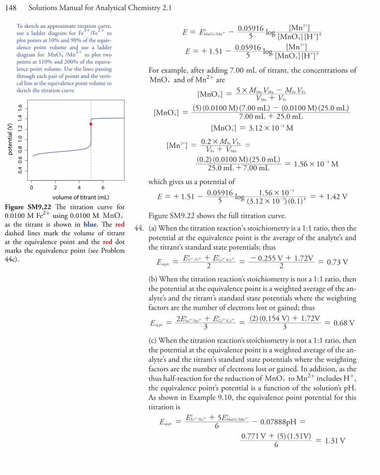
148 Solutions Manual for Analytical Chemistry 2.1
.
. .
log
log
E E
E
50 05916
1 51 50 05916
[MnO ][H ][Mn ]
[MnO ][H ][Mn ]
MnO /Mno
48
2
48
2
42= -
=+ -
- +
+
- +
+
- +
For example, after adding 7.00 mL of titrant, the concentrations of MnO4
- and of Mn2+ are
] V VM V M V5[MnO4
Mn Fe
Mn FeMn Fe#= +--
[ ] mL 25.0 mL(5)(0.0100 M)( .00 mL) (0.0100 M)(25.0 mL)MnO 7.00
74 = +
--
[MnO ] 3.12 10 M43#=- -
.
( . ) .
V VM V0 2
00 2 25 1 56 107
[Mn ]
25.0 mL . 0 mL(0.0100 M)( .0 mL) M
2
3
Fe
Fe
Mn
Fe#
#
= + =
+ =
+
-
which gives us a potential of
. .( . ) ( . )
. .logE 1 51 50 05916
3 12 10 0 11 56 10 1 42 V3
3
8##=+ - =+-
-
Figure SM9.22 shows the full titration curve.44. (a) When the titration reaction's stoichiometry is a 1:1 ratio, then the
potential at the equivalence point is the average of the analyte’s and the titrant’s standard state potentials; thus
E E E2 2
0.255 V 1.72V 0.73 V. .eq ptV /Vo
Ce /Ceo
3 2 4 3
=+
= - + =+ + + +
(b) When the titration reaction’s stoichiometry is not a 1:1 ratio, then the potential at the equivalence point is a weighted average of the an-alyte’s and the titrant’s standard state potentials where the weighting factors are the number of electrons lost or gained; thus
E E E3
23
(2)(0.154 V) 1.72V 0.68 V. .eq ptSn /Sno
Ce /Ceo
4 2 4 3
=+
=+
=+ + + +
(c) When the titration reaction’s stoichiometry is not a 1:1 ratio, then the potential at the equivalence point is a weighted average of the an-alyte’s and the titrant’s standard state potentials where the weighting factors are the number of electrons lost or gained. In addition, as the thus half-reaction for the reduction of MnO4
- to Mn2+ includes H+, the equivalence point’s potential is a function of the solution’s pH. As shown in Example 9.10, the equivalence point potential for this titration is
.E E E65 0 07888pH
60.771 V (5)(1.51V) 1.31 V
. .eq ptFe /Feo
MnO /Mno
3 24
2
=+
- =
+=
+ + - +
To sketch an approximate titration curve, use a ladder diagram for Fe3+/Fe2+ to plot points at 10% and 90% of the equiv-alence point volume and use a ladder diagram for MnO4
- /Mn2+ to plot two points at 110% and 200% of the equiva-lence point volume. Use the lines passing through each pair of points and the verti-cal line at the equivalence point volume to sketch the titration curve.
0 2 4 6
0.4
0.6
0.8
1.0
1.2
1.4
1.6
volume of titrant (mL)
pote
ntia
l (V)
Figure SM9.22 The titration curve for 0.0100 M Fe2+ using 0.0100 M MnO4
- as the titrant is shown in blue. The red dashed lines mark the volume of titrant at the equivalence point and the red dot marks the equivalence point (see Problem 44c).
149Chapter 9 Titrimetric Methods
45. (a) With an equivalence point potential of 0.73 V, diphenylamine, which has a standard state potential of 0.75 V, is an appropriate indi-cator.
(b) With an equivalence point potential of 0.68 V, diphenylamine, which has a standard state potential of 0.75 V, is an appropriate indi-cator.
(c) With an equivalence point potential of 1.31 V, tris(5-ni-tro-1,10-phenanthroline)iron, which has a standard state potential of 1.25 V, is an appropriate indicator.
46. (a) The procedure requires that we remove any excess Sn2+ so that it does not react with the titrant and cause a determinate error in the analysis for iron. To remove Sn2+, the procedure uses Hg2+ to oxi-dize it to Sn4+, with the Hg2+ forming a precipitate of Hg2Cl2. If we do not observe a precipitate, then excess Sn2+ is not present, which means we failed to reduce all the analyte from Fe3+ to Fe2+. If a gray precipitate forms, then too much Sn2+ is present, reducing Hg2+ to Hg instead of to Hg2Cl2. This is a problem because it means we did may not have oxidize all the Sn2+.
(b) No. The first addition of Sn2+ is used simply to speed up the dissolution of the ore.
(c) No. In the next step the Fe3+ is reduced back to Fe2+.47. We use volumetric glassware when we need to know the exact volume
as part of a calculation. Of the volumes highlighted in the procedure, we need to know only two with any certainty: the volume of sample taken (“A 50-mL portion of the resulting solution...”) and the volume of Fe2+ added in excess (“...50 mL of a standard solution of Fe2+...”).
48. (a) Because the titrant, KMnO4, reacts with the stabilizer, we use more titrant than expected and report a concentration of H2O2 that is greater than expected.
(b) The simplest approach is to prepare and analyze a reagent blank by replacing the 25 mL of sample with 25 mL of distilled water that has been treated to remove any traces of dissolved organic matter. We then subtract he volume of titrant used to analyze the reagent blank from the volume of titrant used to analyze the sample.
(c) Because the concentration of H2O2 is 5× greater, the volume of KMnO4 used in the titration will increase by a factor of five as well. To ensure that the titration’s end point does not exceed the buret’s maximum volume, we must either change the way the sample is pre-pared to reduce the concentration of H2O2 by a factor of five, or use a more concentrated solution of KMnO4 as the titrant. For example, to change the concentration of H2O2, we can take a 5-mL sample in place of a 25-mL sample.
150 Solutions Manual for Analytical Chemistry 2.1
49. In the titration reaction, each iron loses one electron as it is oxidized from Fe2+ to Fe3+, and each manganese gains five electrons as it is reduced from MnO4
- to Mn2+. The stoichiometry of the reaction, therefore, requires that five moles of Fe2+ react with each mole of MnO4
- ; thus, there are
0.04127 L L0.02500 mol MnO
mol MnO5 mol Fe Fe5.159 10 mol
4
4
223
# #
#=
-
-
++-
in the sample as analyzed. The concentration of Fe2O3 in the original sample is
5.159 10 mol Fe 2 mol Fe1 mol Fe O
mol Fe O159.69 g Fe O
0.4119 g Fe O
3 22
2 3
2 3
2 32 3
# #
# =
- ++
0.4185 g sample0.4119 g Fe O
100 98.42%w/w Fe O2 32 3# =
50. In the titration reaction, each manganese in the analyte loses two electrons as it is oxidized from Mn2+ to MnO2, and each manganese in the titrant gains three electrons as it is reduced from MnO4
- to MnO2. The stoichiometry of the reaction, therefore, requires that three moles of Mn2+ react with two moles of MnO4
- ; thus, there are
0.03488 L L0.03358 mol MnO
2 mol MnO3 mol Mn
mol Mn54.938 g Mn
0.09652 g Mn
4
4
2
2
22
# #
# =
-
-
+
+
+
+
in the sample as analyzed. The concentration of Mn2+ in the original sample is
0.5165 g sample0.09652 g Mn
100 18.69%w/w Mn2
2# =+
+
51. In this indirect titration, iron, in the form of Fe3+, reacts with the analyte, uranium, and then, in the form of Fe2+, with the titrant, K2Cr2O7. In its reaction with the analyte, iron gains one electron as it is reduced from Fe3+ to Fe2+, and uranium loses two electrons as it is oxidized from U4+ to U6+; thus, each mole of U4+ produces two moles of Fe2+. In its reaction with the titrant, iron loses one electron as it is oxidized from Fe2+ to Fe3+ and each chromium gains three electrons as it is reduced from Cr O2 7
2- to Cr3+; thus, the stoichiome-try of the titration reaction requires that six moles of Fe2+ reacts with each mole of Cr O2 7
2- . The titration with K2Cr2O7 shows us that the moles of Fe2+ formed using the Walden reductor is
For a redox titration, we can determine the reaction’s stoichiometry by consider-ing the changes in oxidation states expe-rienced by the analyte and by the titrant without working out the balanced reac-tion. Of course, we can write the balanced reaction as well, which, in this case, is
( ) ( ) ( )
( ) ( ) ( )
aq aq aq
aq aq l
5
5 4
Fe MnO 8H
Fe Mn H O
24
3 22
?+ +
+ +
+ - +
+ +
151Chapter 9 Titrimetric Methods
.6 6 23
0.01052 L L0.00987 mol K Cr O
mol K Cr Omol Fe 10 mol Fe4
2 2 7
2 2 7
22
# #
#=+
- +
which means the original sample contained
. .6 23 3 1210 mol Fe 2 mol Fe1 mol U 10 mol U4 42
2
44# # #=- +
+
+- +
The concentration of uranium in the original sample, therefore is
..
3 1223 60.315 g sample
10 mol U mol U238.08 g U
100 %w/w U4 4
4
4
4# #
# =
- ++
+
+
52. In this back-titration, iron, in the form of Fe2+, reacts with the ana-lyte, chromium, and then with the titrant, K2Cr2O7. In its reaction with the analyte, iron loses one electron as it is oxidized from Fe2+ to Fe3+ and each chromium gains three electrons as it is reduced from Cr O2 7
2- to Cr3+; thus, six moles of Fe2+ reacts with each mole of Cr O2 7
2- . In its reaction with the titrant, iron loses one electron as it is oxidized from Fe2+ to Fe3+ and each chromium gains three electrons as it is reduced from Cr O2 7
2- to Cr3+; thus, the stoichiometry of the titration reaction requires that each mole of Fe2+ reacts with six moles of Cr O2 7
2- . The total moles of Fe2+ added to the original sample is
92 28
0.500 g Fe(NH ) (SO ) 6H O
3 .12 g Fe(NH ) (SO ) 6H O1 mol Fe 1. 10 mol Fe
4 2 4 2 2
4 2 4 2 2
23 2
: #
:#=
+- +
Of this iron, the moles that react with the titrant, K2Cr2O7 are
.6
829 389
4 27
0.01 L L0.00 mol K Cr O
mol K Cr Omol Fe 10 mol Fe4
2 2 7
2 2 7
22
# #
#=+
- +
which leaves 1.28×10⁻³ – 4.27×10–4 = 8.53×10⁻⁴ moles of Fe2+ to react with chromium in the original sample; thus, the mass of chromium in the original sample is
.8 53
49
10 mol Fe 6 mol Fe1 mol Cr O
mol Cr O2 mol Cr
mol Cr51.996 g Cr
0.01 g Cr
4 22
2 72
2 72
# #
# # =
- ++
-
-
and the thickness of chromium is
thickness areavolume
30.0 cm
0.0149 g 7.20 g1
mL1 cm
6.90 10 cm
mL
2
3
5# #
#
= =
= -
152 Solutions Manual for Analytical Chemistry 2.1
53. In this indirect titration, the analyte, CO, reacts with I2O5 to form CO2 and I2. In this reaction, carbon loses two electrons as its oxida-tion state changes from +2 to +4, and each iodine gains five electrons as its oxidation state changes from +5 to 0; thus, ten moles of CO produced two moles of I2. The I2 formed is converted to I3
- , which then is titrated with S O2 3
2- , forming I– and S O4 62- . In the titration
reaction, each iodine gains the equivalent of 2/3rd of an electron as its oxidation state changes from –1/3 to –1, and each sulfur loses the equivalent of 1/2 of an electron as its changes its oxidation state from +2 to +2.5; thus, each mole of I3
- reacts with two moles of S O2 32- .
Beginning with the moles of S O2 32- used in the titration
0.00717 L S O L0.00329 mol S O 2.36 10 mol S O2 3
2 32
52 3
2# #=--
- -
we use stoichiometry to find the mass of CO in the original sample
2.36 10 mol S O 2 mol S O1 mol I
mol I1 mol I
mol I1 mol I O 1.18 10 mol I O
52 3
2
2 32
3
3
2
2
2 5 52 5
# # #
# #=
- --
-
--
.10 5 901.18 10 mol I O 2 mol I Omol CO 10 mol CO5
2 52 5
5# # #=- -
. .5 90 1 6510 mol CO mol CO28.01 g CO
10 g CO35# # #=- -
The mass of air taken is
4.79 L L1000 mL
mL1.23 10 g
5.89 g3
# ##
=-
which makes the concentration of CO in the air
5.89 g air
1.65 10 g CO g10 µg
2.80 10 ppm CO3
6
2# #
#=
-
54. In the Winkler method, Mn2+ reacts with O2 to form MnO2 with manganese changing its oxidation state from +2 to +4, and each ox-ygen changing its oxidation state from 0 to –2; thus, each mole of O2 reacts with two moles of Mn2+. Subsequently, MnO2 reacts with I–, forming Mn2+ and I3
- with manganese changing its oxidation state from +4 to +2, and each iodine changing its oxidation state from –1 to the equivalent of –1/3; thus three moles of I– react with each mole of MnO2. Finally, as we saw in Problem 53, in the titration of I3- with S O2 3
2- , each mole of I3- reacts with two moles of S O2 3
2- . Beginning with the moles of S O2 3
2- used in the titration
.890 870 7 740.00 L S O L0.00 mol S O 10 mol S O2 3
2 32
52 3
2# #=--
- -
we use stoichiometry to find the mass of O2 in the original sample
153Chapter 9 Titrimetric Methods
10 mol S O 2 mol S O1 mol I
mol Imol I
3 mol I1 mol
2 mol MnO1 mol O 1. 10 mol O
7.74 3
MnO 94
52 3
2
2 32
3
3
2
2 52
2
# # #
# # #=
- --
-
-
-
--
1.94 10 mol O mol O31.998 g O
6.21 10 g O52
2
2 42# # #=- -
The concentration of O2 in the original sample, therefore, is
100.0 mL
6.21 10 g O g10 µg
6.21 ppm O4
2
6
2
# #=
-
55. The titration of KI with AgNO3 is an example of a precipitation titration. The titration’s equivalence point is reached when
n M V M V nI I Ag AgI Ag= = =
where n is the moles of I– or of Ag+; thus
V V MM V
05025 50 25(0. 00 M)
(0. 0 M)( .0 mL) .0 mL. .eq ptAg
IAg
I= = = =
Before the equivalence point, the concentration of I– is determined by the amount of excess I–, and the concentration of Ag+ is determined by the solubility of AgI in the presence of excess I–. For example, after adding 10.0 mL of AgNO3, we find that
] V VM V M V[I
I Ag
I I Ag Ag= +
--
[I ] 50.0 mL 10.0 mL(0.0250 M)(50.0 mL) (0.0500 M)(10.0 ml)
= +--
[I ] 0.0125 M=-
] .. .K0 0125
8 32 10 6 66 10[Ag ] [I M17
15sp,AgI # #= = =+-
--
which gives pI as 1.90 and pAg as 14.18. After the equivalence point, the concentration of Ag+ is determined by the amount of excess Ag+, and the concentration of I– is determined by the solubility of AgI in the presence of excess Ag+. For example, after adding 35.0 mL of AgNO3, we find that
] V VM V M V[Ag
Ag I
Ag Ag I I= +
-+
[ ] 35.0 mL 50.0 mL(0.0500 M)(35.0 mL) (0.0250 M)(50.0 ml)Ag = +
-+
[ ] MAg 5.88 10 3#=+ -
] . ..K 8 32 10 1 41 105 88 10[I [Ag ] M
1714
3sp,AgI # #
#= = =-
+
--
-
For the titration curves in this problem and in the next problem, we will calcu-late pAnalyte or pTitrant for one volume before each equivalence point and for one volume after the final equivalence point.
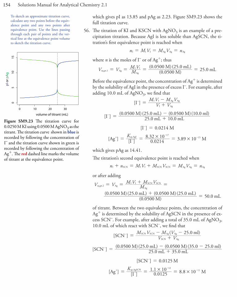
154 Solutions Manual for Analytical Chemistry 2.1
which gives pI as 13.85 and pAg as 2.23. Figure SM9.23 shows the full titration curve.
56. The titration of KI and KSCN with AgNO3 is an example of a pre-cipitation titration. Because AgI is less soluble than AgSCN, the ti-tration’s first equivalence point is reached when
n M V M V nI I Ag AgI Ag= = =
where n is the moles of I– or of Ag+; thus
V V MM V
05050 25 25(0. 00 M)
(0. 0 M)( .0 mL) .0 mLeq.pt.1 AgAg
I I= = = =
Before the equivalence point, the concentration of Ag+ is determined by the solubility of AgI in the presence of excess I–. For example, after adding 10.0 mL of AgNO3, we find that
] V VM V M V[I
I Ag
I I Ag Ag= +
--
2525
50[I ] .0 mL 10.0 mL(0.0 0 M)( .0 mL) (0.0500 M)(10.0 ml)
= +--
.0 0214[I ] M=-
] .. .K0 0
8 32 10 10214 3 89[Ag ] [I M17
15sp,AgI # #= = =+-
--
which gives pAg as 14.41. The titration’s second equivalence point is reached when
n n M V M V M V nI SCN I I SCN SCN Ag Ag Ag+ = + = =
or after adding
V V MM V M V
05050 25 050 25 50(0. 00 M)
(0. 0 M)( .0 mL) (0. 0 M)( .0 mL) .0 mL
eq.pt.2 AgAg
I I SCN SCN= = + =
+=
of titrant. Between the two equivalence points, the concentration of Ag+ is determined by the solubility of AgSCN in the presence of ex-cess SCN–. For example, after adding a total of 35.0 mL of AgNO3, 10.0 mL of which react with SCN–, we find that
] ( .V V
M V M V 25 0[ ml)SCNSCN Ag
SCN SCN Ag Ag= +
- --
. .25
50 25 35 0 25 035[SCN ] .0 mL .0 mL
(0.0 0 M)( .0 mL) (0.0500 M)( ml)= +
- --
[SCN ] 0.0 M125=-
] .. .K0 0125
10 101 1 8 8[Ag ] [I M1
112
sp,AgSCN # #= = =+-
--
To sketch an approximate titration curve, calculate any two points before the equiv-alence point and any two points after equivalence point. Use the lines passing through each pair of points and the ver-tical line at the equivalence point volume to sketch the titration curve.
0 10 20 30
05
1015
volume of titrant (mL)
pI o
r pA
g
Figure SM9.23 The titration curve for 0.0250 M KI using 0.0500 M AgNO3 as the titrant. The titration curve shown in blue is recorded by following the concentration of I– and the titration curve shown in green is recorded by following the concentration of Ag+. The red dashed line marks the volume of titrant at the equivalence point.
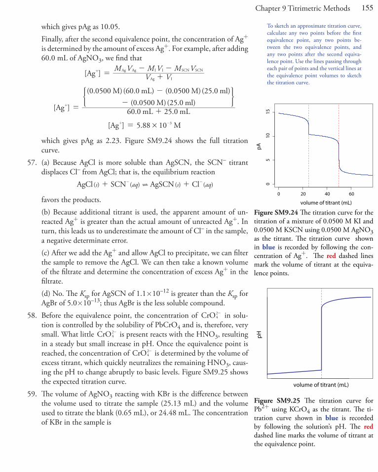
155Chapter 9 Titrimetric Methods
which gives pAg as 10.05. Finally, after the second equivalence point, the concentration of Ag+
is determined by the amount of excess Ag+. For example, after adding 60.0 mL of AgNO3, we find that
] V VM V M V M V[Ag
Ag I
Ag Ag I I SCN SCN= +
- -+
2560[Ag ] .0 mL .0 mL
(0.0500 M)(60.0 mL) (0.0500 M)(25.0 ml)(0.0500 M)(25.0 ml)
=+
-
-+
) 3
[ ] MAg 5.88 10 3#=+ -
which gives pAg as 2.23. Figure SM9.24 shows the full titration curve.
57. (a) Because AgCl is more soluble than AgSCN, the SCN– titrant displaces Cl– from AgCl; that is, the equilibrium reaction
( ) ( ) ( ) ( )s aq s aqAgCl SCN AgSCN Cl?+ +- -
favors the products. (b) Because additional titrant is used, the apparent amount of un-
reacted Ag+ is greater than the actual amount of unreacted Ag+. In turn, this leads us to underestimate the amount of Cl– in the sample, a negative determinate error.
(c) After we add the Ag+ and allow AgCl to precipitate, we can filter the sample to remove the AgCl. We can then take a known volume of the filtrate and determine the concentration of excess Ag+ in the filtrate.
(d) No. The Ksp for AgSCN of 1.1×10⁻¹² is greater than the Ksp for AgBr of 5.0×10⁻¹³; thus AgBr is the less soluble compound.
58. Before the equivalence point, the concentration of CrO42- in solu-
tion is controlled by the solubility of PbCrO4 and is, therefore, very small. What little CrO4
2- is present reacts with the HNO3, resulting in a steady but small increase in pH. Once the equivalence point is reached, the concentration of CrO4
2- is determined by the volume of excess titrant, which quickly neutralizes the remaining HNO3, caus-ing the pH to change abruptly to basic levels. Figure SM9.25 shows the expected titration curve.
59. The volume of AgNO3 reacting with KBr is the difference between the volume used to titrate the sample (25.13 mL) and the volume used to titrate the blank (0.65 mL), or 24.48 mL. The concentration of KBr in the sample is
To sketch an approximate titration curve, calculate any two points before the first equivalence point, any two points be-tween the two equivalence points, and any two points after the second equiva-lence point. Use the lines passing through each pair of points and the vertical lines at the equivalence point volumes to sketch the titration curve.
Figure SM9.24 The titration curve for the titration of a mixture of 0.0500 M KI and 0.0500 M KSCN using 0.0500 M AgNO3 as the titrant. The titration curve shown in blue is recorded by following the con-centration of Ag+. The red dashed lines mark the volume of titrant at the equiva-lence points.
Figure SM9.25 The titration curve for Pb2+ using KCrO4 as the titrant. The ti-tration curve shown in blue is recorded by following the solution’s pH. The red dashed line marks the volume of titrant at the equivalence point.
0 20 40 60
05
1015
volume of titrant (mL)
pA
volume of titrant (mL)
pH
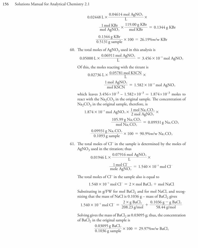
156 Solutions Manual for Analytical Chemistry 2.1
4
344
0.02 48 L L0.04614 mol AgNO
mol AgNO1 mol KBr
mol KBr119.00 g KBr
0.1 g KBr
3
3
# #
# =
0.5131 g sample0.1344 g KBr
100 26.19%w/w KBr# =
60. The total moles of AgNO3 used in this analysis is
0.05000 L L0.06911 mol AgNO
3.456 10 mol AgNO3 33# #= -
Of this, the moles reacting with the titrant is
0.02736 L L0.05781 mol KSCN
mol KSCN1 mol AgNO
1.582 10 mol AgNO3 33
# #
#= -
which leaves 3.456×10⁻³ – 1.582×10–3 = 1.874×10⁻³ moles to react with the Na2CO3 in the original sample. The concentration of Na2CO3 in the original sample, therefore, is
0
1.874 10 mol AgNO 2 mol AgNO1 mol Na CO
mol Na CO105.99 g Na CO
0. 9931 g Na CO
33
3
2 3
2 3
2 32 3
# # #
=
-
90.1093 g sample0.09931 g Na CO
100 90. %w/w Na CO2 32 3# =
61. The total moles of Cl– in the sample is determined by the moles of AgNO3 used in the titration; thus
0.01946 L L0.07916 mol AgNO
mole AgNO1 mol Cl 1.540 10 mol Cl
3
3
3
# #
#=-
- -
The total moles of Cl– in the sample also is equal to
1.540 10 mol Cl 2 mol BaCl mol NaCl32# #= +- -
Substituting in g/FW for mol BaCl2 and for mol NaCl, and recog-nizing that the mass of NaCl is 0.1036 g – mass of BaCl2 gives
1.540 10 mol Cl 208.23 g/mol2 g BaCl
58.44 g/mol0.1036 g g BaCl3 2 2
##
= +-- -
Solving gives the mass of BaCl2 as 0.03095 g; thus, the concentration of BaCl2 in the original sample is
0.03095 g BaCl0.1036 g sample 100 29.97%w/w BaCl2
2# =
Related Documents