Chapter 5dpuadweb.depauw.edu/harvey_web/eTextProject/SMFiles/Chpt... · 2016-06-02 · Chapter 5 Standardizing Analytical Methods 41 and solving for k A gives its value as 0.01583

39Chapter 5 Standardizing Analytical Methods

Chapter 5Many of the problems in this chapter require a regression analysis. Al-though equations for these calculations are highlighted in the solution to the first such problem, for the remaining problems, both here and elsewhere in this text, the results of a regression analysis simply are provided. Be sure you have access to a scientific calculator, a spreadsheet program, such as Excel, or a statistical software program, such as R, and that you know how to use it to complete a regression analysis.1. For each step in a dilution, the concentration of the new solution,

Cnew, is

C VC V

new

orig orignew =

where Corig is the concentration of the original solution, Vorig is the volume of the original solution taken, and Vnew is the volume to which the original solution is diluted. A propagation of uncertainty for Cnew shows that its relative uncertainty is

Cu

C V Vuu u

new

C

orig

C

orig

V

new

V2 2 2

new orig orig new= + +a a `k k j

For example, if we dilute 10.00 mL of the 0.1000 M stock solution to 100.0 mL, Cnew is 1.000×10–2 M and the relative uncertainty in Cnew is

.

...

.. .C

u0 10000 0002

10 000 02

100 00 08 2 94 10

new

C 2 2 23new #= + + = -` ` `j j j

The absolute uncertainty in Cnew, therefore, is

( . ) ( . ) .u 1 000 10 2 94 10 2 94 10M MC2 3 5

new # # # #= =- - -

The relative and the absolute uncertainties for each solution’s con-centration are gathered together in the tables that follow (all con-centrations are given in mol/L and all volumes are given in mL). The uncertainties in the volumetric glassware are from Table 4.2 and Table 4.3. For a Vorig of 0.100 mL and of 0.0100 mL, the uncertainties are those for a 10–100 µL digital pipet.

For a serial dilution, each step uses a 10.00 mL volumetric pipet and a 100.0 mL volumetric flask; thus

Cnew Corig Vorig Vnew uVorig uVnew

1.000×10–2 0.1000 10.00 100.0 0.02 0.08

1.000×10–3 1.000×10–2 10.00 100.0 0.02 0.08

1.000×10–4 1.000×10–3 10.00 100.0 0.02 0.08

1.000×10–5 1.000×10–4 10.00 100.0 0.02 0.08

See Chapter 4C to review the propagation of uncertainty.

40 Solutions Manual for Analytical Chemistry 2.1

Cnew Corig Cu

new

Cnew uCnew

1.000×10–2 0.1000 2.94×10–3 2.94×10–5

1.000×10–3 1.000×10–2 3.64×10–3 3.64×10–6

1.000×10–4 1.000×10–3 4.23×10–3 4.23×10–7

1.000×10–5 1.000×10–4 4.75×10–3 4.75×10–8

For the set of one-step dilutions using the original stock solution, each solution requires a different volumetric pipet; thus

Cnew Corig Vorig Vnew uVorig uVnew

1.000×10–2 0.1000 10.00 100.0 0.02 0.08

1.000×10–3 0.1000 1.000 100.0 0.006 0.08

1.000×10–4 0.1000 0.100 100.0 8.00×10–4 0.08

1.000×10–5 0.1000 0.0100 100.0 3.00×10–4 0.08

Cnew Corig Cu

new

Cnew uCnew

1.000×10–2 0.1000 2.94×10–3 2.94×10–5

1.000×10–3 0.1000 6.37×10–3 6.37×10–6

1.000×10–4 0.1000 8.28×10–3 8.28×10–7

1.000×10–5 0.1000 3.01×10–2 3.01×10–7

Note that for each Cnew, the absolute uncertainty when using a serial dilution always is equal to or better than the absolute uncertainty when using a single dilution of the original stock solution. More specifically, for a Cnew of 1.000×10–3 M and of 1.000×10–4 M, the improvement in the absolute uncertainty is approximately a factor of 2, and for a Cnew of 1.000×10–5 M, the improvement in the ab-solute uncertainty is approximately a factor of 6. This is a distinct advantage of a serial dilution. On the other hand, for a serial dilution a determinate error in the preparation of the 1.000×10–2 M solution carries over as a determinate error in each successive solution, which is a distinct disadvantage.

2. We begin by determining the value for kA in the equation

S k C Stotal A A reag= +

where Stotal is the average of the three signals for the standard of con-centration CA, and Sreag is the signal for the reagent blank. Making appropriate substitutions

. ( . ) .k0 1603 10 0 0 002ppmA= +

41Chapter 5 Standardizing Analytical Methods

and solving for kA gives its value as 0.01583 ppm–1. Substituting in the signal for the sample

. ( . ) .C0 118 0 01583 0 002ppm A1= +-

and solving for CA gives the analyte’s concentration as 7.33 ppm.3. This standard addition follows the format of equation 5.9

C VV

S

C VV C V

VS

Af

o

samp

Af

ostd

f

std

spike=

+

in which both the sample and the standard addition are diluted to the same final volume. Making appropriate substitutions

.

...

.

..

( . ).

C C 25 0010 00

25 0010 00

25 0010 00

0 2351 00

0 502

mLmL

mLmL

mLmLppmA A# # #

=+

. . .C C0 0940 0 0940 0 2008ppmA A+ =

and solving gives the analyte’s concentration, CA, as 0.800 ppm. The concentration of analyte in the original solid sample is

.

( . ) ( . ). %10 00

0 880 0 250 10001

100 2 20 10g sample

mg/L L mgg

w/w3# #= -

c m

4. This standard addition follows the format of equation 5.11

CS

C V VV C V V

VS

A

samp

Ao std

ostd

o std

std

spike=

+ + +

in which the standard addition is made directly to the solution that contains the analyte. Making appropriate substitutions

.

. ..

. .( . ) ( . )

.C

C

11 5

50 00 1 0050 00

50 00 1 0010 0 1 00

23 1

mL mLmL

mL mLppm mLA

A

=

+ + +

. . .C C23 1 11 27 2 255 ppmA A= +

and solving gives the analyte’s concentration, CA, as 0.191 ppm.5. To derive a standard additions calibration curve using equation 5.10

S k C V VV C V V

Vspike A A

o std

ostd

o std

std= + + +a k we multiply through both sides of the equation by Vo + Vstd

( )S V V k C V k C Vspike o std A A o A std std+ = +

As shown in Figure SM5.1, the slope is equal to kA and the y-inter-cept is equal to kACAVo. The x-intercept occurs when Sspike(Vo + Vstd) equals zero; thus

k C V k C V0 A A o A std std= +

slope = k A

y-intercept = kACAVo

x-intercept = –CAVo

S spik

e(Vo +

Vst

d)

CstdVstd

Figure SM5.1 Standard additions calibra-tion curve based on equation 5.10.

Here we assume that a part per million is equivalent to mg/L.

42 Solutions Manual for Analytical Chemistry 2.1

and the x-intercept is equal to –CAVo. We must plot the calibra-tion curve this way because if we plot Sspike on the y-axis versus

/ ( )C V V Vstd std o std# +" , on the x-axis, then the term we identify as y-intercept

V Vk C V

o std

A A o

+

is not a constant because it includes a variable,Vstd, whose value changes with each standard addition.

6. Because the concentration of the internal standard is maintained at a constant level for both the sample and the standard, we can fold the internal standard’s concentration into the proportionality constant K in equation 5.12; thus, using SA, SIS, and CA for the standard

.

. ( . )SS

k Ck C KC K0 233

0 155 10 00 mg/LIS

A

IS IS

A AA= = = =

gives K as 0.06652 L/mg. Substituting in SA, SIS, and K for the sample

.

. ( . )C0 2330 155 0 06652 L/mg A=

gives the concentration of analyte in the sample as 20.8 mg/L.7. For each pair of calibration curves, we seek to find the calibration

curve that yields the smallest uncertainty as expressed in the standard deviation about the regression, sr, the standard deviation in the slope, sb1 , or the standard deviation in the y-intercept, sb0 .

(a) The calibration curve on the right is the better choice because it uses more standards. All else being equal, the larger the value of n, the smaller the value for sr in equation 5.19, and for sb0 in equation 5.21.

(b) The calibration curve on the left is the better choice because the standards are more evenly spaced, which minimizes the term xi

2/ in equation 5.21 for sb0 .

(c) The calibration curve on the left is the better choice because the standards span a wider range of concentrations, which minimizes the term ( )x Xi

2-/ in equation 5.20 and in equation 5.21 for sb1 and sb0 , respectively.

8. To determine the slope and the y-intercept for the calibration curve at a pH of 4.6 we first need to calculate the summation terms that appear in equation 5.17 and in equation 5.18; these are:

..

..

xx y

yx

308 48397 5

131 019339 6

i

i i

i

i2

=

=

=

=

//

//

Substituting these values into the equation 5.17

( . ) ( . )( . ) ( . . ) .b 6 19339 6 308 46 8397 5 308 4 131 0 0 4771 2## #

=-

-=

As a reminder, for this problem we will work through the details of an unweight-ed linear regression calculation using the equations from the text. For the remain-ing problems, it is assumed you have access to a calculator, a spreadsheet, or a statistical program that can handle most or all of the relevant calculations for an unweighted linear regression.

43Chapter 5 Standardizing Analytical Methods

gives the slope as 0.477 nA/nM, and substituting into equation 5.18. ( . . ) .b 6

131 0 0 477 308 4 2 690#

=-

=-

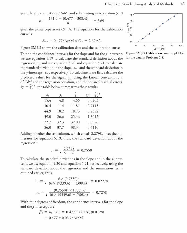
gives the y-intercept as –2.69 nA. The equation for the calibration curve is

. .S C0 477 2 69nA/nM nAtotal Cd#= -

Figure SM5.2 shows the calibration data and the calibration curve. To find the confidence intervals for the slope and for the y-intercept,

we use equation 5.19 to calculate the standard deviation about the regression, sr, and use equation 5.20 and equation 5.21 to calculate the standard deviation in the slope, sb1 , and the standard deviation in the y-intercept, sb0 , respectively. To calculate sr we first calculate the predicted values for the signal, yi

V , using the known concentrations of Cd2+ and the regression equation, and the squared residual errors, ( )y yi i

2-V ; the table below summarizes these results

xi yi yiV ( )y yi i

2-V15.4 4.8 4.66 0.020330.4 11.4 11.81 0.711544.9 18.2 18.73 0.238259.0 26.6 25.46 1.301272.7 32.3 32.00 0.092686.0 37.7 38.34 0.4110

Adding together the last column, which equals 2.2798, gives the nu-merator for equation 5.19; thus, the standard deviation about the regression is

. .s 6 22 2798 0 7550r = -

=

To calculate the standard deviations in the slope and in the y-inter-cept, we use equation 5.20 and equation 5.21, respectively, using the standard deviation about the regression and the summation terms outlined earlier; thus

( . ) ( . )( . ) .s 6 19339 6 308 4

6 0 7550 0 02278b 2

2

1 ##

=-

=

( . ) ( . )( . ) . .s 6 19339 6 308 40 7550 19339 6 0 7258b 2

2

0 ##

=-

=

With four degrees of freedom, the confidence intervals for the slope and the y-intercept are

. ( . ) ( . ). .

b ts 0 477 2 776 0 01280 477 0 036 nA/nM

b1 1 1! !

!

b = =

=

S tota

l (nA

)

[Cd2+] (nM)0 20 40 60 80 100

010

2030

40

Figure SM5.2 Calibration curve at pH 4.6 for the data in Problem 5.8.

44 Solutions Manual for Analytical Chemistry 2.1

. ( . ) ( . ). .

b ts 2 69 2 776 0 72582 69 2 01 nA

b1 0 0! !

!

b = =-

=-

(b) The table below shows the residual errors for each concentra-tion of Cd2+. A plot of the residual errors (Figure SM5.3) shows no discernible trend that might cause us to question the validity of the calibration equation.

xi yi yiV y yi i-V

15.4 4.8 4.66 0.1430.4 11.4 11.81 –0.4144.9 18.2 18.73 –0.5359.0 26.6 25.46 1.1472.7 32.3 32.00 0.3086.0 37.7 38.34 –0.64

(c) A regression analysis for the data at a pH of 3.7 gives the calibra-tion curve’s equation as

. .S C1 43 5 02nA/nM nAtotal Cd#= -

The more sensitive the method, the steeper the slope of the cali-bration curve, which, as shown in Figure SM5.4, is the case for the calibration curve at pH 3.7. The relative sensitivities for the two pHs is the ratio of their respective slopes

.. .k

k0 4771 43 3 00

.

.

4 6

3 7

pH

pH= =

The sensitivity at a pH of 3.7, therefore, is three times more sensitive than that at a pH of 4.6.

(d) Using the calibration curve at a pH of 3.7, the concentration of Cd2+ in the sample is

[ ] .. ( . ) .b

S b nA1 43

66 3 5 02 49 9Cd nA/nMnA nMtotal2

1

0= - =- -

=+

To calculate the 95% confidence interval, we first use equation 5.25

( )s b

sm n b C C

S S1 1C

r

std stdi

nsamp std

11

2

1

2

2

Cd

i

= + +-

-

=

^^

hh/

to determine the standard deviation in the concentration where the number of samples, m, is one, the number of standards, n, is six, the standard deviation about the regression, sr, is 2.826, the slope, b1, is 1.43, the average signal for the one sample, S samp , is 66.3, and the av-erage signal for the six standards, S std , is 68.7. At first glance, the term

( )C Cstd std2

i-/ , where Cstdi is the concentration of the ith stan-dard and C std is the average concentration for the n standards, seems

0 20 40 60 80 100

−1.5

−0.5

0.5

1.5

[Cd2+] (nM)

resi

dual

err

or

Figure SM5.3 Plot of the residual errors for the calibration standards in Problem 5.8 at a pH of 4.6.

0 20 40 60 80 100

100

020

4060

8012

0

[Cd2+] (nM)

S tota

l (nA

)

pH = 3.7pH = 4.6

Figure SM5.4 Calibration curves for the data in Problem 5.8 at a pH of 3.7 and at a pH of 4.6.

45Chapter 5 Standardizing Analytical Methods

cumbersome to calculate. We can simplify the calculation, however, by recognizing that ( )C Cstd std

2i-/ is the numerator in the equa-

tion that gives the standard deviation for the concentrations of the standards, sCd. Because sCd is easy to determine using a calculator, a spreadsheet, or a statistical software program, it is easy to calculate

( )C Cstd std2

i-/ ; thus

( )) ( ) ( ) ( ) ( .C C n s 34871 6 1 26 41stdi

n

std Cd1

22 2i- == - = -

=

/ Substituting all terms back into equation 5.25 gives the standard de-

viation in the concentration as

( ) ( ). .

..

. .s 1 13487

66 3 68 71 432 826

1 6 1 43 2 14C 2

2

Cd = + +-

=^ h

The 95% confidence interval for the sample’s concentration, there-fore, is

. ( . ) ( . ) . .49 9 2 776 2 14 49 9 5 9 nMCd ! !n = =

9. The standard addition for this problem follows equation 5.10, which, as we saw in Problem 5.5, is best treated by plotting Sspike(Vo + Vstd) on the y-axis vs. CsVs on the x-axis, the values for which are

Vstd (mL) Sspike (arb. units) Sspike(Vo + Vstd) CstdVstd

0.00 0.119 0.595 0.00.10 0.231 1.178 60.00.20 0.339 1.763 120.00.30 0.442 2.343 180.0

Figure SM5.5 shows the resulting calibration curve for which the calibration equation is

( ) . .S V V C V0 5955 0 009713spike o std std std#+ = +

To find the analyte’s concentration, CA, we use the absolute value of the x-intercept, –CAVo, which is equivalent to the y-intercept divided by the slope; thus

( . ) .. .C V C k

b5 00 0 0097130 5955 61 31mLA o A

A

0= = = =

which gives CA as 12.3 ppb. To find the 95% confidence interval for CA, we use a modified form

of equation 5.25 to calculate the standard deviation in the x-intercept

( ) ( )

( )s bs

n b C V C V

S V V1C V

r

std std std stdi

nspike o std

11

2 2

1

2

A o

i i

= +-

+

=

" ,/

where the number of standards, n, is four, the standard deviation about the regression, sr, is 0.00155, the slope, b1, is 0.009713, the

( )s n

C C1Cd

std std2

i=

-

-/

−100 −50 0 50 100 150 200

0.0

1.0

2.0

3.0

CstdVstd

S spik

e(Vo +

Vst

d)

Figure SM5.5 Standard additions calibra-tion curve for Problem 5.9.

46 Solutions Manual for Analytical Chemistry 2.1

average signal for the four standards, ( )S V Vspike o std+ , is 1.47, and the term ( )C V C Vstd std std std

2i i-/ is 1.80×104. Substituting back into

this equation gives the standard deviation of the x-intercept as

..

( . ) ( . ). .s 0 009713

0 0015541

0 009713 1 8 101 47 0 197C V 2 4

2

A o #= + =

" ,

Dividing sC VA o by Vo gives the standard deviation in the concentra-tion, sCA , as

.. .s V

s5 000 197 0 0393C

o

C VA

A o= = =

The 95% confidence interval for the sample’s concentration, there-fore, is

. ( . ) ( . ) . .12 3 4 303 0 0393 12 3 0 2 ppb! !n= =

10. (a) For an internal standardization, the calibration curve places the signal ratio, SA/SIS, on the y-axis and the concentration ratio, CA/CIS, on the x-axis. Figure SM5.6 shows the resulting calibration curve, which is characterized by the following values

slope (b1): 0.5576 y-intercept (b0): 0.3037 standard deviation for slope ( sb1 ): 0.0314 standard deviation for y-intercept ( sb0 ): 0.0781 Based on these values, the 95% confidence intervals for the slope and

the y-intercept are, respectively

. ( . ) ( . ) . .b ts 0 3037 3 182 0 0781 0 3037 0 2484b0 0 0 ! !!b = = =

. ( . ) ( . ) ..b ts 0 5576 3 182 0 0314 0 10010 5576b1 1 1! ! !b = = =

(b) The authors concluded that the calibration model is inappropriate because the 95% confidence interval for the y-intercept does not in-clude the expected value of 0.00. A close observation of Figure SM5.6 shows that the calibration curve has a subtle, but distinct curvature, which suggests that a straight-line is not a suitable model for this data.

11. Figure SM5.7 shows a plot of the measured values on the y-axis and the expected values on the x-axis, along with the regression line, which is characterized by the following values:

slope (b1): 0.9996 y-intercept (b0): 0.000761 standard deviation for slope ( sb1 ): 0.00116 standard deviation for y-intercept ( sb0 ): 0.00112 For the y-intercept, texp is

0 1 2 3 4

0.0

1.0

2.0

3.0

CA/CIS

S A/S

IS

Figure SM5.6 Internal standards calibra-tion curve for the data in Problem 5.10.

0.0 0.5 1.0 1.5

0.0

0.5

1.0

1.5

measured absorbance

expe

cted

abs

orba

nce

Figure SM5.7 Plot of the measured absor-bance values for a series of spectrophoto-metric standards versus their expected ab-sorbance values. The original data is from Problem 4.25.

47Chapter 5 Standardizing Analytical Methods

.. . .t s

b0 00112

0 00 0 00761 0 679expb

0 0

0

b=

-=

-=

and texp for the slope is

.. . .t s

b0 00116

1 00 0 9996 0 345expb

1 1

1

b=

-=

-=

For both the y-intercept and the slope, texp is less than the critical value of t(0.05,3), which is 3.182; thus, we retain the null hypothesis and have no evidence at a = 0.05 that the y-intercept or the slope dif-fer significantly from their expected values of zero, and, therefore, no evidence at a = 0.05 that there is a difference between the measured absorbance values and the expected absorbance values.

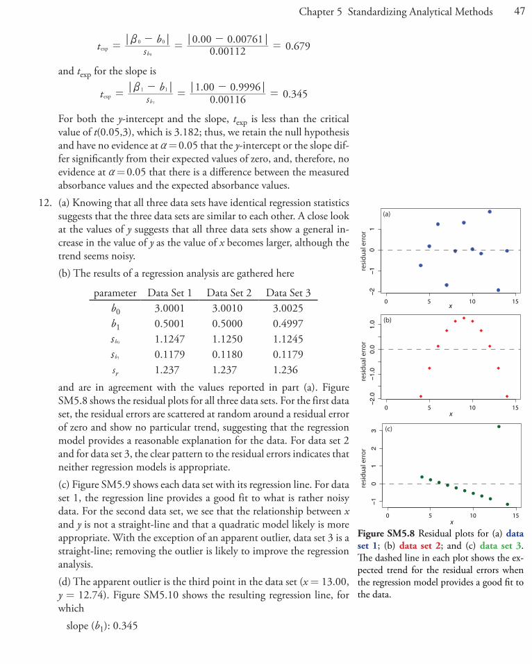
12. (a) Knowing that all three data sets have identical regression statistics suggests that the three data sets are similar to each other. A close look at the values of y suggests that all three data sets show a general in-crease in the value of y as the value of x becomes larger, although the trend seems noisy.

(b) The results of a regression analysis are gathered here

parameter Data Set 1 Data Set 2 Data Set 3b0 3.0001 3.0010 3.0025b1 0.5001 0.5000 0.4997sb0 1.1247 1.1250 1.1245sb1 0.1179 0.1180 0.1179sr 1.237 1.237 1.236

and are in agreement with the values reported in part (a). Figure SM5.8 shows the residual plots for all three data sets. For the first data set, the residual errors are scattered at random around a residual error of zero and show no particular trend, suggesting that the regression model provides a reasonable explanation for the data. For data set 2 and for data set 3, the clear pattern to the residual errors indicates that neither regression models is appropriate.

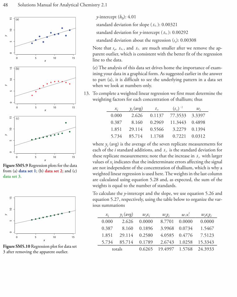
(c) Figure SM5.9 shows each data set with its regression line. For data set 1, the regression line provides a good fit to what is rather noisy data. For the second data set, we see that the relationship between x and y is not a straight-line and that a quadratic model likely is more appropriate. With the exception of an apparent outlier, data set 3 is a straight-line; removing the outlier is likely to improve the regression analysis.

(d) The apparent outlier is the third point in the data set (x = 13.00, y = 12.74). Figure SM5.10 shows the resulting regression line, for which

slope (b1): 0.345

0 5 10 15

−2−1

01

x

resi

dual

err

or

(a)

0 5 10 15

−2.0

−1.0

0.0

1.0

x

resi

dual

err

or

(b)

0 5 10 15

−10

12

3

x

resi

dual

err

or

(c)

Figure SM5.8 Residual plots for (a) data set 1; (b) data set 2; and (c) data set 3. The dashed line in each plot shows the ex-pected trend for the residual errors when the regression model provides a good fit to the data.

48 Solutions Manual for Analytical Chemistry 2.1

y-intercept (b0): 4.01 standard deviation for slope ( sb1 ): 0.00321 standard deviation for y-intercept ( sb0 ): 0.00292 standard deviation about the regression (sr): 0.00308 Note that sr, sb0 , and sb1 are much smaller after we remove the ap-

parent outlier, which is consistent with the better fit of the regression line to the data.

(e) The analysis of this data set drives home the importance of exam-ining your data in a graphical form. As suggested earlier in the answer to part (a), it is difficult to see the underlying pattern in a data set when we look at numbers only.

13. To complete a weighted linear regression we first must determine the weighting factors for each concentration of thallium; thus

xi yi (avg) s yi ( )s y2

i- wi

0.000 2.626 0.1137 77.3533 3.33970.387 8.160 0.2969 11.3443 0.48981.851 29.114 0.5566 3.2279 0.13945.734 85.714 1.1768 0.7221 0.0312

where yi (avg) is the average of the seven replicate measurements for each of the i standard additions, and s yi is the standard deviation for these replicate measurements; note that the increase in s yi with larger values of xi indicates that the indeterminate errors affecting the signal are not independent of the concentration of thallium, which is why a weighted linear regression is used here. The weights in the last column are calculated using equation 5.28 and, as expected, the sum of the weights is equal to the number of standards.

To calculate the y-intercept and the slope, we use equation 5.26 and equation 5.27, respectively, using the table below to organize the var-ious summations

xi yi (avg) wixi wiyi w xi i2 wixiyi

0.000 2.626 0.0000 8.7701 0.0000 0.00000.387 8.160 0.1896 3.9968 0.0734 1.54671.851 29.114 0.2580 4.0585 0.4776 7.51235.734 85.714 0.1789 2.6743 1.0258 15.3343

totals 0.6265 19.4997 1.5768 24.3933

0 5 10 15

05

1015

x

y

(a)

0 5 10 15

05

1015

x

y

(b)

0 5 10 15

05

1015

x

y

(c)

Figure SM5.9 Regression plots for the data from (a) data set 1; (b) data set 2; and (c) data set 3.

0 5 10 15

05

1015

x

y

Figure SM5.10 Regression plot for data set 3 after removing the apparent outlier.

49Chapter 5 Standardizing Analytical Methods

( ) ( . ) ( . )( ) ( . ) ( . ) ( . ) .

bn w x w x

n w x y w x w y

4 1 5768 0 62654 24 3933 0 6265 19 4997 14 43

i i i ii

n

i

n

i i i i ii

n

i ii

n

i

n

12

11

1 11

2

2=-

-

=-

-=

==

= ==

c m/// //

. ( . ) ( . ) .

b n

w b w xy

419 4997 14 431 0 6265 2 61

i ii

n

i ii

n

01

11=

-

=-

=

= =

/ /

The calibration curve, therefore, is. ( . )S C2 61 14 43µA µA/ppmtotal Tl#= +

Figure SM5.11 shows the calibration data and the weighted linear regression line.

Figure SM5.11 Calibration data and cali-bration curve for the data in Problem 5.13. The individual points show the average sig-nal for each standard and the calibration curve is from a weighted linear regression. The blue tick marks along the y-axis show the replicate signals for each standard; note that the spacing of these marks reflect the increased magnitude of the signal’s indeter-minate error for higher concentrations of thallium.

0 1 2 3 4 5 6

020

4060

8010

0

S tota

l

CTl

50 Solutions Manual for Analytical Chemistry 2.1