Chapter Thirteen1 CHAPTER THIRTEEN Aggregate Supply.

Chapter Thirteen

1

CHAPTER THIRTEENAggregate Supply

Chapter Thirteen

2

Chapter 9 - aggregate supply behaves differently in the short run than in the long run.

In the long run, prices are flexible, and the aggregate supply curve is vertical. When the aggregate supply curve is vertical, shifts in the aggregate demand curve affect the price level, but the output of the economy remains at its natural rate.

In the short run, prices are sticky, and the aggregate supply curve is not vertical. In this case, shifts in aggregate demand do cause fluctuations in output. In chapter 9, we took a simplified view of price stickiness by drawing the short-run aggregate supply curve as a horizontal line, representing the extreme situation in which all prices are fixed.

So, now we’ll refine our understanding of short-run aggregate supply.

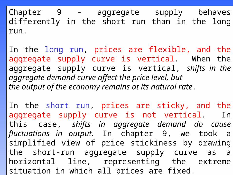
Chapter 9 - aggregate supply behaves differently in the short run than in the long run.

In the long run, prices are flexible, and the aggregate supply curve is vertical. When the aggregate supply curve is vertical, shifts in the aggregate demand curve affect the price level, but the output of the economy remains at its natural rate.

In the short run, prices are sticky, and the aggregate supply curve is not vertical. In this case, shifts in aggregate demand do cause fluctuations in output. In chapter 9, we took a simplified view of price stickiness by drawing the short-run aggregate supply curve as a horizontal line, representing the extreme situation in which all prices are fixed.

So, now we’ll refine our understanding of short-run aggregate supply.

Chapter Thirteen

3

In all the models, some market imperfection causes the output of the economy to deviate from its classical benchmark. As a result, the short-run aggregate supply curve is upward sloping, rather than vertical, and shifts in the aggregate demand curve cause the level of output to deviate temporarily from the natural rate. These temporary deviations represent the booms and busts of the business cycle.

Although each of the four models takes us down a different theoretical route, each route ends up in the same place. That final destination is a short-run aggregate supply equation of the form…

Chapter Thirteen

4

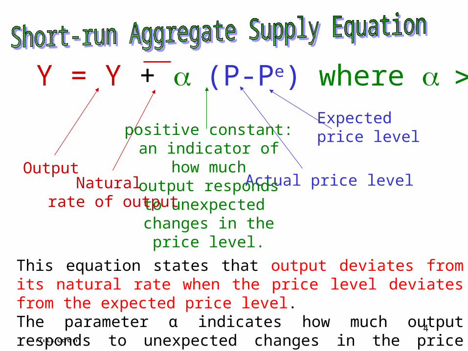
Y = Y + (P-Pe) where

OutputActual price level

positive constant:an indicator of

how muchoutput respondsto unexpected changes in the

price level.

Natural rate of output

Expected price level

This equation states that output deviates from its natural rate when the price level deviates from the expected price level. The parameter α indicates how much output responds to unexpected changes in the price level, 1/α is the slope of the aggregate supply curve.

Chapter Thirteen

5

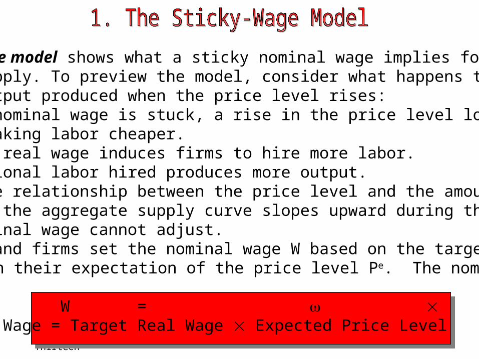
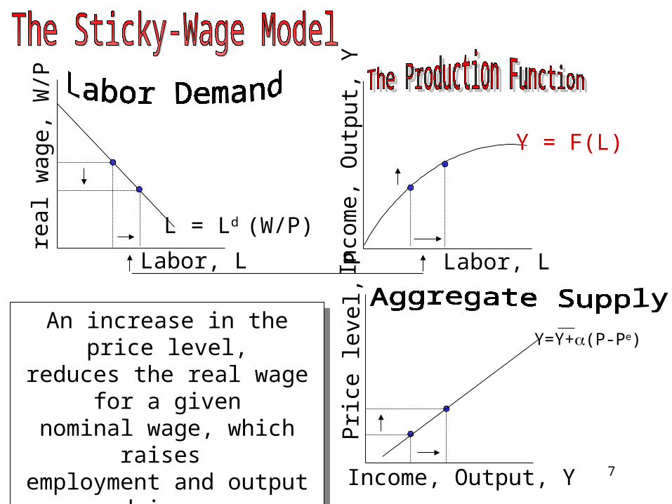
The sticky-wage model shows what a sticky nominal wage implies foraggregate supply. To preview the model, consider what happens to theamount of output produced when the price level rises:1) When the nominal wage is stuck, a rise in the price level lowers thereal wage, making labor cheaper.2) The lower real wage induces firms to hire more labor.3) The additional labor hired produces more output.This positive relationship between the price level and the amount of output means the aggregate supply curve slopes upward during the timewhen the nominal wage cannot adjust.The workers and firms set the nominal wage W based on the target realwage and on their expectation of the price level Pe. The nominal wagethey set is:

W = Pe

Nominal Wage = Target Real Wage Expected Price Level

Chapter Thirteen

6

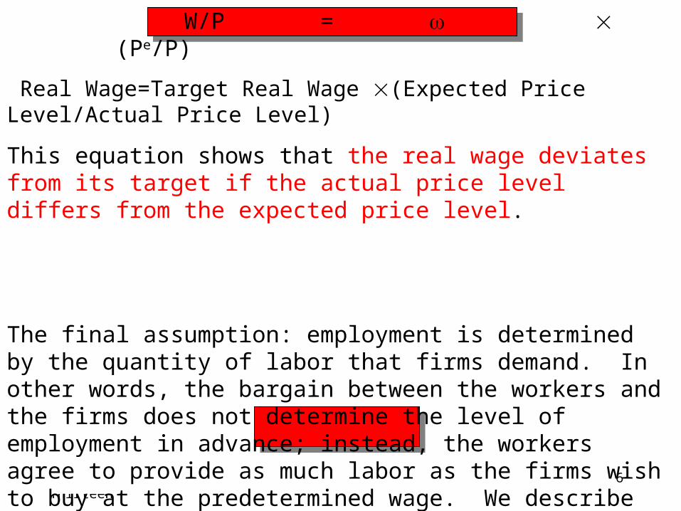
W/P = (Pe/P)

Real Wage=Target Real Wage (Expected Price Level/Actual Price Level)

This equation shows that the real wage deviates from its target if the actual price level differs from the expected price level.

The final assumption: employment is determined by the quantity of labor that firms demand. In other words, the bargain between the workers and the firms does not determine the level of employment in advance; instead, the workers agree to provide as much labor as the firms wish to buy at the predetermined wage. We describe the firms’ hiring decisions by the labor demand function:

L = Ld (W/P),

which states that the lower the real wage, the more labor firms hire and output is determined by the production function Y = F(L).

Chapter Thirteen

7

Labor, L

Y = F(L)

Income, Output, Y

Labor, L

L = Ld (W/P)

Y=Y+(P-Pe)

real

wag

e, W

/P

Inco

me,

Out

put,

YP

rice

leve

l, P

An increase in the price level,reduces the real wage for a given

nominal wage, which raises employment and output and

income.

An increase in the price level,reduces the real wage for a given

nominal wage, which raises employment and output and

income.

Chapter Thirteen

8

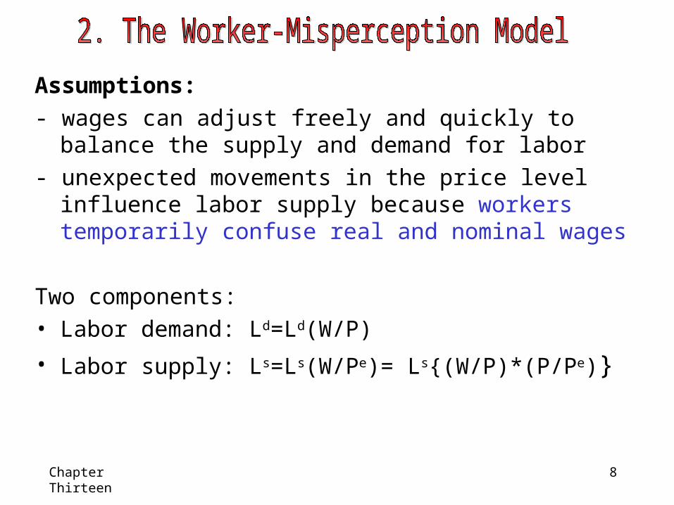
Assumptions:

- wages can adjust freely and quickly to balance the supply and demand for labor

- unexpected movements in the price level influence labor supply because workers temporarily confuse real and nominal wages

Two components:• Labor demand: Ld=Ld(W/P)

• Labor supply: Ls=Ls(W/Pe)= Ls{(W/P)*(P/Pe)}

Chapter Thirteen

9

Ld

L1s

L2s

Real w

age W/P

Labor, L

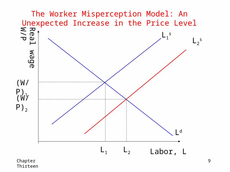
The Worker Misperception Model: An Unexpected Increase in the Price Level

L1 L2

(W/P)1

(W/P)2

Chapter Thirteen

10

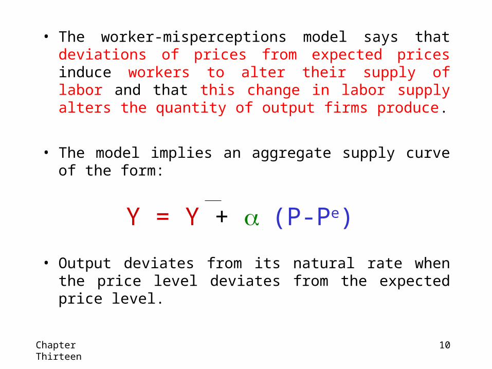
• The worker-misperceptions model says that deviations of prices from expected prices induce workers to alter their supply of labor and that this change in labor supply alters the quantity of output firms produce.

• The model implies an aggregate supply curve of the form:

• Output deviates from its natural rate when the price level deviates from the expected price level.

Y = Y + (P-Pe)

Chapter Thirteen

11

Unlike the sticky-wage model, this model assumes that markets clear-- that is, all wages and prices are free to adjust to balance supply and demand. In this model, the short-run and long-run aggregate supply curves differ because of temporary misperceptions about prices.The imperfect-information model assumes that each supplier in the economy produces a single good and consumes many goods. Because the number of goods is so large, suppliers cannot observe all prices at all times. They monitor the prices of their own goods but not the prices of all goods they consume. Due to imperfect information, they sometimes confuse changes in the overall price level with changes in relative prices.This confusion influences decisions about how much to supply, and it leads to a positive relationship between the price level and output in the short run.

Chapter Thirteen

12

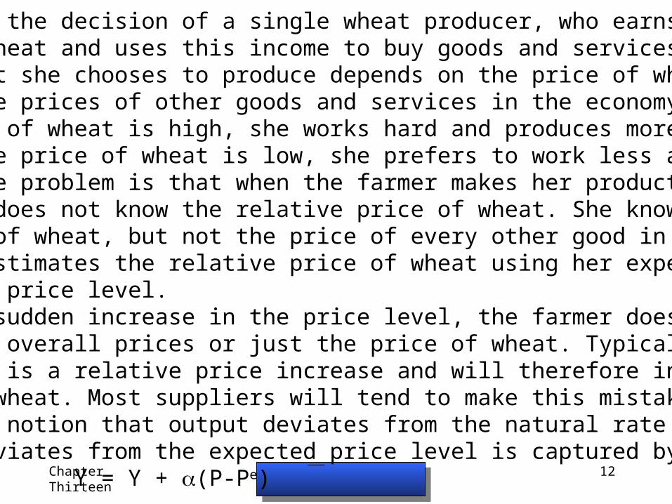
Let’s consider the decision of a single wheat producer, who earns incomefrom selling wheat and uses this income to buy goods and services. Theamount of wheat she chooses to produce depends on the price of wheatrelative to the prices of other goods and services in the economy. If the relative price of wheat is high, she works hard and produces more wheat.If the relative price of wheat is low, she prefers to work less and produceless wheat. The problem is that when the farmer makes her production decision, she does not know the relative price of wheat. She knows the nominal price of wheat, but not the price of every other good in the economy. She estimates the relative price of wheat using her expectations of the overall price level.If there is a sudden increase in the price level, the farmer doesn’t know if itis a change in overall prices or just the price of wheat. Typically, she will assume that it is a relative price increase and will therefore increase theproduction of wheat. Most suppliers will tend to make this mistake.To sum up, the notion that output deviates from the natural rate when theprice level deviates from the expected price level is captured by:

Y = Y + (P-Pe)

Chapter Thirteen

13

This model emphasizes that firms do not instantly adjust the prices they charge in response to changes in demand. Sometimes prices are set by long-term contracts between firms and consumers.

To see how sticky prices can help explain an upward-sloping aggregate supply curve, first consider the pricing decisions of individual firms and then aggregate the decisions of many firms to explain the economy as a whole. We will have to relax the assumption of perfect competition, whereby firms are price takers. Now they will be price setters.

Chapter Thirteen

14

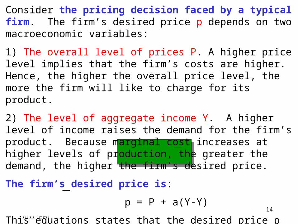
Consider the pricing decision faced by a typical firm. The firm’s desired price p depends on two macroeconomic variables:

1) The overall level of prices P. A higher price level implies that the firm’s costs are higher. Hence, the higher the overall price level, the more the firm will like to charge for its product.

2) The level of aggregate income Y. A higher level of income raises the demand for the firm’s product. Because marginal cost increases at higher levels of production, the greater the demand, the higher the firm’s desired price.

The firm’s desired price is:

p = P + a(Y-Y)

This equations states that the desired price p depends on the overall level of prices P and on the level of aggregate demand relative to its natural rate Y-Y. The parameter a (which is greater than 0) measures how much the firm’s desired price responds to the level of aggregate output.

Chapter Thirteen

15

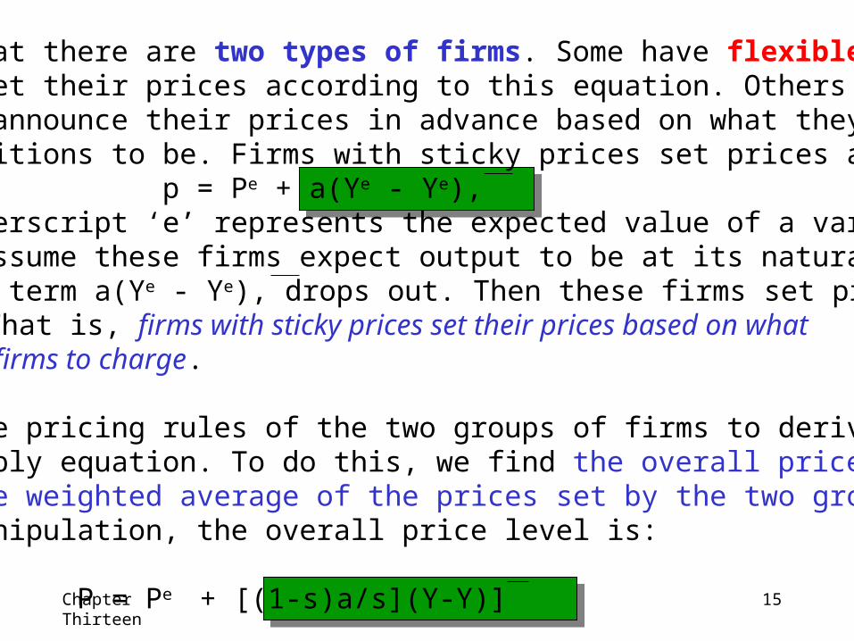
Now assume that there are two types of firms. Some have flexible prices:they always set their prices according to this equation. Others have stickyprices: they announce their prices in advance based on what they expect economic conditions to be. Firms with sticky prices set prices according to

p = Pe + a(Ye - Ye),where the superscript ‘e’ represents the expected value of a variable. Forsimplicity, assume these firms expect output to be at its natural rate so that the last term a(Ye - Ye), drops out. Then these firms set price sothat p = Pe. That is, firms with sticky prices set their prices based on whatthey expect other firms to charge.

We can use the pricing rules of the two groups of firms to derive theaggregate supply equation. To do this, we find the overall price level in theeconomy as the weighted average of the prices set by the two groups.After some manipulation, the overall price level is:

P = Pe + [(1-s)a/s](Y-Y)]

Chapter Thirteen

16

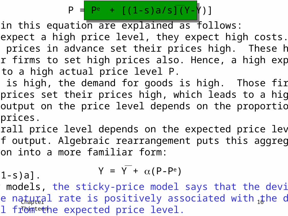
P = Pe + [(1-s)a/s](Y-Y)]

The two terms in this equation are explained as follows:1) When firms expect a high price level, they expect high costs. Thosefirms that fix prices in advance set their prices high. These high pricescause the other firms to set high prices also. Hence, a high expected pricelevel Pe leads to a high actual price level P.2) When output is high, the demand for goods is high. Those firmswith flexible prices set their prices high, which leads to a high price level.The effect of output on the price level depends on the proportion of firmswith flexible prices. Hence, the overall price level depends on the expected price level and on the level of output. Algebraic rearrangement puts this aggregate pricing equation into a more familiar form:

where = s/[(1-s)a]. Like the other models, the sticky-price model says that the deviation of output from the natural rate is positively associated with the deviation of the price level from the expected price level.

Y = Y + (P-Pe)

Chapter Thirteen

17

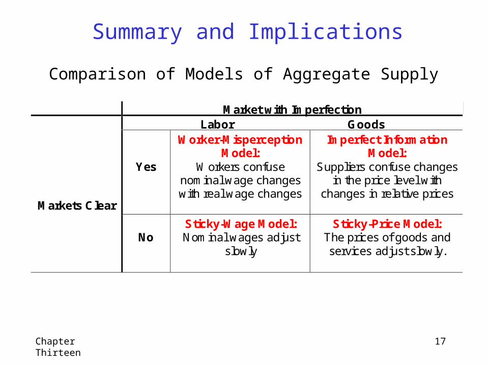
Summary and Implications

Comparison of Models of Aggregate Supply

Market with ImperfectionLabor Goods

Yes

Worker-MisperceptionModel:

Workers confusenominal wage changeswith real wage changes

Imperfect InformationModel:

Suppliers confuse changesin the price level with

changes in relative pricesMarkets Clear

NoSticky-Wage Model:Nominal wages adjust

slowly

Sticky-Price Model:The prices of goods andservices adjust slowly.

Chapter Thirteen

18

The 4 models of aggregate supply differ in two characteristics:

• whether they assume that markets clear

• whether the key market imperfection lies in the goods market or in the labor market

Chapter Thirteen

19

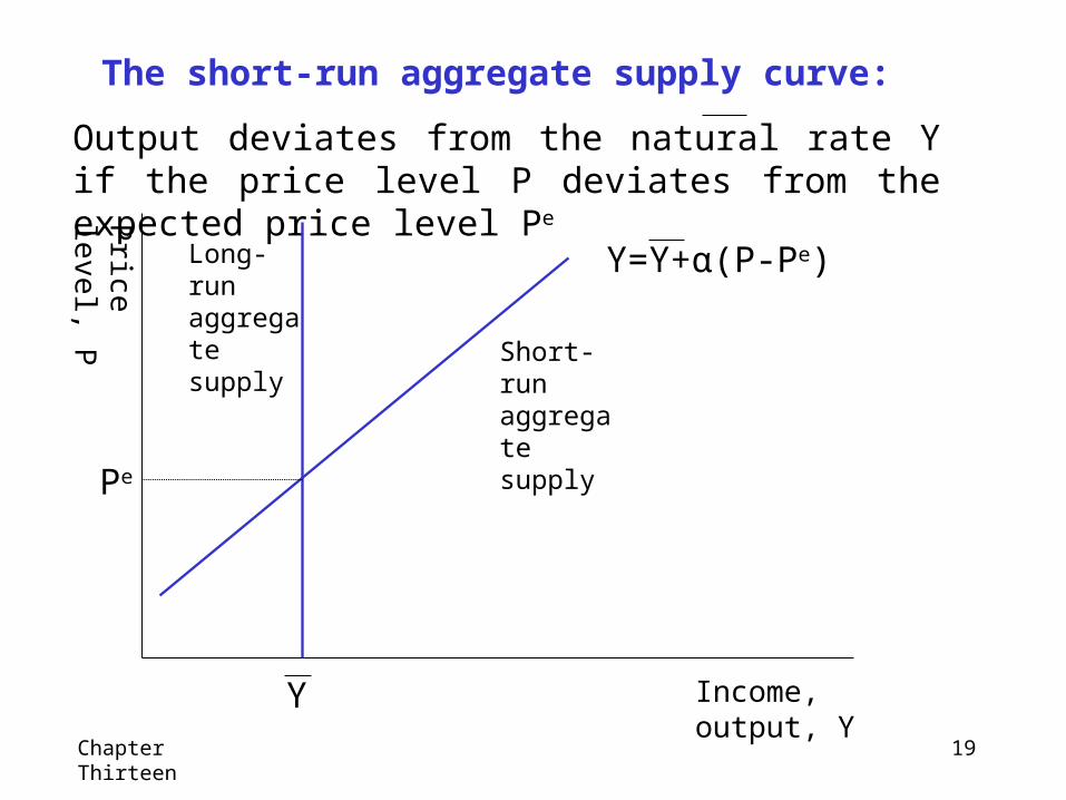
The short-run aggregate supply curve:

Output deviates from the natural rate Y if the price level P deviates from the expected price level Pe

Price

level, P

Income, output, Y

Pe

Y

Long-run aggregate supply

Short-run aggregate supply

Y=Y+α(P-Pe)

Chapter Thirteen

20

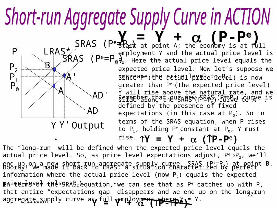
Start at point A; the economy is at full employment Y and the actual price level is P0. Here the actual price level equals the expected price level. Now let’s suppose we increase the price level to P1.

Since P (the actual price level) is now greater than Pe (the expected price level) Y will rise above the natural rate, and we slide along the SRAS (Pe=P0) curve to A' . Remember that our new SRAS (Pe=P0) curve is defined by the presence of fixed expectations (in this case at P0). So in terms of the SRAS equation, when P rises to P1, holding Pe constant at P0, Y must rise.

The “long-run” will be defined when the expected price level equals the actual price level. So, as price level expectations adjust, PeP2, we’ll end up on a new short-run aggregate supply curve, SRAS (Pe=P2) at point B.

Hooray! We made it back to LRAS, a situation characterized by perfect information where the actual price level (now P2) equals the expected price level (also, P2).

Y = Y + (P-Pe)

Y = Y + (P-Pe)

Y = Y + (P-Pe)

In terms of the SRAS equation, we can see that as Pe catches up with P, that entire “expectations gap” disappears and we end up on the long run aggregate supply curve at full employment where Y = Y.

SRAS (Pe=P2)

BP2

A'

Y'

SRAS (Pe=P0)P

Output

AP0

LRAS*

Y

AD

AD'

P1

Chapter Thirteen

21

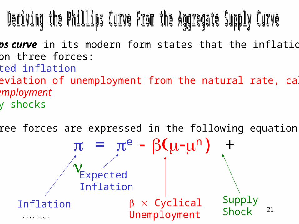
The Phillips curve in its modern form states that the inflation ratedepends on three forces:1) Expected inflation2) The deviation of unemployment from the natural rate, called cyclical unemployment3) Supply shocks

These three forces are expressed in the following equation:

= e n) +

Inflation Cyclical Unemployment

Supply Shock

Expected Inflation

Chapter Thirteen

22

The Phillips-curve equation and the short-run aggregate supply equation represent essentially the same macroeconomic ideas.

Both equations show a link between real and nominal variables that causes the classical dichotomy (the theoretical separation of real and nominal variables) to break down in the short run.

The Phillips curve and the aggregate supply curve are two sides of the same coin. The aggregate supply curve is more convenient when studying output and the price level, whereas the Phillips curve is more convenient when studying unemployment and inflation.

Chapter Thirteen

23

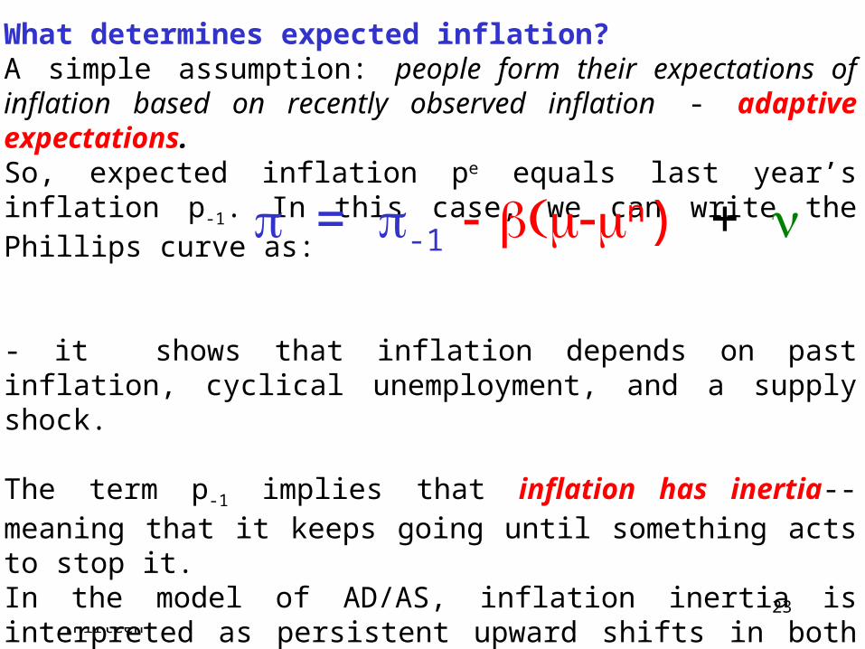
What determines expected inflation? A simple assumption: people form their expectations of inflation based on recently observed inflation - adaptive expectations. So, expected inflation pe equals last year’s inflation p-1. In this case, we can write the Phillips curve as:

- it shows that inflation depends on past inflation, cyclical unemployment, and a supply shock.

The term p-1 implies that inflation has inertia-- meaning that it keeps going until something acts to stop it. In the model of AD/AS, inflation inertia is interpreted as persistent upward shifts in both the aggregate supply curve and aggregate demand curve. Because the position of the SRAS will shift upwards overtime, it will continue to shift upward until something changes inflation expectations.

= -1 n) +

Chapter Thirteen

24

• Robert Solow, during the high inflation of 1970s, wrote: “Why is our money less valuable? Perhaps it is simply that we have inflation because we expect inflation, and we expect inflation because we’ve had it.”

Chapter Thirteen

25

Let’s look at the second and third terms in the Phillips-curve equation: the two forces that can change the rate of inflation. •The second term, β(u-un) - shows that cyclical unemployment exerts downward pressure on inflation. Low unemployment pulls the inflation rate up - demand-pull inflation (because high aggregate demand is responsible for this type of inflation). High unemployment pulls the inflation rate down. The parameter β measures how responsive inflation is to cyclical unemployment.

•The third term, ν- shows that inflation also rises and falls because of supply shocks. An adverse supply shock, such as the rise in world oil prices in the 70’s, implies a positive value of n and causes inflation to rise - cost-push inflation (because adverse supply shocks are typically events that push up the costs of production).

Chapter Thirteen

26

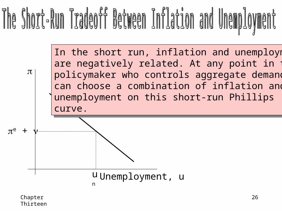
un

Unemployment, u

e +

In the short run, inflation and unemploymentare negatively related. At any point in time, apolicymaker who controls aggregate demandcan choose a combination of inflation andunemployment on this short-run Phillipscurve.

In the short run, inflation and unemploymentare negatively related. At any point in time, apolicymaker who controls aggregate demandcan choose a combination of inflation andunemployment on this short-run Phillipscurve.

Chapter Thirteen

27

Rational expectations make the assumption that people optimally use all the available information about current government policies, to forecast the future.

•According to this theory, a change in monetary or fiscal policy will change expectations, and an evaluation of any policy change must incorporate this effect on expectations.

•If people do form their expectations rationally, then inflation may have less inertia than it first appears.

Chapter Thirteen

28

• Proponents of rational expectations argue that the short-run Phillips curve does not accurately represent the options that policymakers have available.

• They believe that if policy makers are credibly committed to reducing inflation, rational people will understand the commitment and lower their expectations of inflation. Inflation can then come down without a rise in unemployment and fall in output.

Chapter Thirteen

29

Our entire discussion has been based on the natural rate hypothesis.The hypothesis is summarized in the following statement:

Fluctuations in aggregate demand affect output and employment only in the short run. In the long run, the economy returns to the levels of output,employment, and unemployment described by the classical model.

Recently, some economists have challenged the natural-rate hypothesisby suggesting that aggregate demand may affect output and employmenteven in the long run. They have pointed out a number of mechanismsthrough which recessions might leave permanent scars on the economyby altering the natural rate of unemployment. Hyteresis is the termused to describe the long-lasting influence of history on the naturalrate.

Chapter Thirteen

30

Conclusions

Four models of aggregate supply:• each focuses on a different reason why the short-run

aggregate supply curve is upward sloping• they have similar predictions• all of them yield a short-run tradeoff between inflation

and unemployment

The tradeoff between inflation and unemployment is called the Phillips curve: inflation depends on expected inflation, cyclical unemployment and supply shocks.

Chapter Thirteen

31

Sticky-wage modelImperfect-information modelSticky-price modelPhillips curveAdaptive expectationsDemand-pull inflationCost-push inflationSacrifice ratioRational expectationsNatural-rate hypothesisHyteresis

Sticky-wage modelImperfect-information modelSticky-price modelPhillips curveAdaptive expectationsDemand-pull inflationCost-push inflationSacrifice ratioRational expectationsNatural-rate hypothesisHyteresis