411 Chapter 9 Titrimetric Methods Chapter Overview Section 9A Overview of Titrimetry Section 9B Acid–Base Titrations Section 9C Complexation Titrations Section 9D Redox Titrations Section 9E Precipitation Titrations Section 9F Key Terms Section 9G Chapter Summary Section 9H Problems Section 9I Solutions to Practice Exercises Titrimetry, in which volume serves as the analytical signal, made its first appearance as an analytical method in the early eighteenth century. Titrimetric methods were not well received by the analytical chemists of that era because they could not duplicate the accuracy and precision of a gravimetric analysis. Not surprisingly, few standard texts from the 1700s and 1800s include titrimetric methods of analysis. Precipitation gravimetry developed as an analytical method without a general theory of precipitation. An empirical relationship between a precipitate’s mass and the mass of analyte— what analytical chemists call a gravimetric factor—was determined experimentally by taking a known mass of analyte through the procedure. Today, we recognize this as an early example of an external standardization. Gravimetric factors were not calculated using the stoichiometry of a precipitation reaction because chemical formulas and atomic weights were not yet available! Unlike gravimetry, the development and acceptance of titrimetry required a deeper understanding of stoichiometry, of thermodynamics, and of chemical equilibria. By the 1900s, the accuracy and precision of titrimetric methods were comparable to that of gravimetric methods, establishing titrimetry as an accepted analytical technique.

Welcome message from author
This document is posted to help you gain knowledge. Please leave a comment to let me know what you think about it! Share it to your friends and learn new things together.
Transcript

411
Chapter 9
Titrimetric MethodsChapter OverviewSection 9A Overview of TitrimetrySection 9B Acid–Base TitrationsSection 9C Complexation TitrationsSection 9D Redox TitrationsSection 9E Precipitation TitrationsSection 9F Key TermsSection 9G Chapter SummarySection 9H ProblemsSection 9I Solutions to Practice Exercises
Titrimetry, in which volume serves as the analytical signal, made its first appearance as an analytical method in the early eighteenth century. Titrimetric methods were not well received by the analytical chemists of that era because they could not duplicate the accuracy and precision of a gravimetric analysis. Not surprisingly, few standard texts from the 1700s and 1800s include titrimetric methods of analysis.
Precipitation gravimetry developed as an analytical method without a general theory of precipitation. An empirical relationship between a precipitate’s mass and the mass of analyte—what analytical chemists call a gravimetric factor—was determined experimentally by taking a known mass of analyte through the procedure. Today, we recognize this as an early example of an external standardization. Gravimetric factors were not calculated using the stoichiometry of a precipitation reaction because chemical formulas and atomic weights were not yet available! Unlike gravimetry, the development and acceptance of titrimetry required a deeper understanding of stoichiometry, of thermodynamics, and of chemical equilibria. By the 1900s, the accuracy and precision of titrimetric methods were comparable to that of gravimetric methods, establishing titrimetry as an accepted analytical technique.

412 Analytical Chemistry 2.0
9A Overview of TitrimetryIn titrimetry we add a reagent, called the titrant, to a solution contain-ing another reagent, called the titrand, and allow them to react. The type of reaction provides us with a simple way to divide titrimetry into the following four categories: acid–base titrations, in which an acidic or basic titrant reacts with a titrand that is a base or an acid; complexometric titra-tions based on metal–ligand complexation; redox titrations, in which the titrant is an oxidizing or reducing agent; and precipitation titrations, in which the titrand and titrant form a precipitate.
Despite the difference in chemistry, all titrations share several com-mon features. Before we consider individual titrimetric methods in greater detail, let’s take a moment to consider some of these similarities. As you work through this chapter, this overview will help you focus on similarities between different titrimetric methods. You will find it easier to understand a new analytical method when you can see its relationship to other similar methods.
9A.1 Equivalence Points and End points
If a titration is to be accurate we must combine stoichiometrically equiva-lent amount of titrant and titrand. We call this stoichiometric mixture the equivalence point. Unlike precipitation gravimetry, where we add the precipitant in excess, an accurate titration requires that we know the exact volume of titrant at the equivalence point, Veq. The product of the titrant’s equivalence point volume and its molarity, MT, is equal to the moles of titrant reacting with the titrand.
moles of titrant T eq= �M V
If we know the stoichiometry of the titration reaction, then we can calculate the moles of titrand.
Unfortunately, for most titrations there is no obvious sign when we reach the equivalence point. Instead, we stop adding titrant when at an end point of our choosing. Often this end point is a change in the color of a substance, called an indicator, that we add to the titrand’s solution. The difference between the end point volume and the equivalence point volume is a determinate titration error. If the end point and the equivalence point volumes coincide closely, then the titration error is insignificant and it is safely ignored. Clearly, selecting an appropriate end point is critically important.
9A.2 Volume as a Signal
Almost any chemical reaction can serve as a titrimetric method provided it meets the following four conditions. The first condition is that we must know the stoichiometry between the titrant and the titrand. If this is not
We are deliberately avoiding the term analyte at this point in our introduction to titrimetry. Although in most titrations the analyte is the titrand, there are circum-stances where the analyte is the titrant. When discussing specific methods, we will use the term analyte where appropriate.
Instead of measuring the titrant’s volume, we may choose to measure its mass. Al-though we generally can measure mass more precisely than we can measure vol-ume, the simplicity of a volumetric titra-tion makes it the more popular choice.

413Chapter 9 Titrimetric Methods
the case, then we cannot convert the moles of titrant consumed in reaching the end point to the moles of titrand in our sample. Second, the titration reaction must effectively proceed to completion; that is, the stoichiometric mixing of the titrant and the titrand must result in their reaction. Third, the titration reaction must occur rapidly. If we add the titrant faster than it can react with the titrand, then the end point and the equivalence point will differ significantly. Finally, there must be a suitable method for accurately determining the end point. These are significant limitations and, for this reason, there are several common titration strategies.
A simple example of a titration is an analysis for Ag+ using thiocyanate, SCN–, as a titrant.
Ag SCN Ag(SCN)+ −+( ) ( ) ( )aq aq s
This reaction occurs quickly and with a known stoichiometry, satisfying two of our requirements. To indicate the titration’s end point, we add a small amount of Fe3+ to the analyte’s solution before beginning the titration. When the reaction between Ag+ and SCN– is complete, formation of the red-colored Fe(SCN)2+ complex signals the end point. This is an example of a direct titration since the titrant reacts directly with the analyte.
If the titration’s reaction is too slow, if a suitable indicator is not avail-able, or if there is no useful direct titration reaction, then an indirect analy-sis may be possible. Suppose you wish to determine the concentration of formaldehyde, H2CO, in an aqueous solution. The oxidation of H2CO by I3
–
H CO I OH HCO I2 ( ) ( ) ( ) ( ) ( )aq aq aq aq aq+ + +− − − −3 23 3 ++ 2H O2 ( )l
is a useful reaction, but it is too slow for a titration. If we add a known excess of I3
– and allow its reaction with H2CO to go to completion, we can titrate the unreacted I3
– with thiosulfate, S2O32–.
I S O S O I2 43 32
622 3− − − −+ +( ) ( ) ( ) ( )aq aq aq aq
The difference between the initial amount of I3– and the amount in excess
gives us the amount of I3– reacting with the formaldehyde. This is an ex-
ample of a back titration.Calcium ion plays an important role in many environmental systems. A
direct analysis for Ca2+ might take advantage of its reaction with the ligand ethylenediaminetetraacetic acid (EDTA), which we represent here as Y4–.
Ca Y CaY2 4 2+ − −+( ) ( ) ( )aq aq aq
Unfortunately, for most samples this titration does not have a useful indica-tor. Instead, we react the Ca2+ with an excess of MgY2–
Ca MgY CaY Mg2 2 2 2+ − − ++ +( ) ( ) ( ) ( )aq aq aq aq
Depending on how we are detecting the endpoint, we may stop the titration too early or too late. If the end point is a func-tion of the titrant’s concentration, then adding the titrant too quickly leads to an early end point. On the other hand, if the end point is a function of the titrant’s con-centration, then the end point exceeds the equivalence point.
This is an example of a precipitation titra-tion. You will find more information about precipitation titrations in Section 9E.
This is an example of a redox titration. You will find more information about redox titrations in Section 9D.
MgY2– is the Mg2+–EDTA metal–ligand complex. You can prepare a solution of MgY2– by combining equimolar solu-tions of Mg2+ and EDTA.

414 Analytical Chemistry 2.0
releasing an amount of Mg2+ equivalent to the amount of Ca2+ in the sample. Because the titration of Mg2+ with EDTA
Mg Y Y2 4 2+ − −+( ) ( ) ( )aq aq aqMg
has a suitable end point, we can complete the analysis. The amount of EDTA used in the titration provides an indirect measure of the amount of Ca2+ in the original sample. Because the species we are titrating was dis-placed by the analyte, we call this a displacement titration.
If a suitable reaction involving the analyte does not exist it may be pos-sible to generate a species that we can titrate. For example, we can deter-mine the sulfur content of coal by using a combustion reaction to convert sulfur to sulfur dioxide
S O SO( ) ( ) ( )s g g+ →2 2
and then convert the SO2 to sulfuric acid, H2SO4, by bubbling it through an aqueous solution of hydrogen peroxide, H2O2.
SO H O H SO2 2 2 42( ) ( ) ( )g aq aq+ →
Titrating H2SO4 with NaOH
H SO NaOH H O Na SO2 4 2 2 4( ) ( ) ( ) ( )aq aq l aq+ +2 2
provides an indirect determination of sulfur.
9A.3 Titration Curves
To find a titration’s end point, we need to monitor some property of the reaction that has a well-defined value at the equivalence point. For example, the equivalence point for a titration of HCl with NaOH occurs at a pH of 7.0. A simple method for finding the equivalence point is to continuously monitor the titration mixture’s pH using a pH electrode, stopping the titra-tion when we reach a pH of 7.0. Alternatively, we can add an indicator to the titrand’s solution that changes color at a pH of 7.0.
Suppose the only available indicator changes color at an end point pH of 6.8. Is the difference between the end point and the equivalence point small enough that we can safely ignore the titration error? To answer this question we need to know how the pH changes during the titration.
A titration curve provides us with a visual picture of how a property of the titration reaction changes as we add the titrant to the titrand. The titration curve in Figure 9.1, for example, was obtained by suspending a pH electrode in a solution of 0.100 M HCl (the titrand) and monitoring the pH while adding 0.100 M NaOH (the titrant). A close examination of this titration curve should convince you that an end point pH of 6.8 produces a negligible titration error. Selecting a pH of 11.6 as the end point, however, produces an unacceptably large titration error.
This is an example of an acid–base titra-tion. You will find more information about acid–base titrations in Section 9B.
For the titration curve in Figure 9.1, the volume of titrant to reach a pH of 6.8 is 24.99995 mL, a titration error of –2.00�10–4%. Typically, we can only read the volume to the nearest ±0.01 mL, which means this uncertainty is too small to affect our results.
The volume of titrant to reach a pH of 11.6 is 27.07 mL, or a titration error of +8.28%. This is a significant error.
This is an example of a complexation titration. You will find more information about complexation titrations in Section 9C.
Why a pH of 7.0 is the equivalence point for this titration is a topic we will cover in Section 9B.

415Chapter 9 Titrimetric Methods
The titration curve in Figure 9.1 is not unique to an acid–base titration. Any titration curve that follows the change in concentration of a species in the titration reaction (plotted logarithmically) as a function of the titrant’s volume has the same general sigmoidal shape. Several additional examples are shown in Figure 9.2.
The titrand’s or the titrant’s concentration is not the only property we can use when recording a titration curve. Other parameters, such as the temperature or absorbance of the titrand’s solution, may provide a use-ful end point signal. Many acid–base titration reactions, for example, are exothermic. As the titrant and titrand react the temperature of the titrand’s solution steadily increases. Once we reach the equivalence point, further additions of titrant do not produce as exothermic a response. Figure 9.3 shows a typical thermometric titration curve with the intersection of the two linear segments indicating the equivalence point.
Figure 9.1 Typical acid–base titration curve showing how the titrand’s pH changes with the addition of titrant. The titrand is a 25.0 mL solution of 0.100 M HCl and the titrant is 0.100 M NaOH. The titration curve is the solid blue line, and the equivalence point volume (25.0 mL) and pH (7.00) are shown by the dashed red lines. The green dots show two end points. The end point at a pH of 6.8 has a small titra-tion error, and the end point at a pH of 11.6 has a larger titration error.
0 10 20 30 40 50VEDTA (mL) VCe4+ (mL) VAgNO3 (mL)
pCd
E (V
)
pAg
0
5
10
15
0 10 20 30 40 500.6
0.81.0
1.2
1.41.6
0 10 20 30 40 50
2
4
6
8
10(a) (b) (c)
Figure 9.2 Additional examples of titration curves. (a) Complexation titration of 25.0 mL of 1.0 mM Cd2+ with 1.0 mM EDTA at a pH of 10. The y-axis displays the titrand’s equilibrium concentration as pCd. (b) Redox titration of 25.0 mL of 0.050 M Fe2+ with 0.050 M Ce4+ in 1 M HClO4. The y-axis displays the titration mixture’s electrochemical potential, E, which, through the Nernst equation is a logarithmic function of concentrations. (c) Precipitation titration of 25.0 mL of 0.10 M NaCl with 0.10 M AgNO3. The y-axis displays the titrant’s equilibrium concentration as pAg.
0 10 20 30 40 50
2
4
6
8
10
12
14pH
VNaOH (mL)
pH at Veq = 7.00
Veq = 25.0 mL
end pointpH of 6.8
end pointpH of 11.6

416 Analytical Chemistry 2.0
9A.4 The Buret
The only essential equipment for an acid–base titration is a means for de-livering the titrant to the titrand’s solution. The most common method for delivering titrant is a buret (Figure 9.4). A buret is a long, narrow tube with graduated markings, equipped with a stopcock for dispensing the titrant. The buret’s small internal diameter provides a better defined meniscus, mak-ing it easier to read the titrant’s volume precisely. Burets are available in a variety of sizes and tolerances (Table 9.1), with the choice of buret deter-mined by the needs of the analysis. You can improve a buret’s accuracy by calibrating it over several intermediate ranges of volumes using the method described in Chapter 5 for calibrating pipets. Calibrating a buret corrects for variations in the buret’s internal diameter.
A titration can be automated by using a pump to deliver the titrant at a constant flow rate (Figure 9.5). Automated titrations offer the additional advantage of using a microcomputer for data storage and analysis.
Figure 9.3 Example of a thermometric titration curve showing the location of the equivalence point.
Figure 9.4 Typical volumetric bu-ret. The stopcock is in the open position, allowing the titrant to flow into the titrand’s solution. Rotating the stopcock controls the titrant’s flow rate.
Table 9.1 Specifications for Volumetric BuretsVolume (mL) Class Subdivision (mL) Tolerance (mL)
5 AB
0.010.01
±0.01±0.01
10 AB
0.020.02
±0.02±0.04
25 AB
0.10.1
±0.03±0.06
50 AB
0.10.1
±0.05±0.10
100 AB
0.20.2
±0.10±0.20
Tem
pera
ture
(o C)
Volume of titrant (mL)
equivalencepoint
stopcock

417Chapter 9 Titrimetric Methods
9B Acid–Base TitrationsBefore 1800, most acid–base titrations used H2SO4, HCl, or HNO3 as acidic titrants, and K2CO3 or Na2CO3 as basic titrants. A titration’s end point was determined using litmus as an indicator, which is red in acidic solutions and blue in basic solutions, or by the cessation of CO2 efferves-cence when neutralizing CO3
2–. Early examples of acid–base titrimetry include determining the acidity or alkalinity of solutions, and determining the purity of carbonates and alkaline earth oxides.
Three limitations slowed the development of acid–base titrimetry: the lack of a strong base titrant for the analysis of weak acids, the lack of suit-able indicators, and the absence of a theory of acid–base reactivity. The introduction, in 1846, of NaOH as a strong base titrant extended acid–base titrimetry to the determination of weak acids. The synthesis of organic dyes provided many new indicators. Phenolphthalein, for example, was first synthesized by Bayer in 1871 and used as an indicator for acid–base titrations in 1877.
Despite the increasing availability of indicators, the absence of a theory of acid–base reactivity made it difficult to select an indicator. The devel-opment of equilibrium theory in the late 19th century led to significant improvements in the theoretical understanding of acid–base chemistry, and, in turn, of acid–base titrimetry. Sørenson’s establishment of the pH scale in 1909 provided a rigorous means for comparing indicators. The deter-mination of acid–base dissociation constants made it possible to calculate a theoretical titration curve, as outlined by Bjerrum in 1914. For the first
Figure 9.5 Typical instrumentation for an automated acid–base titration showing the titrant, the pump, and the titrand. The pH electrode in the titrand’s solution is used to monitor the titration’s progress. You can see the titration curve in the lower-left quadrant of the computer’s display. Modified from: Datamax (commons.wikipedia.org).
The determination of acidity and alkalin-ity continue to be important applications of acid–base titrimetry. We will take a closer look at these applications later in this section.
titrant
titrand
pump
418 Analytical Chemistry 2.0
time analytical chemists had a rational method for selecting an indicator, establishing acid–base titrimetry as a useful alternative to gravimetry.
9B.1 Acid–Base Titration Curves
In the overview to this chapter we noted that a titration’s end point should coincide with its equivalence point. To understand the relationship between an acid–base titration’s end point and its equivalence point we must know how the pH changes during a titration. In this section we will learn how to calculate a titration curve using the equilibrium calculations from Chapter 6. We also will learn how to quickly sketch a good approximation of any acid–base titration curve using a limited number of simple calculations.
TiTraTing STrong acidS and STrong BaSeS
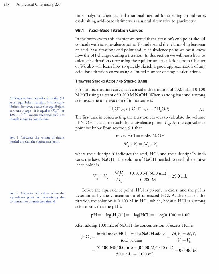
For our first titration curve, let’s consider the titration of 50.0 mL of 0.100 M HCl using a titrant of 0.200 M NaOH. When a strong base and a strong acid react the only reaction of importance is
H O OH H O3 2+ −+ →( ) ( ) ( )aq aq l2 9.1
The first task in constructing the titration curve is to calculate the volume of NaOH needed to reach the equivalence point, Veq. At the equivalence point we know from reaction 9.1 that
moles HCl = moles NaOH
M V M Va a b b� = �
where the subscript ‘a’ indicates the acid, HCl, and the subscript ‘b’ indi-cates the base, NaOH. The volume of NaOH needed to reach the equiva-lence point is
V VM VMeq b
a a
b
M)(50.0 mL)M
= = = =( .
..
0 1000 200
25 00 mL
Before the equivalence point, HCl is present in excess and the pH is determined by the concentration of unreacted HCl. At the start of the titration the solution is 0.100 M in HCl, which, because HCl is a strong acid, means that the pH is
pH H O HCl3=− =− =− =+log[ ] log[ ] log( . ) .0 100 1 00
After adding 10.0 mL of NaOH the concentration of excess HCl is
[ ]HClinitial moles HCl moles NaOH added
tot=
−aal volume
M)(50.0 mL
a a b b
a b
=−+
=
M V M VV V
( .0 100 )) 0.200 M)(10.0 mL)50.0 mL 10.0 mL
−+
=(
.0 05000 M
Although we have not written reaction 9.1 as an equilibrium reaction, it is at equi-librium; however, because its equilibrium constant is large—it is equal to (Kw)–1 or 1.00 � 1014—we can treat reaction 9.1 as though it goes to completion.
Step 1: Calculate the volume of titrant needed to reach the equivalence point.
Step 2: Calculate pH values before the equivalence point by determining the concentration of unreacted titrand.

419Chapter 9 Titrimetric Methods
and the pH increases to 1.30.At the equivalence point the moles of HCl and the moles of NaOH are
equal. Since neither the acid nor the base is in excess, the pH is determined by the dissociation of water.
K w 3 3
3
H O OH H O
H O
= � = =
=
− + − +
+
1 00 10
1 0
14 2. [ ][ ] [ ]
[ ] . 00 10 7� − M
Thus, the pH at the equivalence point is 7.00.For volumes of NaOH greater than the equivalence point, the pH is
determined by the concentration of excess OH–. For example, after adding 30.0 mL of titrant the concentration of OH– is
[ ]OHmoles NaOH added initial moles HCl
tot− =
−aal volume
M)(30.0 mL
b b a a
a b
=−+
=
M V M VV V
( .0 200 )) 0.100 M)(50.0 mL)50.0 mL 30.0 mL
−+
=(
.0 01225 M
To find the concentration of H3O+ we use the Kw expression
[ ][ ]
..
.H OOH M3
w+−
−−= =
�= �
K 1 00 100 0125
8 00 1014
133 M
giving a pH of 12.10. Table 9.2 and Figure 9.6 show additional results for this titration curve. You can use this same approach to calculate the titra-tion curve for the titration of a strong base with a strong acid, except the strong base is in excess before the equivalence point and the strong acid is in excess after the equivalence point.
Practice Exercise 9.1Construct a titration curve for the titration of 25.0 mL of 0.125 M NaOH with 0.0625 M HCl.
Click here to review your answer to this exercise.
Step 3: The pH at the equivalence point for the titration of a strong acid with a strong base is 7.00.
Step 4: Calculate pH values after the equivalence point by determining the concentration of excess titrant.
Table 9.2 Titration of 50.0 mL of 0.100 M HCl with 0.200 M NaOHVolume of NaOH (mL) pH Volume of NaOH (mL) pH
0.00 1.00 26.0 11.425.00 1.14 28.0 11.89
10.0 1.30 30.0 12.1015.0 1.51 35.0 12.3720.0 1.85 40.0 12.5222.0 2.08 45.0 12.6224.0 2.57 50.0 12.7025.0 7.00

420 Analytical Chemistry 2.0
TiTraTing a Weak acid WiTh a STrong BaSe
For this example, let’s consider the titration of 50.0 mL of 0.100 M acetic acid, CH3COOH, with 0.200 M NaOH. Again, we start by calculating the volume of NaOH needed to reach the equivalence point; thus
moles CH COOH moles NaOH3 =
M V M Va a b b� = �
V VM VMeq b
a a
b
M)(50.0 mL)M
= = = =( .
..
0 1000 200
25 00 mL
Before adding NaOH the pH is that for a solution of 0.100 M acetic acid. Because acetic acid is a weak acid, we calculate the pH using the method outlined in Chapter 6.
CH COOH H O H O CH COO3 2 3 3( ) ( ) ( ) ( )aq l aq aq+ ++ −
Kx x
xa3 3
3
H O CH COOCH COOH 0.100
= =−
=+ −[ ][ ]
[ ]( )( )
1..75 10 5� −
x = = �+ −[ ] .H O M3 1 32 10 3
At the beginning of the titration the pH is 2.88.Adding NaOH converts a portion of the acetic acid to its conjugate
base, CH3COO–.
CH COOH OH H O CH COO3 2 3( ) ( ) ( ) ( )aq aq l aq+ → +− − 9.2
Any solution containing comparable amounts of a weak acid, HA, and its conjugate weak base, A–, is a buffer. As we learned in Chapter 6, we can calculate the pH of a buffer using the Henderson–Hasselbalch equation.
Because the equilibrium constant for reac-tion 9.2 is quite large
K = Ka/Kw = 1.75 � 109
we can treat the reaction as if it goes to completion.
Step 1: Calculate the volume of titrant needed to reach the equivalence point.
Step 2: Before adding the titrant, the pH is determined by the titrand, which in this case is a weak acid.
Figure 9.6 Titration curve for the titration of 50.0 mL of 0.100 M HCl with 0.200 M NaOH. The red points correspond to the data in Table 9.2. The blue line shows the complete titration curve.
0 10 20 30 40 50
0
2
4
6
8
10
12
14
pH
Volume of NaOH (mL)
421Chapter 9 Titrimetric Methods
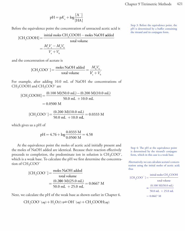
pH pAHAa= +−
K log[ ][ ]
Before the equivalence point the concentration of unreacted acetic acid is
[ ]CH COOHinitial moles CH COOH moles NaOH
33=
− aaddedtotal volume
a a b b
a b
=−+
M V M VV V
and the concentration of acetate is
[ ]CH COOmoles NaOH added
total volume3b b− = =
M VVV Va b+
For example, after adding 10.0 mL of NaOH the concentrations of CH3COOH and CH3COO– are
[ ]CH COOH(0.100 M)(50.0 mL) (0.200 M)(10.0
3 =− mL)
50.0 mL mLM
+=
10 00 0500
..
[ ]( .
.CH COO
M)(10.0 mL)50.0 mL m3
− =+
0 20010 0 LL
M= 0 0333.
which gives us a pH of
pHMM
= + =4 760 03330 0500
4 58. log..
.
At the equivalence point the moles of acetic acid initially present and the moles of NaOH added are identical. Because their reaction effectively proceeds to completion, the predominate ion in solution is CH3COO–, which is a weak base. To calculate the pH we first determine the concentra-tion of CH3COO–
[ ]
( .
CH COOmoles NaOH added
total volume3− =
=0 2000
25 00 0667
M)(25.0 mL)50.0 mL mL
M+
=.
.
Next, we calculate the pH of the weak base as shown earlier in Chapter 6.
CH COO H O OH CH COOH3 2 3− −+ +( ) ( ) ( ) ( )aq l aq aq
Alternatively, we can calculate acetate’s concen-tration using the initial moles of acetic acid; thus
[ ]CH COOinitial moles CH COOH
total volume33− =
==+
=
( .
.
.
0 100
25 0
0 0667
M)(50.0 mL)
50.0 mL mL
M
Step 3: Before the equivalence point, the pH is determined by a buffer containing the titrand and its conjugate form.
Step 4: The pH at the equivalence point is determined by the titrand’s conjugate form, which in this case is a weak base.
422 Analytical Chemistry 2.0
Practice Exercise 9.2Construct a titration curve for the titration of 25.0 mL of 0.125 M NH3 with 0.0625 M HCl.
Click here to review your answer to this exercise.
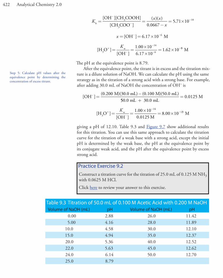
Kx x
xb3
3
OH CH COOHCH COO 0.0667
= =−
=−
−
[ ][ ][ ]
( )( )5..71 10 10� −
x = = �− −[ ] .OH M6 17 10 6
[ ][ ]
..
.H OOH3
w+−
−
−−= =
��
= �K 1 00 10
6 17 101 62 10
14
699 M
The pH at the equivalence point is 8.79.After the equivalence point, the titrant is in excess and the titration mix-
ture is a dilute solution of NaOH. We can calculate the pH using the same strategy as in the titration of a strong acid with a strong base. For example, after adding 30.0 mL of NaOH the concentration of OH– is
[ ]( . (
OHM)(30.0 mL) 0.100 M)(50.0 mL)− =
−0 200550.0 mL 30.0 mL
M+
= 0 0125.
[ ][ ]
..
.H OOH M3
w+−
−−= =
�= �
K 1 00 100 0125
8 00 1014
133 M
giving a pH of 12.10. Table 9.3 and Figure 9.7 show additional results for this titration. You can use this same approach to calculate the titration curve for the titration of a weak base with a strong acid, except the initial pH is determined by the weak base, the pH at the equivalence point by its conjugate weak acid, and the pH after the equivalence point by excess strong acid.
Table 9.3 Titration of 50.0 mL of 0.100 M Acetic Acid with 0.200 M NaOHVolume of NaOH (mL) pH Volume of NaOH (mL) pH
0.00 2.88 26.0 11.425.00 4.16 28.0 11.89
10.0 4.58 30.0 12.1015.0 4.94 35.0 12.3720.0 5.36 40.0 12.5222.0 5.63 45.0 12.6224.0 6.14 50.0 12.7025.0 8.79
Step 5: Calculate pH values after the equivalence point by determining the concentration of excess titrant.

423Chapter 9 Titrimetric Methods
We can extend our approach for calculating a weak acid–strong base titration curve to reactions involving multiprotic acids or bases, and mix-tures of acids or bases. As the complexity of the titration increases, however, the necessary calculations become more time consuming. Not surprisingly, a variety of algebraic1 and computer spreadsheet2 approaches have been described to aid in constructing titration curves.
SkeTching an acid–BaSe TiTraTion curve
To evaluate the relationship between a titration’s equivalence point and its end point, we need to construct only a reasonable approximation of the exact titration curve. In this section we demonstrate a simple method for sketching an acid–base titration curve. Our goal is to sketch the titration curve quickly, using as few calculations as possible. Let’s use the titration of 50.0 mL of 0.100 M CH3COOH with 0.200 M NaOH to illustrate our approach.
We begin by calculating the titration’s equivalence point volume, which, as we determined earlier, is 25.0 mL. Next we draw our axes, placing pH on the y-axis and the titrant’s volume on the x-axis. To indicate the equivalence point volume, we draw a vertical line corresponding to 25.0 mL of NaOH. Figure 9.8a shows the result of the first step in our sketch.
Before the equivalence point the titration mixture’s pH is determined by a buffer of acetic acid, CH3COOH, and acetate, CH3COO–. Although we can easily calculate a buffer’s pH using the Henderson–Hasselbalch equa-tion, we can avoid this calculation by making a simple assumption. You may recall from Chapter 6 that a buffer operates over a pH range extend-
1 (a) Willis, C. J. J. Chem. Educ. 1981, 58, 659–663; (b) Nakagawa, K. J. Chem. Educ. 1990, 67, 673–676; (c) Gordus, A. A. J. Chem. Educ. 1991, 68, 759–761; (d) de Levie, R. J. Chem. Educ. 1993, 70, 209–217; (e) Chaston, S. J. Chem. Educ. 1993, 70, 878–880; (f ) de Levie, R. Anal. Chem. 1996, 68, 585–590.
2 (a) Currie, J. O.; Whiteley, R. V. J. Chem. Educ. 1991, 68, 923–926; (b) Breneman, G. L.; Parker, O. J. J. Chem. Educ. 1992, 69, 46–47; (c) Carter, D. R.; Frye, M. S.; Mattson, W. A. J. Chem. Educ. 1993, 70, 67–71; (d) Freiser, H. Concepts and Calculations in Analytical Chemistry, CRC Press: Boca Raton, 1992.
Figure 9.7 Titration curve for the titration of 50.0 mL of 0.100 M CH3COOH with 0.200 M NaOH. The red points corre-spond to the data in Table 9.3. The blue line shows the complete titration curve.
This is the same example that we used in developing the calculations for a weak acid–strong base titration curve. You can review the results of that calculation in Table 9.3 and Figure 9.7.
0 10 20 30 40 50Volume of NaOH (mL)
0
2
4
6
8
10
12
14pH

424 Analytical Chemistry 2.0
Figure 9.8 Illustrations showing the steps in sketching an approximate titration curve for the titration of 50.0 mL of 0.100 M CH3COOH with 0.200 M NaOH: (a) locating the equivalence point volume; (b) plotting two points before the equivalence point; (c) plotting two points after the equivalence point; (d) preliminary approximation of titration curve using straight-lines; (e) final approximation of titration curve using a smooth curve; (f ) comparison of approximate titration curve (solid black line) and exact titration curve (dashed red line). See the text for additional details.
0 10 20 30 40 50Volume of NaOH (mL)
0
2
4
6
8
10
12
14
pH
(d)
0 10 20 30 40 50Volume of NaOH (mL)
0
2
4
6
8
10
12
14
pH
(a)
0 10 20 30 40 50Volume of NaOH (mL)
0
2
4
6
8
10
12
14
pH
(c)
0 10 20 30 40 50Volume of NaOH (mL)
0
2
4
6
8
10
12
14
pH
(f )(e)
0 10 20 30 40 50Volume of NaOH (mL)
0
2
4
6
8
10
12
14
pH
0 10 20 30 40 50Volume of NaOH (mL)
0
2
4
6
8
10
12
14
pH
(b)

425Chapter 9 Titrimetric Methods
ing approximately ±1 pH unit on either side of the weak acid’s pKa value. The pH is at the lower end of this range, pH = pKa – 1, when the weak acid’s concentration is 10� greater than that of its conjugate weak base. The buffer reaches its upper pH limit, pH = pKa + 1, when the weak acid’s concentration is 10� smaller than that of its conjugate weak base. When titrating a weak acid or a weak base, the buffer spans a range of volumes from approximately 10% of the equivalence point volume to approximately 90% of the equivalence point volume.
Figure 9.8b shows the second step in our sketch. First, we superimpose acetic acid’s ladder diagram on the y-axis, including its buffer range, using its pKa value of 4.76. Next, we add points representing the pH at 10% of the equivalence point volume (a pH of 3.76 at 2.5 mL) and at 90% of the equivalence point volume (a pH of 5.76 at 22.5 mL).
The third step in sketching our titration curve is to add two points after the equivalence point. The pH after the equivalence point is fixed by the concentration of excess titrant, NaOH. Calculating the pH of a strong base is straightforward, as we have seen earlier. Figure 9.8c shows the pH after adding 30.0 mL and 40.0 mL of NaOH.
Next, we draw a straight line through each pair of points, extending the lines through the vertical line representing the equivalence point’s volume (Figure 9.8d). Finally, we complete our sketch by drawing a smooth curve that connects the three straight-line segments (Figure 9.8e). A comparison of our sketch to the exact titration curve (Figure 9.8f ) shows that they are in close agreement.
The actual values are 9.09% and 90.9%, but for our purpose, using 10% and 90% is more convenient; that is, after all, one advantage of an approximation! Problem 9.4 in the end-of-chapter problems asks you to verify these percentages.
See Table 9.3 for the values.
Practice Exercise 9.3Sketch a titration curve for the titration of 25.0 mL of 0.125 M NH3 with 0.0625 M HCl and compare to the result from Practice Exercise 9.2.
Click here to review your answer to this exercise.As shown by the following example, we can adapt this approach to
acid–base titrations, including those involving polyprotic weak acids and bases, or mixtures of weak acids and bases.
Example 9.1
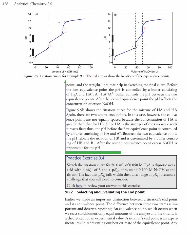
Sketch titration curves for the following two systems: (a) the titration of 50.0 mL of 0.050 M H2A, a diprotic weak acid with a pKa1 of 3 and a pKa2 of 7; and (b) the titration of a 50.0 mL mixture containing 0.075 M HA, a weak acid with a pKa of 3, and 0.025 M HB, a weak acid with a pKa of 7. For both titrations the titrant is 0.10 M NaOH.
Solution
Figure 9.9a shows the titration curve for H2A, including the ladder dia-gram on the y-axis, the equivalence points at 25.0 mL and 50.0 mL, two points before each equivalence point, two points after the last equivalence
426 Analytical Chemistry 2.0
point, and the straight-lines that help in sketching the final curve. Before the first equivalence point the pH is controlled by a buffer consisting of H2A and HA–. An HA–/A2– buffer controls the pH between the two equivalence points. After the second equivalence point the pH reflects the concentration of excess NaOH.Figure 9.9b shows the titration curve for the mixture of HA and HB. Again, there are two equivalence points. In this case, however, the equiva-lence points are not equally spaced because the concentration of HA is greater than that for HB. Since HA is the stronger of the two weak acids it reacts first; thus, the pH before the first equivalence point is controlled by a buffer consisting of HA and A–. Between the two equivalence points the pH reflects the titration of HB and is determined by a buffer consist-ing of HB and B–. After the second equivalence point excess NaOH is responsible for the pH.
Practice Exercise 9.4Sketch the titration curve for 50.0 mL of 0.050 M H2A, a diprotic weak acid with a pKa1 of 3 and a pKa2 of 4, using 0.100 M NaOH as the titrant. The fact that pKa2 falls within the buffer range of pKa1 presents a challenge that you will need to consider.
Click here to review your answer to this exercise.
Figure 9.9 Titration curves for Example 9.1. The red arrows show the locations of the equivalence points.
9B.2 Selecting and Evaluating the End point
Earlier we made an important distinction between a titration’s end point and its equivalence point. The difference between these two terms is im-portant and deserves repeating. An equivalence point, which occurs when we react stoichiometrically equal amounts of the analyte and the titrant, is a theoretical not an experimental value. A titration’s end point is an experi-mental result, representing our best estimate of the equivalence point. Any
0 20 40Volume of NaOH (mL)
0
2
4
6
8
10
12
14
pH
60 80 100 0 20 40Volume of NaOH (mL)
0
2
4
6
8
10
12
14
pH
60 80 100
(a) (b)

427Chapter 9 Titrimetric Methods
difference between an equivalence point and its corresponding end point is a source of determinate error. It is even possible that an equivalence point does not have a useful end point.
Where iS The equivalence PoinT?
Earlier we learned how to calculate the pH at the equivalence point for the titration of a strong acid with a strong base, and for the titration of a weak acid with a strong base. We also learned to quickly sketch a titration curve with only a minimum of calculations. Can we also locate the equivalence point without performing any calculations. The answer, as you might guess, is often yes!
For most acid–base titrations the inflection point, the point on a titra-tion curve having the greatest slope, very nearly coincides with the equiva-lence point.3 The red arrows in Figure 9.9, for example, indicate the equiva-lence points for the titration curves from Example 9.1. An inflection point actually precedes its corresponding equivalence point by a small amount, with the error approaching 0.1% for weak acids or weak bases with dissocia-tion constants smaller than 10–9, or for very dilute solutions.
The principal limitation to using an inflection point to locate the equiv-alence point is that the inflection point must be present. For some titrations the inflection point may be missing or difficult to find. Figure 9.10, for example, demonstrates the affect of a weak acid’s dissociation constant, Ka, on the shape of titration curve. An inflection point is visible, even if barely so, for acid dissociation constants larger than 10–9, but is missing when Ka is 10–11.
An inflection point also may be missing or difficult to detect if the analyte is a multiprotic weak acid or weak base with successive dissociation constants that are similar in magnitude. To appreciate why this is true let’s consider the titration of a diprotic weak acid, H2A, with NaOH. During the titration the following two reactions occur.
3 Meites, L.; Goldman, J. A. Anal. Chim. Acta 1963, 29, 472–479.
Figure 9.10 Weak acid–strong base titration curves for the titra-tion of 50.0 mL of 0.100 M HA with 0.100 M NaOH. The pKa values for HA are (a) 1, (b) 3, (c) 5, (d) 7, (e) 9, and (f ) 11.0 10 20 30 40 50 60 70
0
2
4
6
8
10
12
14
Volume of NaOH (mL)
pH
(a)(b)
(c)
(d)
(e)
(f )
428 Analytical Chemistry 2.0
H A OH HA H O2 2( ) ( ) ( ) ( )aq aq aq l+ → +− − 9.3
HA OH A H O2− − −+ → +( ) ( ) ( ) ( )aq aq aq l2 9.4
To see two distinct inflection points, reaction 9.3 must be essentially com-plete before reaction 9.4 begins.
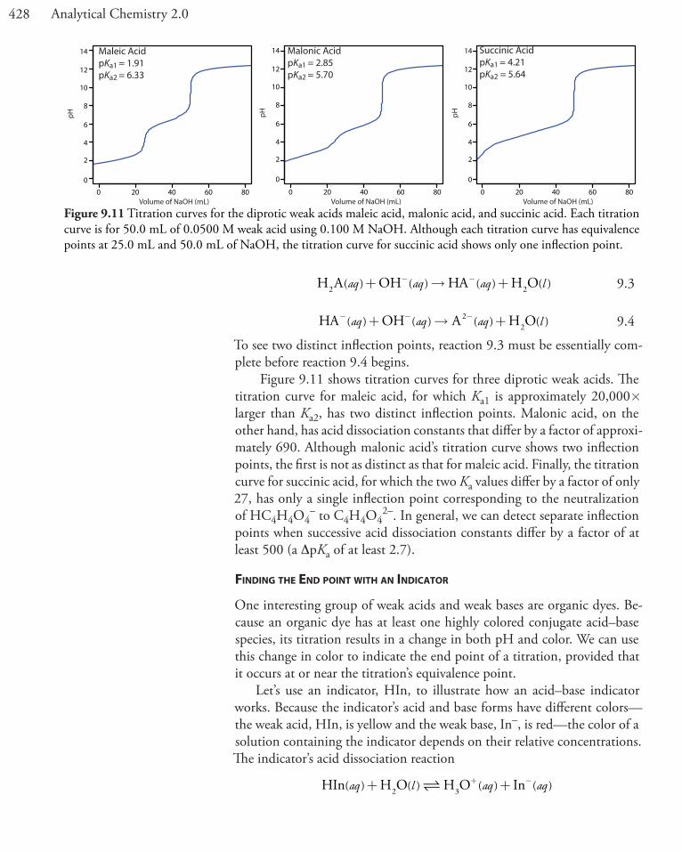
Figure 9.11 shows titration curves for three diprotic weak acids. The titration curve for maleic acid, for which Ka1 is approximately 20,000� larger than Ka2, has two distinct inflection points. Malonic acid, on the other hand, has acid dissociation constants that differ by a factor of approxi-mately 690. Although malonic acid’s titration curve shows two inflection points, the first is not as distinct as that for maleic acid. Finally, the titration curve for succinic acid, for which the two Ka values differ by a factor of only 27, has only a single inflection point corresponding to the neutralization of HC4H4O4
– to C4H4O42–. In general, we can detect separate inflection
points when successive acid dissociation constants differ by a factor of at least 500 (a DpKa of at least 2.7).
Finding The end PoinT WiTh an indicaTor
One interesting group of weak acids and weak bases are organic dyes. Be-cause an organic dye has at least one highly colored conjugate acid–base species, its titration results in a change in both pH and color. We can use this change in color to indicate the end point of a titration, provided that it occurs at or near the titration’s equivalence point.
Let’s use an indicator, HIn, to illustrate how an acid–base indicator works. Because the indicator’s acid and base forms have different colors—the weak acid, HIn, is yellow and the weak base, In–, is red—the color of a solution containing the indicator depends on their relative concentrations. The indicator’s acid dissociation reaction
HIn H O H O In2 3( ) ( ) ( ) ( )aq l aq aq+ ++ −
Figure 9.11 Titration curves for the diprotic weak acids maleic acid, malonic acid, and succinic acid. Each titration curve is for 50.0 mL of 0.0500 M weak acid using 0.100 M NaOH. Although each titration curve has equivalence points at 25.0 mL and 50.0 mL of NaOH, the titration curve for succinic acid shows only one inflection point.
0
2
4
6
8
10
12
14
pH
0 20 40 60 80Volume of NaOH (mL)
Maleic AcidpKa1 = 1.91pKa2 = 6.33
0
2
4
6
8
10
12
14
pH
0 20 40 60 80Volume of NaOH (mL)
Malonic AcidpKa1 = 2.85pKa2 = 5.70
0 20 40 60 80
0
2
4
6
8
10
12
14
Volume of NaOH (mL)
pH
Succinic AcidpKa1 = 4.21pKa2 = 5.64

429Chapter 9 Titrimetric Methods
has an equilibrium constant of
K a3H O In
HIn=
+ −[ ][ ][ ]
9.5
Taking the negative log of each side of equation 9.5, and rearranging to solve for pH leaves with a equation
pH pInHIna= +
−
K log[ ][ ]
9.6
relating the solution’s pH to the relative concentrations of HIn and In–. If we can detect HIn and In– with equal ease, then the transition from
yellow to red (or from red to yellow) reaches its midpoint, which is orange, when their concentrations are equal, or when the pH is equal to the indi-cator’s pKa. If the indicator’s pKa and the pH at the equivalence point are identical, then titrating until the indicator turns orange is a suitable end point. Unfortunately, we rarely know the exact pH at the equivalence point. In addition, determining when the concentrations of HIn and In– are equal may be difficult if the indicator’s change in color is subtle.
We can establish the range of pHs over which the average analyst observes a change in the indicator’s color by making the following assumptions—the indicator’s color is yellow if the concentration of HIn is 10� greater than that of In–, and its color is red if the concentration of HIn is 10� smaller than that of In–. Substituting these inequalities into equation 9.6
pH p pa a= + = −K Klog1
101
pH p pa a= + = +K Klog101
1
shows that the indicator changes color over a pH range extending ±1 unit on either side of its pKa. As shown in Figure 9.12, the indicator is yellow when the pH is less than pKa – 1, and it is red for pHs greater than pKa + 1.
Figure 9.12 Diagram showing the relationship between pH and an indicator’s color. The ladder diagram defines pH val-ues where HIn and In– are the predominate species. The indicator changes color when the pH is between pKa – 1 and pKa + 1.
In–
HIn
pH = pKa,HIn
indicator’scolor transition
range
indicatoris color of In–
indicatoris color of HIn
pH

430 Analytical Chemistry 2.0
For pHs between pKa – 1 and pKa + 1 the indicator’s color passes through various shades of orange. The properties of several common acid–base in-dicators are shown in Table 9.4.
The relatively broad range of pHs over which an indicator changes color places additional limitations on its feasibility for signaling a titration’s end point. To minimize a determinate titration error, an indicator’s entire pH range must fall within the rapid change in pH at the equivalence point. For example, in Figure 9.13 we see that phenolphthalein is an appropriate indicator for the titration of 50.0 mL of 0.050 M acetic acid with 0.10 M NaOH. Bromothymol blue, on the other hand, is an inappropriate indica-tor because its change in color begins before the initial sharp rise in pH, and, as a result, spans a relatively large range of volumes. The early change in color increases the probability of obtaining inaccurate results, while the range of possible end point volumes increases the probability of obtaining imprecise results.
Practice Exercise 9.5Suggest a suitable indicator for the titration of 25.0 mL of 0.125 M NH3 with 0.0625 M NaOH. You constructed a titration curve for this titra-tion in Practice Exercise 9.2 and Practice Exercise 9.3.
Click here to review your answer to this exercise.
You may wonder why an indicator’s pH range, such as that for phenolphthalein, is not equally distributed around its pKa val-ue. The explanation is simple. Figure 9.12 presents an idealized view of an indicator in which our sensitivity to the indicator’s two colors is equal. For some indicators only the weak acid or the weak base is col-ored. For other indicators both the weak acid and the weak base are colored, but one form is easier to see. In either case, the indicator’s pH range is skewed in the direction of the indicator’s less colored form. Thus, phenolphthalein’s pH range is skewed in the direction of its colorless form, shifting the pH range to values low-er than those suggested by Figure 9.12.
Table 9.4 Properties of Selected Acid–Base Indicators
IndicatorAcid Color
Base Color pH Range pKa
cresol red red yellow 0.2–1.8 –thymol blue red yellow 1.2–2.8 1.7bromophenol blue yellow blue 3.0–4.6 4.1methyl orange red yellow 3.1–4.4 3.7Congo red blue red 3.0–5.0 –bromocresol green yellow blue 3.8–5.4 4.7methyl red red yellow 4.2–6.3 5.0bromocresol purple yellow purple 5.2–6.8 6.1litmus red blue 5.0–8.0 –bromothymol blue yellow blue 6.0–7.6 7.1phenol red yellow blue 6.8–8.4 7.8cresol red yellow red 7.2–8.8 8.2thymol blue yellow red 8.0–9.6 8.9phenolphthalein colorless red 8.3–10.0 9.6alizarin yellow R yellow orange–red 10.1–12.0 –

431Chapter 9 Titrimetric Methods
Finding The end PoinT By MoniToring Ph
An alternative approach for locating a titration’s end point is to continu-ously monitor the titration’s progress using a sensor whose signal is a func-tion of the analyte’s concentration. The result is a plot of the entire titration curve, which we can use to locate the end point with a minimal error.
The obvious sensor for monitoring an acid–base titration is a pH elec-trode and the result is a potentiometric titration curve. For example, Figure 9.14a shows a small portion of the potentiometric titration curve for the titration of 50.0 mL of 0.050 M CH3COOH with 0.10 M NaOH, fo-cusing on the region containing the equivalence point. The simplest meth-od for finding the end point is to locate the titration curve’s inflection point, as shown by the arrow. This is also the least accurate method, particularly if the titration curve has a shallow slope at the equivalence point.
Another method for locating the end point is to plot the titration curve’s first derivative, which gives the titration curve’s slope at each point along the x-axis. Examine Figure 9.14a and consider how the titration curve’s slope changes as we approach, reach, and pass the equivalence point. Be-cause the slope reaches its maximum value at the inflection point, the first derivative shows a spike at the equivalence point (Figure 9.14b).
The second derivative of a titration curve may be more useful than the first derivative because the equivalence point intersects the volume axis. Figure 9.14c shows the resulting titration curve.
Derivative methods are particularly useful when titrating a sample that contains more than one analyte. If we rely on indicators to locate the end points, then we usually must complete separate titrations for each analyte. If we record the titration curve, however, then a single titration is sufficient.
Figure 9.13 Portion of the titration curve for 50.0 mL of 0.050 M CH3COOH with 0.10 M NaOH, highlighting the region containing the equivalence point. The end point transitions for the indicators phenolphthalein and bromothymol blue are superimposed on the titration curve.
See Chapter 11 for more details about pH electrodes.
23 24 25 26 27Volume of NaOH (mL)
7
9
6
8
10
12
11
pH
phenolphthalein’s pH range
bromothymol blue’spH range

432 Analytical Chemistry 2.0
The precision with which we can locate the end point also makes derivative methods attractive for an analyte with a poorly defined normal titration curve.
Derivative methods work well only if we record sufficient data during the rapid increase in pH near the equivalence point. This is usually not a problem if we use an automatic titrator, such as that seen earlier in Fig-ure 9.5. Because the pH changes so rapidly near the equivalence point—a change of several pH units with the addition of several drops of titrant is not unusual—a manual titration does not provide enough data for a useful derivative titration curve. A manual titration does contain an abundance of data during the more gently rising portions of the titration curve before and after the equivalence point. This data also contains information about the titration curve’s equivalence point.
Consider again the titration of acetic acid, CH3COOH, with NaOH. At any point during the titration acetic acid is in equilibrium with H3O+ and CH3COO–
CH COOH H O H O CH COO3 2 3 3( ) ( ) ( ) ( )aq l aq aq+ ++ −
for which the equilibrium constant is
K a3 3
3
H O CH COOCH COOH
=+ −[ ][ ]
[ ]
Figure 9.14 Titration curves for the titra-tion of 50.0 mL of 0.050 M CH3COOH with 0.10 M NaOH: (a) normal titration curve; (b) first derivative titration curve; (c) second derivative titration curve; (d) Gran plot. The red arrow shows the loca-tion of the titration’s end point.
Suppose we have the following three points on our titration curve:
volume (mL) pH
23.65 6.00
23.91 6.10
24.13 6.20
Mathematically, we can approximate the first derivative as DpH/DV, where DpH is the change in pH between successive addi-tions of titrant. Using the first two points, the first derivative is
∆pH
∆V=
−
−=
6 10 6 00
23 91 23 650 385
. .
. ..
which we assign to the average of the two volumes, or 23.78 mL. For the second and third points, the first derivative is 0.455 and the average volume is 24.02 mL.
volume (mL) DpH/DV
23.78 0.385
24.02 0.455
We can approximate the second derivative as D(DpH/DV)/DV, or D2pH/DV 2. Using the two points from our calculation of the first derivative, the second derivative is
∆ pH
∆
2
2
0 455 0 385
23 78 24 020 292
V=
−
−=
. .
. ..
Note that calculating the first derivative comes at the expense of losing one piece of information (three points become two points), and calculating the second deriv-ative comes at the expense of losing two pieces of information.
23 24 25 26 27
5
6
7
8
9
10
11
12
Volume of NaOH (mL)
pH
0
10
20
30
40
50
60
23 24 25 26 27Volume of NaOH (mL)
ΔpH
/ΔV
-2000
0
2000
4000
23 24 25 26 27Volume of NaOH (mL)
Δ2 pH
/ΔV2
0e+00
1e-05
2e-05
3e-05
4e-05
5e-05
23 24 25 26 27Volume of NaOH (mL)
V b×[
H3O
+ ]
(a) (b)
(c) (d)
433Chapter 9 Titrimetric Methods
Before the equivalence point the concentrations of CH3COOH and CH3COO– are
[ ]CH COOHinitial moles CH COOH moles NaOH
33=
− aaddedtotal volume
a a b b
a b
=−+
M V M VV V
[ ]CH COOmoles NaOH added
total volume3b b− = =
M VVV Va b+
Substituting these equations into the Ka expression and rearranging leaves us with
KM V
M V M Va3 b b
a a b b
H O=
−
+[ ]( )
K M V K M V M Va a a a b b 3 b bH O− = +[ ]( )
K M VM
K V Va a a
ba b 3 bH O− = �+[ ]
Finally, recognizing that the equivalence point volume is
VM VMeq
a a
b
=
leaves us with the following equation.
[ ]H O3 b a eq a b+ � = −V K V K V
For volumes of titrant before the equivalence point, a plot of Vb�[H3O+] versus Vb is a straight-line with an x-intercept of Veq and a slope of –Ka. Figure 9.14d shows a typical result. This method of data analysis, which converts a portion of a titration curve into a straight-line, is a Gran plot.
Finding The end PoinT By MoniToring TeMPeraTure
The reaction between an acid and a base is exothermic. Heat generated by the reaction is absorbed by the titrand, increasing its temperature. Monitor-ing the titrand’s temperature as we add the titrant provides us with another method for recording a titration curve and identifying the titration’s end point (Figure 9.15).
Before adding titrant, any change in the titrand’s temperature is the re-sult of warming or cooling as it equilibrates with the surroundings. Adding titrant initiates the exothermic acid–base reaction, increasing the titrand’s temperature. This part of a thermometric titration curve is called the titra-

434 Analytical Chemistry 2.0
tion branch. The temperature continues to rise with each addition of titrant until we reach the equivalence point. After the equivalence point, any change in temperature is due to the titrant’s enthalpy of dilution, and the difference between the temperatures of the titrant and titrand. Ideally, the equivalence point is a distinct intersection of the titration branch and the excess titrant branch. As shown in Figure 9.15, however, a thermometric titration curve usually shows curvature near the equivalence point due to an incomplete neutralization reaction, or to the excessive dilution of the titrand and the titrant during the titration. The latter problem is minimized by using a titrant that is 10–100 times more concentrated than the analyte, although this results in a very small end point volume and a larger relative error. If necessary, the end point is found by extrapolation.
Although not a particularly common method for monitoring acid–base titrations, a thermometric titration has one distinct advantage over the direct or indirect monitoring of pH. As discussed earlier, the use of an indicator or the monitoring of pH is limited by the magnitude of the rele-vant equilibrium constants. For example, titrating boric acid, H3BO3, with NaOH does not provide a sharp end point when monitoring pH because, boric acid’s Ka of 5.8 � 10–10 is too small (Figure 9.16a). Because boric acid’s enthalpy of neutralization is fairly large, –42.7 kJ/mole, however, its thermometric titration curve provides a useful endpoint (Figure 9.16b).
9B.3 Titrations in Nonaqueous Solvents
Thus far we have assumed that the titrant and the titrand are aqueous solu-tions. Although water is the most common solvent in acid–base titrimetry, switching to a nonaqueous solvent can improve a titration’s feasibility.
For an amphoteric solvent, SH, the autoprotolysis constant, Ks, relates the concentration of its protonated form, SH2
+, to that of its deprotonated form, S–
Figure 9.15 Typical thermometric titration curve. The endpoint, shown by the red arrow, is found by extrapolating the titration branch and the excess titration branch. Volume of Titrant
Tem
pera
ture
0
Titr
atio
n Br
anch
Excess Titrant Branch

435Chapter 9 Titrimetric Methods
2 2SH SH S
+ −+
K s SH S= + −[ ][ ]2
and the solvent’s pH and pOH are
pH SH=− +log[ ]2
pOH S=− −log[ ]
The most important limitation imposed by Ks is the change in pH dur-ing a titration. To understand why this is true, let’s consider the titration of 50.0 mL of 1.0�10–4 M HCl using 1.0�10–4 M NaOH. Before the equivalence point, the pH is determined by the untitrated strong acid. For example, when the volume of NaOH is 90% of Veq, the concentration of H3O+ is
[ ]
( .
H O
M)(50.0 mL)
3a a b b
a b
+
−
=−+
=�
M V M VV V
1 0 10 4 −− �+
=
−( ..
.
1 0 1045 0
5 3
4 M)(45.0 mL)50.0 mL mL
�� −10 6 M
and the pH is 5.3. When the volume of NaOH is 110% of Veq, the con-centration of OH– is
[ ]
( .
OH
M)(55.0 mL)
b b a a
a b
−
−
=−+
=� −
M V M VV V
1 0 10 4 (( ..
.
1 0 1055 0
4 8
4�+
= �
− M)(50.0 mL)50.0 mL mL
110 6− M
Figure 9.16 Titration curves for the titration of 50.0 mL of 0.050 M H3BO3 with 0.50 M NaOH obtained by monitoring (a) pH, and (b) temperature. The red arrows show the end points for the titrations.
You should recognize that Kw is just spe-cific form of Ks when the solvent is wa-ter.
The titration’s equivalence point requires 50.0 mL of NaOH; thus, 90% of Veq is 45.0 mL of NaOH.
The titration’s equivalence point requires 50.0 mL of NaOH; thus, 110% of Veq is 55.0 mL of NaOH.
0
2
4
6
8
10
12
14
0 2 4 6 8 10Volume of NaOH (mL)
pH
0 2 4 6 8 10
25.0
25.1
25.2
25.3
25.4
25.5
25.6
Volume of NaOH (mL)
Tem
pera
ture
(o C)
(a) (b)

436 Analytical Chemistry 2.0
and the pOH is 5.3. The titrand’s pH is
pH p pOHw= − = − =K 14 5 3 8 7. .
and the change in the titrand’s pH as the titration goes from 90% to 110% of Veq is
∆pH= − =8 7 5 3 3 4. . .
If we carry out the same titration in a nonaqueous solvent with a Ks of 1.0�10–20, the pH after adding 45.0 mL of NaOH is still 5.3. However, the pH after adding 55.0 mL of NaOH is
pH p pOHs= − = − =K 20 5 3 14 7. .
In this case the change in pH ∆pH= − =14 7 5 3 9 4. . .
is significantly greater than that obtained when the titration is carried out in water. Figure 9.17 shows the titration curves in both the aqueous and the nonaqueous solvents.
Another parameter affecting the feasibility of an acid–base titration is the titrand’s dissociation constant. Here, too, the solvent plays an impor-tant role. The strength of an acid or a base is a relative measure of the ease transferring a proton from the acid to the solvent, or from the solvent to the base. For example, HF, with a Ka of 6.8 � 10–4, is a better proton donor than CH3COOH, for which Ka is 1.75 � 10–5.
The strongest acid that can exist in water is the hydronium ion, H3O+. HCl and HNO3 are strong acids because they are better proton donors than H3O+ and essentially donate all their protons to H2O, levelinG their acid
Figure 9.17 Titration curves for 50.0 mL of 1.0 � 10–4 M HCl using 1.0 � 10–4 M NaOH in (a) water, Kw = 1.0 � 10–14, and (b) a nonaqueous solvent, Ks = 1.0 � 10–20.
0 20 40 60 80 100
0
5
10
15
20
pH
Volume of NaOH(mL)
(b)
(a)

437Chapter 9 Titrimetric Methods
Representative Method 9.1Determination of Protein in Bread
Description of the MethoD
This method is based on a determination of %w/w nitrogen using the Kjeldahl method. The protein in a sample of bread is oxidized to NH4
+ using hot concentrated H2SO4. After making the solution alkaline, which converts the NH4
+ to NH3, the ammonia is distilled into a flask con-taining a known amount of HCl. The amount of unreacted HCl is de-termined by a back titration with standard strong base titrant. Because different cereal proteins contain similar amounts of nitrogen, multiplying the experimentally determined %w/w N by a factor of 5.7 gives the %w/w protein in the sample (on average there are 5.7 g protein for every gram of nitrogen).
proceDure
Transfer a 2.0-g sample of bread, which has previously been air-dried and ground into a powder, to a suitable digestion flask, along with 0.7 g of a HgO catalyst, 10 g of K2SO4, and 25 mL of concentrated H2SO4. Bring the solution to a boil. Continue boiling until the solution turns clear and then boil for at least an additional 30 minutes. After cooling the solution
The best way to appreciate the theoretical and practical details discussed in this sec-tion is to carefully examine a typical acid–base titrimetric method. Although each method is unique, the following descrip-tion of the determination of protein in bread provides an instructive example of a typical procedure. The description here is based on Method 13.86 as published in Official Methods of Analysis, 8th Ed., Asso-ciation of Official Agricultural Chemists: Washington, D. C., 1955.
strength to that of H3O+. In a different solvent HCl and HNO3 may not behave as strong acids.
If we place acetic acid in water the dissociation reaction
CH COOH H O H O CH COO3 2 3 3( ) ( ) ( ) ( )aq l aq aq+ ++ −
does not proceed to a significant extent because CH3COO– is a stronger base than H2O, and H3O+ is a stronger acid than CH3COOH. If we place acetic acid in a solvent, such as ammonia, that is a stronger base than water, then the reaction
CH COOH NH NH CH COO3 3+ ++ −3 4
proceeds to a greater extent. In fact, both HCl and CH3COOH are strong acids in ammonia.
All other things being equal, the strength of a weak acid increases if we place it in a solvent that is more basic than water, and the strength of a weak base increases if we place it in a solvent that is more acidic than water. In some cases, however, the opposite effect is observed. For example, the pKb for NH3 is 4.75 in water and it is 6.40 in the more acidic glacial acetic acid. In contradiction to our expectations, NH3 is a weaker base in the more acidic solvent. A full description of the solvent’s effect on the pKa of weak acid or the pKb of a weak base is beyond the scope of this text. You should be aware, however, that a titration that is not feasible in water may be feasible in a different solvent.
438 Analytical Chemistry 2.0
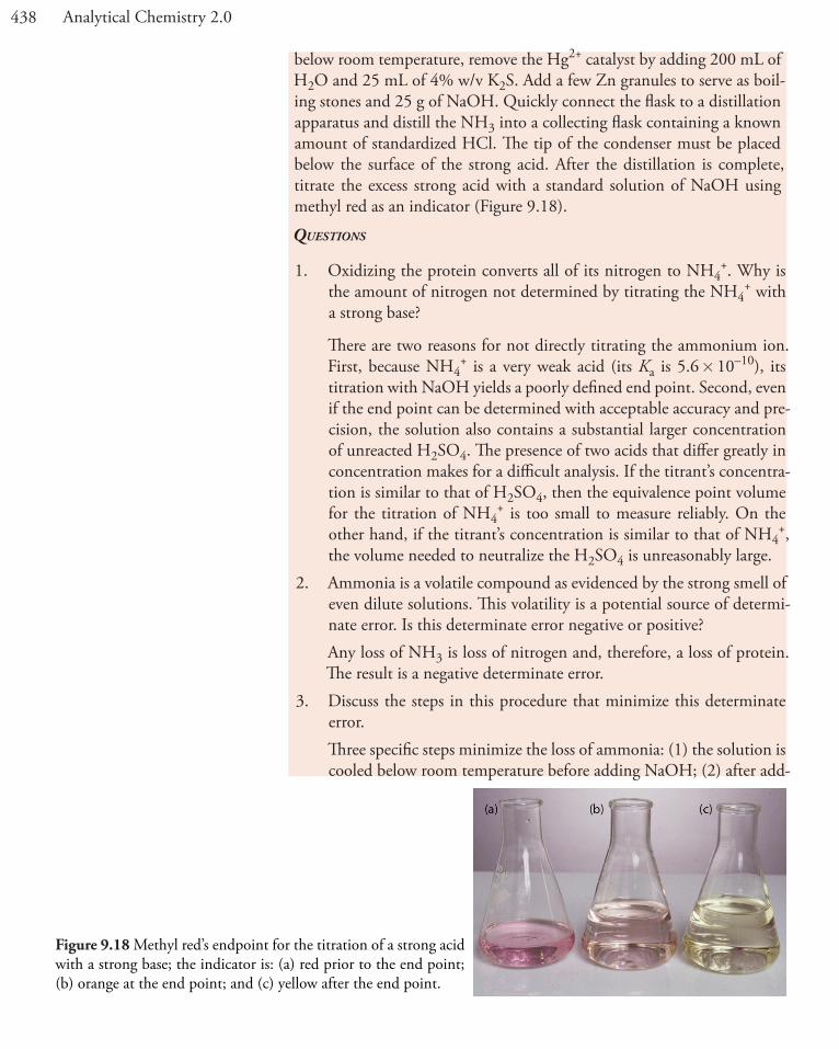
below room temperature, remove the Hg2+ catalyst by adding 200 mL of H2O and 25 mL of 4% w/v K2S. Add a few Zn granules to serve as boil-ing stones and 25 g of NaOH. Quickly connect the flask to a distillation apparatus and distill the NH3 into a collecting flask containing a known amount of standardized HCl. The tip of the condenser must be placed below the surface of the strong acid. After the distillation is complete, titrate the excess strong acid with a standard solution of NaOH using methyl red as an indicator (Figure 9.18).
Questions
1. Oxidizing the protein converts all of its nitrogen to NH4+. Why is
the amount of nitrogen not determined by titrating the NH4+ with
a strong base?
There are two reasons for not directly titrating the ammonium ion. First, because NH4
+ is a very weak acid (its Ka is 5.6 � 10–10), its titration with NaOH yields a poorly defined end point. Second, even if the end point can be determined with acceptable accuracy and pre-cision, the solution also contains a substantial larger concentration of unreacted H2SO4. The presence of two acids that differ greatly in concentration makes for a difficult analysis. If the titrant’s concentra-tion is similar to that of H2SO4, then the equivalence point volume for the titration of NH4
+ is too small to measure reliably. On the other hand, if the titrant’s concentration is similar to that of NH4
+, the volume needed to neutralize the H2SO4 is unreasonably large.
2. Ammonia is a volatile compound as evidenced by the strong smell of even dilute solutions. This volatility is a potential source of determi-nate error. Is this determinate error negative or positive?
Any loss of NH3 is loss of nitrogen and, therefore, a loss of protein. The result is a negative determinate error.
3. Discuss the steps in this procedure that minimize this determinate error.
Three specific steps minimize the loss of ammonia: (1) the solution is cooled below room temperature before adding NaOH; (2) after add-
Figure 9.18 Methyl red’s endpoint for the titration of a strong acid with a strong base; the indicator is: (a) red prior to the end point; (b) orange at the end point; and (c) yellow after the end point.

439Chapter 9 Titrimetric Methods
9B.4 quanTiTaTive aPPlicaTionS
Although many quantitative applications of acid–base titrimetry have been replaced by other analytical methods, a few important applications con-tinue to be relevant. In this section we review the general application of acid–base titrimetry to the analysis of inorganic and organic compounds, with an emphasis on applications in environmental and clinical analysis. First, however, we discuss the selection and standardization of acidic and basic titrants.
SelecTing and STandardizing a TiTranT
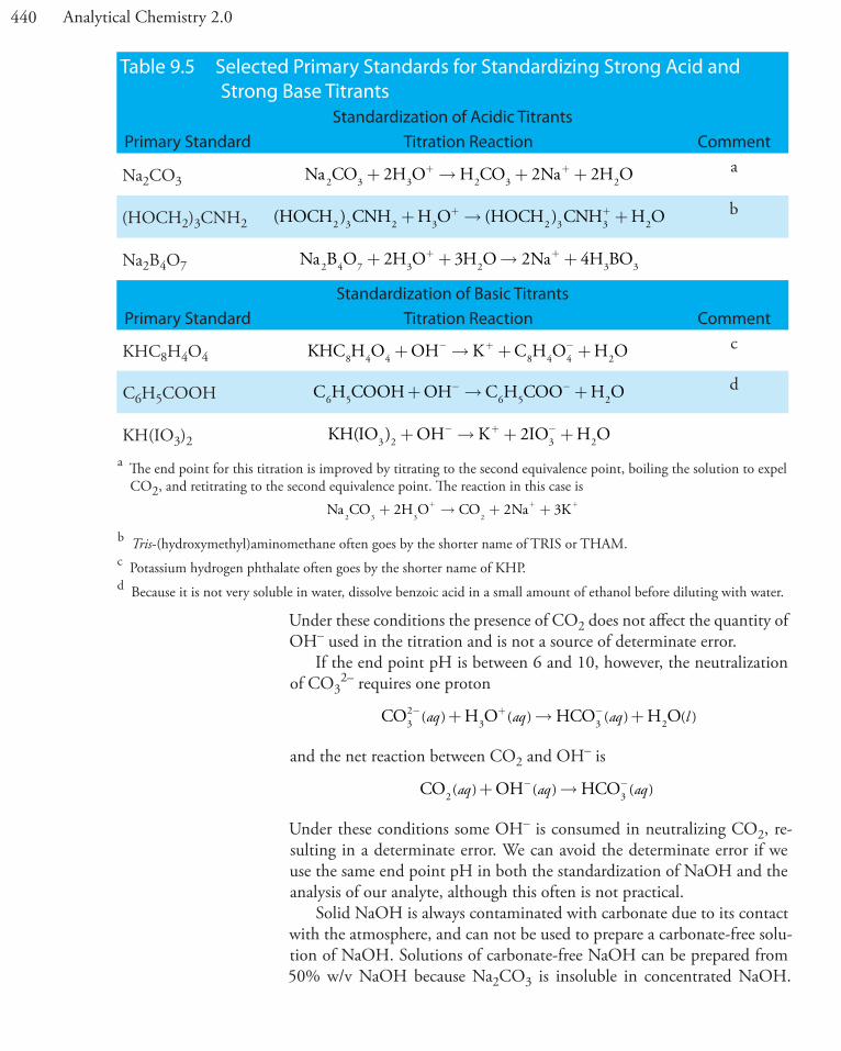
The most common strong acid titrants are HCl, HClO4, and H2SO4. So-lutions of these titrants are usually prepared by diluting a commercially available concentrated stock solution. Because the concentrations of con-centrated acids are known only approximately, the titrant’s concentration is determined by standardizing against one of the primary standard weak bases listed in Table 9.5.
The most common strong base titrant is NaOH. Sodium hydroxide is available both as an impure solid and as an approximately 50% w/v solu-tion. Solutions of NaOH may be standardized against any of the primary weak acid standards listed in Table 9.5.
Using NaOH as a titrant is complicated by potential contamination from the following reaction between CO2 and OH–.
CO OH CO H O22 322( ) ( ) ( ) ( )aq aq aq l+ → +− − 9.7
During the titration, NaOH reacts with both the titrand and CO2, increas-ing the volume of NaOH needed to reach the titration’s end point. This is not a problem if end point pH is less than 6. Below this pH the CO3
2– from reaction 9.7 reacts with H3O+ to form carbonic acid.
CO H O H CO H O3 2 3 232 2 2− ++ → +( ) ( ) ( ) ( )aq aq aq l 9.8
Combining reaction 9.7 and reaction 9.8 gives an overall reaction that does not include OH–.
CO H O H CO2 22 3( ) ( ) ( )aq l aq+ →
The nominal concentrations of the con-centrated stock solutions are 12.1 M HCl, 11.7 M HClO4, and 18.0 M H2SO4.
Any solution in contact with the at-mosphere contains a small amount of CO2(aq) from the equilibrium
CO CO2 2( ) ( )g aq
ing NaOH, the digestion flask is quickly connected to the distillation apparatus; and (3) the condenser’s tip is placed below the surface of the HCl to ensure that the NH3 reacts with the HCl before it can be lost through volatilization.
4. How does K2S remove Hg2+, and why is its removal important? Adding sulfide precipitates Hg2+ as HgS. This is important because
NH3 forms stable complexes with many metal ions, including Hg2+. Any NH3 that reacts with Hg2+ is not collected during distillation, providing another source of determinate error.
440 Analytical Chemistry 2.0
Under these conditions the presence of CO2 does not affect the quantity of OH– used in the titration and is not a source of determinate error.
If the end point pH is between 6 and 10, however, the neutralization of CO3
2– requires one proton
CO H O HCO H O3 232
3− + −+ → +( ) ( ) ( ) ( )aq aq aq l
and the net reaction between CO2 and OH– is
CO OH HCO32( ) ( ) ( )aq aq aq+ →− −
Under these conditions some OH– is consumed in neutralizing CO2, re-sulting in a determinate error. We can avoid the determinate error if we use the same end point pH in both the standardization of NaOH and the analysis of our analyte, although this often is not practical.
Solid NaOH is always contaminated with carbonate due to its contact with the atmosphere, and can not be used to prepare a carbonate-free solu-tion of NaOH. Solutions of carbonate-free NaOH can be prepared from 50% w/v NaOH because Na2CO3 is insoluble in concentrated NaOH.
Table 9.5 Selected Primary Standards for Standardizing Strong Acid and Strong Base Titrants
Standardization of Acidic TitrantsPrimary Standard Titration Reaction Comment
Na2CO3 Na CO H O H CO Na H O2 3 2 23 32 2 2+ → + ++ + a
(HOCH2)3CNH2 ( ) ( )HOCH CNH H O HOCH CNH H O3 22 3 2 2 3 3+ → ++ + b
Na2B4O7 Na B O H O H O Na H BO2 4 7 3 2 3 3+ + → ++ +2 3 2 4
Standardization of Basic TitrantsPrimary Standard Titration Reaction Comment
KHC8H4O4 KHC H O OH K C H O H O8 4 4 8 4 4 2+ → + +− + − c
C6H5COOH C H COOH OH C H COO H O6 5 6 5 2+ → +− − d
KH(IO3)2 KH(IO OH K IO H O3 3 2)2 2+ → + +− + −
a The end point for this titration is improved by titrating to the second equivalence point, boiling the solution to expel CO2, and retitrating to the second equivalence point. The reaction in this case is
Na CO H O CO Na K2 3 3 2
+ → + ++ + +2 2 3
b Tris-(hydroxymethyl)aminomethane often goes by the shorter name of TRIS or THAM.c Potassium hydrogen phthalate often goes by the shorter name of KHP.d Because it is not very soluble in water, dissolve benzoic acid in a small amount of ethanol before diluting with water.
441Chapter 9 Titrimetric Methods
When CO2 is absorbed, Na2CO3 precipitates and settles to the bottom of the container, allowing access to the carbonate-free NaOH. When prepar-ing a solution of NaOH, be sure to use water that is free from dissolved CO2. Briefly boiling the water expels CO2, and after cooling, it may be used to prepare carbonate-free solutions of NaOH. A solution of carbonate-free NaOH is relatively stable f we limit its contact with the atmosphere. Stan-dard solutions of sodium hydroxide should not be stored in glass bottles as NaOH reacts with glass to form silicate; instead, store such solutions in polyethylene bottles.
inorganic analySiS
Acid –base titrimetry is a standard method for the quantitative analysis of many inorganic acids and bases. A standard solution of NaOH can be used to determine the concentration of inorganic acids, such as H3PO4 or H3AsO4, and inorganic bases, such as Na2CO3 can be analyzed using a standard solution of HCl.
An inorganic acid or base that is too weak to be analyzed by an aqueous acid–base titration can be analyzed by adjusting the solvent, or by an in-direct analysis. For example, when analyzing boric acid, H3BO3, by titrat-ing with NaOH, accuracy is limited by boric acid’s small acid dissociation constant of 5.8 � 10–10. Boric acid’s Ka value increases to 1.5 � 10–4 in the presence of mannitol, because it forms a complex with the borate ion. The result is a sharper end point and a more accurate titration. Similarly, the analysis of ammonium salts is limited by the small acid dissociation con-stant of 5.7 � 10–10 for NH4
+. In this case, we can convert NH4+ to NH3
by neutralizing with strong base. The NH3, for which Kb is 1.58� 10–5, is then removed by distillation and titrated with HCl.
We can analyze a neutral inorganic analyte if we can first convert it into an acid or base. For example, we can determine the concentration of NO3
– by reducing it to NH3 in a strongly alkaline solution using Devarda’s alloy, a mixture of 50% w/w Cu, 45% w/w Al, and 5% w/w Zn.
3 8 5 2 83 2NO Al OH H O AlO2− − −+ + + →( ) ( ) ( ) ( ) (aq s aq l aq )) ( )+ 3 3NH aq
The NH3 is removed by distillation and titrated with HCl. Alternatively, we can titrate NO3
– as a weak base by placing it in an acidic nonaqueous solvent such as anhydrous acetic acid and using HClO4 as a titrant.
Acid–base titrimetry continues to be listed as a standard method for the determination of alkalinity, acidity, and free CO2 in waters and wastewaters. Alkalinity is a measure of a sample’s capacity to neutralize acids. The most important sources of alkalinity are OH–, HCO3
–, and CO32–, although
other weak bases, such as phosphate, may contribute to the overall alkalin-ity. Total alkalinity is determined by titrating to a fixed end point pH of 4.5 (or to the bromocresol green end point) using a standard solution of HCl or H2SO4. Results are reported as mg CaCO3/L.
Although a variety of strong bases and weak bases may contribute to a sample’s alkalinity, a single titration cannot distin-guish between the possible sources. Re-porting the total alkalinity as if CaCO3 is the only source provides a means for com-paring the acid-neutralizing capacities of different samples.
Figure 9.16a shows a typical result for the titration of H3BO3 with NaOH.
442 Analytical Chemistry 2.0
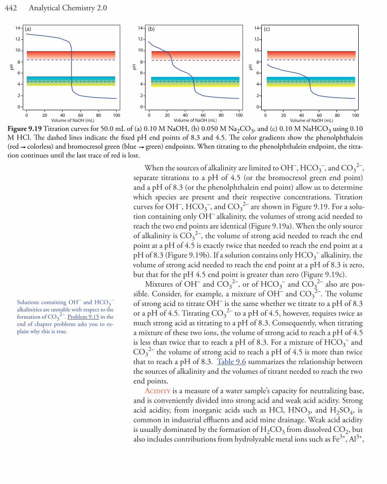
When the sources of alkalinity are limited to OH–, HCO3–, and CO3
2–, separate titrations to a pH of 4.5 (or the bromocresol green end point) and a pH of 8.3 (or the phenolphthalein end point) allow us to determine which species are present and their respective concentrations. Titration curves for OH–, HCO3
–, and CO32– are shown in Figure 9.19. For a solu-
tion containing only OH– alkalinity, the volumes of strong acid needed to reach the two end points are identical (Figure 9.19a). When the only source of alkalinity is CO3
2–, the volume of strong acid needed to reach the end point at a pH of 4.5 is exactly twice that needed to reach the end point at a pH of 8.3 (Figure 9.19b). If a solution contains only HCO3
– alkalinity, the volume of strong acid needed to reach the end point at a pH of 8.3 is zero, but that for the pH 4.5 end point is greater than zero (Figure 9.19c).
Mixtures of OH– and CO32–, or of HCO3
– and CO32– also are pos-
sible. Consider, for example, a mixture of OH– and CO32–. The volume
of strong acid to titrate OH– is the same whether we titrate to a pH of 8.3 or a pH of 4.5. Titrating CO3
2– to a pH of 4.5, however, requires twice as much strong acid as titrating to a pH of 8.3. Consequently, when titrating a mixture of these two ions, the volume of strong acid to reach a pH of 4.5 is less than twice that to reach a pH of 8.3. For a mixture of HCO3
– and CO3
2– the volume of strong acid to reach a pH of 4.5 is more than twice that to reach a pH of 8.3. Table 9.6 summarizes the relationship between the sources of alkalinity and the volumes of titrant needed to reach the two end points.
Acidity is a measure of a water sample’s capacity for neutralizing base, and is conveniently divided into strong acid and weak acid acidity. Strong acid acidity, from inorganic acids such as HCl, HNO3, and H2SO4, is common in industrial effluents and acid mine drainage. Weak acid acidity is usually dominated by the formation of H2CO3 from dissolved CO2, but also includes contributions from hydrolyzable metal ions such as Fe3+, Al3+,
Solutions containing OH– and HCO3–
alkalinities are unstable with respect to the formation of CO3
2–. Problem 9.15 in the end of chapter problems asks you to ex-plain why this is true.
Figure 9.19 Titration curves for 50.0 mL of (a) 0.10 M NaOH, (b) 0.050 M Na2CO3, and (c) 0.10 M NaHCO3 using 0.10 M HCl. The dashed lines indicate the fixed pH end points of 8.3 and 4.5. The color gradients show the phenolphthalein (red colorless) and bromocresol green (blue green) endpoints. When titrating to the phenolphthalein endpoint, the titra-tion continues until the last trace of red is lost.
0 20 40 60 80 100
0
2
4
6
8
10
12
14
Volume of NaOH (mL)
pH
0 20 40 60 80 100
0
2
4
6
8
10
12
14
Volume of NaOH (mL)
pH
0 20 40 60 80 100
0
2
4
6
8
10
12
14
Volume of NaOH (mL)
pH
(a) (b) (c)

443Chapter 9 Titrimetric Methods
and Mn2+. In addition, weak acid acidity may include a contribution from organic acids.
Acidity is determined by titrating with a standard solution of NaOH to fixed pH of 3.7 (or the bromothymol blue end point) and a fixed pH 8.3 (or the phenolphthalein end point). Titrating to a pH of 3.7 provides a measure of strong acid acidity, and titrating to a pH of 8.3 provides a mea-sure of total acidity. Weak acid acidity is the difference between the total and strong acid acidities. Results are expressed as the amount of CaCO3 that can be neutralized by the sample’s acidity. An alternative approach for determining strong acid and weak acid acidity is to obtain a potentiometric titration curve and use a Gran plot to determine the two equivalence points. This approach has been used, for example, to determine the forms of acidity in atmospheric aerosols.4
Water in contact with either the atmosphere, or with carbonate-bearing sediments contains free CO2 that exists in equilibrium with CO2(g) and aqueous H2CO3, HCO3
–, and CO32–. The concentration of free CO2 is
determined by titrating with a standard solution of NaOH to the phenol-phthalein end point, or to a pH of 8.3, with results reported as mg CO2/L. This analysis is essentially the same as that for the determination of total acidity, and can only be applied to water samples that do not contain strong acid acidity.
organic analySiS
Acid–base titrimetry continues to have a small, but important role for the analysis of organic compounds in pharmaceutical, biochemical, agricultural, and environmental laboratories. Perhaps the most widely employed acid–base titration is the Kjeldahl analysis for organic nitrogen. Examples of analytes determined by a Kjeldahl analysis include caffeine and saccharin in pharmaceutical products, proteins in foods, and the analysis of nitrogen in fertilizers, sludges, and sediments. Any nitrogen present in a –3 oxidation state is quantitatively oxidized to NH4
+. Because some aromatic heterocy-clic compounds, such as pyridine, are difficult to oxidize, a catalyst is used to ensure a quantitative oxidation. Nitrogen in other oxidation states, such
4 Ferek, R. J.; Lazrus, A. L.; Haagenson, P. L.; Winchester, J. W. Environ. Sci. Technol. 1983, 17, 315–324.
Table 9.6 Relationship Between End Point Volumes and Sources of Alkalinity
Source of Alkalinity Relationship Between End Point VolumesOH–
VpH 4.5 = VpH 8.3CO3
2–VpH 4.5 = 2 � VpH 8.3
HCO3–
VpH 4.5 > 0; VpH 8.3 = 0OH– and CO3
2–VpH 4.5 < 2 � VpH 8.3
CO32– and HCO3
–VpH 4.5 > 2 � VpH 8.3
As is the case with alkalinity, acidity is re-ported as mg CaCO3/L.
Free CO2 is the same thing as CO2(aq).
See Representative Method 9.1 for one application of a Kjeldahl analysis.
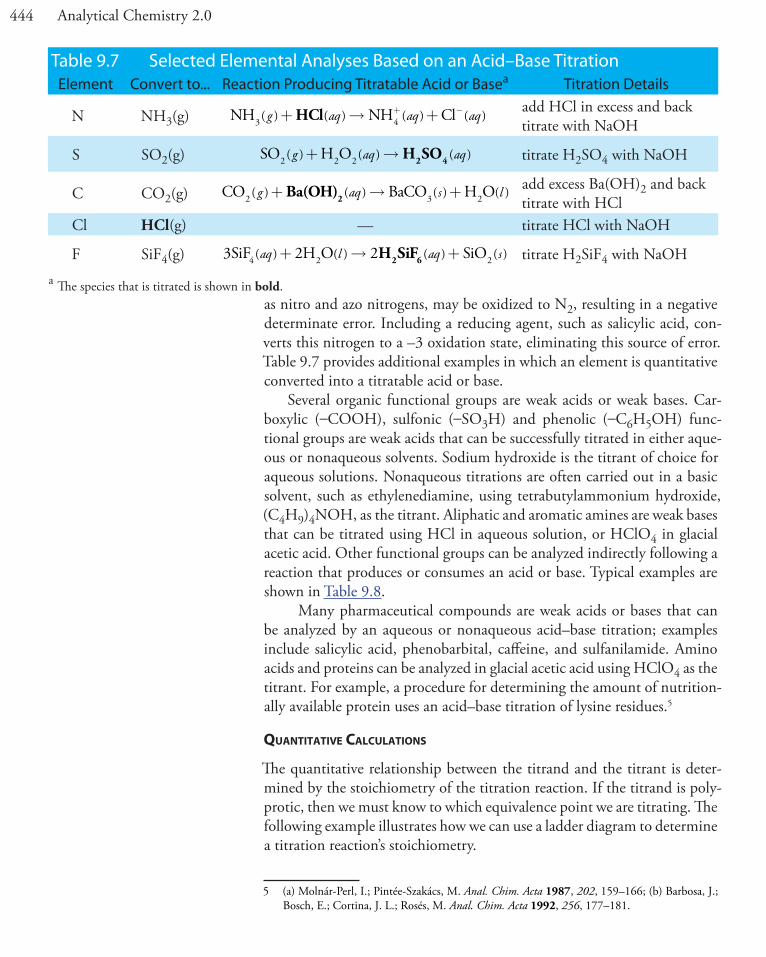
444 Analytical Chemistry 2.0
as nitro and azo nitrogens, may be oxidized to N2, resulting in a negative determinate error. Including a reducing agent, such as salicylic acid, con-verts this nitrogen to a –3 oxidation state, eliminating this source of error. Table 9.7 provides additional examples in which an element is quantitative converted into a titratable acid or base.
Several organic functional groups are weak acids or weak bases. Car-boxylic (–COOH), sulfonic (–SO3H) and phenolic (–C6H5OH) func-tional groups are weak acids that can be successfully titrated in either aque-ous or nonaqueous solvents. Sodium hydroxide is the titrant of choice for aqueous solutions. Nonaqueous titrations are often carried out in a basic solvent, such as ethylenediamine, using tetrabutylammonium hydroxide, (C4H9)4NOH, as the titrant. Aliphatic and aromatic amines are weak bases that can be titrated using HCl in aqueous solution, or HClO4 in glacial acetic acid. Other functional groups can be analyzed indirectly following a reaction that produces or consumes an acid or base. Typical examples are shown in Table 9.8.
Many pharmaceutical compounds are weak acids or bases that can be analyzed by an aqueous or nonaqueous acid–base titration; examples include salicylic acid, phenobarbital, caffeine, and sulfanilamide. Amino acids and proteins can be analyzed in glacial acetic acid using HClO4 as the titrant. For example, a procedure for determining the amount of nutrition-ally available protein uses an acid–base titration of lysine residues.5
quanTiTaTive calculaTionS
The quantitative relationship between the titrand and the titrant is deter-mined by the stoichiometry of the titration reaction. If the titrand is poly-protic, then we must know to which equivalence point we are titrating. The following example illustrates how we can use a ladder diagram to determine a titration reaction’s stoichiometry.
5 (a) Molnár-Perl, I.; Pintée-Szakács, M. Anal. Chim. Acta 1987, 202, 159–166; (b) Barbosa, J.; Bosch, E.; Cortina, J. L.; Rosés, M. Anal. Chim. Acta 1992, 256, 177–181.
Table 9.7 Selected Elemental Analyses Based on an Acid–Base TitrationElement Convert to... Reaction Producing Titratable Acid or Basea Titration Details
N NH3(g) NH NH Cl3 4( ) ( ) ( ) ( )g aq aq aq+ → ++ −HCl add HCl in excess and back titrate with NaOH
S SO2(g) SO H O22 2( ) ( ) ( )g aq aq+ →H SO2 4 titrate H2SO4 with NaOH
C CO2(g) CO BaCO H O22 3( ) ( ) ( ) ( )g aq s l+ → +Ba(OH)2add excess Ba(OH)2 and back titrate with HCl
Cl HCl(g) — titrate HCl with NaOH
F SiF4(g) 3SiF H O SiO24 22 2( ) ( ) ( ) ( )aq l aq s+ → +H SiF2 6 titrate H2SiF4 with NaOHa The species that is titrated is shown in bold.

445Chapter 9 Titrimetric Methods
Example 9.2
A 50.00 mL sample of a citrus drink requires 17.62 mL of 0.04166 M NaOH to reach the phenolphthalein end point. Express the sample’s acid-ity as grams of citric acid, C6H8O7, per 100 mL.
Solution
Because citric acid is a triprotic weak acid, we must first determine if the phenolphthalein end point corresponds to the first, second, or third equiv-alence point. Citric acid’s ladder diagram is shown in Figure 9.20a. Based on this ladder diagram, the first equivalence point is between a pH of 3.13 and a pH of 4.76, the second equivalence point is between a pH of 4.76 and a pH of 6.40, and the third equivalence point is greater than a pH of 6.40. Because phenolphthalein’s end point pH is 8.3–10.0 (see Table 9.4), the titration proceeds to the third equivalence point and the titration reaction is
C H O OH C H O H O6 8 7 6 5 73
2( ) ( ) ( ) ( )aq aq aq l+ → +− −3 3
In reaching the equivalence point, each mole of citric acid consumes three moles of NaOH; thus
0 04166 7 3405 10 5. .M NaOH 0.01762 L NaOH m� = � − ooles NaOH
7 3405 1015. � �− mol NaOH
mol C H O3 mol NaOH
6 8 7
== � −2 4468 10 4. mol C H O6 8 7
Table 9.8 Selected Acid–Base Titrimetric Procedures for Organic Functional Groups Based on the Production or Consumption of Acid or Base
Functional Group Reaction Producing Titratable Acid or Basea Titration Details
ester RCOOR RCOO HOR′ + → + ′−( ) ( ) ( ) ( )aq aq aq aqOH− titrate OH– with HCl
carbonylR C O NH OH HCl
R C NOH2 2
2
= + →
= +
( ) ( )
( ) ( )
aq aq
aq aq
HCl ++H O2 ( )ltitrate HCl with NaOH
alcoholb[ ]
[ ]
1
2
(CH CO) O ROH CH COOR
(CH CO)3 2 3
3 2
+ → +CH COOH3
OO H O2+ → 2CH COOH3
titrate CH3COOH with NaOH; a blank titration of acetic anhydride, (CH3CO)2O, corrects for the contribution of reaction [2]
a The species that is titrated is shown in bold.b The acetylation reaction [1] is carried out in pyridine to prevent the hydrolysis of acetic by water. After the acetylation reaction
is complete, water is added to covert any unreacted acetic anhydride to acetic acid [2].
Figure 9.20 (a) Ladder diagram for citric acid; (b) Titration curve for the sample in Example 9.2 showing phe-nolphthalein’s pH transition region.
more acidic
more basic
pH
pKa1 = 3.13
H3Cit
pKa2 = 4.76
pKa3 = 6.40
H2Cit–
HCit2–
Cit3–(a)
0 5 10 15 20 25 30
0
2
4
6
8
10
12
14
Volume of NaOH (mL)
pH
(b)

446 Analytical Chemistry 2.0
2 4468 10192 134.
.� �− mol C H O
g C H Omol C6 8 7
6 8 7
66 8 76 8 7H O
g C H O= 0 04701.
Because this is the amount of citric acid in a 50.00 mL sample, the concen-tration of citric acid in the citrus drink is 0.09402 g/100 mL. The complete titration curve is shown in Figure 9.20b.
Practice Exercise 9.6Your company recently received a shipment of salicylic acid, C7H6O3, to be used in the production of acetylsalicylic acid (aspirin). The shipment can be accepted only if the salicylic acid is more than 99% pure. To evalu-ate the shipment’s purity, a 0.4208-g sample is dissolved in water and titrated to the phenolphthalein end point, requiring 21.92 mL of 0.1354 M NaOH. Report the shipment’s purity as %w/w C7H6O3. Salicylic acid is a diprotic weak acid with pKa values of 2.97 and 13.74.
Click here to review your answer to this exercise.
In an indirect analysis the analyte participates in one or more prelimi-nary reactions, one of which produces or consumes acid or base. Despite the additional complexity, the calculations are straightforward.
Example 9.3
The purity of a pharmaceutical preparation of sulfanilamide, C6H4N2O2S, is determined by oxidizing sulfur to SO2 and bubbling it through H2O2 to produce H2SO4. The acid is titrated to the bromothymol blue end point with a standard solution of NaOH. Calculate the purity of the preparation given that a 0.5136-g sample requires 48.13 mL of 0.1251 M NaOH.
Solution
The bromothymol blue end point has a pH range of 6.0–7.6. Sulfuric acid is a diprotic acid, with a pKa2 of 1.99 (the first Ka value is very large and the acid dissociation reaction goes to completion, which is why H2SO4 is a strong acid). The titration, therefore, proceeds to the second equivalence point and the titration reaction is
H SO OH H O SO2 4 2( ) ( ) ( ) ( )aq aq l aq+ → +− −2 2 42
Using the titration results, there are
0 1251 0 04813 6 021 10 3. . .M NaOH L NaOH mol� = � − NaOH
6 021 101
33. � � =− mol NaOHmol H SO
2 mol NaOH2 4 ..010 10 3� − mol H SO2 4

447Chapter 9 Titrimetric Methods
produced by bubbling SO2 through H2O2. Because all the sulfur in H2SO4 comes from the sulfanilamide, we can use a conservation of mass to deter-mine the amount of sulfanilamide in the sample.
3 010 101
1
3. � � �− mol H SOmol S
mol H SOmol
2 42 4
C H N O Smol S
g C H N O Smol C H
6 4 2 2 6 4 2 2
6 4
�168 18.
NN O Sg C H N O S
2 2
6 4 2 2= 0 5062.
0 50620 5136
100 98 56.
..
g C H N O Sg sample6 4 2 2 � = %% w/w C H N O S6 4 2 2
Practice Exercise 9.7The concentration of NO2 in air can be determined by passing the sam-ple through a solution of H2O2, which oxidizes NO2 to HNO3, and titrating the HNO3 with NaOH. What is the concentration of NO2, in mg/L, if a 5.0 L sample of air requires 9.14 mL of 0.01012 M NaOH to reach the methyl red end point
Click here to review your answer to this exercise.
For a back titration we must consider two acid–base reactions. Again, the calcula-tions are straightforward.
Example 9.4
The amount of protein in a sample of cheese is determined by a Kjeldahl analysis for nitrogen. After digesting a 0.9814-g sample of cheese, the ni-trogen is oxidized to NH4
+, converted to NH3 with NaOH, and distilled into a collection flask containing 50.00 mL of 0.1047 M HCl. The excess HCl is back titrated with 0.1183 M NaOH, requiring 22.84 mL to reach the bromothymol blue end point. Report the %w/w protein in the cheese assuming that there are 6.38 grams of protein for every gram of nitrogen in most dairy products.
Solution
The HCl in the collection flask reacts with two bases
HCl NH NH Cl4( ) ( ) ( ) ( )aq aq aq aq+ → ++ −3
HCl OH H O Cl2( ) ( ) ( ) ( )aq aq l aq+ → +− −
The collection flask originally contains
0 1047 0 05000 5 235 10 3. . .M HCl L HCl mol H� = � − CCl
of which

448 Analytical Chemistry 2.0
0 1183 0 022841
. .M NaOH L NaOHmol HCl
mol N
� �
aaOHmol HCl= � −2 702 10 3.
react with NaOH. The difference between the total moles of HCl and the moles of HCl reacting with NaOH
5 235 10 2 702 10 2 5333 3. . .� − � =− −mol HCl mol HCl �� −10 3 mol HCl
is the moles of HCl reacting with NH3. Because all the nitrogen in NH3 comes from the sample of cheese, we use a conservation of mass to deter-mine the grams of nitrogen in the sample.
2 533 101 14 013.
.� � �− mol HCl
mol NHmol HCl
g3 Nmol NH
g N3
= 0 03549.
The mass of protein, therefore, is
0 035496 38
0 2264..
.g Ng proteing N
g prot� = eein
and the % w/w protein is
0 2264100 23 1
.. %
g protein0.9814 g sample
w� = //w protein
Practice Exercise 9.8Limestone consists mainly of CaCO3, with traces of iron oxides and other metal oxides. To determine the purity of a limestone, a 0.5413-g sample is dissolved using 10.00 mL of 1.396 M HCl. After heating to expel CO2, the excess HCl was titrated to the phenolphthalein end point, requiring 39.96 mL of 0.1004 M NaOH. Report the sample’s purity as %w/w CaCO3.
Click here to review your answer to this exercise.Earlier we noted that we can use an acid–base titration to analyze a
mixture of acids or bases by titrating to more than one equivalence point. The concentration of each analyte is determined by accounting for its con-tribution to each equivalence point.
Example 9.5
The alkalinity of natural waters is usually controlled by OH–, HCO3–, and
CO32–, which may be present singularly or in combination. Titrating a
100.0-mL sample to a pH of 8.3 requires 18.67 mL of a 0.02812 M HCl. A second 100.0-mL aliquot requires 48.12 mL of the same titrant to reach

449Chapter 9 Titrimetric Methods
a pH of 4.5. Identify the sources of alkalinity and their concentrations in milligrams per liter.
Solution
Because the volume of titrant to reach a pH of 4.5 is more than twice that needed to reach a pH of 8.3, we know, from Table 9.6, that the sample’s alkalinity is controlled by CO3
2– and HCO3–. Titrating to a pH of 8.3
neutralizes CO32– to HCO3
–
CO HCl HCO Cl32
3− − −+ → +( ) ( ) ( ) ( )aq aq aq aq
but there is no reaction between the titrant and HCO3– (see Figure 9.19).
The concentration of CO32– in the sample, therefore, is
0 02812 0 018671 2
. .M HCl L HClmol COmol
3
� �−
HHClmol CO3= � − −5 250 10 4 2.
5 250 100 1000
60 014 2 2..
.��
− − −mol COL
g COm
3 3
ool COmg
gmg/L
32
1000315 1
−� = .
Titrating to a pH of 4.5 neutralizes CO32– to H2CO3, and HCO3
– to H2CO3 (see Figures 9.19).
CO HCl H CO Cl2 332 2 2− −+ → +( ) ( ) ( ) ( )aq aq aq aq
HCO HCl H CO Cl2 33 2− −+ → +( ) ( ) ( ) ( )aq aq aq aq
Because we know how many moles of CO32– are in the sample, we can
calculate the volume of HCl it consumes.
5 250 102
1
4 22
. � � �− −−
mol COmol HCl
mol CO
L
33
HCl0.02812 mol HCl
mLL
mL� =1000
37 34.
This leaves 48.12 mL - 37.34 mL, or 10.78 mL of HCl to react with HCO3
–. The amount of HCO3– in the sample is
0 02812 0 010781
. .M HCl L HClmol HCOmol
3
� �−
HHClmol HCO3= � − −3 031 10 4.
3 031 100 1000
61 024..
.��
− − −mol HCOL
g HCOm
3 3
ool HCOmg
gmg/L
3−� =
1000185 0.

450 Analytical Chemistry 2.0
9B.5 Qualitative Applications
Example 9.5 shows how we can use an acid–base titration to assign the forms of alkalinity in waters. We can easily extend this approach to other systems. For example, by titrating with either a strong acid or a strong base to the methyl orange and phenolphthalein end points we can determine the composition of solutions containing one or two of the following species: H3PO4, H2PO4
–, HPO42–, PO4
3–, HCl, and NaOH. As outlined in Table 9.9, each species or mixture of species has a unique relationship between the volumes of titrant needed to reach these two end points.
9B.6 Characterization Applications
An acid–base titration can be use to characterize the chemical and physi-cal properties of matter. Two useful characterization applications are the
Table 9.9 Relationship Between End Point Volumes for Mixtures of Phosphate Species with HCl and NaOH
Solution Composition Relationship Between End Point Volumes with Strong Base Titranta
Relationship Between End Point Volumes With Strong Acid Titranta
H3PO4 VPH = 2 � VMO —b
H2PO4–
VPH > 0; VMO = 0 —
HPO42– — VMO > 0; VPH = 0
PO43– — VMO = 2 � VPH
HCl VPH = VMO —
NaOH — VMO= VPHHCl and H3PO4 VPH < 2 � VMO —
H3PO4 and H2PO4–
VPH > 2 � VMO —
H2PO4– and HPO4
2–VPH > 0; VMO = 0 VMO > 0; VPH = 0
HPO42– and PO4
3– — VMO > 2 � VPHPO4
3– and NaOH — VMO < 2 � VPHa VPH and VMO are, respectively, the volume of titrant at the phenolphthalein and methyl orange end points.b When no information is provided, the volume of titrant to each end point is zero.
Practice Exercise 9.9Samples containing the monoprotic weak acids 2–methylanilinium chloride (C7H10NCl, pKa = 4.447) and 3–nitrophenol (C6H5NO3, pKa = 8.39) can be analyzed by titrating with NaOH. A 2.006-g sample requires 19.65 mL of 0.200 M NaOH to reach the bromocresol purple end point and 48.41 mL of 0.200 M NaOH to reach the phenolphtha-lein end point. Report the %w/w of each compound in the sample.
Click here to review your answer to this exercise.

451Chapter 9 Titrimetric Methods
determination of a compound’s equivalent weight and its acid or its base dissociation constant.
equivalenT WeighTS
Suppose we titrate a sample containing an impure weak acid to a well-defined end point using a monoprotic strong base as the titrant. If we as-sume that the titration involves the transfer of n protons, then the moles of titrant needed to reach the end point is
moles titrantmoles titrant
moles analyte= �
nmmoles analyte
If we know the analyte’s identity, we can use this equation to determine the amount of analyte in the sample
grams analyte moles titrant1 mole analyte
= �n moles titrant
FW analyte�
where FW is the analyte’s formula weight. But what if we do not know the analyte’s identify? If we can titrate a
pure sample of the analyte, we can obtain some useful information that may help in establishing its identity. Because we do not know the number of protons being titrated, we let n = 1 and replace the analyte’s formula weight with its equivalent weight (EW)
grams analyte moles titrant1 equivalent an
= �aalyte
1 moles titrantEW analyte�
whereFW EW= �n
Example 9.6
A 0.2521-g sample of an unknown weak acid is titrated with 0.1005 M NaOH, requiring 42.68 mL to reach the phenolphthalein end point. De-termine the compound’s equivalent weight. Which of the following com-pounds is most likely to be the unknown weak acid?
ascorbic acid C8H8O6 FW = 176.1 monoprotic
malonic acid C3H4O4 FW = 104.1 diprotic
succinic acid C4H6O4 FW = 118.1 diprotic
citric acid C6H8O7 FW = 192.1 triprotic
Solution
The moles of NaOH needed to reach the end point is

452 Analytical Chemistry 2.0
0 1005 0 04268 4 289 10 3. . .M NaOH L NaOH mol� = � − NaOH
which gives the analyte’s equivalent weight as
EW = =�
g analyteequiv. analyte
g0 25214 289 10
.. −−
=3
58 78equiv.
g/equivalent.
The possible formula weights for the weak acid are
nn= = =
= = � =
1 58 782 2 117
: .:
FW EW g/equivalentFW EW ..
: .6
3 3 176 3g/equivalent
FW EW g/equivaln= = � = eent
If the analyte is a monoprotic weak acid, then its formula weight is 58.78 g/mol, eliminating ascorbic acid as a possibility. If it is a diprotic weak acid, then the analyte’s formula weight is either 58.78 g/mol or 117.6 g/mol, de-pending on whether the titration is to the first or second equivalence point. Succinic acid, with a formula weight of 118.1 g/mole is a possibility, but malonic acid is not. If the analyte is a triprotic weak acid, then its formula weight is 58.78 g/mol, 117.6 g/mol, or 176.3 g/mol. None of these values is close to the formula weight for citric acid, eliminating it as a possibility. Only succinic acid provides a possible match.
Figure 9.21 Titration curve for Practice Exercise 9.10.
Practice Exercise 9.10Figure 9.21 shows the potentiometric titration curve for the titration of a 0.500-g sample an unknown weak acid. The titrant is 0.1032 M NaOH. What is the weak acid’s equivalent weight?
Click here to review your answer to this exercise.
0 20 40 60 80 100 120
0
2
4
6
8
10
12
14
Volume of NaOH (mL)
pH

453Chapter 9 Titrimetric Methods
Figure 9.22 Estimating acetic acid’s pKa using its poten-tiometric titration curve.
Practice Exercise 9.11Use the potentiometric titration curve in Figure 9.21 to estimate the pKa values for the weak acid in Practice Exercise 9.10.
Click here to review your answer to this exercise.
equiliBriuM conSTanTS
Another application of acid–base titrimetry is the determination of equilib-rium constants. Consider, for example, a solution of acetic acid, CH3COOH, for which the dissociation constant is
K a3 3
3
H O CH COOCH COOH
=+ −[ ][ ]
[ ]
When the concentrations of CH3COOH and CH3COO– are equal, the Ka expression reduces to Ka = [H3O+], or pH = pKa. If we titrate a solution of acetic acid with NaOH, the pH equals the pKa when the volume of NaOH is approximately ½Veq. As shown in Figure 9.22, a potentiometric titration curve provides a reasonable estimate of acetic acid’s pKa.
This method provides a reasonable estimate of a weak acid’s pKa if the acid is neither too strong nor too weak. These limitations are easily to ap-preciate if we consider two limiting cases. For the first case let’s assume that the weak acid, HA, is more than 50% dissociated before the titration begins (a relatively large Ka value). The concentration of HA before the equivalence point is always less than the concentration of A–, and there is no point on the titration curve where [HA] = [A–]. At the other extreme, if the acid is too weak, less than 50% of the weak acid reacts with the titrant at the equivalence point. In this case the concentration of HA before the equivalence point is always greater than that of A–. Determining the pKa by the half-equivalence point method overestimates its value if the acid is too strong and underestimates its value if the acid is too weak.
0 10 20 30 40 50Volume of NaOH (mL)
0
2
4
6
8
10
12
14
pHVeq
½×Veq
pKa
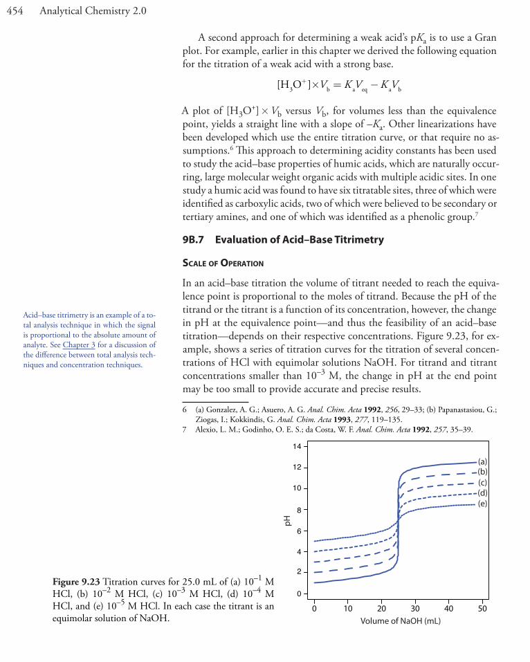
454 Analytical Chemistry 2.0
A second approach for determining a weak acid’s pKa is to use a Gran plot. For example, earlier in this chapter we derived the following equation for the titration of a weak acid with a strong base.
[ ]H O3 b a eq a b+ � = −V K V K V
A plot of [H3O+] � Vb versus Vb, for volumes less than the equivalence point, yields a straight line with a slope of –Ka. Other linearizations have been developed which use the entire titration curve, or that require no as-sumptions.6 This approach to determining acidity constants has been used to study the acid–base properties of humic acids, which are naturally occur-ring, large molecular weight organic acids with multiple acidic sites. In one study a humic acid was found to have six titratable sites, three of which were identified as carboxylic acids, two of which were believed to be secondary or tertiary amines, and one of which was identified as a phenolic group.7
9B.7 Evaluation of Acid–Base Titrimetry
Scale oF oPeraTion
In an acid–base titration the volume of titrant needed to reach the equiva-lence point is proportional to the moles of titrand. Because the pH of the titrand or the titrant is a function of its concentration, however, the change in pH at the equivalence point—and thus the feasibility of an acid–base titration—depends on their respective concentrations. Figure 9.23, for ex-ample, shows a series of titration curves for the titration of several concen-trations of HCl with equimolar solutions NaOH. For titrand and titrant concentrations smaller than 10–3 M, the change in pH at the end point may be too small to provide accurate and precise results.
6 (a) Gonzalez, A. G.; Asuero, A. G. Anal. Chim. Acta 1992, 256, 29–33; (b) Papanastasiou, G.; Ziogas, I.; Kokkindis, G. Anal. Chim. Acta 1993, 277, 119–135.
7 Alexio, L. M.; Godinho, O. E. S.; da Costa, W. F. Anal. Chim. Acta 1992, 257, 35–39.
Figure 9.23 Titration curves for 25.0 mL of (a) 10–1 M HCl, (b) 10–2 M HCl, (c) 10–3 M HCl, (d) 10–4 M HCl, and (e) 10–5 M HCl. In each case the titrant is an equimolar solution of NaOH.
Acid–base titrimetry is an example of a to-tal analysis technique in which the signal is proportional to the absolute amount of analyte. See Chapter 3 for a discussion of the difference between total analysis tech-niques and concentration techniques.
0 10 20 30 40 50
0
2
4
6
8
10
12
14
(a)(b)(c)(d)(e)
Volume of NaOH (mL)
pH

455Chapter 9 Titrimetric Methods
A minimum concentration of 10–3 M places limits on the smallest amount of analyte that we can successfully analyze. For example, suppose our analyte has a formula weight of 120 g/mol. To successfully monitor the titration’s end point using an indicator or with a pH probe, the titrand needs an initial volume of approximately 25 mL. If we assume that the ana-lyte’s formula weight is 120 g/mol, then each sample must contain at least 3 mg of analyte. For this reason, acid–base titrations are generally limited to major and minor analytes (see Figure 3.6 in Chapter 3). We can extend the analysis of gases to trace analytes by pulling a large volume of the gas through a suitable collection solution.
One goal of analytical chemistry is to extend analyses to smaller sam-ples. Here we describe two interesting approaches to titrating mL and pL samples. In one experimental design (Figure 9.24), samples of 20–100 mL were held by capillary action between a flat-surface pH electrode and a stainless steel sample stage.8 The titrant was added by using the oscillations of a piezoelectric ceramic device to move an angled glass rod in and out of a tube connected to a reservoir containing the titrant. Each time the glass tube was withdrawn an approximately 2 nL microdroplet of titrant was released. The microdroplets were allowed to fall onto the sample, with mix-ing accomplished by spinning the sample stage at 120 rpm. A total of 450 microdroplets, with a combined volume of 0.81 –0.84 mL, was dispensed between each pH measurement. In this fashion a titration curve was con-structed. This method was used to titrate solutions of 0.1 M HCl and 0.1 M CH3COOH with 0.1 M NaOH. Absolute errors ranged from a minimum of +0.1% to a maximum of –4.1%, with relative standard deviations from 0.15% to 4.7%. Sample as small as 20 mL were successfully titrated.
8 Steele, A.; Hieftje, G. M. Anal. Chem. 1984, 56, 2884–2888.
Figure 9.24 Experimental design for a microdroplet titration apparatus.
titrant
piezoelectric ceramic
pH electrode
samplerotating
sample stage
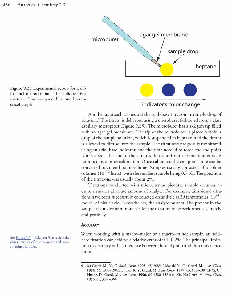
456 Analytical Chemistry 2.0
Another approach carries out the acid–base titration in a single drop of solution.9 The titrant is delivered using a microburet fashioned from a glass capillary micropipet (Figure 9.25). The microburet has a 1-2 mm tip filled with an agar gel membrane. The tip of the microburet is placed within a drop of the sample solution, which is suspended in heptane, and the titrant is allowed to diffuse into the sample. The titration’s progress is monitored using an acid–base indicator, and the time needed to reach the end point is measured. The rate of the titrant’s diffusion from the microburet is de-termined by a prior calibration. Once calibrated the end point time can be converted to an end point volume. Samples usually consisted of picoliter volumes (10–12 liters), with the smallest sample being 0.7 pL. The precision of the titrations was usually about 2%.
Titrations conducted with microliter or picoliter sample volumes re-quire a smaller absolute amount of analyte. For example, diffusional titra-tions have been successfully conducted on as little as 29 femtomoles (10–15 moles) of nitric acid. Nevertheless, the analyte must still be present in the sample at a major or minor level for the titration to be performed accurately and precisely.
accuracy
When working with a macro–major or a macro–minor sample, an acid–base titration can achieve a relative error of 0.1–0.2%. The principal limita-tion to accuracy is the difference between the end point and the equivalence point.
9 (a) Gratzl, M.; Yi, C. Anal. Chem. 1993, 65, 2085–2088; (b) Yi, C.; Gratzl, M. Anal. Chem. 1994, 66, 1976–1982; (c) Hui, K. Y.; Gratzl, M. Anal. Chem. 1997, 69, 695–698; (d) Yi, C.; Huang, D.; Gratzl, M. Anal. Chem. 1996, 68, 1580–1584; (e) Xie, H.; Gratzl, M. Anal. Chem. 1996, 68, 3665–3669.
See Figure 3.5 in Chapter 3 to review the characteristics of macro–major and mac-ro–minor samples.
Figure 9.25 Experimental set-up for a dif-fusional microtitration. The indicator is a mixture of bromothymol blue and bromo-cresol purple.
microburetagar gel membrane
sample drop
heptane
indicator’s color change

457Chapter 9 Titrimetric Methods
PreciSion
An acid–base titration’s relative precision depends primarily on the preci-sion with which we can measure the end point volume and the precision in detecting the end point. Under optimum conditions, an acid–base titration has a relative precision of 0.1–0.2%. We can improve the relative precision by using the largest possible buret and ensuring that we use most of its ca-pacity in reaching the end point. A smaller volume buret is a better choice when using costly reagents, when waste disposal is a concern, or when the titration must be completed quickly to avoid competing chemical reactions. Automatic titrators are particularly useful for titrations requiring small vol-umes of titrant because they provide significantly better precision (typically about ±0.05% of the buret’s volume).
The precision of detecting the end point depends on how it is measured and the slope of the titration curve at the end point. With an indicator the precision of the end point signal is usually ±0.03–0.10 mL. Potentiometric end points usually are more precise.
SenSiTiviTy
For an acid–base titration we can write the following general analytical equation relating the titrant’s volume to the absolute amount of titrand
volume of titrant moles of titrand= �k
where k, the sensitivity, is determined by the stoichiometry between the titrand and the titrant. Consider, for example, the determination of sulfu-rous acid, H2SO3, by titrating with NaOH to the first equivalence point
H SO OH H O HSO2 3 2( ) ( ) ( ) ( )aq aq l aq+ → +− −3
At the equivalence point the relationship between the moles of NaOH and the moles of H2SO3 is
mol NaOH mol H SO2 3=
Substituting the titrant’s molarity and volume for the moles of NaOH and rearranging
M VNaOH NaOH 2 3mol H SO� =
VMNaOH
NaOH2 3mol H SO= �
1
we find that k is
kMNaOH
=1

458 Analytical Chemistry 2.0
There are two ways in which we can improve a titration’s sensitivity. The first, and most obvious, is to decrease the titrant’s concentration because it is inversely proportional to the sensitivity, k.
The second approach, which only applies if the titrand is multiprotic, is to titrate to a later equivalence point. If we titrate H2SO3 to the second equivalence point
H SO OH H O SO2 3 2( ) ( ) ( ) ( )aq aq l aq+ → +− −2 2 32
then each mole of H2SO3 consumes two moles of NaOH
mol NaOH 2 mol H SO2 3= �
and the sensitivity becomes
kMNaOH
=2
In practice, however, any improvement in sensitivity is offset by a de-crease in the end point’s precision if the larger volume of titrant requires us to refill the buret. Consequently, standard acid–base titrimetric proce-dures are written to ensure that titrations require 60–100% of the buret’s volume.
SelecTiviTy
Acid–base titrants are not selective. A strong base titrant, for example, reacts with all acids in a sample, regardless of their individual strengths. If the titrand contains an analyte and an interferent, then selectivity depends on their relative acid strengths. Two limiting situations must be considered.
If the analyte is a stronger acid than the interferent, then the titrant will react with the analyte before it begins reacting with the interferent. The feasibility of the analysis depends on whether the titrant’s reaction with the interferent affects the accurate location of the analyte’s equivalence point. If the acid dissociation constants are substantially different, the end point for the analyte can be accurately determined. Conversely, if the acid dissocia-tion constants for the analyte and interferent are similar, then an accurate end point for the analyte may not be found. In the latter case a quantitative analysis for the analyte is not possible.
In the second limiting situation the analyte is a weaker acid than the interferent. In this case the volume of titrant needed to reach the analyte’s equivalence point is determined by the concentration of both the analyte and the interferent. To account for the interferent’s contribution to the end point, an end point for the interferent must be present. Again, if the acid dissociation constants for the analyte and interferent are significantly different, then the analyte’s determination is possible. If the acid dissocia-tion constants are similar, however, there is only a single equivalence point

459Chapter 9 Titrimetric Methods
and the analyte’s and interferent’s contributions to the equivalence point volume can not be separated.
TiMe, coST, and equiPMenT
Acid–base titrations require less time than most gravimetric procedures, but more time than many instrumental methods of analysis, particularly when analyzing many samples. With an automatic titrator, however, concerns about analysis time are less significant. When performing a titration manu-ally our equipment needs—a buret and, perhaps, a pH meter—are few in number, inexpensive, routinely available, and easy to maintain. Automatic titrators are available for between $3000 and $10 000.
9C Complexation TitrationsThe earliest examples of metal–ligand complexation titrations are Lie-big’s determinations, in the 1850s, of cyanide and chloride using, respec-tively, Ag+ and Hg2+ as the titrant. Practical analytical applications of com-plexation titrimetry were slow to develop because many metals and ligands form a series of metal–ligand complexes. Liebig’s titration of CN– with Ag+ was successful because they form a single, stable complex of Ag(CN)2
–, giving a single, easily identified end point. Other metal–ligand complexes, such as CdI4
2–, are not analytically useful because they form a series of metal–ligand complexes (CdI+, CdI2(aq), CdI3
– and CdI42–) that produce
a sequence of poorly defined end points.In 1945, Schwarzenbach introduced aminocarboxylic acids as multi-
dentate ligands. The most widely used of these new ligands—ethylenedi-aminetetraacetic acid, or EDTA—forms strong 1:1 complexes with many metal ions. The availability of a ligand that gives a single, easily identified end point made complexation titrimetry a practical analytical method.
9C.1 Chemistry and Properties of EDTA
Ethylenediaminetetraacetic acid, or EDTA, is an aminocarboxylic acid. EDTA, which is shown in Figure 9.26a in its fully deprotonated form, is a Lewis acid with six binding sites—four negatively charged carboxylate groups and two tertiary amino groups—that can donate six pairs of elec-trons to a metal ion. The resulting metal–ligand complex, in which EDTA forms a cage-like structure around the metal ion (Figure 9.26b), is very stable. The actual number of coordination sites depends on the size of the metal ion, however, all metal–EDTA complexes have a 1:1 stoichiometry.
Figure 9.26 Structures of (a) EDTA, in its fully depro-tonated form, and (b) in a six-coordinate metal–EDTA complex with a divalent metal ion.
Recall that an acid–base titration curve for a diprotic weak acid has a single end point if its two Ka values are not sufficiently dif-ferent. See Figure 9.11 for an example.
O
O
O
O
O–
O–
O–
O–
M2+N
N
NN
O
−O
O O−
O
O−
O−O
(a)
(b)

460 Analytical Chemistry 2.0
MeTal–edTa ForMaTion conSTanTS
To illustrate the formation of a metal–EDTA complex, let’s consider the reaction between Cd2+ and EDTA
Cd Y CdY2 4 2+ − −+( ) ( ) ( )aq aq aq 9.9
where Y4– is a shorthand notation for the fully deprotonated form of EDTA shown in Figure 9.26a. Because the reaction’s formation constant
K f
CdYCd Y
= = �−
+ −
[ ][ ][ ]
.2
2 4162 9 10 9.10
is large, its equilibrium position lies far to the right. Formation constants for other metal–EDTA complexes are found in Appendix 12.
edTa iS a Weak acid
In addition to its properties as a ligand, EDTA is also a weak acid. The fully protonated form of EDTA, H6Y2+, is a hexaprotic weak acid with succes-sive pKa values of
p p pp p p
a1 a2 a3
a4 a5 a6
K K KK K K= = =
= = =
0 0 1 5 2 02 66 6 16. . .. . 110 24.
The first four values are for the carboxylic acid protons and the last two values are for the ammonium protons. Figure 9.27 shows a ladder diagram for EDTA. The specific form of EDTA in reaction 9.9 is the predominate species only at pH levels greater than 10.17.
condiTional MeTal–ligand ForMaTion conSTanTS
The formation constant for CdY2– in equation 9.10 assumes that EDTA is present as Y4–. Because EDTA has many forms, when we prepare a solution of EDTA we know it total concentration, CEDTA, not the concentration of a specific form, such as Y4–. To use equation 9.10, we need to rewrite it in terms of CEDTA.
At any pH a mass balance on EDTA requires that its total concentration equal the combined concentrations of each of its forms.
CEDTA 6 5 4
3 2
H Y H Y H Y
H Y H Y
= + + +
+ +
+ +
− −
[ ] [ ] [ ]
[ ] [ ] [
2
2 HHY Y3 4− −+] [ ]
To correct the formation constant for EDTA’s acid–base properties we need to calculate the fraction, aY4–, of EDTA present as Y4–.
αY
EDTA
Y4
4
− =−[ ]
C9.11
Figure 9.27 Ladder diagram for EDTA.
10.24
6.16
2.66
2.01.5
0.0
HY3–
H2Y2–
H3Y–
H4Y
H5Y+
H6Y2+
Y4–
pH

461Chapter 9 Titrimetric Methods
Table 9.10 provides values of aY4– for selected pH levels. Solving equation 9.11 for [Y4–] and substituting into equation 9.10 for the CdY2– formation constant
KCf
Y EDTA
CdYCd
=−
+−
[ ][ ]
2
24α
and rearranging gives
K KCf f Y
EDTA
CdYCd
′ = � =−
−
+α 4
2
2
[ ][ ]
9.12
where Kf´ is a pH-dependent conditional formation constant. As shown in Table 9.11, the conditional formation constant for CdY2– be-comes smaller and the complex becomes less stable at more acidic pHs.
edTa coMPeTeS WiTh oTher ligandS
To maintain a constant pH during a complexation titration we usually add a buffering agent. If one of the buffer’s components is a ligand that binds Cd2+, then EDTA must compete with the ligand for Cd2+. For example, an
Table 9.10 Values of aY4– for Selected pH LevelspH aY4– pH aY4–
1 1.9 � 10–18 8 5.6� 10–3
2 3.4 � 10–14 9 5.4 � 10–2
3 2.6 � 10–11 10 0.374 3.8 � 10–9 11 0.855 3.7 � 10–7 12 0.986 2.4 � 10–5 13 1.007 5.0� 10–4 14 1.00
Problem 9.42 from the end of chapter problems asks you to verify the values in Table 9.10 by deriving an equation for aY4-.
Table 9.11 Conditional Formation Constants for CdY2–
pH Kf´ pH Kf´1 5.5� 10–2 8 1.6 � 1014
2 1.0 � 103 9 1.6 � 1015
3 7.7 � 105 10 1.1� 1016
4 1.1 � 108 11 2.5 � 1016
5 1.1 � 1010 12 2.9 � 1016
6 6.8� 1011 13 2.9 � 1016
7 1.5 � 1013 14 2.9 � 1016

462 Analytical Chemistry 2.0
NH4+/NH3 buffer includes NH3, which forms several stable Cd2+–NH3
complexes. Because EDTA forms a stronger complex with Cd2+ it will dis-place NH3, but the stability of the Cd2+–EDTA complex decreases.
We can account for the effect of an auxiliary complexinG aGent, such as NH3, in the same way we accounted for the effect of pH. Before adding EDTA, the mass balance on Cd2+, CCd, is
C NH
NH NHCd Cd Cd
Cd Cd
= + +
+
+ +
+
[ ] [ ( ) ]
[ ( ) ] [ (
23
2
3 22
3 )) ] [ ( ) ]32
3 42+ ++ Cd NH
and the fraction of uncomplexed Cd2+, aCd2+, is
αCd
Cd
2+
Cd=
+[ ]2
C9.13
Solving equation 9.13 for [Cd2+] and substituting into equation 9.12 gives
K KC Cf f Y
Cd Cd EDTA
CdY
2+
′ = � =−
−
αα
4
2[ ]
Because the concentration of NH3 in a buffer is essentially constant, we can rewrite this equation
K KC Cf f Y Cd
Cd EDTA
2+
CdY′′ = � � =−
−
α α4
2[ ]9.14
to give a conditional formation constant, Kf´́ , that accounts for both pH and the auxiliary complexing agent’s concentration. Table 9.12 provides values of aM2+ for several metal ion when NH3 is the complexing agent.
9C.2 Complexometric EDTA Titration Curves
Now that we know something about EDTA’s chemical properties, we are ready to evaluate its usefulness as a titrant. To do so we need to know the
Table 9.12 Values of aM2+ for Selected Concentrations of Ammonia[NH3] (M) aCa2+ aCd2+ aCo2+ aCu2+ aMg2+ aNi2+ aZn2+
1 5.50 � 10–1 6.09 � 10–8 1.00 � 10–6 3.79 � 10–14 1.76 � 10–1 9.20 � 10–10 3.95 � 10–10
0.5 7.36 � 10–1 1.05 � 10–6 2.22 � 10–5 6.86 � 10–13 4.13 � 10–1 3.44 � 10–8 6.27 � 10–9
0.1 9.39 � 10–1 3.51 � 10–4 6.64 � 10–3 4.63 � 10–10 8.48 � 10–1 5.12 � 10–5 3.68 � 10–6
0.05 9.69 � 10–1 2.72 � 10–3 3.54 � 10–2 7.17 � 10–9 9.22 � 10–1 6.37 � 10–4 5.45 � 10–5
0.01 9.94 � 10–1 8.81 � 10–2 3.55 � 10–1 3.22 � 10–6 9.84 � 10–1 4.32 � 10–2 1.82 � 10–2
0.005 9.97 � 10–1 2.27 � 10–1 5.68 � 10–1 3.62 � 10–5 9.92 � 10–1 1.36 � 10–1 1.27 � 10–1
0.001 9.99 � 10–1 6.09 � 10–1 8.84 � 10–1 4.15 � 10–3 9.98 � 10–1 5.76 � 10–1 7.48 � 10–1
The value of aCd2+ depends on the con-centration of NH3. Contrast this with aY4-, which depends on pH.
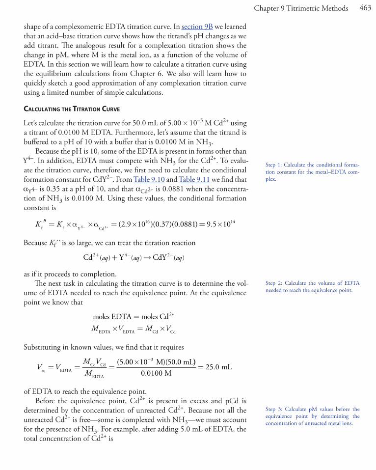
463Chapter 9 Titrimetric Methods
shape of a complexometric EDTA titration curve. In section 9B we learned that an acid–base titration curve shows how the titrand’s pH changes as we add titrant. The analogous result for a complexation titration shows the change in pM, where M is the metal ion, as a function of the volume of EDTA. In this section we will learn how to calculate a titration curve using the equilibrium calculations from Chapter 6. We also will learn how to quickly sketch a good approximation of any complexation titration curve using a limited number of simple calculations.
calculaTing The TiTraTion curve
Let’s calculate the titration curve for 50.0 mL of 5.00 � 10–3 M Cd2+ using a titrant of 0.0100 M EDTA. Furthermore, let’s assume that the titrand is buffered to a pH of 10 with a buffer that is 0.0100 M in NH3.
Because the pH is 10, some of the EDTA is present in forms other than Y4–. In addition, EDTA must compete with NH3 for the Cd2+. To evalu-ate the titration curve, therefore, we first need to calculate the conditional formation constant for CdY2–. From Table 9.10 and Table 9.11 we find that aY4– is 0.35 at a pH of 10, and that aCd2+ is 0.0881 when the concentra-tion of NH3 is 0.0100 M. Using these values, the conditional formation constant is
K Kf f Y Cd2+′′ = � � = �−α α4 2 9 10 0 37 0 088116( . )( . )( . )== �9 5 1014.
Because Kf´́ is so large, we can treat the titration reaction
Cd Y CdY2 4 2+ − −+ →( ) ( ) ( )aq aq aq
as if it proceeds to completion.The next task in calculating the titration curve is to determine the vol-
ume of EDTA needed to reach the equivalence point. At the equivalence point we know that
moles EDTA moles Cd2+
EDTA EDTA Cd Cd
=� = �M V M V
Substituting in known values, we find that it requires
V VM VMeq EDTA
Cd Cd
EDTA
M)(50.0 mL= = =
� −( .5 00 10 3 ))0.0100 M
mL= 25 0.
of EDTA to reach the equivalence point.Before the equivalence point, Cd2+ is present in excess and pCd is
determined by the concentration of unreacted Cd2+. Because not all the unreacted Cd2+ is free—some is complexed with NH3—we must account for the presence of NH3. For example, after adding 5.0 mL of EDTA, the total concentration of Cd2+ is
Step 1: Calculate the conditional forma-tion constant for the metal–EDTA com-plex.
Step 2: Calculate the volume of EDTA needed to reach the equivalence point.
Step 3: Calculate pM values before the equivalence point by determining the concentration of unreacted metal ions.

464 Analytical Chemistry 2.0
CCd
2initial moles Cd moles EDTA addedtota
=−+
ll volumeCd Cd EDTA EDTA
Cd EDTA
=−
+
=�
M V M VV V
( .5 00 110 3− −M)(50.0 mL) (0.0100 M)(5.0 mL)50.0 mL mL
M+
= � −
5 03 64 10 3
..
To calculate the concentration of free Cd2+ we use equation 9.13
[ ] ( . )( . .Cd M)Cd Cd2+
2 40 0881 3 64 10 3 21+ −= � = � =α C �� −10 4 M
which gives a pCd of
pCd Cd=− =− � =+ −log[ ] log( . ) .2 43 21 10 3 49
At the equivalence point all the Cd2+ initially in the titrand is now pres-ent as CdY2–. The concentration of Cd2+, therefore, is determined by the dissociation of the CdY2– complex. First, we calculate the concentration of CdY2–.
[ ]CdYinitial moles Cd
total volume
2+Cd2− = =
M VCCd
Cd EDTA
M)(50.0 mL)mL
V V+
=� −( ..
5 00 1050 0
3
++= � −
25 03 33 10 3
..
mLM
Next, we solve for the concentration of Cd2+ in equilibrium with CdY2–.
KC C
xx xf
Cd EDTA
CdY′′ = =� −
= �− −[ ] .
( )( ).
2 33 33 109 5 11014
x C= = � −Cd M1 9 10 9.
Once again, to find the concentration of uncomplexed Cd2+ we must ac-count for the presence of NH3; thus
[ ] ( . )( . .Cd M)Cd Cd2+
2 90 0881 1 9 10 1 70+ −= � = � = �α C 110 10− M
and pCd is 9.77 at the equivalence point.After the equivalence point, EDTA is in excess and the concentration of
Cd2+ is determined by the dissociation of the CdY2– complex. First, we cal-culate the concentrations of CdY2– and of unreacted EDTA. For example, after adding 30.0 mL of EDTA
[ ]CdYinitial moles Cd
total volume
2+Cd2− = =
M VCCd
Cd EDTA
M)(50.0 mL)mL
V V+
=� −( ..
5 00 1050 0
3
++= � −
30 03 13 10 3
..
mLM
Step 4: Calculate pM at the equivalence point using the conditional formation constant.
Step 5: Calculate pM after the equivalence point using the conditional formation constant.
At the equivalence point the initial moles of Cd2+ and the moles of EDTA added are equal. The total concentrations of Cd2+, CCd, and the total concentration of EDTA, CEDTA, are equal.
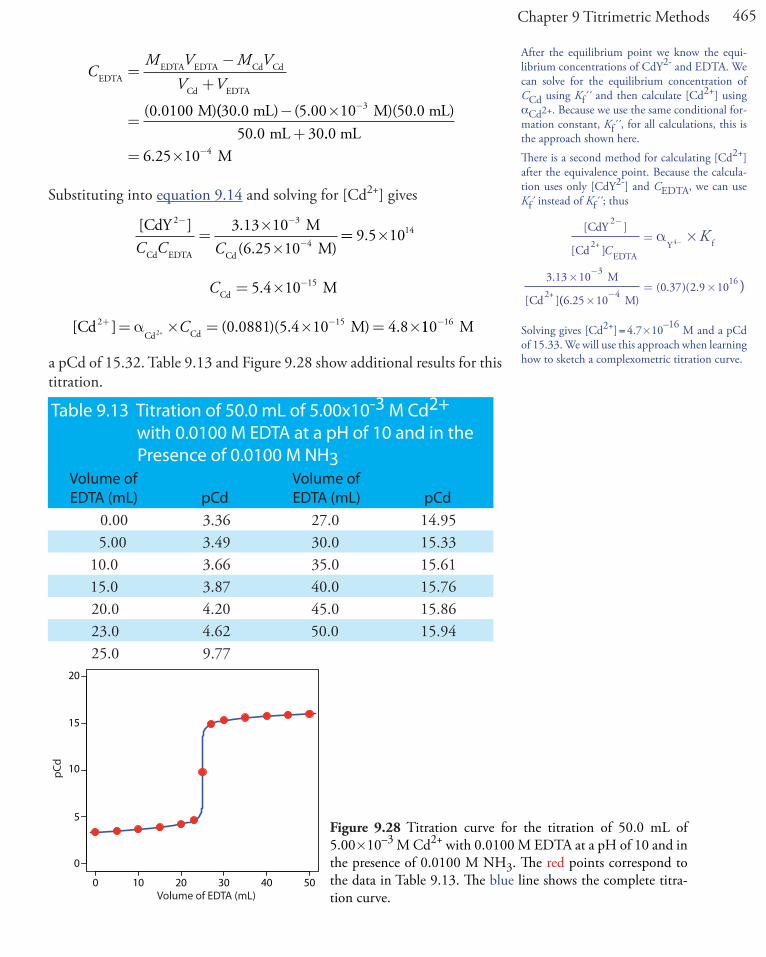
465Chapter 9 Titrimetric Methods
CM V M V
V VEDTAEDTA EDTA Cd Cd
Cd EDTA
M)
=−
+
=( .0 0100 ((30.0 mL) (5.00 M)(50.0 mL)
mL 30− �+
−1050 0
3
. ..0 mLM= � −6 25 10 4.
Substituting into equation 9.14 and solving for [Cd2+] gives
[ ] .( .
CdY MM)Cd EDTA Cd
2 3
4
3 13 106 25 10
− −
−=
��C C C
== �9 5 1014.
CCd M= � −5 4 10 15.
[ ] ( . )( . .Cd M)Cd Cd2+
2 150 0881 5 4 10 4 8+ −= � = � = �α C 110 16− M
a pCd of 15.32. Table 9.13 and Figure 9.28 show additional results for this titration.
Table 9.13 Titration of 50.0 mL of 5.00x10⁻³ M Cd2+ with 0.0100 M EDTA at a pH of 10 and in the Presence of 0.0100 M NH3
Volume of EDTA (mL) pCd
Volume of EDTA (mL) pCd
0.00 3.36 27.0 14.955.00 3.49 30.0 15.33
10.0 3.66 35.0 15.6115.0 3.87 40.0 15.7620.0 4.20 45.0 15.8623.0 4.62 50.0 15.9425.0 9.77
Figure 9.28 Titration curve for the titration of 50.0 mL of 5.00�10–3 M Cd2+ with 0.0100 M EDTA at a pH of 10 and in the presence of 0.0100 M NH3. The red points correspond to the data in Table 9.13. The blue line shows the complete titra-tion curve.
After the equilibrium point we know the equi-librium concentrations of CdY2- and EDTA. We can solve for the equilibrium concentration of CCd using Kf´́ and then calculate [Cd2+] using aCd2+. Because we use the same conditional for-mation constant, Kf´́ , for all calculations, this is the approach shown here.
There is a second method for calculating [Cd2+] after the equivalence point. Because the calcula-tion uses only [CdY2-] and CEDTA, we can use Kf ́instead of Kf´́ ; thus
[ ]
[ ]
.
[ ]
CdY
Cd
M
Cd
2+EDTA
Y f
2+
2
3
4
3 13 10
−
−
=
�
− �C
Kα
(( .( . )( . )
6 25 100 37 2 9 10
416
�= �
− M)
Solving gives [Cd2+] = 4.7�10–16 M and a pCd of 15.33. We will use this approach when learning how to sketch a complexometric titration curve.
0 10 20 30 40 50
0
5
10
15
20
Volume of EDTA (mL)
pCd

466 Analytical Chemistry 2.0
Practice Exercise 9.12Calculate titration curves for the titration of 50.0 mL of 5.00�10–3 M Cd2+ with 0.0100 M EDTA (a) at a pH of 10 and (b) at a pH of 7. Neither titration includes an auxiliary complexing agent. Compare your results with Figure 9.28 and comment on the effect of pH and of NH3 on the titration of Cd2+ with EDTA.
Click here to review your answer to this exercise.
This is the same example that we used in developing the calculations for a complex-ation titration curve. You can review the results of that calculation in Table 9.13 and Figure 9.28.
See Table 9.13 for the values.
See the side bar comment on the previ-ous page for an explanation of why we are ignoring the effect of NH3 on the concen-tration of Cd2+.
SkeTching an edTa TiTraTion curve
To evaluate the relationship between a titration’s equivalence point and its end point, we need to construct only a reasonable approximation of the exact titration curve. In this section we demonstrate a simple method for sketching a complexation titration curve. Our goal is to sketch the titration curve quickly, using as few calculations as possible. Let’s use the titration of 50.0 mL of 5.00�10–3 M Cd2+ with 0.0100 M EDTA in the presence of 0.0100 M NH3 to illustrate our approach.
We begin by calculating the titration’s equivalence point volume, which, as we determined earlier, is 25.0 mL. Next, we draw our axes, placing pCd on the y-axis and the titrant’s volume on the x-axis. To indicate the equiva-lence point’s volume, we draw a vertical line corresponding to 25.0 mL of EDTA. Figure 9.29a shows the result of the first step in our sketch.
Before the equivalence point, Cd2+ is present in excess and pCd is determined by the concentration of unreacted Cd2+ . Because not all the unreacted Cd2+ is free—some is complexed with NH3—we must account for the presence of NH3. The calculations are straightforward, as we saw earlier. Figure 9.29b shows the pCd after adding 5.00 mL and 10.0 mL of EDTA.
The third step in sketching our titration curve is to add two points after the equivalence point. Here the concentration of Cd2+ is controlled by the dissociation of the Cd2+–EDTA complex. Beginning with the conditional formation constant
KC
Kf 2+EDTA
Y f
CdYCd
′ = = � = �−
−
[ ][ ]
( . )( .2
4 0 37 2 9 1α 00 1 1 1016 16) .= �
we take the log of each side and rearrange, arriving at
log log[ ] log[ ]
KCEDTA
f CdCdY′ =− ++
−2
2
pCdCdYf= ′ +
−log log
[ ]K
CEDTA2
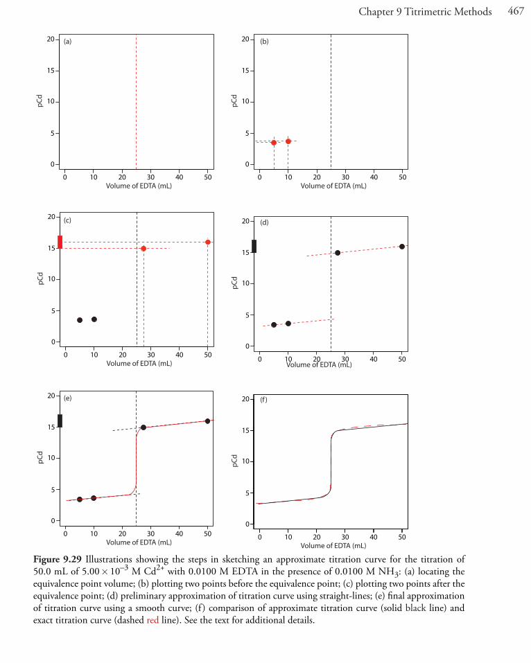
467Chapter 9 Titrimetric Methods
Figure 9.29 Illustrations showing the steps in sketching an approximate titration curve for the titration of 50.0 mL of 5.00 � 10–3 M Cd2+ with 0.0100 M EDTA in the presence of 0.0100 M NH3: (a) locating the equivalence point volume; (b) plotting two points before the equivalence point; (c) plotting two points after the equivalence point; (d) preliminary approximation of titration curve using straight-lines; (e) final approximation of titration curve using a smooth curve; (f ) comparison of approximate titration curve (solid black line) and exact titration curve (dashed red line). See the text for additional details.
0 10 20 30 40 50
0
5
10
15
20
Volume of EDTA (mL)
pCd
(a) (b)
(c)
0 10 20 30 40 50
0
5
10
15
20
Volume of EDTA (mL)
pCd
0 10 20 30 40 50
0
5
10
15
20
Volume of EDTA (mL)
pCd
Volume of EDTA (mL)
(d)
0 10 20 30 40 50
0
5
10
15
20
pCd
(e) (f )
0 10 20 30 40 50
0
5
10
15
20
Volume of EDTA (mL)
pCd
0 10 20 30 40 50
0
5
10
15
20
Volume of EDTA (mL)
pCd

468 Analytical Chemistry 2.0
Note that after the equivalence point, the titrand’s solution is a metal–ligand complexation buffer, with pCd determined by CEDTA and [CdY2–]. The buffer is at its lower limit of pCd = logKf´ – 1 when
CEDTA
CdYmoles EDTA added initial moles
[ ]2−=
− Cdinitial moles Cd
2+
2+=
110
Making appropriate substitutions and solving, we find that
M V M VM V
EDTA EDTA Cd Cd
Cd Cd
−=
110
M V M V M VEDTA EDTA Cd Cd Cd Cd− = �0 1.
VM V
MVEDTA
Cd Cd
EDTAeq=
�= �
1 11 1
..
Thus, when the titration reaches 110% of the equivalence point volume, pCd is logKf´ – 1. A similar calculation should convince you that pCd = logKf´ when the volume of EDTA is 2�Veq.
Figure 9.29c shows the third step in our sketch. First, we add a ladder diagram for the CdY2– complex, including its buffer range, using its logKf´ value of 16.04. Next, we add points representing pCd at 110% of Veq (a pCd of 15.04 at 27.5 mL) and at 200% of Veq (a pCd of 16.04 at 50.0 mL).
Next, we draw a straight line through each pair of points, extending the line through the vertical line representing the equivalence point’s volume (Figure 9.29d). Finally, we complete our sketch by drawing a smooth curve that connects the three straight-line segments (Figure 9.29e). A comparison of our sketch to the exact titration curve (Figure 9.29f ) shows that they are in close agreement.
Our derivation here is general and ap-plies to any complexation titration using EDTA as a titrant.
Practice Exercise 9.13Sketch titration curves for the titration of 50.0 mL of 5.00�10–3 M Cd2+ with 0.0100 M EDTA (a) at a pH of 10 and (b) at a pH of 7. Compare your sketches to the calculated titration curves from Practice Exercise 9.12.
Click here to review your answer to this exercise.
9C.3 Selecting and Evaluating the End point
The equivalence point of a complexation titration occurs when we react stoichiometrically equivalent amounts of titrand and titrant. As is the case with acid–base titrations, we estimate the equivalence point of a complex-ation titration using an experimental end point. A variety of methods are

469Chapter 9 Titrimetric Methods
available for locating the end point, including indicators and sensors that respond to a change in the solution conditions.
Finding The end PoinT WiTh an indicaTor
Most indicators for complexation titrations are organic dyes—known as metallochromic indicators—that form stable complexes with metal ions. The indicator, Inm–, is added to the titrand’s solution where it forms a stable complex with the metal ion, MInn–. As we add EDTA it reacts first with free metal ions, and then displaces the indicator from MInn–.
MIn Y MY Inn m− − − −+ → +4 2
If MInn– and Inm– have different colors, then the change in color signals the end point.
The accuracy of an indicator’s end point depends on the strength of the metal–indicator complex relative to that of the metal–EDTA complex. If the metal–indicator complex is too strong, the change in color occurs after the equivalence point. If the metal–indicator complex is too weak, however, the end point occurs before we reach the equivalence point.
Most metallochromic indicators also are weak acids. One consequence of this is that the conditional formation constant for the metal–indicator complex depends on the titrand’s pH. This provides some control over an indicator’s titration error because we can adjust the strength of a metal–indicator complex by adjusted the pH at which we carry out the titration. Unfortunately, because the indicator is a weak acid, the color of the un-complexed indicator also changes with pH. Figure 9.30, for example, shows the color of the indicator calmagite as a function of pH and pMg, where H2In–, HIn2–, and In3– are different forms of the uncomplexed indicator, and MgIn– is the Mg2+–calmagite complex. Because the color of calmag-ite’s metal–indicator complex is red, it use as a metallochromic indicator has a practical pH range of approximately 8.5–11 where the uncomplexed indicator, HIn2–, has a blue color.
Table 9.14 provides examples of metallochromic indicators and the metal ions and pH conditions for which they are useful. Even if a suitable indicator does not exist, it is often possible to complete an EDTA titration
Table 9.14 Selected Metallochromic IndicatorsIndicator pH Range Metal Ionsa
calmagite 8.5–11 Ba, Ca, Mg, Zneriochrome Black T 7.5–10.5 Ba, Ca, Mg, Zneriochrome Blue Black R 8–12 Ca, Mg, Zn, Cumurexide 6–13 Ca, Ni, CuPAN 2–11 Cd, Cu, Znsalicylic acid 2–3 Fe
a metal ions in italic font have poor end points
Figure 9.30 is essentially a two-variable ladder diagram. The solid lines are equiva-lent to a step on a conventional ladder dia-gram, indicating conditions where two (or three) species are equal in concentration.
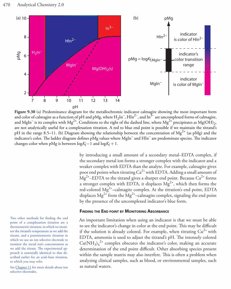
470 Analytical Chemistry 2.0
by introducing a small amount of a secondary metal–EDTA complex, if the secondary metal ion forms a stronger complex with the indicator and a weaker complex with EDTA than the analyte. For example, calmagite gives poor end points when titrating Ca2+ with EDTA. Adding a small amount of Mg2+–EDTA to the titrand gives a sharper end point. Because Ca2+ forms a stronger complex with EDTA, it displaces Mg2+, which then forms the red-colored Mg2+–calmagite complex. At the titration’s end point, EDTA displaces Mg2+ from the Mg2+–calmagite complex, signaling the end point by the presence of the uncomplexed indicator’s blue form.
Finding The end PoinT By MoniToring aBSorBance
An important limitation when using an indicator is that we must be able to see the indicator’s change in color at the end point. This may be difficult if the solution is already colored. For example, when titrating Cu2+ with EDTA, ammonia is used to adjust the titrand’s pH. The intensely colored Cu(NH3)4
2+ complex obscures the indicator’s color, making an accurate determination of the end point difficult. Other absorbing species present within the sample matrix may also interfere. This is often a problem when analyzing clinical samples, such as blood, or environmental samples, such as natural waters.
Two other methods for finding the end point of a complexation titration are a thermometric titration, in which we moni-tor the titrand’s temperature as we add the titrant, and a potentiometric titration in which we use an ion selective electrode to monitor the metal ion’s concentration as we add the titrant. The experimental ap-proach is essentially identical to that de-scribed earlier for an acid–base titration, to which you may refer.
See Chapter 11 for more details about ion selective electrodes.
Figure 9.30 (a) Predominance diagram for the metallochromic indicator calmagite showing the most important form and color of calmagite as a function of pH and pMg, where H2In–, HIn2–, and In3– are uncomplexed forms of calmagite, and MgIn– is its complex with Mg2+. Conditions to the right of the dashed line, where Mg2+ precipitates as Mg(OH)2, are not analytically useful for a complexation titration. A red to blue end point is possible if we maintain the titrand’s pH in the range 8.5–11. (b) Diagram showing the relationship between the concentration of Mg2+ (as pMg) and the indicator’s color. The ladder diagram defines pMg values where MgIn– and HIn– are predominate species. The indicator changes color when pMg is between logKf – 1 and logKf + 1.
(a) (b)
7 8 9 10 11 12 13 14
2
4
6
8
10
MgIn–
H2In–
HIn2–
In3–
pH
pMg
Mg(OH)2(s)
HIn2–
MgIn–
pMg = logKf,MgIn–indicator’s
color transitionrange
indicatoris color of HIn2–
indicatoris color of MgIn–
pMg

471Chapter 9 Titrimetric Methods
Figure 9.31 Examples of spectrophotometric titration curves: (a) only the titrand absorbs; (b) only the titrant absorbs; (c) only the product of the titration reaction absorbs; (d) both the titrand and the titrant absorb; (e) both the titration reaction’s product and the titrant absorb; (f ) only the indicator absorbs. The red arrows indicate the end points for each titration curve.
If at least one species in a complexation titration absorbs electromag-netic radiation, we can identify the end point by monitoring the titrand’s absorbance at a carefully selected wavelength. For example, we can identify the end point for a titration of Cu2+ with EDTA, in the presence of NH3 by monitoring the titrand’s absorbance at a wavelength of 745 nm, where the Cu(NH3)4
2+ complex absorbs strongly. At the beginning of the titration the absorbance is at a maximum. As we add EDTA, however, the reaction
Cu(NH ) Y CuY NH3 42 4 2
34+ − −+ → +( ) ( ) ( ) ( )aq aq aq aq
decreases the concentration of Cu(NH3)42+ and decreases the absorbance
until we reach the equivalence point. After the equivalence point the absor-bance remains essentially unchanged. The resulting spectrophotometric titration curve is shown in Figure 9.31a. Note that the titration curve’s y-axis is not the actual absorbance, A, but a corrected absorbance, Acorr
A AV V
VcorrEDTA Cu
Cu
= �+
where VEDTA and VCu are, respectively, the volumes of EDTA and Cu. Cor-recting the absorbance for the titrand’s dilution ensures that the spectropho-tometric titration curve consists of linear segments that we can extrapolate to find the end point. Other common spectrophotometric titration curves are shown in Figures 9.31b-f.
Aco
rr
Volume of Titrant
(a)
Aco
rr
Volume of Titrant
(b)
Aco
rr
Volume of Titrant
(c)
Aco
rr
Volume of Titrant
(d)
Aco
rr
Volume of Titrant
(e)
Aco
rr
Volume of Titrant
(f )
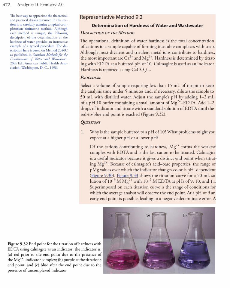
472 Analytical Chemistry 2.0
Representative Method 9.2Determination of Hardness of Water and Wastewater
Description of the MethoD
The operational definition of water hardness is the total concentration of cations in a sample capable of forming insoluble complexes with soap. Although most divalent and trivalent metal ions contribute to hardness, the most important are Ca2+ and Mg2+. Hardness is determined by titrat-ing with EDTA at a buffered pH of 10. Calmagite is used as an indicator. Hardness is reported as mg CaCO3/L.
proceDure
Select a volume of sample requiring less than 15 mL of titrant to keep the analysis time under 5 minutes and, if necessary, dilute the sample to 50 mL with distilled water. Adjust the sample’s pH by adding 1–2 mL of a pH 10 buffer containing a small amount of Mg2+–EDTA. Add 1–2 drops of indicator and titrate with a standard solution of EDTA until the red-to-blue end point is reached (Figure 9.32).
Questions
1. Why is the sample buffered to a pH of 10? What problems might you expect at a higher pH or a lower pH?
Of the cations contributing to hardness, Mg2+ forms the weakest complex with EDTA and is the last cation to be titrated. Calmagite is a useful indicator because it gives a distinct end point when titrat-ing Mg2+. Because of calmagite’s acid–base properties, the range of pMg values over which the indicator changes color is pH–dependent (Figure 9.30). Figure 9.33 shows the titration curve for a 50-mL so-lution of 10–3 M Mg2+ with 10–2 M EDTA at pHs of 9, 10, and 11. Superimposed on each titration curve is the range of conditions for which the average analyst will observe the end point. At a pH of 9 an early end point is possible, leading to a negative determinate error. A
Figure 9.32 End point for the titration of hardness with EDTA using calmagite as an indicator; the indicator is: (a) red prior to the end point due to the presence of the Mg2+–indicator complex; (b) purple at the titration’s end point; and (c) blue after the end point due to the presence of uncomplexed indicator.
The best way to appreciate the theoretical and practical details discussed in this sec-tion is to carefully examine a typical com-plexation titrimetric method. Although each method is unique, the following description of the determination of the hardness of water provides an instructive example of a typical procedure. The de-scription here is based on Method 2340C as published in Standard Methods for the Examination of Water and Wastewater, 20th Ed., American Public Health Asso-ciation: Washington, D. C., 1998.

473Chapter 9 Titrimetric Methods
9C.4 Quantitative Applications
Although many quantitative applications of complexation titrimetry have been replaced by other analytical methods, a few important applications continue to be relevant. In the section we review the general application of complexation titrimetry with an emphasis on applications from the analysis of water and wastewater. First, however, we discuss the selection and stan-dardization of complexation titrants.
SelecTion and STandardizaTion oF TiTranTS
EDTA is a versatile titrant that can be used to analyze virtually all metal ions. Although EDTA is the usual titrant when the titrand is a metal ion, it cannot be used to titrate anions. In the later case, Ag+ or Hg2+ are suitable titrants.
Solutions of EDTA are prepared from its soluble disodium salt, Na2H2Y•2H2O and standardized by titrating against a solution made from the primary standard CaCO3. Solutions of Ag+ and Hg2+ are prepared us-ing AgNO3 and Hg(NO3)2, both of which are secondary standards. Stan-dardization is accomplished by titrating against a solution prepared from primary standard grade NaCl.
late end point and a positive determinate error are possible if we use a pH of 11.
2. Why is a small amount of the Mg2+–EDTA complex added to the buffer?
The titration’s end point is signaled by the indicator calmagite. The indicator’s end point with Mg2+ is distinct, but its change in color when titrating Ca2+ does not provide a good end point. If the sample does not contain any Mg2+ as a source of hardness, then the titra-tion’s end point is poorly defined, leading to inaccurate and imprecise results.
Adding a small amount of Mg2+–EDTA to the buffer ensures that the titrand includes at least some Mg2+. Because Ca2+ forms a stron-ger complex with EDTA, it displaces Mg2+ from the Mg2+–EDTA complex, freeing the Mg2+ to bind with the indicator. This displace-ment is stoichiometric, so the total concentration of hardness cations remains unchanged. The displacement by EDTA of Mg2+ from the Mg2+–indicator complex signals the titration’s end point.
3. Why does the procedure specify that the titration take no longer than 5 minutes?
A time limitation suggests that there is a kinetically controlled inter-ference, possibly arising from a competing chemical reaction. In this case the interference is the possible precipitation of CaCO3 at a pH of 10.
Figure 9.33 Titration curves for 50 mL of 10–3 M Mg2+ with 10–3 M EDTA at pHs 9, 10, and 11 using calmagite as an indicator. The range of pMg and volume of EDTA over which the indi-cator changes color is shown for each titration curve.
0 2 4 6 8 10
0
2
4
6
8
10
Volume of EDTA (mL)
pMg
0 2 4 6 8 10
0
2
4
6
8
10
Volume of EDTA (mL)
pMg
0 2 4 6 8 10
0
2
4
6
8
10
Volume of EDTA (mL)
pMg
early end point
late end point
pH 9
pH 10
pH 11

474 Analytical Chemistry 2.0
inorganic analySiS
Complexation titrimetry continues to be listed as a standard method for the determination of hardness, Ca2+, CN–, and Cl– in waters and waste-waters. The evaluation of hardness was described earlier in Representative Method 9.2. The determination of Ca2+ is complicated by the presence of Mg2+, which also reacts with EDTA. To prevent an interference the pH is adjusted to 12–13, precipitating Mg2+ as Mg(OH)2. Titrating with EDTA using murexide or Eriochrome Blue Black R as the indicator gives the concentration of Ca2+.
Cyanide is determined at concentrations greater than 1 mg/L by mak-ing the sample alkaline with NaOH and titrating with a standard solution of AgNO3, forming the soluble Ag(CN)2
– complex. The end point is de-termined using p-dimethylaminobenzalrhodamine as an indicator, with the solution turning from a yellow to a salmon color in the presence of excess Ag+.
Chloride is determined by titrating with Hg(NO3)2, forming HgCl2(aq). The sample is acidified to a pH of 2.3–3.8 and diphenylcarbazone, which forms a colored complex with excess Hg2+, serves as the indicator. A pH indicator—xylene cyanol FF—is added to ensure that the pH is within the desired range. The initial solution is a greenish blue, and the titration is carried out to a purple end point.
quanTiTaTive calculaTionS
The quantitative relationship between the titrand and the titrant is deter-mined by the stoichiometry of the titration reaction. For a titration using EDTA, the stoichiometry is always 1:1.
Example 9.7
The concentration of a solution of EDTA was determined by standardizing against a solution of Ca2+ prepared using a primary standard of CaCO3. A 0.4071-g sample of CaCO3 was transferred to a 500-mL volumetric flask, dissolved using a minimum of 6 M HCl, and diluted to volume. After transferring a 50.00-mL portion of this solution to a 250-mL Erlenmeyer flask, the pH was adjusted by adding 5 mL of a pH 10 NH3–NH4Cl buf-fer containing a small amount of Mg2+–EDTA. After adding calmagite as an indicator, the solution was titrated with the EDTA, requiring 42.63 mL to reach the end point. Report the molar concentration of EDTA in the titrant.
Solution
The primary standard of Ca2+ has a concentration of
0 4071 1100 09
..
g CaCO0.5000 L
mol Cag C
32+
�aaCO
M Ca3
2+= � −8 135 10 3.
Note that in this example, the analyte is the titrant.

475Chapter 9 Titrimetric Methods
The moles of Ca2+ in the titrand is
8 135 10 0 05000 4 068 103 4. . .� � = �− −M Ca L Ca2+ 2+ mol Ca2+
which means that 4.068�10–4 moles of EDTA are used in the titration. The molarity of EDTA in the titrant is
4 068 109 543 10
4..
�= �
−−mol EDTA
0.04263 L EDTA33 M EDTA
Practice Exercise 9.14A 100.0-mL sample is analyzed for hardness using the procedure out-lined in Representative Method 9.2, requiring 23.63 mL of 0.0109 M EDTA. Report the sample’s hardness as mg CaCO3/L.
Click here to review your answer to this exercise.
Practice Exercise 9.15A 0.4482-g sample of impure NaCN is titrated with 0.1018 M AgNO3, requi i iring 39.68 mL to reach the end point. Report the purity of the sample as %w/w NaCN.
Click here to review your answer to this exercise.
As shown in the following example, we can easily extended this calcula-tion to complexation reactions using other titrants.
Example 9.8
The concentration of Cl– in a 100.0-mL sample of water from a fresh-water aquifer was tested for the encroachment of sea water by titrating with 0.0516 M Hg(NO3)2. The sample was acidified and titrated to the diphenylcarbazone end point, requiring 6.18 mL of the titrant. Report the concentration of Cl–, in mg/L, in the aquifer.
Solution The reaction between Cl– and Hg2+ produces a metal–ligand complex of HgCl2(aq). Each mole of Hg2+ reacts with 2 moles of Cl–; thus
0 05160 00618
2
..
mol Hg(NO )L
L Hg(NO )
m
3 23 2�
�ool Cl
mol Hg(NO )g Cl
mol Cl3 2
− −
−� =
35 4530 0
.. 2226 g Cl−
are in the sample. The concentration of Cl– in the sample is
0 02260 1000
1000226
..
/g Cl
Lmg
gmg L
−
� =
476 Analytical Chemistry 2.0
Finally, complex titrations involving multiple analytes or back titra-tions are possible.
Example 9.9
An alloy of chromel containing Ni, Fe, and Cr was analyzed by a complex-ation titration using EDTA as the titrant. A 0.7176-g sample of the alloy was dissolved in HNO3 and diluted to 250 mL in a volumetric flask. A 50.00-mL aliquot of the sample, treated with pyrophosphate to mask the Fe and Cr, required 26.14 mL of 0.05831 M EDTA to reach the murexide end point. A second 50.00-mL aliquot was treated with hexamethylenete-tramine to mask the Cr. Titrating with 0.05831 M EDTA required 35.43 mL to reach the murexide end point. Finally, a third 50.00-mL aliquot was treated with 50.00 mL of 0.05831 M EDTA, and back titrated to the murexide end point with 6.21 mL of 0.06316 M Cu2+. Report the weight percents of Ni, Fe, and Cr in the alloy.
Solution
The stoichiometry between EDTA and each metal ion is 1:1. For each of the three titrations, therefore, we can easily equate the moles of EDTA to the moles of metal ions that are titrated.
Titration 1: moles Ni moles EDTATitration 2
=:: moles Ni moles Fe moles EDTA
Titration 3:+ =
moles Ni moles Fe moles Cr moles Cu moles+ + + = EDTA
We can use the first titration to determine the moles of Ni in our 50.00-mL portion of the dissolved alloy. The titration uses
0 058310 02614 1 524 10 3.. .
mol EDTAL
L EDTA� = � − mol EDTA
which means the sample contains 1.524�10–3 mol Ni. Having determined the moles of EDTA reacting with Ni, we can use the second titration to determine the amount of Fe in the sample. The second titration uses
0 058310 03543 2 066 10 3.. .
mol EDTAL
L EDTA� = � − mol EDTA
of which 1.524�10–3 mol are used to titrate Ni. This leaves 5.42�10–4 mol of EDTA to react with Fe; thus, the sample contains 5.42�10–4 mol of Fe. Finally, we can use the third titration to determine the amount of Cr in the alloy. The third titration uses
0 058310 05000 2 916 10 3.. .
mol EDTAL
L EDTA� = � − mol EDTA

477Chapter 9 Titrimetric Methods
of which 1.524�10–3 mol are used to titrate Ni and 5.42�10–4 mol are used to titrate Fe. This leaves 8.50�10–4 mol of EDTA to react with Cu and Cr. The amount of EDTA reacting with Cu is
0 063160 00621
1
..
mol CuL
L Cu
mol EDTA
22
++�
�mmol Cu
mol EDTA2+
−= �3 92 10 4.
leaving 4.58�10–4 mol of EDTA to react with Cr. The sample, therefore, contains 4.58�10–4 mol of Cr.Having determined the moles of Ni, Fe, and Cr in a 50.00-mL portion of the dissolved alloy, we can calculate the %w/w of each analyte in the alloy.
1.524 10 mol NimL
mLg–3�
� �50 00
250 058 69
..
. NNimol Ni
g Ni= 0 4472.
0 44720 7176
100 62 32.
.. %
g Nig sample
w/w N� = ii
5.42 10 mol FemL
mLg–4�
� �50 00
250 055 847
..
. FFemol Fe
g Fe= 0 151.
0 1510 7176
100 21 0.
.. %
g Feg sample
w/w Fe� =
4.58 10 mol CrmL
mLg–4�
� �50 00
250 051 996
..
. CCrmol Cr
g Cr= 0 119.
0 1190 7176
100 16 6.
.. %
g Crg sample
w/w Fe� =
Practice Exercise 9.16A indirect complexation titration with EDTA can be used to determine the concentration of sulfate, SO4
2–, in a sample. A 0.1557-g sample is dissolved in water, any sulfate present is precipitated as BaSO4 by add-ing Ba(NO3)2. After filtering and rinsing the precipitate, it is dissolved in 25.00 mL of 0.02011 M EDTA. The excess EDTA is then titrated w iith 0.01113 M Mg2+, requiring 4.23 mL to reach the end point. Calculate the %w/w Na2SO4 in the sample.
Click here to review your answer to this exercise.
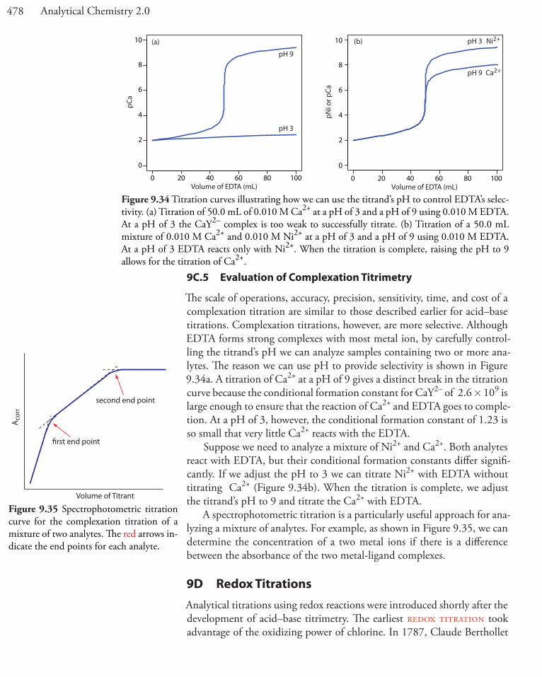
478 Analytical Chemistry 2.0
9C.5 Evaluation of Complexation Titrimetry
The scale of operations, accuracy, precision, sensitivity, time, and cost of a complexation titration are similar to those described earlier for acid–base titrations. Complexation titrations, however, are more selective. Although EDTA forms strong complexes with most metal ion, by carefully control-ling the titrand’s pH we can analyze samples containing two or more ana-lytes. The reason we can use pH to provide selectivity is shown in Figure 9.34a. A titration of Ca2+ at a pH of 9 gives a distinct break in the titration curve because the conditional formation constant for CaY2– of 2.6 � 109 is large enough to ensure that the reaction of Ca2+ and EDTA goes to comple-tion. At a pH of 3, however, the conditional formation constant of 1.23 is so small that very little Ca2+ reacts with the EDTA.
Suppose we need to analyze a mixture of Ni2+ and Ca2+. Both analytes react with EDTA, but their conditional formation constants differ signifi-cantly. If we adjust the pH to 3 we can titrate Ni2+ with EDTA without titrating Ca2+ (Figure 9.34b). When the titration is complete, we adjust the titrand’s pH to 9 and titrate the Ca2+ with EDTA.
A spectrophotometric titration is a particularly useful approach for ana-lyzing a mixture of analytes. For example, as shown in Figure 9.35, we can determine the concentration of a two metal ions if there is a difference between the absorbance of the two metal-ligand complexes.
9D Redox TitrationsAnalytical titrations using redox reactions were introduced shortly after the development of acid–base titrimetry. The earliest redox titration took advantage of the oxidizing power of chlorine. In 1787, Claude Berthollet
Figure 9.34 Titration curves illustrating how we can use the titrand’s pH to control EDTA’s selec-tivity. (a) Titration of 50.0 mL of 0.010 M Ca2+ at a pH of 3 and a pH of 9 using 0.010 M EDTA. At a pH of 3 the CaY2– complex is too weak to successfully titrate. (b) Titration of a 50.0 mL mixture of 0.010 M Ca2+ and 0.010 M Ni2+ at a pH of 3 and a pH of 9 using 0.010 M EDTA. At a pH of 3 EDTA reacts only with Ni2+. When the titration is complete, raising the pH to 9 allows for the titration of Ca2+.
Figure 9.35 Spectrophotometric titration curve for the complexation titration of a mixture of two analytes. The red arrows in-dicate the end points for each analyte.
0 20 40 60 80 100
0
2
4
6
8
10
Volume of EDTA (mL)
pCa
(a)
pH 3
pH 9
0 20 40 60 80 100
0
2
4
6
8
10
Volume of EDTA (mL)
pNi o
r pCa
(b) pH 3 Ni2+
pH 9 Ca2+
Aco
rr
Volume of Titrant
�rst end point
second end point
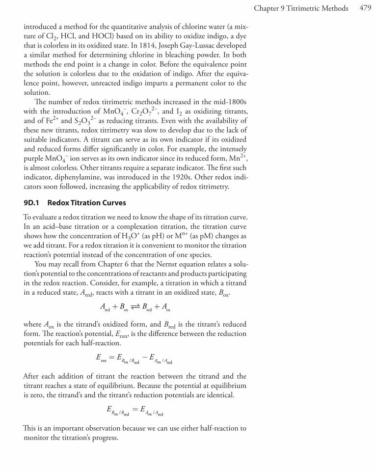
479Chapter 9 Titrimetric Methods
introduced a method for the quantitative analysis of chlorine water (a mix-ture of Cl2, HCl, and HOCl) based on its ability to oxidize indigo, a dye that is colorless in its oxidized state. In 1814, Joseph Gay-Lussac developed a similar method for determining chlorine in bleaching powder. In both methods the end point is a change in color. Before the equivalence point the solution is colorless due to the oxidation of indigo. After the equiva-lence point, however, unreacted indigo imparts a permanent color to the solution.
The number of redox titrimetric methods increased in the mid-1800s with the introduction of MnO4
–, Cr2O72–, and I2 as oxidizing titrants,
and of Fe2+ and S2O32– as reducing titrants. Even with the availability of
these new titrants, redox titrimetry was slow to develop due to the lack of suitable indicators. A titrant can serve as its own indicator if its oxidized and reduced forms differ significantly in color. For example, the intensely purple MnO4
– ion serves as its own indicator since its reduced form, Mn2+, is almost colorless. Other titrants require a separate indicator. The first such indicator, diphenylamine, was introduced in the 1920s. Other redox indi-cators soon followed, increasing the applicability of redox titrimetry.
9D.1 Redox Titration Curves
To evaluate a redox titration we need to know the shape of its titration curve. In an acid–base titration or a complexation titration, the titration curve shows how the concentration of H3O+ (as pH) or Mn+ (as pM) changes as we add titrant. For a redox titration it is convenient to monitor the titration reaction’s potential instead of the concentration of one species.
You may recall from Chapter 6 that the Nernst equation relates a solu-tion’s potential to the concentrations of reactants and products participating in the redox reaction. Consider, for example, a titration in which a titrand in a reduced state, Ared, reacts with a titrant in an oxidized state, Box.
A B B Ared ox red ox+ +
where Aox is the titrand’s oxidized form, and Bred is the titrant’s reduced form. The reaction’s potential, Erxn, is the difference between the reduction potentials for each half-reaction.
E E EB B A Arxn ox red ox red= −/ /
After each addition of titrant the reaction between the titrand and the titrant reaches a state of equilibrium. Because the potential at equilibrium is zero, the titrand’s and the titrant’s reduction potentials are identical.
E EB B A Aox red ox red/ /=
This is an important observation because we can use either half-reaction to monitor the titration’s progress.

480 Analytical Chemistry 2.0
Before the equivalence point the titration mixture consists of appreciable quantities of the titrand’s oxidized and reduced forms. The concentration of unreacted titrant, however, is very small. The potential, therefore, is easier to calculate if we use the Nernst equation for the titrand’s half-reaction
E ERTnF
AAA Arxn
o red
oxox red
= −/ ln[ ][ ]
After the equivalence point it is easier to calculate the potential using the Nernst equation for the titrant’s half-reaction.
E ERTnF
BBB Brxn
o red
oxox red
= −/ ln[ ][ ]
calculaTing The TiTraTion curve
Let’s calculate the titration curve for the titration of 50.0 mL of 0.100 M Fe2+ with 0.100 M Ce4+ in a matrix of 1 M HClO4. The reaction in this case is
Fe Ce Ce Fe2 4 3 3+ + + ++ +( ) ( ) ( ) ( )aq aq aq aq 9.15
Because the equilibrium constant for reaction 9.15 is very large—it is ap-proximately 6 � 1015—we may assume that the analyte and titrant react completely.
The first task is to calculate the volume of Ce4+ needed to reach the titra-tion’s equivalence point. From the reaction’s stoichiometry we know that
moles Fe moles Ce2+ += 4
M V M VFe Fe Ce Ce� = �
Solving for the volume of Ce4+ gives the equivalence point volume as
V VM V
Meq CeFe Fe
Ce
M)(50.0 mL)(0.100
= = =( .0 100
MM)50.0 mL=
Before the equivalence point, the concentration of unreacted Fe2+ and the concentration of Fe3+ are easy to calculate. For this reason we find the potential using the Nernst equation for the Fe3+/Fe2+ half-reaction.
E ERTnF
= − =
+ −
+ +
+
+Fe Feo Fe
Fe
V
3 2
2
3
0 767 0
/log
[ ][ ]
. .. log[ ][ ]
059162
3
FeFe
+
+
9.16
For example, the concentrations of Fe2+ and Fe3+ after adding 10.0 mL of titrant are
Although the Nernst equation is written in terms of the half-reaction’s standard state potential, a matrix-dependent for-mal potential often is used in its place. See Appendix 13 for the standard state po-tentials and formal potentials for selected half-reactions.
In 1 M HClO4, the formal potential for the reduction of Fe3+ to Fe2+ is +0.767 V, and the formal potential for the reduction of Ce4+ to Ce3+ is +1.70 V.
Step 1: Calculate the volume of titrant
needed to reach the equivalence point.
Step 2: Calculate the potential before the equivalence point by determining the concentrations of the titrand’s oxidized and reduced forms, and using the Nernst equation for the titrand’s reduction half-reaction.

481Chapter 9 Titrimetric Methods
[ ]Feinitial moles Fe moles Ce added
t2
2 4+
+ +
=−
ootal volumeM)
Fe Fe Ce Ce
Fe Ce
=−+
=
M V M VV V
( .0 100 ((50.0 mL) M)(10.0 mL)50.0 mL .0 m
−+
( .0 10010 LL
M= � −6 67 10 2.
[ ]Femoles Ce added
total volumeCe Ce3
4+
+
= =M V
VFFe Ce
M)(10.0 mL)50.0 mL .0 mL
+
=+
=
V
( .0 10010
1..67 10 2� − M
Substituting these concentrations into equation 9.16 gives a potential of
E =+ −��
−
−0 767 0 05916
6 67 101 67 10
2
2. . log
.
.V
MM=+0 731. V
After the equivalence point, the concentration of Ce3+ and the con-centration of excess Ce4+ are easy to calculate. For this reason we find the potential using the Nernst equation for the Ce4+/Ce3+ half-reaction.
E ERTnFCe C
= − =
+ −
+ +
+
+4 3
3
4
1 70 0
/log
[ ][ ]
.
eo Ce
Ce
V .. log[ ][ ]
059163
4
CeCe
+
+
9.17
For example, after adding 60.0 mL of titrant, the concentrations of Ce3+ and Ce4+ are
[ ]Ceinitial moles Fe
total volumeFe F3
2+
+
= =M V ee
Fe Ce
M)(50.0 mL)50.0 mL 0 mL
V V+
=+
( ..
0 10060
== � −4 55 10 3. M
[ ]Cemoles Ce added initial moles Fe
t4
4 2+
+ +
=−
ootal volumeM)
Ce Ce Fe Fe
Fe Ce
=−+
=
M V M VV V
( .0 100 ((60.0 mL) M)(50.0 mL)50.0 mL 60.0 m
−+
( .0 100LL
M= � −9 09 10 3.
Substituting these concentrations into equation 9.17 gives a potential of
E =+ −��
−
−1 70 0 05916
4 55 109 09 10
2
3. . log
.
.V
MM=+1 66. V
At the titration’s equivalence point, the potential, Eeq, in equation 9.16 and equation 9.17 are identical. Adding the equations together to gives
Step 3: Calculate the potential after the equivalence point by determining the concentrations of the titrant’s oxidized and reduced forms, and using the Nernst equation for the titrant’s reduction half-reaction.
Step 4: Calculate the potential at the equivalence point.
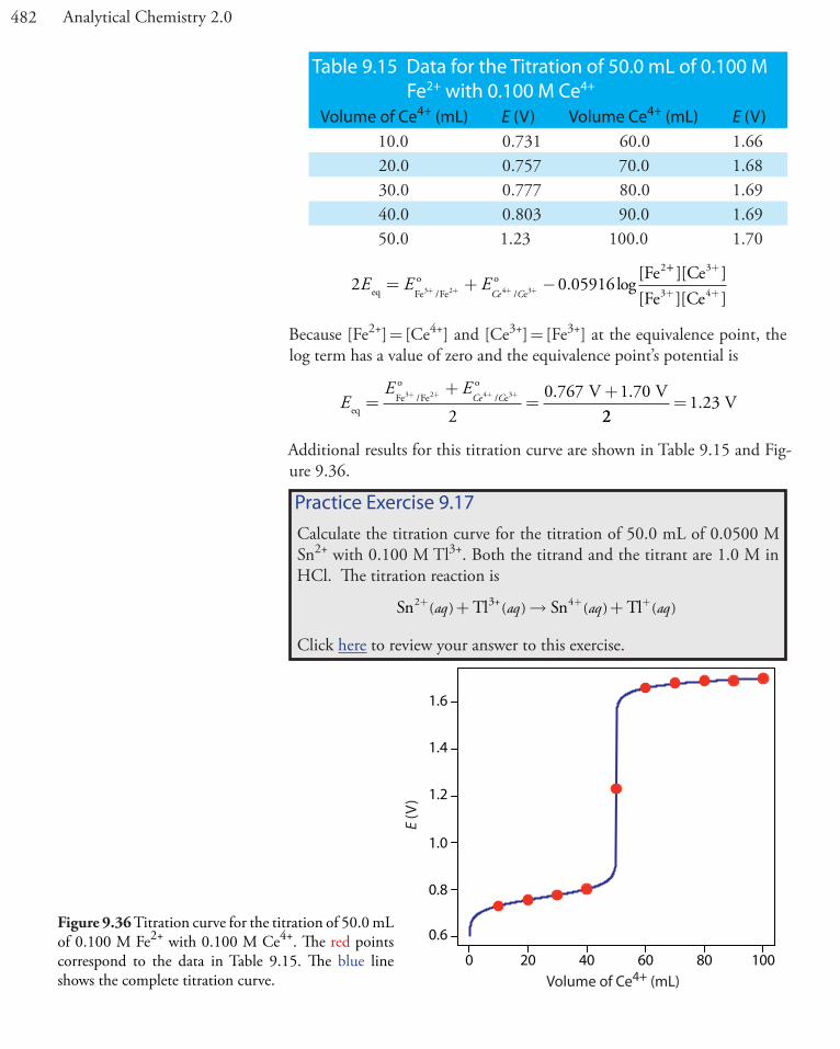
482 Analytical Chemistry 2.0
2 0 059163 2 4 3
2
E E ECe Ceq Fe Fe
oe
o Fe= + −+ + + +/ /
. log[ ++ +
+ +
][ ][ ][ ]
CeFe Ce
3
3 4
Because [Fe2+] = [Ce4+] and [Ce3+] = [Fe3+] at the equivalence point, the log term has a value of zero and the equivalence point’s potential is
EE E
Ce Ceq
Fe Feo
eo V V
=+
=++ + + +3 2 4 3
20 767 1 70/ / . .
221 23= . V
Additional results for this titration curve are shown in Table 9.15 and Fig-ure 9.36.
Practice Exercise 9.17Calculate the titration curve for the titration of 50.0 mL of 0.0500 M Sn2+ with 0.100 M Tl3+. Both the titrand and the titrant are 1.0 M in HCl. The titration reaction is
Sn Tl Sn Tl3+2 4+ + ++ → +( ) ( ) ( ) ( )aq aq aq aq
Click here to review your answer to this exercise.
Table 9.15 Data for the Titration of 50.0 mL of 0.100 M Fe2+ with 0.100 M Ce4+
Volume of Ce4+ (mL) E (V) Volume Ce4+ (mL) E (V)10.0 0.731 60.0 1.6620.0 0.757 70.0 1.6830.0 0.777 80.0 1.6940.0 0.803 90.0 1.6950.0 1.23 100.0 1.70
Figure 9.36 Titration curve for the titration of 50.0 mL of 0.100 M Fe2+ with 0.100 M Ce4+. The red points correspond to the data in Table 9.15. The blue line shows the complete titration curve.
0 20 40 60 80 100
0.6
0.8
1.0
1.2
1.4
1.6
Volume of Ce4+ (mL)
E (V
)
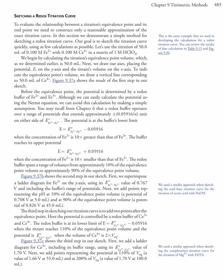
483Chapter 9 Titrimetric Methods
This is the same example that we used in developing the calculations for a redox titration curve. You can review the results of that calculation in Table 9.15 and Fig-ure 9.36.
We used a similar approach when sketch-ing the complexation titration curve for the titration of Mg2+ with EDTA.
SkeTching a redox TiTraTion curve
To evaluate the relationship between a titration’s equivalence point and its end point we need to construct only a reasonable approximation of the exact titration curve. In this section we demonstrate a simple method for sketching a redox titration curve. Our goal is to sketch the titration curve quickly, using as few calculations as possible. Let’s use the titration of 50.0 mL of 0.100 M Fe2+ with 0.100 M Ce4+ in a matrix of 1 M HClO4.
We begin by calculating the titration’s equivalence point volume, which, as we determined earlier, is 50.0 mL. Next, we draw our axes, placing the potential, E, on the y-axis and the titrant’s volume on the x-axis. To indi-cate the equivalence point’s volume, we draw a vertical line corresponding to 50.0 mL of Ce4+. Figure 9.37a shows the result of the first step in our sketch.
Before the equivalence point, the potential is determined by a redox buffer of Fe2+ and Fe3+. Although we can easily calculate the potential us-ing the Nernst equation, we can avoid this calculation by making a simple assumption. You may recall from Chapter 6 that a redox buffer operates over a range of potentials that extends approximately ±(0.05916/n) unit on either side of E
Fe Feo
3 2+ +/. The potential is at the buffer’s lower limit
E = EFe Feo
3 2+ +/ – 0.05916
when the concentration of Fe2+ is 10� greater than that of Fe3+. The buffer reaches its upper potential
E = EFe Feo
3 2+ +/ + 0.05916
when the concentration of Fe2+ is 10� smaller than that of Fe3+. The redox buffer spans a range of volumes from approximately 10% of the equivalence point volume to approximately 90% of the equivalence point volume.
Figure 9.37b shows the second step in our sketch. First, we superimpose a ladder diagram for Fe2+ on the y-axis, using its E
Fe Feo
3 2+ +/ value of 0.767 V and including the buffer’s range of potentials. Next, we add points rep-resenting the pH at 10% of the equivalence point volume (a potential of 0.708 V at 5.0 mL) and at 90% of the equivalence point volume (a poten-tial of 0.826 V at 45.0 mL).
The third step in sketching our titration curve is to add two points after the equivalence point. Here the potential is controlled by a redox buffer of Ce3+ and Ce4+. The redox buffer is at its lower limit of E = ECe Ce
o4 3+ +/ – 0.05916
when the titrant reaches 110% of the equivalence point volume and the potential is E
Ce Ceo
4 3+ +/ when the volume of Ce4+ is 2�Veq.
Figure 9.37c shows the third step in our sketch. First, we add a ladder diagram for Ce4+, including its buffer range, using its E
Ce Ceo
4 3+ +/ value of
1.70 V. Next, we add points representing the potential at 110% of Veq (a value of 1.66 V at 55.0 mL) and at 200% of Veq (a value of 1.70 V at 100.0 mL).
We used a similar approach when sketch-ing the acid–base titration curve for the titration of acetic acid with NaOH.
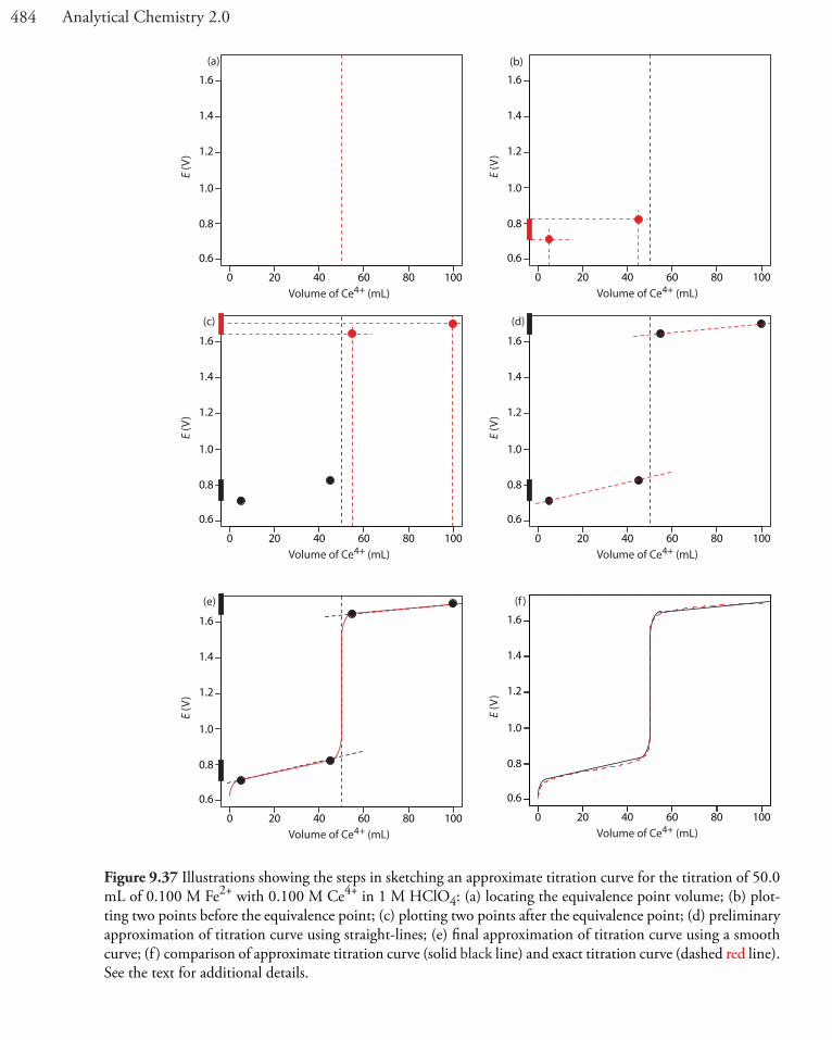
484 Analytical Chemistry 2.0
Figure 9.37 Illustrations showing the steps in sketching an approximate titration curve for the titration of 50.0 mL of 0.100 M Fe2+ with 0.100 M Ce4+ in 1 M HClO4: (a) locating the equivalence point volume; (b) plot-ting two points before the equivalence point; (c) plotting two points after the equivalence point; (d) preliminary approximation of titration curve using straight-lines; (e) final approximation of titration curve using a smooth curve; (f ) comparison of approximate titration curve (solid black line) and exact titration curve (dashed red line). See the text for additional details.
0 20 40 60 80 100
0.6
0.8
1.0
1.2
1.4
1.6
Volume of Ce4+ (mL)
E (V
)
(a)
0 20 40 60 80 100
0.6
0.8
1.0
1.2
1.4
1.6
Volume of Ce4+ (mL)
E (V
)
(b)
0 20 40 60 80 100
0.6
0.8
1.0
1.2
1.4
1.6
Volume of Ce4+ (mL)
E (V
)
(c)
0 20 40 60 80 100
0.6
0.8
1.0
1.2
1.4
1.6
Volume of Ce4+ (mL)
E (V
)
(d)
0 20 40 60 80 100
0.6
0.8
1.0
1.2
1.4
1.6
Volume of Ce4+ (mL)
E (V
)
(e)
0 20 40 60 80 100
0.6
0.8
1.0
1.2
1.4
1.6
Volume of Ce4+ (mL)
E (V
)
(f )

485Chapter 9 Titrimetric Methods
Next, we draw a straight line through each pair of points, extending the line through the vertical line representing the equivalence point’s volume (Figure 9.37d). Finally, we complete our sketch by drawing a smooth curve that connects the three straight-line segments (Figure 9.37e). A comparison of our sketch to the exact titration curve (Figure 9.37f ) shows that they are in close agreement.Practice Exercise 9.18Sketch the titration curve for the titration of 50.0 mL of 0.0500 M Sn4+ with 0.100 M Tl+. Both the titrand and the titrant are 1.0 M in HCl. The titration reaction is
Sn Tl Sn Tl3+2 4+ + ++ → +( ) ( ) ( ) ( )aq aq aq aq
Compare your sketch to your calculated titration curve from Practice Exercise 9.17.
Click here to review your answer to this exercise.
We often use H+ instead of H3O+ when writing a redox reaction.
9D.2 Selecting and Evaluating the End point
A redox titration’s equivalence point occurs when we react stoichiometrical-ly equivalent amounts of titrand and titrant. As is the case with acid–base and complexation titrations, we estimate the equivalence point of a com-plexation titration using an experimental end point. A variety of methods are available for locating the end point, including indicators and sensors that respond to a change in the solution conditions.
Where iS The equivalence PoinT?
For an acid–base titration or a complexometric titration the equivalence point is almost identical to the inflection point on the steeping rising part of the titration curve. If you look back at Figure 9.7 and Figure 9.28, you will see that the inflection point is in the middle of this steep rise in the titration curve, which makes it relatively easy to find the equivalence point when you sketch these titration curves. We call this a symmetric equivalence point. If the stoichiometry of a redox titration is symmetric—one mole of titrant reacts with each mole of titrand—then the equivalence point is symmetric. If the titration reaction’s stoichiometry is not 1:1, then the equivalence point is closer to the top or to bottom of the titration curve’s sharp rise. In this case we have an asymmetric equivalence point.
Example 9.10
Derive a general equation for the equivalence point’s potential when titrat-ing Fe2+ with MnO4
–.
5 8 524
3 2Fe MnO H Fe Mn+ − + + ++ + → +( ) ( ) ( ) ( ) (aq aq aq aq aaq )+ 4H O2
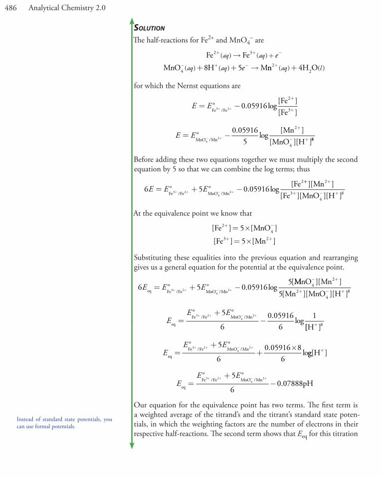
486 Analytical Chemistry 2.0
Solution
The half-reactions for Fe2+ and MnO4– are
Fe FeMnO H M
2 3
4 8 5
+ + −
− + −
→
+ + →
+( ) ( )
( ) ( )
aq aq
aq aq
e
e nn H O22 4+ +( ) ( )aq l
for which the Nernst equations are
E E= −+ +
+
+Fe Feo Fe
Fe3 2 0 05916
2
3/. log
[ ][ ]
E E= −− +
+
− +MnO Mno
4
MnMnO H/
.log
[ ][ ][ ]
2
0 059165
2
488
Before adding these two equations together we must multiply the second equation by 5 so that we can combine the log terms; thus
6 5 0 059163 2 2
2
E E E= + −+ + − +Fe Feo
MnO Mno
4
Fe/ /
. log[ ++ +
+ − +
][ ][ ][ ][ ]
MnFe MnO H
2
34
8
At the equivalence point we know that
[ ] [ ]
[ ] [ ]
Fe MnO
Fe Mn
24
3 2
5
5
+ −
+ +
= �
= �
Substituting these equalities into the previous equation and rearranging gives us a general equation for the potential at the equivalence point.
6 5 0 059165
3 2 2E E Eeq Fe Feo
MnO Mno
4= + −+ + − +/ /
. log[MMnO Mn
Mn MnO H4
2
24
85
− +
+ − +
][ ][ ][ ][ ]
EE E
eqFe Feo
MnO Mno
4=+
−+ + − +3 2 25
60 05916
61/ / .
log[[ ]H+ 8
EE E
eqFe Feo
MnO Mno
4=+
+�+ + − +3 2 25
60 05916 8
6/ / .
logg[ ]H+
EE E
eqFe Feo
MnO Mno
4 pH=+
−+ + − +3 2 25
60 07888/ / .
Our equation for the equivalence point has two terms. The first term is a weighted average of the titrand’s and the titrant’s standard state poten-tials, in which the weighting factors are the number of electrons in their respective half-reactions. The second term shows that Eeq for this titration
Instead of standard state potentials, you can use formal potentials.

487Chapter 9 Titrimetric Methods
is pH-dependent. At a pH of 1 (in H2SO4), for example, the equivalence point has a potential of
Eeq V=+ �
− � =0 768 5 1 51
60 07888 1 1 31
. .. .
Figure 9.38 shows a typical titration curve for titration of Fe2+ with MnO4–.
Note that the titration’s equivalence point is asymmetrical.
Practice Exercise 9.19Derive a general equation for the equivalence point’s potential for the titration of U4+ with Ce4+. The unbalanced reaction is
Ce U UO Ce4 422 3+ + + ++ → +( ) ( ) ( ) ( )aq aq aq aq
What is the equivalence point’s potential if the pH is 1?
Click here to review your answer to this exercise.
Figure 9.38 Titration curve for the titration of 50.0 mL of 0.100 M Fe2+ with 0.0200 M MnO4
– at a fixed pH of 1 (using H2SO4). The equivalence point is shown by the red dot.
Finding The end PoinT WiTh an indicaTor
Three types of indicators are used to signal a redox titration’s end point. The oxidized and reduced forms of some titrants, such as MnO4
–, have differ-ent colors. A solution of MnO4
– is intensely purple. In an acidic solution, however, permanganate’s reduced form, Mn2+, is nearly colorless. When using MnO4
– as a titrant, the titrand’s solution remains colorless until the equivalence point. The first drop of excess MnO4
– produces a permanent tinge of purple, signaling the end point.
Some indicators form a colored compound with a specific oxidized or reduced form of the titrant or the titrand. Starch, for example, forms a dark blue complex with I3
–. We can use this distinct color to signal the presence of excess I3
– as a titrant—a change in color from colorless to blue—or the
0 20 40 60 80 100
0.4
0.6
0.8
1.0
1.2
1.4
Volume of MnO4– (mL)
E (V
)
equivalence point

488 Analytical Chemistry 2.0
completion of a reaction consuming I3– as the titrand—a change in color
from blue to colorless. Another example of a specific indicator is thiocya-nate, SCN–, which forms a soluble red-colored complex of Fe(SCN)2+ with Fe3+.
The most important class of indicators are substances that do not par-ticipate in the redox titration, but whose oxidized and reduced forms differ in color. When we add a redox indicator to the titrand, the indicator imparts a color that depends on the solution’s potential. As the solution’s potential changes with the addition of titrant, the indicator changes oxida-tion state and changes color, signaling the end point.
To understand the relationship between potential and an indicator’s color, consider its reduction half-reaction
In Inox red+ −ne
where Inox and Inred are, respectively, the indicator’s oxidized and reduced forms. The Nernst equation for this half-reaction is
E En
= −In /Ino red
oxox red
[In ][In ]
0 05916.log
As shown in Figure 9.39, if we assume that the indicator’s color changes from that of Inox to that of Inred when the ratio [Inred]/[Inox] changes from 0.1 to 10, then the end point occurs when the solution’s potential is within the range
E En
= ±In /Ino
ox red
0 05916.
For simplicity, Inox and Inred are shown without specific charges. Because there is a change in oxidation state, Inox and Inred cannot both be neutral.
This is the same approach we took in con-sidering acid–base indicators and compl-exation indicators.
Figure 9.39 Diagram showing the relationship between E and an indicator’s color. The ladder diagram defines poten-tials where Inred and Inox are the predominate species. The indicator changes color when E is within the range
E En
= ±In /Ino
ox red
0 05916.
Inox
Inred
E = EInox/Inredindicator’s
color transitionrange
indicatoris color of Inox
indicatoris color of Inred
E
o

489Chapter 9 Titrimetric Methods
Table 9.16 Selected Examples of Redox Indicators
Indicator Color of Inox Color of InredEIn / In
o
ox red
indigo tetrasulfate blue colorless 0.36methylene blue blue colorless 0.53diphenylamine violet colorless 0.75diphenylamine sulfonic acid red-violet colorless 0.85tris(2,2´-bipyridine)iron pale blue red 1.120ferroin pale blue red 1.147tris(5-nitro-1,10-phenanthroline)iron pale blue red-violet 1.25
Figure 9.40 Titration curve for the titration of 50.0 mL of 0.100 M Fe2+ with 0.100 M Ce4+. The end point transitions for the indicators diphenylamine sulfonic acid and ferroin are superimposed on the titration curve. Because the transition for ferroin is too small to see on the scale of the x-axis—it re-quires only 1–2 drops of titrant—the color change is expanded to the right.
A partial list of redox indicators is shown in Table 9.16. Examples of ap-propriate and inappropriate indicators for the titration of Fe2+ with Ce4+ are shown in Figure 9.40.
oTher MeThodS For Finding The end PoinT
Another method for locating a redox titration’s end point is a potentio-metric titration in which we monitor the change in potential while adding the titrant to the titrand. The end point is found by visually examining the titration curve. The simplest experimental design for a potentiometric titration consists of a Pt indicator electrode whose potential is governed by the titrand’s or titrant’s redox half-reaction, and a reference electrode that has a fixed potential. A further discussion of potentiometry is found in Chapter 11. Other methods for locating the titration’s end point include thermometric titrations and spectrophotometric titrations.
0 20 40 60 80 100
0.6
0.8
1.0
1.2
1.4
1.6
Volume of Ce4+ (mL)
E (V
)
diphenylaminesulfonic acid
ferroin
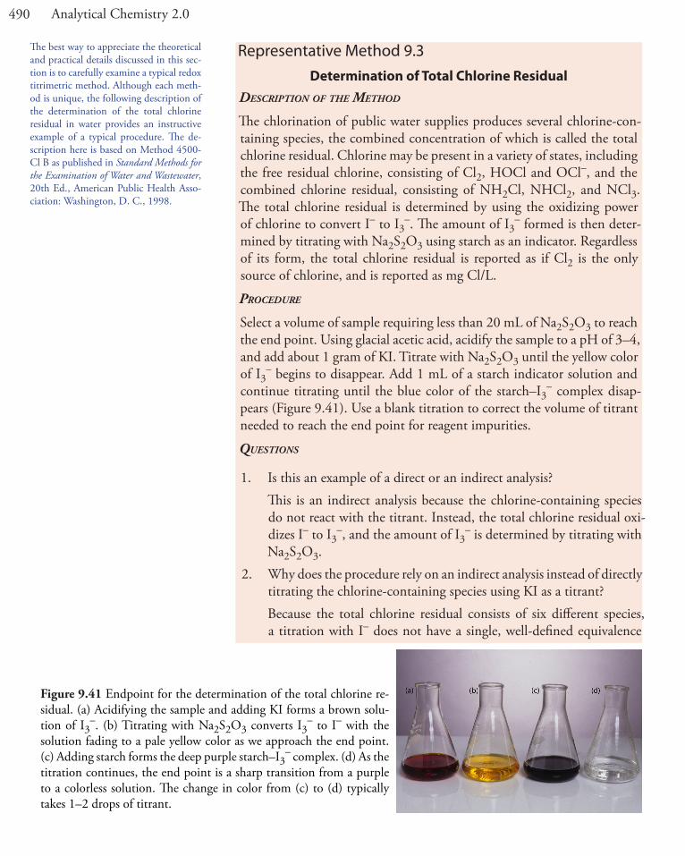
490 Analytical Chemistry 2.0
Representative Method 9.3 Determination of Total Chlorine Residual
Description of the MethoD
The chlorination of public water supplies produces several chlorine-con-taining species, the combined concentration of which is called the total chlorine residual. Chlorine may be present in a variety of states, including the free residual chlorine, consisting of Cl2, HOCl and OCl–, and the combined chlorine residual, consisting of NH2Cl, NHCl2, and NCl3. The total chlorine residual is determined by using the oxidizing power of chlorine to convert I– to I3
–. The amount of I3– formed is then deter-
mined by titrating with Na2S2O3 using starch as an indicator. Regardless of its form, the total chlorine residual is reported as if Cl2 is the only source of chlorine, and is reported as mg Cl/L.
proceDure
Select a volume of sample requiring less than 20 mL of Na2S2O3 to reach the end point. Using glacial acetic acid, acidify the sample to a pH of 3–4, and add about 1 gram of KI. Titrate with Na2S2O3 until the yellow color of I3
– begins to disappear. Add 1 mL of a starch indicator solution and continue titrating until the blue color of the starch–I3
– complex disap-pears (Figure 9.41). Use a blank titration to correct the volume of titrant needed to reach the end point for reagent impurities.
Questions
1. Is this an example of a direct or an indirect analysis? This is an indirect analysis because the chlorine-containing species
do not react with the titrant. Instead, the total chlorine residual oxi-dizes I– to I3
–, and the amount of I3– is determined by titrating with
Na2S2O3.2. Why does the procedure rely on an indirect analysis instead of directly
titrating the chlorine-containing species using KI as a titrant? Because the total chlorine residual consists of six different species,
a titration with I– does not have a single, well-defined equivalence
The best way to appreciate the theoretical and practical details discussed in this sec-tion is to carefully examine a typical redox titrimetric method. Although each meth-od is unique, the following description of the determination of the total chlorine residual in water provides an instructive example of a typical procedure. The de-scription here is based on Method 4500-Cl B as published in Standard Methods for the Examination of Water and Wastewater, 20th Ed., American Public Health Asso-ciation: Washington, D. C., 1998.
Figure 9.41 Endpoint for the determination of the total chlorine re-sidual. (a) Acidifying the sample and adding KI forms a brown solu-tion of I3
–. (b) Titrating with Na2S2O3 converts I3– to I– with the
solution fading to a pale yellow color as we approach the end point. (c) Adding starch forms the deep purple starch–I3
– complex. (d) As the titration continues, the end point is a sharp transition from a purple to a colorless solution. The change in color from (c) to (d) typically takes 1–2 drops of titrant.

491Chapter 9 Titrimetric Methods
9D.3 Quantitative Applications
Although many quantitative applications of redox titrimetry have been re-placed by other analytical methods, a few important applications continue to be relevant. In this section we review the general application of redox titrimetry with an emphasis on environmental, pharmaceutical, and indus-trial applications. We begin, however, with a brief discussion of selecting and characterizing redox titrants, and methods for controlling the titrand’s oxidation state.
adjuSTing The TiTrand’S oxidaTion STaTe
If a redox titration is to be used in a quantitative analysis, the titrand must initially be present in a single oxidation state. For example, iron can be de-termined by a redox titration in which Ce4+ oxidizes Fe2+ to Fe3+. Depend-ing on the sample and the method of sample preparation, iron may initially be present in both the +2 and +3 oxidation states. Before titrating, we must reduce any Fe3+ to Fe2+. This type of pretreatment can be accomplished using an auxiliary reducing agent or oxidizing agent.
A metal that is easy to oxidize—such as Zn, Al, and Ag—can serve as an auxiliary reducinG aGent. The metal, as a coiled wire or powder, is added to the sample where it reduces the titrand. Because any unreacted auxiliary reducing agent will react with the titrant, it must be removed be-fore beginning the titration. This can be accomplished by simply removing the coiled wire, or by filtering.
An alternative method for using an auxiliary reducing agent is to im-mobilize it in a column. To prepare a reduction column an aqueous slurry
point. By converting the chlorine residual to an equivalent amount of I3
–, the indirect titration with Na2S2O3 has a single, useful equiva-lence point.
Even if the total chlorine residual is from a single species, such as HOCl, a direct titration with KI is impractical. Because the product of the titration, I3
–, imparts a yellow color, the titrand’s color would change with each addition of titrant, making it difficult to find a suit-able indicator.
3. Both oxidizing and reducing agents can interfere with this analysis. Explain the effect of each type of interferent has on the total chlorine residual.
An interferent that is an oxidizing agent converts additional I– to I3–.
Because this extra I3– requires an additional volume of Na2S2O3 to
reach the end point, we overestimate the total chlorine residual. If the interferent is a reducing agent, it reduces back to I– some of the I3
– produced by the reaction between the total chlorine residual and iodide. As a result. we underestimate the total chlorine residual.

492 Analytical Chemistry 2.0
of the finally divided metal is packed in a glass tube equipped with a porous plug at the bottom. The sample is placed at the top of the column and moves through the column under the influence of gravity or vacuum suc-tion. The length of the reduction column and the flow rate are selected to ensure the analyte’s complete reduction.
Two common reduction columns are used. In the jones reductor the column is filled with amalgamated zinc, Zn(Hg), prepared by briefly plac-ing Zn granules in a solution of HgCl2. Oxidation of zinc
Zn(Hg) Zn Hg( ) ( ) ( )s aq l e→ + ++ −2 2
provides the electrons for reducing the titrand. In the Walden reductor the column is filled with granular Ag metal. The solution containing the titrand is acidified with HCl and passed through the column where the oxidation of silver
Ag Cl AgCl( ) ( ) ( )s aq s e+ → +− −
provides the necessary electrons for reducing the titrand. Table 9.17 pro-vides a summary of several applications of reduction columns.
Several reagents are commonly used as auxiliary oxidizinG aGents, including ammonium peroxydisulfate, (NH4)2S2O8, and hydrogen perox-ide, H2O2. Peroxydisulfate is a powerful oxidizing agent
S O SO2 82
422 2− − −+ →( ) ( )aq aqe
Table 9.17 Examples of Reactions For Reducing a Titrand’s Oxidation State Using a Reduction Column
Oxidized Titrand Walden Reductor Jones Reductor
Cr3+ — Cr Cr3 2+ − ++ →( ) ( )aq aqe
Cu2+ Cu Cu2+ − ++ →( ) ( )aq aqe Cu Cr2 2+ −+ →( ) ( )aq se
Fe3+ Fe Fe3 2+ − ++ →( ) ( )aq aqe Fe Fe3 2+ − ++ →( ) ( )aq aqe
TiO2+ —TiO H
Ti H O2
2
3
2+ + −
+
+ +
→ +
( ) ( )
( ) ( )
aq aq
aq l
e
MoO22+ MoO MoO2
22
+ − ++ →( ) ( )aq aqeMoO H
Mo H O22+
2
( ) ( )
( ) ( )
aq aq
aq l
e+ +
→ +
+ −
+
4 3
23
VO2+
VO H
VO H O22
2 2+ + −
+
+ +
→ +
( ) ( )
( ) ( )
aq aq
aq l
e VO H
V H O2+
2
( ) ( )
( ) ( )
aq aq
aq l
e+ +
→ +
+ −
+
4 3
22

493Chapter 9 Titrimetric Methods
capable of oxidizing Mn2+ to MnO4–, Cr3+ to Cr2O7
2–, and Ce3+ to Ce4+. Excess peroxydisulfate is easily destroyed by briefly boiling the solution. The reduction of hydrogen peroxide in acidic solution
H O H H O2 2 2( ) ( ) ( )aq aq le+ + →+ −2 2 2
provides another method for oxidizing a titrand. Excess H2O2 is destroyed by briefly boiling the solution.
SelecTing and STandardizing a TiTranT
If it is to be used quantitatively, the titrant’s concentration must remain stable during the analysis. Because a titrant in a reduced state is suscep-tible to air oxidation, most redox titrations use an oxidizing agent as the titrant. There are several common oxidizing titrants, including MnO4
–, Ce4+, Cr2O7
2–, and I3–. Which titrant is used often depends on how easy
it is to oxidize the titrand. A titrand that is a weak reducing agent needs a strong oxidizing titrant if the titration reaction is to have a suitable end point.
The two strongest oxidizing titrants are MnO4– and Ce4+, for which the
reduction half-reactions are
MnO H Mn H O2428 5 4− + − ++ + +( ) ( ) ( ) ( )aq aq aq le
Ce Ce4 3+ − ++( ) ( )aq aqe
Solutions of Ce4+ usually are prepared from the primary standard cerium ammonium nitrate, Ce(NO3)4•2NH4NO3, in 1 M H2SO4. When pre-pared using a reagent grade material, such as Ce(OH)4, the solution is standardized against a primary standard reducing agent such as Na2C2O4 or Fe2+ (prepared using iron wire) using ferroin as an indicator. Despite its availability as a primary standard and its ease of preparation, Ce4+ is not as frequently used as MnO4
– because it is more expensive.Solutions of MnO4
– are prepared from KMnO4, which is not available as a primary standard. Aqueous solutions of permanganate are thermody-namically unstable due to its ability to oxidize water.
4MnO H O MnO O OH24 2 22 4 3 4− −+ + +( ) ( ) ( ) ( ) ( )aq l s g aq
This reaction is catalyzed by the presence of MnO2, Mn2+, heat, light, and the presence of acids and bases. A moderately stable solution of permangan-ate can be prepared by boiling it for an hour and filtering through a sintered glass filter to remove any solid MnO2 that precipitates. Standardization is accomplished against a primary standard reducing agent such as Na2C2O4 or Fe2+ (prepared using iron wire), with the pink color of excess MnO4
– signaling the end point. A solution of MnO4
– prepared in this fashion is stable for 1–2 weeks, although the standardization should be rechecked periodically.
The standardization reactions are
Ce Fe
Ce Fe
Ce
4 2
3 3
42
+ +
+ +
+
+ →
+
( ) ( )
( ) ( )
(
aq aq
aq aq
aq )) ( )
( ) ( ) ( )
+ →
+ ++ +
H C O
Ce CO H
2 2 4 aq
aq g aq2 2 232
The standardization reactions are
MnO Fe H4 5 82− + ++ + →( ) ( ) ( )aq aq aq
Mn Fe H O
2MnO
22 35 4
54
+ +
−
+ +
+
( ) ( ) ( )
( )
aq aq l
aq HH C O H
Mn
2 2 4 ( ) ( )
(
aq aq
a
+ →+
+
6
2 2qq g l) ( ) ( )+ +10 82CO H O2

494 Analytical Chemistry 2.0
Potassium dichromate is a relatively strong oxidizing agent whose prin-cipal advantages are its availability as a primary standard and the long term stability of its solutions. It is not, however, as strong an oxidizing agent as MnO4
– or Ce4+, which makes it less useful when the titrand is a weak reducing agent. Its reduction half-reaction is
Cr O H Cr H O2 272 314 6 2 7− + − ++ + +( ) ( ) ( ) ( )aq aq aq le
Although a solution of Cr2O72– is orange and a solution of Cr3+ is green,
neither color is intense enough to serve as a useful indicator. Diphenylam-ine sulfonic acid, whose oxidized form is red-violet and reduced form is colorless, gives a very distinct end point signal with Cr2O7
2–.Iodine is another important oxidizing titrant. Because it is a weaker
oxidizing agent than MnO4–, Ce4+, and Cr2O7
2–, it is useful only when the titrand is a stronger reducing agent. This apparent limitation, however, makes I2 a more selective titrant for the analysis of a strong reducing agent in the presence of a weaker reducing agent. The reduction half-reaction for I2 is
I I2 2 2( ) ( )aq aqe+ − −
Because iodine is not very soluble in water, solutions are prepared by adding an excess of I–. The complexation reaction
I I I2 3( ) ( ) ( )aq aq aq+ − −
increases the solubility of I2 by forming the more soluble triiodide ion, I3–.
Even though iodine is present as I3– instead of I2, the number of electrons
in the reduction half-reaction is unaffected.
I I3 2 3− − −+( ) ( )aq aqe
Solutions of I3– are normally standardized against Na2S2O3 using starch as
a specific indicator for I3–.
An oxidizing titrant such as MnO4–, Ce4+, Cr2O7
2–, and I3–, is used
when the titrand is in a reduced state. If the titrand is in an oxidized state, we can first reduce it with an auxiliary reducing agent and then complete the titration using an oxidizing titrant. Alternatively, we can titrate it using a reducing titrant. Iodide is a relatively strong reducing agent that could serve as a reducing titrant except that a solution of I– is susceptible to the air-oxidation of I– to I3
–.
3 23I I− − −+( ) ( )aq aq e
Instead, adding an excess of KI reduces the titrand, releasing a stoichiomet-ric amount of I3
–. The amount of I3– produced is then determined by a back
titration using thiosulfate, S2O32–, as a reducing titrant.
The standardization reaction is
I S O
I S O
2
4
3 32
62
2
3 2
− −
− −
+ →
+
( ) ( )
( ) ( )
aq aq
aq aq
A freshly prepared solution of KI is clear, but after a few days it may show a faint yel-low coloring due to the presence of I3
–.

495Chapter 9 Titrimetric Methods
2S O S O2 432
622 2− − −+( ) ( )aq aq e
Solutions of S2O32– are prepared using Na2S2O3•5H2O, and must be
standardized before use. Standardization is accomplished by dissolving a carefully weighed portion of the primary standard KIO3 in an acidic solu-tion containing an excess of KI. The reaction between IO3
– and I–
IO I H I H O23 38 6 3 3− − + −+ + → +( ) ( ) ( ) ( ) ( )aq aq aq aq l
liberates a stoichiometric amount of I3–. By titrating this I3
– with thiosul-fate, using starch as a visual indicator, we can determine the concentration of S2O3
2– in the titrant.Although thiosulfate is one of the few reducing titrants that is not read-
ily oxidized by contact with air, it is subject to a slow decomposition to bisulfite and elemental sulfur. If used over a period of several weeks, a solu-tion of thiosulfate should be restandardized periodically. Several forms of bacteria are able to metabolize thiosulfate, which also can lead to a change in its concentration. This problem can be minimized by adding a preserva-tive such as HgI2 to the solution.
Another useful reducing titrant is ferrous ammonium sulfate, Fe(NH4)2(SO4)2•6H2O, in which iron is present in the +2 oxidation state. A solution of Fe2+ is susceptible to air-oxidation, but when prepared in 0.5 M H2SO4 it remains stable for as long as a month. Periodic restandardiza-tion with K2Cr2O7 is advisable. The titrant can be used to directly titrate the titrand by oxidizing Fe2+ to Fe3+. Alternatively, ferrous ammonium sulfate is added to the titrand in excess and the quantity of Fe3+ produced determined by back titrating with a standard solution of Ce4+ or Cr2O7
2–.
inorganic analySiS
One of the most important applications of redox titrimetry is evaluat-ing the chlorination of public water supplies. Representative Method 9.3, for example, describes an approach for determining the total chlorine re-sidual by using the oxidizing power of chlorine to oxidize I– to I3
–. The amount of I3
– is determined by back titrating with S2O32–.
The efficiency of chlorination depends on the form of the chlorinating species. There are two contributions to the total chlorine residual—the free chlorine residual and the combined chlorine residual. The free chlorine residual includes forms of chlorine that are available for disinfecting the water supply. Examples of species contributing to the free chlorine residual include Cl2, HOCl and OCl–. The combined chlorine residual includes those species in which chlorine is in its reduced form and, therefore, no longer capable of providing disinfection. Species contributing to the com-bined chlorine residual are NH2Cl, NHCl2 and NCl3.
When a sample of iodide-free chlorinated water is mixed with an excess of the indicator N,N-diethyl-p-phenylenediamine (DPD), the free chlorine
The standardization titration is
I S O
I S O
2
4
3 32
62
2
3 2
− −
− −
+ →
+
( ) ( )
( ) ( )
aq aq
aq aq
which is the same reaction used to stan-dardize solutions of I3
–. This approach to standardizing solutions of S2O3
2– is similar to the determination of the total chlorine residual outlined in Representa-tive Method 9.3.

496 Analytical Chemistry 2.0
oxidizes a stoichiometric portion of DPD to its red-colored form. The oxidized DPD is then back titrated to its colorless form using ferrous am-monium sulfate as the titrant. The volume of titrant is proportional to the free residual chlorine.
Having determined the free chlorine residual in the water sample, a small amount of KI is added, catalyzing the reduction monochloramine, NH2Cl, and oxidizing a portion of the DPD back to its red-colored form. Titrating the oxidized DPD with ferrous ammonium sulfate yields the amount of NH2Cl in the sample. The amount of dichloramine and trichloramine are determined in a similar fashion.
The methods described above for determining the total, free, or com-bined chlorine residual also are used to establish a water supply’s chlorine demand. Chlorine demand is defined as the quantity of chlorine needed to completely react with any substance that can be oxidized by chlorine, while also maintaining the desired chlorine residual. It is determined by adding progressively greater amounts of chlorine to a set of samples drawn from the water supply and determining the total, free, or combined chlorine residual.
Another important example of redox titrimetry, which finds applica-tions in both public health and environmental analyses is the determination of dissolved oxygen. In natural waters, such as lakes and rivers, the level of dissolved O2 is important for two reasons: it is the most readily available oxidant for the biological oxidation of inorganic and organic pollutants; and it is necessary for the support of aquatic life. In a wastewater treatment plant dissolved O2 is essential for the aerobic oxidation of waste materials. If the concentration of dissolved O2 falls below a critical value, aerobic bacteria are replaced by anaerobic bacteria, and the oxidation of organic waste produces undesirable gases, such as CH4 and H2S.
One standard method for determining the dissolved O2 content of natural waters and wastewaters is the Winkler method. A sample of water is collected without exposing it to the atmosphere, which might change the concentration of dissolved O2. The sample is first treated with a solution of MnSO4, and then with a solution of NaOH and KI. Under these alkaline conditions the dissolved oxygen oxidizes Mn2+ to MnO2.
2 4 2 222 2Mn OH O MnO H O2
+ −+ + → +( ) ( ) ( ) ( ) ( )aq aq g s l
After the reaction is complete, the solution is acidified with H2SO4. Under the now acidic conditions I– is oxidized to I3
– by MnO2.
MnO I H Mn I H O222
33 4 2( ) ( ) ( ) ( ) (s aq aq aq l+ + → + +− + + − ))
The amount of I3– formed is determined by titrating with S2O3
2– using starch as an indicator. The Winkler method is subject to a variety of in-terferences, and several modifications to the original procedure have been proposed. For example, NO2
– interferes because it can reduce I3– to I– un-

497Chapter 9 Titrimetric Methods
der acidic conditions. This interference is eliminated by adding sodium azide, NaN3, reducing NO2
– to N2. Other reducing agents, such as Fe2+, are eliminated by pretreating the sample with KMnO4, and destroying the excess permanganate with K2C2O4.
Another important example of redox titrimetry is the determination of water in nonaqueous solvents. The titrant for this analysis is known as the Karl Fischer reagent and consists of a mixture of iodine, sulfur dioxide, pyri-dine, and methanol. Because the concentration of pyridine is sufficiently large, I2 and SO2 react with pyridine (py) to form the complexes py•I2 and py•SO2. When added to a sample containing water, I2 is reduced to I– and SO2 is oxidized to SO3.
py : I2 + py : SO2 + py + H2O " 2py :HI + py : SO3
Methanol is included to prevent the further reaction of py•SO3 with water. The titration’s end point is signaled when the solution changes from the product’s yellow color to the brown color of the Karl Fischer reagent.
organic analySiS
Redox titrimetry also is used for the analysis of organic analytes. One important example is the determination of the chemical oxygen demand (COD) of natural waters and wastewaters. The COD provides a measure of the quantity of oxygen necessary to completely oxidize all the organic matter in a sample to CO2 and H2O. Because no attempt is made to cor-rect for organic matter that can not be decomposed biologically, or for slow decomposition kinetics, the COD always overestimates a sample’s true oxygen demand. The determination of COD is particularly important in managing industrial wastewater treatment facilities where it is used to monitor the release of organic-rich wastes into municipal sewer systems or the environment.
A sample’s COD is determined by refluxing it in the presence of excess K2Cr2O7, which serves as the oxidizing agent. The solution is acidified with H2SO4 using Ag2SO4 to catalyze the oxidation of low molecular weight fatty acids. Mercuric sulfate, HgSO4, is added to complex any chloride that is present, preventing the precipitation of the Ag+ catalyst as AgCl. Under these conditions, the efficiency for oxidizing organic matter is 95–100%. After refluxing for two hours, the solution is cooled to room temperature and the excess Cr2O7
2– is determined by back titrating using ferrous am-monium sulfate as the titrant and ferroin as the indicator. Because it is dif-ficult to completely remove all traces of organic matter from the reagents, a blank titration must be performed. The difference in the amount of ferrous ammonium sulfate needed to titrate the sample and the blank is propor-tional to the COD.
Iodine has been used as an oxidizing titrant for a number of compounds of pharmaceutical interest. Earlier we noted that the reaction of S2O3
2–

498 Analytical Chemistry 2.0
with I3– produces the tetrathionate ion, S4O6
2–. The tetrathionate ion is actually a dimer consisting of two thiosulfate ions connected through a disulfide (–S–S–) linkage. In the same fashion, I3
– can be used to titrate mercaptans of the general formula RSH, forming the dimer RSSR as a product. The amino acid cysteine also can be titrated with I3
–. The product of this titration is cystine, which is a dimer of cysteine. Triiodide also can be used for the analysis of ascorbic acid (vitamin C) by oxidizing the enediol functional group to an alpha diketone
O
OHHO
OH
HO O
OO
OH
HOO O+ 2H+ + 2e
and for the analysis of reducing sugars, such as glucose, by oxidizing the aldehyde functional group to a carboxylate ion in a basic solution.
CHO
OHH
HHO
OHH
OHH
CH2OH
CO2
OHH
HHO
OHH
OHH
CH2OH
+ 3OH
An organic compound containing a hydroxyl, a carbonyl, or an amine functional group adjacent to an hydoxyl or a carbonyl group can be oxi-dized using metaperiodate, IO4
–, as an oxidizing titrant.
IO H O IO OH24 32 2− − − −+ + +( ) ( ) ( ) ( )aq l aq aqe
A two-electron oxidation cleaves the C–C bond between the two func-tional groups, with hydroxyl groups being oxidized to aldehydes or ke-tones, carbonyl functional groups being oxidized to carboxylic acids, and amines being oxidized to an aldehyde and an amine (ammonia if a primary amine). The analysis is conducted by adding a known excess of IO4
– to the solution containing the analyte, and allowing the oxidation to take place for approximately one hour at room temperature. When the oxidation is complete, an excess of KI is added, which converts any unreacted IO4
– to IO3
– and I3–.
IO I H O IO I O24 3 33 2− − − −+ + → + +( ) ( ) ( ) ( ) ( )aq aq l aq aq HH−( )aq
The I3– is then determined by titrating with S2O3
2– using starch as an indicator.
499Chapter 9 Titrimetric Methods
quanTiTaTive calculaTionS
The quantitative relationship between the titrand and the titrant is deter-mined by the stoichiometry of the titration reaction. If you are unsure of the balanced reaction, you can deduce the stoichiometry by remembering that the electrons in a redox reaction must be conserved.
Example 9.11
The amount of Fe in a 0.4891-g sample of an ore was determined by titrating with K2Cr2O7. After dissolving the sample in HCl, the iron was brought into the +2 oxidation state using a Jones reductor. Titration to the diphenylamine sulfonic acid end point required 36.92 mL of 0.02153 M K2Cr2O7. Report the ore’s iron content as %w/w Fe2O3.
Solution
Because we have not been provided with the titration reaction, let’s use a conservation of electrons to deduce the stoichiometry. During the titration the analyte is oxidized from Fe2+ to Fe3+, and the titrant is reduced from Cr2O7
2– to Cr3+. Oxidizing Fe2+ to Fe3+ requires only a single electron. Reducing Cr2O7
2–, in which each chromium is in the +6 oxidation state, to Cr3+ requires three electrons per chromium, for a total of six electrons. A conservation of electrons for the titration, therefore, requires that each mole of K2Cr2O7
reacts with six moles of Fe2+. The moles of K2Cr2O7 used in reaching the end point is
( . ( .
.
0 02153 0 03692
7 9
M K Cr O ) L K Cr O )2 2 7 2 2 7�
= 449 10 4� − mol K Cr O2 2 7
which means that the sample contains
7 949 1064. � �− mol K Cr O
mol Femol K Cr O2 2 7
2+
2 2 77
mol Fe= � − +4 769 10 3 2.
Thus, the %w/w Fe2O3 in the sample of ore is
4 769 101
1
3 2. � � �− ++
mol Femol Fe O
2 mol Fe2 3
2
559 690 3808
..
g Fe Omol Fe O
g Fe O2 3
2 32 3=
0 38080 4891
100 77 86..
. %g Fe Og sample
w/2 3 � = ww Fe O2 3
Although we can deduce the stoichiometry between the titrant and the titrand without balancing the titration reaction, the balanced reaction
K Cr O Fe 14H
C
2 2 7 ( ) ( ) ( )aq aq aq+ + →+ +6
2
2
rr 2K Fe 7H O32
3 6+ + ++ + +( ) ( ) ( ) ( )aq aq aq l
does provide useful information. For example, the presence of H+ reminds us that the reaction’s feasi-bility is pH-dependent.
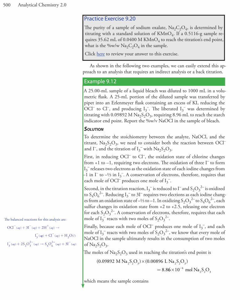
500 Analytical Chemistry 2.0
As shown in the following two examples, we can easily extend this ap-proach to an analysis that requires an indirect analysis or a back titration.
Example 9.12
A 25.00-mL sample of a liquid bleach was diluted to 1000 mL in a volu-metric flask. A 25-mL portion of the diluted sample was transferred by pipet into an Erlenmeyer flask containing an excess of KI, reducing the OCl– to Cl–, and producing I3
–. The liberated I3– was determined by
titrating with 0.09892 M Na2S2O3, requiring 8.96 mL to reach the starch indicator end point. Report the %w/v NaOCl in the sample of bleach.
Solution
To determine the stoichiometry between the analyte, NaOCl, and the titrant, Na2S2O3, we need to consider both the reaction between OCl– and I–, and the titration of I3
– with Na2S2O3. First, in reducing OCl– to Cl–, the oxidation state of chlorine changes from +1 to –1, requiring two electrons. The oxidation of three I– to form I3
– releases two electrons as the oxidation state of each iodine changes from –1 in I– to –⅓ in I3
–. A conservation of electrons, therefore, requires that each mole of OCl– produces one mole of I3
–.Second, in the titration reaction, I3
– is reduced to I– and S2O32– is oxidized
to S4O62–. Reducing I3
– to 3I– requires two elections as each iodine chang-es from an oxidation state of –⅓ to –1. In oxidizing S2O3
2– to S4O62–, each
sulfur changes its oxidation state from +2 to +2.5, releasing one electron for each S2O3
2–. A conservation of electrons, therefore, requires that each mole of I3
– reacts with two moles of S2O32–.
Finally, because each mole of OCl– produces one mole of I3–, and each
mole of I3– reacts with two moles of S2O3
2–, we know that every mole of NaOCl in the sample ultimately results in the consumption of two moles of Na2S2O3.The moles of Na2S2O3 used in reaching the titration’s end point is
( . ( .
.
0 09892 0 00896
8 8
M Na S O ) L Na S O )2 2 3 2 2 3�
= 66 10 4� − mol Na S O2 2 3
which means the sample contains
The balanced reactions for this analysis are:
OCl I H
I
− − +
−
+ + →( ) ( ) ( )
(
aq aq aq
a
3 2
3 qq aq l
aq aq
) ( ) ( )
( ) ( )
+ +
+ →
−
− −
Cl H O
I S O S O
2
2 43 32
622 −− −+( ) ( )aq aq3I
Practice Exercise 9.20The purity of a sample of sodium oxalate, Na2C2O4, is determined by titrating with a standard solution of KMnO4. If a 0.5116-g sample re-quires 35.62 mL of 0.0400 M KMnO4 to reach the titration’s end point, what is the %w/w Na2C2O4 in the sample.
Click here to review your answer to this exercise.

501Chapter 9 Titrimetric Methods
8 86 1014. � �− mol Na S O
mol NaOCl2 mol Na S2 2 3
2 22 3O
g NaOClmol NaOCl
g NaOCl
�
=74 44
0 03299.
.
Thus, the %w/v NaOCl in the diluted sample is
0 03299100 1 32
.. %
g NaOCl25.00 mL
w/v NaOCl� =
Because the bleach was diluted by a factor of 40 (25 mL to 1000 mL), the concentration of NaOCl in the bleach is 5.28% (w/v).
Example 9.13
The amount of ascorbic acid, C6H8O6, in orange juice was determined by oxidizing the ascorbic acid to dehydroascorbic acid, C6H6O6, with a known amount of I3
–, and back titrating the excess I3– with Na2S2O3.
A 5.00-mL sample of filtered orange juice was treated with 50.00 mL of 0.01023 M I3
–. After the oxidation was complete, 13.82 mL of 0.07203 M Na2S2O3 was needed to reach the starch indicator end point. Report the concentration ascorbic acid in mg/100 mL.
Solution
For a back titration we need to determine the stoichiometry between I3–
and the analyte, C6H8O6, and between I3– and the titrant, Na2S2O3. The
later is easy because we know from Example 9.12 that each mole of I3– re-
acts with two moles of Na2S2O3.In oxidizing ascorbic acid to dehydroascorbic acid, the oxidation state of carbon changes from +⅔ in C6H8O6 to +1 in C6H6O6. Each carbon releases ⅓ of an electron, or a total of two electrons per ascorbic acid. As we learned in Example 9.12, reducing I3
– requires two electrons; thus, a conservation of electrons requires that each mole of ascorbic acid con-sumes one mole of I3
–. The total moles of I3
– reacting with C6H8O6 and with Na2S2O3 is
( . ) ( . ) .0 01023 0 05000 5 115 10 4M I L I3 3− − −� = � mmol I3
−
The back titration consumes
0 013820 07203
..
L Na S Omol Na S O
L Na S2 2 32 2 3
2
�22 3
3
2 2 3
O
mol Imol Na S O
mol
�
= �−
−12
4 977 10 4. II3−
The balanced reactions for this analysis are:
C H O I
I C H O
6 8
6 6 6
6 3
3
( ) ( )
( ) ( )
aq aq
aq aq
+ →
+ +
−
− 22
2 33 32
62
H
I S O S O I2 4
+
− − − −+ → +
( )
( ) ( ) ( ) (
aq
aq aq aq aaq )

502 Analytical Chemistry 2.0
Subtracting the moles of I3– reacting with Na2S2O3 from the total moles
of I3– gives the moles reacting with ascorbic acid.
5 115 10 4 977 10 1 384 4. . .� − � = �− − − −mol I mol I3 3 110 5− −mol I3
The grams of ascorbic acid in the 5.00-mL sample of orange juice is
1 38 101
176 1
5.
.
� � �− −−
mol Imol C H O
mol I36 8 6
3
332 43 10 3g C H O
mol C H Og C H O6 8 6
6 8 66 8 6= � −.
There are 2.43 mg of ascorbic acid in the 5.00-mL sample, or 48.6 mg per 100 mL of orange juice.
Figure 9.42 Titration curve for the titra-tion of 50.0 mL of 0.0125 M Sn2+ and 0.0250 M Fe2+ with 0.050 M Ce4+. Both the titrand and the titrant are 1M in HCl.
Practice Exercise 9.21A quantitative analysis for ethanol, C2H6O, can be accomplished by a redox back titration. Ethanol is oxidized to acetic acid, C2H4O2, using excess dichromate, Cr2O7
2–, which is reduced to Cr3+. The excess dichro-mate is titrated with Fe2+, giving Cr3+ and Fe3+ as products. In a typical analysis, a 5.00-mL sample of a brandy is diluted to 500 mL in a volu-metric flask. A 10.00-mL sample is taken and the ethanol is removed by distillation and collected in 50.00 mL of an acidified solution of 0.0200 M K2Cr2O7. A back titration of the unreacted Cr2O7
2–requires 21.48 mL of 0.1014 M Fe2+. Calculate the %w/v ethanol in the brandy.
Click here to review your answer to this exercise.
9D.4 Evaluation of Redox Titrimetry
The scale of operations, accuracy, precision, sensitivity, time, and cost of a redox titration are similar to those described earlier in this chapter for acid–base or a complexation titration. As with acid–base titrations, we can extend a redox titration to the analysis of a mixture of analytes if there is a significant difference in their oxidation or reduction potentials. Figure 9.42 shows an example of the titration curve for a mixture of Fe2+ and Sn2+ using Ce4+ as the titrant. A titration of a mixture of analytes is possible if their standard state potentials or formal potentials differ by at least 200 mV.
9E Precipitation TitrationsThus far we have examined titrimetric methods based on acid–base, com-plexation, and redox reactions. A reaction in which the analyte and titrant form an insoluble precipitate also can serve as the basis for a titration. We call this type of titration a precipitation titration.
One of the earliest precipitation titrations—developed at the end of the eighteenth century—was the analysis of K2CO3 and K2SO4 in potash.
0 10 20 30 40 50 60 70
0.2
0.4
0.6
0.8
1.0
1.2
Volume of Ce4+ (mL)
E (V
)
end point for Sn2+
end point for Fe2+
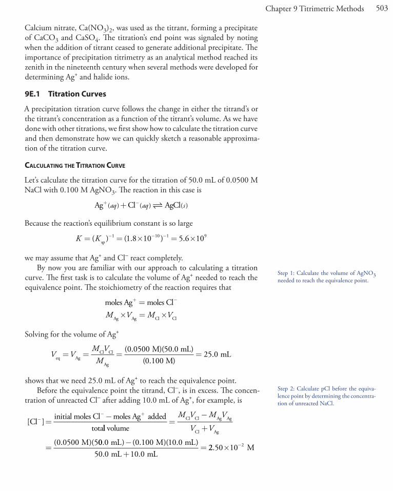
503Chapter 9 Titrimetric Methods
Calcium nitrate, Ca(NO3)2, was used as the titrant, forming a precipitate of CaCO3 and CaSO4. The titration’s end point was signaled by noting when the addition of titrant ceased to generate additional precipitate. The importance of precipitation titrimetry as an analytical method reached its zenith in the nineteenth century when several methods were developed for determining Ag+ and halide ions.
9E.1 Titration Curves
A precipitation titration curve follows the change in either the titrand’s or the titrant’s concentration as a function of the titrant’s volume. As we have done with other titrations, we first show how to calculate the titration curve and then demonstrate how we can quickly sketch a reasonable approxima-tion of the titration curve.
calculaTing The TiTraTion curve
Let’s calculate the titration curve for the titration of 50.0 mL of 0.0500 M NaCl with 0.100 M AgNO3. The reaction in this case is
Ag Cl AgCl+ −+( ) ( ) ( )aq aq s
Because the reaction’s equilibrium constant is so large
K K= = � = �− − −( ) ( . ) .sp1 10 1 91 8 10 5 6 10
we may assume that Ag+ and Cl– react completely.By now you are familiar with our approach to calculating a titration
curve. The first task is to calculate the volume of Ag+ needed to reach the equivalence point. The stoichiometry of the reaction requires that
moles Ag moles Cl
Ag Ag Cl Cl
+ −=
� = �M V M V
Solving for the volume of Ag+
V VM V
Meq AgCl Cl
Ag
M)(50.0 mL)(0.100
= = =( .0 0500
M)mL= 25 0.
shows that we need 25.0 mL of Ag+ to reach the equivalence point.Before the equivalence point the titrand, Cl–, is in excess. The concen-
tration of unreacted Cl– after adding 10.0 mL of Ag+, for example, is
[ ]Clinitial moles Cl moles Ag added
tota−
− +
=−
ll volume
M
Cl Cl Ag Ag
Cl Ag
=−
+
=
M V M V
V V
( . )(0 0500 500 0 0 100 10 050 0 10 0
. ) ( . )( . )
. .mL M mLmL mL
−+
= 22 50 10 2. � − M
Step 1: Calculate the volume of AgNO3 needed to reach the equivalence point.
Step 2: Calculate pCl before the equiva-lence point by determining the concentra-tion of unreacted NaCl.

504 Analytical Chemistry 2.0
which corresponds to a pCl of 1.60.At the titration’s equivalence point, we know that the concentrations
of Ag+ and Cl– are equal. To calculate the concentration of Cl– we use the Ksp expression for AgCl; thus
K x xsp Ag Cl= = = �+ − −[ ][ ] ( )( ) .1 8 10 10
Solving for x gives [Cl–] as 1.3 � 10–5 M, or a pCl of 4.89.After the equivalence point, the titrant is in excess. We first calculate the
concentration of excess Ag+ and then use the Ksp expression to calculate the concentration of Cl–. For example, after adding 35.0 mL of titrant
[ ]Agmoles Ag added initial moles Cl
tota+
+ −
=−
ll volume
M
Ag Ag Cl Cl
Cl Ag
=−
+
=
M V M V
V V
( . )(0 100 35.. ) ( . )( . ). .
0 0 0500 50 050 0 35 0
mL M mLmL mL−+
=11 18 10 2. � − M
[ ][ ]
..
.ClAg
Msp−+
−
−−= =
��
= �K 1 8 10
1 18 101 5 10
10
28
or a pCl of 7.81. Additional results for the titration curve are shown in Table 9.18 and Figure 9.43.
Table 9.18 Titration of 50.0 mL of 0.0500 M NaCl with 0.100 M AgNO3
Volume of AgNO3 (mL) pCl Volume of AgNO3 (mL) pCl0.00 1.30 30.0 7.545.00 1.44 35.0 7.82
10.0 1.60 40.0 7.9715.0 1.81 45.0 8.0720.0 2.15 50.0 8.1425.0 4.89
Figure 9.43 Titration curve for the titration of 50.0 mL of 0.0500 M NaCl with 0.100 M AgNO3. The red points corresponds to the data in Table 9.18. The blue line shows the complete titration curve.
Step 3: Calculate pCl at the equivalence point using the Ksp for AgCl to calculate the concentration of Cl–.
Step 4: Calculate pCl after the equivalence point by first calculating the concentra-tion of excess AgNO3 and then calculat-ing the concentration of Cl– using the Ksp for AgCl.
0 10 20 30 40 50
0
2
4
6
8
10
Volume of AgNO3
pCl
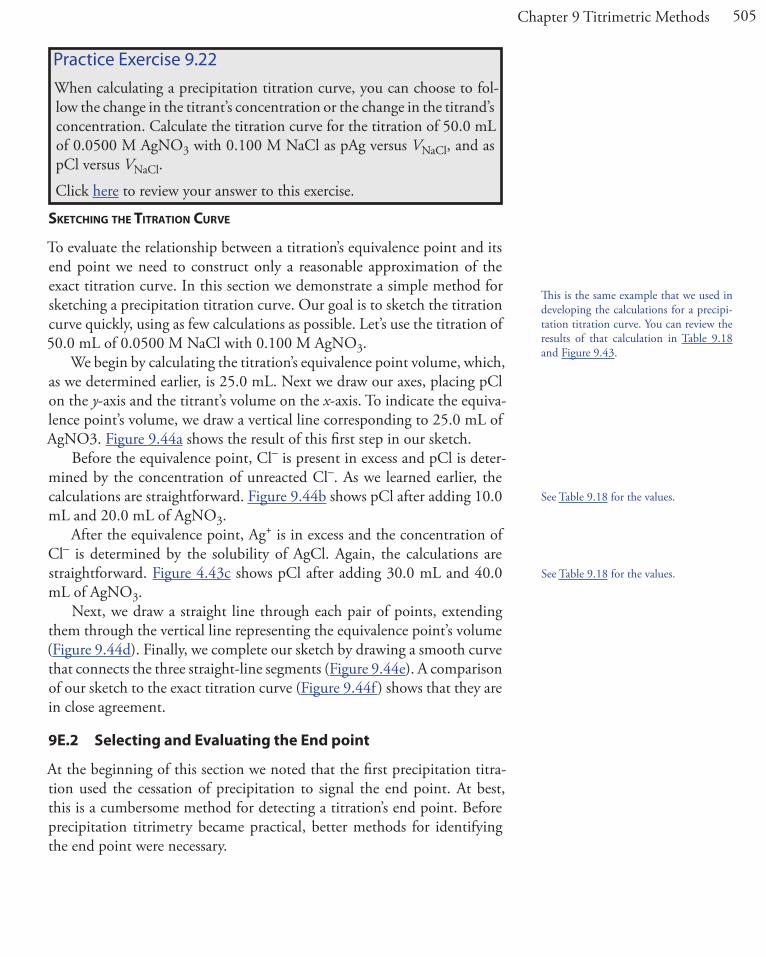
505Chapter 9 Titrimetric Methods
SkeTching The TiTraTion curve
To evaluate the relationship between a titration’s equivalence point and its end point we need to construct only a reasonable approximation of the exact titration curve. In this section we demonstrate a simple method for sketching a precipitation titration curve. Our goal is to sketch the titration curve quickly, using as few calculations as possible. Let’s use the titration of 50.0 mL of 0.0500 M NaCl with 0.100 M AgNO3.
We begin by calculating the titration’s equivalence point volume, which, as we determined earlier, is 25.0 mL. Next we draw our axes, placing pCl on the y-axis and the titrant’s volume on the x-axis. To indicate the equiva-lence point’s volume, we draw a vertical line corresponding to 25.0 mL of AgNO3. Figure 9.44a shows the result of this first step in our sketch.
Before the equivalence point, Cl– is present in excess and pCl is deter-mined by the concentration of unreacted Cl–. As we learned earlier, the calculations are straightforward. Figure 9.44b shows pCl after adding 10.0 mL and 20.0 mL of AgNO3.
After the equivalence point, Ag+ is in excess and the concentration of Cl– is determined by the solubility of AgCl. Again, the calculations are straightforward. Figure 4.43c shows pCl after adding 30.0 mL and 40.0 mL of AgNO3.
Next, we draw a straight line through each pair of points, extending them through the vertical line representing the equivalence point’s volume (Figure 9.44d). Finally, we complete our sketch by drawing a smooth curve that connects the three straight-line segments (Figure 9.44e). A comparison of our sketch to the exact titration curve (Figure 9.44f ) shows that they are in close agreement.
9E.2 Selecting and Evaluating the End point
At the beginning of this section we noted that the first precipitation titra-tion used the cessation of precipitation to signal the end point. At best, this is a cumbersome method for detecting a titration’s end point. Before precipitation titrimetry became practical, better methods for identifying the end point were necessary.
Practice Exercise 9.22When calculating a precipitation titration curve, you can choose to fol-low the change in the titrant’s concentration or the change in the titrand’s concentration. Calculate the titration curve for the titration of 50.0 mL of 0.0500 M AgNO3 with 0.100 M NaCl as pAg versus VNaCl, and as pCl versus VNaCl.
Click here to review your answer to this exercise.
This is the same example that we used in developing the calculations for a precipi-tation titration curve. You can review the results of that calculation in Table 9.18 and Figure 9.43.
See Table 9.18 for the values.
See Table 9.18 for the values.

506 Analytical Chemistry 2.0
Figure 9.44 Illustrations showing the steps in sketching an approximate titration curve for the titration of 50.0 mL of 0.0500 M NaCl with 0.100 M AgNO3: (a) locating the equivalence point volume; (b) plotting two points before the equivalence point; (c) plotting two points after the equivalence point; (d) preliminary approximation of titration curve using straight-lines; (e) final approximation of titration curve using a smooth curve; (f ) com-parison of approximate titration curve (solid black line) and exact titration curve (dashed red line). See the text for additional details. A better fit is possible if the two points before the equivalence point are further apart—for example, 0 mL and 20 mL— and the two points after the equivalence point are further apart.
0 10 20 30 40 50
0
2
4
6
8
10
Volume of AgNO3
pCl
(a)
0 10 20 30 40 50
0
2
4
6
8
10
Volume of AgNO3
pCl
(b)
0 10 20 30 40 50
0
2
4
6
8
10
Volume of AgNO3
pCl
(c)
0 10 20 30 40 50
0
2
4
6
8
10
Volume of AgNO3
pCl
(d)
0 10 20 30 40 50
0
2
4
6
8
10
Volume of AgNO3
pCl
(e)
0 10 20 30 40 50
0
2
4
6
8
10
Volume of AgNO3
pCl
(f )

507Chapter 9 Titrimetric Methods
Finding The end PoinT WiTh an indicaTor
There are three general types of indicators for precipitation titrations, each of which changes color at or near the titration’s equivalence point. The first type of indicator is a species that forms a precipitate with the titrant. In the Mohr method for Cl– using Ag+ as a titrant, for example, a small amount of K2CrO4 is added to the titrand’s solution. The titration’s end point is the formation of a reddish-brown precipitate of Ag2CrO4.
Because CrO42– imparts a yellow color to the solution, which might
obscure the end point, only a small amount of K2CrO4 is added. As a result, the end point is always later than the equivalence point. To compensate for this positive determinate error, an analyte-free reagent blank is analyzed to determine the volume of titrant needed to affect a change in the indicator’s color. Subtracting the end point for the reagent blank from the titrand’s end point gives the titration’s end point. Because CrO4
2– is a weak base, the titrand’s solution is made slightly alkaline. If the pH is too acidic, chromate is present as HCrO4
– instead of CrO42–, and the Ag2CrO4 end point is
delayed. The pH also must be less than 10 to avoid the precipitation of silver hydroxide.
A second type of indicator uses a species that forms a colored complex with the titrant or the titrand. In the Volhard method for Ag+ using KSCN as the titrant, for example, a small amount of Fe3+ is added to the titrand’s solution. The titration’s end point is the formation of the reddish-colored Fe(SCN)2+ complex. The titration must be carried out in an acidic solution to prevent the precipitation of Fe3+ as Fe(OH)3.
The third type of end point uses a species that changes color when it adsorbs to the precipitate. In the Fajans method for Cl– using Ag+ as a titrant, for example, the anionic dye dichlorofluoroscein is added to the titrand’s solution. Before the end point, the precipitate of AgCl has a nega-tive surface charge due to the adsorption of excess Cl–. Because dichloro-fluoroscein also carries a negative charge, it is repelled by the precipitate and remains in solution where it has a greenish-yellow color. After the end point, the surface of the precipitate carries a positive surface charge due to the adsorption of excess Ag+. Dichlorofluoroscein now adsorbs to the precipitate’s surface where its color is pink. This change in the indicator’s color signals the end point.
Finding The end PoinT PoTenTioMeTrically
Another method for locating the end point is a potentiometric titration in which we monitor the change in the titrant’s or the titrand’s concentration using an ion-selective electrode. The end point is found by visually examin-ing the titration curve. A further discussion of potentiometry is found in Chapter 11.
The Mohr method was first published in 1855 by Karl Friedrich Mohr.
The Volhard method was first published in 1874 by Jacob Volhard.
The Fajans method was first published in the 1920s by Kasimir Fajans.

508 Analytical Chemistry 2.0
9E.3 Quantitative Applications
Although precipitation titrimetry is rarely listed as a standard method of analysis, it may still be useful as a secondary analytical method for verifying other analytical methods. Most precipitation titrations use Ag+ as either the titrand or the titration. A titration in which Ag+ is the titrant is called an arGentometric titration. Table 9.19 provides a list of several typical precipitation titrations.
quanTiTaTive calculaTionS
The quantitative relationship between the titrand and the titrant is deter-mined by the stoichiometry of the titration reaction. If you are unsure of the balanced reaction, you can deduce the stoichiometry from the pre-cipitate’s formula. For example, in forming a precipitate of Ag2CrO4, each mole of CrO4
2– reacts with two moles of Ag+.
Example 9.14
A mixture containing only KCl and NaBr is analyzed by the Mohr method. A 0.3172-g sample is dissolved in 50 mL of water and titrated to the Ag2CrO4 end point, requiring 36.85 mL of 0.1120 M AgNO3. A blank titration requires 0.71 mL of titrant to reach the same end point. Report the %w/w KCl in the sample.
Table 9.19 Representative Examples of Precipitation Titrations
Titrand Titranta End Pointb
AsO43– AgNO3, KSCN Volhard
Br– AgNO3AgNO3, KSCN
Mohr or FajansVolhard
Cl– AgNO3AgNO3, KSCN
Mohr or FajansVolhard*
CO32– AgNO3, KSCN Volhard*
C2O42– AgNO3, KSCN Volhard*
CrO42– AgNO3, KSCN Volhard*
I– AgNO3AgNO3, KSCN
FajansVolhard
PO43– AgNO3, KSCN Volhard*
S2– AgNO3, KSCN Volhard*SCN– AgNO3, KSCN Volhard*
a When two reagents are listed, the analysis is by a back titration. The first re-agent is added in excess and the second reagent used to back titrate the excess.
b For those Volhard methods identified with an asterisk (*) the precipitated silver salt must be removed before carrying out the back titration.

509Chapter 9 Titrimetric Methods
Solution
To find the moles of titrant reacting with the sample, we first need to cor-rect for the reagent blank; thus
VAg mL mL mL= − =36 85 0 71 36 14. . .
(0.1120 M AgNO ) L AgNO )3 3� = �( . .0 03614 4 048 10−−3 mol AgNO3
Titrating with AgNO3 produces a precipitate of AgCl and AgBr. In form-ing the precipitates, each mole of KCl consumes one mole of AgNO3 and each mole of NaBr consumes one mole of AgNO3; thus
moles KCl moles NaBr+ = � −4 048 10 3.
We are interested in finding the mass of KCl, so let’s rewrite this equation in terms of mass. We know that
moles KClg KCl
74.551 g KCl/mol KCl
moles N
=
aaBrg NaBr
102.89 g NaBr/mol NaBr=
which we substitute back into the previous equation
g KCl74.551 g KCl/mol KCl
g NaBr102.89 g Na
+BBr/mol NaBr
= � −4 048 10 3.
Because this equation has two unknowns—g KCl and g NaBr—we need another equation that includes both unknowns. A simple equation takes advantage of the fact that the sample contains only KCl and NaBr; thus,
g NaBr g g KCl= −0 3172.
g KCl74.551 g KCl/mol KCl
g g KCl102
+−0 3172.
..89 g NaBr/mol NaBr= � −4 048 10 3.
1 341 10 3 083 10 9 719 102 3 3. . . (� + � − �− − −(g KCl) g KCCl)= � −4 048 10 3.
3 69 10 9 65 103 4. .� = �− −(g KCl)
The sample contains 0.262 g of KCl and the %w/w KCl in the sample is
0 2620 3172
100 82 6.
.. %
g KClg sample
w/w KC� = ll
The analysis for I– using the Volhard method requires a back titration. A typical calculation is shown in the following example.
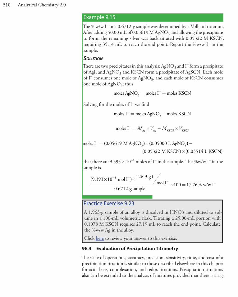
510 Analytical Chemistry 2.0
Example 9.15
The %w/w I– in a 0.6712-g sample was determined by a Volhard titration. After adding 50.00 mL of 0.05619 M AgNO3 and allowing the precipitate to form, the remaining silver was back titrated with 0.05322 M KSCN, requiring 35.14 mL to reach the end point. Report the %w/w I– in the sample.
Solution
There are two precipitates in this analysis: AgNO3 and I– form a precipitate of AgI, and AgNO3 and KSCN form a precipitate of AgSCN. Each mole of I– consumes one mole of AgNO3, and each mole of KSCN consumes one mole of AgNO3; thus
moles AgNO moles I moles KSCN3 = +−
Solving for the moles of I– we find
moles I moles AgNO moles KSCN3− = −
moles I Ag Ag KSCN KSCN− = � − �M V M V
moles I M AgNO ) 0 L AgNO3 3− = �( . ( .0 05619 0 0500 ))
M KSCN) L KSCN)
−
�( . ( .0 05322 0 03514
that there are 9.393 � 10–4 moles of I– in the sample. The %w/w I– in the sample is
( . ) .
.
9 393 10 126 9
0 6712
4� �− −−
−mol I g Imol I
gg samplew/w I� = −100 17 76. %
Practice Exercise 9.23A 1.963-g sample of an alloy is dissolved in HNO3 and diluted to vol-ume in a 100-mL volumetric flask. Titrating a 25.00-mL portion with 0.1078 M KSCN requires 27.19 mL to reach the end point. Calculate the %w/w Ag in the alloy.
Click here to review your answer to this exercise.
9E.4 Evaluation of Precipitation Titrimetry
The scale of operations, accuracy, precision, sensitivity, time, and cost of a precipitation titration is similar to those described elsewhere in this chapter for acid–base, complexation, and redox titrations. Precipitation titrations also can be extended to the analysis of mixtures provided that there is a sig-

511Chapter 9 Titrimetric Methods
nificant difference in the solubilities of the precipitates. Figure 9.45 shows an example of a titration curve for a mixture of I– and Cl– using Ag+ as a titrant.
9F Key Termsacid–base titration acidity alkalinityargentometric titration asymmetric equivalence
pointauxiliary complexing agent
auxiliary oxidizing agent auxiliary reducing agent back titrationburet complexation titration conditional formation
constantdirect titration displacement titration end pointequivalence point Fajans method formal potentialGran plot indicator Jones reductorKjeldahl analysis leveling metallochromic indicatorMohr method potentiometric titration precipitation titrationredox indicator redox titration spectrophotometric
titrationsymmetric equivalence point
thermometric titration titrand
titrant titration curve titration errortitrimetry Volhard method Walden reductor
9G Chapter SummaryIn a titrimetric method of analysis, the volume of titrant reacting stoi-chiometrically with a titrand provides quantitative information about the amount of analyte in a sample. The volume of titrant corresponding to this stoichiometric reaction is called the equivalence point. Experimentally we determine the titration’s end point using an indicator that changes color near the equivalence point. Alternatively, we can locate the end point by
Figure 9.45 Titration curve for the titration of a 50.0 mL mixture of 0.0500 M I– and 0.0500 M Cl– using 0.100 M Ag+ as a titrant. The red arrows show the end points. Note that the end point for I– is earlier than the end point for Cl– because AgI is less soluble than AgCl.
0 20 40 60 80
0
5
10
15
Volume of AgNO3 (mL)
pAg
end point for I–
end point for Cl–
As you review this chapter, try to define a key term in your own words. Check your answer by clicking on the key term, which will take you to the page where it was first introduced. Clicking on the key term there, will bring you back to this page so that you can continue with another key term.

512 Analytical Chemistry 2.0
continuously monitoring a property of the titrand’s solution—absorbance, potential, and temperature are typical examples—that changes as the titra-tion progresses. In either case, an accurate result requires that the end point closely match the equivalence point. Knowing the shape of a titration curve is critical to evaluating the feasibility of a titrimetric method.
Many titrations are direct, in which the analyte participates in the titra-tion as the titrand or the titrant. Other titration strategies may be used when a direct reaction between the analyte and titrant is not feasible. In a back titration a reagent is added in excess to a solution containing the analyte. When the reaction between the reagent and the analyte is complete, the amount of excess reagent is determined by a titration. In a displacement titration the analyte displaces a reagent, usually from a complex, and the amount of displaced reagent is determined by an appropriate titration.
Titrimetric methods have been developed using acid–base, complex-ation, redox, and precipitation reactions. Acid–base titrations use a strong acid or a strong base as a titrant. The most common titrant for a compl-exation titration is EDTA. Because of their stability against air oxidation, most redox titrations use an oxidizing agent as a titrant. Titrations with reducing agents also are possible. Precipitation titrations often involve Ag+ as either the analyte or titrant.
9H Problems
1. Calculate or sketch titration curves for the following acid–base titra-tions.
a. 25.0 mL of 0.100 M NaOH with 0.0500 M HCl
b. 50.0 mL of 0.0500 M HCOOH with 0.100 M NaOH
c. 50.0 mL of 0.100 M NH3 with 0.100 M HCl
d. 50.0 mL of 0.0500 M ethylenediamine with 0.100 M HCl
e. 50.0 mL of 0.0400 M citric acid with 0.120 M NaOH
f. 50.0 mL of 0.0400 M H3PO4 with 0.120 M NaOH
2. Locate the equivalence point for each titration curve in problem 1. What is the stoichiometric relationship between the moles of acid and the moles of base at each of these equivalence points?
3. Suggest an appropriate visual indicator for each of the titrations in problem 1.
4. In sketching the titration curve for a weak acid we approximate the pH at 10% of the equivalence point volume as pKa – 1, and the pH at 90% of the equivalence point volume as pKa + 1. Show that these assump-tions are reasonable.
Some of the problems that follow require one or more equilibrium constants or standard state po-tentials. For your convenience, here are hyperlinks to the appendices containing these constants
Appendix 10: Solubility Products
Appendix 11: Acid Dissociation Constants
Appendix 12: Metal-Ligand Formation Constants
Appendix 13: Standard State Reduction Potentials
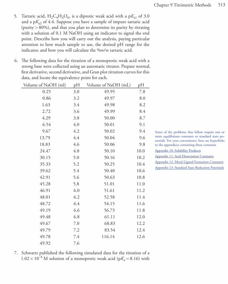
513Chapter 9 Titrimetric Methods
5. Tartaric acid, H2C4H4O6, is a diprotic weak acid with a pKa1 of 3.0 and a pKa2 of 4.4. Suppose you have a sample of impure tartaric acid (purity > 80%), and that you plan to determine its purity by titrating with a solution of 0.1 M NaOH using an indicator to signal the end point. Describe how you will carry out the analysis, paying particular attention to how much sample to use, the desired pH range for the indicator, and how you will calculate the %w/w tartaric acid.
6. The following data for the titration of a monoprotic weak acid with a strong base were collected using an automatic titrator. Prepare normal, first derivative, second derivative, and Gran plot titration curves for this data, and locate the equivalence point for each.Volume of NaOH (ml) pH Volume of NaOH (mL) pH
0.25 3.0 49.95 7.80.86 3.2 49.97 8.01.63 3.4 49.98 8.22.72 3.6 49.99 8.44.29 3.8 50.00 8.76.54 4.0 50.01 9.19.67 4.2 50.02 9.4
13.79 4.4 50.04 9.618.83 4.6 50.06 9.824.47 4.8 50.10 10.030.15 5.0 50.16 10.235.33 5.2 50.25 10.439.62 5.4 50.40 10.642.91 5.6 50.63 10.845.28 5.8 51.01 11.046.91 6.0 51.61 11.248.01 6.2 52.58 11.448.72 6.4 54.15 11.649.19 6.6 56.73 11.849.48 6.8 61.11 12.049.67 7.0 68.83 12.249.79 7.2 83.54 12.449.78 7.4 116.14 12.649.92 7.6
7. Schwartz published the following simulated data for the titration of a 1.02 � 10–4 M solution of a monoprotic weak acid (pKa = 8.16) with
Some of the problems that follow require one or more equilibrium constants or standard state po-tentials. For your convenience, here are hyperlinks to the appendices containing these constants
Appendix 10: Solubility Products
Appendix 11: Acid Dissociation Constants
Appendix 12: Metal-Ligand Formation Constants
Appendix 13: Standard State Reduction Potentials

514 Analytical Chemistry 2.0
1.004 � 10–3 M NaOH.10 The simulation assumes that a 50-mL pipet is used to transfer a portion of the weak acid solution to the titration vessel. A calibration of the pipet shows that it delivers a volume of only 49.94 mL. Prepare normal, first derivative, second derivative, and Gran plot titration curves for this data, and determine the equivalence point for each. How do these equivalence points compare to the expected equivalence point? Comment on the utility of each titration curve for the analysis of very dilute solutions of very weak acids.
mL of NaOH pH mL of NaOH pH0.03 6.212 4.79 8.8580.09 6.504 4.99 8.9260.29 6.936 5.21 8.9940.72 7.367 5.41 9.0561.06 7.567 5.61 9.1181.32 7.685 5.85 9.1801.53 7.776 6.05 9.2311.76 7.863 6.28 9.2831.97 7.938 6.47 9.3272.18 8.009 6.71 9.3742.38 8.077 6.92 9.4142.60 8.146 7.15 9.4512.79 8.208 7.36 9.4843.01 8.273 7.56 9.5143.41 8.332 7.79 9.5453.60 8.458 8.21 9.5723.80 8.521 8.44 9.5993.99 8.584 8.64 9.6454.18 8.650 8.84 9.6664.40 8.720 9.07 9.6884.57 8.784 9.27 9.706
8. Calculate or sketch the titration curve for a 50.0 mL solution of a 0.100 M monoprotic weak acid (pKa = 8) with 0.1 M strong base in a nonaqueous solvent with Ks = 10–20. You may assume that the change in solvent does not affect the weak acid’s pKa. Compare your titration curve to the titration curve when water is the solvent.
9. The titration of a mixture of p-nitrophenol (pKa = 7.0) and m-nitrop-henol (pKa = 8.3) can be followed spectrophotometrically. Neither acid absorbs at a wavelength of 545 nm, but their respective conjugate bases
10 Schwartz, L. M. J. Chem. Educ. 1992, 69, 879–883.
Some of the problems that follow require one or more equilibrium constants or standard state po-tentials. For your convenience, here are hyperlinks to the appendices containing these constants
Appendix 10: Solubility Products
Appendix 11: Acid Dissociation Constants
Appendix 12: Metal-Ligand Formation Constants
Appendix 13: Standard State Reduction Potentials
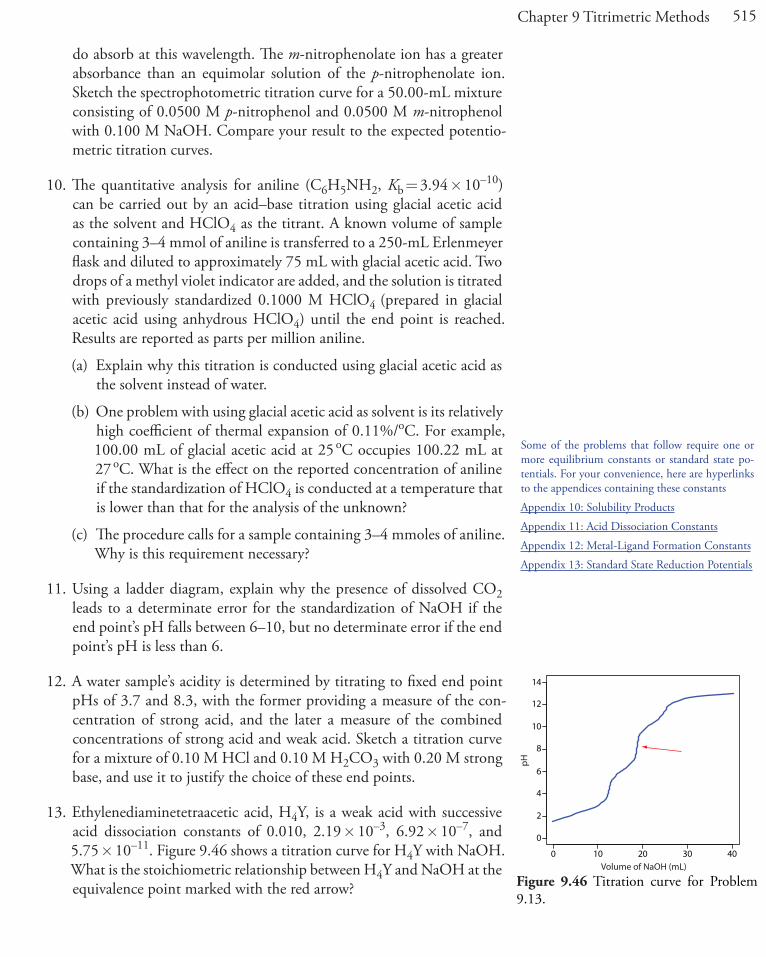
515Chapter 9 Titrimetric Methods
do absorb at this wavelength. The m-nitrophenolate ion has a greater absorbance than an equimolar solution of the p-nitrophenolate ion. Sketch the spectrophotometric titration curve for a 50.00-mL mixture consisting of 0.0500 M p-nitrophenol and 0.0500 M m-nitrophenol with 0.100 M NaOH. Compare your result to the expected potentio-metric titration curves.
10. The quantitative analysis for aniline (C6H5NH2, Kb = 3.94 � 10–10) can be carried out by an acid–base titration using glacial acetic acid as the solvent and HClO4 as the titrant. A known volume of sample containing 3–4 mmol of aniline is transferred to a 250-mL Erlenmeyer flask and diluted to approximately 75 mL with glacial acetic acid. Two drops of a methyl violet indicator are added, and the solution is titrated with previously standardized 0.1000 M HClO4 (prepared in glacial acetic acid using anhydrous HClO4) until the end point is reached. Results are reported as parts per million aniline.
(a) Explain why this titration is conducted using glacial acetic acid as the solvent instead of water.
(b) One problem with using glacial acetic acid as solvent is its relatively high coefficient of thermal expansion of 0.11%/oC. For example, 100.00 mL of glacial acetic acid at 25 oC occupies 100.22 mL at 27 oC. What is the effect on the reported concentration of aniline if the standardization of HClO4 is conducted at a temperature that is lower than that for the analysis of the unknown?
(c) The procedure calls for a sample containing 3–4 mmoles of aniline. Why is this requirement necessary?
11. Using a ladder diagram, explain why the presence of dissolved CO2 leads to a determinate error for the standardization of NaOH if the end point’s pH falls between 6–10, but no determinate error if the end point’s pH is less than 6.
12. A water sample’s acidity is determined by titrating to fixed end point pHs of 3.7 and 8.3, with the former providing a measure of the con-centration of strong acid, and the later a measure of the combined concentrations of strong acid and weak acid. Sketch a titration curve for a mixture of 0.10 M HCl and 0.10 M H2CO3 with 0.20 M strong base, and use it to justify the choice of these end points.
13. Ethylenediaminetetraacetic acid, H4Y, is a weak acid with successive acid dissociation constants of 0.010, 2.19 � 10–3, 6.92 � 10–7, and 5.75 � 10–11. Figure 9.46 shows a titration curve for H4Y with NaOH. What is the stoichiometric relationship between H4Y and NaOH at the equivalence point marked with the red arrow?
Some of the problems that follow require one or more equilibrium constants or standard state po-tentials. For your convenience, here are hyperlinks to the appendices containing these constants
Appendix 10: Solubility Products
Appendix 11: Acid Dissociation Constants
Appendix 12: Metal-Ligand Formation Constants
Appendix 13: Standard State Reduction Potentials
0 10 20 30 40
0
2
4
6
8
10
12
14
pH
Volume of NaOH (mL)
Figure 9.46 Titration curve for Problem 9.13.
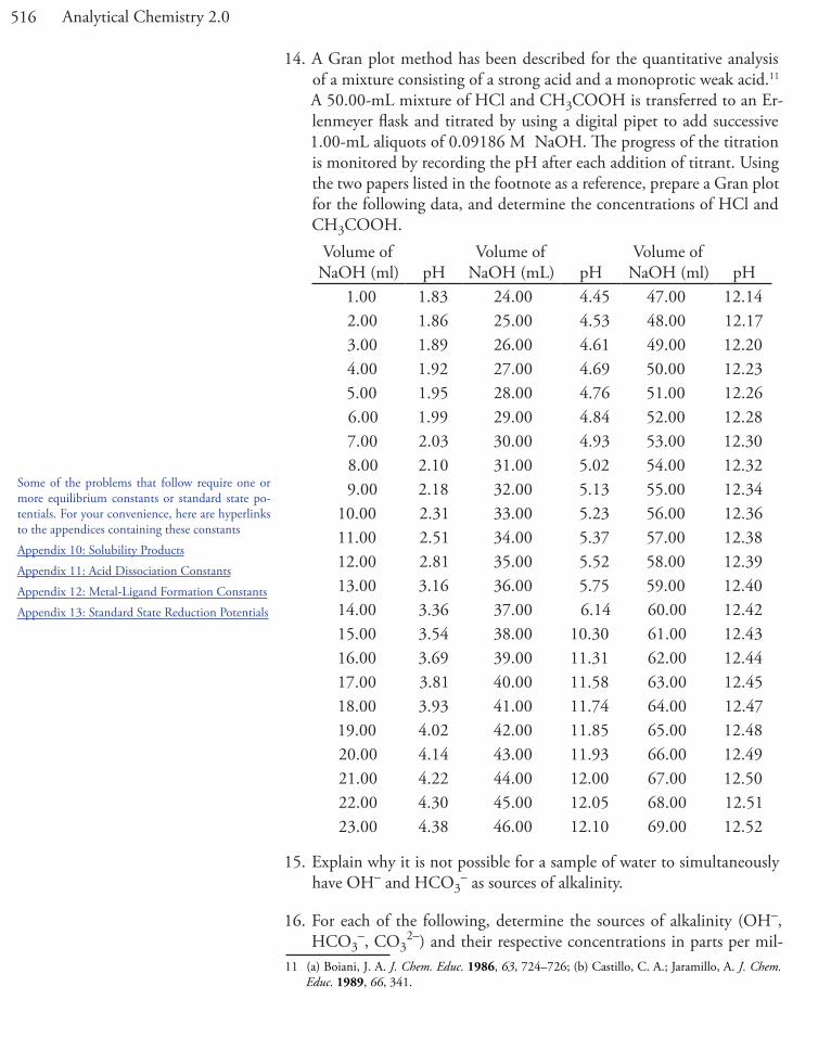
516 Analytical Chemistry 2.0
14. A Gran plot method has been described for the quantitative analysis of a mixture consisting of a strong acid and a monoprotic weak acid.11 A 50.00-mL mixture of HCl and CH3COOH is transferred to an Er-lenmeyer flask and titrated by using a digital pipet to add successive 1.00-mL aliquots of 0.09186 M NaOH. The progress of the titration is monitored by recording the pH after each addition of titrant. Using the two papers listed in the footnote as a reference, prepare a Gran plot for the following data, and determine the concentrations of HCl and CH3COOH.
Volume of NaOH (ml) pH
Volume of NaOH (mL) pH
Volume of NaOH (ml) pH
1.00 1.83 24.00 4.45 47.00 12.142.00 1.86 25.00 4.53 48.00 12.173.00 1.89 26.00 4.61 49.00 12.204.00 1.92 27.00 4.69 50.00 12.235.00 1.95 28.00 4.76 51.00 12.266.00 1.99 29.00 4.84 52.00 12.287.00 2.03 30.00 4.93 53.00 12.308.00 2.10 31.00 5.02 54.00 12.329.00 2.18 32.00 5.13 55.00 12.34
10.00 2.31 33.00 5.23 56.00 12.3611.00 2.51 34.00 5.37 57.00 12.3812.00 2.81 35.00 5.52 58.00 12.3913.00 3.16 36.00 5.75 59.00 12.4014.00 3.36 37.00 6.14 60.00 12.4215.00 3.54 38.00 10.30 61.00 12.4316.00 3.69 39.00 11.31 62.00 12.4417.00 3.81 40.00 11.58 63.00 12.4518.00 3.93 41.00 11.74 64.00 12.4719.00 4.02 42.00 11.85 65.00 12.4820.00 4.14 43.00 11.93 66.00 12.4921.00 4.22 44.00 12.00 67.00 12.5022.00 4.30 45.00 12.05 68.00 12.5123.00 4.38 46.00 12.10 69.00 12.52
15. Explain why it is not possible for a sample of water to simultaneously have OH– and HCO3
– as sources of alkalinity.
16. For each of the following, determine the sources of alkalinity (OH–, HCO3
–, CO32–) and their respective concentrations in parts per mil-
11 (a) Boiani, J. A. J. Chem. Educ. 1986, 63, 724–726; (b) Castillo, C. A.; Jaramillo, A. J. Chem. Educ. 1989, 66, 341.
Some of the problems that follow require one or more equilibrium constants or standard state po-tentials. For your convenience, here are hyperlinks to the appendices containing these constants
Appendix 10: Solubility Products
Appendix 11: Acid Dissociation Constants
Appendix 12: Metal-Ligand Formation Constants
Appendix 13: Standard State Reduction Potentials
517Chapter 9 Titrimetric Methods
lion In each case a 25.00-mL sample is titrated with 0.1198 M HCl to the bromocresol green and the phenolphthalein end points.
Volume of HCl (mL) to the phenolphthalein end point
Volume of HCl (mL) to the bromocresol green end point
a 21.36 21.38b 5.67 21.13c 0.00 14.28d 17.12 34.26e 21.36 25.69
17. A sample may contain any of the following: HCl, NaOH, H3PO4, H2PO4
–, HPO42–, or PO4
3–. The composition of a sample is deter-mined by titrating a 25.00-mL portion with 0.1198 M HCl or 0.1198 M NaOH to the phenolphthalein and the methyl orange end points. For each of the following, determine which species are present in the sample, and their respective molar concentrations.
TitrantPhenolphthalein end point volume (mL)
methyl orange end point volume (mL)
a HCl 11.54 35.29b NaOH 19.79 9.89c HCl 22.76 22.78d NaOH 39.42 17.48
18. The protein in a 1.2846-g sample of an oat cereal is determined by a Kjeldahl analysis. The sample is digested with H2SO4, the resulting solution made basic with NaOH, and the NH3 distilled into 50.00 mL of 0.09552 M HCl. The excess HCl is back titrated using 37.84 mL of 0.05992 M NaOH. Given that the proteins in grains average 17.54% w/w N, report the %w/w protein in the sample.
19. The concentration of SO2 in air is determined by bubbling a sample of air through a trap containing H2O2. Oxidation of SO2 by H2O2 results in the formation of H2SO4, which is then determined by titrating with NaOH. In a typical analysis, a sample of air was passed through the peroxide trap at a rate of 12.5 L/min for 60 min and required 10.08 mL of 0.0244 M NaOH to reach the phenolphthalein end point. Calculate the mL/L SO2 in the sample of air. The density of SO2 at the tempera-ture of the air sample is 2.86 mg/mL.
20. The concentration of CO2 in air is determined by an indirect acid–base titration. A sample of air is bubbled through a solution containing an excess of Ba(OH)2, precipitating BaCO3. The excess Ba(OH)2 is back titrated with HCl. In a typical analysis a 3.5-L sample of air was bubbled through 50.00 mL of 0.0200 M Ba(OH)2. Back titrating with
Some of the problems that follow require one or more equilibrium constants or standard state po-tentials. For your convenience, here are hyperlinks to the appendices containing these constants
Appendix 10: Solubility Products
Appendix 11: Acid Dissociation Constants
Appendix 12: Metal-Ligand Formation Constants
Appendix 13: Standard State Reduction Potentials

518 Analytical Chemistry 2.0
0.0316 M HCl required 38.58 mL to reach the end point. Determine the ppm CO2 in the sample of air given that the density of CO2 at the temperature of the sample is 1.98 g/L.
21. The purity of a synthetic preparation of methylethyl ketone, C3H8O, is determined by reacting it with hydroxylamine hydrochloride, liberating HCl (see reaction in Table 9.8). In a typical analysis a 3.00-mL sample was diluted to 50.00 mL and treated with an excess of hydroxylamine hydrochloride. The liberated HCl was titrated with 0.9989 M NaOH, requiring 32.68 mL to reach the end point. Report the percent purity of the sample given that the density of methylethyl ketone is 0.805 g/mL.
22. Animal fats and vegetable oils are triesters formed from the reaction between glycerol (1,2,3-propanetriol) and three long-chain fatty acids. One of the methods used to characterize a fat or an oil is a determina-tion of its saponification number. When treated with boiling aqueous KOH, an ester saponifies into the parent alcohol and fatty acids (as carboxylate ions). The saponification number is the number of mil-ligrams of KOH required to saponify 1.000 gram of the fat or the oil. In a typical analysis a 2.085-g sample of butter is added to 25.00 mL of 0.5131 M KOH. After saponification is complete the excess KOH is back titrated with 10.26 mL of 0.5000 M HCl. What is the saponifica-tion number for this sample of butter?
23. A 250.0-mg sample of an organic weak acid is dissolved in an appropri-ate solvent and titrated with 0.0556 M NaOH, requiring 32.58 mL to reach the end point. Determine the compound’s equivalent weight.
24. Figure 9.47 shows a potentiometric titration curve for a 0.4300-g sam-ple of a purified amino acid that was dissolved in 50.00 mL of water and titrated with 0.1036 M NaOH. Identify the amino acid from the possibilities listed in the following table.
amino acid formula weight (g/mol) Kaalanine 89.1 1.36 � 10 –10
glycine 75.1 1.67 � 10 –10
methionine 149.2 8.9 � 10 –10
taurine 125.2 1.8 � 10 –9
asparagine 150 1.9 � 10 –9
leucine 131.2 1.79 � 10 –10
phenylalanine 166.2 4.9 � 10 –10
valine 117.2 1.91 � 10 –10
Some of the problems that follow require one or more equilibrium constants or standard state po-tentials. For your convenience, here are hyperlinks to the appendices containing these constants
Appendix 10: Solubility Products
Appendix 11: Acid Dissociation Constants
Appendix 12: Metal-Ligand Formation Constants
Appendix 13: Standard State Reduction Potentials
0 10 20 30 40 50
4
6
8
10
12
14
Volume of NaOH (mL)
pH
Figure 9.47 Titration curve for Problem 9.24.
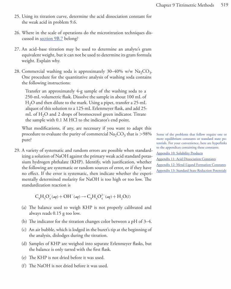
519Chapter 9 Titrimetric Methods
25. Using its titration curve, determine the acid dissociation constant for the weak acid in problem 9.6.
26. Where in the scale of operations do the microtitration techniques dis-cussed in section 9B.7 belong?
27. An acid–base titration may be used to determine an analyte’s gram equivalent weight, but it can not be used to determine its gram formula weight. Explain why.
28. Commercial washing soda is approximately 30–40% w/w Na2CO3. One procedure for the quantitative analysis of washing soda contains the following instructions:
Transfer an approximately 4-g sample of the washing soda to a 250-mL volumetric flask. Dissolve the sample in about 100 mL of H2O and then dilute to the mark. Using a pipet, transfer a 25-mL aliquot of this solution to a 125-mL Erlenmeyer flask, and add 25-mL of H2O and 2 drops of bromocresol green indicator. Titrate the sample with 0.1 M HCl to the indicator’s end point.
What modifications, if any, are necessary if you want to adapt this procedure to evaluate the purity of commercial Na2CO3 that is >98% pure?
29. A variety of systematic and random errors are possible when standard-izing a solution of NaOH against the primary weak acid standard potas-sium hydrogen phthalate (KHP). Identify, with justification, whether the following are systematic or random sources of error, or if they have no effect. If the error is systematic, then indicate whether the experi-mentally determined molarity for NaOH is too high or too low. The standardization reaction is
C H O OH C H O H O8 5 8 4 24 42− − −+ → +( ) ( ) ( ) ( )aq aq aq l
(a) The balance used to weigh KHP is not properly calibrated and always reads 0.15 g too low.
(b) The indicator for the titration changes color between a pH of 3–4.
(c) An air bubble, which is lodged in the buret’s tip at the beginning of the analysis, dislodges during the titration.
(d) Samples of KHP are weighed into separate Erlenmeyer flasks, but the balance is only tarred with the first flask.
(e) The KHP is not dried before it was used.
(f ) The NaOH is not dried before it was used.
Some of the problems that follow require one or more equilibrium constants or standard state po-tentials. For your convenience, here are hyperlinks to the appendices containing these constants
Appendix 10: Solubility Products
Appendix 11: Acid Dissociation Constants
Appendix 12: Metal-Ligand Formation Constants
Appendix 13: Standard State Reduction Potentials
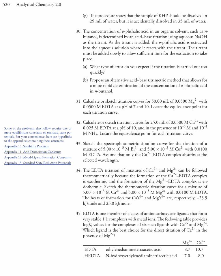
520 Analytical Chemistry 2.0
(g) The procedure states that the sample of KHP should be dissolved in 25 mL of water, but it is accidentally dissolved in 35 mL of water.
30. The concentration of o-phthalic acid in an organic solvent, such as n-butanol, is determined by an acid–base titration using aqueous NaOH as the titrant. As the titrant is added, the o-phthalic acid is extracted into the aqueous solution where it reacts with the titrant. The titrant must be added slowly to allow sufficient time for the extraction to take place.
(a) What type of error do you expect if the titration is carried out too quickly?
(b) Propose an alternative acid–base titrimetric method that allows for a more rapid determination of the concentration of o-phthalic acid in n-butanol.
31. Calculate or sketch titration curves for 50.00 mL of 0.0500 Mg2+ with 0.0500 M EDTA at a pH of 7 and 10. Locate the equivalence point for each titration curve.
32. Calculate or sketch titration curves for 25.0 mL of 0.0500 M Cu2+ with 0.025 M EDTA at a pH of 10, and in the presence of 10–3 M and 10–1 M NH3. Locate the equivalence point for each titration curve.
33. Sketch the spectrophotometric titration curve for the titration of a mixture of 5.00 � 10–3 M Bi3+ and 5.00 � 10–3 M Cu2+ with 0.0100 M EDTA. Assume that only the Cu2+–EDTA complex absorbs at the selected wavelength.
34. The EDTA titration of mixtures of Ca2+ and Mg2+ can be followed thermometrically because the formation of the Ca2+–EDTA complex is exothermic and the formation of the Mg2+–EDTA complex is en-dothermic. Sketch the thermometric titration curve for a mixture of 5.00 � 10–3 M Ca2+ and 5.00 � 10–3 M Mg2+ with 0.0100 M EDTA. The heats of formation for CaY2– and MgY2– are, respectively, –23.9 kJ/mole and 23.0 kJ/mole.
35. EDTA is one member of a class of aminocarboxylate ligands that form very stable 1:1 complexes with metal ions. The following table provides logKf values for the complexes of six such ligands with Ca2+ and Mg2+. Which ligand is the best choice for the direct titration of Ca2+ in the presence of Mg2+?
Mg2+ Ca2+
EDTA ethylenediaminetetraacetic acid 8.7 10.7HEDTA N-hydroxyethylenediaminetriacetic acid 7.0 8.0
Some of the problems that follow require one or more equilibrium constants or standard state po-tentials. For your convenience, here are hyperlinks to the appendices containing these constants
Appendix 10: Solubility Products
Appendix 11: Acid Dissociation Constants
Appendix 12: Metal-Ligand Formation Constants
Appendix 13: Standard State Reduction Potentials

521Chapter 9 Titrimetric Methods
Mg2+ Ca2+
EEDTA ethyletherdiaminetetraacetic acid 8.3 10.0DGTA ethyleneglycol-bis(b-aminoethylether)-
N,N´-tetraacetic acid5.4 10.9
DTPA diethylenetriaminepentaacetic acid 9.0 10.7CyDTA cyclohexanediaminetetraacetic acid 10.3 12.3
36. The amount of calcium in physiological fluids can be determined by a complexometric titration with EDTA. In one such analysis a 0.100-mL sample of a blood serum was made basic by adding 2 drops of NaOH and titrated with 0.00119 M EDTA, requiring 0.268 mL to reach the end point. Report the concentration of calcium in the sample as mil-ligrams Ca per 100 mL.
37. After removing the membranes from an eggshell, the shell is dried and its mass recorded as 5.613 g. The eggshell is transferred to a 250-mL beaker and dissolved in 25 mL of 6 M HCl. After filtering, the solution containing the dissolved eggshell is diluted to 250 mL in a volumetric flask. A 10.00-mL aliquot is placed in a 125-mL Erlenmeyer flask and buffered to a pH of 10. Titrating with 0.04988 M EDTA requires 44.11 mL to reach the end point. Determine the amount of calcium in the eggshell as %w/w CaCO3.
38. The concentration of cyanide, CN–, in a copper electroplating bath can be determined by a complexometric titration with Ag+, forming the soluble Ag(CN)2
– complex. In a typical analysis a 5.00-mL sample from an electroplating bath is transferred to a 250-mL Erlenmeyer flask, and treated with 100 mL of H2O, 5 mL of 20% w/v NaOH and 5 mL of 10% w/v KI. The sample is titrated with 0.1012 M AgNO3, requir-ing 27.36 mL to reach the end point as signaled by the formation of a yellow precipitate of AgI. Report the concentration of cyanide as parts per million of NaCN.
39. Before the introduction of EDTA most complexation titrations used Ag+ or CN– as the titrant. The analysis for Cd2+, for example, was ac-complished indirectly by adding an excess of KCN to form Cd(CN)4
2–, and back titrating the excess CN– with Ag+, forming Ag(CN)2
–. In one such analysis a 0.3000-g sample of an ore was dissolved and treated with 20.00 mL of 0.5000 M KCN. The excess CN– required 13.98 mL of 0.1518 M AgNO3 to reach the end point. Determine the %w/w Cd in the ore.
40. Solutions containing both Fe3+ and Al3+ can be selectively analyzed for Fe3+ by buffering to a pH of 2 and titrating with EDTA. The pH of the solution is then raised to 5 and an excess of EDTA added, resulting in
Some of the problems that follow require one or more equilibrium constants or standard state po-tentials. For your convenience, here are hyperlinks to the appendices containing these constants
Appendix 10: Solubility Products
Appendix 11: Acid Dissociation Constants
Appendix 12: Metal-Ligand Formation Constants
Appendix 13: Standard State Reduction Potentials

522 Analytical Chemistry 2.0
the formation of the Al3+–EDTA complex. The excess EDTA is back-titrated using a standard solution of Fe3+, providing an indirect analysis for Al3+.
(a) At a pH of 2, verify that the formation of the Fe3+–EDTA complex is favorable, and that the formation of the Al3+–EDTA complex is not favorable.
(b) A 50.00-mL aliquot of a sample containing Fe3+ and Al3+ is trans-ferred to a 250-mL Erlenmeyer flask and buffered to a pH of 2. A small amount of salicylic acid is added, forming the soluble red-colored Fe3+–salicylic acid complex. The solution is titrated with 0.05002 M EDTA, requiring 24.82 mL to reach the end point as signaled by the disappearance of the Fe3+–salicylic acid complex’s red color. The solution is buffered to a pH of 5 and 50.00 mL of 0.05002 M EDTA is added. After ensuring that the formation of the Al3+–EDTA complex is complete, the excess EDTA was back titrated with 0.04109 M Fe3+, requiring 17.84 mL to reach the end point as signaled by the reappearance of the red-colored Fe3+–salicylic acid complex. Report the molar concentrations of Fe3+ and Al3+ in the sample.
41. Prada and colleagues described an indirect method for determining sulfate in natural samples, such as seawater and industrial effluents.12 The method consists of three steps: precipitating the sulfate as PbSO4; dissolving the PbSO4 in an ammonical solution of excess EDTA to form the soluble PbY2– complex; and titrating the excess EDTA with a standard solution of Mg2+. The following reactions and equilibrium constants are known
PbSO Pb SO42
42( ) ( ) ( )s aq aq
+ −+ Ksp = 1.6 � 10–8
Pb Y PbY2 4 2+ − −+( ) ( ) ( )aq aq aq Kf = 1.1 � 1018
Mg Y MgY2 4 2+ − −+( ) ( ) ( )aq aq aq Kf = 4.9 � 108
Zn Y ZnY2 4 2+ − −+( ) ( ) ( )aq aq aq Kf = 3.2 � 1016
(a) Verify that a precipitate of PbSO4 dissolves in a solution of Y4–.
(b) Sporek proposed a similar method using Zn2+ as a titrant and found that the accuracy was frequently poor.13 One explanation is that Zn2+ might react with the PbY2– complex, forming ZnY2–. Show that this might be a problem when using Zn2+ as a titrant, but that it is not a problem when using Mg2+ as a titrant. Would such a
12 Prada, S.; Guekezian, M.; Suarez-Iha, M. E. V. Anal. Chim. Acta 1996, 329, 197–202.13 Sporek, K. F. Anal. Chem. 1958, 30, 1030–1032.
Some of the problems that follow require one or more equilibrium constants or standard state po-tentials. For your convenience, here are hyperlinks to the appendices containing these constants
Appendix 10: Solubility Products
Appendix 11: Acid Dissociation Constants
Appendix 12: Metal-Ligand Formation Constants
Appendix 13: Standard State Reduction Potentials

523Chapter 9 Titrimetric Methods
displacement of Pb2+ by Zn2+ lead to the reporting of too much or too little sulfate?
(c) In a typical analysis, a 25.00-mL sample of an industrial effluent was carried through the procedure using 50.00 mL of 0.05000 M EDTA. Titrating the excess EDTA required 12.42 mL of 0.1000 M Mg2+. Report the molar concentration of SO4
2– in the sample of effluent.
42. Table 9.10 provides values for the fraction of EDTA present as Y4-, aY4–. Values of aY4– are calculated using the equation
αY
EDTA
Y4
4
− =−[ ]
C
where [Y4-] is the concentration of the fully deprotonated EDTA and CEDTA is the total concentration of EDTA in all of its forms
CEDTA 6 5 4
3 2
H Y H Y H Y
H Y H Y
= + + +
+ +
+ +
− −
[ ] [ ] [ ]
[ ] [ ] [
2
2 HHY Y3 4− −+] [ ]
Using the following equilibria
H Y H O H O H Y6 2 3 52+ + ++ +( ) ( ) ( ) ( )aq l aq aq Ka1
H Y H O H O H Y5 2 3 4+ ++ +( ) ( ) ( ) ( )aq l aq aq Ka2
H Y H O H O H Y4 2 3 3( ) ( ) ( ) ( )aq l aq aq+ ++ − Ka3
H Y H O H O H Y3 2 3 2− + −+ +( ) ( ) ( ) ( )aq l aq aq
2 Ka4
H Y H O H O HY2 2 32 3− + −+ +( ) ( ) ( ) ( )aq l aq aq Ka5
HY H O H O Y2 33 4− + −+ +( ) ( ) ( ) ( )aq l aq aq Ka6
show that
αY
K K K K K Kd4− =
a1 a2 a3 a4 a5 a6
where
d K K K
K K K
= + + ++ + +
+
[ ] [ ] [ ]
[ ]
H H H
Ha1 a1 a2
a1 a2 a3
6 5 4
3 ++ +
+
+
+
[ ]
[ ]
H
Ha1 a2 a3 a4
a1 a2 a3 a4 a5 a
2
1
K K K K
K K K K K K 11 a2 a3 a4 a5 a6K K K K K
Some of the problems that follow require one or more equilibrium constants or standard state po-tentials. For your convenience, here are hyperlinks to the appendices containing these constants
Appendix 10: Solubility Products
Appendix 11: Acid Dissociation Constants
Appendix 12: Metal-Ligand Formation Constants
Appendix 13: Standard State Reduction Potentials

524 Analytical Chemistry 2.0
43. Calculate or sketch titration curves for the following (unbalanced) re-dox titration reactions at 25 oC. Assume the analyte is initially present at a concentration of 0.0100 M and that a 25.0-mL sample is taken for analysis. The titrant, which is the underlined species in each reaction, is 0.0100 M.
(a) V Ce V Ce2 4 3 3+ + + ++ → +( ) ( ) ( ) ( )aq aq aq aq
(b) Ti Fe Ti Fe2 3 3 2+ + + ++ → +( ) ( ) ( ) ( )aq aq aq aq
(c) Fe MnO Fe Mn4 (at pH2 3 2+ − + ++ → +( ) ( ) ( ) ( )aq aq aq aq == 1)
44. What is the equivalence point for each titration in problem 43?
45. Suggest an appropriate indicator for each titration in problem 43.
46. The iron content of an ore can be determined by a redox titration using K2Cr2O7 as the titrant. A sample of the ore is dissolved in concentrated HCl using Sn2+ to speed its dissolution by reducing Fe3+ to Fe2+. After the sample is dissolved, Fe2+ and any excess Sn2+ are oxidized to Fe3+
and Sn4+ using MnO4–. The iron is then carefully reduced to Fe2+ by
adding a 2–3 drop excess of Sn2+. A solution of HgCl2 is added and, if a white precipitate of Hg2Cl2 forms, the analysis is continued by titrat-ing with K2Cr2O7. The sample is discarded without completing the analysis if a precipitate of Hg2Cl2 does not form, or if a gray precipitate (due to Hg) forms.
(a) Explain why the analysis is not completed if a white precipitate of Hg2Cl2 forms, or if a gray precipitate forms.
(b) Is a determinate error introduced if the analyst forgets to add Sn2+ in the step where the iron ore is dissolved?
(c) Is a determinate error introduced if the iron is not quantitatively oxidized back to Fe3+ by the MnO4
–?
47. The amount of Cr3+ in an inorganic salt can be determined by a redox titration. A portion of sample containing approximately 0.25 g of Cr3+
is accurately weighed and dissolved in 50 mL of H2O. The Cr3+ is oxidized to Cr2O7
2– by adding 20 mL of 0.1 M AgNO3, which serves as a catalyst, and 50 mL of 10%w/v (NH4)2S2O8, which serves as the oxidizing agent. After the reaction is complete the resulting solution is boiled for 20 minutes to destroy the excess S2O8
2–, cooled to room temperature, and diluted to 250 mL in a volumetric flask. A 50-mL portion of the resulting solution is transferred to an Erlenmeyer flask, treated with 50 mL of a standard solution of Fe2+, and acidified with 200 mL of 1 M H2SO4, reducing the Cr2O7
2– to Cr3+. The excess Fe2+ is then determined by a back titration with a standard solution
Some of the problems that follow require one or more equilibrium constants or standard state po-tentials. For your convenience, here are hyperlinks to the appendices containing these constants
Appendix 10: Solubility Products
Appendix 11: Acid Dissociation Constants
Appendix 12: Metal-Ligand Formation Constants
Appendix 13: Standard State Reduction Potentials

525Chapter 9 Titrimetric Methods
of K2Cr2O7 using an appropriate indicator. The results are reported as %w/w Cr3+.
(a) There are several places in the procedure where a reagent’s volume is specified (see underlined text). Which of these measurements must be made using a volumetric pipet.
(b) Excess peroxydisulfate, S2O82– is destroyed by boiling the solution.
What is the effect on the reported %w/w Cr3+ if some of the S2O82–
is not destroyed during this step?
(c) Solutions of Fe2+ undergo slow air oxidation to Fe3+. What is the effect on the reported %w/w Cr3+ if the standard solution of Fe2+ is inadvertently allowed to be partially oxidized?
48. The exact concentration of H2O2 in a solution that is nominally 6% w/v H2O2 can be determined by a redox titration with MnO4
–. A 25-mL aliquot of the sample is transferred to a 250-mL volumetric flask and diluted to volume with distilled water. A 25-mL aliquot of the diluted sample is added to an Erlenmeyer flask, diluted with 200 mL of distilled water, and acidified with 20 mL of 25% v/v H2SO4. The resulting solution is titrated with a standard solution of KMnO4 until a faint pink color persists for 30 s. The results are reported as %w/v H2O2.
(a) Many commercially available solutions of H2O2 contain an inor-ganic or organic stabilizer to prevent the autodecomposition of the peroxide to H2O and O2. What effect does the presence of this stabilizer have on the reported %w/v H2O2 if it also reacts with MnO4
–?
(b) Laboratory distilled water often contains traces of dissolved organic material that may react with MnO4
–. Describe a simple method to correct for this potential interference.
(c) What modifications to the procedure, if any, are need if the sample has a nominal concentration of 30% w/v H2O2.
49. The amount of iron in a meteorite was determined by a redox titration using KMnO4 as the titrant. A 0.4185-g sample was dissolved in acid and the liberated Fe3+ quantitatively reduced to Fe2+ using a Walden reductor. Titrating with 0.02500 M KMnO4 requires 41.27 mL to reach the end point. Determine the %w/w Fe2O3 in the sample of meteorite.
50. Under basic conditions, MnO4– can be used as a titrant for the analysis
of Mn2+, with both the analyte and the titrant forming MnO2. In the analysis of a mineral sample for manganese, a 0.5165-g sample is dis-solved and the manganese reduced to Mn2+. The solution is made basic
Some of the problems that follow require one or more equilibrium constants or standard state po-tentials. For your convenience, here are hyperlinks to the appendices containing these constants
Appendix 10: Solubility Products
Appendix 11: Acid Dissociation Constants
Appendix 12: Metal-Ligand Formation Constants
Appendix 13: Standard State Reduction Potentials
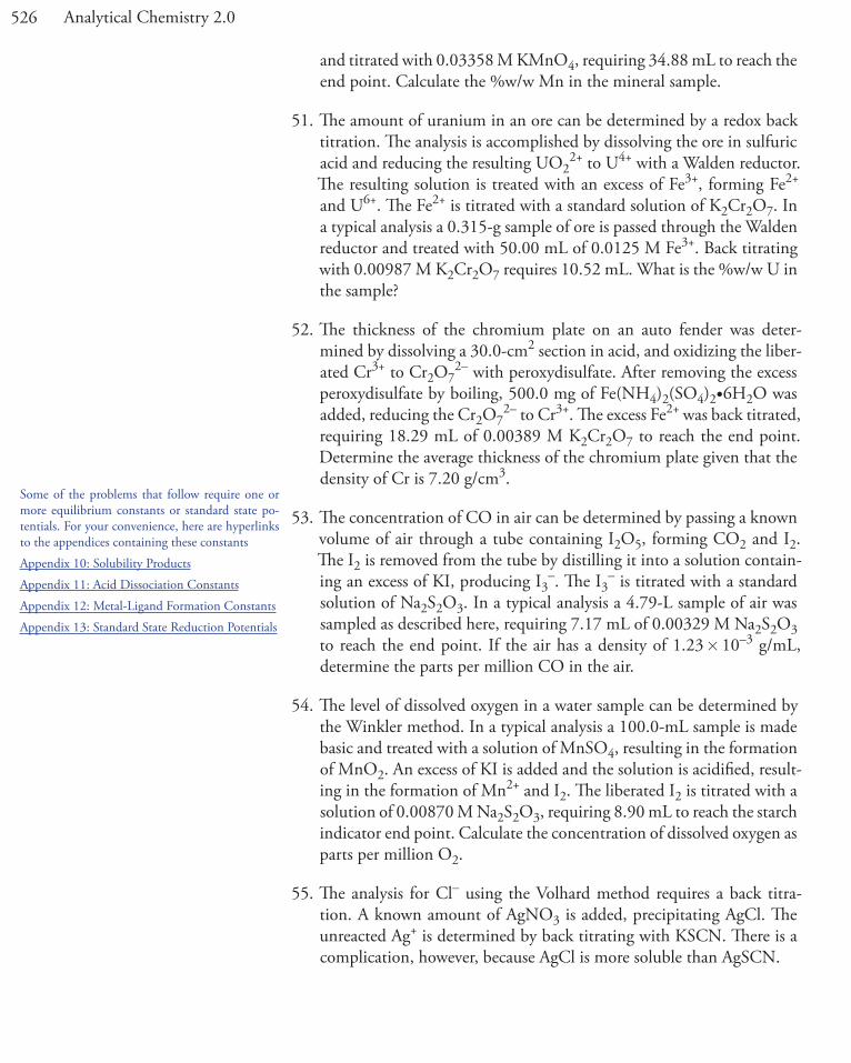
526 Analytical Chemistry 2.0
and titrated with 0.03358 M KMnO4, requiring 34.88 mL to reach the end point. Calculate the %w/w Mn in the mineral sample.
51. The amount of uranium in an ore can be determined by a redox back titration. The analysis is accomplished by dissolving the ore in sulfuric acid and reducing the resulting UO2
2+ to U4+ with a Walden reductor. The resulting solution is treated with an excess of Fe3+, forming Fe2+ and U6+. The Fe2+ is titrated with a standard solution of K2Cr2O7. In a typical analysis a 0.315-g sample of ore is passed through the Walden reductor and treated with 50.00 mL of 0.0125 M Fe3+. Back titrating with 0.00987 M K2Cr2O7 requires 10.52 mL. What is the %w/w U in the sample?
52. The thickness of the chromium plate on an auto fender was deter-mined by dissolving a 30.0-cm2 section in acid, and oxidizing the liber-ated Cr3+ to Cr2O7
2– with peroxydisulfate. After removing the excess peroxydisulfate by boiling, 500.0 mg of Fe(NH4)2(SO4)2•6H2O was added, reducing the Cr2O7
2– to Cr3+. The excess Fe2+ was back titrated, requiring 18.29 mL of 0.00389 M K2Cr2O7 to reach the end point. Determine the average thickness of the chromium plate given that the density of Cr is 7.20 g/cm3.
53. The concentration of CO in air can be determined by passing a known volume of air through a tube containing I2O5, forming CO2 and I2. The I2 is removed from the tube by distilling it into a solution contain-ing an excess of KI, producing I3
–. The I3– is titrated with a standard
solution of Na2S2O3. In a typical analysis a 4.79-L sample of air was sampled as described here, requiring 7.17 mL of 0.00329 M Na2S2O3 to reach the end point. If the air has a density of 1.23 � 10–3 g/mL, determine the parts per million CO in the air.
54. The level of dissolved oxygen in a water sample can be determined by the Winkler method. In a typical analysis a 100.0-mL sample is made basic and treated with a solution of MnSO4, resulting in the formation of MnO2. An excess of KI is added and the solution is acidified, result-ing in the formation of Mn2+ and I2. The liberated I2 is titrated with a solution of 0.00870 M Na2S2O3, requiring 8.90 mL to reach the starch indicator end point. Calculate the concentration of dissolved oxygen as parts per million O2.
55. The analysis for Cl– using the Volhard method requires a back titra-tion. A known amount of AgNO3 is added, precipitating AgCl. The unreacted Ag+ is determined by back titrating with KSCN. There is a complication, however, because AgCl is more soluble than AgSCN.
Some of the problems that follow require one or more equilibrium constants or standard state po-tentials. For your convenience, here are hyperlinks to the appendices containing these constants
Appendix 10: Solubility Products
Appendix 11: Acid Dissociation Constants
Appendix 12: Metal-Ligand Formation Constants
Appendix 13: Standard State Reduction Potentials
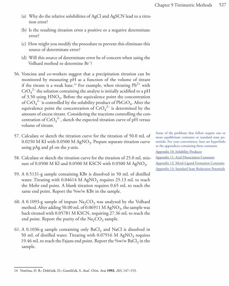
527Chapter 9 Titrimetric Methods
(a) Why do the relative solubilities of AgCl and AgSCN lead to a titra-tion error?
(b) Is the resulting titration error a positive or a negative determinate error?
(c) How might you modify the procedure to prevent this eliminate this source of determinate error?
(d) Will this source of determinate error be of concern when using the Volhard method to determine Br–?
56. Voncina and co-workers suggest that a precipitation titration can be monitored by measuring pH as a function of the volume of titrant if the titrant is a weak base.14 For example, when titrating Pb2+ with CrO4
2– the solution containing the analyte is initially acidified to a pH of 3.50 using HNO3. Before the equivalence point the concentration of CrO4
2– is controlled by the solubility product of PbCrO4. After the equivalence point the concentration of CrO4
2– is determined by the amount of excess titrant. Considering the reactions controlling the con-centration of CrO4
2–, sketch the expected titration curve of pH versus volume of titrant.
57. Calculate or sketch the titration curve for the titration of 50.0 mL of 0.0250 M KI with 0.0500 M AgNO3. Prepare separate titration curve using pAg and pI on the y-axis.
58. Calculate or sketch the titration curve for the titration of 25.0 mL mix-ture of 0.0500 M KI and 0.0500 M KSCN with 0.0500 M AgNO3.
59. A 0.5131-g sample containing KBr is dissolved in 50 mL of distilled water. Titrating with 0.04614 M AgNO3 requires 25.13 mL to reach the Mohr end point. A blank titration requires 0.65 mL to reach the same end point. Report the %w/w KBr in the sample.
60. A 0.1093-g sample of impure Na2CO3 was analyzed by the Volhard method. After adding 50.00 mL of 0.06911 M AgNO3, the sample was back titrated with 0.05781 M KSCN, requiring 27.36 mL to reach the end point. Report the purity of the Na2CO3 sample.
61. A 0.1036-g sample containing only BaCl2 and NaCl is dissolved in 50 mL of distilled water. Titrating with 0.07916 M AgNO3 requires 19.46 mL to reach the Fajans end point. Report the %w/w BaCl2 in the sample.
14 VonČina, D. B.; DobČnik, D.; GomiŠČek, S. Anal. Chim. Acta 1992, 263, 147–153.
Some of the problems that follow require one or more equilibrium constants or standard state po-tentials. For your convenience, here are hyperlinks to the appendices containing these constants
Appendix 10: Solubility Products
Appendix 11: Acid Dissociation Constants
Appendix 12: Metal-Ligand Formation Constants
Appendix 13: Standard State Reduction Potentials

528 Analytical Chemistry 2.0
9I Solutions to Practice ExercisesPractice Exercise 9.1The volume of HCl needed to reach the equivalence point is
V VM VMeq a
b b
a
M)(25.0 mL)M
= = = =( .
.0 125
0 062550..0 mL
Before the equivalence point, NaOH is present in excess and the pH is determined by the concentration of unreacted OH–. For example, after adding 10.0 mL of HCl
[ ]( . (
OHM)(25.0 mL) 0.0625 M)(10.0 mL− =
−0 125 ))25.0 mL 10.0 mL
M+
= 0 0714.
[ ][ ]
..
.H OOH M3
w+−
−−= =
�= �
K 1 00 100 0714
1 40 1014
133 M
the pH is 12.85.
For the titration of a strong base with a strong acid the pH at the equiva-lence point is 7.00.
For volumes of HCl greater than the equivalence point, the pH is deter-mined by the concentration of excess HCl. For example, after adding 70.0 mL of titrant the concentration of HCl is
[ ]( . (
HClM)(70.0 mL) 0.125 M)(25.0 mL
=−0 0625 ))
70.0 mL 25.0 mLM
+= 0 0132.
giving a pH of 1.88. Some additional results are shown here.Volume of HCl (mL) pH Volume of HCl (mL) pH
0 13.10 60 2.1310 12.85 70 1.8820 12.62 80 1.7530 12.36 90 1.6640 11.98 100 1.6050 7.00
Click here to return to the chapter.
Practice Exercise 9.2The volume of HCl needed to reach the equivalence point is
V VM VMeq a
b b
a
M)(25.0 mL)M
= = = =( .
.0 125
0 062550..0 mL
Before adding HCl the pH is that for a solution of 0.100 M NH3.

529Chapter 9 Titrimetric Methods
Kx x
xb4
3
OH NHNH 0.125
= =−
= �− +
−[ ][ ][ ]
( )( ).1 75 10 5
x = = �− −[ ] .OH M1 47 10 3
The pH at the beginning of the titration, therefore, is 11.17.
Before the equivalence point the pH is determined by an NH3/NH4+
buffer. For example, after adding 10.0 mL of HCl
[ ]NH(0.125 M)(25.0 mL) (0.0625 M)(10.0 mL
3 =− ))
25.0 mL mLM
+=
10 00 0714
..
[ ]( .
.NH
M)(10.0 mL)25.0 mL mL4
+ =+
=0 0625
10 000 0179. M
pHMM
= + =9 2440 07140 0179
9 84. log..
.
At the equivalence point the predominate ion in solution is NH4+. To
calculate the pH we first determine the concentration of NH4+
[ ]( .
.NH
M)(25.0 mL)25.0 mL mL4
+ =+
=0 125
50 00..0417 M
and then calculate the pH
Kx x
xa3 3
4
H O NHNH 0.0417
= =−
= �+
+
[ ][ ][ ]
( )( ).5 70 10−−10
x = = �+ −[ ] .H O M3 4 88 10 6
obtaining a value of 5.31.
After the equivalence point, the pH is determined by the excess HCl. For example, after adding 70.0 mL of HCl
[ ]( . (
HClM)(70.0 mL) 0.125 M)(25.0 mL
=−0 0625 ))
25.0 mL 70.0 mLM
+= 0 0132.
and the pH is 1.88. Some additional results are shown here.Volume of HCl (mL) pH Volume of HCl (mL) pH
0 11.17 60 2.1310 9.84 70 1.8820 9.42 80 1.7530 9.07 90 1.6640 8.64 100 1.6050 5.31
Click here to return to the chapter.
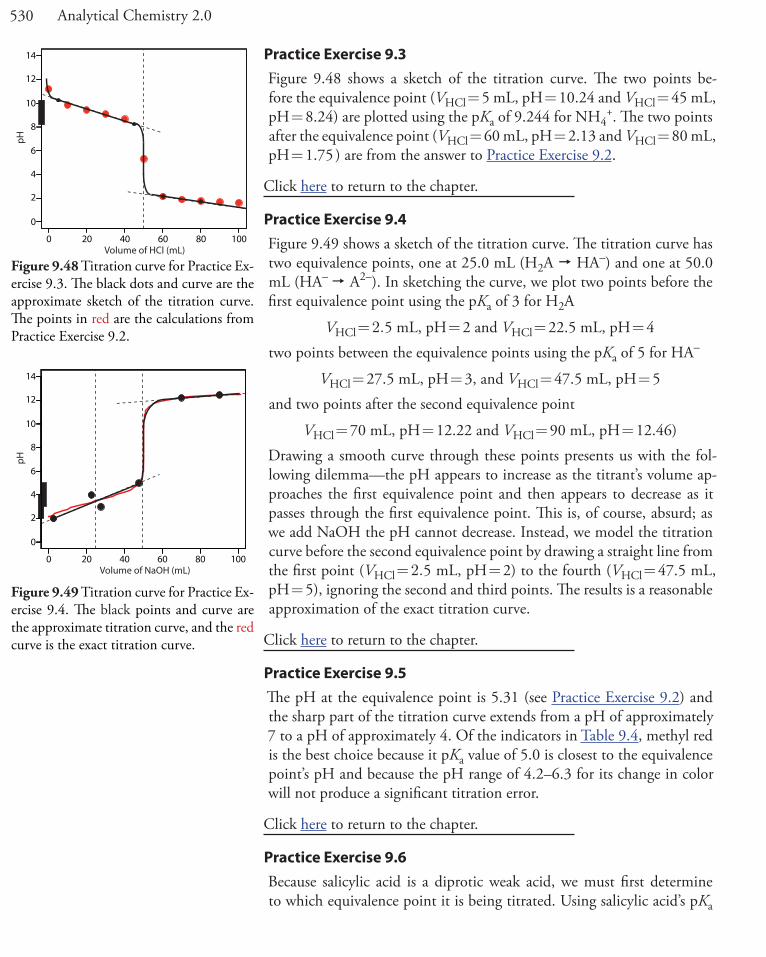
530 Analytical Chemistry 2.0
Practice Exercise 9.3Figure 9.48 shows a sketch of the titration curve. The two points be-fore the equivalence point (VHCl = 5 mL, pH = 10.24 and VHCl = 45 mL, pH = 8.24) are plotted using the pKa of 9.244 for NH4
+. The two points after the equivalence point (VHCl = 60 mL, pH = 2.13 and VHCl = 80 mL, pH = 1.75 ) are from the answer to Practice Exercise 9.2.
Click here to return to the chapter.
Practice Exercise 9.4Figure 9.49 shows a sketch of the titration curve. The titration curve has two equivalence points, one at 25.0 mL (H2A HA–) and one at 50.0 mL (HA– A2–). In sketching the curve, we plot two points before the first equivalence point using the pKa of 3 for H2A
VHCl = 2.5 mL, pH = 2 and VHCl = 22.5 mL, pH = 4two points between the equivalence points using the pKa of 5 for HA–
VHCl = 27.5 mL, pH = 3, and VHCl = 47.5 mL, pH = 5and two points after the second equivalence point
VHCl = 70 mL, pH = 12.22 and VHCl = 90 mL, pH = 12.46)Drawing a smooth curve through these points presents us with the fol-lowing dilemma—the pH appears to increase as the titrant’s volume ap-proaches the first equivalence point and then appears to decrease as it passes through the first equivalence point. This is, of course, absurd; as we add NaOH the pH cannot decrease. Instead, we model the titration curve before the second equivalence point by drawing a straight line from the first point (VHCl = 2.5 mL, pH = 2) to the fourth (VHCl = 47.5 mL, pH = 5), ignoring the second and third points. The results is a reasonable approximation of the exact titration curve.
Click here to return to the chapter.
Practice Exercise 9.5The pH at the equivalence point is 5.31 (see Practice Exercise 9.2) and the sharp part of the titration curve extends from a pH of approximately 7 to a pH of approximately 4. Of the indicators in Table 9.4, methyl red is the best choice because it pKa value of 5.0 is closest to the equivalence point’s pH and because the pH range of 4.2–6.3 for its change in color will not produce a significant titration error.
Click here to return to the chapter.
Practice Exercise 9.6Because salicylic acid is a diprotic weak acid, we must first determine to which equivalence point it is being titrated. Using salicylic acid’s pKa
Figure 9.48 Titration curve for Practice Ex-ercise 9.3. The black dots and curve are the approximate sketch of the titration curve. The points in red are the calculations from Practice Exercise 9.2.
Figure 9.49 Titration curve for Practice Ex-ercise 9.4. The black points and curve are the approximate titration curve, and the red curve is the exact titration curve.
0 20 40 60 80 100
0
2
4
6
8
10
12
14
pH
Volume of HCl (mL)
0 20 40 60 80 100
0
2
4
6
8
10
12
14
pH
Volume of NaOH (mL)

531Chapter 9 Titrimetric Methods
values as a guide, the pH at the first equivalence point is between a pH of 2.97 and 13.74, and the second equivalence points is at a pH greater than 13.74. From Table 9.4, phenolphthalein’s end point falls in the pH range 8.3–10.0. The titration, therefore, is to the first equivalence point for which the moles of NaOH equal the moles of salicylic acid; thus
0 13540 02192 2 968 10 3.. .
mol NaOHL
L mol N� = � − aaOH
2 968 101
13
3. � � �− mol NaOHmol C H Omol NaOH
7 6 3
88 120 4099
..
g C H Omol C H O
g C H O7 6 3
7 6 37 6 3=
0 40990 4208
100 97 41..
. %g C H Og sample
w7 6 3� = //w C H O7 6 3
Because the purity of the sample is less than 99%, we reject the ship-ment.
Click here to return to the chapter.
Practice Exercise 9.7The moles of HNO3 produced by pulling the air sample through the solution of H2O2 is
0 010120 00914
1
..
mol NaOHL
L
mol HNOmol N
3
� �
aaOHmol HNO3= � −9 25 10 5.
A conservation of mass on nitrogen requires that each mole of NO2 in the sample of air produces one mole of HNO3; thus, the mass of NO2 in the sample is
9 25 101
46 01
5.
.
� � �− mol HNOmol NO
mol HNO32
3
gg NOmol NO
g NO2
22= � −4 26 10 3.
and the concentration of NO2 is
4 26 105
10000 852
3..
�� =
− g NOL air
mgg
mg NO222 /L air
Click here to return to the chapter.
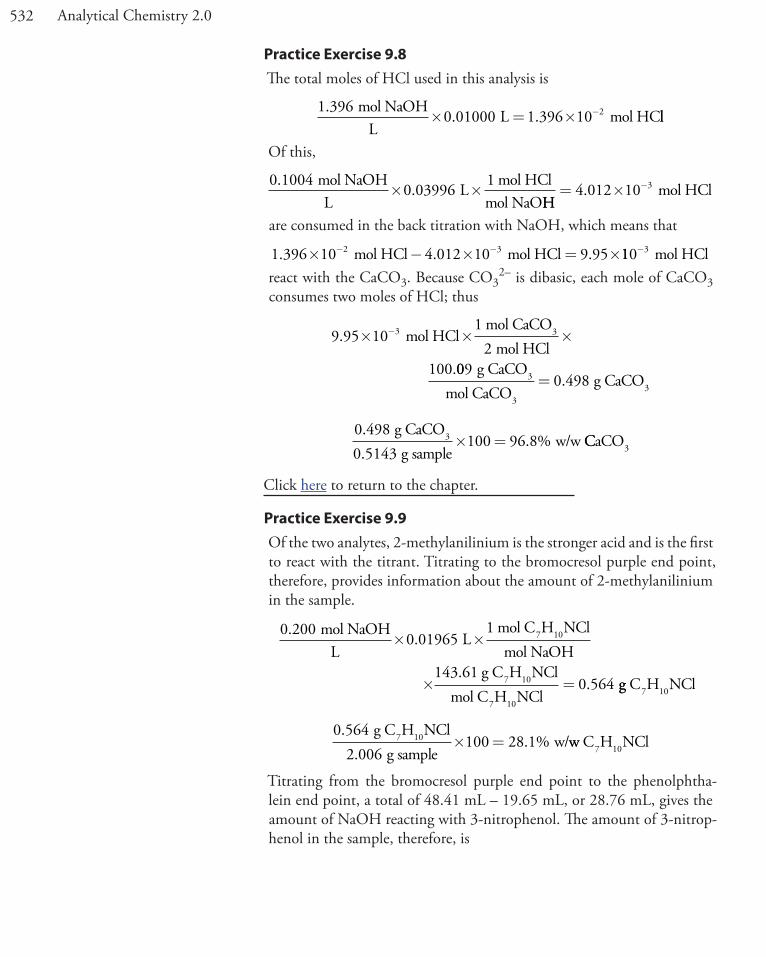
532 Analytical Chemistry 2.0
Practice Exercise 9.8The total moles of HCl used in this analysis is
1 3960 01000 1 396 10 2.. .
mol NaOHL
L mol HC� = � − ll
Of this,
0 10040 03996
1..
mol NaOHL
Lmol HCl
mol NaO� �
HHmol HCl= � −4 012 10 3.
are consumed in the back titration with NaOH, which means that
1 396 10 4 012 10 9 952 3. . .� − � = �− −mol HCl mol HCl 110 3− mol HClreact with the CaCO3. Because CO3
2– is dibasic, each mole of CaCO3 consumes two moles of HCl; thus
9 95 101
100
3.
.
� � �− mol HClmol CaCO2 mol HCl
3
0090 498
g CaCOmol CaCO
g CaCO3
33= .
0 4980 5143
100 96 8..
. %g CaCOg sample
w/w3 � = CCaCO3
Click here to return to the chapter.
Practice Exercise 9.9Of the two analytes, 2-methylanilinium is the stronger acid and is the first to react with the titrant. Titrating to the bromocresol purple end point, therefore, provides information about the amount of 2-methylanilinium in the sample.
0 2000 01965
1..
mol NaOHL
Lmol C H NClmol
7 10� �NaOH
g C H NClmol C H NCl
7 10
7 10
� =143 61
0 564.
. gg C H NCl7 10
0 5642 006
100 28 1.
.. %
g C H NClg sample
w/7 10 � = ww C H NCl7 10
Titrating from the bromocresol purple end point to the phenolphtha-lein end point, a total of 48.41 mL – 19.65 mL, or 28.76 mL, gives the amount of NaOH reacting with 3-nitrophenol. The amount of 3-nitrop-henol in the sample, therefore, is
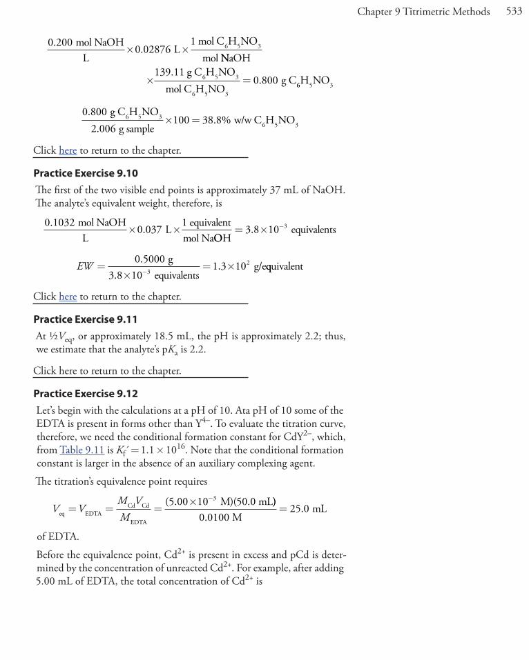
533Chapter 9 Titrimetric Methods
0 2000 02876
1..
mol NaOHL
Lmol C H NOmol
6 5 3� �NNaOH
g C H NOmol C H NO
g C6 5 3
6 5 3
� =139 11
0 800.
. 66 5 3H NO
0 8002 006
100 38 8.
.. %
g C H NOg sample
w/w6 5 3� = C H NO6 5 3
Click here to return to the chapter.
Practice Exercise 9.10The first of the two visible end points is approximately 37 mL of NaOH. The analyte’s equivalent weight, therefore, is
0 10320 037
1..
mol NaOHL
Lequivalent
mol Na� �
OOHequivalents= � −3 8 10 3.
EW =�
= �−
0 50003 8 10
1 3 103
2..
.g
equivalentsg/eqquivalent
Click here to return to the chapter.
Practice Exercise 9.11At ½Veq, or approximately 18.5 mL, the pH is approximately 2.2; thus, we estimate that the analyte’s pKa is 2.2.
Click here to return to the chapter.
Practice Exercise 9.12Let’s begin with the calculations at a pH of 10. Ata pH of 10 some of the EDTA is present in forms other than Y4–. To evaluate the titration curve, therefore, we need the conditional formation constant for CdY2–, which, from Table 9.11 is Kf´ = 1.1 � 1016. Note that the conditional formation constant is larger in the absence of an auxiliary complexing agent.
The titration’s equivalence point requires
V VM VMeq EDTA
Cd Cd
EDTA
M)(50.0 mL= = =
� −( .5 00 10 3 ))0.0100 M
mL= 25 0.
of EDTA.
Before the equivalence point, Cd2+ is present in excess and pCd is deter-mined by the concentration of unreacted Cd2+. For example, after adding 5.00 mL of EDTA, the total concentration of Cd2+ is

534 Analytical Chemistry 2.0
[ ]( .
CdM)(50.0 mL) (0.0100 M)(5.2
35 00 10+−
=� − 000 mL)
50.0 mL mLM
+= � −
5 003 64 10 3
..
which gives a pCd of 2.43.
At the equivalence point all the Cd2+ initially in the titrand is now pres-ent as CdY2–. The concentration of Cd2+, therefore, is determined by the dissociation of the CdY2– complex. First, we calculate the concentration of CdY2–.
[ ]( .
. .CdY
M)(50.0 mL)mL
235 00 10
50 0 25 0−
−
=�
+ mLM= � −3 33 10 3.
Next, we solve for the concentration of Cd2+ in equilibrium with CdY2–.
KC
xx xf
EDTA
CdYCd
′ = =� −
=−
+
−[ ][ ]
.( )( )
.2
2
33 33 101 11 1016�
Solving gives [Cd2+] as 5.50 � 10–10 M, or a pCd of 9.26 at the equiva-lence point.
After the equivalence point, EDTA is in excess and the concentration of Cd2+ is determined by the dissociation of the CdY2– complex. First, we calculate the concentrations of CdY2– and of unreacted EDTA. For ex-ample, after adding 30.0 mL of EDTA
[ ]( .
. .CdY
M)(50.0 mL)mL
235 00 10
50 0 30 0−
−
=�
+ mLM= � −3 13 10 3.
CEDTA
M)(30.0 mL) (5.00 M)(50.=
− � −( .0 0100 10 3 00 mL)mL 30.0 mL
M50 0
6 25 10 4
..
+= � −
Substituting into the equation for the conditional formation constant and solving for [Cd2+] gives
3 13 106 25 10
1 1 103
2 416.
[ ]( ..
��
= �−
+ −
MCd M)
[Cd2+] as 4.55� 10–16 M, or a pCd of 15.34.
The calculations at a pH of 7 are identical, except the conditional forma-tion constant for CdY2– is 1.5 � 1013 instead of 1.1 � 1016. The following table summarizes results for these two titrations as well as the results from Table 9.13 for the titration of Cd2+ at a pH of 10 in the presence of 0.0100 M NH3 as an auxiliary complexing agent.
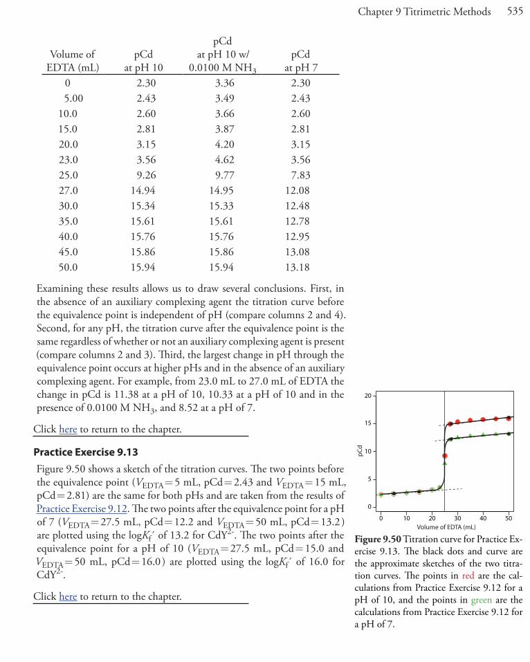
535Chapter 9 Titrimetric Methods
Volume of EDTA (mL)
pCd at pH 10
pCd at pH 10 w/
0.0100 M NH3
pCd at pH 7
0 2.30 3.36 2.305.00 2.43 3.49 2.43
10.0 2.60 3.66 2.6015.0 2.81 3.87 2.8120.0 3.15 4.20 3.1523.0 3.56 4.62 3.5625.0 9.26 9.77 7.8327.0 14.94 14.95 12.0830.0 15.34 15.33 12.4835.0 15.61 15.61 12.7840.0 15.76 15.76 12.9545.0 15.86 15.86 13.0850.0 15.94 15.94 13.18
Examining these results allows us to draw several conclusions. First, in the absence of an auxiliary complexing agent the titration curve before the equivalence point is independent of pH (compare columns 2 and 4). Second, for any pH, the titration curve after the equivalence point is the same regardless of whether or not an auxiliary complexing agent is present (compare columns 2 and 3). Third, the largest change in pH through the equivalence point occurs at higher pHs and in the absence of an auxiliary complexing agent. For example, from 23.0 mL to 27.0 mL of EDTA the change in pCd is 11.38 at a pH of 10, 10.33 at a pH of 10 and in the presence of 0.0100 M NH3, and 8.52 at a pH of 7.
Click here to return to the chapter.
Practice Exercise 9.13Figure 9.50 shows a sketch of the titration curves. The two points before the equivalence point (VEDTA = 5 mL, pCd = 2.43 and VEDTA = 15 mL, pCd = 2.81) are the same for both pHs and are taken from the results of Practice Exercise 9.12. The two points after the equivalence point for a pH of 7 (VEDTA = 27.5 mL, pCd = 12.2 and VEDTA = 50 mL, pCd = 13.2 ) are plotted using the logKf´ of 13.2 for CdY2-. The two points after the equivalence point for a pH of 10 (VEDTA = 27.5 mL, pCd = 15.0 and VEDTA = 50 mL, pCd = 16.0 ) are plotted using the logKf´ of 16.0 for CdY2-.
Click here to return to the chapter.
Figure 9.50 Titration curve for Practice Ex-ercise 9.13. The black dots and curve are the approximate sketches of the two titra-tion curves. The points in red are the cal-culations from Practice Exercise 9.12 for a pH of 10, and the points in green are the calculations from Practice Exercise 9.12 for a pH of 7.
0 10 20 30 40 50
0
5
10
15
20
Volume of EDTA (mL)
pCd

536 Analytical Chemistry 2.0
Practice Exercise 9.14In an analysis for hardness we treat the sample as if Ca2+ is the only metal ion reacting with EDTA. The grams of Ca2+ in the sample, therefore, is
0 01090 02363
1..
mol EDTAL
Lmol Ca
mol ED
2+
� �TTA
mol Ca2+= � −2 58 10 4.
2 58 101
100
4.
.
� � �− mol Camol CaCOmol Ca
2+ 32+
0090 0258
g CaCOmol CaCO
g CaCO3
33= .
and the sample’s hardness is
0 02580 1000
1000258
..
g CaCOL
mgg
mg CaCO3� = 33 /L
Click here to return to the chapter.
Practice Exercise 9.15The titration of CN– with Ag+ produces a metal-ligand complex of Ag(CN)2
2–; thus, each mole of AgNO3 reacts with two moles of NaCN. The grams of NaCN in the sample is
0 10180 03968
2..
mol AgNOL
Lmol NaCN
mol A3� �
ggNO
g NaCNmol NaCN
g NaCN
3
� =49 01
0 3959.
.
and the purity of the sample is
0 39590 4482
100 88 33..
. %g NaCNg sample
w/w� = NaCN
Click here to return to the chapter.
Practice Exercise 9.16The total moles of EDTA used in this analysis is
0.02011 mol EDTAL
L mol� = � −0 02500 5 028 10 4. . EEDTA
Of this,
0 011130 00423
1
..
mol MgL
L
mol EDTAmol M
2+
� �
ggmol EDTA
2+= � −4 708 10 5.
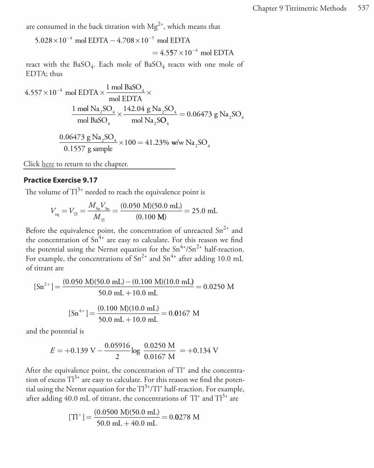
537Chapter 9 Titrimetric Methods
are consumed in the back titration with Mg2+, which means that
5 028 10 4 708 104 5
4 5. ..
� − �
=
− −mol EDTA mol EDTA557 10 4� − mol EDTA
react with the BaSO4. Each mole of BaSO4 reacts with one mole of EDTA; thus
4 557 101
1
4. � � �− mol EDTAmol BaSO
mol EDTAm
4
ool Na SOmol BaSO
g Na SOmol Na S
2 4
4
2 4
2
�142 04.
OOg Na SO
42 4= 0 06473.
0 064730 1557
100 41 23.
.. %
g Na SOg sample
2 4 � = ww/w Na SO2 4
Click here to return to the chapter.
Practice Exercise 9.17The volume of Tl3+ needed to reach the equivalence point is
V VM V
Meq TlSn Sn
Tl
M)(50.0 mL)(0.100
= = =( .0 050
MM)25.0 mL=
Before the equivalence point, the concentration of unreacted Sn2+ and the concentration of Sn4+ are easy to calculate. For this reason we find the potential using the Nernst equation for the Sn4+/Sn2+ half-reaction.For example, the concentrations of Sn2+ and Sn4+ after adding 10.0 mL of titrant are
[ ]( . ( .
SnM)(50.0 mL) M)(10.0 mL2 0 050 0 100+ =
− ))50.0 mL .0 mL
M+
=10
0 0250.
[ ]( .
.SnM)(10.0 mL)
50.0 mL .0 mL4 0 100
100+ =
+= 00167 M
and the potential is
E =+ −0 1390 05916
20 02500 0167
..
log..
VMM=+0 134. V
After the equivalence point, the concentration of Tl+ and the concentra-tion of excess Tl3+ are easy to calculate. For this reason we find the poten-tial using the Nernst equation for the Tl3+/Tl+ half-reaction. For example, after adding 40.0 mL of titrant, the concentrations of Tl+ and Tl3+ are
[ ]( .
..Tl
M)(50.0 mL)50.0 mL 0 mL
+ =+
=0 0500
400 00278 M

538 Analytical Chemistry 2.0
[ ]( . ( .
TlM)(40.0 mL) M)(50.0 m3 0 100 0 0500+ =
− LL)50.0 mL 40.0 mL
M+
= 0 0167.
and the potential is
E =+ −0 770 05916
20 02780 0167
..
log..
VMM=+0 76. V
At the titration’s equivalence point, the potential, Eeq, potential is
Eeq
V VV=
+=
0 139 0 772
0 45. .
.
Some additional results are shown here.Volume of Tl3+ (mL) E (V) Volume of Tl3+ (mL) E (V)
5 0.121 30 0.7510 0.134 35 0.7515 0.144 40 0.7620 0.157 45 0.7625 0.45 50 0.76
Click here to return to the chapter.
Practice Exercise 9.18Figure 9.51 shows a sketch of the titration curve. The two points before the equivalence point
VTl = 2.5 mL, E = +0.109 V and VTl = 22.5 mL, E = +0.169 V are plotted using the redox buffer for Sn4+/Sn2+, which spans a potential range of +0.139 ± 0.5916/2. The two points after the equivalence point
VTl= 27.5 mL, E = +0.74 V and VEDTA = 50 mL, E = +0.77 V are plotted using the redox buffer for Tl3+/Tl+, which spans the potential range of +0.139 ± 0.5916/2.
Click here to return to the chapter.
Practice Exercise 9.19The two half reactions are
Ce CeU H O UO4+
2
4 3
222
+ − +
+
+ →
+ → +
( ) ( )
( ) ( )
aq aq
aq aq
e
44 2H+ −+( )aq e
for which the Nernst equations are
E E= −+ +
+
+Ce Ceo Ce
Ce4 3
0 059161
3
4/
.log
[ ][ ]
Figure 9.51 Titration curve for Practice Ex-ercise 9.18. The black dots and curve are the approximate sketch of the titration curve. The points in red are the calculations from Practice Exercise 9.17.
0 10 20 30 40 50
0.0
0.2
0.4
0.6
0.8
Volume of Tl3+ (mL)
E (V
)

539Chapter 9 Titrimetric Methods
E E= −+ +
+
+ +UO Uo U
UO H22 4
0 059162
4
22 4/
.log
[ ][ ][ ]
Before adding these two equations together we must multiply the second equation by 2 so that we can combine the log terms; thus
3 2 0 059164 322 4
3
E E E= + −+ + + +
+
Ce Ceo
UO Uo Ce
/ /. log
[ ]][ ][ ][ ][ ]
UCe UO H
4
422 4
+
+ + +
At the equivalence point we know that
[ ] [ ]
[ ] [ ]
Ce UO
Ce U
322
4 4
2
2
+ +
+ +
= �
= �
Substituting these equalities into the previous equation and rearranging gives us a general equation for the potential at the equivalence point.
3 2 0 059162
4 322 4
2E E E= + −+ + + +Ce Ceo
UO Uo UO
/ /. log
[ 22 4
422 42
+ +
+ + +
][ ][ ][ ][ ]
UU UO H
EE E
=+
−+ + + +
+
Ce Ceo
UO Uo
H
4 322 42
30 05916
31/ / .
log[ ]]4
EE E
=+
+�+ + + +Ce Ce
oUO Uo
H4 3
22 42
30 05916 4
3/ / .
log[ ++ ]
EE E
=+
−+ + + +Ce Ce
oUO Uo
pH4 3
22 42
30 07888/ / .
At a pH of 1 the equivalence point has a potential of
Eeq V=+ �
− � =1 72 2 0 327
30 07888 1 0 712
. .. .
Click here to return to the chapter.
Practice Exercise 9.20Because we have not been provided with a balanced reaction, let’s use a conservation of electrons to deduce the stoichiometry. Oxidizing C2O4
2–, in which each carbon has a +3 oxidation state, to CO2, in which carbon has an oxidation state of +4, requires one electron per carbon, or a total of two electrons for each mole of C2O4
2–. Reducing MnO4–, in which each
manganese is in the +7 oxidation state, to Mn2+ requires five electrons. A conservation of electrons for the titration, therefore, requires that two moles of KMnO4
(10 moles of e-) reacts with five moles of Na2C2O4 (10 moles of e-).
The moles of KMnO4 used in reaching the end point is

540 Analytical Chemistry 2.0
( . ( .
.
0 0400 0 03562
1 42 10
M KMnO ) L KMnO )4 4�
= � −33 mol KMnO4
which means that the sample contains
1 42 1053. � �− mol KMnO
mol Na C O2 mol KMnO4
2 2 4
442 2 4mol Na C O= � −3 55 10 3.
Thus, the %w/w Na2C2O4 in the sample of ore is
3 55 10134 003.
.� �− mol Na C O
g Na C Omol N2 2 4
2 2 4
aa C Og Na C O
2 2 42 2 4= 0 476.
0 4760 5116
100 93 0..
. %g Na C O
g samplew/2 2 4 � = ww Na C O2 2 4
Click here to return to the chapter.
Practice Exercise 9.21For a back titration we need to determine the stoichiometry between Cr2O7
2– and the analyte, C2H6O, and between Cr2O72– and the titrant,
Fe2+. In oxidizing ethanol to acetic acid, the oxidation state of carbon changes from –2 in C2H6O to 0 in C2H4O2. Each carbon releases two electrons, or a total of four electrons per C2H6O. In reducing Cr2O7
2–, in which each chromium has an oxidation state of +6, to Cr3+, each chro-mium loses three electrons, for a total of six electrons per Cr2O7
2–. Oxi-dation of Fe2+ to Fe3+ requires one electron. A conservation of electrons requires that each mole of K2Cr2O7 (6 moles of e-) reacts with six moles of Fe2+ (6 moles of e-), and that four moles of K2Cr2O7 (24 moles of e-) react with six moles of C2H6O (24 moles of e-).
The total moles of K2Cr2O7 reacting with C2H6O and with Fe2+ is
( . ) ( . ) .0 0200 0 05000 1 00 10M K Cr O L I2 2 7 3� = �− −33 mol K Cr O2 2 7
The back titration with Fe2+ consumes
0 021480 1014
1
..
L Femol Fe
L Femol
22
2+
+
+� �
KK Cr Omol Fe
mol K Cr O2 2 72 2 2 76
3 63 10 4+
−= �.
Subtracting the moles of K2Cr2O7 reacting with Fe2+ from the total moles of K2Cr2O7 gives the moles reacting with the analyte.
1 00 10 3 63 10
6 3
3 4. .
.
� − �
=
− −K Cr O mol K Cr O2 2 7 2 2 7
77 10 4� − mol K Cr O2 2 7
The grams of ethanol in the 10.00-mL sample of diluted brandy is
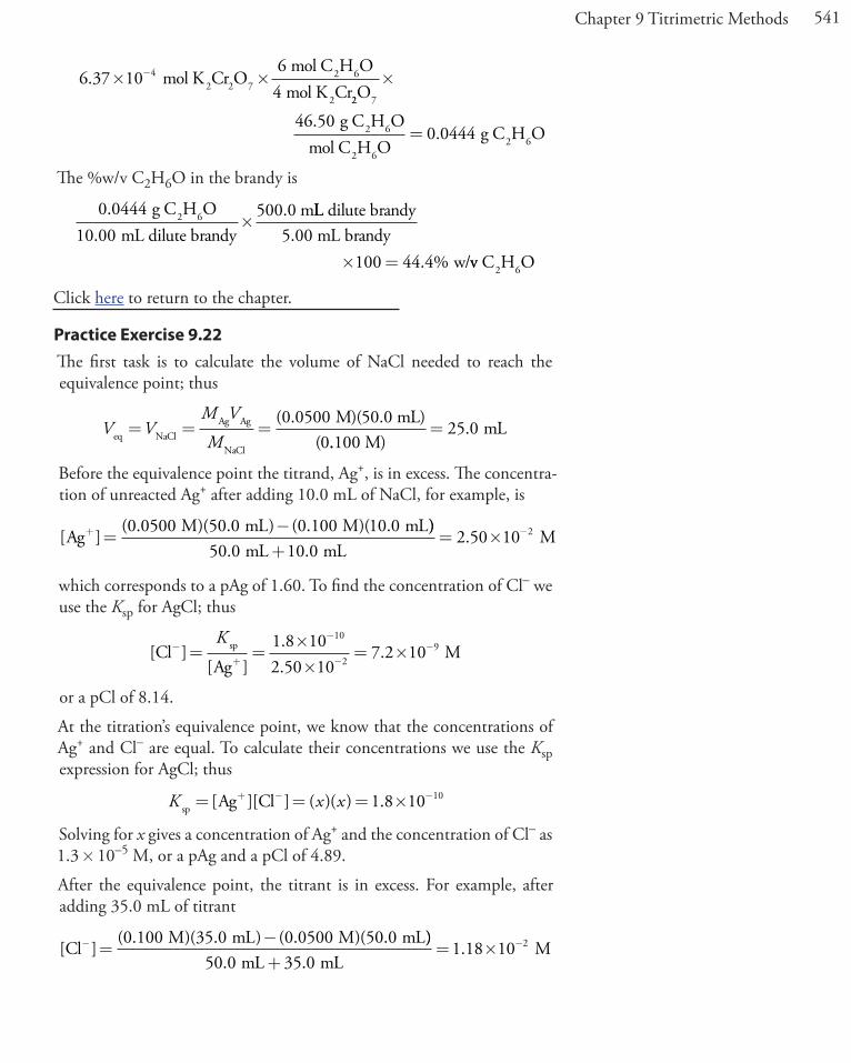
541Chapter 9 Titrimetric Methods
6 37 10 4. � �− mol K Cr O6 mol C H O
4 mol K Cr2 2 72 6
2 22 7
2 6
2 62 6
O
g C H Omol C H O
g C H O
�
=46 50
0 0444.
.
The %w/v C2H6O in the brandy is
0 044410 00
500 0..
.g C H OmL dilute brandy
m2 6 �LL dilute brandy
5.00 mL brandyw/� =100 44 4. % vv C H O2 6
Click here to return to the chapter.
Practice Exercise 9.22The first task is to calculate the volume of NaCl needed to reach the equivalence point; thus
V VM V
Meq NaClAg Ag
NaCl
M)(50.0 mL)(0
= = =( .0 0500
..100 M)mL= 25 0.
Before the equivalence point the titrand, Ag+, is in excess. The concentra-tion of unreacted Ag+ after adding 10.0 mL of NaCl, for example, is
[ ]( . )( . ) ( . )( .
AgM mL M mL+ =
−0 0500 50 0 0 100 10 0 )). .
.50 0 10 0
2 50 10 2
mL mLM
+= � −
which corresponds to a pAg of 1.60. To find the concentration of Cl– we use the Ksp for AgCl; thus
[ ][ ]
..
.ClAg
Msp−+
−
−−= =
��
= �K 1 8 10
2 50 107 2 10
10
29
or a pCl of 8.14.
At the titration’s equivalence point, we know that the concentrations of Ag+ and Cl– are equal. To calculate their concentrations we use the Ksp expression for AgCl; thus
K x xsp Ag Cl= = = �+ − −[ ][ ] ( )( ) .1 8 10 10
Solving for x gives a concentration of Ag+ and the concentration of Cl– as 1.3 � 10–5 M, or a pAg and a pCl of 4.89.
After the equivalence point, the titrant is in excess. For example, after adding 35.0 mL of titrant
[ ]( . )( . ) ( . )( .
ClM mL M mL− =
−0 100 35 0 0 0500 50 0 )). .
.50 0 35 0
1 18 10 2
mL mLM
+= � −

542 Analytical Chemistry 2.0
or a pCl of 1.93. To find the concentration of Ag+ we use the Ksp for AgCl; thus
[ ][ ]
..
.AgCl
Msp+−
−
−−= =
��
= �K 1 8 10
1 18 101 5 10
10
28
or a pAg of 7.82. The following table summarizes additional results for this titration.
Volume of NaCl (mL) pAg pCl
0 1.30 –5.00 1.44 8.31
10.0 1.60 8.1415.0 1.81 7.9320.0 2.15 7.6025.0 4.89 4.8930.0 7.54 2.2035.0 7.82 1.9340.0 7.97 1.7845.0 8.07 1.6850.0 8.14 1.60
Click here to return to the chapter.
Practice Exercise 9.23The titration uses
0 10780 02719 2 931 10 3.. .
M KSCNL
L mol KSC� = � − NN
The stoichiometry between SCN– and Ag+ is 1:1; thus, there are
2 931 10107 87
0 31623..
.� � =− +mol Agg Ag
mol Agg Ag
in the 25.00 mL sample. Because this represents ¼ of the total solution, there are 0.3162 � 4 or 1.265 g Ag in the alloy. The %w/w Ag in the al-loy is
1 265100 64 44
.. %
g Ag1.963 g sample
w/w Ag� =
Click here to return to the chapter.
Related Documents