Chapter 7 Load Balancing and Termination Detectionftp.gunadarma.ac.id/handouts/S1-Sistem Komputer/Pengolahan Paralel...Page 153 Slides for Parallel Programming: Techniques and Applications

Page 152

Slides for Parallel Programming: Techniques and Applications using Networked Workstations and Parallel ComputersBarry Wilkinson and Michael Allen Prentice Hall, 1999. All rights reserved.

Chapter 7Load Balancing and Termination

Detection

Load balancing – used to distribute computations fairly across processors in order to

obtain the highest possible execution speed.

Termination detection – detecting when a computation has been completed. More

difficult when the computaion is distributed.

P4

P5

P0

P1

P2

P3

P4

P5

P2P1P0

P3

Time

(b) Perfect load balancing

(a) Imperfect load balancing leading

t

Figure 7.1 Load balancing.

to increased execution time

Processors

Processors

Page 153


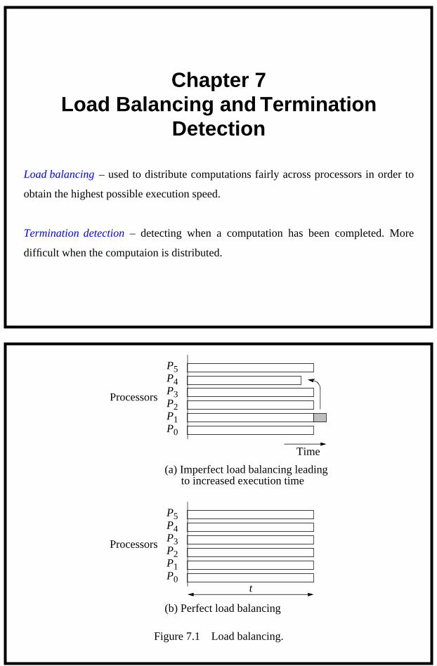
Static Load Balancing

Before the execution of any process. Some potential static load-balancing techniques:

• Round robin algorithm — passes out tasks in sequential order of processes coming

back to the first when all processes have been given a task

• Randomized algorithms — selects processes at random to take tasks

• Recursive bisection — recursively divides the problem into subproblems of equal

computational effort while minimizing message passing

• Simulated annealing — an optimization technique

• Genetic algorithm — another optimization technique, described in Chapter 12

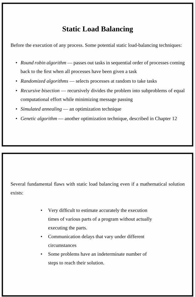
Several fundamental flaws with static load balancing even if a mathematical solution

exists:

• Very difficult to estimate accurately the execution

times of various parts of a program without actually

executing the parts.

• Communication delays that vary under different

circumstances

• Some problems have an indeterminate number of

steps to reach their solution.

Page 154


Dynamic Load Balancing

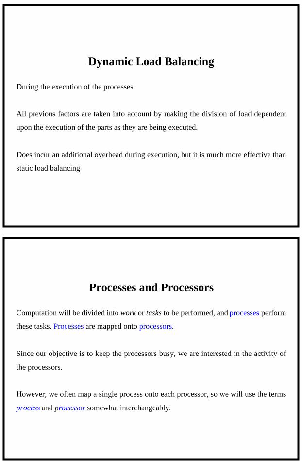
During the execution of the processes.

All previous factors are taken into account by making the division of load dependent

upon the execution of the parts as they are being executed.

Does incur an additional overhead during execution, but it is much more effective than

static load balancing

Processes and Processors

Computation will be divided into work or tasks to be performed, and processes perform

these tasks. Processes are mapped onto processors.

Since our objective is to keep the processors busy, we are interested in the activity of

the processors.

However, we often map a single process onto each processor, so we will use the terms

process and processor somewhat interchangeably.

Page 155


Dynamic Load Balancing

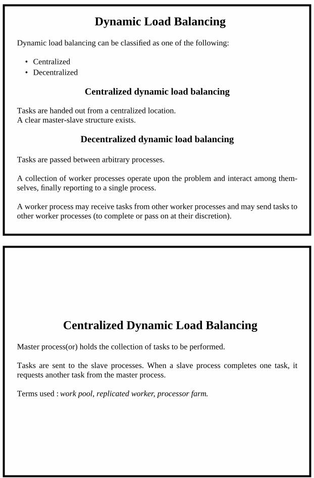
Dynamic load balancing can be classified as one of the following:

• Centralized • Decentralized

Centralized dynamic load balancing

Tasks are handed out from a centralized location. A clear master-slave structure exists.

Decentralized dynamic load balancing

Tasks are passed between arbitrary processes.

A collection of worker processes operate upon the problem and interact among them-selves, finally reporting to a single process.

A worker process may receive tasks from other worker processes and may send tasks toother worker processes (to complete or pass on at their discretion).

Centralized Dynamic Load Balancing

Master process(or) holds the collection of tasks to be performed.

Tasks are sent to the slave processes. When a slave process completes one task, itrequests another task from the master process.

Terms used : work pool, replicated worker, processor farm.

Page 156


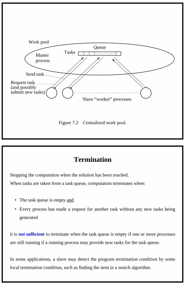
QueueWork pool

Slave “worker” processes

Masterprocess

Figure 7.2 Centralized work pool.

Tasks

Request task

Send task

(and possiblysubmit new tasks)

Termination

Stopping the computation when the solution has been reached.

When tasks are taken from a task queue, computation terminates when:

• The task queue is empty and

• Every process has made a request for another task without any new tasks being

generated

it is not sufficient to terminate when the task queue is empty if one or more processes

are still running if a running process may provide new tasks for the task queue.

In some applications, a slave may detect the program termination condition by some

local termination condition, such as finding the item in a search algorithm.

Page 157


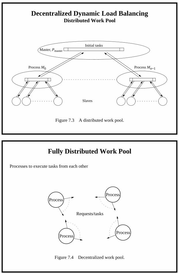
Process M0 Process Mn−1

Master, Pmaster

Slaves

Initial tasks

Figure 7.3 A distributed work pool.

Decentralized Dynamic Load BalancingDistributed Work Pool

Process

Requests/tasks

ProcessProcess

Process

Figure 7.4 Decentralized work pool.

Fully Distributed Work Pool

Processes to execute tasks from each other

Page 158


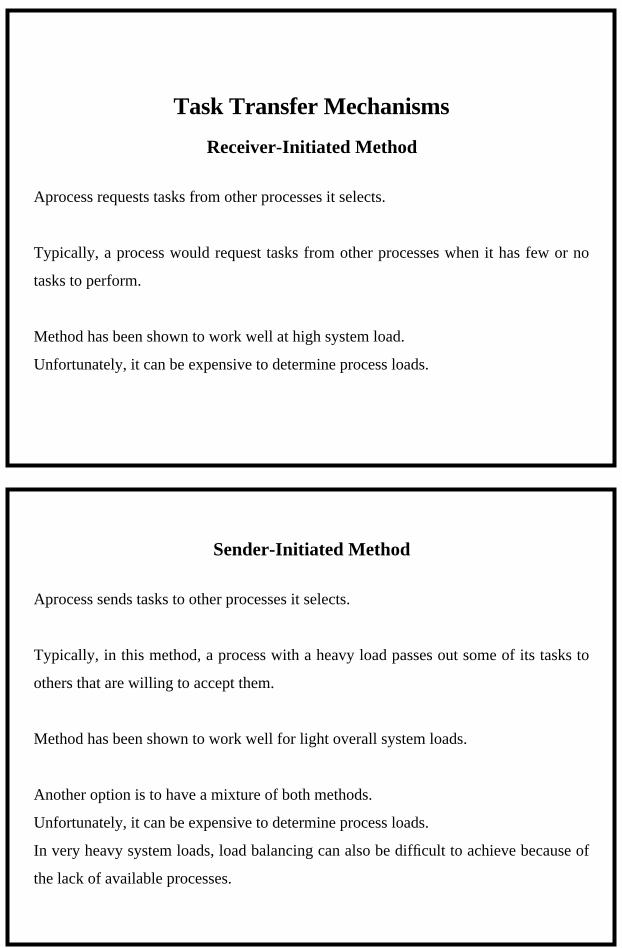
Task Transfer Mechanisms

Receiver-Initiated Method

Aprocess requests tasks from other processes it selects.

Typically, a process would request tasks from other processes when it has few or no

tasks to perform.

Method has been shown to work well at high system load.

Unfortunately, it can be expensive to determine process loads.

Sender-Initiated Method

Aprocess sends tasks to other processes it selects.

Typically, in this method, a process with a heavy load passes out some of its tasks to

others that are willing to accept them.

Method has been shown to work well for light overall system loads.

Another option is to have a mixture of both methods.

Unfortunately, it can be expensive to determine process loads.

In very heavy system loads, load balancing can also be difficult to achieve because of

the lack of available processes.

Page 159


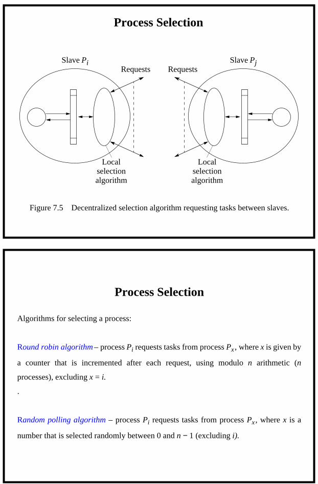
Figure 7.5 Decentralized selection algorithm requesting tasks between slaves.

RequestsSlave Pi

Localselectionalgorithm

RequestsSlave Pj

Localselectionalgorithm

Process Selection

Process Selection

Algorithms for selecting a process:

Round robin algorithm – process Pi requests tasks from process Px , where x is given by

a counter that is incremented after each request, using modulo n arithmetic (n

processes), excluding x = i.

.

Random polling algorithm – process Pi requests tasks from process Px , where x is a

number that is selected randomly between 0 and n − 1 (excluding i).

Page 160


Masterprocess

P1 P2 P3 Pn−1

P0

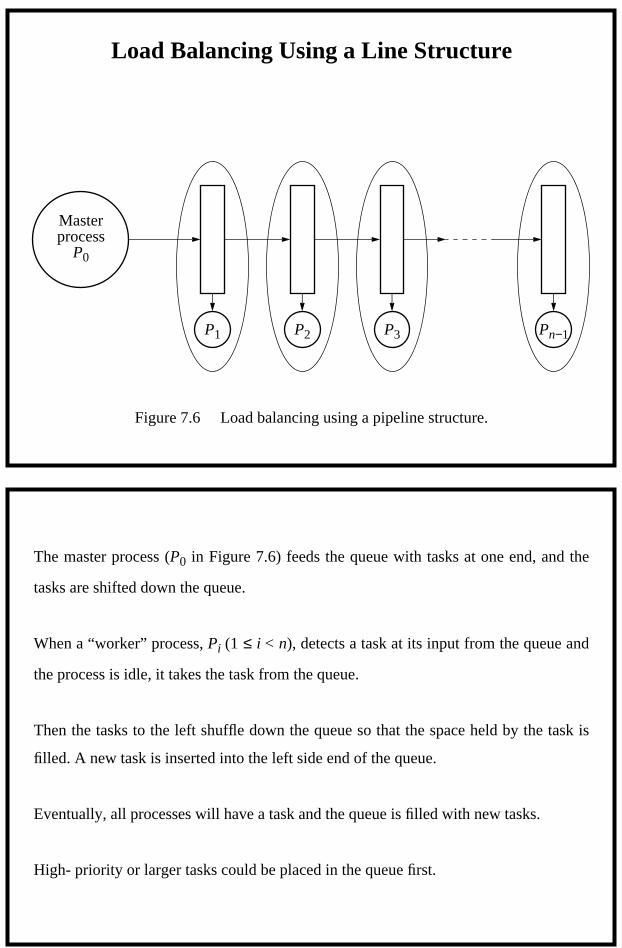
Figure 7.6 Load balancing using a pipeline structure.

Load Balancing Using a Line Structure

The master process (P0 in Figure 7.6) feeds the queue with tasks at one end, and the

tasks are shifted down the queue.

When a “worker” process, Pi (1 ≤ i < n), detects a task at its input from the queue and

the process is idle, it takes the task from the queue.

Then the tasks to the left shuffle down the queue so that the space held by the task is

filled. A new task is inserted into the left side end of the queue.

Eventually, all processes will have a task and the queue is filled with new tasks.

High- priority or larger tasks could be placed in the queue first.

Page 161


If buffer empty,make request

Receive taskfrom request

If free,requesttask

Receivetask fromrequest

If buffer full,send task

Request for task

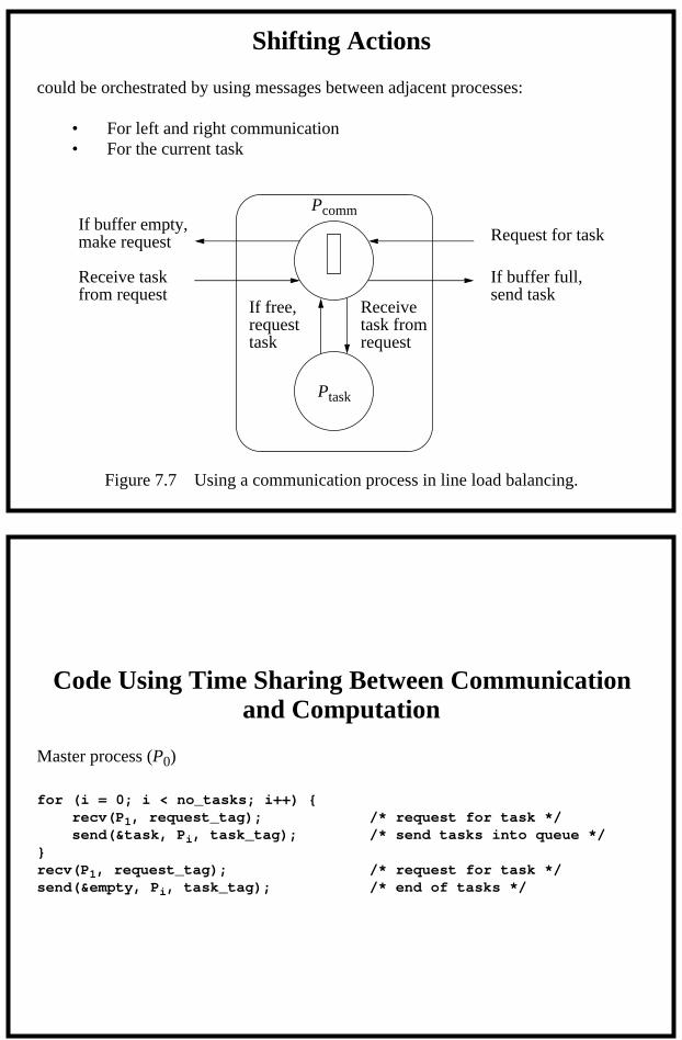
Figure 7.7 Using a communication process in line load balancing.

Ptask

Pcomm

Shifting Actions

could be orchestrated by using messages between adjacent processes:

• For left and right communication• For the current task

Code Using Time Sharing Between Communication and Computation

Master process (P0)

for (i = 0; i < no_tasks; i++) {recv(P1, request_tag); /* request for task */send(&task, Pi, task_tag); /* send tasks into queue */

}recv(P1, request_tag); /* request for task */send(&empty, Pi, task_tag); /* end of tasks */

Page 162


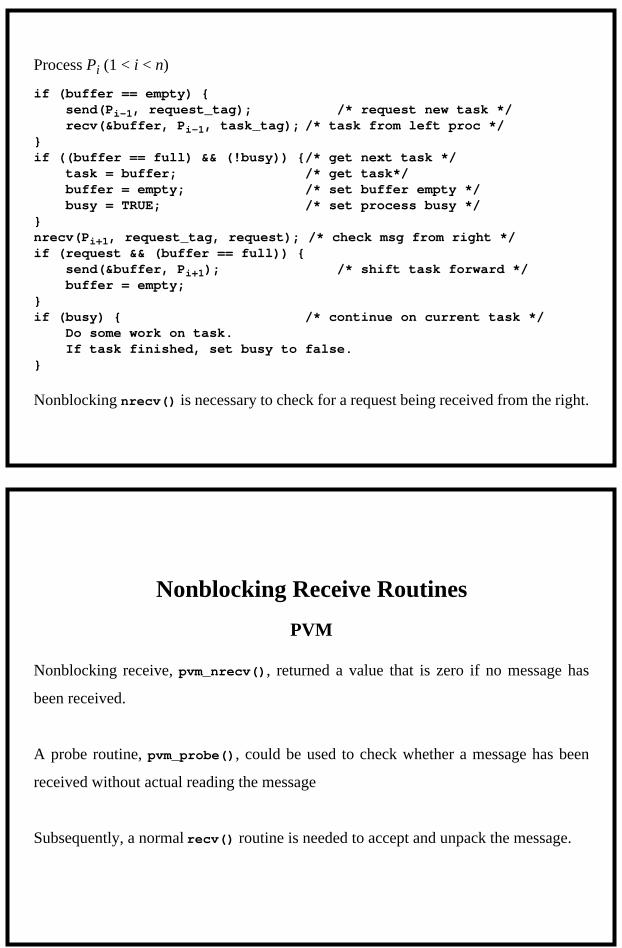
Process Pi (1 < i < n)

if (buffer == empty) {send(Pi-1, request_tag); /* request new task */recv(&buffer, Pi-1, task_tag); /* task from left proc */

}if ((buffer == full) && (!busy)) {/* get next task */

task = buffer; /* get task*/buffer = empty; /* set buffer empty */busy = TRUE; /* set process busy */

}nrecv(Pi+1, request_tag, request); /* check msg from right */if (request && (buffer == full)) {

send(&buffer, Pi+1); /* shift task forward */buffer = empty;

}if (busy) { /* continue on current task */

Do some work on task.If task finished, set busy to false.

}

Nonblocking nrecv() is necessary to check for a request being received from the right.

Nonblocking Receive Routines

PVM

Nonblocking receive, pvm_nrecv(), returned a value that is zero if no message has

been received.

A probe routine, pvm_probe(), could be used to check whether a message has been

received without actual reading the message

Subsequently, a normal recv() routine is needed to accept and unpack the message.

Page 163


Nonblocking Receive Routines

MPI

Nonblocking receive, MPI_Irecv(), returns a request “handle,” which is used in

subsequent completion routines to wait for the message or to establish whether the

message has actually been received at that point (MPI_Wait() and MPI_Test(),

respectively).

In effect, the nonblocking receive, MPI_Irecv(), posts a request for message and

returns immediately.

P0

P1

P3

P2

P6P4P5

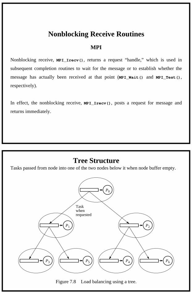
Figure 7.8 Load balancing using a tree.

Taskwhenrequested

Tree StructureTasks passed from node into one of the two nodes below it when node buffer empty.

Page 164


Distributed Termination Detection Algorithms

Termination Conditions

At time t requires the following conditions to be satisfied:

• Application-specific local termination conditions exist throughout the collection of

processes, at time t.

• There are no messages in transit between processes at time t.

Subtle difference between these termination conditions and those given for a centralized

load-balancing system is having to take into account messages in transit.

Second condition is necessary for the distributed termination system because a message

in transit might restart a terminated process. More difficult to recognize. The time that it

takes for messages to travel between processes will not be known in advance.

Using Acknowledgment Messages

Each process in one of two states:

1. Inactive - without any task to perform2. Active

The process that sent the task to make it enter the active state becomes its “parent.”

On every occasion when process receives a task, it immediately sends an acknowledg-ment message, except if the process it receives the task from is its parent process.

It only sends an acknowledgment message to its parent when it is ready to becomeinactive, i.e. when

• Its local termination condition exists (all tasks are completed).• It has transmitted all its acknowledgments for tasks it has received.• It has received all its acknowledgments for tasks it has sent out.

The last condition means that a process must become inactive before its parent process.When the first process becomes idle, the computation can terminate.

Page 165


Inactive

Active

Parent

First task

Other processes

Finalacknowledgment

Process

TaskAcknowledgment

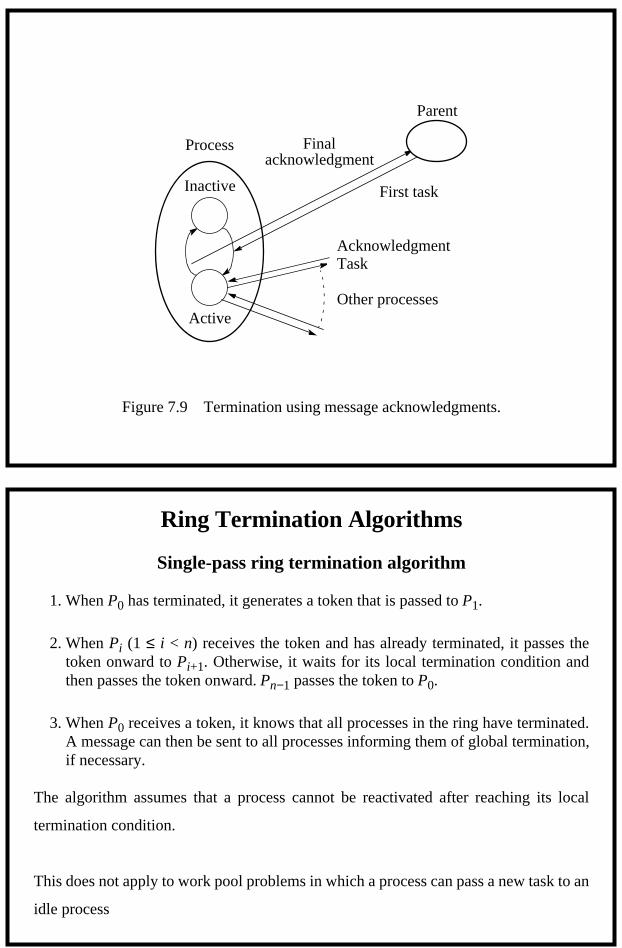
Figure 7.9 Termination using message acknowledgments.

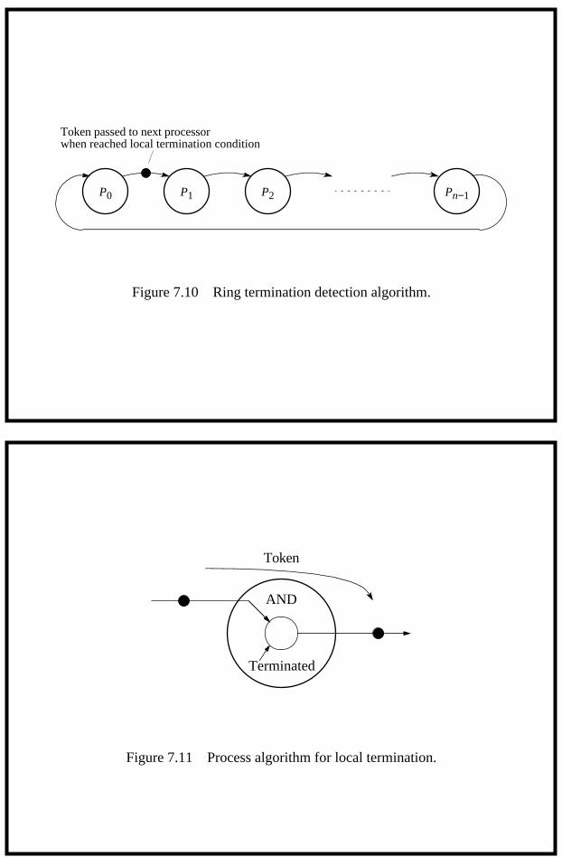
Ring Termination Algorithms

Single-pass ring termination algorithm

1. When P0 has terminated, it generates a token that is passed to P1.

2. When Pi (1 ≤ i < n) receives the token and has already terminated, it passes thetoken onward to Pi+1. Otherwise, it waits for its local termination condition andthen passes the token onward. Pn−1 passes the token to P0.

3. When P0 receives a token, it knows that all processes in the ring have terminated.A message can then be sent to all processes informing them of global termination,if necessary.

The algorithm assumes that a process cannot be reactivated after reaching its local

termination condition.

This does not apply to work pool problems in which a process can pass a new task to an

idle process

Page 166


P0 P2P1 Pn−1

Token passed to next processor

Figure 7.10 Ring termination detection algorithm.

when reached local termination condition

Terminated

Token

AND

Figure 7.11 Process algorithm for local termination.

Page 167


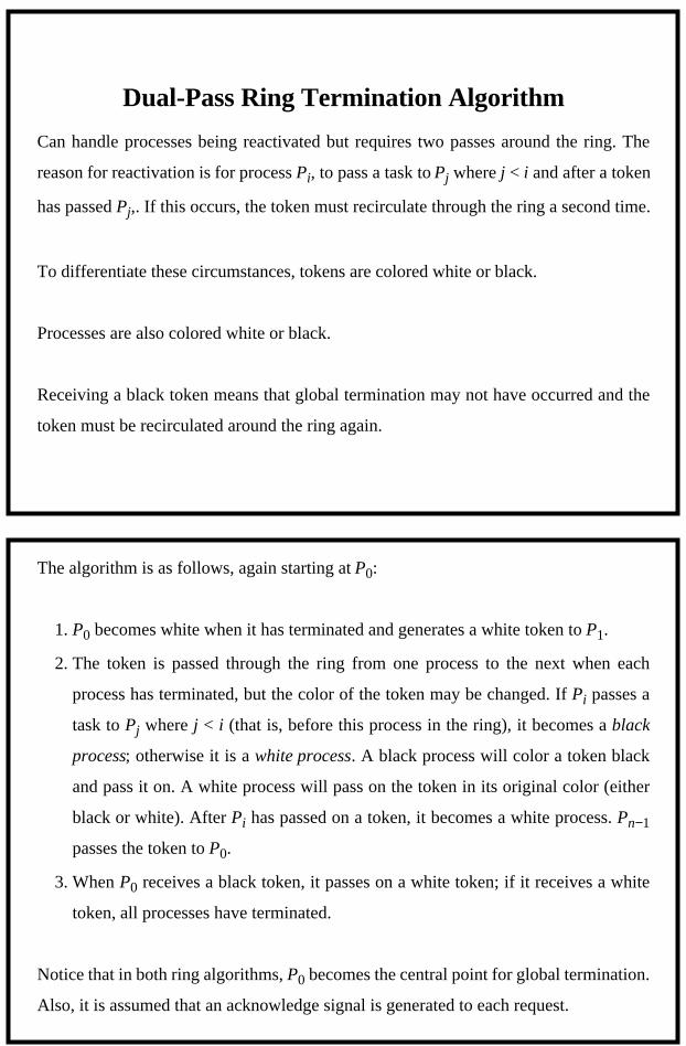
Dual-Pass Ring Termination Algorithm

Can handle processes being reactivated but requires two passes around the ring. The

reason for reactivation is for process Pi, to pass a task to Pj where j < i and after a token

has passed Pj,. If this occurs, the token must recirculate through the ring a second time.

To differentiate these circumstances, tokens are colored white or black.

Processes are also colored white or black.

Receiving a black token means that global termination may not have occurred and the

token must be recirculated around the ring again.

The algorithm is as follows, again starting at P0:

1. P0 becomes white when it has terminated and generates a white token to P1.

2. The token is passed through the ring from one process to the next when each

process has terminated, but the color of the token may be changed. If Pi passes a

task to Pj where j < i (that is, before this process in the ring), it becomes a black

process; otherwise it is a white process. A black process will color a token black

and pass it on. A white process will pass on the token in its original color (either

black or white). After Pi has passed on a token, it becomes a white process. Pn−1

passes the token to P0.

3. When P0 receives a black token, it passes on a white token; if it receives a white

token, all processes have terminated.

Notice that in both ring algorithms, P0 becomes the central point for global termination.

Also, it is assumed that an acknowledge signal is generated to each request.

Page 168


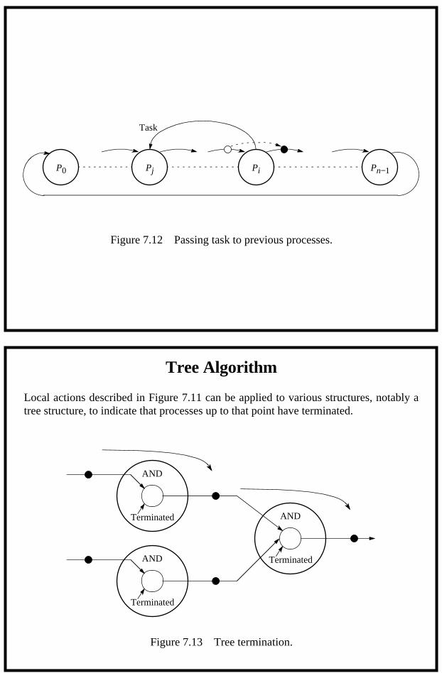
P0 PiPj Pn−1

Figure 7.12 Passing task to previous processes.

Task

Terminated

AND

Terminated

AND Terminated

AND

Figure 7.13 Tree termination.

Tree Algorithm

Local actions described in Figure 7.11 can be applied to various structures, notably atree structure, to indicate that processes up to that point have terminated.

Page 169


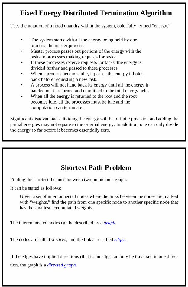
Fixed Energy Distributed Termination Algorithm

Uses the notation of a fixed quantity within the system, colorfully termed “energy.”

• The system starts with all the energy being held by one process, the master process.

• Master process passes out portions of the energy with the tasks to processes making requests for tasks.

• If these processes receive requests for tasks, the energy is divided further and passed to these processes.

• When a process becomes idle, it passes the energy it holds back before requesting a new task.

• A process will not hand back its energy until all the energy it handed out is returned and combined to the total energy held.

• When all the energy is returned to the root and the root becomes idle, all the processes must be idle and the computation can terminate.

Significant disadvantage - dividing the energy will be of finite precision and adding thepartial energies may not equate to the original energy. In addition, one can only dividethe energy so far before it becomes essentially zero.

Shortest Path Problem

Finding the shortest distance between two points on a graph.

It can be stated as follows:

Given a set of interconnected nodes where the links between the nodes are markedwith “weights,” find the path from one specific node to another specific node thathas the smallest accumulated weights.

The interconnected nodes can be described by a graph.

The nodes are called vertices, and the links are called edges.

If the edges have implied directions (that is, an edge can only be traversed in one direc-

tion, the graph is a directed graph.

Page 170


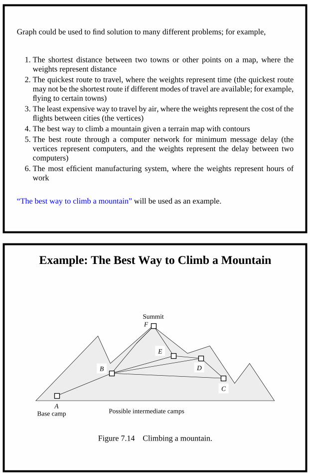
Graph could be used to find solution to many different problems; for example,

1. The shortest distance between two towns or other points on a map, where theweights represent distance

2. The quickest route to travel, where the weights represent time (the quickest routemay not be the shortest route if different modes of travel are available; for example,flying to certain towns)

3. The least expensive way to travel by air, where the weights represent the cost of theflights between cities (the vertices)

4. The best way to climb a mountain given a terrain map with contours5. The best route through a computer network for minimum message delay (the

vertices represent computers, and the weights represent the delay between twocomputers)

6. The most efficient manufacturing system, where the weights represent hours ofwork

“The best way to climb a mountain” will be used as an example.

Base camp

Summit

Possible intermediate camps

B

C

A

Figure 7.14 Climbing a mountain.

F

E

D

Example: The Best Way to Climb a Mountain

Page 171


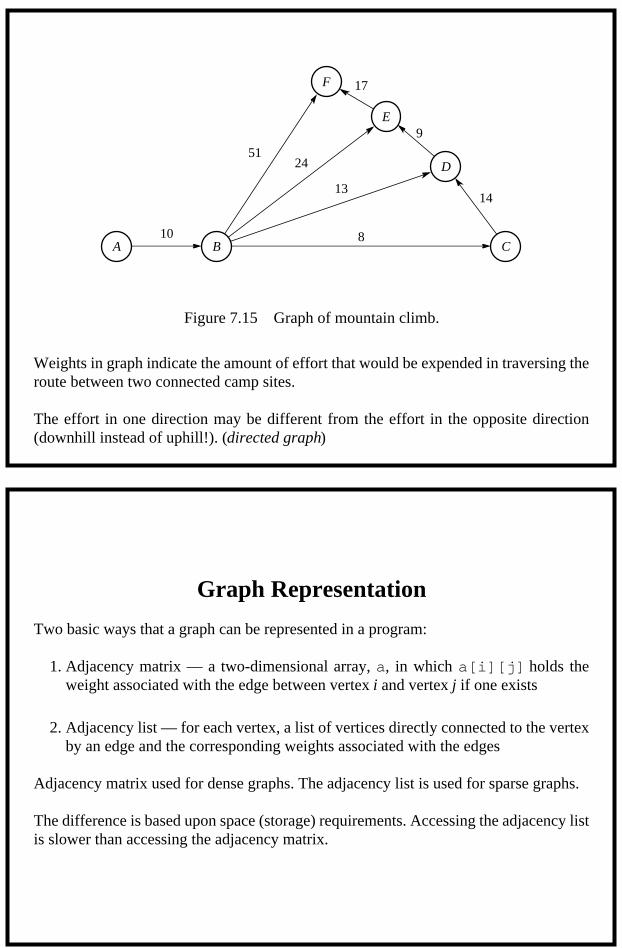
Figure 7.15 Graph of mountain climb.

A B C

D

E

F

10

13

17

51

8

24

9

14

Weights in graph indicate the amount of effort that would be expended in traversing theroute between two connected camp sites.

The effort in one direction may be different from the effort in the opposite direction(downhill instead of uphill!). (directed graph)

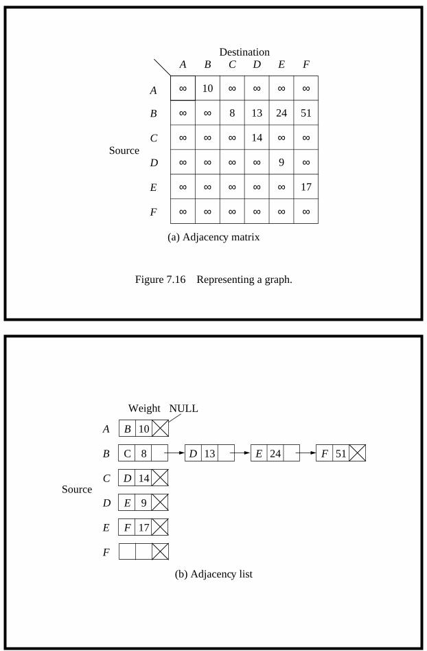
Graph Representation

Two basic ways that a graph can be represented in a program:

1. Adjacency matrix — a two-dimensional array, a, in which a[i][j] holds theweight associated with the edge between vertex i and vertex j if one exists

2. Adjacency list — for each vertex, a list of vertices directly connected to the vertexby an edge and the corresponding weights associated with the edges

Adjacency matrix used for dense graphs. The adjacency list is used for sparse graphs.

The difference is based upon space (storage) requirements. Accessing the adjacency listis slower than accessing the adjacency matrix.

Page 172


A

B

C

D

E

F

A B C D E F

∞

∞

∞

∞

∞

∞

10

13

17

518 24

9

∞

∞

∞ ∞ ∞ ∞ ∞

∞

∞ ∞

∞∞

∞

∞

∞

∞

∞ ∞ ∞ ∞

∞

∞14Source

Destination

(a) Adjacency matrix

Figure 7.16 Representing a graph.

A

B

C

D

E

F

Source

Weight NULL

10

8 13 24 51C D E F

14D

9E

17F

(b) Adjacency list

B

Page 173


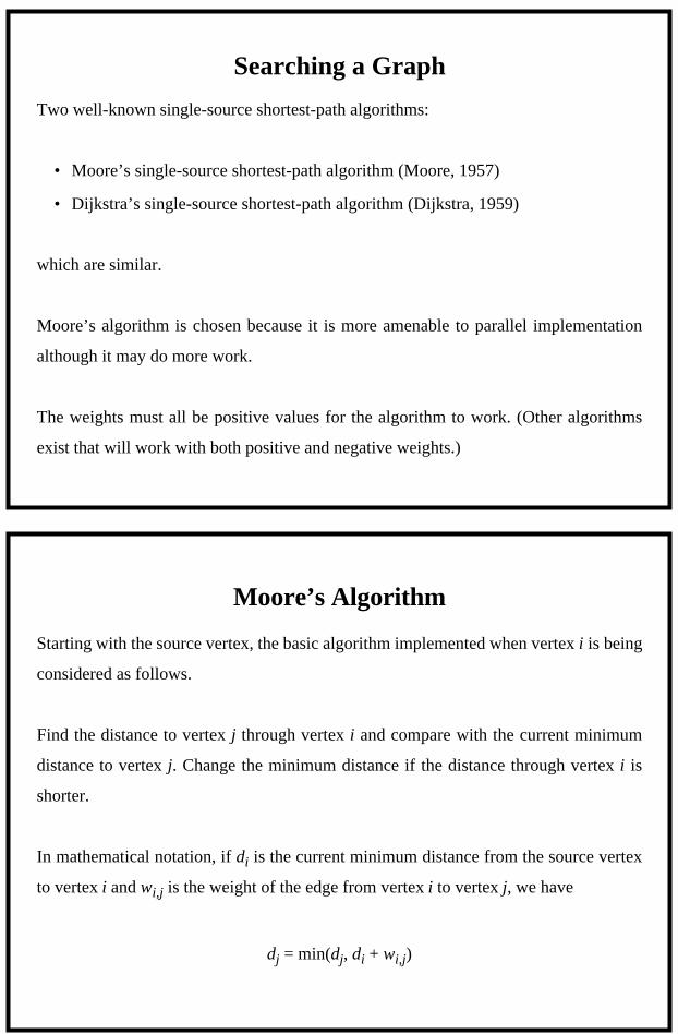
Searching a Graph

Two well-known single-source shortest-path algorithms:

• Moore’s single-source shortest-path algorithm (Moore, 1957)

• Dijkstra’s single-source shortest-path algorithm (Dijkstra, 1959)

which are similar.

Moore’s algorithm is chosen because it is more amenable to parallel implementation

although it may do more work.

The weights must all be positive values for the algorithm to work. (Other algorithms

exist that will work with both positive and negative weights.)

Moore’s Algorithm

Starting with the source vertex, the basic algorithm implemented when vertex i is being

considered as follows.

Find the distance to vertex j through vertex i and compare with the current minimum

distance to vertex j. Change the minimum distance if the distance through vertex i is

shorter.

In mathematical notation, if di is the current minimum distance from the source vertex

to vertex i and wi,j is the weight of the edge from vertex i to vertex j, we have

dj = min(dj, di + wi,j)

Page 174


Vertex i

Vertex j

wi,j

dj

di

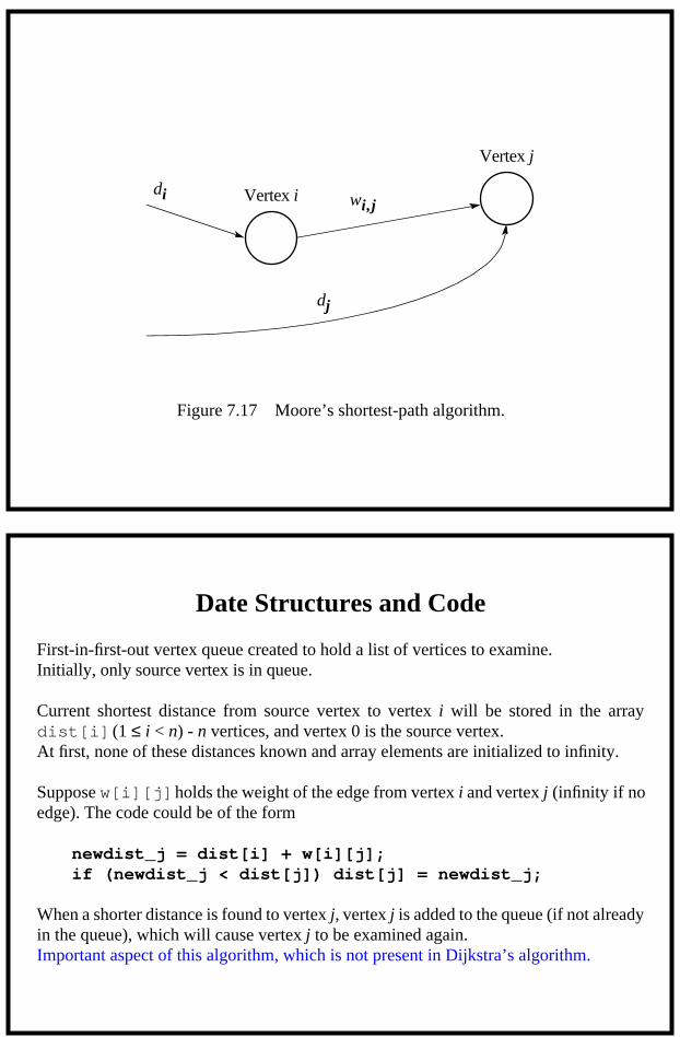
Figure 7.17 Moore’s shortest-path algorithm.

Date Structures and Code

First-in-first-out vertex queue created to hold a list of vertices to examine.Initially, only source vertex is in queue.

Current shortest distance from source vertex to vertex i will be stored in the arraydist[i] (1 ≤ i < n) - n vertices, and vertex 0 is the source vertex.At first, none of these distances known and array elements are initialized to infinity.

Suppose w[i][j] holds the weight of the edge from vertex i and vertex j (infinity if noedge). The code could be of the form

newdist_j = dist[i] + w[i][j];if (newdist_j < dist[j]) dist[j] = newdist_j;

When a shorter distance is found to vertex j, vertex j is added to the queue (if not alreadyin the queue), which will cause vertex j to be examined again.Important aspect of this algorithm, which is not present in Dijkstra’s algorithm.

Page 175


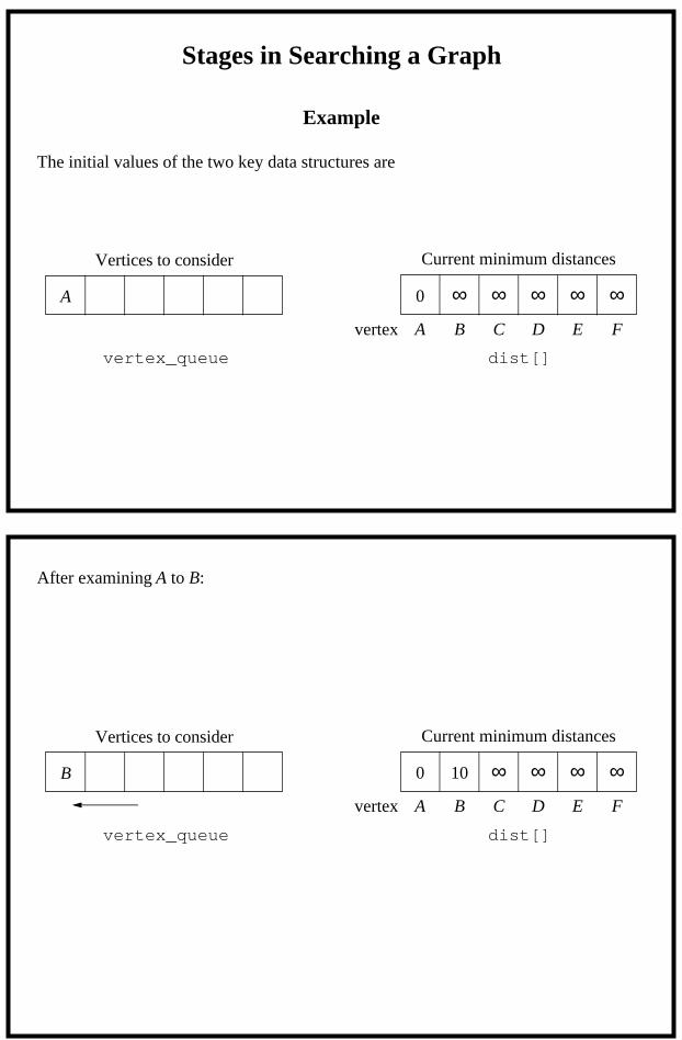
Stages in Searching a Graph

Example

The initial values of the two key data structures are

Vertices to consider

vertex

Current minimum distances

dist[]vertex_queue

A 0 ∞∞ ∞∞∞A B C D E F

After examining A to B:


vertex


dist[]vertex_queue

B 0 ∞10 ∞∞∞A B C D E F

Page 176


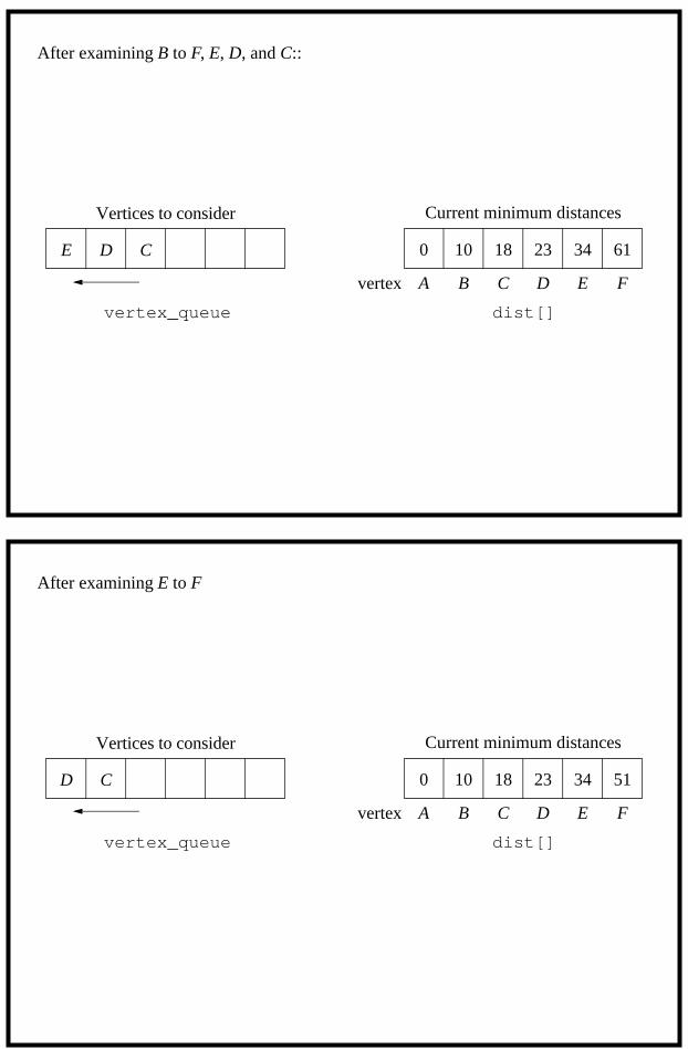
After examining B to F, E, D, and C::


vertex


dist[]vertex_queue

E D 0 6110C 342318

A B C D E F

After examining E to F


vertex


dist[]vertex_queue

D C 0 5110 342318

A B C D E F

Page 177


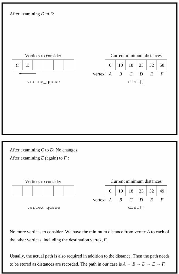
After examining D to E:


vertex


dist[]vertex_queue

C E 0 5010 322318

A B C D E F

After examining C to D: No changes.

After examining E (again) to F :


vertex


dist[]vertex_queue

0 4910 322318

A B C D E F

No more vertices to consider. We have the minimum distance from vertex A to each of

the other vertices, including the destination vertex, F.

Usually, the actual path is also required in addition to the distance. Then the path needs

to be stored as distances are recorded. The path in our case is A → B → D → E → F.

Page 178


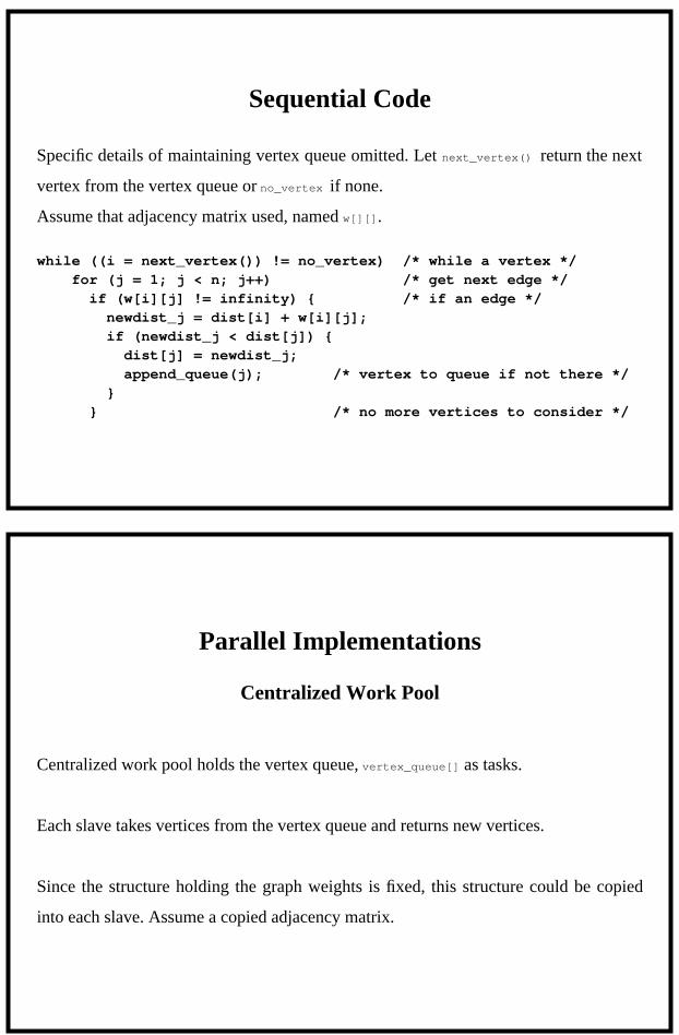
Sequential Code

Specific details of maintaining vertex queue omitted. Let next_vertex() return the next

vertex from the vertex queue or no_vertex if none.

Assume that adjacency matrix used, named w[][].

while ((i = next_vertex()) != no_vertex) /* while a vertex */for (j = 1; j < n; j++) /* get next edge */if (w[i][j] != infinity) { /* if an edge */newdist_j = dist[i] + w[i][j];if (newdist_j < dist[j]) {dist[j] = newdist_j;append_queue(j); /* vertex to queue if not there */

}} /* no more vertices to consider */

Parallel Implementations

Centralized Work Pool

Centralized work pool holds the vertex queue, vertex_queue[] as tasks.

Each slave takes vertices from the vertex queue and returns new vertices.

Since the structure holding the graph weights is fixed, this structure could be copied

into each slave. Assume a copied adjacency matrix.

Page 179


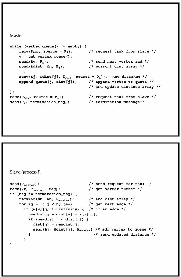
Master

while (vertex_queue() != empty) {recv(PANY, source = Pi); /* request task from slave */v = get_vertex_queue();send(&v, Pi); /* send next vertex and */send(&dist, &n, Pi); /* current dist array */.

recv(&j, &dist[j], PANY, source = Pi);/* new distance */append_queue(j, dist[j]); /* append vertex to queue */

/* and update distance array */};recv(PANY, source = Pi); /* request task from slave */send(Pi, termination_tag); /* termination message*/

Slave (process i)

send(Pmaster); /* send request for task */recv(&v, Pmaster, tag); /* get vertex number */if (tag != termination_tag) {

recv(&dist, &n, Pmaster); /* and dist array */for (j = 1; j < n; j++) /* get next edge */if (w[v][j] != infinity) { /* if an edge */newdist_j = dist[v] + w[v][j];if (newdist_j < dist[j]) {dist[j] = newdist_j;send(&j, &dist[j], Pmaster);/* add vertex to queue */

} /* send updated distance */}

}

Page 180


Decentralized Work Pool

Convenient approach is to assign slave process i to search around vertex i only and for

it to have the vertex queue entry for vertex i if this exists in the queue.

The array dist[] will also be distributed among the processes so that process i

maintains the current minimum distance to vertex i.

Process i also stores an adjacency matrix/list for vertex i, for the purpose of identifying

the edges from vertex i.

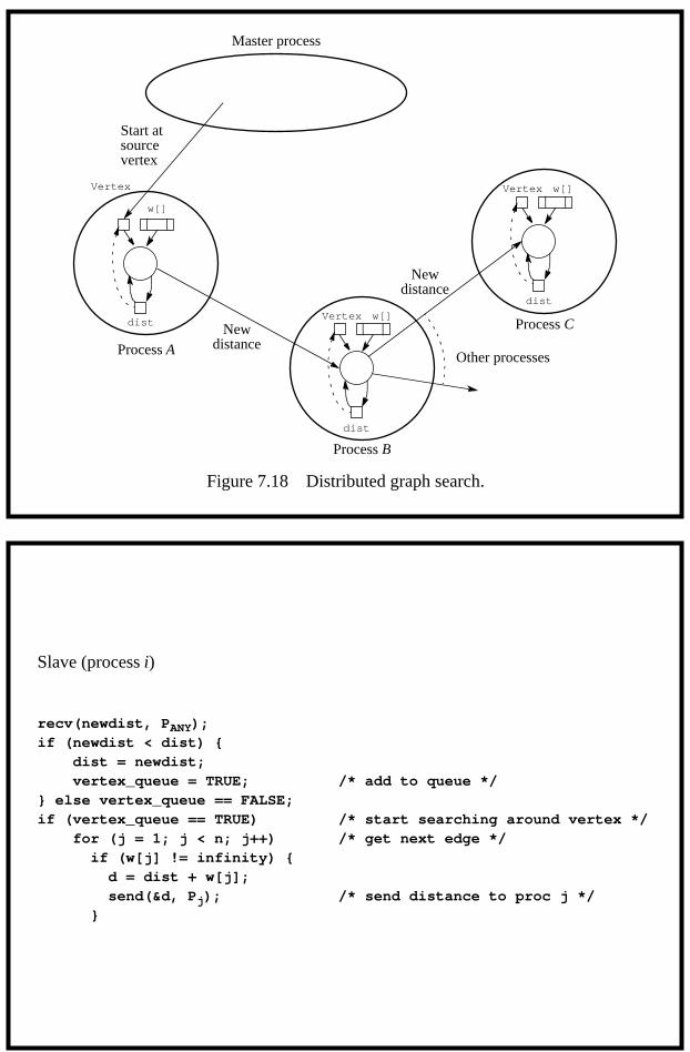
Search Algorithm

Search activated by loading source vertex into the appropriate process.

Vertex A is the first vertex to search. The process assigned to vertex A is activated.

This process will search around its vertex to find distances to connected vertices.

Distance to process j will be sent to process j for it to compare with its currently stored

value and replace if the currently stored value is larger.

In this fashion, all minimum distances will be updated during the search.

If the contents of d[i] changes, process i will be reactivated to search again.

Page 181


Start at

w[]

dist Process C

Process A

Master process

Figure 7.18 Distributed graph search.

Vertex

sourcevertex

w[]

dist

Vertex

dist

Process B

Newdistance

Newdistance

w[]Vertex

Other processes

Slave (process i)

recv(newdist, PANY);if (newdist < dist) {

dist = newdist;vertex_queue = TRUE; /* add to queue */

} else vertex_queue == FALSE;if (vertex_queue == TRUE) /* start searching around vertex */

for (j = 1; j < n; j++) /* get next edge */if (w[j] != infinity) {d = dist + w[j];send(&d, Pj); /* send distance to proc j */

}

Page 182


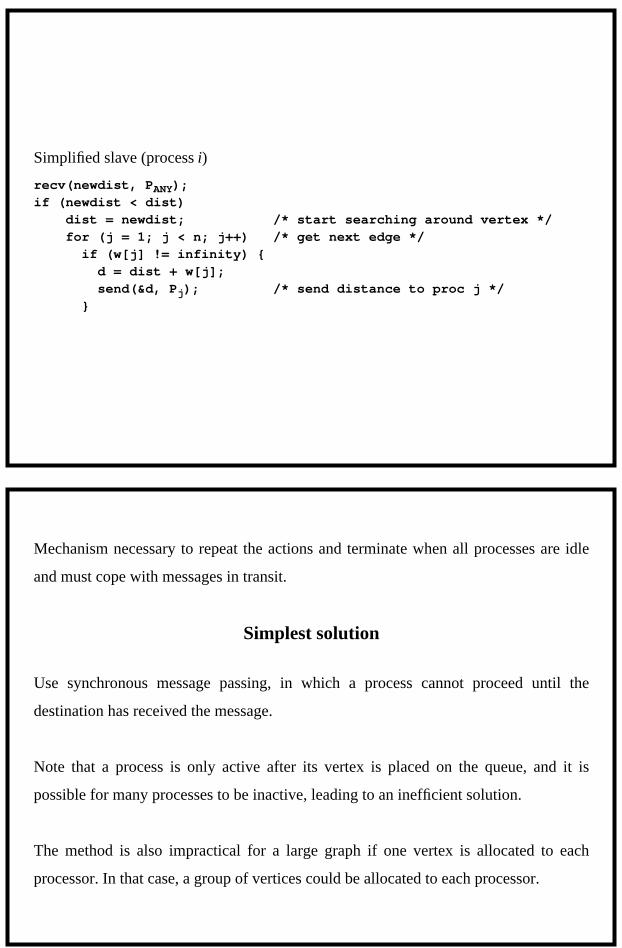
Simplified slave (process i)

recv(newdist, PANY);if (newdist < dist)

dist = newdist; /* start searching around vertex */for (j = 1; j < n; j++) /* get next edge */if (w[j] != infinity) {d = dist + w[j];send(&d, Pj); /* send distance to proc j */

}

Mechanism necessary to repeat the actions and terminate when all processes are idle

and must cope with messages in transit.

Simplest solution

Use synchronous message passing, in which a process cannot proceed until the

destination has received the message.

Note that a process is only active after its vertex is placed on the queue, and it is

possible for many processes to be inactive, leading to an inefficient solution.

The method is also impractical for a large graph if one vertex is allocated to each

processor. In that case, a group of vertices could be allocated to each processor.

Chapter 7 Load Balancing and Termination Detectionftp.gunadarma.ac.id/handouts/S1-Sistem Komputer/Pengolahan Paralel...Page 153 Slides for Parallel Programming: Techniques and Applications

Documents