Chapter 5 office2007 black and white

12/10/2007

1

The Multiple Regression Model

Prepared by Vera Tabakova, East Carolina University

5.1 Model Specification and Data5.2 Estimating the Parameters of the Multiple

Regression Model5 3 S li P ti f th L t S5.3 Sampling Properties of the Least Squares

Estimator5.4 Interval Estimation5.5 Hypothesis Testing for a Single Coefficient5.6 Measuring Goodness-of-Fit

Slide 5-2Principles of Econometrics, 3rd Edition

β2 = the change in monthly sales S ($1000) when the price index P is increased by

(5.1)1 2 3S P A= β +β +β

β2 g y ($ ) p y

one unit ($1), and advertising expenditure A is held constant

=

β3 = the change in monthly sales S ($1000) when advertising expenditure A is

increased by one unit ($1000), and the price index P is held constant

=


( held constant)A

S SP P

Δ ∂=

Δ ∂

( held constant)P

S SA A

Δ ∂=

Δ ∂

12/10/2007

2

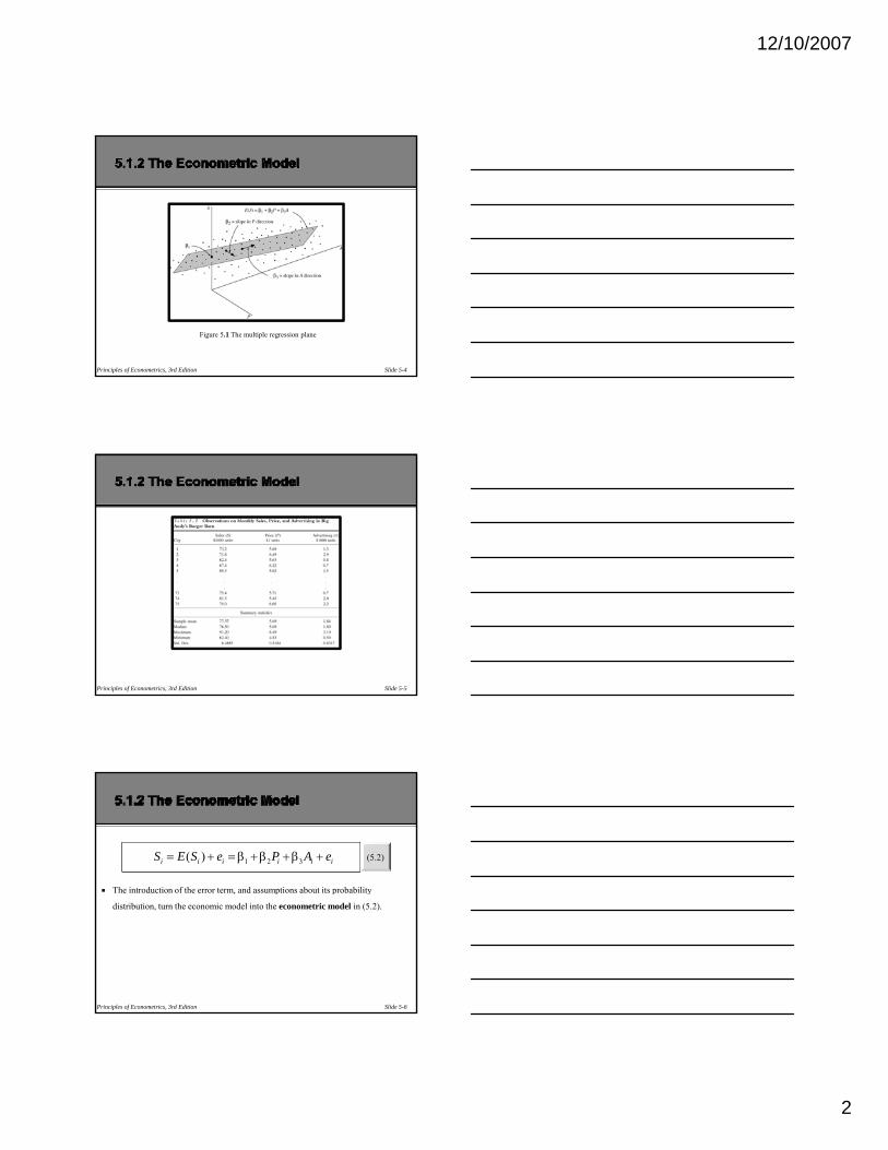
Figure 5.1 The multiple regression plane



The introduction of the error term, and assumptions about its probability

(5.2)1 2 3( )i i i i i iS E S e P A e= + = β +β +β +

, p p y

distribution, turn the economic model into the econometric model in (5.2).


12/10/2007

3

(5.3)1 2 2 3 3i i i K iK iy x x x e= β +β +β + +β +

( ) ( )E EΔ ∂


( ) ( )other 's held constant

kk kx

E y E yx x

Δ ∂β = =

Δ ∂

(5.4)1 2 2 3 3i i iy x x e= β +β +β +

1.

Each random error has a probability distribution with zero mean. Some errors will

( ) 0iE e =

be positive, some will be negative; over a large number of observations they will

average out to zero.


2.

Each random error has a probability distribution with variance σ2. The variance σ2

2var( )ie = σ

is an unknown parameter and it measures the uncertainty in the statistical model. It

is the same for each observation, so that for no observations will the model

uncertainty be more, or less, nor is it directly related to any economic variable.

Errors with this property are said to be homoskedastic.


12/10/2007

4

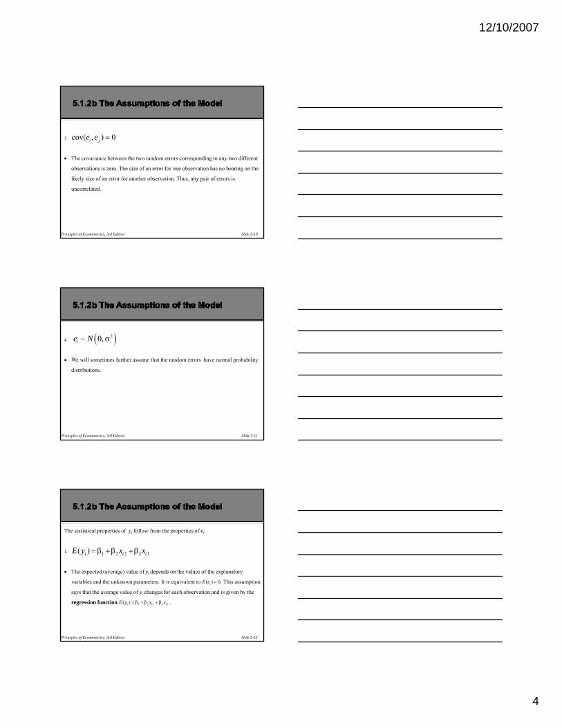
3.

The covariance between the two random errors corresponding to any two different

cov( , ) 0i je e =

observations is zero. The size of an error for one observation has no bearing on the

likely size of an error for another observation. Thus, any pair of errors is

uncorrelated.


4.

We will sometimes further assume that the random errors have normal probability

( )2~ 0,ie N σ

distributions.


The statistical properties of yi follow from the properties of ei.

1. 1 2 2 3 3( )i i iE y x x= β +β +β

The expected (average) value of yi depends on the values of the explanatory

variables and the unknown parameters. It is equivalent to . This assumption

says that the average value of yi changes for each observation and is given by the

regression function .


( ) 0iE e =

1 2 2 3 3( )i i iE y x x= β +β +β

12/10/2007

5

2.

The variance of the probability distribution of yi does not change with each

2var( ) var( )i iy e= = σ

observation. Some observations on yi are not more likely to be further from the

regression function than others.


3.

Any two observations on the dependent variable are uncorrelated. For example, if

cov( , ) cov( , ) 0i j i jy y e e= =

one observation is above E(yi), a subsequent observation is not more or less likely

to be above E(yi).


4.

We sometimes will assume that the values of yi are normally distributed about their

21 2 2 3 3~ ( ),i i iy N x x⎡ ⎤β +β +β σ⎣ ⎦

mean. This is equivalent to assuming that .


( )2~ 0,ie N σ

12/10/2007

6

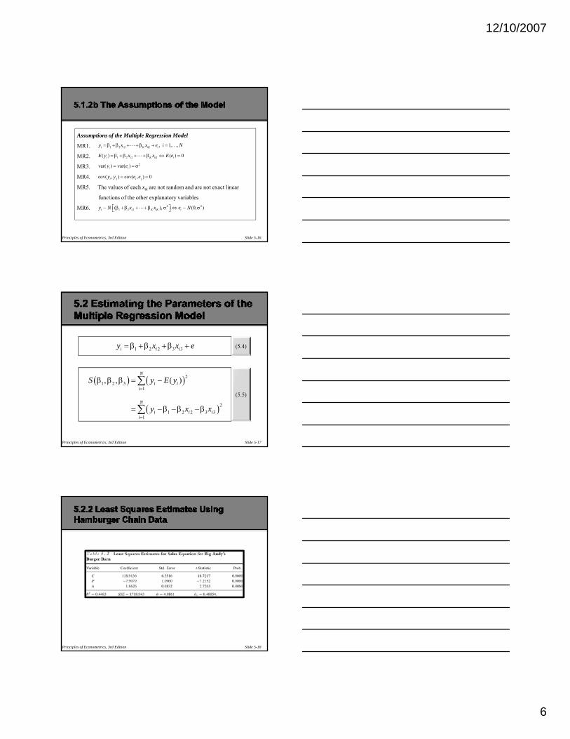
Assumptions of the Multiple Regression Model

MR1.

MR2.

MR3

1 2 2 , 1, ,i i K iK iy x x e i N= β +β + +β + = …

1 2 2( ) ( ) 0i i K iK iE y x x E e= β +β + +β ⇔ =

2( ) ( )


MR3.

MR4.

MR5. The values of each xtk are not random and are not exact linear

functions of the other explanatory variables

MR6.

2var( ) var( )i iy e= = σ

cov( , ) cov( , ) 0i j i jy y e e= =

2 21 2 2~ ( ), ~ (0, )i i K iK iy N x x e N⎡ ⎤β +β + +β σ ⇔ σ⎣ ⎦

(5.4)1 2 2 3 3i i iy x x e= β +β +β +


(5.5)

( ) ( )

( )

21 2 3

1

21 2 2 3 3

1

, , ( )N

i ii

N

i i ii

S y E y

y x x

=

=

β β β = −

= −β −β −β

∑

∑


12/10/2007

7

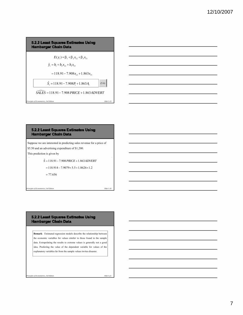
1 2 2 3 3( )i i iE y x x= β +β +β

1 2 2 3 3î i iy b b x b x= + +


(5.6)

2 3118.91 7.908 1.863i ix x= − +

ˆ 118.91 7.908 1.863i i iS P A= − +

118.91 7.908 1.863SALES PRICE ADVERT= − +

Suppose we are interested in predicting sales revenue for a price of

$5.50 and an advertising expenditure of $1,200.

This prediction is given by


ˆ 118.91 7.908 1.863

118.914 7.9079 5.5 1.8626 1.2

77.656

S PRICE ADVERT= − +

= − × + ×

=

Remark: Estimated regression models describe the relationship between

the economic variables for values similar to those found in the sample

data. Extrapolating the results to extreme values is generally not a good


idea. Predicting the value of the dependent variable for values of the

explanatory variables far from the sample values invites disaster.

12/10/2007

8

2 2var( ) ( )i ie E eσ = =

( )1 2 2 3 3ˆ î i i i i ie y y y b b x b x= − = − + +


(5.7)

2

2 1ˆ

ˆ

N

ii

e

N K=σ =−

∑

752

2 1ˆ

1718.943ˆ 23.87475 3

ii

e

N K=σ = = =− −

∑


2

1ˆ 1718.943

N

ii

SSE e=

= =∑

ˆ 23.874 4.8861σ = =

The Gauss-Markov Theorem: For the multiple

regression model, if assumptions MR1-MR5


listed at the beginning of the Chapter hold, then

the least squares estimators are the Best Linear

Unbiased Estimators (BLUE) of the parameters.

12/10/2007

9

(5.8)

2

22 2

23 2 21

var( )(1 ) ( )

N

ii

br x x

=

σ=

− −∑


(5.9)

1i=

2 2 3 323 2 2

2 2 3 3

( )( )( ) ( )

i i

i i

x x x xrx x x x

− −=

− −∑∑ ∑

1. Larger error variances σ2 lead to larger variances of the least squares estimators.

2. Larger sample sizes N imply smaller variances of the least squares estimators.

3. More variation in an explanatory variable around its mean, leads to a smaller variance of the least squares estimator.

4. A larger correlation between x2 and x3 leads to a larger variance of b2.


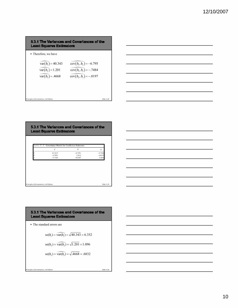
The covariance matrix for K=3 is

( )( ) ( ) ( )

( ) ( ) ( )( ) ( ) ( )

1 1 2 1 3

1 2 3 1 2 2 2 3

var cov , cov ,cov , , cov , var cov ,

cov cov var

b b b b bb b b b b b b b

b b b b b

⎡ ⎤⎢ ⎥= ⎢ ⎥⎢ ⎥⎣ ⎦

The estimated variances and covariances in the example are


(5.10)

( ) ( ) ( )1 3 2 3 3cov , cov , varb b b b b⎢ ⎥⎣ ⎦

( )1 2 3

40.343 6.795 .7484cov , , 6.795 1.201 .0197

.7484 .0197 .4668b b b

− −⎡ ⎤⎢ ⎥= − −⎢ ⎥⎢ ⎥− −⎣ ⎦

12/10/2007

10

Therefore, we have

( ) ( )( ) ( )

1 1 2var 40.343 cov , 6.795b b b

b b b

= = −


( ) ( )( ) ( )

2 1 3

3 2 3

var 1.201 cov , .7484

var .4668 cov , .0197

b b b

b b b

= = −

= = −


The standard errors are

1 1se( ) var( ) 40.343 6.352b b= = =


2 2

3 3

se( ) var( ) 1.201 1.096

se( ) var( ) .4668 .6832

b b

b b

= = =

= = =

12/10/2007

11

1 2 2 3 3i i i K iK iy x x x e= β +β +β + +β +

2 2~ ( ) ~ (0 )y N x x e N⎡ ⎤β +β + +β σ ⇔ σ⎣ ⎦


1 2 2( ), (0, )i i K iK iy N x x e N⎡ ⎤β +β + +β σ ⇔ σ⎣ ⎦

( )~ , vark k kb N b⎡β ⎤⎣ ⎦

(5.11)( )

( )~ 0,1 , for 1, 2, ,var

k k

k

bz N k Kb

−β= = …


(5.12)( )

( )~se( )var

k k k kN K

kk

b bt tbb

−

−β −β= =

(5.13)(72)( ) .95c cP t t t− < < =

b⎛ ⎞−β


(5.15)

(5.14)2 2

2

1.993 1.993 .95se( )bP

b⎛ ⎞β− ≤ ≤ =⎜ ⎟⎝ ⎠

[ ]2 2 2 2 21.993 se( ) 1.993 se( ) .95P b b b b− × ≤ β ≤ + × =

[ ]2 2 2 21.993 se( ), 1.993 se( )b b b b− × + ×

12/10/2007

12

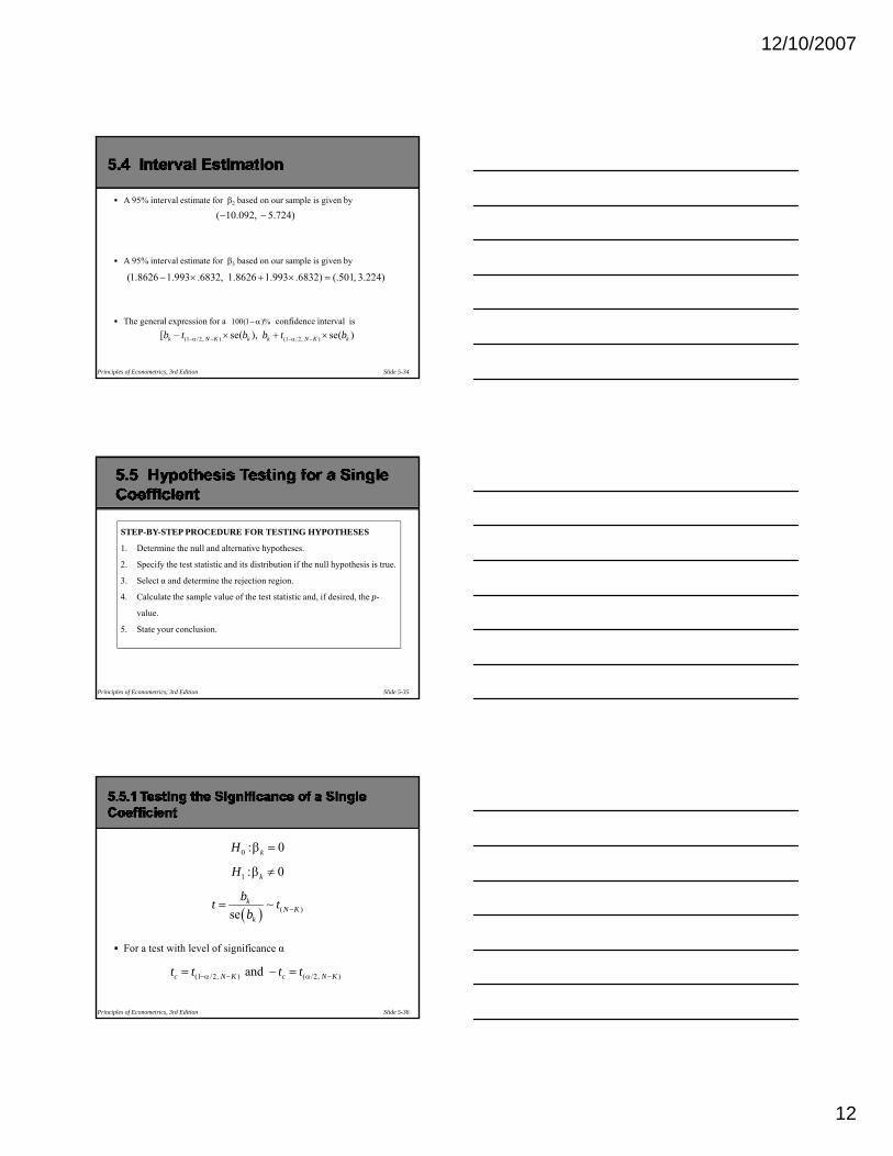
A 95% interval estimate for β2 based on our sample is given by

i l i f β b d l i i b

( 10.092, 5.724)− −

A 95% interval estimate for β3 based on our sample is given by

The general expression for a confidence interval is


(1.8626 1.993 .6832, 1.8626 1.993 .6832) (.501, 3.224)− × + × =

100(1 )%−α

(1 /2, ) (1 /2, )[ se( ), se( )k N K k k N K kb t b b t b−α − −α −− × + ×

STEP-BY-STEP PROCEDURE FOR TESTING HYPOTHESES

1. Determine the null and alternative hypotheses.

2. Specify the test statistic and its distribution if the null hypothesis is true.

3 S l d d i h j i i


3. Select α and determine the rejection region.

4. Calculate the sample value of the test statistic and, if desired, the p-

value.

5. State your conclusion.

0 : 0kH β =

1 : 0kH β ≠

b

For a test with level of significance α


( ) ( )~se

kN K

k

bt tb −=

(1 /2, ) ( /2, ) and c N K c N Kt t t t−α − α −= − =

12/10/2007

13

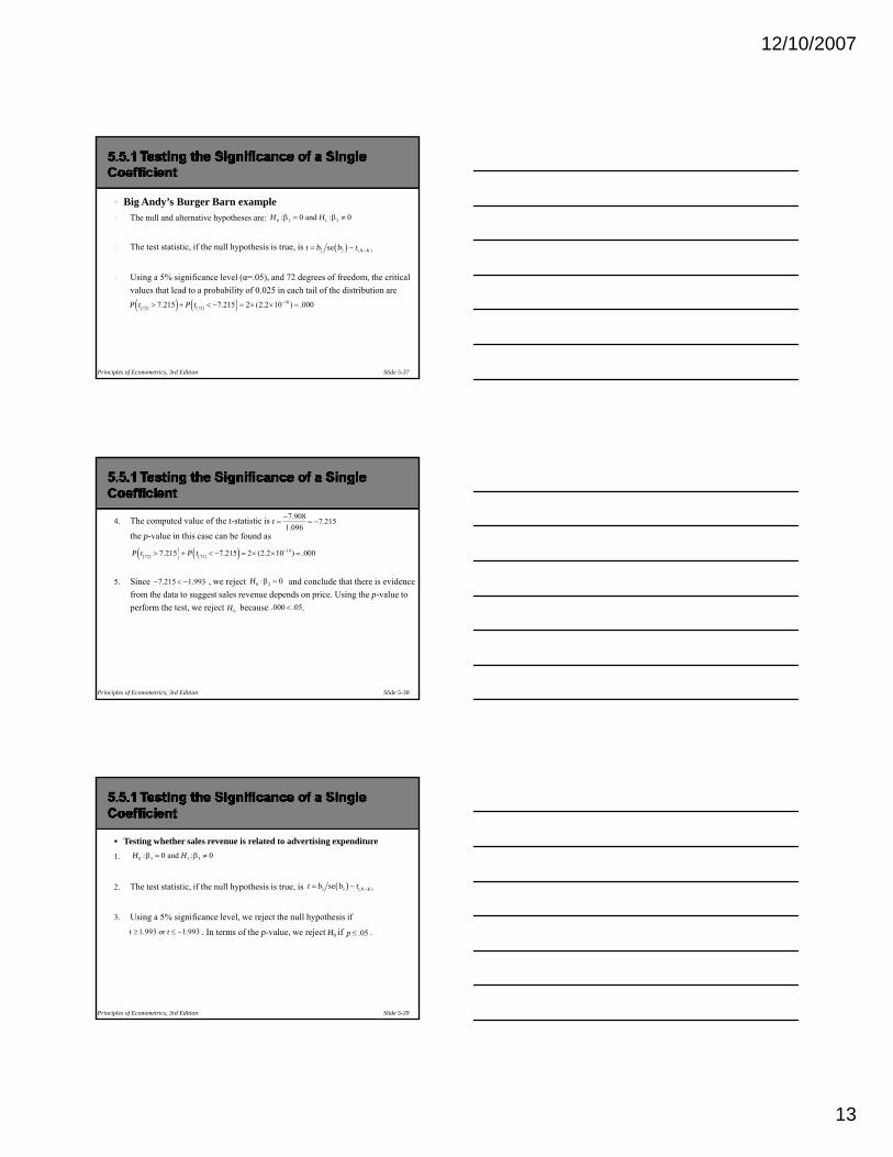
Big Andy’s Burger Barn example 1. The null and alternative hypotheses are:

2. The test statistic, if the null hypothesis is true, is ( )2 2 ( )se ~ N Kt b b t −=

0 2 1 2: 0 and : 0H Hβ = β ≠

3. Using a 5% significance level (α=.05), and 72 degrees of freedom, the critical values that lead to a probability of 0.025 in each tail of the distribution are


( )( ) ( )( ) 1072 727.215 7.215 2 (2.2 10 ) .000P t P t −> + < − = × × =

4. The computed value of the t-statistic is

the p-value in this case can be found as

Si j d l d h h i id0β

7.908 7.2151.096

t −= = −

( )( ) ( )( ) 1072 727.215 7.215 2 (2.2 10 ) .000P t P t −> + < − = × × =

5. Since , we reject and conclude that there is evidence from the data to suggest sales revenue depends on price. Using the p-value to perform the test, we reject because .


7.215 1.993− < − 0 2: 0H β =

0H .000 .05<

Testing whether sales revenue is related to advertising expenditure

1.

2. The test statistic, if the null hypothesis is true, is ( )3 3 ( )se ~ N Kt b b t −=

0 3 1 3: 0 and : 0H Hβ = β ≠

3. Using a 5% significance level, we reject the null hypothesis if

. In terms of the p-value, we reject H0 if .


1.993 or 1.993t t≥ ≤ − .05p ≤

12/10/2007

14

Testing whether sales revenue is related to advertising expenditure

4. The value of the test statistic is ;

the p-value in given by

1.8626 2.726.6832

t = =

( )( ) ( )( )72 722.726 2.726 2 .004 .008P t P t> + < − = × =

5. Because , we reject the null hypothesis; the data support the conjecture that revenue is related to advertising expenditure. Using the p-value we reject .


2.726 1.993>

0 because .008 .05H <

5.5.2a Testing for elastic demand

We wish to know if

: a decrease in price leads to a decrease in sales revenue (demand is price inelastic) or

2 0β ≥

inelastic), or

: a decrease in price leads to an increase in sales revenue (demand is price elastic)


2 0β <

1. (demand is unit elastic or inelastic)

(demand is elastic)0 2: 0H β ≥

1 2: 0H β <

2. To create a test statistic we assume that is true and use

3. At a 5% significance level, we reject


0 2: 0H β =

( )2 2se( ) ~ N Kt b b t −=

0 if 1.666 or if the value .05H t p≤ − − <

12/10/2007

15

4. The value of the test statistic is

The corresponding p-value is

( )2

2

7.908 7.215se 1.096

btb

−= = = −

(72)( 7.215) .000P t < − =

5. . Since , the same conclusion

is reached using the p-value.


0 2Since 7.215 1.666 we reject : 0H− < − β ≥ .000 .05<

5.5.2b Testing Advertising Effectiveness

1.

2. To create a test statistic we assume that is true and use0 3: 1H β =

0 3 1 3: 1 and : 1 H Hβ ≤ β >

1b

3. At a 5% significance level, we reject


0 if 1.666 or if the value .05H t p≥ − − ≤

( )3

3

1 ~se( ) N Kbt t

b −

−=

5.5.2b Testing Advertising Effectiveness

1. The value of the test statistic is

The corresponding p-value is(72)( 1.263) .105P t > =

( )3 3

3

1.8626 1 1.263se .6832bt

b−β −

= = =

p g p

5. . Since .105>.05, the same conclusion is

reached using the p-value.


(72)( )

0Since 1.263<1.666 we do not reject H

12/10/2007

16

( )

( )

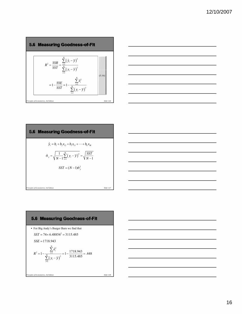
2

2 1

2

ˆN

iiN

i

y ySSRRSST y y

=−

= =−

∑

∑


(5.16)

( )

( )

1

2

1

2

1

ˆ1 1

ii

N

ii

N

ii

y y

eSSESST y y

=

=

=

= − = −−

∑

∑

∑

1 2 2 3 3î i i k iKy b b x b x b x= + + + +

( )21ˆN

y iSSTy yσ = − =∑


( )11 1y i

iy y

N N=− −∑

2ˆ( 1) ySST N= − σ

For Big Andy’s Burger Barn we find that 274 6.48854 3115.485SST = × =

1718.943SSE =


( )

2

2 1

2

1

ˆ1718.9431 1 .4483115.485

N

ii

N

ii

eR

y y=

=

= − = − =−

∑

∑

12/10/2007

17

An alternative measure of goodness-of-fit called the adjusted-R2, is

usually reported by regression programs and it is computed as

2 / ( )1 SSE N KR −


2 ( )1/ ( 1)

RSST N

= −−

If the model does not contain an intercept parameter, then the measure

R2 given in (5.16) is no longer appropriate. The reason it is no longer

appropriate is that, without an intercept term in the model,


( ) ( )2 2 2

1 1 1ˆ ˆ

N N N

i i ii i i

y y y y e= = =

− ≠ − +∑ ∑ ∑

SST SSR SSE≠ +

From this summary we can read off the estimated effects of changes in the

(5.17)2118.9 7.908 1.8626 .448

(se) (6.35) (1.096) (.6832)SALES PRICE ADVERT R= − + =

From this summary we can read off the estimated effects of changes in the explanatory variables on the dependent variable and we can predict values of the dependent variable for given values of the explanatory variables. For the construction of an interval estimate we need the least squares estimate, its standard error, and a critical value from the t-distribution.


12/10/2007

18

BLU estimatorcovariance matrix of least squares estimatorcritical value

estimationleast squares estimatorsmultiple regression model

total sum of squarestwo-tailed test


error variance estimateerror variance estimatorgoodness of fitinterval estimateleast squares estimatesleast squares

one-tailed testp-valueregression coefficientsstandard errorssum of squared errorssum of squares of regressiontesting significance


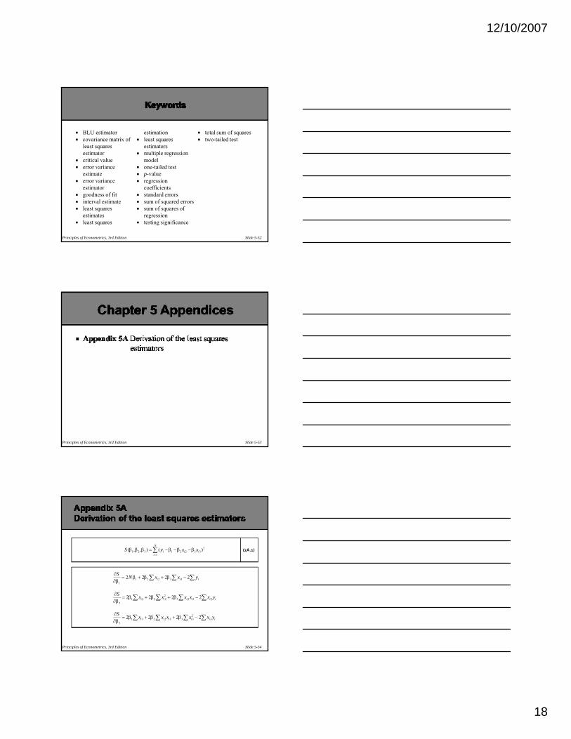
(2A.1)21 2 3 1 2 2 3 3

1( , , ) ( )

N

i i ii

S y x x=

β β β = −β −β −β∑

S∂


1 2 2 3 31

21 2 2 2 3 2 3 2

2

21 3 2 2 3 3 3 3

3

2 2 2 2

2 2 2 2

2 2 2 2

i i i

i i i i i i

i i i i i i

S N x x y

S x x x x x y

S x x x x x y

∂= β + β + β −

∂β

∂= β + β + β −

∂β

∂= β + β + β −

∂β

∑ ∑ ∑

∑ ∑ ∑ ∑

∑ ∑ ∑ ∑

12/10/2007

19

(5A.1)

1 2 2 3 3

22 1 2 2 2 3 3 2

23 1 2 3 2 3 3 3

i i i

i i i i i i

i i i i i i

Nb x b x b y

x b x b x x b x y

x b x x b x b x y

+ + =

+ + =

+ + =

∑ ∑ ∑

∑ ∑ ∑ ∑

∑ ∑ ∑ ∑


2 2 2 3 3 3let , ,i i i i i iy y y x x x x x x∗ ∗ ∗= − = − = −

( )( ) ( )( )( )( ) ( )

1 2 2 3 3

22 3 3 2 3

2 22 22 3 2 3

i i i i i i i

i i i i

b y b x b x

y x x y x x xb

x x x x

∗ ∗ ∗ ∗ ∗ ∗ ∗

∗ ∗ ∗ ∗

= − −

−=

−

∑ ∑ ∑ ∑∑ ∑ ∑


( )( ) ( )( )( )( ) ( )

23 2 2 3 2

3 22 22 3 2 3

i i i i i i i

i i i i

y x x y x x xb

x x x x

∗ ∗ ∗ ∗ ∗ ∗ ∗

∗ ∗ ∗ ∗

−=

−

∑ ∑ ∑ ∑∑ ∑ ∑

Chapter 5 office2007 black and white

Documents