Chapter 4 Consumption, Saving, and Investment Copyright © 2012 Pearson Education Inc.

Chapter 4

Consumption, Saving, and Investment

Copyright © 2012 Pearson Education Inc.

Copyright © 2012 Pearson Education Inc. 4-2

Consumption and Saving Changes in consumers’ willingness

to spend have major implications for the behaviour of the economy. Consumption accounts for about 60%

of total spending. The decision to consume and to save

are closely linked.


Consumption and Saving (continued) Desired consumption (Cd) is the

aggregate quantity of goods and services that household want to consume, given income and other factors.


Consumption and Saving (continued) Desired national saving (Sd) is the

level of national saving that occurs when aggregate consumption is at its desired level.


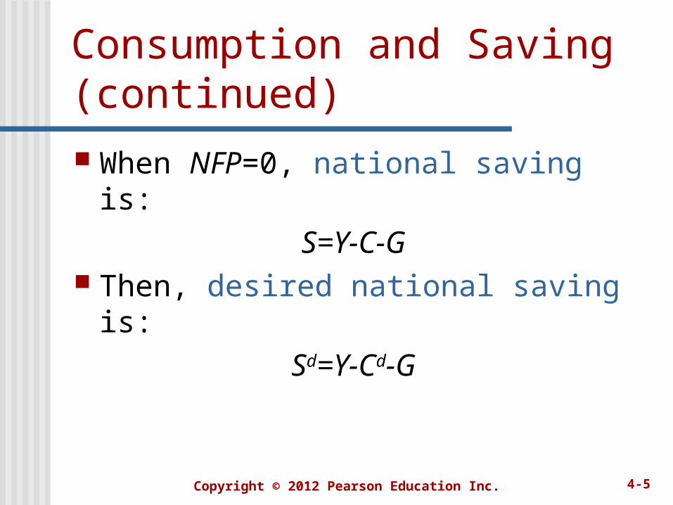
Consumption and Saving (continued) When NFP=0, national saving is:

S=Y-C-G Then, desired national saving is:

Sd=Y-Cd-G


The Consumption and Saving Decision A lender can earn, and a borrower

will have to pay, a real interest rate of r per year.

1 dollars worth of consumption today is equivalent to 1+r dollar’s worth of consumption in the next time period. (assuming inflation = 0)


The Consumption and Saving Decision (continued) The consumption-smoothing

motive is the desire to have a relatively even pattern of consumption over time.

A one-time income bonus is likely to be saved and the income earned on that saving spread over time.


Changes in Current Income Marginal propensity to consume

(MPC) is the fraction of additional current income that is consumed in the current period.

When Y rises by 1: Cd rises by less than 1; Sd rises by the fraction of 1 not spent

on consumption.


Changes in Income and Wealth Current consumption will increase

and current savings will decrease when: expected future income increases,

because of the smoothing motive; wealth increases, because one does

not need to save as much for the future anymore.


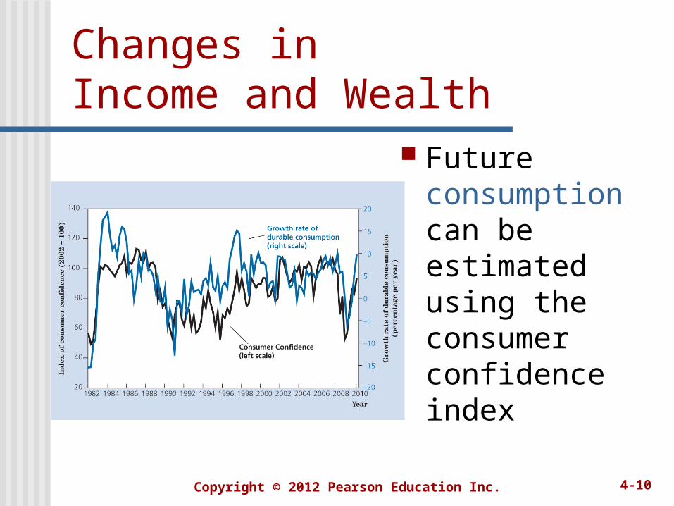
Changes in Income and Wealth

Future consumption can be estimated using the consumer confidence index


Changes in the Real Interest Rate For a lender an increase in r has

two opposite effects: increases the opportunity cost of current

consumption and thus increases current saving (substitution effect);

increases current income from wealth which increases current consumption and decreases in current saving (income effect).


Changes in the Real Interest Rate (continued) For a borrower when r increases

the substitution and income effects both result in increased S.

The empirical evidence is that an increase in r reduces C and increases S, but the effect is not very strong.


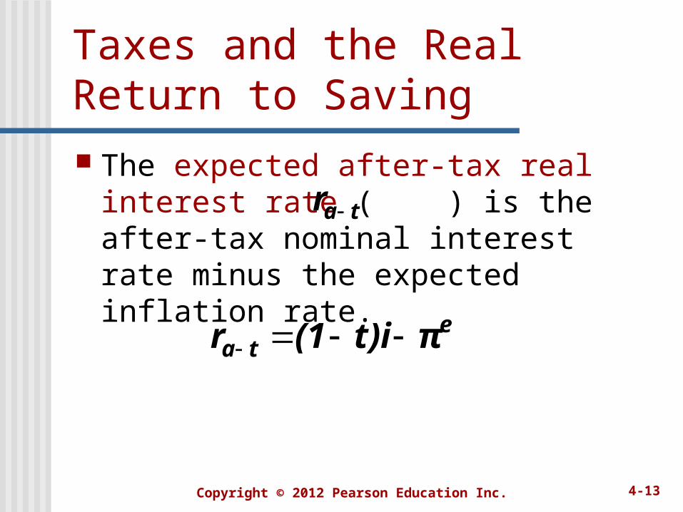
Taxes and the Real Return to Saving The expected after-tax real

interest rate ( ) is the after-tax nominal interest rate minus the expected inflation rate.

tar

eta πt)i(1r


Taxes and the Real Return to Saving (continued) By reducing the tax rate on

interest the government can increase the real rate of return for savers and (possibly) increase the rate of saving in the economy.


Fiscal Policy Let’s make an assumption that the

economy’s aggregate output is given, it is not affected by the changes in fiscal policy.

The government fiscal policy has two major components: the government purchases and taxes.


Government Purchases When the government increases

its purchases temporarily: Cd falls, because higher taxes and

lower income are expected. Sd increases, because Cd falls. Sd falls, because G increases. A total effect on Sd is a fall.


Taxes A government tax cut without

reduction of current spending should: Increase income and, therefore, Cd by

a fraction of the tax cut. Raise expectations of higher taxes

and lower after-tax income in the future.


Taxes (continued) According to the Ricardian

equivalence proposition the positive and the negative effects of the tax cut without reduction of the current spending should exactly cancel.

In reality it may be not so, since many consumers get deceived.


Investment There is a trade-off between the

present and the future. A firm commits its resources to

increasing its capacity to produce and earn profits in the future.


Investment (continued) Investment spending fluctuates

sharply over the business cycle and typically contributes half of the total decline in spending.

Investment plays a crucial role in determining the long-run productive capacity of the economy and its growth.


The Desired Capital Stock Desired capital stock is an amount

of capital that allows a firm to earn the largest expected profit.

The marginal product of capital (MPK) is the firm’s increase in output due to adding a unit of capital (other factors held constant).


The Desired Capital Stock (continued) Managers compare the cost and

benefit of using additional capital, e.g. a new machine.

The firm’s benefit is MPKf – the future MPK.

The firm’s cost is the user cost of capital.


The User Cost of Capital User cost of capital is the expected

real cost of using a unit of capital for a specified period of time.


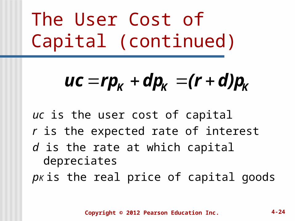
The User Cost of Capital (continued)

uc is the user cost of capitalr is the expected rate of interestd is the rate at which capital depreciatespK is the real price of capital goods

KKK d)p(rdprpuc


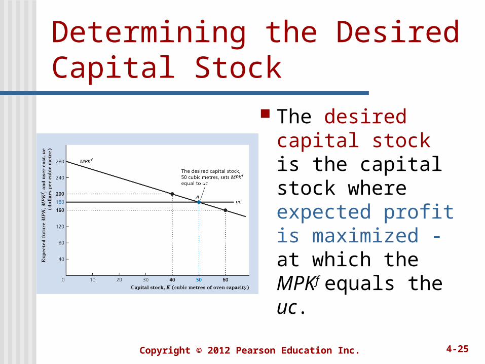
Determining the Desired Capital Stock

The desired capital stock is the capital stock where expected profit is maximized - at which the MPKf equals the uc.


Determining the Desired Capital Stock (continued) The MPKf curve slopes downward

because the marginal product of capital falls as the capital stock increases.

The uc curve does not depend in the amount capital and is a horizontal line.


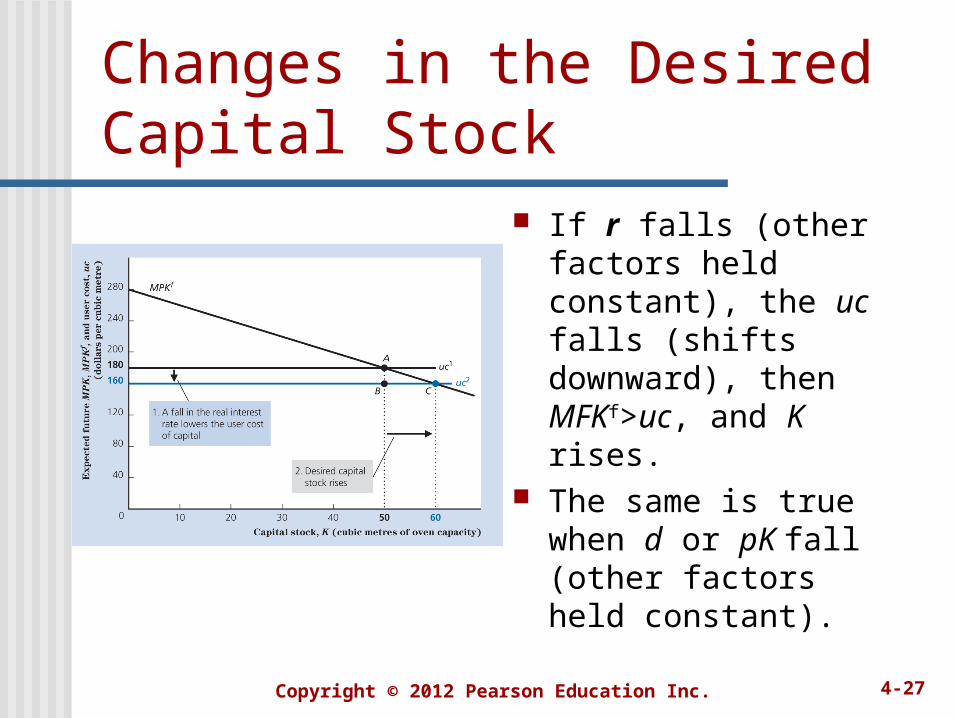
Changes in the Desired Capital Stock

If r falls (other factors held constant), the uc falls (shifts downward), then MFKf>uc, and K rises.

The same is true when d or pK fall (other factors held constant).


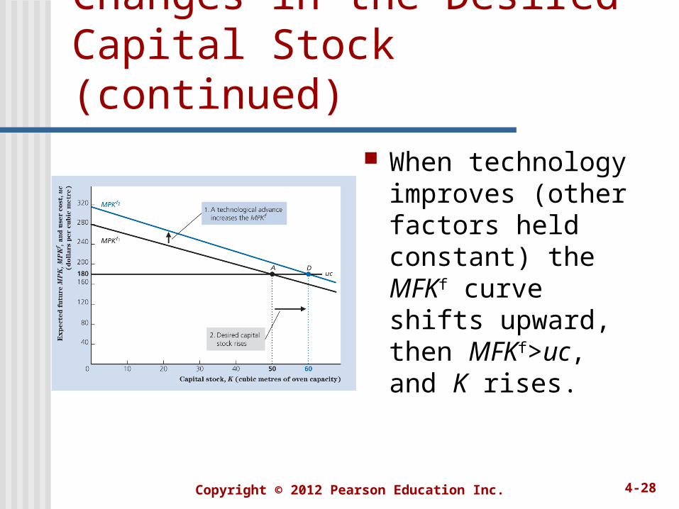
Changes in the Desired Capital Stock (continued)

When technology improves (other factors held constant) the MFKf curve shifts upward, then MFKf>uc, and K rises.


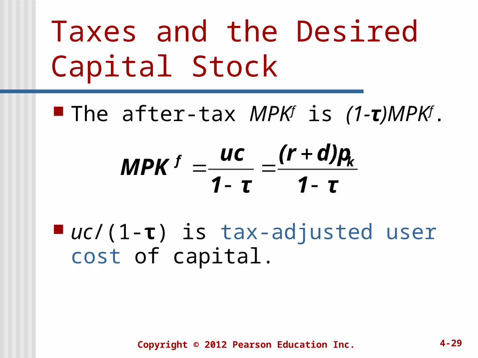
Taxes and the Desired Capital Stock The after-tax MPKf is (1-τ)MPKf.

uc/(1-τ) is tax-adjusted user cost of capital.

τ1

d)p(r

τ1

ucMPK kf


Taxes and the Desired Capital Stock (continued) An increase in the tax rate τ raises

the tax-adjusted user cost and so reduces the desired stock of capital.

The effective tax rate is a single measure of the tax burden on capital.


Investment The capital stock changes:

Gross investment is the total purchase or construction of new capital goods.

Depreciation is the capital wearing out.


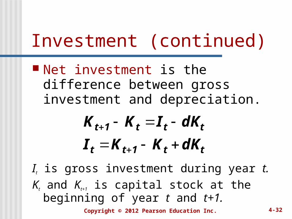
Investment (continued) Net investment is the difference

between gross investment and depreciation.

It is gross investment during year t.Kt and Kt+1 is capital stock at the beginning

of year t and t+1.

tt1tt

ttt1t

dKKKI

dKIKK


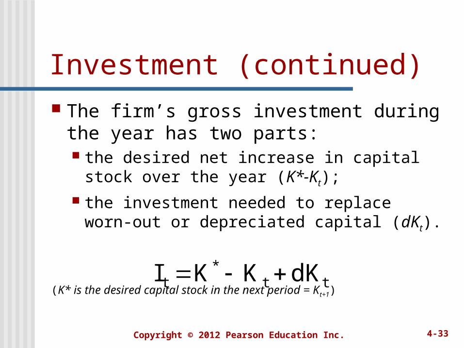
Investment (continued) The firm’s gross investment during

the year has two parts: the desired net increase in capital stock

over the year (K*-Kt); the investment needed to replace worn-

out or depreciated capital (dKt).

(K* is the desired capital stock in the next period = Kt+1)

tt*

t dKKKI


Investment in Inventories A firm’s inventories are unsold

goods, unfinished goods, and raw materials.

Inventory investment is the most volatile component of investment spending.


Investment in Inventories (continued) Residential investment is the

construction of housing or apartment buildings.

A firm’s owner will compare the benefits of keeping higher inventories or renting out apartments and the respective user costs.


Goods Market Equilibrium The real interest rate is the key

economic variable whose adjustments help bring the quantities of goods supplied and demanded into balance.


Goods Market Equilibrium (continued) The goods market equilibrium

condition is:

Y is the quantity of goods supplied by firms.

The right hand side is the aggregate demand for goods.

GICY dd


Goods Market Equilibrium (continued) The income-expenditure identity

for a closed economy (Y=C+I+G) is always satisfied.

The goods market is in equilibrium when desired national saving equals desired investment (Sd=Id), since Sd=Y-Cd-G.


The Saving-Investment Diagram The saving curve, S, is upward

sloping. A higher real interest rate raises desired national savings.

The investment curve, I, is downward sloping. A higher interest rate increases the user cost of capital and, thus, reduces investment.


The Saving-Investment Diagram (continued)

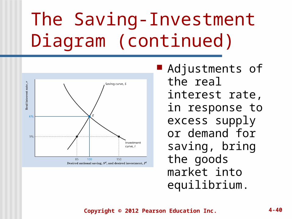
Adjustments of the real interest rate, in response to excess supply or demand for saving, bring the goods market into equilibrium.


The Saving-Investment Diagram (Continued) Goods market equilibrium:

Cd depends on r because a higher r raises Sd.

Id depends on r because a higher r raises uc, which lowers Id.

Adjustments of r eliminate excess supply or demand for saving.


Shifts of theSaving Curve The saving curve shifters are all

factors, excluding the real interest rate, which affect national saving.


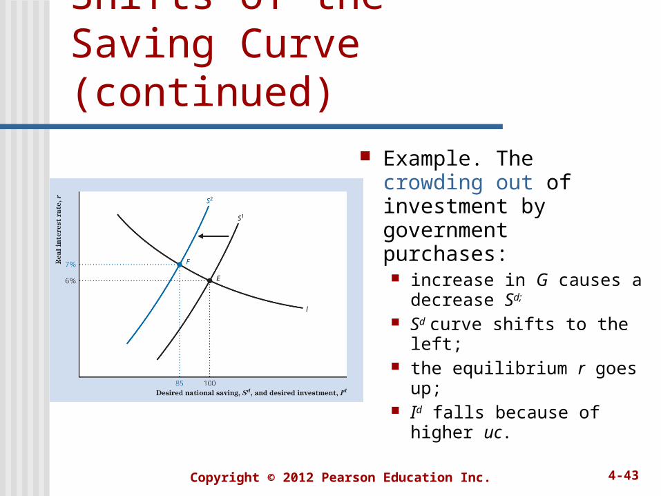
Shifts of theSaving Curve (continued)

Example. The crowding out of investment by government purchases: increase in G causes a

decrease Sd; Sd curve shifts to the

left; the equilibrium r goes

up; Id falls because of higher

uc.


Shifts of theInvestment Curve The investment curve shifters are

all the factors which affect investment, excluding the real interest rate (it determines the movement along the curve).


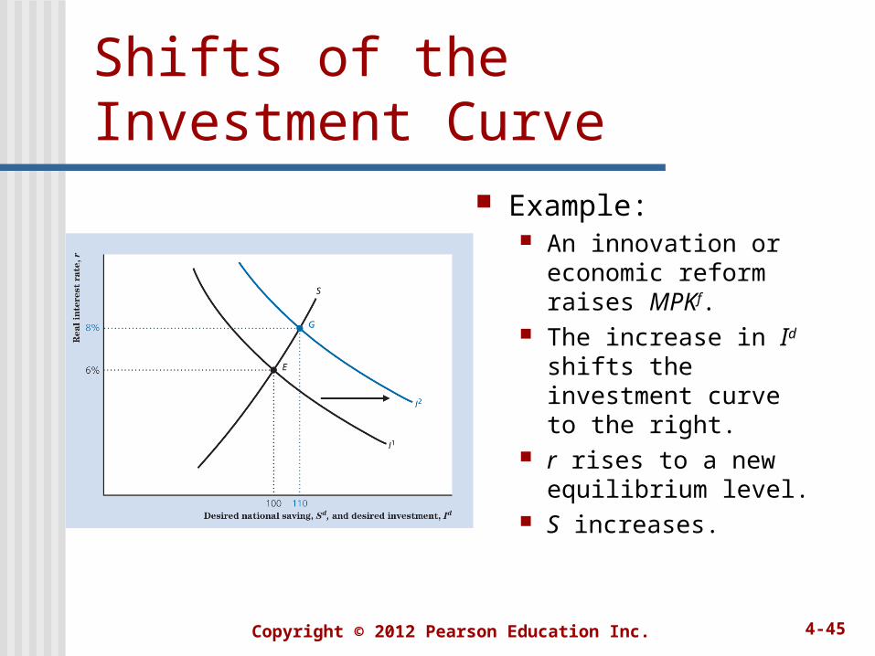
Shifts of theInvestment Curve

Example: An innovation or

economic reform raises MPKf.

The increase in Id shifts the investment curve to the right.

r rises to a new equilibrium level.

S increases.

Chapter 4 Consumption, Saving, and Investment Copyright © 2012 Pearson Education Inc.

Documents

pearson education

wealth current consumption

aggregate consumption

pattern of consumption

consumption accounts

current saving income

wealth future consumption

consumptionsmoothing