Chapter 4 Consumption, Saving, and Investment. Copyright © 2005 Pearson Addison-Wesley. All rights reserved. 4-2 Goals of Chapter 4 Examine the factors.

Chapter 4

Consumption, Saving, and Investment

Copyright © 2005 Pearson Addison-Wesley. All rights reserved. 4-2

Goals of Chapter 4

Examine the factors that underlie economywide demand for goods and services

Assumes closed economy (for now) Focuses on consumption and investment Equivalent to studying saving and capital

formation Examines trade-off of present vs. future Goods market equilibrium when desired saving

equals desired investment Real interest rate plays key role in bringing goods

market to equilibrium


4.1 Consumption and Saving

The importance of consumption and savingDesired consumption: consumption amount desired by

householdsDesired national saving: level of national saving when

consumption is at its desired level, Sd = Y - Cd - G (4.1) The consumption and saving decision of an individual

A person can consume less than current income (saving is positive)

A person can consume more than current income (saving is negative)

Trade-off between current consumption and future consumptionThe price of 1 unit of current consumption is 1 + r units of

future consumption, where r is the real interest rateConsumption-smoothing motive: the desire to have a

relatively even pattern of consumption over time



Effect of changes in current incomeIncrease in current income: both consumption

and saving increase (vice versa for decrease in current income)

Marginal propensity to consume (MPC) = fraction of additional current income consumed in current period; between 0 and 1

Aggregate level: When current income (Y) rises, Cd rises, but not by as much as Y, so Sd rises


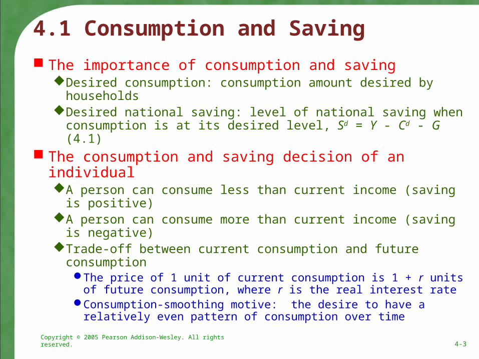
Figure 4.1(a) The index of consumer sentiment, January 1987–December 1994


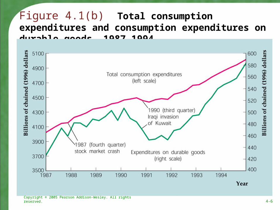
Figure 4.1(b) Total consumption expenditures and consumption expenditures on durable goods, 1987–1994



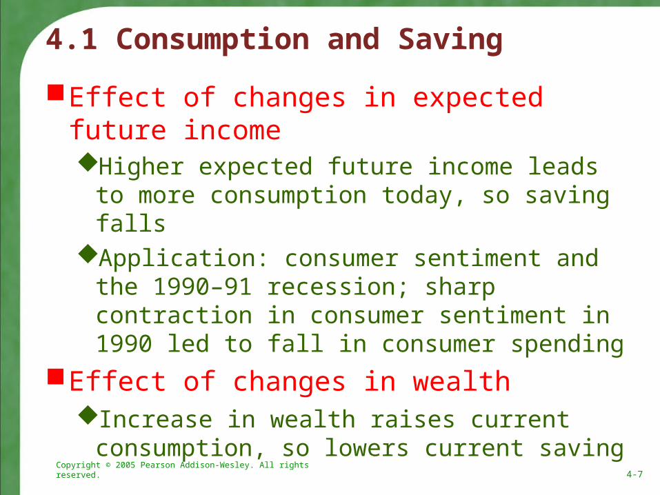
Effect of changes in expected future incomeHigher expected future income leads to more

consumption today, so saving fallsApplication: consumer sentiment and the

1990–91 recession; sharp contraction in consumer sentiment in 1990 led to fall in consumer spending

Effect of changes in wealthIncrease in wealth raises current consumption,

so lowers current saving



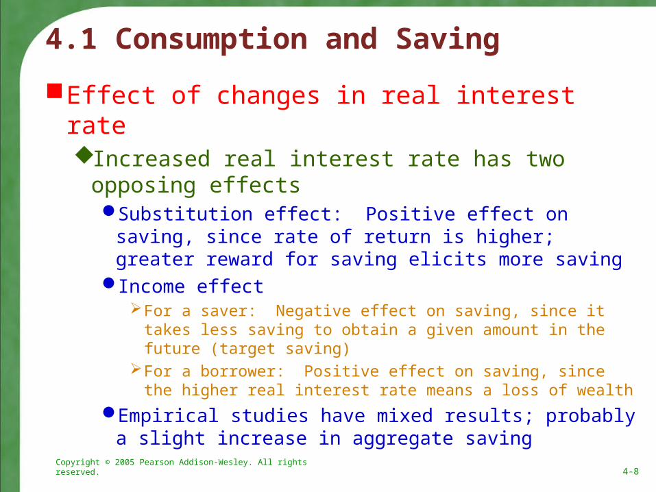
Effect of changes in real interest rateIncreased real interest rate has two opposing

effectsSubstitution effect: Positive effect on saving, since

rate of return is higher; greater reward for saving elicits more saving

Income effectFor a saver: Negative effect on saving, since it takes less

saving to obtain a given amount in the future (target saving)

For a borrower: Positive effect on saving, since the higher real interest rate means a loss of wealth

Empirical studies have mixed results; probably a slight increase in aggregate saving



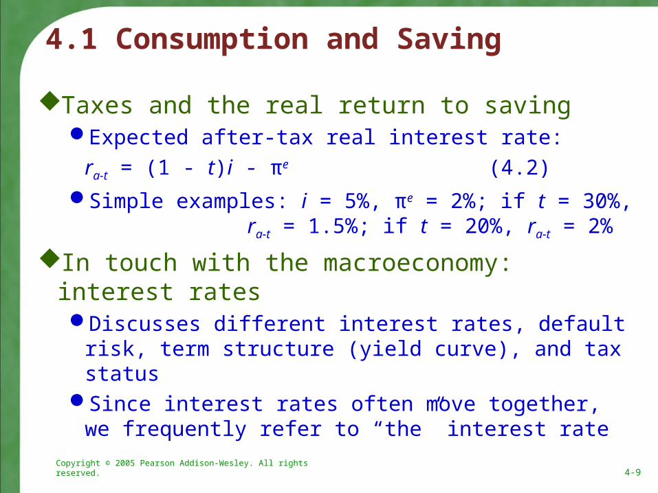
Taxes and the real return to savingExpected after-tax real interest rate:

ra-t = (1 - t)i - πe (4.2)

Simple examples: i = 5%, πe = 2%; if t = 30%, ra-t = 1.5%; if t = 20%, ra-t = 2%

In touch with the macroeconomy: interest ratesDiscusses different interest rates, default risk, term

structure (yield curve), and tax statusSince interest rates often move together, we frequently

refer to “the” interest rate


Table 4.1 Calculating After-Tax Interest Rates



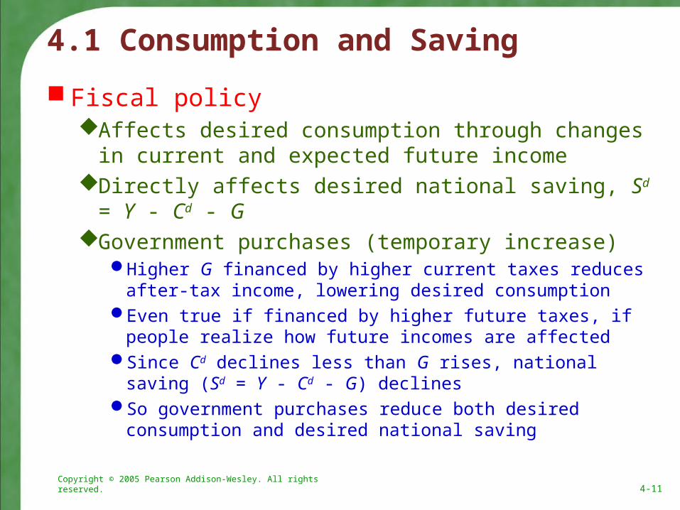
Fiscal policyAffects desired consumption through changes in

current and expected future incomeDirectly affects desired national saving, Sd = Y - Cd - GGovernment purchases (temporary increase)

Higher G financed by higher current taxes reduces after-tax income, lowering desired consumption

Even true if financed by higher future taxes, if people realize how future incomes are affected

Since Cd declines less than G rises, national saving (Sd = Y - Cd - G) declines

So government purchases reduce both desired consumption and desired national saving



Taxes Lump-sum tax cut today, financed by higher future

taxesDecline in future income may offset increase in

current income; desired consumption could rise or fall

Ricardian equivalence proposition If future income loss exactly offsets current income gain,

no change in consumptionTax change affects only the timing of taxes, not their

ultimate amount (present value) In practice, people may not see that future taxes will rise if

taxes are cut today; then a tax cut leads to increased desired consumption and reduced desired national saving




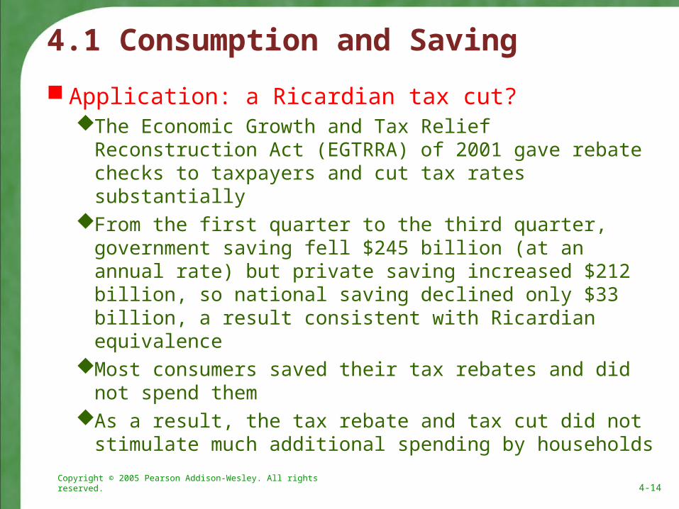
Application: a Ricardian tax cut?The Economic Growth and Tax Relief Reconstruction

Act (EGTRRA) of 2001 gave rebate checks to taxpayers and cut tax rates substantially

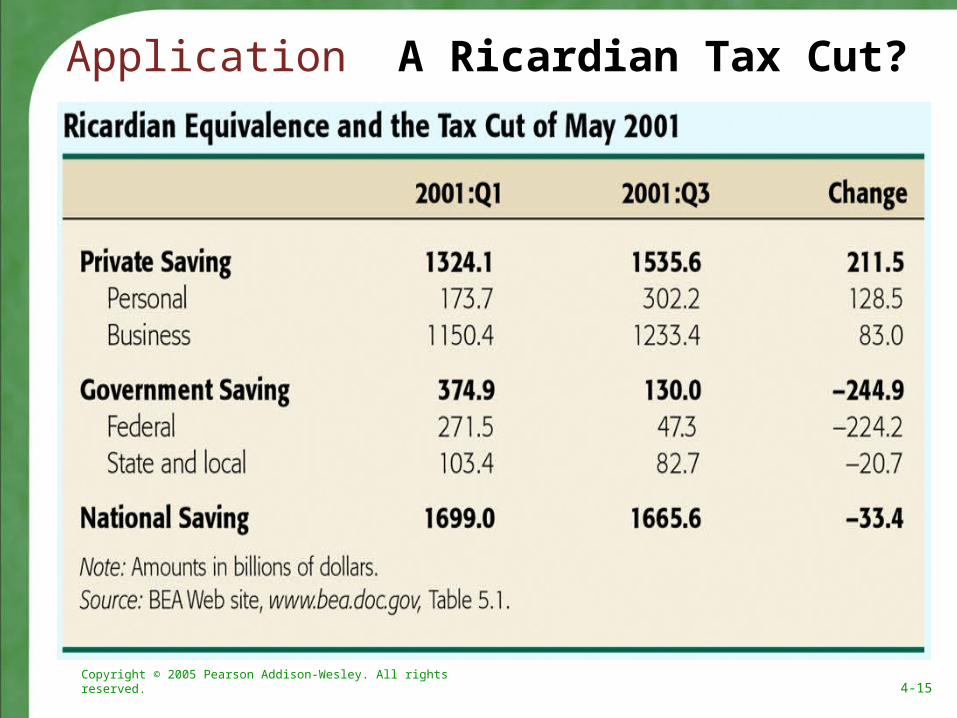
From the first quarter to the third quarter, government saving fell $245 billion (at an annual rate) but private saving increased $212 billion, so national saving declined only $33 billion, a result consistent with Ricardian equivalence

Most consumers saved their tax rebates and did not spend them

As a result, the tax rebate and tax cut did not stimulate much additional spending by households


Application A Ricardian Tax Cut?


4.2 Investment

Why is investment important?Investment fluctuates sharply over the business cycle,

so we need to understand investment to understand the business cycle

Investment plays a crucial role in economic growth The desired capital stock

Desired capital stock is the amount of capital that allows firms to earn the largest expected profit

Desired capital stock depends on costs and benefits of additional capital

Since investment becomes capital stock with a lag, the benefit of investment is the future marginal product of capital (MPKf)


4.2 Investment

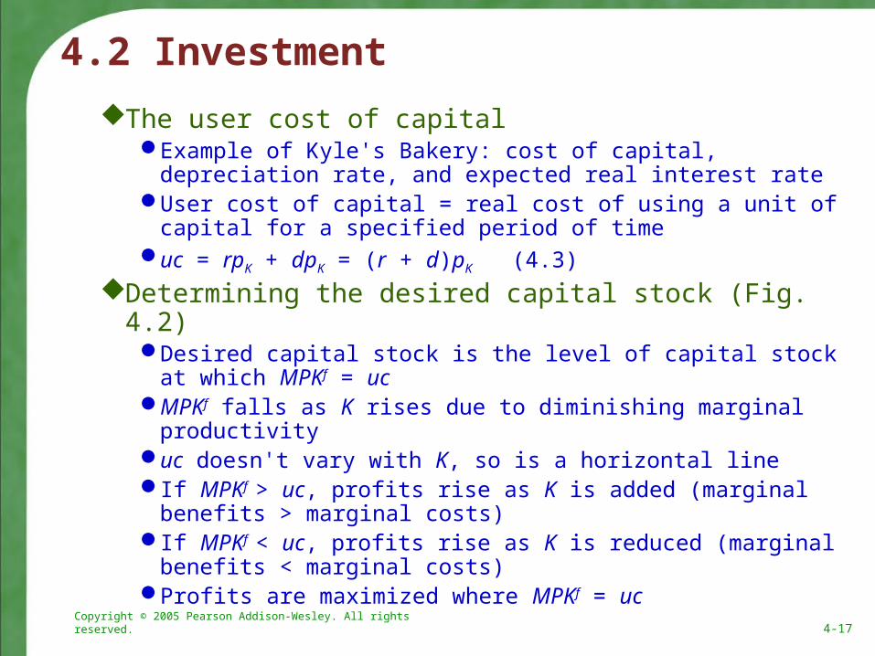
The user cost of capitalExample of Kyle's Bakery: cost of capital, depreciation rate,

and expected real interest rateUser cost of capital = real cost of using a unit of capital for a

specified period of timeuc = rpK + dpK = (r + d)pK (4.3)

Determining the desired capital stock (Fig. 4.2)Desired capital stock is the level of capital stock at which MPKf

= ucMPKf falls as K rises due to diminishing marginal productivityuc doesn't vary with K, so is a horizontal lineIf MPKf > uc, profits rise as K is added (marginal benefits >

marginal costs)If MPKf < uc, profits rise as K is reduced (marginal benefits <

marginal costs)Profits are maximized where MPKf = uc


Figure 4.2 Determination of the desired capital stock


4.2 Investment

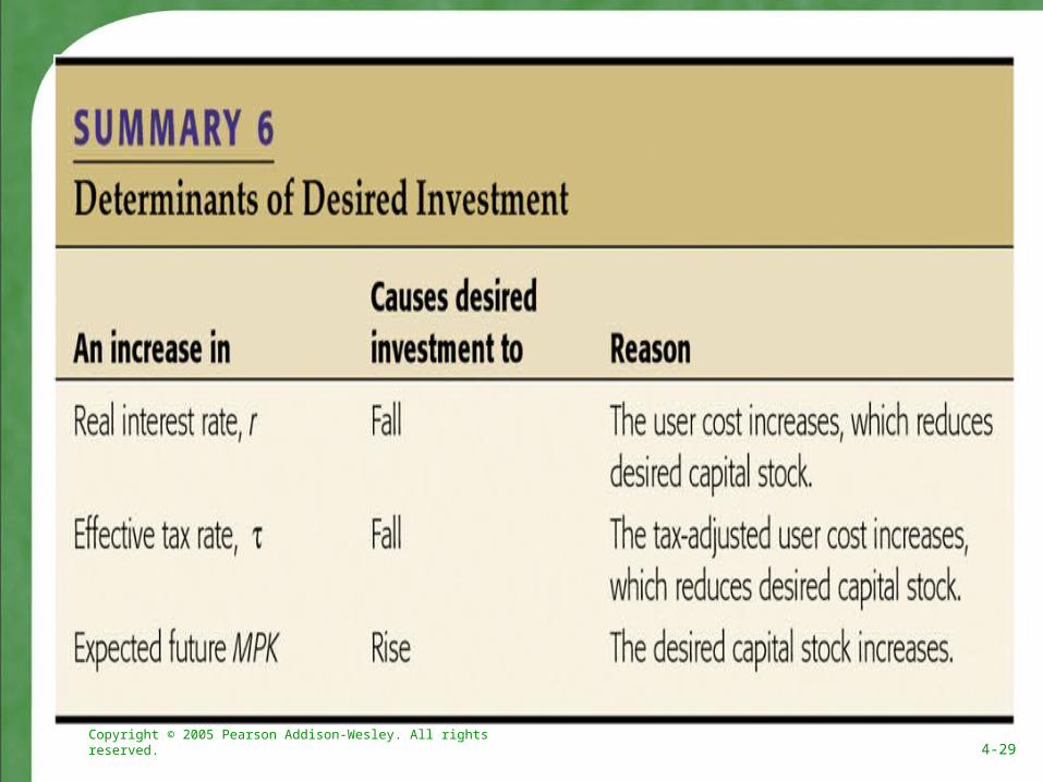
Changes in the desired capital stockFactors that shift the MPKf curve or change the user

cost of capital cause the desired capital stock to change

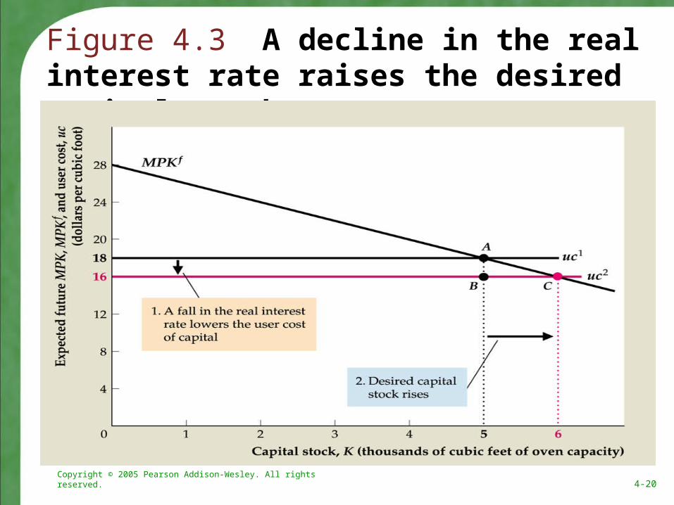
These factors are changes in the real interest rate, depreciation rate, price of capital, or technological changes that affect the MPKf (Fig. 4.3 shows effect of change in uc)

Taxes and the desired capital stockWith taxes, the return to capital is only (1 - τ)MPKf

Setting the return equal to the user cost givesMPKf = uc/(1 - τ) = (r + d)pK/(1 - τ)

Tax-adjusted user cost of capital is uc/(1 - τ)An increase in τ raises the tax-adjusted user cost and reduces

the desired capital stock


Figure 4.3 A decline in the real interest rate raises the desired capital stock


4.2 InvestmentIn reality, there are complications to the tax-adjusted user cost

We assumed that firm revenues were taxed In reality, profits, not revenues, are taxed So depreciation allowances reduce the tax paid by firms,

because they reduce profits Investment tax credits reduce taxes when firms make new

investments Summary measure: the effective tax rate—the tax rate on firm

revenue that would have the same effect on the desired capital stock as do the actual provisions of the tax code

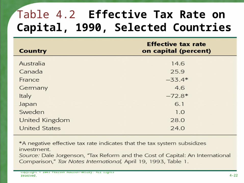
Table 4.2 shows effective tax rates for nine different countries; some are negative, implying a subsidy to capital

Application: measuring the effects of taxes on investment Do changes in the tax rate have a significant effect on investment? A 1994 study by Cummins, Hubbard, and Hassett found that after

major tax reforms, investment responded strongly; elasticity about -0.66 (of investment to user cost of capital)


Table 4.2 Effective Tax Rate on Capital, 1990, Selected Countries


4.2 Investment

Box 4.1: investment and the stock marketFirms change investment in the same direction

as the stock market: Tobin’s q theory of investment

If market value > replacement cost, then firm should invest more

Tobin’s q = capital’s market value divided by its replacement costIf q < 1, don't investIf q > 1, invest more


4.2 Investment

Stock price times number of shares equals firm’s market value, which equals value of firm’s capitalFormula: q = V / (pKK), where V is stock market value of firm,

K is firm’s capital, pK is price of new capitalSo pKK is the replacement cost of firm’s capital stockStock market boom raises V, causing q to rise, increasing

investmentData show general tendency of investment to rise

when stock market rises; but relationship isn’t strong because many other things change at same time

This theory is similar to text discussionHigher MPKf increases future earnings of firm, so V risesA falling real interest rate also raises V as people buy stocks

instead of bondsA decrease in the cost of capital, pK, raises q


Figure 4.4 An increase in the expected future MPK raises the desired capital stock


4.2 Investment

From the desired capital stock to investmentThe capital stock changes from two opposing channels

New capital increases the capital stock; this is gross investmentThe capital stock depreciates, which reduces the capital stockNet investment = gross investment (I) minus depreciation:

Kt+1 - Kt = It - dKt (4.5) , where net investment equals the change in the capital stock

Fig. 4.5 shows gross and net investment for the United States Rewriting (4.5) gives It = Kt+1 - Kt + dKt

If firms can change their capital stocks in one period, then the desired capital stock (K*) = Kt+1, so It = K* - Kt + dKt (4.6)

Thus investment has two parts Desired net increase in the capital stock over the year (K* - Kt) Investment needed to replace depreciated capital (dKt)

Lags and investmentSome capital can be constructed easily, but other capital may take

years to put in placeSo investment needed to reach the desired capital stock may be

spread out over several years


Figure 4.5 Gross and net investment, 1929–2002


4.2 Investment

Investment in inventories and housingMarginal product of capital and user cost also

apply, as with equipment and structures



4.3 Goods Market Equilibrium

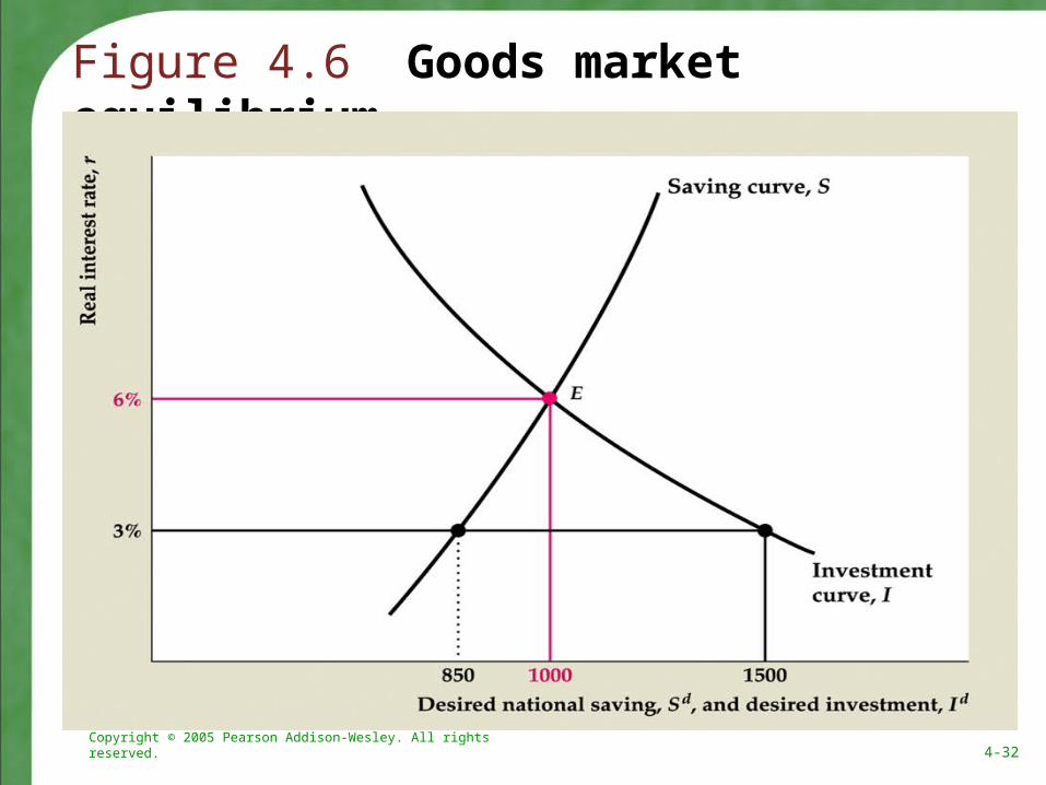
The real interest rate adjusts to bring the goods market into equilibriumgoods market equilibrium condition :

Y = Cd + Id + G (4.7) Differs from income-expenditure identity, as goods

market equilibrium condition need not hold; undesired goods may be produced, so goods market won't be in equilibrium

Alternative representation: since Sd = Y - Cd - G, Sd = Id (4.9)

The saving-investment diagram Plot Sd vs. Id (Key Diagram 3; Fig. 4.6)Equilibrium where Sd = Id

How to reach equilibrium? Adjustment of r


Key Diagram 3 The saving– investment diagram


Figure 4.6 Goods market equilibrium


Table 4.3 Components of Aggregate Demand for Goods (An Example)



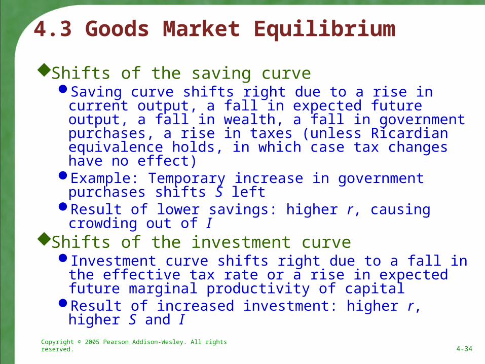
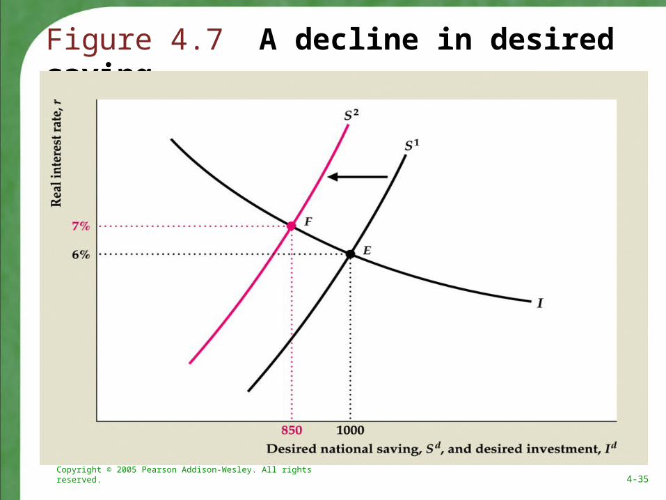
Shifts of the saving curveSaving curve shifts right due to a rise in current output,

a fall in expected future output, a fall in wealth, a fall in government purchases, a rise in taxes (unless Ricardian equivalence holds, in which case tax changes have no effect)

Example: Temporary increase in government purchases shifts S left

Result of lower savings: higher r, causing crowding out of I

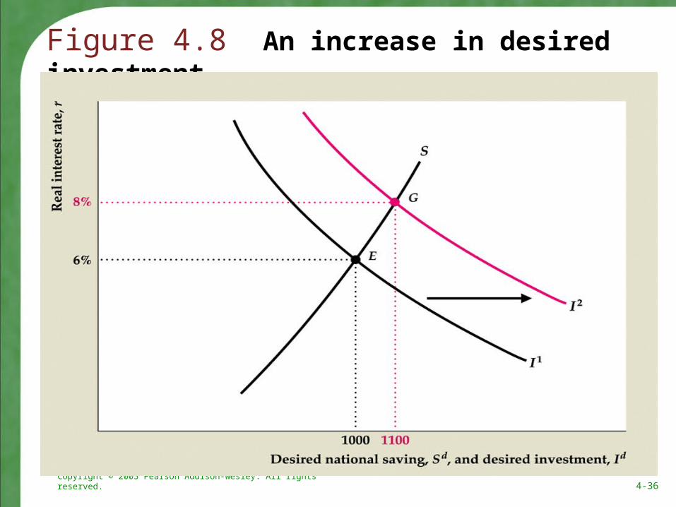
Shifts of the investment curveInvestment curve shifts right due to a fall in the

effective tax rate or a rise in expected future marginal productivity of capital

Result of increased investment: higher r, higher S and I


Figure 4.7 A decline in desired saving


Figure 4.8 An increase in desired investment



Application: Macroeconomic consequences of the boom and bust in stock pricesSharp changes in stock prices affect consumption

spending (a wealth effect) and capital investment (via Tobin’s q)

Consumption and the 1987 crashWhen the stock market crashed in 1987, wealth declined by

about $1 trillionConsumption fell somewhat less than might be expected, and

it wasn’t enough to cause a recessionThere was a temporary decline in confidence about the future,

but it was quickly reversedThe small response may have been because there had been a

large run-up in stock prices between December 1986 and August 1987, so the crash mostly erased this run-up


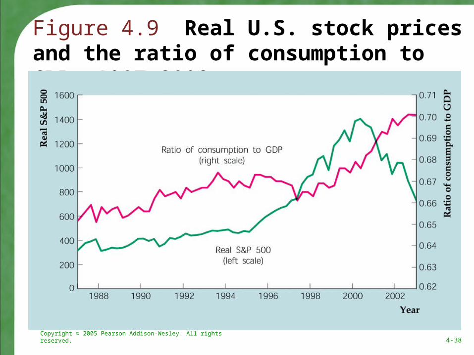
Figure 4.9 Real U.S. stock prices and the ratio of consumption to GDP, 1987–2002



Consumption and the rise in stock market wealth in the 1990sStock prices more than tripled in real terms But consumption was not strongly affected by the runup in

stock pricesConsumption and the decline in stock prices in the

early 2000sIn the early 2000s, wealth in stocks declined by about $5

trillionBut consumption spending increased as a share of GDP in

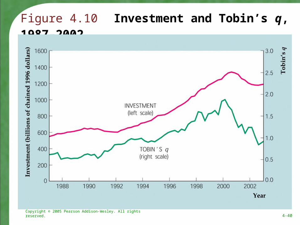
that periodInvestment and Tobin’s q

Investment and Tobin’s q were not closely correlated following the 1987 crash in stock prices

But the relationship has been tighter in the 1990s and early 2000s, as theory suggests


Figure 4.10 Investment and Tobin’s q, 1987–2002

Appendix 4A

A Formal Model of Consumption and Saving


Appendix 4.A: A Formal Model of Consumption and Saving

How much can the consumer afford? The budget constraint (BC)Current income y; future income yf; initial wealth aChoice variables: af = wealth at beginning of future period; c =

current consumption; cf = future consumptionaf = (y + a - c)(1 + r), so cf = (y + a - c)(1 + r) + yf (4.A.1) the BC

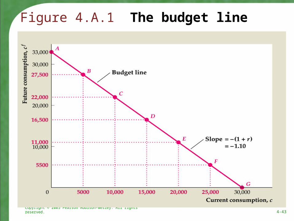
The budget lineGraph budget line in (c, cf) space (Fig. 4.A.1)Slope of line = -(1 + r)

Present valuesPresent value is the value of payments to be made in the future in

terms of today's dollars or goodsExample: At an interest rate of 10%, $12,000 today invested for

one year is worth $13,200 ($12,000 × 1.10); so the present value of $13,200 in one year is $12,000

General formula: Present value = future value / (1 + i), where amounts are in dollar terms and i is the nominal interest rate

Alternatively, if amounts are in real terms, use the real interest rate r instead of the nominal interest rate i


Figure 4.A.1 The budget line


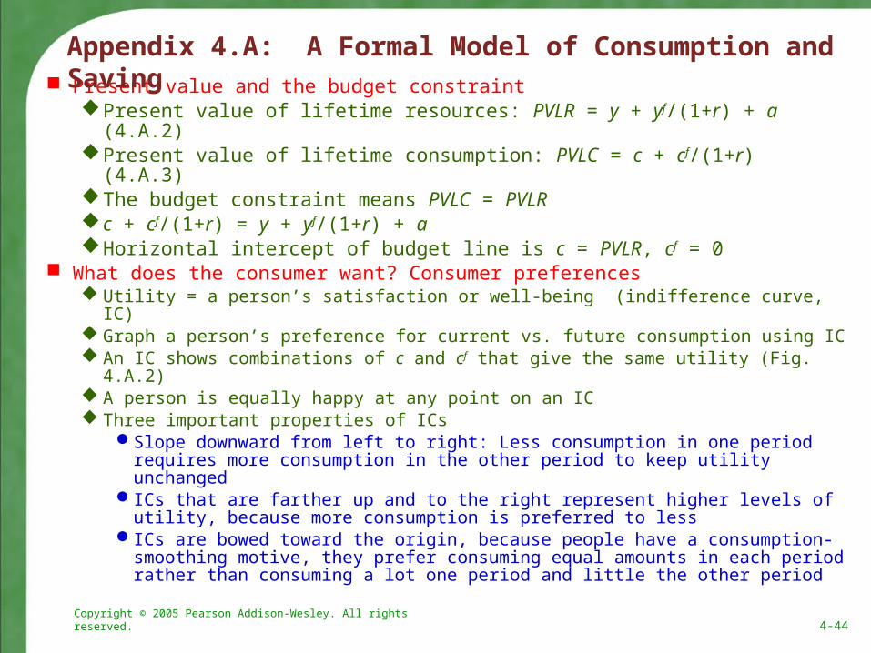
Present value and the budget constraintPresent value of lifetime resources: PVLR = y + yf/(1+r) + a (4.A.2)Present value of lifetime consumption: PVLC = c + cf/(1+r) (4.A.3)The budget constraint means PVLC = PVLRc + cf/(1+r) = y + yf/(1+r) + a Horizontal intercept of budget line is c = PVLR, cf = 0

What does the consumer want? Consumer preferences Utility = a person’s satisfaction or well-being (indifference curve, IC) Graph a person’s preference for current vs. future consumption using IC An IC shows combinations of c and cf that give the same utility (Fig. 4.A.2) A person is equally happy at any point on an IC Three important properties of ICs

Slope downward from left to right: Less consumption in one period requires more consumption in the other period to keep utility unchanged

ICs that are farther up and to the right represent higher levels of utility, because more consumption is preferred to less

ICs are bowed toward the origin, because people have a consumption-smoothing motive, they prefer consuming equal amounts in each period rather than consuming a lot one period and little the other period



Figure 4.A.2 Indifference curves


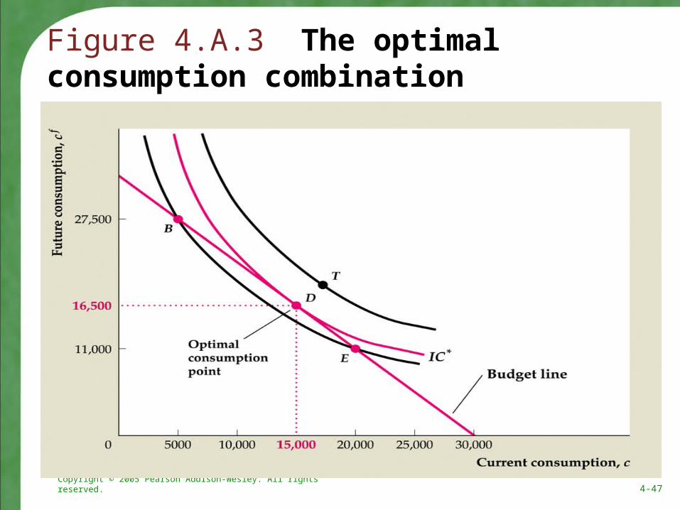
The optimal level of consumption Optimal consumption point is where the budget line is tangent to an IC (Fig.

4.A.3) That’s the highest IC that it’s possible to reach All other points on the budget line are on lower ICs

The Effects of Changes in Income and Wealth on Consumption and Saving The effect on consumption of a change in income (current or future) or

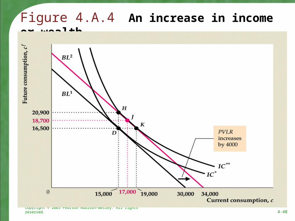
wealth depends only on how the change affects the PVLRAn increase in current income (Fig. 4.A.4)

Increases PVLR, so shifts budget line out parallel to old budget line If there is a consumption-smoothing motive, both current and future

consumption will increase Then both consumption and saving rise because of the rise in current income

An increase in future income Same outward shift in budget line as an increase in current income Again, with consumption smoothing, both current and future consumption

increase Now saving declines, since current income is unchanged and current

consumption increasesAn increase in wealth

Same parallel shift in budget line, so both current and future consumption rise Again, saving declines, since c rises and y is unchanged



Figure 4.A.3 The optimal consumption combination


Figure 4.A.4 An increase in income or wealth


The permanent income theory Different types of changes in income

Temporary increase in income: y rises and yf is unchanged Permanent increase in income: Both y and yf rise

Permanent income increase causes bigger increase in PVLR than a temporary income increase

So current consumption will rise more with a permanent income increase

So saving from a permanent increase in income is less than from a temporary increase in income

This distinction between permanent and temporary income changes was made by Milton Friedman in the 1950s and is known as the permanent income theory

Permanent changes in income lead to much larger changes in consumption

Thus permanent income changes are mostly consumed, while temporary income changes are mostly saved



Consumption and Saving Over Many Periods: The Life-Cycle ModelLife-cycle model was developed by Franco Modigliani and

associates in the 1950sLooks at patterns of income, consumption, and saving over an

individual’s lifetimeTypical consumer’s income and saving pattern shown in Fig. 4.A.5 Real income steadily rises over time until near retirement; at retirement,

income drops sharplyLifetime pattern of consumption is much smoother than the income

pattern In reality, consumption varies somewhat by age For example, when raising children, household consumption is

higher than average The model can easily be modified to handle this and other variations

Saving has the following lifetime pattern Saving is low or negative early in working life Maximum saving occurs when income is highest (ages 50 to 60) Dissaving occurs in retirement



Figure 4.A.5 Life-cycle consumption, income, and saving


Figure 4.A.5 Life-cycle consumption, income, and saving (cont’d)


Bequests and savingWhat effect does a bequest motive (a desire to leave an

inheritance) have on saving?Simply consume less and save more than without a bequest

motive

Ricardian equivalenceWe can use the two-period model to examine Ricardian

equivalenceThe two-period model shows that consumption is changed

only if the PVLR changesSuppose the government reduces taxes by 100 in the current

period, the interest rate is 10%, and taxes will be increased by 110 in the future period

Then the PVLR is unchanged, and thus there is no change in consumption



Excess sensitivity and borrowing constraintsGenerally, theories about consumption, including the

permanent income theory, have been supported by looking at real-world data

But some researchers have found that the data show that the impact of an income or wealth change is different than that implied by a change in the PVLR

There seems to be excess sensitivity of consumption to changes in current income

This could be due to short-sighted behaviorOr it could be due to borrowing constraints

Borrowing constraints mean people can’t borrow as much as they want. Lenders may worry that a consumer won’t pay back the loan, so they won't lend



If a person wouldn’t borrow anyway, the borrowing constraint is said to be nonbinding

But if a person wants to borrow and can’t, the borrowing constraint is binding

A consumer with a binding borrowing constraint spends all income and wealth on consumption

So an increase in income or wealth will be entirely spent on consumption

This causes consumption to be excessively sensitive to current income changes

How prevalent are borrowing constraints? Perhaps 20% to 50% of the U.S. population faces binding borrowing constraints




The Real Interest Rate and the Consumption-Saving Decision The real interest rate and the budget line

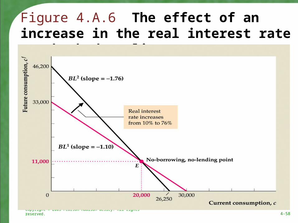
(Fig. 4.A.6)When the real interest rate rises, one point

on the old budget line is also on the new budget line: the no-borrowing, no-lending point

Slope of new budget line is steeper


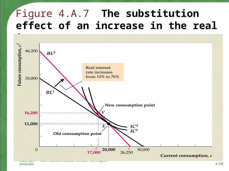
The substitution effectA higher real interest rate makes future consumption

cheaper relative to current consumptionIncreasing future consumption and reducing current

consumption increases savingSuppose a person is at the no-borrowing, no-lending point

when the real interest rate rises (Fig. 4.A.7)An increase in the real interest rate unambiguously

leads the person to increase future consumption and decrease current consumption

The increase in saving, equal to the decrease in current consumption, represents the substitution effect



Figure 4.A.6 The effect of an increase in the real interest rate on the budget line


Figure 4.A.7 The substitution effect of an increase in the real interest rate


The income effectIf a person is planning to consume at the no-

borrowing, no-lending point, then a rise in the real interest rate leads just to a substitution effect

But if a person is planning to consume at a different point than the no-borrowing, no-lending point, there is also an income effect




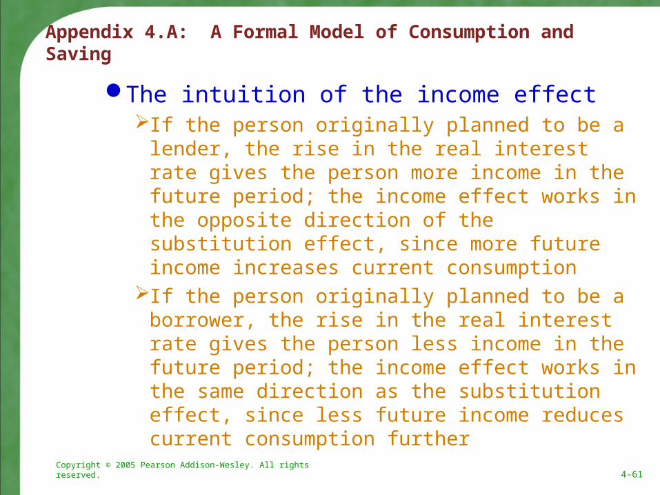
The intuition of the income effectIf the person originally planned to be a lender,

the rise in the real interest rate gives the person more income in the future period; the income effect works in the opposite direction of the substitution effect, since more future income increases current consumption

If the person originally planned to be a borrower, the rise in the real interest rate gives the person less income in the future period; the income effect works in the same direction as the substitution effect, since less future income reduces current consumption further


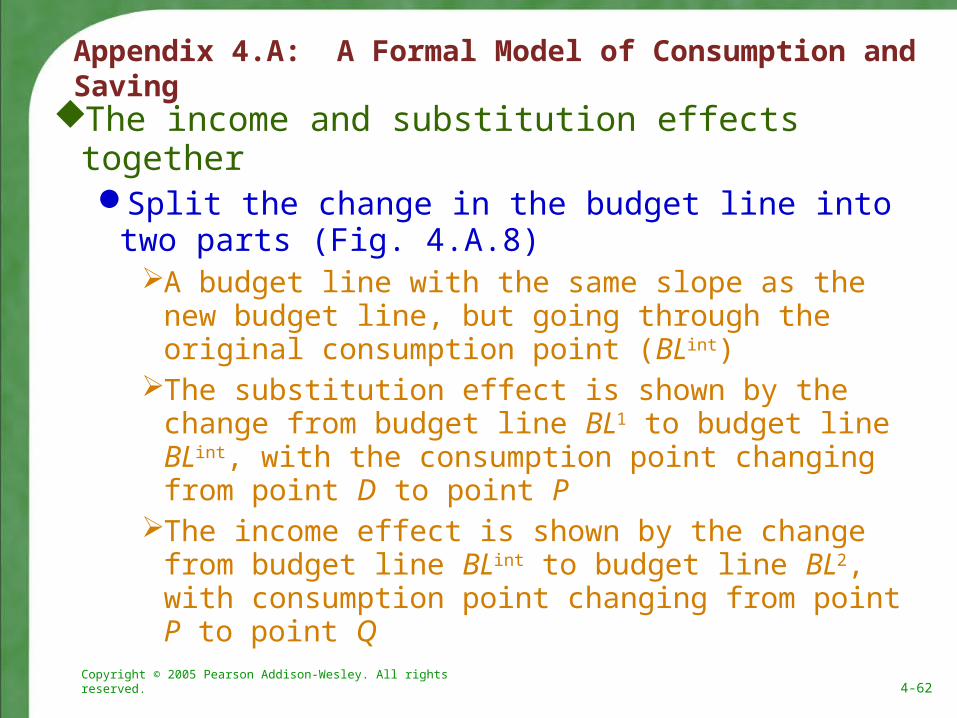
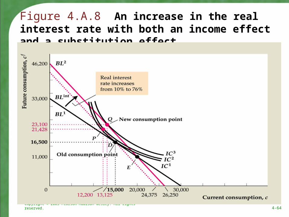
The income and substitution effects togetherSplit the change in the budget line into two parts

(Fig. 4.A.8)A budget line with the same slope as the new budget

line, but going through the original consumption point (BLint)

The substitution effect is shown by the change from budget line BL1 to budget line BLint, with the consumption point changing from point D to point P

The income effect is shown by the change from budget line BLint to budget line BL2, with consumption point changing from point P to point Q




The substitution effect decreases current consumption, but the income effect increases current consumption; so saving may increase or decrease

Both effects increase future consumptionFor a borrower, both effects decrease current

consumption, so saving definitely increases but the effect on future consumption is ambiguous

The effect on aggregate saving of a rise in the real interest rate is ambiguous theoretically

Empirical research suggests that saving increases

But the effect is small


Figure 4.A.8 An increase in the real interest rate with both an income effect and a substitution effect

Chapter 4 Consumption, Saving, and Investment. Copyright © 2005 Pearson Addison-Wesley. All rights reserved. 4-2 Goals of Chapter 4 Examine the factors.

Documents