CHAPTER 2 LITERATURE SURVEY - Shodhgangashodhganga.inflibnet.ac.in/bitstream/10603/8270/11/11_chapter 2.pdf · CHAPTER 2 LITERATURE SURVEY ... "expert" in the category of information

24

CHAPTER 2

LITERATURE SURVEY

2.1 Neural Networks Basics:

An Artificial Neural Network (ANN) is an information processing

paradigm that is inspired by the way biological nervous systems, such as

the brain, process information. The key element of this paradigm is the

novel structure of the information processing system. It is composed of a

large number of highly interconnected processing elements (neurons)

working in unison to solve specific problems. ANNs, like people, learn

by example. An ANN is configured for a specific application, such as

pattern recognition or data classification, through a learning process.

Learning in biological systems involves adjustments to the synaptic

connections that exist between the neurons. This is true of ANNs as well.

2.1.1 Use Neural Networks:

Neural networks, with their remarkable ability to derive meaning

from complicated or imprecise data, can be used to extract patterns and

detect trends that are too complex to be noticed by either humans or other

computer techniques. A trained neural network can be thought of as an

"expert" in the category of information it has been given to analyze. This

expert can then be used to provide projections given new situations of

interest and answer "what if" questions.

2.1.2 Advantages of ANN:

i. Adaptive learning: An ability to learn how to do tasks based on

the data given for training or initial experience.

ii. Self-Organization: An ANN can create its own organization or

representation of the information it receives during learning time.

iii. Real Time Operation: ANN computations may be carried out in

parallel, and special hardware devices are being designed and

manufactured which take advantage of this capability.

25

iv. Fault Tolerance via Redundant Information Coding: Partial

destruction of a network leads to the corresponding degradation of

performance. However, some network capabilities may be retained

even with major network damage.

2.1.3 Neural Networks versus Conventional Computers:

Neural networks take a different approach to problem solving than

that of conventional computers. Conventional computers use an

algorithmic approach i.e. the computer follows a set of instructions in

order to solve a problem. Unless the specific steps that the computer

needs to follow are known the computer cannot solve the problem. That

restricts the problem solving capability of conventional computers to

problems that we already understand and know how to solve. But

computers would be so much more useful if they could do things that we

don't exactly know how to do.

Neural networks process information in a similar way the human

brain does. The network is composed of a large number of highly

interconnected processing elements (neurons) working in parallel to solve

a specific problem. Neural networks learn by example. They cannot be

programmed to perform a specific task. The examples must be selected

carefully otherwise useful time is wasted or even worse the network

might be functioning incorrectly. The disadvantage is that because the

network finds out how to solve the problem by itself, its operation can be

unpredictable.

On the other hand, conventional computers use a cognitive

approach to problem solving; the way the problem is to solved must be

known and stated in small unambiguous instructions. These instructions

are then converted to a high level language program and then into

machine code that the computer can understand. These machines are

26

totally predictable; if anything goes wrong is due to a software or

hardware fault.

Neural networks and conventional algorithmic computers are not in

competition but complement each other. There are tasks are more suited

to an algorithmic approach like arithmetic operations and tasks that are

more suited to neural networks. Even more, a large number of tasks,

require systems that use a combination of the two approaches (normally a

conventional computer is used to supervise the neural network) in order

to perform at maximum efficiency.

2.1.4 The Neuron:

The neuron is the basic building block of the neural network. A

neuron is a communication conduit that both accepts input and produces

output. The neuron receives its input either from other neurons or the user

program. Similarly, the neuron sends its output to other neurons or the

user program.

Figure 2.1.Mathematical representation of a Neuron

The commonest type of artificial neural network consists of three groups,

or layers, of units: a layer of "input" units is connected to a layer of

27

"hidden" units, which is connected to a layer of "output" units. (See

Figure 1)

The activity of the input units represents the raw information

that is fed into the network.

The activity of each hidden unit is determined by the activities

of the input units and the weights on the connections between

the input and the hidden units.

The behavior of the output units depends on the activity of the

hidden units and the weights between the hidden and output

units.

This simple type of network is interesting because the hidden units

are free to construct their own representations of the input. The weights

between the input and hidden units determine when each hidden unit is

active, and so by modifying these weights, a hidden unit can choose what

it represents.

We also distinguish single-layer and multi-layer architectures. The

single-layer organization, in which all units are connected to one another,

constitutes the most general case and is of more potential computational

power than hierarchically structured multi-layer organizations. In multi-

layer networks, units are often numbered by layer, instead of following a

global numbering.

Figure 2.2. Multi layer Architecture

28

2.1.5 Neuron Connection Weights:

The previous section already mentioned that neurons are usually

connected together. These connections are not equal, and can be assigned

individual weights. These weights are what give the neural network the

ability to recognize certain patterns. Adjust the weights, and the neural

network will recognize a different pattern.

Adjustment of these weights is a very important operation. Later

chapters will show you how neural networks can be trained. The process

of training is adjusting the individual weights between each of the

individual neurons until we achieve close to the desired output.

2.1.6 The Learning Process:

The memorization of patterns and the subsequent response of the network

can be categorized into two general paradigms [8]:

Associative mapping in which the network learns to produce a

particular pattern on the set of input units whenever another

particular pattern is applied on the set of input units. The

associative mapping can generally be broken down into two

mechanisms:

Auto-association: an input pattern is associated with itself and the

states of input and output units coincide. This is used to provide

pattern completion, i.e. to produce a pattern whenever a portion of

it or a distorted pattern is presented. In the second case, the

network actually stores pairs of patterns building an association

between two sets of patterns.

hetero-association: is related to two recall mechanisms:

o nearest-neighbor recall, where the output pattern produced

corresponds to the input pattern stored, which is closest to

the pattern presented, and

29

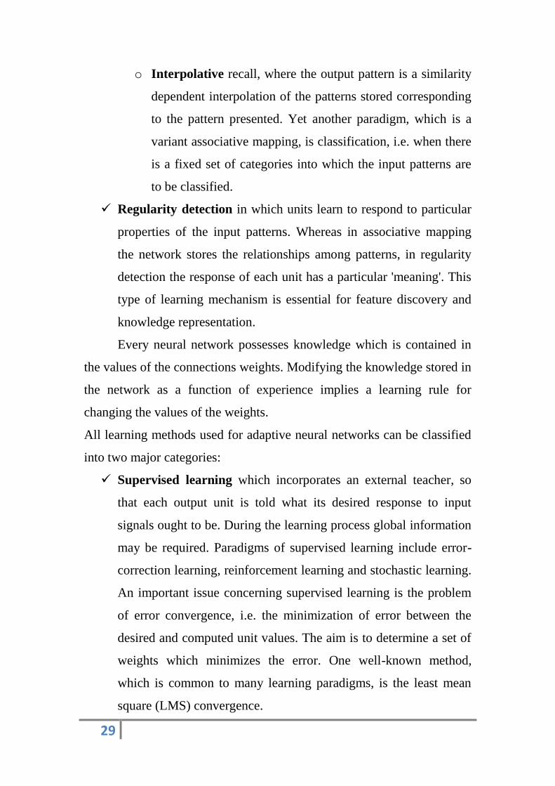
o Interpolative recall, where the output pattern is a similarity

dependent interpolation of the patterns stored corresponding

to the pattern presented. Yet another paradigm, which is a

variant associative mapping, is classification, i.e. when there

is a fixed set of categories into which the input patterns are

to be classified.

Regularity detection in which units learn to respond to particular

properties of the input patterns. Whereas in associative mapping

the network stores the relationships among patterns, in regularity

detection the response of each unit has a particular 'meaning'. This

type of learning mechanism is essential for feature discovery and

knowledge representation.

Every neural network possesses knowledge which is contained in

the values of the connections weights. Modifying the knowledge stored in

the network as a function of experience implies a learning rule for

changing the values of the weights.

All learning methods used for adaptive neural networks can be classified

into two major categories:

Supervised learning which incorporates an external teacher, so

that each output unit is told what its desired response to input

signals ought to be. During the learning process global information

may be required. Paradigms of supervised learning include error-

correction learning, reinforcement learning and stochastic learning.

An important issue concerning supervised learning is the problem

of error convergence, i.e. the minimization of error between the

desired and computed unit values. The aim is to determine a set of

weights which minimizes the error. One well-known method,

which is common to many learning paradigms, is the least mean

square (LMS) convergence.

30

Unsupervised learning uses no external teacher and is based upon

only local information. It is also referred to as self-organization, in

the sense that it self-organizes data presented to the network and

detects their emergent collective properties. Paradigms of

unsupervised learning are Hebbian learning and competitive

learning.A neural network learns on-line if it learns and operates at

the same time. Usually, supervised learning is performed off-line,

whereas unsupervised learning is performed on-line.

Transfer Function [8]:

The behavior of an ANN (Artificial Neural Network) depends on

both the weights and the input-output function (transfer function) that is

specified for the units. This function typically falls into one of three

categories: linear (or ramp), threshold and sigmoid.

For linear units, the output activity is proportional to the total weighted

output. For threshold a unit, the output is set at one of two levels,

depending on whether the total input is greater than or less than some

threshold value. For sigmoid units, the output varies continuously but not

linearly as the input changes. Sigmoid units bear a greater resemblance to

real neurons than do linear or threshold units, but all three must be

considered rough approximations.

2.1.7 Error Calculation [9]:

Error calculation is an important aspect of any neural network.

Whether the neural network is supervised or unsupervised, an error rate

must be calculated. The goal of virtually all training algorithms is to

minimize the error. In this section we will examine how the error is

calculated for a supervised neural network. We will also discuss how the

error is determined for an unsupervised training algorithm. We will begin

this section by discussing two error calculation steps used for supervised

training.

31

Error Calculation and Supervised Training [9]:

Error calculation is an important part of the supervised training

algorithm. In this section we will examine an error calculation method

that can be employed by supervised training. For supervised training

there are two components to the error that must be considered. First, we

must calculate the error for each of the training sets as they are processed.

Secondly we must take the average across each sample for the training

set. For example, the XOR problem that has only four items in its training

set. An output error would be calculated on each element of the training

set. Finally, after all training sets have been processed, the root mean

square (RMS) error is determined.

Output Error:

The output error is simply an error calculation that is done to

determine how far off a neural network's output was from the ideal

network. This value is rarely used for any purpose other than a stepping

stone on the way to the calculation of root mean square (RMS) error.

Once all training sets have been used the RMS error can be calculated.

This error acts as the global error for the entire neural network.

2.1.8 A Feed Forward Neural Network:

A "feed forward" neural network [9] is similar to the types of neural

networks that we are ready examined. Just like many other neural

network types the feed forward neural network begins with an input layer.

This input layer must be connected to a hidden layer. This hidden

layer can then be connected to another hidden layer or directly to the

output layer. There can be any number of hidden layers so long as at least

one hidden layer is provided. In common use most neural networks will

have only one hidden layer. It is very rare for a neural network to have

more than two hidden layers. We will now examine, in detail, and the

structure of a "feed forward neural network".

32

The Structure of a Feed Forward Neural Network:

A "feed forward" neural network differs from the neural networks

previously examined. Figure 2.3 shows a typical feed forward neural

network with a single hidden layer

Figure 2.3. A typical feed forward neural network with a single hidden

layer

Choosing the Network Structure:

As we saw the previous section there are many ways that feed

forward neural networks can be constructed. You must decide how many

neurons will be inside the input and output layers. You must also decide

how many hidden layers you're going to have, as well as how many

neurons will be in each of these hidden layers.

There are many techniques for choosing these parameters. In this

section we will cover some of the general "rules of thumb" that you can

use to assist you in these decisions. Rules of thumb will only take you so

33

far. In nearly all cases some experimentation will be required to

determine the optimal structure for your "feed forward neural network".

The Input Layer:

The input layer to the neural network is the conduit through which

the external environment presents a pattern to the neural network. Once a

pattern is presented to the input later of the neural network the output

layer will produce another pattern. In essence this is all the neural

network does. The input layer should represent the condition for which

we are training the neural network for. Every input neuron should

represent some independent variable that has an influence over the output

of the neural network.

It is important to remember that the inputs to the neural network

are floating point numbers. These values are expressed as the primitive

Java data type "double". This is not to say that you can only process

numeric data with the neural network. If you wish to process a form of

data that is non-numeric you must develop a process that normalizes this

data to a numeric representation.

The Output Layer:

The output layer of the neural network is what actually presents a

pattern to the external environment. Whatever patter is presented by the

output layer can be directly traced back to the input layer. The number of

a output neurons should directly related to the type of work that the

neural network is to perform.

To consider the number of neurons to use in your output layer you

must consider the intended use of the neural network. If the neural

network is to be used to classify items into groups, then it is often

preferable to have one output neurons for each group that the item is to be

assigned into. If the neural network is to perform noise reduction on a

signal then it is likely that the number of input neurons will match the

34

number of output neurons. In this sort of neural network you would one

day he would want the patterns to leave the neural network in the same

format as they entered.

The Number of Hidden Layers:

There are really two decisions that must be made with regards to

the hidden layers. The first is how many hidden layers to actually have in

the neural network. Secondly, you must determine how many neurons

will be in each of these layers. We will first examine how to determine

the number of hidden layers to use with the neural network.

Neural networks with two hidden layers can represent functions

with any kind of shape. There is currently no theoretical reason to use

neural networks with any more than two hidden layers. Further for many

practical problems there's no reason to use any more than one hidden

layer. Problems that require two hidden layers are rarely encountered.

Differences between the numbers of hidden layers are summarized in

Table 2.1.

Number of

Hidden

Layers

Result

None Only capable of representing linear separable

functions or decisions.

1 Can approximate arbitrarily while any

functions which contains a continuous

mapping from one finite space to another.

2 Represent an arbitrary decision boundary to

arbitrary accuracy with rational activation

functions and can approximate any smooth

mapping to any accuracy.

Table 2.1: Determining the number of hidden layers

35

Just deciding the number of hidden neuron layers is only a small

part of the problem. You must also determine how many neurons will be

in each of these hidden layers. This process is covered in the next section.

The Number of Neurons in the Hidden Layers:

Deciding the number of hidden neurons in layers is a very

important part of deciding your overall neural network architecture.

Though these layers do not directly interact with the external environment

these layers have a tremendous influence on the final output. Both the

number of hidden layers and number of neurons in each of these hidden

layers must be considered.

Using too few neurons in the hidden layers will result in something

called under fitting. Under fitting occurs when there are too few neurons

in the hidden layers to adequately detect the signals in a complicated data

set. Using too many neurons in the hidden layers can result in several

problems. First too many neurons in the hidden layers may result in over

fitting. Over fitting occurs when the neural network has so much

information processing capacity that the limited amount of information

contained in the training set is not enough to train all of the neurons in the

hidden layers [9].

A second problem can occur even when there is sufficient training

data. An inordinately large number of neurons in the hidden layers can

increase the time it takes to train the network. The amount of training

time can increase enough so that it is impossible to adequately train the

neural network. Obviously some compromise must be reached between

too many and too few look neurons in the hidden layers.There are many

rule-of-thumb methods for determining the correct number of neurons to

use in the hidden layers.

36

Some of them are summarized as follows.

• The number of hidden neurons should be in the range between the size

of the input layer and the size of the output layer.

• The number of hidden neurons should be 2/3 of the input layer size,

plus the size of the output layer.

• The number of hidden neurons should be less than twice the input

layer size.

These three rules are only starting points that you may want to

consider. Ultimately the selection of the architecture of your neural

network will come down to trial and error. But what exactly is meant by

trial and error. You do not want to start throwing random layers and

numbers of neurons at your network. To do so would be very time-

consuming. There are two methods they can be used to organize your trial

and error search for the optimum network architecture.

There are two trial and error approaches that you may use in

determining the number of hidden neurons are the "forward" and

"backward" selection methods. The first method, the "forward selection

method", begins by selecting a small number of hidden neurons. This

method usually begins with only two hidden neurons. Then the neural

network is trained and tested. The number of hidden neurons is then

increased and the process is repeated so long as the overall results of the

training and testing improved. The "forward selection method" is

summarized in the figure 2.4.

2.1.9 Applications of NN:

Prediction: learning from past experience

o pick the best stocks in the market

o predict weather

o identify people with cancer risk

37

Classification

o Image processing

o Predict bankruptcy for credit card companies

o Risk assessment

Figure 2.4. Selecting the number of hidden neurons with forward

selection

Recognition

o Pattern recognition: SNOOPE (bomb detector in U.S.

airports)

o Character recognition

o Handwriting: processing checks

38

Data association

Not only identify the characters that were scanned but identify

when the scanner is not working properly

Data Filtering

o e.g. take the noise out of a telephone signal, signal

smoothing

Planning

o Unknown environments

o Sensor data is noisy

o Fairly new approach to planning

Advantages:

Adapt to unknown situations

Robustness: fault tolerance due to network redundancy

Autonomous learning and generalization

Disadvantages

Not exact

Large complexity of the network structure

2.1.10 Problems not suited to a Neural Network:

Programs that are easily written out as a flowchart are an example

of programs that are not well suited to neural networks. If your program

consists of well defined steps, normal programming techniques will

suffice [9].Another criterion to consider is whether the logic of your

program is likely to change. The ability for a neural network to learn is

one of the primary features of the neural network. If the algorithm used to

solve your problem is an unchanging business rule there is no reason to

use a neural network. It might be detrimental to your program if the

neural network attempts to find a better solution, and begins to diverge

from the expected output of the program.

39

Finally, neural networks are often not suitable for problems where

you must know exactly how the solution was derived. A neural network

can become very useful for solving the problem for which the neural

network was trained. But the neural network cannot explain its reasoning.

The neural network knows because it was trained to know. The neural

network cannot explain how it followed a series of steps to derive the

answer.

2.1.11 Problems Suited to a Neural Network:

Although there are many problems that neural networks are not

suited for there are also many problems that a neural network is quite

useful for solving. In addition, neural networks can often solve problems

with fewer lines of code than a traditional programming algorithm. It is

important to understand what these problems are. Neural networks are

particularly useful for solving problems that cannot be expressed as a

series of steps, such as recognizing patterns, classifying into groups,

series prediction and data mining.

2.1.12 Validating Neural Networks:

Once a neural network has been trained it must be evaluated to see

if it is ready for actual use. This final step is important so that it can be

determined if additional training is required. To correctly validate a

neural network, validation data must be set aside that is completely

separate from the training data.

As an example, consider a classification network that must group

elements into three different classification groups. You are provided with

10,000 sample elements. For this sample data the group that each element

should be classified into is known. For such a system you would divide

the sample data into two groups of 5,000 elements. The first group would

form the training set. Once the network was properly trained the second

group of 5,000 elements would be used to validate the neural network.

40

It is very important that a separate group always be maintained for

validation. First training a neural network with a given sample set and

also using this same set to predict the anticipated error of the neural

network a new arbitrary set, will surely lead to bad results. The error

achieved using the training set will almost always be substantially lower

than the error on a new set of sample data. The integrity of the validation

data must always be maintained.

This brings up an important question. What exactly does happen if

the neural network that you have just finished training performs poorly on

the validation set? If this is the case, then you must examine what,

exactly, this means. It could mean that the initial random weights were

not good. Rerunning the training with new initial weights could correct

this. While an improper set of initial random weights could be the cause,

a more likely possibility is that the training data was not properly chosen.

If the validation is performing badly this most likely means that

there was data present in the validation set that was not available in the

training data. The way that this situation should be solved is by trying a

different, more random, way of separating the data into training and

validation sets. If this fails, you must combine the training and validation

sets into one large training set. Then new data must be acquired to serve

as the validation data [9].

For some situations it may be impossible to gather additional data

to use as either training or validation data. If this is the case then you are

left with no other choice but to combine all or part of the validation set

with the training set. While this approach will forgo the security of a good

validation, if additional data cannot be acquired this may be your only

alternative.

41

2.2 Introduction to Associative memories:

The associative memory models[10], an early class of neural

models that fit perfectly well with the vision of cognition emergent

from today brain neuro-imaging techniques, are inspired on the

capacity of human cognition to build calculus makes them a possible

link between connectionist models and classical artificial intelligence

developments.

Our memories function as an associative or content - addressable.

That is, a memory does not exist in some isolated fashion, located in a

particular set of neurons. Thus memories are stored in association with

one another. These different sensory units lie in completely separate

parts of the brain, so it is clear that the memory of the person must

be distributed throughout the brain in some fashion. We access the

memory by its contents not by where it is stored in the neural

pathways of the brain. This is very powerful; given even a poor

photograph of that person we are quite good at reconstructing the persons

face quite accurately. This is very different from a traditional

computer where specific facts are located in specific places in

computer memory. If only partial information is available about this

location, the fact or memory cannot be recalled at all.

Traditional measures of associative memory performance are

its memory capacity and content-addressability. Memory capacity

refers to the maximum number of associated pattern pairs that can be

stored and correctly retrieved while content-addressability is the ability

of the network to retrieve the correct stored pattern. Obviously, the

two performance measures are related to each other. It is known that

using Hebb's learning rule in building the connection weight matrix

of an associative memory yields a significantly low memory

capacity. Due to the limitation brought about by using Hebb's

42

learning rule, several Modifications and variations are proposed to

maximize the memory capacity [11].

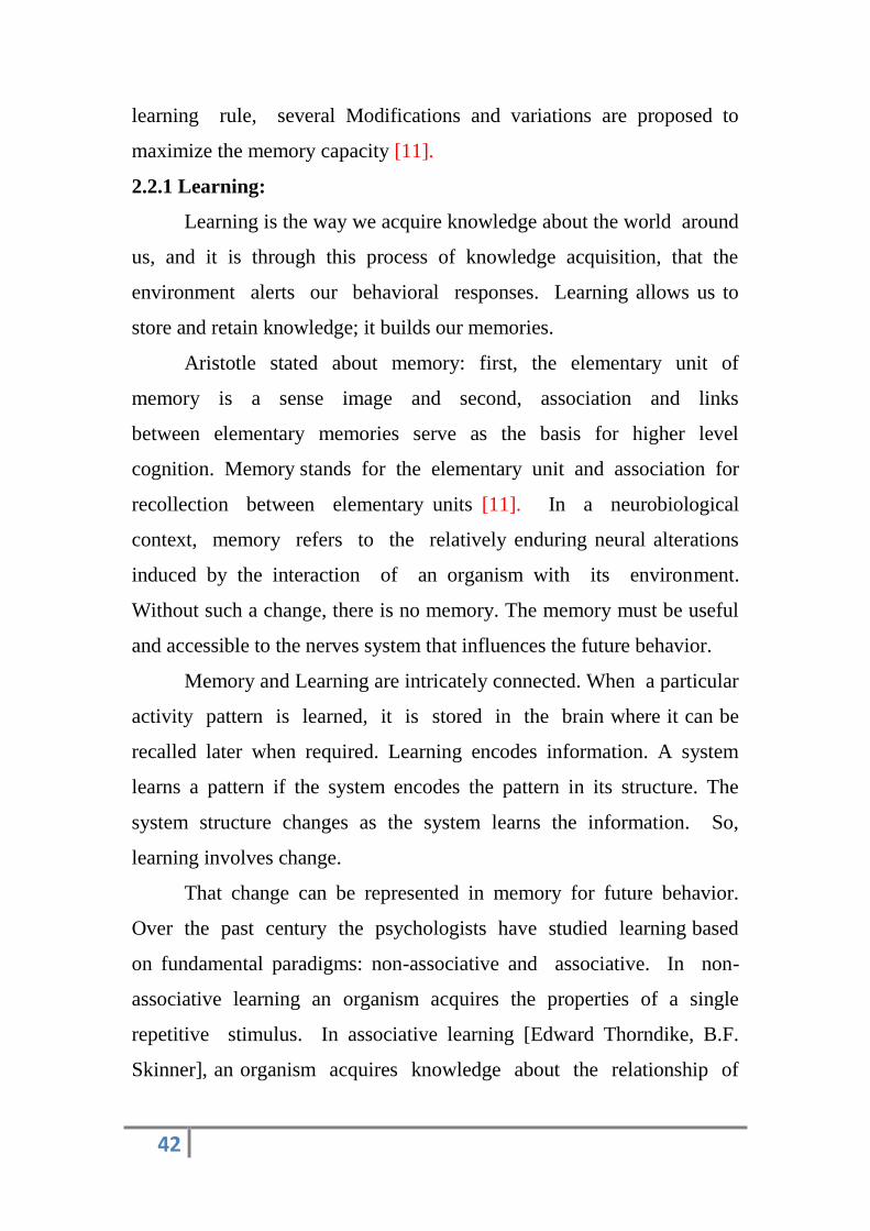
2.2.1 Learning:

Learning is the way we acquire knowledge about the world around

us, and it is through this process of knowledge acquisition, that the

environment alerts our behavioral responses. Learning allows us to

store and retain knowledge; it builds our memories.

Aristotle stated about memory: first, the elementary unit of

memory is a sense image and second, association and links

between elementary memories serve as the basis for higher level

cognition. Memory stands for the elementary unit and association for

recollection between elementary units [11]. In a neurobiological

context, memory refers to the relatively enduring neural alterations

induced by the interaction of an organism with its environment.

Without such a change, there is no memory. The memory must be useful

and accessible to the nerves system that influences the future behavior.

Memory and Learning are intricately connected. When a particular

activity pattern is learned, it is stored in the brain where it can be

recalled later when required. Learning encodes information. A system

learns a pattern if the system encodes the pattern in its structure. The

system structure changes as the system learns the information. So,

learning involves change.

That change can be represented in memory for future behavior.

Over the past century the psychologists have studied learning based

on fundamental paradigms: non-associative and associative. In non-

associative learning an organism acquires the properties of a single

repetitive stimulus. In associative learning [Edward Thorndike, B.F.

Skinner], an organism acquires knowledge about the relationship of

43

either one stimulus to another, or one stimulus to the organisms

own Behavioral response to that stimulus.

On the neuronal basis of formation of memories into two

distinct categories: STM (short term memory) and LTM (long term

memory). Inputs to the brain are processed into STM‘s which last

at the most for a few minutes. Information is downloaded into LTM‘s

for more permanent storage. One of the most important functions of

our brain is the laying down and recall of memories. It is difficult to

imagine how we could function without both short and long term

memory. The absence of short term memory would render most

tasks extremely difficult if not impossible - life would be punctuated by

a series of one time images with no logical connection between

them. Equally, the absence of any means of long term memory would

ensure that we could not learn by past experience.

The acquisition of knowledge is an active, ongoing cognitive

process based on our perceptions. An important point about the learning

mechanism is that it distributes the memory over different areas, making

them robust to damage. Distributed storage permits the brain to work

easily from partially corrupted information [11]. .

2.2.2 Associative Memory Model:

Associative memory maps [10, 12] data from an input space to data

in an output space. In general, this mapping is from unknown

domain points to known range points, where the memory learns an

underlying association from a training data set. For non-learning

memory models, which have their origin in additive neuronal

dynamics, connection strength‘s are ―programmed‖ a priori

depending upon the association that are to be encoded in the system.

Sometimes these memories are referred to as matrix associative

memories, because a connection matrix W, encodes associations

44

where is one of the programmed memories

then is called the association of . When are in

different spaces then the model is hetero- associative memory. i.e. it

associates two different vectors with one another. If , then the

model is Auto-associative memory. i.e., it associates a vector with itself.

Associative memory models enjoy properties such as fault tolerance.

Types of Associative Neural Memories:

Associative neural memories are concerned with associative

learning and retrieval of information (vector patterns) in neural

networks. These networks represent one of the most extensively

analyzed classes of artificial neural networks. Several associative

neural memory models have been proposed over the last two decades.

These memory models can be classified into various ways depending on

Architecture (Static versus Dynamic)

Retrieval Mode (Synchronous versus Asynchronous)

Nature of stored association (Auto-associative versus Hetero-

associative)

Complexity and capability of memory storage

Simple Associative memories are static and very low memory so that

they cannot be applied in the applications where high memory is required

[11]. Several modes can also be used to update the states of the

units in both layers namely synchronous, asynchronous, and a

combination of the two. In synchronous updating scheme, the states

of the units in a layer are updated as a group prior to propagating the

output to the other layer. In asynchronous updating, units in both

layers are updated in some order and output is propagated to the

other layer after each unit update. Lastly, in synchronous-

asynchronous updating, there can be subgroups of units in each

45

layer that are updated synchronously while units in each subgroup are

updated asynchronously.

Dynamic Associative memories such as Hopfield, Bi Directional

Associative memory (BAM), Brain in State Box(BSB) are Dynamical

memories but they also capable of supporting very low memory, so they

cannot be applied in the applications where high memory is required,

because of this reason we chosen Context Sensitive auto-associative

memory model for developing the expert system and also this can be

compared with some of machine learning algorithms such as Back

propagation, Bayesian Networks, C4.5 and Particle Swarm Optimization.

Dynamic Associative memories such as Hopfield, BSB, and

BAM are Dynamical memories but they are also capable of supporting

very low memory, so they cannot be applied in the applications where

high memory requirements are there.

A simple model describing context-dependent associative

memories generates a good vectorial representation of basic logical

calculus. One of the powers of this vectorial representation is the

very natural way in which binary matrix operators are capable to

compute ambiguous situations. This fact presents a biological

interest because of the very natural way in which the human mind is

able to take decisions in the presence of uncertainties. Also these

memories could be used to develop expert agents to the recent problem

domain. Holographic memories are being used to build the many

advanced memory based agents like memory cards, USB Drives,

etc., [11]. The advantage of using recurrent networks as associative

memory is their convergence to one of a finite number of stable states

when started at some initial state. The basic goals are:

• To be able to store as many exemplars as we need, each

corresponding to a different stable state of the network,

46

• To have no other stable state

• To have the stable state that the network converges to be the one

closest

• to the applied pattern

The problems that we are faced with Associative memories:

• The capacity of the network is restricted,

• Depending on the number and properties of the patterns to be

stored,

• some of the exemplar may not be the stable states,

• Some spurious stable states different than the exemplars may arise

by themselves

• The converged stable state may be other than the one closest to the

applied pattern

2.3. Related work:

Not surprisingly, researchers have also tried to use neural networks

in Cryptography. A recent survey of the literature indicates that there has

been an increasing interest in the application of different classes of neural

networks to problems related to cryptography in the past few years.

Recent works have examined the use of neural networks in

cryptosystems. Typical examples include key management, generation

and exchange protocols; visual cryptography; pseudo random generators;

digital watermarking; and steganalysis [13].

2.3.1 Interacting neural network and cryptography:

The goal of any cryptographic system is the exchange of

information among the intended users without any leakage of information

to others who may have unauthorized access to it. A common secret key

could be created over a public channel accessible to any opponent. Neural

networks can be used to generate common secret key.

47

In case of neural cryptography, both the communicating

networks receive an identical input vector, generate an output bit and

are trained based on the output bit. The two networks and their weight

vectors exhibit a novel phenomenon, where the networks synchronize to a

state with identical time-dependent weights. The generated secret key

over a public channel is used for encrypting and decrypting the

information being sent on the channel [14]

Based on chaotic neural networks, a Hash function can be

constructed, which makes use of neural networks' diffusion property

and chaos' confusion property. This function encodes the plaintext of

arbitrary length into the hash value of fixed length (typically, 128-bit,

256-bit or 512-bit). Theoretical analysis and experimental results show

that this hash function is one-way, with high key sensitivity and

plaintext sensitivity, and secure against birthday attacks or meet-in-the-

middle attacks. These properties make it a suitable choice for data

signature or authentication [15].

Neural cryptography deals with the problem of key exchange using

the mutual learning concept between two neural networks. The two

networks will exchange their outputs (in bits) so that the key between the

two communicating parties is eventually represented in the final learned

weights and the two networks are said to be synchronized. Security of

neural synchronization depends on the probability that an attacker can

synchronize with any of the two parties during the training process, so

decreasing this probability improves the reliability of exchanging their

output bits through a public channel [16].Artificial neural networks are

used to classify functional blocks from a disassembled program as being

either cryptography related or not. The resulting system, referred to as

NNLC (Neural Net for Locating Cryptography) [17].

48

When training a neural network it is tempting to experiment with

architectures until a low total error is achieved. The danger in doing so is

the creation of a network that loses generality by over-learning the

training data; lower total error does not necessarily translate into a low

total error in validation. The resulting network may keenly detect the

samples used to train it, without being able to detect subtle variations in

new data. A method is presented for choosing the best neural network

architecture for a given data set based on observation of its accuracy,

precision, and mean square error [18].

The method, based on, relies on k-fold cross validation to evaluate

each network architecture k times to improve the reliability of the choice

of the optimal architecture. The need for four separate divisions of the

data set is demonstrated (testing, training, and validation, as normal, and

a comparison set). Instead of measuring simply the total error the

resulting discrete measures of accuracy, precision, false positive, and

false negative are used. This method is then applied to the problem of

locating cryptographic algorithms in compiled object code for two

different CPU architectures to demonstrate the suitability of the method.

2.4 Passwords:

Basics of Passwords: Passwords are at present the most common method

for verifying the identity of a user. This is a flawed method; systems

continue to use passwords because of their ease of use and ease of

implementation. Among many problems are the successful guessing of

user‘s passwords, and the intercepting of them or uncovering them online.

To prevent guessing and for additional security, the National Security

Agency (NSA) recommends using a random 8-letter password that is

regularly changed [19].

Since such a stream of passwords is almost impossible to

remember (certainly for me), the hapless user is forced to write these

49

passwords down, adding to the insecurity. Thus passwords need to be

protected by cryptographic techniques, whether they are stored or

transmitted. Several simple techniques can help make the old-fashioned

form of passwords easier to memorize. First, the system can present a

user with a list of possible random passwords from which to choose. With

such a choice, there may be one password that is easier for a given user to

remember. Second, the most common passwords are limited to 8

characters, and experience has shown that users have a hard time picking

such a short password that turns out to be secure.

If the system allows passwords of arbitrary length (fairly common

now), then users can employ pass phrases: a phrase or sentence that is not

going to be in dictionaries yet is easy for the given user to remember. My

favorite pass phrase is ―Dexter‘s mother‘s bread,‖ but I won‘t be able to

use it any more. Personal physical characteristics form the basis for a

number of identification methods now in use. The characteristics or

biometrics range from fingerprints to iris patterns, from voice to hand

geometry, among many examples. These techniques are outside the scope

of this book. The remaining two sections study two uses of one-way

functions to help secure passwords. A simple system password scheme

would just have a secret file holding each user‘s account name and the

corresponding password. There are several problems with this method: if

someone manages to read this file, they can immediately pretend to be

any of the users listed. Also, someone might find out about a user‘s likely

passwords from passwords used in the past.

For the reasons above and others, early UNIX systems protected

passwords with a one-way function (described in an earlier chapter).

Along with the account name, the one-way function applied to the

password is stored. Thus given a user A, with account name NA and

password PA, and given a fixed one-way function h, the system would

50

store NA and h (PA) as a table entry in the password file, with similar

entries for other users. When A supplies her password to the system, the

software computes h of her password and compares this result with the

table entry. In this way the systems administrators themselves will not

know the passwords of users and will not be able to impersonate a user.

In early UNIX systems it was a matter of pride to make the

password file world readable. A user would try to guess other‘s

passwords by trying a guess P: first calculate h (P) and then compare this

with all table entries. There were many values of P to try, such as entries

in a dictionary, common names, special entries that are often used as

passwords, all short passwords, and all the above possibilities with

special characters at the beginning or the end. These ―cracker‖ programs

have matured to the point where they can always find at least some

passwords if there are quite a few users in the system. Now the password

file is no longer public, but someone with root privileges can still get to it,

and it sometimes leaks out in other ways.

To make the attack in the previous paragraph harder (that attack is

essentially the same as cipher text searching), systems can first choose h

the one-way function to be more execution time intensive. This only

slows down the searches by a linear factor. Another approach uses an

additional random table entry, called a salt. Suppose for example that

each password table entry has another random t-bit field (the salt),

different for each password. When Alice first puts her password into the

system (or changes it), she supplies PA. The system chooses the salt and

calculates EA = h (PA, SA), where h is fixed up to handle two inputs

instead of one.

The password file entry for Alice now contains A, SA, and EA.

With this change, an attack on a single user is the same, but the attack of

the previous paragraph on all users at the same time now takes either an

51

extra factor of time equal to either 2t or the number of users, whichever is

smaller. Without the salt, an attacker could check if ―Dexter‖ were the

password of any user by calculating h (“Dexter”) and doing a fast search

of the password file for this entry. With the salt, to check if Alice is using

―Dexter‖ for example, the attacker must retrieve Alice‘s salt SA and

calculate h (“Dexter”, SA). Each user requires a different calculation, so

this simple device greatly slows down the dictionary attack.

Text Password:

Password strength is a measure of the effectiveness of

a password in resisting guessing and brute-force attacks. In its usual form,

it estimates how many trials an attacker who does not have direct access

to the password would need, on average, to guess it correctly. The

strength of a password is a function of length, complexity, and

unpredictability [20]

However, other attacks on passwords can succeed without a brute

search of every possible password. For instance, knowledge about a user

may suggest possible passwords (such as pet names, children's names,

etc.). Hence estimates of password strength must also take into account

resistance to other attacks as well. Using strong passwords lowers

overall risk of a security breach, but strong passwords do not replace the

need for other effective security controls. The effectiveness of a password

of a given strength is strongly determined by the design and

implementation of the authentication system software, particularly how

frequently password guesses can be tested by an attacker and how

securely information on user passwords is stored and transmitted. Risks

are also posed by several means of breaching computer security which

are unrelated to password strength.

52

Determining Password Strength:

There are two factors to consider in determining password strength:

the ease with which an attacker can check the validity of a guessed

password, and the average number of guesses the attacker must make to

find the correct password. The first factor determined by how the

password is stored and what it is used for, while the second factor is

determined by how long the password is, what set of symbols it is drawn

from and how it is created.

Password Guess Validation:

The most obvious way to test a guessed password is to attempt to

use it to access the resource the password was meant to protect. However,

this can be slow and many systems will delay or block access to an

account after several wrong passwords are entered. On the other hand,

systems that use passwords for authentication must store them in some

form to check against entered values. Usually only a cryptographic of a

password is stored instead of the password itself. If the hash is strong

enough, it is very hard to reverse it, so an attacker that gets hold of the

hash value cannot directly recover the password. However, if the

cryptographic hash data files have been stolen, knowledge of the hash

value lets the attacker quickly test guesses.

Password Creation:

Passwords are created either automatically (using randomizing

equipment) or by a human. The strength of randomly chosen passwords

against a brute force attack can be calculated with precision. Commonly,

passwords are initially created by asking a human to choose a password,

sometimes guided by suggestions or restricted by a set of rules. This

typically happens at the time of account creation for computer systems or

Internet Web sites. In this case, only estimates of strength are possible,

53

since humans tend to follow patterns in such tasks, and those patterns

may assist an attacker [21].

Password strength depends on symbol set and length:

Increasing the number of possible symbols from which random

passwords are chosen will increase the strength of generated passwords of

any given length. For example, the printable characters in the American

Standard Code for Information Interchange (ASCII) character set

(roughly those on a standard U.S. English keyboard) include 26 letters (in

two case variants), 10 digits, and 33 non-alphanumeric symbols (i.e.,

punctuation, grouping, etc.), for a total of 94 symbols (95 if space is

included). However the same strength can always be achieved with a

smaller symbol set by choosing a longer password. In the extreme, binary

passwords can be very secure, even though they only use two possible

symbols. Thus a 14 character password consisting of only random

lowercase letters has the same strength (4.7×14 = 65.8 bits) as a ten

character password chosen at random from all printable ASCII characters

(65.55 bits).

Guide Lines for Passwords:

Common guidelines for choosing good passwords are designed to

make passwords less easily discovered by intelligent guessing [16-19]:

Password length should be around 12 to 14 characters if permitted,

and longer still if possible while remaining memorable

Use randomly generated passwords where feasible

Avoid any password based on repetition, dictionary words, letter or

number sequences, usernames, relative or pet names, romantic

links (current or past), or biographical information (e.g., ID

numbers, ancestors names or dates).

Include numbers, and symbols in passwords if allowed by the

system

54

If the system recognizes case as significant, use capital and lower-

case letters

Avoid using the same password for multiple sites or purposes

If you write your passwords down, keep the list in a safe place,

such as a wallet or safe, not attached to a monitor or in an unlocked

desk drawer

Protecting passwords:

Computer users are generally advised to "never write down a

password anywhere, no matter what" and "never use the same password

for more than one account." However, an ordinary computer user may

have dozens of password-protected accounts. Users with multiple

accounts needing passwords often give up and use the same password for

every account. When varied password complexity requirements prevent

use of the same (memorable) scheme for producing high-strength

passwords, overly simplified passwords will often be created to satisfy

irritating and conflicting password requirements. A Microsoft expert was

quoted as saying at a 2005 security conference: "I claim that password

policy should say you should write down your password. I have 68

different passwords. If I am not allowed to write any of them down, guess

what I am going to do? I am going to use the same password on every one

of them [20].

Limitations of alphanumeric passwords:

The main problem with the alphanumeric passwords is that once a

password has been chosen and learned the user must be able to recall

it to log in. But, people regularly forget their passwords. If a password

is not frequently used it will be even more susceptible to forgetting.

The recent surveys have shown that users select short, simple

passwords that are easily guessable, for example, personal names of

their family members, names of pets, date of birth etc [25].the most

55

important issue is having a password that can be remembered reliably

and input quickly. They are unlikely to give priority to security over their

need to get on with their work.

Graphical Passwords:

Graphical password were originally described by

Blonder(1996).the basic need for graphical password is that graphical

passwords are expected to be easier to recall, less likely to be

written down and have the potential to provide a richer symbol

space than text based password. For example, a user might authenticate

by clicking a series of points on an image, selecting a series of tiles, or by

drawing lines on the screen [26]. Because human beings live and interact

in an environment where the sense of sight is predominant for most

activities, our brains are capable of processing and storing large amounts

of graphical information with ease. While we may find it very hard to

remember a string of fifty characters, we are able easily to remember

faces of people, places we visited, and things we have seen. These

graphical data represent millions of bytes of information and thus provide

large password spaces. Thus, graphical password schemes provide a way

of making more human-friendly passwords while increasing the level of

security.

Disadvantages of Graphical Passwords:

Dictionary attacks are infeasible, partly because of the large

password space, but mainly because there are no pre-existing searchable

dictionaries for graphical information. It is also difficult to devise

automated attacks. Whereas we can recognize a person's face in less than

a second, computers spend a considerable amount of time processing

millions of bytes of information regardless of whether the image is a face,

a landscape, or a meaningless shape.

56

Graphical password schemes have been proposed as a possible

alternative to text-based schemes, motivated partially by the fact that

humans can remember pictures better than text; psychological studies

supports such assumption [27]. Pictures are generally easier to be

remembered or recognized than text. In addition, if the number of

possible pictures is sufficiently large, the possible password space of a

graphical password scheme may exceed that of text- based schemes and

thus presumably offer better resistance to dictionary attacks. Because of

these (presumed) advantages, there is a growing interest in graphical

password. In addition to workstation and web log-in applications,

graphical passwords have also been applied to ATM machines and

mobile devices. A comprehensive survey of the existing graphical

password techniques has been conducted. We will discuss the strengths

and limitations of each method and also point out future research

directions in this area. In conducting this survey, we want to answer the

following questions: are graphical passwords as secure as text

passwords?, what is the major design and implementation issues for

graphical passwords?

2.5. Traditional Password Authentication:

In current web-based login protocols, a person logs in to a service

provider by sending his user identity and password to the server in

question, who then looks up the corresponding record in its database, and

performs a comparison to determine whether the password is valid. The

password is typically not stored in plaintext, but rather, a ―salted one-way

function‖ of the password is stored. This means that if somebody gains

access to the database of the service provider, they will not be able to

obtain plaintext passwords. However, the password itself is generally sent

prior to have the salted one-way function applied. In order to protect the

session against an eavesdropper, it is common to encrypt the transmission

57

of the password. However, passwords are only used in situations where

the two communicating machines do not store any prior cryptographic

key – if they did, then passwords would be an inferior alternative to

standard cryptographic authentication mechanisms such as digital

signatures (such as RSA) or message authentication codes (such as Hash-

based Message Authentication Code (HMAC)).

2.5.1 Vulnerabilities of current password authentication practices:

There are many potential attacks that can be mounted on the

common password authentication method. To begin with, one should

notice that the above described method does not offer any protection

against an attack in which an attacker claims to be a service provider, and

convinces a user to attempt to log in – clearly, if there is no encryption,

then the attacker will simply obtain the password of his victim. The same

holds if encryption is used, but the attacker sends his a public key to

which it knows the corresponding secret key to the user instead of that of

the bank‘s. This may occur even if certificates are employed [28]; In fact,

in many, if not most, scenarios, average users are not capable of

distinguishing authentic from illegitimate certificates.

Recently, this type of attack has become a very common, and is

used by attackers wanting to perform identity theft, also referred to as

phishing. Its popularity can be seen by noting with the now daily

examples of so-called phishers trying to harvest passwords by sending out

emails that appear to originate from a bank. Even though the phishers‘

success rate is relatively low, this is a profitable attack, as evidenced by

how common it is. This is due to the ease with which attackers can spam

large populations at a negligible cost, and the straightforwardness of

spoofing emails. There are indications that the problem may become

worse as attacker become more sophisticated [30].

58

2.5.2 Password Authenticated Protocols:

User authentication could be defined as a process in which one

party is assured of the identity of a second party involved in the protocol.

It is generally accomplished by one or more of the following [30]:

a) Something known. Examples include standard passwords, Personal

Identification Numbers (PINs), and the secret or private keys

whose knowledge is used in challenge-response protocols.

b) Something possessed. This is normally a physical accessory like,

magnetic striped cards, chip cards and hand-held customized

calculators (password generators) which provide time-variant

passwords.

c) Something inherent (to a human individual). This category includes

methods which make use of physical characteristics and actions of

human beings(biometrics), such as handwritten signatures,

fingerprints, voice, retinal patterns, hand geometries, and dynamic

keyboarding characteristics.

The least expensive and the most convenient solutions for user

authentication have been based on the first category. But authentication

without key exchange would not help much. These two topics need to be

considered jointly rather than separately. As pointed out in [31], a

protocol providing authentication without 33key exchange is susceptible

to an enemy who would wait until the authentication is complete and then

takes over one end of the communications line. Same is the case with key

exchange that is independent of authentication. So it is quite important to

make sure that the key exchanged is in fact shared with the intended party

and not an adversary.

In [32], the authors of Symbol Native Application Programming

Interface (SNAPI) classify user authentication schemes into those that

require persistent data to be stored on the user‘s system and those that do

59

not. The former category includes schemes similar to Secure Shell (SSH),

where persistent participant specific information is stored on the client‘s

system. As mentioned above these schemes require extra security

assumptions. The second category includes password based protocols like

the popular (Encrypted key exchange) EKE family protocols. These were

later followed by Augmented-EKE (A-EKE), Modified-EKE (M-EKE),

Simple Password EKE (SPEKE), Diffe-Hellman EKE (DH-EKE), Secure

Remote Password protocol (SRP) and so on.

In recent years several password-only protocols have been proposed and

the reason for growing importance is they are based on direct trust

between a user and a server, and do not require the user to store long

secrets or data on the user‘s system. These protocols can be used not only

for user authentication with the server but also for mutual authentication

between any two users. Below we summarize the characteristics of

password-based key establishment protocols:

1. The passwords selected by users usually belong to a small dictionary

and have small entropy which makes it possible for the adversary to

search through all possible passwords in a reasonable time.

2. On-line dictionary attacks should not be possible. This means that

the adversary should not be able to partition the dictionary into valid

and invalid passwords by just gathering information during a valid

exchange.

3. On-line dictionary attacks should not be feasible. These attacks can

be easily detected, and thwarted, by counting access failures.

4. Should provide for mutual authentication.

2.5.3 Attacks against Passwords:

Many systems break because they rely on user-generated

passwords. Left to themselves, people don't choose strong passwords. If

they're forced to use strong passwords, they can't remember them. If the

60

password becomes a key, it's usually much easier and faster to guess the

password than it is to brute-force the key; we've seen elaborate security

systems fail in this way. Some user interfaces make the problem even

worse: limiting the passwords to eight characters, converting everything

to lower case, etc. Even passphrases can be weak: searching through 40-

character phrases is often much easier than searching through 64-bit

random keys. We've also seen key-recovery systems that circumvent

strong session keys by using weak passwords for key-recovery.

2.5.4 Alternatives to Password Authentication:

The numerous ways in which permanent or semi-permanent

passwords can be compromised has prompted the development of other

techniques. Unfortunately, some are inadequate in practice, and in any

case few have become universally available for users seeking a more

secure alternative.

Single-use passwords are only valid once makes many potential attacks

ineffective. Most users find single use passwords extremely inconvenient.

They have, however, been widely implemented in personal online

banking, where they are known as Transaction Authentication

Numbers (TANs). As most home users only perform a small number of

transactions each week, the single use issue has not led to intolerable

customer dissatisfaction in this case.

Time-synchronized one-time passwords are similar in some ways to

single-use passwords, but the value to be entered is displayed on a small

(generally pocketable) item and changes every minute or so.

Pass Window one-time passwords are used as single-use passwords, but

the dynamic characters to be entered are visible only when a user

superimposes a unique printed visual key over a server generated

challenge image shown on the user's screen.

61

Access controls based on public key cryptography e.g. SSH. The

necessary keys are usually too large to memorize and must be stored on a

local computer, security token or portable memory device, such as a USB

flash drive or even floppy disk.

Biometric methods promise authentication based on unalterable personal

characteristics, but currently (2008) have high error rates and require

additional hardware to scan, for example, fingerprints, irises, etc. They

have proven easy to spoof in some famous incidents testing commercially

available systems, for example, the gummie fingerprint spoof

demonstration,[33] and, because these characteristics are unalterable, they

cannot be changed if compromised; this is a highly important

consideration in access control as a compromised access token is

necessarily insecure.

Single sign-on technology is claimed to eliminate the need for having

multiple passwords. Such schemes do not relieve user and administrators

from choosing reasonable single passwords, nor system designers or

administrators from ensuring that private access control information

passed among systems enabling single sign-on is secure against attack.

As yet, no satisfactory standard has been developed.

Evaluating technology is a password-free way to secure data on e.g.

removable storage devices such as USB flash drives. Instead of user

passwords, access control is based on the user's access to a network

resource.

Non-text-based passwords, such as graphical passwords or mouse-

movement based passwords.[34] Graphical passwords are an alternative

means of authentication for log-in intended to be used in place of

conventional password; they use images, graphics or colors instead

of letters, digits or special characters. One system requires users to select

a series of faces as a password, utilizing the human brain's ability to recall

62

faces easily.[35] In some implementations the user is required to pick

from a series of images in the correct sequence in order to gain

access.[36] Another graphical password solution creates a one-time

password using a randomly-generated grid of images. Each time the user

is required to authenticate, they look for the images that fit their pre-

chosen categories and enter the randomly-generated alphanumeric

character that appears in the image to form the one-time password. [37,

38] .So far, graphical passwords are promising, but are not widely used.

Studies on this subject have been made to determine its usability in the

real world. While some believe that graphical passwords would be harder

to crack, others suggest that people will be just as likely to pick common

images or sequences as they are to pick common passwords.

2D Key (Two-Dimensional Key) is a 2D matrix-like key input method

having the key styles of multiline passphrase, crossword, ASCII/Unicode

art, with optional textual semantic noises, to create big password/key

beyond 128 bits to realize the MePKC (Memorizable Public-Key

Cryptography) using fully memorizable private key upon the current

private key management technologies like encrypted private key, split

private key, and roaming private key.

Cognitive passwords use question and answer cue/response pairs to verify

identity.

2.5.5 Traditional authentication schemes and their disadvantages:

Normally system assigns usernames and passwords to each and every

authorized user. In order to check whether a user is authorized or not each

server stores all these usernames and passwords in a table. Whenever a

user wants to get a service from the server he uses his username and

password ,then server uses information stored in the password table to

check whether the user is authorized or not.

63

USER NAME PASSWORD

Harsh 25-may1991

Vamsi Vss123

Suresh Abecke

Aditya Letmein

Sanjay 24dk03k

Table 2.2. Password table

In order to enhance the security of the system proposed work certain

encryption algorithms on the passwords and the password in the password

table will be in the encrypted format.

USER NAME ENCRYPTED PASSWORD

Harsha ↑ǨNʒ╚⌡

Vamsi kJɊ 26v

Suresh D₧£ȣ

Aditya ¥~Ϳ� ¥2p

Sanjay efeaeolg

Table 2.3. Verification table

There are many limitations in using this type of approach. Attacker

can easily change the details of users by using attacks like SQL-Injection

and the password table occupies lot of memory in the server.

2.6 Probabilistic Approach Feed Forward Neural Network:

In feed forward network the output of neurons (unit) in one layer

will be passed as input to the next layer and this process continues until

the output layer units gets an input from previous layers. Finally these

output units yield an output. The output of network depends on Input,

64

Connection strengths (Weight values), and Output function used in each

layer. If we modify any of the above the output of the network will be

changed. By taking this fact as an advantage we can perform encryption

so that no attacker can decrypt it easily.

Here if „P‟ is a row matrix representing input and „W‟ is a matrix

representing weights of the network then a feed forward network

produces cipher text in the following way.

(2.1)

Plain Text Cipher Text

Figure 2.5. Feed forward Network

2.6.1 Weight Matrix Calculation:

In order to generate unique Cipher text for given plain text we have to

designate weight matrix whose RANK is equal to length of the plain text.

So here Determinant of (DET) Weight matrix should not be Zero.

i.e. |Weight Matrix

|≠0 (2.2)

65

A Weight Matrix

, ( 2.3)

The weight matrix can be defined in C# as follows:

Matrix weightMatrix = new Matrix (3,2);

The threshold variable is not multidimensional, like the weight matrix.

There is one threshold value per neuron. Each neuron in the second layer

has an individual threshold value. These values can be stored in an array

of C# double variables. The following code shows how the entire

memory of the two layers can be defined.

Matrix weightMatrix = new Matrix (3,2);

double [] thresholds = new double[2];

These declarations include both the 3x2 matrix and the two threshold

values for the second layer. There is no need to store threshold values for

the first layer, since it is not connected to another layer. Weight matrix

and threshold values are only stored for the connections between two

layers, not for each layer. The preferred method for storing these values

is to combine the thresholds with the weights in a combined matrix. The

above matrix has three rows and two columns. The thresholds can be

thought of as the fourth row of the weight matrix, which can be defined

as follows:

Matrix weightMatrix = new Matrix(4,2);

The combined threshold and weight matrix is described in equation

2.4. In this equation, the variable w represents the cells used to store

weights and the variable t represents the cells used to hold thresholds.

66

A Threshold and Weight Matrix

, (2.4)

Combining the thresholds and weights in one matrix has several

advantages. This matrix now represents the entire memory of this layer of

the neural network and you only have to deal with a single structure.

This work gives the facility of defining own character set and normalize

the character set.

2.6.2Defining Own Character Set:

In order to define a character set this work defines characters in the

character set in a particular order and Maximum or Minimum value of the

character set. Any organization which wants to use this technique can

define their own character set. If the organization wants to use existing

character sets like ASCII, UNICODE etc., they can use them and in

order. To enhance the security they can change the order of characters

and value assigned to each character.

Character Unique

code

Character Unique

code

Character Unique

code

A 11 J 20 S 29

B 12 K 21 T 30

C 13 L 22 U 31

D 14 M 23 V 32

E 15 N 24 W 33

F 16 O 25 X 34

G 17 P 26 Y 35

H 18 Q 27 Z 36

I 19 R 28

Table 2.4. Example Character Set

67

The table 2.4 shows a character set with the minimum value is 11 and

maximum value is 36 for the characters. This technique assigns any user

defined minimum and maximum values for the set.

2.6.3 Normalizing Character Set:

In normalization we will convert each unique number assigned to a

character in to probabilistic value.

Here we use following formula to find probabilistic value of each

character.

�� �

� ����������������������

Where Cn is the normalized value of the taken character, Cmax is the

maximum value of the character set; Cmin is the minimum value of the

character set and Ct the value of taken character. Here in this method we

get Cn values in the range [0, 1].

Character Probabilistic

value

Character Probabilistic

value

Character Probabilistic

value

A 0.00 J 0.36 S 0.72

B 0.04 K 0.40 T 0.76

C 0.08 L 0.44 U 0.80

D 0.12 M 0.48 V 0.84

E 0.16 N 0.52 W 0.88

F 0.20 O 0.56 X 0.92

G 0.24 P 0.60 Y 0.96

H 0.28 Q 0.64 Z 1.00

I 0.32 R 0.68

Table 2.5. Normalized Character Set

68

Changing order of characters

This method uses existing standard character sets and can

improve security by changing order of charters and , minimum value to

change unique number and probabilistic values associated to each

character so that attacker may confuse in guessing the unique numbers or

probabilistic values. For example by changing order of characters

listed in table 2.5, the following changes can be observed in table 2.6.

Character Unique

code

Character Unique

code

Character Unique

code

A 11 J 20 S 29

Z 12 G 21 Q 30

C 13 F 22 U 31

M 14 D 23 E 32

V 15 N 24 W 33

L 16 I 25 H 34

K 17 P 26 Y 35

X 18 T 27 B 36

O 19 R 28

Table 2.6. Changes in Unique code after changing the order of

characters

Character Probabilistic

value

Character Probabilistic

value

Character Probabilistic

value

A 0.00 J 0.36 S 0.72

Z 0.04 G 0.40 Q 0.76

C 0.08 F 0.44 U 0.80

M 0.12 D 0.48 E 0.84

V 0.16 N 0.52 W 0.88

L 0.20 I 0.56 H 0.92

K 0.24 P 0.60 Y 0.96

X 0.28 T 0.64 B 1.00

O 0.32 R 0.68

Table 2.7. Changes in probabilistic values after changing the order of

characters

69

If we observe in table 2.6, the change in the order of the alphabets,

make the unique code assigned to them changed automatically and after

normalization the probabilistic values also changed. This provides more

secure authentication if this input is given for password authentication

schemes.

Advantages of the Proposed Method:

Since this method provides opportunity to change the character set

and the unique code for character, this method is very difficult to attack

thus provides more security. In order to decrypt the cipher text, attacker

has to identify the weight matrix .Though he identifies the weight matrix

he may not know the algorithm used ,number of hidden layers, output

function used, character set (Including order of characters in character

set), minimum and maximum values used in character set. Even one

element of matrix changes attacker cannot decrypt the cipertext. The

security this method can be enhanced by increasing number of hidden

layers in the network. The users of this algorithm can define their own

character set, by doing so users can add new characters into their

character set.

Disadvantages:

There is a chance of noise when we give the input and any noise in

cipher text will make the decryption very tough. In order to decrypt the

cipher text there is a need to calculate inverse of the weight matrix.

2.6.4 Implementation Details:

Once the password is given, and the‖Encrypt‖ button is pressed, a

corresponding probablistic value and corresponding weight matrix can be

identified and obseved.. This applicationcan provide probalblistic values

for different passwords .If the weight matrix is changed the encrypted

password also changes and it provides the users of this application to take

different weight matrices while encrypting the password,

70

Figure 2.6. Password Encryption in to Probabilistic Values

Here if the weight matrix is changed the changes in the encrypted

text, can be visualized and observed in the figure 2.7.

Figure 2.7. Probabilistic values after Weight Matrix Change

71

2.7 Proposed Work:

As it is already discussed, the proposed method uses a neural network

approach to the authentication using a feed forward neural network and

the input to the network is the usernames and the output will be the

passwords. When a particular user submits his login credentials, his

username is given as input to network and we check whether the output

of network and specified password are equal or not, if both are equal the

user is authorized and rejected otherwise. In this work a separate

character set for alphanumeric data including special characters is design

using the ASCII, GRAY CODE, EBCDIC and UNICODE characters.

The next step is to normalization. Normalize each character in to

probabilistic values in the range [0, 1]. The Normalized password data is

supplied as input to a multi associative memory neural network with one

or more hidden layers. This produces encoded password in real values

within the range [0, 1]. We can get decoded data in to character notation

(for memorization and backup) after applying de normalization function.

Guessing password data is given as input for any on associative memory

algorithm with one or more hidden layers to produce decrypted data. If it

is matched the password is authenticated, otherwise it is invalid. After

performing the training, all the weight values are stored in a weight table.

Whenever a user submits his login credentials, network uses this weight

values to produce the output. In order to define a character set, the

following things are used. i. change the order of the characters in a

particular character set and ii. set the Maximum and Minimum values for

the character set.

Any organization which wants to use this novel password

authentication technique can define their own character set by changing

the order of the characters in the character set and giving their own

maximum and minimum values for the Character Set. If the organization

72

wants to use existing character sets like ASCII, UNICODE etc., still they

can use our technique and in order to increase security they can change

the order of characters and even the weights can also be changed by them.

Here the back propagation algorithm, the Hopfield method, the concepts

of the bidirectional associative memory and the brain state in box for both

alphanumeric and graphical password scheme, have been used by which

the level of security is enhanced.