– 12S-1– SUPPLEMENT TO CHAPTER 12 FLOWSHEET CONTROLLABILITY ANALYSIS 12S.0 OBJECTIVES This chapter supplement introduces quantitative measures for controllability assessment to be used when developing the base-case design and in the detailed design stage (Stages 2 and 3, Table 12.1) and highlights how their integration into the design process can help to generate improved flowsheets that satisfy control performance criteria. At this point, the process creation stage has been completed and several promising process flowsheets exist. As they are evaluated, the control objectives are considered as constraints, the latter including: • Adequate disturbance resiliency, that is, the ability to reject disturbances quickly enough to meet specifications • Insensitivity to model uncertainty, that is, the ability to control easily, and to provide adequate closed-loop performance, with relatively insensitivity to model inaccuracies. An approach is introduced to screen the potential designs as early as possible, to identify the most promising designs for rigorous testing in stage 4, in which plantwide controllability assessment is completed. As demonstrated in this chapter supplement, it is important to verify the approximate analysis using rigorous dynamic simulation. Detailed multimedia instruction on the use of ASPEN HYSYS for dynamic simulation is available as part of the multimedia support that may be downloaded from the Wiley web site associated with this book. UNISIM and CHEMCAD could be used also for dynamic simulation. It is assumed that the reader is familiar with the basic concepts of linear systems theory. This material is covered typically in an introductory course on process dynamics and control at the undergraduate level. The subjects in that course that are prerequisite to understanding the concepts in this chapter supplement are: 1. Basic linear matrix theory, linearization, complex numbers, and Laplace and Fourier transforms. Note that Section 12S.1 provides some of this background material.

Chapter 12
Dec 13, 2015
Process controllability and resiliency analysis.
Welcome message from author
This document is posted to help you gain knowledge. Please leave a comment to let me know what you think about it! Share it to your friends and learn new things together.
Transcript

– 12S-1–
SUPPLEMENT TO CHAPTER 12 FLOWSHEET CONTROLLABILITY ANALYSIS
12S.0 OBJECTIVES
This chapter supplement introduces quantitative measures for controllability assessment to
be used when developing the base-case design and in the detailed design stage (Stages 2 and 3,
Table 12.1) and highlights how their integration into the design process can help to generate
improved flowsheets that satisfy control performance criteria. At this point, the process creation
stage has been completed and several promising process flowsheets exist. As they are evaluated,
the control objectives are considered as constraints, the latter including:
• Adequate disturbance resiliency, that is, the ability to reject disturbances quickly enough to
meet specifications
• Insensitivity to model uncertainty, that is, the ability to control easily, and to provide
adequate closed-loop performance, with relatively insensitivity to model inaccuracies.
An approach is introduced to screen the potential designs as early as possible, to identify
the most promising designs for rigorous testing in stage 4, in which plantwide controllability
assessment is completed. As demonstrated in this chapter supplement, it is important to verify the
approximate analysis using rigorous dynamic simulation. Detailed multimedia instruction on the
use of ASPEN HYSYS for dynamic simulation is available as part of the multimedia support that
may be downloaded from the Wiley web site associated with this book. UNISIM and CHEMCAD
could be used also for dynamic simulation.
It is assumed that the reader is familiar with the basic concepts of linear systems theory.
This material is covered typically in an introductory course on process dynamics and control at the
undergraduate level. The subjects in that course that are prerequisite to understanding the concepts
in this chapter supplement are:
1. Basic linear matrix theory, linearization, complex numbers, and Laplace and Fourier
transforms. Note that Section 12S.1 provides some of this background material.

– 12S-2–
2. Pole and zero positions in the complex plane, and their impact on the time-domain
response of linear systems.
3. Linear stability theory and the impact of feedback.
4. Tuning of single-input, single-output controllers (P, PI, and PID controllers). Note that
Section 12S.4 provides instruction on model-based PI-controller tuning.
Key concepts relating to linear process models are reviewed in the first section of the
chapter. For deeper coverage, the reader is referred to the following undergraduate-level texts:
Bequette, B.W., Process Dynamics: Modeling, Analysis, and Simulation, Prentice Hall, Englewood
Cliffs, NJ, (2003).
Luyben, W.L., Process Modeling, Simulation and Control for Chemical Engineers, 2nd ed.,
McGraw-Hill, New York (1990).
Ogunnaike, B.A., and W.H. Ray, Process Dynamics, Modeling and Control, Oxford Univ. Press,
New York (1994).
Seborg, D.E., T.F. Edgar, and D.A. Mellichamp, Process Dynamics and Control, Wiley, New York
(1989).
Stephanopoulos, G., Chemical Process Control, Prentice-Hall, Englewood Cliffs, NJ (1984).
This supplement to Chapter 12,
1. Explains how to generate linear process models in their standard forms.
2. Defines quantitative measures that are used to analyze the controllability and resiliency
(C&R) of process flowsheets, and shows how to implement them using MATLAB.
3. Describes a method to carry out C&R analysis using the results of steady-state process
simulations.
4. Shows how to use quantitative analysis with steady-state and dynamic relative gain
arrays (RGA and DRGA) to reliably select control loop pairings and to use the IMC
model-based approach to provide preliminary tuning of single-loop PI controllers.
5. Analyzes, in Section 12S.5, selected case studies in Chapter 12 to demonstrate the
utility of the quantitative methods. For completeness, these analyses are verified with
dynamic simulations using single-loop PI controllers.
– 12S-3–
After reading this chapter, the student should
1. Be able to compute the frequency-dependent process transfer functions P , dP using
MATLAB, given a linear model in one of its standard forms.
2. Generate the C&R measures: relative-gain array (RGA), and disturbance cost (DC),
given the matrices P s and dP s, describing the effects of the manipulated
variables and disturbances on the process outputs, using MATLAB.
3. Select the appropriate pairings for a decentralized control system for a process using the
static and dynamic RGAs and appropriate resiliency measures, and provide preliminary
tuning using IMC-PI tuning rules.
4. Perform C&R analysis to select between alternative process configurations, given the
results of process simulations using linearized models.
12S.1 GENERATION OF LINEAR MODELS IN STANDARD FORMS
In this chapter supplement, several methods are described to assist the designer in rejecting
designs that do not provide acceptable closed-loop performance, using models linearized about a
steady state. These are generated by expressing the open-loop response of the process outputs, ys,
in terms of the variations of the inputs, us, and disturbances, ds:
sdsPsusPsy d+= (12S.1)
The procedure for deriving the linear state-space model and the input-output transfer
function model in Eq. (12S.1) involves the following steps:
Step 1. The nonlinear state and output equations are derived from the material and energy balances
that model the process. These are expressed in the form:
duxgy
duxfdt
xd
,,
,,
=
= (12S. 2)
– 12S-4–
where x is a vector of nx state variables, y is a vector of ny output (measured) variables,
u is a vector of nu manipulated variables, d is a vector of nd disturbances, and f and g
are vectors of nx and ny nonlinear functions, respectively.
Step 2. The state and output equations are solved at a stationary (steady) state that is defined either
in terms of the desired state variable values or those of the input variables:
***
***d,u,xgy
d,u,xf=
= 0 (12S.3)
where the stationary point is at *** dduu,xx === and . The solution of Eq. (12S.3)
requires that the degrees of freedom of the process be resolved through the specification of
nu+ nd values.
Step 3. The equations are linearized in the vicinity of the desired stationary point, by a Taylor
series expansion of Eq. (12S. 2):
( ) ( ) ( ) ( ) ( ) ( )
* * * * * *
* * * * * *
, , h.o.t.
, , h.o.t.U D
U D
d x f x u d A x x B u u B d ddty g x u d C x x D u u D d d
≅ + − + − + − +
≅ + − + − + − + (12S.4)
Note that the linear approximation is obtained by ignoring the higher order terms (h.o.t.)
of the Taylor series expansion. The matrices UDU D,C,B,B,A and DD are the Jacobian
matrices of appropriate dimension evaluated at the stationary point, defined as follows:
*** d,u,xj
ij,i x
faA∂∂
≡= *** d,u,xj
ij,i x
gcC∂∂
≡=
*** d,u,xj
ij,i,UU u
fbB∂∂
≡= *** d,u,xj
ij,i,UU u
gdD∂∂
≡=
*** d,u,xj
ij,i,DD d
fbB∂∂
≡= *** d,u,xj
ij,i,DD d
gdD∂∂
≡=
Step 4. The linearized equations are formulated in terms of perturbation variables that express the
deviation from the stationary point (or steady state): *xxx −= , *yyy −= , *uuu −= and

– 12S-5–
*ddd −= . Substituting the perturbation variables into Eqs. (12S.4) and ignoring higher-
order terms:
dDuDxCy
dBuBxAdt
xd
DU
DU
++≅
++≅ (12S.5)
Eqs. (12S.5) constitute the linear state-space representation of the system.
Step 5. The linearized equations are transformed into the Laplace domain:
sdsPsusPsy d+= , (12S.1)
where ( ) UU DBAIsCsP +−⋅= −1 and ( ) DDd DBAIsCsP +−⋅= −1 are matrices of the
appropriate dimension. Eq. (12S.1) constitutes the input-output transfer function
representation of the linear system.
As an example, the procedure for generating linear models in standard form is demonstrated
for an exothermic reactor, whose complete analysis is presented in Case Study 12S.1 of Section
12S.5.
Example 12S.1 Standard Linear Models for an Exothermic Reactor.
A continuous-stirred-tank reactor for the production of propylene glycol is analyzed in Case Study
12S.1, in Section 12S.5 below. Approximate linear models for the reactor are generated using the
five-step procedure as follows:
Step 1. Define the State and Output Equations. The hydrolysis of propylene oxide (PO) to
propylene glycol is an exothermic reaction catalyzed by H2SO4:
CH2-O-CH-CH3 + H2O → CH2OH-CH-OH-CH3
When water is supplied in excess, the reaction is second order with respect to the propylene oxide
concentration and zero order with respect to the water concentration. Its rate constant exhibits an
Arrhenius dependence on temperature, with k0 = 3.294×1026 m3/(kmol-h) and E = 1.556×10⁵
kJ/kmol. Furthermore, it is customary to dilute the PO feed with methanol (MeOH), while the
H2SO4 catalyst enters the reactor with the feed. Operating conditions are sought for carrying out

– 12S-6–
this liquid-phase reaction in a 47-ft3 continuous-stirred-tank reactor (CSTR), with the liquid holdup
at 85% of its total volume (1.135 m3). The liquid feeds are fed at 23.9 oC, with one consisting of
18.712 kmol/h of PO and 32.73 kmol/h of MeOH. The water feed rate is from 160 – 500 kmol/h
(2.84 – 8.88 m3/h), selected to moderate the reactor temperature. To reduce the risk of vaporization,
the reactor is operated at a pressure of 3 bar. Under these conditions, the transients for the PO
concentration, CPO [kmol/m3], and temperature, T [oC], are determined by solving the following
species and enthalpy balances:
( ) 20PO
wPOin,POPO CTkV
qqCVdt
dC−
+−
ℑ= (12S.6)
( ) ( )( )V
TTqqHCTkCdt
dT wPO
P
0021 −+−∆−= (12S.7)
where, ( )2273.TR/EoekTk +−= m3/(kmol-h), R = 8.314 kJ/kmol-K, the molar flow rate of PO in
the feed, ℑPO,in = 18.712 kmol/h, V = 1.135 m3, ∆H = –9×10⁴ kJ/kmol, the organic volumetric feed
rate, q0= 2.556 m3/h, the water volumetric feed rate is qw, T0 = 23.9 oC, and cP = 3,558 kJ/ m3 oC.
Implicit in the assumption of perfect level control is the pairing between the effluent volumetric
flow rate, F, and the liquid level, L. This leaves the temperature, T, as the output, to be controlled
by the water feed rate, qw, as the manipulated variable. The disturbances to the process are the
volumetric organic feed rate, q0, and the feed temperature, T0. Thus, [ ]TPO T,Cx = , [ ]Ty = ,
[ ]wqu = and [ ]Toin,PO T,d ℑ= .
Step 2. Solve at the Steady State. The state equations are solved at the steady state. The degrees of
freedom are resolved by fixing all of the input variable values and solving the two equations for the
two unknown state variables.
( ) 020 =−+
−ℑ
POwPOin,PO CTk
VqqC
V
(12S.8)
( ) ( )( ) 01 002 =−+
−∆−V
TTqqHCTkC
wPO
P
(12S.9)
Taking *u = qw* = 5.325 m3/h and [ ] [ ]TTo*in,PO* .,.T,d 923 71218=ℑ= and solving Eqs. (12S.8)
and (12S.9) gives [ ]T* ,.x 2.48 060= . Note that the fractional conversion of PO is X = 1 –

– 12S-7–
CPO/CPO,in = 1 – 0.06/2.374 = 0.975, where CPO,in = ℑPO,in/(q0 + qw). This solution is obtained
analytically, graphically (see Case Study 12S.1), or using a numerical method (e.g., the Newton-
Raphson method).
Steps 3 and 4. Linearize in the Vicinity of the Steady State. The Jacobian matrices for the linearized
approximation are:
( )
( ) ( ) ( )
∆−∂
∂+
+−
∆−∂
∂−−
+−
=
P
*PO**w*PO*
P
*PO*
*PO**w
CCH
TTk
VqqCTk
CH
CTTkCTk
Vqq
A 20
20
2
2
601 (12S.10)
( )
−−
−=
VTT
VC
B**
*PO
U 0601 , ( )
+=
Vqq
VB*wD 00
01
601 (12S.11)
[ ]10=C , [ ]0=UD , [ ]00=DD (12S.12)
The division by 60 in each matrix is to express time in minutes instead of hours. Note also that all
of the variables are expressed in physical units. Substituting numerical values into Eqs. (12S.10)
and (12S.11):
−−=
887008229039602039
....
A ,
−−
=8596000090..
BU ,
=
115700001470
..
BD
These matrices are scaled by assuming that all outputs and manipulated variables are nominally at
50% of their ranges, and the disturbance variable values are constrained to vary in the range ∆d =
[±50% ±5 oC]T. Thus:
=
−−== −
*
*POxxxs T
CS,
....
SASA0
08870016440
435520391
*wuuUxs,U qS,..
SBSB =
−−
== −
05550078201
ℑ=
== −
50050
007000033021 *in,PO
ddDxs,D.
S,.
.SBSB
(12S.13)
– 12S-8–
These matrices relate the input (manipulated and disturbance) variables to the output (controlled)
variables, with all of the variables scaled and in perturbation variable form.
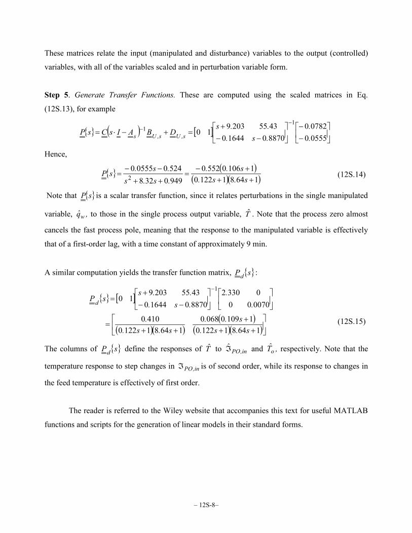
Step 5. Generate Transfer Functions. These are computed using the scaled matrices in Eq.
(12S.13), for example
( ) [ ]
−−
−−
+=+−⋅=
−−
0555007820
887001644043552039
101
1
.
..s...s
DBAIsCsP s,Us,Us
Hence,
( )( )( )164811220
1106055209490328524005550
2 +++−
=++
−−=
s.s.s..
.s.s.s.sP (12S.14)
Note that sP is a scalar transfer function, since it relates perturbations in the single manipulated
variable, wq , to those in the single process output variable, T . Note that the process zero almost
cancels the fast process pole, meaning that the response to the manipulated variable is effectively
that of a first-order lag, with a time constant of approximately 9 min.
A similar computation yields the transfer function matrix, sPd :
[ ]
( )( )( )
( )( )
++
+++
=
−−
+=
−
164811220110900680
1648112204100
00700003302
887001644043552039
101
s.s.s..
s.s..
..
.s...s
sPd
(12S.15)
The columns of sPd define the responses of T to in,POℑ and oT , respectively. Note that the
temperature response to step changes in in,POℑ is of second order, while its response to changes in
the feed temperature is effectively of first order.
The reader is referred to the Wiley website that accompanies this text for useful MATLAB
functions and scripts for the generation of linear models in their standard forms.
– 12S-9–
21.2 QUANTITATIVE MEASURES FOR CONTROLLABILITY AND RESILIENCY
The quantitative assessment of the controllability and resiliency of chemical processes has
generated considerable interest. The term resiliency was introduced by Morari (1983), who also
pioneered qualitative measures for its assessment. Furthermore, Perkins (1989) presented an
approach for the simultaneous design of processes and their control systems that addresses
plantwide controllability directly.
All of the C&R measures use the linear approximations, sP and sPd , which describe
the effects of the control variables and disturbances, respectively, on the process outputs. A
commonly used controllability measure is the relative-gain array (RGA – Bristol, 1966), which
relies only on sP . The disturbance condition number (DCN; Skogestad and Morari, 1987) and
the disturbance cost (DC; Lewin, 1996) are resiliency measures that require a disturbance model,
sPd , in addition to sP . These C&R measures are especially useful in Stages 2 and 3 of the
design process (see Table 12.1) because they do not assume a controller structure or a specific
controller design and tuning.
It is assumed that each input variable is nominally at the midpoint of its range and is
expressed in perturbation variable form, and scaled by dividing by its nominal value. For example,
if Fi is an inlet flow rate, nominally at 500 lbmol/hr, its operating range is 0 ≤ Fi ≤ 1000 lbmol/h, in
perturbation variable form, −500 ≤ Fi ≤ 500, and in scaled form, −1 ≤ Fi ≤ 1. Thus, sP and
sPd are scaled by multiplying the gains in each column by the nominal value of the appropriate
input variable. As a result, all of the scaled inputs vary over the same range [−1, 1]. Note, however,
that the RGA is scale independent, whereas the DC is input scale dependent.

– 12S-10–
Relative-gain Array (RGA)
Steady-State RGA (Bristol, 1966)
Figure 12S.1 shows the block diagram for a multiple-input, multiple-output (MIMO)
process to be controlled by two single-loop controllers. Having closed one of the loops (y1 − u1), the
controller in the second loop, which manipulates u2 based on the feedback of y2, must be tuned. A
desirable feature of this controller is to have the effective process gain remain invariant, regardless
of the action of the other control loop.
c1 p11
p21
p12
p22
u1y1
y2u2
-
Figure 12S.1 MIMO process with one control loop.
When the controller c1 is put into manual operation, i.e., when it is turned off, the process
gain as seen by controller c2 is
yu
pc
2
222
1 ,OL= (12S.16)
where u2 and y2 are the deviations of the input and output from their nominal values in the steady
state. On the other hand, when c1 is put into automatic operation, the process gain as seen by
controller c2 is
yu
p p cp c
pc
2
222 12
1
11 121
11,CL
= −+
(12S.17)
In general, for MIMO systems, a useful measure is the ratio
process gain as seen by a given controller with all other loops open process gain as seen by a given controller with all other loops closed

– 12S-11–
When this ratio is close to unity, the given controller is relatively insensitive to interaction.
Computing this ratio for the MIMO process in Figure 12S.1:
21111
11222
22
2
2
2
2
11
1
pcp
cpp
p
uy
uy
CL,c
OL,c
+−
= (12S.18)
When the top loop is closed-loop stable, and when c1 has integral action,
lim
scp c p→ +
=0 1
11
11 1 11
Therefore, the ratio at steady state is
21122211
2211
21111
11222
22
2
2
2
2
10
lim0
lim
1
1
pppppp
pcp
cpp
ps
uy
uy
s
CL,c
OL,c
−=
+−
→=→ (12S.19)
Similarly,
lims
yu
yu
p pp p p p
c OL
c CL
→=
−−0
2
1
2
1
12 21
11 22 12 21
1
1
,
,
(12S.20)
Thus, for a two-input, two-output process, the RGA is defined as
( )
2 2
2 2
1 1
1 1
1 1
1 2, ,
1 1
1 2, , 111 12 11 22 12 21
21 22 12 21 11 222 2
1 2, ,
2 2
1 2, ,
det
c OL c OL
c CL c CL
c OL c OL
c CL c CL
y yu u
y yu u p p p p
Pp p p py y
u u
y yu u
−
λ λ − Λ = = = ⋅ λ λ −
(12S.21)
In general, the RGA can be computed using
( )TPP 1−⊗=Λ (12S.22)
where ⊗ denotes the element-by-element (Schur) product.
– 12S-12–
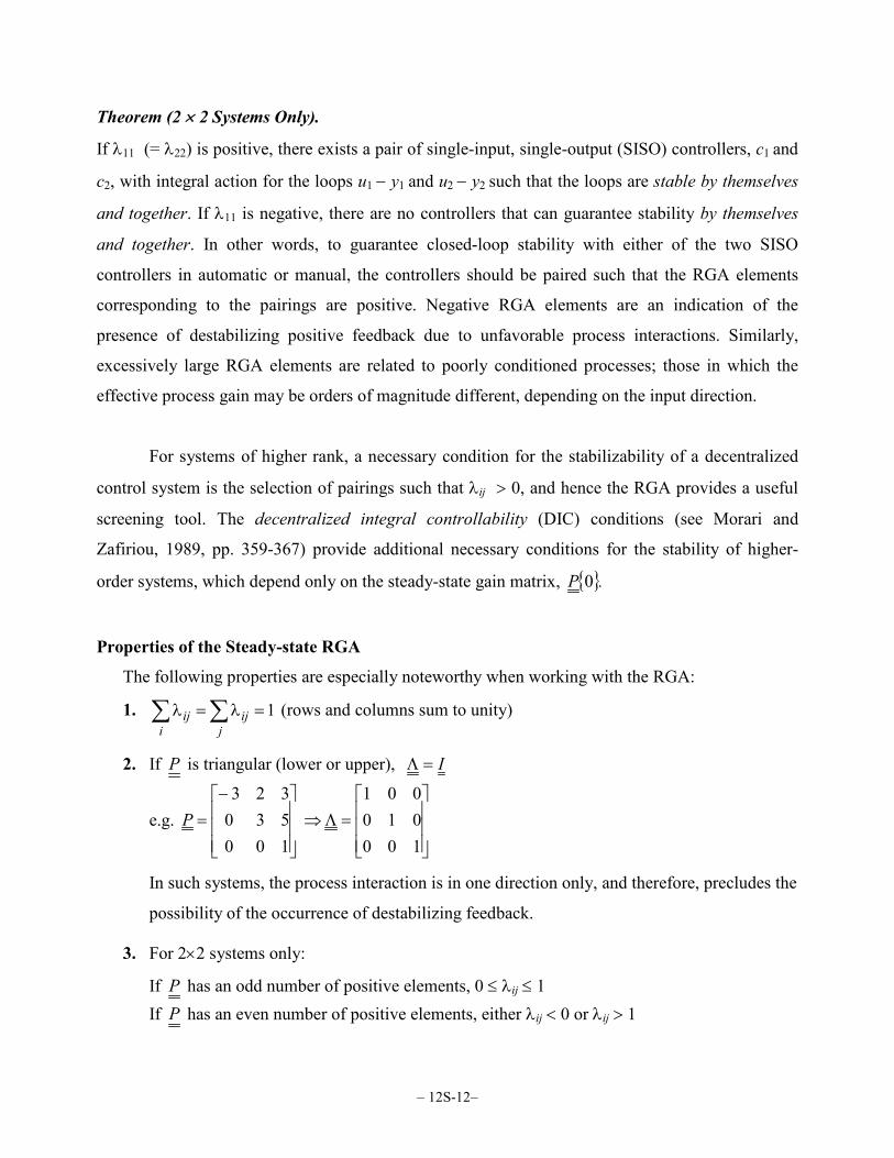
Theorem (2 × 2 Systems Only).
If λ11 (= λ22) is positive, there exists a pair of single-input, single-output (SISO) controllers, c1 and
c2, with integral action for the loops u1 − y1 and u2 − y2 such that the loops are stable by themselves
and together. If λ11 is negative, there are no controllers that can guarantee stability by themselves
and together. In other words, to guarantee closed-loop stability with either of the two SISO
controllers in automatic or manual, the controllers should be paired such that the RGA elements
corresponding to the pairings are positive. Negative RGA elements are an indication of the
presence of destabilizing positive feedback due to unfavorable process interactions. Similarly,
excessively large RGA elements are related to poorly conditioned processes; those in which the
effective process gain may be orders of magnitude different, depending on the input direction.
For systems of higher rank, a necessary condition for the stabilizability of a decentralized
control system is the selection of pairings such that λij > 0, and hence the RGA provides a useful
screening tool. The decentralized integral controllability (DIC) conditions (see Morari and
Zafiriou, 1989, pp. 359-367) provide additional necessary conditions for the stability of higher-
order systems, which depend only on the steady-state gain matrix, .P 0
Properties of the Steady-state RGA
The following properties are especially noteworthy when working with the RGA:
1. 1ij iji jλ = λ =∑ ∑ (rows and columns sum to unity)
2. If P is triangular (lower or upper), I=Λ
e.g.
=Λ⇒
−=
100010001
100530323
P
In such systems, the process interaction is in one direction only, and therefore, precludes the
possibility of the occurrence of destabilizing feedback.
3. For 2×2 systems only:
If P has an odd number of positive elements, 0 ≤ λij ≤ 1 If P has an even number of positive elements, either λij < 0 or λij > 1

– 12S-13–
Dynamic RGA (McAvoy, 1983)
Considering the same MIMO process in Figure 12S.1, y2 is expressed in terms of u1and u2:
2221212 upupy += (12S.23)
When c1 is in manual operation, u1 = 0 and
yu
pc
2
222
1 ,OL=
as for the steady-state analysis. When c1 is in automatic operation and it is assumed that the first
loop can be designed to give perfect control (i.e., the first loop's output is assumed to be held at its
set point),
y p u p u u pp
u1 11 1 12 2 112
1120= + = ⇒ = − (12S.24)
Substituting for u1 in Eq. (12S.23),
yu
p p ppc
2
222
12 21
111 ,CL= − (12S.25)
Hence, the dynamic RGA (DRGA) has precisely the same form as the steady-state array. Note that
the dynamic RGA assumes perfect control, which may not be an appropriate assumption, especially
at high frequencies. The computation of the DRGA requires care since it involves complex algebra.
Because columns and rows sum to unity only at the steady state, the DRGA should be computed
using:
( ) ωλ⋅λ=ω jsignDRGA ijijij 0 , (12S.26)
with λijjω computed conveniently for 2 × 2 systems using Eqs. (12S.19) and (12S.20), or using
Eq.(12S.22) in general.
An accepted rule of thumb is to avoid pairings between variables with negative RGA
elements and to select those with values close to unity, as illustrated in the following example.

– 12S-14–
Example 12S.2 LV Control of a Binary Distillation Column
Figure 12S.2 shows the LV configuration for the two-point composition control of a binary
distillation column discussed in Example 12.9. After assigning manipulated variables to regulate
the vapor and liquid inventories, the boilup rate, V, and the reflux flow rate, L, remain available to
control the distillate and bottoms product compositions, xD and xB, respectively. To assess the
controllability and resiliency of this configuration, the disturbances are taken to be the feed
composition, xF, and the flow rate, F. The column dynamics are approximated by a linear model in
transfer function form (Sandelin et al., 1990):
+
=
−
+−−
+−
−+
−+
−
−+
−+
−
−+
−+
−
Fs
s..s
s..
ss.
.ss.
s.s.s.
s..
s.s
.s.s..
B
D
xF
ee
eeVL
ee
eexx
129650
155160
1580040
1100010
50110
55051118
230
50111
048050118
0450
(12S.27)
To complete the process model definition, it is noted that the process input ranges are as follows: L
= 60 ± 60 kmol/h, V = 72 ± 72 kmol /h, F = Fnom ± 20 kmol /h, xF = xF, nom ± 6 %. In Eq. (12S.27),
the gain coefficients are in the appropriate units, and time is in minutes.
Figure 12S.2 Control of a binary distillation column using the LV configuration.
The qualitative guidelines presented in Chapter 12 are not sufficient to decide how to pair the two
manipulated variables with the two outputs. Without analysis, it is not clear whether this pairing
should be diagonal (i.e., xD−L, xB−V as shown in Figure 12S.2) or off-diagonal (i.e., xD−V,
xB−L ). However, using Eq. (12S.19), λ11 in the RGA is

– 12S-15–
11 2211
11 22 12 211.8p p
p p p pλ = =
− (12S.28)
Using the property that the RGA rows and columns add to unity,
−
−=Λ
8.18.08.08.1
,
and consequently, diagonal pairing is recommended, with the off-diagonal pairing resulting in
stability problems, either when both of the controllers are on automatic or when one of the
controllers is switched to manual operation. Although stable, significant interactions are anticipated
when both loops are closed, because of the large RGA element.
Figure 12S.3 Closed-loop response of the LV
configuration for binary distillation to the worst-
case disturbance, d = [20, 6]T, with decentralized
PI control - Outputs: xD (solid line), xB (dashed
line); Inputs: L (solid line), V (dashed line).
To verify this, Figure 12S.3 shows the closed-loop response for the process, diagonally paired with
IMC-tuned PI controllers (xD − L loop: Kc = -50, τI = 8 min; xB − V loop: Kc = 5, τI = 10 min). For
the IMC-PI tuning rules, the reader is referred to Section 12S.4. The simulation is computed for the
worst-case disturbance, d = [20, 6]T, identified using the disturbance cost analysis, to be discussed
shortly. As expected, the response is stable but shows significant interactions, with the bottoms
composition affected more significantly. The reader can try out this example under MATLAB,
using the interactive C&R Tutorial CRGUI available on the Wiley website that accompanies this
text. In the main menu, opt for the “Binary Column.”
In some cases, the RGA elements vary significantly with the frequency, which may indicate
bandwidth limitations on the diagonal dominance of the process. For this example, Figure 12S.4
– 12S-16–
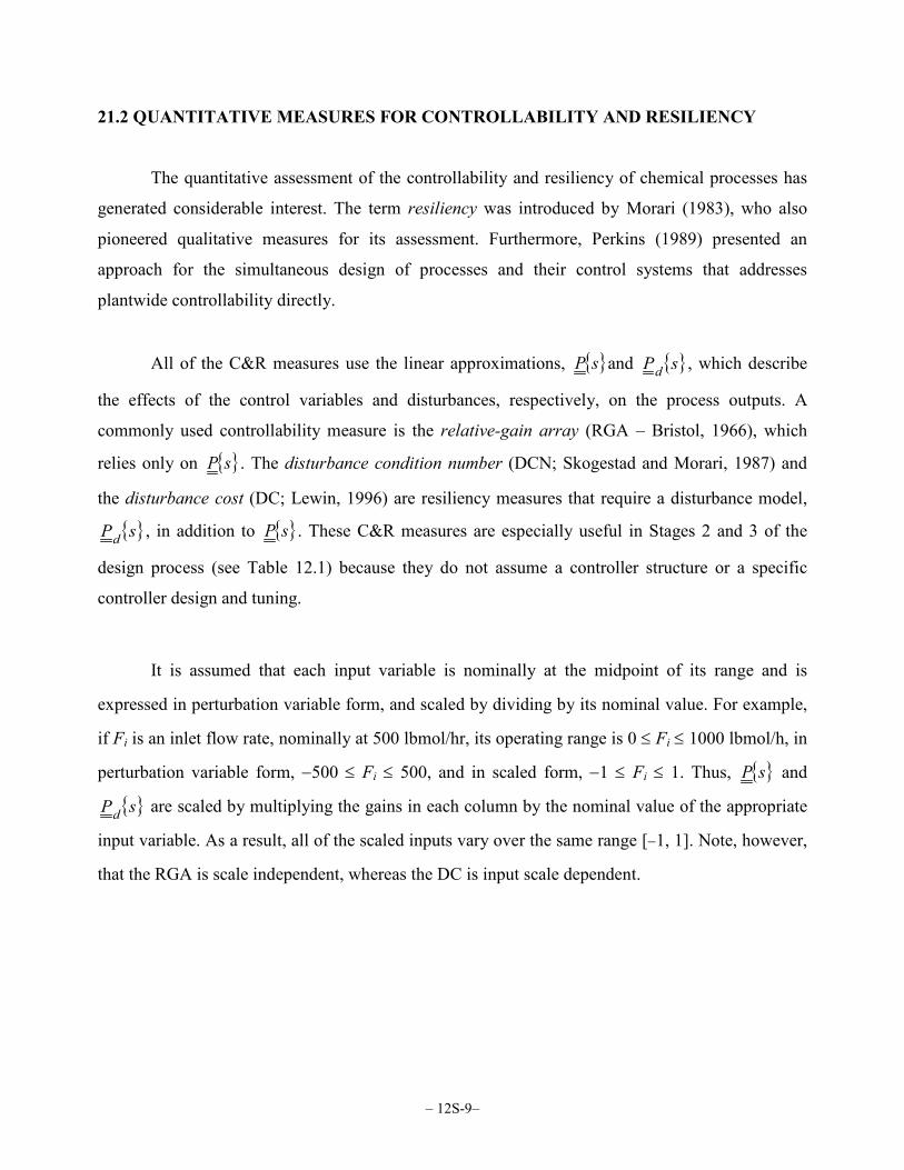
shows λ11 and λ12 as a function of the frequency. Although there is considerable variation at high
frequencies, the diagonal dominance holds for the entire frequency range of interest. In this case,
the RGA and DRGA give the same pairing recommendations. For some processes, however, the
information furnished by the dynamic RGA can be crucial for the correct pairing selection. The
following example provides one such case.
Figure 12S.4 Dynamic RGA for the diagonal
(solid line) and off-diagonal (dotted line) pairings
for Example 12S.2.
Example 12S.3 Importance of the Dynamic RGA
Consider the process:
( )( )
+
=
−
+−−
+−
−+
−+
−
−+
−+
+−
++
2
15
11022
151
5110
32110
4
2
15
1204
131
1455
1211552
2
1
dd
ee
eeuu
e
e
yy
ss
ss
ss
ss
sss
ss
ss.
(12S.29)
Here the process inputs are limited to the ranges: u1 = 60 ± 60, u2 = 50 ± 50, d1 = d 1,nom ± 20, and
d 2 = d 2,nom ± 5, and time is in minutes.
For this system, λ11 = 2/3 in the steady-state RGA, suggesting that the variables be paired
diagonally. In the dynamic RGA, however, the diagonal dominance deteriorates at moderate
frequencies, as shown in Figure 12S.5. In fact, the process is off-diagonally dominant in the
frequency range of interest. The open-loop time constants are on the order of 10 min, and hence,
frequencies in the range 0.1 < ω < 1 rad/min are of particular interest. For this system, the off-
diagonal pairing (i.e., y1 − u2 and y2 − u1) is preferred, contrary to the pairing suggested by the
steady-state RGA. To verify the analysis in Figure 12S.5, the two pairings are simulated using

– 12S-17–
IMC-PI tuning rules (see Section 21.4). For the diagonal pairing, the controllers are tuned: y1 − u1
loop, Kc = 0.6, τI = 15 min; y2 − u2 loop, Kc = −0.37, τI = 20 min. In contrast, for the off-diagonal
pairing, the controller tuning parameters are: y2 − u1 loop, Kc = 10, τI = 3 min; y1 − u2 loop: Kc = 2,
τI = 4 min. Note that the controller gains for the diagonal pairing are an order of magnitude lower
than for the off-diagonal pairing, a reflection of the bandwidth limitations imposed by the delays on
the diagonal elements of the process transfer-function matrix. For a unit-step increase in the y1
setpoint, Figure 12S.6 shows that although the diagonal controller is bandwidth limited, the tuning
for the off-diagonal configuration can be arbitrarily aggressive, only restricted by the actuator
constraints. The reader can try out this example under MATLAB, using the interactive C&R
Tutorial CRGUI available on the Wiley website that accompanies this text. In the main menu, opt
for the “Mystery Process.”
Figure 12S.5 Dynamic RGA for the diagonal
(solid line) and off-diagonal (dotted line) pairings
for Example 12S.3.
Figure 12S.6 Closed-loop response for Example
12S.3 with PI control for a setpoint change in y1
using: (a,b) diagonal pairing; (c,d) off-diagonal
pairing. Shown on the top row are outputs: y1
(solid line), y2 (dashed line), and on the bottom
row, inputs: u1 (solid line), u2 (dashed line).
– 12S-18–
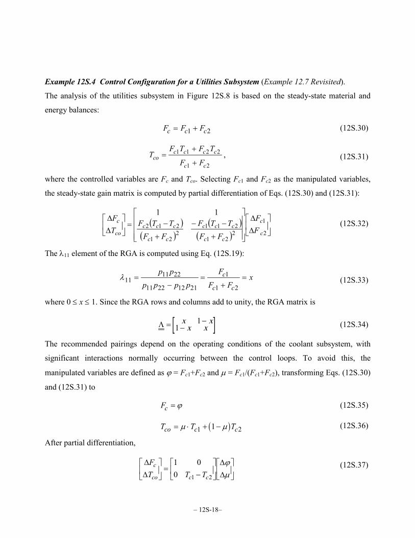
Example 12S.4 Control Configuration for a Utilities Subsystem (Example 12.7 Revisited).
The analysis of the utilities subsystem in Figure 12S.8 is based on the steady-state material and
energy balances:
F F Fc c c= +1 2 (12S.30)
TF T F T
F Fco
c c c c
c c
=+
+1 1 2 2
1 2
, (12S.31)
where the controlled variables are Fc and Tco. Selecting Fc1 and Fc2 as the manipulated variables,
the steady-state gain matrix is computed by partial differentiation of Eqs. (12S.30) and (12S.31):
( )( )
( )( )
∆∆
+
−−
+
−=
∆∆
2
1
221
2112
21
212
11
c
c
cc
ccc
cc
cccco
c
FF
FFTTF
FFTTF
TF
(12S.32)
The λ11 element of the RGA is computed using Eq. (12S.19):
λ1111 22
11 22 12 21
1
1 2=
−=
+=
p p
p p p p
F
F Fxc
c c (12S.33)
where 0 ≤ x ≤ 1. Since the RGA rows and columns add to unity, the RGA matrix is
[ ]Λ = −−x x
x x1
1 (12S.34)
The recommended pairings depend on the operating conditions of the coolant subsystem, with
significant interactions normally occurring between the control loops. To avoid this, the
manipulated variables are defined as ϕ = Fc1+Fc2 and µ = Fc1/(Fc1+Fc2), transforming Eqs. (12S.30)
and (12S.31) to
Fc = ϕ (12S.35)
( )T T Tco c c= ⋅ + −µ µ1 21 (12S.36)
After partial differentiation,
∆∆
−
=
∆∆
µϕ
21001
ccco
c
TTTF
(12S.37)

– 12S-19–
This is a decoupled system that requires diagonal pairings, because I=Λ .
Figure 12S.7 An attractive control configuration for the utilities subsystem.
These pairings, shown in Figure 12S.7, are intuitively correct in that the total flow rate is controlled
by the sum of the two utility streams, and the coolant temperature is controlled by the fraction of
the coolant flowing through the heating system. Note that the temperature and flow controllers
manipulate the variables µ and ϕ, respectively, which are processed by a decoupler, D, to generate
corrections to the two flow rates, Fc1 and Fc2, according to:
( )
−=⋅=
µϕµϕ
1 2
1
c
c
FF
(12S.38)
Example 12S.5 Control Configuration for a Debottlenecked Distillation Column
Often, process design modifications can lead to potential control problems, as demonstrated by
McAvoy (1983) for a distillation column in which the reboiler capacity is doubled by the addition
of an identical reboiler in parallel with the original one (i.e., the column is debottlenecked), as
shown in Figure 12S.8.
Figure 12S.8 Debottlenecked distillation column.
– 12S-20–
A MIMO control system must be configured for the retrofitted column. To compute the RGA, a
linearized model, in the steady state, relates the changes in the designated outputs, T, L1, and L2, to
those of the manipulated variables, Q1, Q2, and B:
∆∆∆
=
∆∆∆
BQQ
aaaaaaaaa
LLT
2
1
333231
232221
131211
2
1 (12S.39)
Since B does not affect T directly, 0=∆∆ BT . Furthermore, by symmetry,
211211 Q
TQTaa
∆∆
=∆∆
== BL
BLaa
∆∆
=∆∆
== 213323
2
2
1
13221 Q
LQLaa
∆∆
=∆∆
== 1
2
2
13122 Q
LQLaa
∆∆
=∆∆
==
Hence, Eq. (12S.39)) becomes
11 11 1
1 21 21 23 2
2 21 21 23
0T a a QL a a a QL a a a B
∆ ∆ ∆ = β ∆ ∆ β ∆
(12S.40)
where
22 1 2
21 1 1
effect of on 1effect of on
a Q La Q L
β = = <
Using Eq. (12S.22),
( )1 0.5 0.51 10.5 0.51 1
0.5 0.5 0
0.5
0.5
TP P− − β
−β −β
− β−β −β
Λ = ⊗ =
(12S.41)
Note that β < 1 and is close to unity. Assuming β = 0.95, the RGA becomes
−−=Λ
501059505910
05050
..
....
(12S.42)
To ensure no loss of stability, pairings on negative RGA coefficients are avoided. Thus, only two
possible pairings remain to be considered: [Q2−T, Q1−L1, B−L2] and [Q1−T, B−L1, Q2−L2] . Neither
– 12S-21–
alternative gives good performance since, in each case, one loop has a relative gain of 10, implying
the need for severely detuned controllers. Clearly, the pairing selection for both of these controller
configurations is limited by the available outputs and manipulated variables, and does not exploit
the symmetry in the process design. This drawback can be avoided by selecting other manipulated
and controlled variables. Here, it is desired to control the total hold up (ψ = ∆L1 + ∆L2), and the
best manipulated variable to do this is intuitively the bottoms flow rate, B. Thus, the vector of
manipulated variables is redefined as u = [φ Γ ∆B]T, where φ = ∆Q1 − ∆Q2 and Γ = ∆Q1 + ∆Q2,
and the vector of controlled variables is redefined as y = [∆T Ω ψ]T , where Ω = ∆L1 − ∆L2. The
linear model, expressed in terms of these new variables, becomes
( )
( )
∆Γ
+
−=
∆Ω
Baaa
aT
φ
β
β
ψ 2321
11
21
21000001
(12S.43)
Note that this is a lower-triangular matrix, with the corresponding RGA:
=Λ
100010001
This result suggests the following pairings: (1) Ω − φ (the imbalance in the holdups controlled by
the imbalance in the heat duties of the two reboilers), (2) ∆T − Γ (the reboiler temperature
controlled by the total heat duty), and (3) ψ − ∆B (the total holdup controlled by the bottoms flow
rate). These control loops largely respond independently of each other (there is small one-way
interaction between the second and third loops), and are referred to as decoupled.
The RGA as a Measure of Process Sensitivity to Uncertainty
Thus far, the RGA has been used to measure the process interactions and to aid in selecting
the pairings for decentralized controller configurations. It is noteworthy that the magnitudes of the
RGA elements are an indication of the degree of the process sensitivity to uncertainty. This is
illustrated using a hypothetical process model,
( )
−=
KK
P1
11 ε, (12S.44)

– 12S-22–
in which the p11 coefficient is subject to a fractional uncertainty, ε. This uncertainty can
significantly affect the RGA, depending on the value of K, as shown in Figure 12S.9, where
( ) ( )2 211 1 [ 1 1]K Kλ = − ε − ε − , is displayed as a function of ε for two values of K. For K = 10, the
process is strongly diagonally dominant and hardly affected by the uncertainty ( 11λ is close to
unity). On the other hand, for K = 2, 11λ = 1.33 when ε = 0, indicating that the process has
significant interactions. Furthermore, P becomes singular at ε = 0.75 and the recommended
pairings are switched, implying that a multivariable control system is unreliable at this level of
uncertainty.
Figure 12S.9 Effect of uncertainty on the RGA for K = 2 and K = 10.
In summary, processes with RGA coefficients close to unity are relatively insensitive to
uncertainties in the process model. Conversely, processes with large RGA coefficients tend to
exhibit a high degree of sensitivity to model uncertainties.
Using the Disturbance Cost to Assess Resiliency to Disturbances
The design of process controllers for open-loop stable systems is motivated principally by
the need to impart disturbance resiliency properties to processing operations. In other words, it is

– 12S-23–
intended to maintain the outputs of multivariable processes at their set points despite external
disturbances and uncertainties in the process model. The degree to which this requirement is
satisfied is referred to as resiliency.
Given the process model of Eq. (12S.1) and assuming perfect control, the action required to
completely reject the disturbance, d, is
sdsPsd,sdsPsu d=′′−= − where1 (12S.45)
By computing the norm of the actuator response, u , as a function of the disturbance direction, the
relative cost of rejecting a particular disturbance, d, is computed as a function of its direction. One
quantitative measure of the control effort to reject a given disturbance vector is the Euclidean norm:
,sdsPsPsu d 21
2−= (12S.46)
it being noted that the infinity norm provides an alternative resiliency measure. Parseval's theorem
provides the direct translation of the 2-norm, in the frequency domain, to the total control action in
the time domain. This norm, u 2 , is the disturbance cost (DC; Lewin, 1996). Often, it is more
helpful to compute DC values for each manipulated variable separately. Since u 2 is a frequency
dependent measure, it can be displayed as a function of frequency and the direction of ds, to
show the effect of two disturbances d1 and d2, where the disturbance direction is the angle of the
disturbance vector with respect to the abscissa, that is, argd. Contour maps of DC are displayed
as a function of the disturbance direction and frequency. Since the DC is based on the assumption
of perfect control, the results are independent of controller tuning or sophistication. For this reason,
the DC is helpful for screening alternative flowsheets in Stages 2 and 3 of the design process,
before it is practical to consider the details of the individual controllers. Even though perfect
control is assumed, the values of the steady-state DC indicate:
1. The settling time for disturbance rejection. Note that disturbance directions for which the
steady-state DC is high are those for which disturbance recovery is sluggish, regardless of
the sophistication of the controller.
2. The limitations due to actuator constraints. Disturbance directions for which the steady-
state DC exceeds the actuator constraints are those in which offset is incurred because of
actuator saturation. Assuming that the process model has been scaled such that inputs are
constrained to lie within 1≤u , steady-state DC values above unity indicate that the

– 12S-24–
actuator constraints are exceeded, and hence, such flowsheets should be avoided or
modified to ensure adequate regulation.
Furthermore, by observing the DC variation at higher frequencies (e.g., at the closed-loop
bandwidth specified), the disturbance directions are identified for which the high-frequency modes
are attenuated with difficulty or not at all.
The next example shows the utility of the disturbance cost for predicting the ease of
rejecting disturbances, as applied to the operation of a distillation tower.
Example 12S.6 Resiliency Analysis of the “Shell Process.”
To test alternative control strategies, Prett and Morari (1986) provide a linearized model, referred to
as the “Shell Process,” of a distillation tower to separate crude oil into fractions in a refinery. Part
of the model describes the dynamics of the two top compositions as a function of the manipulated
variables (the two top draw rates) and two key disturbances (the heat removal loads in pump-
around streams used to remove heat and create intermediate reflux). For this example, it is
sufficient to examine the matrices specific to the nominal model:
=
=
−+
−+
−+
−+
−+
−+
−+
−+
ss.s
s.
ss.s
s.
dss.s
s.
ss.s
s.
ee
eesP
ee
eesP 15
12083115
125521
27140
44127145
21
14160
72518150
395
28160
77127150
054
(12S.47)
The time units in this model are minutes, and both manipulated variables and disturbances are in
the range ±0.5. After scaling, the inputs (both disturbances and manipulated variables) are in the
range ±1.
First, the disturbance cost at steady state is computed for various disturbance vectors.
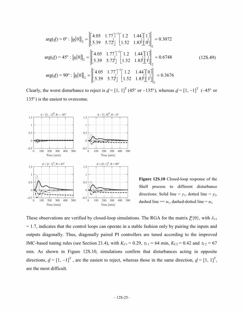
For d = [1,−1]T ,
060601
183152144121
725395771054
0 :45=)arg( 2
1
2 .....
..
..ud =
−
=°−−
(12S.48)
and for three other disturbance directions,
– 12S-25–
3676010
83152144121
725395771054
0 :90=)arg(
6748011
83152144121
725395771054
0 :45=)arg(
3072001
83152144121
725395771054
0 :0=)arg(
2
1
2
2
1
2
2
1
2
.....
..
..ud
.....
..
..ud
.....
..
..ud
=
=°
=
=°
=
=°
−
−
−
(12S.49)
Clearly, the worst disturbance to reject is d = [1, 1]T (45° or −135°), whereas d = [1, −1]T (−45° or
135°) is the easiest to overcome.
Figure 12S.10 Closed-loop response of the
Shell process to different disturbance
directions: Solid line = y1, dotted line = y2,
dashed line == u1, dashed-dotted line = u2.
These observations are verified by closed-loop simulations. The RGA for the matrix P0, with λ11
= 1.7, indicates that the control loops can operate in a stable fashion only by pairing the inputs and
outputs diagonally. Thus, diagonally paired PI controllers are tuned according to the improved
IMC-based tuning rules (see Section 21.4), with KC1 = 0.29, τI 1 = 64 min, KC2 = 0.42 and τI 2 = 67
min. As shown in Figure 12S.10, simulations confirm that disturbances acting in opposite
directions, d = [1, −1]T , are the easiest to reject, whereas those in the same direction, d = [1, 1]T,
are the most difficult.
– 12S-26–
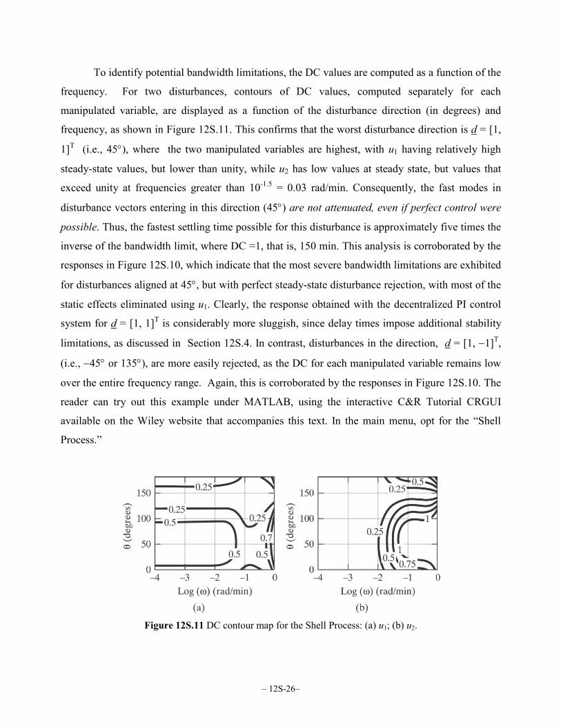
To identify potential bandwidth limitations, the DC values are computed as a function of the
frequency. For two disturbances, contours of DC values, computed separately for each
manipulated variable, are displayed as a function of the disturbance direction (in degrees) and
frequency, as shown in Figure 12S.11. This confirms that the worst disturbance direction is d = [1,
1]T (i.e., 45°), where the two manipulated variables are highest, with u1 having relatively high
steady-state values, but lower than unity, while u2 has low values at steady state, but values that
exceed unity at frequencies greater than 10-1.5 = 0.03 rad/min. Consequently, the fast modes in
disturbance vectors entering in this direction (45°) are not attenuated, even if perfect control were
possible. Thus, the fastest settling time possible for this disturbance is approximately five times the
inverse of the bandwidth limit, where DC =1, that is, 150 min. This analysis is corroborated by the
responses in Figure 12S.10, which indicate that the most severe bandwidth limitations are exhibited
for disturbances aligned at 45°, but with perfect steady-state disturbance rejection, with most of the
static effects eliminated using u1. Clearly, the response obtained with the decentralized PI control
system for d = [1, 1]T is considerably more sluggish, since delay times impose additional stability
limitations, as discussed in Section 12S.4. In contrast, disturbances in the direction, d = [1, −1]T,
(i.e., −45° or 135°), are more easily rejected, as the DC for each manipulated variable remains low
over the entire frequency range. Again, this is corroborated by the responses in Figure 12S.10. The
reader can try out this example under MATLAB, using the interactive C&R Tutorial CRGUI
available on the Wiley website that accompanies this text. In the main menu, opt for the “Shell
Process.”
Figure 12S.11 DC contour map for the Shell Process: (a) u1; (b) u2.
– 12S-27–
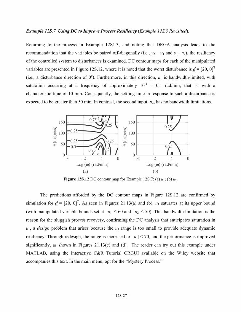
Example 12S.7 Using DC to Improve Process Resiliency (Example 12S.3 Revisited).
Returning to the process in Example 12S1.3, and noting that DRGA analysis leads to the
recommendation that the variables be paired off-diagonally (i.e., y2 – u1 and y1– u2), the resiliency
of the controlled system to disturbances is examined. DC contour maps for each of the manipulated
variables are presented in Figure 12S.12, where it is noted that the worst disturbance is d = [20, 0]T
(i.e., a disturbance direction of 0o). Furthermore, in this direction, u1 is bandwidth-limited, with
saturation occurring at a frequency of approximately 10-1 = 0.1 rad/min; that is, with a
characteristic time of 10 min. Consequently, the settling time in response to such a disturbance is
expected to be greater than 50 min. In contrast, the second input, u2, has no bandwidth limitations.
Figure 12S.12 DC contour map for Example 12S.7: (a) u1; (b) u2.
The predictions afforded by the DC contour maps in Figure 12S.12 are confirmed by
simulation for d = [20, 0]T. As seen in Figures 21.13(a) and (b), u1 saturates at its upper bound
(with manipulated variable bounds set at | u1| ≤ 60 and | u2| ≤ 50). This bandwidth limitation is the
reason for the sluggish process recovery, confirming the DC analysis that anticipates saturation in
u1, a design problem that arises because the u1 range is too small to provide adequate dynamic
resiliency. Through redesign, the range is increased to | u1| ≤ 70, and the performance is improved
significantly, as shown in Figures 21.13(c) and (d). The reader can try out this example under
MATLAB, using the interactive C&R Tutorial CRGUI available on the Wiley website that
accompanies this text. In the main menu, opt for the “Mystery Process.”

– 12S-28–
Figure 12S.13 Closed-loop response with
off-diagonal PI control to the disturbance d
= [20, 0]T for Example 12S.7, with: (a,b)
Original bounds on u1; (c,d) Enlarged
bounds on u1 (to ±70). Shown on the top
row are outputs: y1 (solid line), y2 (dashed
line), and on the bottom row, inputs: u1
(solid line), u2 (dashed line).
12S.3 TOWARD AUTOMATED FLOWSHEET C&R DIAGNOSIS
This section describes a procedure for assessing the controllability and resiliency of a
process flowsheet that relies on heuristics to create a linearized dynamic model of the process using
the results of steady-state simulations. The derived model is used to test the flowsheet C&R, using
the measures introduced in Section 12S.2. As a tutorial exercise, the procedure is applied to screen
the designs for the heat-integrated distillation columns in Example 12.2. Subsequently, in Section
12S.5, case studies are presented for three additional processes. For each case, the results of the
approximate linear analysis are compared with the results of closed-loop simulations using
nonlinear dynamic models. As will be shown, the overall approach is very promising as a short-cut
diagnostic and screening tool, which can be expected to be integrated into commercial simulation
software.
Short-Cut C&R Diagnosis
As discussed above, both steady-state and dynamic C&R analyses provide useful
information for flowsheet assessment. Clearly, the second alternative provides more information
– 12S-29–
and is more reliable. On the other hand, steady-state analysis requires much less work, and is often
adequate for screening purposes. Consequently, both approaches are considered in this section.
The following steps are involved in steady-state analysis:
1. After the flowsheet is synthesized, the control structure is considered, first by selecting the
process outputs to be controlled, yt, the manipulated variables, ut, and the disturbance
variables, dt. These are related by Eq. (12S.1).
2. Steady-state simulation of the flowsheet is carried out using a process simulator.
3. Steady-state gains for the overall transfer functions, 0P and 0dP , are computed by
perturbing each input, one at a time.
4. Steady-state C&R measures are computed using 0P and 0dP .
For the dynamic C&R analysis (Weitz and Lewin, 1996), the steps in the algorithm are as
follows:
1. Step 1 of the steady-state algorithm.
2. Step 2 of the steady-state algorithm.
3. The flowsheet is decomposed into component parts. These are MIMO subsections of the
flowsheet that are approximated by matrices of low-order transfer functions (usually first
order with dead time). This decomposition permits process units to be modeled in sufficient
detail, allowing inverse response and overshoot phenomena to be represented.
4. Steady-state gains for the component parts are computed by perturbation of each input, one
at a time.
5. Time constants and delay times are estimated assuming perfect mixing or plug flow, as
appropriate, with the flow rates at steady state. At this point, transfer function matrices are
defined for each component part.
6. The transfer function matrices, sP and sPd , are generated for the complete flowsheet.
This involves computing the frequency response of each component part, and recombining
the component parts, as dictated by the plant topology.
7. The frequency-dependent C&R measures are computed using the approximate linear model,
P jω and ωjPd .
– 12S-30–
Many packages are available for steady-state simulation, as discussed in Chapter 5. To
manipulate the linearized models in the Laplace, frequency, and time domains, MATLAB and
SIMULINK are used commonly, and example scripts are introduced in Section 12S.6. The most
recent commercial packages permit steady-state and dynamic simulations. These include ASPEN
HYSYS, UNISIM and Aspen Dynamics, with the former used in Sections 12S.3 and 12S.5.
All of the steps in the two algorithms are implemented using an array of computer packages
that are becoming more integrated. Note that steps 4 and 5 deserve special attention, as they are the
basis for the approximate models generated for the dynamic C&R analysis.
Generating Low-Order Dynamic Models
The linearized model for each component part, to be completed in steps 4 and 5 of the
dynamic C&R analysis, has the form
susKsy ccc ⋅Ψ⊗= c (12S.50)
where ucs and ycs are m-dimensional input and n-dimensional output vectors, in complex
space, K c is a matrix of steady-state gains in n× m real space, and scΨ is a matrix describing the
dynamics in n×m complex space (each element of which is typically a delayed, low-order transfer
function with dead time). The term ⊗ denotes the Schur (or element-by-element) product. Each
distillation column is characterized by a single time constant. For heat exchangers, separate time
constants are associated with the tube- and shell-side fluids. In the subsections that follow, it is
shown that the gains, time constants, and dead times can be estimated almost entirely using the
results of steady-state simulations.
Steady-State Gain Matrix, K c
The steady-state gains between the inputs and outputs for each component part are
generated using the following procedure:
1. The material and energy balances, in the steady state, are solved for the complete flowsheet
at the nominal operating point.
2. Small positive and negative perturbations are introduced for each input of each component
part, one at a time, and the changes in the outputs are computed.

– 12S-31–
3. The steady-state gains for each component part are computed using finite differences: Kcij =
∆yci/∆uc
j, where the perturbation, ∆ucj, is sufficiently small to avoid precision losses.
Dynamics Matrix, Ψ c s
In this section, an approach is suggested for estimating the time constants and delay times
for distillation columns and heat exchangers.
Distillation Columns.
Time constants. Following Skogestad (1987), the dominant time constant is estimated as
I C Rτ = τ + τ + τ (12S.51)
where τC and τR are the time constants (in minutes) associated with the condenser and reboiler,
respectively, and τI is the time constant (in minutes) for the column, estimated according to
1
Ni
Iii
ML=
τ =∑ (12S.52)
where Mi is the volumetric holdup (m3) on tray i, Li is the liquid flow rate (m3/min) from tray i, and
N is the number of trays. The liquid holdup is expressed as
( ) ( )owwc
owwci hhDhhAM +=+=4
2π (12S.53)
where Dc is the column diameter (m), and hw and how are the weir height and fluid height above the
weir (m), respectively. The latter can be expressed in terms of the weir length, lw (m), using the
Francis weir equation: 32
111
⋅
=w
iow l
Lh (12S.54)
Delay times. When the internal liquid flow rate in the column changes, a delay time is associated
with the change in the fluid holdup above the weir. For a single tray, this is estimated by
considering the time taken for how to stabilize after a change in the liquid flow rate (Shinskey,
1984): 2
0.5666ow ow c
ci i w ow
dM dt dh DAdL dt dL l h
πθ = = =
⋅ ⋅ (12S.55)
Thus, the overall delay experienced by the bottoms product after changes in the flow rates,
temperatures, or compositions of the feed or reflux depends on the number of trays involved. In

– 12S-32–
contrast, it is noted that the distillate composition responds immediately to a change in the reflux
flow rate, but experiences a considerable delay after changes in the feed concentration or
temperature. For the latter, the delay time is estimated as the sum of the residence times on all trays
between the feed and the top tray, since such a change is assumed to propagate by affecting the
entire tray holdup rather than just the over-weir fluid.
Typical design parameters. The following heuristics are in common use: τC = τR = 0.5τI , lw =
0.65Dc and hw = 2 in.
Heat Exchangers.
It is assumed that time delays associated with heat exchangers in the major processing units,
such as the condensers and reboilers in distillation columns, are negligible. When heat exchangers
are not included in the major processing units, they are modeled as first-order lags associated with
single shell and single tube passes.
Time constants. These are estimated for the tube- and shell-side fluids using τT = VT /qT and τS =
VS /qS. The volumes of the fluid holdups in the tubes and shell, VT and VS, are estimated using the
heat transfer area, the average fluid velocity in the tubes, v, and the tube and shell diameters. The
volumetric flow rates, qT and qS, are estimated by the process simulator.
Example 12S.8: C&R Analysis for Heat-Integrated Distillation Columns (Example 12.2
Revisited)
Dynamic C&R analysis is applied to screen the heat-integrated distillation configurations for the
dehydration of methanol in Figure 12.2 of Example 12.2. Of the three heat-integrated designs, the
FS and LSR configurations provide the maximum energy savings. Clearly, the most controllable
and resilient of the two should be selected based on C&R screening. Note that Chiang and Luyben
(1988) prepared nonlinear dynamic models of the three heat-integrated configurations. They carried
out C&R analysis, using the RGA and minimum singular values, based on linear approximations to
their dynamic models. Although their findings using linear analysis were inconclusive, they
showed the FS configuration to be far less desirable using closed-loop simulations with their
nonlinear models.
– 12S-33–
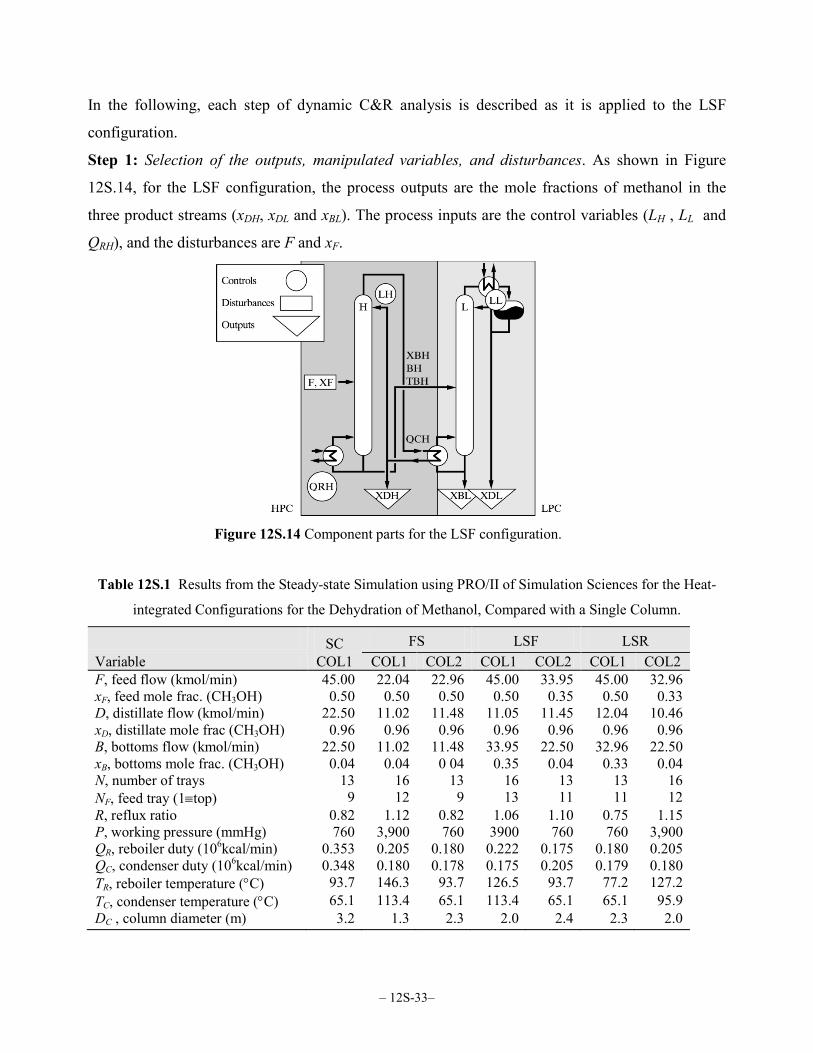
In the following, each step of dynamic C&R analysis is described as it is applied to the LSF
configuration.
Step 1: Selection of the outputs, manipulated variables, and disturbances. As shown in Figure
12S.14, for the LSF configuration, the process outputs are the mole fractions of methanol in the
three product streams (xDH, xDL and xBL). The process inputs are the control variables (LH , LL and
QRH), and the disturbances are F and xF.
Figure 12S.14 Component parts for the LSF configuration.
Table 12S.1 Results from the Steady-state Simulation using PRO/II of Simulation Sciences for the Heat-
integrated Configurations for the Dehydration of Methanol, Compared with a Single Column.
SC FS LSF LSR Variable COL1 COL1 COL2 COL1 COL2 COL1 COL2 F, feed flow (kmol/min) 45.00 22.04 22.96 45.00 33.95 45.00 32.96 xF, feed mole frac. (CH3OH) 0.50 0.50 0.50 0.50 0.35 0.50 0.33 D, distillate flow (kmol/min) 22.50 11.02 11.48 11.05 11.45 12.04 10.46 xD, distillate mole frac (CH3OH) 0.96 0.96 0.96 0.96 0.96 0.96 0.96 B, bottoms flow (kmol/min) 22.50 11.02 11.48 33.95 22.50 32.96 22.50 xB, bottoms mole frac. (CH3OH) 0.04 0.04 0 04 0.35 0.04 0.33 0.04 N, number of trays 13 16 13 16 13 13 16 NF, feed tray (1≡top) 9 12 9 13 11 11 12 R, reflux ratio 0.82 1.12 0.82 1.06 1.10 0.75 1.15 P, working pressure (mmHg) 760 3,900 760 3900 760 760 3,900 QR, reboiler duty (106kcal/min) 0.353 0.205 0.180 0.222 0.175 0.180 0.205 QC, condenser duty (106kcal/min) 0.348 0.180 0.178 0.175 0.205 0.179 0.180 TR, reboiler temperature (°C) 93.7 146.3 93.7 126.5 93.7 77.2 127.2 TC, condenser temperature (°C) 65.1 113.4 65.1 113.4 65.1 65.1 95.9 DC , column diameter (m) 3.2 1.3 2.3 2.0 2.4 2.3 2.0

– 12S-34–
Figure 12S.15 Information flows between the component parts
of the heat-integrated distillation configurations: (a) FS; (b) LSF; (c) LSR.
Step 2: Steady-state simulation. The simulation was carried out using the PRO/II simulator and
assuming that there is no pressure drop in the columns, no heat losses to the surroundings, and tray

– 12S-35–
efficiencies of 75%. The thermodynamic properties were computed using the UNIFAC option.
These conditions were used by Chiang and Luyben (1988), with the exception that they accounted
for heat losses. The results for the four flowsheets are in Table 12S.1. Note that the energy
requirements for the LSR and FS configurations are the lowest (0.205×10⁶ kcal/min), followed by
the LSF configuration (0.222×10⁶ kcal/min).
Step 3: Decomposition into component parts. It has been demonstrated that a first-order lag is a
reasonable approximation for the dynamics of a distillation column (Skogestad, 1987). Thus, the
LSF configuration is decomposed into two component parts, one for each column. Four
intermediate variables are identified to model the information transfer between the component
parts: xBH, BH, TBH and QCH (= −QRL). Note that both TBH and QCH are needed for the energy
balance in the reboiler because partial vaporization occurs.
The control variables, in perturbation variable form, are scaled between zero and their
nominal values, and the disturbances are scaled using bounds 20% above and below their nominal
values. The outputs are scaled to provide a reasonable match with the steady-state gains computed
by Chiang and Luyben (1988), it being noted that the output scaling does not affect the RGA or the
DC values.
Steps 4 and 5: Computing Kc and ψc(s). These are computed following the procedure in the section
on “Generating Low-order Dynamic Models,” which gives linearized models for the high-pressure
column in the LSF configuration:
=
−−−−−
−−−−−−−−−−−
−−−−−−
+
F
RH
H
s.e.s.e..s.ee
s.e.s.e..s.e.
s.e.s.e..s.e.
s.e.s.e..s.e.
s.e....
s
CH
H
BH
BH
DH
xF
QL
QBTxx
10003010001099403154
100201012717123319160
100541102005931330
1029611000608591310110
460900001010910170
1131 (12S.56)
and for the low-pressure column:
=
−−−
−−−−−−
+
L
RL
H
BH
BH
....s.e.
s.e..s.e.s.e.s.e.sDL
BL
LQBTx
xx
0380291300300510587900
4101201612100070100290107920117
1 (12S.57)

– 12S-36–
Step 6: Generation of transfer function matrices. The linear approximation for the flowsheet
dynamics is obtained by recombining the models for the component parts. Note that Figure 12S.15
shows schematically how the linearized models for the component parts are linked in each of the
configurations. The inputs and outputs associated with each of the configurations are represented
by the terminal junctions to the left and right. Thus, for example, the FS configuration has four
manipulated and two disturbance variables (six inputs in all), and four output variables. The blocks
marked HPC and LPC represent the component parts for the high- and low-pressure distillation
columns, respectively. The arcs represent the flow of information (intermediate variables) to and
from the component parts.
The recombination to form overall transfer functions is accomplished by algebraic
manipulation. For the LSF configuration, Eqs. (12S.56) and (12S.57) are rewritten in block-matrix
form:
( ) ( )( ) ( )
=
F
RH
H
,P,P
,P,P
CH
H
BH
BH
DH
xF
QL
QBTxx
HH
HH
2212
2111 (12S.58)
( ) ( )[ ]
=
L
RL
H
BH
BH
,P,PDL
BL
LQBTx
xx
LL 2111 (12S.59)
where the matrix blocks contain elements from the transfer function matrices in Eqs. (12S.56) and
(12S.57); for example,
( ) [ ]10910170113
111 ..
s,PH −=
+
Next, by algebraic manipulation, the vector of internal variables, namely [xBH TBH BH QCH]T, is
eliminated, leading to
[ ] ( ) ( )x PL
QL
P FxDH H
HRHL
H F=
+
11 0 1 2, , (12S.60)

– 12S-37–
( ) ( ) ( ) ( ) ( )xx P P P
LQL
P P Fx
BLDL L H L
HRHL
L H F
= ⋅
+ ⋅
11 2 1 1 2 11 2 2, , , , , (12S.61)
Note that Eqs. (12S.60) and (12S.61) are in the standard transfer function form of Eq. (12S.1).
Similar manipulations are used for the other two configurations. The LSR configuration involves
the most complicated manipulations, since it involves the feedback of information.
These models are compared with those derived by Chiang and Luyben (1988), who fitted
linear transfer functions to the transient open-loop responses that were computed using their
nonlinear model. In Figure 12S.16, the diagonal RGA matrix coefficients for all four configurations
are plotted against the frequency; the values reported by Chiang and Luyben appear on the right,
while those computed using the linear models derived using the C&R analysis appear on the left.
As shown, the results are in close agreement. The resonant peaks computed by Chiang and Luyben
are the result of differences in the time constants and delay times in the transfer function elements.
Furthermore, the relative gains, computed using the procedure in this section, do not vary
significantly with frequency. Hence, diagonal pairings are preferred for the decentralized control
system.
Step 7: Computation of C&R measures. Figure 12S.17 shows the DC contour maps computed for
each of the manipulated variables associated with the configurations SC, LSR, and FS, where the
ordinate is the direction of the disturbance [F, xF]T, and the abscissa is the log 10 of the frequency.
Since DC values in excess of unity correspond to saturated manipulated variables, it is apparent that
the disturbances are rejected adequately by all of the designs at the steady state (i.e., when ω = 0).
However, for a wide range of disturbance directions, the FS configuration has disturbance costs in
excess of unity at frequencies beyond 0.1 rad/min in three of the manipulated variables (LH, QRH
and FH/FL). Thus, disturbance rejection is expected to be very sluggish for this configuration. The
other two configurations have low disturbance costs, and are expected to reject these disturbances
nearly as well as a single column. Thus, the FS configuration should be rejected and the LSR
configuration selected, because its energy requirements are lower than for the LSF and SC
configurations.

– 12S-38–
Figure 12S.16 Diagonal RGA elements as a function of frequency for the four configurations to dehydrate
methanol: (a) Procedure in Section 12S.3; (b) Chiang and Luyben (1988).
To confirm these results, nonlinear dynamic simulations are carried out using HYSYS.
Three configurations are simulated: (1) the single column (SC) in the LV configuration; (2) the FS
configuration with the pairing: xDH –LH, xBH – QRH, xDL –LL and xBL –FH/FL ; (3) the LSR

– 12S-39–
configuration with the pairing: xDH –LH, xBH – QRH and xDL –LL. These pairings are selected on the
basis of the RGA. The control loops tuned using the IMC-PI tuning rules (see Section 12S.4), with
tuning parameters summarized in Table 12S.2. Note that the nominal values of the manipulated
variables are at the mid-point of their ranges.
Figure 12S.17 DC contour maps for the SC, FS and LSR configurations to dehydrate methanol. The bounds
on the disturbances are ±20% from their nominal values. The DC contour maps for each
manipulated variable are computed separately, with bold solid lines indicating DC = 1. See
Figure 12S.39 for the DC contour maps for the LSF configuration.

– 12S-40–
Table 12S.2: Tuning parameters for the SC, LSR and FS Configurations.
Loop SC† LSR FS
xDL –LL Kc = 29; τI = 10 min Kc = 1; τI = 10 min Kc = 1; τI = 5 min
xBL – QRL Kc = 6; τI = 10 min
xBL – FH/FL‡ Kc = 0.5; τI = 30 min
xDH –LH Kc = 0.15; τI = 5 min Kc = 1; τI = 5 min xBH – QRH Kc = 1; τI = 10 min Kc = 0.1; τI = 10 min
Notes: † For the SC configuration, the temperatures on trays 2 and 10 are regulated instead of the
compositions.
‡ The xBL composition controller is the master of a lower-level flow controller to regulate
FH/FL.
Figures 21.18, 21.19 and 21.20 show the responses for the three configurations, subjected to
the worst-case disturbance in which the feed flow rate and composition simultaneously undergo
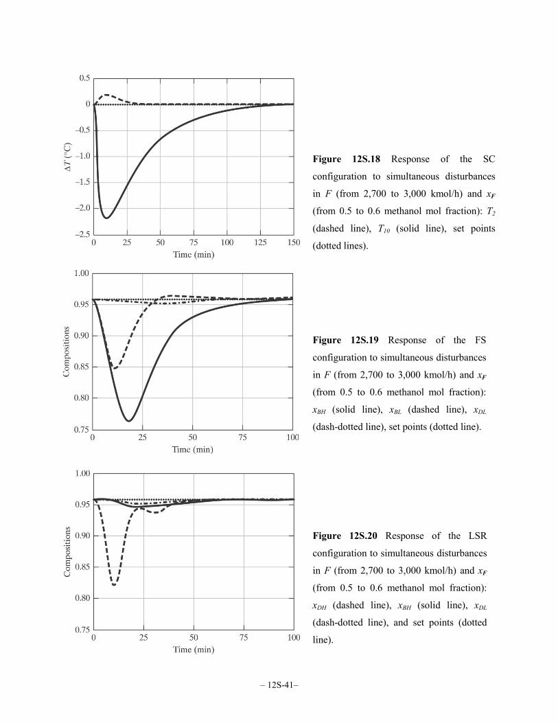
positive step changes to their design limits. As shown in Figure 12S.18, the SC configuration is
returned to its set points in approximately 100 min, with T10 most affected. Note that this response
is qualitatively similar to that of the linear approximation shown in Figure 12S.3. The simulation
can be reproduced using the METH_SC.HSC file available on the Wiley web site that accompanies
this book.
As shown in Figure 12S.19, the response of the FS configuration to the same disturbance is
very sluggish, settling in about 100 minutes, and exhibiting severe undershoots in two of the four
mole fractions: xBH (by 20 mol %) and xBL (by 10 mol %). This verifies the predictions of the DC
contour maps in Figure 12S.17, which anticipate significant bandwidth limitations. These
simulation results can be reproduced using the METH_FS.HSC file, also available on the Wiley
web site.
– 12S-41–
Figure 12S.18 Response of the SC
configuration to simultaneous disturbances
in F (from 2,700 to 3,000 kmol/h) and xF
(from 0.5 to 0.6 methanol mol fraction): T2
(dashed line), T10 (solid line), set points
(dotted lines).
Figure 12S.19 Response of the FS
configuration to simultaneous disturbances
in F (from 2,700 to 3,000 kmol/h) and xF
(from 0.5 to 0.6 methanol mol fraction):
xBH (solid line), xBL (dashed line), xDL
(dash-dotted line), set points (dotted line).
Figure 12S.20 Response of the LSR
configuration to simultaneous disturbances
in F (from 2,700 to 3,000 kmol/h) and xF
(from 0.5 to 0.6 methanol mol fraction):
xDH (dashed line), xBH (solid line), xDL
(dash-dotted line), and set points (dotted
line).

– 12S-42–
In contrast, the response of the LSR configuration to the same disturbance, shown in Figure
12S.20, settles in about half the time, with significantly less undershoot in xDL. This is because the
controllers are significantly less bandwidth-limited, as predicted by the DC contour maps in Figure
12S.17. Furthermore, the settling time of the LSR configuration is comparable to that for the single
column, as predicted by the DC analysis. These simulation results can be reproduced using the
METH_LSR.HSC file on available on the Wiley web site.
It should be emphasized that the DC contour maps are based on the assumption of perfect
control, assuming that there are no stability limitations to increases in the controller gain. In
practice, when single-loop controllers are implemented, the controller gains are limited, as in this
example, by process interactions, or by single-loop stability limitations such as delay times. As a
result, the bandwidth limitations are usually underestimated by the DC contour maps, but usually
not sufficiently to affect their diagnoses when used to screen alternative designs. Note that the
prediction that the FS configuration provides significantly worse disturbance rejection compared
with that of the LSR configuration has been verified by simulation. Clearly, the LSR design is
preferable based on energy-efficiency and controllability.
This approach has been used successfully for screening more complex heat-integrated
flowsheets (Weitz, 1994), exothermic reactors (Naot and Lewin, 1995), and polymerization
reactors (Lewin and Bogle, 1996). In all cases, the projections were confirmed using rigorous
dynamic models. To further illustrate this screening technique, Section 12S.5 provides three case
studies, involving exothermic reactors in series, heat-exchanger networks, and a recycle process.

– 12S - 43 –
12S.4 CONTROLLER LOOP DEFINITION AND TUNING
Since the regulatory loops use PI controllers for verification of the C&R analysis, a brief summary
of their configuration and tuning is provided in this section.
Definition of PID Control Loop.
This involves specifying:
1. The process variable to be controlled, PV; that is, any stream- or operation-related variable
in the flowsheet (e.g., pressure, temperature, liquid level, species mass or mole fraction,
mass or molar flow rate). The minimum and maximum values of the PV are used to express
the PV as a percentage of its full range:
( )PVPV PV
PV PV% min
max min=
−−
×100 (12S.62)
2. The controller output, OP, to be manipulated by the controller, as a percentage of its full
range. This variable is usually either a stream flow rate or the rate of heat transfer of an
energy stream. Generally, its minimum value is specified as zero and its maximum is taken
as twice its nominal value. Note that occasionally the nominal value is not positioned
midway between the minimum and maximum values (e.g., when the nominal flow rate of a
bypass stream lies near its maximum or minimum flow rate).
3. The controller action, either direct or reverse acting, which defines the direction of its
effect. For a direct-acting controller, when the PV rises above the setpoint (SP), the OP
increases, and vice versa. In these cases, the static process gain is negative, as illustrated for
a level controller in Figure 12S.21(a). Here, the liquid level is the PV, the flow rate of the
effluent stream, Qo, is the OP, and the controller action is set to Direct. In contrast, for a
reverse-acting controller, when the PV rises above the SP, the OP decreases, and vice versa.
In these cases, the static process gain is positive, as illustrated in Figure 12S.21(b), which
shows a different controller configuration for the surge tank. Here, the flow rate of the feed
stream, Qi, is the OP, and the controller action is set to reverse.

– 12S - 44 –
Figure 12S.21 Level-control configurations for a surge tank:
(a) Direct acting; (b) Reverse acting
4. The tuning parameters. For a PID controller, the output, OP(t), is a function of the tracking
error, E(t):
τ+θθ
τ++= ∫ dt
tdEdEtEKOPtOP dt
iCSS 0
1 (12S.63)
where OPSS is the bias, or controller output at zero error, and KC, τi and τd are the
proportional gain, integral time constant (or reset time), and derivative time constant (or rate
time) of the controller. The tracking error at time t, E(t), is the difference between the set
point and the process variable:
tPVtSPtE −= (12S.64)
As mentioned above, SP, PV and OP are expressed as percentages of their full ranges.
Consequently, the controller gain, KC, is dimensionless, and represents the percentage
change in OP for a one-percent change in PV. In the absence of other information, factory
settings are used: KC = 1, τi = 10 min. and τd = 0. These are tuned for improved
performance, as discussed in the next section.
Controller Tuning.
The PID (Proportional-Integral-Derivative) controller is the most commonly used feedback
controller in industry, with three tunable parameters as stated previously. The integral component
ensures that the tracking error, Et, is asymptotically reduced to zero, whereas the derivative
component imparts a predictive capability, potentially enhancing the performance. Despite its
apparent simplicity, the subject of PID controller tuning has been discussed in several textbooks
and thousands of research papers since the landmark work of Ziegler and Nichols (1942). In

– 12S - 45 –
practice, despite these developments, most PID controllers are tuned as PI controllers for several
reasons.
1. The improved performance attainable using the derivative term is often not required. In
many cases, the derivative action causes the controller to respond more nervously,
especially when step changes are imposed on the set points. Furthermore, as pointed out by
Luyben and coworkers (1999), it is often sufficient to tune level controllers as proportional-
only regulators (i.e., 1/τi = 0 and τd = 0).
2. The derivative component amplifies measurement noise. It is highly recommended that
derivative action be applied only to filtered feedback signals.
3. Using model-based tuning methods, as discussed in the section on “Model-based PI
Controller Tuning,” higher-order models are needed to tune a PID controller. In many cases,
the additional engineering effort is not justified.
4. Many PID controller loops remain on their factory settings long after plant start-up. When
the controller action is in the right direction and the PV range is defined wisely, these
settings often give adequate performance.
For tuning, either on-line methods, implemented with controllers on-line, or model-
based methods, which rely on process models, are utilized. The main advantages of the on-line
methods are that tuning occurs under closed-loop control and a process model is not required. It
should be recognized, however, that they provide initial controller settings that are usually
improved iteratively during operation. Furthermore, typical on-line tuning rules apply strictly
for a single control loop. For a multivariable control system, detuning is often necessary to
prevent process interactions from introducing instability. Because no guidelines are available to
modify the controller parameters when this occurs, the discussion below focuses on model-
based PI tuning rules. For more details on on-line tuning, the reader is referred to Seborg et al.
(1989), Luyben (1990), and the section covering process dynamics on the multimedia on the
Wiley website that accompanies this text (HYSYS → Dynamic Simulation → Tuning PI
Controllers).
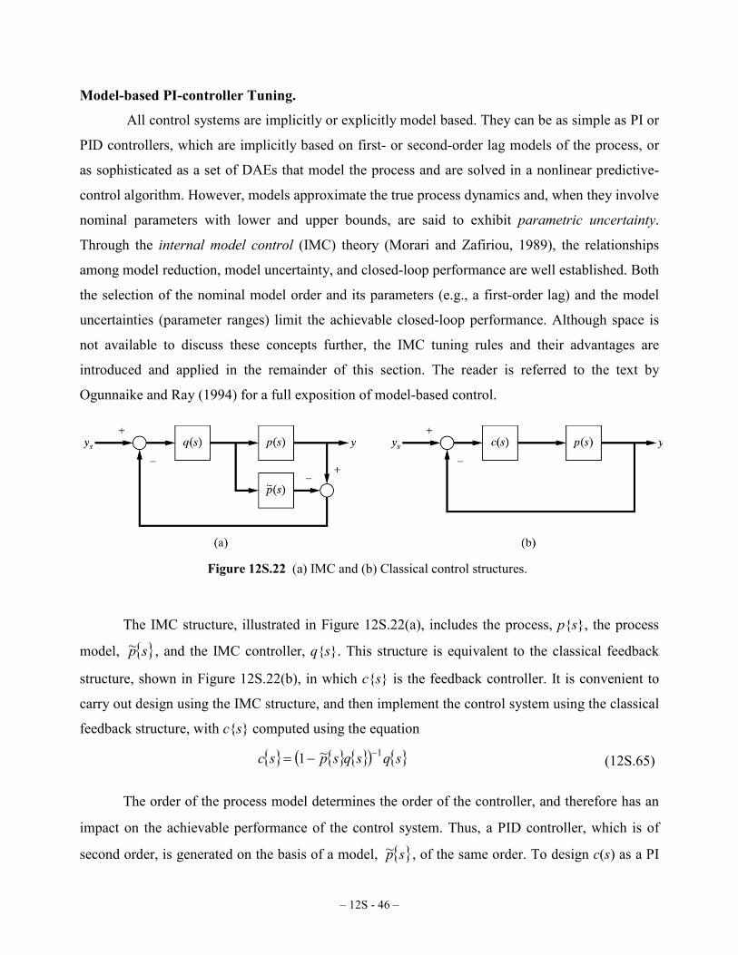
– 12S - 46 –
Model-based PI-controller Tuning.
All control systems are implicitly or explicitly model based. They can be as simple as PI or
PID controllers, which are implicitly based on first- or second-order lag models of the process, or
as sophisticated as a set of DAEs that model the process and are solved in a nonlinear predictive-
control algorithm. However, models approximate the true process dynamics and, when they involve
nominal parameters with lower and upper bounds, are said to exhibit parametric uncertainty.
Through the internal model control (IMC) theory (Morari and Zafiriou, 1989), the relationships
among model reduction, model uncertainty, and closed-loop performance are well established. Both
the selection of the nominal model order and its parameters (e.g., a first-order lag) and the model
uncertainties (parameter ranges) limit the achievable closed-loop performance. Although space is
not available to discuss these concepts further, the IMC tuning rules and their advantages are
introduced and applied in the remainder of this section. The reader is referred to the text by
Ogunnaike and Ray (1994) for a full exposition of model-based control.
Figure 12S.22 (a) IMC and (b) Classical control structures.
The IMC structure, illustrated in Figure 12S.22(a), includes the process, ps, the process
model, sp~ , and the IMC controller, qs. This structure is equivalent to the classical feedback
structure, shown in Figure 12S.22(b), in which cs is the feedback controller. It is convenient to
carry out design using the IMC structure, and then implement the control system using the classical
feedback structure, with cs computed using the equation
( ) sqsqsp~sc 11 −−= (12S.65)
The order of the process model determines the order of the controller, and therefore has an
impact on the achievable performance of the control system. Thus, a PID controller, which is of
second order, is generated on the basis of a model, sp~ , of the same order. To design c(s) as a PI

– 12S - 47 –
controller, the process model is limited to a first-order transfer function: ( ) 11 −+τ= sKsp~ p , in
which case the IMC controller becomes ( )( ) 1111 −−+λ+τ= pKsssq , where λ is the time constant
of the IMC filter. Using Eq. (12S.65), the classical feedback controller is
( ) ( )( )
τ+≡λ+τ=−= −−
sKsKssqsqsp~sc
iCp
1111 11 (12S.66)
By equivalence of the terms, the IMC-PI tuning rules are
τi = τ and λτ PiC KK = . (12S.67)
For processes exhibiting time delay, e.g., ( ) 11 −θ− +τ= seKsp~ sp , Rivera et al. (1986) recommend
the IMC tuning rules:
λτττ θPiCi KK =+= and
2. (12S.68)
IMC-based tuning parameters have been computed for a variety of open-loop stable transfer
functions by Rivera et al. (1986), and for open-loop unstable transfer functions by Rotstein and
Lewin (1991). The main advantage of the IMC tuning rules is that the time constant of the IMC
filter is the only tunable parameter. This is of great practical importance because it provides
guidance for detuning the controllers in the face of model uncertainty and multivariable system
interactions. The value of λ should be set initially to either the desired closed-loop time constant
(about one-fifth of the desired settling time), or to twice the process delay time, whichever is the
greatest. Increased robustness (less oscillations) is attained by increasing its value, whereas more
aggressive control action results from decreasing its value.
Example 12S.9 Tuning PI Control Loops for a Binary Distillation Column (Example 12S.7
Revisited)
As discussed in Example 12S.8, this column, for the dehydration of methanol, is simulated using
ASPEN HYSYS. To assist in tuning the PI controllers, each control loop is placed in manual
operation and a step change in the manipulated variable is applied. For a step change from 50 to
60% of the maximum reflux flow, the temperature of the second tray (used to regulate the distillate
composition) is reduced from 66.7 to 66 oC, with a settling time of about 50 min. Since the PV
range is defined from 25 to 125 oC, the 10% increase in OP causes a PV change of:
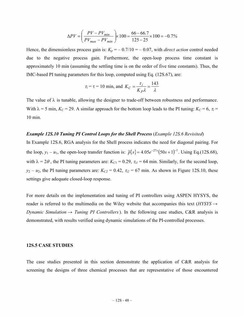
– 12S - 48 –
%..PVPV
PVPVPVminmax
min 7010025125
76666100 −=×−
−=×
−
−=∆
Hence, the dimensionless process gain is: Kp = – 0.7/10 = – 0.07, with direct action control needed
due to the negative process gain. Furthermore, the open-loop process time constant is
approximately 10 min (assuming the settling time is on the order of five time constants). Thus, the
IMC-based PI tuning parameters for this loop, computed using Eq. (12S.67), are:
τi = τ = 10 min, and λλ
τ 143==
P
iC K
K
The value of λ is tunable, allowing the designer to trade-off between robustness and performance.
With λ = 5 min, KC = 29. A similar approach for the bottom loop leads to the PI tuning: KC = 6, τi =
10 min.
Example 12S.10 Tuning PI Control Loops for the Shell Process (Example 12S.6 Revisited)
In Example 12S.6, RGA analysis for the Shell process indicates the need for diagonal pairing. For
the loop, y1 – u1, the open-loop transfer function is: ( ) 127 150054 −− += se.sp~ s . Using Eq.(12S.68),
with λ = 2θ , the PI tuning parameters are: KC1 = 0.29, τi1 = 64 min. Similarly, for the second loop,
y2 – u2, the PI tuning parameters are: KC2 = 0.42, τi2 = 67 min. As shown in Figure 12S.10, these
settings give adequate closed-loop response.
For more details on the implementation and tuning of PI controllers using ASPEN HYSYS, the
reader is referred to the multimedia on the Wiley website that accompanies this text (HYSYS →
Dynamic Simulation → Tuning PI Controllers ). In the following case studies, C&R analysis is
demonstrated, with results verified using dynamic simulations of the PI-controlled processes.
12S.5 CASE STUDIES
The case studies presented in this section demonstrate the application of C&R analysis for
screening the designs of three chemical processes that are representative of those encountered

– 12S - 49 –
during process synthesis. The case studies also show how the results using steady-state and
dynamic C&R analyses compare.
Case Study 12S.1 Exothermic Reactor Design for the Production of Propylene Glycol (Example
12S.1 Revisited)
Returning To Step 1 of Example 12S.1, the CSTR to hydrolyze propylene oxide to propylene
glycol is considered further. Its material and energy balances are in Eq. (12S.6) and (12S.7), with
variables defined and specifications provided. Beginning with these dynamic balances, the steady-
state behavior patterns for this reactor are examined next.
Steady-State Solution
Eq. (12S.8) provides an expression for the PO concentration in the reactor in terms of the reactor
temperature:
ττ
TkCTk
TC in,POPO 2
1 41 −+= (12S.69)
where CPO,in = ℑPO,in/(q0 + qw) and the residence time, τ = V/(q0 + qw). Note that the fractional
conversion of PO is, X = 1 – CPO/CPO,in. Substituting for conversion in Eq. (12S.9), provides
expressions for the heat generation and removal rates in terms of the reactor temperature:
( ) ( )τ
02 1 TTH,HTCTkC
H REMPOP
GEN−
=∆−= (12S.70)
These are monotonically increasing functions of the reactor temperature. HGEN is small at low
temperatures, where the reaction rates are small, rising exponentially with temperature to a plateau
limited by the complete conversion of PO. In contrast, HREM varies linearly with the reactor
temperature. Figure 12S.23 shows these rates as a function of T for qw = 5.325 m3/h. Note that a
steady state occurs at the intersection of the two curves, at T = 82.4 oC, X = 0.97. For small positive
perturbations in temperature in the vicinity of T = 82.4 oC, the heat removal rate is higher than the
heat generation rate, whereas the opposite is true for small negative perturbations. Such imbalances
result in the temperature returning to its operating point, which is referred to as stable in the open
loop or open-loop stable.
– 12S - 50 –
Figure 12S.23 Solution diagram for
PO hydration in a CSTR with
qw = 5.325 m3/h: HGEN = solid line,
HREM = dotted line.
Figure 12S.24 Solution diagram for
PO hydration in a CSTR with qw = 8
m3/h: HGEN = solid line, HREM = dotted
line.
As qw increases, τ decreases shifting HREM to the left, while increasing its gradient. At qw =
8 m3/h, three intersections with the HGEN curve occur, corresponding to three steady-state solutions,
as shown in Figure 12S.24. The upper and lower intersections, at 62 and 25 oC, are stable in the
open loop. However, for small positive perturbations in temperature in the vicinity of T = 44 oC, the
heat removal rate is lower than the heat generation rate. This imbalance causes the reactor to move
to the upper (stable) operating point. Similarly, small negative perturbations in temperature cause
the reactor to move to the lower (stable) operating point. Therefore, the intermediate operating
point is referred to as unstable in the open loop or open-loop unstable. This operating point can

– 12S - 51 –
only be maintained by installing a feedback control system, whose gain must be high enough to
ensure closed-loop stability. The multiplicity of steady states exhibited by the CSTR may lead to
hysteresis phenomena when operating the reactor. This is illustrated using ASPEN PLUS and
ASPEN HYSYS on the multimedia on the Wiley website that accompanies this text. See the
sections on modeling CSTRs.
Returning to the steady state for qw = 5.325 m3/h, a conversion in excess of 95% is obtained
with a 47-ft3 CSTR operating at 85% capacity, which is denoted as the nominal operating point.
Assuming an aspect ratio of L/D = 2, the diameter for a single reactor is D1 = 3.1 ft. Consider an
alternative design composed of two CSTRs in series, as shown in Figure 12S.27b. Assuming
perfect level control by manipulating the effluent streams, two output variables, T1 and T2, are
controlled by two manipulated variables, qw1 and qw2 (the water feed rates). Assuming operation at
approximately the same temperature in each CSTR (about 80 oC), two 14-ft3 CSTRs in series
provide the same conversion as for the base-case design involving a single reactor. Assuming the
reactors are operated at 85% capacity and designed with the same aspect ratio (L/D = 2), the
diameters are D2 = 2.08 ft. Because of the small vessel volumes in both of the alternative designs,
it is not possible to estimate their costs using Eq. (22.54).
C&R Diagnosis
Based on safety considerations, the design involving two CSTRs is preferred, since it involves a
smaller inventory of dangerous reagents. It remains to examine the C&R measures for these two
designs. Beginning with a single CSTR, Eqs. (12S.6) and (12S.7) are linearized, as shown in
Section 21.1, in the vicinity of the steady state to give P(s) and Pd(s) in Eq. (12S.1):
( ) ( ) and 11D
TdU
T BAIsCsPBAIsCsP −− −=−= , (12S.71)
where the scaled state-space matrices are:
−−=
887001644043552039
....
A
−−
=0555007820..
BU
=
00700003302
..
BD [ ]10=C

– 12S - 52 –
These Jacobian matrices can also be computed by making small positive and negative
perturbations in each input variable, one at a time. The perturbation magnitude is reduced until the
magnitude of the resulting change in the outputs is insensitive to the direction of the input
perturbation. The matrices are input scaled, assuming that the manipulated variables are nominally
at 50% of their full range, PO feed rate disturbances (i.e., production rate changes) are limited to
±50% of the nominal value, and feed temperature disturbances are limited to ±5 oC. The time in Eq.
(12S.71) is in minutes.
Using the linear approximation, the DC contour map in Figure 12S.25 identifies the worst
disturbance as ∆d = [+50%, 0 oC]T, that is, throughput changes. Even with this disturbance, the
linear approximation indicates that there are no limitations to perfect disturbance rejection, since all
of the DC values up to a frequency of 10 rad/min lie well below unity.
Figure 12S.25 DC contour map for PO hydration in a single CSTR.
A similar analysis for the two CSTRs in series yields the DC contour maps in Figure
12S.26. While the first reactor has disturbance rejection comparable to that for the single reactor,
the control variable in the second reactor is saturated at steady-state for the worst disturbance
direction (feed rate change alone). Hence, even for perfect control in the second reactor, the
temperature setpoint cannot be maintained for this disturbance. However, this is mitigated by the
fact that the conversion in the second reactor is small, and hence, the offset in T2 is expected to be
small.
– 12S - 53 –
Figure 12S.26 DC contour maps for PO hydration in two CSTRs in series:
(a) DC contour map for qw1; (b) DC contour map for qw 2.
Table 12S.3 Controller Tuning Parameters for the Two Reactor Configurations.
Single CSTR Configuration (see Figure 12S.27a)
Loop PV Range Kc τI, min Action FC-1 0−100 kmol/h 0.1 1 Reverse TC-1 20−120 oC 1.5 4 Direct LC-1 0−100% 1 10 Direct
Two-CSTR Configuration (see Figure 12S.27b) Loop PV Range Kc τI, min Action FC-1 0−100 kmol/h 0.1 1 Reverse TC-1 20−120 oC 0.5 2 Direct TC-2 20−120 oC 3 4 Direct LC-1 0−100% 1 5 Direct LC-2 0−100% 1 5 Direct
– 12S - 54 –
Figure 12S.27 Control configurations for the alternative reactor configurations:
(a) Single CSTR; (b) Two CSTRs in series.
It should be noted that these results assume that perfect control is achievable. Thus, the true
response is expected to be worse than that predicted based on the linear analysis, especially when
single-loop PI controllers are implemented. Based upon the C&R analysis, two CSTRs are
anticipated to provide the same disturbance rejection as obtained with a single CSTR. This suggests
that the former should be selected, since it is the safest design. To confirm this conclusion, dynamic
simulation of both systems is carried out using ASPEN HYSYS. Table 12S.3 summarizes the PI
tuning parameters, with the control configurations shown in Figure 12S.27. The IMC-PI tuning
parameters, computed using the approach described in Section 12S.4, are detuned for the level
control loops, and ensure relatively tight control on the reactor temperatures. Perfect pressures
control is assumed, by adjusting the small flow rates in the vapor vents (3 bar for the first vessel,
and 2 bar for the second). The pressure control loops are not simulated explicitly.

– 12S - 55 –
Figure 12S.28 Response of the single CSTR to 50% positive and negative changes in throughput:
(a) feed rate and set point; (b) reactor temperature; (c) water feed rate (%); (d) Reactor level.
Because the DC analysis indicates that the most challenging regulatory control is associated
with throughput changes, the organic feed rate is adjusted, and closed-loop simulations are
performed to check the effects of positive and negative changes in q0. The response of the single
CSTR is shown in Figure 12S.28, and indicates that both positive and negative throughput changes
of 50% are easily handled, with the reactor temperature returned to its setpoint in about 15 min,
while the coolant flow rate, qw, remains within its constraints, as predicted by the DC analysis. The
response of the liquid level is more sluggish by design. The responses of the two-CSTR system
compare well with that for the single CSTR, as shown in Figure 12S.29. Its response to a positive
feed rate change is rapid, with no evidence of saturation on either manipulated variable. In contrast,
– 12S - 56 –
the coolant flow rate to the second reactor, qw2, saturates in response to a negative change in the
throughput, as predicted by the DC analysis. However, as seen in Figure 12S.29, this does not
significantly affect T2.
Figure 12S.29 Response of the two-CSTR system to 50% positive and negative changes in throughput:
(a) feed flow rate and set point; (b) reactor temperatures (T1 – solid T2 – dashed);
(c) water feed flow rate (qw1 – solid qw2 – dashed, in %); (d) holdups (L1 – solid L2 – dashed).
For more details, the reader is referred to the section covering dynamic simulation with
ASPEN HYSYS on the multimedia available on the Wiley website accompanies this text. The
results in Figures 12S.28 and 12S.29 can be reproduced using the files, CSTR_1.hsc and
CSTR_2.hsc.
– 12S - 57 –
In summary, it would appear that despite indicating potential saturation problems associated
with the more complex two-CSTR system, C&R analysis shows that the dynamic responses of the
two systems are approximately the same. This suggests that the two-CSTR system should be
adopted, since it is the safest. However, designs involving smaller hold-ups are often less resilient,
especially in the face of disturbances that manifest themselves rapidly. This example has focused
on the importance of performing C&R analysis in reactor design. For more examples, the reader is
encouraged to study the following publications:
1. Luyben et al (1999): Chapter 4 discusses the design of control systems for reactors in
general. The design of heat-integrated reactor systems is discussed in Chapter 5.
2. Shinskey (1988): Chapter 10 discusses reactor control in industrial practice.
3. Lewin and Bogle (1996): This paper concerns the optimal operation and controllability
of a continuous polymerization reactor.
4. Russo and Bequette (1998): This paper discusses the multiplicity of steady-states
associated with jacketed polymerization reactors.
Case Study 12S.2 Two Alternative Heat Exchanger Networks (Examples 12.1 and 12.5 Revisited)
Here, the two alternative heat exchanger networks (HENs) in Examples 12.1 and 12.5 are screened
using C&R analysis. More specifically, the two designs are required to be resilient to ±5% changes
in F1 and ±5 oF in T0. As discussed in Chapter 12, it is often necessary to augment the process
degrees-of-freedom to meet control objectives, either by addition of trim utility exchangers, or by
adding bypasses, as is the case here. The focus of this study is in the use of resiliency analysis to
select the design configuration and to adjust its nominal operating conditions.
Original HEN (No Bypass).
In the network shown in Figure 12S.30, only two of the target temperatures, θ2 and θ4, are
controlled by manipulation of the flow rates of the two cold streams, leaving the third target
temperature, T3, uncontrolled. The energy balances for this system involve 15 variables: F1, F2, F3,
T0, T1, T2, T3, θ0, θ1, θ2, θ3, θ4, Q1, Q2 and Q3, two of which, θ0 and θ1, are considered to be fixed,
and two, F1 and T0, are considered to be external disturbances.

– 12S - 58 –
Figure 12S.30 Heat-exchanger network without bypass.
Three energy balances apply for each heat exchanger. For the first heat exchanger, E-100,
they are:
( ) 0101111 =−−= TTCFQxf p (12S.72)
( ) 0343312 =−−= θθpCFQxf (12S.73)
( ) ( )( ) ( )[ ] 0
ln 3140
31401113 =
−−−−−
−=θθθθ
TTTTAUQxf (12S.74)
For E-101, the equations are
( ) 0211124 =−−= TTCFQxf p (12S.75)
( ) 0122225 =−−= θθpCFQxf (12S.76)
( ) ( )( ) ( )[ ] 0
ln 1221
12212226 =
−−−−−
−=θθθθ
TTTTAUQxf (12S.77)
Finally, for E-102,
( ) 0321137 =−−= TTCFQxf p (12S.78)
( ) 0033338 =−−= θθpCFQxf (12S.79)
( ) ( )( ) ( )[ ] 0
ln 0332
03323339 =
−−−−−
−=θθθθ
TTTT
AUQxf (12S.80)
– 12S - 59 –
where Ui and Ai are the heat transfer coefficients and heat transfer areas for exchanger i,
respectively, such that: U1A1 = 0.0811 MMBtu/h oF, U2A2 = 0.3162 MMBtu/h oF, and U3A3 =
0.1386 MMBtu/h oF. The number of independent manipulated variables is NManipulated = NVariables −
NExternally Defined − NEquations = 15 − 4 − 9 = 2, and the pairings can be selected using the RGA. To
accomplish this, a linearized model is generated using the following procedure:
1. The nonlinear state equations, fx = 0, in Eqs. (12S.72)-(12S.80) are solved for the
nominal values of the manipulated variables, u = [F2, F3 ]T, disturbances, d = [F1 ,T0]T,
and constants θ0 and θ1, to determine 9 state variables: x = [T1, T2, T3, θ2, θ3,θ4, Q1, Q2,
Q3]T . This is accomplished using an appropriate numerical method (e.g., the Newton-
Raphson method).
2. The output vector, y = [θ2,θ4]T, is recomputed for small positive and negative
perturbations of magnitude ∆ui to each manipulated variable, ui, one at a time, with the
results stored in the vectors yp,i and yn,i, respectively. Then, column i of the steady-state
gain matrix, P 0, is computed: pji0 = ∆uimax ⋅(yp,i,j − yn,i,j)/∆ui, j = 1,…,3. Note that a
factor of ∆uimax scales the input variables such that ui≤ 1.
3. The output vector is recomputed for small positive and negative perturbations of
magnitude ∆di to each disturbance variable, di, one at a time, with the results stored in
the vectors yp,i and yn,i, respectively. Then, column i of the steady-state gain matrix, Pd
0, is computed: pdji0 = ∆dimax ⋅(yp,i,j − yn,i,j)/∆di, j = 1,…,3. The disturbance gain
matrix is scaled arbitrarily relative to the inputs using the scaling ∆dmax= [5%, 5 oF]T.
Since the nominal values of the manipulated variables are u = [F2, F3 ]T = [1.00, 1.00]T , the
maximum perturbations are ∆umax = [1.00, 1.00]T. The resulting linearized model is:
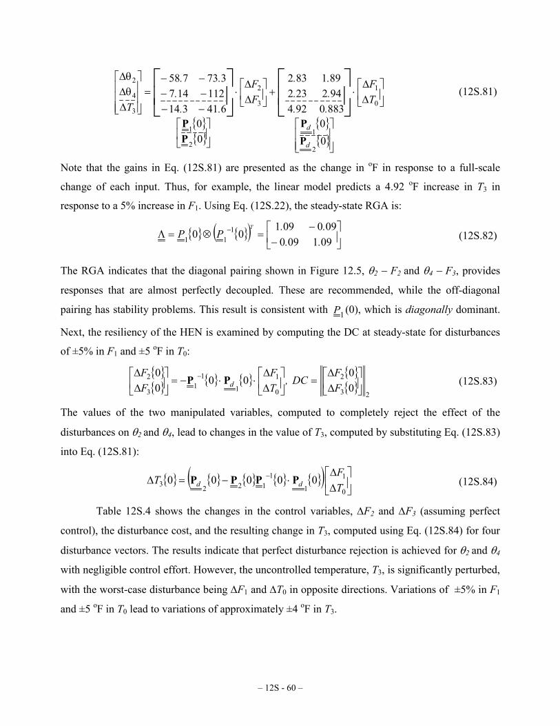
– 12S - 60 –
∆∆
⋅
+
∆∆
⋅
−−−−−−
=
∆θ∆θ∆
0
1
2
1
3
2
2
1
3
4
2
8830924942232891832
00
641314112147
373758
00
TF
......
FF
...
..
T
d
d
PP
PP
(12S.81)
Note that the gains in Eq. (12S.81) are presented as the change in oF in response to a full-scale
change of each input. Thus, for example, the linear model predicts a 4.92 oF increase in T3 in
response to a 5% increase in F1. Using Eq. (12S.22), the steady-state RGA is:
( )
−
−=⊗=Λ −
091090090091
00 111 ..
..PP
T (12S.82)
The RGA indicates that the diagonal pairing shown in Figure 12.5, θ2 − F2 and θ4 − F3, provides
responses that are almost perfectly decoupled. These are recommended, while the off-diagonal
pairing has stability problems. This result is consistent with 1P (0), which is diagonally dominant.
Next, the resiliency of the HEN is examined by computing the DC at steady-state for disturbances
of ±5% in F1 and ±5 oF in T0:
23
2
0
1
1
11
3
2
00
0000
∆∆
=
∆∆
⋅⋅−=
∆∆ −
FF
DC,TF
FF
dPP (12S.83)
The values of the two manipulated variables, computed to completely reject the effect of the
disturbances on θ2 and θ4, lead to changes in the value of T3, computed by substituting Eq. (12S.83)
into Eq. (12S.81):
( )
∆∆
⋅−=∆ −
0
1
1
11223 00000
TF
T dd PPPP (12S.84)
Table 12S.4 shows the changes in the control variables, ∆F2 and ∆F3 (assuming perfect
control), the disturbance cost, and the resulting change in T3, computed using Eq. (12S.84) for four
disturbance vectors. The results indicate that perfect disturbance rejection is achieved for θ2 and θ4
with negligible control effort. However, the uncontrolled temperature, T3, is significantly perturbed,
with the worst-case disturbance being ∆F1 and ∆T0 in opposite directions. Variations of ±5% in F1
and ±5 oF in T0 lead to variations of approximately ±4 oF in T3.
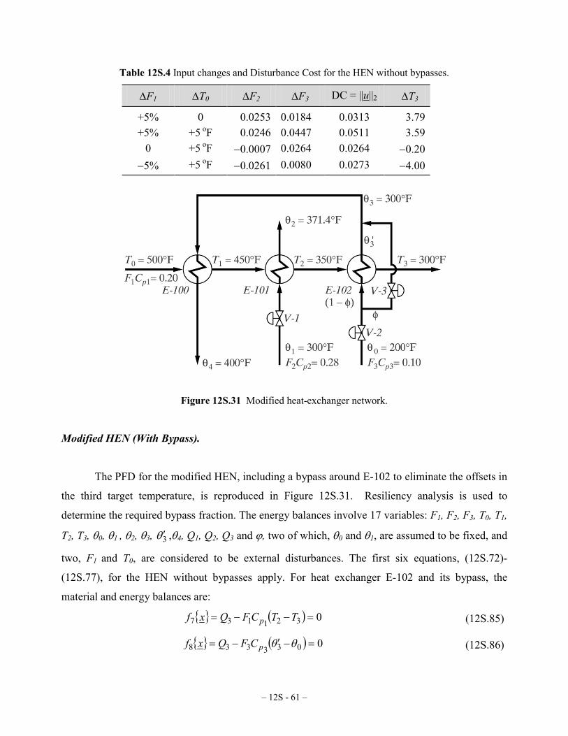
– 12S - 61 –
Table 12S.4 Input changes and Disturbance Cost for the HEN without bypasses.
∆F1 ∆T0 ∆F2 ∆F3 DC = ||u||2 ∆T3
+5% 0 0.0253 0.0184 0.0313 3.79 +5% +5 oF 0.0246 0.0447 0.0511 3.59
0 +5 oF −0.0007 0.0264 0.0264 −0.20 −5% +5 oF −0.0261 0.0080 0.0273 −4.00
Figure 12S.31 Modified heat-exchanger network.
Modified HEN (With Bypass).
The PFD for the modified HEN, including a bypass around E-102 to eliminate the offsets in
the third target temperature, is reproduced in Figure 12S.31. Resiliency analysis is used to
determine the required bypass fraction. The energy balances involve 17 variables: F1, F2, F3, T0, T1,
T2, T3, θ0, θ1 , θ2, θ3, 3θ ′ ,θ4, Q1, Q2, Q3 and ϕ, two of which, θ0 and θ1, are assumed to be fixed, and
two, F1 and T0, are considered to be external disturbances. The first six equations, (12S.72)-
(12S.77), for the HEN without bypasses apply. For heat exchanger E-102 and its bypass, the
material and energy balances are:
( ) 0321137 =−−= TTCFQxf p (12S.85)
( ) 0033338 =−′−= θθpCFQxf (12S.86)
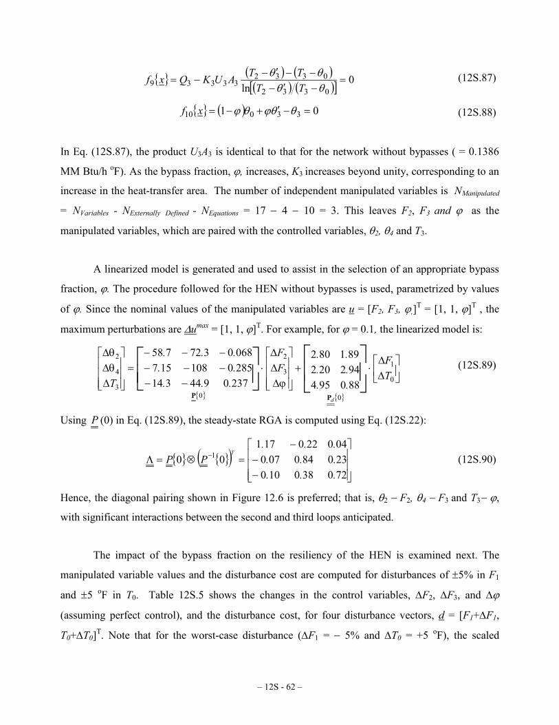
– 12S - 62 –
( ) ( )( ) ( )[ ] 0
ln 0332
033233339 =
−′−−−′−
−=θθθθ
TTTTAUKQxf (12S.87)
( ) 01 33010 =−′+−= θθϕθϕxf (12S.88)
In Eq. (12S.87), the product U3A3 is identical to that for the network without bypasses ( = 0.1386
MM Btu/h oF). As the bypass fraction, ϕ, increases, K3 increases beyond unity, corresponding to an
increase in the heat-transfer area. The number of independent manipulated variables is NManipulated
= NVariables - NExternally Defined - NEquations = 17 − 4 − 10 = 3. This leaves F2, F3 and ϕ as the
manipulated variables, which are paired with the controlled variables, θ2, θ4 and T3.
A linearized model is generated and used to assist in the selection of an appropriate bypass
fraction, ϕ. The procedure followed for the HEN without bypasses is used, parametrized by values
of ϕ. Since the nominal values of the manipulated variables are u = [F2, F3, ϕ,]T = [1, 1, ϕ]T , the
maximum perturbations are ∆umax = [1, 1, ϕ]T. For example, for ϕ = 0.1, the linearized model is:
∆∆
⋅+
ϕ∆∆∆
⋅−−
−−−−−−
=
∆θ∆θ∆
0
1
0
3
2
03
4
2
880954942202891802
237094431428501081570680372758
TF
..
..
..FF
........
TdPP
(12S.89)
Using P (0) in Eq. (12S.89), the steady-state RGA is computed using Eq. (12S.22):
( )
−−
−=⊗=Λ −
720380100230840070040220171
00 1
...
...
...PP
T (12S.90)
Hence, the diagonal pairing shown in Figure 12.6 is preferred; that is, θ2 − F2, θ4 − F3 and T3− ϕ,
with significant interactions between the second and third loops anticipated.
The impact of the bypass fraction on the resiliency of the HEN is examined next. The
manipulated variable values and the disturbance cost are computed for disturbances of ±5% in F1
and ±5 oF in T0. Table 12S.5 shows the changes in the control variables, ∆F2, ∆F3, and ∆ϕ
(assuming perfect control), and the disturbance cost, for four disturbance vectors, d = [F1+∆F1,
T0+∆T0]T. Note that for the worst-case disturbance (∆F1 = − 5% and ∆T0 = +5 oF), the scaled
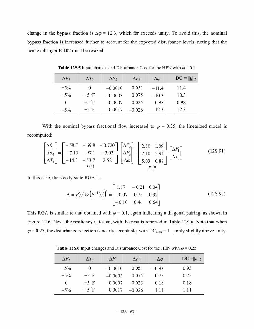
– 12S - 63 –
change in the bypass fraction is ∆ϕ = 12.3, which far exceeds unity. To avoid this, the nominal
bypass fraction is increased further to account for the expected disturbance levels, noting that the
heat exchanger E-102 must be resized.
Table 12S.5 Input changes and Disturbance Cost for the HEN with ϕ = 0.1.
∆F1 ∆T0 ∆F2 ∆F3 ∆ϕ DC = ||u||2
+5% 0 −0.0010 0.051 −11.4 11.4 +5% +5 oF −0.0003 0.075 −10.3 10.3
0 +5 oF 0.0007 0.025 0.98 0.98 −5% +5 oF 0.0017 −0.026 12.3 12.3
With the nominal bypass fractional flow increased to ϕ = 0.25, the linearized model is
recomputed:
( ) ( )
∆∆
⋅+
∆∆∆
⋅−−
−−−−−−
=
∆∆∆
0
1
0
3
2
03
4
2
880035942102891802
5227533140231971577200869758
TF
..
..
..FF
.........
TdPP
ϕθθ
(12S.91)
In this case, the steady-state RGA is:
( ) ( )( )
−−
−=⊗=Λ −
640460100320750070040210171
00 1
...
...
...PP
T
(12S.92)
This RGA is similar to that obtained with ϕ = 0.1, again indicating a diagonal pairing, as shown in
Figure 12.6. Next, the resiliency is tested, with the results reported in Table 12S.6. Note that when
ϕ = 0.25, the disturbance rejection is nearly acceptable, with DCmax = 1.1, only slightly above unity.
Table 12S.6 Input changes and Disturbance Cost for the HEN with ϕ = 0.25.
∆F1 ∆T0 ∆F2 ∆F3 ∆ϕ DC =||u||2
+5% 0 −0.0010 0.051 −0.93 0.93 +5% +5 oF −0.0003 0.075 0.75 0.75
0 +5 oF 0.0007 0.025 0.18 0.18 −5% +5 oF 0.0017 −0.026 1.11 1.11

– 12S - 64 –
Clearly, the resiliency of the HEN increases with the nominal bypass fraction, but at the
cost of increased heat-transfer area. Table 12S.7 shows the trade-off between resiliency and heat-
transfer area. Note that while only 12% additional heat-exchange area is required for ϕ = 0.1, the
resiliency is inadequate. In contrast, when ϕ = 0.30, the resiliency is satisfactory (with DC
significantly lower than unity), but the heat-transfer area is doubled. A good compromise is to
select ϕ = 0.25, which approximates the desired resiliency, while requiring only 55% more heat-
exchange area.
Table 12S.7 Trade-off between the heat-exchanger area and bypass fraction.
ϕ DC = ||u||2 K3
0.10 12.3 1.12 0.15 4.63 1.21 0.20 2.16 1.33 0.25 1.11 1.55 0.30 0.58 2.05
The C&R analysis in the steady state predicts the superior performance of the modified
HEN, which allows all three target temperatures to be controlled at their setpoints in the face of
disturbances in the feed flow rate and temperature of the hot stream. More specifically, the steady-
state RGA indicates that a decentralized control system can be configured for the modified HEN in
which θ2 − F2, θ4 − F3 and T3− ϕ are paired, and in which the first loop is almost perfectly
decoupled, with moderate coupling between the other two loops. Finally, aided by DC analysis, the
nominal bypass fraction is selected to be 0.25, providing the best trade-off between increased plant
costs and adequate resiliency.
Given the design decision to use ϕ = 0.25, based upon the steady-state C&R analysis,
verification is performed by dynamic simulations with ASPEN HYSYS. The hot stream of n-octane at
2,350 lbmol/h is cooled from 500 to 300 oF using n-decane as the coolant, with F2 = 3,070 lbmol/h
and F3 = 1,200 lbmol/h. Note that these species and flow rates are chosen to match the heat-
capacity flow rates defined by McAvoy (1983), with F1 slightly increased to avoid temperature
crossovers in the heat exchangers due to temperature variations in the heat capacities. Additional
details of the ASPEN HYSYS simulation are:
– 12S - 65 –
(a) The tubes and shells for the heat exchangers provide 2 min residence times.
(b) The feed pressures of all three streams are set at 250 psi, with nominal pressure drops of
5 psi defined for the tubes, shells and for the bypass valve, V-3. Subsequently, these
pressure drops are computed based on the equipment and valve sizing and the pressure-
flow relationships.
(c) The bypass valve V-3 is sized carefully, ensuring that the nominal bypass fraction is
0.25, with the nominal valve position being 50% open (selecting a linear characteristic
curve).
(d) IMC-PI tuning parameters are presented in Table 12S.8.
Table 12S.8 IMC-PI tuning parameters for the alternative HENs.
HEN without bypass (Figures 12S.30 and 12.5)
Loop PV Range,oF Kc τI, min Action θ2 − F2 300-500 2 1.5 Direct θ4 − F3 300-500 1.5 2.5 Direct
HEN with bypass (Figures 12S.31 and 12.6)
Loop PV Range,oF Kc τI, min Action θ2 − F2 300-500 2 1 Direct θ4 − F3 300-500 1 2 Direct T3− ϕ 300-500 1 1 Reverse
The regulatory responses of the two configurations are discussed next. Figure 12S.32 shows
that, as predicted by the DC analysis, even the worst-case disturbance has little effect on the two
controlled variables, whose control loops are decoupled, as indicated by the RGA analysis.
Moreover, the uncontrolled output, T3, exhibits offsets of about ±4.5 oF, which compare well with
the value of ±4 oF predicted by the linear DC analysis. In comparison, Figure 12S.31 shows that,
for the HEN with bypass, the response also corroborates the results of the linear DC analysis. Most
importantly, the design with ϕ = 0.25 rejects the worst-case disturbance with no saturation,
indicating that the DC analysis is slightly conservative. In addition, the first control loop (θ2 − F2) is
perfectly decoupled, with slight interactions seen in the other two loops, again as predicted by the
static RGA analysis. For more details, the reader is referred to the section covering dynamic
simulation using ASPEN HYSYS on the multimedia CD-ROM that accompanies this text, where
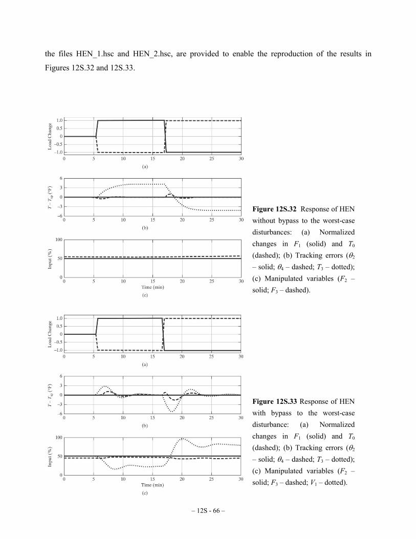
– 12S - 66 –
the files HEN_1.hsc and HEN_2.hsc, are provided to enable the reproduction of the results in
Figures 12S.32 and 12S.33.
Figure 12S.32 Response of HEN without bypass to the worst-case disturbances: (a) Normalized changes in F1 (solid) and T0 (dashed); (b) Tracking errors (θ2 – solid; θ4 – dashed; T3 – dotted); (c) Manipulated variables (F2 – solid; F3 – dashed).
Figure 12S.33 Response of HEN with bypass to the worst-case disturbance: (a) Normalized changes in F1 (solid) and T0 (dashed); (b) Tracking errors (θ2 – solid; θ4 – dashed; T3 – dotted); (c) Manipulated variables (F2 – solid; F3 – dashed; V1 – dotted).

– 12S - 67 –
While steady-state C&R analysis often provides a good assessment of the controllability
and resiliency, dynamic analysis should be considered when the steady-state analysis is
inconclusive. The latter methods are discussed by Wolff et al. (1991) and Mathisen et al. (1993).
Case Study 12S.3 Interaction of Design and Control in the MCB Separation Process
Denn and Lavie (1982) show that recycles increase the process response time and static
gain. Furthermore, when the recycle loop contains a time delay, resonant peaks comparable in
magnitude to the steady-state gain may result. Since these phenomena are potentially destabilizing,
control systems for recycle processes should be designed carefully. In this regard, control systems
for recycle processes are designed using the nine-step design procedure of Luyben and coworkers
(1999), presented in Section 12.3, with particular emphasis on the need to impose flow control on
each recycle stream.
Figure 12S.34 Flowsheet for the MCB separation process.
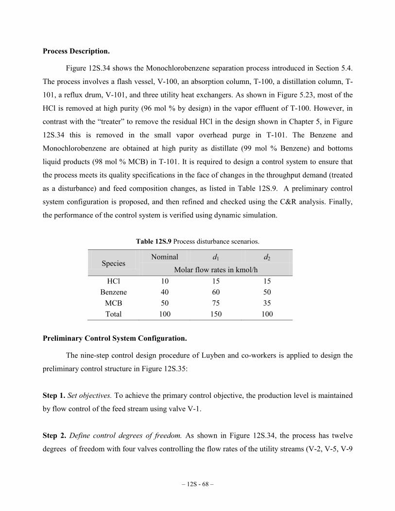
– 12S - 68 –
Process Description.
Figure 12S.34 shows the Monochlorobenzene separation process introduced in Section 5.4.
The process involves a flash vessel, V-100, an absorption column, T-100, a distillation column, T-
101, a reflux drum, V-101, and three utility heat exchangers. As shown in Figure 5.23, most of the
HCl is removed at high purity (96 mol % by design) in the vapor effluent of T-100. However, in
contrast with the “treater” to remove the residual HCl in the design shown in Chapter 5, in Figure
12S.34 this is removed in the small vapor overhead purge in T-101. The Benzene and
Monochlorobenzene are obtained at high purity as distillate (99 mol % Benzene) and bottoms
liquid products (98 mol % MCB) in T-101. It is required to design a control system to ensure that
the process meets its quality specifications in the face of changes in the throughput demand (treated
as a disturbance) and feed composition changes, as listed in Table 12S.9. A preliminary control
system configuration is proposed, and then refined and checked using the C&R analysis. Finally,
the performance of the control system is verified using dynamic simulation.
Table 12S.9 Process disturbance scenarios.
Species Nominal d1 d2
Molar flow rates in kmol/h HCl 10 15 15
Benzene 40 60 50 MCB 50 75 35 Total 100 150 100
Preliminary Control System Configuration.
The nine-step control design procedure of Luyben and co-workers is applied to design the
preliminary control structure in Figure 12S.35:
Step 1. Set objectives. To achieve the primary control objective, the production level is maintained
by flow control of the feed stream using valve V-1.
Step 2. Define control degrees of freedom. As shown in Figure 12S.34, the process has twelve
degrees of freedom with four valves controlling the flow rates of the utility streams (V-2, V-5, V-9
– 12S - 69 –
and V-10), one controlling the feed flow rate (V-1), three controlling product stream flow rates (V-
6, V-8 and V-11), and the four remaining valves controlling internal process flow rates. Having
chosen constant feed flow in Step 1, the feed valve (V-1) is reserved for independent flow control.
Step 3. Establish energy management system. The steam valve, V-2 is used to control the flash
feed temperature. Furthermore, the temperature of the recycle and bottoms product streams is
contolled by adjusting the coolant valve, V-10.
Step 4. Set the production rate. As stated previously, the feed valve, V-1, is assigned to a flow
controller, whose setpoint regulates the production rate.
Step 5. Control product quality, and meet safety, environmental and operational constraints. The
pressure in V-100 is controlled by adjusting its vapor stream using valve, V-3. Pressure regulation
in the T-101 is carried out by adjusting V-5, the coolant valve to the condenser E-101. Since both
of the products from T-101 are required to meet specifications, the LV configuration is
implemented, noting that the reflux ratio in the column is less than five. Thus, the reflux valve, V-7,
is adjusted to control the distillate composition, and the reboiler steam valve, V-9, is used to
regulate the bottoms composition.
Step 6. Fix recycle flow rates and vapor and liquid inventories. The obvious choice for recycle
flow control is valve V-12. The liquid inventories in the flash drum, the reflux drum and the
column sump, are regulated using the valves V-4, V-8 and V-11, respectively. Note that the purge
stream that removes the residual HCl from the column overheads is less that 1% of the feed by
design. Thus, the valve V-6 is designed to fixed at 50% open and left uncontrolled. Regulations of
the vapor inventories in both V-100 and T-101 have been addressed, by installing pressure
controllers.
Steps 7 and 8. Check component balances and control individual process units. The HCl in the
feed is removed from the process, mostly in the T-100 overhead stream, with small traces removed
in the column purge stream. The benzene and MCB fed to the process are mostly removed in the
distillate and bottoms streams from T-101, respectively, with small traces removed with the HCl
product and in the purge.
Step 9. Optimize economics and improve dynamic controllability. It is noted that all of the control
valves have been assigned, but the HCl product quality is still uncontrolled. To correct this, a
– 12S - 70 –
cascade controller is installed to regulate the HCl product stream composition, which adjusts the set
point of either (a) the recycle flow controller, FC-2, or (b) the recycle temperature controller, TC-2.
Figure 12S.35 shows the first alternative, which manipulates the liquid feed rate to the absorber to
control the mass transfer of the organic species from the vapor stream. Clearly, quantitative
methods are required to enable the most appropriate configuration to be selected, as will be shown
next.
Figure 12S.35 Control system for the MCB separation process.
Control System Refinement using C&R Analysis.
Controllability and resiliency analysis has two roles in the improvement of the control
system in Figure 12S.35: (1) The RGA aids in defining the appropriate pairing between the
controlled outputs and manipulated variables where interaction is anticipated; (2) The DC assists in
checking that the operating ranges of key manipulated variables is sufficient to ensure adequate

– 12S - 71 –
disturbance rejection. To provide data for these two analytical methods, a dynamic simulation of
the MCB separation process is developed using ASPEN HYSYS.
The equipment items are sized as follows:
(a) The flash vessel, V-100, condenser, V-101 and reboiler, E-102, are installed assuming at
least 10 min liquid residence time, computed using the steady-state liquid feed rate as a
basis. Thus, for example, since the liquid feed to V-100 is nominally 137 ft3/hr, the
required vessel volume is 2×10×137/60 = 45.7 ft3, which is rounded up to 50 ft3. Similar
calculations give volumes of 120 ft3 for V-101 and 240 ft3
for E-102.
(b) The absorption column, T-100, is a 10-stage packed bed with a diameter of 1.5 ft.
(c) The distillation column, T-101, has 10 valve-trays with a diameter of 2.5 ft.
(d) The two heat exchangers are approximated as heat-requirement units, which assume that
the control variable is the heat transfer duty. Thus, E-100 is installed as a heater, with
volume of 20 ft3 and E-103 as a cooler, with a volume of 50 ft3. More detailed modeling
is possible by using heat exchangers, allowing the manipulation of steam and cooling
water flows. Pressure drops in these heat exchangers are defined by assigning a
pressure-flow relationship, established automatically by ASPEN HYSYS on the basis of
nominal flow rates.
(e) A number of valves are installed to enable flow and pressure regulation of the process.
Each valve is set to be 50% open, sized on the basis of nominal flow rates, and then
assigned to follow a pressure-flow relationship. When a valve is selected to provide
control, it is assigned to a controller, which manipulates the percentage valve opening.
One valve that is maintained at 50% open is V-6, which is intended to purge the residual
light gases in the feed to T-101.
Several of the control loops in Figure 12S.35 are required to ensure inventory control,
namely, all three level control loops and the two pressure control loops. Note that the pressure in V-
100 is assumed constant and the loop PC-1 is not simulated explicitly in the ASPEN HYSYS
simulation. In contrast, as pointed out repeatedly in the literature, pressure control in the column is
crucial to stabilize the internal flows in the column. Finally, the feed flow rate and temperature
controllers are clearly decoupled from the rest of the process, and therefore need not be included in

– 12S - 72 –
the C&R analysis. Thus, the interactions that need to be analyzed are the effects of the four valves:
V-7, V-9, V-10 and V-12 (or more precisely, the setpoint to FC-1), on four controlled variables:
xD,2, xB,3, xA,1 (the mole fractions of the benzene in the distillate, MCB in the bottoms and HCl in
the absorber overhead stream, respectively) and TR, the recycle temperature. Note that to improve
dynamic performance, the temperature of tray 4 is controlled instead of the distillate benzene
composition.
The interaction analysis is performed using the steady-state RGA. To generate information
to compute RGA, the loops under test in the simulated process are placed in “manual” mode, and
the process is simulated to “line-out” the outputs at open-loop steady-state values. Then, distinct
step changes in the four valve positions are imposed, and the new steady-state values of the outputs
recorded. Note that for consistency, the step direction is chosen such that its effect on AC-1 is in
the same direction. The results of these simulations are recorded in Table 12S.10. Thus, for
example, a 0.5% increase in the position of the reflux valve (V-7) leads to a decrease of 4.5 oF in
temperature in tray 4.
Table 12S.10 Simulation results for RGA calculations.
R (V-7) xD,2 (AC-1) xB,3 (AC-2) xA,1 (AC-3) TR(TC-2) Range 0-100 % 100-300 oF 0.5-1.0 0.5-1.0 50-250 oF Before 43.0 % 226.3 oF 0.9857 0.9596 121.2 oF After 43.5 % 221.8 oF 0.9638 0.9590 117.9 oF
Change +0.5% –4.5 oF –0.0219 –0.0006 –3.3 oF QR (V-9) xD,2 (AC-1) xB,3 (AC-2) xA,1 (AC-3) TR(TC-2)
Before 45.4 % 226.3 oF 0.9857 0.9596 121.2 oF After 44.9 % 221.5 oF 0.9576 0.9589 116.8 oF
Change –0.5% –4.8 oF –0.0281 –0.0007 –4.4 oF FR (FC-2) xD,2 (AC-1) xB,3 (AC-2) xA,1 (AC-3) TR(TC-2)
Before 45.0 % 226.3 oF 0.9857 0.9596 121.2 oF After 45.5 % 224.9 oF 0.9817 0.9582 122.1 oF
Change +0.5% –1.4 oF –0.0040 –0.0014 +1.1 oF QC (V-10) xD,2 (AC-1) xB,3 (AC-2) xA,1 (AC-3) TR(TC-2)
Before 76.0 % 226.3 oF 0.9857 0.9596 121.2 oF After 76.5 % 224.3 oF 0.9803 0.9605 119.0 oF
Change +0.5% –2.0 oF –0.0054 +0.0011 –2.2 oF
– 12S - 73 –
Dimensionless static gains are computed, accounting for the full range of each variable.
Thus, for example, the gain that relates variations of xD,2 to changes in R is:
5410050200540 2
11 ...
Rx
p ,D −=−
=∆
∆= (12S.93)
In the same way, the other 15 static gains are computed, given the overall steady-state transfer-
function matrix relationship:
−−−−
−−−−−−
=
C
R
R
R
,A
,B
,D
QFQR
...............
Txxx
221014043034405602802401626012118.76002401804504
1
3
2
(12S.94)
The RGA is computed from this linear model:
−−−−
−−−−
=Λ
019989859869112115811715
639447284100731351711815
........
.......
(12S.95)
The large RGA elements are indicative of significant sensitivity to model uncertainty, often related
to process nonlinearities. While the RGA indicates that the pairings: xD,2 – R, xB,3 – QR, xA,1 – QC,
and TR – FR, provide stable response, the large RGA elements are indicative of large interactions in
the process.
The above results, however, suggest a simpler control structure, in which FR is maintained
constant, and QC is adjusted to control xA,1, giving the steady-state transfer-function matrix
relationship:
−−−−−
=
C
R
,A
,B
,D
QQR
........
xxx
4402802401622118.76002804504
1
3
2 (12S.96)
In this case, the RGA is:
−−
−=Λ
83904990660005302963451070794696
...
...
... (12S.97)
– 12S - 74 –
This suggests performance superior to that obtained with the original confirmation using the
diagonal pairings: xD,2 – R, xB,3 – QR, and xA,1 – QC , leading to the modified control system shown
in Figure 12S.36. Note in particular, that the third loop is almost decoupled, with strong
interactions in the two distillation-column loops. The large RGA elements associated with the LV
configuration are significantly larger than those expected in a column operating independently
(compared with those computed for the SC configuration in Figure 12S.16), due to the additional
positive feedback contributed by the material recycle.
Figure 12S.36 Improved control system for the MCB separation process.
Next, the DC is computed for typical process load changes and disturbances, presented in
Table 12S.9. Two scenarios are considered: d1, a 50% increase in throughput, and d2, a composition
disturbance in which all three compositions are changed. Table 12S.11 shows the open-loop effect
each disturbance on the four outputs, indicating that the second disturbance has the greatest effect
on the top composition in T-101. The effect of the two disturbances on the three outputs controlled
by the control system in Figure 12S.36, expressed in scaled perturbation variable form, are:
– 12S - 75 –
For disturbance 1:
−−−
=⋅479601420001950
01...
dPd (12S.98)
For disturbance 2:
=⋅
033600398018350
02...
dPd (12S.99)
Note that the scaled perturbation variables are computed by dividing the changes on the output
variables in Table 12S.11 by their full-scale ranges. This allows the steady-state DC to be
computed directly:
[ ]
−−
=
−−−
−−−−−
=
−=
−
−
910307941025591
479601420001950
4402802401622118.76002804504
000 :1 edisturbancFor 1
11
...
.
.
.
........
dPPDC d
(12S.100)
[ ]
−=
−−−−−
=
−=
−
−
053302208029990
033600398018350
4402802401622118.76002804504
000 :2 edisturbancFor 1
11
...
.
.
.
........
dPPDC d
(12S.101)
The linear analysis suggests that the effect of the first disturbance cannot be rejected completely,
because it causes the first control variable, R, to saturate (the magnitude of the DC for this variable
is greater than unity). In contrast, the linear DC analysis predicts that the second disturbance is
rejected relatively easily. Table 12S.11 Data for DC calculations.
(a) Disturbance 1: Increased throughput by 50 %
xD,2 (AC-1) xB,3 (AC-2) xA,1 (AC-3) TR(TC-2) Range 100-300 oF 0.5-1.0 0.5-1.0 50-250 oF Before 226.3 oF 0.9857 0.9596 121.2 oF After 222.4 oF 0.9148 0.7200 141.1 oF
Change –3.9 oF –0.0709 –0.2396 +39.9 oF
(b) Disturbance 2: Composition change.
xD,2 (AC-1) xB,3 (AC-2) xA,1 (AC-3) TR(TC-2) Before 226.3 oF 0.9857 0.9596 121.2 oF After 263.0 oF 0.9976 0.9764 90.8 oF
Change 36.7 oF 0.0199 0.0168 –30.4 oF

– 12S - 76 –
Dynamic simulation using ASPEN HYSYS is used to verify the predictions of the linear
C&R analysis. The control loops shown in Figure 12S.36 are all PI controllers, with tuning
parameters tuned using the IMP-PI rules, given in Table 12S.12. Note that the level controllers are
loosely tuned, as in Case Study 12S.1. In contrast, the distillation column pressure controller, PC-2,
is tuned to ensure tight control of this key variable. The gains on the three composition controllers,
AC-1, AC-2 and AC-3, are tuned to ensure that the strong interaction between them does not lead
to loss of stability, while imparting acceptable regulatory performance.
Figure 12S.37 Response of the MCB separation
process to a 50% increase in throughput (d1):
(a) molar feed rates in kmol/hr – solid = MCB,
dashed = benzene, dotted = HCl; (b) changes in
product purities in % – solid = MCB, dashed =
benzene, dotted = HCl; (c) manipulated variables
– solid = V-9 (QR), dashed = V-7 (R), dotted =
V-10 (QC); (d) product flow rates in kmol/h– solid
= MCB, dashed = benzene, dotted = HCl.

– 12S - 77 –
Figure 12S.38 Response of the MCB separation
process to composition change disturbance (d2).
(a) Molar feed rates in kmol/hr, (b) changes in
product purities in %, (c) manipulated variables,
(d) product flow rates in kmol/h. Variables as in
Figure 12S.37.
The simulations shown in Figures 12S.37 and 12S.38 show that:
a) The 3×3 control system, paired as suggested by the RGA, provides stable performance
for both disturbances.
b) Both of the disturbances are step changes in the molar feed rates in the three species.
Note that the control system manipulates the draw rates needed while ensuring that the
product compositions stay on specification, by the action of the level controllers (see
Figures 12S.37d and 12S.38d).

– 12S - 78 –
c) The effects of both of the disturbances on the purities of the three products are rejected
successfully, despite the prediction of the linear DC analysis (see Figures 12S.37b and
12S.38b). The control action perturbations required to reject the first disturbance are
greater than for the second one, which is qualitatively in agreement with the DC
analysis (see Figures 12S.37c and 12S.38c).
Table 12S.12 IMC-PI tuning parameters for the MCB Separation Process (See Figure 12S.36).
Loop PV Range Set point Kc τi Action TC-1 150-350 oF 270 oF 3 2 min Reverse FC-2 0-200 lbmol/h 90 lbmol/h 1.4 0.5 min Reverse AC-1 200-300 oF 226.3 oF 5 25 min Direct AC-2 0.50-1.00 MCB 0.98 MCB 12 10 min Reverse AC-3 0.50-1.00 HCl 0.97 HCl 12 20 min Reverse PC-2 15-40 psia 26 psia 3 0.5 min Direct LC-1 0-100% 50% 2 30 min Direct LC-2 0-100% 50% 2 30 min Direct LC-3 0-100% 50% 2 30 min Direct
This case study has shown the advantages of employing C&R analysis to assist in the
design of a plant-wide control system using the procedure of Luyben and co-workers. The control
configuration pairing is determined using the steady-state RGA. The disturbance rejection afforded
by the process is predicted incorrectly by the linear DC analysis. This indicates that non-linear
approaches should be used in general. Nonlinear controllability and resiliency analysis is an area of
active research (e.g., Seferlis and Grievink, 1999; Solovyev and Lewin, 2001).
12S.6 MATLAB FOR C&R ANALYSIS
MATLAB and SIMULINK are invaluable tools for the frequency- and time-domain
calculations required for C&R analysis. In this section, several examples are carried out using
MATLAB, it being assumed that the reader is familiar with the MATLAB syntax. The reader is
referred to the multimedia CD-ROM that accompanies this text for sources of these and other
useful MATLAB functions and scripts for C&R analysis. In particular, the interactive C&R
– 12S - 79 –
Tutorial CRGUI can be used to test three example linear processes for controllability and resiliency
and simulate their closed-loop response under single-loop PI control.
Example 12S.11 Computing the Dynamic RGA
For the system given in Example 12S.3, the MATLAB script that generates the dynamic RGA in
Figure 12S.5 is:
% Example 12S.3 % This script file computes the dynamic RGA for Example 12S.3 % Define a vector of frequency values on a log scale wmin=-3;wmax=1;nw=30*fix(wmax-wmin); w=logspace(wmin,wmax,nw); s=i*w; % Data for process model kp=[2.5 5;1 -4]; %process gain matrix tp1=[15 4;3 20]; %process time constant tp2=[2 0;0 0]; %process time constant thp=[5 0;0 5]; %process delay % Compute the frequency response for each element of Pij p11=kp(1,1)./(tp1(1,1)*s+1)./(tp2(1,1)*s+1).*exp(-thp(1,1)*s); p12=kp(1,2)./(tp1(1,2)*s+1)./(tp2(1,1)*s+1).*exp(-thp(1,2)*s); p21=kp(2,1)./(tp1(2,1)*s+1)./(tp2(1,1)*s+1).*exp(-thp(2,1)*s); p22=kp(2,2)./(tp1(2,2)*s+1)./(tp2(1,1)*s+1).*exp(-thp(2,2)*s); % Compute lambda(1,1) and lambda(1,2) as functions of frequency. l11=p11.*p22./(p11.*p22-p12.*p21); lam11=sign(real(l11(1))).*abs(l11); l12=-p12.*p21./(p11.*p22-p12.*p21); lam12=sign(real(l12(1))).*abs(l12); %Plot the results figure semilogx(w,lam11,'-k',w,lam12,':k','LineWidth',2) xlabel('\omega [rad/min]','FontName','Times','FontSize',14) ylabel('DRGA','FontName','Times','FontSize',14)

– 12S - 80 –
As discussed in Example 12S.3, the steady-state RGA suggests diagonal pairings. However,
the dynamic RGA implies that these pairings are unstable for frequencies higher than about 0.5
rad/min. Thus, anti-diagonal pairings should be used.
Example 12S.12 Computing Disturbance Cost Maps
Consider the component parts in the LSF configuration represented by Eqs. (12S.56) and (12S.57).
In this example, the elements of the transfer function matrices are entered into MATLAB and used
to compute the DC contour maps for this configuration. P j P jdω ω and are computed for each
frequency, and used to compute DC for all of the disturbance directions. By looping over all
frequencies, the entire DC map is calculated, and repeated for each manipulated variable separately.
Note that, as mentioned in Example 12S.7, the inputs are nominally at 50% of the full range. Here,
the nominal inputs are taken as LH = LL = 11 kmol/min, QRH = 0.222×10⁶ kcal/min, and the
maximum disturbance magnitudes are taken as F=18 kmol/min and xF = 0.2 (±20% of the full
range).
% LFS: This script computes P(s) and Pd(s) for the LSF configuration, given the % transfer-function matrices for the two component parts. It then uses the % matrices to compute DC contours % Definition of frequency and direction vectors. n=41; i=sqrt(-1); wmin=-3; wmax=0; dw=(wmax-wmin)/(n-1); tmin=0; tmax=180; dt=(tmax-tmin)/(n-1); w=logspace(wmin,wmax,n); % Frequency vector [rad/min] ome=wmin:dw:wmax; % Frequency vector in log scale. phi=tmin:dt:tmax; % Direction vector [degrees] a=pi*phi/180; % Direction vector [radians] s=w*i; % Vector complex s tt = exp(i*a); % Computing the direction in radian coordinates dd(1:n,1:2) = [real(tt'),imag(-tt')]; % tt in cartesian coordinates z=zeros(1:n,1:n); % matrix for storing computed DC values. % Gains and delay times for the high pressure column: KH=[0.017 -1.109 0.001 0.090; 0.011 -1.859 0.006 1.296; -0.33 59.0 -0.2 -41.05; 0.916 -123.7 1.127 -0.02; 4.0e-5 -0.994 0.001 0.003]; DH=[0.0 0.0 0.0 6.4; 1.3 0.0 0.1 0.1; 1.3 0.0 0.1 0.1;1.3 0.0 0.1 0.1;1.3 0.0 0.1 0.1]; % Gains and delay times for the low pressure column: KL=[ 0.792 -0.029 0.007 2.161 0.012; 0.790 -0.051 0.003 3.291 0.038];

– 12S - 81 –
% Note: The coefficients in the fourth column have been multiplied by -1 % since QRL = - QCH DL=[ 0.1 0.1 0.1 0.0 1.4;8.5 0.0 0.0 0.0 0.0];
for ku=1:3 % Looping over all manipulated variables (m=3) for k=1:n % Looping over all frequencies. % Computing the frequency response of each component part submatrix [see % Eqns. (12S.56) and (12S.57)]. ph=KH.*exp(-DH*s(k))./(13*s(k)+1); pl=KL.*exp(-DL*s(k))./(17*s(k)+1); % Computing P(s) and Pd(s) at the current frequency [See Eqns. (12S.60) % and (12S.61)] P=[ph(:,1:4) 0 ; pl(1,1:2)*ph(2:5,1:2) pl(:,:5)]; Pd=[ph(1,3:4) ; pl(:,1:4)*ph(2:5,3:4)]; % Scaling: P(:,1)=P(:,1)*11;P(:,2)=P(:,2)*0.222;P(:,3)=P(:,3)*11; Pd(:,1)=Pd(:,1)*18;Pd(:,2)=Pd(:,2)*0.2; u2 = inv(P)*Pd*dd'; % Computing DC for i_dir = 1:n % Looping over d direction 0 → 180 z(i_dir,k) = norm(u2(ku,i_dir)); end end % End of frequency loop. v = [0.1 0.2 0.3 0.4 0.5 0.6 0.7 0.8 0.9 1.0]; figure cs=contour(ome,phi,z); clabel(cs) title(['Disturbance Cost for Input ',num2str(ku)]); xlabel('log(w)'); ylabel('Direction [deg]'); end % End of manipulated-variable loop
This script generates the DC contour maps in Figure 12S.39 for each manipulated variable
separately. Note that there is no bandwidth limitation to perfect disturbance rejection in any of the
control variables.

– 12S - 82 –
Figure 12S.39 DC contour maps for the LSF
configuration to dehydrate methanol: (a) LH;
(b) QRH; (c) LL. The bounds on the disturbances
are ±20% from their nominal values. The DC
contour maps for each manipulated variable are
computed separately, with bold solid lines
indicating DC = 1. See Figure 12S.17 for the DC
contour maps for the SC, FS and LSR
configurations.
12S.7 SUMMARY
In this chapter, the methods for short-cut C&R analysis, using the results of steady-state
simulations, have been described. The methods require the use of software for the solution of
material and energy balances in process flowsheets (e.g., ASPEN PLUS, HYSYS.Plant) and for
controllability and resiliency analysis (i.e., MATLAB). The reader is now prepared to tackle small-
to medium-scale problems, and in particular, should be able to

– 12S - 83 –
1. Generate a linear model of a chemical process in one of its standard forms, using
either the equations expressed in a MATLAB function, or the solution of the
material and energy balances computed by a process simulator.
2. Compute the frequency-dependent process transfer functions using MATLAB, given
a linear model in one of its standard forms.
3. Generate the C&R measures of relative-gain array (RGA) and disturbance cost
(DC), given the process transfer functions, using MATLAB.
4. Select the appropriate pairings for a decentralized control system for the process
using the static and dynamic RGAs and appropriate resiliency measures.
5. Perform C&R analysis to select between alternative process configurations, given
the results of process simulations.
Several examples have been selected to show how the methods are used to screen
alternative flowsheets in stage 2 of the design process (Table 12.1). In the first example (Section
21.3), dynamic C&R analysis enables the most resilient heat-integrated distillation configuration to
be selected. In Case Study 12S.1, two designs for an exothermic reactor, involving either one or
two CSTR(s) in series, show that while the latter is more economical (assuming steady-state
operation), the former is more resilient to disturbances. In Case Study 12S.2, a steady-state analysis
of two heat exchanger network configurations leads to the conclusion that while a design equipped
with bypasses may be subject to significant constraints leading to poor resiliency, a design without
them may lead to poor dynamic performance. Here, dynamic C&R analysis is crucial. Finally, Case
Study 12S.3, involves a recycle processes and shows the benefits of C&R analysis in the detailed
design stage (Stage 3 in Table 12.1).
REFERENCES
Bequette, B.W., Process Dynamics: Modeling, Analysis, and Simulation, Prentice Hall, Englewood
Cliffs, NJ, (1998).
Bristol, E. H., On a New Measure of Interactions for Multivariable Process Control, IEEE Trans.
Auto. Control, AC-11, 133-134 (1966).
Chiang, T., and W. L. Luyben, Comparison of the Dynamic Performances of Three Heat-integrated
Distillation Configurations, Ind. Eng. Chem. Res., 27, 99-104 (1988).

– 12S - 84 –
Denn, M. M., and R. Lavie, Dynamics of Plants with Recycle, Chem. Eng. J., 24, 55-59 (1982).
Lewin, D. R., A Simple Tool for Disturbance Resiliency Diagnosis and Feedforward Control
Design, Comput. Chem. Eng., 20 (1), 13-25 (1996).
Lewin, D. R., and D. Bogle, Controllability Analysis of an Industrial Polymerization Reactor,
Comput. Chem. Eng., 20 (S), S871-S876 (1996).
Lewin, D. R., W. D. Seider, J. D. Seader, E. Dassau, J. Golbert, G. Zaiats, D. Schweitzer, D.
Goldberg, M. Fucci, and R. B. Nathanson, Using Process Simulators in the Chemical
Engineering Curriculum – A Multimedia Guide for the Core Curriculum, Version 2.0,
Multimedia CD-ROM, John Wiley, New York (2003).
Luyben, W.L., Process Modeling, Simulation and Control for Chemical Engineers, 2nd ed.,
McGraw-Hill, New York (1990).
Luyben, W. L., B. D. Tyreus, and M. L. Luyben, Plantwide Process Control, McGraw-Hill, New
York (1999).
Mathisen, K.W., S. Skogestad, and E. A. Wolff, Bypass Selection for Control of Heat Exchanger
Networks, Comput. Chem. Eng., 16 (S), S263-S272 (1993).
McAvoy, T.J. Interaction Analysis, Instrument Society of America, Research Triangle Park, NC
(1983).
Morari, M. Design of Resilient Processing Plants III, A General Framework for the Assessment of
Dynamic Resilience, Chem. Eng. Sci., 38, 1881-1891 (1983).
Morari, M., and E. Zafiriou, Robust Process Control, Prentice-Hall, Englewood Cliffs, NJ (1989).
Naot, I., and D. R. Lewin, Analysis of Process Dynamics in Recycle Systems Using Steady State
Flowsheeting Tools, Proc. 4th IFAC Symposium on Dynamics and Control of Chemical
Reactors, Distillation Columns and Batch Processes (DYCORD'95), Helsingor, Danish
Automation Society, Copenhagen (1995).
Ogunnaike, B. A., and W. H. Ray, Process Dynamics, Modeling and Control, Oxford Univ. Press,
New York (1994).
Perkins, J. D. The Interaction Between Process Design and Process Control, Proc. IFAC
Symposium on Dynamics and Control of Chemical Reactors and Distillation Columns
(DYCORD'89), 195-203 (1989).
Prett, D. M., and M. Morari, Shell Process Control Workshop, Butterworth, Stoneham, MA, 355-
360 (1986).

– 12S - 85 –
Rivera, D. E., S. Skogestad, and M. Morari, Internal Model Control. 4. PID Controller Design, Ind.
Eng. Chem. Res., 25, 252-265 (1986).
Rotstein, G. E. and D. R. Lewin, Simple PI and PID Tuning for Open Loop Unstable Systems, I. &
E. C. Res., 30, 1864-1869 (1991).
Russo L. P., and B. W. Bequette, Operability of Chemical Reactors: Multiplicity Behavior of a
Jacketed Styrene Polymerization Reactor, Chem. Eng. Sci., 53(1), 27-45 (1998)
Sandelin, P. M., K. E. Haggblom and K.V. Waller, Indirect Two-Point Control Through One-Point
Control of Distillation, in J.E. Rijnsdorp, J.F. MacGregor, B.D. Tyreus, and T. Takamatsu,
(eds.), Dynamics and Control of Chemical Reactors, Distillation Columns and Batch
Processes, IFAC Symposia Series 1990, No. 7, Pergamon Press, Oxford, 143-148 (1990).
Seborg, D. E., T. F. Edgar, and D. A. Mellichamp, Process Dynamics and Control, Wiley, New
York (1989).
Seferlis, P. and Grievink, J. “Plant Design Based on Economic and Static Controllability Criteria”,
Proc. of the 5th Int. Conf. of Foundations of Computer-aided Process Design, 346-350,
(1999).
Shinskey, F. G., Distillation Control, 2nd ed., McGraw-Hill, New York, 83-89 (1984).
Shinskey, F. G., Process Control Systems, 3nd ed., McGraw-Hill, New York (1988).
Skogestad, S. Studies on Robust Control of Distillation Columns, Ph.D. thesis, California Institute
of Technology (1987).
Skogestad, S., and M. Morari. The Effect of Disturbance Directions on Closed Loop Performance,
Ind. Eng. Chem. Res., 26, 2029-2035 (1987).
Solovyev, B. E. and Lewin, D. R. “A Steady-state Process Resiliency Index for Non-linear
Processes,” Proc. of DYCOPS'6, Jejudo Island, Korea (2001).
Stephanopoulos, G., Chemical Process Control, Prentice-Hall, Englewood Cliffs, NJ (1984).
Weitz, O., and D. R. Lewin, Dynamic Controllability and Resiliency Diagnosis Using Steady State
Process Flowsheet Data, Comput. Chem. Eng., 20 (4), 325-335 (1996).
Weitz, O., Integration of Controllability Measures into Process Design, M.Sc. thesis, Technion
(1994).
Wolff, E. A., K. W. Mathisen, and S. Skogestad, Dynamics and Controllability of Heat Exchanger
Networks, Proc. COPE-91, 117-128 (1991).
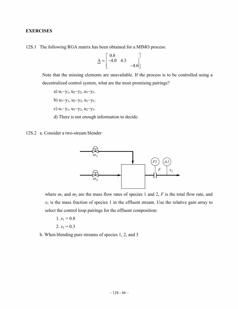
– 12S - 86 –
EXERCISES
12S.1 The following RGA matrix has been obtained for a MIMO process:
Λ = −−
0.84 0 4 3
4 6. .
.
Note that the missing elements are unavailable. If the process is to be controlled using a
decentralized control system, what are the most promising pairings?
a) u1−y1, u2−y2, u3−y3.
b) u3−y1, u2−y2, u1−y3.
c) u1−y1, u3−y2, u2−y3.
d) There is not enough information to decide.
12S.2 a. Consider a two-stream blender
where m1 and m2 are the mass flow rates of species 1 and 2, F is the total flow rate, and
x1 is the mass fraction of species 1 in the effluent stream. Use the relative gain array to
select the control loop pairings for the effluent composition:
1. x1 = 0.8
2. x1 = 0.3
b. When blending pure streams of species 1, 2, and 3
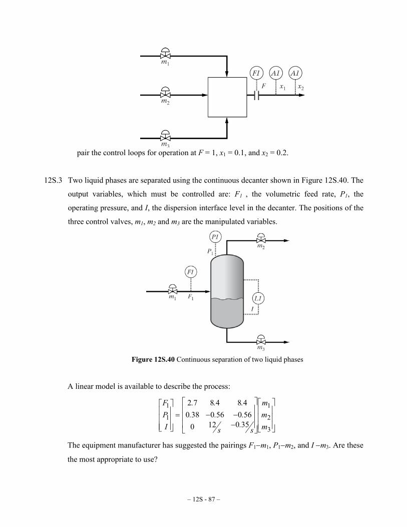
– 12S - 87 –
pair the control loops for operation at F = 1, x1 = 0.1, and x2 = 0.2.
12S.3 Two liquid phases are separated using the continuous decanter shown in Figure 12S.40. The
output variables, which must be controlled are: F1 , the volumetric feed rate, P1, the
operating pressure, and I, the dispersion interface level in the decanter. The positions of the
three control valves, m1, m2 and m3 are the manipulated variables.
Figure 12S.40 Continuous separation of two liquid phases
A linear model is available to describe the process:
FPI s s
mmm
1
1
1
2
3
2 7 8 4 8 40 38 0 56 0 56
0 12 0 35
= − −
−
. . .. . .
.
The equipment manufacturer has suggested the pairings F1−m1, P1−m2, and I −m3. Are these
the most appropriate to use?

– 12S - 88 –
Hint: 2 7 8 4 8 40 38 0 56 0 56
0 12 0 35
0 12 1 8 00 0023 0 016 0 0810 079 0 56 0 081
1. . .. . .
.
. .. . .. . .
− −−
= −− −
−
s s
ss
12S.4 In a recent publication, a decentralized control system was proposed for an experimental
reactor involving heat integration between two sections of the reactor. The manipulated
variables available for control are the heat duties to the two sections, Qp and Qc. The control
system is intended to regulate the operating temperatures in the two sections, Tp and Tc. The
authors developed a detailed nonlinear model of the process that, after linearization, gives
++
+
++
++++
+
=
c
p
c
p
sss
ss
sssss
TT
14813335148
14813333
14813330
14813337295
22
22
They tuned simple PI controllers, and found that the closed-loop response of the overall
system became faster and less oscillatory when they increased the controller gains. Use the
dynamic RGA to explain this observation.
12S.5 Reproduce the DC map in Figure 12S.11 for the Shell process.
12S.6 Three component parts were given by Weitz (1994) for the FS configuration of the heat-
integrated distillation columns in Figure 12.2. His linearized models are, for the high-
pressure column,
=
−−−−−
+−−−
−
FH
H
RH
H
....e.e..e.e....
sCH
BH
DH
xF
QL
Qxx
s.s.s.
s.
0280000308610001044910410219704701700003047110180
1111 202021
84
And for the low-pressure column,
=
−−−
−
−−
+
FL
L
L
RL
e.e.e..e....
sBL
DL
xFL
Q
xx
s.s.s.
s.
303041
96
483103400480745616800010018501121
1161
and for the feed splitter (pure gain),

– 12S - 89 –
−=
F
LH
FL
L
FH
H
xF
FF
..
..
xF
xF
100051007211100049007211
.
It can be assumed that all of the inputs are nominally at 50% of their full ranges. The
nominal values of the inputs are taken as LH = LL = 11 kmol/min, QRH = 0.205×10⁶
kcal/min, FH/FL = 0.49. The maximum disturbance magnitudes are taken as ∆F = 18
kmol/min and ∆xF = 0.2 (±20% of full range). Using these models, and noting the
interconnections between the component parts in Figure 21.13(a), reproduce the DC contour
maps in Figure 21.17 for the FS configuration.
12S.7 Two component parts were given by Weitz (1994) for the LSR configuration of the heat-
integrated distillation columns in Figure 12.2. His linearized models are, for the high-
pressure column,
=
−−−−−−−−
+−
−−−−
RH
H
L
BL
BL
.....
....e.
.e.e.e.e.
sCH
DH
BH
QLBTx
Qxx
s.
s.s.s.s.
87200008000020013004505511023000100270154042530220013004701361
1141 36
41202020
and for the low-pressure column,
=
−−−−−
−−
+−−−
−−−
−−−
−
F
RL
L
e.e..e.e.e..e.
e.e..e.e...
s
L
BL
BL
DL
xF
QL
BTxx
s.s.s.
s.s.s.
s.s.s.
s.
101041
101041
101041
98
08519980511291309636144005502720
29710050772101001310001210210
1181
.
It can be assumed that all of the inputs are nominally at 50% of their full ranges. The
nominal values of the inputs are taken as LH = LL = 11 kmol/min, QRH = 0.205×10⁶
kcal/min, FH/FL = 0.49. The maximum disturbance magnitudes are taken as ∆F = 18
kmol/min and ∆xF = 0.2 (±20% of full range). Using these models, and noting the
interconnections between the component parts in Figure 12S.13(c), reproduce the DC
contour maps in Figure 12S.17 for the LSR configuration.

– 12S - 90 –
12S.8 A product P is produced by two sequential exothermic reactions, A→B→P, with an
additional endothermic reaction of B leading to an unwanted product X. These reactions are
carried out in a jacketed CSTR, whose material and energy balances are
( ) ( )C q C C k T CA A A A= − − ⋅0 1
( ) ( ) ( )C qC k T C k T C k T CB B A B B= − + ⋅ − ⋅ − ⋅1 2 3
( )C qC k T CP P B= − + ⋅2
( ) ( ) ( ) ( )( )[ ]BAcCHTkHTkCHTkTTqT
P332211
10 ∆+∆+⋅∆−−=
ρ
−− ⋅⋅
JPc
AVU TTρ
( )
−+−= ⋅⋅JTTJTJTJqT
PcAVU
J ρ0
with reaction rate constants
( )k T k
E
Tii i
i= ⋅−
=0 1 2 3exp , , ,
The controlled variables are the concentration of P in the reactor effluent, CP, and the
reactor temperature, T. The manipulated variables are the feed flow rate, q, and the jacket
coolant flow rate, qJ. The process disturbances are the feed concentration of A, CA0, and the
feed temperature, T0. Additional information is given in Table 12S.13.
Table 12S.13 Process information for Exercise 12S.8.
Variable Value Variable Value
CP [M] 1.00 k10 [min-1] 1.169×10¹⁰ T [K] 353.15 k20 [min-1] 1.445×10¹¹ q [min-1] 0.15 k30 [min-1] 1.689×10¹¹ qJ [min-1] 0.10 E1 [K] 9000
CA0 [M] 5.00 E2 [K] 9500 T0 [K] 343.15 E3 [K] 9800 TJ0 [K] 288.15 ∆H1 [KJ/mol] -40
UVA K lKJ
⋅
⋅
min
0.225 ∆H2 [KJ/mol] -20
ρcP [KJ/K] 1.00 ∆H3 [KJ/mol] 120
– 12S - 91 –
Using the model and Table 12S.13, compute the steady-state RGA and DC. You
may assume that the disturbances in the feed concentrations are limited to within ±1M and
those of the feed temperature to ±5 K, and that the manipulated variables are nominally
midway between their lower and upper bounds. Based on these computations, answer the
following questions: a. What are the appropriate pairings to use for decentralized control? b.
What is the worst possible combination of disturbances in T0 and CA0?
Related Documents