List of Contents 1 LIST OF CONTENTS CHAPTER 1 INTRODUCTION................................................... 16 1.1 TRANSMISSION LINE ELEMENTS .................................... 16 1.1.1 Insulators .................................................................. 16 1.1.2 ADSS Cable ................................................................ 17 1.2 LOW CURRENT DISCHARGES ........................................ 18 1.2.1 Electric Fields on Transmission Lines .............................. 18 1.2.2 Low Current Discharges on Insulators ............................ 19 1.2.3 Low Current Discharges on ADSS Cables ........................ 20 1.3 OBJECTIVES ........................................................... 22 CHAPTER 2 BACKGROUND ..................................................... 23 2.1 COMPOSITE INSULATORS ............................................ 23 2.2 ADSS CABLE ......................................................... 25 2.3 SURFACE AGEING MECHANISMS .................................... 27 2.4 PHYSICS OF LOW CURRENT DISCHARGES .......................... 30 2.4.1 Corona ...................................................................... 30 2.4.1.1 Corona from Metals ......................................................... 30 2.4.1.2 Corona from Water Drops ................................................. 31 2.4.2 Dry-band Arcs ............................................................ 33 2.4.3 Flashover ................................................................... 34 2.5 ARCING DAMAGES ON INSULATORS AND ADSS CABLES ......... 37 2.6 PREVIOUS EXPERIMENTS ON LOW CURRENT DISCHARGES ....... 39 2.6.1 Tests Arrangement ...................................................... 39 2.6.1.1 Testing with Inclined Samples with Contaminant Flow........... 39 2.6.1.2 Discharges between Water Drops....................................... 40 2.6.1.3 Non-shedded Insulator Core in a Salt-fog Chamber .............. 40 2.6.1.4 Dry-band Arcs under Water-spray on a Rod......................... 41 2.6.2 Results Analysis .......................................................... 42 2.6.2.1 Leakage Current .............................................................. 42 2.6.2.2 Arc Voltage..................................................................... 43 2.6.2.3 Arc Resistance ................................................................ 43 2.6.2.4 Arc Length...................................................................... 44 2.6.2.5 Arc Power ....................................................................... 45 2.7 PREVIOUS SIMULATION OF ELECTRICAL DISCHARGES ............ 46 2.7.1 Electrical Modelling of Arcs ........................................... 46 2.7.2 Thermal Modelling of Arcs ............................................ 48 2.8 SUMMARY ............................................................. 49

Welcome message from author
This document is posted to help you gain knowledge. Please leave a comment to let me know what you think about it! Share it to your friends and learn new things together.
Transcript

List of Contents
1
LIST OF CONTENTS
CHAPTER 1 INTRODUCTION................................................... 16
1.1 TRANSMISSION LINE ELEMENTS ....................................16 1.1.1 Insulators ..................................................................16 1.1.2 ADSS Cable................................................................17
1.2 LOW CURRENT DISCHARGES ........................................18 1.2.1 Electric Fields on Transmission Lines ..............................18 1.2.2 Low Current Discharges on Insulators ............................19 1.2.3 Low Current Discharges on ADSS Cables ........................20
1.3 OBJECTIVES...........................................................22 CHAPTER 2 BACKGROUND..................................................... 23
2.1 COMPOSITE INSULATORS ............................................23 2.2 ADSS CABLE .........................................................25 2.3 SURFACE AGEING MECHANISMS ....................................27 2.4 PHYSICS OF LOW CURRENT DISCHARGES..........................30
2.4.1 Corona ......................................................................30 2.4.1.1 Corona from Metals ......................................................... 30 2.4.1.2 Corona from Water Drops ................................................. 31
2.4.2 Dry-band Arcs ............................................................33 2.4.3 Flashover ...................................................................34
2.5 ARCING DAMAGES ON INSULATORS AND ADSS CABLES.........37 2.6 PREVIOUS EXPERIMENTS ON LOW CURRENT DISCHARGES .......39
2.6.1 Tests Arrangement ......................................................39 2.6.1.1 Testing with Inclined Samples with Contaminant Flow........... 39 2.6.1.2 Discharges between Water Drops....................................... 40 2.6.1.3 Non-shedded Insulator Core in a Salt-fog Chamber .............. 40 2.6.1.4 Dry-band Arcs under Water-spray on a Rod......................... 41
2.6.2 Results Analysis ..........................................................42 2.6.2.1 Leakage Current.............................................................. 42 2.6.2.2 Arc Voltage..................................................................... 43 2.6.2.3 Arc Resistance ................................................................ 43 2.6.2.4 Arc Length...................................................................... 44 2.6.2.5 Arc Power....................................................................... 45
2.7 PREVIOUS SIMULATION OF ELECTRICAL DISCHARGES ............46 2.7.1 Electrical Modelling of Arcs ...........................................46 2.7.2 Thermal Modelling of Arcs ............................................48
2.8 SUMMARY .............................................................49

List of Contents
2
CHAPTER 3 EVIDENCE OF LONG TERM LOW CURRENT AGEING ...... 51
3.1 INTRODUCTION .......................................................51 3.2 ELECTRIC FIELD CALCULATION......................................51
3.2.1 Modelling Approach .....................................................51 3.2.2 Modelling Results ........................................................52
3.3 VISUAL OBSERVATION FROM RECOVERED CABLE .................54 3.4 CONTACT ANGLE MEASUREMENT....................................55 3.5 CORRELATION OF CONTACT ANGLE AND CURRENT WITHIN A SPAN
.........................................................................57 3.6 SUMMARY .............................................................59
CHAPTER 4 LOW CURRENT ARC COMPRESSION.......................... 60
4.1 THE ARC COMPRESSION PHENOMENON ............................60 4.2 ARC COMPRESSION SITUATIONS....................................61
4.2.1 Arc Compression on Inclined Surface with Water Film.......61 4.2.2 Arc Compression under Wind and Rain Environment.........62
CHAPTER 5 EXPERIMENTAL ................................................... 64
5.1 TESTING IN A FOG ENVIRONMENT ..................................64 5.1.1 Introduction ...............................................................64 5.1.2 Test Arrangement .......................................................64 5.1.3 Test Procedure............................................................66
5.1.3.1 Arc Formation Test .......................................................... 66 5.1.3.2 Arc Growth Test .............................................................. 67 5.1.3.3 Fog Comparison Test ....................................................... 68
5.1.4 Test Results ...............................................................69 5.1.4.1 Arc Formation Test .......................................................... 69 5.1.4.2 Arc Growth Test .............................................................. 72 5.1.4.3 Fog Comparison Test ....................................................... 75
5.1.5 Results Analysis ..........................................................76 5.1.5.1 Change of Material Surface Property in Fog Environment....... 76 5.1.5.2 Comparison between Arcs with Different Current Levels ........ 77 5.1.5.3 Comparison between Clean-fog and Salt-fog Environment ..... 82
5.2 TESTING WITH INCLINED SAMPLES .................................84 5.2.1 Introduction ...............................................................84 5.2.2 Test Arrangement .......................................................84 5.2.3 Test Procedure............................................................86 5.2.4 Test Results ...............................................................86

List of Contents
3
5.2.5 Results Analysis ..........................................................90 5.2.5.1 Arc Length...................................................................... 90 5.2.5.2 Breakdown Voltage.......................................................... 91 5.2.5.3 Arcing Period .................................................................. 92 5.2.5.4 Arc Current Peak ............................................................. 93 5.2.5.5 V-I Characteristics for Arc Compression .............................. 93 5.2.5.6 Arc Resistance and Resistivity ........................................... 94 5.2.5.7 Arc Power....................................................................... 96 5.2.5.8 Arc Energy ..................................................................... 97 5.2.5.9 Energy Density................................................................ 99
5.3 TESTS BETWEEN WATER DROPS .................................. 101 5.3.1 Introduction ............................................................. 101 5.3.2 Test Arrangement ..................................................... 102 5.3.3 Test Procedure.......................................................... 103 5.3.4 Test Results ............................................................. 104
5.3.4.1 Arc Stability.................................................................. 104 5.3.4.2 Arc Length.................................................................... 105
5.3.5 Results Analysis ........................................................ 107 5.3.5.1 Breakdown Voltage........................................................ 107 5.3.5.2 Arc Current Peak ........................................................... 108 5.3.5.3 Arcing Period ................................................................ 109 5.3.5.4 Arcing Energy ............................................................... 110 5.3.5.5 Energy Density.............................................................. 110
5.4 TESTS WITH ARTIFICIAL WIND AND RAIN ....................... 113 5.4.1 Introduction ............................................................. 113 5.4.2 Wind Test Arrangement ............................................. 113 5.4.3 Test Procedure.......................................................... 115
5.4.3.1 Investigation of Unstable Discharges to Stable Arc Transition..... .................................................................................. 115 5.4.3.2 Stable Arc to Arc Compression Transition .......................... 116
5.4.4 Test Results ............................................................. 117 5.4.4.1 Unstable Discharges become Stable as a Result of Wind...... 117 5.4.4.2 Stable Arc to Arc Compression by Wind Effect.................... 119
5.4.5 Results Analysis ........................................................ 121 5.4.5.1 Energy Trend from Unstable Discharge to Stable Arc .......... 121 5.4.5.2 Energy Trend from Stable Arc to Arc Compression.............. 123 5.4.5.3 Effect on Arcing Activities of Different Wind and Rain Intensity... .................................................................................. 124 5.4.5.4 Energy Density from Unstable Discharges to Stable Arcs ..... 126 5.4.5.5 Energy Density against Arc Length During the Arc Compression . .................................................................................. 127
5.5 SUMMARY ........................................................... 129
List of Contents
4
CHAPTER 6 SIMULATIONS OF LOW CURRENT ARCS................... 132
6.1 MODELLING OF STABLE DRY-BAND ARCS........................ 132 6.1.1 Double Sinusoidal Model............................................. 132
6.1.1.1 Double Sinusoidal Model from Experiment Results .............. 132 6.1.1.2 Modelling Parameterization Based on Testing in a Fog Environments ........................................................................... 135 6.1.1.3 Modelling Results for Stable Arcs ..................................... 139
6.1.2 PSCAD Simulation ..................................................... 143 6.1.2.1 Simulation Circuit for Stable Arcs from Testing in a Fog Environment............................................................................. 143 6.1.2.2 Circuit Breaker for Arc Ignition and Extinction.................... 144 6.1.2.3 Simulation of Instantaneous Arc Resistance....................... 145 6.1.2.4 PSCAD Simulation Results for Stable Arc........................... 147
6.2 MODELLING OF ARC COMPRESSION .............................. 151 6.2.1 Double Sinusoidal Model for Arc Compression................ 151
6.2.1.1 Modelling Parameterization Based on Testing with Inclined ........ Samples...................................................................... 151 6.2.1.2 Modelling Results for Arc Compression.............................. 154
6.2.2 PSCAD Simulation for Arc Compression ........................ 158 6.2.2.1 Simulation Circuit and ‘BRK’ Control Circuit ....................... 158 6.2.2.2 Simulation of Instantaneous Arc Resistance for Arc Compression .................................................................................. 159 6.2.2.3 PSCAD Simulation Result for Arc Compression ................... 161
6.2.3 Arc Energy and Energy Density during Arc Compression .165 6.3 MODELLING OF UNSTABLE DISCHARGES ......................... 167
6.3.1 PSCAD Simulation Circuit for Unstable Discharges.......... 167 6.3.2 Simulation of Unstable Discharge Resistance with Vibration Unit .............................................................................. 168 6.3.3 PSCAD Simulation Results for Unstable Discharges......... 170 6.3.4 Arc Energy and Energy Density from Unstable Discharges to Stable Arcs.......................................................................... 172
6.4 MODELLING OF THERMAL DYNAMICS OF ARCS .................. 175 6.4.1 Triple Cylinder Model ................................................. 175 6.4.2 Thermal Flow Calculation............................................ 177 6.4.3 Thermal Flow for Dry-band Arc Compression ................. 179 6.4.4 Modelling Parameterization for the Triple Cylinder Model. 180 6.4.5 Calculation Results from Triple Cylinder Model............... 183
6.5 SUMMARY ........................................................... 188

List of Contents
5
CHAPTER 7 DISCUSSION .................................................... 189
7.1 LONG-TERM LOW CURRENT AGEING WITHOUT DISCHARGES .. 189 7.2 THE PROPERTIES OF LOW CURRENT ARCS....................... 189
7.2.1 Arc Stability and Current ............................................ 189 7.2.2 Arc Length ............................................................... 191 7.2.3 Breakdown Voltage.................................................... 192 7.2.4 Arcing Period ............................................................ 193 7.2.5 Arc Resistance and Resistivity ..................................... 193 7.2.6 Arc Energy and Energy Density ................................... 194
7.3 MODELLING AND SIMULATION OF LOW CURRENT ARCS ........ 195 7.3.1 Modelling Parameter Extraction from Experimental Results... .............................................................................. 195 7.3.2 Modelling Assumptions............................................... 195
CHAPTER 8 CONCLUSION.................................................... 198 CHAPTER 9 FUTURE WORK.................................................. 201 REFERENCES .................................................... 203 APPENDIX 1: MATLAB PROGRAMS......................... 207
APPENDIX 1.1 ............................................................. 207 APPENDIX 1.2 ............................................................. 207 APPENDIX 1.3 ............................................................. 209
APPENDIX 2: LIST OF PUBLICATIONS .................... 210

List of Figures
6
LISTS OF FIGURES Figure 1-1: Images of insulators on overhead transmission lines ....................... 17 Figure 1-2: The location of ADSS cable on overhead transmission lines ........... 18 Figure 1-3: An example of electric field distribution around a typical L7
suspension tower on a 132 kV transmission line................................ 19 Figure 1-4: Surface joule heating on an arbitrary hydrophilic insulator shape
which is polluted and wetted ................................................................... 20 Figure 1-5: Schematic showing the relationship between the induced voltage,
current and dry-band area on ADSS cable........................................... 21 Figure 2-1: General arrangement of a composite insulator................................... 23 Figure 2-2: Schematic of the structure of ADSS cables ......................................... 25 Figure 2-3: Chemical reactions in RTVSR covered composite insulator surface
by dry-band arc discharges ..................................................................... 29 Figure 2-4: An evidence of corona cutting damage on composite insulator...... 30 Figure 2-5: Equipotentials surrounding a hemispherical water drop on a
polymer with a uniform E-field applied prior to the introduction the water drop .................................................................................................... 32
Figure 2-6: Behaviour of a water droplet under AC voltage.................................. 32 Figure 2-7: Schematic of dry-band arcing on a contaminated (polluted)
insulator ........................................................................................................ 36 Figure 2-8: Test arrangement for measurement of voltage, current and
temperature distribution on inclined sample surface......................... 39 Figure 2-9: Test arrangement for measurement of electrical discharges
between water drops ................................................................................. 40 Figure 2-10: Test arrangement in salt-fog chamber with insulator core............ 41 Figure 2-11: Test arrangement of dry-band arcing under the spray system on
the ADSS cable ........................................................................................... 41 Figure 2-12: Test arrangement of dry-band arcing under the spray system on
the ADSS cable ........................................................................................... 43 Figure 2-13: Arc resistance analysis from voltage and current signals .............. 44 Figure 2-14: The relationship between arc length and arc current ..................... 44 Figure 2-15: Instant arc power calculation based on arc voltage and arc
current........................................................................................................... 45 Figure 2-16: Equivalent circuit of experiment setup ............................................... 46 Figure 2-17: Simulation of voltage and current waves comparing with
experimental results (breakdown voltage 12 kV, arc length 1.45 cm)........................................................................................................................ 47
Figure 2-18: Simulation of current and voltage curves of arcs with instantaneous arc resistance ................................................................... 47
Figure 2-19: Two-solid thermal model and three-solid thermal model for high current short distance arcs ...................................................................... 48
Figure 3-1: The parameters of L7 tower for electric field calculation (132kV) . 53 Figure 3-2: Current magnitudes along the DM27-DM28 ADSS cable span ......54 Figure 3-3: Example of visual inspected cable segments ...................................... 55 Figure 3-4: Contact angle results from a) whole cable span DM30-DM31, b)
only UV aged cable, and c) only discharge aged cable ..................... 56 Figure 3-5: Correlation of contact angle and current in DM30-DM31 ................. 57 Figure 3-6: The trend line of contact angle against leakage current .................. 58

List of Figures
7
Figure 4-1: Typical dry-band arc on insulating surface with moisture................ 60 Figure 4-2: Dry-band arc compression on inclined surface between water films
........................................................................................................................ 61 Figure 4-3: Inclined surface for arc compression on power transmission lines 62 Figure 4-4: Dry band arc compression under wet rain and wind conditions ..... 63 Figure 5-1: Test arrangement of Testing in a Fog Environment........................... 65 Figure 5-2: Voltage and current curves from stage 1 to stage 5 in the clean-fog
environment................................................................................................. 71 Figure 5-3: Summary of phase shift and current increase from stage 1 to stage
3 in the clean-fog environment............................................................... 72 Figure 5-4: The transformation from several arcs to one single arc ................... 72 Figure 5-5: Dry-band arcs for different current levels from 1.5 mA to 4.0 mA in
salt-fog environment ................................................................................. 74 Figure 5-6: Arc images in both clean-fog and salt-fog environment................... 75 Figure 5-7: Voltage and current behaviours for arcs in different fog
environments............................................................................................... 75 Figure 5-8: Electrical model of silicone rubber sample surface ............................ 76 Figure 5-9: Identification of arcing period and breakdown voltage of 1.5 mA arc
........................................................................................................................ 77 Figure 5-10: The relationship between breakdown voltage, source voltage peak
and arc length ............................................................................................. 78 Figure 5-11: The relationship between arcing period and arc length.................. 79 Figure 5-12: V-I (voltage against current) characteristics of dry-band arcs for
different current levels from 1.5 mA to 4.0 mA.................................. 80 Figure 5-13: Instantaneous arc resistances of 2.5 mA peak current arcing for
four consecutive half power cycles......................................................... 81 Figure 5-14: Instantaneous arc resistances of arcs in different current levels. 81 Figure 5-15: Instantaneous arc resistivity of arcs in different current levels ... 82 Figure 5-16: Test arrangement of Testing with Inclined Samples ....................... 85 Figure 5-17: Experimental results of current and voltage traces for inclined arc
compression along with images showing arc physical lengths........ 90 Figure 5-18: The relationship between arc length and slope angle..................... 91 Figure 5-19: The relationship between breakdown voltage and arc length....... 92 Figure 5-20: The relationship between arcing period and arc length.................. 92 Figure 5-21: The relationship between arc current peak and arc length ........... 93 Figure 5-22: V-I characteristics of dry-band arcs for inclined arc compression94 Figure 5-23: Instantaneous arc resistances of inclined compressed arcs with
different arc lengths................................................................................... 95 Figure 5-24: Instantaneous arc resistivity of inclined compressed arcs with
different arc lengths................................................................................... 95 Figure 5-25: Instantaneous arc power calculation based on 5° slope angle..... 97 Figure 5-26: Instantaneous arc power calculation with a range of slope angles
........................................................................................................................ 97 Figure 5-27: Arc energy calculation based on the instantaneous arc power..... 98 Figure 5-28: Experimental results of arc energy against arc length for different
arcs in Testing with Inclined Samples ................................................... 99 Figure 5-29: Experimental results of energy density against arc length for
different arcs in Testing with Inclined Samples ................................ 100 Figure 5-30: Test arrangement of water drops test.............................................. 102 Figure 5-31: Three different cases of discharges between water drops. ......... 104

List of Figures
8
Figure 5-32: Voltage and current traces with the reduction of initial distance between water drops under the different voltage levels ................ 107
Figure 5-33: Breakdown voltage for stable arcs with supply voltage levels of 10 kV, 15 kV, 20 kV and 25 kV................................................................... 108
Figure 5-34: The change of arc current peak corresponding to variable distances under the different voltage levels of 10 kV, 15 kV, 20 kV and 25 kV ................................................................................................... 109
Figure 5-35: The change of arcing period corresponding to variable distances under the different voltage levels of 10 kV, 15 kV, 20 kV and 25 kV...................................................................................................................... 109
Figure 5-36: The change of arcing period corresponding to variable distances under the different voltage levels of 10 kV, 15 kV, 20 kV and 25 kV...................................................................................................................... 110
Figure 5-37: Cylinder model for calculation of arc energy density .................... 111 Figure 5-38: The change of arcing period corresponding to variable distances
under the different voltage levels of 10 kV, 15 kV, 20 kV and 25 kV...................................................................................................................... 111
Figure 5-39: Test arrangement of Tests with Artificial Wind and Rain ............. 114 Figure 5-40: Unstable discharges become stable after wind injection.............. 119 Figure 5-41: Arc compression in 20 kV (peak) at different wind levels............ 121 Figure 5-42: Energy change from unstable discharges to stable arcs under the
20 mph wind and strong spray conditions ......................................... 122 Figure 5-43: Energy trend from unstable discharges to stable arcs under the
10 mph wind and weak spray conditions............................................ 123 Figure 5-44: Energy trend from free-growth of an arc to arc compression with
reduction in arc length ............................................................................ 124 Figure 5-45: An example of arc compression under different wind and rain
situations (20 kV, 10 mA arc) ............................................................... 126 Figure 5-46: The trend of energy density from unstable discharges to stable
arcs .............................................................................................................. 127 Figure 5-47: The trend of energy density from free arc to arc compression with
arc length ................................................................................................... 128 Figure 6-1: Double sinusoidal model based on the experimental I-t and V-t
result ........................................................................................................... 132 Figure 6-2: Simulated I-t and V-t traces from Double Sinusoidal Model
comparing with experimental results in Testing in a Fog Environment .............................................................................................. 141
Figure 6-3: Simulation circuit for stable dry-band arcs in PSCAD ..................... 143 Figure 6-4: Control Circuit of Circuit Breaker for arc ignition and extinction .. 145 Figure 6-5: Simulation circuit for instantaneous arc resistance in PSCAD....... 147 Figure 6-6: PSCAD simulation result of I-t and V-t curves for stable dry-band
arcs with different current levels .......................................................... 149 Figure 6-7: The Double Sinusoidal Model Simulated I-t and V-t traces for
variable arc lengths under different arc compression situations comparing with experimental results from Testing with Inclined Samples ...................................................................................................... 157
Figure 6-8: Simulation circuit for arc compression in PSCAD ............................. 158 Figure 6-9: Example of control signal ‘BRK’ for different arc compression
situations .................................................................................................... 159 Figure 6-10: Example of control signal ‘BRK’ for different arc compression
situations .................................................................................................... 160

List of Figures
9
Figure 6-11: Examples of simulated arc resistance for arc lengths of 2.32, 1.94 and 1.11 cm during the arc compression ........................................... 160
Figure 6-12: PSCAD simulation result of I-t and V-t curves for arc compression with different arc lengths ....................................................................... 163
Figure 6-13: Experimental and simulation arc energy against arc length as a result of arc compression ....................................................................... 165
Figure 6-14: Experimental and simulation results of relationship between arc length and energy density charge during arc compression ........... 166
Figure 6-15: Simulation circuit for unstable discharges in PSCAD..................... 167 Figure 6-16: Control signal ‘BRK’ for simulation of unstable discharges.......... 168 Figure 6-17: Simulation result of entire unstable discharge resistance ‘BRK’. 169 Figure 6-18: Simulation circuit for entire unstable discharge resistance ......... 170 Figure 6-19: Simulation result of unstable discharges ......................................... 172 Figure 6-20: Arc energy trends from unstable discharges to stable arcs for both
PSCAD simulation and experiment results ......................................... 173 Figure 6-21: Energy density trends from unstable discharges to stable arcs for
both PSCAD simulation and experiment results ............................... 174 Figure 6-22: Triple cylinder thermal model with three distinguish zones and
corresponding power flow in every direction ..................................... 175 Figure 6-23: Energy flow calculation for one cylinder model (each arcing zone)
...................................................................................................................... 177 Figure 6-24: Thermal modelling of dry-band arc compression ........................... 180 Figure 6-25: Result of calculated power radiation from zone 1, zone 2 and zone
3 to cathode (PK), anode (PA), and insulation material surfaces (P1S, P2S, P3S) ........................................................................................ 186
Figure 6-26: Modelling results of dry-band arcing energy for different radiation directions .................................................................................................... 187
List of Tables
10
LIST OF TABLES Table 2-1: Hampton’s criterion for dry-band arc extension ......................... 34 Table 2-2: Hampton’s criterion as a judgment tool for dry-band arc extension
on ADSS cable surface........................................................... 35 Table 3-1: Modelling parameter Ia for different levels of stable dry-band arcs52 Table 5-1: Summary of arc stability in different voltage level and drop gap 105 Table 5-2: The transformation period from unstable discharges to stable arcs
under different wind and rain situations ................................. 125 Table 6-1: Modelling parameter Ia for different levels of stable dry-band arcs
........................................................................................ 136 Table 6-2: Modelling parameter Ua for different levels of stable dry-band arcs
........................................................................................ 137 Table 6-3: Modelling parameter Ut1 for different levels of stable dry-band arcs
........................................................................................ 137 Table 6-4: Modelling parameter Ut2 for different levels of stable dry-band arcs
........................................................................................ 138 Table 6-5: Modelling parameter t1 for different levels of stable dry-band arcs
........................................................................................ 138 Table 6-6: Modelling parameter t2 for different levels of stable dry-band arcs
........................................................................................ 138 Table 6-7: Modelling parameter ωu for different levels of stable dry-band arcs
........................................................................................ 139 Table 6-8: Modelling parameter ωi for different levels of stable dry-band arcs
........................................................................................ 139 Table 6-9: Input parameters for instantaneous arc resistance in PSCAD
simulation for different current levels of dry-band arc .............. 146 Table 6-10: Correlation coefficients ‘r’ for current and voltage curves of dry-
band arcs between experimental results from the Testing in a Fog Environment, modelling results from Double Sinuoidal Model, and simulation results from PSCAD.............................................. 150
Table 6-11: Correlation coefficients ‘r’ for current and voltage curves of arc compression between experimental results from Testing with Inclined Samples, modelling results from Double Sinuoidal Model, and simulation results from PSCAD........................................ 164
Table 6-12: Calculated coefficients for Triple Cylinder Model based on Testing with Inclined Samples ......................................................... 183
Table 6-13: Energy radiation from dry-band arcing to surroundings in a power cycle................................................................................. 186

Abstract
11
ABSTRACT
Ageing of outdoor insulation under low leakage currents are concerns for
safety and reliability in transmission line operations. Overhead line
elements such as insulators and ADSS (All Dielectric, Self-Supporting)
cables are subject to electric fields, resultant leakage currents, and
resulting surface discharges such as coronas and dry-band arcs. Under
certain conditions, the normally benign long-term low current ageing
effect may transform to more severe ageing forms, having a detrimental
impact on the insulation materials and creating high rates of unexpected
failures.
In this thesis, a series of experimental studies are reported which have
created low current discharges under variable electrical and
environmental conditions. The electrical properties of resulting arcs are
investigated and their impact on the insulation materials is analyzed.
Based on the test results, new modelling approaches have been
developed for the simulation of dry-band arcing activity. The respective
‘Double Sinusoidal Model’ and ‘PSCAD simulation’ are able to simulate
the voltage and current traces of low current arcs, while the ‘Triple
Cylinder Model’ is used to analyze the heat flow around the arcing region.
Based on both experiment and simulation, the phenomenon of ‘dry-band
arc compression’ is reproduced. Research confirms previous suggestions
that such a compression process may lead to more aggressive damage
on insulation surfaces, and could possibly accelerate the long-term
ageing effect into a short-term hazard. As a result, this thesis supports
the argument that processes controlling insulation lifetime may not be
continual and gradual, but are determined by extreme events such as
the occurrence of dry-band arc compression.

Declaration
12
DECLARATION
That no portion of the work referred to in the thesis has been submitted
in support of an application for another degree or qualification of this or
any other university or other institute of learning.

Copyright Statement
13
COPYRIGHT STATEMENT
The following four notes on copyright and the ownership of intellectual
property rights must be included as written below:
I. The author of this thesis (including any appendices and/or schedules to this thesis) owns certain copyright or related rights in it (the “Copyright”) and s/he has given The University of Manchester certain rights to use such Copyright, including for administrative purposes.
II. Copies of this thesis, either in full or in extracts and whether in hard
or electronic copy, may be made only in accordance with the Copyright, Designs and Patents Act 1988 (as amended) and regulations issued under it or, where appropriate, in accordance with licensing agreements which the University has from time to time. This page must form part of any copies made.
III. The ownership of certain Copyright, patents, designs, trade marks
and other intellectual property (the “Intellectual Property”) and any reproductions of copyright works in the thesis, for example graphs and tables (“Reproductions”), which may be described in this thesis, may not be owned by the author and may be owned by third parties. Such Intellectual Property and Reproductions cannot and must not be made available for use without the prior written permission of the owner(s) of the relevant Intellectual Property and/or Reproductions.
IV. Further information on the conditions under which disclosure,
publication and commercialisation of this thesis, the Copyright and any Intellectual Property and/or Reproductions described in it may take place is available in the University IP Policy (see http://www.campus.manchester.ac.uk/medialibrary/policies/intellectual-property.pdf), in any relevant Thesis restriction declarations deposited in the University Library, The University Library’s regulations (see http://www.manchester.ac.uk/library/aboutus/regulations) and in The University’s policy on presentation of Theses.

Chapter 1: Introduction
14
ACKNOWLEDGEMENTS
I would like to give my sincere appreciation to Prof. Simon Rowland,
who was my PHD supervisor from 2007 to 2010 (also my MSc
supervisor from 2006 to 2007), for his remarkable guidance and kindly
help. With his academic effort and financial support, I managed to
publish two journal papers (another two are being written for
submission), five conference papers, and attended several electrical
insulation conferences held in United Kingdom, Canada, South Africa
and United States. From his inspiration, I decided to continue working in
the Electrical Power Sector as a Power System Engineer in National Grid
UK.
I wish to thank National Grid, who is the sponsor of my PhD project, for
their financial and technical support in this work for three years, and the
permission to publish academic papers.
I would like to express my sincere appreciation to Miss. Xiaolei Liu, who
is my fiancée, for her positive attitude to encourage me continuously to
pursue the PhD degree in this University. We met and fell in love during
our MSc study and now she has been working in Lloyds Banking Group
in London for two years. Thanks indeed for her understanding to allow
me spend most of time doing research in Manchester, and apologize for
insufficient accompany with her during this period.
Finally, my sincere gratitude is given to my beloved parents for
motivating me to study in Manchester, for their encouragement and
financial support. Although there are 5,000 miles from China to UK, our
hearts are always closed to each others.

Chapter 1: Introduction
15
LIST OF ABBREVIATIONS
AC Alternative current
ACF Autocorrelation function
ADSS All dielectric, self-supporting
A/D Analog-to-digital
EPR Ethylene propylene rubber
FFT Fast Fourier transforms
I-t Current against time
PDMS Polydimethylsiloxane
PE Polyethylene
PET Polyethylene terephthalate
RMS Root mean square
RTVSR Room-temperature vulcanized silicone rubber
UV Ultra-violet
V-I Voltage against current
V-t Voltage against time
XLPE Cross-linked polyethylene

Chapter 1: Introduction
16
1CHAPTER 1
INTRODUCTION Ageing of outdoor insulation under low leakage currents are long-term
effects in power systems. On overhead transmission lines, elements
such as insulators, conductors and communication cables may suffer
from this form of ageing. Under some circumstances, low current
discharges such as corona, dry-band arcing or even flashover may
develop on insulation surfaces, leading to erosion or damage thereby
reducing the quality and reliability of insulation materials. This may
eventually lead to mechanical failures of insulators and conductors, and
dielectric failures of overhead line insulation. There is evidence to
suggest high rates of transmission line faults.
1.1 TRANSMISSION LINE ELEMENTS
1.1.1 INSULATORS
The first high voltage insulator utilized in a power transmission line was
invented in 1882. Development resulted in rapid growth over the 19th
and 20th centuries [1]. The history of composite insulators dates back to
the 1940s, when organic materials were applied in indoor insulator
manufacture [2]. For the last thirty years, composite insulators have
been increasingly used in modern power transmission systems,
achieving excellent supporting and dielectric functions [1].

Chapter 1: Introduction
17
a) 500kV line using composite insulators, b) a 230kV line using cap and pin
porcelain insulators [1], and c) Main structure of a composite insulator
Figure 1-1: Images of insulators on overhead transmission lines
Insulators have two main functions, which are mechanical support and
dielectric insulation respectively. The mechanical function is to hold the
conductors, sustain their weight stress on suspension towers (Figure
1-1), or their tension stress on tension towers. Dielectric supports must
provide an electrical barrier between the metallic tower and
transmission conductors in order to avoid flashover [3].
1.1.2 ADSS CABLE
All-dielectric, self-supporting (ADSS) cables have been proven as a
standard method to install the optical fibres onto high voltage
transmission lines, for the purposes of high-bandwidth network control
and communication [4].
Figure 1-2 a) shows the construction of a typical twin circuit tower (UK)
and the location of an ADSS cable, suspended independently of the
phase conductors. The relative position of the ADSS cable between the
six phase conductors may vary significantly between a tension tower
and a suspension tower, because these two kinds of towers have
different cable clamping locations. On a tension tower, the ADSS cable is
installed between the bottom two conductors. On a suspension tower
the ADSS is clamped roughly midway between the bottom four

Chapter 1: Introduction
18
conductors. In addition, because of the different mechanical properties
of the conductors and the ADSS cable, they are strung with very
different sags. This sag difference along with the clamping positions
leads to changes in the relative position of an ADSS cable relative to the
phase conductors between two such towers as illustrated in Figure 1-2
b).
Figure 1-2: The location of ADSS cable on overhead transmission lines
1.2 LOW CURRENT DISCHARGES
1.2.1 ELECTRIC FIELDS ON TRANSMISSION LINES
On the overhead transmission line systems, an electrical field is created
by the distributed capacitance and leakage currents between the phase
conductors, the earth wire, the tower, insulators (and ADSS cable if
applicable). Figure 1-3 gives an example of calculated electric field
distribution around a tower. The voltage gradient varies with locations
around the tower, with 100% of phase voltage appearance at the
conductors and less than 1% of voltage near the tower and earth wire.
b) ADSS cable location in an overhead line span
a) ADSS cable location on a suspension tower

Chapter 1: Introduction
19
In addition, the electric field distribution changes across the whole span
length between towers. Therefore, a voltage gradient is generated along
the insulators or ADSS cable which drives low leakage currents on the
subject insulation surfaces.
Figure 1-3: An example of electric field distribution around a typical L7
suspension tower on a 132 kV transmission line
1.2.2 LOW CURRENT DISCHARGES ON INSULATORS
As discussed previously, because the voltage gradients are distributed
differently on insulators, leakage currents may flow on the insulator
surface. As a result, dry-band arcing activity may occur on the insulator
surface. The process is illustrated in Figure 1-4 (a part of this figure is
from [3]).

Chapter 1: Introduction
20
Figure 1-4: Surface joule heating on an arbitrary hydrophilic insulator shape
which is polluted and wetted [3]
Moisture (a water layer) can be deposited on the insulator surface due
to wet weather such as fog and rain, facilitated by any reduction of
insulator surface hydrophobicity [3]. The Joule-heating from the leakage
current causes the water layer to evaporate. The corresponding heating
density calculation indicates that the area with the maximum current
density is readily dried out. This first dry-out area may be located
around the insulator core because the current density is relatively high
there. As the water film is evaporated and becomes thinner, the surface
resistivity also increases, accelerating the drying process. Higher
resistivity leads to electric field increases. Following this effect, if the
ionization field level is met, a discharge occurs. This form of discharge is
a low current corona phenomenon. If the drying process creates a well
defined dry-band area with a gap separating two extensive water layers,
an arc may be established in the dry-band area and this is called a ‘dry-
band arc’ [5].
1.2.3 LOW CURRENT DISCHARGES ON ADSS CABLES
As shown in Figure 1-5, the electric field generated voltage gradients
will be spread along the ADSS cable suspended between towers. This
voltage gradient can be as much as tens of kilovolts dropped within

Chapter 1: Introduction
21
several metres along the cable [6]. If the surface of the cable becomes
wet and conductive, the gradient is able to induce milliamp sized
currents along its length. As the towers earth the cable via metallic
clamps, the voltage reduces to zero at both ends of cable. The shape of
current is however variable with different locations along the cable, and
may turn to zero somewhere on the span. This characteristic is not
reflected in this figure for simplification purpose.
Figure 1-5: Schematic showing the relationship between the induced voltage,
current and dry-band area on ADSS cable [6]
This current can give rise to heating on the cable. Following this heating
effect, a dry-band will consequently occur on the surface if the cable is
covered with moisture. The dry-band will possess higher impedance
than other wet parts of the cable surface. This high impedance
characteristic leads to a large voltage drop across the short section of
dry-band. Eventually the dry-band arc may be formed [6].

Chapter 1: Introduction
22
1.3 OBJECTIVES
The objective of this thesis is to investigate ageing as a result of low
surface currents for outdoor insulation on overhead transmission lines.
The electrical discharges associated with the dry-band arcing
phenomenon are the emphasis of this research. The detailed objectives
are to:
1) Understand the impact of low current ageing on transmission line
elements such as insulators and ADSS cables.
2) Understand low current dry-band arcing phenomenon on outdoor
insulation surfaces.
3) Theoretically describe the cause of dry-band arc compression;
analyze the reasons and situations for arcing compression happening.
4) Develop a series of experiments investigating low current arcs on
insulation surfaces for different environmental and electrical conditions;
experimentally study the rare but severe ageing forms of dry-band arc
compression.
5) Develop mathematical models for the simulation of dry-band arcing
and arc compression situations created in experimental work; further to
model the heat flow inside the arc and from arc to its surroundings,
especially on material surfaces.
6) Summarize the extreme ageing situations of low current arcing
compression and their impact on outdoor insulation materials, based on
both experimental and simulation work.

Chapter 2: Background
23
2CHAPTER 2
BACKGROUND
2.1 COMPOSITE INSULATORS
Figure 2-1 demonstrates the typical structure of a composite insulator
[7]. The fibreglass core is made of axially aligned glass fibres bonded
together with organic resin. This design is able to achieve a reliable
mechanical support for the suspension of transmission conductors [5].
However, this kind of fibreglass core without surface protection can not
survive outdoor, high voltage applications. The moisture contamination
and leakage current may lead to surface tracking, resulting in the
fracture failure of the fibreglass composite core [8]. In order to prevent
insulator core failure, sheds made from composite materials such as
silicone rubber or ethylene propylene rubber (EPR) are moulded on to
the fibreglass core for mainly two protection purposes. Firstly, these
sheds can protect the insulator core from penetration of water,
contamination and arcing plasma, dramatically reducing the possibility
of the fibreglass core being damaged over its long-term service. Also,
the dielectric materials of sheds can provide excellent electrical
insulation between the insulators’ upper and lower end fittings by
increasing the ‘creepage distance’ and resistivity against surface current
[3].
Figure 2-1: General arrangement of a composite insulator [7]

Chapter 2: Background
24
The main advantage of composite insulators is their excellent electrical
insulation resulting from the surface dielectric. This strength is
controlled by surface moisture and deposits [3]. Due to the low surface
energy of some composite materials such as silicone rubber [9],
composite insulators provide high hydrophobicity performance.
Furthermore, some insulator coating materials such as silicone rubber
demonstrate the ability to recover hydrophobicity after ageing [10]. As a
result of these inherent abilities to repel water, composite insulators
have a strong surface dielectric strength even when wet, so that they
can be utilized in heavily contaminated areas [11], or higher voltage
level power transmission systems [12].
Other advantages are: low weight, reduced damage possibility from
vandalism such as gunshot, reduced levels of maintenance such as
insulator washing [13], short construction periods and good
contamination performance [14].

Chapter 2: Background
25
2.2 ADSS CABLE
Typically, an ADSS cable includes optical fibres embedded in loose tubes,
a strength member and a sheath as their main parts. The structure of
such a cable is shown in Figure 2-2 a) [15]. The cable investigated in
this thesis is a ribbon-in-slot design manufactured by STC and is no
longer made [16], and this cable structure is shown in Figure 2-2 b).
a) Typical modern structure of ADSS cable cross-section [15]
b) Structure of specified ADSS cable examined in this thesis [16]
Figure 2-2: Schematic of the structure of ADSS cables
The main functions of each part of the ADSS cable are described as
follows: Optical fibres are used as the medium for communication. The
advantage of optical fibres is their inherent immunity to electromagnetic

Chapter 2: Background
26
interference. Loose tubes or slotted cores are used to house and protect
optical fibres. Loose tubes are stranded in order to provide the cable
‘excess fibre length’ to avoid optical fibres themselves being strained. In
a slotted core this excess length is provided by the undulation of the
ribbons. Typically modern ADSS cables utilize aramid yarns as strength
members. Finally a sheath is used to protect cable elements from the
environment. As long as moisture does not penetrate the cable the
internal structure does not affect the electrical performance of the cable
sheath. If the sheath is punctured and moisture penetrates the core,
discharges can occur within the cable leading to thermal and ageing
issues. Water blocking of a core is thus an essential design requirement
[4, 17, 18].

Chapter 2: Background
27
2.3 SURFACE AGEING MECHANISMS
The insulation surfaces can be influenced by their outdoor service
surroundings, as a result of environmental elements such as UV
radiation, contamination and ultimately electrical discharges such as
corona and dry-band arcing.
Solar UV radiation with wavelengths from 290 to 350 nm are incident on
insulator surfaces. The associated photon energy (about 398 kJ/mole) is
greater than the bond strength of molecules of some polymeric
materials utilized for composite insulators. As the result, the composite
surface can be degraded by UV from sunlight; furthermore, this
degradation can be accelerated with the presence of moisture [3].
Generally, contamination deposition is retained more readily on aged
composite insulators compared to porcelain insulators under the same
environment [19]. The contamination distribution on a composite
insulator has been found to be non-uniform, higher on both ends, but
lower in the middle of an insulator string [20]. The contamination
performance may depend on the profile as well as shape variation of
shed design, and also the natural cleaning effects of rainfall and wind
[3]. Some shed designs using separately moulded weather sheds may
have weak points around their radial joints when exposed to
contaminated environments [21]. Soluble contamination can increase
the wetting process over the insulator surface, which may be considered
as a contribution to the loss of hydrophobicity of insulator surface [3].
Low current electrical discharges such as corona or dry-band arcs can
also lead to chemical reactions on polymers. An investigation of room-
temperature vulcanized silicone rubber (RTVSR) under dry-band arcing
was conducted and the reasons for hydrophobicity loss of this material is
revealed in [22]: The basic polymer of RTVSR is polydimethylsiloxane

Chapter 2: Background
28
(PDMS). The molecular structure of PDMS is shown in Figure 2-3 a). The
heat from dry-band arcing probably causes scission of -CH3 groups from
Si shown in Figure 2-3 b), the scission of the polymer backbone shown
in Figure 2-3 c), as well as interchange of this backbone shown in Figure
2-3 d). The dots associated with O, Si and CH3 represent the free
radicals that scission and the interchange reaction create. In the
presence of moisture (H2O), a hydrolysis reaction may occur as
described in Figure 2-3 e) and Figure 2-3 f). The hydrolysis is followed
by oxidation of hydrocarbon groups and crosslinking of siloxane bond in
Figure 2-3 g). The increased oxygen and OH level are responsible for
creating high hydrogen bonding forces between RTVSR and water
(moisture) resulting in the rapid loss of hydrophobicity. The cross-linking
results in embrittlement of the polymer.
a) Molecular structure of PDMS b) Scission of –CH3 groups from Si
c) Scission of polymer backbone d) Interchange of backbone
e) Hydrolysis of siloxane bonds
f) Hydrolysis of hydrocarbon groups

Chapter 2: Background
29
g) Oxidation of hydrocarbon groups and crosslinking of siloxane bond
Figure 2-3: Chemical reactions in RTVSR covered composite insulator surface
by dry-band arc discharges [22]

Chapter 2: Background
30
2.4 PHYSICS OF LOW CURRENT DISCHARGES
2.4.1 CORONA
Corona is a kind of electrical discharge which can be present on
composite insulators. There are two kinds of corona summarized below:
Corona on insulator hardware is generally a concern for composite
insulators with the line voltage higher than 69 kV. This corona
particularly occurs from the metallic insulator attachment hardware
(normally the bottom hardware close to the line-end) in air or on an
insulator surface. Evidence of corona cutting on the line-end shed of an
115 kV composite insulator is shown in Figure 2-4 [3].
Figure 2-4: An evidence of corona cutting damage on composite insulator [3]
2.4.1.1 CORONA FROM METALS
The reason for corona ignition is that the voltage gradient distributed on
insulator exceeds a threshold. The initial electric field for corona
formation on a clean smooth surface in standard air density (760mm Hg
and 25°C) is 21.2 kV/cm [3]. The ‘average’ inception voltage gradient
for corona on a real object is determined by surface condition such as

Chapter 2: Background
31
roughness and contamination, as well as atmospheric effects such as
humidity and air density δ which can be calculated as [5]:
293101.3
=b
Tδ kV/cm 2-1
Where: b is air pressure (kPa) and T (K) is air temperature.
As a reference the standard atmospheric humidity is taken as 11 gm-3,
with absolute humidity varying between 1 gm-3 and 30 gm-3 [5].
Tests of aged insulators show that the ‘surface factor’ for corona
discharge has been reduced to 0.7, which represents the corona
inception potential gradient is reduced to 14.8kV/cm, 70% of its ‘ideal’
value [3].
The line voltage and radius of curvature of insulator hardware are
fundamental in determining the magnitude and distribution of
macroscopic voltage gradient are also domination factors for corona
presence [3].
2.4.1.2 CORONA FROM WATER DROPS
Water drops on insulators can also result in corona when the magnitude
of the surface electric field goes above a threshold value [23]. Windmar
[24] has defined that the electric field required for water drop corona
inception lies between 5-7 kV/cm for single or multiple droplets aligned
in the same direction. Phillips’s [25] experiment demonstrates that the
threshold value is dependent on the surface material and the volume of
water drop. He showed that the larger size of water drop, the higher
threshold electric field is required, with 8.6 kV/cm corresponding to a 50
μl water drop and 9.6 kV/mm corresponding to a 125 μl volume. There
are mainly two reasons why water drops can generate corona discharge

Chapter 2: Background
32
in electric fields: electric field enhancement [23] and water drop
deformation [26]. Electric field studies around a hemispherical water
drop on an insulating surface shows that the electric field is intensified in
the region of the water drop contacting the insulating material (Figure
2-5) [23], which may increase the electric field in this region to, or
above, the threshold value of corona. The water drop deformation is
seen under AC voltage in Figure 2-6, which may contribute to corona
generation from the tips of deformed water drops, where the curvature
is relatively sharp [26]. Corona from water drops can also transform into
dry-band arcs if the leakage current reaches a critical value around 1mA,
this transition is detectable by partial discharge methods [27].
Figure 2-5: Equipotentials surrounding a hemispherical water drop on a
polymer with a uniform E-field applied prior to the introduction the water drop [23]
Figure 2-6: Behaviour of a water droplet under AC voltage [26]
Although the damage from corona discharge is a long-term performance
issue, with an estimated time of 7.3 to 9.5 years leading to crack
formation in a material [28], it is still a significant hazard for the service
of composite insulators. Corona on insulator surfaces may lead to
discoloration, erosion and even penetration of insulator housing
materials [29], and finally damage the fibreglass rod by production of

Chapter 2: Background
33
acids from corona discharge leading to rapid mechanical failure through
stress corrosion [3].
2.4.2 DRY-BAND ARCS
For dry-band arc ignition, electric field and power density over the
insulator surface are given by
E jρ= 2-2
2P j ρ= 2-3
Where: E is the electric field, P is the power density, j is the surface
current density and ρ is the surface resistivity.
The Joule heating from the leakage current causes the water film to
evaporate. Its corresponding power density calculation indicates that the
area with the maximum current density (j) will have the greatest power
density and so will be dried first. For the insulator surface, this first dry-
out area may be located around the insulator core because j is relatively
high there. For the ADSS cable, this first dry-out area is most likely to
be on the cable section near towers as the current is the greatest there
as shown in Figure 1-5 [18]. As the water film is evaporated and
becomes thinner, the surface resistivity (ρ) also increases accelerating
the drying process. Following the resistivity rise, the electric field (E) in
the electrolyte at this point ultimately increases. The electric field in the
air just above this point has the approximately same value. As soon as
the ionisation level in this air is met, a discharge occurs [5].
The threshold value of electric field for dry-band arc ionisation will be
similar to that of the threshold for water corona ionisation, 5-7 kV/cm
[24]. Huang’s [30] electric field calculation along the dry-band before
the arcing initiation demonstrates that the electric field is very large only

Chapter 2: Background
34
at the edge of the metal electrode / the water layer. Thus the
breakdown initiation must occur there. The electric field is only
responsible for arc initiation; it is the arc energy (represent by current)
which determines the stability of an arc across a certain length of dry-
band. Rowland’s experiment [31] suggests that stable arcs are likely to
occur if arcing currents above 2 mA are available. This is the subject of
further study in this thesis.
2.4.3 FLASHOVER
Flashover can be considered as a development of dry-band arcing.
Under certain conditions such as low surface resistivity due to
contamination or ageing, or a momentary voltage surge because of
lighting or switching impulses, a dry-band arc may propagate over the
surface far enough to bridge the gap between the insulator sheds, or
even over the whole insulator. The result is called a ‘power arc’ [3].
Hampton’s criterion describes a model for dry-band arc extension [32].
In this criterion, the arc which is struck across a dry-band between two
water films can extend its length over the wet surface if the voltage
gradient in the arc, (dV/dx)arc, is less than that on the neighbouring
surface, (dV/dx)surface, which is summarized in Table 2-1.
Table 2-1: Hampton’s criterion for dry-band arc extension [32] Judgement Hampton’s criterion Dry-band arc extension
( / ) ( / )arc surfacedV dx dV dx< Met Yes
( / ) ( / )arc surfacedV dx dV dx> Not met No
In Rowland’s experiment [17], Hampton’s criterion is used to indicate
the dry-band arc extension on ADSS cable surface. The judgement is
based on the comparison of resistivity of an arc (Rarc) and the resistivity
of the cable (Rcable). If Rcable is greater than Rarc, Hampton’s criterion is

Chapter 2: Background
35
met, which means the dry-band arc can extend. Table 2-2 shows the
test results for arc extension judgement.
Table 2-2: Hampton’s criterion as a judgment tool for dry-band arc extension on ADSS cable surface [17]
Situation Series
impedance
maxI
(mA)
( / )arcdV dx
(kV/cm)
arcR
(kΩ/cm)
cableR
(kΩ/cm)
Hampton’s
Criterion
Test 0 100 0.4 4 6 Met
Test 2.5 MΩ 10 1.5 150 6 Not met
Service complex 2 2.0 1000 10 Not met
Two comments are made regarding to Table 2-2. The first concerns Rarc:
Due to the change of arcing voltage and current, Rarc is not truly
constant. Research in this thesis indicates that for every current level,
the lowest arc resistivity appears when the arcing current is at its peak
[33]. This lowest arc resistivity is selected to be used in Hampton’s
criterion, because the most likely situation for arc extension is when the
arcing current reaches maximum, which corresponds to the lowest arc
resistivity.
The second comment is the effect of any current-limiting impedance on
arcing extension. Rowland’s first test in Table 2-2 gives rise to 100 mA
arc current (peak) without the limitation of series impedance, Hampton’s
criterion is met for this case which means the dry-band arc can extend
over adjacent water moisture. The other two tests limit the current to
less than 10 mA, confining the arc to its dry-band area (Hampton’s
criterion not met), and so can not lead to dry-band arc extension and
flashover.
Based on the second comment, the possibility of dry-band arc extension
on a contaminated insulator is traditionally modelled in Figure 2-7 [3].

Chapter 2: Background
36
Figure 2-7: Schematic of dry-band arcing on a contaminated (polluted)
insulator [3]
The pollution resistance (P) is considered as the current limiting
impedance, which confines the arc discharge (Q) in the dry-band area.
However, under a surface resistance threshold, caused by high levels of
contamination, the dry-band arc may extend over the moisture to bridge
the gap between insulator terminals leading to a flashover. In this case
Hampton’s criterion [32] is met.

Chapter 2: Background
37
2.5 ARCING DAMAGES ON INSULATORS AND ADSS CABLES
The arc damage to insulator surfaces are generally considered to be
from ‘power arcs’. An insulator test was conducted creating the arc
current levels of 200 A - 1400 A (RMS) for 11 kV and 33 kV insulators
[34]. High current discharges with 2x10⁵ A were used in a pulse
repetition test in [35]. Another experimental research project created
damaged non-ceramic insulator end fittings by power arcs with energy
of 20 kA2/sec – 25 kA2/sec [36]. For iced insulators, flashover threshold
currents of 120 mA to 180 mA were determined for leakage current and
flashover performance [37]. Polluted conditions such as wet and
contaminant conditions from rain or fog can accelerate the arc ageing
mechanism on outdoor insulators [38, 39]. Because of the weaker
chemical bonds that organic materials have compared with ceramics,
composite insulators are more easily degraded by dry-band arcs [3].
This means thermal effect from arcs can change the chemical
components of composite insulator materials; reducing the
hydropobicity, resulting in a reduction of their withstand voltage [40].
Surface erosion can lead to roughening or even penetration of the
weather sheds leading to failure of the fibreglass core of insulators [14].
However, under the low current arcing conditions on the insulator
surfaces with leakage currents less than 10 mA, the ageing of the
insulator surfaces was generally considered as non-harmful and
normally not reported. This thesis will conduct further research on the
low current ageing to the composite insulator materials by some
extreme events which may damage the insulation materials much
quicker than normal situations.
In outdoor service conditions, dry-band arcing activity can be developed
on the ADSS cable surfaces [41-43]. The corresponding damage from
dry-band arcs were reported for the transmission line levels of 110 kV
161 kV and 400 kV respectively [42, 44]. Corona effects also make

Chapter 2: Background
38
contributions to cable surface damage mostly occurring near the metallic
cable clamping point [45]. A series of experiments have been conducted
to artificially create dry-band arcs on the cable surfaces, and severe
damage or failures from arcing phenomenon were observed [31, 46-48].
An extreme situation of dry-band arc compression was proposed, and it
was suggested that this arc-length compression may bring more
damage on ADSS cable sheath [17], and also on insulator material
surfaces [49]. The author who reported initial measurement of surface
hydrophobicity change on an ADSS cable in an MSc dissertation [50].
Evidence of UV ageing and electrical ageing was found on the cable
sheath, and conclusion was made that the leakage current magnitude
may have connection with the degree of cable surface degradation. This
work has been further developed here in the following chapter of the
thesis.

Chapter 2: Background
39
2.6 PREVIOUS EXPERIMENTS ON LOW CURRENT DISCHARGES
2.6.1 TESTS ARRANGEMENT
There have been many experiments conducted to create low current
discharges under different conditions. The four typical test
arrangements are as follows:
2.6.1.1 TESTING WITH INCLINED SAMPLES WITH CONTAMINANT FLOW
As shown in Figure 2-8, an inclined flat sample surface is used together
with continuous wet contamination flow, to create dry-band arcs. This
test follows the standard of ASTM D2303 [51]. By analyzing the surface
temperature distribution using thermal camera, the dry-band and
associated hot areas can be located typically on the bottom electrode,
where the contamination accumulates. This test provides the basis for
the Section 5.2 of ‘Testing with Inclined Samples’ in this thesis, with the
theory that the dry-band can move down on an inclined surface by
mobile surface moistures.
Figure 2-8: Test arrangement for measurement of voltage, current and
temperature distribution on inclined sample surface [52]

Chapter 2: Background
40
2.6.1.2 DISCHARGES BETWEEN WATER DROPS
As shown in Figure 2-9, an arc is ignited between two water drops (A
and B) with copper electrodes inserted into the respective drops [53].
This test drives the ideas for the Section 5.3 of ‘Tests between Water
Drops’ in this thesis, as such arrangement could provide the direct
contact between arc and water droplets, removing the impact of metallic
electrodes. This test also illustrates the deformation of drops under the
electric fields, which might change the drops’ dynamic physical
separation (arc length) during the test.
Figure 2-9: Test arrangement for measurement of electrical discharges
between water drops [53]
2.6.1.3 NON-SHEDDED INSULATOR CORE IN A SALT-FOG CHAMBER
As shown in Figure 2-10, a salt-fog chamber with nozzles (according to
IEC 507 standard [54]) was used to create wet conditions for dry-band
arcing. The distribution of fog is controlled by the number of nozzles
operating [55]. This test provides the basis for the part 5.1, ‘Testing in a
Fog Environment’ with a fog wetting method for dry-band arc formation
and growth. A simplified insulator core shaped sample was also used in
this test.

Chapter 2: Background
41
Figure 2-10: Test arrangement in salt-fog chamber with insulator core [55]
2.6.1.4 DRY-BAND ARCS UNDER WATER-SPRAY ON A ROD
Figure 2-11 shows another experimental method to create low current
dry-band arcs on a rod by the deposition of sprayed moisture [48]. This
test inspired the part of test arrangement in thesis part 5.4 of ‘Tests
with Artificial Wind and Rain’, to create wet rain conditions by using
indoor spray systems to allow dry-band arc formation.
Figure 2-11: Test arrangement of dry-band arcing under the spray system on
the ADSS cable [48]

Chapter 2: Background
42
2.6.2 RESULTS ANALYSIS
2.6.2.1 LEAKAGE CURRENT
The leakage current of discharges were either recorded by oscilloscope
[53], A/D convertor [56] or a Labview system [48] during the testing
period. A method named ‘Fast Fourier transforms (FFT)’ has been used
to calculate the different components of the leakage current, which were
named as fundamental, 3rd and 5th harmonic components. Research
found that the low frequency components of leakage current can be
used to study the ageing of insulation materials as arcing always
appears with distortion in leakage currents [55]. In this thesis, the
author has not used 3rd harmonic analysis, but the leakage currents
acquired from his experimental work contain 3rd harmonics.
A time series modelling method named autocorrelation function (ACF)
has been used to analyze the trend of data, which was leakage current
in this case, over a period of 4000 minutes defined as ‘early ageing
period’ during a salt-fog test of silicone rubber insulators. It is reported
that the autocorrelation function of the third harmonic component of
leakage current is the most suitable for indicating the ignition of dry-
band arcing [57]
The leakage current flowing on the composite insulator surface could be
separated into conductive current and dry-band arc current by using the
methods of distortion factor and differential technique. Both methods
were successfully used to identify the dry-band arc current component
as tools for arc ignition detection [58].

Chapter 2: Background
43
2.6.2.2 ARC VOLTAGE
An investigation into arc voltage features corresponding to dry-band
arcing growth has identified four stages as a) unstable discharging
(sparking), b) short-term dry band arcing, c) more unstable discharging
and final stable dry-band arcs. The arcing voltage characteristics for
these stages are demonstrated in Figure 2-12. It is clearly shown the
arc voltage performed distinguish characteristics from unstable
discharges to stable arcs [48]. This is also a point of interest in this
thesis, and further experimental analysis and modelling work will be
conducted to investigate this phenomenon in sections 5.4 and 6.3.
Figure 2-12: Test arrangement of dry-band arcing under the spray system on
the ADSS cable [48]
2.6.2.3 ARC RESISTANCE
Pervious research has investigated instantaneous arc resistance (Figure
2-13 b) which was obtained by calculating the ratio of instantaneous arc
voltage to arc current (Figure 2-13 a) [48]. In this thesis, the same
c) Voltage signal of more unstable discharge (serious sparking)
a) Typical voltage signal of unstable discharge (sparking)
b) Typical voltage signal of dry-band arc

Chapter 2: Background
44
calculation method will be used for obtaining the instantaneous arc
resistance in parts 5.1.5.2 and 5.2.5.6, with further arc resistance
modelling in parts 6.1.2.3, 6.2.2.2 and 6.3.2.
Figure 2-13: Arc resistance analysis from voltage and current signals [48]
2.6.2.4 ARC LENGTH
The relationship between the full arc length and open-circuit voltage was
investigated and shown in Figure 2-14. It is found that the arc length
increases with the rise of open-circuit voltage. The similar trend was
found between full arc length and short-circuit current in Figure 2-14 b).
A conclusion was made that current increase has more impact on the
change of arc length than voltage increase [59]. Similar to this work,
the respective arc length changes with voltage and current under the
different experimental conditions will be further analyzed in the Chapter
5 of ‘Experimental Part’ in this thesis.
Figure 2-14: The relationship between arc length and arc current [59]
a) Impact of open-circuit voltage on arc length
b) Instantaneous arc resistance a) Typical voltage and current signals of dry band arcing
b) Impact of short-circuit current on arc length

Chapter 2: Background
45
2.6.2.5 ARC POWER
Based on the measurement profiles of arcing current and arcing voltage,
instantaneous arc power was obtained by multiplying them together, the
results are shown in Figure 2-15 [48]. In this thesis, the same method
will be used for instantaneous arc power calculation for different arcing
conditions with an example in parts 5.2.5.7, and the further arc energy
analysis in parts 5.2.5.8, 5.3.5.4, 5.4.5.1 and 5.4.5.2 respectively.
Figure 2-15: Instant arc power calculation based on arc voltage and arc
current [48]

Chapter 2: Background
46
2.7 PREVIOUS SIMULATION OF ELECTRICAL DISCHARGES
2.7.1 ELECTRICAL MODELLING OF ARCS
A numerical simulation method for the modelling of dry-band arcs on
ADSS cable surface was conducted in [60]. In this work, the simulation
was based on an equivalent electric circuit as shown in Figure 2-16. This
circuit was derived from an experimental test on a surface polluted
ADSS cable. By observing the electrical properties of dry-band arcing,
three periods were identified as: the period before arc channel
breakdown, the period from breakdown to the time when arcing current
/ voltage reduces to zero, and the dielectric recovery period. A series of
differential equations with ‘state variables’ was proposed based on the
electric circuit corresponding to the three different periods, and all
equations were solved by using Runge-Kutta method. An example of a
simulation outcome is shown in Figure 2-17. This simulation work
stimulated an idea for one of the modelling approaches in this thesis, as
the ‘PSCAD Simulation’ in parts 6.1.2, 6.2.2 and 6.3 was conducted
following a similar idea. The identification of three different arcing
periods in this literature work is also an important concept for the
establishment of ‘Double Sinusoidal Model’ in section 6.1.1 in the thesis.
Figure 2-16: Equivalent circuit of experiment setup [60]

Chapter 2: Background
47
Figure 2-17: Simulation of voltage and current waves comparing with
experimental results (breakdown voltage 12 kV, arc length 1.45 cm) [60]
A modelling of long arc in free air was studied in [61, 62]. By observing
the measured voltage and current curves of arcing, an arc model, in
terms of voltage and current, was presented as two equations, and an
EMTP program was constructed based on the proposed model. The
simulated voltage and current characteristics of the arcs together with
instantaneous arcing resistance are shown in Figure 2-18 [61]. Although
this work was focused on long, high current arcs, the work provided the
idea for the ‘Double Sinusoidal Model’, that the modelling equations can
be driven based on the wave shapes of experimental results from thesis
Chapter 5. The ‘sign’ function used in this work is also a tool to link
together the three separate models in different arcing periods proposed
in part 6.1.1 to create the entire ‘Double Sinusoidal Model’.
a) Current and voltage curves b) Instantaneous arc resistance
Figure 2-18: Simulation of current and voltage curves of arcs with instantaneous arc resistance [61]

Chapter 2: Background
48
2.7.2 THERMAL MODELLING OF ARCS
A thermal model for short arcs between high current contacts was built
in [63]. In this research, a ‘two section-thermal model’ and ‘three
section-thermal model’ were proposed as illustrated in Figure 2-19, in
order to calculate the power flow through the arc to the two metallic
contacts. The equations based on the models were developed [63]. This
model was designed to analyze the high current (approximately 500 A),
low voltage (approximately 20 V), short distance (0-0.006 m) and metal
contact arcs in switchgear. In this thesis, this model will be further
developed to analyze the low current (less than 10 mA) water electrode
dry-band arcs. The original model was concentrated on the heat transfer
from arcs to electrodes as the metal contacts of switchgear were the
most concern when the switching arc was present. For the modelling of
low current arcs in this thesis, the thermal flow from dry-band arcs to
the material surface is of the most importance which needs to be further
investigated. Therefore, the developed modelling details based on the
original literature model will be discussed elsewhere in Part 6.4 of
‘Modelling of Thermal Dynamics of Arcs’ in this thesis.
a) Two-solid thermal model b) Three-solid thermal model
Figure 2-19: Two-solid thermal model and three-solid thermal model for high current short distance arcs [63]

Chapter 2: Background
49
2.8 SUMMARY
A background review has been conducted in this chapter. The
transmission line elements such as composite insulators and ADSS cable,
which play a role (or part of a role) as outdoor insulation, have been
surveyed. Their typical design structures together with the associated
issues of low current ageing on their surface insulation materials have
been reported. The potential damage from arcing activities on both
insulators and cable surfaces has been reviewed. In addition, the
possible chemical ageing mechanisms of silicone rubber surfaces has
been studied.
The physics of low current discharges, such as corona, dry-band arcs
and their progression to flashover, have been reviewed. The ignition
conditions for corona on both metallic fittings and water droplet edges
have been surveyed. Based on the literature, it is found that the electric
field strength plays a vital role in the corona ignition, and the geometry
of metallic surfaces and mobility of water surfaces could have a major
impact on the electric field distribution for corona appearance. The
evidence of resultant damage on the composite insulation materials
have been demonstrated. The threshold electrical conditions for dry-
band arcing formation on the insulation materials have been identified;
electric field is also an important factor for dry-band arc ignition. The
physical process of interaction between electric field, leakage current
and dry surface resistivity for arc formation has been investigated. It is
identified that the stability of sustained dry-band arc burning depends
on the arc energy represented by the arc current level. Further, the
criterions for dry-band arc extinction or further progress to flashover on
insulator geometry and ADSS cable surface have been literature
reviewed.

Chapter 2: Background
50
Previous experimental work on dry-band arcs on inclined sample
surfaces, discharges between water droplets, electrical tests in salt-fog
chambers and dry-band arcs under spray systems on a rod have been
reviewed, as the literature support for the section 5 of this Thesis.
Previous simulation work on arc modelling, both for electrical
characteristics modelling and physical thermal modelling, have been
surveyed, as the literature support for the section 6 of this Thesis.
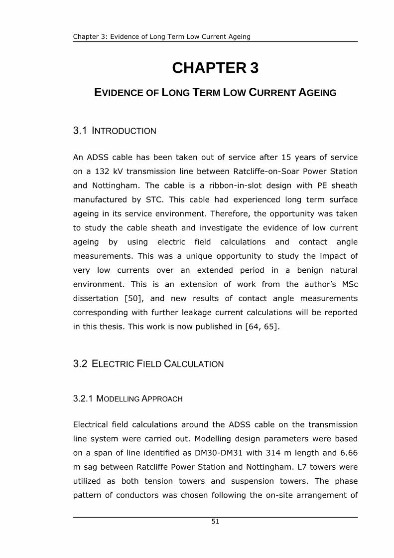
Chapter 3: Evidence of Long Term Low Current Ageing
51
3CHAPTER 3
EVIDENCE OF LONG TERM LOW CURRENT AGEING
3.1 INTRODUCTION
An ADSS cable has been taken out of service after 15 years of service
on a 132 kV transmission line between Ratcliffe-on-Soar Power Station
and Nottingham. The cable is a ribbon-in-slot design with PE sheath
manufactured by STC. This cable had experienced long term surface
ageing in its service environment. Therefore, the opportunity was taken
to study the cable sheath and investigate the evidence of low current
ageing by using electric field calculations and contact angle
measurements. This was a unique opportunity to study the impact of
very low currents over an extended period in a benign natural
environment. This is an extension of work from the author’s MSc
dissertation [50], and new results of contact angle measurements
corresponding with further leakage current calculations will be reported
in this thesis. This work is now published in [64, 65].
3.2 ELECTRIC FIELD CALCULATION
3.2.1 MODELLING APPROACH
Electrical field calculations around the ADSS cable on the transmission
line system were carried out. Modelling design parameters were based
on a span of line identified as DM30-DM31 with 314 m length and 6.66
m sag between Ratcliffe Power Station and Nottingham. L7 towers were
utilized as both tension towers and suspension towers. The phase
pattern of conductors was chosen following the on-site arrangement of

Chapter 3: Evidence of Long Term Low Current Ageing
52
ABC CBA. The sag of ADSS cable was chosen as a typical value of 1.57
m, which is 0.5 percent of the span length.
The modelling of electric fields with the specified transmission line
parameters above was built in the commercial package CDEGS and in
particular the sub package HIFREQ, with assistance by Dr. Konstantinos
Kopsidas. The results are displayed as follows.
3.2.2 MODELLING RESULTS
As discussed previously in part 1.1.2, the relative position of ADSS cable
between the 6 phase conductors may vary along the line span.
Therefore, the electric field distribution around cable can be different
along the cable length. Figure 3-1 a), b) and c) demonstrate the space
voltage potentials of electrical fields for the region near the tension
tower, mid-span and the suspension tower respectively. In the case of
the tension tower, the ADSS cable is located within the blue contour
where the induced voltage is less than 1% of single phase transmission
voltage, while for the mid-span, the ADSS cable is located between the
red and blue area with an induced voltage 1%-2% of transmission
phase voltage. Around the suspension tower, the ADSS cable is located
again in the blue area with induced voltage less than 1% of transmission
phase voltage. The simulated voltages on cable surface for these three
locations are summarized in Table 3-1.
Table 3-1: Modelling parameter Ia for different levels of stable dry-band arcs Tension Tower Mid-span Suspension Tower
Induced Voltage 0.23 kV 3.94 kV 0.22 kV
From Table 3-1, the ADSS cable is considered to be installed in a
suitable location where the induced voltage is no more than 2% of
transmission voltage along its span length. At such low voltages

Chapter 3: Evidence of Long Term Low Current Ageing
53
together with cable surface insulation resistance associated with a rural
environment, no ageing associated with discharges would be expected
[42].
Figure 3-1: The parameters of L7 tower for electric field calculation (132kV)
a) Electrical field in tension tower
a)
b) c)
c) Electrical field in mid-span
b) Electrical field in suspension tower

Chapter 3: Evidence of Long Term Low Current Ageing
54
The electric field leads to a voltage gradient along the ADSS cable, and
ultimately drives a leakage current flowing on the cable surface. Figure
3-2 shows the calculated leakage currents along the span between two
specific towers DM30-DM31 with different levels of cable surface
resistance. The current has relatively high values at the towers and in
the midway of two half spans, but returns to zero near the span centre.
Besides, this current is asymmetric from the span midpoint due to the
different cable arrangement technology between tension and suspension
towers as discussed previously. For all the three cable resistivity cases
considered, the maximum available leakage currents are lower than
0.15 mA for the entire span length, which are normally considered
insufficient for the formation of dry-band arcs [42].
Figure 3-2: Current magnitudes along the DM27-DM28 ADSS cable span [65]
3.3 VISUAL OBSERVATION FROM RECOVERED CABLE
Visual examination was conducted on the cable surface with the
observation of glossy finish lost comparing with its virgin conditions.
However, the cable sheath was still in good condition with no evidence
of electrical discharge damage at any location. Therefore, the only
possible ageing sources would be expected as UV radiation and low
0
0.05
0.1
0.15
0.2
0.25
0.3
0.35
0.4
0.45
0.5
0 62.8 125.6 188.4 251.2 314
DM30-DM31(m)
Cur
rent
(mA)
0.5MΩ/m current1MΩ/m current2MΩ/m current
Tension Tower Suspension Tower

Chapter 3: Evidence of Long Term Low Current Ageing
55
surface leakage current. Figure 3-3 shows two image examples of cable
segments.
a) cable shows no major surface damage b) cable deposits with some paint
Figure 3-3: Example of visual inspected cable segments
3.4 CONTACT ANGLE MEASUREMENT
Contact angle measurement is a method to inspect the material surface
conditions. Generally two states are defined: hydrophilic and
hydrophobic. Water on hydrophilic surfaces of materials will give a
relative lower contact angle, while water on hydrophobic material
surfaces will perform a relative higher contact angle [65].
The contact angle measurement here was conducted by dripping a
volume of 40 μl droplet onto the cable surface. A high definition image
was taken and imported in software (Vistametrix) to calculate the
relative contact angle. The measurement was carried out on the whole
cable span of DM30-DM31. The first measurement was conducted twice
for each cable location, and average value for the same location was
evaluated. As a result, 106 points of data were obtained and further
reduced to 40 points by combining the data from neighboring locations
of the same region. The second measurement was carried out on a 5
meters’ unused cable which had been exposed to natural sunlight in a
drum yard for 15 years. The third measurement was conducted on
artificially aged cable which was severely damaged by dry-band arcing
in salt-fog chamber. This later cable was not manufactured at the same

Chapter 3: Evidence of Long Term Low Current Ageing
56
time as the other two samples but had the same standard polyethylene
sheath. The results from first, second and third measurements are
summarized in Figure 3-4.
Figure 3-4: Contact angle results from a) whole cable span DM30-DM31, b)
only UV aged cable, and c) only discharge aged cable [65]
According to Figure 3-4, the average values from the only UV aged cable
and electrically aged cable are respectively upper and lower bounds
throughout the whole test results. The span of DM30-DM31, which was
aged both by UV radiation and variable low current, reflects the different
contact angles along its span length. These results show that the UV-
only ageing leads to the minimum cable surface degradation, while the
discharge ageing makes the worst surface damage to the cable. The
service-aged cable span (DM30-DM31) received more degradation than
only UV aged cable, but less damage than the cable with relatively
short-term high current. The average contact angle for the virgin cable
without any forms of ageing was measured as 98.4°, which holds the
highest value as expected.
0
10
20
30
40
50
60
70
80
90
0 62.8 125.6 188.4 251.2 314
DM30-DM31(m)
Con
tact
Ang
le(D
eg)
DM30-DM31UV agedElectrical aged
Tension Tower Suspension Tower

Chapter 3: Evidence of Long Term Low Current Ageing
57
3.5 CORRELATION OF CONTACT ANGLE AND CURRENT WITHIN A SPAN
The measured contact angle and simulated leakage current within the
span DM30-DM31 are displayed together in Figure 3-5. The result shows
that the leakage current magnitude has strong correlation with the
contact angle within the span. Generally the current peaks are
corresponding to the minimum values in contact angle. For low current
locations, the relative contact angles have high values which indicate
lower degradation. The extreme case occurs near the mid-span where
contact angle peaks while the current stays lowest.
Figure 3-5: Correlation of contact angle and current in DM30-DM31 [65]
Figure 3-6 shows the trend line between the predicted leakage currents
and measured contact angles. The contact angle decreases following the
rise of leakage current as expected. The currents used for correlation
are those for the surface conductivity of 0.5 MΩ/m as an example. In
fact the surface conductivity is not uniform and constant throughout the
cables service life, due to the complex environmental conditions. This
correlation reveals that the loss in hydrophobicity on cable surface over
the 15 years is approximately dependant on the magnitude of the local
low leakage current.
0
0.05
0.1
0.15
0.2
0.25
0.3
0.35
0.4
0.45
0.5
0 62.8 125.6 188.4 251.2 314
DM30-DM31(m)
Cur
rent
(mA
)
25
31
37
43
49
55
61
67
73
79
85
Con
tact
Ang
le (D
eg)
0.5Mohm current1Mohm current2Mohm currentDM30-DM31UV agedElectrical aged
Tension Tower Suspension Tower

Chapter 3: Evidence of Long Term Low Current Ageing
58
Figure 3-6: The trend line of contact angle against leakage current
50
55
60
65
70
75
80
0 0.02 0.04 0.06 0.08 0.1 0.12 0.14
Current(mA)
Con
tact
Ang
le(D
eg)
Measured PointLinear (Measured Point)

Chapter 3: Evidence of Long Term Low Current Ageing
59
3.6 SUMMARY
A series of investigations have been conducted on an ADSS cable after
15 years service in a benign environment looking for the evidence of
long-term low current ageing.
Electrical field calculations show that these ADSS cables have been
installed in suitable locations on the towers. Induced voltages on the
cable surface are 1% of the line voltage. Calculations show that currents
expected in this rural location are lower than those associated with
damaging arcing (a few mA is required) with no more than 0.15 mA
predicted on the sheath surface. Therefore, only low current ageing
effects could be present through its service history.
Visual inspection shows the cable surface remains in a good condition as
expected, with no major damage by the electrical discharge activities.
Water droplet contact angle measurements reveal that the cable sheath
has lost hydrophobicity due to natural UV radiation and long-term low
surface current. UV irradiation from sunlight leads to ageing of the cable
sheath. In addition the electrical current ageing contributes to ageing
within a span. Some points along the cable near towers and midway in
the two half spans perform a relatively lower hydrophobicity. This is the
first time this has been recorded, and is an important result for cables
and insulators in more aggressive installation conditions.
The correlation of contact angle and current with a span verifies that
long-term low surface currents below 0.15 mA are a factor contributing
to the ageing of cable surface properties, even if the conditions are such
that dry-band arcing does not occur. This is the first such observation.
However, ageing is not severe enough to be seen by any means other
than hydrophobicity measurement.

Chapter 4: Low Current Arc Compression
60
4CHAPTER 4
LOW CURRENT ARC COMPRESSION
4.1 THE ARC COMPRESSION PHENOMENON
Although a dry-band arc can extend to produce flashover under certain
conditions, it is usually self-limiting when several milliamperes of low
current are drawn [2]. Dry-band arcing is therefore generally considered
as a long term ageing mechanism on insulation surfaces, illustrated in
Figure 4-1 a). However, of particular concern is that in cases where the
dry-band arc is compressed in length as demonstrated in Figure 4-1 b),
the arc energy and correlated energy density will increase dramatically,
which may accelerate the long-term ageing effect into a short-term
hazard. This compression is a complicated phenomenon which may be
caused by a variety of reasons in a real power system, and may be a
rare event. However, a hypothesis of this thesis is that: even though
these compressions only occur a limited number of times over the whole
insulator service history, they may lead to the composite insulator failing
much quicker than an insulator aged under normal dry-band arcing
conditions.
a) Normal growth dry-band arc on insulation surface
b) Dry-band arc compression in length
Figure 4-1: Typical dry-band arc on insulating surface with moisture

Chapter 4: Low Current Arc Compression
61
4.2 ARC COMPRESSION SITUATIONS
On outdoor transmission line systems, low current arcing on the
insulation material surfaces is subject to complex environmental and
electrical factors. Some situations may cause the arc to compress in
length. The specified situations are respectively studied as follows:
4.2.1 ARC COMPRESSION ON INCLINED SURFACE WITH WATER FILM
The first situation describes arcing activity occurring on an inclined or
even vertical insulation surface, shown in Figure 4-2.
Figure 4-2: Dry-band arc compression on inclined surface between water
films
In Figure 4-2 a), thermal and moisture balances have been reached
allowing formation of a stable dry-band arc with relative constant
maximum arc length and repeatable electrical behaviour. When the
sample is inclined as in Figure 4-2 b), the upper water film and lower
water film, whose edges are at the dry-band boundaries, will tend to
move down the insulator core due to gravity. The upper film tends to
move faster because of moisture feeding from the rod above it and
because of the breakdown of surface tension due to the arc. The dry-
band gradually moves down the rod by this means until the lower water
film is replaced by the immobile metallic fitting. The metallic fitting then
becomes an immovable lower edge of the dry-band. In the meantime,
the upper water film can still move downwards. Following this, a single

Chapter 4: Low Current Arc Compression
62
stable dry-band arc remains but the arc length is physically reduced in
length. The length of the arc is reduced to extinction unless a new
balance is achieved.
For the transmission line elements, the possible situations for realizing
dry-band arc compression in this situation are either arcing on the
tensioned ADSS cable attaching to tower shown in Figure 4-3 a), or
arcing on the suspension insulators with inclined surface shown in Figure
4-3 b).
Figure 4-3: Inclined surface for arc compression on power transmission lines
4.2.2 ARC COMPRESSION UNDER WIND AND RAIN ENVIRONMENT
Figure 4-4 shows another possible situation for arc compression on
insulation surface with wind and rain. As shown in Figure 4-4 a), with
the wet deposition and induced leakage current flowing on the insulation
surface, the dry-band arc could ignite and grow to the maximum length
achieving the dynamic balance between the dry-band expansion by
Joule heating effect and dry-band extinction by continuous water
deposition. The effect of wind in the horizontal position, shown in Figure
4-4 b), is that the right-hand water film which is close to the wind
source could be blown into the dry-band. In the meantime, the left-hand
water film receives weaker wind but also starts moving towards the left.
During this stage, the arcing could possibly continue striking so that the
b) Arcing compression on inclined insulator surface
a) Arcing compression on inclined ADSS cable surface

Chapter 4: Low Current Arc Compression
63
whole dry-band area would move till the left part of water film firstly
reaches the metallic fitting or cable joint and becomes stationary. In the
meantime, the right-hand water film still moves leftwards. As the result,
the dry-band arc is physically compressed in this situation.
Figure 4-4: Dry band arc compression under wet rain and wind conditions
The following Chapter 5 of the Thesis Experimental Part will conduct the
relevant tests base on the two proposed arcing compression situations
above.

Chapter 5: Experimental
64
5CHAPTER 5
EXPERIMENTAL
5.1 TESTING IN A FOG ENVIRONMENT
5.1.1 INTRODUCTION The wet outdoor conditions around the insulator surface are of
importance for electrical discharge growth, and one of the most common
environmental factors affecting overhead line elements is fog. The inland
areas may expose insulators to clean-fog, while the offshore or
contaminated environments may involve the salt-fog. The experimental
study in this chapter will be conducted to investigate the fog
environment for the electrical discharge formation and growth, following
the testing standards in accordance with IEC 61109. Here the dry-band
arcing phenomenon in both clean-fog environments and salt-fog
environments are compared. The discussion will focus on the electrical
properties of arcs under the different fog conditions. The most severe
environment will be identified as the basis for the further experimental
studies in this thesis.
5.1.2 TEST ARRANGEMENT
Figure 5-1 demonstrates the arrangement of testing in a fog
environment. The transformer provides single-phase AC voltage up to
42 kV at its secondary side. A current limiting resistor is used to limit
the leakage current to less than 10 mA. A fibre-glass reinforced rod
which is sheathed in silicone rubber insulation compound is used as the
test sample. This structure represents a typical composite insulator core
without sheds to simplify the test. The sample is suspended into the fog

Chapter 5: Experimental
65
environmental chamber with the high voltage end connected to the
transformer secondary via the current limiting resistor, and the low
voltage end is attached to the earthed frame via a 1 kΩ current
measuring resistor. The connection points between the test circuit and
sample are on electrodes, which are formed by wrapping copper strip
tightly around the two ends of rod.
Transformer Secondary
Current limit resistor
Current signal
Die
lect
ric ro
pe
FOG CHAMBER
Salt-fog environment
Vol
tage
div
ider
Voltage signal
Nozzle
Nozzle
LABVIEW DATA ACQUISITION SYSTEM
Nozzle Nozzle
Nozzle Nozzle
Nozzle
Nozzle
Arcing
Test sample
NozzleWater pipeline
Air pipeline
0-42 kV
Figure 5-1: Test arrangement of Testing in a Fog Environment
The fog environmental chamber is a sealed and waterproof chamber
with a total volume of 16.8 m3. A 125 cm X 90 cm glass window allows
visual observation of the experiment by the chamber operator although
a full fog is in operation. Six nozzles are placed around the internal wall
of chamber. An air pipeline and a water pipeline are introduced into the
chamber and mixed together in the nozzles. Air is supplied from an air
compressor with the maximum output of 100 psi. Water is pumped from
a 220 litre tank filled with the solution which is either tap-water, de-
ionized water or salt water depending on the test specification. The
water is sprayed to a fog by the compressed air in the nozzles. The salt
fog tests are in accordance with IEC 61109 (1992).

Chapter 5: Experimental
66
The control of the fog environmental chamber includes the fog
precipitation rate control and voltage control. The air pressure regulator
and pump valve are used to control the fog injection. As the required
precipitation rate is 6.7 ± 1.7 l/hr, the air pressure regulator is set to 1
bar. Prior to running a test, the chamber precipitation rate can be
verified using a 15 cm diameter petri dish on the chamber floor
collecting 17.5±4.4 g of water per hour. Voltage control is achieved by
the Labview system outside the chamber to control a motor running
clockwise or anticlockwise to step up or down the rheostat feeding the
transformer. A series of interlocks and trip switches such as door
interlock, over current trip switch, timer relay switch and key interlock
switch are attached to the chamber for the safety and security purposes.
The data measurement and acquisition system consists of a 10,000:1
voltage divider which is used to pick up the voltage across the sample.
The 1 kΩ current measurement resistor is used to acquire the leakage
current flowing on sample surface. Both voltage and current signals are
recorded by a National Instrument Labview system. A video camera is
used to capture the electrical discharges videos and images for the test
record and arc length measurement purposes.
5.1.3 TEST PROCEDURE Three groups of tests are conducted in the fog environment as follows,
5.1.3.1 ARC FORMATION TEST This test aims to study the dry-band arc formation process from dry
surface to wet surface until the arc ionization. The electrical properties
in terms of voltage, current and their phase relationship are investigated
during the test. Clean-fog produced by tap water (with conductivity of
600 μs/cm) is used in this test as the arcing phenomenon in the clean-

Chapter 5: Experimental
67
fog environment is gentle and gradual, which is relatively easy to
capture.
I. Transformer voltage is fixed to 30 kV (RMS). The current limit resistor
is chosen as 2 MΩ throughout the test.
II. The sample surface is uniformly roughened with abrasive paper to
reduce its surface hydrophobicity for the ease of fog adhesion on the
sample.
III. Initially before the fog injection, the sample surface needs to be
dried throughout. After applying the source voltage, the fog is
immediately switched on to produce the clean-fog with precipitation rate
of 6.7 l/hr.
IV. By the continuous fog deposition together with the high voltage
gradient across the sample, the dry-band arcing will eventually form on
the surface. The arc voltage, current and arcing image are recorded for
the whole process from surface getting wet to the arc formation.
5.1.3.2 ARC GROWTH TEST The arc growth test is to investigate the process of free growth of arcs in
the salt-fog environment. Arcs for different voltage and current levels
with variable arc lengths are produced by the test with the following
procedure:
I. The salt-fog is prepared and generated from salt mixed with water to
a conductivity of 16,000 μs/cm.
II. The transformer voltage is fixed to approximately 10 kV (RMS) with a
current limiting resistor to 8 MΩ, in order to get a long sustained, stable
arc with 1.5 mA (peak) arcing current. In this way a balance is achieved

Chapter 5: Experimental
68
between arc expansion by Joule heating and arc extinction by fog
deposition.
III. After 30 minutes, gradually increase the transformer voltage to
obtain a 2.0 mA (peak) arc. The arc expands in length due to enhanced
Joule heating. Wait for another 30 minutes until a new equilibrium is
achieved.
IV. Keep increasing the transformer voltage to get 2.5 mA, 3.0 mA, 3.5
mA and 4.0 mA arcs, with 30 minute intervals between each level for
the stable arc formation with respectively new balance.
V. Arcing voltage, current and arc lengths are recorded by the Labview
for the further analysis.
5.1.3.3 FOG COMPARISON TEST The arcing behaviour in both clean-fog and salt-fog surroundings are
compared, in order to investigate the different discharge properties in
variable environments, and to identify the most severe conditions for
dry-band arcing growth. The test procedures are as follows:
I. Fill the water tank with tap water to create clean-fog environment
around the sample.
II. Switch on the transformer, vary the voltage output (from 10 kV to 30
kV) to get stable arcs for different levels.
III. Clean the sample surface, refill the water tank with salt mixed water
to reach a conductivity of 16,000 μs/cm. Generate salt-fog environment.
IV. Vary the voltage output (from 10 kV to 30 kV) to obtain the dry-
band arcs for different levels corresponding to procedure II.

Chapter 5: Experimental
69
V. The voltage, current and arcing images are stored in the Labview
data acquisition system. Further analysis is conducted based on the
comparison of arcing phenomenon between clean-fog and salt-fog
environment.
5.1.4 TEST RESULTS 5.1.4.1 ARC FORMATION TEST
For the dry-band arc initial formation, there are 5 stages identified as:
STAGE 1
At the beginning when the sample surface is still dry, the leakage
current presents a peak value of 14 μA, which is low due to the excellent
dielectric properties of silicone rubber. In the meantime, the current
leads the voltage to approximately 90°, showing a capacitive
characteristic and minimal resistive current on the sample. Figure 5-2 a)
shows the measured voltage and current traces during this stage.
STAGE 2
After the sample surface has become wet due to the fog deposition, the
surface impedance reduces and the leakage current begins to grow. In
the meantime, the trace of leakage current gradually becomes inphase
with the voltage, shifting from a capacitive to resistive nature. Figure
5-2 b) and c) show the phase and magnitude change of leakage current
within 3 minutes after the fog injection.
STAGE 3
The current and voltage traces are ultimately in phase after 220 seconds
from the test start in Figure 5-2 d), and the magnitude of leakage
current significantly increases to 156 μA, which is 11 times higher than

Chapter 5: Experimental
70
the current at stage 1. Figure 5-3 summarizes the trend of current
increasing and phase shifting from stage 1 to stage 3. The current
increase is due to the continuous moisture formation which significantly
reduces the surface resistance of sample and allows higher leakage
current. The phase shift results from the transformation of sample
surface property from capacitive (dry silicone rubber) to resistive (wet
moisture).
STAGE 4
As the sample surface continues to become wetter forming a thicker
layer of clean-fog deposition, the leakage current begins to distort after
470 seconds of test as shown in Figure 5-2 e). Low current discharges
are present along with the current distortion, which increases with the
rise of leakage current from 0.4 mA to 1.2 mA (peak) shown in Figure
5-2 f) and g).
STAGE 5
As the leakage current increases to above 1 mA, dry-band arcs occur.
Initially there are several unstable arcs striking on the sample surface,
but finally becomes one single arc shown in Figure 5-4. After
approximate 48 minutes of the test running, the dry-band arc becomes
stable with relatively constant length and repeatable voltage and current
profiles for every power cycle shown in Figure 5-2 h).

Chapter 5: Experimental
71
The current scale in a), b), c) and d) is ±200 μA; the current scale in e), f)
and g) is 2 mA; the current scale in h) is 4 mA
Figure 5-2: Voltage and current curves from stage 1 to stage 5 in the clean-fog environment
-50
-40
-30
-20
-10
0
10
20
30
40
50
0 5 10 15 20 25 30 35 40
Time (ms)
Volta
ge (k
V)
-200
-160
-120
-80
-40
0
40
80
120
160
200
Cur
rent
(uA)
VoltageCurrent
Test beginning-50
-40
-30
-20
-10
0
10
20
30
40
50
0 5 10 15 20 25 30 35 40
Time (ms)
Volta
ge (k
V)
-200
-160
-120
-80
-40
0
40
80
120
160
200
Cur
rent
(uA)
VoltageCurrent
90 Seconds Later
a) b)
Stage 1 Stage 2
-50
-40
-30
-20
-10
0
10
20
30
40
50
0 5 10 15 20 25 30 35 40
Time (ms)
Volta
ge (k
V)
-2
-1.6
-1.2
-0.8
-0.4
0
0.4
0.8
1.2
1.6
2
Cur
rent
(mA)
VoltageCurrent
2800 Seconds Later-50
-40
-30
-20
-10
0
10
20
30
40
50
0 5 10 15 20 25 30 35 40
Time (ms)
Volta
ge (k
V)
-4
-3.2
-2.4
-1.6
-0.8
0
0.8
1.6
2.4
3.2
4
Cur
rent
(mA
)
VoltageCurrent
3 hours Later
g) h)
Stage 4 Stage 5
-50
-40
-30
-20
-10
0
10
20
30
40
50
0 5 10 15 20 25 30 35 40
Time (ms)
Vol
tage
(kV
)
-200
-160
-120
-80
-40
0
40
80
120
160
200
Cur
rent
(uA
)
VoltageCurrent
150 Seconds Later-50
-40
-30
-20
-10
0
10
20
30
40
50
0 5 10 15 20 25 30 35 40
Time (ms)
Vol
tage
(kV
)
-200
-160
-120
-80
-40
0
40
80
120
160
200
Cur
rent
(uA
)
VoltageCurrent
220 Seconds Later
c) d)
-50
-40
-30
-20
-10
0
10
20
30
40
50
0 5 10 15 20 25 30 35 40
Time (ms)
Vol
tage
(kV
)
-2
-1.6
-1.2
-0.8
-0.4
0
0.4
0.8
1.2
1.6
2
Cur
rent
(mA
)
VoltageCurrent
470 Seconds Later-50
-40
-30
-20
-10
0
10
20
30
40
50
0 5 10 15 20 25 30 35 40
Time (ms)
Vol
tage
(kV
)
-2
-1.6
-1.2
-0.8
-0.4
0
0.4
0.8
1.2
1.6
2
Cur
rent
(mA
)
VoltageCurrent
1234 Seconds Later
e) f)
Stage 2 Stage 3
Stage 4 Stage 4

Chapter 5: Experimental
72
0
18
36
54
72
90
0 44 88 132 176 220Experiment Time (Sec)
Pha
se S
hift
(Deg
)
0
40
80
120
160
200
Cur
rent
(uA
)
Phase shiftPeak current
Figure 5-3: Summary of phase shift and current increase from stage 1 to
stage 3 in the clean-fog environment
Figure 5-4: The transformation from several arcs to one single arc
5.1.4.2 ARC GROWTH TEST
Figure 5-5 shows the current and voltage profiles and corresponding arc
lengths for different current levels of 1.5 mA, 2.0 mA, 2.5 mA, 3.0 mA,
3.5 mA and 4.0 mA in the salt-fog conditions specified in Part 5.1.3.2.
Each test was conducted for at least 30 minutes to allow equilibrium to
be achieved between arc expansion by joule heating and arc reduction
by fog deposition. Although the instantaneous arcing current is changing
with dynamic arcs in each angle, the dry-band length becomes constant
following the establishment of equilibrium. Therefore, fairly constant arc
lengths were measured in each case. The results show the dry-band arc
grows in physical length when the arc current increases. The visible arc
also becomes thicker and brighter for higher current levels. Detailed

Chapter 5: Experimental
73
discussion based on these results will be presented in the following part
5.1.5.2 (Results Analysis).
a) Dry-band arcing with 1.5 mA current (peak)
b) Dry-band arcing with 2.0 mA current (peak)
c) Dry-band arcing with 2.5 mA current (peak)
-50
-40
-30
-20
-10
0
10
20
30
40
50
0 5 10 15 20 25 30 35 40
Time (ms)
Vol
tage
(kV
)
-5
-4
-3
-2
-1
0
1
2
3
4
5
Cur
rent
(mA
)
VoltageCurrent
-50
-40
-30
-20
-10
0
10
20
30
40
50
0 5 10 15 20 25 30 35 40
Time (ms)
Volta
ge (k
V)
-5
-4
-3
-2
-1
0
1
2
3
4
5
Cur
rent
(mA
)
VoltageCurrent
-50
-40
-30
-20
-10
0
10
20
30
40
50
0 5 10 15 20 25 30 35 40
Time (ms)
Vol
tage
(kV
)
-5
-4
-3
-2
-1
0
1
2
3
4
5
Cur
rent
(mA
)
VoltageCurrent

Chapter 5: Experimental
74
d) Dry-band arcing with 3.0 mA current (peak)
e) Dry-band arcing with 3.5 mA current (peak)
f) Dry-band arcing with 4.0 mA current (peak)
Figure 5-5: Dry-band arcs for different current levels from 1.5 mA to 4.0 mA
in salt-fog environment (Left figure shows electrical properties of discharge) (Right image shows the discharge physical length)
-50
-40
-30
-20
-10
0
10
20
30
40
50
0 5 10 15 20 25 30 35 40
Time (ms)
Vol
tage
(kV)
-5
-4
-3
-2
-1
0
1
2
3
4
5
Cur
rent
(mA)
VoltageCurrent
-50
-40
-30
-20
-10
0
10
20
30
40
50
0 5 10 15 20 25 30 35 40
Time (ms)
Vol
tage
(kV
)
-5
-4
-3
-2
-1
0
1
2
3
4
5
Cur
rent
(mA
)
VoltageCurrent
-50
-40
-30
-20
-10
0
10
20
30
40
50
0 5 10 15 20 25 30 35 40
Time (ms)
Vol
tage
(kV
)
-5
-4
-3
-2
-1
0
1
2
3
4
5
Cur
rent
(mA
)
VoltageCurrent

Chapter 5: Experimental
75
5.1.4.3 FOG COMPARISON TEST
Figure 5-6 shows an example of arc images in both clean-fog and salt-
Testing in a Fog Environments. Under the clean-fog condition, the arc
burns with a blue colour. But in case of the salt-fog environment Figure
5-6 b), the arc flame appears yellow. This is due to the presence of
sodium ion (Na+) from salt-fog surroundings during the arcing period.
Sodium makes the flame yellow and its spectrum tends to dominate
over others.
a) Dry-band arc in clean-fog b) Dry-band arc in salt-fog
Figure 5-6: Arc images in both clean-fog and salt-fog environment
Figure 5-7 shows an example of dry-band arc behaviours in respective
clean-fog and salt-fog environment. The further discussion will be
conducted in part 5.1.5.3.
-50
-40
-30
-20
-10
0
10
20
30
40
50
0 5 10 15 20 25 30 35 40 45
Time (ms)
Vol
tage
(kV
)
-5
-4
-3
-2
-1
0
1
2
3
4
5
Cur
rent
(mA
)
VoltageCurrent
Clean-fog Environment Salt-fog Environment
0 5 10 15 20 0 5 10 15 20
Figure 5-7: Voltage and current behaviours for arcs in different fog
environments

Chapter 5: Experimental
76
5.1.5 RESULTS ANALYSIS
5.1.5.1 CHANGE OF MATERIAL SURFACE PROPERTY IN FOG ENVIRONMENT
From stage one to stage three in the results of the initial formation test
(Figure 5-3, part 5.1.4.1), the voltage and current traces were 90
degrees out of phase, and gradually became in phase after 220 seconds
of clean-fog injection. A simplified electrical model is used to analyze the
change of surface property in Figure 5-8. The sample surface is
represented by a capacitor parallel with a variable resistor. At the test
beginning when the sample surface is still dry without fog injection, the
variable resistor taps at point ‘a’ with an extremely high value. The
majority of leakage current is flowing in the capacitor path given an
initial dry current of 14 μA corresponding to the capacitance calculated
around 1 pF, so that the capacitive property dominates the whole
electrical characteristics of sample surface. From experimental
observation, the current leads the voltage at this stage.
Figure 5-8: Electrical model of silicone rubber sample surface
When the sample becomes wet due to the fog deposition, the value of
resistor drops dramatically, to the lowest value which is equivalent to
the surface fog deposition resistance (around 6 MΩ for the clean fog
case), but the capacitive part of circuit does not change. So the leakage
current increases in the resistive branch, which changes the electrical
characteristic of sample surface to be resistive of 10 MΩ (6 MΩ wet
surface resistance and 4 MΩ arcing resistance). This is the reason why

Chapter 5: Experimental
77
the leakage current is finally in phase with test voltage after the sample
surface being fully wetted.
5.1.5.2 COMPARISON BETWEEN ARCS WITH DIFFERENT CURRENT LEVELS
BREAKDOWN VOLTAGE AND ARC VOLTAGE
Figure 5-9 shows one cycle of typical voltage and current traces for 1.5
mA (peak) dry-band arcing. From A to B, the arc current stays at zero
because of the high impedance of dry-band area. When the supply
voltage reaches a certain value, the arc starts striking across the dry-
band with the significant increase of arcing current. The breakdown
voltage is defined as the threshold voltage for dry-band arc ignition.
During the arcing period from B to C, the arc voltage is determined by:
su ( ) v - ( ) ( )= × − ×a a resistor a moisturet i t R i t R 5-1
Where: ua(t) is the arc voltage, ia(t) is the arc current, vs is the
instantaneous open-circuit transformer voltage, Rresistor is the current
limiting resistor and Rmoisture is the total resistance of water layer.
-20
-16
-12
-8
-4
0
4
8
12
16
20
0 5 10 15 20
Time (ms)
Volta
ge (k
V)
-2
-1
0
1
2
Cur
rent
(mA
)
VoltageCurrent
A B C
Breakdown voltage
Arcing period
B'
Before arcing
After arcing
Figure 5-9: Identification of arcing period and breakdown voltage of 1.5 mA
arc

Chapter 5: Experimental
78
In the salt-fog conditions, experimental work shows that the resistance
of water layer (Rmoisture) is approximately 0.85 kΩ (at room temperature)
for the sample length of 30 cm. For all cases of arc current below 4 mA,
the voltage drop across the water layer (ia(t) x Rmoisture) is less than
0.02% of the arc voltage (ua(t)) and in this analysis is neglected. So the
measured voltage signal at the point of voltage divider in Figure 5-1 is
approximately the arc voltage (ua(t)), and the relationship between arc
voltage and arc current can be simplified as:
su ( ) - ( )= ×a a resistort v i t R 5-2
Figure 5-10 shows the relationship between the breakdown voltage,
source voltage (peak) and arc length. Labels of 1.5 mA, 2.0 mA … 4.0
mA represent the arcs with the peak current from 1.5 mA to 4.0 mA
respectively. The shorter dry-band length is corresponding to the lower
breakdown voltage. If the arc current increases, the enhanced joule
heating effect will expand the dry-band area, and therefore, requires
higher voltage to breakdown the air gap. The result shows a linear
relationship in the range of 1.8 cm to 7.1 cm length of arcs with 15.8 kV
to 37.4 kV breakdown voltages.
0
10
20
30
40
50
1 2 3 4 5 6 7 8Arc length (cm)
Bre
akdo
wn
& S
ourc
e V
olta
ge (k
V)
Breakdown VoltageSource Voltage PeakLinear (Breakdown Voltage)Linear (Source Voltage Peak)
(1.5mA)
(2.0mA)(2.5mA)
(3.0mA)
(3.5mA) (4.0mA)
Figure 5-10: The relationship between breakdown voltage, source voltage
peak and arc length

Chapter 5: Experimental
79
ARCING PERIOD
Figure 5-11 summaries the arcing period against arc length for the dry-
band arcs from 1.5 mA to 4.0 mA (peak) in the salt-fog environment. As
arc current increases, the arcing period shows slight reduction but no
significant change. The arcing period is determined by the arc ignition
time at point B and arc extinction time at point C as marked in Figure
5-9. As discussed in the previous section of ‘breakdown voltage and arc
voltage’, the arcing breakdown voltage increases linearly corresponding
to the arc length expansion. The arc ignition time is fairly constant for
different arcs shown in Figure 5-5. Further, the arc extinction time does
not dramatically change for each case. Therefore, the arcing period
reduces only 11.5% for an increase of arc length from 1.83 to 7.07 cm
at different current levels.
y = -0.1172x + 6.1652R2 = 0.6004
0
1
2
3
4
5
6
7
8
9
10
1 2 3 4 5 6 7 8Arc length (cm)
Arci
ng p
erio
d (m
s)
(1.5mA)(2.0mA)
(2.5mA)(3.0mA) (3.5mA) (4.0mA)
Figure 5-11: The relationship between arcing period and arc length
V-I CHARACTERISTICS
V-I (voltage against current) characteristics for dry-band arcs with
different current levels show non-linear relationship between arcing
voltage and current in Figure 5-12. For each individual current level, V-I
curve with symmetrical two parts are observed in both positive and
negative coordinates domain. The rough geometry of V-I curve appears
a triangle shape, with point B (B′ in negative half cycle) representing an
arc ignition, point C (C′ in negative half cycle) representing a peak

Chapter 5: Experimental
80
current arc and point A (A′ in negative half cycle) representing an arc
extinction, as demonstrated in an example of 4.0 mA arc. The line AB
shows the V-I characteristic in the pre-arcing period, while line BC
shows the change of V-I when the arc starts striking. The line CA
represents the V-I curve during the arcing period, while line A to point
(0,0) shows the V-I behaviour in the post-arcing period. Following the
rise of transformer source voltage, both arcing voltage and current will
be increased, corresponding to the larger triangle area from 1.5 mA to
4.0 mA dry-band arcs.
-40
-30
-20
-10
0
10
20
30
40
-5 -4 -3 -2 -1 0 1 2 3 4 5
Current (mA)
Vol
tage
(kV
)
1.5 mA arc2.0 mA arc2.5 mA arc3.0 mA arc3.5 mA arc4.0 mA arc
Figure 5-12: V-I (voltage against current) characteristics of dry-band arcs for
different current levels from 1.5 mA to 4.0 mA
ARC RESISTANCE
The instantaneous arc resistance is calculated by the ratio of arc voltage
and arc current traces measured from test:
( )( )
( )
r = a ta t
a t
ui
5-3
where ra(t) is the arc resistance, ua(t) is the measured arc voltage, ia(t) is
the measured arc current.
A
B
C
A′
B′
C′

Chapter 5: Experimental
81
Figure 5-13 shows an example of arc resistance for four half cycles of
arcing activity with 2.5 mA peak current. Arc resistance varies from 4
MΩ to 6 MΩ during the arcing period, reaching the lowest value when
the arc is fully developed with maximum arcing current. The highest arc
resistance is taken from the point when the arc starts to strike.
0
2
4
6
8
10
12
14
16
18
20
0 5 10 15 20 25 30 35 40Time (ms)
Res
ista
nce
(MΩ
)
Resistance
Figure 5-13: Instantaneous arc resistances of 2.5 mA peak current arcing for
four consecutive half power cycles
Figure 5-14 summarizes the arc resistance for different arcs from arc
growth tests in a salt-fog environment. The range of arc resistance
variation gradually decreases from 5-7 MΩ to 3.5-5 MΩ. This is due to
the faster growth rate of arcing current comparing to the arcing voltage
when the supply voltage rises from a) to f) in Figure Figure 5-5.
0
2
4
6
8
10
12
14
16
18
20
Time (ms)
Res
ista
nce
(MΩ
)
1.5mA arc 2.0mA arc 2.5mA arc 3.0mA arc 3.5mA arc 4.0mA arc0 5 10 0 5 10 0 5 10 0 5 10 0 5 10 0 5 10
Figure 5-14: Instantaneous arc resistances of arcs in different current levels

Chapter 5: Experimental
82
ARCING RESISTIVITY
Figure 5-15 shows the instantaneous resistivity of arcs in different
current levels in the salt-testing in a Fog Environment. The arc
resistivity decreases faster than resistance from 1.0 mA to 4.0 mA
because of the arc length expansion:
( )r ( ) = a
resistivitya
r ttL
5-4
Where Rresistivity(t) is the instantaneous arc resistivity. ra(t) is the arc
resistance, La is the measured arc length.
0
40
80
120
160
200
240
280
320
360
400
Time (ms)
Res
istiv
ity (M
Ω/m
)
Instantaneous resistivityMinimum resistivity trend
1.5mA arc 2.0mA arc 2.5mA arc 3.0mA arc 3.5mA arc 4.0mA arc0 5 10 0 5 10 0 5 10 0 5 10 0 5 10 0 5 10
Figure 5-15: Instantaneous arc resistivity of arcs in different current levels
5.1.5.3 COMPARISON BETWEEN CLEAN-FOG AND SALT-FOG ENVIRONMENT
The fog comparison test described in part 5.1.3.3 yields the voltage and
current traces of dry-band arcs in both clean-fog and salt-fog
environments in Figure 5-7. For the salt-fog environment, the
experimental measured voltage during the arcing period drops
significantly from 38 kV to 15 kV, but for the clean-fog environment, the
arcing voltage does not fall dramatically when the arc is burning. The
reason for the difference is that the voltage signal measured at the high
voltage sample end (in Figure 5-1) contains two parts which are arc

Chapter 5: Experimental
83
voltage and water layer voltage. As discussed from Equation 5-1 in
section 5.1.5.2 ‘Breakdown Voltage and Arc Voltage’, the water layer on
the sample surface under the salt-fog environment is highly conductive
to approximate 0.85 kΩ. Comparing to the minimum instantaneous arc
resistance of 4 MΩ previously shown in Figure 5-14, the salt-water layer
only holds less than 0.02% of arc voltage, so that can be neglected. In
contrast, the resistance of water layer in the clean-fog environment,
with the minimum possible value of 6 MΩ as discussed in section 5.1.5.1,
is much higher than in the salt-fog condition, which could take up to
60% of arc voltage. Therefore, the measured voltage in the clean-fog
consists largely of water layer voltage. From this point of view, the
voltage signal from salt-fog environment can more precisely reflect the
real arcing voltage by effectively reducing the water layer influence.
The arcing current is higher in the salt-fog environment compared to the
clean-fog under the sample supply voltage in the Figure 5-7. This is due
to the conductivity of moisture which allows more leakage current to
flow. Therefore, the salt-fog environment represents the most severe
conditions for test samples as the arcs can be fully developed on the
material surface.

Chapter 5: Experimental
84
5.2 TESTING WITH INCLINED SAMPLES
5.2.1 INTRODUCTION
As discussed previously, the salt-fog environment can be considered as
providing severe conditions for the dry-band arc growth on an insulation
material surface. On overhead transmission lines, insulators are
suspended in vertical or inclined positions which may enhance surface
moisture’s mobility because of gravity. This phenomenon, in turn, may
affect arcing properties such as physical length due to arc compression
(more detailed information is given in Chapter 4). In this section,
Testing with Inclined Samples will be conducted to further analyze the
electrical properties of compressed arcs on the insulation surface for
different slope angles in the salt-fog environment. Arc length,
breakdown voltage, arc current, arc power and arc energy will be
analyzed and conclusions are drawn that the compressed arc may have
a higher energy dissipation which could damage the material surface
more rapidly and severely than normal arcing conditions.
5.2.2 TEST ARRANGEMENT
Figure 5-16 illustrates the design of the Testing with Inclined Samples.
The test sample is a 22 mm diameter rod, consisting of 4 mm radial
thickness commercial silicone rubber which is a typical composite
insulator material on a glass-fibre reinforced core. The transformer
secondary is fixed to 17.4 kV (RMS) with a 7 MΩ current limiting resistor
to obtain 2.0 mA (peak value) arc current when the sample is in the
horizontal position. The data acquisition system and salt-fog
environmental chamber are the same as in part 5.1 of Testing in a Fog
Environment.

Chapter 5: Experimental
85
Figure 5-16: Test arrangement of Testing with Inclined Samples
A motor is introduced to control the inclination of sample. This rotation
system connects to one sample end by a dielectric string via a pulley
which is fitted on the chamber ceiling, while the other end of string is
attached to a motor. This string is made from silicone rubber which can
provide excellent dielectric properties to avoid leakage current flowing in
this path. The motor is remotely controlled by a double-way switch
outside the chamber to be rotated either clockwise or anticlockwise. The
motor speed is chosen at 1.5 rpm giving a linear string speed of 1.2
mm/s in order to make sure the lifting or falling of the sample is smooth
and gradual (approximately 20° of slope angle per minute).
The salt-fog environment is made by salt mixed with water to provide a
conductivity of 16,000 μs/cm. The air pressure of fog injection is 1.0 bar,
and the resulting precipitation rate in the chamber is approximate 0.2
l/m3.
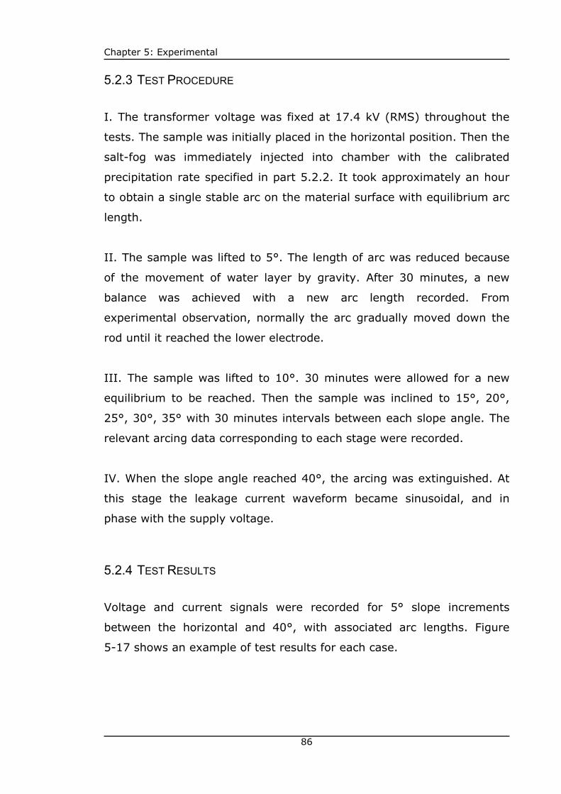
Chapter 5: Experimental
86
5.2.3 TEST PROCEDURE
I. The transformer voltage was fixed at 17.4 kV (RMS) throughout the
tests. The sample was initially placed in the horizontal position. Then the
salt-fog was immediately injected into chamber with the calibrated
precipitation rate specified in part 5.2.2. It took approximately an hour
to obtain a single stable arc on the material surface with equilibrium arc
length.
II. The sample was lifted to 5°. The length of arc was reduced because
of the movement of water layer by gravity. After 30 minutes, a new
balance was achieved with a new arc length recorded. From
experimental observation, normally the arc gradually moved down the
rod until it reached the lower electrode.
III. The sample was lifted to 10°. 30 minutes were allowed for a new
equilibrium to be reached. Then the sample was inclined to 15°, 20°,
25°, 30°, 35° with 30 minutes intervals between each slope angle. The
relevant arcing data corresponding to each stage were recorded.
IV. When the slope angle reached 40°, the arcing was extinguished. At
this stage the leakage current waveform became sinusoidal, and in
phase with the supply voltage.
5.2.4 TEST RESULTS
Voltage and current signals were recorded for 5° slope increments
between the horizontal and 40°, with associated arc lengths. Figure
5-17 shows an example of test results for each case.

Chapter 5: Experimental
87
a) Dry-band arcing in horizontal position
b) Dry-band arcing at 5° slope angle
c) Dry-band arcing at 10° slope angle
-50
-40
-30
-20
-10
0
10
20
30
40
50
0 5 10 15 20 25 30 35 40
Time (ms)
Vol
tage
(kV)
-5
-4
-3
-2
-1
0
1
2
3
4
5
Cur
rent
(mA
)
VoltageCurrent
Arcing period
Experiment resultSlope angle: 0°
Equilibrium arc length: 2.32 cm
-50
-40
-30
-20
-10
0
10
20
30
40
50
0 5 10 15 20 25 30 35 40
Time (ms)
Volta
ge (k
V)
-5
-4
-3
-2
-1
0
1
2
3
4
5
Cur
rent
(mA
)
VoltageCurrent
Experiment resultSlope angle: 5°
Equilibrium arc length: 2.28 cm
Arcing period
-50
-40
-30
-20
-10
0
10
20
30
40
50
0 5 10 15 20 25 30 35 40
Time (ms)
Vol
tage
(kV
)
-5
-4
-3
-2
-1
0
1
2
3
4
5
Cur
rent
(mA
)
VoltageCurrent
Experiment resultSlope angle: 10°
Equilibrium arc length: 2.16 cm
Arcing period

Chapter 5: Experimental
88
d) Dry-band arcing at 15° slope angle
e) Dry-band arcing at 20° slope angle
f) Dry-band arcing at 25° slope angle
-50
-40
-30
-20
-10
0
10
20
30
40
50
0 5 10 15 20 25 30 35 40
Time (ms)
Volta
ge (k
V)
-5
-4
-3
-2
-1
0
1
2
3
4
5
Cur
rent
(mA)
VoltageCurrent
Arcing period
Experiment resultSlope angle: 15°
Equilibrium arc length: 1.94 cm
-50
-40
-30
-20
-10
0
10
20
30
40
50
0 5 10 15 20 25 30 35 40
Time (ms)
Volta
ge (k
V)
-5
-4
-3
-2
-1
0
1
2
3
4
5
Cur
rent
(mA)
VoltageCurrent
Experiment resultSlope angle: 20°
Equilibrium arc length: 1.81 cm
Arcing period
-50
-40
-30
-20
-10
0
10
20
30
40
50
0 5 10 15 20 25 30 35 40
Time (ms)
Volta
ge (k
V)
-5
-4
-3
-2
-1
0
1
2
3
4
5
Cur
rent
(mA)
VoltageCurrent
Experiment resultSlope angle: 25°
Equilibrium arc length: 1.72 cm
Arcing period

Chapter 5: Experimental
89
g) Dry-band arcing at 30° slope angle
h) Dry-band arcing at 35° slope angle
i) Dry-band arcing at 37° slope angle
-50
-40
-30
-20
-10
0
10
20
30
40
50
0 5 10 15 20 25 30 35 40
Time (ms)
Vol
tage
(kV
)
-5
-4
-3
-2
-1
0
1
2
3
4
5
Cur
rent
(mA
)
VoltageCurrent
Experiment resultSlope angle: 37°
Equilibrium arc length: 0.92 cm
Arcing period
-50
-40
-30
-20
-10
0
10
20
30
40
50
0 5 10 15 20 25 30 35 40
Time (ms)
Vol
tage
(kV)
-5
-4
-3
-2
-1
0
1
2
3
4
5
Cur
rent
(mA)
VoltageCurrent
Experiment resultSlope angle: 30°
Equilibrium arc length: 1.45 cm
Arcing period
-50
-40
-30
-20
-10
0
10
20
30
40
50
0 5 10 15 20 25 30 35 40
Time (ms)
Vol
tage
(kV
)
-5
-4
-3
-2
-1
0
1
2
3
4
5
Cur
rent
(mA
)
VoltageCurrent
Experiment resultSlope angle: 35°
Equilibrium arc length: 1.11 cm
Arcing period

Chapter 5: Experimental
90
j) Dry-band arcing at 39° slope angle
k) Dry-band arcing at 40° slope angle
Figure 5-17: Experimental results of current and voltage traces for inclined
arc compression along with images showing arc physical lengths
5.2.5 RESULTS ANALYSIS
5.2.5.1 ARC LENGTH
For the arc length analysis, images are extracted frame by frame from
the test video, and the software named Vistametrix is used to measure
the arc length from the image. For every half power cycle, the maximum
arc length in the video is used for analysis. Figure 5-18 shows the
relationship between arc length and slope angle. The dry-band arc has a
maximum length of 2.32 cm when the sample is in horizontal position
(0° slope angle); this is because the arc can freely grow without
external forces moving the two water films at the dry-band edge.
-50
-40
-30
-20
-10
0
10
20
30
40
50
0 5 10 15 20 25 30 35 40
Time (ms)
Volta
ge (k
V)
-5
-4
-3
-2
-1
0
1
2
3
4
5
Cur
rent
(mA)
VoltageCurrent
Experiment resultSlope angle: 39°
Equilibrium arc length: 0.43 cm
Arcing period
-50
-40
-30
-20
-10
0
10
20
30
40
50
0 5 10 15 20 25 30 35 40
Time (ms)
Volta
ge (k
V)
-5
-4
-3
-2
-1
0
1
2
3
4
5
Cur
rent
(mA)
VoltageCurrent
Experiment resultSlope angle: 40°
Arc extinction

Chapter 5: Experimental
91
Following the inclination of sample (from 5° to 35°), the dry-band length
is continuously being compressed to 1.11 cm. When the slope angle
reaches around 40°, the dry-band area is entirely submerged by the
upper water film, in which case the arcing activity is extinguished.
y = -0.0012x2 + 0.0037x + 2.2698R2 = 0.9665
0
0.5
1
1.5
2
2.5
3
0 5 10 15 20 25 30 35 40Slope angle (deg)
Arc
Len
gth
(cm
)
Arc extinction
Figure 5-18: The relationship between arc length and slope angle
5.2.5.2 BREAKDOWN VOLTAGE
Figure 5-19 shows the relationship between the breakdown voltage (as
defined in Figure 5-9) and arc length. Following the sample inclination
from 0° to 35°, the breakdown voltage reduces linearly with dry-band
length. This results from the dry-band arc compression which creates a
shorter distance of air gap between two water layers, requiring a lower
threshold voltage to breakdown the gap for arc ignition.

Chapter 5: Experimental
92
y = 12.892x - 4.4797R2 = 0.976
0
5
10
15
20
25
30
0.4 0.6 0.8 1 1.2 1.4 1.6 1.8 2 2.2 2.4Arc length (cm)
Brea
kdow
n vo
ltage
(kV)
0°10°
5°
30°
25°20°
15°
35°37°
39°
Figure 5-19: The relationship between breakdown voltage and arc length
5.2.5.3 ARCING PERIOD
As marked in Figure 5-17 from a) to k), the arcing period is defined as
the period from arc ignition to arc extinction. Figure 5-20 summarizes
the test results of arcing period changing with arc length. As the arc is
compressed in length, the arcing period becomes longer. This is due to
the change of arc ignition time when the arc length varies as discussed
in part 5.2.5.2: a shorter dry-band requires a lower breakdown voltage,
resultantly bringing forward the time for arc ignition. However, the arc
extinction time remains unchanged due to the arc extinction voltage
which is about the same for each case of slope angle.
y = -3.0241x + 11.229R2 = 0.9867
0
1
2
3
4
5
6
7
8
9
10
0.4 0.6 0.8 1 1.2 1.4 1.6 1.8 2 2.2 2.4Arc length (cm)
Arc
ing
perio
d (m
s)
0°10°
5°
30°25°
20° 15°
35°37°
39°
Figure 5-20: The relationship between arcing period and arc length

Chapter 5: Experimental
93
5.2.5.4 ARC CURRENT PEAK
The peak arcing current for each different dry-band length during the
arcing compression process are analyzed in Figure 5-21. The result
shows that the arc current peak rises linearly as arc length decreases.
The reason for this trend is that the reduced length of dry-band also
drops the resistance across the arcing area, which finally makes the arc
current higher when the sample becomes more inclined. The extreme
condition occurs at the slope angle of 40°, with dramatically increased
leakage current to 2.8 mA. This is due to the extinction of dry-band
which is replaced by the highly conductive water film.
y = -0.3529x + 2.7796R2 = 0.9603
1
1.5
2
2.5
3
0 0.2 0.4 0.6 0.8 1 1.2 1.4 1.6 1.8 2 2.2 2.4Arc length (cm)
Arc
cur
rent
pea
k(m
A)
Arc extinction
Figure 5-21: The relationship between arc current peak and arc length
5.2.5.5 V-I CHARACTERISTICS FOR ARC COMPRESSION
Figure 5-22 shows the V-I characteristics for arc compression from 2.32
cm to 1.11 cm on the inclined surface. The result shows the non-linear
relationship between voltage and current during the arc compression
process. When the arc reduces in length, the ‘triangle area’ of V-I
characteristics becomes narrower and further reduces to a single line
shape in extreme short arc situation with 35° slope angle. This is due to
the less voltage and current distortion when the dry-band arc is about to
be extinguished by the replacement of upper water film.

Chapter 5: Experimental
94
-40
-30
-20
-10
0
10
20
30
40
-5 -4 -3 -2 -1 0 1 2 3 4 5
Current (mA)
Vol
tage
(kV
)
0 DEG slope angle5 DEG slope angle10 DEG slope angle15 DEG slope angle20 DEG slope angle25 DEG slope angle30 DEG slope angle35 DEG slope angle
Figure 5-22: V-I characteristics of dry-band arcs for inclined arc compression
5.2.5.6 ARC RESISTANCE AND RESISTIVITY
Figure 5-23 shows the instantaneous arc resistances in different arc
compression situations with the relevant change of arc length and slope
angle. As discussed previously, one characteristic of instantaneous arc
resistance is its minimum value, and this minimum resistance is located
on the bottom of the ‘U’ where the arcing current is greatest. The trend
line for minimum resistance indicates that the more inclined the sample
with shorter arc length, the lower the arc resistance becomes. This is
due to the reduction of dry-band length: when the arc has become more
compressed, the arcing current peak increases (shown in Figure 5-21)
but the arcing voltage does not change significantly with current.

Chapter 5: Experimental
95
0
2
4
6
8
10
12
14
16
18
20
Time (ms)
Res
ista
nce
(MΩ
)
Instantaneous resistance Minimum resistance trend
0 5 10 0 5 10 0 5 10 0 5 10 0 5 10 0 5 10 0 5 10 0 5 10 0 5 10
Arcextinction(40 Deg)
2.32 cm(0 Deg)
2.28 cm(5 Deg)
2.16 cm(10 Deg)
1.94 cm(15 Deg)
1.81 cm(20 Deg)
1.72 cm(25 Deg)
1.45 cm(30 Deg)
1.11 cm(35 Deg)
Figure 5-23: Instantaneous arc resistances of inclined compressed arcs with
different arc lengths
Figure 5-24 shows the measured instantaneous arc resistivity, which
also varies during the arcing period as a U shape curve. The trend line of
minimum arc resistivity per half cycle as a function of arc length / slope
angle is summarized in this figure. It is found that unlike the trend of
resistance, the minimum arc resistivity does not significantly change
with the arc compression, although the trend slightly varies but
generally keeps constant throughout the arc compression process.
Instantaneous resistivity Linear (Minimum resistivity trend)
0
40
80
120
160
200
240
280
320
360
400
Time (ms)
Res
istiv
ity (M
Ω/m
)
2.32 cm(0 Deg)
2.28 cm(5 Deg)
2.16 cm(10 Deg)
1.94 cm(15 Deg)
1.81 cm(20 Deg)
1.72 cm(25 Deg)
1.45 cm(30 Deg)
0 5 10 0 5 10 0 5 10 0 5 10 0 5 10 0 5 10 0 5 10
Figure 5-24: Instantaneous arc resistivity of inclined compressed arcs with
different arc lengths

Chapter 5: Experimental
96
5.2.5.7 ARC POWER
Arc power is a significant factor leading to the damage or failure of
insulator surface. When the insulator becomes inclined, the dry-band
arcing has previously been reported as more detrimental to dielectric
materials because the arc is being compressed [17]. In order to analyze
the electrical properties of arc power under compression conditions, the
current and voltage traces are acquired and the instantaneous arc power
is calculated by
( ) ( ) ( )= ×a a ap t u t i t 5-5
Where: pa(t) is the instantaneous power of arc, ua(t) is the arc voltage,
ia(t) is the arc current.
Figure 5-25 c) shows an example result of instantaneous power
calculation for dry-band arc with 5° slope angle, based on the measured
voltage and current traces in a) and b).
-5-4-3
-2
-1012
3
45
0 5 10 15 20 25 30 35 40
Time (ms)
Cur
rent
(mA
)
Current
Slope angle: 5°-50-40-30
-20
-100
1020
30
4050
0 5 10 15 20 25 30 35 40
Time (ms)
Vol
tage
(kV
)
Voltage
Slope angle: 5°
a) Measured voltage trace from test b) Measured current trace from test

Chapter 5: Experimental
97
Figure 5-25: Instantaneous arc power calculation based on 5° slope angle
Figure 5-26 summarizes the typical half cycle arc power for different
slope angles. The result shows that the peak power for different arc
lengths stays around 20 W without changing too much. However, the
arcing period significantly increases with sample inclination.
-100
-80
-60
-40
-20
0
20
40
60
80
100
Time (ms) (in sample half cycles)
Arc
Pow
er (W
att)
Arc Power
0° 5° 35°30°25°20°15°10°
4.05 4.25 4.95 5.60 5.77 6.07 6.35 8.05Arcingperiod
Slope angle
0 10 0 10 0 10 0 10 0 10 0 10 0 10 0 10 0 10 0 10
37° 39°
8.39 10.00
Figure 5-26: Instantaneous arc power calculation with a range of slope angles
5.2.5.8 ARC ENERGY
Accumulated arc energy for every cycle of a dry-band arc is calculated
based on the instantaneous arc power in section 5.2.5.7. The calculation
method is demonstrated in Figure 5-27 together with Equation 5-6. For
-50
-40
-30
-20
-10
0
10
20
30
40
50
0 5 10 15 20 25 30 35 40
(ms)
Arc
Pow
er(W
att)
Arc Power
Slope angle: 5°
c) Calculated instantaneous arc power

Chapter 5: Experimental
98
the experimental results, each cycle of dry-band arcing has 1600
measurement points. Based on these discrete data of arc power, the arc
energy is analyzed as:
( )1600
+11
E ( ) ( ) / 2=
= + ×∑a a n a n nn
p t p t t 5-6
Where: Ea is the arc energy per cycle. pa(tn) is the arc power (W) at the
nth sample point, and tn is the interval sample time (0.025 ms).
Appendix 1.1 shows the Matlab program for the arc energy calculation.
Figure 5-27: Arc energy calculation based on the instantaneous arc power
Figure 5-28 shows plots of arc energy against arc length for variable
dry-band arcs with different voltage and current levels on the inclined
sample surface. Additional tests were carried out following the same test
procedures specified in part 5.2.3, but the transformer secondary
voltage was fixed to different levels matched with different current
limiting resistors to create arcing compression for various dry-band arcs.
All the results generally show increased trends of arc energy with the
reduction of arc length. The reason is that arcing activity will sustain
longer following the arc compression process as shown in Figure 5-20,
and there is an increase of peak arc current shown in Figure 5-21. In the

Chapter 5: Experimental
99
relatively higher energy arcs such as 15kV 7mA, 25kV 2 mA and 20 kV
10 mA (peak voltage and current), energies show flat or even positive
trends in the highly compressed arcs which are shorter than 80% of
their original maximum free-growth length. This is due to the reduction
of arcing voltage during the arc compression process, which is able to
further reduce the arcing energy in the deep compression situation.
0
0.05
0.1
0.15
0.2
0.25
0.3
0 0.2 0.4 0.6 0.8 1 1.2 1.4 1.6 1.8 2 2.2 2.4 2.6 2.8 3 3.2 3.4 3.6 3.8 4Arc length (cm)
Arc
ener
gy p
er c
ycle
(Jou
le)
5kV 2mA
10kV 5mA15kV 7mA
25kV 2mA
20kV 10mA
Figure 5-28: Experimental results of arc energy against arc length for
different arcs in Testing with Inclined Samples
Figure 5-28 also gives a comparison between dry-band arcs in different
current and voltage levels. Those results were achieved by using
different source voltage and current limiting resistor to create different
arcs. For example, The ‘15 kV 7 mA’ represents the dry-band arc was
made by 15 kV peak source voltage and owned 7 mA peak current at
the initial non-compression situation with 2.2 cm’s length. Low voltage
and current arcs have shorter lengths and steeper energy trends
compared to the high voltage and high current arcs.
5.2.5.9 ENERGY DENSITY
The energy density of arcs on material surface is calculated as energy
divided by the dry-band area over which arcing occurs:

Chapter 5: Experimental
100
a
ED=2 RLπ
(Joule/m2) 5-7
Where: R is the radius of sample rod, La is the arc length, and 2πRLa is
the dry-band area.
Figure 5-29 summarizes the change of energy density with arc length in
different voltage and current levels of dry-band arcs from Testing with
Inclined Samples. All the results show the energy density for different
arcs increase by at least a factor of 6 after the reduction of arc length.
This is due to the rise of arc energy together with reduction of dry-band
area during the arc compression.
0
100
200
300
400
0 0.2 0.4 0.6 0.8 1 1.2 1.4 1.6 1.8 2 2.2 2.4 2.6 2.8 3 3.2 3.4 3.6 3.8 4Arc length (cm)
Ener
gy d
ensi
ty (J
oule
/m2)
5kV 2mA 10kV 5mA 15kV 7mA25kV 2mA
20kV 10mA
Figure 5-29: Experimental results of energy density against arc length for
different arcs in Testing with Inclined Samples
In summary, the arc energy and energy density trends predict that
there will be more potential damage to the material surface when the
situation of arcing compression occurs as a result of the rise of
corresponding arc energy and energy density.

Chapter 5: Experimental
101
5.3 TESTS BETWEEN WATER DROPS
5.3.1 INTRODUCTION
The arcing compression phenomenon can be present in another form on
the composite insulator surface, such as discharges between water
drops on an insulator core or sheds. Such activity can develop into arcs
in high pollution and strong electrical field conditions. A theory is
proposed that the water drops may be deformed under the electrical
field and even be moved due to the electric field and the arc, and so
become mobile. These mobile drops can change the physical length of
arcs, and in turn, affect the arc power and energy on the insulation
surface (more detailed information is given in Chapter 4). The
experimental work in this part aims to establish two water electrodes
with controllable separation, and a low current arc (similar to the dry-
band arcs) between them. Instantaneous arcing voltage and current
against time are recorded, and based on these data, the trends of
breakdown voltage, peak current, arcing duration and arc energy as
functions of arc length are analyzed. The arc length is assumed as a
straight-line between drops and therefore equivalent to the drops’
separation. This study allows an investigation into arc behavior
independent of any dielectric surface. The results show that the arc
energy and energy density will be increased following the compression
of arc length between water drops, independent of a dielectric surface.
The analysis agrees with the previous tests on the inclined sample in
that the compression of arc length on an insulator is an important factor
reflecting its ability to damage the material surface in service conditions.

Chapter 5: Experimental
102
5.3.2 TEST ARRANGEMENT
In order to create a low current arc between two water drops at various
separations under the different voltage levels, the test circuit was
designed and implemented as illustrated in Figure 5-30. A pair of
syringes filled with water (tap water of conductivity 600 μs/cm) is
placed horizontally with orifices facing each other. A copper wire is
submerged into each syringe with wire tip installed in the middle of the
orifice nozzle. One copper wire is connected high voltage end to
transformer secondary via a current limiting resistor (8 MΩ), while the
other wire is earthed. The purpose of this design is to create a voltage
gradient between the copper wires, and strike an arc which makes
contact directly to the water drop surface. The distance between the
drops is adjustable for the simulation of various arc lengths, by the
relative movement of syringes.
Figure 5-30: Test arrangement of water drops test.
The 10,000:1 voltage divider at point ‘V’ is used to measure the arcing
voltage signal between the two water drops. The 1 kV current

Chapter 5: Experimental
103
measurement resistor is used to pick up arcing current from point ‘I’ in
the test circuit. The data acquisition is based on the National Instrument
Labview system as used in the previous tests. This arrangement has the
additional advantage over the rod surface test, that the voltage
measured, is virtually identical to the arc voltage. It may also be noted
that the resulting change in geometry means for the same voltage and
droplet separation the situation with a surface gives rise to higher field
at the air, water and insulation triple point. However the absence of a
surface allows greater droplet deformation.
5.3.3 TEST PROCEDURE
I. Initially the supply voltage was fixed to 5 kV (peak value). The
distance between water drops was set at 0.2 cm, the voltage and
current profiles were recorded.
II. The drops’ separation was increased to 0.4 cm with supply voltage
still fixed to 5 kV (peak value) throughout. After 10 minutes, the
separation was set to 0.6 cm, then 0.8 cm and 1.0 cm with 10 minutes
interval between each case. The voltage and current traces were
recorded respectively.
III. The supply voltage was increased and fixed to 10 kV; the distance
between water drops was changed at 0.2 cm steps from 0.2 cm to 1.0
cm.
IV. The supply voltage was continuously increased and fixed to 15 kV,
20 kV and 25 kV, with drops’ separation changed from 0.2 cm to 1.0 cm
for each voltage level. The corresponding arcing voltage and current
curves were recorded.

Chapter 5: Experimental
104
5.3.4 TEST RESULTS
5.3.4.1 ARC STABILITY
Under different voltage levels and drops’ separations during the test,
discharges between water drops can be identified as three forms: no arc,
unstable discharge and stable arc. Figure 5-31 gives examples of
voltage and current traces for these respective cases:
Figure 5-31: Three different cases of discharges between water drops.
Figure 5-31 a) describes the no arc situation with the measured voltage
which is the same as supply voltage and no leakage current throughout.
This results from insufficient supply voltage to breakdown the air gap
between water drops. The unstable discharge specified in Figure 5-31 b)
occurs when sufficient voltage is available to breakdown the air gap, but
there is insufficient current to sustain an arc. Therefore the current
signals have a saw-toothed shape when the air gap is discharging,
together with an unstable discharge voltage. Stable arcs occur as in
Figure 5-31 c) if there is both sufficient voltage to beak down the gap
-30-25-20-15-10
-505
1015202530
0 5 10 15 20
Time (ms)
Vol
tage
(kV
)
-3-2.5-2-1.5-1-0.500.511.522.53
Cur
rent
(mA
)
VoltageCurrent
6f
-30-25-20-15-10-505
1015202530
0 5 10 15 20
Time (ms)
Vol
tage
(kV
)
-3-2.5-2-1.5-1-0.500.511.522.53
Cur
rent
(mA
)
VoltageCurrent
6f
-30-25-20-15-10-505
1015202530
0 5 10 15 20
Time (ms)
Vol
tage
(kV)
-3-2.5-2-1.5-1-0.500.511.522.53
Cur
rent
(mA
)
VoltageCurrent
6f
c) Stable arc
a) No arc b) Unstable discharge

Chapter 5: Experimental
105
and sufficient current to sustain the arc. In this case, the voltage signal
drops to a fairly constant value during the arcing period, accompanied
with arcing current sharply increasing to peak value, then continuously
reducing to zero.
Table 5-1 summarizes the arc stability for every test conducted. 5 kV
peak supply voltage was insufficient to generate any discharges. The
first arc appears when supply voltage increased to 10 kV with 0.2 cm
drop separation. Following the further increase of voltage level, the
longer air gap can be broken down, with continuous voltage and current
traces during the arc. The unstable discharge occurs when the 25 kV
peak supply voltage attempting to break the 1.0 cm drops separation. If
a higher value of current limiting resistor were used to reduce the arc
energy further, unstable discharges would have been found for all
experimental gaps and voltage in this test.
Table 5-1: Summary of arc stability in different voltage level and drop gap Gap (cm)
Max current level Voltage level
1.0 0.8 0.6 0.4 0.2
0.625 mA 5 kV N N N N N
1.25 mA 10 kV N N N N S
1.875 mA 15 kV N N N S S
2.5 mA 20 kV N S S S S
3.125 mA 25 kV U S S S S
*N means no arcing, U means unstable arc, and S means stable arc
5.3.4.2 ARC LENGTH
The reduction of drop separation (from 0.8 cm to 0.2 cm) makes the arc
shorter in physical length, which changes the situations with respective
voltage and current traces under the voltage levels of 25kV, 20kV and
15 kV as shown in Figure 5-32.

Chapter 5: Experimental
106
a) Reduction in droplet separation from 0.8 cm to 0.2 cm for a 25 kV peak supply voltage
b) Reduction in droplet separation from 0.8 cm to 0.2 cm for a 20 kV peak
supply voltage
-30-25-20-15-10-505
1015202530
0 5 10 15 20
Time (ms)
Volta
ge (k
V)
-3-2.5-2-1.5-1-0.500.511.522.53
Cur
rent
(mA
)
VoltageCurrent
Vpeak=20 kVDrop separation=0.8 cm
-30-25-20-15-10-505
1015202530
0 5 10 15 20
Time (ms)
Volta
ge (k
V)
-3-2.5-2-1.5-1-0.500.511.522.53
Cur
rent
(mA
)
VoltageCurrent
Vpeak=20 kVDrop separation=0.6 cm
-30-25-20-15-10-505
1015202530
0 5 10 15 20
Time (ms)
Vol
tage
(kV
)
-3-2.5-2-1.5-1-0.500.511.522.53
Cur
rent
(mA
)
VoltageCurrent
Vpeak=25 kVDrop separation=0.8 cm
-30-25-20-15-10-505
1015202530
0 5 10 15 20
Time (ms)
Vol
tage
(kV
)
-3-2.5-2-1.5-1-0.500.511.522.53
Cur
rent
(mA
)
VoltageCurrent
Vpeak=25 kVDrop separation=0.6 cm
-30-25-20-15-10-505
1015202530
0 5 10 15 20
Time (ms)
Volta
ge (k
V)
-3-2.5-2-1.5-1-0.500.511.522.53
Cur
rent
(mA
)
VoltageCurrent
Vpeak=25 kVDrop separation=0.4 cm
-30-25-20-15-10-505
1015202530
0 5 10 15 20
Time (ms)
Volta
ge (k
V)
-3-2.5-2-1.5-1-0.500.511.522.53
Cur
rent
(mA
)
VoltageCurrent
Vpeak=25 kVDrop separation=0.2 cm
-30-25-20-15-10-505
1015202530
0 5 10 15 20
Time (ms)
Vol
tage
(kV
)
-3-2.5-2-1.5-1-0.500.511.522.53
Cur
rent
(mA
)
VoltageCurrent
Vpeak=20 kVDrop separation=0.4 cm
-30-25-20-15-10-505
1015202530
0 5 10 15 20
Time (ms)
Vol
tage
(kV
)
-3-2.5-2-1.5-1-0.500.511.522.53
Cur
rent
(mA
)
VoltageCurrent
Vpeak=20 kVDrop separation=0.2 cm

Chapter 5: Experimental
107
c) Reduction in droplet separation from 0.4 cm to 0.2 cm for a 15 kV peak
supply voltage Figure 5-32: Voltage and current traces with the reduction of initial distance
between water drops under the different voltage levels
5.3.5 RESULTS ANALYSIS
5.3.5.1 BREAKDOWN VOLTAGE
Similar to the process for dry-band arcs from experimental part 5.1 and
part 5.2, the breakdown voltage for stable arcs between water drops is
identified as the minimum sufficient instantaneous voltage for the air
gap penetration. Figure 5-33 shows the breakdown voltage changes with
drop separation for the voltage levels from 10 kV to 25 kV. Results for
all the voltage levels show that when the distance between water drops
reduces, a lower breakdown voltage is required to ignite an arc.
However, the breakdown voltage between water drops in this test also
changes with the supply voltage magnitude: as the supply voltage level
increases, the instantaneous breakdown voltage for the same gap
distance rises as well. With metallic electrodes we would expect that
breakdown voltage is only dependent on the electrode separation. This
observation is due to water droplet distortion under the high electrical
field when a voltage with the level of several kV is applied. The droplet
distortion reduces the true inter-droplet gap distance for every power
cycle during the testing. Higher source voltages have the more rapid
rate of change of applied voltage, therefore allows higher instantaneous
pre-breakdown values before the droplet gap reduces enough through
-30-25-20-15-10-505
1015202530
0 5 10 15 20
Time (ms)
Vol
tage
(kV
)
-3-2.5-2-1.5-1-0.500.511.522.53
Cur
rent
(mA
)
VoltageCurrent
Vpeak=15 kVDrop separation=0.4 cm
-30-25-20-15-10-505
1015202530
0 5 10 15 20
Time (ms)
Vol
tage
(kV
)
-3-2.5-2-1.5-1-0.500.511.522.53
Cur
rent
(mA
)
VoltageCurrent
Vpeak=15 kVDrop separation=0.2 cm

Chapter 5: Experimental
108
distortion to allow breakdown. This situation is different from the dry-
band arc on a surface where water droplet distortion is much less likely
to change the gap length (although this may happen in some
circumstances).
9
11
13
15
17
19
21
23
25
0 0.2 0.4 0.6 0.8 1Zero field distance between drops (cm)
Bre
akdo
wn
volta
ge (k
V)
10 kV
15 kV
25 kV
20 kV
Figure 5-33: Breakdown voltage for stable arcs with supply voltage levels of
10 kV, 15 kV, 20 kV and 25 kV
5.3.5.2 ARC CURRENT PEAK
Figure 5-34 shows the peak arc current with different drop separation at
the respective four voltage levels. The results demonstrate that the arc
current increases corresponding to the reduction of physical distance
between two water droplets. This is because the shorter air gap presents
a shorter arc with lower impedance. This, in turn, allows higher arcing
current to pass through.

Chapter 5: Experimental
109
0.5
1
1.5
2
2.5
3
0 0.2 0.4 0.6 0.8 1Zero field distance between drops (cm)
Arc
cur
rent
pea
k (m
A)
10 kV
15 kV
20 kV
25 kV
Figure 5-34: The change of arc current peak corresponding to variable
distances under the different voltage levels of 10 kV, 15 kV, 20 kV and 25 kV
5.3.5.3 ARCING PERIOD
For dry-band arcs from part 5.1 and part 5.2, the arcing period is
defined as the period from arc ignition to extinction in each half-cycle,
with longer arc periods seen for lower drop separation as shown in
Figure 5-35. The main parameter dominating the arcing period is arc
ignition time, since the time for arc extinction is relatively constant as
observed in Figure 5-32. The reduction of air gap between droplets
decreases the breakdown voltage, which resultantly brings forward the
arc ignition time, and ultimately extends the arcing period.
1
2
3
4
5
6
7
0 0.2 0.4 0.6 0.8 1Zero field distance between drops (cm)
Arc
ing
perio
d (m
s)
10 kV
15 kV
20 kV
25 kV
Figure 5-35: The change of arcing period corresponding to variable distances
under the different voltage levels of 10 kV, 15 kV, 20 kV and 25 kV

Chapter 5: Experimental
110
5.3.5.4 ARCING ENERGY
The arcing energy calculation method is the same as in Figure 5-27 and
Equation 5-6. The energy per cycle based on the measurement data is
summarized in Figure 5-36. Under each voltage level, the arcing energy
shows an increase trend with the reduction in drop separation. The
results indicate that when the arc is reduced in length, the arcing energy
could rise leading to more heat generation and transfer to the
surrounding area.
0
0.02
0.04
0.06
0.08
0.1
0.12
0.14
0 0.2 0.4 0.6 0.8 1Zero field distance between drops (cm)
Arci
ng e
nerg
y (J
oule
/cyc
le)
10 kV
15 kV
20 kV
25 kV
Figure 5-36: The change of arcing period corresponding to variable distances
under the different voltage levels of 10 kV, 15 kV, 20 kV and 25 kV
5.3.5.5 ENERGY DENSITY
In order to calculate the energy density for arcs between water drops,
an assumption is made to consider an arc as a cylinder with a
concentrated source of energy at its geometrical centre as shown in
Figure 5-37. The energy flowing through cylinder’s curved surface is of
most concern when considering energy transfer to an insulator surface.
As a result, the energy density (energy distribution per unit surface area)
is given by Equation 5-8,

Chapter 5: Experimental
111
Figure 5-37: Cylinder model for calculation of arc energy density
22
/ 2
2D2
⎛ ⎞+ ⎜ ⎟⎝ ⎠= =
a
bb
b
hEhr
EA rhπ
5-8
Where: Db is the energy density impinging on the curved cylinder
surface Ab, Eb is the energy flowing through Ab, and Ea is the total arc
energy. The cylinder length h is approximately the same as the distance
between water drops in their static state, and the cylinder radius r is
somewhat arbitrarily assumed to be 0.1 cm. For the general case of
h>>r, Db=Ea/(2πrh).
The result of the calculation in Figure 5-38 shows the energy density
increases by more than a factor of 4 for all cases from 15 kV to 25 kV in
the test. This is due to the rise of energy analyzed previously and the
further shrinkage in arcing area due to the arc length compression.
0
1000
2000
3000
4000
5000
6000
7000
0 0.2 0.4 0.6 0.8 1Zero field distance between drops (cm)
Ene
rgy
dens
ity (J
oule
/m2)
10 kV
15 kV
20 kV
25 kV
Figure 5-38: The change of arcing period corresponding to variable distances
under the different voltage levels of 10 kV, 15 kV, 20 kV and 25 kV

Chapter 5: Experimental
112
This behaviour is very similar to that calculated and shown in Figure
5-29 for dry-band arcs. Although it should be noticed that Figure 5-29
shows energy per unit area of dry rod, whereas Figure 5-38 shows
energy per unit area of arc surface. Essentially both are changed
because of variation per unit length. The more linear behaviour seen in
water-droplets may be due to effect of droplet distortion.

Chapter 5: Experimental
113
5.4 TESTS WITH ARTIFICIAL WIND AND RAIN
5.4.1 INTRODUCTION
In outdoor situations, insulators may be exposed to a number of
environmental factors such as wind and rain. The electrical discharges
on the insulator surface may be influenced by these factors. The
interactions between electrical activities and environmental conditions
may accelerate ageing of insulators, and therefore, need to be further
investigated. In particular we aim to investigate whether wind can act to
compress dry-band arcs in the way gravity has been shown to on
inclined rod samples (section 5.2). This section describes experimental
studies of the arcing phenomenon on insulation surfaces investigating
the effect of rain and wind combinations. The experimental outcome
contributes to a theory that the involvement of environmental factors
could make the electrical discharges more aggressive to faster damage
of the insulation surface.
5.4.2 WIND TEST ARRANGEMENT
Figure 5-39 shows the test arrangement for artificial Tests with Artificial
Wind and Rain. The electrical test circuit comprises of a power
transformer with variable output of 0 to 42 kV (peak) single phase a.c.
voltage. The test sample is connected with the voltage source via a
current limit resistor, while the other end is grounded. The resistor limits
the leakage current flowing on the sample surface to 0.5-10 mA, in
order to obtain a range of electrical activity types from unstable
discharges to stable dry-band arcs.
The data acquisition system includes a voltage divider with the ratio of
1:10,000 to obtain the arcing voltage, and a 2000 Ω resistor to measure

Chapter 5: Experimental
114
the arc current. The voltage and current signals are recorded by Labview,
and further analyzed using Matlab programming.
Figure 5-39: Test arrangement of Tests with Artificial Wind and Rain
The wind generator is able to produce the wind from different directions
with variable output speed from 1 mph to 25 mph (miles per hour),
which is equivalent to 0.45 to 11.18 m/s (meter per second). During the
test, the wind speed is controlled by adjusting the wind generator input
voltage, and the actual speed the sample sees is measured by a wind
meter. As the sample is limited to 20 cm in length and close to the wind
source, the wind speed has no significant change across the sample
length, and can be considered as uniform. The spray system is
introduced to create rain conditions on the sample surface. A water tank
and submerged pump are used with controllable flow rate governed by
valve. Two types of sprays are established from this system as strong
and weak spray. The strong spray is quantified with the precipitation
rate of 2.0 g/cm2/hr (19.81 mm/hr) representing the moderate rain
condition, and the weak spray is made with the precipitation rate of 0.12
g/cm2/hr (1.14 mm/hr) representing the light rain condition. The spray
uniformly falls into an area of approximate 1X1 m2. Compared to the

Chapter 5: Experimental
115
size of sample rod with 22 mm diameter and 20 cm length, the spray is
still capable to cover the full sample area even with the maximum wind
injection.
5.4.3 TEST PROCEDURE
The test is designed to investigate two kinds of electrical discharge
phenomenon which could be influenced by wind and rain conditions. The
first scenario is based on the low current (less than 1 mA) unstable
discharges (as shown in Figure 5-31 b); attempting to determine if the
unstable discharges could become stable through the effects of wind and
rain. The second scenario is based on the stable arcs with sufficient
current (5-10 mA) as shown in Figure 5-31 c), to study whether the
wind and rain could result in the arc compression situations. Therefore,
two test procedures were established:
5.4.3.1 INVESTIGATION OF UNSTABLE DISCHARGES TO STABLE ARC TRANSITION
I. The transformer output voltage was fixed to 7.07 kV (rms) throughout
the test. The current limiting resistor was chosen as 8 MΩ.
II. Both ‘weak’ and ‘strong’ sprays were used in tests for comparison. As
quantified previously, weak spray with the precipitation rate of 0.12
g/cm2/hr; while the strong spray with the precipitation rate of 2.0
g/cm2/hr.
III. The test started with the sample having a dry surface when the
voltage supply was energized. Immediately afterwards the spray system
was switched on to wet the sample. At the same time, the wind
generator was plugged into system with variable wind output specified
for each test.

Chapter 5: Experimental
116
V. The current and voltage waveforms were recorded against time at a
sample rate of 40 kHz/s. The test data were imported to Excel to further
analyze the discharge shape profile. Programming in Matlab was used to
calculate the discharge energy per cycle during the whole test period.
5.4.3.2 STABLE ARC TO ARC COMPRESSION TRANSITION
I. The transformer output voltage was respectively fixed to 20 kV, 15 kV,
or 10 kV (peak) in each test, with current limiting resistor of 2 MΩ,
corresponding to arcing currents of 10 mA, 7.5 mA and 5 mA (peak).
II. Both ‘weak’ and ‘strong’ spray were used in tests.
III. The test supply was switched on with the spray system. Typically
after 30 minutes a stable dry-band arc developed with relatively
constant arc length and repeatable arcing current and voltage traces for
each power cycle.
IV. Once a stable dry-band arc was formed, the wind generator was
switched on starting with low wind speed of 5 mph (2.24 m/s). The dry-
band arc length was reduced in length by the wind blowing one water
layer closer to the other. As a new balance was achieved, the arc length
became constant again but shorter than previous case. Afterward, the
wind speed is increased resulting in a further reduced arc length. The
wind speed is continuously stepped up to a value which resulted in arc
extinction. The maximum wind speed to extinguish an arc depended on
the different environmental conditions and will be discussed later.
During this compression process, the current and voltage signals were
recorded against time by the Labview data acquisition system.
V. The test data are further analyzed in Excel and Matlab.

Chapter 5: Experimental
117
5.4.4 TEST RESULTS
5.4.4.1 UNSTABLE DISCHARGES BECOME STABLE AS A RESULT OF WIND
It is not simple to set up the unstable discharges under the spray
conditions, and not every experiment could establish repeatable
unstable discharges, as the falling water could occasionally and
randomly interrupt the discharges within a dry-band area. Besides, the
unstable discharges under the 1 mA peak discharge current are
relatively weak comparing to the higher current stable dry-band arcs, so
that can be destroyed by continuously water deposition from spray
systems. Therefore, a fine and light spray should be chosen for this test
situation, with the specified precipitation rate as described in test
process 5.4.3.1, which is about 10 times stronger than a fog
environment used in experimental sections 5.1 and 5.2.
The typical test results from test procedure 5.4.3.1 are shown in Figure
5-40. Four stages are identified as initial unstable discharges, unstable
discharges reduction, stable arc appearance and stable arcs domination:
In the first stage, the voltage is sufficient to break the air gap between
two water layers on the sample surface, but insufficient energy
(represent by current) is available to sustain the discharges. Therefore,
many current and voltage oscillations are observed throughout every
power cycle.
In the second stage, as a result of wind injection (in the range of 5-20
mph), one water layer is moved towards the other, which reduced the
separation between discharge water anode and water cathode, and in
turn, decreased the arc length and reduced the breakdown voltage.
Therefore, the oscillation reduces in frequency. This compression

Chapter 5: Experimental
118
process is normally against the high voltage electrode at the high
voltage end as in Figure 5-40.
In the third stage, the air gap keeps reducing in length as a result of the
wind. The current oscillation is being gradually taken over by the
continuous current wave which significantly increases the discharge
energy. At the moment when the discharge energy is sufficient to
sustain an arc, the stable arc is seen. However, the initial stable arcs are
still accompanied by some unstable current, till the arcs finally stabilized
in stage four.
In the fourth stage, the stable arcs become dominant, achieving the
transformation from unstable discharges to stable arcs as a result of
wind.
Stage 1: Initial unstable discharges
Stage 2: Reduced instability and oscillation frequency after 2.5 s
-20
-15
-10
-5
0
5
10
15
20
0 5 10 15 20 25 30 35 40 45 50 55 60 65 70 75 80
Time (ms)
Volta
ge (k
V)
-2
-1.5
-1
-0.5
0
0.5
1
1.5
2
Cur
rent
(mA
)
VoltageCurrent
Vpeak=10 kV, Ipeak=0.8 mA, R=8 MΩWind speed=10 mph, Weak spray
-20
-15
-10
-5
0
5
10
15
20
0 5 10 15 20 25 30 35 40 45 50 55 60 65 70 75 80
Time (ms)
Vol
tage
(kV)
-2
-1.5
-1
-0.5
0
0.5
1
1.5
2
Cur
rent
(mA
)
VoltageCurrent
Vpeak=10 kV, Ipeak=0.8 mA, R=8 MΩWind speed=10 mph, Weak spray

Chapter 5: Experimental
119
Stage 3: Stable arcs appear but accompany with some instability after 7 s
Stage 4: Stable arcs finally dominate after 8.5 s
Figure 5-40: Unstable discharges become stable after wind injection
(Left figure shows electrical properties of discharge) (Right image shows the discharge physical length)
5.4.4.2 STABLE ARC TO ARC COMPRESSION BY WIND EFFECT
Figure 5-41 shows an example result of arc compression by wind at 20
kV. The arc length freely grows to maximum of 3.72 cm, and remains
stable under the weak rain conditions without wind. After the wind
injection of 13 mph (5.85 m/s), the equilibrium arc length is reduced to
2.37 cm after 30 minutes, and keeps fairly constant as a new balance
achieved between the arc expansion, rain deposition and wind injection.
When the wind is further enhanced to 17 mph (7.65 m/s) and the
equilibrium arc length is compressed and fixed to approximate 1.09 cm
after another 30 minutes. The deepest compression occurs with wind
speed of 23 mph (10.35 m/s) corresponding to extremely short arc
-20
-15
-10
-5
0
5
10
15
20
0 5 10 15 20 25 30 35 40 45 50 55 60 65 70 75 80
Time (ms)
Vol
tage
(kV)
-2
-1.5
-1
-0.5
0
0.5
1
1.5
2
Cur
rent
(mA
)
VoltageCurrent
Vpeak=10 kV, Ipeak=0.8 mA, R=8 MΩWind speed=10 mph, Weak spray
-20
-15
-10
-5
0
5
10
15
20
0 5 10 15 20 25 30 35 40 45 50 55 60 65 70 75 80
Time (ms)
Vol
tage
(kV)
-2
-1.5
-1
-0.5
0
0.5
1
1.5
2
Cur
rent
(mA
)
VoltageCurrent
Vpeak=10 kV, Ipeak=0.8 mA, R=8 MΩWind speed=10 mph, Weak spray

Chapter 5: Experimental
120
length of 0.32 cm, and the arc will be extinguished if any additional wind
increase is applied. Tests with Artificial Wind and Rains at different
voltage levels of 15 kV and 10 kV show the similar phenomenon of arc
compression. During these tests the arc’s physical compression in length
is caused by wind effect rather than gravity as reported in the Testing
with Inclined Samples (part 5.2). The result shows that both wind and
gravity could equally lead to dry-band arcing compression.
a) Free growth arc with 0 mph wind injection
b) Arc is lightly compressed with 13 mph (5.85 m/s) wind injection
-20
-15
-10
-5
0
5
10
15
20
0 5 10 15 20 25 30 35 40
Time (ms)
Vol
tage
(kV
)
-10
-8
-6
-4
-2
0
2
4
6
8
10
Cur
rent
(mA
)
VoltageCurrent
Vpeak=20 kVIpeak=8.2 mA
R=2 MΩWind speed=0 mph
Weak spray
-20
-15
-10
-5
0
5
10
15
20
0 5 10 15 20 25 30 35 40
Time (ms)
Volta
ge (k
V)
-10
-8
-6
-4
-2
0
2
4
6
8
10
Cur
rent
(mA)
VoltageCurrent
Vpeak=20 kVIpeak=8.2 mA
R=2 MΩWind speed=13 mph
Weak spray

Chapter 5: Experimental
121
c) Arc is continuously compressed with 17 mph (7.65 m/s) wind injection
d) Arc is heavily compressed with 23 mph (10.35 m/s) wind injection (about
to extinction)
Figure 5-41: Arc compression in 20 kV (peak) at different wind levels (Left figure shows electrical properties of arc) (Right image shows the arc physical length)
5.4.5 RESULTS ANALYSIS
5.4.5.1 ENERGY TREND FROM UNSTABLE DISCHARGE TO STABLE ARC
The change of arc energy as an unstable discharge becomes stable is
analyzed based on the experimental data for every power cycle after the
wind injection. Data are imported into Matlab and calculated by the
program given in [Appendix 1.1]. An example of arc energy change
against time from unstable to stable status is shown in Figure 5-42. Two
zones are identified as the unstable discharge zone and the stable arc
zone, where arc energy dramatically increases from one zone to the
-20
-15
-10
-5
0
5
10
15
20
0 5 10 15 20 25 30 35 40
Time (ms)
Vol
tage
(kV
)
-10
-8
-6
-4
-2
0
2
4
6
8
10
Cur
rent
(mA
)
VoltageCurrent
Vpeak=20 kVIpeak=8.4 mA
R=2 MΩWind speed=17 mph
Weak spray
-20
-15
-10
-5
0
5
10
15
20
0 5 10 15 20 25 30 35 40
Time (ms)
Vol
tage
(kV
)
-10
-8
-6
-4
-2
0
2
4
6
8
10
Cur
rent
(mA
)
VoltageCurrent
Vpeak=20 kVIpeak=8.7 mA
R=2 MΩWind speed=23 mph
Weak spray

Chapter 5: Experimental
122
other. The threshold energy between them is 0.01 Joule per cycle in this
case. The result shows that the stable arcs develop higher energy than
unstable discharges. Therefore, a significant conclusion has been
discovered that by the wind and rain effect, the unstable discharges can
be transformed to stable arcs with increase in energy, which may lead
to more threat to insulation material surface.
0
0.005
0.01
0.015
0.02
0 100 200 300 400 500 600 700 800 900 1000Time after wind injection (ms)
Arc
ene
rgy
per c
ycle
(Jou
le)
Vpeak=10 kVIpeak=0.8 mA
R=8 MΩWind_speed=20 Mph
Strong spray
unstable discharge
stable arc
arc extinction
Figure 5-42: Energy change from unstable discharges to stable arcs under the
20 mph wind and strong spray conditions
Figure 5-43 shows another example of the arc energy transition from
unstable discharges to stable arcs under different environmental
conditions. In the situation of low wind and weak rain, it takes longer for
discharges to transform from unstable to stable status, due to less water
deposition and weaker wind moving the water layer in order to reduce
the air gap. However, no major difference is observed on energy range
of unstable discharge zone (from 0.005 to 0.01 Joule) and stable arc
zone (from 0.01 to 0.015 Joule) between two cases. The detailed
relationship of transformation time from unstable discharges to stable
arcs under the variable environmental factors will be discussed later in
this chapter.

Chapter 5: Experimental
123
0
0.005
0.01
0.015
0.02
0 1 2 3 4 5 6 7 8 9 10Time after wind injection (s)
Arc
ene
rgy
per c
ycle
(Jou
le)
unstable discharge
stable arc
Vpeak=10 kVIpeak=0.8 mA
R=8 MΩWind_speed=10 Mph
Weak spray
arc extinction
Figure 5-43: Energy trend from unstable discharges to stable arcs under the
10 mph wind and weak spray conditions
5.4.5.2 ENERGY TREND FROM STABLE ARC TO ARC COMPRESSION
Experiment results in 5.4.4.2 and Figure 5-41 a) to d) shows that a
stable arc can be compressed in physical length by the wind. From the
energy point of view, the compressed arc could have higher energy than
stable arc as discussed in the previous chapter. The energy calculation
based on the wind test data shows the similar increase of energy
corresponding to the arc compression. Figure 5-44 gives an example of
arc energy trend under the arc compression with wind injection for three
times specified as ‘wind 1’, ‘wind 2’ and ‘wind 3’ under the same
experimental conditions for a reproducibility study. Without the wind,
the arc is free growth from minimum to full length of 3.7 cm, holding
the fairly constant arc energy throughout. After the wind injection, all
three tests showed that the arc energy tends to increase. This energy
increase may bring extra heating to the material surface, which may
bring more damage to material surface than normal arcing situations. A
comparison test is conducted to apply the wind blowing perpendicular to
the direction of water movement forming the arc compression. The
result shows the energy trend which is fairly flat, as the wind does not
contribute to the arc compression for this case.

Chapter 5: Experimental
124
0
0.05
0.1
0.15
0.2
0.25
0.3
0 0.5 1 1.5 2 2.5 3 3.5 4Arc length (cm)
Arc
ene
rgy
(Jou
le)
Wind 1
Without windWind 2
Wind 3
Vpeak=20 kVIpeak=10 mA
R=2 MΩWind_speed=20 Mph
Wind 90DEG
Figure 5-44: Energy trend from free-growth of an arc to arc compression with
reduction in arc length
5.4.5.3 EFFECT ON ARCING ACTIVITIES OF DIFFERENT WIND AND RAIN INTENSITY
Figure 5-42 and Figure 5-43 suggest the different wind and spray
injection conditions mainly affect the transformation period from the
unstable discharges to stable arcs. The shorter period over which the
transformation process takes, the more rapid increase of arc energy
would be observed. Table 5-2 shows the transformation period under
four kinds of spray and wind combinations: The strong spray with 20
mph (9 m/s) wind gives the shortest transformation time from unstable
discharges to stable arc, while weak spray with 5 mph (2.25 m/s) wind
produces the longest transformation time. From the transient energy
analysis, this phenomenon indicates that the more severe environmental
conditions, the quicker the discharge becomes stable, in turn with more
accelerated rate of energy increase on material surface. However, the
arc also extinguishes quicker as the impact of adverse conditions for arc
survival. In practical outdoor conditions, the environmental will
continually vary, the strong wind and heavy rain situation may have a
higher possibility to transform the discharges from unstable to stable
status, as a relatively shorter transformation period is required.
However, from the energy accumulation point of view, the mild

Chapter 5: Experimental
125
conditions such as slow wind and weak spray might not be able to
quickly and efficiently achieve the change from unstable to stable, but
could sustain the stable arcs much longer than severe conditions (tens
of seconds), which may accumulate more energy on the material surface.
Table 5-2: The transformation period from unstable discharges to stable arcs under different wind and rain situations
Strong Weak
20 mph (8.94 m/s) 0.88 s 3.1 s
15 mph (6.71 m/s) 1.5 s 12 s
10 mph (4.47 m/s) 1.6 s 20 s
5 mph (2.24 m/s) 1.8 s 100 s
(Source voltage=10 kV, current limit resistor=8MΩ)
The arc length during the compression process is also affected by the
wind and spray levels. Figure 5-45 provides two examples of arc length
changing as a result of wind under different spray levels. For each wind
speed, the arc length reaches equilibrium (fixed to sustain for a period)
and calculated from the average value of measured maximum arc length
for 10 consecutive power cycles. The arc compression in the light rain
condition starts from 10 mph (4.47 m/s) wind. Following the increase of
wind strength, the arc keeps reducing in length until extinguished by the
wind injection in excess of to 23 mph (10.35 m/s). Compared to the
light rain situation, the heavy rain can achieve a new balance between
the arc expansion by thermal heating and arc extinction by the rain
effect at higher precipitation rate. Therefore, the initial no wind arc
length is reduced to 2.2 cm from 3.7 cm due to the heavier water film
deposition. The heavy rain also brings forward the arc compression
starting wind speed to 6 mph (2.7 m/s). This may be due to the thicker
water film and larger droplets which could be relatively easily moved by
the wind on the sample surface. The same reason is likely to be behind
the reduced threshold of wind speed (18 mph, 8.1 m/s) to extinguish
the arc. The results show that the heavy rain situation would make the
Spray
Wind Period

Chapter 5: Experimental
126
arc compression by wind more likely, but more vulnerable to extinction
if the wind is too strong.
0
0.5
1
1.5
2
2.5
3
3.5
4
0 2 4 6 8 10 12 14 16 18 20 22 24Wind speed (Mph)
Arc
leng
th (c
m)
Weak spray
strong spray
Figure 5-45: An example of arc compression under different wind and rain
situations (20 kV, 10 mA arc)
5.4.5.4 ENERGY DENSITY FROM UNSTABLE DISCHARGES TO STABLE ARCS
Energy density is calculated from the arc energy and discharge physical
length. Figure 5-46 a) and b) give the energy density for two different
wind and spray combinations. Both results show that when the unstable
discharges transform to stable arcs, there is an increase in energy
density. The ultimate peak energy density for stable arcs could be 8~9
times higher than the initial unstable situations. The analysis indicates
that under the wind and rain conditions, the phenomenon of unstable
discharges becoming stable arcs could sharply enhance the energy
density on the material surface, which may lead to faster ageing than
normal mild environmental situations. The more severe weather
conditions, the quicker the energy density rises.

Chapter 5: Experimental
127
0
0.01
0.02
0.03
0.04
0.05
0.06
0.07
0.08
0.09
0.1
0 100 200 300 400 500 600 700 800 900Time after wind injection (ms)
Ener
gy d
ensi
ty(J
oule
/cm
)
unstable discharge
stable arcVpeak=10 kVIpeak=0.8 mA
R=8 MΩWind_speed=20 Mph
Strong spray
a) Under the 20 mph wind and strong spray conditions
0
0.01
0.02
0.03
0.04
0.05
0.06
0.07
0.08
0.09
0.1
0 1 2 3 4 5 6 7 8 9 10Time after wind injection (s)
Ener
gy d
ensi
ty(J
oule
/cm
)
unstable discharge
stable arcVpeak=10 kVIpeak=0.8 mA
R=8 MΩWind_speed=10 Mph
Weak spray
b) Under the 10 mph wind and weak spray conditions
Figure 5-46: The trend of energy density from unstable discharges to stable
arcs
5.4.5.5 ENERGY DENSITY AGAINST ARC LENGTH DURING THE ARC COMPRESSION
Figure 5-47 shows the change of energy density per cycle corresponding
to the different arc lengths caused by arc compression. Wind 1, 2, and 3
represent the same speed of wind (20 mph) injection for three times to
show the repeatability. Figure 5-47 a) demonstrates the trend of energy
density during the 20 kV, 10 mA arc compression. The normal free-
growth arc without wind injection shows a slightly increase in arc energy
density against arc length from 3.7 cm to 2.0 cm. After the wind
injection, the arc is physically compressed in length with significant

Chapter 5: Experimental
128
increase in energy density up to 10 times higher than normal free-
growth arcs. The result b), which is at 15 kV, 7mA, arc compression
from 1.8 cm to 0.2 cm, shows a sharper increase in energy density than
result a) due to the low voltage weaker arcing activity which is more
easily being compressed by rain and wind injection. In each experiment
here, the arc extinction finally occurs in a few seconds after the 20 mph
wind injection. However, both results indicate that the phenomenon of
arc compression by wind could dramatically increase the energy density
of arc in order of 10 times in wind and rain conditions, which could
significantly threaten the insulation material surface due to a possibility
of the surge increase in joule heating effects.
0
0.1
0.2
0.3
0.4
0.5
0.6
0 0.5 1 1.5 2 2.5 3 3.5 4Arc length (cm)
Ener
gy d
ensi
ty (J
oule
/cm
)
Wind 1
Normal
Wind 2
Wind 3
Vpeak=20 kVIpeak=10 mA
R=2 MΩWind_speed=20 Mph
Wind 90DEG
a) In the case of 20 kV 10 mA arc
0
0.1
0.2
0.3
0.4
0.5
0.6
0 0.5 1 1.5 2Arc length (cm)
Ene
rgy
Den
sity
(Jou
le/c
m)
Wind 1
Normal
Wind 2
Wind 3
Vpeak=15 kVIpeak=7 mA
R=2 MΩWind_speed=20 Mph
b) In the case of 15 kV 7 mA arc
Figure 5-47: The trend of energy density from free arc to arc compression with arc length

Chapter 5: Experimental
129
5.5 SUMMARY
The Testing in a Fog Environment has been conducted for the dry-band
arc formation and growth. Clean fog has been used for arc growth test,
and results show that during the wetting process, the property of
sample surface changes from capacitive when the surface is completely
dry to resistive when the surface becomes wet. The leakage current
increases from zero to several mAs by the fog deposition, and a single
stable arc has been finally observed after an equilibrium is achieved
between dry-band arc expansion by leakage current heating and
reduction by fog precipitation. An arc growth test has been conducted in
a highly conductive fog environment. Test results show that with the
increase of voltage and current levels of dry-band arcing, the
corresponding arc physical length has been expanded, together with the
increased breakdown voltage across the dry-band gap. The arcing
period and minimum instantaneous arc resistance roughly remains
unchanged during the arcing current increase, with the minimum
instantaneous arc resistivity reducing following the arc length expansion.
The dry-band arc in both clean-fog and salt-fog environments have been
compared, and due to the conductivity of water layer, the salt-fog
environment is able to create more severe arcing activities and allows
more accurate measurement in arcing voltage, and therefore, was used
as the testing environment for further Testing with Inclined Samples.
The Testing with Inclined Samples has been conducted in the salt-fog
environment, to investigate the dry-band arcing on rod geometries, and
has shown that stable arcs can be compressed in length by changing the
angle of the rod to create an inclined surface. Such arcs remain stable
and have been reduced in length by over 50%. As the dry-band and its
associated arc are reduced in length the duration of the arcing period in
each half cycle increases, as the breakdown voltage of the dry-band is
reduced. The minimum resistance of the arc is also reduced with the arc

Chapter 5: Experimental
130
length leading to higher peak current as the arc length is diminished.
However the arc minimum resistivity remains approximately unchanged.
The prolonged arcing period and increased peak current lead to higher
arc energy, and in particular higher energy density in per unit area of
dry-band. The dry-band arc compression processes in different current
and voltage levels have been repeated, and in all the cases studied here
the arc energy density have increased by a factor of 10 as a result of arc
compression in its length.
The Tests between Water Drops have been conducted to investigate low
current arcing behaviours which were limited to a few mAs between
water drops at varying separations. The tests have created the unstable
discharges between water drops as the breakdown voltage reached the
threshold for arc ignition but insufficient current (arc energy) to sustain
such arc. For the test results of stable arcs, the dynamic behaviour of
the drops in electric fields has a significant influence on the arc
properties. For this reason the instantaneous breakdown voltage
between droplets depends upon the applied source voltage. This factor
will depend upon the droplet hydrostatics especially in this test, and
may not occur for droplets on surfaces or other geometries with less
mobility. Shorter arcs have increased arc current, duration, arcing
energy and energy density. Reducing the drop gap from 0.8 mm to 0.2
mm increases the energy density in the arc by more than a factor of 4.
This confirms the supposition that shorter arcs may age materials’
surfaces faster than longer ones.
The Tests with Artificial Wind and Rain have been conducted to
investigate the phenomenon of unstable discharges becoming stable
arcs and further the process of stable arc compression as a result of
external environmental sources. Rain was used to create moisture on
the sample surface to allow low current discharges formation, while wind
was used as the additional source to affect the discharge behaviour. The

Chapter 5: Experimental
131
results show that by keeping the source voltage unchanged, the low
current (less than 1 mA) unstable discharges with high frequency
oscillations could transform to stable arcs in certain wind speed from 5
mph (2.24 m/s) to 20 mph (8.94 m/s) and rain precipitation rate from
0.12 g/cm2/h to 2.0 g/cm2/h conditions. This transformation time could
be accelerated by more severe environmental conditions such as strong
winds and heavy rain. Energy analysis indicates that the unstable
discharge energy per power cycle rises approximately 3 times in the
stable state, with the correlated energy density increases up to 10 times
during this process. The arc compression situations could be also
achieved by wind driven moisture movement effect, with stronger wind
speed corresponding to shorter equilibrium arc lengths. The heavy rain
situation made the arc compression more likely. Both energy and energy
density increases respectively by 2 times and 6 times during the arc
compression process. This compression phenomenon is similar to that
observed in the Testing with Inclined Samples by gravity. It is proven
that both wind and the inclined gravity effect could make dry-band arc
compression possible, and these compressions lead to arc energy and
energy density increases on the insulation surface.

Chapter 6: Simulations of Low Current Arcs
132
6CHAPTER 6
SIMULATIONS OF LOW CURRENT ARCS
6.1 MODELLING OF STABLE DRY-BAND ARCS
6.1.1 DOUBLE SINUSOIDAL MODEL
6.1.1.1 DOUBLE SINUSOIDAL MODEL FROM EXPERIMENT RESULTS
A ‘Double Sinusoidal Model’ has been developed to simulate and analyze
the electrical characteristics of a dry-band arc. In this model, two
sinusoidal waves are introduced to simulate the experimental output of
the I-t and V-t curves in the time domain, following the modelling
process described in Figure 6-1.
Figure 6-1: Double sinusoidal model based on the experimental I-t and V-t
result
a) b)
c) d)

Chapter 6: Simulations of Low Current Arcs
133
Figure 6-1 a) demonstrates the typical I-t (current) and V-t (voltage)
curves of a dry-band arc from Testing with Inclined Samples with 10°
slope angle as discussed in section 5.2 (and Figure 5-17). Based on this
result, two sinusoidal waves with respective magnitude and angular
frequency are chosen to fit the experimental results demonstrated in
Figure 6-1 b). The following section 6.1.1.2 will explain how these two
sinusoidal waves are fitted. The three different arcing periods which
have been described as ‘pre-arcing’, ‘arcing’ and ‘post-arcing’ are used
to distinguish the modelling approach in the time domain in Figure 6-1 c)
as:
PRE-ARCING PERIOD (0<t<t1)
The pre-arcing period starts from the beginning of a cycle (t=0) to the
point where the arc ignites (t=t1). In this period, the voltage trace
increases from zero to a certain value (breakdown voltage) following the
rise of source voltage, however, the current remains zero due to the
high resistance of the dry-band dielectric surface. There is no arcing
activity during this stage. The mathematic approach of modelling in pre-
arcing period is described as:
i ( ) 0=a t 6-1
u ( ) 2 sin=a a ut U tω 6-2
Where: ia(t) and ua(t) are simulated current (mA) and voltage (kV)
traces in the pre-arcing period. Ua and ωu are the rms value (kV) and
angular frequency (rad/ms) of the voltage sinusoidal wave (Sine wave
II).
ARCING PERIOD (t1<t<t2)
The arcing period sustains from arc ignition to arc extinction (t1<t<t2).
The voltage initially reaches the breakdown voltage which allows arcing
activity to start, then drops to a fairly constant value as ‘arcing voltage’

Chapter 6: Simulations of Low Current Arcs
134
throughout the whole arcing period. The current immediately increases
from zero to peak which is a few miliamperes, then gradually reduces
during the arcing period until it draws back to zero. The arcing voltage is
determined by the arc resistance and the source impedance seen by the
arc. The arc current is determined by the sum of these and the
instantaneous applied voltage. The arcing period is described by:
2i ( ) 2 sin [ ( )]= − −a a iu
t I t tπωω
6-3
1 21 1
2 1
u ( ) ( )−= − −
−t t
a tU Ut U t t
t t 6-4
Where: ia(t) and ua(t) are the simulated current (mA) and voltage (kV)
traces in arcing period. Ia and ωi are the rms value (mA) and angular
frequency (rad/ms) of the current sinusoidal wave (Sine wave I). ωu is
angular frequency (rad/ms) of the voltage sinusoidal wave. t1 is the arc
ignition time (ms). t2 is the arc extinction time (ms). Ut1 is the arc
ignition voltage (kV). Ut2 is the arc extinction voltage (kV).
POST-ARCING PERIOD (t2<t<T0/2)
The post-arcing period is identified from arc extinction to the end of half
cycle (t1<t<10 ms). During this period, the voltage is always below the
breakdown voltage, which is insufficient to strike an arc. Therefore, the
current remains zero. In this stage, the dry-band area recovers its
dielectric properties. The post-arcing period is described as:
i ( ) 0=a t 6-5
u ( ) 2 sin=a a ut U tω 6-6
Where: ia(t) and ua(t) are the simulated current (mA) and voltage (kV)
traces in post-arcing period. Ua and ωu are the rms value (kV) and
angular frequency (rad/ms) of the voltage sinusoidal wave (Sine wave

Chapter 6: Simulations of Low Current Arcs
135
II). T0 is the periodic time of the voltage sinusoidal wave. As to the UK
power frequency of 50 Hz, T0 is set to 20 ms.
The sign function (sgn) described in equation 6-7 is used to combine the
equations from 6-1 to 6-6. After the combination, the modelling of I-t
and V-t curves for the half cycle of dry-band arcing is obtained as:
1 0sgn( ) 0 0
1 0
− <⎧⎪= =⎨⎪ >⎩
if tt if t
if t 6-7
1 22
1 [( )( )]i ( ) 2 sin [ ( )]2
− − −= − − ×a a i
u
sgn t t t tt I t tπωω
6-8
1 21 [( )( )]u ( ) 2 sin2
+ − −= ×a a u
sgn t t t tt U tω
1 2 1 21 1
2 1
1 [( )( )][ ( )]2
− − − −+ − − ×
−t t
tU U sgn t t t tU t t
t t
6-9
Where: 0<t<T0/2 (ms). Figure 6-1 d) illustrates the above I-t and V-t
modelling approach for half power cycle.
In order to expand the simulated I-t and V-t traces into the whole time
domain, the following equations are developed as:
00 0
0
00 0
0
i ( ) ( ) 1( )( ) ( ) 2
i ( ) ( ) 1( ) ( 1)( ) ( ) 2
⎧ = − ⎫< < +⎬⎪ = −⎪ ⎭
⎨= − − ⎫⎪ + < < +⎬⎪ = − − ⎭⎩
a a
a a
a a
a a
t i t kTkT t k T
u t u t kT
t i t kTk T t k T
u t u t kT
6-10
Where: k=0, 1, 2, 3…
6.1.1.2 MODELLING PARAMETERIZATION BASED ON TESTING IN A FOG ENVIRONMENTS
The double sinusoidal model presented in Equation 6-8 and 6-9 contains
the unknown parameters of Ia, Ua, Ut1, Ut2, ωi, ωu, t1 and t2. These

Chapter 6: Simulations of Low Current Arcs
136
parameters are changed corresponding to different current and voltage
levels of the dry-band arcs. The stable dry-band arcs have been
established in part 5.1 of Testing in a Fog Environment, with
experimental current and voltage profiles of arcs (Figure 5-5) which can
be used for the parameter estimation of a double sinusoidal model.
Ia – RMS VALUE OF CURRENT SINUSOIDAL WAVE (SINE WAVE I)
Ia is the rms value of the simulated current sinusoidal wave. √2Ia is
equivalent to the maximum current available during the arcing period.
For example, in order to simulate the dry-band arcing with 1.5 mA peak
current, Ia is calculated as:
1.52 1.5=mAaI mA 6-11
1.5 1 1.5 1.062
= × =mAaI mA 6-12
Where: Ia1.5mA is the rms value (mA) of simulated current sinusoidal
wave for dry-band arcing with 1.5 mA current (peak).
The parameters of Ia for all the dry-band arcing cases from 1.5 mA to
4.0 mA peak current are listed in Table 3-1.
Table 6-1: Modelling parameter Ia for different levels of stable dry-band arcs Ia Ia
1.5mA Ia2.0mA Ia
2.5mA Ia3.0mA Ia
3.5mA Ia4.0mA
[mA] 1.06 1.41 1.77 2.12 2.47 2.83
Ua – RMS VALUE OF VOLTAGE SINUSOIDAL WAVE (SINE WAVE II)
Ua is the rms value of the simulated voltage sinusoidal wave. This is
equivalent to the source voltage in the transformer secondary during the
Testing in a Fog Environment. For example, the peak supply voltage to
get 1.5 mA arcs was recorded as 20.31 kV during the test, therefore:

Chapter 6: Simulations of Low Current Arcs
137
1.52 20.31=mAaU kV 6-13
1.5 1 20.31 14.362
= × =mAaU kV 6-14
Where: Ua1.5mA is the rms value (mA) of simulated voltage sinusoidal
wave for dry-band arcing with 1.5 mA current (peak).
The parameters of Ua for all the dry-band arcing cases from 1.5 mA to
4.0 mA peak current are listed in Table 6-2.
Table 6-2: Modelling parameter Ua for different levels of stable dry-band arcs Ua Ua
1.5mA Ua2.0mA Ua
2.5mA Ua3.0mA Ua
3.5mA Ua4.0mA
[kV] 14.36 19.06 22.65 27.07 29.56 30.66
Ut1 – ARC VOLTAGE AT IGNITION
Ut1 is the voltage across the arc at the point of arc ignition. It is also the
upper limit of the inclined straight line of arcing voltage. Table 6-3
summarizes the Ut1 for the arcing cases from 1.5 mA to 4.0 mA peak
current based on the test results from Testing in a Fog Environment. For
each case, four consecutive half cycles of test results were used, and Ut1
(together with the following Ut2, t1, and t2, ωi and ωu) were calculated
based on the average value extracted from these results.
Table 6-3: Modelling parameter Ut1 for different levels of stable dry-band arcs Ut1 Ut1
1.5mA Ut12.0mA Ut1
2.5mA Ut13.0mA Ut1
3.5mA Ut14.0mA
[kV] 7.91 11.33 11.13 14.75 16.80 15.04
Ut2 – ARC VOLTAGE AT EXTINCTION
Ut2 is the voltage across the arc at the point of arc extinction. It is also
the bottom limit of the inclined straight line of arcing voltage. Table 6-4
summarizes the Ut2 for the arcing cases from 1.5 mA to 4.0 mA peak
current based on the test results.

Chapter 6: Simulations of Low Current Arcs
138
Table 6-4: Modelling parameter Ut2 for different levels of stable dry-band arcs Ut2 Ut2
1.5mA Ut22.0mA Ut2
2.5mA Ut23.0mA Ut2
3.5mA Ut24.0mA
[kV] 6.54 8.30 8.01 10.64 11.91 10.64
t1 – ARC IGNITION TIME
As discussed previously, t1 is the arc ignition time between the pre-
arcing period and the arcing period. Based on the test results, Table 6-5
summarizes the measured t1 for the arcing cases from 1.5 mA to 4.0 mA
peak current.
Table 6-5: Modelling parameter t1 for different levels of stable dry-band arcs t1 t1
1.5mA t12.0mA t1
2.5mA t13.0mA t1
3.5mA t14.0mA
[ms] 2.84 2.87 2.61 3.01 3.13 3.43
t2 – ARC EXTINCTION TIME
t2 is the arc extinction time between the arcing period and the post-
arcing period. Based on the test results, Table 6-6 summarizes the
measured t2 for the arcing cases from 1.5 mA to 4.0 mA peak current.
Table 6-6: Modelling parameter t2 for different levels of stable dry-band arcs t2 t2
1.5mA t22.0mA t2
2.5mA t23.0mA t2
3.5mA t24.0mA
[ms] 8.73 8.42 8.76 8.68 8.66 8.84
ωu – ANGULAR FREQUENCY OF VOLTAGE SINUSOIDAL WAVE (SINE WAVE II)
The simulated voltage sinusoidal wave is equivalent to a supply voltage
which has the power frequency of 50 Hz, therefore, ωu is determined by:
2 2 3.14 50 0.314= = × × =u fω π rad/ms 6-15
Where: ωu is the angular frequency of the simulated voltage sinusoidal
wave.
The ωu for all the experimental cases from 1.5 mA to 4.0 mA peak
current arcs remain the same as demonstrated in Table 6-7.

Chapter 6: Simulations of Low Current Arcs
139
Table 6-7: Modelling parameter ωu for different levels of stable dry-band arcs ωu ωu
1.5mA ωu2.0mA ωu
2.5mA ωu3.0mA ωu
3.5mA ωu4.0mA
[rad/ms] 0.314 0.314 0.314 0.314 0.314 0.314
ωi – ANGULAR FREQUENCY OF CURRENT SINUSOIDAL WAVE (SINE WAVE I)
Based on the current measurement from the Testing in a Fog
Environment, the following Equation 6-16 gives a determination
example of the ωi, and Table 6-8 lists all the calculated ωi for the arcing
cases from 1.5 mA to 4.0 mA current (peak).
1.5
2
3.14 0.42110 2 (10 8.73)2( )
= = =− × −− −
mAi
u u
t
πω π πω ω
rad/ms 6-16
Where: ωi1.5mA is the angular frequency of simulated current sinusoidal
wave for the 1.5 mA current (peak) dry-band arc, t11.5mA is the arc
ignition time of the 1.5 mA current (peak) dry-band arc from Table 6-5,
and t21.5mA is the arc extinction time of the 1.5 mA current (peak) dry-
band arc from Table 6-6.
Table 6-8: Modelling parameter ωi for different levels of stable dry-band arcs ωi ωi
1.5mA ωi2.0mA ωi
2.5mA ωi3.0mA ωi
3.5mA ωi4.0mA
[rad/ms] 0.421 0.459 0.418 0.427 0.429 0.409
6.1.1.3 MODELLING RESULTS FOR STABLE ARCS
By substitution of the modelling parameters from Table 6-1 to Table 6-8,
into the Double Sinusoidal Model presented in Equations 6-8 and 6-9,
the I-t and V-t curves of stable dry-band arcs with different current
levels can be simulated based on the Testing in a Fog Environment.
Equations 6-17 and 6-18 show one of the simulation results with 1.5 mA
peak current dry-band arc.
1.5mAa
1 [( 2.84)( 8.73)]i ( ) 1.5sin[0.421( 1.27)]2
− − −= − ×
sgn t tt t 6-17

Chapter 6: Simulations of Low Current Arcs
140
1.5mAa
1 [( 2.84)( 8.73)]u ( ) 20.31sin(0.314 )2
+ − −= ×
sgn t tt t
1 [( 2.84)( 8.73)]( 0.233 8.57)
2− − −
+ − + ×sgn t tt
6-18
Where: ia1.5mA(t) and ua1.5mA(t) are simulated I-t and V-t curves for a 10
ms half cycle of the 1.5 mA peak current dry-band arc. ia(t) and ua(t) are
multiplied by -1 when 10<t<20 (ms), and can be expanded to the whole
time domain by using Equation 6-10.
The comparison between modelling results and experimental results of
stable dry-band arcs for different current levels are demonstrated in
Figure 6-2.
a) Modelling result b) Experiment result
For dry-band arcing with 1.5 mA current (peak)
a) Modelling result b) Experiment result
For dry-band arcing with 2.0 mA current (peak)
-50
-40
-30
-20
-10
0
10
20
30
40
50
0 5 10 15 20 25 30 35 40
Time (ms)
Volta
ge (k
V)
-5
-4
-3
-2
-1
0
1
2
3
4
5
Cur
rent
(mA)
VoltageCurrent
-50
-40
-30
-20
-10
0
10
20
30
40
50
0 5 10 15 20 25 30 35 40
Time (ms)
Volta
ge(k
V)
-5
-4
-3
-2
-1
0
1
2
3
4
5
Cur
rent
(mA)
VoltageCurrent
2.0 mA Peak Currnet
-50
-40
-30
-20
-10
0
10
20
30
40
50
0 5 10 15 20 25 30 35 40
Time (ms)
Volta
ge (k
V)
-5
-4
-3
-2
-1
0
1
2
3
4
5
Cur
rent
(mA)
VoltageCurrent
-50
-40
-30
-20
-10
0
10
20
30
40
50
0 5 10 15 20 25 30 35 40
Time (ms)
Vol
tage
(kV
)
-5
-4
-3
-2
-1
0
1
2
3
4
5
Cur
rent
(mA
)
VoltageCurrent
1.5 mA Peak Currnet

Chapter 6: Simulations of Low Current Arcs
141
a) Modelling result b) Experiment result
For dry-band arcing with 2.5 mA current (peak)
a) Modelling result b) Experiment result
For dry-band arcing with 3.0 mA current (peak)
a) Modelling result b) Experiment result
For dry-band arcing with 3.5 mA current (peak)
a) Modelling result b) Experiment result
For dry-band arcing with 4.0 mA current (peak)
Figure 6-2: Simulated I-t and V-t traces from Double Sinusoidal Model comparing with experimental results in Testing in a Fog Environment
-50
-40
-30
-20
-10
0
10
20
30
40
50
0 5 10 15 20 25 30 35 40
Time (ms)
Vol
tage
(kV
)
-5
-4
-3
-2
-1
0
1
2
3
4
5C
urre
nt (m
A)
VoltageCurrent
-50
-40
-30
-20
-10
0
10
20
30
40
50
0 5 10 15 20 25 30 35 40
Time (ms)
Vol
tage
(kV)
-5
-4
-3
-2
-1
0
1
2
3
4
5
Cur
rent
(mA
)
VoltageCurrent
4.0 mA Peak Currnet
-50
-40
-30
-20
-10
0
10
20
30
40
50
0 5 10 15 20 25 30 35 40
Time (ms)
Vol
tage
(kV
)
-5
-4
-3
-2
-1
0
1
2
3
4
5
Cur
rent
(mA
)
VoltageCurrent
-50
-40
-30
-20
-10
0
10
20
30
40
50
0 5 10 15 20 25 30 35 40
Time (ms)
Volta
ge(k
V)
-5
-4
-3
-2
-1
0
1
2
3
4
5
Cur
rent
(mA
)
VoltageCurrent
3.5 mA Peak Currnet
-50
-40
-30
-20
-10
0
10
20
30
40
50
0 5 10 15 20 25 30 35 40
Time (ms)V
olta
ge (k
V)-5
-4
-3
-2
-1
0
1
2
3
4
5
Cur
rent
(mA
)
VoltageCurrent
-50
-40
-30
-20
-10
0
10
20
30
40
50
0 5 10 15 20 25 30 35 40
Time (ms)
Vol
tage
(kV)
-5
-4
-3
-2
-1
0
1
2
3
4
5
Cur
rent
(mA
)
VoltageCurrent
3.0 mA Peak Currnet
-50
-40
-30
-20
-10
0
10
20
30
40
50
0 5 10 15 20 25 30 35 40
Time (ms)
Volta
ge (k
V)
-5
-4
-3
-2
-1
0
1
2
3
4
5
Cur
rent
(mA)
VoltageCurrent
-50
-40
-30
-20
-10
0
10
20
30
40
50
0 5 10 15 20 25 30 35 40
Time (ms)
Volta
ge(k
V)
-5
-4
-3
-2
-1
0
1
2
3
4
5
Cur
rent
(mA
)
VoltageCurrent
2.5 mA Peak Currnet

Chapter 6: Simulations of Low Current Arcs
142
The correlation coefficient ‘r’ between modeling and experimental results
in Figure 6-2 is calculated in each case, in order to verify the modelling
validation of Double Sinusoidal Model for the simulation of stable dry-
band arcs from section 5.1 of Testing in a Fog Environment. The
equation for the correlation coefficient is:
2 2
( )( )( , )
( ) ( )
− −=
− −
∑∑
x x y yCorrel X Y
x x y y 6-19
Where: x is the data group 1, y is the data group 2. x and y are the
mean values of data group 1 and 2.
The results show the r=0.993 for the voltage curve and r=0.984 for the
current curve with 1.5 mA peak current arc; r=0.984 for the voltage
curve and r=0.969 for the current curve with 2.0 mA peak current arc;
r=0.985 for the voltage curve and r=0.981 for the current curve with
2.5 mA peak current arc; r=0.995 the for voltage curve and r=0.980 for
the current curve with 3.0 mA peak current arc; r=0.984 for the voltage
curve and r=0.973 for the current curve with 3.5 mA peak current arc;
and r=0.981 for the voltage curve and r=0.965 for the current curve
with 4.0 mA peak current arc. The above correlation coefficients show
the good correlations between the experimental and modelling results,
and further confirm the validity of Double Sinusoidal Model for
simulating the I-t and V-t characteristics of stable dry-band arcs.

Chapter 6: Simulations of Low Current Arcs
143
6.1.2 PSCAD SIMULATION
A PSCAD/EMTDC simulation was built based on the experimental circuit
of the Testing in a Fog Environment with the test arrangement
previously shown in Figure 5-1. This simulation aims to further study the
I-t and V-t curves of stable dry-band arcs directly driven from a primary
test circuit, together with the combination of modelling knowledge
previously obtained from the Double Sinusoidal Model in Part 6.1.1.
6.1.2.1 SIMULATION CIRCUIT FOR STABLE ARCS FROM TESTING IN A FOG ENVIRONMENT
Figure 6-3 shows the detailed simulation circuit to create stable dry-
band arcs in PSCAD software. Circuit parameters are directly abstracted
from experimental test circuit in the Testing in a Fog Environment. The
source voltage varies corresponding to arcs with different current levels.
The guidelines for selecting source voltage have been previously listed in
Table 6-2. For example, in order to simulate a dry-band arc with 1.5 mA
peak current, the source voltage of 14.36 kV (RMS) was chosen as input
to the PSCAD simulation circuit. The current limit resistor was set to 9
MΩ and the current measuring resistor was set to 1 kΩ following the
experimental arrangement in Figure 5-1. The current signal ia(t) and
voltage signal ua(t) are considered to be the arcing current and voltage
and are the simulation output.
Figure 6-3: Simulation circuit for stable dry-band arcs in PSCAD

Chapter 6: Simulations of Low Current Arcs
144
The simulation of the dry-band arc consists of a circuit breaker and a
variable arc resistance in the PSCAD circuit. The circuit breaker ‘BRK’ is
controlled by a control circuit to simulate the arc ignition and extinction.
The arc resistance ‘VarR’ represents the instantaneous arc resistance
during the arcing period. The detailed ‘BRK’ and ‘VarR’ will be
respectively described in the following parts 6.1.2.2 and 6.1.2.3.
6.1.2.2 CIRCUIT BREAKER FOR ARC IGNITION AND EXTINCTION
Figure 6-4 a) shows the control circuit which is used to generate a signal
as ‘BRK’ to control the open and close status of the circuit breaker.
Impulse Generator 1 was set to a frequency of 100 Hz with time of first
impulse at t1 (arc ignition time). Together, Impulse Generator 2 was set
to a frequency of 100 Hz with time of first impulse at t2 (arc extinction
time). These two impulse generators coordinate with two Sequential
Units (both with settings of Starting point 0.0, increment 0.5) can
generate the ‘BRK’ control signal demonstrated in Figure 6-4 b). In
PSCAD, ‘0’ logic signal controls circuit breaker to be at ‘close’ position,
while ‘1’ logic signal controls circuit breaker to be at ‘open’ position.
Therefore, the output of control signal ‘BRK’ controls the circuit breaker
to be closed during the arcing period from t1 to t2, bringing the arc
resistance into the simulation circuit, but to be open other times when
arc disappears, representing a high maximum resistance for the dry-
band surface. The specified groups of t1 and t2 for PSCAD simulation in
different arcing situations have been listed in Table 6-5 and Table 6-6.
a) Control circuit to produce a control signal ‘BRK’

Chapter 6: Simulations of Low Current Arcs
145
b) Output of control signal ‘BRK’
Figure 6-4: Control Circuit of Circuit Breaker for arc ignition and extinction
6.1.2.3 SIMULATION OF INSTANTANEOUS ARC RESISTANCE
During the arcing period from t1 to t2, the instantaneous arc resistance
from experimental result performs a ‘U’ shape shown in Figure 5-13 of
the Testing in a Fog Environment. In the Double Sinusoidal Model, the
instantaneous arc resistance can be represented by the ratio of
simulated arc voltage to arc current. As the arc resistance only appears
during the arcing period for times t1<t<t2, Equations 6-3 and 6-4 can be
used for calculation:
1 21 1
2 1
2
( )( )( )( ) sin( )2 sin [ ( )]
t tt
aa
aa i
u
U UU t tu t t t dt er ti t a bt cI t tπω
ω
−− −
− += = =
+− − 6-20
Where: ia(t) and ua(t) are the simulated current (mA) and voltage (kV)
in the arcing period from the Double Sinusoidal Model. ra(t) is the
calculated instantaneous arc resistance (MΩ). Ia, Ut1, Ut2, t1, t2, ωu and
ωi are constant parameters which have been previously determined and
summarized in part 6.1.1.2 of Modelling Parameterization Based on
Testing in a Fog Environment. a, b, c, d, e are simplified constant
parameters for the arc resistance simulation in PSCAD. Based on
modelling data from Table 3-1 to Table 6-8, calculated values of a, b, c,
d and e for dry-band arcs with peak currents from 1.5 mA to 4.0 mA are
shown in Table 6-9.

Chapter 6: Simulations of Low Current Arcs
146
Table 6-9: Input parameters for instantaneous arc resistance in PSCAD simulation for different current levels of dry-band arc
Arcing
Current
Level
1.5 mA 2.0 mA 2.5 mA 3.0 mA 3.5 mA 4.0 mA
a 1.5 2.0 2.5 3.0 3.5 4.0
b 0.421 0.459 0.418 0.427 0.429 0.409
c -0.535 -0.725 -0.518 -0.564 -0.575 -0.474
d -0.233 -0.546 -0.507 -0.725 -0.884 -0.813
e 8.750 12.897 12.454 16.932 19.568 17.829
Figure 6-5 a) shows the simulation circuit of instantaneous arc
resistance based on the Equation 6-20 drawn in PSCAD. The setting for
Impulse Generator 3 was 100 Hz frequency with first impulse at 0.01 s,
together with Sequential 3 (starting point 0, increment 0.5) to generate
an output ‘k’ which is used to count the number of half cycles for
continuous arc resistance simulation in the whole time domain. The
input constants a=1.5, b=0.421, c=-0.535, d=-0.233 and e=8.750 are
chosen for the dry-band arc with 1.5 mA peak current from Table 6-9 as
an example. The simulation result of instantaneous arc resistance for
this example is shown in Figure 6-5 b).
a) Simulation circuit to produce arc resistance ‘VarR’

Chapter 6: Simulations of Low Current Arcs
147
b) Output of arc resistance ‘VarR’
Figure 6-5: Simulation circuit for instantaneous arc resistance in PSCAD
6.1.2.4 PSCAD SIMULATION RESULTS FOR STABLE ARC
By running the PSCAD simulation based on the simulation circuit in
Figure 6-3, with the data of circuit breaker control signal in part 6.1.2.2
and calculated instantaneous arc resistance in part 6.1.2.3, the I-t and
V-t curves for stable dry-band arcs with respective 1.5 mA, 2.0 mA, 2.5
mA, 3.0 mA, 3.5 mA and 4.0 mA peak current can be obtained in Figure
6-6.
a) Simulated dry-band arcing with 1.5 mA current (peak)

Chapter 6: Simulations of Low Current Arcs
148
b) Simulated dry-band arcing with 2.0 mA current (peak)
c) Simulated dry-band arcing with 2.5 mA current (peak)
d) Simulated dry-band arcing with 3.0 mA current (peak)

Chapter 6: Simulations of Low Current Arcs
149
e) Simulated dry-band arcing with 3.5 mA current (peak)
f) Simulated dry-band arcing with 4.0 mA current (peak)
Figure 6-6: PSCAD simulation result of I-t and V-t curves for stable dry-band
arcs with different current levels
The correlation coefficient ‘r’ of the current (I-t) and voltage (V-t) curves
for stable dry-band arcing between the experimental results from the
Testing in a Fog Environment, modelling results from the Double
Sinusoidal Model and simulation results from PSCAD/EMTDC are
summarized in Table 6-10. The table shows 42% achieve correlation
above 0.99, 75% above 0.98, 92% above 0.97 and all above 0.96. All
results indicate good correlation between simulation, modelling results
and experiment results. It also demonstrates the validation and
accuracy of PSCAD simulation for stable dry-band arcing.

Chapter 6: Simulations of Low Current Arcs
150
Table 6-10: Correlation coefficients ‘r’ for current and voltage curves of dry-band arcs between experimental results from Testing in a Fog Environment, modelling results from the Double Sinuoidal Model, and simulation results
from PSCAD Experiment
Result Double Sinusoidal
Model
PSCAD
Simulation
I-t and V-t curves of
Stable Dry-band Arcs
Arcing Levels
V I V I V I
1.5 mA 1.000 1.000 0.993 0.984 0.991 0.984
2.0 mA 1.000 1.000 0.984 0.969 0.978 0.970
2.5 mA 1.000 1.000 0.985 0.981 0.980 0.979
3.0 mA 1.000 1.000 0.995 0.980 0.992 0.980
3.5 mA 1.000 1.000 0.984 0.973 0.980 0.971
Experiment
Result
4.0 mA 1.000 1.000 0.981 0.965 0.979 0.965
1.5 mA 0.993 0.984 1.000 1.000 0.998 0.998
2.0 mA 0.984 0.969 1.000 1.000 0.995 0.997
2.5 mA 0.985 0.981 1.000 1.000 0.995 0.997
3.0 mA 0.995 0.980 1.000 1.000 0.996 0.997
3.5 mA 0.984 0.973 1.000 1.000 0.996 0.996
Double Sinusoidal
Model
4.0 mA 0.981 0.965 1.000 1.000 0.996 0.996
1.5 mA 0.991 0.984 0.998 0.998 1.000 1.000
2.0 mA 0.978 0.970 0.995 0.997 1.000 1.000
2.5 mA 0.980 0.979 0.995 0.997 1.000 1.000
3.0 mA 0.992 0.980 0.996 0.997 1.000 1.000
3.5 mA 0.980 0.971 0.996 0.996 1.000 1.000
PSCAD
Simulation
4.0 mA 0.979 0.965 0.996 0.996 1.000 1.000

Chapter 6: Simulations of Low Current Arcs
151
6.2 MODELLING OF ARC COMPRESSION
6.2.1 DOUBLE SINUSOIDAL MODEL FOR ARC COMPRESSION
The situation of dry-band arc compression can be simulated by the
Double Sinusoidal Model previously presented in Equations 6-8 and 6-9.
The input parameters for modelling of arc compression are based on the
experimental result from the Testing with Inclined Samples as follows:
6.2.1.1 MODELLING PARAMETERIZATION BASED ON TESTING WITH INCLINED SAMPLES
La – ARC LENGTH DURING THE COMPRESSION PROCESS
La is the physical length of the dry-band arc. During the arcing
compression, La changes according to different compression situations.
This variable parameter La is used as an input to the Double Sinusoidal
Model to simulate the arcing compression process.
Ia – RMS VALUE OF CURRENT SINUSOIDAL WAVE (SINE WAVE I)
Figure 5-21 in the Testing with Inclined Samples shows the relationship
between arc current peak and arc length. For the modelling
parameterization, this relationship can be quantified as:
2 0.3529 2.7796a aI L= − + mA 6-21
1 ( 0.3529 2.7796) 0.25 1.972a a aI L L= × − + = − + mA 6-22
Where: Ia is the rms value (mA) of the simulated current sinusoidal
wave, and La is the arc length (cm).

Chapter 6: Simulations of Low Current Arcs
152
Ua – RMS VALUE OF VOLTAGE SINUSOIDAL WAVE (SINE WAVE II)
During the arc compression in the Testing with Inclined Samples, the
supply voltage was fixed throughout the whole compression process. Ua
is equivalent to the instantaneous source voltage in transformer
secondary, therefore, Ua is chosen as 17.4 kV (RMS value).
Ut1, Ut2 – ARC IGNITION VOLTAGE, AND ARC EXTINCTION VOLTAGE
By observing the results of voltage measurement from the Testing with
Inclined Samples, it is found that the arcing voltage reduces linearly in
time from the maximum Ut1 (arc ignition voltage) to the minimum Ut2
(arc extinction voltage). For the modelling of different arc compression
(inclined angle) situations, Ut1 and Ut2 are assumed to be fixed
throughout the arcing period for simplification. Ut1 is determined by:
0 5 10 15 20 25 30 351 1 1 1 1 1 1 1
1 10.198
t t t t t t t tt
U U U U U U U UU° ° ° ° ° ° ° °+ + + + + + +
= = kV 6-23
Where: Ut10°=11.91 kV, Ut1
5°=12.01 kV, Ut110°=11.23 kV, Ut1
15°=10.84
kV, Ut120°=9.57 kV, Ut1
25°=9.67 kV, Ut130°=8.98 kV, Ut1
35°=7.32 kV,
which are respectively the measured arc ignition voltage for dry-band
arcs from 0° to 35° during the Testing with Inclined Samples.
Ut2 is determined by:
0 5 10 15 20 25 30 352 2 2 2 2 2 2 2
1 6.988
t t t t t t t tt
U U U U U U U UU° ° ° ° ° ° ° °+ + + + + + +
= = kV 6-24
Where: Ut20°=8.11 kV, Ut2
5°=7.32 kV, Ut210°=6.45 kV, Ut2
15°=7.13 kV,
Ut220°=6.15 kV, Ut2
25°=7.13 kV, Ut230°=6.93 kV, Ut2
35°=6.64 kV, which
are respectively the measured arc extinction voltage for dry-band arcs
from 0° to 35° during the Testing with Inclined Samples.

Chapter 6: Simulations of Low Current Arcs
153
t1 – ARC IGNITION TIME
For the modelling of arc compression, t1 varies according to different
compression situations with different arc lengths. By analyzing
experimental results in Figure 5-20 of the Testing with Inclined Samples,
the relationship between arc length (La), arcing period (Tarc), arc ignition
time (t1) and arc extinction time (t2) is established as:
2 1 3.02 11.23arc aT t t L= − = − + ms 6-25
1 2 2( , ) 3.02 11.23a at f L t t L= = + − ms 6-26
Where: Tarc is the arcing period, t1 is the arc ignition time, t2 is the arc
extinction time (all in ms) and La is the arc length (cm).
t2 – ARC EXTINCTION TIME
According to the observation of current and voltage traces in Figure
5-17 from the Testing with Inclined Samples, t2 slightly varies following
the different arc compression situations. However, for the modelling
input parameter t2 is assumed as a constant value for simplification. The
following equation is applied to obtain the t2 as:
0 5 10 15 20 25 30 352 2 2 2 2 2 2 2
2 8.888
t t t t t t t tt° ° ° ° ° ° ° °+ + + + + + +
= = ms 6-27
Where: t20°=8.43 ms, t2
5°=8.61 ms, t210°=8.66 ms, t2
15°=8.74 ms,
t220°=9.11 ms, t2
25°=8.59 ms, t230°=9.13 ms, t2
35°=9.74 ms, which are
respectively the arc extinction time measured from Testing with Inclined
Samples from 0° to 35°.
ωu – ANGULAR FREQUENCY OF VOLTAGE SINUSOIDAL WAVE (SINE WAVE II)
For the arc compression, the simulated voltage sinusoidal wave is
always equivalent to the supply voltage which has the power frequency
of 50 Hz, therefore, ωu is determined by:

Chapter 6: Simulations of Low Current Arcs
154
2 2 3.14 50 0.314= = × × =u fω π rad/ms 6-28
Where: ωu is the angular frequency of simulated voltage sinusoidal wave.
ωi – ANGULAR FREQUENCY OF CURRENT SINUSOIDAL WAVE (SINE WAVE I)
Based on the current measurements from the Testing with Inclined
Samples, its angular frequency ωi is slightly changed with different arc
compression situations, but can be assumed as a fixed value in the
modelling for the purpose of simplification.
0 5 10 15 20 25 30 352 0.408
8
ii i i i i i i iT T T T T T T T
πω ° ° ° ° ° ° ° °= =+ + + + + + +
rad/ms 6-29
Where: Ti0°=13.60 ms, Ti
5°=14.33 ms, Ti10°=14.55 ms, Ti
15°=14.85 ms,
Ti20°=16.33 ms, Ti
25°=14.28 ms, Ti30°=16.40 ms, Ti
35°=18.88 ms, which
are respectively the measured current periodical time during the Testing
with Inclined Samples of 0° to 35°.
6.2.1.2 MODELLING RESULTS FOR ARC COMPRESSION
By introducing the specified parameters from Part 6.2.1.1 to the Double
Sinusoidal Model previously proposed in Equations 6-8 and 6-9, the
modelling for dry-band arc compression is established as follows:
1 [( 3.02 2.35)( 8.88)]i ( ) ( 0.35 2.78)sin[0.408( 1.12)]2
− − + −= − + − × a
a asgn t L tt L t 6-30
1 [( 3.02 2.35)( 8.88)]u ( ) 24.61sin 0.314
2+ − + −
= × aa
sgn t L tt t
1 [( 3.02 2.35)( 8.88)]3.21[10.19 ( 3.02 2.35)]3.02 11.23 2
− − + −+ − − + ×
− +a
aa
sgn t L tt LL
6-31
Where: ia(t) and ua(t) are simulated I-t and V-t curves. 0<t<10 (ms).
ia(t) and ua(t) are respectively multiplied by -1 when 10<t<20 (ms), and

Chapter 6: Simulations of Low Current Arcs
155
can be expanded to the whole time domain by using Equation 6-10. La is
the variable arc length during the compression.
Figure 6-7 shows the modelling results of I-t and V-t curves for arc
lengths from 2.32 cm to 1.11 cm. These results show the Double
Sinusoidal Model is capable of modelling dry-band arc compression with
variable arc lengths. The main characteristics of measured current and
voltage signals under arc compression in the Testing with Inclined
Samples can be reflected in this simulation, with a prolonged arcing
period corresponding to the length compressed arc.
a) Modelling result b) Experiment result
For dry-band arcing with 2.32 cm arc length
a) Modelling result b) Experiment result
For dry-band arcing with 2.28 cm arc length
-50
-40
-30
-20
-10
0
10
20
30
40
50
0 5 10 15 20 25 30 35 40
Time (ms)
Volta
ge(k
V)
-5
-4
-3
-2
-1
0
1
2
3
4
5
Cur
rent
(mA)
VoltageCurrent
Slope angle: 5°Simulated arc length: 2.28 cm
-50
-40
-30
-20
-10
0
10
20
30
40
50
0 5 10 15 20 25 30 35 40
Time (ms)
Volta
ge (k
V)
-5
-4
-3
-2
-1
0
1
2
3
4
5
Cur
rent
(mA)
VoltageCurrent
Slope angle: 5°Equilibrium arc length: 2.28 cm
-50
-40
-30
-20
-10
0
10
20
30
40
50
0 5 10 15 20 25 30 35 40
Time (ms)
Volta
ge (k
V)
-5
-4
-3
-2
-1
0
1
2
3
4
5
Cur
rent
(mA)
VoltageCurrent
Slope angle: 0°Equilibrium arc length: 2.32 cm
-50
-40
-30
-20
-10
0
10
20
30
40
50
0 5 10 15 20 25 30 35 40
Time (ms)
Volta
ge(k
V)
-5
-4
-3
-2
-1
0
1
2
3
4
5
Cur
rent
(mA)
VoltageCurrent
Slope angle: 0°Simulated arc length: 2.32 cm

Chapter 6: Simulations of Low Current Arcs
156
a) Modelling result b) Experiment result
For dry-band arcing with 2.16 cm arc length
a) Modelling result b) Experiment result
For dry-band arcing with 1.94 cm arc length
a) Modelling result b) Experiment result
For dry-band arcing with 1.81 cm arc length
a) Modelling result b) Experiment result
For dry-band arcing with 1.72 cm arc length
-50
-40
-30
-20
-10
0
10
20
30
40
50
0 5 10 15 20 25 30 35 40
Time (ms)
Volta
ge(k
V)
-5
-4
-3
-2
-1
0
1
2
3
4
5
Cur
rent
(mA)
VoltageCurrent
Slope angle: 25°Simulated arc length: 1.72 cm
-50
-40
-30
-20
-10
0
10
20
30
40
50
0 5 10 15 20 25 30 35 40
Time (ms)
Volta
ge (k
V)
-5
-4
-3
-2
-1
0
1
2
3
4
5C
urre
nt (m
A)
VoltageCurrent
Slope angle: 25°Equilibrium arc length: 1.72 cm
-50
-40
-30
-20
-10
0
10
20
30
40
50
0 5 10 15 20 25 30 35 40
Time (ms)
Volta
ge(k
V)
-5
-4
-3
-2
-1
0
1
2
3
4
5
Cur
rent
(mA)
VoltageCurrent
Slope angle: 20°Simulated arc length: 1.81 cm
-50
-40
-30
-20
-10
0
10
20
30
40
50
0 5 10 15 20 25 30 35 40
Time (ms)
Volta
ge (k
V)
-5
-4
-3
-2
-1
0
1
2
3
4
5
Cur
rent
(mA)
VoltageCurrent
Slope angle: 20°Equilibrium arc length: 1.81 cm
-50
-40
-30
-20
-10
0
10
20
30
40
50
0 5 10 15 20 25 30 35 40
Time (ms)
Volta
ge(k
V)
-5
-4
-3
-2
-1
0
1
2
3
4
5
Cur
rent
(mA)
VoltageCurrent
Slope angle: 15°Simulated arc length: 1.94 cm
-50
-40
-30
-20
-10
0
10
20
30
40
50
0 5 10 15 20 25 30 35 40
Time (ms)
Volta
ge (k
V)-5
-4
-3
-2
-1
0
1
2
3
4
5
Cur
rent
(mA)
VoltageCurrent
Slope angle: 15°Equilibrium arc length: 1.94 cm
-50
-40
-30
-20
-10
0
10
20
30
40
50
0 5 10 15 20 25 30 35 40
Time (ms)
Volta
ge(k
V)
-5
-4
-3
-2
-1
0
1
2
3
4
5
Cur
rent
(mA)
VoltageCurrent
Slope angle: 10°Simulated arc length: 2.16 cm
-50
-40
-30
-20
-10
0
10
20
30
40
50
0 5 10 15 20 25 30 35 40
Time (ms)
Volta
ge (k
V)
-5
-4
-3
-2
-1
0
1
2
3
4
5
Cur
rent
(mA)
VoltageCurrent
Slope angle: 10°Equilibrium arc length: 2.16 cm

Chapter 6: Simulations of Low Current Arcs
157
a) Modelling result b) Experiment result
For dry-band arcing with 1.45 cm arc length
a) Modelling result b) Experiment result
For dry-band arcing with 1.11 cm arc length
Figure 6-7: The Double Sinusoidal Model Simulated I-t and V-t traces for variable arc lengths under different arc compression situations comparing
with experimental results from Testing with Inclined Samples
The correlation coefficient ‘r’ between modeling and experimental results
in Figure 6-7 is calculated in each case, showing r=0.990 for voltage
and r=0.951 for current with the 2.32 cm arc length; r=0.984 for
voltage and r=0.915 for current with the 2.28 cm arc length; r=0.988
for voltage and r=0.941 for current with the 2.16 cm arc length;
r=0.989 for voltage and r=0.957 for current with the 1.94 cm arc length;
r=0.977 for voltage and r=0.956 for current with the 1.81 cm arc length;
r=0.995 for voltage and r=0.983 for current with the 1.72 cm arc length;
r=0.997 for voltage and r=0.995 for current with the 1.45 cm arc length;
and r=0.992 for voltage and r=0.994 for current with the 1.11 cm arc
length. The correlation coefficients confirm the validity of the Double
Sinusoidal Model for simulating the I-t and V-t characteristics of dry-
band arc compression events, and the assumptions of equations 6-23,
6-24 and 6-27 are satisfactory.
-50
-40
-30
-20
-10
0
10
20
30
40
50
0 5 10 15 20 25 30 35 40
Time (ms)
Volta
ge(k
V)
-5
-4
-3
-2
-1
0
1
2
3
4
5
Cur
rent
(mA
)
VoltageCurrent
Slope angle: 35°Simulated arc length: 1.11 cm
-50
-40
-30
-20
-10
0
10
20
30
40
50
0 5 10 15 20 25 30 35 40
Time (ms)
Volta
ge (k
V)-5
-4
-3
-2
-1
0
1
2
3
4
5
Cur
rent
(mA)
VoltageCurrent
Slope angle: 35°Equilibrium arc length: 1.11 cm
-50
-40
-30
-20
-10
0
10
20
30
40
50
0 5 10 15 20 25 30 35 40
Time (ms)
Volta
ge(k
V)
-5
-4
-3
-2
-1
0
1
2
3
4
5
Cur
rent
(mA)
VoltageCurrent
Slope angle: 30°Simulated arc length: 1.45 cm
-50
-40
-30
-20
-10
0
10
20
30
40
50
0 5 10 15 20 25 30 35 40
Time (ms)
Volta
ge (k
V)
-5
-4
-3
-2
-1
0
1
2
3
4
5
Cur
rent
(mA)
VoltageCurrent
Slope angle: 30°Equilibrium arc length: 1.45 cm

Chapter 6: Simulations of Low Current Arcs
158
6.2.2 PSCAD SIMULATION FOR ARC COMPRESSION
6.2.2.1 SIMULATION CIRCUIT AND ‘BRK’ CONTROL CIRCUIT
The simulation circuit for dry-band arc compression is shown in Figure
6-8. The current limit resistor was chosen as 7.5 MΩ to better fit the
experimental results. The reason for this is a possible error in the
measurement of the original current limiting resistor used in experiment.
The source voltage was fixed to 17.4 kV (RMS value) according to
experimental conditions. The arrangement of circuit breaker control
circuit was the same as in Figure 6-4. The settings of t1 and t2 for
Impulse Generators 1 and 2 are based on the Equations 6-26 and 6-27
in part 6.2.1.1 of Modelling Parameterization Based on Testing with
Inclined Samples. Therefore, the input of ‘BRK’ control circuit t1 and t2
are determined as: t1=3.02La-2.35 (ms); t2=8.88 (ms). The output of
‘BRK’ control signal for arc ignition and extinction in different
compression situations is shown in Figure 6-9.
Figure 6-8: Simulation circuit for arc compression in PSCAD

Chapter 6: Simulations of Low Current Arcs
159
Figure 6-9: Example of control signal ‘BRK’ for different arc compression
situations
6.2.2.2 SIMULATION OF INSTANTANEOUS ARC RESISTANCE FOR ARC COMPRESSION
For arc compression, the shape of instantaneous arc resistance changes
with different arc length. Based on the Double Sinusoidal Model,
Equations 6-30 and 6-31 within the period t1<t<t2 are used to calculate
the arc resistance for compression situations as:
3.2110.19 ( 3.02 2.35)( ) 3.02 11.23( )( ) ( 0.35 2.78)sin[0.408( 1.12)]
aa a
aa a
t Lu t Lr ti t L t
− − +− +
= =− + −
6-32
Where: ia(t) and ua(t) are the simulated current (mA) and voltage (kV)
traces in the arcing period from the Double Sinusoidal Model for arc
compression in Equations 6-30 and 6-31. ra(t) is the simulated
instantaneous arc resistance (MΩ). La is the arc length which varies with
different arc compression situations.
The simulation circuit for instantaneous arc resistance based on the
calculation from equation 6-32 is demonstrated in Figure 6-10.

Chapter 6: Simulations of Low Current Arcs
160
Figure 6-10: Example of control signal ‘BRK’ for different arc compression
situations
The setting for Impulse Generator 3 remains at 100 Hz with the first
impulse at 0.01 s, coordinating with Sequential 3 (starting point 0,
increment 0.5) to generate an output ‘k’. ‘k’ records the number of half
cycles passed following the time elapses to achieve continuous arc
resistance simulation in the time domain. The parameter of arc length La,
which is used as the input of arc resistance simulation, is demonstrated
in the circuit. Figure 6-11 gives an example of the simulation with a
2.32 cm arc length, and the output of arc resistance ‘VarR’ is shown in
Figure 6-11, with examples included for different arc lengths.
Figure 6-11: Examples of simulated arc resistance for arc lengths of 2.32,
1.94 and 1.11 cm during the arc compression

Chapter 6: Simulations of Low Current Arcs
161
6.2.2.3 PSCAD SIMULATION RESULT FOR ARC COMPRESSION
By running the PSCAD simulation for arc compression, the I-t and V-t
curves of dry-band arc with different arc compressed lengths from 2.32
cm to 1.11 cm current are simulated in Figure 6-12.
a) Simulated dry-band arcing with 2.32 cm arc length
b) Simulated dry-band arcing with 2.28 cm arc length

Chapter 6: Simulations of Low Current Arcs
162
c) Simulated dry-band arcing with 2.16 cm arc length
d) Simulated dry-band arcing with 1.94 cm arc length
e) Simulated dry-band arcing with 1.81 cm arc length

Chapter 6: Simulations of Low Current Arcs
163
f) Simulated dry-band arcing with 1.72 cm arc length
g) Simulated dry-band arcing with 1.45 cm arc length
g) Simulated dry-band arcing with 1.11 cm arc length
Figure 6-12: PSCAD simulation result of I-t and V-t curves for arc compression
with different arc lengths

Chapter 6: Simulations of Low Current Arcs
164
The correlation coefficient ‘r’ of current (I-t) and voltage (V-t) curves for
the situation of dry-band arc compression between experimental results
from the Testing with Inclined Samples, modelling results from Double
Sinusoidal Model for arc compression, and simulation results from
PSCAD/EMTDC are summarized in Table 6-11.
Table 6-11: Correlation coefficients ‘r’ for current and voltage curves of arc compression between experimental results from Testing with Inclined
Samples, modelling results from Double Sinuoidal Model, and simulation results from PSCAD
Experiment
Result Double Sinusoidal
Model
PSCAD
Simulation
I-t and V-t curves of
Stable Dry-band Arcs
Arcing Levels
V I V I V I
2.32 cm 1.000 1.000 0.990 0.951 0.991 0.950
2.28 cm 1.000 1.000 0.984 0.915 0.983 0.910
2.16 cm 1.000 1.000 0.988 0.941 0.985 0.938
1.94 cm 1.000 1.000 0.989 0.957 0.986 0.954
1.81 cm 1.000 1.000 0.977 0.956 0.973 0.960
1.72 cm 1.000 1.000 0.995 0.983 0.994 0.980
1.45 cm 1.000 1.000 0.997 0.995 0.996 0.994
Experiment
Result
1.11 cm 1.000 1.000 0.992 0.994 0.992 0.994
2.32 cm 0.990 0.951 1.000 1.000 0.997 0.993
2.28 cm 0.984 0.915 1.000 1.000 0.997 0.993
2.16 cm 0.988 0.941 1.000 1.000 0.997 0.994
1.94 cm 0.989 0.957 1.000 1.000 0.997 0.996
1.81 cm 0.977 0.956 1.000 1.000 0.997 0.997
1.72 cm 0.995 0.983 1.000 1.000 0.997 0.997
1.45 cm 0.997 0.995 1.000 1.000 0.997 0.998
Double Sinusoidal
Model
1.11 cm 0.992 0.994 1.000 1.000 0.996 0.999
2.32 cm 0.991 0.950 0.997 0.993 1.000 1.000
2.28 cm 0.983 0.910 0.997 0.993 1.000 1.000
2.16 cm 0.985 0.938 0.997 0.994 1.000 1.000
1.94 cm 0.986 0.954 0.997 0.996 1.000 1.000
1.81 cm 0.973 0.960 0.997 0.997 1.000 1.000
1.72 cm 0.994 0.980 0.997 0.997 1.000 1.000
1.45 cm 0.996 0.994 0.997 0.998 1.000 1.000
PSCAD
Simulation
1.11 cm 0.992 0.994 0.996 0.999 1.000 1.000

Chapter 6: Simulations of Low Current Arcs
165
The results show 58% of ‘r’ reaches the correlations above 0.99, 75% of
‘r’ above 0.98, 79% of ‘r’ above 0.97, 81% of ‘r’ above 0.96, 92% of ‘r’
above 0.95 and all ‘r’ above 0.91. The correlation coefficient analysis
indicates the good correlations between two kinds of simulation /
modelling results and experiment results. It also proves the validation
and accuracy of PSCAD simulation for dry-band arc compression.
6.2.3 ARC ENERGY AND ENERGY DENSITY DURING ARC COMPRESSION
Based on the simulation results of dry-band arc compression from the
Double Sinusoidal Model and PSCAD Simulation, the respective energy
trends during the arc compression process were calculated and
compared with experimental results shown in Figure 6-13. The results
show that in the situation of a dry-band being compressed in length, the
reduction of arc length results in a rise in arc energy per half cycle.
0.05
0.1
0.15
0.2
0.25
1 1.25 1.5 1.75 2 2.25 2.5Arc length (cm)
Arc
ener
gy p
er c
ycle
(Jou
le)
PSCAD simulation
Double Sinusoidal Modelling
Experiment result
Figure 6-13: Experimental and simulation arc energy against arc length as a
result of arc compression
Figure 6-14 demonstrates the change of arc energy density with arc
length from experimental and simulation results. All the results agree
that the energy density increases by a factor of 6 with the reduction of
arc length from 2.32 cm to 1.11 cm. This is due to the simultaneous rise

Chapter 6: Simulations of Low Current Arcs
166
of arc energy and the reduction of dry-band area during the arc
compression.
20
40
60
80
100
120
140
1 1.25 1.5 1.75 2 2.25 2.5Arc length (cm)
Ener
gy d
ensi
ty (J
oule
/m2)
PSCAD simulation
Double Sinusoidal Modelling
Experiment result
Figure 6-14: Experimental and simulation results of relationship between arc
length and energy density charge during arc compression

Chapter 6: Simulations of Low Current Arcs
167
6.3 MODELLING OF UNSTABLE DISCHARGES
6.3.1 PSCAD SIMULATION CIRCUIT FOR UNSTABLE DISCHARGES
As discussed previously in section 5.4 from the Tests with Artificial Wind
and Rain, the unstable discharges with less than 1 mA peak current
appears, with instabilities in both current and voltage signals, and can
be transformed to a more stable status in certain conditions. In order to
better understanding the electrical behaviour of unstable discharges, the
PSCAD simulation was conducted based on the existing experimental
arrangement. The detailed simulation circuit is shown in Figure 6-15.
Figure 6-15: Simulation circuit for unstable discharges in PSCAD
The source voltage in the simulation was chosen as 7.07 kV (RMS) with
a current limit resistor of 8 MΩ in order to create the similar
experimental situations to the Tests with Artificial Wind and Rain. The
simulation of unstable discharges contains the three separate units as:
VarR, BRK and vibration unit. The VarR is used to simulate the
instantaneous unstable discharge resistance during the discharge period.
The BRK is to operate the circuit breaker to simulate discharge ignition
and extinction at time of t1 and t2. By observing the experimental results,
t1 was fixed to 1.7 ms and t2 was equal to 8.5 ms throughout the whole
simulation. The BRK control circuit was arranged the same as in Figure
6-4 a). The output of BRK control signal to operate circuit breaker is
shown in Figure 6-16.

Chapter 6: Simulations of Low Current Arcs
168
Figure 6-16: Control signal ‘BRK’ for simulation of unstable discharges
The vibration unit was designed for the simulation of unstable
discharges. The detailed circuit for vibration unit will be demonstrated in
the following part.
6.3.2 SIMULATION OF UNSTABLE DISCHARGE RESISTANCE WITH VIBRATION UNIT
The simulation of instantaneous unstable discharge resistance consists
of two parts: the smooth discharge resistance which is described in
Figure 6-17 a); and the vibration discharge resistance with an example
of 1000 Hz vibration frequency shown in Figure 6-17 b). The
combination of two parts of resistance contributes to the entire unstable
discharge resistance ‘VarR’ shown in Figure 6-17 c).
a) Resistance simulation part_1: The smooth discharge resistance
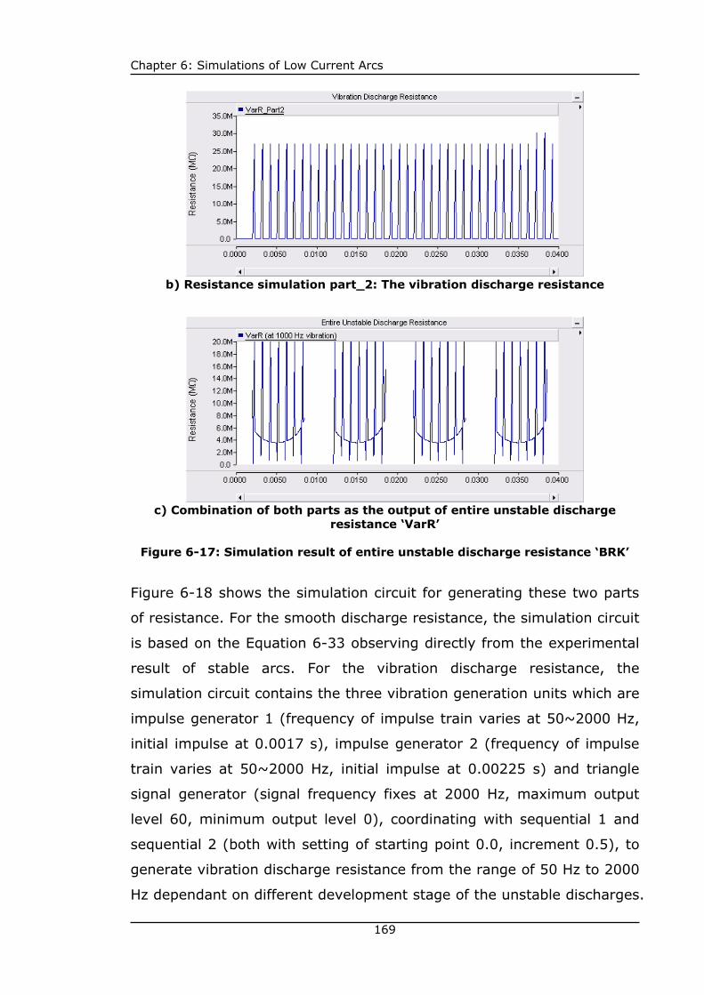
Chapter 6: Simulations of Low Current Arcs
169
b) Resistance simulation part_2: The vibration discharge resistance
c) Combination of both parts as the output of entire unstable discharge
resistance ‘VarR’
Figure 6-17: Simulation result of entire unstable discharge resistance ‘BRK’
Figure 6-18 shows the simulation circuit for generating these two parts
of resistance. For the smooth discharge resistance, the simulation circuit
is based on the Equation 6-33 observing directly from the experimental
result of stable arcs. For the vibration discharge resistance, the
simulation circuit contains the three vibration generation units which are
impulse generator 1 (frequency of impulse train varies at 50~2000 Hz,
initial impulse at 0.0017 s), impulse generator 2 (frequency of impulse
train varies at 50~2000 Hz, initial impulse at 0.00225 s) and triangle
signal generator (signal frequency fixes at 2000 Hz, maximum output
level 60, minimum output level 0), coordinating with sequential 1 and
sequential 2 (both with setting of starting point 0.0, increment 0.5), to
generate vibration discharge resistance from the range of 50 Hz to 2000
Hz dependant on different development stage of the unstable discharges.

Chapter 6: Simulations of Low Current Arcs
170
The combination circuit is used to combine the two parts of resistance
together in order to obtain the entire unstable discharge resistance
‘VarR’ shown in Figure 6-17 c).
Figure 6-18: Simulation circuit for entire unstable discharge resistance
( ) 3.0( )( ) 0.85sin 0.314
= =( )
aa
a
u tr ti t t
MΩ 6-33
6.3.3 PSCAD SIMULATION RESULTS FOR UNSTABLE DISCHARGES
Based on the simulation circuit and control circuit stated from part 6.3.1
and 6.3.2, the simulation results for unstable discharges and the
transforming process from unstable status to stable arc are shown in
Figure 6-19, together with the relative experimental results from the
Tests with Artificial Wind and Rain.

Chapter 6: Simulations of Low Current Arcs
171
Stage 1: a) Initial unstable discharges with vibration frequency at 2000 Hz
Stage 2: a) Unstable discharges with reduced vibration frequency to 1000 Hz
Stage 3: a) Stable arcs appear accompany with vibration frequency at 500 Hz
b) Experimental result at stage 3
a)
-20
-15
-10
-5
0
5
10
15
20
0 5 10 15 20 25 30 35 40
Time (ms)
Volta
ge (k
V)
-2
-1.5
-1
-0.5
0
0.5
1
1.5
2
Cur
rent
(mA)
VoltageCurrent
Vpeak=10 kV, Ipeak=0.8 mA, R=8 MΩWind speed=10 mph, Weak spray
b) Experimental result at stage 2
a)
-20
-15
-10
-5
0
5
10
15
20
0 5 10 15 20 25 30 35 40
Time (ms)
Volta
ge (k
V)
-2
-1.5
-1
-0.5
0
0.5
1
1.5
2
Cur
rent
(mA)
VoltageCurrent
Vpeak=10 kV, Ipeak=0.8 mA, R=8 MΩWind speed=10 mph, Weak spray
-20
-15
-10
-5
0
5
10
15
20
0 5 10 15 20 25 30 35 40
Time (ms)
Volta
ge (k
V)
-2
-1.5
-1
-0.5
0
0.5
1
1.5
2
Cur
rent
(mA)
VoltageCurrent
Vpeak=10 kV, Ipeak=0.8 mA, R=8 MΩWind speed=10 mph, Weak spray
b) Experimental result at stage 1
a)

Chapter 6: Simulations of Low Current Arcs
172
Stage 4: a) Stable arcs dominate with reduced vibration frequency to 200 Hz
Figure 6-19: Simulation result of unstable discharges
The correlation coefficients ‘r’ between the simulation and experiment
results of unstable discharges show r=0.69 for the voltage and r=0.76
for the current in stage 1; r=0.69 for the voltage and r=0.75 for the
current in stage 2; r=0.67 for the voltage and r=0.83 for the current in
stage 3; r=0.76 for the voltage and r=0.89 for the current in stage 4. In
the real situation, the vibrations in the experimental results are random
in each power cycles from stage 1 to 4, and difficult to be predicted in
the simulation conditions. However, the PSCAD simulation here can
reflect the main feature of unstable discharge phenomenon based on the
experimental test circuit.
6.3.4 ARC ENERGY AND ENERGY DENSITY FROM UNSTABLE DISCHARGES TO STABLE ARCS
Based on the PSCAD simulation of unstable discharges become stable
arcs, the energy trend during this process for respective four stages was
calculated and shown in Figure 6-20, together with the previous
experimental result from Figure 5-43 of the Tests with Artificial Wind
and Rain in section 5.4. Result shows the agreed increase trends of
energy for both experiment and simulation results, from unstable
discharges to stable status. The simulation stage 1 (2000 Hz vibration
discharges), stage 2 (reduced 1000 Hz vibration discharges) and part of
b) Experimental result at stage 4
a)
-20
-15
-10
-5
0
5
10
15
20
0 5 10 15 20 25 30 35 40
Time (ms)
Volta
ge (k
V)
-2
-1.5
-1
-0.5
0
0.5
1
1.5
2
Cur
rent
(mA)
VoltageCurrent
Vpeak=10 kV, Ipeak=0.8 mA, R=8 MΩWind speed=10 mph, Weak spray

Chapter 6: Simulations of Low Current Arcs
173
stage 3 (stable arc appears with 500 Hz vibration) could be classified as
unstable discharge period according to experiment results. The rest
simulation stage 4 (stable arc with lower than 500 Hz vibration) falls
into the experiment indicated stable arc period with energy higher than
0.01 Joule per cycle.
0
0.005
0.01
0.015
0.02
0 1 2 3 4 5 6 7 8 9 10Time after wind injection (s)
Arc
ene
rgy
per c
ycle
(Jou
le)
unstable discharge
stable arc
Vpeak=10 kV; Ipeak=0.8 mA; R=8 MΩ; Wind_speed=10 Mph; Weak spray
Experiment result
PSCAD simulationstage 1
stage 2
stage 3
stage 4
Figure 6-20: Arc energy trends from unstable discharges to stable arcs for
both PSCAD simulation and experiment results
Figure 6-21 shows the energy density trends of unstable discharges
becoming stable for the PSCAD simulation and experiment results. Both
results show the similar trends that during the discharge status
changing from unstable to stable, the energy density increases by an
order of 10 times from initial unstable discharges to final stable arcs,
which may give harmful effects on the insulation material surface due to
this transformation process.

Chapter 6: Simulations of Low Current Arcs
174
0
0.01
0.02
0.03
0.04
0.05
0.06
0.07
0.08
0.09
0.1
0 1 2 3 4 5 6 7 8 9 10Time after wind injection (s)
Ener
gy d
ensi
ty (J
oule
/cm
)
unstable discharge
stable arc
Vpeak=10 kV; Ipeak=0.8 mA; R=8 MΩ; Wind_speed=10 Mph; Weak spray
Experiment result
PSCAD simulation
stage 1
stage 2
stage 3
stage 4
Figure 6-21: Energy density trends from unstable discharges to stable arcs for
both PSCAD simulation and experiment results
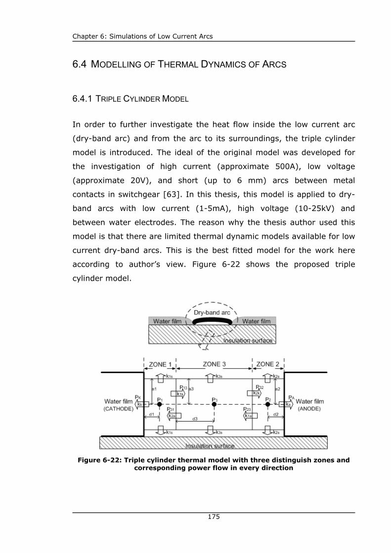
Chapter 6: Simulations of Low Current Arcs
175
6.4 MODELLING OF THERMAL DYNAMICS OF ARCS
6.4.1 TRIPLE CYLINDER MODEL
In order to further investigate the heat flow inside the low current arc
(dry-band arc) and from the arc to its surroundings, the triple cylinder
model is introduced. The ideal of the original model was developed for
the investigation of high current (approximate 500A), low voltage
(approximate 20V), and short (up to 6 mm) arcs between metal
contacts in switchgear [63]. In this thesis, this model is applied to dry-
band arcs with low current (1-5mA), high voltage (10-25kV) and
between water electrodes. The reason why the thesis author used this
model is that there are limited thermal dynamic models available for low
current dry-band arcs. This is the best fitted model for the work here
according to author’s view. Figure 6-22 shows the proposed triple
cylinder model.
Figure 6-22: Triple cylinder thermal model with three distinguish zones and
corresponding power flow in every direction

Chapter 6: Simulations of Low Current Arcs
176
When the dry-band arcing occurs, the water film has been divided into
two parts by the dry-band on the material surface. The edge of those
two water film can be considered as cathode and anode electrodes
respectively, while the dry-band area is assumed to be an air gap
between these two electrodes at atmosphere pressure. In this model,
three zones are identified as follows:
ZONE 1: CATHODE SPOT REGION (NEAR CATHODE ARC ZONE)
Zone 1 is defined as the ‘cathode spot region’ which is cylinder shaped
with radius a1 and length 2xd1. A concentrated source of heat P1 is
located in the geometrical centre of the cylinder. PK is the power
delivered to the cathode. P13 and P31 are the power transported to or
from zone 3. kk is the coefficient of heat penetration to the cathode. k1k
is the coefficient of the power flow from zone 1 to zone 3. k2a is the
coefficient of power flow from zone 3 to zone 1. k1s is coefficient of
power flow from zone 1 to the insulation surface.
ZONE 2: ANODE SPOT REGION (NEAR ANODE ARC ZONE)
Zone 2 is named as the ‘anode spot region’ which is cylinder shaped
with radius a2 and length 2xd2. A concentrated source of heat P2 is
located in the geometrical centre of the cylinder. Pa is the power
delivered to the anode. P23 and P32 are the power transported to or from
zone 2. ka is the coefficient of heat penetration to the anode. k1a is the
coefficient of power flow from zone 2 to zone 3. k2k is the coefficient of
power flow from zone 3 to zone 2. k2s is the coefficient of power flow
from zone 2 to the insulation surface.
ZONE 3: ARC COLUMN (CENTRAL ARC ZONE)
Zone 3 is named as the ‘arc column’ which is cylinder shaped with
radius a3 and length 2xd3. A concentrated source of heat P3 is located in
the geometrical centre of the cylinder. K3s is the coefficient of power
flow from zone 3 to the insulation surface.

Chapter 6: Simulations of Low Current Arcs
177
6.4.2 THERMAL FLOW CALCULATION
The modelling calculation is based on the arcing zones 1, 2 and 3
specified in the previous section. In each cylinder zone, a concentrated
source of heat (P1, P2 or P3) dissipates heat energy to both the cylinder
lateral surfaces and cylinder faces as demonstrated in Figure 6-23.
Figure 6-23: Energy flow calculation for one cylinder model (each arcing zone) [63]
According to Figure 6-23 b), the total power flowing through the cylinder
lateral surface is [63]
2 2
=+
b cdP P
a d 6-34
Where: Pb is the power flowing through the cylinder lateral surface, Pc is
the source power, a is the cylinder radius and d is half of the cylinder
length.
According to Figure 6-23 c), the power flowing through one of the
cylinder faces is [63]
2 2
1 (1 )2
= −+
p cdP P
a d 6-35
Where: Pp is the power flowing through the cylinder face.
a) Cylinder model with Pc
b) Power flowing through cylinder lateral surface
c) Power flowing through cylinder
face
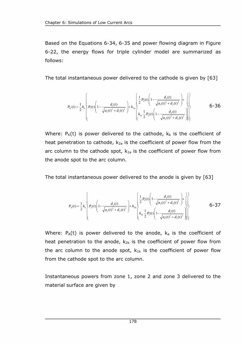
Chapter 6: Simulations of Low Current Arcs
178
Based on the Equations 6-34, 6-35 and power flowing diagram in Figure
6-22, the energy flows for triple cylinder model are summarized as
follows:
The total instantaneous power delivered to the cathode is given by [63]
3
3 2 23 31
1 22 21 1 2
1 2 2 22 2
( )1 ( ) 12 ( ) ( )( )1( ) ( ) 1
2 ( ) ( ) ( )1 ( ) 12 ( ) ( )
⎧ ⎫⎧ ⎫⎛ ⎞⎪ ⎪⎪ ⎪⎜ ⎟− +
⎜ ⎟⎪ ⎪⎪ ⎪⎛ ⎞ +⎪ ⎪ ⎪⎪⎝ ⎠⎜ ⎟= − +⎨ ⎨ ⎬⎬⎜ ⎟ ⎛ ⎞+⎪ ⎪ ⎪⎪⎝ ⎠ ⎜ ⎟−⎪ ⎪ ⎪⎪⎜ ⎟+⎪ ⎪ ⎪⎪⎝ ⎠⎩ ⎭⎩ ⎭
K k a
a
d tP ta t d td tP t k P t k
a t d t d tk P ta t d t
6-36
Where: PK(t) is power delivered to the cathode, kk is the coefficient of
heat penetration to cathode, k2a is the coefficient of power flow from the
arc column to the cathode spot, k1a is the coefficient of power flow from
the anode spot to the arc column.
The total instantaneous power delivered to the anode is given by [63]
3
3 2 23 32
2 22 22 2 1
1 1 2 21 1
( )1 ( ) 1-2 ( ) ( )( )1( ) ( ) 1-
2 ( ) ( ) ( )1 ( ) 1-2 ( ) ( )
⎧ ⎫⎧ ⎫⎛ ⎞⎪ ⎪⎪ ⎪⎜ ⎟ +
⎜ ⎟⎪ ⎪⎪ ⎪⎛ ⎞ +⎪ ⎪ ⎪⎪⎝ ⎠⎜ ⎟= +⎨ ⎨ ⎬⎬⎜ ⎟ ⎛ ⎞+⎪ ⎪ ⎪⎪⎝ ⎠ ⎜ ⎟⎪ ⎪ ⎪⎪⎜ ⎟+⎪ ⎪ ⎪⎪⎝ ⎠⎩ ⎭⎩ ⎭
A a k
k
d tP ta t d td tP t k P t k
a t d t d tk P ta t d t
6-37
Where: PA(t) is power delivered to the anode, ka is the coefficient of
heat penetration to the anode, k2k is the coefficient of power flow from
the arc column to the anode spot, k1k is the coefficient of power flow
from the cathode spot to the arc column.
Instantaneous powers from zone 1, zone 2 and zone 3 delivered to the
material surface are given by

Chapter 6: Simulations of Low Current Arcs
179
3
3 2 23 3 1
1 1 1 2 2 21 12
1 2 2 22 2
( )1 ( ) 12 ( ) ( ) ( )( ) ( )
( ) ( )( )1 ( ) 12 ( ) ( )
⎧ ⎫⎧ ⎫⎛ ⎞⎪ ⎪⎪ ⎪⎜ ⎟− +
⎜ ⎟⎪ ⎪⎪ ⎪ ⎛ ⎞+⎪ ⎪ ⎪⎪⎝ ⎠ ⎜ ⎟= +⎨ ⎨ ⎬⎬⎜ ⎟⎛ ⎞ +⎪ ⎪ ⎪⎪⎝ ⎠⎜ ⎟−⎪ ⎪ ⎪⎪⎜ ⎟+⎪ ⎪ ⎪⎪⎝ ⎠⎩ ⎭⎩ ⎭
S s a
a
d tP ta t d t d tP t k P t k
a t d td tk P ta t d t
6-38
3
3 2 23 3 2
2 2 2 2 2 22 21
1 1 2 21 1
( )1 ( ) 12 ( ) ( ) ( )( ) ( )
( ) ( )( )1 ( ) 12 ( ) ( )
⎧ ⎫⎧ ⎫⎛ ⎞⎪ ⎪⎪ ⎪⎜ ⎟− +
⎜ ⎟⎪ ⎪⎪ ⎪ ⎛ ⎞+⎪ ⎪ ⎪⎪⎝ ⎠ ⎜ ⎟= +⎨ ⎨ ⎬⎬⎜ ⎟⎛ ⎞ +⎪ ⎪ ⎪⎪⎝ ⎠⎜ ⎟−⎪ ⎪ ⎪⎪⎜ ⎟+⎪ ⎪ ⎪⎪⎝ ⎠⎩ ⎭⎩ ⎭
S s k
k
d tP ta t d t d tP t k P t k
a t d td tk P ta t d t
6-39
1
3 1 1 2 21 1 3
3 3 2 23 32
1 2 2 22 2
( )1( ) ( ) 12 ( ) ( ) ( )( )
( ) ( )( )1 ( ) 12 ( ) ( )
⎧ ⎫⎛ ⎞⎪ ⎪⎜ ⎟+ − +
⎜ ⎟⎪ ⎪⎛ ⎞+⎪ ⎝ ⎠ ⎪⎜ ⎟= ⎨ ⎬⎜ ⎟⎛ ⎞ +⎪ ⎪⎝ ⎠⎜ ⎟−⎪ ⎪⎜ ⎟+⎪ ⎪⎝ ⎠⎩ ⎭
k
S s
a
d tP t k P ta t d t d tP t k
a t d td tk P ta t d t
6-40
Where: P1S(t), P2S(t) and P3S(t) are the power delivered to material
surface from zone 1, zone 2 and zone 3 respectively. k1S, k2S and k3S are
coefficients of heat penetration to material surface from zone 1, zone 2
and zone 3 respectively.
6.4.3 THERMAL FLOW FOR DRY-BAND ARC COMPRESSION
When the dry-band arc is compressed, three stages will be involved as
described in Figure 6-24. The model used changes in different stages of
compression as follows:
STAGE 1:
In the first stage, the length of arc column (zone 3) is reducing, while
the lengths of zone1 and zone2 are assumed unchanged. The thermal
calculation is based on the Three Cylinder model at this stage.
STAGE 2:
The arc length continues reducing until equal to the zone 1 and zone 2
lengths, when the arc column (zone 3) disappears. The Three Cylinder
model without zone 3 will then be used for heat flow calculation.

Chapter 6: Simulations of Low Current Arcs
180
STAGE 3:
In the final stage, zone1 and zone 2 are compressed equally until the
arc length reduces to zero.
a) Dry-band arc compression stage 1
b) Dry-band arc compression stage 2
c) Dry-band arc compression stage 3
Figure 6-24: Thermal modelling of dry-band arc compression
6.4.4 MODELLING PARAMETERIZATION FOR THE TRIPLE CYLINDER MODEL
a1, a2, a3 – THE CYLINDER RADIUS FOR ZONE 1, ZONE 2 AND ZONE 3
An assumption is made that a1(t)=a2(t)=a3(t) at all times during the
dry-band arcing and arcing compression process. This assumption is
supported by the literature [63] and made for simplification purposes.
ai(t) is calculated from

Chapter 6: Simulations of Low Current Arcs
181
1 2 3( ) ( ) ( ) ( )= = = L aa t a t a t K i t mA 6-41
Where: ia(t) is the instantaneous arc current, KL is the constant
coefficient so that the cylinder radius changes in time with the
instantaneous arc current. Proportionality is assumed so that a higher
current corresponds to a thicker arcing zone. KL can be determined from
the maximum value of a1(t) and the maximum available current of
ia(t)max. From the measurement of the water layer thickness based on
the specified salt-fog precipitation rate in the Testing with Inclined
Samples, a1(t)max≈1 mm. ia(t)max=1.89 mA according to the previous
test result with 0° slope angle, and so KL=(1 mm)/(1.89 mA)
=0.0005278 m/mA.
d1, d2, d3 – THE CYLINDER LENGTH FOR ZONE 1, ZONE 2 AND ZONE 3
An assumption is made that d1(t)=d3(t) at all times during the dry-band
arc and arcing compression process. d2(t) is changed with physical arc
length following the arc compression process. The following assumptions
are made: d1(t)=d3(t)=a1(t)=a3(t) when d2(t)≠ 0 (representing stage 1
during the arcing compression in part 6.4.3); 2d1(t)=2d3(t)=La/2 when
d2(t)=0 (representing the stage 2 and 3 during the arcing compression
in part 6.4.3). These assumptions are from [63] and for simplification.
u1(t), u2(t), u3(t) – THE VOTALGE DISTRIBUTIONS IN ZONE 1, ZONE 2 AND
ZONE 3
Voltage drops in zone 1, zone 2 and zone 3 are assumed to be identical
[63]. Therefore, u1(t)=u2(t)=u3(t)=ua(t)/3, where ua(t) is the
instantaneous arc voltage. This assumption is from [63] and for
simplification.

Chapter 6: Simulations of Low Current Arcs
182
i1(t), i2(t), i3(t) – THE CURRENT THROUGH ZONE 1, ZONE 2 AND ZONE 3
Current flowing through zone 1, zone 2 and zone 3 are assumed to be
identical. Therefore, i1(t)=i2(t)=i3(t)=ia(t), where ia(t) is the
instantaneous arc current.
p1(t), p2(t), p3(t) – THE POWER IN ZONE 1, ZONE 2 AND ZONE 3
p1(t), p2(t) and p3(t) are instantaneous concentrated power located in
the geometry centre of zone 1, zone 2 and zone 3 respectively. The
following equations p1(t)=u1(t)xi1(t), p2(t)=u2(t)xi2(t), p3(t)=u3(t)xi3(t)
are used to calculate p1(t), p2(t) and p3(t) in the modelling calculation.
kk, k1a, k2a, ka, k1k, k2k, k1s, k2s, k3s – Coefficients from Equations
6-36 to 6-40 in Triple Cylinder Model
According to the thermal measurement, the average arcing temperature
is around 300 °C. The edge of water film is up to 100 °C, for the reason
that the water evaporation and deposition rate are in the dynamic
balance, maintaining the water temperature to be approximately 100 °C.
Therefore, the heat transfer coefficients are ambitiously calculated as
100 °C/300 °C≈30%, which makes the values of kk, ka, k1s, k2s, k3s to
be 0.3. The coefficients of heat transfer between different arc regions
are set to K1a=k2a=k1k=20%, k2k=50% according to literature [63].
Table 6-12 summarizes all the coefficients used in the Triple Cylinder
Model described from Equations 6-36 to 6-40.

Chapter 6: Simulations of Low Current Arcs
183
Table 6-12: Calculated coefficients for Triple Cylinder Model [63] based on Testing with Inclined Samples
Slope Angle (DEG) Arc Length (cm) Kk K1a K2a Ka K1k K2k K1s K2s K3s
0° 2.32 0.3 0.2 0.2 0.3 0.2 0.5 0.3 0.3 0.3
5° 2.28 0.3 0.2 0.2 0.3 0.2 0.5 0.3 0.3 0.3
10° 2.16 0.3 0.2 0.2 0.3 0.2 0.5 0.3 0.3 0.3
15° 1.94 0.3 0.2 0.2 0.3 0.2 0.5 0.3 0.3 0.3
20° 1.81 0.3 0.2 0.2 0.3 0.2 0.5 0.3 0.3 0.3
25° 1.72 0.3 0.2 0.2 0.3 0.2 0.5 0.3 0.3 0.3
30° 1.45 0.3 0.2 0.2 0.3 0.2 0.5 0.3 0.3 0.3
35° 1.11 0.3 0.2 0.2 0.3 0.2 0.5 0.3 0.3 0.3
40° 0.00 0.3 ----- ----- 0.3 ----- ----- 0.3 0.3 -----
6.4.5 CALCULATION RESULTS FROM TRIPLE CYLINDER MODEL
The power distribution inside the arcing region and radiation from the
arcing plasma to its surrounding were calculated in Matlab and the
designed program shown in [Appendix 1.2]. These calculations were
based on the Triple Cylinder Model proposed from Equations 6-36 to
6-40, the parameters estimation from part 6.4.4, and test results of
current ia(t) and voltage ua(t) curves from Testing with Inclined Samples
as modelling input. Figure 6-25 gives examples of calculation results of
arc power radiation to different directions including to the insulation
material surface.
0
0.5
1
1.5
2
2.5
3
0 5 10 15 20 25 30 35 40Time (ms)
Arc
Pow
er (W
att)
PK Electrode separation 2.32 cm
0
0.5
1
1.5
2
2.5
3
0 5 10 15 20 25 30 35 40Time (ms)
Arc
Pow
er (W
att)
PA Electrode separation 2.32 cm

Chapter 6: Simulations of Low Current Arcs
184
a) Instantaneous power radiations for 2.32 cm arc length
b) Instantaneous power radiations for 1.94 cm arc length
0
0.5
1
1.5
2
2.5
3
0 5 10 15 20 25 30 35 40Time (ms)
Arc
Pow
er (W
att)
PK Electrode separation 1.94 cm
0
0.5
1
1.5
2
2.5
3
0 5 10 15 20 25 30 35 40Time (ms)
Arc
Pow
er (W
att)
PA Electrode separation 1.94 cm
0
0.5
1
1.5
2
2.5
3
0 5 10 15 20 25 30 35 40Time (ms)
Arc
Pow
er (W
att)
P1S Electrode separation 1.94 cm
0
0.5
1
1.5
2
2.5
3
0 5 10 15 20 25 30 35 40Time (ms)
Arc
Pow
er (W
att)
P2S Electrode separation 1.94 cm
0
0.5
1
1.5
2
2.5
3
0 5 10 15 20 25 30 35 40Time (ms)
Arc
Pow
er (W
att)
P3S Electrode separation 1.94 cm
0
0.5
1
1.5
2
2.5
3
0 5 10 15 20 25 30 35 40Time (ms)
Arc
Pow
er (W
att)
P1S Electrode separation 2.32 cm
0
0.5
1
1.5
2
2.5
3
0 5 10 15 20 25 30 35 40Time (ms)
Arc
Pow
er (W
att)
P2S Electrode separation 2.32 cm
0
0.5
1
1.5
2
2.5
3
0 5 10 15 20 25 30 35 40Time (ms)
Arc
Pow
er (W
att)
P3S Electrode separation 2.32 cm

Chapter 6: Simulations of Low Current Arcs
185
c) Instantaneous power radiations for 1.72 cm arc length
0
0.5
1
1.5
2
2.5
3
0 5 10 15 20 25 30 35 40Time (ms)
Arc
Pow
er (W
att)
PK Electrode separation 1.11 cm
0
0.5
1
1.5
2
2.5
3
0 5 10 15 20 25 30 35 40Time (ms)
Arc
Pow
er (W
att)
PA Electrode separation 1.11 cm
0
0.5
1
1.5
2
2.5
3
0 5 10 15 20 25 30 35 40Time (ms)
Arc
Pow
er (W
att)
P1S Electrode separation 1.11 cm
0
0.5
1
1.5
2
2.5
3
0 5 10 15 20 25 30 35 40Time (ms)
Arc
Pow
er (W
att)
P2S Electrode separation 1.11 cm
0
0.5
1
1.5
2
2.5
3
0 5 10 15 20 25 30 35 40Time (ms)
Arc
Pow
er (W
att)
PK Electrode separation 1.72 cm
0
0.5
1
1.5
2
2.5
3
0 5 10 15 20 25 30 35 40Time (ms)
Arc
Pow
er (W
att)
PA Electrode separation 1.72 cm
0
0.5
1
1.5
2
2.5
3
0 5 10 15 20 25 30 35 40Time (ms)
Arc
Pow
er (W
att)
P1S Electrode separation 1.72 cm
0
0.5
1
1.5
2
2.5
3
0 5 10 15 20 25 30 35 40Time (ms)
Arc
Pow
er (W
att)
P2S Electrode separation 1.72 cm
0
0.5
1
1.5
2
2.5
3
0 5 10 15 20 25 30 35 40Time (ms)
Arc
Pow
er (W
att)
P3S Electrode separation 1.72 cm

Chapter 6: Simulations of Low Current Arcs
186
d) Instantaneous power radiations for 1.11 cm arc length
Figure 6-25: Result of calculated power radiation from zone 1, zone 2 and
zone 3 to cathode (PK), anode (PA), and insulation material surfaces (P1S, P2S, P3S)
Based on the calculation results of instantaneous power radiations; the
total energy dissipation in all directions from the arc can be calculated
by using Equation 6-42 in Matlab [program in Appendix 1.3], and the
results are shown in Table 6-13.
0
( )= ∫T
E P t tdt 6-42
Where: E is the accumulated energy for one power cycle of dry-band
arcing. T is 20 ms. P(t) is the instantaneous arc power radiation for each
direction calculated shown in Figure 6-25.
Table 6-13: Energy radiation from dry-band arcing to surroundings in a power cycle
Arc Length Energy to
Cathode
Energy to
Anode
Cathode to
Insulation
Surface
Anode to
Insulation
Surface
Column to
Insulation
Surface
La [cm] EK [Joule] EA [Joule] E1S [Joule] E2S [Joule] E3S [Joule]
2.32 0.001622 0.00167 0.00772 0.007789 0.011478
2.28 0.001944 0.002002 0.009254 0.009337 0.013758
2.16 0.002045 0.002106 0.009733 0.00982 0.014466
1.94 0.002429 0.002503 0.011561 0.011665 0.017175
1.81 0.002483 0.002559 0.011818 0.011925 0.017547
1.72 0.00269 0.002772 0.012802 0.012919 0.019005
1.45 0.002893 0.002984 0.013766 0.013893 0.020408
1.11 0.002964 0.003061 0.014091 0.014228 0.020821
0
0.5
1
1.5
2
2.5
3
0 5 10 15 20 25 30 35 40Time (ms)
Arc
Pow
er (W
att)
P3S Electrode separation 1.11 cm

Chapter 6: Simulations of Low Current Arcs
187
Figure 6-26 shows the examples of energy dissipation extracted from
Table 6-13. The energy calculation results show that following the dry-
band arc compression process, the energy dissipations in all directions
from the arc (EK, EA, E1S, E2S and E3S) are increased. E1S, E2S and E3S,
which are respective energy radiations from cathode, anode and arc
column to insulation material surfaces, give the largest contribution.
0
0.005
0.01
0.015
0.02
0.025
Ene
rgy
(Jou
le)
Arc Length 2.32 cmArc Length 2.28 cmArc Length 2.16 cmArc Length 1.94 cmArc Length 1.81 cmArc Length 1.72 cmArc Length 1.45 cmArc Length 1.11 cm
EK EA E1S E2S E3S *(EK=Energy to Cathode, EA=Energy to Anode, E1S=Cathode to Insulation Surface,
E2S=Anode to Insulation Surface, E3S=Column to Insulation Surface)
Figure 6-26: Modelling results of dry-band arcing energy for different radiation directions

Chapter 6: Simulations of Low Current Arcs
188
6.5 SUMMARY
The two simulation approaches, which are the respective Double
Sinusoidal Model and PSCAD simulation, have been proposed to
simulate low current dry-band arcing events. The Double Sinusoidal
Model was based on test results from Chapter 5 of the Thesis
Experimental Part, while the PSCAD simulation was based on the test
circuit arrangement for variable testing conditions. The outcome of
simulated current and voltage curves from both simulation approaches
show good correlation with experimental data, for the different
situations of stable arcs, arc compression and process of unstable
discharges becoming stable. The simulation work agrees with
experimental work showing that a dry-band arc will become more
detrimental if it is transformed from unstable discharges to stable arcs,
or physically compressed in length, for any reason.
The Triple Cylinder Model [63], which integrates the Double Sinusoidal
Model as the input data, is able to calculate the energy flow inside the
arc region and from arc to its environment. This thermal modelling work
indicates that when the arc is compressed in length due to external
movement of adjacent moisture for the reason either by gravity or wind,
the arc energy radiation is enhanced in all the directions from the arc
plasma to its surrounding. The worst case may happen when the arc
length is extremely short, which could increase the possibility of damage
to the substrate. The instantaneous arc power and accumulated arc
energy in the middle of arcing area facing the material surface are
highest. Therefore, the material may suffer more damage across that
region. The energy dissipation to both water electrodes (edge of two
water films) is lower than other directions. The compression of naturally
occurring dry-band arcs may therefore consequently accelerate the
material ageing process.

Chapter 8: Conclusion
189
7CHAPTER 7
DISCUSSION
7.1 LONG-TERM LOW CURRENT AGEING WITHOUT DISCHARGES
The research on a retired ADSS cable after 15 years’ service found
evidence of surface degradation under long-term low current ageing.
The visual observation verified no major ageing signs were contributed
from electrical discharges. However, the contact angle measurement
revealed the cable sheath had lost its hydrophobicity, and this surface
change was non-uniform and variable along the entire cable span.
Further electric field calculation successfully correlated with cable
surface degradation indicating that long term low leakage current could
possibly reduce the surface quality of outdoor insulation materials. This
is the first of such observation. The main reason for this form of
degradation may come from the long time Joule heating effect. The
surface sections which are subject to relatively higher leakage currents
may lose their hydrophobicity first, and in turn, allows moisture to be
more easily deposited. The moisture may further bring larger leakage
current passing through and again reduce the hydrophobicity on such
surface sections. Those two physical mechanisms may be further
affected and accelerated by each other, and eventually cause surface
degradation on outdoor insulations.
7.2 THE PROPERTIES OF LOW CURRENT ARCS
7.2.1 ARC STABILITY AND CURRENT
Research in [30] suggests that the arc voltage is only responsible for arc
ignition, and the arc energy (reflected by arc current) is the key factor

Chapter 8: Conclusion
190
to sustain an arc. In the Chapter 5 of Thesis Experimental Part, for the
cases of peak arcing currents higher than 1 mA, stable arcs are
observed with sustained arcing current and voltage profiles throughout
the whole arcing period, shown in Figure 5-5, Figure 5-17, Figure 5-32
and Figure 5-41. A special case appears in Figure 5-31 b) from the Tests
between Water Drops, with an unstable discharge observed under a 25
kV source voltage and between 1.0 cm electrode separation. In this case
the voltage is high enough to generate a discharge, but the electrode
separation is too large to sustain an arc. By reducing the water
electrode separation to 0.8 cm, a stable arc is observed.
The unstable discharges are observed for the discharge current below 1
mA in Figure 5-40 of the Tests with Artificial Wind and Rain. In this case
the current (energy) is insufficient to sustain an arc, so that the
discharge appears as ‘unstable’. These unstable discharges (with energy
less than 0.01 Joule per cycle) could be transformed into stable arcs
(with energy higher than 0.01 Joule per cycle) by external wind effect to
reduce the dry-band length, and therefore creating a shorter discharge
length. This transformation process has been successfully achieved in
experimental conditions even when the arcing current was less than 1
mA.
From the research in this thesis, it is clear that both factors of
insufficient arcing current (energy) and the long discharge length could
contribute to the instability of low current arcs. This unstable status
could be possibly transferred into a stable one by increasing the arc
current level or reducing the discharge route. The threshold current
(energy) between unstable and stable discharges is 1 mA (0.01 Joule
per cycle) according to the experimental work in this thesis.

Chapter 8: Conclusion
191
7.2.2 ARC LENGTH
Generally, arc length changes instantaneously with variable
instantaneous arc current available. However, in this research the
maximum available arc length for each power cycle were recorded and
used as ‘arc length’ for data acquisition and analysis. Therefore, each
half cycle of an arc corresponds to only one arc length and this
assumption is used throughout the whole thesis.
A balance can be achieved between arc heating to expand the dry-band
area and moisture deposition to reduce this area. In the experimental
situations, the arc heating effect can be adjusted by changing the values
of source voltage, and the available maximum arcing current which is
restricted by the current limiting resistor; while the moisture deposition
can be controlled by fog precipitation rate or spray flow rate. Therefore,
an ‘equilibrium arc length’ can be obtained after the balance is achieved,
with a fairly constant arc length observed in every consecutive power
cycles.
Arc length can be changed due to experimental conditions. For the of
Testing in a Fog Environment, the arc length extended following the
increase of source voltage, as a more powerful arc with higher voltage
and current level could produce more Joule heating to expand the dry-
band area, therefore increasing the arc length. In contrast, in the
Testing with Inclined Samples, the dry-band area was compressed in
length due to the gravity of upper water film on an inclined sample,
confining an arc length. The Tests between Water Drops manually
adjusted the water electrode separation to obtain the arcs with
‘expected’ lengths. In the Tests with Artificial Wind and Rain, by
changing moisture deposition such as increasing or decreasing rain
precipitation levels, or by modifying external forces such as enhancing
or weakening the wind injection, the arc length could also be changed.

Chapter 8: Conclusion
192
7.2.3 BREAKDOWN VOLTAGE
In the Thesis Experimental Part of Chapter 5, the relationships between
breakdown voltage and arc length were respectively shown in Figure
5-10 of Testing in a Fog Environment, Figure 5-19 of Testing with
Inclined Samples, Figure 5-33 of Tests between Water Drops and Figure
5-41 of Tests with Artificial Wind and Rain. All the results show the
similar trends that the breakdown voltage reduces when the arc length
(electrode separation) decreases: In the Testing in a Fog Environment,
the breakdown voltage increased following the rise of source voltage
leading to the expansion of dry-band length by more powerful arcs. In
the Testing with Inclined Samples, the breakdown voltage of an arc
dropped on more inclined samples as the dry-band arc was compressed
in length. In the Tests between Water Drops, the breakdown voltage
increased in case of the two droplets moving towards to each other,
shortening the water electrodes’ separation. In the Tests with Artificial
Wind and Rain, the breakdown voltage reduced corresponding to the arc
length reduction resulting from wind compression.
Breakdown voltage for a low current arc striking between water
electrodes also depends on the dynamic change of water droplet shape
under the electric fields. In the Tests between Water Drops, research
found that the breakdown voltage also changed with source voltage
levels for the same electrode separation, due to the ‘real’ arc length
change between mobile water electrodes. This arrangement of an arc
striking in the free air allowed more freedom for the water electrodes’
movement and distortion than the arcing activities on the solid
insulation surface. Therefore, no such phenomenon was observed in
other tests with the surface presence.

Chapter 8: Conclusion
193
7.2.4 ARCING PERIOD
The arcing period is the period from arc ignition to arc extinction. For
‘the free-growth arcs’ in the Testing in a Fog Environment, the arcing
period kept approximately constant for the different current levels from
1.5 mA to 4.0 mA (Figure 5-11), due to the breakdown voltage
increases with the source voltage to make the arc ignition time roughly
constant. For the ‘length-compressed arcs’ in Figure 5-17 of the Testing
with Inclined Samples, and in Figure 5-41 of the Tests with Artificial
Wind and Rain, the arcing period was prolonged corresponding to the
arc length reduction. This was due to the decrease in breakdown voltage
bringing forward the arc ignition time under the same source voltage.
But the arc extinction time did not change much according to the
experimental observations.
Research in this thesis indicates that the arcing period is a key factor for
the arc energy change as the arc striking for longer period may allow
more energy accumulation. This is also the main reason for the energy
increase during the arc compression process.
7.2.5 ARC RESISTANCE AND RESISTIVITY
The instantaneous arc resistance for stable arcs performed a ‘U’ shape in
the experimental works from Chapter 5. For the ‘free-growth arcs’ in the
Testing in a Fog Environment, the minimum value of instantaneous arc
resistance (Rmin) had similar values in the arcing levels of 1.5 mA to 4.0
mA in Figure 5-14, while the minimum instantaneous arc resistivity
(R’min) reduced significantly following the arcing level increases in Figure
5-15, due to the resultant expansion of dry-band arc length following
the rise of arc current and voltage. In contrast, for the ‘length-
compressed arc’ created in Testing with Inclined Samples, the trend of
Rmin reduced from an arc length of 2.32 cm to 1.11 cm during the arc

Chapter 8: Conclusion
194
compression process, while the R’min still kept fairly constant throughout.
This was due to the fixed R’min under the same source voltage and arc
current level, even in the arc compression situations. But the dry-band
area kept reducing during the process, leading to the drop of Rmin from 6
MΩ cm to 3.5 MΩ.
7.2.6 ARC ENERGY AND ENERGY DENSITY
The changes of arc energy and energy density were analyzed in the two
main situations: the unstable discharges becoming stable arcs and the
stable arcs being compressed in physical length. The first situation was
achieved by the Tests with Artificial Wind and Rain, with energy
calculation examples shown in Figure 5-42 and Figure 5-43,
demonstrating the arc energy could rise from less than 0.01 Joule per
cycle (unstable discharges) to higher than 0.01 Joule per cycle (stable
arcs) with up to 3 times increase during the process. The energy density
changes for the first situation were shown in Figure 5-46, with the order
of 10 times increase from unstable discharges to stable arcs. The second
arc compression situation was created respectively in both the Testing
with Inclined Samples and Tests with Artificial Wind and Rain. Both of
which showed the increase trend in arc energy following the arc length
compression for different arcing levels on inclined insulation surfaces in
Figure 5-28, and for arcs under the wind impact in Figure 5-44. For the
energy density analysis during the arc compression process, results
showed significant rise in energy density for different arcing levels on
inclined insulation surface up to 10 times from Figure 5-29, and up to 6
times’ increase due to the wind effected arc compression in Figure 5-47.
The arc energy and energy density trends in this thesis indicate that the
low current discharges could become more detrimental to insulation
material surfaces in terms of enhanced heat radiation under certain

Chapter 8: Conclusion
195
events, such as unstable discharges becoming stable and arc
compression in physical lengths.
7.3 MODELLING AND SIMULATION OF LOW CURRENT ARCS
7.3.1 MODELLING PARAMETER EXTRACTION FROM EXPERIMENTAL RESULTS
The data extraction was based on observing the experimental results in
terms of I-t and V-t curves stored in Excel files. Each power cycle
contained 800 points of sample data and the modelling parameters of
breakdown voltage, arc ignition time and voltage, arc extinction time
and voltage, arc current peak were obtained based on the digital values
of data group from Excel with Matlab programming to select the best fit
data. This method ensures better accuracy for the modelling of low
current discharges from the range of less than 1 mA to several mA.
7.3.2 MODELLING ASSUMPTIONS
The Double Sinusoidal Model for the modelling of dry-band arc
compression in section 6.2.1 made a few assumptions that the arcing
voltage was an inclined straight line during the arcing period and this
line was unchanged for the different arc length from 2.32 cm to 1.11 cm.
This assumption was for simplification and could reflect the main shape
of arcing voltage during the tests. The arc extinction time was also
assumed to be constant during the arc compression process, determined
by calculating the mean value of all cases from the Testing with Inclined
Samples. A similar assumption was made for angular frequency of
current sinusoidal wave to be a constant value throughout the arc
compression process, although the above parameters where slightly
changed with different arc length from the measurement results. Those
assumptions were all acceptable as the modelled I-t and V-t curves have

Chapter 8: Conclusion
196
shown high correlation with the experimental results summarized in
Table 6-10 and Table 6-11. However, the arc energy and energy
calculations still demonstrated some errors (less than 10%) compared
with experiment in Figure 6-13 and Figure 6-14.
The PSCAD simulations for low current stable arcs and arc compression
were conducted based on the experimental test circuits. Assumptions
were made that the current limiting resistor was unchanged for each of
simulation. Refering to the real experimental conditions, the current
limiting resistor did changed with temperature variation resulting from
leakage current during the testing period. The current limiting resistor
used for test may rise in temperature up to 20°C according to
measurement (within 12.5% of resistance change). This assumption for
the PSCAD simulation circuit was for simplification and proved to be
acceptable, as the evidence of high correlation with experimental results
were shown in Table 6-10 and Table 6-11. However, for the arc energy
and energy density calculations, errors (less than 10%) still existed
between PSCAD calculation results and experimental results, shown in
Figure 6-13 and Figure 6-14.
The PSCAD simulation for unstable discharges made the assumption
that the frequency of discharge voltage and current instability was
initially at 2000 Hz, and reduced towards stable arcs to a final 200 Hz.
This is an ambitious assumption that for the real testing cases in the
Tests with Artificial Wind and Rain, the unstable discharges varied by
every single power cycle and the exact shape of instability could be
hardly predicted. However, the PSCAD simulation based on this
assumption could reflect the main characteristics of unstable discharges
with evidence shown in Figure 6-17. But the correlation coefficients
between simulation and experiment results for unstable discharges (part
6.3.3) were not as accurate as for stable arcs.

Chapter 8: Conclusion
197
The Triple Cylinder Model for the modelling of thermal dynamics of arcs
made a few assumptions. First assumption was on three cylinder regions
identified as ‘Cathode spot region’, ‘Anode spot region’ and ‘Arc column’.
In the real situations, experimental work in Chapter 5 showed the arcing
region was changed by time with no constant appearance as either a
‘cylinder shape’ or ‘three distinguish regions’. This assumption was the
basic structure of this model and for reflecting the rough power flow
inside the arc and from arc to its surroundings. The second assumption
was made for the heat transfer coefficients inside the arc and from
arcing region to surroundings. The coefficients kk, ka, k1s, k2s, k3s were
determined by the evaluation of temperature difference between arc and
water films. This is an ambitious assumption and could reflect the basic
heat transfer coefficients from arcing region to insulation material
surfaces. The coefficients of heat transfer between different arc regions
which were respectively K1a, k2a, k1k, and k2k were taken from literature
[63]. This model was original designed for high current, low voltage arcs
and has limitation on the low current dry-band arc application. Due to
the difficulties in measuring the arc plasma temperature in every
directions, this model has not been verified through experimental
approaches.

Chapter 8: Conclusion
198
8CHAPTER 8
CONCLUSION In this thesis, the ageing phenomenon of outdoor insulation under low
leakage currents has been investigated. The research was focused on
the two main elements: the low current ageing without obvious
electrical discharges, and the low current arcs with extreme arcing
compression situations. Two kinds of methodologies have been used in
this research; these are classified as experimental study and simulation.
Experimental work conducted was: the contact angle measurement for
insulation surface examination, testing in a fog environment, testing on
the inclined samples, testing between water droplets and tests under
artificial wind and rain. The simulation work carried out was: electric
field calculations, Double Sinusoidal Model, Triple Cylinder Model, and
PSCAD simulation.
The Contact Angle Measurement and Electric Field Calculations provided
evidence that the long-term low leakage current could degrade the
ADSS cable sheath on a 132 kV transmission lines after 15 years of
service.
The Testing in a Fog Environment has experimentally established stable
dry-band arcs on insulation rod, identified the arcing development
stages, observed material surface property changes during the arc
formation, analyzed the arcing properties in terms of arc voltage and
breakdown voltage, arc current, arcing period, arc resistance and
resistivity. The salt-fog conditions have been identified as the most
severe conditions for low current dry-band arc growth.

Chapter 8: Conclusion
199
The Testing on the Inclined Samples has successfully created dry-band
arc compression events. Following the reduction of arc length, the
breakdown voltage reduced making the arcing period longer; the peak
of arc current increased following the drop of arc resistance. As a result,
both arc energy and energy density were dramatically increased which
might potentially bring severe heating effects to the insulation materials.
The Testing between Water Drops created conditions to study low
current arcing between water contacts with variable separation without
the influence of insulation surfaces. Unstable discharges were observed
in this test in situations which had enough voltage to ignite an arc but
insufficient current to sustain it. The trends of energy and energy
density showed significant increases following the reduction of arc
length between two droplets. This research proved that the ‘arc
compression’ retained its nature without the impact of insulation
surfaces, with both increase in arc power and energy resulting more
heating effect from arcing regions.
The Testing with Artificial Wind and Rain successfully provided other
environmental situation for low current arc (several mAs) compression,
and also the possible transformation from extreme low current unstable
discharges (lower than 1 mA) to stable arcs by the impact of wind. Both
the processes of arc compression and unstable discharges becoming
stable showed the arc energy and energy density could increase
significantly.
The simulation works developed a novel Double Sinusoidal Model to
simulate the voltage and current profiles of dry-band arc and its
compression process. The PSCAD simulation based on the experimental
circuits successfully simulated the test results from the fog
environmental tests, inclined sample tests, and artificial wind and rain
tests with high degrees of correlation. The Triple Cylinder Model was

Chapter 8: Conclusion
200
developed to calculate the heat radiation from arcs to their surroundings
especially to material surfaces. The simulation work successfully
replicates the experimental observation that during the arc compression
process, the arc energy and its density were dramatically increased, and
the heat radiation from arc to material surfaces were significantly
enhanced.
The final conclusion of this thesis is to confirm that the low current arc
compression phenomenon could have severe impact on surface
insulation. Therefore, the lifetime of the insulation materials could not
be only determined by the long-term ageing effect, but also rare events
such as low current arc compressions. Such extreme events may
dominate the insulation lifetime and cause unexpected failures to power
systems.

References
201
9CHAPTER 9
FUTURE WORK Future experimental work should focus on the real geometry of
insulators on overhead transmission lines, investigating low current
discharges on the more complex insulator surfaces and the possibility of
transformation from low energy arcs to certain extreme conditions such
as dry-band arc compression, or from unstable discharges to stable arcs,
both of which have been already discussed in this thesis. As discussed,
the materials may fail quicker when exposed to ‘normal’ low current
ageing conditions. Signs of degradation of transmission line elements
under such events may be reported in the future based on the theory
proposed in this thesis, and heightened awareness of the process.
Experimental work between water drops was found that the droplets
under AC electric field without an insulation surface may be highly
deformed, and this may affect the electrical behaviours of low current
arcs such as breakdown voltage and arc length. This phenomenon needs
to be further studied by applying high speed camera into experiment,
and the links between electric field strength, water distortion images
and arcing properties need to be further established.
Modelling work for low current discharges should be further developed.
Double sinusoidal model should expand its applications for simulating
arcs with higher current and voltage levels. The capability of such model
for wider applications needs to be assessed. The investigation also
needs to be conducted searching for the reason why currents during the
arcing period appear as sinusoidal waveforms, together with the
minimum arc resistance fairly constant with different current levels from
1 mA to 5 mA.

References
202
Thermal models should be further implemented by considering the real
shape of arcs. The distances from the arcing plasma to material surfaces
from cathode, anode and arc column are different, and that needs to be
taken into consideration. Due to the experimental limitations, difficulties
are existed to measure the thermal flow inside the arc and near
surrounding regions. Therefore, a new route needs to be found to
further verified the validly of thermal models and provide experimental
support for modelling parameters.
A new model should be built based on the physics of discharges, which
is able to help understanding the instability of discharges, and the
reason for transformation to more stable situations. Ideas of using static
arc resistance and investigating the relationship between this resistance
and arc length need to be further carried out for arc compression cases.

References
203
REFERENCES [1] J.S.T.Looms, Insulators for High Voltages. London: Peter Peregrinus Ltd, 1990. [2] J. F. Hall, "History and bibliography of polymeric insulators for outdoor
applications," IEEE Transactions on Power Delivery, vol. 8, pp. 376-385, 1993. [3] R. S. Gorur, E. A. Cherney, and J. T. Burnham, Outdoor Insulators. Phoenix,
Arizona, USA, 1999. [4] G. F. Moore, "Part 7: Optical Fibres in Power Transmission Systems," in Electric
Cables Handbook, 3rd Edition ed: Blackwell Science, 1997, pp. 685-752. [5] A. Haddad and D. Warne, Advanced in High Voltage Engineering. London: The
institution of Electrical Engineers, 2004. [6] C. N. Carter, J. Deas, N. R. Haigh, and S. M. Rowland, "Applicability of all-
dielectric self-supporting cable system to very high voltage overhead power lines," 46th Proc. International Wire and Cable Symposium, 1997, pp. 624-631.
[7] made-in-china.com. vol. 2010: http://image.made-in-china.com/2f0j00ZBEacGrJgfgm/25KV-Polymer-Suspension-Insulator.jpg, 26 Oct 2010.
[8] K. Kamo, T. Nakanishi, Y. Hayashi, and R. Matsuoka, "Reproducing tests of brittle fractures of polymer insulators," Proceedings of the 6th International Conference on Properties and Applications of Dielectric Materials, 2000, pp. 395-398 vol.1.
[9] S. Wu, Polymer interface and adhesion. New York: Technology & Engineering, 1982.
[10] N. E. Frost and M. Krenceski, "Hydrophobicity recovery in silicone insulators: a closer look at testing," IEEE International Symposium on Electrical Insulation, 2002, pp. 220-223.
[11] Y. Li, "Application of composite insulators in seriously contaminated areas," in Eleventh International Symposium on High Voltage Engineering(Conf. Publ. No. 467), 1999, pp. 180-183 vol.4.
[12] R. G. Houlgate and D. A. Swift, "Composite rod insulators for AC power lines: electrical performance of various designs at a coastal testing station," IEEE Transactions on Power Delivery, vol. 5, pp. 1944-1955, 1990.
[13] R. Hackam, "Outdoor HV composite polymeric insulators," IEEE Transactions on Dielectrics and Electrical Insulation, vol. 6, pp. 557-585, 1999.
[14] M. Kumosa, L. Kumosa, and D. Armentrout, "Failure analyses of nonceramic insulators Part 1: Brittle Fracture Characteristics," IEEE Electrical Insulation Magazine. vol. 21, May/June 2005, pp. 14-27.
[15] A. J. Davies, P. Radage, S. M. Rowland, and D. J. Walker, "The selection of materials for a long span, dielectric, aerial, self-supporting cable for optical communications," Plastics in Telecomms. vol. VI London, 1992, pp. 27/1-27/10.
[16] S. M. Rowland, K. Craddock, C. N. Carter, I. Houghton, and D. Delme-Jones, "The development of a metal-free, self-supporting, optical cable for use on long span, high voltage overhead power lines," in Proc 36th Int Wire and Cable Symposium, 1987, pp. 449-456.
[17] S. M. Rowland and F. Easthope, "Electrical ageing and testing of dielectric self-supporting cables for overhead power lines," IEE Proceedings-Science, Measurement and Technology, vol. 140, pp. 351-356, 1993.

References
204
[18] S. M. Rowland, "Sheathing materials for dielectric, aerial, self-supporting cables for application on high voltage power lines," 6th IEE Conference on Dielectric materials, Measurements and Applications, 1992, pp. 53-56.
[19] H. Ye, J. Zhang, Y. M. Ji, W. Y. Sun, K. Kondo, and T. Imakoma, "Contamination accumulation and withstand voltage characteristics of various types of insulators," Proceedings of the 7th International Conference on Properties and Applications of Dielectric Materials, 2003, pp. 1019-1023 vol.3.
[20] G. G. Karady, "Flashover mechanism of non-ceramic insulators," IEEE Transactions on Dielectrics and Electrical Insulation, vol. 6, pp. 718-723, 1999.
[21] E. A. Cherney and D. J. Stonkus, "Non-ceramic insulators for contaminated environments," IEEE Transactions on Power Apparatus and Systems, vol. PAS-100, pp. 131-142, 1981.
[22] S. E. Kim, E. A. Chemey, and R. Hackam, "Effect of dry band arcing on the surface of RTV silicone rubber coatings," in IEEE International Symposium on Electrical Insulation Baltimore, MD USA, 1992.
[23] A. J. Phillips, D. J. Childs, and H. M. Schneider, "Aging of nonceramic insulators due to corona from water drops," IEEE Transactions on Power Delivery, vol. 14, pp. 1081-1089, 1999.
[24] D. Windmar, "Water Drop Initiated Discharges in Air," Uppsala University. vol. PHD Thesis, 1994.
[25] A. J. Phillips, D. J. Childs, and H. M. Schneider, "Water drop corona effects on full-scale 500 kV non-ceramic insulators," IEEE Transactions on Power Delivery, vol. 14, pp. 258-265, 1999.
[26] K. Katada, Y. Takada, M. Takano, T. Nakanishi, Y. Hayashi, and R. Matsuoka, "Corona discharge characteristics of water droplets on hydrophobic polymer insulator surface," Proceedings of the 6th International Conference on Properties and Applications of Dielectric Materials, 2000, pp. 781-784 vol.2.
[27] I. J. S. Lopes, S. H. Jayaram, and E. A. Cherney, "A method for detecting the transition from corona from water droplets to dry-band arcing on silicone rubber insulators," IEEE Transactions on Dielectrics and Electrical Insulation, vol. 9, pp. 964-971, 2002.
[28] V. M. Moreno and R. S. Gorur, "Effect of long-term corona on non-ceramic outdoor insulator housing materials," IEEE Transactions on Dielectrics and Electrical Insulation, vol. 8, pp. 117-128, 2001.
[29] Y. Koshino, I. Umeda, and M. Ishiwari, "Deterioration of silicone rubber for polymer insulators by corona discharge and effect of fillers," Annual Report. Conference on Electrical Insulation and Dielectric Phenomena, 1998, pp. 72-79 vol. 1.
[30] Q. Huang, G. G. Karady, B. Shi, and M. Tuorninen, "Calculation of the electric field distribution on ADSS fiber optic Ccable," Conference on Electrical Insulation and Dielectric Phenomena, 2003, pp. 379-382.
[31] S. M. Rowland and I. V. Nichols, "Effects of dry-band arc current on ageing of self-supporting dielectric cables in high fields," IEE Proceedings -Science, Measurement and Technology, vol. 143, pp. 10-14, 1996.
[32] B. F. Hampton, "Flashover mechanism of polluted insulation," IEE Proceedings, pp. 985-990, 1964.
[33] X. Zhang, S. Rowland, and V. Terzija, "Increased energy in stable dry-band arcs due to length compression," IEEE Transactions on Dielectrics and Electrical Insulation, vol. 17, pp. 473-480.
[34] A. E. Guile, "The protection of high-voltage insulators from power-arc damage," Proceedings of the IEE - Part A: Power Engineering, vol. 108, pp. 317-323, 1961.
References
205
[35] P. Ranon, M. Kristiansen, F. Lehr, and L. Hatfield, "Insulator damage in high current discharges," IEEE Transactions on Magnetics, vol. 22, pp. 1695-1698, 1986.
[36] R. Matsuoka, K. Tanaka, H. Shinokubo, and J. T. Burnham, "Damage of nonceramic insulator end fittings by power arc currents," in IEEE 8th International Conference on Transmission & Distribution Construction, Operation & Live-Line Maintenance, 1998, pp. 278-284.
[37] C. L. Phan and M. Hara, "Leakage current and flashover performance of iced insulators," IEEE Transactions on Power Apparatus and Systems, vol. PAS-98, pp. 849-859, 1979.
[38] R. S. Gorur, A. D. L. O, H. El-Kishky, M. Chowdhary, H. Mukherjee, R. Sundaram, and J. T. Burnham, "Sudden flashover of nonceramic insulators in artificial contamination tests," IEEE Transactions on Dielectrics and Electrical Insulation, vol. 4, pp. 79-87, 1997.
[39] A. d. L. O and R. S. Gorur, "Flashover of contaminated nonceramic outdoor insulators in a wet atmosphere," Dielectrics and Electrical Insulation, IEEE Transactions on, vol. 5, pp. 814-823, 1998.
[40] K. Seog-Hyeon, E. A. Cherney, R. Hackam, and K. G. Rutherford, "Chemical changes at the surface of RTV silicone rubber coatings on insulators during dry-band arcing," IEEE Transactions on Dielectrics and Electrical Insulation, vol. 1, pp. 106-123, 1994.
[41] C. N. Carter, "Dry band electrical activity on optical cables strung on overhead power lines," in Proc. 37th International Wire and Cable Symposium, 1988, pp. 117-121.
[42] S. M. Rowland, "Prevention of dry-band arc damage on ADSS cables," IEEE Transactions on Dielectrics and Electrical Insulation, vol. 13, pp. 765-772, 2006.
[43] S. M. Rowland, "Engineering a solution to the aging of HV self-supporting cables by dry-band arcing," IEEE Electrical Insulation Magazine, vol. 22, pp. 33-43, 2006.
[44] F. Kaidanov, R.Munteanu, and G.Sheinfain, "Damages and destruction of fiber optic cables on 161 kV overhead transmission lines," IEEE Electrical Insulation Magazine, vol. 16, pp. 16-23, 2000.
[45] G. G. Karady, G. Besztercey, and M. W. Tuominen, "Corona caused deterioration of ADSS fiber-optic cables on high voltage lines," IEEE Transactions on Power Delivery, vol. 14, pp. 1438-1447, 1999.
[46] D. A. Brewer, L. A. Dissado, and M. J. Parry, "Limitations on the damage mechanism in dry band arcing on all dielectric self supporting cables," in Sixth International Conference on Dielectric Materials, Measurements and Applications, 1992, pp. 49-52.
[47] G. G. Karady, S. Baozhuang, H. Qi, D. Srinivasan, and M. W. Tuominen, "Experimental investigation of the aging process on ADSS optical fiber cables," in IEEE Power Engineering Society General Meeting, 2003, p. 228 Vol. 1.
[48] S. Baozhuang, G. G. Karady, H. Qi, and M. W. Tuominen, "Experimental studies of the characteristics of dry band arcing on ADSS fiber optic cables," IEEE Transactions on Power Delivery, vol. 19, pp. 1936-1940, 2004.
[49] X. Zhang, S. M. Rowland, and V. Terzija, "Increased energy in stable dry-band arcs due to length compression," IEEE Transactions on Dielectrics and Electrical Insulation, vol. 17, pp. 473-480.
[50] X. Zhang, "Analysis of High Voltage Optical Cable Performance," in The University of Manchester. vol. MSc Dissertation Manchester, 2007.
[51] ASTM D2303 Standard Test Methods for Liquid-Contaminant, Inclined-Plane Tracking and Erosion of Insulating Materials, Sep 10, 1997.

References
206
[52] L. H. Meyer, S. H. Jayaram, and E. A. Cherney, "Correlation of damage, dry band arcing energy, and temperature in inclined plane testing of silicone rubber for outdoor insulation," IEEE Transactions on Dielectrics and Electrical Insulation, vol. 11, pp. 424-432, 2004.
[53] S. M. Rowland and F. C. Lin, "Stability of alternating current discharges between water drops on insulation surfaces," J. Phys. D: Appl. Phys, vol. 39, pp. 3067-3076, 2006
[54] "IEC 1109 Standard: Artificial Pollution Tests on High Voltage Insulators to be Used in A.C. Systems."
[55] A. H. El-Hag, S. H. Jayaram, and E. A. Cherney, "Fundamental and low frequency harmonic components of leakage current as a diagnostic tool to study aging of RTV and HTV silicone rubber in salt-fog," IEEE Transactions on Dielectrics and Electrical Insulation, vol. 10, pp. 128-136, 2003.
[56] Y. Zhu, M. Otsubo, N. Anami, C. Honda, O. Takenouchi, Y. Hashimoto, and A. Ohono, "Change of polymeric material exposed to dry band arc discharge [polymer insulator applications]," in Annual Report Conference on Electrical Insulation and Dielectric Phenomena, 2004, pp. 655-658.
[57] A. H. El-Hag, "Detection of dry-band arcing using time series modeling [silicone rubber insulator arcing]," in Annual Report Conference on Electrical Insulation and Dielectric Phenomena, 2004, pp. 615-618.
[58] N. Anami, Y. Zhu, S. Hashimoto, M. Otsubo, C. Honda, O. Takenouchi, and Y. Hashimoto, "Evaluation of dry band arc on the polymeric insulator using differential technique and distortion factor of leakage current," in Annual Report. Conference on Electrical Insulation and Dielectric Phenomena, 2003, pp. 414-417.
[59] S. Baozhuang, H. Qi, G. G. Karady, and M. W. Tuominen, "Studies on the length of dry band arcs on ADSS fiber optic cables," in Annual Report. Conference on Electrical Insulation and Dielectric Phenomena, 2003, pp. 353-356.
[60] H. Qi, G. G. Karady, B. Shi, and M. Tuominen, "Numerical simulation of dry-band arcing on the surface of ADSS fiber optic cable," IEEE Transactions on Dielectrics and Electrical Insulation, vol. 12, pp. 496-503, 2005.
[61] V. Terzija and H. J. Koglin, "On the modeling of long arc in still air and arc resistance calculation," IEEE Transactions on Power Delivery, vol. 19, pp. 1012-1017, 2004.
[62] V. Terzija, G. Preston, M. Popov, and N. Terzija, "New static 'AirArc' EMTP model of long arc in free air," IEEE Transactions on Power Delivery, accepted for publication on 04/10/2010.
[63] P. Borkowski and E. Walczuk, "Thermal models of short arc between high current contacts," Proceedings of the Forty-Seventh IEEE Holm Conference on Electrical Contacts, 2001, pp. 259-264.
[64] S. M. Rowland, K. Kopsidas, and X. Zhang, "Aging of polyethylene ADSS sheath by low currents," IEEE Transactions on Power Delivery, vol. 25, pp. 947-952.
[65] S. M. Rowland, X. Zhang, and K. Kopsidas, "Ageing of an ADSS cable sheath on a 132kV overhead transmission line," in Annual Report Conference on Electrical Insulation and Dielectric Phenomena, 2008, pp. 192-195.

Appendix 1: Matlab Programs
207
APPENDIX 1: MATLAB PROGRAMS
APPENDIX 1.1
(Arc Energy calculation based on the measured I-t and V-t files)
clear; clc; column=0; % read V-t and I-t data from measurement results field as ‘1.log’, ‘2.log’, ‘3.log’…; each file contains 3200 rows, 2 columns, 4 power cycles of data. 1st column is voltage data group, 2nd column is current data group for dataNo=(1:40) %This example contains 40 recorded files of data data_name_part=int2str(dataNo); data_name=[data_name_part '.log']; IVdata=dlmread(data_name); % energy calculation for every half power cycles
Energyunit=0; for halfcycle=(1:8) % each files contains 8 half power cycles
for row=((halfcycle-1)*400+1:halfcycle*400) energyunit=energyunit+(IVdata(row,1)*IVdata(row,2)+IVdata(row+1,1)*IVdata(row+1,2))*0.025*0.001/2;
if row==halfcycle*400 column=column+1; energy_result(1,column)=energyunit; % write energy results energyunit=0; end
end end
end
APPENDIX 1.2
(Calculation of instantaneous power distribution based on the Triple
Cylinder Model)
clear datamax=xlsread('V I profile.xls') %load V I profile %parameter setting Kk=0.3 K1a=0.2 K2a=0.2 Ka=0.3 K1k=0.2 K2k=0.5 K1=0.2 K2=0.2

Appendix 1: Matlab Programs
208
K1s=0.3 K2s=0.3 K3s=0.3 KL=0.000528 Larcmax=0.0111 %arc length change by case %calculation start for i=1:1600 I(i)=abs(datamax(i,15)) %change by case V(i)=abs(datamax(i,16)) %change by case P1(i)=0.001*1/3*V(i)*I(i) P2(i)=0.001*1/3*V(i)*I(i) P3(i)=0.001*1/3*V(i)*I(i) a1(i)=KL*I(i) a2(i)=a1(i) a3(i)=a1(i) d1(i)=a1(i) d2(i)=a1(i) d3(i)=Larcmax-d1(i)-d2(i) end for t=1:1600 if (I(t)==0)|(V(t)==0) Pk(t)=0 Pa(t)=0 P1s(t)=0 P2s(t)=0 P3s(t)=0 else Pk(t)=1/2*Kk*(P1(t)*(1-d1(t)/sqrt(a1(t)^2+d1(t)^2))+K2a*(1/2*P3(t)*(1-d3(t)/sqrt(a3(t)^2+d3(t)^2))+K1a*1/2*P2(t)*(1-d2(t)/sqrt(a2(t)^2+d2(t)^2)))) Pa(t)=1/2*Ka*(P2(t)*(1-d2(t)/sqrt(a2(t)^2+d2(t)^2))+K2k*(1/2*P3(t)*(1-d3(t)/sqrt(a3(t)^2+d3(t)^2))+K1k*1/2*P1(t)*(1-d1(t)/sqrt(a1(t)^2+d1(t)^2)))) P1s(t)=K1s*(P1(t)+K2a*(1/2*P3(t)*(1-d3(t)/sqrt(a3(t)^2+d3(t)^2))+K1a*1/2*P2(t)*(1-d2(t)/sqrt(a2(t)^2+d2(t)^2))))*d1(t)/sqrt(a1(t)^2+d1(t)^2) P2s(t)=K2s*(P2(t)+K2k*(1/2*P3(t)*(1-d3(t)/sqrt(a3(t)^2+d3(t)^2))+K1k*1/2*P1(t)*(1-d1(t)/sqrt(a1(t)^2+d1(t)^2))))*d2(t)/sqrt(a2(t)^2+d2(t)^2) P3s(t)=K3s*(P3(t)+1/2*K1k*P1(t)*(1-d1(t)/sqrt(a1(t)^2+d1(t)^2))+1/2*K1a*P2(t)*(1-d2(t)/sqrt(a2(t)^2+d2(t)^2)))*d3(t)/sqrt(a3(t)^2+d3(t)^2) end end %data collection for n=1:1600 Result(n,1)=Pk(n) Result(n,2)=Pa(n) Result(n,3)=P1s(n) Result(n,4)=P2s(n) Result(n,5)=P3s(n) end

Appendix 1: Matlab Programs
209
APPENDIX 1.3 (Calculation of arc energy distribution based on the Triple Cylinder
Model)
clear % inital result Pk_result=0 Pa_result=0 P1s_result=0 P2s_result=0 P3s_result=0 datamax=xlsread('result_P.xls') % read Pk, Pa, P1s, P2s, P3s for 1600 % creat Pk, Pa, P1s, P2s, P3s data base for i=1:1600 Pk(i)=datamax(i,36) %change by case Pa(i)=datamax(i,37) %change by case P1s(i)=datamax(i,38) %change by case P2s(i)=datamax(i,39) %change by case P3s(i)=datamax(i,40) %change by case end % Calculate ENERGY for t=1:1599 Pk_result=Pk_result+1/2*(Pk(t)+Pk(t+1))*0.025 Pa_result=Pa_result+1/2*(Pa(t)+Pa(t+1))*0.025 P1s_result=P1s_result+1/2*(P1s(t)+P1s(t+1))*0.025 P2s_result=P2s_result+1/2*(P2s(t)+P2s(t+1))*0.025 P3s_result=P3s_result+1/2*(P3s(t)+P3s(t+1))*0.025 end % reformat for final result Final_result(1)=Pk_result Final_result(2)=Pa_result Final_result(3)=P1s_result Final_result(4)=P2s_result Final_result(5)=P3s_result

Appendix 2: List of Publications
210
APPENDIX 2: LIST OF PUBLICATIONS a) S. M. Rowland, X. Zhang, and K. Kopsidas, "The impact of system voltage on the
ageing of All-Dielectric Self-Supporting cables on overhead lines", 2008 IEEE International Symposium on Electrical Insulation, Vancouver, Canada, pp. 641-644, 2008.
b) S. M. Rowland, X. Zhang, and K. Kopsidas, "Ageing of an ADSS cable sheath on a 132kV overhead transmission line", Conference on Electrical Insulation and Dielectric Phenomena, CEIDP Annual Report, Quebec, Canada, pp. 192-195, 2008.
c) S. M. Rowland, K. Kopsidas, and X. Zhang, "Aging of polyethylene ADSS sheath by low currents," IEEE Transactions on Power Delivery, vol. 25, pp. 947-952, 2010.
d) X. Zhang, S. M. Rowland, and V. Terzija, "Increased energy in stable dry-band arcs due to length compression," IEEE Transactions on Dielectrics and Electrical Insulation, vol. 17, pp. 473-480, 2010.
e) X. Zhang and S. M. Rowland, “Dry-band arc compression and resultant arc energy changes,” 11th INSUCON International Electrical Insulation Conference, Birmingham, United Kingdom, pp. 308-313, 2009.
f) X. Zhang, S. M. Rowland and V. Terzija, “Modelling of dry-band arc compression”, 16th International Symposium on High Voltage Engineering, Cape Town, South Africa, pp. 284, 2009.
g) X. Zhang and S. M. Rowland, “Behaviour of low current discharges between water drops,” IEEE Conference on Electrical Insulation and Dielectric Phenomena, Virginia Beach, USA, pp. 437-440, 2009.
h) X. Zhang and S. M. Rowland, "Modelling of dry-band discharge events on insulation surfaces," 2010 IEEE International Symposium on Electrical Insulation (ISEI), San Diego, California, USA, pp. 1-5, 2010.
Related Documents


