Chapter 1 Implementation of a 2k factorial design in the ...

1

Chapter 1 Implementation of a 2k factorial design in the Flockado process applied to

automotive components

Capítulo 1 Implementación de un diseño factorial de 2k en el proceso de Flockado

aplicado a componentes automotrices

GALLARDO-GARCÍA, David, MÉNDEZ-MENDOZA, José Nemorio, VARELA-LOYOLA, José

Antonio and TOLAMATL-MICHCOL, Jacobo

Universidad Politécnica de Tlaxcala, Av. Universidad Politécnica #1 San Pedro Xalcaltzinco,

Tepeyanco, Tlaxcala, CP. 90180, México.

ID 1-Autor: David Gallardo-García / ORC ID: 0000-0001-5053-9109, Researcher ID Thomson: Q-

6227-2018, CVU CONACYT ID: 335582

ID 2-CoAutor: José Nemorio Méndez-Mendoza / ORC ID: 0000-0002-1991-9987, Researcher ID

Thomson: Q-6771-2018, arXiv ID: J_N_Mendez

ID 3-CoAutor: José Antonio Varela-Loyola / ORC ID: 0000-0002-4154-3170, Researcher ID

Thomson: Q-6654-2018, CVU CONACYT ID: 47128

ID 4-CoAutor: Jacobo Tolamatl-Michcol / ORC ID: 0000-0002-1435-7348, Researcher ID Thomson:

Q-4849-2018, CVU CONACYT ID: 334973

D. Gallardo, J. Méndez, J. Varela y J. Tolamatl

J. Tolamatl, D. Gallardo, J. Varela y J. Méndez. (Dir.) Strategies and successful practices of innovation in the automotive

industry, Science of technology and innovation. Handbooks-©ECORFAN-Mexico, Tlaxcala, 2018

2

Abstract

The quality of a product in the Automotive Industry demands that its suppliers comply with the

requirements in each of its mobile, rigid or joining components between the elements that make up the

function and operation of an automotive device; so in this study the adhesion operation of a mixture of

additives, catalysts and solvents for adhesion of microfibers (flock) of automotive parts is analyzed,

applying an Experiment Design (DoE) that allows an adhesion response and the final product present an

aesthetic and functional sensation to the geometry of the piece. The methodological process consists of

the application of the DoE that Montgomery (2005) proposes, the use of basic quality tools including the

analysis of the effect of failure in the operational process of adherence of the materials and the support

of the software Minitab 17 Statistical. The results obtained when implementing the DoE was a mixture

of 1100 ml for the adhesive, 900 ml for the catalyst and 1000 ml for the solvent to obtain a flock adhesion

of microfibers of a height of 0.9 mm in a time interval of 50 to 60 seconds.

Design of experiments, Flocking parts, Full factorial design

1. Introduction

In the Automotive Industry the manufacture of a product requires compliance with the Quality in each

of its components of an automotive device; so in this chapter; the problem that is the lack of adherence

of micro-fibers in the flock process, which requires optimizing the mixture of adhesion products on the

surface of the geometry of the piece. Flocking is the process of depositing microfibers on a surface. It

can also refer to the texture produced by the process, or to any material used mainly for surface adhesion

of the process. The flocking of an article can be done in order to increase its value in terms of tactile

sensation, aesthetics, color and appearance. It can also be performed for functional reasons such as

insulation, sliding friction, grip and low reflectivity. In the automotive industry flocking is used for

decorative purposes and can be applied to a number of different materials. The flock is the process of

adhering adhesives synthetic fibers with the appearance of fluff or microfibers in the geometry of interest

of the automotive component, once the impression of the flock to the touch feels velvety and with a

certain height. The length of the fibers can vary in thickness, which determines the appearance of the

flocked product.

A recurring problem detected in the flocking process is the detachment of microfibres allowing to

solve this lack of adherence by applying a factorial design in order to respond to this problem and to

define the reaction thickness (u) versus adhesive (ml), catalyst (ml) and Solvent (ml) for different levels

of the factor, identifying the optimal mixture of the adhesive, a problem that was decided to be addressed

by means of a 2K factorial design. The determination of the noise variables in the manufacturing process,

and the expected quality of the product were carried out, for this purpose statistical tools of quality,

analysis of the mode and effect of failure and a design of experiments were applied, later with the use of

the statistical package minitab version 17, the respective analyzes were performed determining the

response of the noise variables. Considering that a 2K factorial design is a methodological process that

can be defined as a test or series of tests in which deliberate changes are made in the input variables of a

process or system to observe and identify the reasons for the changes that could be observed in the output

response (Montgomery, 2005), derived from this conceptualization the response to an experiment of this

nature is the improvement to the process by detecting and minimizing the effects of the variance in the

factorial experiment. And as Correa and Medina (2011) says, the first step is to estimate the effect of the

factors, examine their signs and magnitudes; in this way the experimenter obtains preliminary

information about the factors and interactions that may be important and in which directions they should

adjust to improve the response.

1.1 Theoretical revision

The design of experiments according to Montgomery (2005), can be defined as a set of methods that are

used to manipulate a process in order to obtain information on how to improve it, in this way it is possible

to observe and identify the factors of changes in the response of departure. With this technique you can

get, for example, improve the performance of a process and reduce its variability or production costs. Its

application in the industry includes fields such as Chemistry, Mechanics, Materials, Industrial

Engineering or Electronics used in experimental sciences.

3

1.1.1 Historical review of the design of experiments

The design of experiments was applied for the first time by the statistician and biologist R. A. Fisher in

England in the 1920s in the field of agriculture; his experiences led him to publish in 1935 his book

Design of Experiments (DoE). Since then, several researchers have contributed to the development and

application of the technique in different fields. According to Montgomery, it is considered that there have

been four stages in the development of experimental design. The first stage initiated in the twenties by

Fisher is characterized by the systematic introduction of scientific thought and the application of

complete and fractional factorial design and analysis of variance in scientific experimental investigations.

The second stage - initiated by Box and Wilson 1951 - is characterized by the development of the

response surface (RSM). In their article Cervantes and Engstrom (2004) noted that industrial experiments

differed from those of agriculture in two aspects:

− Immediateness, because the answer can be observed quite quickly, without having to wait as long

as in agriculture.

− Sequentiality: the experimenter can perform a few experiments and plan the following depending

on the results.

In this last stage, designs like:

− Central composite designs (CCD).

− Central composite designs centered on the faces by three factors (CFD).

− Box-Behnken designs, response surface methodology (RSM) allows to optimize the experimental

process and other design techniques were extended to the chemical industry and industrial

processes, especially in the areas of research and development (R & D).

The third stage begins at the end of the seventies with the growing interest of the industries in the

improvement of their processes. The works of Taguchi on robust design of parameters (RPD) served to

spread the interest and the use of the Design of Experiments (DoE) other areas like automotive, aerospace

industry, electronics or semiconductor industry. According to Kackar (1989), although the analyzes

proposed by Taguchi were strongly criticized for being inefficient and in some cases ineffective, they

served to develop the concept of robustness and extend the use of the design of experiments to other

areas, which has started at the beginning of the fourth stage of experimental design in the nineties; in it,

optimal designs emerge and numerous software tools have been developed for the analysis of the DoE.

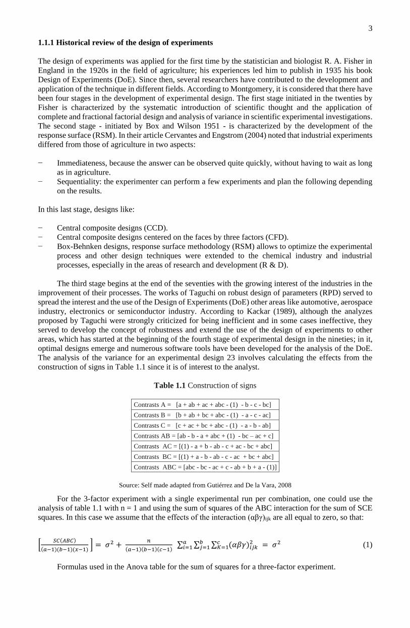
The analysis of the variance for an experimental design 23 involves calculating the effects from the

construction of signs in Table 1.1 since it is of interest to the analyst.

Table 1.1 Construction of signs

Contrasts A = [a + ab + ac + abc - (1) - b - c - bc]

Contrasts B = [b + ab + bc + abc - (1) - a - c - ac]

Contrasts C = [c + ac + bc + abc - (1) - a - b - ab]

Contrasts AB = [ab - b - a + abc + (1) - bc – ac + c]

Contrasts AC = [(1) - a + b - ab - c + ac - bc + abc]

Contrasts BC = [(1) + a - b - ab - c - ac + bc + abc]

Contrasts ABC = [abc - bc - ac + c - ab + b + a - (1)]

Source: Self made adapted from Gutiérrez and De la Vara, 2008

For the 3-factor experiment with a single experimental run per combination, one could use the

analysis of table 1.1 with n = 1 and using the sum of squares of the ABC interaction for the sum of SCE

squares. In this case we assume that the effects of the interaction (αβγ)ijk are all equal to zero, so that:

[𝑆𝐶(𝐴𝐵𝐶)

(𝑎−1)(𝑏−1)(𝑥−1) ] = 𝜎2 +

𝑛

(𝑎−1)(𝑏−1)(𝑐−1) ∑ ∑ ∑ (𝛼𝛽𝛾)𝑖𝑗𝑘

2𝑐𝐾=1 = 𝜎2𝑏

𝑗=1𝑎𝑖=1 (1)

Formulas used in the Anova table for the sum of squares for a three-factor experiment.

4

𝑆𝐶(𝐵𝐶) = 𝑎𝑛 ∑ ∑( �̅�.𝑗𝑘 . − �̅�.𝑗..

𝑘𝑗

– �̅�..𝑘 + �̅�…. )2 (2)

𝑆𝐶(𝐴𝐶) = 𝑏𝑛 ∑ ∑( �̅�.𝑖𝑘. − �̅�..𝑖…

𝑘𝑖

− �̅�..𝑘 + �̅�…. )2 (3)

𝑆𝐶(𝐴𝐵) = 𝑐𝑛 ∑ ∑( �̅�.𝑖𝑗. − �̅�..𝑖…

𝑗𝑖

− �̅�..𝑗 + �̅�…. )2 (4)

𝑆𝐶𝐴 = 𝑏𝑐𝑛 ∑( �̅�𝑖…

𝑎

𝑖=1

− �̅�…. )2

(5)

𝑆𝐶𝐵 = 𝑎𝑐𝑛 ∑( �̅�.𝑗..

𝑏

𝑗=1

− �̅�…. )2

(6)

𝑆𝐶𝐶 = 𝑎𝑏𝑛 ∑( 𝑦̅̅̅̅..𝑘.

𝑐

𝑘=1

− �̅�…. )2

(7)

𝑆𝐶(𝐴𝐵𝐶) = 𝑛 ∑ ∑ ∑(�̅�𝑖𝑗𝑘.

𝑘𝑗𝑖

− �̅�.𝑖𝑗.. − �̅�.𝑖𝑘.. − �̅�.𝑗𝑘. − �̅�.𝑖.. − �̅�.𝑗.. �̅�..𝑘. − �̅�…. )2 (8)

𝑆𝑇𝐶 = ∑ ∑ ∑ ∑(

𝑙

�̅�𝑖𝑗𝑘𝑙

𝑘𝑗𝑖

− �̅�…. )2 (9)

𝑆𝐶𝐸 = 𝑛 ∑ ∑ ∑(�̅�𝑖𝑗𝑘𝑙

𝑘𝑗𝑖

− �̅�𝑖𝑗𝑘. )2 (10)

The averages in the formulas are defined as follows:

�̅̅�... = Average of all abcn observations:

�̅�i... = Average of observations for the i-th level of factor A

�̅�.j.. = Average of observations for the j-th level of factor B,

�̅�..k. = Average observations for the kth level of factor C,

�̅� ij.. = Average of the observations for the i-th level of A and the j-th level of B,

�̅� i.k. = Average of the observations for the i-th level of A and the kth level of C,

�̅�.jk. = Average of the observations for the j-th level of B and the kth level of C.

�̅� ijk. = Average of the observations for the (ijk)-th treatment combination.

Table 1.2 ANOVA for the 3-factor experiment

Source of

Variation

Sum of

squares

Degrees of

freedom

Media square F

Calculated

Value p

Main effect:

A SCA a - 1 𝑆12

𝑓 =𝑠1

2

𝑠2

𝑝(𝑓 > 𝑓𝑜

B SAP b - 1 𝑆22

𝑓 =𝑠1

2

𝑠2


C SCC c - 1 𝑆32

𝑓 =𝑠1

2

𝑠2


Interaction of 2 factors:

AB SC(AB) ( a - 1 )( b - 1 ) 𝑆42

𝑓 =𝑠1

2

𝑠2


AC SC(AC) ( a - 1 )( c - 1 ) 𝑆52

𝑓 =𝑠1

2

𝑠2


AB SC(AB) ( a - 1 )( b - 1 ) 𝑆42

𝑓 =𝑠1

2

𝑠2


Interaction of 3 factors:

ABC SC(ABC) ( a - 1 )( b - 1 ) 𝑆72

𝑓 =𝑠1

2

𝑠2

Error SCE abc( n -1 )

Total STC abcn -1

Source: Adapted from Walpole, Ronald 2012

5

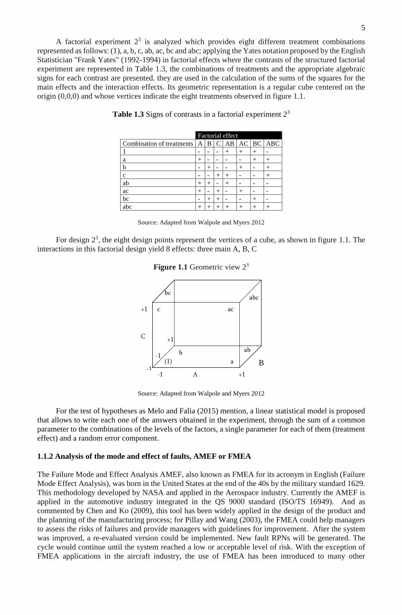
A factorial experiment 23 is analyzed which provides eight different treatment combinations

represented as follows: (1), a, b, c, ab, ac, bc and abc; applying the Yates notation proposed by the English

Statistician "Frank Yates" (1992-1994) in factorial effects where the contrasts of the structured factorial

experiment are represented in Table 1.3, the combinations of treatments and the appropriate algebraic

signs for each contrast are presented. they are used in the calculation of the sums of the squares for the

main effects and the interaction effects. Its geometric representation is a regular cube centered on the

origin (0,0,0) and whose vertices indicate the eight treatments observed in figure 1.1.

Table 1.3 Signs of contrasts in a factorial experiment 23

Source: Adapted from Walpole and Myers 2012

For design 23, the eight design points represent the vertices of a cube, as shown in figure 1.1. The

interactions in this factorial design yield 8 effects: three main A, B, C

Figure 1.1 Geometric view 23

Source: Adapted from Walpole and Myers 2012

For the test of hypotheses as Melo and Falia (2015) mention, a linear statistical model is proposed

that allows to write each one of the answers obtained in the experiment, through the sum of a common

parameter to the combinations of the levels of the factors, a single parameter for each of them (treatment

effect) and a random error component.

1.1.2 Analysis of the mode and effect of faults, AMEF or FMEA

The Failure Mode and Effect Analysis AMEF, also known as FMEA for its acronym in English (Failure

Mode Effect Analysis), was born in the United States at the end of the 40s by the military standard 1629.

This methodology developed by NASA and applied in the Aerospace industry. Currently the AMEF is

applied in the automotive industry integrated in the QS 9000 standard (ISO/TS 16949). And as

commented by Chen and Ko (2009), this tool has been widely applied in the design of the product and

the planning of the manufacturing process; for Pillay and Wang (2003), the FMEA could help managers

to assess the risks of failures and provide managers with guidelines for improvement. After the system

was improved, a re-evaluated version could be implemented. New fault RPNs will be generated. The

cycle would continue until the system reached a low or acceptable level of risk. With the exception of

FMEA applications in the aircraft industry, the use of FMEA has been introduced to many other

Factorial effect

Combination of treatments A B C AB AC BC ABC

1 - - - + + + -

a + - - - - + +

b - + - - + - +

c - - + + - - +

ab + + - + - - -

ac + - + - + - -

bc - + + - - + -

abc + + + + + + +

-1

abc

(1)

c

-1

bc

a

b ab

+1

-1

C

A

+1

+1

ac

B

6

industries. The purpose of the AMEF is to evaluate the reliability and control of the system, insofar as it

determines the potential effects of the failures, ranges of severity, occurrence and detection of the same.

This section considers that the Failure Mode and Effect Analysis tool is carried out in order to

identify in the output process the failure and the effect of experiencing those factors that impact the

specifications of the product in order to provide in the process productive an immediate and anticipated

response to the detected fault.

1.2 Materials and methods

A design of experiments involves much more than deciding what are the conditions in which each of the

experiments necessary to achieve the objective will be carried out; In addition, several stages must be

considered before and after the execution of such experiments. Throughout history several authors have

classified in different ways the necessary stages to apply the DoE (Drain, 1997). For the present chapter

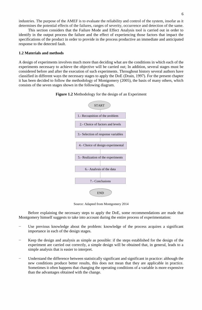
it has been decided to follow the methodology of Montgomery (2005), the basis of many others, which

consists of the seven stages shown in the following diagram.

Figure 1.2 Methodology for the design of an Experiment

Source: Adapted from Montgomery 2014

Before explaining the necessary steps to apply the DoE, some recommendations are made that

Montgomery himself suggests to take into account during the entire process of experimentation:

− Use previous knowledge about the problem: knowledge of the process acquires a significant

importance in each of the design stages.

− Keep the design and analysis as simple as possible: if the steps established for the design of the

experiment are carried out correctly, a simple design will be obtained that, in general, leads to a

simple analysis that is easier to interpret.

− Understand the difference between statistically significant and significant in practice: although the

new conditions produce better results, this does not mean that they are applicable in practice.

Sometimes it often happens that changing the operating conditions of a variable is more expensive

than the advantages obtained with the change.

1.- Recognition of the problem

END

2.- Choice of factors and levels

4.- Choice of design experimental

3.- Selection of response variables

5.- Realization of the experiments

7.- Conclusions

6.- Analysis of the data

END

START

7

− Remember that the experiments are iterative: generally, at the beginning of all experimentation you

do not have enough information to perform a completely correct analysis. Therefore it is

recommended not to invest more than 25-40% of the budget in the first experiments.

To better understand each of the stages of the methodology, these will be described in detail along

with some tips that can help carry them out (Montgomery, 2014).

1.2.1 Recognition of the problem

The first step to do a DoE is to recognize the problem. An undesirable situation in which something is

not working is understood as a problem. For Pande and Neuman (2000), the formulation of the problem

must be a concise and focused description of what is wrong; Whenever possible, it will be convenient to

quantify the problem in terms of cost, as this will make it possible to quantify the improvement achieved

at the end of the process. According to the problem raised, an analysis of the rejected lot was carried out

by the company, which consisted in carrying out a visual inspection. In accordance with the inspected

areas of the pieces, the areas where they presented the detachment are summarized with the help of a

Pareto diagram the areas where they had the flock release.

The total number of defective parts was 288 for the three shifts, which is equivalent to 57.6% in a

production of 500 pieces in a shift, this was alarming for the company, so a revision of a batch of 4

equivalent containers was carried out to 72 pieces so that they were re-processed of which the results are

shown in graphic 1.1:

Graphic 1.1 Flock detachment

Source: Self made with company data

As shown in graphic 1.1, the area with the greatest detachment was inside the piece, which should

be analyzed to determine how much the adhesive affects this defect. Once the situation has been analyzed,

the characteristics of the piece that are integrated in the work instruction are reviewed, with the objective

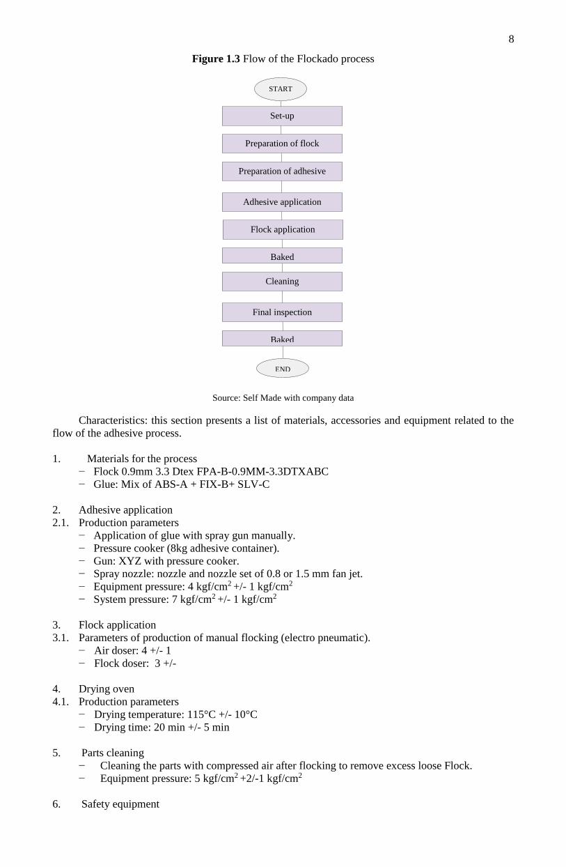
of analyzing the problem more easily. Next, figure 1.3 of the general flow of the process is presented,

showing the operations necessary to carry out the adhesive operation.

8

Figure 1.3 Flow of the Flockado process

Source: Self Made with company data

Characteristics: this section presents a list of materials, accessories and equipment related to the

flow of the adhesive process.

1. Materials for the process

− Flock 0.9mm 3.3 Dtex FPA-B-0.9MM-3.3DTXABC

− Glue: Mix of ABS-A + FIX-B+ SLV-C

2. Adhesive application

2.1. Production parameters

− Application of glue with spray gun manually.

− Pressure cooker (8kg adhesive container).

− Gun: XYZ with pressure cooker.

− Spray nozzle: nozzle and nozzle set of 0.8 or 1.5 mm fan jet.

− Equipment pressure: 4 kgf/cm2 +/- 1 kgf/cm2

− System pressure: 7 kgf/cm2 +/- 1 kgf/cm2

3. Flock application

3.1. Parameters of production of manual flocking (electro pneumatic).

− Air doser: 4 +/- 1

− Flock doser: 3 +/-

4. Drying oven

4.1. Production parameters

− Drying temperature: 115°C +/- 10°C

− Drying time: 20 min +/- 5 min

5. Parts cleaning

− Cleaning the parts with compressed air after flocking to remove excess loose Flock.

− Equipment pressure: 5 kgf/cm2 +2/-1 kgf/cm2

6. Safety equipment

Set-up

Preparation of adhesive

Preparation of flock

Adhesive application

Baked

Flock application

END

Cleaning

Final inspection

Baked

START

9

1.2.2 Choice of factors and levels

The use of the Ishikawa 1.4 figure, also known as the cause-effect diagram, clearly identifies the factors

that influence the flock adhesion problem. At this stage, it is vital to involve personnel close to the process

using the brainstorming technique in order to identify the causes and effects of the problem.

Figure 1.4 Ishikawa of the main problem

Source: Self Made con datos de la empresa

The causes that were considered that can affect the quality of the product are the following:

− Bad application of adhesive: this was due to the fact that in certain areas of the piece they had a

shine after being flocked.

− Adhesive below 150 microns thick: when there is little adhesive in the piece, it generates a faster

drying time, which means that the flock does not stick on the piece.

The process of control is through a register called "Process verification sheet", it consists of two

parts "Tuning" and "Verification sheet" in which the first consists in checking that there is material to be

worked with , the work team, the number of workers, the start time and the time the line ended, in addition

to making reports on the situation of the line and the process; On the other hand, the second contains the

data of the piece to flock, the batches of the piece, the batch of the adhesives, the batch of the flock, as

well as a record where in each given hour flock conductivity and thickness tests are carried out adhesive

but also verifies the parameters in which the work equipment is working as well as the temperature of

the environment and the humidity percentage are checked.

In this case, reviewing the FMEA of the piece the characteristic "Application of adhesive", and

"Correct application of adhesive of the plastic piece", shows two potential effects of the failure to

consider which are "Lack of adhesive" and "Thickness" of thin adhesive ", in them indicates those

activities of detection and prevention for said problem, based on this the immediate actions are carried

out so that the problem is diminished or solved.

In the registers of flock booth parameters, flock conductivity, furnace temperature and air pressure,

recorded on different days, it is shown that the parameters agree with the characteristics of the piece to

flock, so that it is discarded that the flock has low conductivity, that the pressure is low and that the oven

is below the indicated temperature. There is also evidence that the preparation of the adhesive is correct

and corresponds to the "Work instruction preparation of solvent-based adhesive", so it is ruled out that

the adhesive preparation is incorrect.

Lack of adherence of

the flock inside the

piece

Misapplication of

aditivo

Adhesion thickness less than 150 microns

Polluting powders

Drying time greater

than 60 seconds

Raw Material

Lack of microfiber in the

piece

Lack of Adhesive

Machinery Method

Flock roughness

Environment

Workforce

Missing Equipment

Pressure Calibration

Flock with high electrical conductivity Flock with high density

In the Flock

Unbalanced additive

mixture

10

It can also be verified that the tests of thickness of adhesive comply with the established in quality,

of which the thickness of adhesive should be between 150 to 250 micrometers.

Once discarding the variables that do not affect the quality problem, a design of experiments is

carried out using the factorial design method 23 establishing as factors the mixture of the components

and levels of factor represented in Table 1.4 that are used for the preparation of adhesive, which are the

adhesive (A), the catalyst (B) and the solvent (C)).

Table 1.4 Factor Levels

Levels of the factor

Factors Low (ml) High (ml)

A (Adhesive) 900 1100

B (Catalyst) 900 1100

C (Solvent) 800 1000

Source: Self made with company data

With this method you want to know what is the optimal amount in the preparation of the adhesive

to obtain a range of thickness between 200 to 250 microns, it will also help the piece does not dry quickly

and can be evenly covered the piece.

In the problem raised is an experiment involving three factors A Adhesive (ml), B catalyst (ml) C

Solvent (ml), each with levels -1 and +1. The interactions in factorial design 23 obtain 8 effects: three

main A, B, C; which would correspond to: A Adhesive, B catalyst, Solvent C, three double interactions,

AB (A Adhesive, B catalyst), AC (A Adhesive, C Solvent) and BC (B catalyst, C Solvent) and a triple

ABC interaction (A Adhesive, B catalyst, C Solvent).

1.2.3 Selection of the response variable

It is called response or dependent variable to the variable with which the problem is evaluated. As

mentioned by Montgomery (2005) in practice this stage is usually done in conjunction with the previous

one and, in many cases, even in reverse order. Ideally, the response should be continuous, easy and

precise to measure, being somewhat difficult to obtain all these characteristics simultaneously (Meyers

& Montgomery, 2002). In practice, it is usual not to be able to establish a single answer for a problem,

since, for example, it may be necessary to optimize two variables at the same time. For Lorenzen and

Anderson (1993), this leads to the performance of multiple response experiments that require special

analysis, although the previous stages are the same. For the present case, for the optimization of the

flocking process the response variable is the thickness of the adhesive.

1.2.4 Choice of experimental design

Having established the factors and levels with which it experiments, it is necessary to select the

conditions in which the experiments must be carried out: number of experiments to be carried out,

experimental conditions for each experiment and order in which they should be carried out. The

experience and theoretical knowledge on different designs are of great help in this stage; To a large

extent, they determine the number of experiments that will be performed. The choice of a design is

directly associated with a mathematical model that relates the response to the analyzed factors. Most of

the designs used factorial, multifactorial, orthogonal Taguchi, Placket-Burman (Plackett & Burman,

1946) represent a linear model in the response.

If significant non-linearity is anticipated; you must resort to designs that allow you to adjust higher

order models. Second-order designs such as central composite designs (CCD) and Box-Behnken designs

(2012), for example, are widely used in the Response Surface Methodology (RSM), in areas near the

optimum. Finally, it should be mentioned that if it is known that the existing relationship is not

polynomial, the design and analysis must accommodate this non-linearity by making transformations in

the response function. Once the design is selected, the minimum number of experiments required will be

determined. The three basic principles for the design of experiments must also be carefully analyzed:

obtaining replicas, randomness and block analysis; These principles are fundamental conditions that

allow reducing the effect of variations introduced by noise and unknown factors.

11

For the experiment 5 replicas were made with 8 runs in which the microns of the thickness of the

piece is measured as shown in table 3.4, this with the aim of having a better precision in the results that

are obtained, the results that were obtained were the following:

1.2.5 Conducting the experiments

To perform the experiments, you must first make sure that all necessary resources are available; In the

areas of manufacturing and R & D, the logistical and planning aspects of the design of experiments are

often underestimated (Montgomery, 2005). For the application of the methodology of the factorial

analysis in the flocking company, the existence of all the materials was carefully planned, the preparation

of the mixture in the different amounts of adhesive, catalyst and solvent and the pieces for the flocking

(Console for the Cadillac), in the same way the knowledge of operators, quality manager and manager

to monitor the development of the experiment and their respective observations at the same.

Coleman and Montgomery (2012) suggest that prior to conducting the experiment it may be

convenient to carry out pilot tests that provide information about the consistency of the experimental

material and check the measurement systems to make a first estimate of the experimental error. If

something unexpected happens, the pilot tests allow to modify previous decisions. Once the previous

stages have been completed, the experiment is carried out and information gathered. According to

Lorenzen and Anderson (1993), despite the apparent simplicity of this stage, it is necessary to take special

care so that the experiment and the data collection are carried out properly, following the lay-out of the

design and avoiding possible human errors in the experimentation itself or in measurement. The

experiments must be carried out in random order to avoid drawing erroneous conclusions, due to the

presence of some factor not considered (Montgomery, 2005).

In the realization of the experiment, the pilot test was not carried out since the operation is carried

out by operators with sufficient experience and it is a standardized operation (application of the adhesive)

that has no problem; As mentioned previously, the problem is the composition of this one, which is about

obtaining the best combination. 40 pieces were taken identifying run and replica, they were passed to the

operator in a random way to apply the mixture with the different combinations of solvent, adhesive and

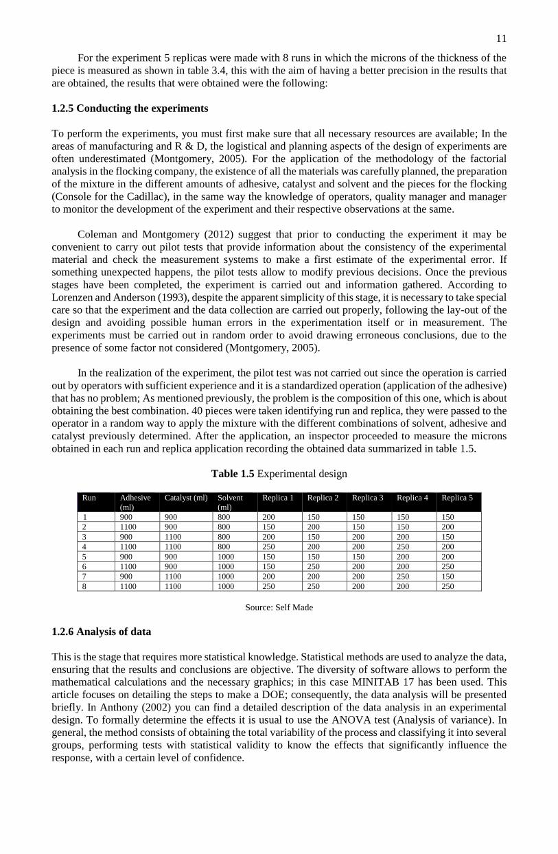
catalyst previously determined. After the application, an inspector proceeded to measure the microns

obtained in each run and replica application recording the obtained data summarized in table 1.5.

Table 1.5 Experimental design

Run Adhesive

(ml)

Catalyst (ml) Solvent

(ml)

Replica 1 Replica 2 Replica 3 Replica 4 Replica 5

1 900 900 800 200 150 150 150 150

2 1100 900 800 150 200 150 150 200

3 900 1100 800 200 150 200 200 150

4 1100 1100 800 250 200 200 250 200

5 900 900 1000 150 150 150 200 200

6 1100 900 1000 150 250 200 200 250

7 900 1100 1000 200 200 200 250 150

8 1100 1100 1000 250 250 200 200 250

Source: Self Made

1.2.6 Analysis of data

This is the stage that requires more statistical knowledge. Statistical methods are used to analyze the data,

ensuring that the results and conclusions are objective. The diversity of software allows to perform the

mathematical calculations and the necessary graphics; in this case MINITAB 17 has been used. This

article focuses on detailing the steps to make a DOE; consequently, the data analysis will be presented

briefly. In Anthony (2002) you can find a detailed description of the data analysis in an experimental

design. To formally determine the effects it is usual to use the ANOVA test (Analysis of variance). In

general, the method consists of obtaining the total variability of the process and classifying it into several

groups, performing tests with statistical validity to know the effects that significantly influence the

response, with a certain level of confidence.

12

1.3 Results

Once the sampling is done, the necessary calculations are carried out with the help of Minitab, with this

Software it will facilitate the analysis of the results as well as save time in its preparation. For the

hypothesis test, an ANOVA test is carried out with the objective of identifying those factors or

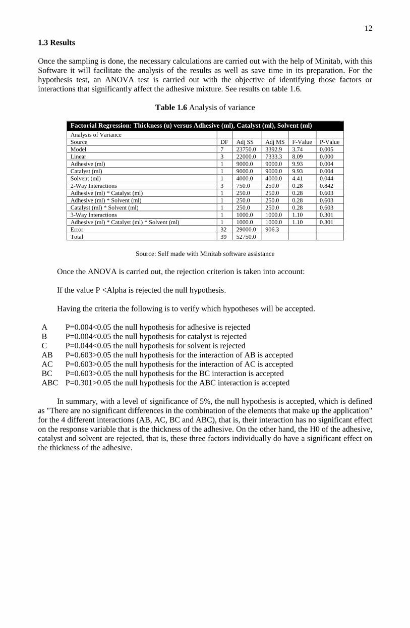
interactions that significantly affect the adhesive mixture. See results on table 1.6.

Table 1.6 Analysis of variance

Factorial Regression: Thickness (u) versus Adhesive (ml), Catalyst (ml), Solvent (ml)

Analysis of Variance

Source DF Adj SS Adj MS F-Value P-Value

Model 7 23750.0 3392.9 3.74 0.005

Linear 3 22000.0 7333.3 8.09 0.000

Adhesive (ml) 1 9000.0 9000.0 9.93 0.004

Catalyst (ml) 1 9000.0 9000.0 9.93 0.004

Solvent (ml) 1 4000.0 4000.0 4.41 0.044

2-Way Interactions 3 750.0 250.0 0.28 0.842

Adhesive (ml) * Catalyst (ml) 1 250.0 250.0 0.28 0.603

Adhesive (ml) * Solvent (ml) 1 250.0 250.0 0.28 0.603

Catalyst (ml) * Solvent (ml) 1 250.0 250.0 0.28 0.603

3-Way Interactions 1 1000.0 1000.0 1.10 0.301

Adhesive (ml) * Catalyst (ml) * Solvent (ml) 1 1000.0 1000.0 1.10 0.301

Error 32 29000.0 906.3

Total 39 52750.0

Source: Self made with Minitab software assistance

Once the ANOVA is carried out, the rejection criterion is taken into account:

If the value P <Alpha is rejected the null hypothesis.

Having the criteria the following is to verify which hypotheses will be accepted.

A P=0.004<0.05 the null hypothesis for adhesive is rejected

B P=0.004<0.05 the null hypothesis for catalyst is rejected

C P=0.044<0.05 the null hypothesis for solvent is rejected

AB P=0.603>0.05 the null hypothesis for the interaction of AB is accepted

AC P=0.603>0.05 the null hypothesis for the interaction of AC is accepted

BC P=0.603>0.05 the null hypothesis for the BC interaction is accepted

ABC P=0.301>0.05 the null hypothesis for the ABC interaction is accepted

In summary, with a level of significance of 5%, the null hypothesis is accepted, which is defined

as "There are no significant differences in the combination of the elements that make up the application"

for the 4 different interactions (AB, AC, BC and ABC), that is, their interaction has no significant effect

on the response variable that is the thickness of the adhesive. On the other hand, the H0 of the adhesive,

catalyst and solvent are rejected, that is, these three factors individually do have a significant effect on

the thickness of the adhesive.

13

Graphic 1.2 Pareto of standardized effects


We can see that Pareto's graphic 1.2 of standardized effects confirms that the three individual

factors A, B and C are those that have a significant effect since they cross the reference line that is in

2.037 and are statistically significant at the level of alpha 0.05.

Graphic 1.3 Waste Graphic


The 1.3 normal probability of effects graph is used to determine the magnitude, direction and

importance of the effects. In the normal probability of effects graph, the effects that are more distant from

0 are statistically significant, also show that the data follow a normal distribution and have a positive

standardized effect, that is, when the process changes from the low level to the level high of the factor,

the response is increased.

In the same graphic 1.3 the so-called "versus Fits" it is observed that the values are scattered,

indicating that they were obtained in a random way; since, as described by Box and Hunter (2005), the

randomization of the order of the experiments ensures, as far as possible, that any uncontrolled variable

(for example, laboratory temperature) contributes to the variability of repeatability and does not affect

the results systematically.

14

Once reviewed the graphs concentrated in the 1.4, the graphic of cube is elaborated where it is

possible to visualize the means of the realized runs, in this case it is necessary that the thickness of the

additive is between 150 to 250 microns, the data that I throw the graphic They are the following:

Graphic 1.4 Cube graphic


By looking at the graphic it is analyzed which is the best option we can take so that our thickness

is within what we request, so our average choice is 210 which is where the level of the adhesive and the

solvent is high but the level of the catalyst is low, showing that this mixture is optimal for the thickness

in the piece. Another way to check which mix is better is by means of the graphic 1.5 of intervals which

shows the means of the runs that were made.

Graphic 1.5 Thickness interval graphic


As seen in the previous graphic in the third interval we obtain that the type of mixture of each

component must be 1100 ml for the adhesive, 900 ml for the catalyst and 1000 ml for the solvent. To

avoid rapid drying ie application of between 50 and 60 sec.

15

1.4 Conclusions

The design of experiments is a technique that can help to know a process, it allows to find out how

various factors present in it influence the response and adjust them in the levels that optimize the results.

The objective of this article was to implement the DOE in a manufacturing process as part of the efforts

of innovation and application of statistics in a real environment that results in an improvement through

the application and verification of the usefulness of these tools. The seven steps proposed by

Montgomery for the realization of an experiment, in its practical application to the case of optimization

of the flocking process was a success.

In this case, through the realization of the experiments, the DOE technique allowed to determine

that the factors A (adhesive), B (catalyst) and C (solvent) are the most significant to optimize the flocking

of the pieces, that the three mentioned factors interact with each other, the other factors do not influence

significantly and you can work at the most convenient levels.

The DoE allows designs and analysis with more factors than the one presented in this case, since

in practical cases there are a number of variables to control. The planning of the experimentation, that

includes the stages of selection of factors, levels, answer and the own election of the most advisable

design, can be complicated in the practice; this makes it necessary to have a detailed methodology that

helps and facilitates the development of each stage. The results obtained after implementing the

corrective actions of the application of adhesive were favorable, since it was decreasing the pieces with

lack of flock to obtain consistently the required thickness of 210 microns. With this it was possible to

discard other variables such as temperature, calibration of the equipment, drying time, flock roughness

and flock with high electrical conductivity.

In conclusion, it is important that each operation that adds value to the product has a procedure

which indicates how it should be carried out, considering that if this is not carried out properly it will

have consequences once the product is finished, in the same way it is important that the quality

department has the appropriate information of what are the restrictions that a piece must meet so that it

is accepted without any defect and thus avoid a claim from the client, however, controlling the variables

that may affect the production will prevent them from being generated defects in the piece that occurs.

Engaging in the work method is highly recommended, because you can identify the different

variables that affect the flow of the process and the quality of products and / or services, whether by

labor, machinery or the environment, where there are regularly causes that cause these problems; It is

worth noting that finding the root cause of a problem using quality tools can be simple or complicated to

identify and solve, but thanks to the quality tools used in this case, such as the Ishikawa, AMEF and DOE

diagram, several alternatives can be proposed for solve the problems in the industry.

The methodology used confirms that statistical techniques have application for solving real

problems; through the analysis, management and treatment of data that involves the use of models that

combine the variables that alter the response result to improve the expected quality of the products and /

or services. By guaranteeing the correct thickness of the mixture, a flock adhesion of 0.9mm of uniform

height was ensured in the flocked parts, thus complying with the customer's specifications; since, as

described by Adams and Peppiat (1994), the classic elastic analysis predicts that the force increases with

the adhesive and attribute the bond strength to the micrometric thickness. In addition, Crocombe (1999)

explains that, if the adhesive becomes thicker, the plastic adhesion extension increases.

16

1.5 Annex 1 (Analysis of the Mode and Effect of Failure of the process of Flocking of automotive

parts)

Analysis of the mode and effect of the failure (amef of the process)

Name of the piece: Inner retrainer LHD/RHD Part

number:

116904543, 16905993 AMEF N°:

023

Type: SERIES

Process: Flocking of parts without pre-treatment Model (s) / Program: W168 Año (s): 2017 System ( ) Subsystem ( ) Component

(*)

Process manager: Production OEM (Fabricante): Tier 1 Client: XYZ Team members:

Drawing Level of

change:

NOT AVIABLE / REF FROM MAY

2009

Date of the AMEF: 17-MARCH-

17

Revision date: 22-DEC-17 Target Date:

Supplier no: - Other: Prepared by: Reviewed by:

Feature /

Process

System

Request Potenti

al

failure

mode

Potentia

l effect

(s) of

the fault

Sev

erit

y

Cla

ssif

icat

ion

Potentia

l cause

(s) of

the fault

Idea

Current status of controls in process

Det

ecti

on (

D)

NP

R

SxO

Resultados de acciones Actions

taken and

effective

date

S O D NPR

Prevention (P) Detection

(D)

Recommend

ed actions

Responsibl

e and date

of

completion

(30)

Adhesive

application

Correct

application

of adhesive

on the plastic

part

Excess

adhesiv

e

Parts

rejected

by rough

appearan

ce (AEP,

AGP)

6

Pot

pressure

paramete

r out of

standard

4

Pot pressure check, visual

verification of the piece

with adhesive before

going to the next process -

Autocontrol- (IT2.5 / 23)

Revision of the

piece with

adhesive

before starting

the flock

application

(IT2.5 / 23)

7 168 24

Parts

rejected

by rough

appearan

ce (AEP,

AGP)

6

Error in

the

applicati

on angle

4

Visual verification of the

piece with adhesive

before going to the next

process - Self-control-

(IT2.5 / 23) Application

adhesive training FM3.0 /

01

Revision of the

piece with

adhesive

before starting

the flock

application

(IT2.5 / 23)

7 168 24

Parts

rejected

by

adhesive

clumps

(EGA)

6

High

dosage of

air and /

or

adhesive

3


piece with adhesive





01

Revision of the

piece with

adhesive

before starting

the flock

application

(IT2.5 / 23)

7 128 18

Lack of

adhesive

Parts

rejected

due to

lack of

adhesive

in the

required

flock area

(ELF)

6 *

Does not

apply

adhesive

in

required

area

4


piece with adhesive





01

Revision of the

piece with

adhesive

before starting

the flock

application

(IT2.5 / 23)

7 168 24

Update the

sequence of

the adhesive

application

Update of

IT2.5 / 23 8 3 7 126

Thick

adhesive

thickness

Parts

rejected

by thin

adhesive

that

causes

low flock

density

(EFF)

6

Error in

the

applicati

on angle

4


piece with adhesive





01

Revision of the

piece with

adhesive

before starting

the flock

application

(IT2.5 / 23)

7 168 24

Little

adhesion

of fibers

Parts

rejected

by flock

with little

penetrati

on

(adhesion

) causing

low flock

density

(EFF)

6

Adhesive

drying in

the piece

due to

weather

or

waiting

time

4

Maintain maximum 2

pieces on the transit table

before flocking (IT2.5 /

23)

Revision of the

piece with

adhesive

before starting

the flock

application

(IT2.5 / 23)

7 168 24

Exceeded

flock

limits

Flock in

places

where it

is not

allowed

(ELF)

6 *

Failure to

apply

adhesive

4


piece with adhesive


process -Autocontrol-

(IT2.5 / 23)

Revision of the

piece with

adhesive

before starting

the flock

application

(IT2.5 / 23)

7 168 24

Areas of

the piece

without

adhesive

Areas of

the piece

without

flock

(EFF,

ELF)

6 *

Failure to

apply

adhesive

4


piece with adhesive


process -Autocontrol-

(IT2.5 / 23)

Revision of the

piece with

adhesive

before starting

the flock

application

(IT2.5 / 23)

7 168 24

Correct

application

of adhesive

Delay in

baking,

repetitio

n of

baking

Parts

without

correct

baking

(APF)

6

Failure to

prepare

the

adhesive

4 Verificar la preparación

de adhesivo (TI2.5/02)

Checking the

correct baking

of the piece

before starting

the cleaning

(IT2.5 / 23)

7 168 24

17

1.6 References

Adams RD, Peppiatt NA. Stress analysis of adhesively bonded lap joints. J Strain Analysis Eng

1994;9:185.

Antony, J. (2002). "Training for Design of Experiments Using a Catapult". Quality and

ReliabilityEngineering Intemational, Vol. 18, pp. 29-35

Box, G. E. P, Bisgaard, S. and Fung, C. (1988). "An Explanation and Critique of Taguchi's Contributions

to Quality Engineering". Quality and Reliability Engineering International, Vol. 4, pp. 123-131.

Cervantes, M J. and Engstrom, T. F. (2004). "Factorial Design Applied to CFD" . Joumal of Fluids

Engineenring. Asme, Vol. 126 (5), pp 791-798.

Chen, L.-H., & Ko, W.-C. (2009). Fuzzy linear programming models for new product design using QFD

with FMEA. Applied Mathematical Modelling, 33(2), 633–647.

Coleman, D. E. and Montgomery, D. C, (2012). "A Systematic Approach to Planning for a Designed

Industrial Experiment”. Technometrics, Vol. 35 (1), pp. 1-12.

Correa Espinal, A., & Medina Varela, P., & Velez Jaramillo, S. (2011). Mejoramiento del proceso de

manufactura de poleas para hornos rotatorios: Un enfoque desde el diseño Experimental. Scientia Et

Technica, XVI (48), 35-40.

Crocombe A.D. Global yielding as a failure criterion for bonded joints. International Journal for

Adhesion &Adhesives 1999; 9(3):145-53.

Drain, D. (1997). Handbook of Experimental Methods for Process Improvement, Ed. T. Science, 317.

George E. P. Box, J. Stuart Hunter, William G. Hunter (2005). Statistics for Experimenters: Design,

Innovation, and Discovery, 2nd EditionJohn Wiley & Sons

G. E. P and Behnken, D. W (2012). "Some New Three Level Design for the Study of Quantitative

Variables". Technometrics, Vol. 2 (4), pp. 455-475.

Kackar, R. N. (1989). "Off - Line Quality Control, Parameter Design and the Taguchi Method". Journal

of QualityTechnology, VoL 17 (4), pp. 176-188.

Lorenzen, T.J. and Anderson, V. L. (1993). Design of Experiments - A No-Name Approach, ed. Dekker.

414.

Melo, O., & Falla, C., & Jiménez, J. (2015). Efecto de datos influyentes en el análisis de diseños

factoriales de efectos fijos 3w. Ingeniería y Ciencia, 11 (22), 121-150.

Montgomery, D. C. (2005). Design and Analysis of Experiments. 6 ed. John Wiley & Sons.

Myers, R. H. and Montgomery, D. C. (2002). Response Surface Methodology. 2° Edición. W.

Interscience.

Pande, P S., Neuman, R. P and Cavanagh, R. R. (2000). The Six Sigma Way: How GE, Motorola, and

Other Top Companies are honnig their perfomance. Mc Graw Hill.

Pillay, A., & Wang, J. (2003). Modified failure mode and effects analysis using approximate reasoning.

Reliability Engineering & System Safety, 79(1), 69–85.

Plackett, R. L. and Burman, J. P (1946). "The Design of Optimum Multifactorial Experiments".

Biometrika, Vol. 33, pp. 305-325.

Chapter 1 Implementation of a 2k factorial design in the ...

Documents