Chaos in Power Electronics: An Overviecktse/pdf-paper/WS-chap16.pdf · Chaos in Power Electronics: An Overview ... ‡Department of Electronic and Information ... including power

16Chaos in Power Electronics: An Overview

Mario di Bernardo† and Chi K. Tse‡ 1

†Facolta di Ingegneria

Universita del Sannio in Benevento

82100 Benevento, Italy

(on leave from Dept. Eng. Maths,

University of Bristol, U.K.)

[email protected]

‡Department of Electronic and Information Engineering

The Hong Kong Polytechnic University

Hong Kong, China

[email protected]

Abstract

Power electronics is rich in nonlinear dynamics. Its operation ischaracterized by cyclic switching of circuit topologies, which givesrise to a variety of nonlinear behavior. This chapter provides anoverview of the chaotic dynamics and bifurcation scenarios observedin power electronics circuits, emphasizing the salient features of thecircuit operation and the modelling strategies. This chapter coversthe modelling approaches, analysis methods, and a classification ofthe common types of bifurcations observed in power electronics.

1Financial support for C.K. Tse to undertake this work has been provided by the HongKong Research Grants Council under Grant PolyU-5131/99E.

317

318 Chaos in Power Electronics

16.1 Introduction

Power electronics is a discipline spawned by real-life applications in industrial,commercial, residential and aerospace environments. Much of the developmentof the field of power electronics evolves around some immediate needs for solvingspecific power conversion problems. In the past three decades, power electron-ics has gone through intense development in many aspects of technology [1],including power devices, control methods, circuit design, computer-aided anal-ysis, passive components, packaging techniques, etc. Moreover, the principalfocus in power electronics, as reflected from topics discussed in some key powerelectronics conferences [2, 3], is to fulfill the functional requirements of theapplication for which the concerned circuits are used. Like many areas of engi-neering, power electronics is mainly motivated by practical applications, and itoften turns out that a particular circuit topology or system implementation hasfound widespread applications long before it is thoroughly analyzed and mostof its subtleties uncovered. For instance, the widespread application of a simpleswitching converter may date back to more than three decades ago. However,good analytical models allowing better understanding and systematic circuitdesign were only developed in late 1970’s [4], and in-depth analytical and mod-elling work is still being actively pursued today. Nonlinear phenomena, despitebeing commonly found in power electronics circuits, have only received formaltreatments in very recent years.

In this chapter, we review some of the nonlinear phenomena observed intypical power electronics systems. Our aim is to give an account of methodsand techniques that can be applied to study the many “strange” phenomenapreviously observed in power electronics. Simple dc/dc converters are used asrepresentative examples to illustrate the modelling approaches that are capa-ble of retaining the essential qualitative properties. Such properties, peculiarto switching and non-smooth systems, are systematically analyzed in terms ofpossible bifurcation scenarios and nonlinear phenomena. Our intention is toprovide an overview of the recent research efforts in the study of nonlinearphenomena in power electronics, and to summarize the essential analytical ap-proaches that can be used to perform a systematic classification of the nonlinearbehavior of power electronics systems. Since we wish to limit ourselves to aconcise overview of the main results, we will ignore the analytical details andsimply refer the readers to the main references listed at the end of the chapter.The rest of the chapter is outlined as follows. We begin in Sec. 16.2 with abrief overview of power electronics circuits, followed by a review of the classicalmethods of analysis in Sec. 16.3 and a discussion of the benefits of studyingchaotic dynamics in power electronics in Sec. 16.4. A quick tour of some recentfindings is presented in Sec. 16.5. In Secs. 16.6 and 16.7, we present a detaileddiscussion of the modelling methods for characterizing nonlinear phenomena

Power Electronics Circuits: A Brief Overview 319

+

−

S

DVin

L

C Vo

+

−

(a)

+

−

S

VinC Vo

−

+

(b)

+

−VinC Vo

+

−

(c)

L

D

S

L

D

FIGURE 16.1Simple dc/dc converters. (a) Buck converter; (b) buck-boost converter; (c)boost converter.

such as bifurcation and chaos in power electronics.

16.2 Power Electronics Circuits: A Brief Overview

Regardless of its specific function, a power electronics circuit operates by tog-gling its topology among a set of linear or nonlinear circuit topologies, underthe control of a feedback system. As such, they can be regarded as piecewise-switched circuits.

For example, in simple dc/dc converters, such as the ones shown in Fig. 16.1,an inductor is ‘switched’ between the input and the output through an appro-priate switching element (labelled as S in the figure). The way in which theinductor is switched determines the output voltage level and transient behav-ior. Usually, a semiconductor switch and a diode are used to implement thesaid switching, and through the use of a feedback control circuit, the relativedurations of the various switching intervals can be continuously adjusted. Suchfeedback action effectively controls the dynamics and steady-state behavior ofthe circuit. Thus, both the circuit topology and the control method determinesthe dynamical behavior of a power electronics circuit.


16.2.1 Simple DC/DC converters

Many power electronics converters are constructed on the basis of the threesimple converters shown in Fig. 16.1. In a typical period-1 operation, theswitch S and the diode D are turned on and off in a cyclic and complementaryfashion, under the command of a pulse-width modulator. When the switchS is closed (the diode D is open), the inductor current ramps up. When theswitch S is open (the diode D closed), the inductor current ramps down. Theduty ratio, defined as the fraction of a repetition period during which S isclosed, is continuously controlled by a feedback circuit that aims to maintainthe output voltage at a fixed level even under input and load variations. Twotypical feedback arrangements are shown in the next subsection.

The behavior of a dc/dc converter is greatly influenced by its operating mode.Typically, we can distinguish two different modes of operation, namely, con-tinuous conduction mode (CCM) and discontinuous conduction mode (DCM).In CCM, the inductor current is maintained non-zero throughout the entirerepetition cycle. This happens when the inductance L is relatively large, orthe load current demand is relatively high. Moreover, in DCM, the inductorcurrent is zero for an interval of time within a cycle. This happens when theinductance L is relatively small, or the load current demand is low, causing theinductor current to fall to zero as the inductor is being discharged. During theinterval of zero inductor current, both switch S and diode D are open.

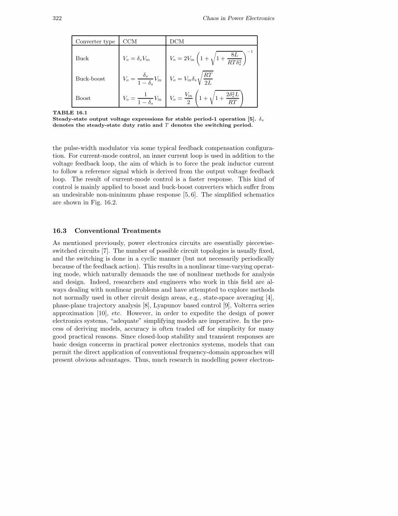
For both CCM and DCM, the output voltage has a fixed relationship withthe input voltage, as determined by the duty ratio. A steady-state relationshipcan be easily found from a volt-time balance consideration of the inductor.Table 16.1 shows the steady-state output voltage expressions for stable period-1 operation [5]. Here, we denote by δs the steady-state duty ratio, and by Tthe repetition period.

As we will see in this chapter, although the period-1 stable operation is thepreferred operation for most industrial applications, it represents only one par-ticular operating regime. Because of the existence of many possible operatingregimes, it would be of practical importance to have a thorough understandingof what determines the behavior of the circuit so as to guarantee a desiredoperation or to avoid an undesirable one.

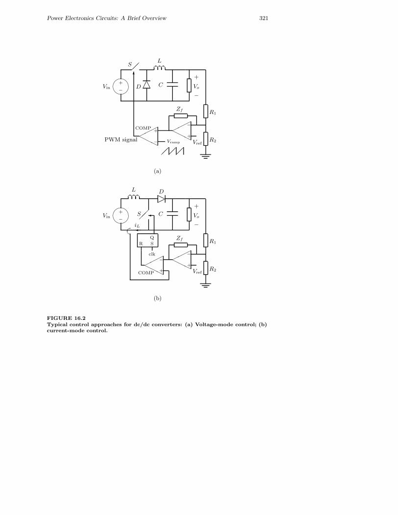
16.2.2 Typical control strategies

Most dc/dc converters are designed to deliver a regulated output voltage. Thecontrol of dc/dc converters usually takes on two approaches, namely voltagefeedback control and current-programmed control, also known as voltage-modeand current-mode control, respectively [6]. In voltage-mode control, the outputvoltage is compared with a reference to generate a control signal which drives

Power Electronics Circuits: A Brief Overview 321

+

−

S

DVin

L

C Vo

+

−

(a)

+

−VinC Vo

+

−

(b)

L

D

S

−

+

+

−

Zf R1

R2Vref

Vramp

R1

R2

+

−

Zf

Vref

+

−

R S

Q

clk

PWM signal

COMP

COMP

iL

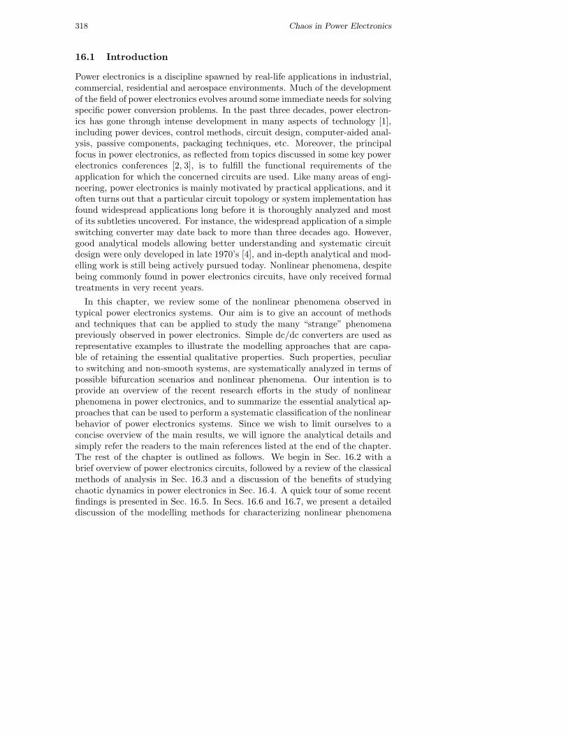
FIGURE 16.2Typical control approaches for dc/dc converters: (a) Voltage-mode control; (b)current-mode control.


Converter type CCM DCM

Buck Vo = δsVin Vo = 2Vin

(1 +

√1 +

8L

RTδ2s

)−1

Buck-boost Vo =δs

1 − δsVin Vo = Vinδs

√RT

2L

Boost Vo =1

1 − δsVin Vo =

Vin

2

(1 +

√1 +

2δ2sL

RT

)

TABLE 16.1Steady-state output voltage expressions for stable period-1 operation [5]. δs

denotes the steady-state duty ratio and T denotes the switching period.

the pulse-width modulator via some typical feedback compensation configura-tion. For current-mode control, an inner current loop is used in addition to thevoltage feedback loop, the aim of which is to force the peak inductor currentto follow a reference signal which is derived from the output voltage feedbackloop. The result of current-mode control is a faster response. This kind ofcontrol is mainly applied to boost and buck-boost converters which suffer froman undesirable non-minimum phase response [5, 6]. The simplified schematicsare shown in Fig. 16.2.

16.3 Conventional Treatments

As mentioned previously, power electronics circuits are essentially piecewise-switched circuits [7]. The number of possible circuit topologies is usually fixed,and the switching is done in a cyclic manner (but not necessarily periodicallybecause of the feedback action). This results in a nonlinear time-varying operat-ing mode, which naturally demands the use of nonlinear methods for analysisand design. Indeed, researchers and engineers who work in this field are al-ways dealing with nonlinear problems and have attempted to explore methodsnot normally used in other circuit design areas, e.g., state-space averaging [4],phase-plane trajectory analysis [8], Lyapunov based control [9], Volterra seriesapproximation [10], etc. However, in order to expedite the design of powerelectronics systems, “adequate” simplifying models are imperative. In the pro-cess of deriving models, accuracy is often traded off for simplicity for manygood practical reasons. Since closed-loop stability and transient responses arebasic design concerns in practical power electronics systems, models that canpermit the direct application of conventional frequency-domain approaches willpresent obvious advantages. Thus, much research in modelling power electron-

Bifurcations and Chaos in Power Electronics 323

ics circuits has been directed towards the derivation of a linear model that isappropriate to a frequency-domain analysis; the limited validity being the priceto pay. (The fact that most engineers are trained to use linear methods is alsoa strong motivation for developing linearized models.) For example, the aver-aging approach [4], one of the most widely adopted modelling approaches forswitching converters, initially yields simple nonlinear models that contain notime-varying parameters and hence can be used more conveniently for analysisand design. Essentially, an averaged model discards the switching details andfocuses only on the envelope of the dynamical motion. This is well suited tocharacterize power electronics circuits in the low-frequency domain.

In practice, moreover, such so-called “averaged” models are often linearizedto yield linear time-invariant models that can be directly studied in a standardLaplace transform domain or frequency domain, facilitating design of controlloops and evaluation of transient responses in ways that are familiar to practi-tioners.

16.4 Bifurcations and Chaos in Power Electronics

Power electronics engineers frequently encounter such phenomena as subhar-monic oscillations, jumps, quasi-periodic operations, sudden broadening ofpower spectra, bifurcations and chaos, despite not knowing what causes them[11, 12]. Most power supply engineers would have experienced bifurcation phe-nomena and chaos in switching regulators when some parameters (e.g., inputvoltage and feedback gain) are varied, but usually do not examine the phenom-ena in detail. The usual reaction of the engineers is to avoid these phenomenaby adjusting component values and parameters, often through some trial-and-error procedure. Thus, the phenomena remain somewhat mysterious and rarelyexamined in a formal manner.

What has been said so far may be regarded as a kind of stereotypical de-velopment in application-driven disciplines. Indeed, if linear models can beprofitably used in design (and as long as the restricted validity of the mod-els does not adversely compromise the design integrity), there seems to be noimmediate needs for investigating such nonlinear phenomena as chaos and bi-furcation. However, as the field of power electronics gains maturity and as thedemand for better functionality, reliability and performance of power electron-ics systems increases, in-depth analysis into nonlinear behavior and phenomenabecomes justifiable and even mandatory. On the one hand, the study of nonlin-ear phenomena offers the opportunity of rationalizing the commonly observedbehavior. Thus, knowing how and when chaos occurs, for instance, will cer-tainly help avoid it, if “avoiding it” is what the engineers want. On the otherhand, many previously unused nonlinear operating regimes may be profitably


exploited for useful engineering applications, provided that such operations arethoroughly understood. For these reasons, the study of bifurcations and chaosin power electronics has recently attracted much attention from both the powerelectronics and the circuits and systems communities.

In the next section, we present a chronological survey of the recent findingsin the identification, analysis and modelling of nonlinear phenomena in powerelectronics circuits and systems.

16.5 A Survey of Research Findings

The occurrence of bifurcations and chaos in power electronics was first reportedin the literature in the late eighties by Hamill et al. [13, 14]. Experimentalobservations regarding boundedness, chattering and chaos were also made byKrein and Bass [15] back in 1990. Although these early reports did not containany rigorous analysis, they seriously pointed out the importance of studyingthe complex behavior of power electronics and its likely benefits for practicaldesign. Since then, much interest has been aroused in the power electronicsand circuits research communities in pursuing formal studies of the complexphenomena commonly observed in power electronics.

In 1990, Hamill et al. [16] presented a paper at the IEEE Power Electron-ics Specialists Conference, reporting an attempt to study chaos in a simplebuck converter which became a subject of intensive research in the follow-ing decade (and still is!). Using an implicit iterative map, the occurrenceof period-doublings, subharmonics and chaos in a simple buck converter wasdemonstrated by numerical analysis, PSPICE simulation and laboratory mea-surement. The derivation of a closed-form iterative map for the boost converterunder a current-mode control scheme was presented later by the same group ofresearchers [17]. This closed-form iterative map allowed the analysis and clas-sification of bifurcations and structural instabilities of this simple converter.Since then, a number of authors have contributed to the identification of bifur-cation patterns and strange attractors in a wider class of circuits and devices ofrelevance in power electronics. Some key publications are summarized below.See also [18–20] for alternative reviews.

The occurrence of period-doubling cascades for a simple dc/dc converteroperating in DCM was reported in 1994 by Tse [21, 22]. By modelling thedc/dc converter operating in DCM as a first-order iterative map, the onset ofperiod-doubling bifurcations can be located analytically. The idea is based onevaluating the Jacobian of the iterative map about the fixed point correspond-ing to the solution undergoing the period-doubling, determining the conditionfor which a period-doubling bifurcation occurs (i.e., Jacobian equals −1). Sim-ulations and laboratory measurements have confirmed the findings. Formal

A Survey of Research Findings 325

0.2

0.3

0.4

0.5

0.6

0.7

0.8

0.9

1

0.4 0.5 0.6 0.7 0.8 0.9 1

i

Iref

0.1

0.2

0.3

0.4

0.5

0.6

0.7

0.8

0.9

1

1.1

1.2

0.3 0.4 0.5 0.6 0.7 0.8 0.9 1 1.1 1.2

i

Iref

(a) (b)

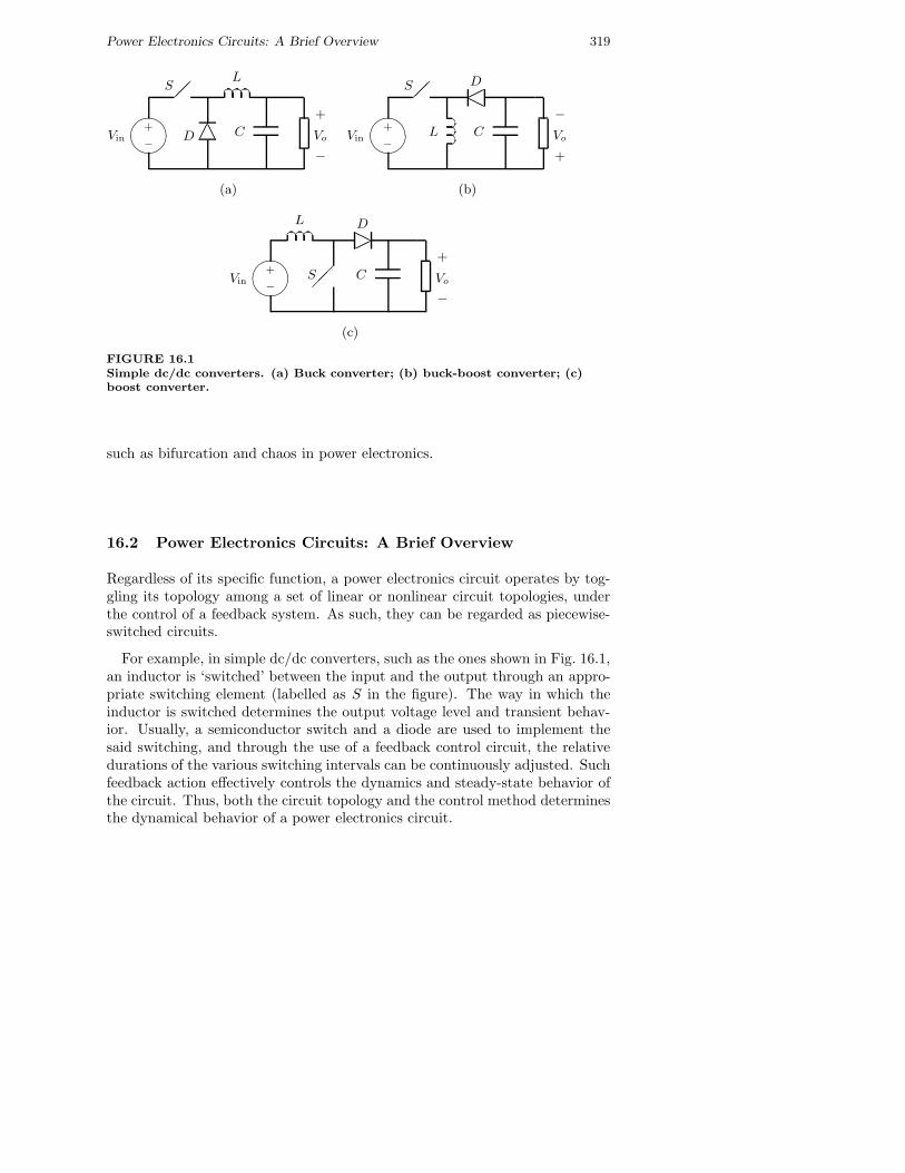
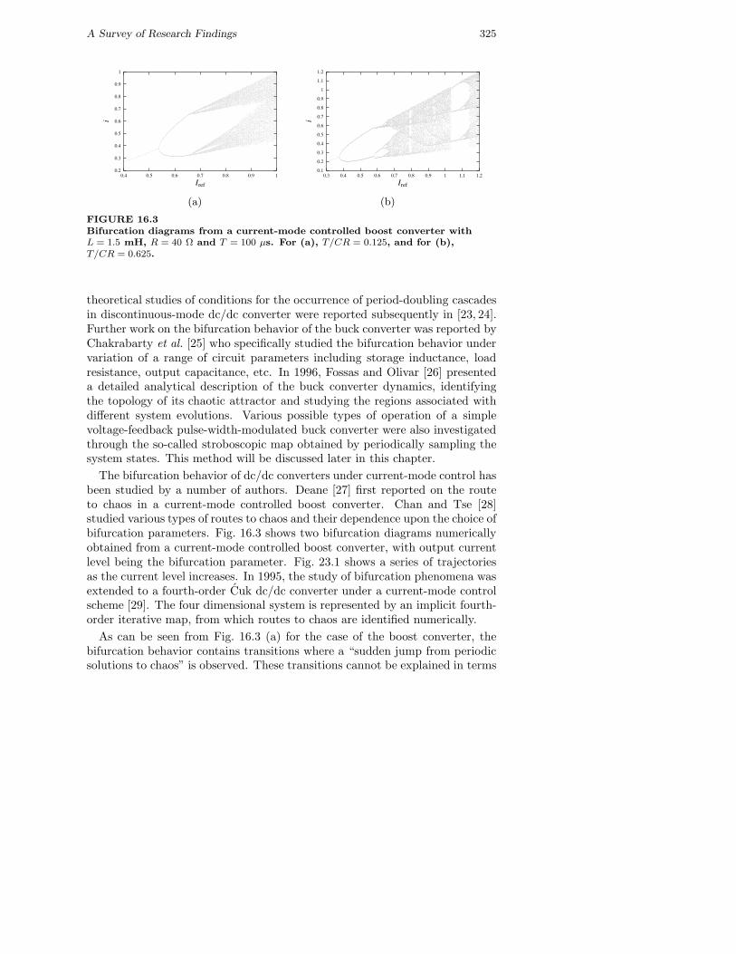
FIGURE 16.3Bifurcation diagrams from a current-mode controlled boost converter withL = 1.5 mH, R = 40 Ω and T = 100 µs. For (a), T/CR = 0.125, and for (b),T/CR = 0.625.

theoretical studies of conditions for the occurrence of period-doubling cascadesin discontinuous-mode dc/dc converter were reported subsequently in [23, 24].Further work on the bifurcation behavior of the buck converter was reported byChakrabarty et al. [25] who specifically studied the bifurcation behavior undervariation of a range of circuit parameters including storage inductance, loadresistance, output capacitance, etc. In 1996, Fossas and Olivar [26] presenteda detailed analytical description of the buck converter dynamics, identifyingthe topology of its chaotic attractor and studying the regions associated withdifferent system evolutions. Various possible types of operation of a simplevoltage-feedback pulse-width-modulated buck converter were also investigatedthrough the so-called stroboscopic map obtained by periodically sampling thesystem states. This method will be discussed later in this chapter.

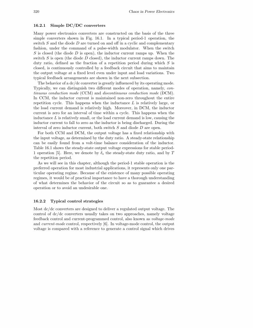
The bifurcation behavior of dc/dc converters under current-mode control hasbeen studied by a number of authors. Deane [27] first reported on the routeto chaos in a current-mode controlled boost converter. Chan and Tse [28]studied various types of routes to chaos and their dependence upon the choice ofbifurcation parameters. Fig. 16.3 shows two bifurcation diagrams numericallyobtained from a current-mode controlled boost converter, with output currentlevel being the bifurcation parameter. Fig. 23.1 shows a series of trajectoriesas the current level increases. In 1995, the study of bifurcation phenomena wasextended to a fourth-order Cuk dc/dc converter under a current-mode controlscheme [29]. The four dimensional system is represented by an implicit fourth-order iterative map, from which routes to chaos are identified numerically.

As can be seen from Fig. 16.3 (a) for the case of the boost converter, thebifurcation behavior contains transitions where a “sudden jump from periodicsolutions to chaos” is observed. These transitions cannot be explained in terms


6.2

6.4

6.6

6.8

7

7.2

7.4

7.6

7.8

0.18 0.2 0.22 0.24 0.26 0.28 0.3

v

i

6

6.5

7

7.5

8

8.5

9

9.5

10

10.5

0.2 0.25 0.3 0.35 0.4 0.45 0.5

v

i

(a) (b)

6

7

8

9

10

11

12

0.2 0.25 0.3 0.35 0.4 0.45 0.5 0.55 0.6

v

i

5

6

7

8

9

10

11

12

13

14

15

16

0.2 0.3 0.4 0.5 0.6 0.7 0.8

v

i

(c) (d)

FIGURE 16.4Trajectories from a current-mode controlled boost converter. (a) Stableperiod-1 operation; (b) stable period-2 operation; (c) stable period-4 operation;and (d) chaotic operation.

of standard bifurcations such as “period-doubling” and “saddle-node”. In fact,as studied by Banerjee et al. [30, 31] and Di Bernardo [32], these transitionsare due to a novel class of bifurcation known as “grazing” or “border-collision”bifurcation, which is unique to switched dynamical systems [33–35].

Since most power electronics circuits are non-autonomous systems driven byfixed-period clock signals, the study of the dynamics can be effectively carriedout using appropriate discrete-time maps. In addition to the aforementionedstroboscopic maps (which will be discussed in the next section), Di Bernardoet al. [24] studied alternative sampling schemes and their applications to thestudy of bifurcation and chaos in power electronics [32]. It has been foundthat non-uniform sampling can be used to derive discrete-time maps (termedA-switching maps) which can be used to effectively characterize the occurrenceof bifurcations and chaos in both autonomous and non-autonomous systems.These maps turned out to be particularly useful for the investigation of non-smooth bifurcation in power electronics circuits and systems. Also, the occur-rence of periodic chattering was explained in terms of sliding solutions [36].

Modelling Strategies 327

When external clocks are absent and the system is “free-running”, for ex-ample, under a hysteretic control scheme, the system is autonomous and doesnot have a fixed switching period. Such free-running converters were indeedextremely common in the old days when fixed-period integrated-circuit con-trollers were not available. For this type of autonomous converters, chaos can-not occur if the system order is below three. A representative example is thefree-running Cuk converter which has been shown by Tse et al. [37] to exhibitHopf bifurcation and chaos.

Power electronics circuits other than dc/dc converters have also been exam-ined in recent years. Dobson et al. [38] reported “switching time bifurcation”of diode and thyristor circuits. Such bifurcation manifests as jumps in theswitching times. Bifurcation phenomena from induction motor drives were re-ported separately by Kuroe [39] and Nagy et al. [40]. Finally, some attemptshave been made to study higher order parallel-connected systems of converterswhich are becoming popular design choice for high current applications [41].

16.6 Modelling Strategies

In Sec. 16.3, we discussed the conventional “averaging” method for modellingpower electronics circuits. In essence, averaging retains the low-frequency prop-erties while ignoring the detailed dynamics within a switching cycle. Usually,the validity of averaged models is only restricted to the low-frequency rangeup to an order of magnitude below the switching frequency. For this reason,averaged models become inadequate when the aim is to explore nonlinear phe-nomena that may appear across a wide spectrum of frequencies. Nevertheless,averaging techniques can be useful to analyze those bifurcation phenomenawhich are confined to the low-frequency range. For instance, in a free-runningCuk converter, Hopf bifurcation that gives birth to a limit cycle consisting ofmany switching periods (low-frequency behavior) can be clearly observed froma suitable averaged model [37].

An effective approach for modelling power electronics circuits with a high de-gree of exactness is to use appropriate discrete-time maps obtained by uniformor non-uniform sampling of the system states. Essentially the aim is to derivean iterative function that expresses the state variables at one sampling instantin terms of those at an earlier sampling instant. In what follows, the basicconcepts of discrete-time maps and how they can be used to explore nonlinearphenomena in power electronics are explained.


16.6.1 Discrete-time maps

As is often the case in nonlinear dynamical systems, the analysis of complexphenomena that are of relevance to engineering requires “adequate” models. Asmentioned previously, discrete-time maps obtained by suitable sampling of thesystem dynamics can be extremely useful for characterizing the occurrence ofbifurcations and chaos in power electronics circuits. For the sake of clarity, wedistinguish two different classes of maps, namely Poincare maps and normal-form maps. The former is useful for describing the global dynamics of thesystem under investigation from one sampling instant to the next. The latter,which is valid locally to a bifurcation point, is an invaluable tool for classifyingthe system behavior following the onset of a bifurcation. In what follows wefocus on the derivation of appropriate Poincare maps for dc/dc converters. Theuse of normal-form maps for classification will be left to the next section.

Several kinds of Poincare maps have been defined for the analysis of non-linear phenomena in power electronics circuits. For convenience, we use avoltage-controlled buck converter as an representative example to illustrate thederivation of the most commonly used maps, namely, the stroboscopic map, theS-switching (synchronous switching) map, and the A-switching (asynchronousswitching) map.

Specifically the buck converter can be described by a piecewise smooth sys-tem of the form:

di(t)dt

= − 1L

v(t) +δ(t)L

E,

dv(t)dt

=1C

i(t) − 1RC

v(t),

(16.6.1)

where i(t) is the inductor current, v(t) the capacitor voltage, E a constant inputvoltage, and δ(t) a modulated signal which is 0 whenever a linear combinationof the system states, vc(t) = gii(t) + gvv(t), is greater than an appropriatelygenerated ramp signal of period T , vr(t) = γ + η(t mod T ), and is 1 otherwise(i.e., δ(t) is 0 when the switch is OFF, and is 1 when the switch is ON).

Without loss of generality, let us assume that the converter begins its evolu-tion at a time instant equal to an integral multiple of the modulating period,and that the converter assumes δ(t) = 1 initially. For brevity, we refer to thephase with δ(t) = 1 as phase 1, and to that with δ(t) = 0 as phase 2. Thus,the converter stays in phase 1 until the next commutation is reached, and soon.

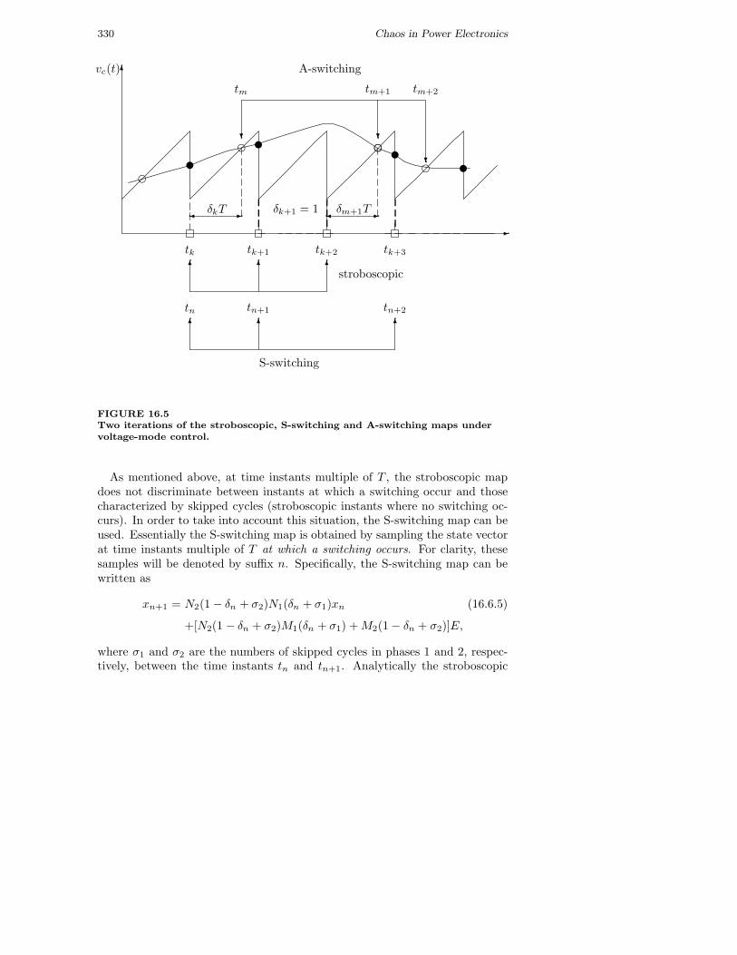
In general, discrete-time maps can be categorized into the following threeclasses (see Fig. 16.5).

• Stroboscopic map: obtained by sampling the system states periodicallyat time instants which are multiples of the period of the ramp signal vr


(stroboscopic instants). Note that the system states are sampled at eachstroboscopic instant irrespectively of whether the system configurationswitches or not at that instant.

• S-switching map (synchronous switching): obtained by sampling the sys-tem states at those stroboscopic time instants when the system commutesfrom phase 2 to phase 1.

• A-switching map (asynchronous switching): obtained by sampling thesystem states at time instants within each ramp cycle when the systemcommutes from phase 1 to phase 2.

In order to derive the relevant maps, we introduce the following two simpli-fying assumptions. These assumptions can be later removed.

1. No more than one commutation takes place during each period of themodulating signal.

2. The commutation from phase 2 to phase 1 can only take place at timeinstants which are multiples of the ramp cycle T .

Note that the second assumption is always true when the converter is undercurrent-mode control, but is not so for voltage-mode control.

16.6.2 Derivation of stroboscopic and S-switching maps

The stroboscopic map is the most widely used type of discrete-time maps formodelling dc/dc converters. It can be obtained by sampling the system dy-namics every T seconds, say, at the beginning of each ramp cycle. To avoidconfusing with other types of maps, we use suffix k as the counting index forthis map, as shown in Fig. 16.5. Applying a simple iterative procedure to thesolutions of the state equations for phases 1 and 2, the stroboscopic map canobtained as

xk+1 = N2(1 − δk)N1(δk)xk + [N2(1 − δk)M1(δk) + M2(1 − δk)] E, (16.6.2)

where xk denotes x(kT ), δk is the duty ratio in the kth period, and the solutionto the state equation in each phase is given by x(δ) = Ni(δ) + Mi(δ)E with

Ni(δ) = eAiδT (16.6.3)

Mi(δ) = A−1i (eAiδT − I)Bi. (16.6.4)

Moreover, under certain drastic control conditions, the converter may stay inphase 1 or phase 2 for the entire period. In such cases (normally called skippedcycles), one must assume δk = 1 or δk = 0, as appropriate.


vc(t)

tm+2tm

tk

tm+1

tk+1 tk+2

A-switching

tk+3

tn tn+1 tn+2

stroboscopic

S-switching

δkT δk+1 = 1

δm+1T

FIGURE 16.5Two iterations of the stroboscopic, S-switching and A-switching maps undervoltage-mode control.

As mentioned above, at time instants multiple of T , the stroboscopic mapdoes not discriminate between instants at which a switching occur and thosecharacterized by skipped cycles (stroboscopic instants where no switching oc-curs). In order to take into account this situation, the S-switching map can beused. Essentially the S-switching map is obtained by sampling the state vectorat time instants multiple of T at which a switching occurs. For clarity, thesesamples will be denoted by suffix n. Specifically, the S-switching map can bewritten as

xn+1 = N2(1 − δn + σ2)N1(δn + σ1)xn (16.6.5)

+[N2(1 − δn + σ2)M1(δn + σ1) + M2(1 − δn + σ2)]E,

where σ1 and σ2 are the numbers of skipped cycles in phases 1 and 2, respec-tively, between the time instants tn and tn+1. Analytically the stroboscopic


and the S-switching maps are identical when σ1 = 0 and σ2 = 0.In the open-loop case, i.e., gT = (0, 0), the stroboscopic map is linear. How-

ever, it becomes nonlinear when a closed-loop control is activated. This isbecause the duty ratio δn depends on the system states as a consequence ofintroducing the feedback control. Moreover, the construction of the map un-der closed-loop condition usually requires solving δn from a control equation,which is not necessarily in closed form. In fact, with the exception of current-mode controlled boost and buck-boost converters with zero inductance’s seriesresistance, the control equation involving δn is transcendental and can only besolved numerically. Therefore, under closed-loop condition, the stroboscopicand the S-switching maps cannot be written in closed form for most cases.

16.6.3 Derivation of A-switching maps

The A-switching map is obtained when the state vector is asynchronously sam-pled at switching times internal to the modulating period, as shown in Fig. 16.5.Specifically we can readily write down the A-switching map by noting that theconverter enters phase 2 after an A-switching, i.e.,

xm+1 = N1(δm+1 + σ1)N2(1 − δm + σ2)xm (16.6.6)

+[N1(δm+1 + σ1)M2(1 − δm + σ2) + M1(δm+1 + σ1)]E.

In order to construct the A-switching map under a closed-loop condition, thevariables δm+1 and δm must be eliminated from (16.6.6). To do this, we assumethat the following conditions are defined by the control law as the conditionsfor an A-switching:

gT xm = α + βδmT, (16.6.7)

gT xm+1 = α + βδm+1T. (16.6.8)

Let us assume that β = 0 for simplicity. This assumption will be laterremoved. By computing δm from (16.6.7) and δm+1 from (16.6.8), and puttingthem in (16.6.6), we obtain the following A-switching map for the closed-loopsystem:

xm+1 = N1(γT xm+1 − a + σ1)N2(1 − γT xm + a + σ2)xm

+[N1(γT xm+1 − a + σ1)M2(1 − γT xm + a + σ2)

+M1(γT xm+1 − a + σ1)]E, (16.6.9)

where γT = gT /(βT ) and a = α/(βT ). Note that (16.6.9) has a closed form,although it is an implicit map.


As detailed in [19], explicit functional forms can be used by consideringappropriate simplified maps. These can be obtained by using a small-signalapproximation, i.e., by Taylor-expanding the exponential functions which char-acterize the maps introduced above.

All the maps introduced above can be used to obtain analytical conditionsfor the existence of given periodic orbits and standard bifurcations such asperiod-doubling and saddle-node. Many reports of standard bifurcations, assurveyed earlier, have effectively employed the stroboscopic and S-switchingmaps [18–20]. Moreover, the A-switching maps are particularly useful for theanalysis of multi-switching behavior, and can be constructed more convenientlyfor operations where skipped cycles are frequent such as when the converter isoperating in a chaotic regime.

16.7 Analysis and Classification of Non-smooth Bifurcations

The literature already abounds with methods of analysis and classification ofstandard bifurcations like period-doubling and saddle-node [42]. In the follow-ing we focus on the non-smooth bifurcations, which are particularly relevantto power electronics.

16.7.1 System formulation

As discussed earlier, because of their switching nature, power electronics sys-tems are often modelled by sets of ordinary differential equations (ODEs) ormaps which are intrinsically piecewise-smooth (PWS). Specifically, wheneverthe circuit under investigation switches to a different configuration (for exam-ple, from ON to OFF, or vice versa), the vector field of the correspondingmodel changes from one functional form to another. Thus, mathematically,power electronics circuits can be modelled by dynamical systems of the form:

x =

F1(x, µ, t), ifx ∈ S1

F2(x, µ, t), ifx ∈ S2

. . .

Fk(x, µ, t), ifx ∈ Sk

(16.7.10)

where Fi : Rn+p+1 → Rn, i = 1, · · · , k, is smooth in each of the phase-spaceregions, Si, and µ is a system parameter. Also, the system switches from onefunctional form Fi to another Fj, whenever the system states move from regionSi to region Sj .

Along the boundaries between different regions, say Φi,j , the system statescan have different degrees of discontinuity. In particular, according to the

Analysis and Classification of Non-smooth Bifurcations 333

properties of the system along its discontinuity boundaries, we can identifythree main classes of PWS dynamical systems:

• Systems with discontinuous states (jumps);• Systems with a discontinuous vector field, i.e., the first derivative of the

system states is discontinuous across the phase-space boundaries;• Systems with a discontinuous Jacobian (i.e. Fix = Fjx), i.e., the second

derivative of the system states is discontinuous across the phase-spaceboundaries.

Moreover, the discontinuity boundaries between different phase-space regionscan themselves be smooth or piecewise smooth.

For example, consider the dc/dc buck converter depicted in Fig. 16.1 (a) anddescribed by (16.6.1). Suppose that the ramp signal vr defines a discontinuityboundary, Φ, which is itself discontinuous and divides the phase space into twoseparate regions associated with the ON and OFF configurations. In this case,the first derivative of the system states varies discontinuously as the boundaryΦ is crossed [36].

16.7.2 Bifurcation possibilities

Power electronics systems can exhibit standard bifurcations such as period-doubling or saddle-node. Such bifurcations are indeed frequently observed bothanalytically and experimentally, as surveyed earlier in Sec. 16.5. Nevertheless,some of the most common dynamical transitions observed in power electron-ics circuits, such as the “sudden jump to chaos” mentioned earlier, cannot beexplained in terms of standard bifurcations [43–45]. In fact, power electronicssystems, being switched dynamical systems, are known to exhibit an interestingclass of bifurcations which cannot be observed in their smooth counterparts.Specifically, for switched dynamical systems, a dramatic change of the systembehavior is usually observed when a part of the system trajectory hits tangen-tially one of the boundaries between different regions in phase space. Whenthis occurs, the system is said to undergo a grazing bifurcation which is alsoknown as C-bifurcation in the Russian literature [46–49].

For example, in the case of the buck converter, such an event correspondsto the feedback signal “grazing” the tip of the ramp signal at a stroboscopicpoint. As studied by Banerjee et al. [31] and shown further by Di Bernardo etal. [50], it is possible to analyze the system behavior associated with “grazing”by considering an appropriate piecewise linear normal-form map of the form:

xm+1 →

A1xm + Bµ, if the system is in phase 1A2xm + Bµ, if the system is in phase 2

(16.7.11)


M0

S

D

D

−

+

Γ

x n

L0

L-

M

M

*

**

Φ0

L+

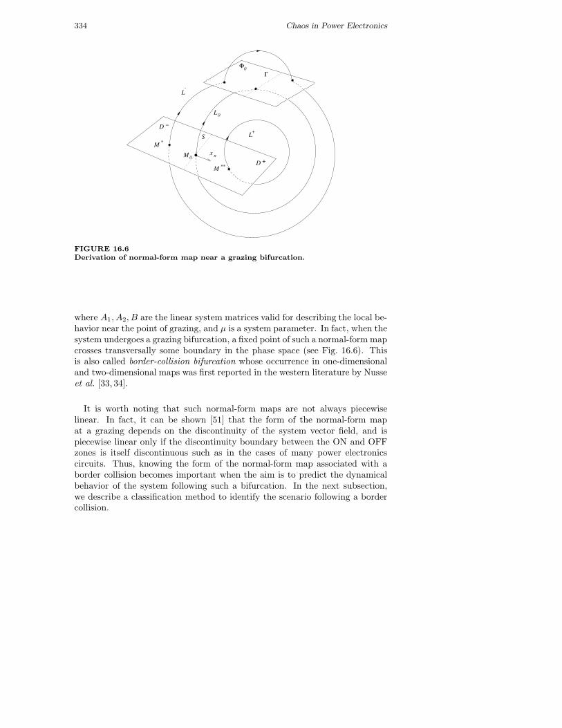
FIGURE 16.6Derivation of normal-form map near a grazing bifurcation.

where A1, A2, B are the linear system matrices valid for describing the local be-havior near the point of grazing, and µ is a system parameter. In fact, when thesystem undergoes a grazing bifurcation, a fixed point of such a normal-form mapcrosses transversally some boundary in the phase space (see Fig. 16.6). Thisis also called border-collision bifurcation whose occurrence in one-dimensionaland two-dimensional maps was first reported in the western literature by Nusseet al. [33, 34].

It is worth noting that such normal-form maps are not always piecewiselinear. In fact, it can be shown [51] that the form of the normal-form mapat a grazing depends on the discontinuity of the system vector field, and ispiecewise linear only if the discontinuity boundary between the ON and OFFzones is itself discontinuous such as in the cases of many power electronicscircuits. Thus, knowing the form of the normal-form map associated with aborder collision becomes important when the aim is to predict the dynamicalbehavior of the system following such a bifurcation. In the next subsection,we describe a classification method to identify the scenario following a bordercollision.

Analysis and Classification of Non-smooth Bifurcations 335

16.7.3 Classification

We begin with a brief description of the derivation of the normal-form map as-sociated with a grazing or border-collision bifurcation. Referring to Fig. 16.6,suppose that as the value of some parameter µ increases, a periodic orbit of sys-tem (16.7.10), say L0, becomes tangent (grazing) to the switching hyperplane,Φ0, when µ = µ. The grazing limit cycle L0 is associated with a fixed point, sayM0, on the Poincare section D. As the parameter µ is varied, such a fixed pointmoves from M∗ to M∗∗, i.e., from a fixed point associated with an orbit whichdoes not cross the boundary to one corresponding to a solution which crossesthe boundary. Linearizing the system flow about each of these fixed points, wecan then obtain a piecewise linear map of the form (16.7.11). This approximatemap is valid if the switching hyperplane Φ0 is itself non-smooth [51].

An effective method for classifying and predicting the dynamical scenariosfollowing a border-collision bifurcation is given in Di Bernardo et al. [52]. Theavailable results (up to now) for the n-dimensional case are summarized asfollows. Let σ+

1 and σ+2 be the numbers of eigenvalues, respectively, of A1

and A2 in (16.7.11), which are greater than 1. Likewise, let σ−1 and σ−

2 bethe numbers of eigenvalues that are less than −1. Specifically, a periodic orbitundergoing a border collision will

• smoothly change into one containing an additional section on the otherside of the switching hyperplane, if

σ+1 + σ+

2 is even; (16.7.12)

• suddenly disappear after touching the switching hyperplane, if

σ+1 + σ+

2 is odd; (16.7.13)

• undergo a period-doubling, if

σ−1 + σ−

2 is odd. (16.7.14)

The above three elementary conditions can be used to describe bifurcationscenarios of various degrees of complexity [52, 53], which cover the suddentransition from a periodic orbit to a chaotic attractor. Note that completeclassification is available only for two-dimensional systems [54]. At the time ofwriting, no complete classification for the general n-dimensional case has beenreported.

Finally, it is worth mentioning that power electronics systems can exhibit apeculiar type of solution, termed sliding, which lies within the system discon-tinuity set. Intuitively, this can be seen as associated with an infinite numberof switchings between different phase-space regions which keep the trajectory


on the discontinuity boundary. The presence of sliding can give rise to theformation of so-called sliding orbits, i.e., periodic solutions characterized bysections of sliding motion (or chattering). These solutions can play an impor-tant role in organizing the dynamics of a given power electronics circuit [36].Research is still on-going in identifying a novel class of bifurcations, called slid-ing bifurcations, which involve interactions between the system trajectories anddiscontinuity sets where sliding motion is possible [56].

16.8 Current Status and Future Work

Research in nonlinear phenomena of power electronics may be said to have gonethrough its first phase of development. Most of the work reported so far hasfocused on identifying the phenomena and explaining them in the language ofthe nonlinear dynamics literature. The past decade of research may have serveda two-fold purpose. First, to the engineers, the commonly observed “strange”phenomena (e.g., chaos and bifurcation) become topics that can be scientificallyapproached, rather than just being “bad” laboratory observations not relevantto the main technical interest. Second, to the chaos and system theorists, theproliferation of publication in this area has demonstrated the rich dynamics ofpower electronics, offering a new area for theoretical study [47,51,52,54,57,58].

It seems that identification work will continue to be an important area ofinvestigation. This is because power electronics emphasizes reliability and pre-dictability, and it is imperative to understand the system behavior as thor-oughly as possible and under all kinds of operating conditions. Knowing whenand how a certain bifurcation occurs, for example, will automatically meansknowing how to avoid it. Furthermore, power electronics is an emerging disci-pline; new circuits and applications are created every day. The lack of generalsolutions for nonlinear problems makes it necessary for each application to bestudied separately and the associated nonlinear phenomena identified indepen-dently.

Future research will inevitably move toward any profitable exploitation ofthe nonlinear properties of power electronics. As a start, some applications ofchaotic power electronics systems and related theory have been identified, forinstance, in the control of electromagnetic interference by “spreading” the noisespectrum [59, 60], in the application of “targeting” orbits with less iterations(i.e., directing trajectories to certain orbits in as little time as possible) [61],and in the stabilization of periodic operations [62].

References 337

References

[1] B. K. Bose (Editor), Modern Power Electronics: Evolution, Technology, andApplications, IEEE Press, New York, 1992.

[2] Proceedings of Annual IEEE Applied Power Electronics Conf. Exp. (APEC),IEEE, New York, since 1986.

[3] Records of Annual IEEE Power Electronics Specialists Conf. (PESC), IEEE,New York, since 1970.

[4] R. D. Middlebrook and S. Cuk, “A general unified approach to modelingswitching-converter power stages,” IEEE Power Electronics Specialists Conf.Rec., pp. 18-34, 1976.

[5] P. R. Severns and G. E. Bloom, Modern DC-to-DC Switchmode Power ConverterCircuits, Van Nostrand Reinhold, New York, 1985.

[6] P. T. Krein, Elements of Power Electronics, Oxford University Press, New York,1998.

[7] C. Hayashi, Nonlinear Oscillations in Physical Systems, Princeton UniversityPress, 1964.

[8] R. Oruganti and F. C. Lee, “State-plane analysis of parallel resonant converter,”IEEE Power Electronics Specialists Conf. Rec., pp. 56-73, 1985.

[9] S. R. Sanders and G. C. Verghese, “Lyapunov-based control of switched powerconverters,” IEEE Power Electronics Specialists Conf. Rec., pp. 51-58, 1990.

[10] R. Tymerski, “Volterra series modeling of power conversion systems,” IEEEPower Electronics Specialists Conf. Rec., pp. 786-791, 1990.

[11] J. Foutz, “Chaos in power electronics,” SMPS Technology Knowledge Base,http://www.smpstech.com/chaos000.htm, 1996.

[12] D. C. Hamill, “Power electronics: A field rich in nonlinear dynamics,” Proc. Int.Workshop on Nonlinear Electronics Systems, pp. 165-178, Dublin Ireland, 1995.

[13] D. C. Hamill and D. J. Jefferies, “Subharmonics and chaos in a controlledswitched-mode power converter,” IEEE Trans. Circ. Syst. I, Vol. 35, pp. 1059–1061, 1988.

[14] J. H. B. Deane and D. C. Hamill, “Instability, subharmonics and chaos in powerelectronics systems,” IEEE Power Electronics Specialists Conf. Rec., 1989. Alsoin IEEE Trans. Power Electronics, Vol. 5, No. 3, pp. 260-268, July 1990.

[15] P. T. Krein and R. M. Bass, “Types of instabilities encountered in simple powerelectronics circuits: Unboundedness, chattering and chaos,” IEEE Applied PowerElectronics Conf. and Exposition, pp. 191-194, 1990.

[16] D. C. Hamill, J. B. Deane and D. J. Jefferies, “Modeling of chaotic DC/DCconverters by iterated nonlinear mappings,” IEEE Trans. Power Electronics,Vol. 7, No. 1, pp. 25-36, January 1992.

[17] J. H. B. Deane and D. C. Hamill, “Chaotic behaviour in a current-mode con-trolled DC/DC converter,” Electronics Letters, Vol. 27, pp. 1172-1173, 1991.

338 References

[18] D. C. Hamill, S. Banerjee and G. C. Verghese, “Chapter 1: Introduction,” inNonlinear Phenomena in Power Electronics, ed. by S. Banerjee and G. C. Vergh-ese, IEEE Press, New York, 2001.

[19] M. di Bernardo and F. Vasca, “Discrete-time maps for the analysis of bifurcationsand chaos in DC/DC converters,” IEEE Trans. Circ. Syst. I, Vol. 47, No. 2, pp.130–143, February 2000.

[20] C. K. Tse, “Recent developments in the study of nonlinear phenomena in powerelectronics,” IEEE Circ. Systems Society Newsletter, Vol. 11, No. 1, pp. 14–48,March 2000.

[21] C. K. Tse, “Flip bifurcation and chaos in a three-state boost switching regulator,”IEEE Trans. Circ. Syst. I, Vol. 42, No. 1, pp. 16–23, January 1994.

[22] C. K. Tse, “Chaos from a buck switching regulator operating in discontinuousmode,” Int. J. Circuit Theory Appl., Vol. 22, No. 4, pp. 263–278, July–August,1994.

[23] W. C. Y. Chan and C. K. Tse, “On the form of control function that can leadto chaos in discontinuous-mode DC/DC converters,” IEEE Power ElectronicsSpecialists Conf. Rec., pp. 1317–1322, 1997.

[24] M. di Bernardo, F. Garofalo, L. Glielmo and F. Vasca, “Quasi-periodic be-haviours in DC/DC converters,” IEEE Power Electronics Specialists Conf. Rec.,pp. 1376–1381, 1996.

[25] K. Chakrabarty, G. Podder and S. Banerjee, “Bifurcation behaviour of buckconverter,” IEEE Trans. Power Electronics, Vol. 11, No. 3, pp. 439–447, May1995.

[26] E. Fossas and G. Olivar, “Study of chaos in the buck converter,” IEEE Trans.Circ. Syst. I, Vol. 43, No. 1, pp. 13–25, January 1996.

[27] J. H. B. Deane, “Chaos in a current-mode controlled DC-DC converter,” IEEETrans. Circ. Syst. I, Vol. 39, No. 8, pp. 680–683, August 1992.

[28] W. C. Y. Chan and C. K. Tse, “Study of bifurcation in current-programmedboost DC/DC converters: from quasi-periodicity to period-doubling,” IEEETrans. Circ. Syst. I, Vol. 44, No. 12, pp. 1129–1142, December 1997.

[29] C. K. Tse and W. C. Y. Chan, “Chaos from a current-programmed Cuk con-verter,” Int. J. Circuit Theory Appl., Vol. 23, No. 3, pp. 217–225, 1995.

[30] S. Banerjee, E. Ott, J. A. Yorke and G. H. Yuan, “Anomalous bifurcationin DC/DC converters: borderline collisions in piecewise smooth maps,” IEEEPower Electronics Specialists Conf. Rec., pp. 1337–1344, 1997.

[31] G. H. Yuan, S. Banerjee, E. Ott and J. A. Yorke, “Border collision bifurcationin the buck converter,” IEEE Trans. Circ. Syst. I, Vol. 45, No. 7, pp. 707–716,July 1998.

[32] M. di Bernardo, F. Garofalo, L. Glielmo and F. Vasca, “Switchings, bifurcationsand chaos in DC/DC converters,” IEEE Trans. Circ. Syst. I, Vol. 45, No. 2,pp. 133–141, February 1998.

References 339

[33] L. E. Nusse and J. A. Yorke, “Border-collision bifurcations for piecewise-smoothone-dimensional maps,” Int. J. Bifur. Chaos, Vol. 5, pp. 189–207, 1995.

[34] L. E. Nusse and J. A. Yorke, “Border-collision bifurcations including ‘period twoto period three’ for piecewise smooth systems,” Physica D, Vol. 57, pp. 39–57,1992.

[35] A. B. Nordmark, “Non-periodic motion caused by grazing incidence in an impactoscillator,” J. Sound and Vibration, Vol. 2, pp. 279–297, 1991.

[36] M. di Bernardo, C. J. Budd and A. R. Champneys, “Grazing, skipping andsliding: analysis of the non-smooth dynamics of the DC/DC buck converter,”Nonlinearity, Vol. 11, No. 4, pp. 858-890, 1998.

[37] C. K. Tse, Y. M. Lai and H. H. C. Iu, “Hopf bifurcation and chaos in a free-running current-controlled Cuk switching regulator,” IEEE Trans. Circ. Syst. I,Vol. 47, No. 4, pp. 448–457, April 2000.

[38] S. Jalali, I. Dobson, R. H. Lasseter and G. Venkataramanan, “Switching timebifurcation in a thyristor controlled reactor,” IEEE Trans. Circ. Syst. I, Vol. 43,No. 3, pp. 209–218, March 1996.

[39] Y. Kuroe and S. Hayashi, “Analysis of bifurcation in power electronic inductionmotor drive system,” IEEE Power Electronics Specialists Conf. Rec., pp. 923–930, 1989.

[40] Z. Suto, I. Nagy and E. Masada, “Avoiding chaotic processes in current controlof AC drive,” IEEE Power Electronics Specialists Conf. Rec., pp. 255–261, 1998.

[41] H. H. C. Iu and C. K. Tse, “Instability and bifurcation in parallel-connected buckconverters under a master-slave current-sharing scheme,” IEEE Power Electron-ics Specialists Conf. Rec., pp. 708–713, 2000.

[42] S. Wiggins, Introduction to Applied Nonlinear Dynamical Systems and Chaos,Springer-Verlag, New York, 1990.

[43] T. Tsubone and T. Saito, “Hyperchaos from a 4-D manifold piecewise-linearsystem,” IEEE Trans. Circ. Syst. I, Vol. 45, No. 9, pp. 889–894, September1998.

[44] T. Suzuki and T. Saito, “On fundamental bifurcations from a hysteresis hy-perchaos generator,” IEEE Trans. Circ. Syst. I, Vol. 41, No. 12, pp. 876–884,December 1994.

[45] M. Ohnishi and N. Inaba, “A singular bifurcation into instant chaos in apiecewise-linear circuit,” IEEE Trans. Circ. Syst. I, Vol. 41, No. 6. pp. 433–442,June 1994.

[46] A. B. Nordmark, “Non-periodic motion caused by grazing incidence in impactoscillators,” J. Sound and Vibration, Vol. 2, pp. 279–297, 1991.

[47] M. I. Feigin,“Doubling of the oscillation period with C-bifurcations in piecewisecontinuous systems,” PMM, Vol. 34, pp. 861–869, 1970.

[48] M. I. Feigin, “On the generation of sets of subharmonic modes in a piecewisecontinuous system,” PMM, Vol. 38, pp. 810–818, 1974.

340 References

[49] M. I. Feigin, “On the structure of C-bifurcation boundaries of piecewise contin-uous systems,” PMM, Vol. 2, pp. 820–829, 1978.

[50] M. di Bernardo, C. J. Budd and A. R. Champneys, “Corner collision impliesborder collision,” Physica D, Vol. 154, pp. 171–194, 2001.

[51] M. di Bernardo, C. J. Budd and A. R. Champneys, “Grazing and border-collisionin piecewise-smooth systems: a unified analytical framework,” Physical ReviewLetters, Vol. 86, pp. 2553–2556, 2001.

[52] M. di Bernardo, M. I. Feigin, S. J. Hogan and M. E. Homer, “Local analysis ofC-bifurcations in N -dimensional piecewise smooth dynamical systems,” Chaos,Solitons and Fractals, Vol. 10, No. 11, pp. 1881–1908, 1999.

[53] M. I. Feigin, “The increasingly complex structure of the bifurcation tree of apiecewise-smooth system,” J. Appl. Math. Mech., Vol. 59, pp. 853–863, 1995.

[54] S. Banerjee and C. Grebogi, “Border collision bifurcations in two-dimensionalpiecewise smooth maps,” Physical Review E, Vol. 59, pp. 4052–4061, 1999.

[55] L. E. Nusse, E. Ott and J. A. Yorke, “Border collisions bifurcations – an ex-planation for observed bifurcation phenomena,” Physical Review E, Vol. 49,pp. 1073–1076, 1994.

[56] M. di Bernardo, K.H. Johansson and F. Vasca, “Self-oscillations in relay feedbacksystems: symmetry and bifurcations,” Int. J. Bifur. Chaos, Vol. 11, April 2001.

[57] T. Kousaka, T. Ueta and H. Kawakami, “Bifurcation in switched nonlinear dy-namical systems,” IEEE Trans. Circ. Syst. II, Vol. 46, No. 7, pp. 878–885, July1999.

[58] M. di Bernardo, “The complex behaviour of switching devices,” IEEE CASNewsletter, Vol. 10, No. 4, pp. 1–13, December 1999.

[59] F. Ueno, I. Oota and I. Harada, “A low-noise control circuit using Chua’s circuitfor a switching regulator,” Proc. European Conf. Circuit Theory and Design,pp. 1149–1152, 1995.

[60] J. H. B. Deane and D. C. Hamill, “Improvement of power supply EMC by chaos,”Electronics Letters, Vol. 32, No. 12, p. 1045, June 1996.

[61] P. J. Aston, J. H. B. Deane and D. C. Hamill, “Targeting in systems withdiscontinuities, with applications to power electronics,” IEEE Trans. Circ. Syst.I, Vol. 44, No. 10, pp. 1034–1039, October 1997.

[62] C. Batlle, E. Fossas and G. Olivar, “Stabilization of periodic orbits of the buckconverter by time-delayed feedback,” Int. J. Circuit Theory Appl., Vol. 27,pp. 617–631, 1999.

Chaos in Power Electronics: An Overviecktse/pdf-paper/WS-chap16.pdf · Chaos in Power Electronics: An Overview ... ‡Department of Electronic and Information ... including power

Documents