CHANNEL ESTIMATION IN A TWO-WAY RELAY NETWORK by Chinwe M. Nwaekwe A Thesis Submitted in Partial Fullfilment of the Requirements for the Degree of Master of Applied Science in Electrical and Computer Engineering Faculty of Engineering and Applied Science Univeristy of Ontario Institute of Technology Copyright c ⃝ – 2011 by Chinwe M. Nwaekwe

Welcome message from author
This document is posted to help you gain knowledge. Please leave a comment to let me know what you think about it! Share it to your friends and learn new things together.
Transcript
CHANNEL ESTIMATION IN A TWO-WAY RELAY
NETWORK
by
Chinwe M. Nwaekwe
A Thesis Submitted in Partial Fullfilmentof the Requirements for the Degree of
Master of Applied Science
inElectrical and Computer Engineering
Faculty of Engineering and Applied ScienceUniveristy of Ontario Institute of Technology
Copyright c⃝ – 2011 by Chinwe M. Nwaekwe

Certificate of Approval
ii

Abstract
In wireless communications, channel estimation is necessary for coherent symbol detec-
tion. This thesis considers a network which consists of two transceivers communicating
with the help of a relay applying the amplify-and-forward (AF) relaying scheme. The
training based channel estimation technique is applied to the proposed network where
the numbers of the training sequence transmitted by the two transceivers, are different.
All three terminals are equipped with a single antenna for signal transmission and re-
ception. Communication between the transceivers is carried out in two phases. In the
first phase, each transceiver sends a transmission block of data embedded with known
training symbols to the relay. In the second phase, the relay retransmits an amplified
version of the received signal to both transceivers. Estimates of the channel coefficients
are obtained using the Maximum Likelihood (ML) estimator. The performance analysis
of the derived estimates are carried out in terms of the mean squared error (MSE) and
we determine conditions required to increase the estimation accuracy.
iii

Dedication
To my parents: for their love, guidance and support
iv

Acknowledgements
I am grateful to my supervisor Dr. Shahram ShahbazPanahi for his advice and guidance
in the without which this thesis would not have been possible.
I would like to thank my family for always believing in me.
Finally, I am grateful to all my friends and colleagues for the insightful conversations
and the pleasure of their company.
v

Table of Contents
Certificate of Approval ii
Abstract iii
Dedication iv
Acknowledgements v
Table of Contents viii
List of Figures x
Glossary x
Nomenclature x
1 Introduction 1
1.1 Wireless Networks . . . . . . . . . . . . . . . . . . . . . . . . . . . . . . 1
1.2 Fading . . . . . . . . . . . . . . . . . . . . . . . . . . . . . . . . . . . . . 2
1.3 Diversity . . . . . . . . . . . . . . . . . . . . . . . . . . . . . . . . . . . . 2
1.3.1 Spatial Diversity . . . . . . . . . . . . . . . . . . . . . . . . . . . 3
1.4 User Cooperation Diversity . . . . . . . . . . . . . . . . . . . . . . . . . 5
1.5 Relay Networks . . . . . . . . . . . . . . . . . . . . . . . . . . . . . . . . 5
1.5.1 Two-Way Relay Networks . . . . . . . . . . . . . . . . . . . . . . 6
vi

1.6 Channel Estimation . . . . . . . . . . . . . . . . . . . . . . . . . . . . . . 8
1.6.1 Types of Estimators . . . . . . . . . . . . . . . . . . . . . . . . . 10
1.6.2 The Maximum Likelihood Estimator . . . . . . . . . . . . . . . . 12
1.6.3 Channel Estimation Methods . . . . . . . . . . . . . . . . . . . . 12
1.7 Motivation . . . . . . . . . . . . . . . . . . . . . . . . . . . . . . . . . . . 13
1.8 Objective . . . . . . . . . . . . . . . . . . . . . . . . . . . . . . . . . . . 13
1.9 Methodology . . . . . . . . . . . . . . . . . . . . . . . . . . . . . . . . . 14
1.10 Thesis Organization . . . . . . . . . . . . . . . . . . . . . . . . . . . . . . 14
2 Literature Review 15
2.1 Cooperative Communication . . . . . . . . . . . . . . . . . . . . . . . . . 15
2.2 Relaying Protocols and Applications . . . . . . . . . . . . . . . . . . . . 17
2.2.1 One–Way Relaying . . . . . . . . . . . . . . . . . . . . . . . . . . 17
2.2.2 Two–Way Relaying . . . . . . . . . . . . . . . . . . . . . . . . . 19
2.3 Channel Estimation in One–Way Relay Networks . . . . . . . . . . . . . 22
2.4 Channel Estimation in Two–Way Relay Networks . . . . . . . . . . . . . 28
2.4.1 ML–Based Channel Estimation . . . . . . . . . . . . . . . . . . . 29
3 Methodology 34
3.1 Problem Formulation . . . . . . . . . . . . . . . . . . . . . . . . . . . . . 34
3.2 The ML Estimator . . . . . . . . . . . . . . . . . . . . . . . . . . . . . . 37
4 Assessment 42
4.1 MSE of hA versus P1 . . . . . . . . . . . . . . . . . . . . . . . . . . . . . 43
4.2 MSE of hB versus P2 . . . . . . . . . . . . . . . . . . . . . . . . . . . . . 45
4.3 Performance of Estimator for for varying relay power Pr . . . . . . . . . 46
4.4 Performance of Estimator for varying Nt1 and Nt2 . . . . . . . . . . . . . 49
4.5 Performance of Estimator for different channel qualities . . . . . . . . . . 57
vii

5 Conclusion 60
5.1 Future work . . . . . . . . . . . . . . . . . . . . . . . . . . . . . . . . . . 61
References 66
viii
List of Figures
1.1 Two-way relay phases using four time-slots . . . . . . . . . . . . . . . . . 7
1.2 Two-way relay phases using three time-slots . . . . . . . . . . . . . . . . 8
1.3 Two-way relay phases using two time-slots . . . . . . . . . . . . . . . . . 8
1.4 Basic channel estimation process . . . . . . . . . . . . . . . . . . . . . . 9
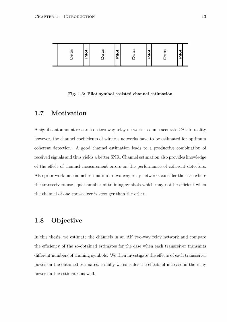
1.5 Pilot symbol assisted channel estimation . . . . . . . . . . . . . . . . . . 13
2.1 Cooperative network using a cellular set-up . . . . . . . . . . . . . . . . . 16
2.2 One-way relaying using a single relay . . . . . . . . . . . . . . . . . . . . 23
2.3 One-way relaying using multiple (N) relays . . . . . . . . . . . . . . . . . 24
2.4 Chain of transmitted frames . . . . . . . . . . . . . . . . . . . . . . . . . 25
2.5 One-way relay network with fixed relay . . . . . . . . . . . . . . . . . . . 27
2.6 Two-way relaying with reciprocal channels . . . . . . . . . . . . . . . . . 29
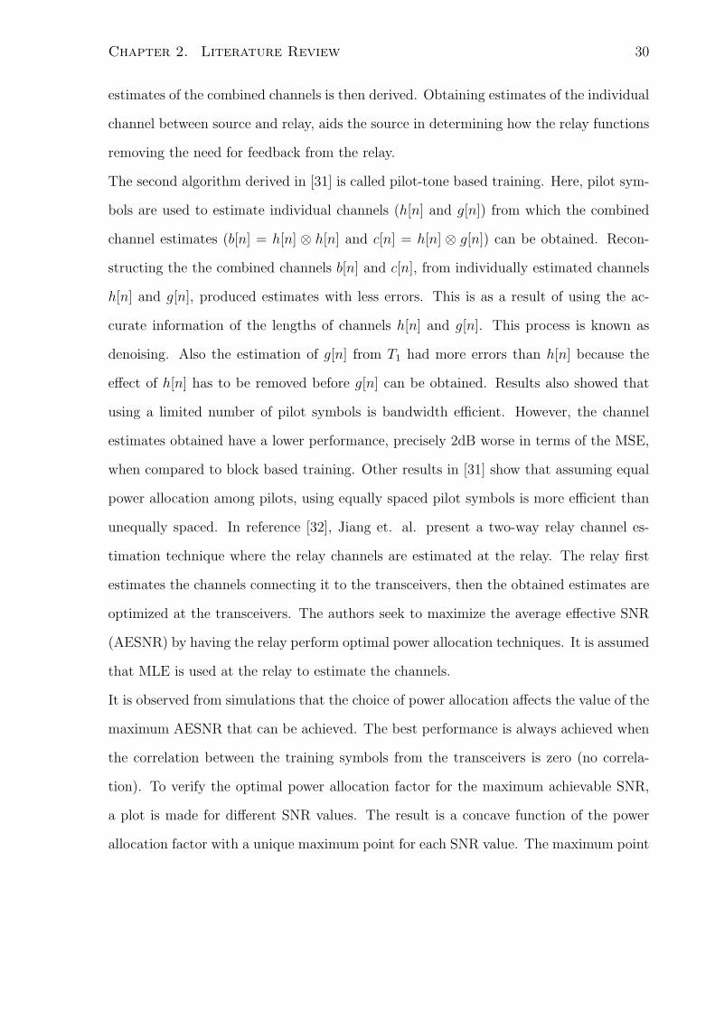
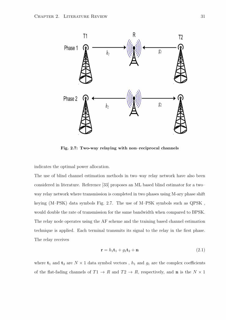
2.7 Two-way relaying with non–reciprocal channels . . . . . . . . . . . . . . 31
3.1 System Model . . . . . . . . . . . . . . . . . . . . . . . . . . . . . . . . . 35
4.1 MSE of hA versus P1 for varying training lengths of Nt1 and Nt2 = 5 . . 43
4.2 MSE of hA versus P1 for varying training lengths of Nt1 and Nt2 = 20 . . 44
4.3 MSE of hA versus P1 for varying training lengths of Nt2 and Nt1 = 20 . . 44
4.4 MSE of hB versus P2 for varying training lengths of Nt2 and Nt1 = 5 . . 45
4.5 MSE of hB versus P2 for varying Nt2 and Nt1 = 20 . . . . . . . . . . . . 46
4.6 MSE of hA versus P1 for varying Pr and Nt1 = 5 . . . . . . . . . . . . . . 47
ix
4.7 MSE of hA versus P1 for varying Pr and Nt1 = 20 . . . . . . . . . . . . . 47
4.8 MSE of hB versus P2 for varying relay power Pr and Nt2 = 5 . . . . . . . 48
4.9 MSE of hB versus P2 for varying relay power Pr and Nt2 = 20 . . . . . . 48
4.10 MSE versus Nt1 for total training length of 10 and P1 = P2 = 10 dBW . 49
4.11 MSE versus Nt1 for total training length of 10 and P1 = P2 = 20 dBW . 50
4.12 MSE versus Nt1 for total training length of 10 and P1 = P2 = 30 dBW . 50
4.13 MSE versus Nt1 for total training length of 20 and P1 = P2= 10 dBW . . 51
4.14 MSE versus Nt1 for total training length of 20 and P1 = P2 = 20 dBW . 51
4.15 MSE versus Nt1 for total training length of 20 and P1 = P2 = 20 dBW . 52
4.16 MSE versus Nt1 for total training length of 30 and P1 = P2 = 10 dBW . 53
4.17 MSE versus Nt1 for total training length of 30 and P1 = P2 = 20 dBW . 53
4.18 MSE versus Nt1 for total training length of 30 and P1 = P2 = 30 dBW . 54
4.19 MSE versus Nt1 for total training length of 40 and P1 = P2= 10 dBW . . 54
4.20 MSE versus Nt1 for total training length of 40 and P1 = P2 = 20 dBW . 55
4.21 MSE versus Nt1 for total training length of 40 and P1 = P2 = 30 dBW . 55
4.22 MSE versus Nt1 for total training length of 50 and P1 = P2 = 10 dBW . 56
4.23 MSE versus Nt1 for total training length of 50 and P1 = P2 = 20 dBW . 56
4.24 MSE versus Nt1 for total training length of 50 and P1 = P2 = 30 dBW . 57
4.25 MSE versus Nt1 for σ2hA
= 0.5 , σ2hB
= 1 and P1 = P2 = 10 dBW . . . . 58
4.26 MSE versus Nt1 for σ2hA
= 1, σ2hB
= 1 and P1 = P2 = 10 dBW . . . . . 58
4.27 MSE versus Nt1 for σ2hA
= 2 , σ2hB
= 1 and P1 = P2 = 10 dBW . . . . . 59
x

Nomenclature
(·)H denotes the Hermitian conjugate transpose of a matrix/vector
·T denotes transpose of matrix/vector
a boldface lowercase letters represent vectors
Re (·) denotes the real part of a complex matrix/argument
Im (·) denotes the imaginary part of a complex matrix/argument
j =√−1 denotes an imaginary unit
∥ · ∥ denotes norm of a matrix
| · | represents the amplitude of the complex number
∠z represents the phase of a complex number z
x represents the estimate of the element x
xi

Chapter 1
Introduction
1.1 Wireless Networks
The growth of wireless networks in the communications field has prompted a significant
amount of research. These networks provide advantages such as having mobile access to
a network, lower infrastructure setup costs, and the ability to support more users than a
wired network. However wireless channels are also prone to some problems.
Due to the high cost of bandwidth, wireless network designers need to find a way to
efficiently manage the bandwidth allocated to them. Wireless channels also have the
disadvantage of being susceptible to fluctuations of the quality of the transmission chan-
nels. Providing users the freedom to communicate while on the move presents some
difficulty in the design of wireless systems as the movement of users means the topology
of the network is constantly changing. These networks are also subject to interference
from different transmitting devices sending signals to a common receiver, from a single
transmitter sending signals to multiple receivers, or even between paired-up devices [1].
1
Chapter 1. Introduction 2
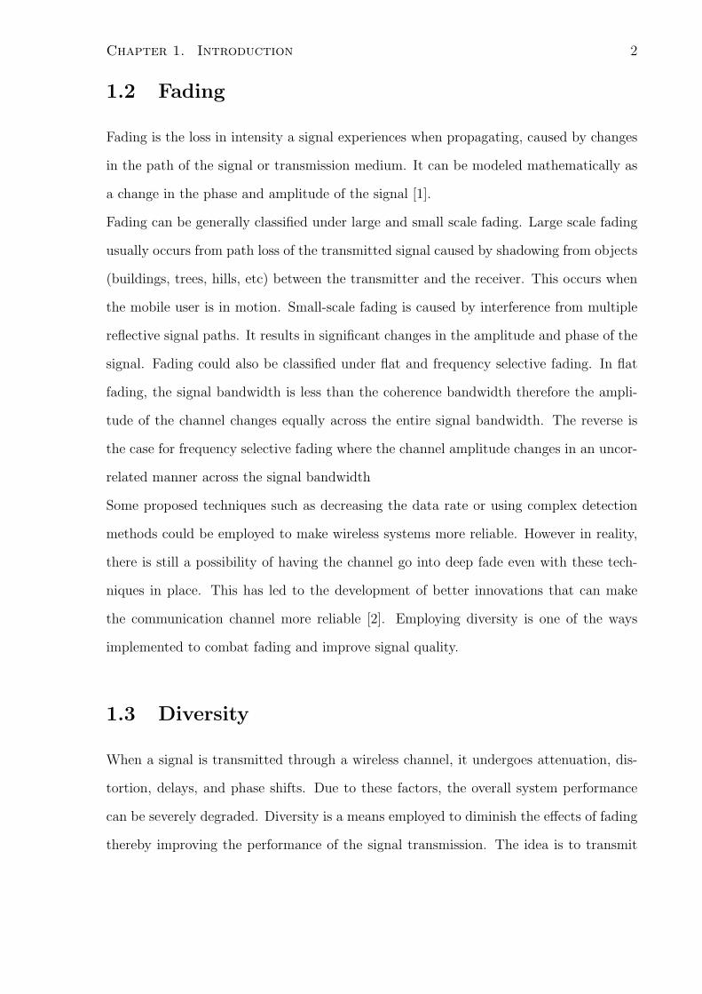
1.2 Fading
Fading is the loss in intensity a signal experiences when propagating, caused by changes
in the path of the signal or transmission medium. It can be modeled mathematically as
a change in the phase and amplitude of the signal [1].
Fading can be generally classified under large and small scale fading. Large scale fading
usually occurs from path loss of the transmitted signal caused by shadowing from objects
(buildings, trees, hills, etc) between the transmitter and the receiver. This occurs when
the mobile user is in motion. Small-scale fading is caused by interference from multiple
reflective signal paths. It results in significant changes in the amplitude and phase of the
signal. Fading could also be classified under flat and frequency selective fading. In flat
fading, the signal bandwidth is less than the coherence bandwidth therefore the ampli-
tude of the channel changes equally across the entire signal bandwidth. The reverse is
the case for frequency selective fading where the channel amplitude changes in an uncor-
related manner across the signal bandwidth
Some proposed techniques such as decreasing the data rate or using complex detection
methods could be employed to make wireless systems more reliable. However in reality,
there is still a possibility of having the channel go into deep fade even with these tech-
niques in place. This has led to the development of better innovations that can make
the communication channel more reliable [2]. Employing diversity is one of the ways
implemented to combat fading and improve signal quality.
1.3 Diversity
When a signal is transmitted through a wireless channel, it undergoes attenuation, dis-
tortion, delays, and phase shifts. Due to these factors, the overall system performance
can be severely degraded. Diversity is a means employed to diminish the effects of fading
thereby improving the performance of the signal transmission. The idea is to transmit
Chapter 1. Introduction 3
two or more copies of the signal through different channels with independent fading char-
acteristics, thereby reducing the probability of all channels being in deep fade at the same
time.
Different types of diversity techniques have been developed [3]. One of such techniques is
called frequency diversity. This is the use of multiple frequencies to transmit information.
In time diversity, the information is transmitted repeatedly in time at regular intervals
to ensure that temporally orthogonal channels exhibit statistically independent fading
characteristics.
As another form of diversity, polarization diversity modifies the electric and magnetic
fields of the signal carrying the information and uses them to send the same information.
In angle diversity, directional antennas are used to create independent copies of the trans-
mitted signal over multiple paths.
In spatial diversity, multiple transmit antenna (transmit diversity) or multiple receive
antenna (receive diversity) are used to transmit and/or receive signals providing multi-
ple independent paths. Such spatial diversity schemes improve the network performance
using available power resources and bandwidth [4].
1.3.1 Spatial Diversity
The need for diversity techniques in wireless networks is emphasized by fading. The
multiple-input multiple-output (MIMO) system is a smart antenna technology using
multiple transmit and receive antennas for communication to provide spatial diversity.
MIMO systems are capable of increasing area coverage and often achieve higher signal-
to-noise ratios (SNRs) . They can also increase the channel data rate. These advantages
have made MIMO systems very attractive in wireless communications.
The use of MIMO systems require techniques to efficiently transmit and combine the
multiple copies of the signal. These are called transmit and receiver diversity techniques.
Transmit diversity implies sending multiple copies of a signal through different antennas.

Chapter 1. Introduction 4
It is useful in systems with more signal processing and power availability at the transmit
end of the communication network. Knowledge of the channel is important in the design
of transmit diversity.
Receive diversity combines the independent signals resulting from the use of multiple
receive antennaes. The output of the combiner is then passed though a demodulator.
Different receiver diversity techniques have been proposed [5]. One of such is known
as selection combining. Here only the antenna with the highest SNR is offered to the
receiver after a selection process. All antennas must have established connections for
their SNRs to be measured. Outage probability decreases as the number of antennas
is increased however this is not a linear increment. The power gain diminishes as the
number of antennas become large.
Threshold combining outputs the first signal whose SNR is above a given threshold. It
stays on that signal until it drops below the threshold and then it switches to another
antenna. It is easier to implement than the selection combining technique because it does
not require the need for a sole receiver for each antenna output .
Maximal ratio combining (MRC) outputs the weighted sum of all antenna signals. Phase
adjustment is required to correctly combine the signals for maximum SNR. Unlike selec-
tion combining, power gain increases linearly with increase in the number of antennas.
Equal gain combining applies the same weight to signals on each antenna and then com-
bines them. It has a better performance than selection combining since all available paths
are used.
Beamforming is a spatial diversity technique which strengthens the signal of interest and
attenuates the signals from other directions. This is achieved by adjusting the amplitude
and phase of the desired signal.

Chapter 1. Introduction 5
1.4 User Cooperation Diversity
Cooperative communication is a means for single-antenna users to share their resources
so that they can get some of the advantages MIMO systems. Partnered users help each
other send their information by providing multiple paths to the receiver resulting in what
is known as a relay network [6] and [7]. Since the paths are statistically independent,
cooperation results in spatial diversity. The source and the relayed signals are combined
at the receiver for detection.
Cooperation could lead to an increase in communication costs. There might be need
for more hardware so that information can be shared between sources. Also, the use of
relays may lead to increase in amount of power required. Notwithstanding these costs,
there is a considerable improvement specifically in bandwidth efficiency, communication
speed, prolonged battery lifetime, and an increase in the area of coverage.
1.5 Relay Networks
When a transmitter and a receiver are unable to communicate with each other because
of the distance between them or fading of the channel, they can be connected by one
or multiple relay nodes to create an alternate route, creating a relay network. Relaying
increases the distance which transmitted signals travel and could resulting in extending
the battery life of the transmitter and reduced signal interference.
The authors of [8] have presented the general idea and some of the schemes behind co-
operative communication. The authors discuss some schemes the relay applies to the
signal it receives before retransmitting. One of such schemes is decode–and–forward
(DF) approach, where the user aims to decode the signal received from its partner before
forwarding it to the receiver. The receiver has to know the characteristics of the relay
channel for best detection. This method adjusts to channel conditions, and if the trans-
mitted signals are not correctly decoded, cooperation can make signal detection at the

Chapter 1. Introduction 6
receiver difficult.
A second strategy is the compress–and–forward (CF) method, where users quantize and
compress their partner’s information and then send that to the receiver. At the receiver,
the transmitted signal is decoded to obtain the original signal.
Another relaying scheme is the amplify–and–forward (AF) method where each user am-
plifies the signal received from its partner before retransmitting to the receiver. Because
of its ease of implementation, this method has been widely used in analyzing cooperative
communication systems.
Relaying can be done in one direction, i.e., one-way relaying, where one or more trans-
mitters, transmits information through a relay or multiple relays to the receiver. This
communication is usually carried out in two time-slots. In the first time-slot, the trans-
mitter sends its signals to the relay which is then processed using a relaying scheme. A
modified signal is produced and sent to the receiver in the second time-slot.
When two transceivers exchange data through one or multiple relay nodes, the network
created is referred to as a two-way relay network. It is a cooperation method proposed
to reduce the spectral efficiency loss that arises in half-duplex one–way relay systems.
1.5.1 Two-Way Relay Networks
Two-way communication channel was first introduced in [9], for point-to-point communi-
cation. The use of relays for two-way communication is known as bi-directional relaying
or two-way relaying. Here two transceivers exchange information through one or more
relay nodes. In doing so, the spectral efficiency loss obtainable in one-way relay networks
is combatted.
In [10], relaying techniques used for two-way relaying are described. The first is called
the traditional technique. It uses four time-slots to complete the transmission and re-
ception of signals between two transceivers (see Fig. 1.1). Each transceiver sends their
information to the relay one at a time using one time-slot each. The relay then sends the

Chapter 1. Introduction 7
received processed information to both transceivers using two time-slots as well. As the
Fig. 1.1: Two-way relay phases using four time-slots
exchange of information requires four time-slots, it is not bandwidth efficient.
Another method discussed in [10] uses three time-slots as shown in Fig. 1.2. Both
transceivers transmit their signals to the relay one at a time in the first two time-slots
and during the third time-slot, the relay forwards the exclusive OR (XOR) of the decoded
signal to both transceivers. The transceivers obtain the signal they want by executing an
XOR on its transmitted symbol and its received signal. As an alternative, the received
signal at relay could be demodulated and decoded to obtain the transmitted data. This
data is then re-encoded and re-modulated before retransmitting to the transceivers. This
process is known as digital network coding [11].
A third method presented in [10] is the two time-slot scheme, where both transceivers
send their information to the relay in the first time-slot at the same time and then the
relay retransmits the processed signal in the second time-slot Fig. 1.3. Using two time-
slots for data exchange by two transceivers improves the spectral efficiency incurred in
one-way relay networks. The initiative behind two-way relaying is that, to decode the

Chapter 1. Introduction 8
Fig. 1.2: Two-way relay phases using three time-slots
Fig. 1.3: Two-way relay phases using two time-slots
data from the other transceiver, each transceiver has to cancel the interference of its own
signal from the signal it receives.
1.6 Channel Estimation
Channel estimation is the process of describing the effects of a channel model on a given
input signal so that the signal can be coherently detected. To obtain a good estimator,

Chapter 1. Introduction 9
first the data has to be modeled mathematically. A channel model is a mathematical
representation of the amplitude and phase of the transfer function of a channel.
Fig. 1.4 depicts a block diagram of the basic channel estimation process. It can be de-
duced that , a good estimator is one that is successful in producing the smallest mean
squared error (MSE) with an algorithm that is not too computationally intense. Channel
Fig. 1.4: Basic channel estimation process
estimation is one of the most essential technologies required for wireless networks. Knowl-
edge of the channel state information (CSI) not only makes it easier for signal detection,
but it is also useful in the allocation of power and design of capacity achieving systems.
To make a good recovery of the transmitted signal, the effect of the channel on it can
be estimated. An estimator is used to deduce an unknown value from measured data.
Without properly estimating the channels, the benefits offered by cooperative systems
could be lost. A good channel estimate leads to a productive combination of received
Chapter 1. Introduction 10
signals and thus yields a better SNR. When compared to non-coherent detection, co-
herent detection is more power efficient, thereby prompting a lot of research on channel
estimation.
1.6.1 Types of Estimators
Estimators are signal processing methods used to extract information from noisy obser-
vations. The unknown parameters of the information are estimated from some measured
data with a random component. Different types of estimators exist that could be applied
to estimate wireless channels. The minimum variance unbiased estimator (MVUE) is
an efficient estimator. For all possible values of the parameter to be estimated, it has
the smallest variance among other unbiased estimators. However, even if this estimator
exists, it may not be possible to find it. Some approaches have been proposed to help
determine the MVUE. One such approach is to determine the Cramer-Roa lower bound
(CRLB) [12]. The CRLB provides a point of reference for any unbiased estimator. It
puts a lower bound on their variances. Therefore if there exists an estimator that attains
the CRLB, then that estimator is the MVUE.
Best linear unbiased estimators (BLUE) [12] is suitable in practice because it can be
used in situations where the total knowledge of the probability density function (pdf) is
not available. It is a suboptimal estimator but its use is validated if its variance can be
determined and if it meets the requirements of the problem to be solved. If there exists
a linear data of the form
x = Hθ + w (1.1)
where H is a known matrix, θ is a vector of the parameters to be estimated, and w is a
noise vector with zero mean and covariance C, then BLUE can be expressed mathemat-
ically as
θ = (HTC−1H)−1HTC−1x (1.2)
Chapter 1. Introduction 11
The minimum mean square error (MMSE) estimator is a bayesian estimator which, as
the name implies, minimizes the mean square error of the estimates of a random variable
using some prior knowledge of the variable such as its pdf. Sometimes it may not be
possible to determine the MMSE estimator in a closed form. The linear minimum mean
square error (LMMSE) estimator can then be used because it attains minimum mean
square error among all estimators of linear form or else it will be suboptimal. They are
simpler than optimal bayesian estimators while maintaining the MMSE criterion.
The maximum a posteriori (MAP) estimator is another bayesian estimator which maxi-
mizes the posterior distribution of a random variable.
θ = argmaxθ
p(θ|x) (1.3)
It can use an observed data to determine the point estimate of an unknown variable [12].
The least square error (LSE) estimator minimizes the squared difference between a given
signal s[n] and an observed signal x[n]. Minimum difference is determined by the LS
error criterion
J(θ) =N−1∑n=0
(x[n]− s[n])2 (1.4)
where the interval of observation is n = 0, 1, ..., N − 1. Therefore the LSE is the value
of θ that minimizes J(θ) [12]. LSE cannot be said to be optimal and no probabilistic
assumptions can be made about the data . It is however easy to implement since it does
not require the use of any data statistics.
The maximum likelihood estimator(MLE) is used to find the parameter value that makes
the observed data most likely [13]. It is frequently used for large data records. The pdf of
the data model should be known. MLEs are widely used because of its ability to produce
an efficient estimator with minimum variance if such an estimator exists. It is also the
most applied approach to obtaining practical estimators [12].

Chapter 1. Introduction 12
1.6.2 The Maximum Likelihood Estimator
MLEs aim to estimate the value of an unknown parameter which maximizes the proba-
bility that a given measurement is observed. Given that g is a function whose conditional
pdf is described by;
f(g|ζ) (1.5)
where ζ is the parameter that needs to be estimated, the MLE is defined by
ζ = argmaxζ
f(g|ζ). (1.6)
1.6.3 Channel Estimation Methods
There are basically three types of channel estimation methods. The training sequence,
semi-blind and the blind channel estimation methods.
Blind channel estimation methods do not use training symbols. Training is carried out
while information is being transmitted. It is a bandwidth efficient technique albeit com-
plex to compute and difficult to implement [14].
In the semi-blind channel estimation, a part of the input vector is known. It makes
use of the fact that there are known symbols inserted in most data packets. Therefore
depending on whether or not the observation of the known or unknown data is used, it
switches between training-based and blind estimations [14].
In training based methods, training symbols are used to provide a priori knowledge to
the receiver. These symbols are inserted in the data frame and transmitted through the
channel (see Fig. 1.5). These training symbols are then used to estimate the channel
coefficients. Training based estimators are very efficient when the channel variation is
slow. This method is easier to implement, it is not computationally complex and it pro-
duces accurate estimates quickly, leading to its popular use. The type of method chosen
results in a compromise between efficient bandwidth usage and complexity of the channel
estimator [14].
Chapter 1. Introduction 13
Fig. 1.5: Pilot symbol assisted channel estimation
1.7 Motivation
A significant amount research on two-way relay networks assume accurate CSI. In reality
however, the channel coefficients of wireless networks have to be estimated for optimum
coherent detection. A good channel estimation leads to a productive combination of
received signals and thus yields a better SNR. Channel estimation also provides knowledge
of the effect of channel measurement errors on the performance of coherent detectors.
Also prior work on channel estimation in two-way relay networks consider the case where
the transceivers use equal number of training symbols which may not be efficient when
the channel of one transceiver is stronger than the other.
1.8 Objective
In this thesis, we estimate the channels in an AF two-way relay network and compare
the efficiency of the so-obtained estimates for the case when each transceiver transmits
different numbers of training symbols. We then investigate the effects of each transceiver
power on the obtained estimates. Finally we consider the effects of increase in the relay
power on the estimates as well.

Chapter 1. Introduction 14
1.9 Methodology
We utilize the MLE for our channel estimation process. The MLE has the advantage
of being a flexible estimator making it applicable to a various data and models. The
performance of the obtained estimates are then evaluated based on their MSE.
1.10 Thesis Organization
The rest of this thesis is organized as follows. The next Chapter describes various MIMO
and cooperative communication techniques and channel estimation methods. We analyze
and compare these methods with our own method. In Chapter 3, we derive the MLE.
We describe the system model used in this thesis and then the problem formulation. We
then solve the channel estimation problem for different number of training symbols at
both transceivers. We present our simulation results and discuss the effects of transmit
power on the obtained estimates in Chapter 4. Chapter 5 concludes the thesis.
Chapter 2
Literature Review
In this Section, different applications of relay networks is discussed. We describe system
models and approaches resembling ours that maximize system throughput and efficiency.
We then analyze various techniques proposed in literature on channel estimation in relay
networks.
2.1 Cooperative Communication
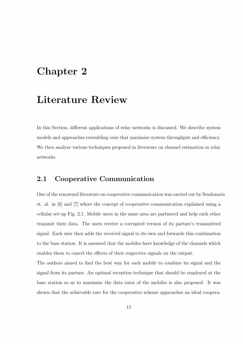
One of the renowned literature on cooperative communication was carried out by Sendonaris
et. al. in [6] and [7] where the concept of cooperative communication explained using a
cellular set-up Fig. 2.1. Mobile users in the same area are partnered and help each other
transmit their data. The users receive a corrupted version of its partner’s transmitted
signal. Each user then adds the received signal to its own and forwards this combination
to the base station. It is assumed that the mobiles have knowledge of the channels which
enables them to cancel the effects of their respective signals on the output.
The authors aimed to find the best way for each mobile to combine its signal and the
signal from its partner. An optimal reception technique that should be employed at the
base station so as to maximize the data rates of the mobiles is also proposed. It was
shown that the achievable rate for the cooperative scheme approaches an ideal coopera-
15

Chapter 2. Literature Review 16
Fig. 2.1: Cooperative network using a cellular set-up
tion where the channel is noiseless. Also a better channel between the users leads to a
better achievable rate, which means less power consumption.
The authors also showed that cooperation reduces the probability of outage more than
is observed in non-cooperative systems. This implies that cooperative systems are more
like to be robust in systems with large channel variations. Also observed is that cooper-
ation leads to increases in the capacity of the system as cellular coverage area increases.
A disadvantage of cooperative networks could be the increased complexity in the design
of the receivers. For security reasons, user data may have to be encrypted so that their
partners can transmit their signals without detecting them.
Reference [7] describes the code division multiple access (CDMA) implementation and
performance of the concepts described in [6]. CDMA uses spread spectrum coding tech-
niques to give multiple users access to a given channel. An advantage of applying the
Chapter 2. Literature Review 17
CDMA technology is the ability to accommodate as many users as possible as long a
reasonable quality of service can be maintained. The authors showed that using CDMA
results in a higher data transmission rate and that the transmitted signals are also less
sensitive to variations in the channel. As a result of increase in the data rate, less power
is required for users leading to an increase in the battery life of the mobiles thereby
lengthening the life of the network. Obtained results also showed that even when the
CSI is not known, cooperative networks have larger achievable rates than non-cooperative
networks.
2.2 Relaying Protocols and Applications
Since the work of Sendonaris et. al. in [6] and [7], a flurry of research has been carried
out on applying the relaying schemes described in Chapter 1 to cooperative networks.
In the following sections , we provide existing literature that describes the application
of the these relaying schemes to one–way and two–way relay networks. We also examine
different techniques applied to improve the performance of these relay networks. These
techniques include power allocation, relay selection and beamforming.
2.2.1 One–Way Relaying
A relay network could be set up with a single or multiple relay nodes. In the case of mul-
tiple relay node networks, the concept of relay selection may be needed. Relay selection
is a cooperative communication scheme that seeks to use the relay path that will provide
the best quality of service without using too much resources. If efficiently implemented,
it could achieve full diversity. In reference [15], the AF and DF schemes are applied to a
one–way relay network with multiple relays. The AF and DF schemes are combined with
novel techniques called selection relaying and incremental relaying. Assuming knowledge
of the CSI, selection relaying operates by having the users participating in cooperation,

Chapter 2. Literature Review 18
carry out channel measurements so as to determine the reliability of the channels be-
tween them. The information obtained from these measurements are then used to select
the best communication relay path. Incremental relaying uses feedback in the form of a
single bit provided by the destination, to detect the success or failure of the direct link
between the source and the destination. The relay only participates in the data trans-
mission process if the destination provides a negative feedback such as if the transmitted
bits are not decoded correctly. As SNR is increased, a decrease in outage probability is
observed for the proposed methods when compared to the sole implementation of the AF
and DF schemes.
In [16], the authors propose a distributed cooperative protocol for selecting the most
appropriate relay to use for information transmission in a one-way relay network with
multiple relay nodes. Without requirement of knowledge of the network topology, the
relay nodes observe the instantaneous conditions of the channel between the source and
the destination in a slow fading environment and these relay nodes decide which channel
is strongest for use in signal transmission. Explicit communication among the relays is
also not required and successful selection of a relay depends on the channel statistics at
that time. The source and relay transmit their signals in orthogonal time–slots. This
was shown to provide diversity gains in the order of the number of relays in the network.
In a cooperative network with multiple relay nodes, the available power and channel
resources may be equally distributed among the relays. All the relays could then be
made to participate in the signal transmission process. This technique is evidently sub-
optimal.
Reference [17] has proposed a power distribution scheme where power is allocated to
each relay node based on CSI and channel statistics. The scheme for choosing the best
node for relaying information using the complete CSI is then proposed . This approach
is different from that proposed in [16] in that the selection algorithm is carried out at
the destination. It is assumed that the destination has knowledge of all channel gains.
Chapter 2. Literature Review 19
The scheme is less complex because the destination only makes the required relay node
selection and notifies the selected node. The scheme was shown to have a lower outage
probability and higher throughput as it only has to repeat its information once than
when all nodes take part in the relay selection and communication process.
The authors of [18] analyze different power allocation strategies and CSI assumptions
for the optimum one–way relay network. The network considered is a three-node relay
network made up of a source, relay and destination. The signal received at the desti-
nation is composed of the signal transmitted directly to the destination and the signal
transmitted to the destination through the relay (relayed signal). The objective of this
work is to determine the best power allocation at the source and the relay to maximize
the quality of service at the receiver. First, the case with full and partial CSI at the
source, relay and destination is considered. It was observed that using the DF scheme
and with no connection between the source and the destination, power allocation at the
source and relay should be equal for optimal quality of service. If there is a connection
between the source and destination, then more power should be allocated to the source
as it will be transmitting both to the relay and directly to the destination. It was also
concluded that the choice of allocating power should only be considered when source-
relay and relay-destination channels are decent compared to the source-destination link.
If not, all power should be allocated to the source. Compared to the DF scheme, the AF
scheme showed a better outage probability when the SNR is high.
2.2.2 Two–Way Relaying
Communication between two terminals can be done in either half-duplex or full-duplex
mode. In full-duplex mode, the communicating terminals are able to send their respec-
tive data to each other at the same time. Half-duplex systems incur spectral efficiency
loss because of the inability to transmit data in two directions at the same time.
Reference [19] discusses a method called two-path relaying that makes up for this spec-
Chapter 2. Literature Review 20
tral efficiency loss in a cooperative network. The network model is composed of two
transceivers and two relays. Assuming there is no direct connection between both
transceivers, the first relay receives data from the first transceiver during odd numbered
time-slots (i.e. 1, 3, 5, ...) and forwards the data after either amplifying or decoding
to the end transceiver during even numbered time-slots (i.e. 2, 4, 6, ...). The reverse is
the case for the second relay except during the very first time-slot when it is silent. The
loss encountered in conventional half-duplex transmissions is avoided as the transceiver
is transmitting a new data set at every time-slot.
Reference [20] describes a way to optimally allocate power to relay nodes in a pairwise
communication network. The relays help paired up transceivers exchange information.
It is assumed the channel between each pair of transceivers is orthogonal. Relaying
schemes applied to this model are the AF, CF, decode–and-XOR–forward (DXF) and
decode-and-superposition-forward (DSF) schemes. With the DXF scheme, the relay de-
codes the received information then retransmits the XORed version of the signal to the
destination and with the DSF scheme, the relay re-encodes its received signals individu-
ally before it retransmits to the destination.
The performances of these relaying schemes are examined for a two-phase and three-phase
relaying techniques explained in [10]. Because of the use of direct links, the three-phase
technique gives a better performance than two–phase when the power at each relay is low
but as power increases, the two-phase protocol performs better. As it is more efficient to
forward XORed signals than individual ones, the sum rate of the DXF relaying scheme
is better than that of DSF until the upper bounds are reached. It was also observed that
the CF scheme always performs better than the AF scheme. Reference [20] shows that
with a given power budget at the relay, an efficient relaying scheme can be chosen so as
to maximize the sum rate in a given communication network.
Reference [21] considers a two-way relay network with multiple relays where the relay
which provides the best CSI connection during each transmission session is selected. The

Chapter 2. Literature Review 21
best relay is determined by assigning a weight gain for each relay path based on the
sum rate of the relay that maximizes the network channels. This proposed scheme is
called two-way relaying with opportunistic selection (TWR-OS). Numerical simulations
obtained show a reduction in sum-rate loss in half–duplex relaying. Also increase in the
number of relay nodes yield an increase in the diversity order. The performance bounds
derived for TWR-OS compared favorably with the simulations.
Another spatial diversity technique that can applied to improve the quality of signal
propagating through a network is beamforming. In [10], the authors derive a way to
calculate the optimal beamforming weight and transceiver transmit power in a two–way
relay network applying the two time-slots relaying technique. They considered two meth-
ods to compute the optimal beamforming weight vector and transceiver transmit power
subject to the receive quality of service being above a given threshold. One way was
to minimize the total network transmit power where they found a unique solution using
this method. Thus an iterative algorithm can be used to obtain the optimal beamform-
ing weight vector. Another way considered in [10] is the SNR balancing method where
the smallest SNR of the two transceivers is maximized while keeping the total transmit
power lower than a given threshold. The authors showed that this solution is also unique
and can be obtained using iterations. Also increase in network size does not affect the
amount of bandwidth needed to obtain the beamforming weights.
Reference [22] describes a general rank approach to beamforming using a single antenna
transmitter, a single-antenna receiver, and a multi-antenna relay node. The transmit-
ter sends a signal vector to the relay which multiples it by a general-rank beamforming
matrix and retransmits the signal to the receiver using other free antennas. In [22], it
is shown that by maximizing the SNR at the receiver subject to a constrained transmit
power at the relays, gives a closed-form solution for the beamforming matrix.
The references on relay networks from [6] - [22], have all assumed that the CSI is known
which may not be applicable. Therefore channel estimation techniques could be incor-

Chapter 2. Literature Review 22
porated in the above research to obtain more realistic performances.
2.3 Channel Estimation in One–Way Relay Networks
As mentioned earlier, channel estimation is an essential process in coherent signal detec-
tion. In this Section, we review previous works on relay schemes and channel estimation
in one-way relay networks most of which apply the AF relay scheme.
Literature on the estimation of channels in relay networks present schemes used to ei-
ther estimate the cascaded or disintegrated channels. The cascaded channels are made
up of the joint links comprising the source-relay and the relay-destination channels
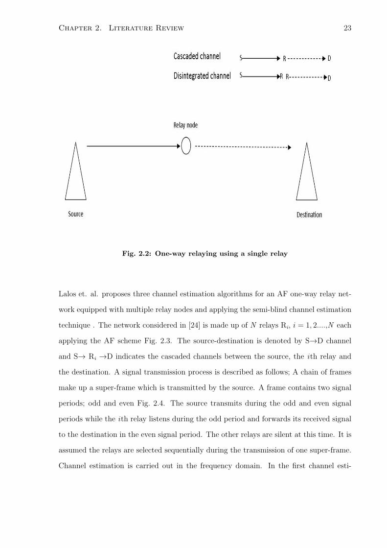
(Fig. 2.2).The disintegrated channel is the separated source-relay and relay-destination
channels.
In [23], two channel estimation methods comparing estimates of the cascaded and dis-
integrated channels are presented. The first method performs channel estimation at the
receiver for the cascaded channels. In the second method, the disintegrated source-relay
channel is estimated at the relay while the relay-destination channel is estimated at the
receiver. Using the disintegrated method of channel estimation involves sending a quan-
tized version of the obtained source-relay channel estimates to the destination.
The MSE performance of the cascaded and disintegrated channel estimates is evaluated
using different numbers of pilots for three relay-location cases where the relay is close
to the source, the relay is close to the destination, and the relay is at an equal distance
between the source and destination. When the relay is close to the source, it is observed
that cascaded channel estimation performs slightly better than disintegrated channel es-
timation when the number of pilots is high. The performance is however, the same for
the disintegrated and cascaded channel estimators when the number of pilots is low. Ir-
respective of the number of pilot symbols used, placing the relay close to the destination
or at an equal distance gave the same performance.
Chapter 2. Literature Review 23
Fig. 2.2: One-way relaying using a single relay
Lalos et. al. proposes three channel estimation algorithms for an AF one-way relay net-
work equipped with multiple relay nodes and applying the semi-blind channel estimation
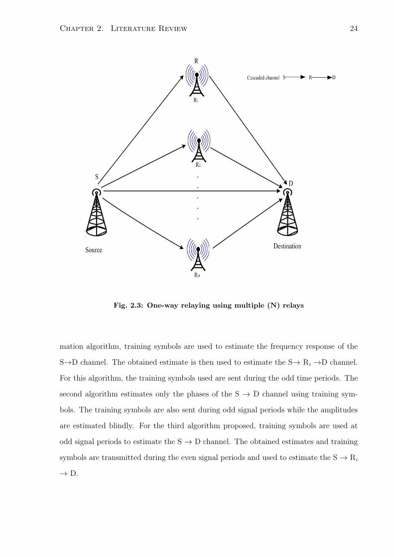
technique . The network considered in [24] is made up of N relays Ri, i = 1, 2....,N each
applying the AF scheme Fig. 2.3. The source-destination is denoted by S→D channel
and S→ Ri →D indicates the cascaded channels between the source, the ith relay and
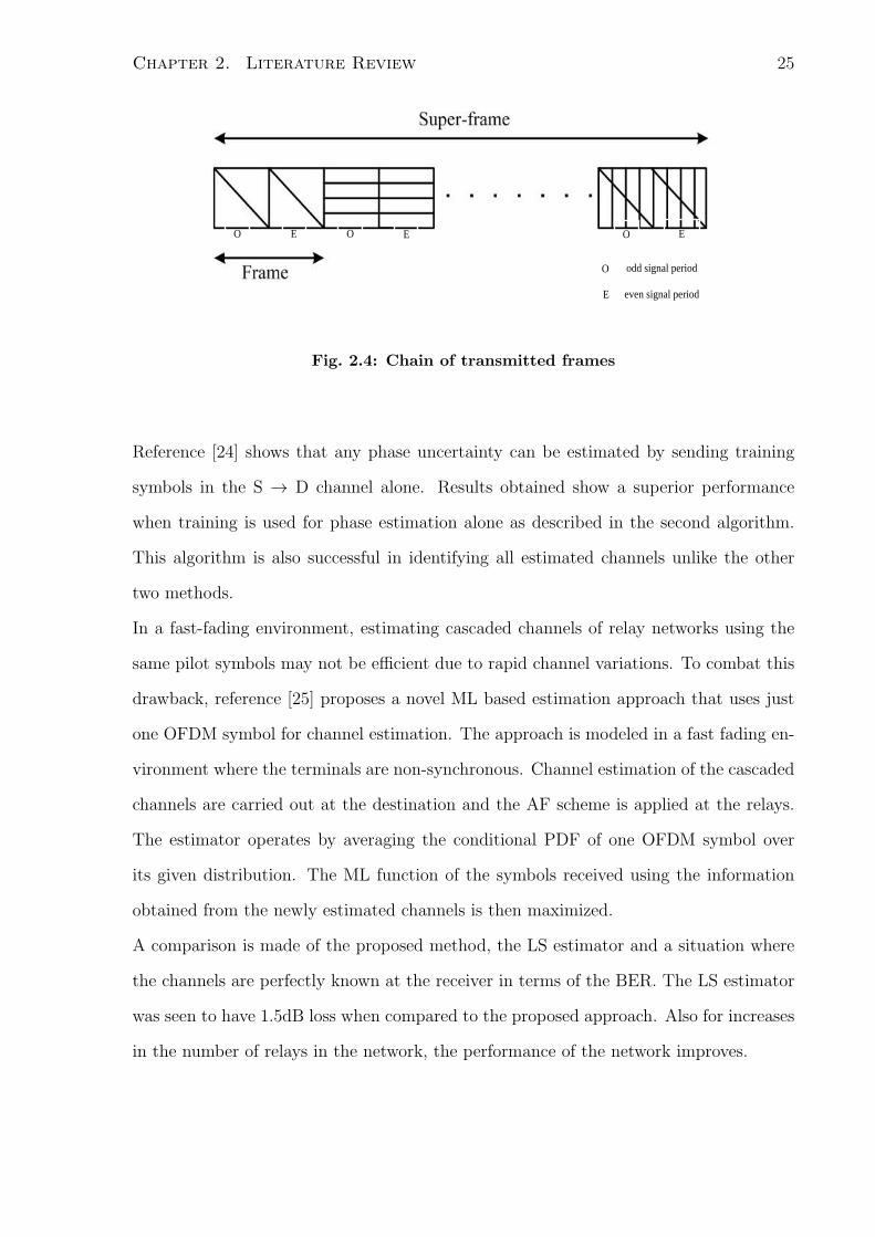
the destination. A signal transmission process is described as follows; A chain of frames
make up a super-frame which is transmitted by the source. A frame contains two signal
periods; odd and even Fig. 2.4. The source transmits during the odd and even signal
periods while the ith relay listens during the odd period and forwards its received signal
to the destination in the even signal period. The other relays are silent at this time. It is
assumed the relays are selected sequentially during the transmission of one super-frame.
Channel estimation is carried out in the frequency domain. In the first channel esti-
Chapter 2. Literature Review 24
Fig. 2.3: One-way relaying using multiple (N) relays
mation algorithm, training symbols are used to estimate the frequency response of the
S→D channel. The obtained estimate is then used to estimate the S→ Ri →D channel.
For this algorithm, the training symbols used are sent during the odd time periods. The
second algorithm estimates only the phases of the S → D channel using training sym-
bols. The training symbols are also sent during odd signal periods while the amplitudes
are estimated blindly. For the third algorithm proposed, training symbols are used at
odd signal periods to estimate the S → D channel. The obtained estimates and training
symbols are transmitted during the even signal periods and used to estimate the S→ Ri
→ D.
Chapter 2. Literature Review 25
odd signal period
even signal period
O E EO O E
O
E
Fig. 2.4: Chain of transmitted frames
Reference [24] shows that any phase uncertainty can be estimated by sending training
symbols in the S → D channel alone. Results obtained show a superior performance
when training is used for phase estimation alone as described in the second algorithm.
This algorithm is also successful in identifying all estimated channels unlike the other
two methods.
In a fast-fading environment, estimating cascaded channels of relay networks using the
same pilot symbols may not be efficient due to rapid channel variations. To combat this
drawback, reference [25] proposes a novel ML based estimation approach that uses just
one OFDM symbol for channel estimation. The approach is modeled in a fast fading en-
vironment where the terminals are non-synchronous. Channel estimation of the cascaded
channels are carried out at the destination and the AF scheme is applied at the relays.
The estimator operates by averaging the conditional PDF of one OFDM symbol over
its given distribution. The ML function of the symbols received using the information
obtained from the newly estimated channels is then maximized.
A comparison is made of the proposed method, the LS estimator and a situation where
the channels are perfectly known at the receiver in terms of the BER. The LS estimator
was seen to have 1.5dB loss when compared to the proposed approach. Also for increases
in the number of relays in the network, the performance of the network improves.

Chapter 2. Literature Review 26
Implementing training based channel estimation techniques requires the use of some of
the bandwidth available. This means less bandwidth would be available for data trans-
mission. In reference [26], a means of channel estimation is designed that reduces the
estimation overhead required for obtaining CSI while making use of the minimum amount
of training possible. Using the network described in Fig. 2.5, this proposed method ex-
ploits the fact that the channel between the base station and the relay station (hsr) is
fairly stable because these nodes are fixed. Because of this stability, it is not constantly
required to estimate the hsr channel. The hrs channel is then constant over the time used
to estimate the source–destination channel (hsd) and the relay–destination (hrd) chan-
nels. Therefore when the base station is trying to estimate hsd and hrd, hsr is already
known. Using this pre-knowledge, the channel estimation overhead is thereby reduced.
A pilot signal is sent by the mobile station, amplified at the relay and forwarded to the
base station providing the base station with the CSI between the mobile station and the
relay station.
When using training symbols in channel estimation, it is important to determine the
optimum number of training symbols to use the minimum amount of bandwidth while
producing efficient channel estimates in the training phase.
Reference [27] describes a channel estimation technique based on LMMSE for a relay
network employing the AF relaying scheme. The system model consists of a source and
destination node equipped with a single antenna and multiple single-antenna relays. It
is assumed that the channels between the source and the relays (backward channel) and
that between the relays and destination (forward channel) are constant for a given period
of time during which it estimated.
The authors of [27] considered three cases to evaluate the performance of their proposed
channel estimation method. In the first case, the relays use training symbols to estimate
the forward and backward channels. The destination begins transmission by sending
training symbols to the relays which the relays use to estimate the forward channel. Once

Chapter 2. Literature Review 27
Fig. 2.5: One-way relay network with fixed relay
the forward channel is estimated, the source begins to send training symbols through the
relays to the destination. The backward channel is estimated using the training symbols
sent to the destination. In the second case, the relays have complete knowledge of the
channel hence there is no need to send training symbols from the destination. The relays
amplify the received symbols obtained from the source and sends it to the destination.
For the third case, the relays have no knowledge of the channels. As in the second case
the relay amplifies and forwards symbols obtained from the source.
Results obtained in [27] show that an increase in the number of relays lead to an increase
in the mean square error. Except at low SNRs, all three cases yield the same gain. The
state of perfect channel knowledge yields a better gain at this region. More results ob-
tained show that if the period during which the training symbols are sent is small, the
relays do not make a good estimate of the channels. Thus the capacity is lower than for
Chapter 2. Literature Review 28
a larger symbol period.
2.4 Channel Estimation in Two–Way Relay Networks
A significant amount of work on channel estimation in one–way relay networks have been
done [23]– [28]. However as two-way relay networks garner interest, it has become neces-
sary to study methods and efficient protocols to estimate the channels in such network.
Channel estimation in two-way relay networks is more complex as the estimates are not
only required for coherent signal detection, but also for self-interference cancelation at
the transceivers.
In [29], self-interference suppression techniques rather than pilot sequences are used in
the estimation of the channels in a two–way relay network employing the DF scheme and
using two time–slots. Self–interference contains data known by a transceiver thus its ef-
fects can be canceled out before the data is decoded. First, estimates of the channels are
obtained using the LMMSE estimator in the second phase of the transmission process.
Then the accuracy of these obtained estimates are improved using a decision-directed
iterative process which jointly estimates the channel and performs data detection. Sim-
ulation results show that the proposed method has a lower MSE at low SNRs than a
system where only pilot symbols are used. However, the pilot assisted estimators gave a
better performance at higher SNRs.
For a two–way relay network applying the AF scheme, reference [30] also applies self-
interference suppression in channel estimation. A lower bound on the training based
individual and sum-rate of the transceivers is determined. Due to errors observed during
channel estimation, it is not possible to obtain perfect signal interference cancelation
therefore residual self-interference affects the sum-rate. A search for the optimal power
allocation among the transceiver and relay nodes to maximize these so-obtained lower
bound is derived. Also an optimal power allocation between training and data transmis-

Chapter 2. Literature Review 29
h[n] g[n]
h[n] g[n]
Fig. 2.6: Two-way relaying with reciprocal channels
sion that also maximizes the lower bounds is determined.
2.4.1 ML–Based Channel Estimation
Feifei et. al. consider the ML channel estimation of a half duplex two-way relay net-
work which uses the AF relaying scheme and orthogonal frequency division multiplexing
(OFDM) modulation [31]. The network consists of two transceivers which share their in-
formation through a relay with reciprocal channels Fig. 2.6. OFDM spreads information
over many frequency spaced orthogonal carriers. Two training algorithms are proposed
in [31].
The first is called block based training where a whole OFDM block is used to estimate
the combined T1 → R → T2 channels (b[n] = h[n] ⊗ h[n] and c[n] = h[n] ⊗ g[n], where
⊗ means circular convolution). An algorithm that obtains individual channels from the
Chapter 2. Literature Review 30
estimates of the combined channels is then derived. Obtaining estimates of the individual
channel between source and relay, aids the source in determining how the relay functions
removing the need for feedback from the relay.
The second algorithm derived in [31] is called pilot-tone based training. Here, pilot sym-
bols are used to estimate individual channels (h[n] and g[n]) from which the combined
channel estimates (b[n] = h[n] ⊗ h[n] and c[n] = h[n] ⊗ g[n]) can be obtained. Recon-
structing the the combined channels b[n] and c[n], from individually estimated channels
h[n] and g[n], produced estimates with less errors. This is as a result of using the ac-
curate information of the lengths of channels h[n] and g[n]. This process is known as
denoising. Also the estimation of g[n] from T1 had more errors than h[n] because the
effect of h[n] has to be removed before g[n] can be obtained. Results also showed that
using a limited number of pilot symbols is bandwidth efficient. However, the channel
estimates obtained have a lower performance, precisely 2dB worse in terms of the MSE,
when compared to block based training. Other results in [31] show that assuming equal
power allocation among pilots, using equally spaced pilot symbols is more efficient than
unequally spaced. In reference [32], Jiang et. al. present a two-way relay channel es-
timation technique where the relay channels are estimated at the relay. The relay first
estimates the channels connecting it to the transceivers, then the obtained estimates are
optimized at the transceivers. The authors seek to maximize the average effective SNR
(AESNR) by having the relay perform optimal power allocation techniques. It is assumed
that MLE is used at the relay to estimate the channels.
It is observed from simulations that the choice of power allocation affects the value of the
maximum AESNR that can be achieved. The best performance is always achieved when
the correlation between the training symbols from the transceivers is zero (no correla-
tion). To verify the optimal power allocation factor for the maximum achievable SNR,
a plot is made for different SNR values. The result is a concave function of the power
allocation factor with a unique maximum point for each SNR value. The maximum point
Chapter 2. Literature Review 31
Fig. 2.7: Two-way relaying with non–reciprocal channels
indicates the optimal power allocation.
The use of blind channel estimation methods in two–way relay network have also been
considered in literature. Reference [33] proposes an ML based blind estimator for a two–
way relay network where transmission is completed in two phases using M-ary phase shift
keying (M–PSK) data symbols Fig. 2.7. The use of M–PSK symbols such as QPSK ,
would double the rate of transmission for the same bandwidth when compared to BPSK.
The relay node operates using the AF scheme and the training based channel estimation
technique is applied. Each terminal transmits its signal to the relay in the first phase.
The relay receives
r = h1t1 + g1t2 + n (2.1)
where t1 and t2 are N × 1 data symbol vectors , h1 and g1 are the complex coefficients
of the flat-fading channels of T1 → R and T2 → R, respectively, and n is the N × 1

Chapter 2. Literature Review 32
zero-mean complex additive white Gaussian noise, where N , is the maximum number of
training symbols used by each transceiver. In the second phase, the relay retransmits its
received amplified signal to the terminals. Transceiver 1 receives
z = Ah1h2t1 + Ag1h2t2 + Ah2n+ η (2.2)
where A is the relay amplification factor, h2 is the complex coefficient of the flat-fading
channel of T1← R , and η is the N ×1 noise vector at T1. From equation (2.2), the ML
estimates of the product of the non-reciprocal cascaded channel coefficients (h1h2 and
g1h2) is derived from the known PDF of z.
Monte carlo runs simulations are used to evaluate the performance of the derived esti-
mate. A comparison of the ML estimator and a novel approach called the sample average
estimator is made. The sample average estimator is obtained easily by taking the average
of a large sample of received signals after some simple computations. It is however, prone
to errors. It is used as a benchmark to evaluate the performance in terms of the MSE of
the ML channel estimations obtained. BPSK, QPSK and 8-PSK modulation are studied
to observe the performance of their MSE. Results show that better channel estimates are
observed for the M-ary signals (M ≥ 4) when compared to BPSK .
References [34] and [35] describes an ML channel estimation technique using a two–way
relay network described in Fig. 2.6. During phase 1, T1 and T2 send out t1 and t2 training
symbols of length N × 1 simultaneously, and R receives
r = ht1 + gt2 + nr (2.3)
h and g are the baseband channels between the relay and T1 and T2, respectively, and
nr is the additive white Gaussian noise with variance σn.
The relay scales r by a factor α then retransmits it to both transceivers. During phase
2, both transceivers receive
y1 = αh2t1 + αght2 + αhnr + n1 (2.4)

Chapter 2. Literature Review 33
y2 = αg2t2 + αght1 + αgnr + n2 (2.5)
where n1 and n2 are the N × 1 noise vectors at T1 and T2 respectively.
Considering T1, [35] derives the estimates of a , h2 and b , gh from the PDF of
y1 which is available. Since the estimator is training based, the algorithm proposed is
dependent on the level of correlation between the training symbols from both transceivers.
The ML estimates are compared with the LS estimator. Results obtained show that the
performance of the estimator is dependent on the correlation between the training vectors
from each terminal. It is not suggested to use perfectly correlated pilots as it would be
difficult to differentiate between the channel estimates. Therefore the optimum estimates
are obtained when the training vectors are partially correlated or uncorrelated. As the
correlation between training vectors reduces, better estimates are obtained. Also, for
different correlation factors, the ML estimator always produces better estimates than
LS.
⋆ ⋆ ⋆
In [34], channel estimations of the cascaded relay channels are obtained for equal training
symbol lengths from the transceivers. This thesis considers the disintegrated channel
estimation when these training symbols are of different lengths. This is important in
situations where the channel between one transceiver and the relay is stronger than the
channel between the other transceiver.

Chapter 3
Methodology
In Chapter 2, we reviewed previous works on channel estimation techniques and applica-
tions. In this Chapter, we present the maximum likelihood approach for the disintegrated
channel estimation in a two-way relay network, where the two transceivers use different
lengths of training symbols. In Section 3.1, we present the the system model assumptions.
In Section 3.2, we solve the log-likelihood equation from which we obtain the channel
estimates.
3.1 Problem Formulation
We consider a two-way relay network which consists of two terminals TA and TB com-
municating via a half duplex AF relay node R. All nodes are equipped with a single
antenna. TA communicates with the relay through channel hA and TB through channel
hB. The coherent receivers at TA and TB employ training for channel estimation during
each transmission block. The transmission protocol consists of two phases, as shown in
Fig. 3.1.
During phase 1, TA and TB transmit vectors sA and sB to R. The complex signal vector
34
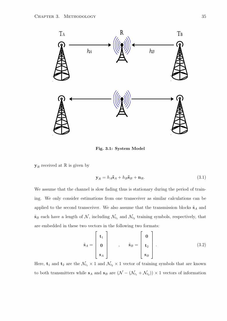
Chapter 3. Methodology 35
Fig. 3.1: System Model
yR received at R is given by
yR = hAsA + hB sB + nR. (3.1)
We assume that the channel is slow fading thus is stationary during the period of train-
ing. We only consider estimations from one transceiver as similar calculations can be
applied to the second transceiver. We also assume that the transmission blocks sA and
sB each have a length of N , including Nt1 and Nt2 training symbols, respectively, that
are embedded in these two vectors in the following two formats:
sA =
t1
0
sA
, sB =
0
t2
sB
. (3.2)
Here, t1 and t2 are the Nt1 × 1 and Nt2 × 1 vector of training symbols that are known
to both transmitters while sA and sB are (N − (Nt1 +Nt2)) × 1 vectors of information
Chapter 3. Methodology 36
symbols transmitted by TA and TB, respectively.
We define Pt1 , 1Nt1
tH1 t1 and Pt2 , 1Nt2
tH2 t2 as the power allocated to training at termi-
nals TA and TB, respectively.
The relay multiplies the received signal yR by a complex weight w and retransmits the
so-obtained signals. The complex weight w is evaluated as
√Pr
P1σ2hA
+ P2σ2hB
+ σ2r
(3.3)
where Pr is the power at the relay node, Pi, for i = {1, 2}, are the powers at TA and
TB, respectively and σ2hA, σ2
hBand σ2
r are the noise variances of hA, hB and the relay
respectively. This choice of w will ensure that the relay power at the relay is maintained
at Pr.
At TA, the vector of received signal corresponding to the first Nt1 +Nt2 symbol periods
is given by:
y1 = wh2At1 + whAn1 + n1A (3.4)
y2 = whAhBt2 + whAn2 + n2A . (3.5)
Assuming that the noise vectors n1, n1A, n2, and n2A are zero-mean unit-variance Gaus-
sian random vectors and that they are mutually independent, the conditional pdf of the
vector y = [yT1 yT
2 ]T is given by
f(y|w, hA, hB) =1
(2πσ2(hA))Nt1
+Nt22
exp
(−∥ y− µ(hA, hB) ∥2
2σ2(hA)
)(3.6)
where the mean vector is given by µ(hA, hB) , [µT1 (hA) µT
2 (hA, hB)]T , [wh2
AtT1 whAhBt
T2 ]
T
and the variance is expressed as
σ2(hA) = 1 + |whA|2. (3.7)

Chapter 3. Methodology 37
3.2 The ML Estimator
The channel coefficients hA and hB can be jointly estimated, using the ML approach, as
{hA, hB} = arg maxhA,hB
f(y|w, hA, hB) (3.8)
or equivalently as
{hA, hB} = arg maxhA,hB
ln f(y|w, hA, hB). (3.9)
To express hB in terms of hA, we take the derivative of the log-likelihood function
ln f(y|w, hA, hB) with respect to h∗B and equate it to zero. Given that
ln f(y|w, hA, hB) = −Nt1 +Nt2
2ln(2π)− Nt1 +Nt2
2lnσ2(hA)−
∥ y− µ(hA, hB) ∥2
2σ2(hA)
(3.10)
we can write (3.10) as
∂ ln f(y|w, hA, hB)
∂h∗B
= − 1
2σ2(hA)
∂
∂h∗B
(∥ y− µ(hA, hB) ∥2
)=
1
2σ2(hA)
∂
∂h∗B
((y− µ(hA, hB))
H(y− µ(hA, hB)))
= − 1
2σ2(hA)
∂µH(hA, hB)
∂h∗B
(y− µ(hA, hB))
= − 1
2σ2(hA)
[∂µH
1 (hA)
∂h∗B
(y1 − µ1(hA)) +∂µH
2 (hA, hB)
∂h∗B
(y2 − µ2(hA, hB))
]= − 1
2σ2(hA)(tH2 w
∗h∗A)(y2 − whAhBt2). (3.11)
We obtain an expression for hB in terms of hA by equating (3.11) to zero
hB =tH2 y2
Nt2 whAPt2
. (3.12)
Inserting (3.12) into (3.8) leads us to the following ML estimate for hA.
hA = argmaxhA
f(y|w, hA,tH2 y2
Nt2 whAPt2
). (3.13)

Chapter 3. Methodology 38
We can write
ln f(y|w, hA,tH2 y2
Nt2 whAPt2
) =− Nt1 +Nt2
2ln(2π)− Nt1 +Nt2
2lnσ2(hA)
− 1
2σ2(hA)
∥∥∥∥y− µ
(hA,
tHy2
Nt whAPt
)∥∥∥∥2
=− Nt1 +Nt2
2ln(2π)− Nt1 +Nt2
2lnσ2(hA)
− 1
2σ2(hA)∥ y1 − µ1(hA) ∥2
− 1
2σ2(hA)
∥∥∥∥y2 − µ2
(hA,
tH2 y2
Nt2 whAPt2
)∥∥∥∥2
(3.14)
where
µ2
(hA,
tH2 y2
Nt2 whAPt2
)= whA
(tH2 y2
Nt2 whAPt2
)t2 =
(tH2 y2
Nt2Pt2
)t2. (3.15)
Therefore, only the second and the third terms in (3.14) depend on hA. Let hA = αAejϕA
where αA and ϕA are the magnitude and phase of the complex channel hA , respectively.
Note that as σ2(hA) = (1+ |whA|2) = σ2(αA), then only the third term in (3.14) depends
on ϕA. Hence, we can write (3.14) as,
∂
∂ϕA
ln f(y|w, hA,tH2 y2
Nt2 whAPt2
) = − 1
2σ2(αA)
∂
∂ϕA
∥ y1 − µ1(hA)∥2
= − 1
2σ2(αA)
∂
∂ϕA
(∥y1∥2 − 2Re(yH1 µ1(hA)) + ∥µ1(hA)∥2)
=1
σ2(αA)
∂
∂ϕA
(Re(yH1 µ1(hA)))
=1
σ2(αA)
∂
∂ϕA
(Re(wα2Ae
j2ϕAyH1 t1))
=2α2
A
σ2(αA)(Re(jwej2ϕAyH
1 t1))
= − 2α2A
σ2(αA)(Im(wej2ϕAyH
1 t1)) (3.16)
Equating (3.16) to zero implies wej2ϕAyH1 t1 should be a real number. This requires
]w + 2ϕA + ]yH1 t1 = 2kπ (3.17)

Chapter 3. Methodology 39
where k is an integer. As a result, the estimate of ϕA is given by
ϕA = −1
2]wyH
1 t1 + kπ. (3.18)
An intrinsic ambiguity in the phase hA is observed as a result of the added value of kπ.
However, the product of the individual channels (h2A and hAhB) is what is required for
symbol detection at the transceivers (see equations (3.4) and (3.5)). Therefore, if an
instance of hA and hB is given by
hA1 = αAejϕA and hB1 = αBe
jϕB
and a second instance is given by
hA2 = αAej(ϕA+π) and hB2 = αBe
j(ϕB−π)
Then it can be shown that
h2A1
= α2Ae
2jϕ = h2A2
and
hA1hB1 = αAαBejϕAejϕB = hA2hB2 . (3.19)
From equation (3.19), it is observed that the product of the individual channels, (hA and
hB), without a shift in phase gives the same result as the product obtained when the
phase is shifted.
The estimate αA is found by taking the derivative of the log-likelihood function
ln f(y∣∣∣w,αAe
jϕA ,tH2 y2
Nt2 whAPt2
)with respect to αA.
∂
∂αA
ln f
(y
∣∣∣∣w, αAejϕA ,
tH2 y2
Nt2 whAPt2
)=
− (Nt1 +Nt2)
2σ2(αA)
∂σ2(αA)
∂αA
− 1
2σ4(αA)
(σ2(hA)
∂ ∥ y1 − µ1(αAejϕA) ∥
∂αA
2
− ∥ y1 − µ1(αAejϕA) ∥2 ∂σ2(αA)
∂αA
)− 1
2σ4(αA)
(σ2(hA)
∂ ∥ y2 − µ2 ∥∂αA
2
− ∥ y2 − µ2 ∥2∂σ2(αA)
∂αA
). (3.20)

Chapter 3. Methodology 40
Note that ∥ y1 − µ1(αAejϕA) ∥2= yH
1 y1 − 2α2A|wyH
1 t1| + Nt1 |w|2α4APt1 . Then, we can
write
∂ ∥ y1 − µ1(αAejϕA) ∥
∂αA
2
= −4αA|wyH1 t1|+ 4Nt1 |w|2α3
APt1 (3.21)
∂ ∥ y2 − µ2 ∥∂αA
2
= 0 (3.22)
We can also write
∂σ2(αA)
∂αA
= 2|w|2αA. (3.23)
Substituting (3.21), (3.22) and (3.23) into (3.20), and equating it to zero, we obtain the
optimal value of αA as the solution to the following equations:
− (Nt1 +Nt2)
2σ2(αA)(2|w|2αA)
− 1
2σ4(αA)
[σ2(αA)(−4αA|wyH
1 t1|+ 4|w|2α3ANt1 Pt1)
− (yH1 y1 − 2α2
A|wyH1 t1|+ |w|2α4
ANt1 Pt1)(2|w|2αA)]
− 1
2σ4(αA)
[σ2(αA)(0)− (∥ y2 − µ2 ∥2)(2|w|2αA)
]= 0 (3.24)
or
− Nt1 |w|2αA
σ2(αA)− Nt2 |w|2αA
σ2(αA)+
2|wyH1 t1|αA
σ2(αA)− 2|w|2Pt1α
3A
σ2(αA)+
yH1 y1|w|2αA
σ4(αA)− 2|wyH
1 t1||w|2α3A
σ4(αA)
+|w|4Nt1Pt1α
5A
σ4(αA)+∥ y2 − µ2 ∥2 |w|2αA
σ4(αA)= 0 (3.25)
Multiplying (3.25) by σ4(αA)αA
and using the fact that σ2(αA) = 1+ |wαA|2, we can simplify
(3.25) as
−Nt1 |w|2σ2(αA)−Nt2 |w|2σ2(αA) + 2|wyH1 t1|σ2(hA)− 2Nt1 |w|2Pt1σ
2(αA)α2A + yH
1 y1|w|2
− 2|w3yH1 t1|α2
A +Nt1 Pt1 |w|4α4A+ ∥ y2 − µ2 ∥2 |w|2 = 0 (3.26)
or as
−Nt1 |w|2 −Nt2 |w|2 −Nt1 |w|4α2A −Nt2 |w|4α2
A + 2|wyH1 t1|+ 2|w3yH
1 t1|α2A − 2Nt1 |w|2α2
APt1
− 2Nt1 |w|4α4APt + yH
1 y1|w|2 − 2|w3yH1 t1|α2
A +Nt1 |w|4Ptα4A+ ∥ y2 − µ2 ∥2 |w|2 = 0
(3.27)
Chapter 3. Methodology 41
or
−Nt1 Pt1 |w|4α4A −Nt1 |w|4α2
A −Nt2 |w|4α2A − 2Nt1 Pt1 |w|2α2
A −Nt1 |w|2 −Nt2 |w|2 + 2|wyH1 t1|
+ yH1 y1|w|2+ ∥ y2 − µ2 ∥2 |w|2 = 0. (3.28)
Equation (3.28) can be solved using the biquadratic equation,
αA =
√−b+
√b2 − 4ac
2a(3.29)
where (3.28) is represented by aα4A + bα2
A + c = 0 and the coefficients a, b, c are:
a = Nt1 Pt1 |w|4
b = |w|2(Nt1|w|2 +Nt2 |w|2 + 2Pt1Nt1)
c = Nt1 |w|2 +Nt2 |w|2 − 2|wyH1 t1| − yH
1 y1|w|2− ∥ y2 − µ2 ∥2 |w|2.
The estimates are finally expressed as
hA = αAejϕA (3.30)
hB =tH2 y2
Nt2 whAPt2
. (3.31)
We evaluate the performance of the hB by observing its mean and variance;
hB =tH2 (whAhBt2 + whAn2 + n2A)
Nt2 whAPt2
=tH2 t2whAhB
Nt2 whAPt2
+tH2 whAn2
Nt2 whAPt2
+tH2 n2A
Nt2 whAPt2
=hAhB
hA
+tH2 hAn2
Nt2 hAPt2
+tH2 n2A
Nt2 whAPt2︸ ︷︷ ︸noise
. (3.32)
From equation (3.32), it can be observed that some bias will be introduced to the estimate
hB as a result of errors in the estimate of hA.

Chapter 4
Assessment
This Section discusses numerical simulations carried out on the described network under
different transmission conditions. The proposed network consists of one relay node and
the channels hA and hB are complex zero-mean Gaussian random variables with variances
σ2hA
and σ2hB
respectively. The quality of the channel coefficients are measured by σ2hA
and σ2hB.
We examine the validity of the obtained results by observing the MSE of the obtained es-
timates. We consider the performance of the obtained estimates for a range of transceiver
powers P1 and P2 of TA and TB respectively, and relay power Pr all set at 0− 30 dBW
with increments of 10 dBW. We grid the values of Nt1 and Nt2 from 5 to 20 with steps
of 5. The training symbols are considered to be drawn from a QPSK constellation.
For different values of Nt1 and Nt2 we solve the ML problem of equation (3.8) and obtain
the estimates of the magnitude αA and phase ϕ of the the channel estimates hA. We then
use this estimate to solve for hB. We also observe the effects of changes in transceiver
and relay powers on the obtained estimates.
From Figs. 4.1 to 4.7, we analyze the behavior of the estimates of hA using different
training lengths and relay powers.
42

Chapter 4. Assessment 43
4.1 MSE of hA versus P1
Fig. 4.1 shows the plots of the MSE of hA versus P1 for different values of training
0 5 10 15 20 25 30
−70
−60
−50
−40
−30
−20
−10
0
P1(dBW)
MS
E h
A
Nt2 = 5 P2 = 30dBW Nt1 = 5Nt2 = 5 P2 = 30dBW Nt1 = 10Nt2 = 5 P2 = 30dBW Nt1 = 15Nt2 = 5 P2 = 30dBW Nt1 = 20
Fig. 4.1: MSE of hA versus P1 for varying training lengths of Nt1 and Nt2 = 5
symbols TA, Nt1 , and for Nt2 = 5 , P2 = 30dBW , and Pr = 30dBW. The plots show
that as the number of training symbols (Nt1) increase, the MSE of hA decreases. Also
MSE of hA is seen to decrease as P1 rises and produces a power gain of about 2dBW for
each increment of Nt1 .
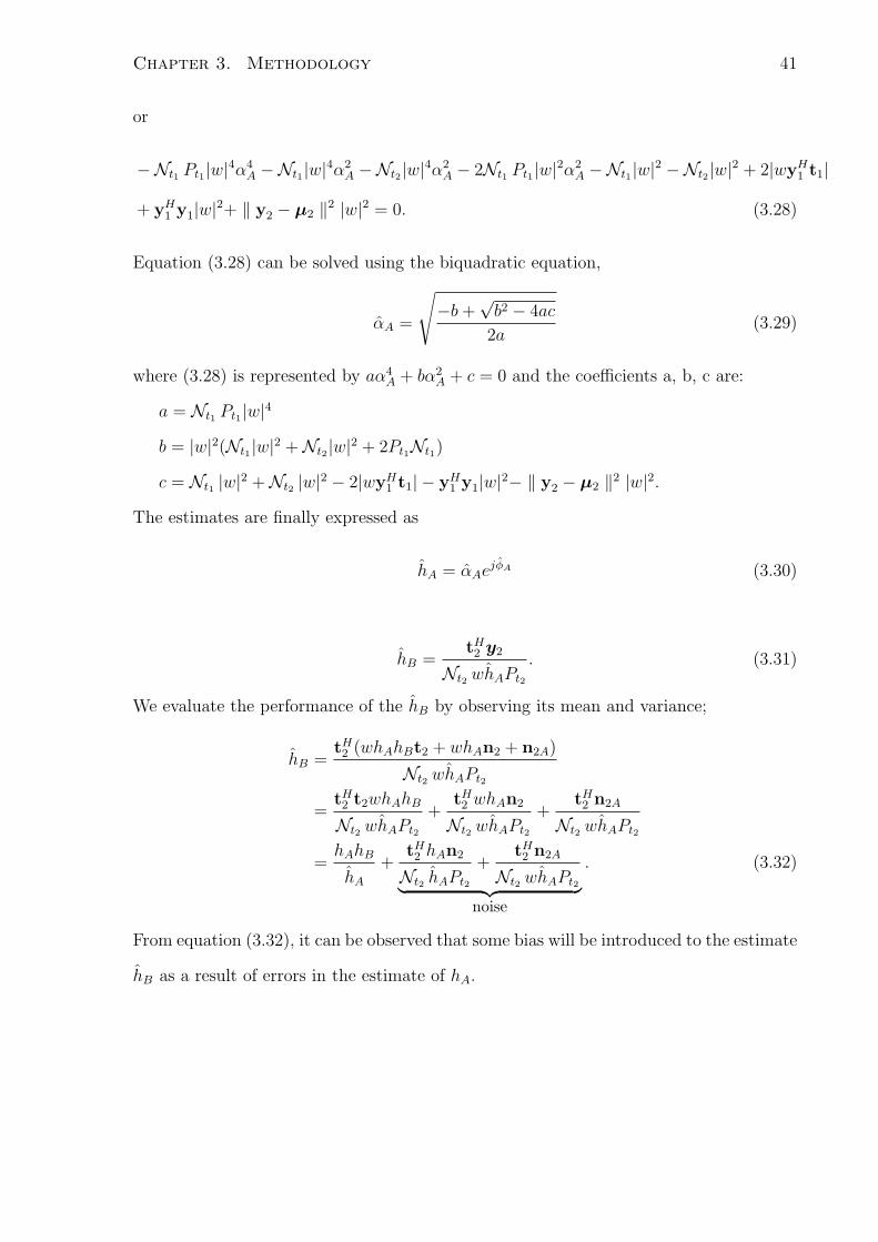
Fig. 4.2 shows the same axes values as in Fig. 4.1 but for increased value of Nt2 = 20. P2
and Pr remain fixed at 30 dBW. A slight decrease in the MSE of hA is observed resulting
in a power gain of 0.1dBW when compared to Fig. 4.2. This is because the value of
the power and length of training from TB has very little impact on the outcome of the
estimate hA.
Fig. 4.3 depicts the result of increases in the training lengths used by TB on the estimate
of the channel hA. As observed, the changes in MSE are quite minimal and only evident
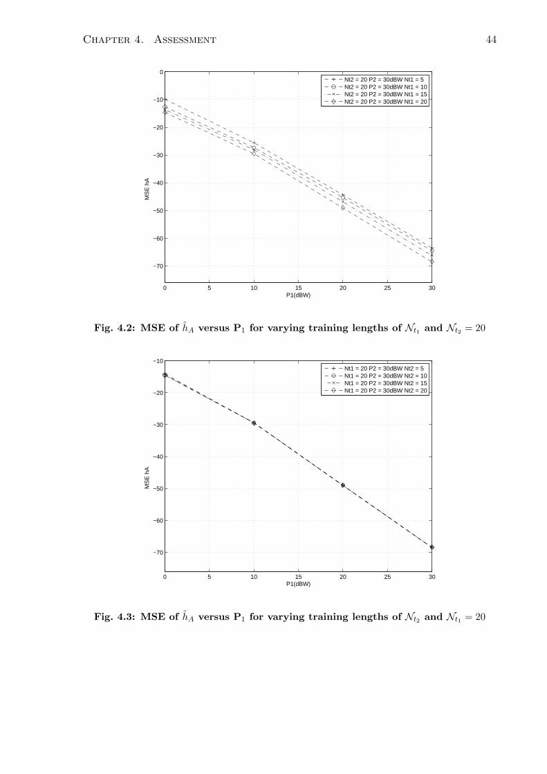
Chapter 4. Assessment 44
0 5 10 15 20 25 30
−70
−60
−50
−40
−30
−20
−10
0
P1(dBW)
MS
E h
A
Nt2 = 20 P2 = 30dBW Nt1 = 5Nt2 = 20 P2 = 30dBW Nt1 = 10Nt2 = 20 P2 = 30dBW Nt1 = 15Nt2 = 20 P2 = 30dBW Nt1 = 20
Fig. 4.2: MSE of hA versus P1 for varying training lengths of Nt1 and Nt2 = 20
0 5 10 15 20 25 30
−70
−60
−50
−40
−30
−20
−10
P1(dBW)
MS
E h
A
Nt1 = 20 P2 = 30dBW Nt2 = 5Nt1 = 20 P2 = 30dBW Nt2 = 10Nt1 = 20 P2 = 30dBW Nt2 = 15Nt1 = 20 P2 = 30dBW Nt2 = 20
Fig. 4.3: MSE of hA versus P1 for varying training lengths of Nt2 and Nt1 = 20
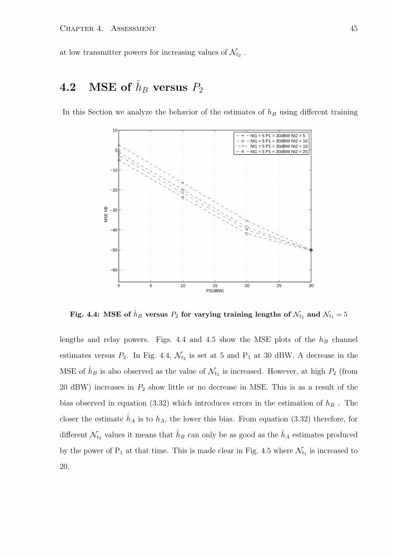
Chapter 4. Assessment 45
at low transmitter powers for increasing values of Nt2 .
4.2 MSE of hB versus P2
In this Section we analyze the behavior of the estimates of hB using different training
0 5 10 15 20 25 30
−60
−50
−40
−30
−20
−10
0
10
P2(dBW)
MS
E h
B
Nt1 = 5 P1 = 30dBW Nt2 = 5Nt1 = 5 P1 = 30dBW Nt2 = 10Nt1 = 5 P1 = 30dBW Nt2 = 15Nt1 = 5 P1 = 30dBW Nt2 = 20
Fig. 4.4: MSE of hB versus P2 for varying training lengths of Nt2 and Nt1 = 5
lengths and relay powers. Figs. 4.4 and 4.5 show the MSE plots of the hB channel
estimates versus P2. In Fig. 4.4, Nt2 is set at 5 and P1 at 30 dBW. A decrease in the
MSE of hB is also observed as the value of Nt2 is increased. However, at high P2 (from
20 dBW) increases in P2 show little or no decrease in MSE. This is as a result of the
bias observed in equation (3.32) which introduces errors in the estimation of hB . The
closer the estimate hA is to hA, the lower this bias. From equation (3.32) therefore, for
different Nt2 values it means that hB can only be as good as the hA estimates produced
by the power of P1 at that time. This is made clear in Fig. 4.5 where Nt1 is increased to
20.

Chapter 4. Assessment 46
0 5 10 15 20 25 30
−60
−50
−40
−30
−20
−10
0
10
P2(dBW)
MS
E h
B
Nt1 = 20 P1 = 30dBW Nt2 = 5Nt1 = 20 P1 = 30dBW Nt2 = 10Nt1 = 20 P1 = 30dBW Nt2 = 15Nt1 = 20 P1 = 30dBW Nt2 = 20
Fig. 4.5: MSE of hB versus P2 for varying Nt2 and Nt1 = 20
4.3 Performance of Estimator for for varying relay
power Pr
We also consider the effect of the complex weight w at the relay on the estimation of hA
and hB. Fig. 4.6 and 4.7 depicts the plots for increasing relay power Pr. In Fig. 4.6, Nt1
is set at 5 and MSE of hA is seen to continually decrease with increase in P1. Specifically,
an increment from 10 dBW to 20 dBW results in a power gain of 2dBW.
In Fig. 4.7, the number of training symbols Nt1 is increased to 20 and the MSE of hA is
observed to decrease by 5. These show the reliance of the estimator on the number of
training symbols sent from the transmitter where the estimation is carried out.
The curves in Figs. 4.8 and 4.9 show how relay power Pr affects hB. As depicted,
increasing relay power also improves the accuracy of the estimates. Also observed is that
an increase in Nt1 from 5 to 20 reduces the MSE of hB.

Chapter 4. Assessment 47
0 5 10 15 20 25 30
−70
−60
−50
−40
−30
−20
−10
0
P1(dBW)
MS
E h
A
Pr = 10dBW Nt1 = 5Pr = 20dBW Nt1 = 5Pr = 30dBW Nt1 = 5
Fig. 4.6: MSE of hA versus P1 for varying Pr and Nt1 = 5
0 5 10 15 20 25 30
−70
−60
−50
−40
−30
−20
−10
P1(dBW)
MS
E h
A
Pr = 10dBW Nt1 = 20Pr = 20dBW Nt1 = 20Pr = 30dBW Nt1 = 20
Fig. 4.7: MSE of hA versus P1 for varying Pr and Nt1 = 20

Chapter 4. Assessment 48
0 5 10 15 20 25 30
−50
−40
−30
−20
−10
0
10
P2(dBW)
MS
E h
B
Nt2 = 5 Pr = 10dBWNt2 = 5 Pr = 20dBWNt2 = 5 Pr = 30dBW
Fig. 4.8: MSE of hB versus P2 for varying relay power Pr and Nt2 = 5
0 5 10 15 20 25 30
−60
−50
−40
−30
−20
−10
0
P2(dBW)
MS
E h
B
Nt2 = 20 Pr = 10dBWNt2 = 20 Pr = 20dBWNt2 = 20 Pr = 30dBW
Fig. 4.9: MSE of hB versus P2 for varying relay power Pr and Nt2 = 20
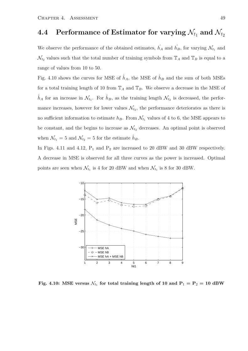
Chapter 4. Assessment 49
4.4 Performance of Estimator for varying Nt1 and Nt2
We observe the performance of the obtained estimates, hA and hB, for varying Nt1 and
Nt2 values such that the total number of training symbols from TA and TB is equal to a
range of values from 10 to 50.
Fig. 4.10 shows the curves for MSE of hA, the MSE of hB and the sum of both MSEs
for a total training length of 10 from TA and TB. We observe a decrease in the MSE of
hA for an increase in Nt1 . For hB, as the training length Nt2 is decreased, the perfor-
mance increases, however for lower values Nt2 , the performance deteriorates as there is
no sufficient information to estimate hB. From Nt1 values of 4 to 6, the MSE appears to
be constant, and the begins to increase as Nt2 decreases. An optimal point is observed
when Nt1 = 5 and Nt2 = 5 for the estimate hB.
In Figs. 4.11 and 4.12, P1 and P2 are increased to 20 dBW and 30 dBW respectively.
A decrease in MSE is observed for all three curves as the power is increased. Optimal
points are seen when Nt1 is 4 for 20 dBW and when Nt1 is 8 for 30 dBW.
1 2 3 4 5 6 7 8 9
−30
−25
−20
−15
−10
Nt1
MS
E
MSE hAMSE hBMSE hA + MSE hB
Fig. 4.10: MSE versus Nt1 for total training length of 10 and P1 = P2 = 10 dBW
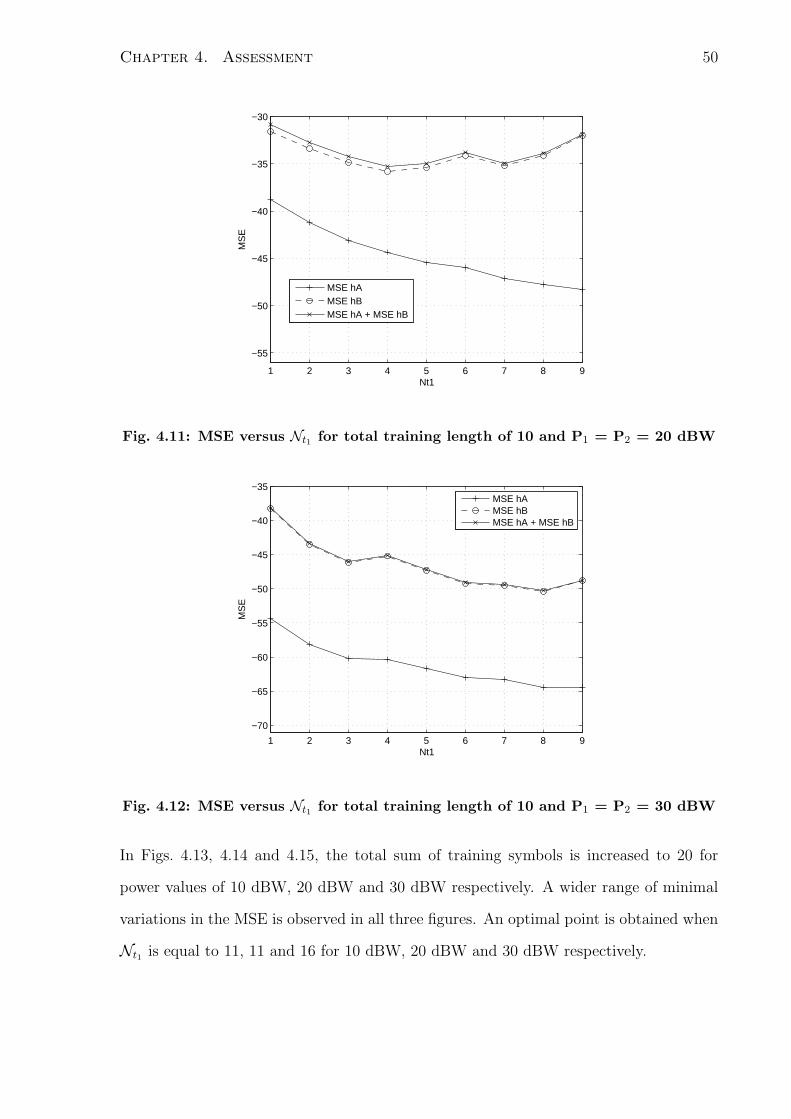
Chapter 4. Assessment 50
1 2 3 4 5 6 7 8 9
−55
−50
−45
−40
−35
−30
Nt1
MS
E
MSE hAMSE hBMSE hA + MSE hB
Fig. 4.11: MSE versus Nt1 for total training length of 10 and P1 = P2 = 20 dBW
1 2 3 4 5 6 7 8 9
−70
−65
−60
−55
−50
−45
−40
−35
Nt1
MS
E
MSE hAMSE hBMSE hA + MSE hB
Fig. 4.12: MSE versus Nt1 for total training length of 10 and P1 = P2 = 30 dBW
In Figs. 4.13, 4.14 and 4.15, the total sum of training symbols is increased to 20 for
power values of 10 dBW, 20 dBW and 30 dBW respectively. A wider range of minimal
variations in the MSE is observed in all three figures. An optimal point is obtained when
Nt1 is equal to 11, 11 and 16 for 10 dBW, 20 dBW and 30 dBW respectively.
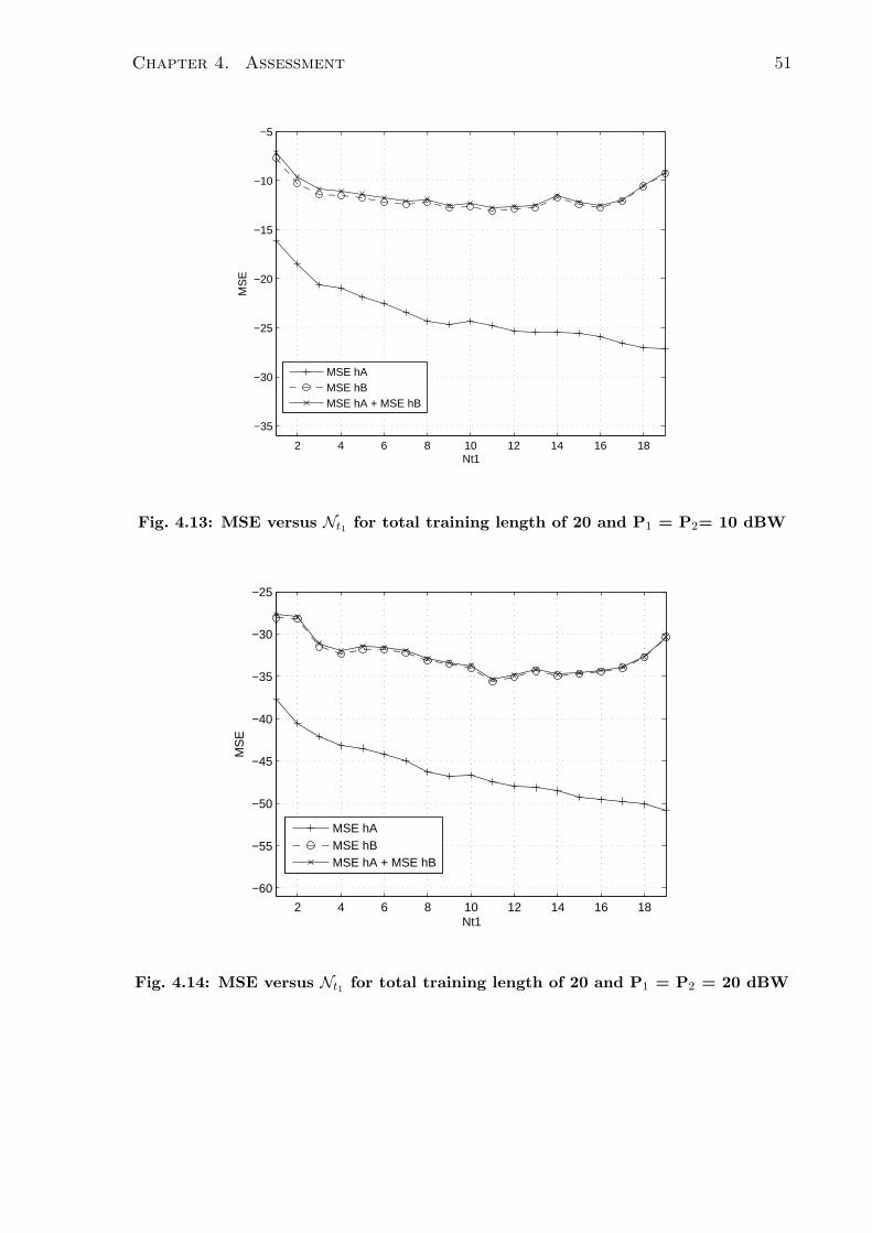
Chapter 4. Assessment 51
2 4 6 8 10 12 14 16 18
−35
−30
−25
−20
−15
−10
−5
Nt1
MS
E
MSE hAMSE hBMSE hA + MSE hB
Fig. 4.13: MSE versus Nt1 for total training length of 20 and P1 = P2= 10 dBW
2 4 6 8 10 12 14 16 18
−60
−55
−50
−45
−40
−35
−30
−25
Nt1
MS
E
MSE hAMSE hBMSE hA + MSE hB
Fig. 4.14: MSE versus Nt1 for total training length of 20 and P1 = P2 = 20 dBW
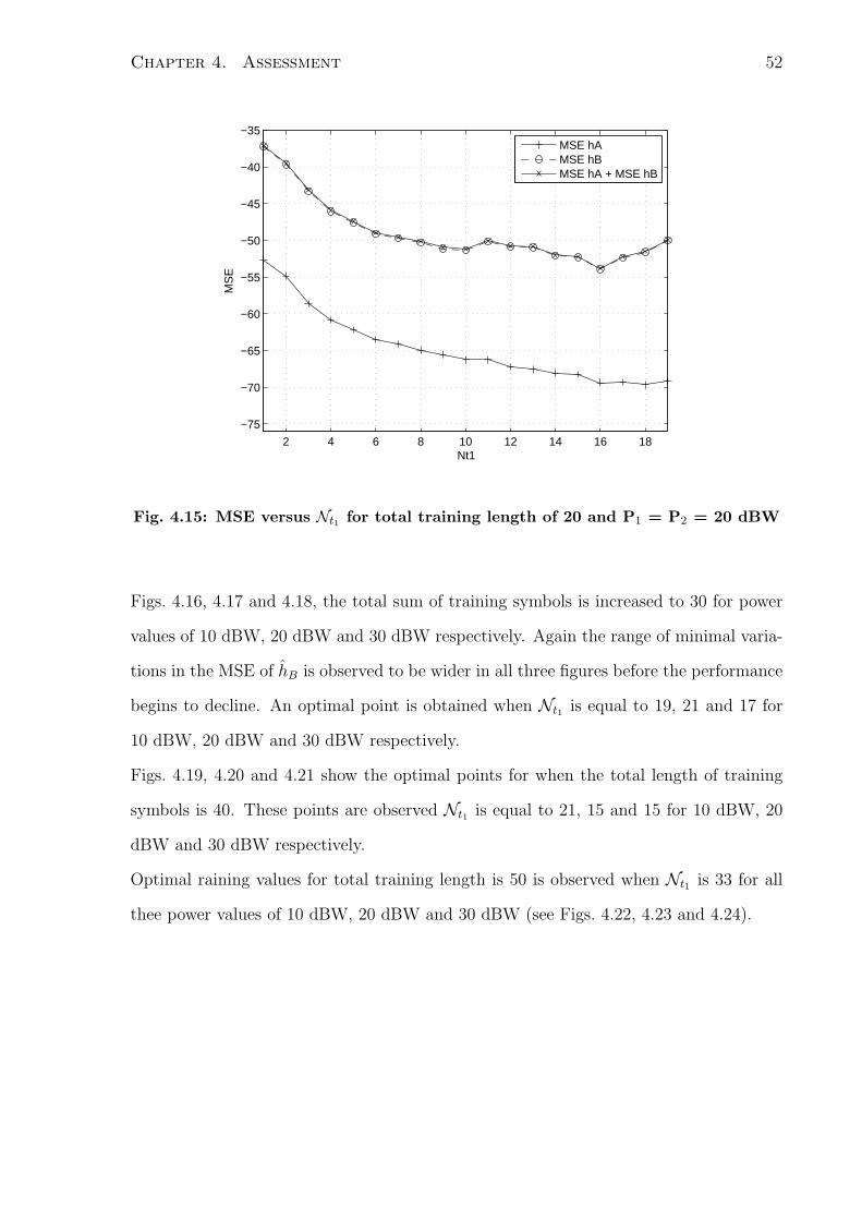
Chapter 4. Assessment 52
2 4 6 8 10 12 14 16 18
−75
−70
−65
−60
−55
−50
−45
−40
−35
Nt1
MS
E
MSE hAMSE hBMSE hA + MSE hB
Fig. 4.15: MSE versus Nt1 for total training length of 20 and P1 = P2 = 20 dBW
Figs. 4.16, 4.17 and 4.18, the total sum of training symbols is increased to 30 for power
values of 10 dBW, 20 dBW and 30 dBW respectively. Again the range of minimal varia-
tions in the MSE of hB is observed to be wider in all three figures before the performance
begins to decline. An optimal point is obtained when Nt1 is equal to 19, 21 and 17 for
10 dBW, 20 dBW and 30 dBW respectively.
Figs. 4.19, 4.20 and 4.21 show the optimal points for when the total length of training
symbols is 40. These points are observed Nt1 is equal to 21, 15 and 15 for 10 dBW, 20
dBW and 30 dBW respectively.
Optimal raining values for total training length is 50 is observed when Nt1 is 33 for all
thee power values of 10 dBW, 20 dBW and 30 dBW (see Figs. 4.22, 4.23 and 4.24).

Chapter 4. Assessment 53
5 10 15 20 25
−40
−35
−30
−25
−20
−15
−10
−5
Nt1
MS
E
MSE hAMSE hBMSE hA + MSE hB
Fig. 4.16: MSE versus Nt1 for total training length of 30 and P1 = P2 = 10 dBW
5 10 15 20 25
−55
−50
−45
−40
−35
−30
−25
−20
Nt1
MS
E
MSE hAMSE hBMSE hA + MSE hB
Fig. 4.17: MSE versus Nt1 for total training length of 30 and P1 = P2 = 20 dBW

Chapter 4. Assessment 54
5 10 15 20 25
−75
−70
−65
−60
−55
−50
−45
−40
−35
Nt1
MS
E
MSE hAMSE hBMSE hA + MSE hB
Fig. 4.18: MSE versus Nt1 for total training length of 30 and P1 = P2 = 30 dBW
5 10 15 20 25 30 35
−40
−35
−30
−25
−20
−15
−10
−5
Nt1
MS
E
MSE hAMSE hBMSE hA + MSE hB
Fig. 4.19: MSE versus Nt1 for total training length of 40 and P1 = P2= 10 dBW
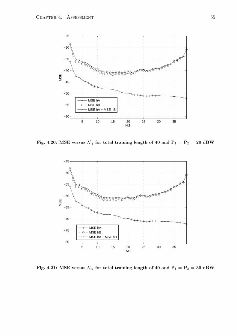
Chapter 4. Assessment 55
5 10 15 20 25 30 35
−60
−55
−50
−45
−40
−35
−30
−25
Nt1
MS
E
MSE hAMSE hBMSE hA + MSE hB
Fig. 4.20: MSE versus Nt1 for total training length of 40 and P1 = P2 = 20 dBW
5 10 15 20 25 30 35
−80
−75
−70
−65
−60
−55
−50
−45
Nt1
MS
E
MSE hAMSE hBMSE hA + MSE hB
Fig. 4.21: MSE versus Nt1 for total training length of 40 and P1 = P2 = 30 dBW
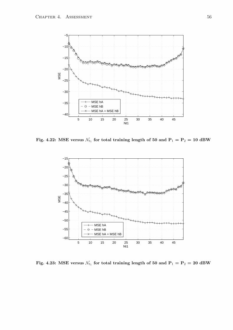
Chapter 4. Assessment 56
5 10 15 20 25 30 35 40 45
−40
−35
−30
−25
−20
−15
−10
−5
Nt1
MS
E
MSE hAMSE hBMSE hA + MSE hB
Fig. 4.22: MSE versus Nt1 for total training length of 50 and P1 = P2 = 10 dBW
5 10 15 20 25 30 35 40 45−60
−55
−50
−45
−40
−35
−30
−25
−20
−15
Nt1
MS
E
MSE hAMSE hBMSE hA + MSE hB
Fig. 4.23: MSE versus Nt1 for total training length of 50 and P1 = P2 = 20 dBW

Chapter 4. Assessment 57
5 10 15 20 25 30 35 40 45−80
−75
−70
−65
−60
−55
−50
−45
−40
−35
Nt1
MS
E
MSE hAMSE hBMSE hA + MSE hB
Fig. 4.24: MSE versus Nt1 for total training length of 50 and P1 = P2 = 30 dBW
4.5 Performance of Estimator for different channel
qualities
Figs. 4.25 to 4.27 show the performances of the estimator for different channel qualities.
The variance of hA, (σ2hA) is varied from values 0.5, 1 and 2 while that of hB, (σ
2hB), is
fixed at 1.
In Fig. 4.25, an optimal point is obtained when Nt1 = 13. Increasing σ2hA
to 1 means
the quality of both channels hA and hB are the same and results a slight increase in the
performance of the estimates (Fig. 4.26). For this condition, an optimal point is obtained
for Nt1 = 8. In Fig. 4.26, σ2hA
is equal to 2 and the optimal training length is observed
when Nt1 is 12.

Chapter 4. Assessment 58
2 4 6 8 10 12 14 16 18
−35
−30
−25
−20
−15
−10
−5
0
Nt1
MS
E
MSE hAMSE hBMSE hA + MSE hB
Fig. 4.25: MSE versus Nt1 for σ2hA
= 0.5 , σ2hB
= 1 and P1 = P2 = 10 dBW
2 4 6 8 10 12 14 16 18
−35
−30
−25
−20
−15
−10
−5
Nt1
MS
E
MSE hAMSE hBMSE hA + MSE hB
Fig. 4.26: MSE versus Nt1 for σ2hA
= 1, σ2hB
= 1 and P1 = P2 = 10 dBW

Chapter 4. Assessment 59
2 4 6 8 10 12 14 16 18
−35
−30
−25
−20
−15
−10
−5
Nt1
MS
E
MSE hAMSE hBMSE hA + MSE hB
Fig. 4.27: MSE versus Nt1 for σ2hA
= 2 , σ2hB
= 1 and P1 = P2 = 10 dBW

Chapter 5
Conclusion
In this thesis, we studied channel estimation in a two-way relay network for different
numbers of training symbols at the transceivers. Our system model comprises of two
single antenna transceivers communicating through one relay node which is also equipped
with one antenna. The transmission of data is accomplished in two phases. During the
first phase both transceivers transmit their data which is embedded with known training
symbols to the relay. The relay amplifies the combined received signal by multiplying
with a complex weight before retransmitting to both transceivers in the second phase.
Our goal is to estimate the channels connecting this network using the MLE and compare
their performance for different lengths of training symbols. Estimation was carried out
and simulated from one of the transceivers as a similar argument can be made for the
other. To solve the likelihood equation, we first obtained an expression for far channel in
terms of the near channel. We then obtained the estimate of the phase and amplitude of
the near channel. The obtained estimate is then used to determine the estimate of the
far channel.
Our simulations show continued improvements of the estimates as the training lengths
from the transceiver under consideration increases. However, increasing the number of
training symbols from the distant transceiver results in minimal improvements in the
60
Chapter 5. Conclusion 61
MSE of the computed estimates. Furthermore, the accuracy of the estimates of the far
channel is large influenced by the accuracy of the estimates of the near channel. Optimal
training lengths were obtained for different power values as well.
We also considered the effects of relay power on the channel coefficient estimates. Results
obtained show decreases in MSE of the obtained estimates as the relay power is increased.
Simulations also showed that for different channel qualities, increasing the length of
training from the near transceiver yields a better performance. However the performance
of the distant channel declines as the training symbols from the distant transceivers
decreases significantly.
Compared to other surveyed research on channel estimation in two way relay networks,
this thesis differs in its use of varying training symbol lengths from the near and distant
transceivers. This variation is useful in situations where one of the channel is stronger
than the other.
As research in two–way relay networks gain more interest, the need for channel estimation
in such networks required for coherent detection increases. Thus the theories discussed
in this thesis could be applied.
5.1 Future work
In this thesis we considered channel estimation where the training symbols are used.
Although this is a less computationally intense approach, it is however also less bandwidth
efficient. For increase in accuracy of the channel estimates, a reasonable amount of the
allocated bandwidth has to be used for training. Therefore the blind estimation technique
could be applied to improve bandwidth efficiency.
References
[1] D. Tse, Fundamentals of Wireless Communications. New York: Cambridge Uni-
versity Press, 2004.
[2] W. S. K.J. Ray Liu, A.K Sadek and A. Kwasinski, Cooperative Communications and
Networking. Cambridge, 2009.
[3] T. Rappaport, Wireless Communications: Principles and Practice. Prentice Hall,
2001.
[4] S. Diggavi, N. Al-Dhahir, A. Stamoulis, and A. Calderbank, “Great expectations:
the value of spatial diversity in wireless networks,” Proceedings of the IEEE, vol. 92,
pp. 219–270, Feb. 2004.
[5] A. Goldsmith, Wireless Communications. New York: Cambridge University Press,
2005.
[6] A. Sendonaris, E. Erkip, and B. Aazhang, “User cooperation diversity - Part I:
System description,” IEEE Transactions on Communications, vol. 51, no. 11, pp.
1927–1938, Nov. 2003.
[7] ——, “User cooperation diversity - Part II: Implementation aspects and performance
analysis,” IEEE Transactions on Communications, vol. 51, no. 11, pp. 1939–1948,
Nov. 2003.
62

References 63
[8] A. Nosratinia, T. E. Hunter, and A. Hedayat, “Cooperative communication in wire-
less networks,” IEEE Communications Magazine, vol. 42, no. 10, pp. 74–80, Oct.
2004.
[9] C. E. Shannon, “Two-way communication channels,” in Proc. 4th Berkeley Symp.
Math., Statist. Probab., vol. 1, pp. 611–644, 1961.
[10] V. Havary-Nassab, S. Shahbazpanahi, and A. Grami, “Optimal distributed beam-
forming for two-way relay networks,” IEEE Transactions on Signal Processing,
vol. 58, no. 3, pp. 1238–1250, Mar. 2010.
[11] T. Ferrett, M. C. Valenti, and D. Torrieri, “Receiver design for noncoherent digital
network coding,” Military Communications Conference (MILCOM), 2010.
[12] S. M. Kay, Fundamentals of Statistical Signal Processing: Estimation Theory. New
Jersey: Prentice-Hall, 1993.
[13] I. J. Myung, “Tutorial on maximum likelihood estimation,” Journal of Mathematical
Psychology, pp. 90–100, Nov. 2001.
[14] J. K. Tugnait, L. Tong, and Z. Ding, “Single-user channel estimation and equaliza-
tion,” IEEE Signal Processing Magazine, vol. 17, no. 3, May 2000.
[15] J. N. Laneman, D. N. C. Tse, and G. W. Wornell, “Cooperative diversity in wireless
networks: Efficient protocols and outage behavior,” IEEE Transactions on Infor-
mation Theory, vol. 50, no. 12, pp. 3062–3080, Dec. 2004.
[16] A. Bletsas, A. Khisti, D. P. Reed, and A. Lippman, “A simple cooperative diver-
sity method based on network path selection,” IEEE Journal on Selected Areas in
Communications, vol. 24, no. 3, pp. 659–672, Mar. 2006.
References 64
[17] Y. Zhao, R. Adve, and T. J. Lim, “Improving amplify-and-forward relay networks:
Optimal power allocation versus selection,” IEEE International Symposium on In-
formation Theory, pp. 1234–1238, Jul. 2006.
[18] Y.-W. Hong, W. J. Huang, F.-H. Chiu, and C. C. J. Kuo, “Cooperative communica-
tions in resource-constrained wireless networks,” IEEE Signal Processing Magazine,
vol. 24, no. 3, pp. 47–57, Aug. 2002.
[19] B. Rankov and A. Wittneben, “Spectral efficient signaling for half-duplex relay chan-
nels,” Thirty-Ninth Asilomar Conference on Signals, Systems and Computers, pp.
1066–1071, Nov. 2005.
[20] M. Chen and A. Yener, “Power allocation for multi-access two-way relaying,” IEEE
International Conference on Communications (ICC), pp. 1–5, Jun. 2009.
[21] K.-S. Hwang, Y.-C. Ko, and M.-S. Alouini, “Performance bounds for two-way
amplify-and-forward relaying based on relay path selection,” IEEE 69th Vehicular
Technology Conference (VTC), pp. 1550–2252, 2009.
[22] V. Havary-Nassab, S. Shahbazpanahi, and A. Grami, “General-rank beamforming
for multi-antenna relaying schemes,” IEEE International Conference on Communi-
cations (ICC), pp. 1–5, Jun. 2009.
[23] B. Gedik and M. Uysal, “Two channel estimation methods for amplify-and-forward
relay networks,” Canadian Conference on Electrical and Computer Engineering
(CCECE), pp. 000 615–000 618, May 2008.
[24] A. S. Lalos, A. A. Rontogiannis, and K. Berberidis, “Channel estimation techniques
in amplify and forward relay networks,” in IEEE 9th Workshop on Signal Processing
Advances in Wireless Communications (SPAWC), Jul. 2008.

References 65
[25] Y. Yan, G. M. Gye Mun Jo, S. Balakannan, and M. H. Lee, “Joint channel estimation
in asynchronous amplify-and-forward relay networks based on ofdm signaling,” 9th
International Symposium on Communications and Information Technology (ISCIT),
p. 871, Sept. 2009.
[26] H. Yomo and E. de Carvalho, “A CSI estimation method for wireless relay network,”
IEEE Communications Letters, vol. 11, no. 6, Jul. 2007.
[27] A. S. Behbahani and A. Eltawil, “On channel estimation and capacity for am-
plify and forward relay networks,” IEEE Global Telecommunications Conference
(GLOBECOM), pp. 1–5, Dec. 2008.
[28] S. Sun and Y. Jing, “Channel training and estimation in distributed space-time
coded relay networks with multiple transmit/receive antennas,” 2010 IEEE Wireless
Communications and Networking Conference (WCNC), pp. 1525–3511, 2010.
[29] J. Zhao, M. Kuhn, A. Wittneben, and G. Bauch, “Self-interference aided channel
estimation in two-way relaying systems,” in IEEE Global Telecommunications Con-
ference (GLOBECOM), 2008.
[30] Y. Jia and A. Vosoughi, “Impact of channel estimation error upon sum-rate in
amplify-and-forward two-way relaying systems,” IEEE Eleventh International Work-
shop on Signal Processing Advances in Wireless Communications (SPAWC), 2010.
[31] F. Gao, R. Zhang, and Y.-C. Liang, “Channel estimation for OFDM modulated
two-way relay networks,” IEEE Transactions on Signal Processing, vol. 57, no. 11,
pp. 4443–4455, Nov. 2009.
[32] B. Jiang, F. Gao, X. Gao, and A. Nallanathan, “Channel estimation for amplify-
and-forward two-way relay network with power allocation,” in IEEE International
Conference on Communications (ICC), 2009.
References 66
[33] S. Abdallah and I. Psaromiligkos, “Blind channel estimation for mpsk-based amplify-
and-forward two-way relaying,” in 36th International Conference on Acoustics,
Speech and Signal Processing at the Prague Congress Centre (PCC), May 2011.
[34] F. Gao, R. Zhang, and Y.-C. Liang, “On channel estimation for amplify-and-forward
two-way relay networks,” in IEEE Global Telecommunications Conference. GLOBE-
COM 2008., New Orleans, LO, Dec. 2008.
[35] ——, “Optimal channel estimation and training design for two-way relay networks,”
IEEE Transactions on Communications, vol. 57, no. 10, pp. 3024–3033, Oct. 2009.
Related Documents