Channel Characteristics and Receiver Performance Analysis ...

University of Calgary

PRISM: University of Calgary's Digital Repository

Graduate Studies The Vault: Electronic Theses and Dissertations

2019-08-02

Channel Characteristics and Receiver Performance

Analysis of Mud Pulse Telemetry System

Nath, Santosh

Nath, S. (2019). Channel Characteristics and Receiver Performance Analysis of Mud Pulse

Telemetry System (Unpublished master's thesis). University of Calgary, Calgary, AB.

http://hdl.handle.net/1880/110698

master thesis

University of Calgary graduate students retain copyright ownership and moral rights for their

thesis. You may use this material in any way that is permitted by the Copyright Act or through

licensing that has been assigned to the document. For uses that are not allowable under

copyright legislation or licensing, you are required to seek permission.

Downloaded from PRISM: https://prism.ucalgary.ca

UNIVERSITY OF CALGARY

Channel Characteristics and Receiver Performance Analysis of Mud Pulse Telemetry

System

by

Santosh Nath

A THESIS

SUBMITTED TO THE FACULTY OF GRADUATE STUDIES

IN PARTIAL FULFILMENT OF THE REQUIREMENTS FOR THE

DEGREE OF MASTER OF SCIENCE

GRADUATE PROGRAM IN ELECTRICAL ENGINEERING

CALGARY, ALBERTA

AUGUST, 2019

c©Santosh Nath 2019

Abstract

Improving the data rate has been a major challenge in mud pulse telemetry. One of

the reasons for the confinement in lower data rate is due to the lack of knowledge of the mud

communication channel. Furthermore, the mud property, drill string geometry, interferers

from the mud pumps and noise affect the pressure wave propagation.

This thesis provides a novel mathematical characterization of a mud communication

channel and uses several signal processing techniques to enhance the performance of a mud

pulse receiver. By introducing a fluid transmission line model, the attenuation of the pressure

wave is characterised and is verified with the experimental results found in the literature.

Based on this model, a transfer function of the mud communication channel including the

effect of reflections from the multiple junctions has been derived. Finally, the receiver per-

formance is evaluated by cancelling out the narrow-band interferers and equalizing the mud

channel.

ii

Preface

This thesis is submitted for the degree of Master of Science at the University of Calgary. The

research described in this thesis was completed under the supervision of Professor Geoffrey

Messier and co-supervision of Professor Leonid Belostotski in the Department of Electrical

and Computer Engineering.

To the best of my knowledge, this work is original. All the previous works and experimental

data discussed and used in this thesis are duly acknowledged and referenced. No part of this

thesis has been previously published.

iii

Acknowledgements

I would like to extend my sincere thanks to my supervisor Professor Geoffrey Messier and

co-supervisor Professor Leonid Belostotski in the Department of Electrical and Computer

Engineering under the guidance of whom this work was completed. I appreciate their pro-

fessional mentorship, valuable ideas and endless support throughout the completion of this

thesis.

I would like to thank Dr. Roman Shor, Assistant Professor in the Department of Chemical

and Petroleum Engineering at Schulich School of Engineering and Derek Belle, Lead En-

gineer at MWDPlanet Calgary, for their valuable advice and ideas in the beginning of the

research.

Sincere thanks are extended to Professors and staffs in the Department of Electrical and Com-

puter Engineering at Schulich School of Engineering and in particular to my co-members of

the FISH Laboratory for their support and cooperation during the completion of this thesis.

Finally, I take this opportunity to express my gratitude to my family and friends for their

encouragement and support throughout my academic endeavour.

iv

Contents

Abstract ii

Preface iii

Acknowledgements iv

List of Figures viii

List of Tables xi

Nomenclatures and Abbreviations xii

1 Introduction 1

1.1 Measurement while drilling . . . . . . . . . . . . . . . . . . . . . . . . . . . . 1

1.1.1 Acoustic telemetry . . . . . . . . . . . . . . . . . . . . . . . . . . . . 3

1.1.2 Wireline telemetry . . . . . . . . . . . . . . . . . . . . . . . . . . . . 3

1.1.3 Electromagnetic telemetry . . . . . . . . . . . . . . . . . . . . . . . . 3

1.1.4 Mud pulse telemetry . . . . . . . . . . . . . . . . . . . . . . . . . . . 4

1.1.5 Comparison of telemetry methods . . . . . . . . . . . . . . . . . . . . 5

1.2 Structure of a MWD communication system . . . . . . . . . . . . . . . . . . 6

1.2.1 Transmitter . . . . . . . . . . . . . . . . . . . . . . . . . . . . . . . . 6

1.2.2 Channel . . . . . . . . . . . . . . . . . . . . . . . . . . . . . . . . . . 6

1.2.3 Noise and interference . . . . . . . . . . . . . . . . . . . . . . . . . . 7

1.2.4 Receiver . . . . . . . . . . . . . . . . . . . . . . . . . . . . . . . . . . 7

1.3 Intersymbol interference and noise in a mud pulse communication system . . 9

v

1.4 Problem statement . . . . . . . . . . . . . . . . . . . . . . . . . . . . . . . . 10

1.5 Literature review . . . . . . . . . . . . . . . . . . . . . . . . . . . . . . . . . 12

1.6 Contribution of this research . . . . . . . . . . . . . . . . . . . . . . . . . . . 15

1.7 Organization of the thesis . . . . . . . . . . . . . . . . . . . . . . . . . . . . 17

2 Mud pulse communication system review 19

2.1 Overview of a mud pulse telemetry system . . . . . . . . . . . . . . . . . . . 19

2.1.1 Mud pulse communication system . . . . . . . . . . . . . . . . . . . . 20

2.2 Data rates in mud pulse telemetry . . . . . . . . . . . . . . . . . . . . . . . . 21

2.3 Mud pulse transmitter . . . . . . . . . . . . . . . . . . . . . . . . . . . . . . 23

2.3.1 Discrete Pulser . . . . . . . . . . . . . . . . . . . . . . . . . . . . . . 23

2.3.2 Continuous pulser . . . . . . . . . . . . . . . . . . . . . . . . . . . . . 25

2.4 Mud pulse channel . . . . . . . . . . . . . . . . . . . . . . . . . . . . . . . . 27

2.5 Noise in a mud pulse communication system . . . . . . . . . . . . . . . . . . 29

2.5.1 Wide-band thermal noise . . . . . . . . . . . . . . . . . . . . . . . . . 30

2.5.2 Narrow-band mud pump noise . . . . . . . . . . . . . . . . . . . . . . 30

2.6 Mud pulse receiver . . . . . . . . . . . . . . . . . . . . . . . . . . . . . . . . 33

2.6.1 Standpipe transducer . . . . . . . . . . . . . . . . . . . . . . . . . . . 33

3 Mud pulse channel model and noise 34

3.1 Fluid transmission line model . . . . . . . . . . . . . . . . . . . . . . . . . . 34

3.1.1 Analogy between elements of hydraulic and electrical system . . . . . 35

3.1.2 Distributed elements of an MPT transmission line . . . . . . . . . . . 36

3.2 General solution of the pressure and flow rate in an MPT transmission line . 39

3.3 Attenuation characteristics of an MPT channel . . . . . . . . . . . . . . . . . 43

3.4 Cascaded MPT system . . . . . . . . . . . . . . . . . . . . . . . . . . . . . . 45

3.5 Transfer function of MPT channel based on fluid transmission line . . . . . . 48

3.5.1 Transfer function of an MPT channel when junctions are neglected . 50

3.5.2 Transfer function of an MPT channel when junctions are included . . 52

3.6 Effect of the transducer location on mud channel transfer function . . . . . . 54

vi

4 Receiver design and performance analysis 57

4.1 Structure of a receiver used in an MPT system . . . . . . . . . . . . . . . . . 57

4.2 Receiver performance degradation due to mud pump interferers . . . . . . . 60

4.2.1 Bit error rate expression with white noise and mud pump interferers . 60

4.3 Cancellation of the narrow-band mud pump interferers . . . . . . . . . . . . 64

4.3.1 Design of an adaptive notch filter . . . . . . . . . . . . . . . . . . . . 65

4.3.2 Performance of an adaptive notch filter . . . . . . . . . . . . . . . . . 69

4.4 Channel Equalization . . . . . . . . . . . . . . . . . . . . . . . . . . . . . . . 72

4.4.1 Wiener filters . . . . . . . . . . . . . . . . . . . . . . . . . . . . . . . 72

4.4.2 LMS algorithm . . . . . . . . . . . . . . . . . . . . . . . . . . . . . . 74

5 Simulation results 77

5.1 Simulation parameters . . . . . . . . . . . . . . . . . . . . . . . . . . . . . . 77

5.2 Attenuation of the pressure pulses at different data rates . . . . . . . . . . . 79

5.3 Transfer function and impulse response of the mud channel . . . . . . . . . . 80

5.4 Receiver performance analysis of an MPT communication receiver . . . . . . 83

5.4.1 Performance of an adaptive notch filter . . . . . . . . . . . . . . . . . 84

5.4.2 Bit error rate performance of a mud pulse communication system re-

ceiver under various scenarios . . . . . . . . . . . . . . . . . . . . . . 85

5.4.3 Packet error rate performance of a mud pulse communication system

receiver with depth . . . . . . . . . . . . . . . . . . . . . . . . . . . . 88

6 Conclusion and future works 91

6.1 Conclusion . . . . . . . . . . . . . . . . . . . . . . . . . . . . . . . . . . . . . 91

6.2 Future Works . . . . . . . . . . . . . . . . . . . . . . . . . . . . . . . . . . . 92

Bibliography 94

Appendix A Scattering matrix of wave variables from the fluid transmission

line 100

Appendix B Transmission line schematics 106

vii

List of Figures

1.1 An electromagentic borehole telemetry process [59]. . . . . . . . . . . . . . . 2

1.2 Block diagram of a communication system used in borehole telemetry. . . . . 6

1.3 Drill pipes with joints [57]. . . . . . . . . . . . . . . . . . . . . . . . . . . . . 11

2.1 A mud pulse telemetry system [57]. . . . . . . . . . . . . . . . . . . . . . . . 20

2.2 Block diagram of a mud pulse communication system. . . . . . . . . . . . . . 21

2.3 Comparison of data rates of mud pulse telemetry systems between 2000-2007

with depth [5]. . . . . . . . . . . . . . . . . . . . . . . . . . . . . . . . . . . . 22

2.4 Positive pulse generation mechanism [3]. . . . . . . . . . . . . . . . . . . . . 24

2.5 Negative pulse generation mechanism [3]. . . . . . . . . . . . . . . . . . . . . 24

2.6 Mud siren modulator [3]. . . . . . . . . . . . . . . . . . . . . . . . . . . . . . 26

2.7 Oscillatory motion of rotor in a sheer valve modulator [5]. . . . . . . . . . . 27

2.8 Signal undergoing multiple reflections at pipe-joint boundaries. . . . . . . . . 28

2.9 A 14-P-220 Triplex mud pump [61]. . . . . . . . . . . . . . . . . . . . . . . . 31

2.10 Power spectral density of mud pump noise harmonics. . . . . . . . . . . . . . 32

3.1 An electrical equivalence of an infinitesimal segment of a drill pipe. . . . . . 39

3.2 Attenuation of 1 Hz and 10 Hz pressure waves with depth. . . . . . . . . . . 45

3.3 Propagation of forward and reverse waves across multiple sections of a drill

pipe. . . . . . . . . . . . . . . . . . . . . . . . . . . . . . . . . . . . . . . . . 45

3.4 Attenuation of a 10 Hz pressure wave at various depths with and without

including junctions. . . . . . . . . . . . . . . . . . . . . . . . . . . . . . . . . 47

viii

3.5 Cascaded drill pipe system, including junctions with pressure transducer along

the drill pipe. . . . . . . . . . . . . . . . . . . . . . . . . . . . . . . . . . . . 49

3.6 A cascade of n drill pipes neglecting junctions length with pressure transducer

along the drill pipe. . . . . . . . . . . . . . . . . . . . . . . . . . . . . . . . . 51

3.7 Transfer function of a cascaded drill pipe system with and without including

junctions. . . . . . . . . . . . . . . . . . . . . . . . . . . . . . . . . . . . . . 54

3.8 Transfer function of a cascaded drill pipe system (neglecting junctions) with

varying pressure transducer distance from the mud pump. . . . . . . . . . . 55

4.1 Structure of a mud pulse communication system. . . . . . . . . . . . . . . . 58

4.2 Bit error rate curve with a single narrowband interferer. . . . . . . . . . . . . 62

4.3 Bit error rate vs EbNo plots at various interferer frequencies. . . . . . . . . . 64

4.4 An adaptive notch filter for cancelling out narrow-band interferers. . . . . . . 65

4.5 Frequency response of a notch filter for a single interferer at 32.96 rad/sec. . 69

4.6 Performance improvement by a notch filter with different interferer to signal

power ratios. . . . . . . . . . . . . . . . . . . . . . . . . . . . . . . . . . . . . 71

4.7 Weiner filter as a tapped-delay line. . . . . . . . . . . . . . . . . . . . . . . . 72

5.1 Geometry of the drill pipe with junction. . . . . . . . . . . . . . . . . . . . . 78

5.2 Attenuation of the pressure pulses at different data rates with depth. . . . . 80

5.3 Transfer function and impulse response of a 9144 m deep mud channel (for 10

bps pressure pulse). . . . . . . . . . . . . . . . . . . . . . . . . . . . . . . . . 81

5.4 Transfer function and impulse response of a 6096 m deep mud channel (for 20

bps pressure pulse). . . . . . . . . . . . . . . . . . . . . . . . . . . . . . . . . 81

5.5 Transfer function of a 9144 m deep mud channel with varying distance of

pressure transducer from the mud pump. . . . . . . . . . . . . . . . . . . . . 82

5.6 Power spectrum of a 10 bps pressure pulse, interferers and noise at the input

and output of a notch filter. . . . . . . . . . . . . . . . . . . . . . . . . . . . 84

5.7 Time domain signal at the input and output of a notch filter. . . . . . . . . . 84

5.8 BER performance for a 10 bps pressure pulse under various conditions. . . . 86

5.9 BER vs EbNo plots of a 20 bps pressure pulse under various conditions. . . . 88

ix

5.10 Depth vs packet error rate performance of the mud pulse receiver for a 10 bps

pressure pulse under various scenarios. . . . . . . . . . . . . . . . . . . . . . 90

A.1 Forward and reverse propagating waves at two ends of a pipe. . . . . . . . . 102

A.2 Propagation of the forward and reverse waves across multiple sections of a

drill pipe. . . . . . . . . . . . . . . . . . . . . . . . . . . . . . . . . . . . . . 102

B.1 ADS schematic to calculate the voltage gain of a single long transmission line. 107

B.2 ADS schematic to calculate the voltage gain of a cascaded transmission line. 107

x

List of Tables

1.1 Comparison of various telemetry methods (compiled from [40],[54],[55]). . . . 5

3.1 Properties of an oil based mud and drill pipe dimensions [17]. . . . . . . . . 44

5.1 Drilling mud parameters. . . . . . . . . . . . . . . . . . . . . . . . . . . . . . 78

5.2 Drill pipe and junction parameters. . . . . . . . . . . . . . . . . . . . . . . . 78

5.3 A 14-P-220 triplex mud pump parameters. . . . . . . . . . . . . . . . . . . . 79

xi

Nomenclatures and Abbreviations

a Outer diameter of a drill pipe (m)

A Cross sectional area of a pipe (m2)

b Inner diameter of a drill pipe (m)

B Bulk modulus of the mud (Pa)

BER Bit Error Rate

BHA Bore Hole Assembly

BPSK Binary Phase Shift Keying

C Fluid capacitance per unit length (kg−1m3s2)

E Young’s modulus of elasticity of the pipe (Pa)

EbNo Bit energy per noise power spectral density

ISI Inter Symbol Interference

Jn Junction locations in a long pipe where n = 1, 2, · · ·

K Total number of pipe-junction sections

L Fluid inertance per unit length (kgm−5)

lj Length of each junction section (m)

lm Location of the pressure transducer from the mud pump (m)

lp Length of each pipe section (m)

xii

LMS Least Mean Square

LWD Logging While Drilling

MMSE Minimum Mean Square Equalization

MPT Mud Pulse Telemetry

MSK Minimum Shift Keying

MWD Measurement While Drilling

OFDM Orthogonal Frequency Division Multiplexing

P Resultant Pressure at one end of a pipe (Pa)

∆P Pressure difference across two ends of a pipe (Pa)

PDF Probability Density Function

PER Packet Error Rate

PSD Power Spectral Density

Pk Pressure at the input of a kth pipe or junction (Pa)

P ′k Pressure at the output of a kth pipe or junction (Pa)

P ′(2n−1) Resultant pressure at the output of the nth junction of a pipe (Pa)

Ps Pressure at the MWD signal source (Pa)

Q Volume flow rate through a pipe (m3s−1)

Qk Flow rate at the input of a kth pipe or junction (m3s−1)

Q′k Flow rate at the output of a kth pipe or junction (m3s−1)

Q′(2n−1) Resultant flow rate at the output of the nth junction of a pipe (m3s−1)

QPSK Quadrature Phase Shift Keying

Qs Flow rate at the MWD signal source (m3s−1)

R Fluid resistance per unit length (kgm−5s−1)

xiii

SINR Signal to Interference and Noise Ratio

SNR Signal to Noise Ratio

v Mean fluid velocity (ms−1)

v Kinematic viscosity of the fluid (m2s−1)

V Volume (m3)

Vc Velocity of the pressure wave (ms−1)

WSS Wide Sense Stationary

Zc Characteristics impedance (kgm−5s−1)

Zj Characteristic impedance of a junction (kgm−5s−1)

Zp Characteristic impedance of a pipe or transducer section (kgm−5s−1)

ρ Mud density (kgm−3)

α Attenuation constant per unit length (Neper/m)

β Phase constant per unit length (radian/m)

γp Propagation constant of pipe or transducer section

γj Propagation constant of the junction section

λ Poisson ratio of the pipe material

η Dynamic viscosity of the fluid (kgm−1s−1)

xiv

Chapter 1

Introduction

This chapter describes the basic groundwork of the thesis. Section 1.1 starts with the

discussion of the general borehole telemetry process and various approaches that are used

in the transmission of the downhole signal to the surface. In Section 1.2, the structure of

a communication system for a borehole telemetry is described. Different sources of channel

distortion and noise encountered in a borehole telemetry process are given in Section 1.3.

Section 1.4 presents challenges encountered in the reception of the downhole signal and vari-

ous existing works in the related field are mentioned in Section 1.5. The major contribution

of this thesis is outlined in section 1.6. Finally, the organization of the thesis is briefed in

Section 1.7.

1.1 Measurement while drilling

The correct reception of real time downhole information at the surface plays a signif-

icant role in the performance of borehole telemetry systems. Measurement while drilling

(MWD) is a term commonly used in oil and gas fields to represent these real time data

transmitted by the downhole electronics and received at the surface by the operator during

the actual operating phase of the equipment. The data may include but not limited to

temperature and pressure at the bottom surface, orientation and inclination of the drill bit,

torque acting on the bit, information regarding the composition and quantity of oil and gas

as well as radiation levels [3],[22]. These informations are crucial for the success of a drilling

1

operation as they affect the decision making process at the surface. The early warning pro-

vided by these data regarding the equipment failure or any potential safety hazards reduces

the overall cost of an operation and maintains a safe working environment.

Figure 1.1: An electromagentic borehole telemetry process [59].

Fig. 1.1 shows one of the many ways by which downhole data is transmitted to the

surface. The information bearing data from the sensors present in the downhole modulates

the mechanical or electromagnetic waves produced by the downhole electronics. The modu-

lated data is then received and decoded at the surface. As clearly evident from the figure,

the harsh environment through which data has to communicate makes it much vulnerable

to an error.

The telemetry system can be classified into four groups based on how the MWD data

is transmitted from the vicinity of the drill bit to the surface. These are described next.

2

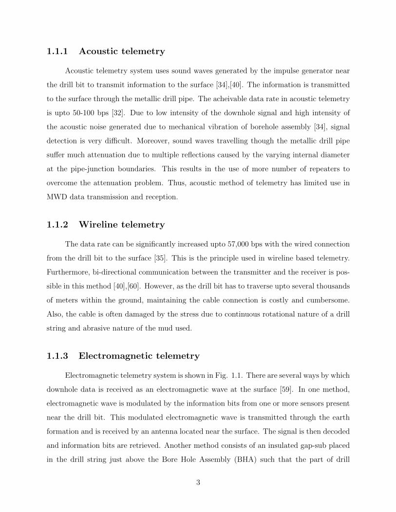
1.1.1 Acoustic telemetry

Acoustic telemetry system uses sound waves generated by the impulse generator near

the drill bit to transmit information to the surface [34],[40]. The information is transmitted

to the surface through the metallic drill pipe. The acheivable data rate in acoustic telemetry

is upto 50-100 bps [32]. Due to low intensity of the downhole signal and high intensity of

the acoustic noise generated due to mechanical vibration of borehole assembly [34], signal

detection is very difficult. Moreover, sound waves travelling though the metallic drill pipe

suffer much attenuation due to multiple reflections caused by the varying internal diameter

at the pipe-junction boundaries. This results in the use of more number of repeaters to

overcome the attenuation problem. Thus, acoustic method of telemetry has limited use in

MWD data transmission and reception.

1.1.2 Wireline telemetry

The data rate can be significantly increased upto 57,000 bps with the wired connection

from the drill bit to the surface [35]. This is the principle used in wireline based telemetry.

Furthermore, bi-directional communication between the transmitter and the receiver is pos-

sible in this method [40],[60]. However, as the drill bit has to traverse upto several thousands

of meters within the ground, maintaining the cable connection is costly and cumbersome.

Also, the cable is often damaged by the stress due to continuous rotational nature of a drill

string and abrasive nature of the mud used.

1.1.3 Electromagnetic telemetry

Electromagnetic telemetry system is shown in Fig. 1.1. There are several ways by which

downhole data is received as an electromagnetic wave at the surface [59]. In one method,

electromagnetic wave is modulated by the information bits from one or more sensors present

near the drill bit. This modulated electromagnetic wave is transmitted through the earth

formation and is received by an antenna located near the surface. The signal is then decoded

and information bits are retrieved. Another method consists of an insulated gap-sub placed

in the drill string just above the Bore Hole Assembly (BHA) such that the part of drill

3

string above and below the gap-sub act as two sides of an antenna. When an alternating

voltage modulated with information bits is applied across the two ends of an insulated gap-

sub, current is generated which propagates along the drill string. The surface transceiver

measures the voltage difference between the drilling rig and remote ground resulting from

this current, which is then decoded.

Electromagnetic based borehole telemetry has several advantages and limitations over

mud pulse telemetry (MPT). Some of the advantages include higher data rates, reliable

bi-directional communication between downhole and surface, higher resistance to the noise

resulting from moving downhole parts [41]. The data rate can be as high as 100 bps [33]

with the use of repeaters and signal quality is unaffected by the intermittent mud flow

unlike in mud pulse telemetry. Limitations include relatively low depth capability and data

communication is severely affected for particular type of formation containing high amount

of salt (due to increase in ground conductivity). The quality of the received signal measured

by the parameter Signal to Noise Ratio (SNR) is affected by the attenuation from the various

layers of earth acting as lossy dielectrics. One method to enhance the SNR is by increasing

the power of transmitted signal. This however, comes at an expense of high battery power

consumption, which is undesirable. As an alternative, adaptive noise cancellation circuitry

is used for increasing the SNR in electromagnetic based telemetry [60].

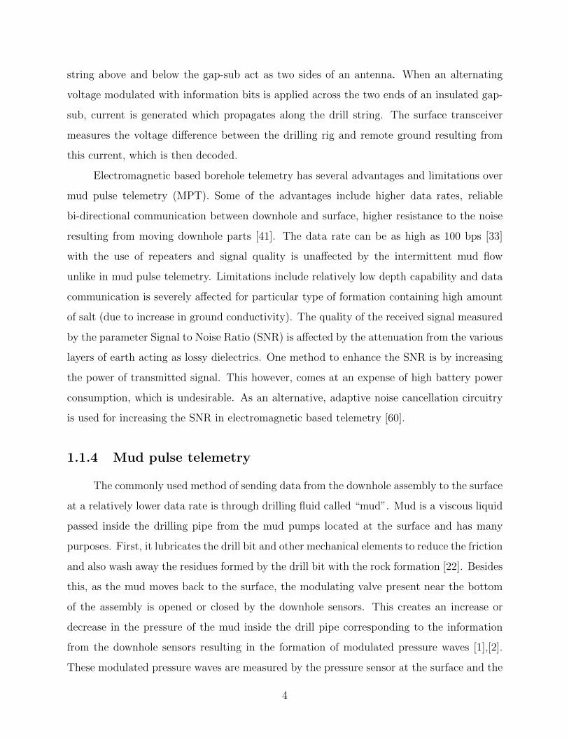
1.1.4 Mud pulse telemetry

The commonly used method of sending data from the downhole assembly to the surface

at a relatively lower data rate is through drilling fluid called “mud”. Mud is a viscous liquid

passed inside the drilling pipe from the mud pumps located at the surface and has many

purposes. First, it lubricates the drill bit and other mechanical elements to reduce the friction

and also wash away the residues formed by the drill bit with the rock formation [22]. Besides

this, as the mud moves back to the surface, the modulating valve present near the bottom

of the assembly is opened or closed by the downhole sensors. This creates an increase or

decrease in the pressure of the mud inside the drill pipe corresponding to the information

from the downhole sensors resulting in the formation of modulated pressure waves [1],[2].

These modulated pressure waves are measured by the pressure sensor at the surface and the

4

downhole data is decoded.

Pressure waves can be discrete pulses or continuous waves. The selection of the partic-

ular type depends on the feasibility and requirement of the rig operator. Discrete pulses are

high amplitude and low frequency pulses that are used in deep wells as it makes them easier

to detect readily at the surface. Continuous waves on the other hand are of lower amplitudes

[5]. By varying the frequency of a pulser, various modulation schemes such as Binary Phase

Shift keying (BPSK) and Quadrature Phase Shift Keying (QPSK) providing flexible data

rates can be achieved. Data rates from 20 to 40 bps are possible with continuous waves

[3],[5]. The other significant advantage of using the carrier modulation is that the receiver

may employ coherent detection method to achieve same bit error rate as in demodulation of

discrete pressure pulses at a lower signal to noise ratio. Their limitation however includes

lower SNR due to their low amplitudes and thus, it is hard to detect small amplitude con-

tinuous waves from deep wells even at low frequencies. The generation mechanism of both

discrete and continuous pressure waves are discussed in detail in Chapter 2.

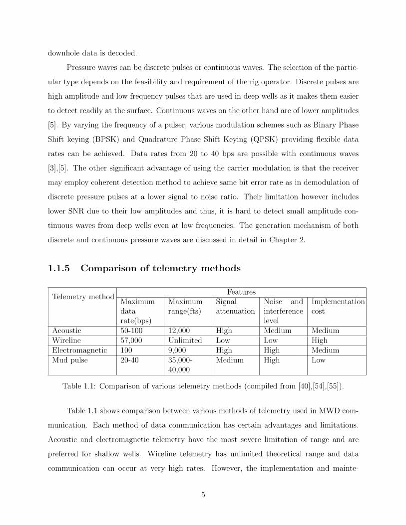
1.1.5 Comparison of telemetry methods

Telemetry methodFeatures

Maximumdatarate(bps)

Maximumrange(fts)

Signalattenuation

Noise andinterferencelevel

Implementationcost

Acoustic 50-100 12,000 High Medium MediumWireline 57,000 Unlimited Low Low HighElectromagnetic 100 9,000 High High MediumMud pulse 20-40 35,000-

40,000Medium High Low

Table 1.1: Comparison of various telemetry methods (compiled from [40],[54],[55]).

Table 1.1 shows comparison between various methods of telemetry used in MWD com-

munication. Each method of data communication has certain advantages and limitations.

Acoustic and electromagnetic telemetry have the most severe limitation of range and are

preferred for shallow wells. Wireline telemetry has unlimited theoretical range and data

communication can occur at very high rates. However, the implementation and mainte-

5

nance cost is very high as it often suffers from cable breakage due to the rotatory nature of

a drill string. Although mud pulse telemetry has the lowest data rate, it is suited for deep

well with minimum cost. This makes mud pulse telemetry a widely used method of MWD.

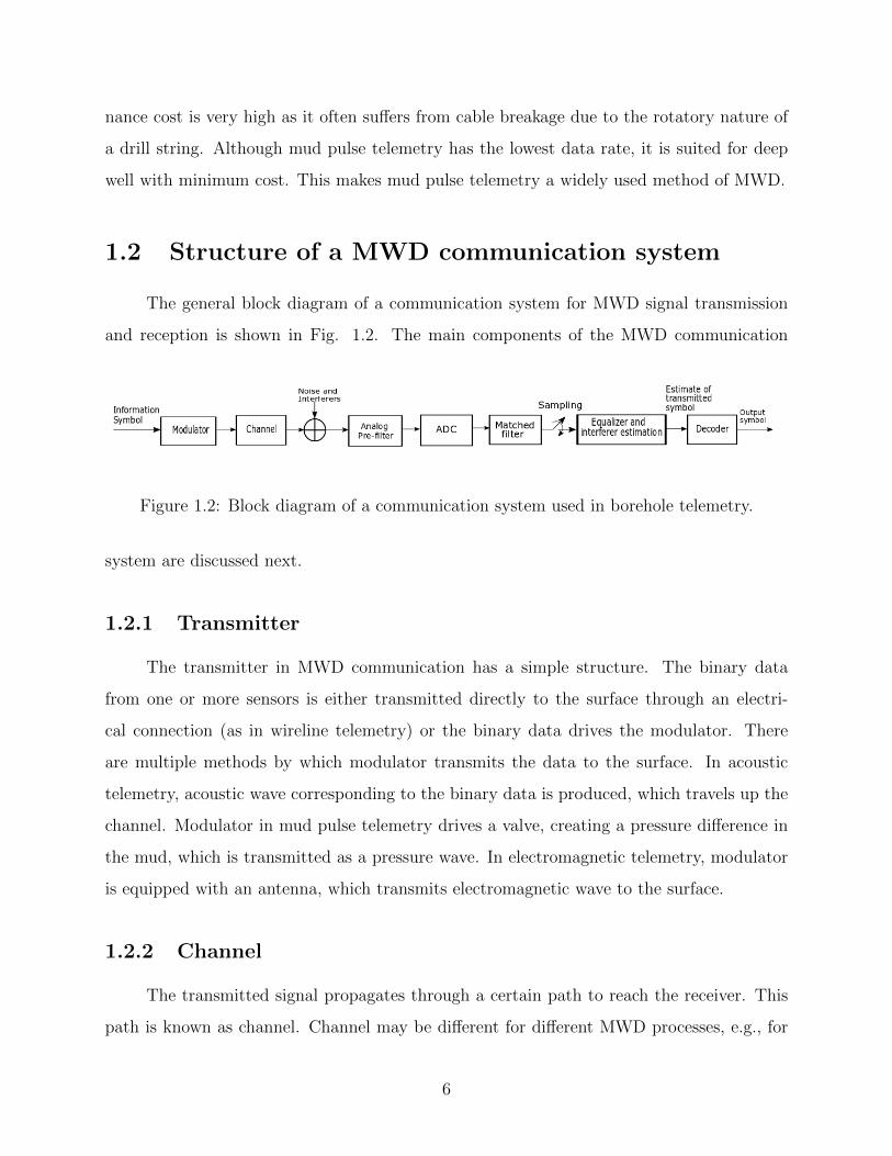
1.2 Structure of a MWD communication system

The general block diagram of a communication system for MWD signal transmission

and reception is shown in Fig. 1.2. The main components of the MWD communication

Figure 1.2: Block diagram of a communication system used in borehole telemetry.

system are discussed next.

1.2.1 Transmitter

The transmitter in MWD communication has a simple structure. The binary data

from one or more sensors is either transmitted directly to the surface through an electri-

cal connection (as in wireline telemetry) or the binary data drives the modulator. There

are multiple methods by which modulator transmits the data to the surface. In acoustic

telemetry, acoustic wave corresponding to the binary data is produced, which travels up the

channel. Modulator in mud pulse telemetry drives a valve, creating a pressure difference in

the mud, which is transmitted as a pressure wave. In electromagnetic telemetry, modulator

is equipped with an antenna, which transmits electromagnetic wave to the surface.

1.2.2 Channel

The transmitted signal propagates through a certain path to reach the receiver. This

path is known as channel. Channel may be different for different MWD processes, e.g., for

6

mud pulse telemetry, mud acts as a channel while for electromagnetic borehole telemetry,

earth acts as a channel. The signal propagating through the channel suffers multiple re-

flections and refractions at various boundaries. This leads to smearing of a symbol over the

period of an adjacent symbol, the phenomenon commonly known as intersymbol interference

(ISI). ISI causes erroneous detection of bits at the receiver.

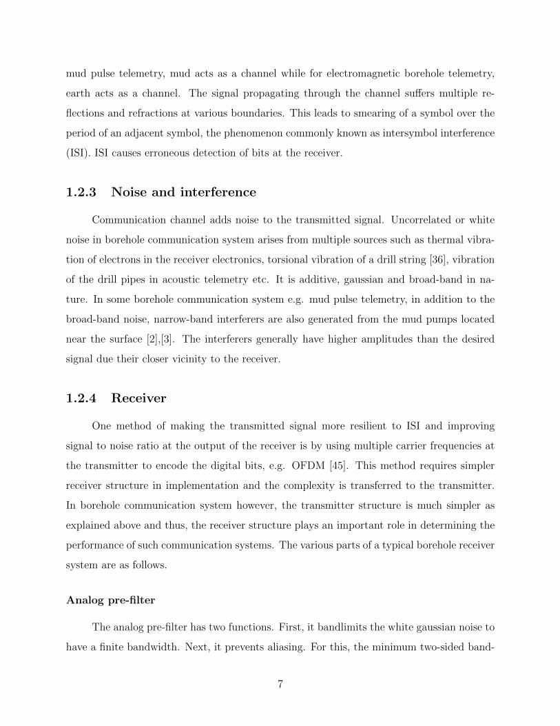
1.2.3 Noise and interference

Communication channel adds noise to the transmitted signal. Uncorrelated or white

noise in borehole communication system arises from multiple sources such as thermal vibra-

tion of electrons in the receiver electronics, torsional vibration of a drill string [36], vibration

of the drill pipes in acoustic telemetry etc. It is additive, gaussian and broad-band in na-

ture. In some borehole communication system e.g. mud pulse telemetry, in addition to the

broad-band noise, narrow-band interferers are also generated from the mud pumps located

near the surface [2],[3]. The interferers generally have higher amplitudes than the desired

signal due their closer vicinity to the receiver.

1.2.4 Receiver

One method of making the transmitted signal more resilient to ISI and improving

signal to noise ratio at the output of the receiver is by using multiple carrier frequencies at

the transmitter to encode the digital bits, e.g. OFDM [45]. This method requires simpler

receiver structure in implementation and the complexity is transferred to the transmitter.

In borehole communication system however, the transmitter structure is much simpler as

explained above and thus, the receiver structure plays an important role in determining the

performance of such communication systems. The various parts of a typical borehole receiver

system are as follows.

Analog pre-filter

The analog pre-filter has two functions. First, it bandlimits the white gaussian noise to

have a finite bandwidth. Next, it prevents aliasing. For this, the minimum two-sided band-

7

width of an analog pre-filter is assumed to be equal to the sampling frequency. Therefore, it

is also known as an anti-aliasing filter.

ADC and matched filter

The analog waveform is sampled and digitized for further processing. For a known chan-

nel, a matched filter is matched to the overall impulse response of channel and pulse shaping

filter. Such matched filter maximizes the SNR, therefore, the receiver performance becomes

optimum. However, for unknown channels, the matched filter may be simply matched to the

pulse shaping filter. In such case the receiver performance is sub-optimum. The output of a

matched filter is sampled either every symbol period or some integral multiples of a symbol

period. These samples act as the input to an equalizer.

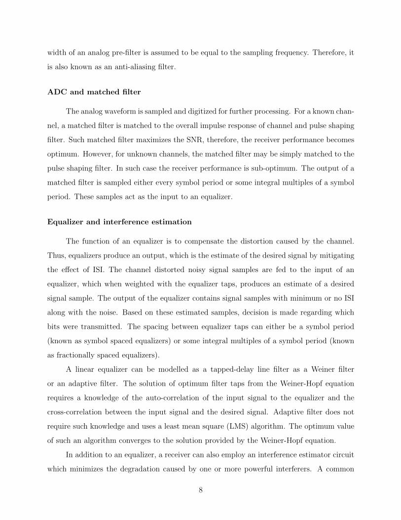
Equalizer and interference estimation

The function of an equalizer is to compensate the distortion caused by the channel.

Thus, equalizers produce an output, which is the estimate of the desired signal by mitigating

the effect of ISI. The channel distorted noisy signal samples are fed to the input of an

equalizer, which when weighted with the equalizer taps, produces an estimate of a desired

signal sample. The output of the equalizer contains signal samples with minimum or no ISI

along with the noise. Based on these estimated samples, decision is made regarding which

bits were transmitted. The spacing between equalizer taps can either be a symbol period

(known as symbol spaced equalizers) or some integral multiples of a symbol period (known

as fractionally spaced equalizers).

A linear equalizer can be modelled as a tapped-delay line filter as a Weiner filter

or an adaptive filter. The solution of optimum filter taps from the Weiner-Hopf equation

requires a knowledge of the auto-correlation of the input signal to the equalizer and the

cross-correlation between the input signal and the desired signal. Adaptive filter does not

require such knowledge and uses a least mean square (LMS) algorithm. The optimum value

of such an algorithm converges to the solution provided by the Weiner-Hopf equation.

In addition to an equalizer, a receiver can also employ an interference estimator circuit

which minimizes the degradation caused by one or more powerful interferers. A common

8

method used by such circuits often includes frequency transforming the received signal and

separating the interferers from the signal.

Decoder

Decoder is a decision making device. It compares the output estimates from an equal-

izer with a known threshold and decides which of the transmitted symbol was sent by the

transmitter.

With the general introduction of various methods and communication system used in

the borehole telemetry methods, now this thesis focusses on mud pulse telemetry system as

it is the most widely used method of transmitting and receiving the downhole signal to the

surface.

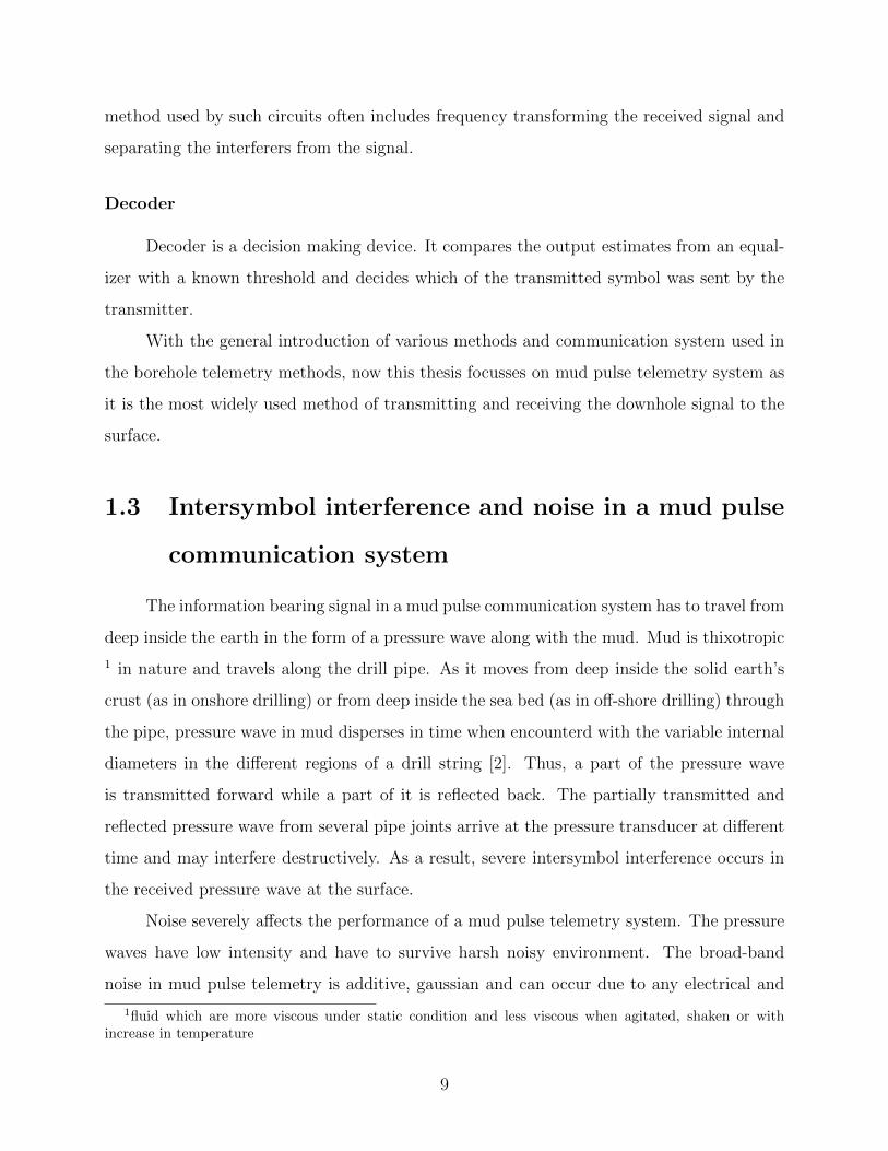
1.3 Intersymbol interference and noise in a mud pulse

communication system

The information bearing signal in a mud pulse communication system has to travel from

deep inside the earth in the form of a pressure wave along with the mud. Mud is thixotropic

1 in nature and travels along the drill pipe. As it moves from deep inside the solid earth’s

crust (as in onshore drilling) or from deep inside the sea bed (as in off-shore drilling) through

the pipe, pressure wave in mud disperses in time when encounterd with the variable internal

diameters in the different regions of a drill string [2]. Thus, a part of the pressure wave

is transmitted forward while a part of it is reflected back. The partially transmitted and

reflected pressure wave from several pipe joints arrive at the pressure transducer at different

time and may interfere destructively. As a result, severe intersymbol interference occurs in

the received pressure wave at the surface.

Noise severely affects the performance of a mud pulse telemetry system. The pressure

waves have low intensity and have to survive harsh noisy environment. The broad-band

noise in mud pulse telemetry is additive, gaussian and can occur due to any electrical and

1fluid which are more viscous under static condition and less viscous when agitated, shaken or withincrease in temperature

9

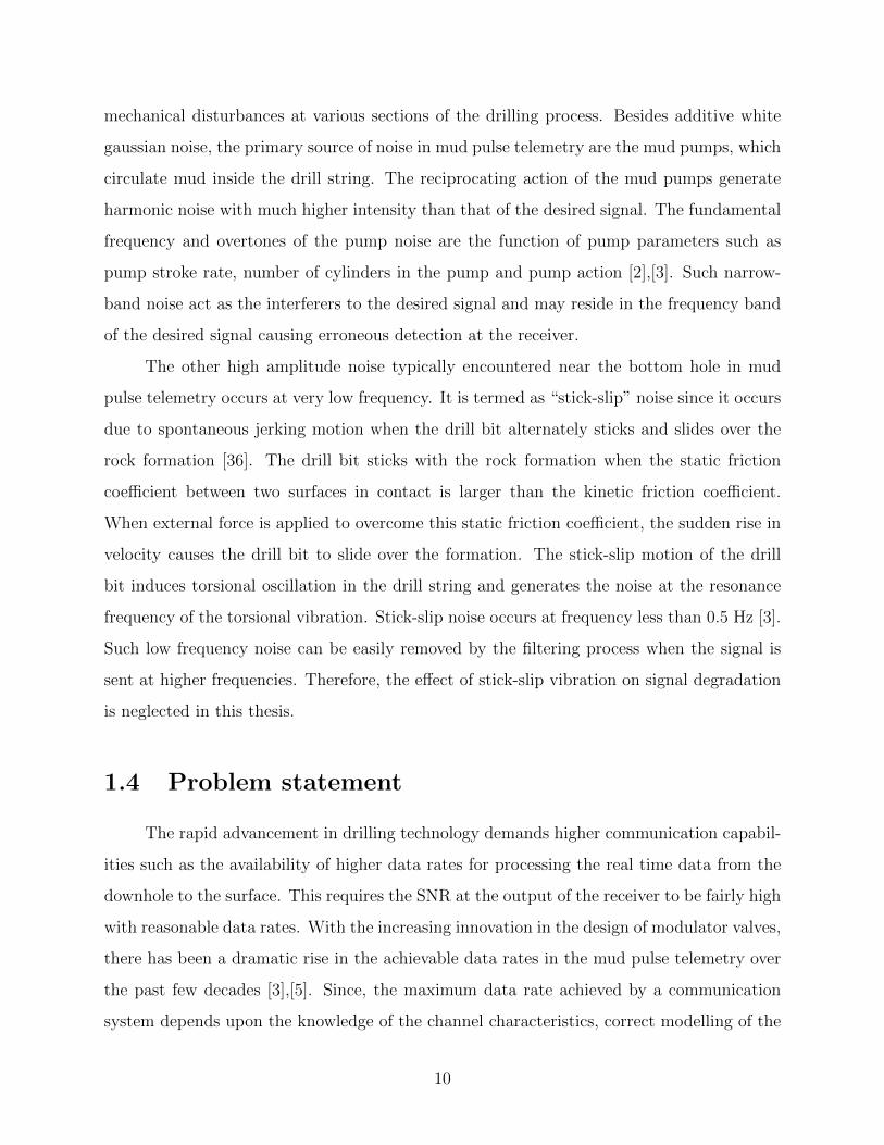
mechanical disturbances at various sections of the drilling process. Besides additive white

gaussian noise, the primary source of noise in mud pulse telemetry are the mud pumps, which

circulate mud inside the drill string. The reciprocating action of the mud pumps generate

harmonic noise with much higher intensity than that of the desired signal. The fundamental

frequency and overtones of the pump noise are the function of pump parameters such as

pump stroke rate, number of cylinders in the pump and pump action [2],[3]. Such narrow-

band noise act as the interferers to the desired signal and may reside in the frequency band

of the desired signal causing erroneous detection at the receiver.

The other high amplitude noise typically encountered near the bottom hole in mud

pulse telemetry occurs at very low frequency. It is termed as “stick-slip” noise since it occurs

due to spontaneous jerking motion when the drill bit alternately sticks and slides over the

rock formation [36]. The drill bit sticks with the rock formation when the static friction

coefficient between two surfaces in contact is larger than the kinetic friction coefficient.

When external force is applied to overcome this static friction coefficient, the sudden rise in

velocity causes the drill bit to slide over the formation. The stick-slip motion of the drill

bit induces torsional oscillation in the drill string and generates the noise at the resonance

frequency of the torsional vibration. Stick-slip noise occurs at frequency less than 0.5 Hz [3].

Such low frequency noise can be easily removed by the filtering process when the signal is

sent at higher frequencies. Therefore, the effect of stick-slip vibration on signal degradation

is neglected in this thesis.

1.4 Problem statement

The rapid advancement in drilling technology demands higher communication capabil-

ities such as the availability of higher data rates for processing the real time data from the

downhole to the surface. This requires the SNR at the output of the receiver to be fairly high

with reasonable data rates. With the increasing innovation in the design of modulator valves,

there has been a dramatic rise in the achievable data rates in the mud pulse telemetry over

the past few decades [3],[5]. Since, the maximum data rate achieved by a communication

system depends upon the knowledge of the channel characteristics, correct modelling of the

10

mud channel plays an important role in improving the data rate of the mud pulse telemetry

system.

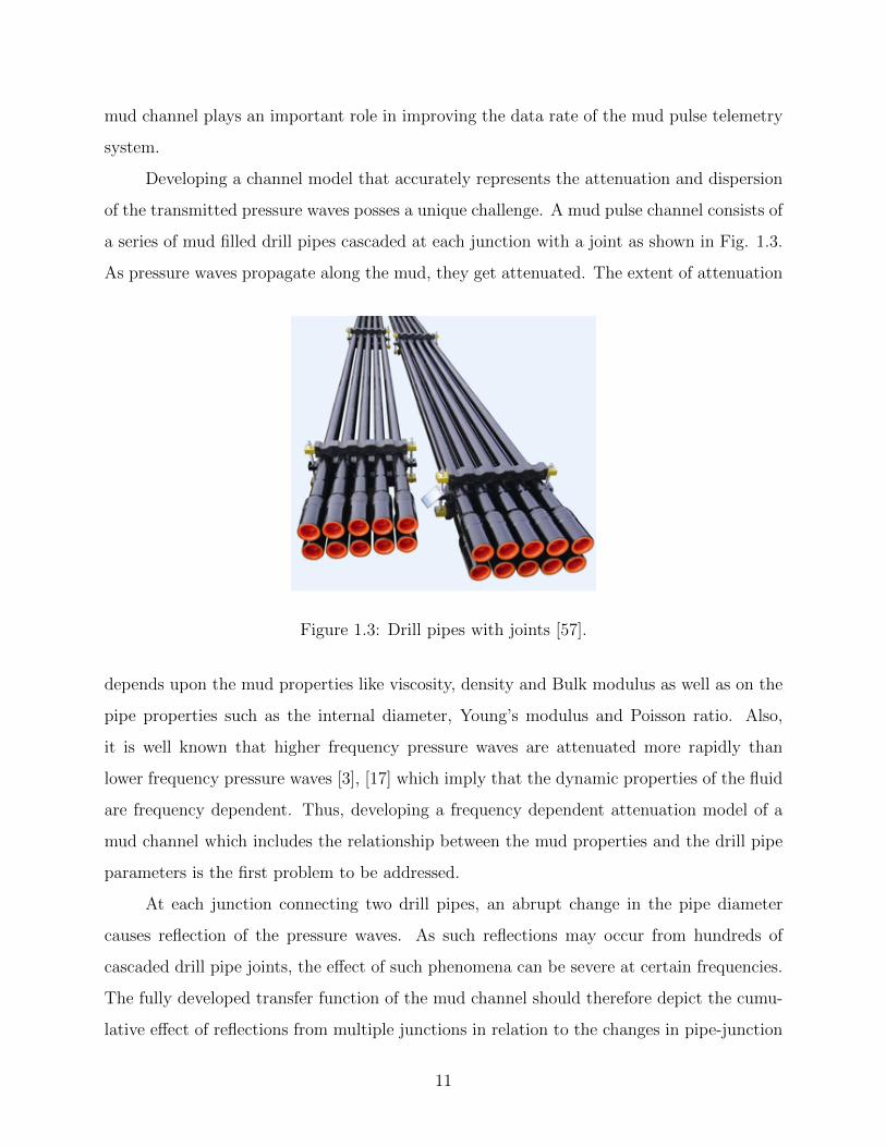
Developing a channel model that accurately represents the attenuation and dispersion

of the transmitted pressure waves posses a unique challenge. A mud pulse channel consists of

a series of mud filled drill pipes cascaded at each junction with a joint as shown in Fig. 1.3.

As pressure waves propagate along the mud, they get attenuated. The extent of attenuation

Figure 1.3: Drill pipes with joints [57].

depends upon the mud properties like viscosity, density and Bulk modulus as well as on the

pipe properties such as the internal diameter, Young’s modulus and Poisson ratio. Also,

it is well known that higher frequency pressure waves are attenuated more rapidly than

lower frequency pressure waves [3], [17] which imply that the dynamic properties of the fluid

are frequency dependent. Thus, developing a frequency dependent attenuation model of a

mud channel which includes the relationship between the mud properties and the drill pipe

parameters is the first problem to be addressed.

At each junction connecting two drill pipes, an abrupt change in the pipe diameter

causes reflection of the pressure waves. As such reflections may occur from hundreds of

cascaded drill pipe joints, the effect of such phenomena can be severe at certain frequencies.

The fully developed transfer function of the mud channel should therefore depict the cumu-

lative effect of reflections from multiple junctions in relation to the changes in pipe-junction

11

diameters which is the second problem to be resolved.

The primary noise from the mud pump consists of multiple narrow-band sinusoidal

interferers. One existing method commonly used to avoid the effect of pump noise is to

transmit signal in the region of spectrum containing minimum noise. This method how-

ever, cannot remove all the narrow-band pump noise when multiple harmonics of significant

amplitudes are present in the signal frequency band. Furthermore, this method imposes a

restriction in the range of signal frequency selection which is undesirable. Thus, in order

to have more flexibility in selecting the range of signal frequency, a suitable filter capable

of selectively cancelling out narrow-band interferers present in the signal frequency band is

desired which is the next issue to be addressed.

Once the mud channel is modelled, it is required to design a model of a receiver by

compensating the effect of mud channel distortion with an equalizer. Further, the perfor-

mance improvement of the receiver system after cancelling out the interferers and mitigating

the channel effects needs to be studied by evaluating performance metrics such as bit error

rate (BER). Quantifying the performance of a mud pulse receiver can be very essential for

drill rig operators to monitor and evaluate the performance of mud pulse communication

system, which is the final problem to be addressed by this thesis.

1.5 Literature review

The concept of sending encoded data from downhole electronics as a pressure wave has

been widely studied in the past few decades. The early work of using discrete mud pulses

to send modulated pressure waves to the surface from the downhole was described by Arps

and Arps in [1] in which a mud pulse communication system prototype was designed and

field tested. The modulator consisted of a Plunger valve in the drill collar controlled by

the downhole sensors thus generating positive pressure pulses. The data rate achieved was

less than 1 bps. More advanced type of phase modulated continuous waves using rotary

valve controlled by servomotors were discussed in the work done by Patton et al. [2]. The

maximum data rate achieved was 3 bps. The data rates in continuous wave telemetry

has since been significantly improved by the innovation in the design of the rotor-stator

12

arrangement and the motion of the rotor. Hutin et al. [3] have described a mud-siren

consisting of continuously moving rotor capable of generating a carrier modulated wave at

24 Hz. A novel pulser capable of generating both base-band and carrier modulated wave

was described in [4] and [5]. This novel pulser uses a sheer valve comprising of stator and

oscillating rotor. By exploiting the fact that rotor velocity reaches zero at the end of each

oscillation period, the frequency can be changed instantaneously at these periods without

physically accelerating or decelerating the rotor disc, thus saving the time interval for this

transition as in mud-siren. The maximum data rate of 40 bps has been achieved with this

sheer valve modulator and shows a possibility of further increasing data rates in future.

Further details about the continuous wave mud pulser is available in U.S. patents [6], [7] and

[8]. Although all aforementioned works focus on improving the data rate, no efforts have

been made to understand and characterise the channel through which mud pulse propagates.

The close analogy between the nature of hydraulic and electrical system suggests that

the parameters used to describe the dynamic behaviour of an electrical system can be used

with their equivalent counterparts in hydraulic system to describe the dynamic behaviour

of a fluid system. The basic elements such as resistance, inductance and capacitance that

are used to describe the voltage-current relation in a distributed electrical circuit can also

be used to describe the pressure-flow rate relation in a fluid system [9]. Thus, by comparing

the fluid system model with the standard transmission line model, the analysis of a complex

fluid line can be easily made. This fact is exploited in the pioneering work by Auslander [10].

With a linear mechanical system modelled as an equivalent transmission line, the pressure

and flow rate relationship at the two ends of a pipe has been described. Furthermore, by

decomposing the pressure and flow rate into equivalent wave components travelling in both

directions of a pipe, the scattering matrix of a junction between pipes has been developed

describing the effect of wave reflection and transmission at the boundary of a pipe. Boucher

et al. [11] and Beck et al. [12] adapted this theory of the fluid transmission line to further

explain the pneumatic and viscous liquid flow in a conduit. The model were experimentally

verified and resulted in a good agreement with the theoretical model described. Although

these researches provide a useful insight for the application of a fluid transmission line theory

to describe the mud propagation through a drill string in a mud pulse telemetry, these works

13

however describe the fluid transmission line as a pure time delay circuit assuming linear

resistance at the junction alone, with the resistance at the pipe being neglected. Authors in

[13] and [14] considered viscous resistance as a frequency dependent parameter and derived

the frequency response of pneumatic flow in a closed pipe. Further equations and solutions of

forced oscillatory flow in a pipeline system and frequency response analysis of a fluid system

developed from the fluid transmission line model have been described in [15].

Desbrandes et al. [17], [18] have theoretically and experimentally studied the mud pulse

propagation and attenuation characteristics of the mud channel. Various factors affecting

the mud pulse attenuation have been described. Their model is extensively used to study the

mud pulse propagation in mud pulse telemetry applications. However, their study cannot

fully describe the realistic mud pulse propagation as the described channel is over simplified

and cannot account for the reflection of the pressure wave at multiple pipe joints.

Hutin et al. [3] have adopted the mud channel characteristics developed by [17], [18].

Of the most significance, they have expressed the mud pump noise as a function of pump

parameters. Albeit, the authors suggest a method of pump noise removal by transmitting the

signal in the region of spectrum containing no noise, this method of noise removal does not

always work for the imperfect mud pumps where harmonics have dominant magnitudes com-

pared to the fundamental frequency and thus may reside in the spectrum of signal. Another

method of mud pump noise cancellation is rather manual and requires much computation as

described in U.S. patent [19]. In their method, mud pressure is calibrated as a function of

pump piston position. When the MWD signal is transmitted, the piston position is tracked

and the pump noise is subtracted using the calibration information.

Pioneering work in adaptive filtering of noise signal includes the work of Widrow and

Hoff [20]. It describes the equalization of channel distorted signal using steepest descent

gradient with a LMS algorithm. This method of signal processing has been borrowed and

implemented in mud pulse signal processing as well. For example, U.S patent [21] describes

the adaptive filtering of pump noise using LMS algorithm. In this method, the frequency

of at least one mud pump is determined and the noise corresponding to this frequency is

represented as a harmonic series. The noise is then cancelled out using LMS algorithm.

Authors in [22] have roughly approximated the mud communication channel as a low pass

14

RC filter with a cut-off frequency of 0.02 Hz and a DC offset of 2000 psi. In their work,

a complex fractionally spaced decision feedback equalizer was used to counter the effect of

intersymbol interference. The cut-off frequency approximation of a mud channel with a low

pass filter, however needs to be justified for real time mud pulse propagation through the

mud channel. The methods of pump noise removal and mud channel equalization imply the

increasing use of signal processing techniques from cellular communication to the mud pulse

telemetry. Thus, once the mud channel is developed, the distortion caused by the channel

can be compensated by using the suitable type of equalizers.

The concept of an adaptive LMS filter has been modified and implemented to either

enhance or suppress the narrow-band signals in a broad-band noise for cellular systems. For

example, Zeidler et al. in [23] discussed the enhancement of multiple sinusoidal components

in a white noise. By a suitable delay of the input signal, the LMS filter was adapted to

generate the transfer function of the useful narrow-band sinusoids. Further modification

of LMS algorithm to suppress the narrow-band interferers in a wide-band spread spectrum

signal was shown by authors in [24] and [25]. In their work, the adaptive filter was adapted

to produce notches in the frequency band of narrow-band interferers, thus suppressing them.

Significant improvement in the output signal to noise and interference ratio (SINR) has been

reported. These works, however, aim to enhance the capability of a receiver designed for

cellular communication system. As the mud pulse telemetry system differs in the propagation

channel and the noise that affect the pressure waves, a careful analysis of the mud channel

and distribution of the noise and interferers need to be done before these concepts can be

implemented in the mud pulse telemetry system.

1.6 Contribution of this research

The first contribution of this thesis is the mathematical characterization of the mud

channel. The modelled mud channel accounts for the signal distortion due to the attenua-

tion and dispersion of the pressure waves at multiple junctions in a drill string through the

implementation of a fluid transmission line model. The attenuation characteristics of the

propagating mud developed through the fluid transmission line model at different frequen-

15

cies is shown to closely agree with the experimentally determined attenuation characteristics

of the mud channel described in [17] and [18]. The transfer function of the mud channel

has been analytically derived from the fluid transmission line model and is verified with the

transfer function of an equivalent electrical transmission line model in the Keysight’s Ad-

vanced Design System (ADS). The effect of reflections from the multiple junctions on channel

transfer function has been described. It has been shown that the location of standpipe trans-

ducer from the mud pump affects the frequency response nature of the mud channel. Thus,

once the nature of frequency response of a mud channel is determined, it is possible to de-

sign efficient receivers with improved bit error rate. With the increasing innovation towards

higher data rates in mud pulse telemetry, such realistic mud pulse channel model helps in

the efficient utilization of the channel bandwidth.

Another contribution of this thesis is the implementation of the concept of cancelling

out the narrow-band interferers present in a wide-band signal as described in [24] and [25]

in mud pulse telemetry to reject the narrow-band interferers from the mud pump. This

method of cancelling out the narrow-band interferers in mud pulse telemetry has significant

advantages due to the fact that interferers present in the signal spectrum can be adaptively

removed without having to transmit the signal in the region of no pump noise. By trans-

mitting mud pulses at a higher rate and sufficiently delaying the received signal so that the

signal samples on adjacent taps are least correlated as compared to more correlated interferer

samples, multiple interferers are removed creating notches in the signal spectrum. Although

the formation of notches introduces some distortion in the desired signal, the degradation

due to such notches is repaired easily with the use of an equalizer. It has been shown that

such a notch filter enhances the SINR as the power of an interferer increases. As the mud

pump interferers have higher power compared to the signal, the usefulness of such a notch

filter is further apparent.

The final contribution of this thesis is the compensation of the distortion caused by

the mud channel and study the receiver performance. The receiver performance is compared

for different data rates and interference powers. Equalization is based on the Weiner-Hopf

filter modelled as a tapped delay-line filter. The performance metric used to evaluate the

performance of the equalizer and notch filter is the bit error rate. It has been shown that

16

significant improvement in the bit error rate can be achieved with the use of an equalizer

and notch filter in a mud pulse receiver. It has also been shown that the use of a notch filter

to cancel out narrow-band interferers and an equalizer to compensate the channel distortion

leads to the significant gain of drill depth, thus making higher data rates possible at greater

depths.

The results are significant as they accurately replicate the real time mud pulse prop-

agation, channel distortion and noise experienced by the mud pulse telemetry system. The

compensation of distortion caused by the channel combined with the interference cancella-

tion techniques considerably saves much of the valuable rig time operation while providing

the higher performance at fairly reasonable rates.

1.7 Organization of the thesis

This thesis contains six chapters. Chapter 2 describes the mud pulse communication

system in detail. It starts with an overview of the mud pulse communication system block

diagram and presents a trend of data rate improvement in the existing mud pulse telemetry.

Two types of mud pulse modulators commonly used in commercial applications to generate

continuous waves at higher data rates are described. An overview of a mud channel and two

different types of noise commonly encountered in the mud channel are presented. A brief

description of a stand pipe transducer used to receive the mud pulse signals is given.

Chapter 3 presents a detailed model of the mud channel developed from the fluid

transmission line theory. It begins with an elementary concept of the fluid transmission line

and describes the cascaded drill pipe system as an equivalent to the cascaded transmission

line structure. General solution of the pressure-flow rate relationships at the various regions

of a drill pipe is provided along with the attenuation characteristics of the mud flowing

through such cascaded pipes. Transfer function of a mud channel is then developed and the

impact of the transducer location on the frequency response of a mud channel is highlighted.

Chapter 4 provides a detailed description of the receiver design and its performance

analysis in a mud pulse telemetry system. After presenting the receiver structure used for

the optimum detection of pressure waves, BER degradation from the interferers is analysed

17

along with the removal of such interferers with the notch filter. Finally, the method of

compensating the channel distortion with the Weiner filter and LMS algorithm is briefed.

Chapter 5 presents results of simulations to support the theory developed in the pre-

ceding chapters and important implications from the simulation results are described.

Chapter 6 concludes the work. The significance and limitations of the work are de-

scribed and the potential future research is presented.

The final section of the thesis contains references and appendices on the fluid trans-

mission line analysis in terms of forward and reverse travelling wave variables. A scattering

matrix from the wave variables is derived for the potential future research. ADS simulation

of the transmission line as an equivalent to the fluid transmission line is also included in the

appendix.

18

Chapter 2

Mud pulse communication system

review

This chapter provides a general description of the structure of a mud pulse telemetry

system. Section 2.1 begins with an overview of the various parts of a mud pulse telemetry

system. In Section 2.2, a comparative study of the trend of data rate improvement in the mud

pulse telemetry is given. Section 2.3 describes a mud-pulse transmitter. As innovations in

the design of modulator valve have made it possible to achieve flexible data rates over recent

years, commonly used modulators to generate discrete pulses or continuous waves have been

described. Section 2.4 provides an insight into the communication channel through which

pressure waves travel to reach the receiver. It also describes the attenuation and reflection

phenomenon, which are the fundamental properties of a mud channel. The channel also

adds noise to the system. The source and nature of two commonly encountered noise in mud

pulse telemetry are given in Section 2.5. Section 2.6 concludes with an introduction of the

pressure sensor commonly known as standpipe transducer used to receive the pressure waves

near the surface.

2.1 Overview of a mud pulse telemetry system

A typical mud pulse telemetry system is shown in Fig. 2.1. The overall system com-

ponents fall under two regions: sub-surface region and surface region. Sub-surface region

19

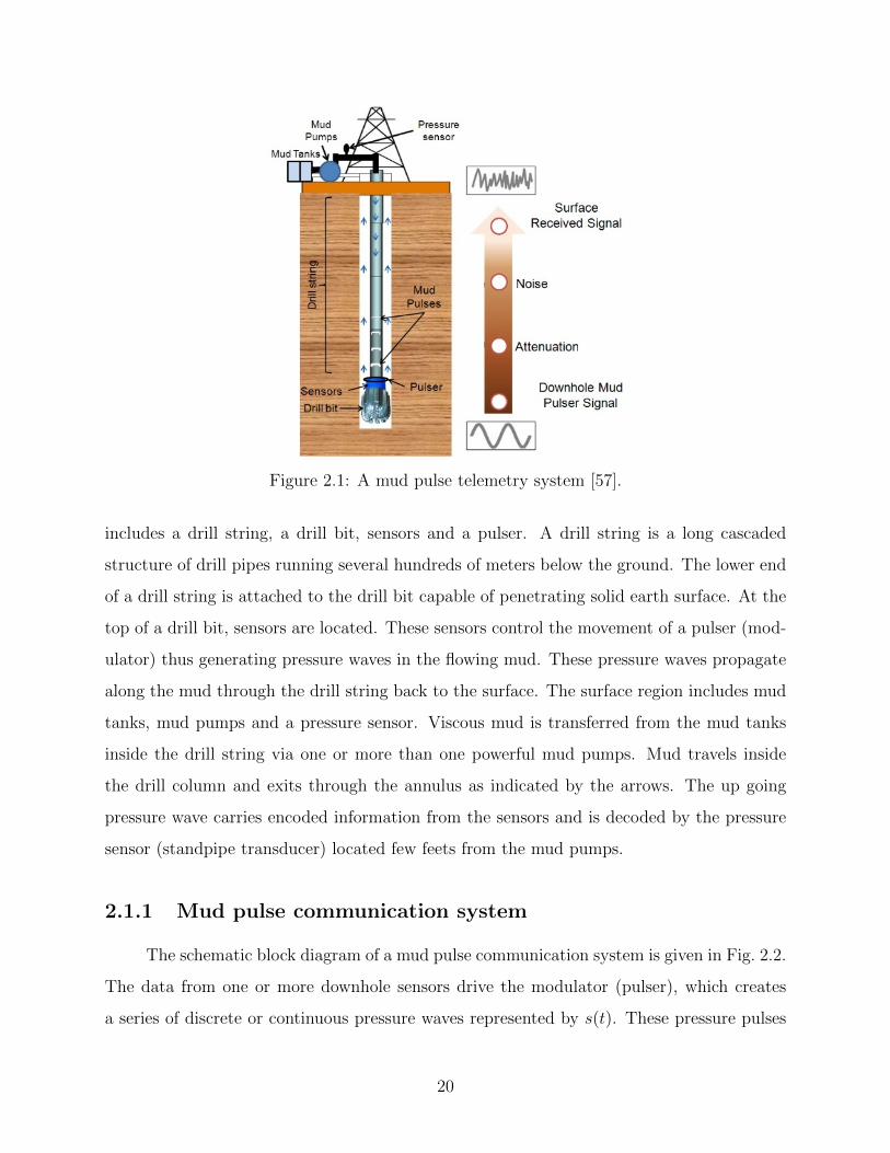
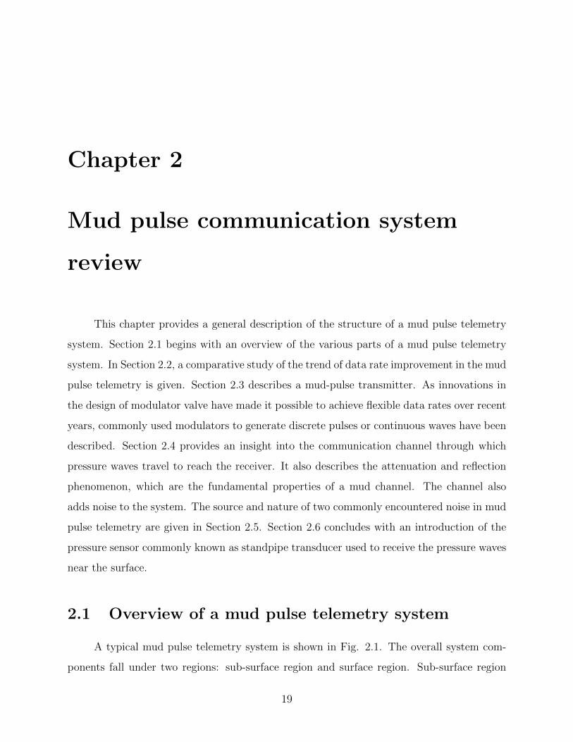
Figure 2.1: A mud pulse telemetry system [57].

includes a drill string, a drill bit, sensors and a pulser. A drill string is a long cascaded

structure of drill pipes running several hundreds of meters below the ground. The lower end

of a drill string is attached to the drill bit capable of penetrating solid earth surface. At the

top of a drill bit, sensors are located. These sensors control the movement of a pulser (mod-

ulator) thus generating pressure waves in the flowing mud. These pressure waves propagate

along the mud through the drill string back to the surface. The surface region includes mud

tanks, mud pumps and a pressure sensor. Viscous mud is transferred from the mud tanks

inside the drill string via one or more than one powerful mud pumps. Mud travels inside

the drill column and exits through the annulus as indicated by the arrows. The up going

pressure wave carries encoded information from the sensors and is decoded by the pressure

sensor (standpipe transducer) located few feets from the mud pumps.

2.1.1 Mud pulse communication system

The schematic block diagram of a mud pulse communication system is given in Fig. 2.2.

The data from one or more downhole sensors drive the modulator (pulser), which creates

a series of discrete or continuous pressure waves represented by s(t). These pressure pulses

20

Sensor data

Modulator(pulser)

Mud Channel

Mud pump interferers

White gaussian noise n(t) and

standpipe transducer (pressure sensor)

Signal processing circuit

Decision device

Output datas(t)

hc(t)

i(t)

r(t)x(t)In

Figure 2.2: Block diagram of a mud pulse communication system.

propagate through the mud channel. The output pressure waves of the channel can be

represented as

x(t) =

∞∫−∞

s(τ)hc(t− τ)dτ, (2.1)

where hc(t) represents the impulse response of the mud channel.

As pressure waves reach to the surface, they get corrupted by wideband additive gaussian

noise n(t) and interfering signals from the mud pumps i(t). Thus, the received signal at the

standpipe transducer is given as

r(t) = x(t) + n(t) + i(t). (2.2)

The corrupted signal received by the standpipe transducer is then subjected to the

signal processing circuit where the received signal is sampled, filtered to remove mud pump

interferers and equalized to compensate the channel distortion. The receiver then makes

decision to predict the transmitted data from the sensor.

2.2 Data rates in mud pulse telemetry

In mud pulse telemetry system, the data collected from the downhole fall under two

categories: Measurement While Drilling (MWD) data and Logging While Drilling (LWD)

data. MWD data contain information for evaluating the trajectory of wellbore. Data include

azimuth and inclination of the drill bit so that the rig operator knows the direction in which

the well is being bored and the drill bit is moving. MWD data are sent to the surface in real

time as pressure waves. LWD refer to the geological data stored in the memory of various

sensors below the ground. Some of these data include information of downhole annular

pressure, temperature, resistivity, density, porosity, nature of hydrocarbon etc. These stored

21

data are either downloaded and accessed when the tools are pulled back to the surface or

transmitted in the real time to the surface in a similar way as MWD data via pressure waves.

As rig day rates 1 continue to increase, the necessity of more data to analyse the

downhole conditions while the actual drilling operation takes place, is sure to increase as

well. The elegant and economic solution of this problem is to increase the data rate of the

mud pulse telemetry system. In fact, over the past few years, fair amount of efforts have

been put in by several companies in the design of mud pulse transmitters to achieve higher

data rates. As an example, Fig. 2.3 depicts the improvement in the data rates between 2000

and 2007. For a comparison, the data rate of mud pulse telemetry systems in 2000 was in

the range of 1 bps while in 2007 it was nearly 40 bps for shallow wells. The graph also shows

the variation of the data rate with the increase in the depth of the borehole. Clearly, as data

rate increases, the signal propagation depth decreases. This is due to the fact that higher

frequencies attenuate rapidly than lower frequencies as the depth increases.

Figure 2.3: Comparison of data rates of mud pulse telemetry systems between 2000-2007with depth [5].

Although Fig. 2.3 shows increment in the data rates over past few years, still, the

achieved data rate so far seems to be quite low. One of the main reason behind such low

data rates is the inability of the existing works to characterize the behaviour of the pressure

1cost of renting a drilling rig per day

22

waves through the mud channel as the capacity of any communication system depends on

the knowledge of the channel characteristics. Therefore, it is very important to characterize

the mud channel in order to design high performance receivers for the mud pulse telemetry

systems.

2.3 Mud pulse transmitter

A mud pulse transmitter is an assembly of a valve controlled modulator/pulser used

to create a pressure difference in the flowing mud. As shown in Fig. 2.1, to generate the

pressure waves, downhole digital data from the sensors trigger the mechanical motor present

in the borehole assembly. By controlling the valve action via motion of the motor, change in

pressure in the flowing mud is achieved. This change in pressure propagates up along the mud

and is detected by the pressure sensor. Early telemetry systems generated discrete pressure

pulses. These discrete pulses are still used by some of the rig operators due to their ease of

generation and reliability in deeper wells. With the introduction of rotor-stator arrangement

in the motor, continuous pressure waves are generated. This arrangement of the rotor and

stator has seen significant increase in achievable data rates. Also, by increasing or decreasing

the speed of the rotor, carrier modulation is possible. Both discrete and continuous signals

generating modulators are discussed below.

2.3.1 Discrete Pulser

A discrete pulser generates binary pressure waveform in the flowing mud. Increase in

pressure corresponds to “1” whereas decrease in pressure corresponds to“0”. Discrete pulses

of very high amplitudes can be easily produced with a simple on-off type modulator. This

gives an advantage particularly for the signal propagation from deep wells when high SNR is

required at the surface [5]. Also, the power consumption is low in a discrete pulser since the

valve simply opens or closes to generate the discrete pulses. The data rate however is very

low due to the simple mechanical structure of the mud pulser. The discrete pulses generated

by the pulser can be of two types. These are discussed below.

23

Positive pulse

Figure 2.4: Positive pulse generation mechanism [3].

Positive pulses are created by momentarily closing or opening the valve present near

the bottom hole assembly as shown in Fig. 2.4. This causes restriction in the flow of the mud

inside the drill string based on the nature of data to be transmitted [3],[5]. The restriction of

the flow causes pressure rise inside the drill string while the flow of mud returns the pressure

to a normal level. The change in pressure is measured by the pressure sensor at the surface.

Negative pulse

Figure 2.5: Negative pulse generation mechanism [3].

Negative pulses are created by the sudden reduction in the pressure inside the drill

string due to the flow of mud from the drill string to the annular space between the drill

pipe and borehole wall [3]. The valve controls the flow of mud. Each time the valve is

opened, pressure drop occurs and closing the valve returns pressure to the normal level. The

24

direction of the arrows in Fig. 2.5 represent the flow of the mud from drill pipe into the

annulus creating negative pulses.

Both the positive and negative pressure pulses are used for low rate data communication in

the range of 1 bps.

2.3.2 Continuous pulser

In order to achieve higher data rates, continuous pressure waves are generated through

the modulator driven by the downhole sensors. A continuous pulser is a rotor-stator based

system each provided with multiple lobes [3],[5]. By varying the frequency of the rotor,

carrier modulation providing flexible data rates can be achieved. This is a major advantage

of the continuous pulsers over the discrete ones. The amplitude of the continuous wave

however is usually small [5]. This makes them vulnerable to distortion while propagating

through deep wells. Two popular continuous pulsers are described below.

Mud siren modulator

A mud siren modular consists of multiple lobes of rotor and stator. The motion of

rotor is controlled by the control signals from the downhole sensors. Mud flows in the space

between the lobes of the rotor and stator. As the rotor rotates, the space between the

lobes of the stator are momentarily opened or closed. During opening position, the pressure

is low while during the closing position, the pressure remains high. As the rotor rotates

continuously, continuous waves can be generated, which propagate up along the mud. Fig.

2.6 shows the generation of continuous waves with a mud siren modulator in which the

direction of arrows represent the flow of the mud through the pulser when the rotor opens

or closes the space between the the stator. By adjusting the number of lobes of the rotor-

stator and the speed of rotor, the frequency of generated pressure waves can be controlled.

Continuous waves upto 24 Hz have been reported with mud siren modulator [3].

25

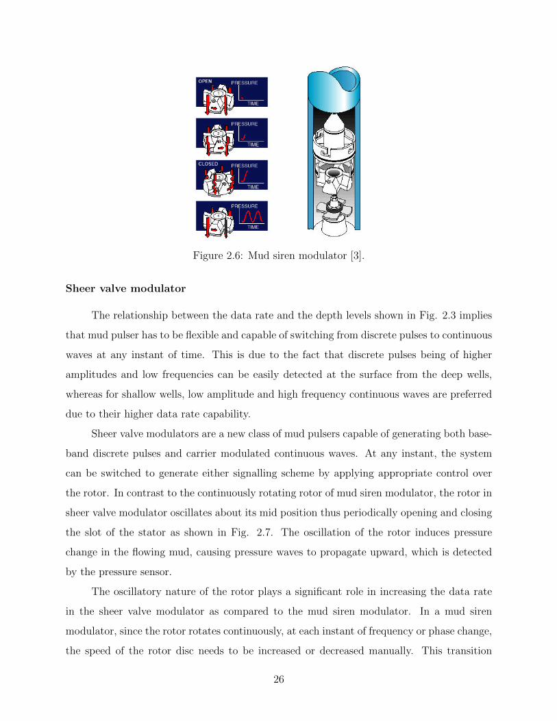
Figure 2.6: Mud siren modulator [3].

Sheer valve modulator

The relationship between the data rate and the depth levels shown in Fig. 2.3 implies

that mud pulser has to be flexible and capable of switching from discrete pulses to continuous

waves at any instant of time. This is due to the fact that discrete pulses being of higher

amplitudes and low frequencies can be easily detected at the surface from the deep wells,

whereas for shallow wells, low amplitude and high frequency continuous waves are preferred

due to their higher data rate capability.

Sheer valve modulators are a new class of mud pulsers capable of generating both base-

band discrete pulses and carrier modulated continuous waves. At any instant, the system

can be switched to generate either signalling scheme by applying appropriate control over

the rotor. In contrast to the continuously rotating rotor of mud siren modulator, the rotor in

sheer valve modulator oscillates about its mid position thus periodically opening and closing

the slot of the stator as shown in Fig. 2.7. The oscillation of the rotor induces pressure

change in the flowing mud, causing pressure waves to propagate upward, which is detected

by the pressure sensor.

The oscillatory nature of the rotor plays a significant role in increasing the data rate

in the sheer valve modulator as compared to the mud siren modulator. In a mud siren

modulator, since the rotor rotates continuously, at each instant of frequency or phase change,

the speed of the rotor disc needs to be increased or decreased manually. This transition

26

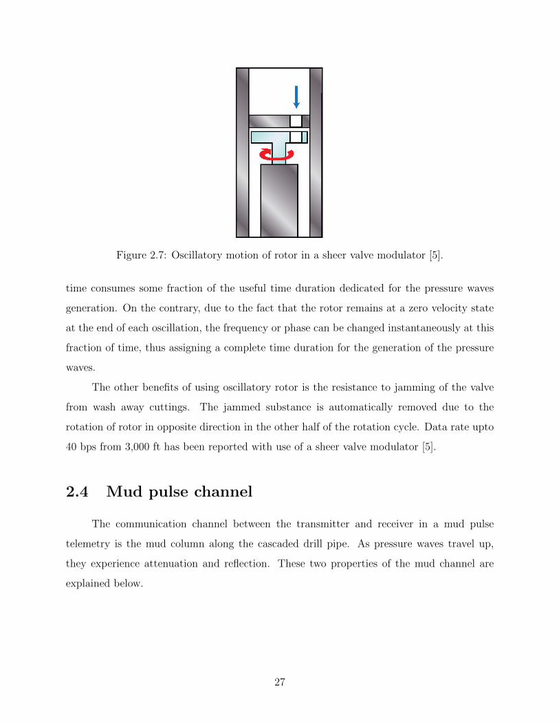
Figure 2.7: Oscillatory motion of rotor in a sheer valve modulator [5].

time consumes some fraction of the useful time duration dedicated for the pressure waves

generation. On the contrary, due to the fact that the rotor remains at a zero velocity state

at the end of each oscillation, the frequency or phase can be changed instantaneously at this

fraction of time, thus assigning a complete time duration for the generation of the pressure

waves.

The other benefits of using oscillatory rotor is the resistance to jamming of the valve

from wash away cuttings. The jammed substance is automatically removed due to the

rotation of rotor in opposite direction in the other half of the rotation cycle. Data rate upto

40 bps from 3,000 ft has been reported with use of a sheer valve modulator [5].

2.4 Mud pulse channel

The communication channel between the transmitter and receiver in a mud pulse

telemetry is the mud column along the cascaded drill pipe. As pressure waves travel up,

they experience attenuation and reflection. These two properties of the mud channel are

explained below.

27

Attenuation

Attenuation is the fundamental distance dependent property of the mechanical waves.

In mud pulse telemetry, the attenuation of the pressure waves increases with the depth

travelled by the pressure waves, smaller internal diameter of the pipe, viscosity and com-

pressibility of the mud. Since the viscosity of the mud decreases with rise in temperature, the

pressure wave attenuation is high at lower temperatures. Also, pressure wave attenuation

increases with the increase in frequency of the propagating wave. It is due to this reason deep

wells use low frequency pressure waves while shallow wells prefer higher frequency pressure

waves.

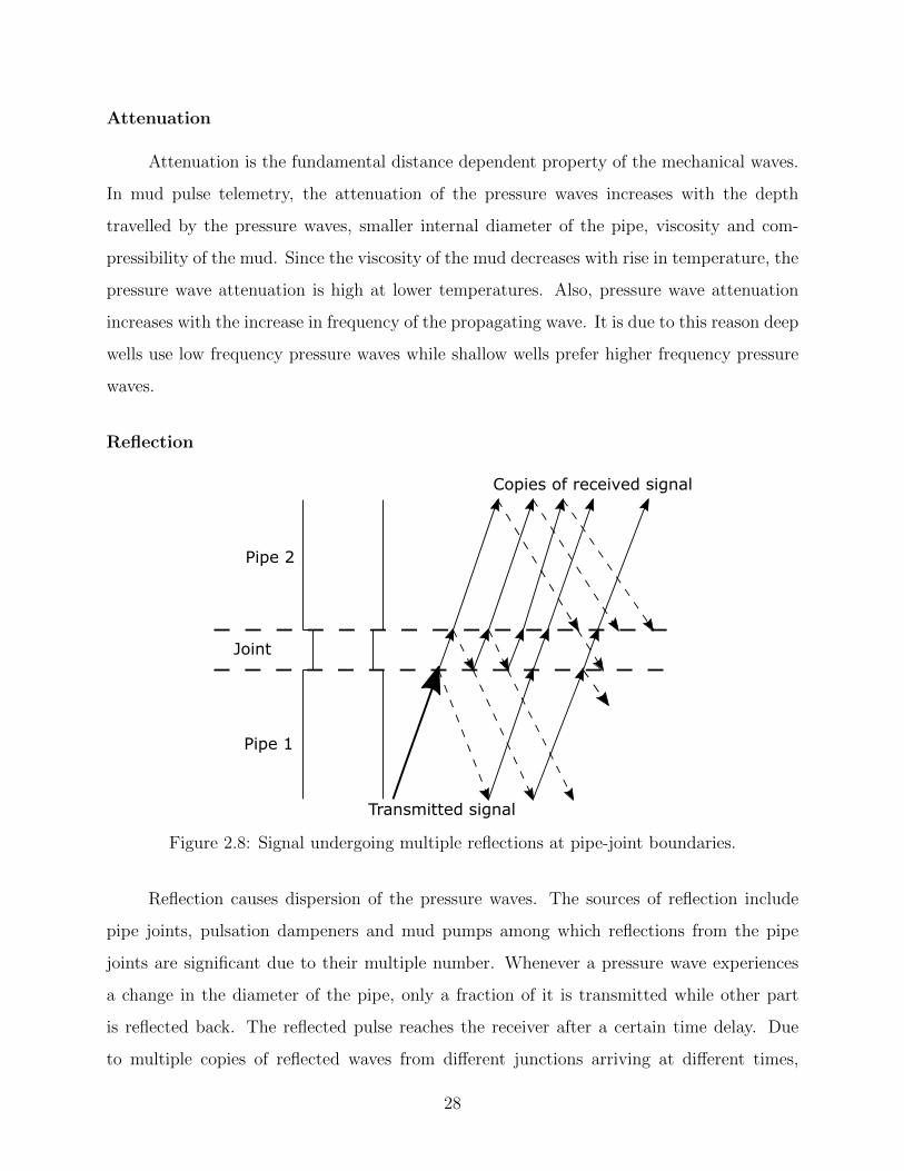
Reflection

Pipe 1

Pipe 2

Joint

Transmitted signal

Copies of received signal

Figure 2.8: Signal undergoing multiple reflections at pipe-joint boundaries.

Reflection causes dispersion of the pressure waves. The sources of reflection include

pipe joints, pulsation dampeners and mud pumps among which reflections from the pipe

joints are significant due to their multiple number. Whenever a pressure wave experiences

a change in the diameter of the pipe, only a fraction of it is transmitted while other part

is reflected back. The reflected pulse reaches the receiver after a certain time delay. Due

to multiple copies of reflected waves from different junctions arriving at different times,

28

the receiver may perform an erroneous detection thus, degrading the system performance.

Fig. 2.8 shows a pressure wave signal reflected from two boundaries of a pipe-joint where

solid lines refer to the waves travelling up whereas the dotted lines represent reflected waves

travelling down the pipe. The received signal is the superposition of the original signal with

multiple delayed and attenuated version of itself.

Authors in [17] have provided a mathematical model of the mud channel characteristics

at different frequencies. However, their model only account for pressure wave attenuation

and does not consider the reflection phenomenon of pressure waves from the junction of

the pipe boundaries. A comprehensive description of the attenuation of the mud pulses

based on the fluid transmission line concept will be covered in Chapter 3. The developed

attenuation model incorporates mud properties and is frequency dependent. It also includes

the effect of the reflection phenomena of the pressure waves. Thus, effects of mud properties

and frequency on the mud pulse propagation as well as the reflection properties of the mud

channel can be easily obtained from the fluid transmission line model.

2.5 Noise in a mud pulse communication system

In mud pulse telemetry, noise is added to the transmitted signal both from the downhole

and from the surface. In this thesis, it has been assumed that the noise from the downhole is

wide-band and gaussian in nature. Such a wide-band gaussian noise includes thermal noise

from the downhole electronics and noise from the vibration of the entire downhole assembly

or simply from the vibration of the drill pipes [36]. These vibrations induced gaussian noise

may lead to low SNR at the receiver. This thesis does not provide the characteristics of

such vibrations induced gaussian noise. However, the generated gaussian noise is scaled

in the simulation in later chapters to imply that the additive gaussian noise includes the

summation of these two gaussian noise generated from different sources. Therefore, only

thermally generated gaussian noise will be discussed here. Noise from the surface are due to

mud pumps and are narrow-band in nature.

29

2.5.1 Wide-band thermal noise

Thermal noise is an electrical noise due to random vibration of electrons within an

electronic circuit. It is ubiquitous in every communication system and follows a gaussian

distribution. Since power spectral density of such noise is constant over a wide range of

frequencies, it is also called broad-band noise. The two-sided power spectral density is flat

and is given as

S(f) =No

2watts/Hz, (2.3)

where

No = KTe,

K=Boltzman’s constant (1.38 ∗ 10−23 J/k),

Te=Equivalent noise temperature (k).

As given by (2.3), theoretically, thermal noise has an infinite average power. However, their

effect is realized once they pass through a system having a finite bandwidth.

The auto-correlation function of the thermal noise is a delta function given by

R(τ) =No

2δ(τ). (2.4)

From (2.4), it is noted that any two samples of the thermal noise are uncorrelated.

2.5.2 Narrow-band mud pump noise

In mud pulse telemetry, mud is circulated into the drilling rig via one or more than one

large powerful mud pumps capable of generating high pressure and flow rate. These mud

pumps are reciprocating in nature, i.e. one side of the piston/cylinder moves back to take

in drilling mud through an input valve while other side pushes drilling mud forward through

an output valve. Depending on the number of pistons available, mud pumps are classified

as duplex, triplex or hex pumps [58]. Mud pumps are further classified on the basis of the

number of working ends each piston has, e.g. a single action mud pump has each piston

capable of pumping mud in just one direction, whereas a double action mud pump has each

piston capable of pumping mud in both directions.

30

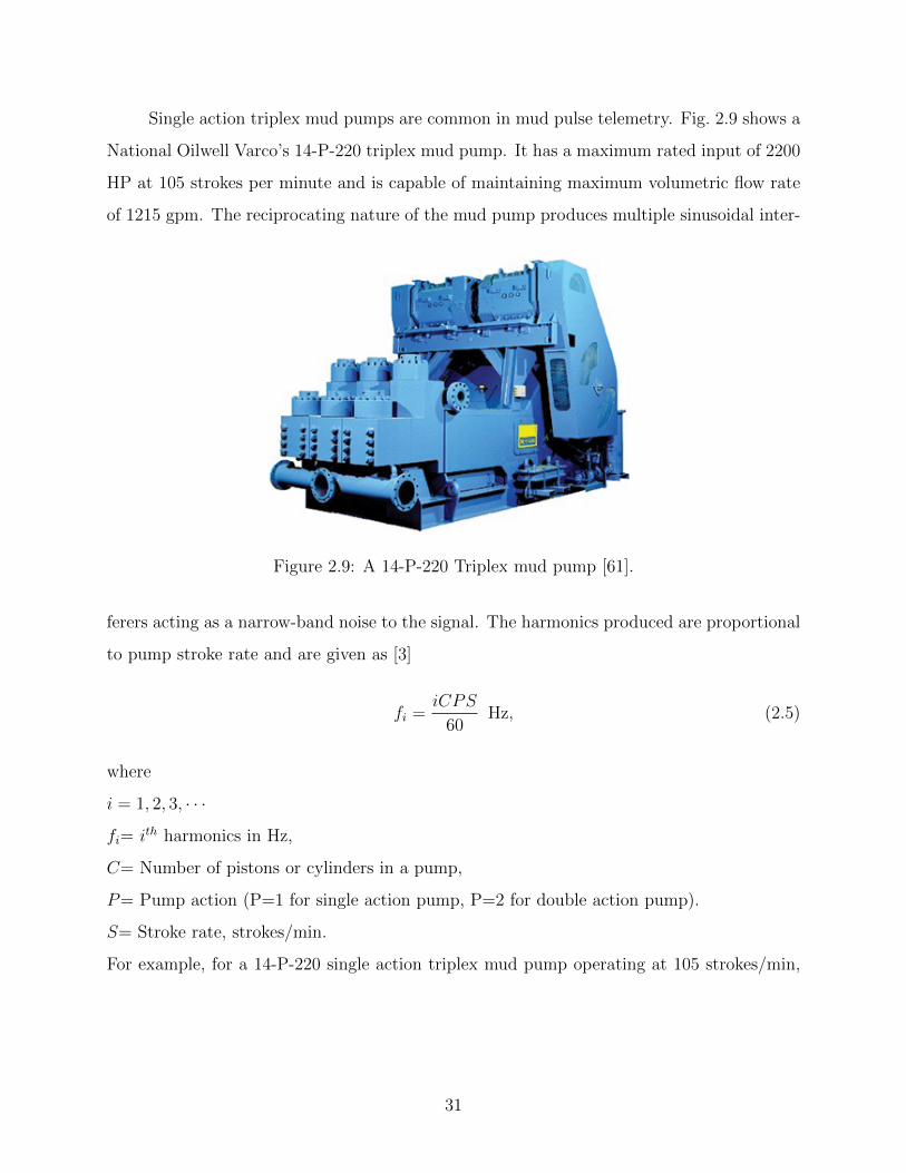
Single action triplex mud pumps are common in mud pulse telemetry. Fig. 2.9 shows a

National Oilwell Varco’s 14-P-220 triplex mud pump. It has a maximum rated input of 2200

HP at 105 strokes per minute and is capable of maintaining maximum volumetric flow rate

of 1215 gpm. The reciprocating nature of the mud pump produces multiple sinusoidal inter-

Figure 2.9: A 14-P-220 Triplex mud pump [61].

ferers acting as a narrow-band noise to the signal. The harmonics produced are proportional

to pump stroke rate and are given as [3]

fi =iCPS

60Hz, (2.5)

where

i = 1, 2, 3, · · ·

fi= ith harmonics in Hz,

C= Number of pistons or cylinders in a pump,

P= Pump action (P=1 for single action pump, P=2 for double action pump).

S= Stroke rate, strokes/min.

For example, for a 14-P-220 single action triplex mud pump operating at 105 strokes/min,

31

the fundamental frequency and harmonics generated can be calculated as

fi =i× 3× 1× 105

60

= 5.25i Hz.

5 10 15 20 25

Frequency(Hz)

10-30

10-20

10-10

100

Mag

nitu

de(d

B)

Figure 2.10: Power spectral density of mud pump noise harmonics.

Thus, the fundamental noise frequency is at 5.25 Hz and the harmonics occur at 10.5

Hz, 15.75 Hz and so on. These frequencies are shown in the power spectrum of the mud

pump noise in Fig. 2.10 where only three dominant harmonics have been plotted. Usually

for the mud pumps in perfect operating conditions, the amplitude of fundamental frequency

is much larger than harmonics, whereas for the mud pumps in poor condition, harmonics

have larger amplitudes [3]. It is therefore, for the plot of power spectrum in Fig. 2.10, the

amplitude of fundamental frequency is set to 10 volts where as the harmonics are set to have

amplitudes of 2, 0.1 and 0.005 volts respectively. The phase of each random sinusoids is

assumed to be uniformly distributed between 0 and 2π.

32

2.6 Mud pulse receiver

In mud pulse telemetry, the receiver has a task of correctly decoding the downhole

data, thus, various signal processing techniques are used to reduce the bit error rate. Some

of these techniques include receiver matched filtering, interferer cancellation and channel

equalization. The details of such methods will be given in the chapters to follow. In this

section, an introduction to the pressure transducer is given, which is used to sense the

downhole pressure variations.

2.6.1 Standpipe transducer

A standpipe pressure transducer is an assembly of a solid metal pipe connected to the

drill string at the surface. Generally, it is located few feets from the mud pumps [48] as shown

in Fig. 2.1. Inside the metal pipe, the pressure sensor is present. When the information

carrying pressure wave in the mud passes through the pressure sensor, a highly sensitive

diaphragm inside the sensor senses the variation of the pressure and produces an equivalent

electrical voltage. The voltage signal is then sent to the surface signal processing receiver

via an electrical connection.

In the existing literature of mud pulse propagation, it has been shown that placing

multiple transducers at specific locations on the drill string turns out to be advantageous.

Authors in [48] and [49] have shown that using multiple pressure sensors more statistical

information of received signal is obtained, which can be used to cancel out interferers or

enhance the desired signal at the receiver. However, the effect of the exact location of a

pressure transducer on the data rate is underestimated. It will be shown in the subsequent

chapters that the location of a pressure sensor in fact affects the frequency response nature

of the mud channel and thus affects the maximum data rate achieved by the mud pulse

telemetry system.

33

Chapter 3

Mud pulse channel model and noise

In this chapter, a detailed analysis of the mud pulse telemetry (MPT) channel is pre-

sented. Section 3.1 introduces a fluid transmission line concept, which forms the basis of

our analysis. After justifying the equivalence between the fluid and electrical systems, the

solution of the pressure and flow rate at any point along a mud pulse channel is derived in

Section 3.2. In Section 3.3, the attenuation characteristics of a mud channel is derived, which

is based on the distributed parameters of a fluid transmission line. The derived attenuation

characteristics using the fluid transmission line model is verified with the experimentally

verified attenuation model of [17], which is based on Lamb’s law of pressure attenuation.

Similar to a cascaded electrical transmission line, Section 3.4 shows that a mud pulse chan-

nel can be represented by cascaded drill pipes. Section 3.5 derives a transfer function of a

mud channel. First, a transfer function equation is derived considering a single long pipe, i.e.

neglecting junction lengths. Next, a more general equation of transfer function is derived,

which includes the length of the junction connecting two drill pipes. Finally the effect of the

transducer location on the frequency response of a mud channel is provided in Section 3.6.

3.1 Fluid transmission line model

A fluid transmission line is an equivalence of an electrical transmission line that com-

pletely describes the dynamic behaviour of the fluid flow in an open or closed conduit. In mud

pulse telemetry, as pressure waves propagate through the fluid, such a model is necessary

34

to establish the mathematical model of a mud communication channel. The propagation of

a pressure wave signal through the fluid channel is affected by the mud parameters such as

mud viscosity, density and bulk modulus. By incorporating their effects in the pressure wave

propagation, a mud pulse telemetry channel is characterized. In order to describe the fluid

transmission line in the light of a standard electrical transmission line theory, it is necessary

to understand the similarities between these two systems and the basic distributed elements

which make the fluid transmission line.

3.1.1 Analogy between elements of hydraulic and electrical system

When fluid flows through a conduit, its behaviour is similar to the flow of current

through a conductor. Just like current flows when a potential difference is applied across the

two ends of a conductor, fluid flows when pressure difference occurs across the two ends of

a conduit. Thus, pressure difference-voltage difference and flow rate-current form analogous

pairs when comparing the nature of both systems. A DC voltage source such as a battery

or an AC voltage source such as an alternator drives current in an electric circuit whereas a

mechanical source such as a pump produces pressure difference necessary to flow fluid in a

hydraulic system. Of course the analogy applies to both liquid and pneumatic flow, however,

heretofore liquid flow through a circular tube will be assumed in all cases as it is the case of

the mud flow through a drill pipe.

In drilling, a hydraulic transmission line is a long tubular structure of drill pipes through

which mud flows due to the difference in pressure at both ends. In case of electrical trans-

mission lines, the line parameters (resistance, inductance and capacitance) are distributed

continuously along the line varying both with time and position. This is due to the fact that

the wavelength of the propagating wave is in the range of the physical dimensions of the

circuit elements, hence, current and voltage vary with position and time along the length of

a transmission line. Similarly, in a hydraulic transmission line, the line parameters can be

assumed to vary accordingly. Thus, similar to the method of obtaining the general solution

of the voltage and current along any point in an electrical transmission line, the solution of

the pressure and flow rate at any point along the hydraulic line can be obtained by solving a

set of partial differential equations by applying necessary boundary conditions. The solution

35

describes the pressure and flow rate as a complex function of distributed elements and is

frequency dependent.

3.1.2 Distributed elements of an MPT transmission line

Resistance, inertance1 and capacitance are the basic distributed elements of a mud

pulse telemetry transmission line. These elements are directly dependent on the mud prop-

erties and the small-signal performance of such distributed system depends on the frequency

at which the mud pulse signal propagates, hence, these elements link the physical property

of the mud with the propagation of pressure waves and help to describe the steady-state

frequency response of the oscillating pressure waves in terms of mud parameters. The dis-

tributed parameters of a mud pulse telemetry channel along with their governing equations

are described below.

Fluid resistance

The viscous nature of the mud opposes the flow in a drill pipe. To overcome this, more

pressure needs to be applied by the mud pump. Thus, a linear relationship between pressure

difference and flow rate can be written as

∆P = RQl, (3.1)

where

∆P = pressure difference across two ends of a pipe (Nm−2),

R= fluid resistance per unit length (kgm−5s−1),

Q= volume flow rate through a pipe (m3s−1),

l= length of a pipe section (m).

The fluid resistance depends on the nature of the fluid flow. Depending upon Reynolds

number the flow is classified as laminar or turbulent. Resistance in laminar flow is given by

Hagen-Poiseuille equation and in turbulent flow is given by Darcy-Weisbach relation [16].

1In fluid terminology, inductance is commonly termed as inertance as it occurs due to inertia of theflowing fluid.

36

Both of these relations however ignore the effect of the frequency of the propagating pressure

waves and thus are applicable only for approximating very low frequency pressure wave

propagation (< 0.5 Hz). When the drilling fluid oscillates at a medium to high frequencies,

the concentration of the flow becomes significant at the boundary region, a phenomenon

similar to the skin effect in high-frequency AC propagation in an electrical transmission line.

Thus, resistance in fluid varies with a change in propagating frequency of the pressure waves

through the drilling fluid. The frequency dependent viscous resistance based on skin depth

has been described in detail in [13] and further simplified approximations of the results are

made in [14]. A characteristic frequency separating low frequency and high frequency flow

regime is given as

ωv =8πv

A, (3.2)

where

v= kinematic viscosity of the fluid (m2s−1),

A= cross sectional area of a pipe (m2).

Based on this characteristic frequency, the viscous resistance per unit length of the pipe is

expressed as [14]

R =ρ√ωvω

2A, (3.3)

where

ρ= mud density (kgm−3),

ω = angular frequency (rads−1).

Fluid inertance

An incompressible fluid offers inertia as it flows through the narrow pipe of uniform

cross section. The momentum generated by the flowing fluid can be expressed using the

equation of motion as [9]

∆P = ρldv

dt, (3.4)

37

where

v= mean fluid velocity (ms−1).

Rearranging (3.4) and using the relation v = Q/A, we get

∆P =ρl

A

dQ

dt

or

∆P = LldQ

dt. (3.5)

In (3.5), the term L = ρ/A gives fluid inertance per unit length of a pipe.

Fluid capacitance

Fluid capacitance arises due to compressible nature of the fluid, as with increased

pressure more fluid can be stored in a given volume. The fluid capacitance is obtained from

the continuity equation as [9]

dv =l

Beff

dP

dt, (3.6)

where

dv= difference of mean velocity at the two ends of a pipe,

dP= pressure difference at the two ends of a pipe,

Beff= effective bulk modulus of a fluid in a uniform pipe which is given as [17]

Beff =BM

B + M(3.7)

and

M =E(a2 − b2)

4b2(54− λ) + 2(1 + λ)(a2 + b2)

, (3.8)

where

B= bulk modulus of the mud (Nm−2),

E= Young’s modulus of elasticity of a drill pipe (Nm−2),

a= Outer diameter of a drill pipe (m),

b= Inner diameter of a drill pipe (m),

38

λ= Poisson ratio of the pipe material.

Rearranging the terms of (3.6) gives

dQ =Al

Beff

dP

dt

or

dQ = CldP

dt. (3.9)

In (3.9), the term C = A/Beff represents the fluid capacitance per unit length of a pipe.

3.2 General solution of the pressure and flow rate in

an MPT transmission line

+

_

P(x+ x,t)x

Q(x,t) (x+ x,t)

P(x,t)

+

_

R x L x

C

Q

Figure 3.1: An electrical equivalence of an infinitesimal segment of a drill pipe.

Consider an infinitesimal segment of a drill pipe of length ∆x. This small length

can be approximated with a lumped model of a transmission line as shown in Fig. 3.1.

The resistance R∆x accounts for the loss as the wave propagates through the pipe, the

inductance L∆x denotes the total fluid inertance and the capacitance C∆x represents total

compressibility of the fluid for length ∆x.

Let P (x, t) and P (x + ∆x, t) denote the pressure at the two ends of the infinitesimal

pipe with the corresponding flow rates at both ends as Q(x, t) and Q(x+ ∆x, t) respectively.

Both pressure and flow rates are the functions of position and time. With an analogy to the

39

electrical transmission line model, the relationship between pressure difference at the two

ends of the infinitesimal section can be written as

P (x, t)− P (x+ ∆x, t) = R∆xQ(x, t) + L∆x∂Q(x, t)

∂t. (3.10)

Dividing by ∆x and as ∆x→ 0

∂P (x, t)

∂x= −RQ(x, t)− L∂Q(x, t)

∂t. (3.11)

Similarly, the relation between flow rates differences at two end of the infinitesimal section

can be written as

Q(x, t)−Q(x+ ∆x, t) = C∆x∂P (x+ ∆x, t)

∂t. (3.12)

Dividing by ∆x and as ∆x→ 0

∂Q(x, t)

∂x= −C∂P (x, t)

∂t. (3.13)

Since, both pressure and flow rates are the functions of position and time, we can express

these quantities in phasor form as

P (x, t) = Re[P (x)ejωt] (3.14)

and

Q(x, t) = Re[Q(x)ejωt]. (3.15)

Substituting (3.14) and (3.15) in (3.11), we get

Re

[∂P (x)ejωt

∂x

]= −RRe[Q(x)ejωt]− LRe[Q(x)jωejωt]

which can be written as

Re

[(dP (x)

dx+ (R + jωL)Q(x)

)ejωt]

= 0.

40

Therefore,dP (x)

dx= −(R + jωL)Q(x). (3.16)

Similarly, substituting (3.14) and (3.15) in (3.13), we get

dQ(x)

dx= −jωCP (x). (3.17)

Now, differentiating (3.16) with respect to x and substituting (3.17) we get,

d2P (x)

dx2= (R + jωL)jωCP (x)

ord2P (x)

dx2− γ2P (x) = 0, (3.18)

where γ =√jωC(R + jωL) is known as the propagation constant.

The general solution of (3.18) can be written as

P (x) = Ae−γx +Beγx. (3.19)

Similarly, for the flow rate, the solution can be obtained by substituting (3.19) in (3.17).

This givesdQ(x)

dx= −jωC[Ae−γx +Beγx]. (3.20)

Integrating (3.20),

Q(x) =−jωCγ

[−Ae−γx +Beγx

]or

Q(x) =1

Zc

[Ae−γx −Beγx

], (3.21)

where Zc =√

R+jωLjωC

is the characteristic impedance. To solve the unknowns A and B, we

apply the boundary conditions. At x = 0, i.e. at the sending end,

P (0) = Ps = A+B (3.22)

41

and

Q(0) = Qs =1

Zc[A−B], (3.23)

where Ps and Qs represent pressure and flow rate at the source respectively. Solving (3.22)

and (3.23), we get

A =Ps + ZcQs

2

and

B =Ps − ZcQs

2.

The resultant pressure and flow rate then becomes

P (x) =Ps + ZcQs

2e−γx +

Ps − ZcQs

2eγx (3.24)

and

Q(x) =1

Zc

Ps + ZcQs

2e−γx − 1

Zc

Ps − ZcQs

2eγx. (3.25)

At receiving end, x = l, P (l) = Pr and Q(l) = Qr. Thus,

Pr =Ps + ZcQs

2e−γl +

Ps − ZcQs

2eγl (3.26)

and

Qr =1

Zc

Ps + ZcQs

2e−γl − 1

Zc

Ps − ZcQs

2eγl. (3.27)

The hyperbolic form of pressure and flow rate relation becomes

Pr = Ps cosh(γl)− ZcQs sinh(γl) (3.28)

and

Qr =−Ps

Zcsinh(γl) +Qs cosh(γl). (3.29)

42

In a matrix form, the pressure and flow rate relationship can be written as Ps

Qs

=

cosh(γl) Zc sinh(γl)

1Zc

sinh(γl) cosh(γl)

Pr

Qr

. (3.30)

Equivalently, Pr

Qr

=

cosh(γl) −Zc sinh(γl)

−1Zc

sinh(γl) cosh(γl)

Ps

Qs

, (3.31)

where cosh(γl) = eγl+e−γl

2and sinh(γl) = eγl−e−γl

2.

3.3 Attenuation characteristics of an MPT channel

Equation (3.24) gives the resultant pressure at any point along a pipe in terms of source

pressure. Substituting the values of cosh(γl), sinh(γl) and using the relation Ps = ZcQs in

(3.28) gives

Pr = Pse−γl, (3.32)

where the propagation constant can be written as

γ = α + jβ =√

(R + jωL)jωC. (3.33)

In (3.33), α is the attenuation constant in neper/meter and β is the phase constant in

radian/meter. Equation (3.32) shows that the pressure wave decays exponentially as it

propagates away from the source in a drill pipe. Squaring both sides and separating real and

imaginary parts in (3.33), we get

α2 − β2 = −ω2LC (3.34)

2αβ = ωRC. (3.35)

Solving for α gives

α =

√−ω2LC +

√ω4L2C2 + ω2R2C2

2. (3.36)

43

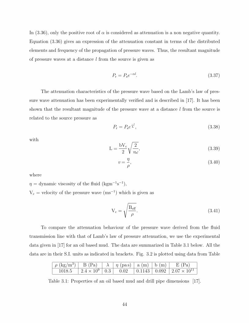
In (3.36), only the positive root of α is considered as attenuation is a non negative quantity.

Equation (3.36) gives an expression of the attenuation constant in terms of the distributed

elements and frequency of the propagation of pressure waves. Thus, the resultant magnitude

of pressure waves at a distance l from the source is given as

Pr = Pse−αl. (3.37)

The attenuation characteristics of the pressure wave based on the Lamb’s law of pres-

sure wave attenuation has been experimentally verified and is described in [17]. It has been

shown that the resultant magnitude of the pressure wave at a distance l from the source is

related to the source pressure as

Pr = Pse−lL , (3.38)

with

L =bVc

2

√2

vω, (3.39)

v =η

ρ, (3.40)

where

η = dynamic viscosity of the fluid (kgm−1s−1),

Vc = velocity of the pressure wave (ms−1) which is given as

Vc =

√Beff

ρ. (3.41)

To compare the attenuation behaviour of the pressure wave derived from the fluid

transmission line with that of Lamb’s law of pressure attenuation, we use the experimental

data given in [17] for an oil based mud. The data are summarized in Table 3.1 below. All the

data are in their S.I. units as indicated in brackets. Fig. 3.2 is plotted using data from Table

ρ (kg/m3) B (Pa) λ η (pa s) a (m) b (m) E (Pa)1018.5 2.4× 109 0.3 0.02 0.1143 0.092 2.07× 1011

Table 3.1: Properties of an oil based mud and drill pipe dimensions [17].

44

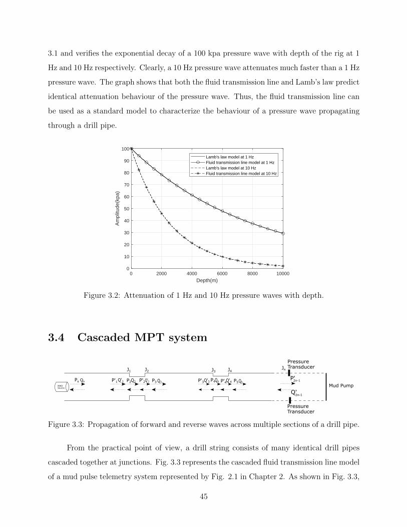
3.1 and verifies the exponential decay of a 100 kpa pressure wave with depth of the rig at 1

Hz and 10 Hz respectively. Clearly, a 10 Hz pressure wave attenuates much faster than a 1 Hz

pressure wave. The graph shows that both the fluid transmission line and Lamb’s law predict

identical attenuation behaviour of the pressure wave. Thus, the fluid transmission line can

be used as a standard model to characterize the behaviour of a pressure wave propagating

through a drill pipe.

0 2000 4000 6000 8000 10000

Depth(m)

0

10

20

30

40

50

60

70

80

90

100

Am

plitu

de(k

pa)

Lamb's law model at 1 HzFluid transmission line model at 1 HzLamb's law model at 10 HzFluid transmission line model at 10 Hz

Figure 3.2: Attenuation of 1 Hz and 10 Hz pressure waves with depth.

3.4 Cascaded MPT system

J1 J2 J3 J4

P'1Ps P2 P3 P'3 P4 P5Qs Q'1 Q2 P'2Q'2 Q3 Q'3 Q4 P'4Q'4 Q5

MWDSource

Jn

2n-1

2n-1

Pressure Transducer

Pressure Transducer

Mud Pump

P'

Q'

Figure 3.3: Propagation of forward and reverse waves across multiple sections of a drill pipe.

From the practical point of view, a drill string consists of many identical drill pipes

cascaded together at junctions. Fig. 3.3 represents the cascaded fluid transmission line model

of a mud pulse telemetry system represented by Fig. 2.1 in Chapter 2. As shown in Fig. 3.3,

45

at each junction, the diameter of a drill string is lower than subsequent pipe sections due

to threads used to connect two pipes together. The pressure wave generated by the MWD

signal source travels in both forward and reverse direction. As the wave propagates along the

drill string, it gets attenuated. Besides, the discontinuity in the diameter causes reflection of

the pressure waves in either direction. Thus, the pressure transducer located along the pipe

section receives both transmitted and reflected pressure waves leading to signal dispersion.

Let the drill string consists of K pipe-junction sections. Ps and Qs represent the

source pressure and flow rate respectively. At any arbitrary pipe or junction k, let Pk and

Qk represent the pressure and flow rate at the input of kth pipe or junction while P ′k and Q′k

denote their corresponding values at the output. We assume the standpipe transducer to be

located at the end of nth junction so that P ′2n−1 and Q′2n−1 are the pressure and flow rate

values at the pressure transducer.

Using (3.31), the pressure and flow rate at the end of the first pipe section are related

to source pressure and flow rate as P ′1

Q′1

=

cosh(γplp) −Zp sinh(γplp)

−1Zp

sinh(γplp) cosh(γplp)

Ps

Qs

. (3.42)

Similarly, at the end of first junction section, the pressure and flow rates are expressed as P ′2

Q′2

=

cosh(γj lj) −Zj sinh(γj lj)

−1Zj

sinh(γj lj) cosh(γj lj)

P2

Q2

. (3.43)

Now, using the condition of continuity of pressure and flow at junction J1, we have, P ′1 = P2

and Q′1 = Q2.

Using this relation in (3.43) and substituting (3.42), we get

P ′2

Q′2

=

cosh(γj lj) −Zj sinh(γj lj)

−1Zj

sinh(γj lj) cosh(γj lj)

cosh(γplp) −Zp sinh(γplp)

−1Zp

sinh(γplp) cosh(γplp)

Ps

Qs

.(3.44)

Similarly, at the end of Junction J2, P ′2 = P3 and Q′2 = Q3.

46

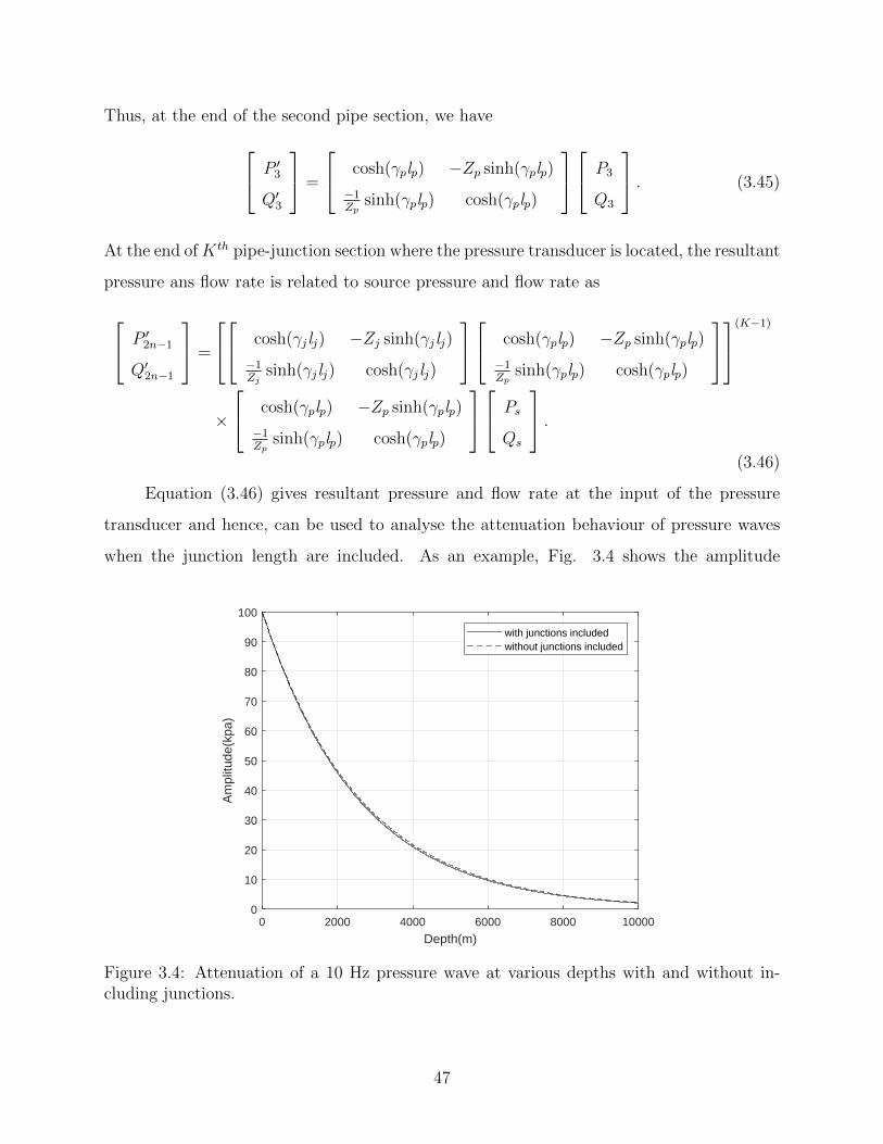
Thus, at the end of the second pipe section, we have P ′3

Q′3

=

cosh(γplp) −Zp sinh(γplp)

−1Zp

sinh(γplp) cosh(γplp)

P3

Q3

. (3.45)

At the end ofKth pipe-junction section where the pressure transducer is located, the resultant

pressure ans flow rate is related to source pressure and flow rate as

P ′2n−1

Q′2n−1

=

cosh(γj lj) −Zj sinh(γj lj)

−1Zj

sinh(γj lj) cosh(γj lj)

cosh(γplp) −Zp sinh(γplp)

−1Zp

sinh(γplp) cosh(γplp)

(K−1)

×

cosh(γplp) −Zp sinh(γplp)

−1Zp

sinh(γplp) cosh(γplp)

Ps

Qs

.(3.46)

Equation (3.46) gives resultant pressure and flow rate at the input of the pressure

transducer and hence, can be used to analyse the attenuation behaviour of pressure waves

when the junction length are included. As an example, Fig. 3.4 shows the amplitude

0 2000 4000 6000 8000 10000

Depth(m)

0

10

20

30

40

50

60

70

80

90

100

Am

plitu

de(k

pa)

with junctions includedwithout junctions included

Figure 3.4: Attenuation of a 10 Hz pressure wave at various depths with and without in-cluding junctions.

47

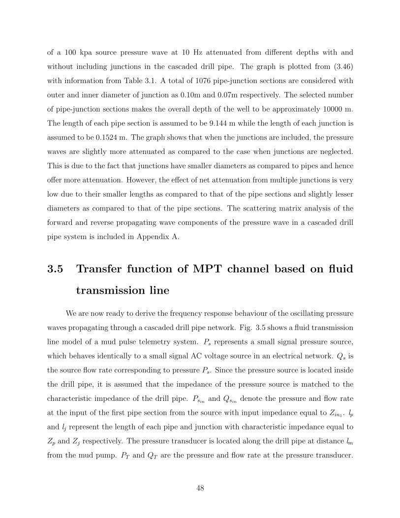
of a 100 kpa source pressure wave at 10 Hz attenuated from different depths with and

without including junctions in the cascaded drill pipe. The graph is plotted from (3.46)

with information from Table 3.1. A total of 1076 pipe-junction sections are considered with

outer and inner diameter of junction as 0.10m and 0.07m respectively. The selected number

of pipe-junction sections makes the overall depth of the well to be approximately 10000 m.

The length of each pipe section is assumed to be 9.144 m while the length of each junction is

assumed to be 0.1524 m. The graph shows that when the junctions are included, the pressure

waves are slightly more attenuated as compared to the case when junctions are neglected.

This is due to the fact that junctions have smaller diameters as compared to pipes and hence

offer more attenuation. However, the effect of net attenuation from multiple junctions is very

low due to their smaller lengths as compared to that of the pipe sections and slightly lesser

diameters as compared to that of the pipe sections. The scattering matrix analysis of the

forward and reverse propagating wave components of the pressure wave in a cascaded drill

pipe system is included in Appendix A.

3.5 Transfer function of MPT channel based on fluid

transmission line

We are now ready to derive the frequency response behaviour of the oscillating pressure

waves propagating through a cascaded drill pipe network. Fig. 3.5 shows a fluid transmission

line model of a mud pulse telemetry system. Ps represents a small signal pressure source,

which behaves identically to a small signal AC voltage source in an electrical network. Qs is

the source flow rate corresponding to pressure Ps. Since the pressure source is located inside

the drill pipe, it is assumed that the impedance of the pressure source is matched to the

characteristic impedance of the drill pipe. Psin and Qsin denote the pressure and flow rate

at the input of the first pipe section from the source with input impedance equal to Zin1 . lp

and lj represent the length of each pipe and junction with characteristic impedance equal to

Zp and Zj respectively. The pressure transducer is located along the drill pipe at distance lm

from the mud pump. PT and QT are the pressure and flow rate at the pressure transducer.

48

.

Pressure transducer

lm

Zin1.

Kth pipe

lp lj

PT

8

ZL=Mud pump(open circuit)

z=0

.Zp

Ps

Istpipe IstJunction

Psin

2ndpipe

,Wsin

`

Qs

2ndJunction

QT,

Pbottom Ptop

Figure 3.5: Cascaded drill pipe system, including junctions with pressure transducer alongthe drill pipe.

Since the mud pump is located at z = 0, all the distances are negative.

In order to represent the MPT structure with an equivalent fluid transmission line

model, certain assumptions are made. First, it is assumed that the mud pump maintains a

constant flow and thus acts as an analogous constant-current source. As such, it is identical

to an open circuit in an electrical system. Therefore, the input impedance at the mud pump

is assumed to be infinite, i.e. ZL =∞. Next, the signal grounds located at the small signal

pressure source Ps and the mud pump as shown in Fig. 3.5 represent the constant pressure

levels at the location of the drill bit and the mud pump. These constant pressure levels are

represented by Pbottom and Ptop respectively. The two constant pressure levels are related as

Pbottom = Ptop + Phydrostatic − Pfrictionalloss (3.47)

In (3.47), Ptop represents the constant pressure generated by the mud pump, Phydrostatic is

the excess pressure at the drill bit region due to the well depth and Pfrictionalloss represents

the pressure loss due to friction.

The constant pressure levels at the top and bottom region of the cascaded drill pipe

system result in a DC offset along with the small signal pressure generated by the modulator

valve. The DC offset only shifts the signal level about the zero frequency but does not alter

the nature of the transfer function of the mud channel defined as the function of frequencies.

Furthermore, the DC offset can be compensated by measuring the constant pressure levels

and subtracting them from the received pressure signal level. The nature of the transfer

function of the mud channel depends only upon the ratio of the small signal pressure at the

49

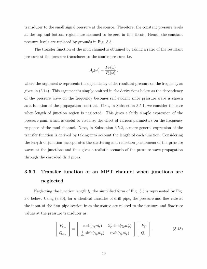
transducer to the small signal pressure at the source. Therefore, the constant pressure levels

at the top and bottom regions are assumed to be zero in this thesis. Hence, the constant

pressure levels are replaced by grounds in Fig. 3.5.

The transfer function of the mud channel is obtained by taking a ratio of the resultant

pressure at the pressure transducer to the source pressure, i.e.

Ap(ω) =PT (ω)

Ps(ω),

where the argument ω represents the dependency of the resultant pressure on the frequency as

given in (3.14). This argument is simply omitted in the derivations below as the dependency

of the pressure wave on the frequency becomes self evident since pressure wave is shown

as a function of the propagation constant. First, in Subsection 3.5.1, we consider the case

when length of junction region is neglected. This gives a fairly simple expression of the

pressure gain, which is useful to visualize the effect of various parameters on the frequency

response of the mud channel. Next, in Subsection 3.5.2, a more general expression of the

transfer function is derived by taking into account the length of each junction. Considering

the length of junction incorporates the scattering and reflection phenomena of the pressure

waves at the junctions and thus gives a realistic scenario of the pressure wave propagation

through the cascaded drill pipes.

3.5.1 Transfer function of an MPT channel when junctions are

neglected

Neglecting the junction length lj, the simplified form of Fig. 3.5 is represented by Fig.

3.6 below. Using (3.30), for n identical cascades of drill pipe, the pressure and flow rate at

the input of the first pipe section from the source are related to the pressure and flow rate

values at the pressure transducer as Psin

Qsin

=

cosh(γpnlp) Zp sinh(γpnlp)

1Zp

sinh(γpnlp) cosh(γpnlp)

PT

QT

, (3.48)

50

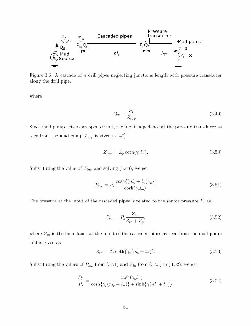
s

Zp Zin

8ZL=

.. .Mud pump

Pressure transducerCascaded pipes

nlp+

-

z=0

SourceMud

PPsin

Plm

TQTQsinQS

Figure 3.6: A cascade of n drill pipes neglecting junctions length with pressure transduceralong the drill pipe.

where

QT =PTZinT

. (3.49)

Since mud pump acts as an open circuit, the input impedance at the pressure transducer as

seen from the mud pump ZinT is given as [47]

ZinT = Zp coth(γplm). (3.50)

Substituting the value of ZinT and solving (3.48), we get

Psin = PTcosh{(nlp + lm)γp}

cosh(γplm). (3.51)

The pressure at the input of the cascaded pipes is related to the source pressure Ps as

Psin = PsZin

Zin + Zp, (3.52)

where Zin is the impedance at the input of the cascaded pipes as seen from the mud pump

and is given as

Zin = Zp coth{γp(nlp + lm)}. (3.53)

Substituting the values of Psin from (3.51) and Zin from (3.53) in (3.52), we get

PTPs

=cosh(γplm)

cosh{γp(nlp + lm)}+ sinh{γ(nlp + lm)}. (3.54)

51

The pressure gain (transfer function) is given as

Ap =PTPs.

The hyperbolic terms in the denominator of (3.54) can be reduced to get

Ap = e−γp(nlp+lm) cosh(γplm). (3.55)

Equivalently,

Ap =e−nγplp + e−γp(nlp+2lm)

2. (3.56)

Equation (3.55) gives an expression of the pressure gain in cascaded drill pipes assuming

the length of each junctions as zero.

3.5.2 Transfer function of an MPT channel when junctions are

included

The effect of reflections on the transfer function of a mud channel becomes apparent

by considering the length of junctions. As shown in Fig. 3.5, the pressure and flow rate at

the input and output of the first drill pipe can be related in a similar manner using relations

from (3.30) as

Ppin

Qpin

=

cosh(γplp) Zp sinh(γplp)

1Zp

sinh(γplp) cosh(γplp)

Ppout

Qpout

. (3.57)

Similarly, the pressure and flow rate at the input and output of the first junction segment

can be related as Pjin

Qjin

=

cosh(γj lj) Zj sinh(γj lj)

1Zj

sinh(γj lj) cosh(γj lj)

Pjout

Qjout

. (3.58)

Since the output of first pipe section acts as an input to the first junction section, for K such

pipe-junction sections, the input of the first pipe and the input to the transducer (i.e, output

52

of the kth pipe) are simply related by the chain multiplication of the adjacent matrices as

Psin

Qsin

=

cosh(γplp) Zp sinh(γplp)

1Zp

sinh(γplp) cosh(γplp)

cosh(γj lj) Zj sinh(γj lj)

1Zj

sinh(γj lj) cosh(γj lj)

(k−1)

×

cosh(γplp) Zp sinh(γplp)

1Zp

sinh(γplp) cosh(γplp)

PT

QT

,(3.59)

where

QT =PTZinT

. (3.60)

The impedance at the input of Kth pipe section from the mud pump can be written as

ZinK = Zp coth{γp(lm + lp)}. (3.61)

Similarly, the impedance at the input of (K − 1)th junction from the mud pump is given as

[47]

Zin(K−1)= Zj

ZinK + Zj tanh(γjlj)

Zj + ZinK tanh(γjlj). (3.62)

Thus, at the input of 1st pipe section, the input impedance can be written as

Zin1 = ZpZin2 + Zp tanh(γplp)

Zp + Zin2 tanh(γplp). (3.63)

Now, the pressure at the input of 1st section is related to source pressure Ps as

Psin = PsZin1

Zp + Zin1

(3.64)

or

Ps = PsinZp + Zin1

Zin1

. (3.65)

The pressure gain is thus

Ap =PTPs, (3.66)

where the value of Psin is obtained by substituting (3.60) in (3.59).

Fig. 3.7 shows transfer functions of a mud channel with and without including junc-

53

0 20 40 60 80 100

Frequency (Hz)

-350

-300

-250

-200

-150

-100

-50

0

Mag

nitu

de (

dB)

with junctions includedwithout junctions included

Figure 3.7: Transfer function of a cascaded drill pipe system with and without includingjunctions.

tions. The graph is plotted using (3.55) and (3.66) respectively with the data taken from

the Table 3.1. A total of 1076 pipe-junction sections are included. For the plot, each drill

pipe is assumed to be 9.144 m long with the outer and inner diameter as 0.1143 m and 0.092

m respectively, whereas each junction is assumed to be 0.1524 m long with the outer and

inner diameter as 0.10 m and 0.07 m respectively. The standpipe transducer is located at

a distance of 15.24 m from the mud pump [48]. At low frequencies, the effect of junctions

on the channel gain is negligible while at higher frequencies, the junctions slightly reduce

the channel gain. Also, the transfer function of the mud channel with junctions shows a

notch around 74.5 Hz. The notch formation is due to the effect of reflections from multiple

junctions.

3.6 Effect of the transducer location on mud channel

transfer function

The distance of the pressure transducer from the mud pump has an impact on the

nature of the frequency response of a mud communication channel. It is evident from (3.54)

that the distance lm determines the position of minima in the transfer function equation.

54

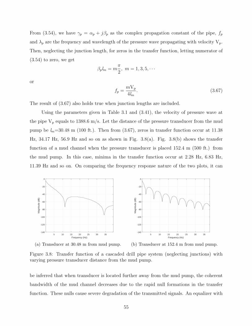
From (3.54), we have γp = αp + jβp as the complex propagation constant of the pipe, fp

and λp are the frequency and wavelength of the pressure wave propagating with velocity Vp.

Then, neglecting the junction length, for zeros in the transfer function, letting numerator of

(3.54) to zero, we get

βplm = mπ

2, m = 1, 3, 5, · · ·

or

fp =mVp

4lm. (3.67)

The result of (3.67) also holds true when junction lengths are included.

Using the parameters given in Table 3.1 and (3.41), the velocity of pressure wave at

the pipe Vp equals to 1388.6 m/s. Let the distance of the pressure transducer from the mud

pump be lm=30.48 m (100 ft.). Then from (3.67), zeros in transfer function occur at 11.38

Hz, 34.17 Hz, 56.9 Hz and so on as shown in Fig. 3.8(a). Fig. 3.8(b) shows the transfer

function of a mud channel when the pressure transducer is placed 152.4 m (500 ft.) from

the mud pump. In this case, minima in the transfer function occur at 2.28 Hz, 6.83 Hz,

11.39 Hz and so on. On comparing the frequency response nature of the two plots, it can

5 10 15 20 25 30 35

Frequency (Hz)

-140

-120

-100

-80

-60

-40

-20

0

Mag

nitu

de (

dB)

(a) Transducer at 30.48 m from mud pump.

5 10 15 20 25 30 35

Frequency (Hz)

-140

-120

-100

-80

-60

-40

-20

0

Mag

nitu

de (

dB)

(b) Transducer at 152.4 m from mud pump.

Figure 3.8: Transfer function of a cascaded drill pipe system (neglecting junctions) withvarying pressure transducer distance from the mud pump.

be inferred that when transducer is located further away from the mud pump, the coherent

bandwidth of the mud channel decreases due to the rapid null formations in the transfer

function. These nulls cause severe degradation of the transmitted signals. An equalizer with

55

a suitable number of taps is thus required to compensate the distortion caused by such nulls

in the mud channel.

56

Chapter 4

Receiver design and performance

analysis

This chapter focusses on the receiver design and its performance evaluation in a mud

pulse communication system. Various signal processing techniques aiming to reduce the bit

error rate at the receiver output have been described. Section 4.1 introduces a mud pulse

communication system and sets up various notations describing the transmitter, channel,

noise, interferers and receiver. The effect of narrowband interferers from the mud pump

on signal degradation has been elaborated in detail in Section 4.2. Section 4.3 presents an

adaptive filter capable of selectively cancelling out these narrow-band mud pump interferers.

Along with the design of such filter, its performance is analysed. Section 4.4 describes the

basics of channel equalization concept. In particular, the theory of Weiner filter and LMS

algorithm are summarized. Weiner filter will be used in the later chapter to compensate

the effect of signal distortion caused by the mud channel. Since, the adaptive notch filter

is designed with a modification to an LMS algorithm, the basics of the LMS algorithm is

summarized.

4.1 Structure of a receiver used in an MPT system

Fig. 4.1 shows a base-band structure of a mud pulse communication system. Ik repre-

sents the information symbol transmitted by the borehole electronics. Considering a simple

57

Downholedata

Modulator(pulser) g(t)

Mud Channel

mud pump interferersWhite gaussian noise n(t) and

Standpipe transducer (pressure sensor)

Adaptive notch filter hn(t)

s(t)

hc(t)

i(t)

y(t)x(t) Matched

filter hm(t)Ik Decision

device

Output dataEqualizer

sampling

z(kT+ )τ 0 ˆ dk

c(kT+ )τ 0

t=kT+τ 0

r(t)

Figure 4.1: Structure of a mud pulse communication system.

On-Off keying modulation scheme, these information symbols correspond to bits 1 and 0 re-

spectively. Modulator converts the information symbols 1 and 0 into corresponding pressure

waves s(t) with amplitudes ±1 respectively. Thus, the output of a modulator consists of a

train of pulses at a rate 1T

bps, where T represents symbol period. The transmitted pulse at

time t has a form

s(t) =∞∑k=0

Ikg(t− kT ), (4.1)

where g(t) represents the pressure pulse shape corresponding to the information sequence Ik.

The transmitted pressure waves propagate through mud as a channel. The impulse response

of the mud channel is denoted by hc(t). The output of the channel at time t is thus given as

x(t) =∞∑k=0

Ikv(t− kT ) + i(t) + n(t), (4.2)

where

v(t) =

∞∫−∞

s(τ)hc(t− τ)dτ (4.3)

represents the convolution of channel impulse response hc(t) and transmitted pressure wave

s(t), i(t) represents the narrow-band interferers and n(t) is the additive white gaussian noise.

The front end of a receiver unit placed at the surface includes a standpipe transducer,

which converts the pressure waves into equivalent voltage signals. A conventional receiver

design approach is followed in this section, which assumes an analog adaptive notch filter

followed by a matched filter. Thus, the received voltage signal acts as an input to an adaptive

notch filter hn(t) that cancels out the narrow-band interferers. The output of the notch filter

is

y(t) =

∞∫−∞

x(τ)hn(t− τ)dτ. (4.4)

58

The output of the notch filter is fed to the matched filter hm(t) matched to an overall

response of pulse shape and channel for a known channel. The received signal at the output

of matched filter is

r(t) =∞∑k=0

Ikw(t− kT ) + u(t), (4.5)

where

w(t) =

∞∫−∞

v(τ)hm(τ − t)dτ (4.6)

and

u(t) =

∞∫−∞

n(τ)hm(τ − t)dτ. (4.7)

In (4.6) and (4.7), v(t) and n(t) represent signal and noise components filtered by the notch

filter respectively. It is to be noted that this noise component includes the wideband channel

noise and the residues of narrow-band interferers that notch filter fails to remove.

The output r(t) of a matched filter is now sampled at some integral multiples of symbol

times t = mT + τ0, m = 0, 1, 2, · · · where τ0 denotes the transmission delay through the

channel. Thus, the output of the sampler is given as

r(mT + τ0) =∞∑k=0

Ikw(mT − kT + τ0) + u(mT + τ0). (4.8)

If an equalizer is assumed to have response c(mT + τ0) at time t=mT + τ0, the output esti-

mate of desired signal s(t) at time mT + τ0 is given as

z(mT + τ0) =∞∑

n=−∞

r(nT )c(mT + τ0 − nT ) + u(mT + τ0), (4.9)

where u(mT + τ0) represents filtered noise at the output of the equalizer.

59

4.2 Receiver performance degradation due to mud pump

interferers

Interferers generated from the mud pumps severely affect the receiver performance in

a mud pulse telemetry system. The interferers are narrow-band and can be represented

by sinusoids with phase distributed uniformly between 0 and 2π. As described in Chapter

2, the harmonics generated by the mud pump lie at integral multiples of the fundamental

frequency. It means that multiple additive interferers may corrupt the signal leading to a

high bit error rate at the receiver output. An expression for the bit error rate with interferers

derived in this section is adopted from [28], [29] and [30]. The final value of the probability

of a bit error is obtained by averaging over all possible random phases of all sinusoids.

4.2.1 Bit error rate expression with white noise and mud pump

interferers

The net interference i(t) from the mud pumps as shown in Fig. 4.1 can be expressed

as

i(t) =N∑n=1

an cos(2πfnt+ θn), (4.10)

where N is the total number of interferers, an is the nth interferer amplitude with frequency

fn, θn is the random phase of a nth interferer and is uniformly distributed between 0 and 2π.

The averaged interference at the output of a matched filter can be written as

i(t) =1

T

T∫0

i(t)dt

or

i(t) =1

T

T∫0

N∑n=1

an cos(2πfnt+ θn)dt, (4.11)

where T is the signal time period. In (4.11), it is assumed that the matched filter consists

of a square pulse matched to the signal pulse shape. Thus, the received signal sample at the

60

output of the matched filter at a sampling instant t = mT can be written as

r(mT ) = S + u(mT ) + i(mT ), (4.12)

where S is the signal amplitude equal to ±1 and u(mT ) is the white noise sample at the

matched filter output with one sided power spectral density equal to No. The probability

density function (PDF) of the received signal is gaussian distributed with its mean equal to

±S + i(kT ) and variance equal to σ2 = No2T

.

Let us assume the transmitter transmits symbol 1 corresponding to the signal amplitude

+S. In this case, the conditional PDF of the received signal for a given θn can be written as

fr|θn(r) =1√2πσ

exp

[−1

2σ2

{r − (S + i(mT ))

}2]. (4.13)

For a given θn, the conditional probability of error is given as

Pe1|θn = P (r < 0)

or

Pe1|θn =

0∫−∞

fr(r)dr

or

Pe1|θn =1

2erfc

[{S + i(mT )

}√T

√No

]. (4.14)

As θn are independent and uniformly distributed between 0 and 2π, the total unconditional

probability is the average of all θn over 0 to 2π. Therefore,

Pe1 =1

(2π)N

2π∫0

· · ·2π∫

0

Pe1|θdθ1 · · · dθN . (4.15)

When the transmitter transmits symbol 0 corresponding to signal amplitude −S, same form

61

of (4.14) and (4.15) are obtained as symbols 1 and 0 are equally likely. Thus,

Pe0|θn =1

2erfc

[{S + i(mT )

}√T

√No

], (4.16)

Pe0 =1

(2π)N

2π∫0

· · ·2π∫

0

Pe0|θdθ1 · · · dθN . (4.17)

The total error probability is then equal to

Pe = P (0)Pe0 + P (1)Pe1, (4.18)

where P (0) = P (1) = 12.

0 5 10 15

EbNo, dB

10-5

10-4

10-3

10-2

10-1

Bit

Err

or R

ate

theoretical BERsimulated BER

Figure 4.2: Bit error rate curve with a single narrowband interferer.

Fig. 4.2 shows theoretical and simulated bit error rate vs bit energy per noise power

spectral density (EbNo) curve for a single narrow-band sinusoid interferer. The theoretical

expression is plotted using (4.18). The signal is assumed to be a base-band square pulse of

amplitude 1 volt and frequency 10 Hz, whereas the interferer is a random phased sinusoid

of amplitude 0.7 volt with the frequency of 5.25 Hz.

62

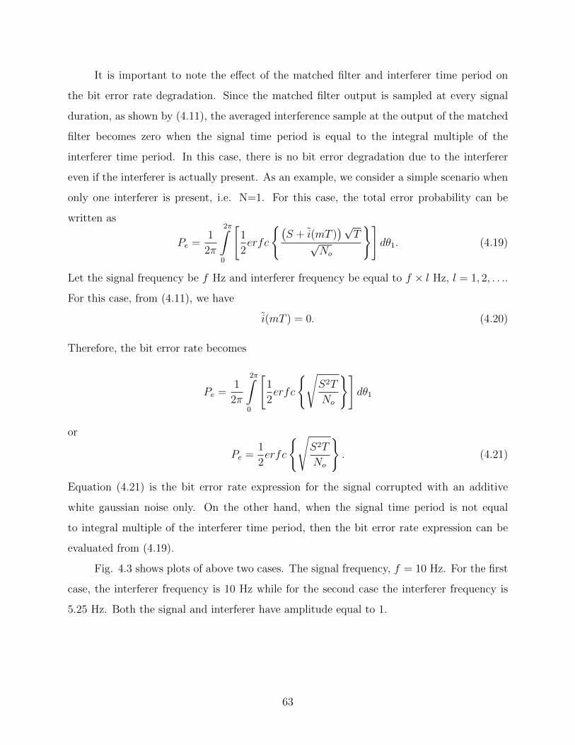
It is important to note the effect of the matched filter and interferer time period on

the bit error rate degradation. Since the matched filter output is sampled at every signal

duration, as shown by (4.11), the averaged interference sample at the output of the matched

filter becomes zero when the signal time period is equal to the integral multiple of the

interferer time period. In this case, there is no bit error degradation due to the interferer

even if the interferer is actually present. As an example, we consider a simple scenario when

only one interferer is present, i.e. N=1. For this case, the total error probability can be

written as

Pe =1

2π

2π∫0

[1

2erfc

{(S + i(mT )

)√T

√No

}]dθ1. (4.19)

Let the signal frequency be f Hz and interferer frequency be equal to f × l Hz, l = 1, 2, . . ..

For this case, from (4.11), we have

i(mT ) = 0. (4.20)

Therefore, the bit error rate becomes

Pe =1

2π

2π∫0

[1

2erfc

{√S2T

No

}]dθ1

or

Pe =1

2erfc

{√S2T

No

}. (4.21)

Equation (4.21) is the bit error rate expression for the signal corrupted with an additive

white gaussian noise only. On the other hand, when the signal time period is not equal

to integral multiple of the interferer time period, then the bit error rate expression can be

evaluated from (4.19).

Fig. 4.3 shows plots of above two cases. The signal frequency, f = 10 Hz. For the first

case, the interferer frequency is 10 Hz while for the second case the interferer frequency is

5.25 Hz. Both the signal and interferer have amplitude equal to 1.

63

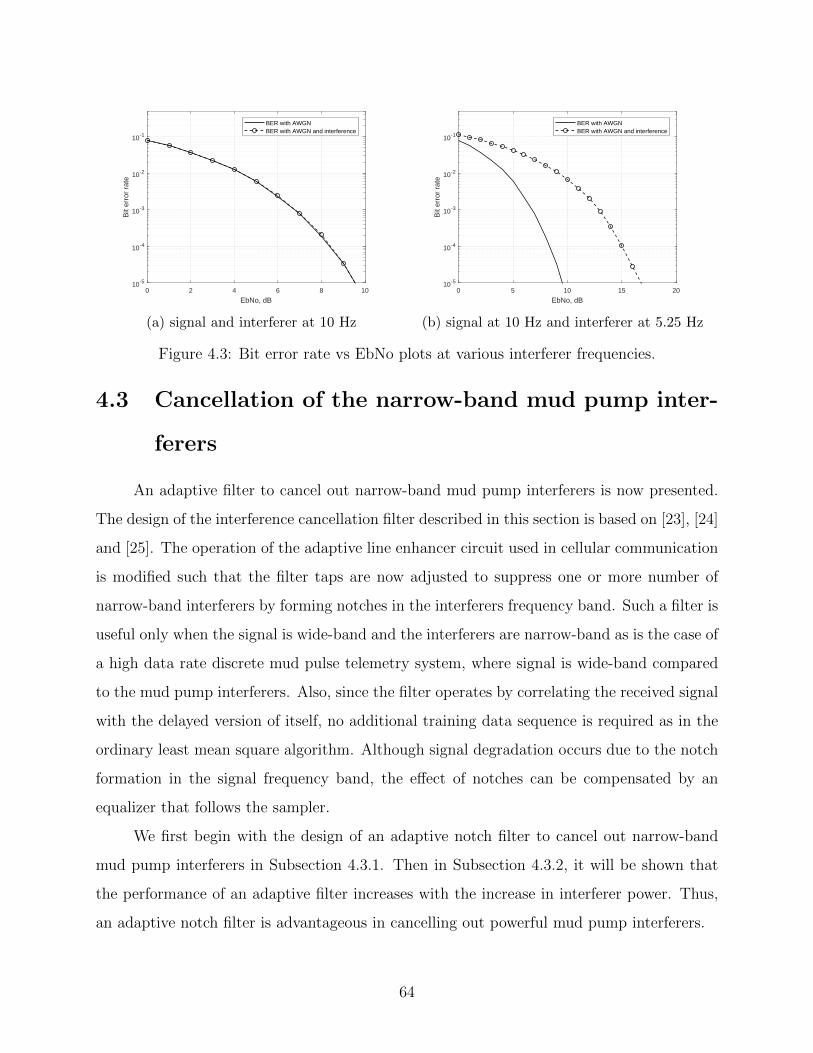
0 2 4 6 8 10

EbNo, dB

10-5

10-4

10-3

10-2

10-1

Bit

erro

r ra

teBER with AWGNBER with AWGN and interference

(a) signal and interferer at 10 Hz

0 5 10 15 20

EbNo, dB

10-5

10-4

10-3

10-2

10-1

Bit

erro

r ra

te

BER with AWGNBER with AWGN and interference

(b) signal at 10 Hz and interferer at 5.25 Hz

Figure 4.3: Bit error rate vs EbNo plots at various interferer frequencies.

4.3 Cancellation of the narrow-band mud pump inter-

ferers

An adaptive filter to cancel out narrow-band mud pump interferers is now presented.

The design of the interference cancellation filter described in this section is based on [23], [24]

and [25]. The operation of the adaptive line enhancer circuit used in cellular communication

is modified such that the filter taps are now adjusted to suppress one or more number of

narrow-band interferers by forming notches in the interferers frequency band. Such a filter is

useful only when the signal is wide-band and the interferers are narrow-band as is the case of

a high data rate discrete mud pulse telemetry system, where signal is wide-band compared

to the mud pump interferers. Also, since the filter operates by correlating the received signal

with the delayed version of itself, no additional training data sequence is required as in the

ordinary least mean square algorithm. Although signal degradation occurs due to the notch

formation in the signal frequency band, the effect of notches can be compensated by an

equalizer that follows the sampler.

We first begin with the design of an adaptive notch filter to cancel out narrow-band

mud pump interferers in Subsection 4.3.1. Then in Subsection 4.3.2, it will be shown that

the performance of an adaptive filter increases with the increase in interferer power. Thus,

an adaptive notch filter is advantageous in cancelling out powerful mud pump interferers.

64

4.3.1 Design of an adaptive notch filter

x(t) y(t)

i(t)

W0 W1 W2WL-1

z- z-1 z-1 z-1

+ _

received signalsignal andnoise

estimate ofinterference

Adaptive filter

˜

Figure 4.4: An adaptive notch filter for cancelling out narrow-band interferers.

The received signal at the output of mud channel as given in (4.2) can be written as

x(t) = s(t) + i(t) + n(t), (4.22)

where the channel impulse response, hc(t) = δ(t) is taken for convenience and i(t) is the

net interference as given in (4.10). Let σ2d denotes power of a desired signal s(t), σ2

in = a2n2

represents the power of the nth narrow-band interferer and σ2w is the variance of the white

noise.

Fig. 4.4 shows the structure of an adaptive notch filter. The objective is to design

a filter such that the narrow-band interferers are suppressed at the output, i.e. the filter

places notches at the interferers frequency band. This is possible by sufficiently delaying the

received signal x(t) by an amount ∆ so that the delayed signal samples of s(t+ ∆) and the

original signal samples of s(t) are approximately uncorrelated. Thus, the signal and noise

samples being wide-band are uncorrelated at the different filter taps, whereas the interferers

being narrow-band consist of correlated samples. The present sample of the interferers can

be predicted from their past samples, which when subtracted from the received input gives

an error output comprising of the desired signal and wide-band noise ideally. The error is

then used to adjust the filter weights such that the resulting mean-square error is minimized.

65

The received signal at sampling instant t = mT is given as

x(mT ) = s(mT ) +N∑n=1

ancos(ωnmT + θn) + n(mT ). (4.23)

The Wiener-Hopf solution for the optimum tap weights for the notch filter can be written as

L−1∑k=0

rxx(l − k)wopt(k) = rxx(l + ∆), l = 0, 1, · · ·L− 1. (4.24)

In (4.24), rxx(l − k) denotes the auto-correlation of the received signal x(mT ), rxx(l + ∆)

denotes the cross-correlation of the received signal x(mT ) with its own delayed version

x(mT + ∆) and wopt(k) represents the optimum tap weight. The auto-correlation function

of the received signal for a lag l can be written as

rxx(l) = (σ2d + σ2

w)δ(l) +N∑n=1

σ2in cos(lωn). (4.25)

The values of the optimum tap weights can be obtained by the method of undetermined

coefficients [23],[24],[25]. In this method, for the sinusoidal narrow-band signals in a wide-

band signal, the solution of wopt(k) is assumed in terms of unknown constants, which when

substituted in (4.24) give a set of equations for the unknown constants. The solution of the

tap weights for N input sinusoidal interferers can be written as [23]

wopt(k) =N∑n=1

An(ejkωn + e−jkωn), (4.26)

where An are the unknown coefficients to be determined.

Equation (4.26) is the general solution of optimum filter taps for N sinusoidal interferers.

For the convenience of computational simplicity, we derive the optimum filter taps of the

notch filter for N = 1. In this case,

wopt(k) = A1(ejkω1 + e−jkω1). (4.27)

66

For the solution of unknown A1, substituting (4.25) and (4.27) in lth equation of (4.24), we

getL−1∑k=0

{(σ2

d + σ2w)δ(l − k) + σ2

i cos(l − k)ω1

}A1(ejkω1 + e−jkω1)

= (σ2d + σ2

w)δ(l + ∆) + σ2i cos(l + ∆)ω1, (4.28)

where σ2i = σ2

i1=

a212

is the power of a single interferer. Further simplification of (4.28) yields

L−1∑k=0

A1(σ2d +σ2

w)ejkω1δ(l− k) +L−1∑k=0

A1(σ2d +σ2

w)e−jkω1δ(l− k) +L−1∑k=0

A1σ2i cos(l− k)ω1e

jkω1+

L−1∑k=0

A1σ2i cos(l − k)ω1e

−jkω1 = (σ2d + σ2

w)δ(l + ∆) + σ2i cos(l + ∆)ω1

or

A1(σ2d + σ2

w)ejlω1 + A1(σ2d + σ2

w)e−jlω1 +A1σ

2i

2

[L−1∑k=0

{ej(l−k)ω1 + e−j(l−k)ω1

}ejkω1

]

+A1σ2

i

2

[L−1∑k=0

{ej(l−k)ω1 + e−j(l−k)ω1

}e−jkω1

]= (σ2

d+σ2w)δ(l+∆)+

σ2i

2

[ej(l+∆)ω1 + e−j(l+∆)ω1

].

(4.29)

Comparing coefficients of ejlω1 (or e−jlω1) on both sides of (4.29) gives

A1(σ2d + σ2

w) +A1σ

2iL

2+A1σ

2i

2

L−1∑k=0

e−2jkω1 =σ2i

2ej∆ω1 (4.30)

or

A1 =σ2i ej∆ω1

2(σ2d + σ2

w) + σ2iL+ σ2

i

L−1∑k=0

e−2jkω1

. (4.31)

Equivalently,

A1 =σ2i ej∆ω1

2(σ2d + σ2

w) + σ2iL+ σ2

isin(Lω1)sin(ω1)

e−j(L−1)ω1

. (4.32)

The estimate of the spectrum of the interferers, which is given by the transfer function of

67

adaptive filter is then given as

H(ω) =L−1∑k=0

wopt(k)e−jωk

or

H(ω) =L−1∑k=0

A1

[ejkω1 + e−jkω1

]e−jωk. (4.33)

Substituting the value of A1 in (4.33) we get

H(ω) =σ2i ej∆ω1

[L−1∑k=0

ej(ω1−ω)k+L−1∑k=0

e−j(ω1+ω)k

]

2(σ2d + σ2

w) + σ2iL+ σ2

isin(Lω1)sin(ω1)

e−j(L−1)ω1

or

H(ω) =σ2i ej∆ω1

[sin{(ω1−ω)L2 }sin{(ω1−ω) 12}

ej2 (ω1−ω)(L−1)+

sin{(ω1+ω)L2 }sin{(ω1+ω) 12}

e−j2 (ω1+ω)(L−1)

]

2(σ2d + σ2

w) + σ2iL+ σ2

isin(Lω1)sin(ω1)

e−j(L−1)ω1

. (4.34)

As shown in Fig. 4.4, the estimate of the interferers is now subtracted from the received

signal resulting in the estimate of the desired signal and the wide-band noise. Once the

estimate of interferers is known, the frequency response of a notch filter Hsf (ω) can be

obtained as

Hsf (ω) = 1−H∗(ω), (4.35)

where H∗(ω) denotes complex conjugate of H(ω).

As an example plot, Fig. 4.5 shows the spectrum of a single sinusoid at 5.25 Hz

(32.96 rad/sec) and response of an adaptive notch filter forming a notch at the frequency

of an interfering sinusoid. The plot is generated using (4.34) and (4.35), where the signal,

interference and noise are assumed to have unit power each. The received signal is delayed

by the time equal to twice the signal duration to ensure that the desired signal at each filter

taps are approximately uncorrelated. The total number of filter taps for this plot is 101.

68

32.6 32.8 33 33.2 33.4 33.6

Angular frequency ( )

-0.2

0

0.2

0.4

0.6

0.8

1

1.2

1.4A

mpl

itude

Spectrum of a sinusoidal interferenceResponse of an adaptive notch filter

Figure 4.5: Frequency response of a notch filter for a single interferer at 32.96 rad/sec.

4.3.2 Performance of an adaptive notch filter

The minimum mean-square error at the output of a notch filter shown in Fig. 4.1 at a

time t = mT is given as [25]

E[y2m]min = rxx(0)−

L∑k=1

rxx(k)wopt(k), (4.36)

where y(mT ) is denoted by ym for simplicity. Substituting the values of rxx(0), rxx(k) and

wopt(k) from (4.25) and (4.27) in (4.36) for a single interferer, we get

E[y2m]min = σ2

d + σ2w + σ2

i −L∑k=1

[(σ2

d + σ2w)δ(k) + σ2

i cos(kω1)]A1(ejω1k + e−jω1k), (4.37)

where the value of A1 is obtained from (4.32). The minimum mean-square error at the

output of a notch filter represents the power of the signal and noise. Thus, (4.36) can also

69

be written as

E[y2m]min = σ2

d + E[n2m], (4.38)

where E[n2m] represents the noise power of a sample at the output of a notch filter which is

the combined power of the wide-band channel noise and the residual interferers. Substituting

(4.38) in (4.37) and using relation δ(k) = 0, k 6= 0, we get

E[n2m] = σ2

i + σ2w − 2σ2

iA1

L∑k=1

cos2(kω1)

= σ2i + σ2

w −A1σ

2i

2

[2L+

L∑k=1

e2jkω1 +L∑k=1

e−2jkω1

]

= σ2i + σ2

w −A1σ

2i

2

[2L− 1 +

sin{(2L + 1)ω1}sin(ω1)

]. (4.39)

Now, the improvement in SINR due to the notch filter can be shown by considering

SINR at the input and output of a notch filter. The SINR at the input of a notch filter is

given as

SINRin =σ2d

σ2i + σ2

w

. (4.40)

The SINR at the output of a notch filter is given as

SINRout =σ2d

E[n2m]. (4.41)

The improvement in the SINR is then given as

γ =SINRout

SINRin

=σ2i + σ2

w

σ2i + σ2

w −A1σ2

i

2

[2L− 1 + sin{(2L+1)ω1}

sin(ω1)

] . (4.42)

Substituting the magnitude of A1 from (4.32) in (4.42), we get

γ =σ2i + σ2

w

σ2i + σ2

w −σ4i

4(σ2d+σ2

w)+2σ2i L+2σ2

isin(Lω1)sin(ω1)

e−j(L−1)ω1

[2L− 1 + sin{(2L+1)ω1}

sin(ω1)

] . (4.43)

70

To better understand the effect of the interferer to signal power ratio in the performance

improvement, lets assume σ2w = 0. Then (4.43) becomes

γ =1

1− 14J

+2L+2sin(Lω1)sin(ω1)

e−j(L−1)ω1

[2L− 1 + sin{(2L+1)ω1}

sin(ω1)

] . (4.44)

where, J =σ2i

σ2d

is the ratio of interferer power to the signal power. Equation (4.44) shows

that, higher the interference-to-signal power ratio, higher is the performance improvement

with the use of a notch filter.

0 5 10 15 20 25 30

J (dB)

14.5

15

15.5

16

16.5

17

(dB

)

Figure 4.6: Performance improvement by a notch filter with different interferer to signalpower ratios.

Fig. 4.6 shows the plot of (4.44), where the frequency of an interferer is set to 5.25 Hz.

The total number of filter taps, L is 101. It can be seen from the plot that as the ratio of

the interferer to signal power, J increases, the improvement in the performance, γ increases.

Thus, a notch filter is suitable for cancelling out the narrow-band interferers from the mud

pump, where the sinusoidal interferers have higher power compared to the desired wide-band

signal.

71

4.4 Channel Equalization

Channel equalization is the process of compensating the effect of the channel distortion.

An equalizer is used as a linear filter to minimize the effect of ISI at the output of the

receiver. A much simpler approach of obtaining no ISI condition at the output of a receiver

is by modelling an equalizer as an inverse of the channel impulse response. This is the

principle used in zero-forcing equalizers. However, the major drawback of this approach is the

severe noise enhancement. Since the mud channel impulse response exhibits nulls and higher

attenuation at upper frequencies, simply inverting the channel response tends to supply

high gain at such frequency regions leading to noise enhancement. Thus, there is always

a compromise between the noise enhancement and channel equalization. A good balance

between these two parameters can be achieved in minimum mean-square error equalizers

(MMSE). In these equalizers, the mean-square error between the desired response and the

filter output is taken as the cost function and an attempt is made to minimize this error

while taking care of noise exaggeration problem.

MMSE equalizers are commonly implemented as Weiner filters. The theory of Weiner

filter is summarized in Subsection 4.4.1. An optimum solution of Weiner filter taps can also

be obtained from LMS algorithm. Basic steps for LMS algorithm are briefed in Subsection

4.4.2.

4.4.1 Wiener filters

+ + +z(k)

z-1r(k) r(k-1) r(k-M+2) r(k-M+1)

z-1 z-1

c0c1

cM-1CM-2

Figure 4.7: Weiner filter as a tapped-delay line.

According to the Wiener filter theory, a linear filter can be assumed as a discrete time

72

tapped-delay line [44]. The output of the filter as shown in (4.9) at any discrete time k is

z(k), where the notation k is used hereafter to represent the sampled signal at time kT .

The delay τ0 is simply omitted for simplicity. This output acts as an estimate of the desired

response. The estimation error at time k, e(k), is defined as the difference between the

desired response s(k) and the estimate of the desired response z(k). This error is inevitable

as both the input to the filter and the desired response are taken as a single realization of

a wide sense stationary random process. The requirement of the Weiner filter is to find the

optimum filter weights such that mean-square value of e(k) is minimum.

As shown in Fig. 4.7, for a filter of order M, let r(k) represents an M × 1 tap input

vector which is the vector of discrete samples at the input of an equalizer as given in Fig. 4.1.

Then, the matrix E[rT (k)r(k)] denotes the auto-correlation matrix between the tap input

vector to the filter. Denoting the auto-correlation matrix by R, the M ×M matrix has the

following structure

R =

E[r2(k)] E[r(k)r(k − 1)] . . . E[r(k)r(k −M + 1)]

E[r(k − 1)r(k)] E[r2(k − 1)] . . . E[r(k − 1)r(k −M + 1)]

. . . . . . . . . . . .

E[r(k −M + 1)r(k)] E[r(k −M + 1)r(k − 1)] . . . E[r2(k −M + 1)]

.(4.45)

For a real zero mean wide stationary random process, the auto-correlation matrix is a sym-

metric Toeplitz matrix. The wide sense stationary nature of random process also implies

that the auto-correlation matrix is an even function independent of the time shift. The nth

entry of a matrix R is given as

arr(n) = E[r(k)r(k + n)]

and

arr(−n) = arr(n).

73

Thus, the matrix R can be written in an expanded form as

R =

arr(0) arr(1) . . . arr(M − 1)

arr(1) arr(0) . . . arr(M − 2)

. . . . . . . . . . . .

arr(M − 1) arr(M − 2) . . . arr(0)

. (4.46)

Similarly, the vector E[r(k)s(k)] denotes the cross-correlation between the tap input vector

and the desired response. Denoting the cross-correlation vector by P, the M × 1 vector has

following structure

P =

E[r(k)s(k)]

E[r(k − 1)s(k)]

. . .

E[r(k −M + 1)s(k)]

. (4.47)

The cross-correlation vector is also independent of time and thus can also be written in the

form

P =

p(0)

p(1)

. . .

p(M − 1)

. (4.48)

Now, for a given value of R and P the Weiner filter problem is to find the optimum values of

tap vector c such that the mean square value of the error is minimum. The optimum value

of the tap vector is given by Weiner-Hopf equation [44] as

copt = R−1P. (4.49)

4.4.2 LMS algorithm

The implementation of the Weiner-Hopf equation to determine the optimum filter

weights requires the knowledge of the auto-correlation matrix R and the cross-correlation

vector P. Furthermore, the optimum solution exists only if the matrix R is non singular.

74

Another method of determining the optimum filter weights without explicitly computing R

and P is by the method of steepest gradient algorithm. An stochastic gradient algorithm

assumes that the optimal solution to the weight vector exists. Since the mean-square error

given by the Weiner filter is quadratic in nature, the error performance has a unique minimum

and hence, the optimum weight vector exists.

LMS algorithm is an example of an stochastic gradient algorithm. The algorithm is

iterative in nature, i.e. it starts from any arbitrary value of a tap weight vector and with each

iteration, the weights are updated. The final weight vector converges to the Weiner-Hopf

solution given by (4.49). The LMS algorithm can be summarized as follows [44].

1. Start with an arbitrary value c(n-1) of the tap weight vector c of size M × 1 at time

t = n− 1. This arbitrary vector serves as an initial guess of the optimum tap weights.

2. Form an input vector of equalizer input r(n), n = 1, 2, . . . , N of size M × 1, where N is

the total number of signal samples input to an equalizer.

3. For each sample of the equalizer input r(n), the equalizer output at time n is computed

as

z(n) = cT (n− 1)r(n)

. 4. The error e(n) is then given as

e(n) = s(n)− z(n)

where, s(n) is the desired signal sample at the time instant n.

5. The tap coefficients of the equalizer at the instant n are updated as

c(n) = c(n− 1) + ∆r(n)e(n)

, where ∆ is the step size of the LMS algorithm. It controls the incremental correction of the

weight vector and plays an important role in the speed of convergence of the LMS algorithm

[44]. Generally, a small value of ∆ gives a lower minimum mean-square error. This however

comes at the cost of the increased run time of the algorithm. The value of ∆ is typically

75

selected as [46]

0 < ∆ <1

10MPx, (4.50)

where M is the size of adaptive filter and Px is the power of input signal.

6. Go to step 2 and terminate when n = N .

When the tap coefficients attain the optimum values, copt obtained from the LMS algorithm

converges to the optimum values of the tap coefficients obtained from the Weiner-Hopf

solution.

76

Chapter 5

Simulation results

This chapter provides simulation results to verify the theories developed in the pre-

ceding chapters. Base-band discrete pressure pulses at 10 bps and 20 bps are considered for

the simulations. Section 5.1 tabulates mud, drill pipe and mud pump parameters that are

used in the simulations. The presented data are chosen to match closely with the actual

parameters used in the industry. Section 5.2 presents the attenuation behaviour of the mud

pulse at different data rates based on the fluid transmission line model. In Section 5.3, the

mud channel transfer function obtained from the fluid transmission line is verified with an

equivalent electrical transmission line circuit in ADS and the corresponding impulse response

functions are plotted. Finally, in Section 5.4, the designed receiver is tested to equalize the

mud channel and cancel out the narrow-band interferers. The performance of the equalizer

and notch filter are measured in terms of bit error rates and packet error rates.

5.1 Simulation parameters

As described in the preceding chapters, the attenuation characteristics and the transfer

function of the mud channel derived from the fluid transmission line depend on the proper-

ties of the mud, physical dimension of the drill pipe and junction as well as on the distance

of pressure transducer from the mud pump. The interferers on the other hand being orig-

inated from the mud pump depend on the characteristics of the mud pump used. Thus,

information regarding the properties of the mud, the dimension of drill pipe and junction,

77

the characteristics of the mud pump used and the distance of pressure sensor from the mud

pump are given next.

For the simulations, water-based mud from [17] is considered. The various properties

of the mud along with their SI units are listed in Table 5.1.

Mud properties ValuesDensity(ρ), kgm−3 1066.5Dynamic viscosity(η), kgm−1s−1 1.9× 10−2

Kinematic viscosity(v), m2s−1 1.78× 10−5

Bulk modulus(B), Pa 2.39× 109

Table 5.1: Drilling mud parameters.

A frequently used IEU S135 drill pipe is considered for the simulations. The drill pipe

is made up of 42CrMo material. The details of the drill pipe as described in [51] and [52]

are given in Table 5.2. With the available data, the geometry of the drill pipe including the

Drill pipe and junction properties ValuesYoungs modulus(E), Pa 2.07× 1011

Poisson ratio(λ) 0.29Length of each pipe section (lp), m 9.144Pipe outer diameter (ap), m 0.254Pipe inner diameter (bp), m 0.2172Length of each junction section (lj), m 0.1524Junction outer diameter (aj), m 0.336Junction inner diameter (bj), m 0.181

Table 5.2: Drill pipe and junction parameters.

transition area and junction is shown in Fig. 5.1. The pressure transducer is considered to

0.254 0.2172 0.336 0.181

9.144 0.1524 9.144

Figure 5.1: Geometry of the drill pipe with junction.

be located at a distance of 15.24 m from the mud pump [48].

78

National Oilwell Varco’s 14-P-220 triplex mud pump described in Chapter 2 is consid-

ered for the simulation. It has a maximum rated input of 2200 HP at 105 strokes per minute

and is capable of maintaining maximum volumetric flow rate of 1215 gpm. The specifications

of the mud pump from [61] are summarized in Table 5.3.

Mud pump specifications ValuesNumber of pistons 3Pump action 1Stroke rate (strokes/min) 105

Table 5.3: A 14-P-220 triplex mud pump parameters.

5.2 Attenuation of the pressure pulses at different data

rates

Using the data from Table 5.1 and Table 5.2, the values of R, L, C and α for the pipe

and junction sections are obtained using (3.3),(3.5),(3.9) and (3.36) respectively, as given

in Chapter 3. Then, (3.46) is applied to obtain the amplitude of the attenuated pressure

pulses received by the pressure sensor from different depths. As stated earlier, the pressure

pulses are assumed to be discrete base-band square pulse signals. A base-band square pulse

has a sinc2 power spectrum centred around 0 Hz with an infinite bandwidth. However, as

maximum energy of the spectrum is concentrated in the main lobe of a sinc2 spectrum, the

truncated spectrum with one sided bandwidth of 10 Hz and 20 Hz are considered for 10 bps

and 20 bps square pulses respectively. It means that substituting the value of the frequency

as 10 Hz or 20 Hz in (3.36) approximates the attenuation per unit length for 10 bps or 20

bps square pulse respectively. The amplitude versus depth plot of 100 kpa pressure wave at

10 and 20 bps is shown Fig. 5.2.

The plot in Fig. 5.2 verifies the exponential decay nature of the pressure pulses as a

function of the well depth and the fact that a 20 bps pressure pulse attenuates rapidly as

compared to a 10 bps pressure pulse.

79

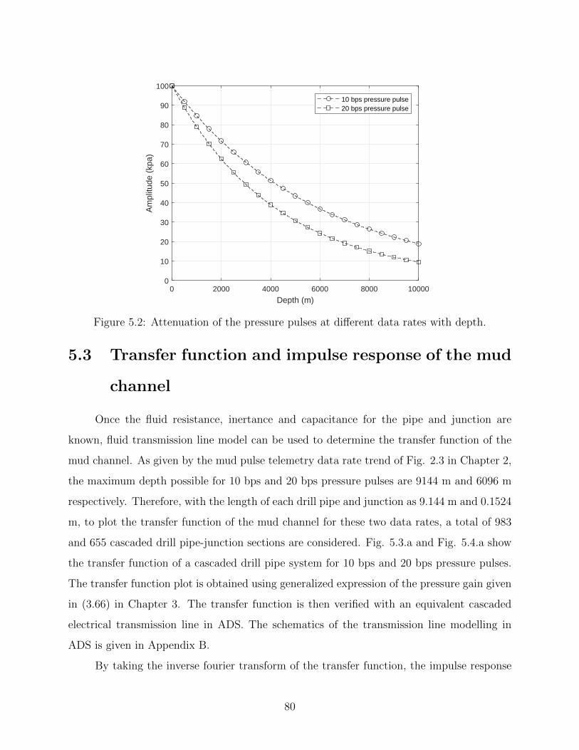
0 2000 4000 6000 8000 10000

Depth (m)

0

10

20

30

40

50

60

70

80

90

100

Am

plitu

de (

kpa)

10 bps pressure pulse20 bps pressure pulse

Figure 5.2: Attenuation of the pressure pulses at different data rates with depth.

5.3 Transfer function and impulse response of the mud

channel

Once the fluid resistance, inertance and capacitance for the pipe and junction are

known, fluid transmission line model can be used to determine the transfer function of the

mud channel. As given by the mud pulse telemetry data rate trend of Fig. 2.3 in Chapter 2,

the maximum depth possible for 10 bps and 20 bps pressure pulses are 9144 m and 6096 m

respectively. Therefore, with the length of each drill pipe and junction as 9.144 m and 0.1524

m, to plot the transfer function of the mud channel for these two data rates, a total of 983

and 655 cascaded drill pipe-junction sections are considered. Fig. 5.3.a and Fig. 5.4.a show

the transfer function of a cascaded drill pipe system for 10 bps and 20 bps pressure pulses.

The transfer function plot is obtained using generalized expression of the pressure gain given

in (3.66) in Chapter 3. The transfer function is then verified with an equivalent cascaded

electrical transmission line in ADS. The schematics of the transmission line modelling in

ADS is given in Appendix B.

By taking the inverse fourier transform of the transfer function, the impulse response

80

of the mud channel is obtained. In simulations, the continuous time base-band square pulse,

noise and interferers from the mud pump are approximated with their discrete forms sampled

at 100 Hz, therefore, the channel is also sampled at 100 Hz. The truncated impulse response

of the mud channel for 10 bps and 20 bps pressure pulses are shown in Fig. 5.3.b and Fig.

5.4.b respectively.

0 10 20 30 40 50 60 70 80 90 100

Frequency(Hz)

-120

-100

-80

-60

-40

-20

0

Mag

nitu

de(d

B)

Matlab plotADS plot

(a) Transfer function of mud channel.

6 6.5 7 7.5 8

Time(sec)

0

0.01

0.02

0.03

0.04

0.05

0.06

0.07

0.08

0.09

Am

plitu

de

(b) Impulse response of mud channel.

Figure 5.3: Transfer function and impulse response of a 9144 m deep mud channel (for 10bps pressure pulse).

0 10 20 30 40 50 60 70 80 90 100

Frequency(Hz)

-80

-70

-60

-50

-40

-30

-20

-10

0

Mag

nitu

de(d

B)

Matlab plotADS plot

(a) Transfer function of mud channel.

4.2 4.4 4.6 4.8 5 5.2

Time(sec)

0

0.02

0.04

0.06

0.08

0.1

0.12

0.14

0.16

Am

plitu

de

(b) Impulse response of mud channel.

Figure 5.4: Transfer function and impulse response of a 6096 m deep mud channel (for 20bps pressure pulse).

Fig. 5.3.a and Fig. 5.4.a show the frequency selective nature of a mud channel. The

channel gain of the mud channel with a total depth of 6096 m is higher than the channel

gain of the mud channel with a total depth of 9144 m due to the smaller overall depth of the

81

pressure wave propagation. At higher frequencies, fluid resistance increases. This increases

the attenuation of the pressure pulses and hence the channel gain in both cases decreases,

resulting in the severe amplitude distortion of the pressure pulses.

As shown by (3.67) in Chapter 3, with the pressure transducer at a distance of 15.24 m

from mud pump and pressure wave velocity at the pipe to be 1307 ms−1, nulls in the transfer

function of Fig. 5.3.a and Fig. 5.4.a occur at 21.4 Hz, 64.2 Hz and so on. Due to the cascade

of pipe and junctions, the effect of reflections from the junctions causes notch at 70.2 Hz.

It is also to be noted that the location of nulls for both 9144 m and 6096 m deep pressure

pulse channel in Fig. 5.3.a and Fig. 5.4.a are same. It is because, the locations of the nulls

given by (3.67) do not depend on the depth of the mud channel but only depend on the

location of the pressure sensor from the mud pump. A sinusoidal modulated pressure wave

with a frequency matching with the frequency of nulls or notches may result in complete

destruction of the transmitted pressure wave signal.

0 10 20 30 40 50 60 70 80 90 100

Frequency(Hz)

-80

-70

-60

-50

-40

-30

-20

-10

0

Mag

nitu

de(d

B)

Matlab plotADS plot

(a) Transducer at a distance of 30.48 m.

0 10 20 30 40 50 60 70 80 90 100

Frequency(Hz)

-70

-60

-50

-40

-30

-20

-10

0

Mag

nitu

de(d

B)

Matlab plotADS plot

(b) transducer at distance of 152.4 m.

Figure 5.5: Transfer function of a 9144 m deep mud channel with varying distance of pressuretransducer from the mud pump.

The effect of changing the transducer location on the channel transfer function is shown

in Fig. 5.5.a and Fig. 5.5.b. For simplicity, the transfer function corresponding to 10 bps

pressure pulse is shown and the case with 20 bps can be analysed accordingly. Comparing

Fig. 5.3.a with Fig. 5.5.a and Fig. 5.5.b it is seen that the nulls appear frequently in the

transfer function when the transducer location is moved away from the mud pump which

decrease the coherent bandwidth of the mud channel. Such nulls have adverse effect on the

82

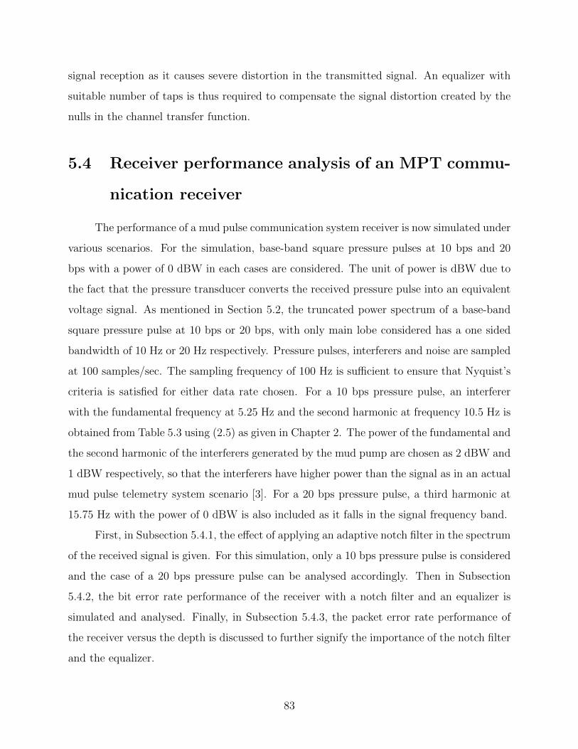
signal reception as it causes severe distortion in the transmitted signal. An equalizer with

suitable number of taps is thus required to compensate the signal distortion created by the

nulls in the channel transfer function.

5.4 Receiver performance analysis of an MPT commu-

nication receiver

The performance of a mud pulse communication system receiver is now simulated under

various scenarios. For the simulation, base-band square pressure pulses at 10 bps and 20

bps with a power of 0 dBW in each cases are considered. The unit of power is dBW due to

the fact that the pressure transducer converts the received pressure pulse into an equivalent

voltage signal. As mentioned in Section 5.2, the truncated power spectrum of a base-band

square pressure pulse at 10 bps or 20 bps, with only main lobe considered has a one sided

bandwidth of 10 Hz or 20 Hz respectively. Pressure pulses, interferers and noise are sampled

at 100 samples/sec. The sampling frequency of 100 Hz is sufficient to ensure that Nyquist’s

criteria is satisfied for either data rate chosen. For a 10 bps pressure pulse, an interferer

with the fundamental frequency at 5.25 Hz and the second harmonic at frequency 10.5 Hz is

obtained from Table 5.3 using (2.5) as given in Chapter 2. The power of the fundamental and

the second harmonic of the interferers generated by the mud pump are chosen as 2 dBW and

1 dBW respectively, so that the interferers have higher power than the signal as in an actual

mud pulse telemetry system scenario [3]. For a 20 bps pressure pulse, a third harmonic at

15.75 Hz with the power of 0 dBW is also included as it falls in the signal frequency band.

First, in Subsection 5.4.1, the effect of applying an adaptive notch filter in the spectrum

of the received signal is given. For this simulation, only a 10 bps pressure pulse is considered

and the case of a 20 bps pressure pulse can be analysed accordingly. Then in Subsection

5.4.2, the bit error rate performance of the receiver with a notch filter and an equalizer is

simulated and analysed. Finally, in Subsection 5.4.3, the packet error rate performance of

the receiver versus the depth is discussed to further signify the importance of the notch filter

and the equalizer.

83

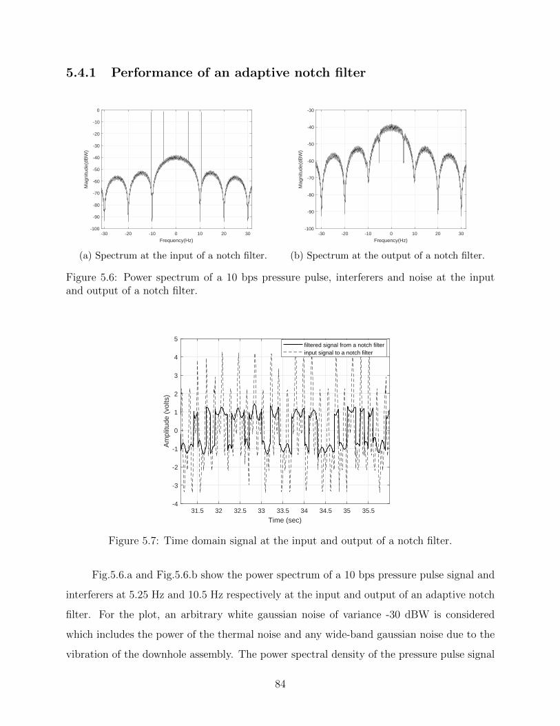
5.4.1 Performance of an adaptive notch filter

-30 -20 -10 0 10 20 30

Frequency(Hz)

-100

-90

-80

-70

-60

-50

-40

-30

-20

-10

0

Mag

nitu

de(d

BW

)

(a) Spectrum at the input of a notch filter.

-30 -20 -10 0 10 20 30

Frequency(Hz)

-100

-90

-80

-70

-60

-50

-40

-30

Mag

nitu

de(d

BW

)

(b) Spectrum at the output of a notch filter.

Figure 5.6: Power spectrum of a 10 bps pressure pulse, interferers and noise at the inputand output of a notch filter.

31.5 32 32.5 33 33.5 34 34.5 35 35.5

Time (sec)

-4

-3

-2

-1

0

1

2

3

4

5

Am

plitu

de (

volts

)

filtered signal from a notch filterinput signal to a notch filter

Figure 5.7: Time domain signal at the input and output of a notch filter.

Fig.5.6.a and Fig.5.6.b show the power spectrum of a 10 bps pressure pulse signal and

interferers at 5.25 Hz and 10.5 Hz respectively at the input and output of an adaptive notch

filter. For the plot, an arbitrary white gaussian noise of variance -30 dBW is considered

which includes the power of the thermal noise and any wide-band gaussian noise due to the

vibration of the downhole assembly. The power spectral density of the pressure pulse signal

84

follows sinc2 function . The spikes at 5.25 Hz and 10.5 Hz in Fig. 5.6.a are the power spectral

densities of the random sinusoids generated from the mud pump. A notch filter discussed in

Section 4.3.1 in Chapter 4 is used and has a total 1001 taps. The large number of taps is

due to the fact that the notch filter is implemented before the matched filter as discussed in

Chapter 4. The received signal is delayed by a time period equal to twice the signal period

and is applied to the notch filter to ensure that the signal samples at the different filter taps

are approximately uncorrelated. The step size of the LMS algorithm used by the filter is

chosen according to (4.50) given in Chapter 4. The power spectral density at the output of

the notch filter in Fig. 5.6.b shows interferer free signal and noise spectrum with notches at

5.25 Hz and 10.5 Hz formed by the notch filter. The time domain filtered signal from the

notch filter is shown in Fig. 5.7.

5.4.2 Bit error rate performance of a mud pulse communication

system receiver under various scenarios

The bit error rate performance of a mud pulse communication system receiver is now

simulated. The simulation is performed under two scenarios. First, a 10 bps pressure pulse is

considered. For this case, the impulse response of the channel shown in Fig. 5.3.b distorts the

pressure pulses. Random sinusoids at 5.25 Hz and 10.5 Hz generated from the mud pump act

as narrow-band interferers along with the additive gaussian noise. The information regarding

the sampling frequency, power of the signal and interferers are given in Section 5.4.

Next, a 20 bps pressure pulse with an impulse response of the channel shown in Fig.

5.4.b is considered. In this case, a third interferer at 15.75 Hz is also considered as it falls

within the signal frequency band.

For the above two scenarios, an adaptive notch filter described in Subsection 5.4.1 is

used. The output of the filter undergoes matched filtering, which is sampled every symbol

time and the output is applied to a Weiner filter described in Subsection 4.4.1 in Chapter 4

with the tap size twice the size of the channel. An LMS algorithm discussed in Subsection

4.4.2 in Chapter 4 can also be used as an equalizer when the channel is considerably long.

As the significant taps of the channel impulse response, shown in Fig. 5.3.b and Fig. 5.4.b,

85

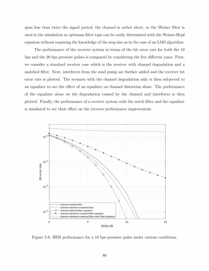
span less than twice the signal period, the channel is rather short, so the Weiner filter is

used in the simulation as optimum filter taps can be easily determined with the Weiner-Hopf

equation without requiring the knowledge of the step size as in the case of an LMS algorithm.

The performance of the receiver system in terms of the bit error rate for both the 10

bps and the 20 bps pressure pulses is compared by considering the five different cases. First,

we consider a standard receiver case which is the receiver with channel degradation and a

matched filter. Next, interferers from the mud pump are further added and the receiver bit

error rate is plotted. The scenario with the channel degradation only is then subjected to

an equalizer to see the effect of an equalizer on channel distortion alone. The performance

of the equalizer alone on the degradation caused by the channel and interferers is then

plotted. Finally, the performance of a receiver system with the notch filter and the equalizer

is simulated to see their effect on the receiver performance improvement.

0 5 10 15

EbNo,dB

10-4

10-3

10-2

10-1

Bit

erro

r ra

te

channel+matched filterchannel+interferers+matched filterchannel+matched filter+equalizerchannel+interferers+matched filter+equalizerchannel+interferers+matched filter+notch filter+equalizer

Figure 5.8: BER performance for a 10 bps pressure pulse under various conditions.

86

Fig. 5.8 shows the above five scenarios for a 10 bps pressure pulse. The BER degrada-

tion due to the channel distortion alone for a 10 bps is less severe. This is evident from the

channel impulse response for a 10 bps pressure pulse shown in Fig. 5.3.b. As the pressure

pulse has a time period of 0.1 sec, the delay spread of the channel is nearly within the signal

period. This results is the lesser ISI. As a result, the effect of the channel is not harsh.

As the interferers at 5.25 Hz and 10.5 Hz do not fall at the integral multiples of the signal

frequency, from Section 4.2 in Chapter 4, we expect the adverse effect of the interferers on

the bit error rate. This is clearly shown by Fig. 5.8, where the receiver with the channel

and the interferers acting together has the highest bit error rate. Applying an equalizer

to compensate the effect of the channel distortion alone provides the least bit error rate.

However, when the interferers are present, applying an equalizer alone does not seem much

useful to improve the bit error rate. The equalizer in this case, compensates the channel

distortion, however, fails to remove the effect of the interferers on the signal distortion. This

degradation of the receiver performance can be much improved by using a notch filter to

cancel out the narrow-band interferers followed by an equalizer to compensate the channel

distortion as shown by the improvement in the bit error rate. As described in Subsection

5.4.1, the use of a notch filter to remove the narrow-band interferers creates notches in the

signal frequency band. This causes slight distortion of the useful signal and hence contributes

to the bit error rate degradation. This explains the degradation of the bit error rate using

a notch filter and an equalizer in Fig. 5.8 as compared to the performance of the receiver

system using an equalizer to compensate the effect of the channel degradation only. Finally,

referring to Fig. 5.8, at an EbNo ratio of 5 dB, the use of a notch filter and an equalizer

leads to a reduction of bit error rate by nearly 10 times as compared to the case when no

notch filter and equalizer are used in the receiver system. The BER performance is further

improved for higher EbNo ratios. Thus, the application of the notch filter and an equalizer

in receiver performance improvement is justified.

Fig. 5.9 describes the same five scenarios for a 20 bps pressure pulse. In this case,

the severe effect of the channel is clearly represented by the bit error rate curve due to

the channel distortion alone. The severe effect of the channel is evident from the impulse

response for a 20 bps mud channel shown by Fig. 5.4.b, where the delay spread of the signal

87

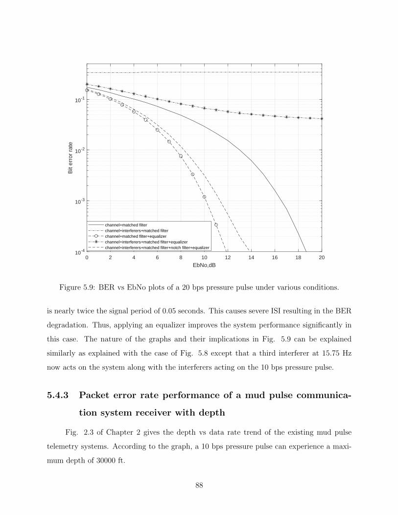
0 2 4 6 8 10 12 14 16 18 20

EbNo,dB

10-4

10-3

10-2

10-1

Bit

erro

r ra

te

channel+matched filterchannel+interferers+matched filterchannel+matched filter+equalizerchannel+interferers+matched filter+equalizerchannel+interferers+matched filter+notch filter+equalizer

Figure 5.9: BER vs EbNo plots of a 20 bps pressure pulse under various conditions.

is nearly twice the signal period of 0.05 seconds. This causes severe ISI resulting in the BER

degradation. Thus, applying an equalizer improves the system performance significantly in

this case. The nature of the graphs and their implications in Fig. 5.9 can be explained

similarly as explained with the case of Fig. 5.8 except that a third interferer at 15.75 Hz

now acts on the system along with the interferers acting on the 10 bps pressure pulse.

5.4.3 Packet error rate performance of a mud pulse communica-

tion system receiver with depth

Fig. 2.3 of Chapter 2 gives the depth vs data rate trend of the existing mud pulse

telemetry systems. According to the graph, a 10 bps pressure pulse can experience a maxi-

mum depth of 30000 ft.

88

The packet error rate is related to the bit error rate as

PER = 1− (1− BER)n, (5.1)

where n is the number of bits per packet.

Consider an arbitrary packet with the total number of bits as 96. Assuming the receiver

performance with the channel degradation and the matched filter only of Fig. 5.8 as the

standard receiver performance, for 96 bits per packet, we first set threshold packet error rate

as 90 %, i.e. the standard receiver stops working when the PER exceeds 0.90. This PER

corresponds to the 30000 ft depth. Now, the PER of 90% corresponds to the 5 dB EbNo

ratio from the BER curve of standard receiver performance as given in Fig. 5.8. With this

EbNo value corresponding to the 30000 ft, and for the given signal energy, we find the noise

level. This noise level is set as the constant noise level for all depths. Furthermore, for a unit

amplitude 10 bps pressure pulse and the EbNo ratio of 5 dB, the noise level turns out to

be much higher than the noise level considering the thermal noise alone. This means that,

the calculated constant noise level includes the gaussian noise from additional sources such

as downhole vibrations besides the thermal noise. As the depth decreases, the channel gain

increases and hence, the receiver performs better. With the fixed noise level corresponding

to 30000 ft, we find the BER and correspondingly the PER using (5.1), at various depths.

Using this information, the depth vs PER plots of the five scenarios discussed in Subsection

5.4.2 are given in Fig. 5.10.

The trend of the PER performance improvement under various scenarios shown by the

Fig. 5.10 follows the same pattern as explained with Fig. 5.8 and Fig. 5.9. Furthermore,

it is seen from the graph that the addition of interferers to the standard receiver reduces

its depth capability from 30000 ft to 21000 ft. Using a notch filter and an equalizer to the

cancel out the narrow-band interferers and compensate the channel distortion gives a total

depth capability of 33000 ft to the mud pulse receiver, a total gain of 12000 ft as compared

to the receiver with the channel distortion and the mud pump interferers.

89

900 3000 6000 9000 12000 15000 18000 21000 24000 27000 30000 33000 36000

Depth(ft)

0

0.1

0.2

0.3

0.4

0.5

0.6

0.7

0.8

0.9

1

Pac

ket e

rror

rat

e

channel+matched filterchannel+interferers+matched filterchannel+matched filter+equalizerchannel+interferers+matched filter+equalizerchannel+interferers+matched filter+notch filter+equalizer

Figure 5.10: Depth vs packet error rate performance of the mud pulse receiver for a 10 bpspressure pulse under various scenarios.

90

Chapter 6

Conclusion and future works

6.1 Conclusion

This research helps to understand the behaviour of the communication channel of a

mud pulse telemetry system and thus makes it easier to develop efficient receivers to achieve

the minimum bit error rate. By introducing a fluid transmission line model with lumped

components such as fluid resistance, inertance and capacitance, the dynamic properties of

the mud are easily coupled with the geometry of the drill pipe. This makes it possible

to obtain the attenuation characteristics of the pressure waves in an analogous way to an

electrical transmission line. The attenuation characteristics obtained from the developed

fluid transmission line model have been shown to match very closely with the attenuation

characteristics from the experimentally verified Lamb’s law of pressure wave attenuation

present in the existing literature for different frequencies. Further, the fluid transmission line

model is extended to represent the cascaded system of drill pipes including the mud pump

and the pressure transducer. The cascaded system of drill pipes gives a clear representation

of the pressure pulse reflection phenomenon from the junction connecting two drill pipes.

Thus, a frequency selective transfer function of the mud channel demonstrating the effect

of the signal attenuation and reflections in mud pulse telemetry system is obtained. The

obtained transfer function is verified with the transfer function of an analogous electrical

transmission line in ADS.

Another outcome of this research is the demonstration of the application of an adaptive

91

notch filter to cancel out multiple narrow-band interferers from the mud pumps. The inter-

ference cancellation technique using an adaptive notch filter is better than the conventional

approach of avoiding the mud pump interferers by transmitting the signal in a different fre-

quency band because it offers flexibility to the rig operators to choose any desirable frequency

band for the signal transmission. Also, the adaptive filter is easy to implement as it does

not require the knowledge of the desired signal bits as a training sequence for the filter. The

designed filter is shown to improve the SINR as the interference power is increased. Thus,

it is useful to cancel out multiple powerful narrow-band interferers from the mud pump.

Finally, the research shows the performance analysis of the receiver system of mud pulse

telemetry using a notch filter and an equalizer. The use of interference cancellation technique

with a notch filter and an equalizer to compensate the effect of the channel distortion shows

a significant improvement in the bit error rate performance of the receiver. Packet error rate

versus depth plot for 10 bps pressure wave shows that the inclusion of a notch filter with

an equalizer gives a gain of 12000 ft which is significant for deep well data communication

using the mud pulse telemetry system.

6.2 Future Works

This thesis offers an enormous future potential research to further deepen our under-

standing towards the behaviour of the mud pulse propagation channel. The research presents

a mathematical model of the mud communication channel and needs to be verified with the

actual experimental data from the drilling rig. The communication system described in the

thesis is a base-band model. Pass-band systems involving complex modulation schemes such

as QPSK and MSK can be used in the future. These complex modulation schemes offer twice

data rate for the same available bandwidth as compared to the simple base-band modulation.

Several error correction schemes can also be introduced to make the signal less vulnerable

to the degradation from the downhole process. This thesis assumes that the impedance of

the mud signal source is matched to the drill pipe and the effect of pulsation dampeners

present near the mud pump on the signal reception has been neglected. The effect of an

impedance mismatch and the role of dampeners needs to be scrutinized in the future. Noise

92

from the downhole has been assumed to be additive and gaussian. The exact characteristics

of the noise from the downhole vibration and the stick-slip motion of the drill bit needs to

be studied.

To conclude, this research offers a new level of understanding towards the behaviour of

the communication channel of a mud pulse telemetry system and various signal processing

techniques that can be used to reduce the error rate at the receiver. The fluid transmission

model used to analyse the mud channel turns out to be a powerful tool as it is easier to

implement and provides a realistic scenario of the mud pulse propagation through a series

of cascaded drill pipes. The cancellation of the narrow-band interferers along with the

compensation of channel distortion reduces the bit error rate dramatically, thus making the

data communication through the mud channel reliable at fair rates.

93

Bibliography

[1] J.J. Arps and J.L. Arps, “The Subsurface Telemetry Problem - A Practical Solution,”

Journal of Petroleum Technology, pp.487-493, Oct.1964.

[2] B.J. Patton et al., “Development and Successful Testing of a Continuous- Wave, Logging-

While-Drilling Telemetry System,”Journal of Petroleum Technology, pp. 1215-1221, Oct.

1977.

[3] R. Hutin, R. W. Tennent, and S. V. Kashikar, “New Mud Pulse Telemetry Techniques for

Deepwater Applications and Improved Real-Time Data Capabilities,” SPE/IADC Drill.

Conf., pp. 1–8, 2001.

[4] C. Klotz, P. Bond, I. Wasserman, S. Priegnitz, and B. H. Inteq, “A New Mud Pulse

Telemetry System for Enhanced MWD / LWD Applications,” IADC / SPE 112683, 2008.

[5] I. Wasserman, D. Hahn, D. H. Nguyen, H. Reckmann, and J. Macpherson,“ Mud-pulse

telemetry sees step-change improvement with oscillating shear valves, ” Oil & gas Journal,

vol. 106, no. 24 pp. 39-40, 2008.

[6] F. D. Pratt, A. Lambe, “Rotary Pulser,” United States patent 7,719,439 B2, May 18,

2010.

[7] T.A. Syler, M.M. Wislor, “Adjustable sheer valve mud pulser and controls therefor,”

United States patent 6,469,637 B1, Oct. 22, 2002.

[8] D. Hahn, V. Peters, C. Rouatbi, H. Eggers, “Oscillating sheer valve for mud pulse teleme-

try,” United States patent 7,280,432 B2, Oct. 9, 2007.

94

[9] C.R. Gerlach, “Study of fluid transients in closed conduits,” Interim report, Oklahoma

State Univ., Fluid Power And Controls Lab, Stillwater, OK, United States. Accessed on

Mar. 11, 2019 [Online]. Available: https://ntrs.nasa.gov/archive/nasa/casi.ntrs.

nasa.gov/19680009309.pdf

[10] D. M. Auslander, “Distributed system simulation with bilateral delay-line models,”

Trans. ASME, Basic Engng, pp. 195-200, June 1968.

[11] R.F. Boucher and E.E. Kitsios, “Simulation of fluid network dynamics by transmission

line modelling,” Proc. Instn Mech. Engrs, Part C, Journal of Mechanical Engineering

Science,vol. 200(C1), pp.21-29 1986.

[12] S. B. M. Beck, H. Haider and R. F. Boucher, “Transmission line modelling of simulated

drill strings undergoing water-hammer,” Proc. Instn Mech. Engrs, Part C, Journal of

Mechanical Engineering Science, vol.209(C6), pp.419-427, 1995.

[13] N. B. Nichols, “The Linear Properties of Pneumatic Trans- mission Lines,” Transactions

of the Instrument Society of America, vol.1, pp. pp. 5-14, 1962.

[14] J. T. Karam, M. E. Franke, “The frequency response of pneumatic transmission lines,”

ASME J. Basic Engineering, pp.371-377, 1967.

[15] E.B. Wylie and V.L. Streeter, “Fluid transients,” Revised ed. NY: McGraw-Hill, pp.205-

210, 1978.

[16] V. L. Streeter, E. B. Wylie and K. W. Bedford, “Fluid mechanics,” 9th Ed.

WCB/McGraw Hill, 1998.

[17] R. Desbrandes et al., “MWD Transmission Data Rate can be optimized,” Petroleum

Engineer International, pp. 46-52, June 1987.

[18] R. Desbrandes et al., “Status Report: MWD Technology, Part 2 – Data Transmission,”

Petroleum Engineer International, pp. 48-54, Oct. 1988.

[19] A. Kosmala, D. Malone, P.Masak,“Mud pump noise cancellation system and method,”

United States patent 5,146,433, Sep. 8, 1992.

95

[20] B.Widrow and M.E.Hoff, “Adaptive switching circuits,” Proc. Of WESCON Conv. Rec.,

part 4, pp.96-140, 1960.

[21] J. Li, H. Reckmann,“System and method for pump noise cancellation in mud-pulse

telemetry,” United States patent 7,577,528 B2, Aug. 18, 2009.

[22] R. W. Tennent and W. J. Fitzgerald, “Passband complex fractionally-spaced equaliza-

tion of MSK signals over the mud pulse telemetry channel,” First IEEE Signal Process.

Work. Signal Process. Adv. Wirel. Commun., pp. 5–8, 1997.

[23] J. R. Zeidler, E. H. Satorius, and D. M. Chabries, “Adaptive enhancement of multiple

sinusoids in uncorrelated noise,” IEEE Trans. Acoust., Speech, Signal Processing. vol.

ASSP-26, pp. 240-254, June 1978.

[24] L.B. Milstein, “Interference rejection techniques in spread spectrum communications,”

Proceedings of the IEEE, vol. 76, no. 6, June 1988.

[25] L. Li and L. B. Milstein, “Rejection of narrow-band interference in PN spread-spectrum

systems using transversal filters,” IEEE Trans. Commun., vol. COM-30, pp. 925-928, May

1982.

[26] S. B. Weinstein, “Fractionally-Spaced Equalization: An Improved Digital Transversal

Equalizer,” no. 2, 1981.

[27] S. U. H. Qureshi and S. Member, “Adaptive Equalization,” vol. 73, no. 9, pp. 1349–1387.

[28] C. Jinguang, L. Sheng, “Error Probability of Coherent PSK and FSK systems with

Multiple Cochannel Interferences,” Electronics Letters, Vol. 27, no. 8, pp. 640-642, 1991.

[29] A. S. Rosenbaum “PSK error performance with Gaussian noise and interference,” Bell

Syst. Tech. J., vol. 48, pp. 411-442, 1968.

[30] A. S. Rosenbaum,“An error-probability upper bound for coherent phase-shift keying

with peak-limited interference,” IEEE Trans. Commun., vol.CoMM-22, no. 1 Jan. 1974.

[31] C. Yeh and J. R. Barry, “Adaptive Minimum Bit-Error Rate Equalization for Binary

Signaling,” vol. 48, no. 7, pp. 1226–1235, 2000.

96

[32] L. Gao et al., “Acoustic Telemetry Can Deliver More Real-Time Downhole Data in

Under balanced Drilling Operations,” SPE/IADC Drill. Conf., 2006.

[33] W.H., Harrison et al.,“Air-Drilling, Electromagnetic, MWD system development,”

SPE/IADC Drill. Conf., 1990.

[34] D.S. Drumheller, “Acoustical properties of drill strings,” J. Acoustical Society of Amer-

ica, 85:1048-1064, 1989.

[35] M. Hernandez et al., “High-Speed Wired Drillstring Telemetry Network Delivers

Increased Safety, Efficiency, Reliability and Productivity to the Drilling Industry,”

SPE/IDAC Drill. Conf., 2008.

[36] G. W. Halsey, “A Study of Slip/Stick Motion of the Bit 1.,” no. December, pp. 369–373,

1988.

[37] D. Conn,“Determination of stick-slip conditions,”United States Patent 9,297,743 B2,

Mar. 29, 2016.

[38] F. H. Raab and I. R. Joughin, “Signal Processing for Through-the-Earth,” IEEE Trans.

Commun. vol. 43, no. 12, pp. 2995–3003, 1995.

[39] F. H. Raab, “Noise model for low-frequency through-the-Earth communication,” Radio

Sci., vol. 45, no. 6, pp. 1–7, 2010.

[40] I.N. de Almeida Jr., et al.,“A Review of Telemetry Data Transmission in Unconventional

Petroleum Environments Focused on Information Density and Reliability,” Journal of

Software Engineering and Applications, no.8, pp. 455-462, 2015.

[41] A.W. Logan, D.W.Ahmoye, D.A.Switzer, J. Liu, “Detection of downhole data telemetry

signals,” United States patent 9,664,037 B2, May 30, 2017.

[42] E. Korolkova and K. Artemev, “Technological Advancement for A Novel Through-The-

Earth Communication System,” IEEE Canadian conference on Electrical and Computer

Engineering, pp. 4–8, 2018.

97

[43] H. Mott and A.W. Biggs, “Very low frequency propagation below the bottom of the

sea,” IEEE transactions on antennas and propagation,vol.11, 1963 pp.323-329.

[44] S. Haykin,“Adaptive Signal Processing,” 3rd ed.,NJ: Prentice-Hall,1996.

[45] J.G. Proakis, M. Salehi, “Digital Communications,” 5th ed., NY: McGraw Hill, 2007.

[46] Ingle B., Proakis J., “Digital Signal Processing Using MATLAB,” 2nd ed. Toronto,

Ont.: Nelson, 2007.

[47] D.M. Pozar, “Microwave Engineering,” 4th ed. Hoboken, NJ: J. Wiley, 2012.

[48] W.C. Chin et.al.,“Measurement While Drilling Signal Analysis Optimization And De-

sign,” Ist ed., Wiley & Sons, 2014.

[49] W.C. Chin ,“Multiple transducer MWD surface signal processing ,” United States patent

5,969,638, Oct. 19, 1999.

[50] M.A. Namuq, “Simulation and modeling of pressure pulse propagation in flu-

ids inside drill strings,” Dr.-Ing. thesis, Faculty of Geosciences, Geoengineering

and Mining, TU Bergakademie Freiberg, Freiberg, 2013. Accessed on: Oct. 18,

2018. [Online]. Available:http://www.qucosa.de/fileadmin/data/qucosa/documents/

10796/Dissertation%28Mohammed-Ali-Namuq%29.pdf

[51] Y. Lin et al., “Failure analysis and appropriate design of drill pipe upset transition

area,” Eng. Fail. Anal., vol. 31, pp. 255–267, 2013.

[52] “Drill String,” Ocean Drilling Program, Technical document [online]. Available: http:

//www-odp.tamu.edu/publications/tnotes/tn31/pdf/drill_s.pdf

[53] F. Poletto, M. Carcione, M. Lovo, and F. Miranda, “Acoustic velocity of seismic-while-

drilling ( SWD ) borehole guided waves,” vol. 67, no. 3, pp. 921–927, 2002.

[54] S. M. Mwachaka, A. Wu, and Q. Fu, “A review of mud pulse telemetry signal impair-

ments modeling and suppression methods,” J. Pet. Explor. Prod. Technol., 2018.

98

[55] I. Navarro, D. A. Jr, P. D. Antunes, A. Nascimento, and J. L. Goncalves, “A Review

of Telemetry Data Transmission in Unconventional Petroleum Environments Focused on

Information Density and Reliability,” no. September, pp. 455–462, 2015.

[56] Baker Hughes, White Paper,“INTEQ’s Guide to Measurement While Drilling,” 1997,

USA. Accessed on Mar. 13, 2019 [Online]. Available: http://elearning.utm.my/

17182/pluginfile.php/427700/mod_resource/content/1/Guide%20to%20MWD%20-

%20Baker%20Hughes.pdf

[57] IEEE GlobalSpec.(2019).“API Grade Drill Pipe”[Online]. Available:https:

//www.globalspec.com/learnmore/specialized_industrial_products/mining_

equipment/drill_pipe

[58] IEEE GlobalSpec, “Mud Pumps Information,” 2019[Online]. Available: https://www.

globalspec.com/learnmore/flow_transfer_control/pumps/mud_pumps

[59] “AP250 Electric Dipole Transmission System User manual and technical reference,” 2nd

ed. Applied Physics Systems Inc. Sunnyvale, CA, USA, pp.14 2013.

[60] P.F. Rodney, H.C. Smith and W.R. Gardner, “Directional signal and noise sensors for

borehole electromagnetic telemetry system,” United States Patent 6,657,597 B2, Dec. 2,

2003.

[61] “14-P-220 Triplex Mud Pump,” National Oilwell Varco, Technical manual, Houston,

Texas, 2017.

99

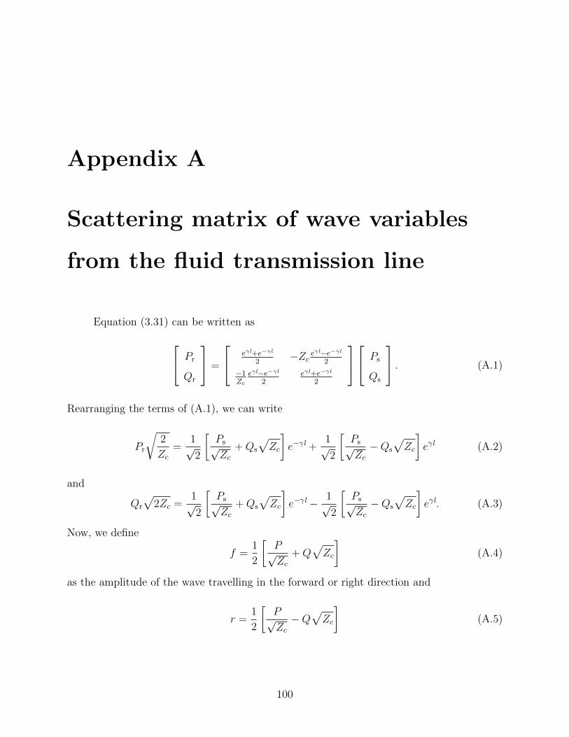
Appendix A

Scattering matrix of wave variables

from the fluid transmission line

Equation (3.31) can be written as

Pr

Qr

=

eγl+e−γl

2−Zc e

γl−e−γl2

−1Zc

eγl−e−γl2

eγl+e−γl

2

Ps

Qs

. (A.1)

Rearranging the terms of (A.1), we can write

Pr

√2

Zc=

1√2

[Ps√Zc

+Qs

√Zc

]e−γl +

1√2

[Ps√Zc−Qs

√Zc

]eγl (A.2)

and

Qr

√2Zc =

1√2

[Ps√Zc

+Qs

√Zc

]e−γl − 1√

2

[Ps√Zc−Qs

√Zc

]eγl. (A.3)

Now, we define

f =1

2

[P√Zc

+Q√Zc

](A.4)

as the amplitude of the wave travelling in the forward or right direction and

r =1

2

[P√Zc−Q

√Zc

](A.5)

100

as the amplitude of the wave travelling in the reverse or left direction.

In a matrix form,

f

r

=1

2

1√Zc

√Zc

1√Zc−√Zc

P

Q

. (A.6)

Let fs and rs denote the right and left going waves at the source with the pressure and flow

rate values as Ps and Qs, fr and rr are their corresponding values at the destination with

the pressure and flow rate values as Pr and Qr. The source and destination are the two ends

of a long pipe. Then, (A.6) can be used to relate the forward and reverse waves at source

and destination with their corresponding pressure and flow rate values as fs

rs

=1

2

1√Zc

√Zc

1√Zc−√Zc

Ps

Qs

. (A.7)

and fr

rr

=1

2

1√Zc

√Zc

1√Zc−√Zc

Pr

Qr

. (A.8)

Using (3.30) in (A.7)

fs

rs

=1

2

1√Zc

√Zc

1√Zc−√Zc

cosh(γl) Zc sinh(γl)

1Zc

sinh(γl) cosh(γl)

Pr

Qr

. (A.9)

Equation (A.8) can be rearranged as

Pr

Qr

=

√Zc √Zc1√Zc

−1√Zc

fr

rr

. (A.10)

Thus, (A.9) becomes

fs

rs

=1

2

1√Zc

√Zc

1√Zc−√Zc

cosh(γl) Zc sinh(γl)

1Zc

sinh(γl) cosh(γl)

√Zc √Zc1√Zc

−1√Zc

fr

rr

(A.11)

101

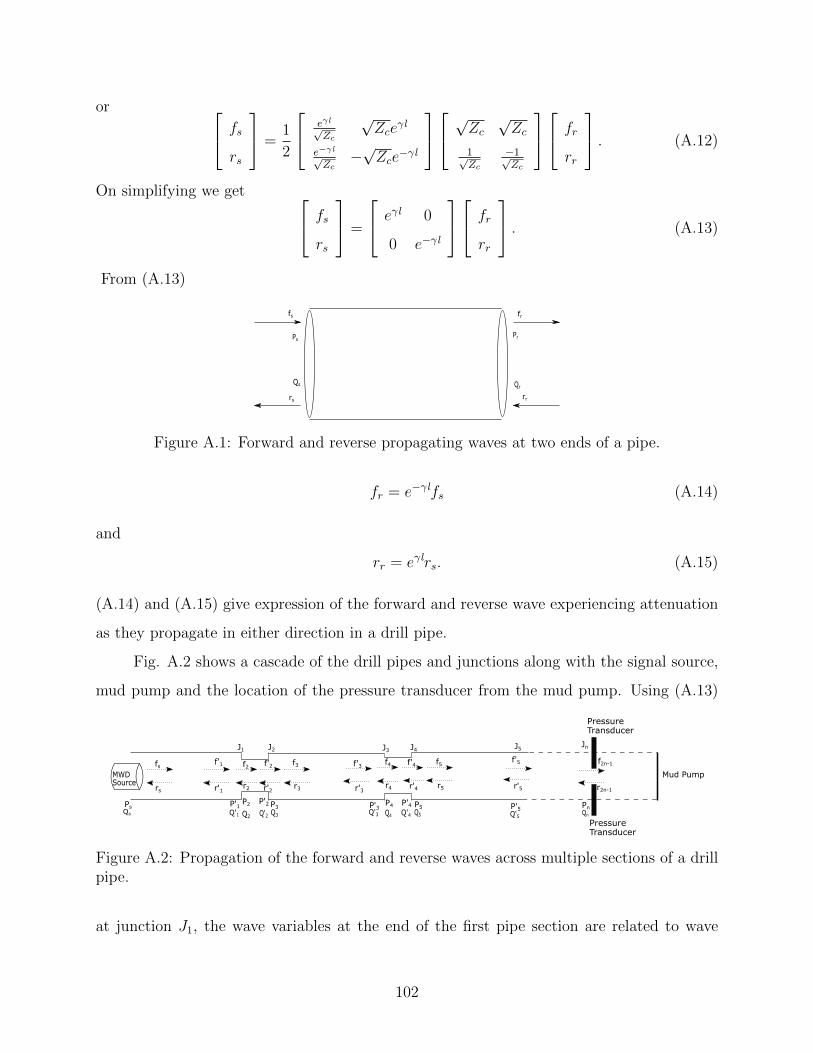
or fs

rs

=1

2

eγl√Zc

√Zce

γl

e−γl√Zc−√Zce

−γl

√Zc √Zc1√Zc

−1√Zc

fr

rr

. (A.12)

On simplifying we get fs

rs

=

eγl 0

0 e−γl

fr

rr

. (A.13)

From (A.13)

Ps Pr

fs

rs

fr

rr

Qs Qr

Figure A.1: Forward and reverse propagating waves at two ends of a pipe.

fr = e−γlfs (A.14)

and

rr = eγlrs. (A.15)

(A.14) and (A.15) give expression of the forward and reverse wave experiencing attenuation

as they propagate in either direction in a drill pipe.

Fig. A.2 shows a cascade of the drill pipes and junctions along with the signal source,

mud pump and the location of the pressure transducer from the mud pump. Using (A.13)

MWD Source

J1 J2 J3 J4J5

P'1PsP2 P3 P'3

P4 P5 P'5

fs

rs

f'1

r'1

f2

r'2

f3

r3

f'3

r'3

f4

r4

f5

r5

f'5

r'5

Jn

r2n-1

Pn

f2n-1

Pressure Transducer

Pressure Transducer

Mud Pump

f'2

r2

f'4

r'4

Qs Q'1 Q2

P'2

Q'2 Q3 Q'3 Q4

P'4Q'4 Q5 Q'5 Qn

Figure A.2: Propagation of the forward and reverse waves across multiple sections of a drillpipe.

at junction J1, the wave variables at the end of the first pipe section are related to wave

102

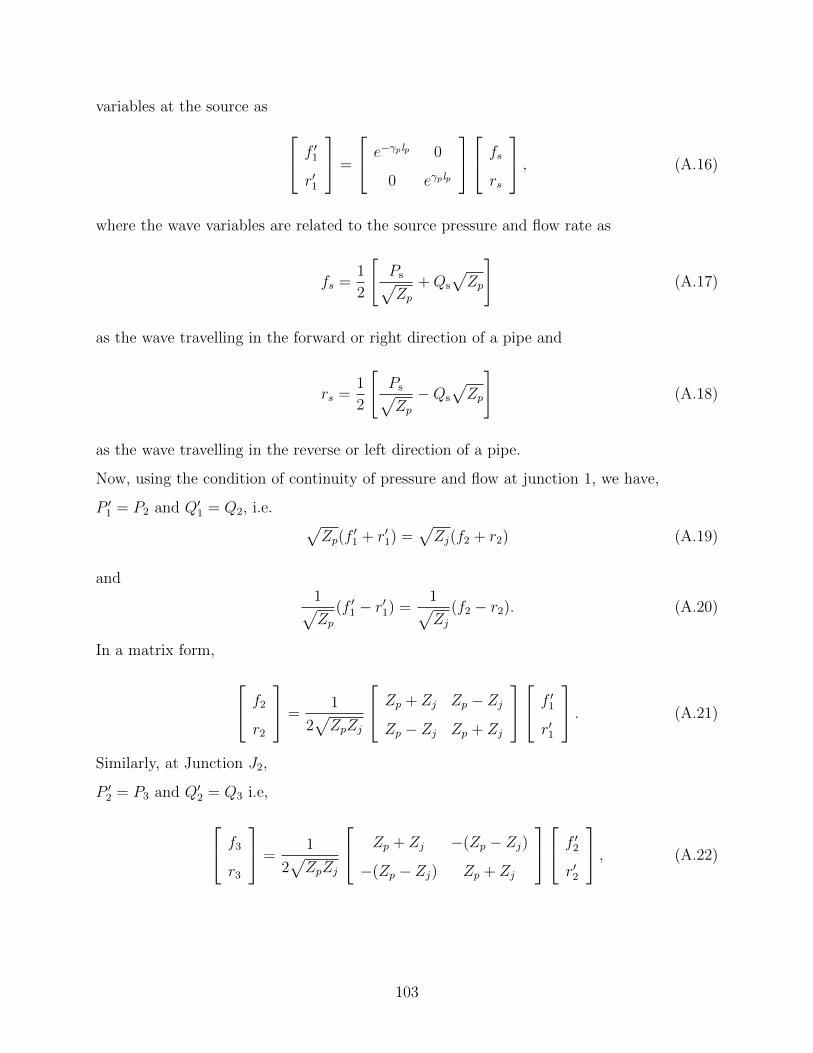
variables at the source as f ′1

r′1

=

e−γplp 0

0 eγplp

fs

rs

, (A.16)

where the wave variables are related to the source pressure and flow rate as

fs =1

2

[Ps√Zp

+Qs

√Zp

](A.17)

as the wave travelling in the forward or right direction of a pipe and

rs =1

2

[Ps√Zp−Qs

√Zp

](A.18)

as the wave travelling in the reverse or left direction of a pipe.

Now, using the condition of continuity of pressure and flow at junction 1, we have,

P ′1 = P2 and Q′1 = Q2, i.e. √Zp(f

′1 + r′1) =

√Zj(f2 + r2) (A.19)

and1√Zp

(f ′1 − r′1) =1√Zj

(f2 − r2). (A.20)

In a matrix form,

f2

r2

=1

2√ZpZj

Zp + Zj Zp − ZjZp − Zj Zp + Zj

f ′1

r′1

. (A.21)

Similarly, at Junction J2,

P ′2 = P3 and Q′2 = Q3 i.e,

f3

r3

=1

2√ZpZj

Zp + Zj −(Zp − Zj)

−(Zp − Zj) Zp + Zj

f ′2

r′2

, (A.22)

103

where f ′2

r′2

=

e−γj lj 0

0 eγj lj

f2

r2

. (A.23)

Thus, the wave variables at the end of the second pipe can be written as f ′3

r′3

=

e−γplp 0

0 eγplp

f3

r3

. (A.24)

Substituting (A.16), (A.21) and (A.22) in (A.24) assuming the length of the junction to be

zero, i.e. lj ≈ 0, and performing matrix chain multiplication, the right and left travelling

waves at the end of the second pipe can be related to the corresponding waves at the source

as f ′3

r′3

=

e−2γplp 0

0 e2γplp

fs

rs

. (A.25)

Equation (A.25) can be generalized to represent the wave flowing in any direction at any

end section of a pipe. If we consider the pressure transducer to be located at the end of

nth section, the forward and reverse travelling waves at nth junction as recorded by pressure

transducer can be related to the the corresponding waves at source as f ′2n−1

r′2n−1

=

e−nγplp 0

0 enγplp

fs

rs

. (A.26)

(A.26) can be re-arranged in the form of T-parameters as

rs

fs

=

e−nγplp 0

0 enγplp

r′2n−1

f ′2n−1

. (A.27)

We can also re-write (A.27) in terms of S-parameters as

rs

f ′2n−1

=

0 e−nγplp

e−nγplp 0

fs

r′2n−1

. (A.28)

(A.27) shows that with the length of junction neglected, the attenuation behaviour of the

104

pressure waves in a cascaded system of the drill pipes is identical to that in a single long

drill pipe of length equal to nlp.

105

Appendix B

Transmission line schematics

Fig. B.1 shows an ADS schematic of the transmission line circuit to calculate the

voltage gain of an equivalent single section of a fluid transmission line. The MWD signal

source is represented by a voltage source with an input frequency of 10 Hz. A single drill

pipe is represented as a physical transmission line with length set to 9.144 m (30 ft) and

characteristic impedance of 3.7616 × 107 ohm. The source impedance is matched with the

transmission line impedance. The values of relative permeability and relative permittivity

of the transmission line are adjusted as per the value of the velocity of the pressure wave

in a drill pipe, which is equal to 1307 ms−1. The physical transmission line is set with an

attenuation of 5.2716× 10−5/m to represent the attenuation of a 10 Hz pressure wave at the

pipe section. Since the mud pump acts as an open circuit, it is simulated by connecting the

transmission line with a load of very high impedance. The pressure sensor is located at a

distance of 15.24m (50 ft) from the mud pump. The expression VoutVin

then gives the voltage

gain across the transmission line, where Vin represents the source voltage and Vout represents

the voltage recorded by the transducer.

Fig. B.2 shows an ADS schematic of the cascaded transmission lines to represent the

simulation of the cascaded drill pipes. For simplicity, only two junction sections are shown

in the figure. All the parameters of the drill pipe are same as described above. Each junction

is assumed to be of length 0.1524m (0.5 ft). The characteristics impedance of the junction is

5.993× 107 ohm and the velocity at the junction is 1446 ms−1 respectively. The attenuation

of the junction is set to 5.7177 × 10−5/m at 10 Hz. The pressure sensor is located at a

106

Figure B.1: ADS schematic to calculate the voltage gain of a single long transmission line.

distance of 15.24m (50 ft) from the mud pump.

Figure B.2: ADS schematic to calculate the voltage gain of a cascaded transmission line.

107