Chain in Mooring System

Chains in Mooring Systems

Evy Bjørnsen

Civil and Environmental Engineering (2 year)

Supervisor: Arne Aalberg, KTCo-supervisor: Per Jahn Haagensen, KT

Department of Structural Engineering

Submission date: June 2014

Norwegian University of Science and Technology

Department of Structural Engineering Faculty of Engineering Science and Technology

NTNU- Norwegian University of Science and Technology

MASTER THESIS 2014

SUBJECT AREA:

Steel structures

DATE:

9 June 2014

NO. OF PAGES:

121 + 7

TITLE:


Kjettinger i fortøyningssystemer

BY:

Evy Bjørnsen

RESPONSIBLE TEACHER: Associate Professor Arne Aalberg

SUPERVISORS: Associate Professor Arne Aalberg and Professor Per Jahn Haagensen

CARRIED OUT AT: Norwegian University of Science and Technology, Department of Structural Engineering

SUMMARY:

Mooring systems of floating structures consist of long lengths of chain, rope or wire, or a combination of these elements. If a mooring line fails, the floating structure can lose station and cause severe damage to structures and environment as well as economic losses and loss of lives. The overall goal of this study is to find out how mooring chains work as structural components in mooring systems. The theory part of the report includes a study of offshore loading conditions, different types of mooring systems, causes of mooring line failure, failure detection of mooring lines and fatigue. However, there is a special focus on mooring chains. The stress distribution in chain links subjected to pure tension is calculated analytical and numerical. Both whole and worn stud links and studless links are analyzed.

The residual stresses resulting from proof testing seem to play an important role. When residual stresses are added to the operational stresses, the resulting maximum tensile stress is 3.65 and 3.30 times the nominal stress for stud links and studless links respectively. The maximum tensile stress is located at the link surface at the crown section. Such tensile stress concentrations at the surface of a material are unfavorable due to fatigue crack propagation.

The worn links have a reduction of cross-sectional diameter of 2.6 % to 13.2 %. Wear will reduce the cross-sectional area and cause some sharp edges, but at the same time increase the contact area. The positive effects of wear seem to surpass the negative effects of wear when the wear is moderate.

ACCESSIBILITY:

Open

Institutt for konstruksjonsteknikk

Fakultet for ingeniørvitenskap og teknologi

NTNU – Norges teknisk-naturvitenskapelige universitet

MASTEROPPGAVE VÅREN 2014

Evy Bjørnsen

Kjettinger i fortøyningssystemer


1. Bakgrunn

Oppgaven tar for seg bruk av kjettinger i fortøyningssystemer. Fortøyningssystemer er kritiske for sikker drift av flytende plattformer, og for skip generelt. Kjettinger kan ha et stort omfang av utførelser og kommer i et stort antall kvaliteter og dimensjoner. Kjettinger som er mest brukt for permanente systemer er tunge og kostbare å håndtere. Høyfast stål benyttes ofte for å gi mindre vekt, og valg av kjetting må tilpasses driftsmiljøet. Det er usikkert hvorvidt utmattingsegenskapene øker i takt med statisk styrke til kjettingen.

2. Gjennomføring

Oppgaven kan gjennomføres med følgende aktiviteter:

Det skal gjøres kort rede for bruk av kjettinger i forankringssystemer, typiske utforminger av kjettinger og kjettingløkker, og hvordan styrke og oppførsel beregnes.

Det skal gjøres en litteraturundersøkelse for å finne relevant litteratur om kjettinger, styrke og egenskaper, og numeriske simuleringer for kjettinger.

Beregningsformler og regler for kjettinger skal presenteres og diskuteres.

Det skal velges ut geometri(er) for kjettingløkker for analytiske og numeriske beregninger.

Elementmetodesimuleringer skal gjøres for å se på spenninger og oppførsel til kjettingløkker.

Det skal gjøres analyser for utmatting.

Kandidatene kan i samråd med faglærer velge å konsentrere seg om enkelte av punktene i oppgaven, eller justere disse.

3. Rapporten

Oppgaven skal skrives som en teknisk rapport i et tekstbehandlingsprogram slik at figurer, tabeller og foto får god rapportkvalitet. Rapporten skal inneholde et sammendrag, evt. en liste over figurer og tabeller, en litteraturliste og opplysninger om andre relevante referanser og kilder.

Oppgaver som skrives på norsk skal også ha et sammendrag på engelsk. Oppgaven skal leveres igjennom «DAIM».

Sammendraget skal ikke ha mer enn 450 ord og være egnet for elektronisk rapportering.

Masteroppgaven skal leveres innen 10. juni 2014.

Trondheim, 14. januar 2014

Arne Aalberg

Førsteamanuensis, Faglærer

I

Preface This thesis concludes the master degree at the Department of Structural Engineering

at NTNU-Norwegian University of Science and Technology. The work on this master

thesis includes 20 weeks of study during the spring term of 2014.

This thesis focus on theory in addition to analytical and numerical calculations. The

numerical calculations are carried out in the computer program Abaqus 6.12.

Because my prior knowledge of fatigue and offshore structures was limited, I wanted

to include basic theory of offshore structures in addition to more detailed theory from

a structural point of view. I think I have learned a lot and challenged myself by

choosing this field of study.

The target group for this report is structural engineers, students studying structural

engineering and others who know standard mechanics, but unknown to the details

concerning chain design. In addition, people with other academic backgrounds may

find this report interesting. Although this report deals with mooring chains for offshore

application, prior knowledge of offshore structures is not necessary.

I want to thank my supervisors at the Department of Structural Engineering at NTNU,

Arne Aalberg and Per Jahn Haagensen. Thank you for guiding me in my work and

thank you for giving me good advices. I appreciate the casual discussions we have

had and all the relevant literature I have received throughout the semester. You have

clearly stated what you wanted with this study and I appreciate that.

I would also like to thank Ph.D. student Knut Andreas Kvåle at the Department of

Structural Engineering at NTNU for helping me with Abaqus 6.12 when it was much

needed.

This master thesis has been very interesting and educational. I am glad I chose this

task provided by the Department of Structural Engineering at NTNU.

Trondheim, 31st of May 2014

II

III

Abstract Mooring systems of floating structures consist of long lengths of chain, rope or wire,

or a combination of these elements. As part of a station-keeping system, the mooring

lines have to keep the movements of the structure to a minimum. The mooring lines

have to withstand the loads acting on the moored structure in addition to loads acting

directly on the mooring components. If a mooring line fails, the floating structure can

lose station and cause severe damage to structures and environment as well as

economic losses and loss of lives. Awareness of corrosion, wear, fatigue and

relevant loading conditions during design will improve the design and extend the

service life of the structural components.

The overall goal of this study is to find out how mooring chains work as structural

components. The theory part of the report includes a study of offshore loading

conditions, different types of mooring systems, causes of mooring line failure, failure

detection of mooring lines and fatigue. However, there is a special focus on mooring

chains. Offshore standards and recommended practices provide common chain link

designs and minimum mechanical properties of links, but in order to study chain links

as structural components, the stresses and strains are of importance. Normal

stresses in chain links are calculated analytical using classic beam theory and curved

beam theory. In addition, three-dimensional elastoplastic finite element models are

applied for a more detailed investigation on the stress distribution in chain links. The

presented analyses are limited to chains subjected to pure tension, although torsion

and bending due to interlink friction may occur. Both stud links and studless links are

analyzed in the computer program Abaqus 6.12.

Mooring components as chain links enter in operation with a residual stress field

created by the required proof test. However, traditional design of mooring chains

does not consider the presence of residual stresses [1-3]. This study shows that

residual stresses play an important role. When residual stresses are added to the

operational stresses, the resulting maximum tensile stress is 3.65 and 3.30 times the

nominal stress for stud links and studless links respectively. The maximum tensile

stress is located at the link surface at the crown section. Such tensile stress

concentrations at the surface of a material are unfavorable due to fatigue crack

propagation.

Both whole links and worn links are modeled with Abaqus 6.12, using solid elements.

The worn links have a reduction of cross-sectional diameter of 2.6 % to 13.2 %. Wear

will reduce the cross-sectional area and cause some sharp edges, but at the same

time increase the contact area. The positive effects of wear seem to surpass the

negative effects of wear when the wear is moderate.

IV

V

Sammendrag Flytende konstruksjoner blir fortøyd med kjetting, tau eller wire. Som komponenter i

et fortøyningssystem skal fortøyningslinene hindre eller minimere bevegelse av den

flytende konstruksjonen. Førtøyningslinene må ha tilstrekkelig kapasitet til å tåle

laster fra den flytende konstruksjonen i tillegg til miljølaster som virker direkte på

linene. Dersom en fortøyningsline går til brudd, kan den flytende konstruksjonen

drifte og forårsake alvorlig skade på konstruksjoner og miljø i tillegg til økonomiske

tap og tap av liv. Dersom korrosjon, slitasje, utmatting og aktuelle lasttilstander blir

tatt i betraktning ved dimensjonering av fortøyningsliner, vil utformingen optimaliseres

og levetiden forlenges.

Det overordnede målet med denne studien er å finne ut hvordan fortøyningskjettinger

oppfører seg som konstruksjonskomponenter i fortøyningssystemer. Teoridelen av

denne rapporten tar for seg offshore-laster, ulike typer fortøyningssystemer, årsaker

til brudd i fortøyningsliner, påvisning av brudd i fortøyningsliner og utmatting.

Offshore standarder og anbefalt praksis setter krav til utforming og minimum

mekaniske egenskaper til kjettingløkker, men for å kunne studere kjettinger som

konstruksjonskomponenter er det spenninger og tøyninger som er av interesse.

Normalspenninger i kjettingløkker er beregnet analytisk ved hjelp av klassisk

bjelketeori og krum bjelketeori. I tillegg er tredimensjonale elastoplastiske modeller

analysert for å få et mer detaljert bilde av spenningsfordelingen i kjettingløkker.

Analysene er begrenset til kjettingløkker med ren strekkbelastning selv om torsjon og

bøying, som følge av friksjon mellom løkker, også kan forekomme. Både stolpeløkker

og stolpeløse løkker er analysert i Abaqus 6.12. Abaqus 6.12 er et data-program som

gjør numeriske beregninger basert på elementmetoden.

Fortøyningskomponenter som kjettingløkker må prøvebelastes før de tas i bruk. Den

påkrevde prøvebelastningen resulterer i restspenninger, men tradisjonell design av

kjetting tar ikke restspenninger i betraktning [1-3]. Dette studiet viser at

restspenninger har stor betydning for det endelige spenningsbildet i en kjettingløkke.

Når restspenninger legges til bruksspenninger, er den resulterende maksspenningen

3,65 og 3,30 ganger større enn nominell spenning for henholdsvis stolpeløkker og

stolpeløse løkker. Maks strekkspenning er på løkkeoverflaten midt mellom innsiden

og utsiden av løkka ved kronepartiet. Store strekkspenninger oppstår også ved

bøyen og i den rette delen i kjettingløkka. Slike spenningskonsentrasjoner er svært

uheldige siden utmattingsriss ofte oppstår i nærheten av disse.

Både hele og slitte løkker er modellert med Abaqus 6.12. De slitte løkkene har en

reduksjon av tverrsnittsdiameteren på 2,6 % til 13,2 %. Slitasje vil redusere

tverrsnittsarealet og forårsake enkelte skarpe kanter, men også forstørre

kontaktarealet mellom to løkker. Det kan virke som om de positive effektene av

slitasje overgår de negative effektene av slitasje når slitasjen er moderat.

VI

Contents

Preface ........................................................................................................................ I

Abstract ..................................................................................................................... III

Sammendrag .............................................................................................................. V

Definitions ................................................................................................................... 1

1. Introduction ............................................................................................................. 7

1.1 General Background ......................................................................................... 7

1.2 Objective of Study ............................................................................................. 8

1.3 Scope of Study .................................................................................................. 8

2. Introduction to Mooring Chains ............................................................................. 10

2.1 Manufacturing and Testing of Material Properties ........................................... 10

2.2 Dimensions ..................................................................................................... 13

2.3 Chain Types -Advantages and Disadvantages ............................................... 14

3. Failure Modes of Materials ................................................................................... 15

3.1 Failure Criteria ................................................................................................ 15

3.2 Ductile Failure ................................................................................................. 16

3.3 Brittle Failure ................................................................................................... 18

3.4 Critical Stress Locations in Chain Links .......................................................... 21

3.5 Stress Concentration Factor ........................................................................... 23

4. Basis for Calculations ........................................................................................... 27

4.1 Capacity of Chains .......................................................................................... 27

4.2 Cross-Sectional Capacity ................................................................................ 28

4.3 Stresses in Curved Beams .............................................................................. 30

4.4 Contact Stress and Contact Area .................................................................... 32

4.4.1 Two Identical Spheres .............................................................................. 33

4.4.2 Two Cylinders With Radius R1 and R2 ...................................................... 33

5. Environmental Loads ............................................................................................ 35

5.1 Loads on Offshore Structures ......................................................................... 35

5.2 Design Criteria ................................................................................................ 36

6. Moorings -Systems and Analysis .......................................................................... 39

6.1 Offshore Structures ......................................................................................... 39

6.2 Mooring Systems ............................................................................................ 40

6.3 Types of Analysis ............................................................................................ 42

7. Failure of Mooring Systems .................................................................................. 47

7.1 Causes of Mooring Line Failure ...................................................................... 47

7.1.1 Out of Plane Bending ............................................................................... 47

7.1.2 Torsion ..................................................................................................... 48

7.1.3 Corrosion .................................................................................................. 49

7.1.4 Wear ......................................................................................................... 52

7.2 Consequences of Mooring Line Failure ........................................................... 52

7.3 Damage Statistics ........................................................................................... 54

8. Fatigue .................................................................................................................. 56

8.1 The Fatigue Process ....................................................................................... 56

8.2 Fatigue Stress and Fatigue Life ...................................................................... 57

8.3 Fatigue Analysis Based on S-N-data .............................................................. 59

8.3.1 Fatigue Damage ....................................................................................... 62

8.3.2 Mean Stress Effects ................................................................................. 63

8.4 Fatigue Analysis Based on Fracture Mechanics ............................................. 65

8.5 Main Factors Influencing the Fatigue Life ....................................................... 68

8.6 Residual Stresses ........................................................................................... 68

8.7 Notches ........................................................................................................... 69

8.8 Corrosion ........................................................................................................ 70

9. Service Life ........................................................................................................... 71

9.1 Inspection ........................................................................................................ 71

9.2 Line Failure Detection ..................................................................................... 72

9.3 Extended Service Life ..................................................................................... 73

10. Static Analysis .................................................................................................... 76

10.1 Analytical Calculations .................................................................................. 76

10.2 Calculations in Focus Konstruksjon 2014 ..................................................... 77

10.3 Comparison of Results .................................................................................. 81

11. Numerical Analysis ............................................................................................. 83

11.1 Input Data ..................................................................................................... 83

11.1.1 Geometry ................................................................................................ 83

11.1.2 Material Properties ................................................................................. 84

11.1.3 Interaction ............................................................................................... 85

11.1.4 Loading and Boundary Conditions .......................................................... 86

11.1.5 Element Type ......................................................................................... 87

11.1.6 Mesh ....................................................................................................... 88

11.2 Results .......................................................................................................... 91

12. Discussion of Results ....................................................................................... 102

12.1 Paths and Stresses ..................................................................................... 102

12.2 Critical Points .............................................................................................. 106

12.3 Deformation of Contact Area ....................................................................... 111

12.4 Fatigue Life Calculations ............................................................................. 111

12.4.1 Fatigue Life Calculations Using S-N-curves and T-N-curves ................ 112

12.4.2 Fatigue Life Calculations Using Numerical Results .............................. 112

12.5 Possible Sources of Error ........................................................................... 113

13. Comparison of Analytical and Numerical Results ............................................. 115

14. Conclusion ........................................................................................................ 116

15. Suggestions for Future Studies ........................................................................ 118

References ............................................................................................................. 119

Appendix A. Unit Load Method ..................................................................................... i

Appendix B. Von Mises Yield Criterion ........................................................................ v

Appendix C. Plastic Capacity ..................................................................................... vii

1

Definitions

General rules

Parameters used in equations are explained in the following section

Formulas are provided with references in the section prior to the equation

Sections based on one reference will include the reference at the beginning of

that section

Abbrevations

ALS Accidental limit state

API American Petroleum Institute

COD Crack opening displacement

CTOD Crack tip opening displacement

DNV Det Norske Veritas

FPS Floating production and storage unit

FPSO Floating production, storage and offloading unit

GPS Global positioning system

HSE Health and Safety Executive

IACS International Association of Classification Societies

ISO International Organization for Standardization

MBL Minimum breaking load

MODU Mobile offshore drilling unit

NS-EN Norwegian standard-European norm

NTNU Norwegian University of Science and Technology

OMAE Offshore Mechanics and Arctic Engineering

OTC Offshore Technology Conference

ROV Remotely operated vehicle

SCF Stress concentration factor

SRB Sulphate reducing bacteria

ULS Ultimate limit state

2

Symbols

Chapter 2

KV Absorbed energy [J]

Chapter 3

σ Normal stress [MPa] E Young's modulus or Modus of elasticity [MPa] ε Strain [-] σp Proportional limit σe Elastic limit fy Yield stress [MPa] εp Plastic strain [-] εe Elastic strain [-] τmax Max shear stress [MPa] σ1 Highest principal stress [MPa] σ3 Lowest principal stress [MPa] σx Normal stress in x-direction [MPa] σy Normal stress in y-direction [MPa] σz Normal stress z-direction [MPa] τxy Shear stress in the xy-plane [MPa] τyz Shear stress in the yz-plane [MPa] τzx Shear stress in the zx-planet [MPa] KI Stress intensity factor for crack mode 1 [MPa√m] KII Stress intensity factor for crack mode 2 [MPa√m] KIII Stress intensity factor for crack mode 3 [MPa√m] β Factor dependent on the structures geometry [-] and loading a Full crack length if the crack evolves from the [mm] edge or half the length if the crack occurs with a distance to the edge of the structure t Thickness [mm] KIC Fracture toughness for crack mode 1 [MPa√m] ac Critical crack length [mm] Ue. Energy needed to extend the crack [J] Ur Strain energy released [J] fu Tensile strength or compressive strength [MPa] Kt Stress concentration factor [-] σmax Maximum stress [MPa] σnom Nominal stress [MPa] Kf Fatigue stress concentration factor [-] SCF Stress concentration factor [-] F Axial load [N] A Cross sectional area [mm2] D Cross-sectional diameter [mm] M Bending moment [Nm] I Moment of inertia [mm4] R Radius of the cross section [mm] r Radius of curvature [mm]

http://no.wikipedia.org/wiki/I




3

B Factor [-]

Chapter 4

Eeff Effective modulus of elasticity [MPa] L Length of chain link [mm] ∆L Elongation of chain link [mm] σx,Ed Design value of normal stress in x-direction [MPa] τEd Design value of shear stress [MPa] fyd Design value of yield stress [MPa] VEd Design value of shear force [N] S Statical moment of area [mm3] NEd Design value of axial force [N] My,Ed Design value of bending moment about the y axis [Nm] Mz,Ed Design value of bending moment about the z axis [Nm] y, z Distance from the centroid of the cross section [mm] to the position where the stress is determined Iy Moment of inertia about the y axis [mm4] Iz Moment of inertia about the z axis [mm4] Wy Elastic section modulus about the y axis [mm3] Wz Elastic section modulus about the z axis [mm3] MRd Design value of elastic moment capacity [Nm] VRd Design value of elastic shear capacity [N] NRd Design value of elastic axial force capacity [N] Mpl,Rd Design value of plastic moment capacity [Nm] Wpl Design value of plastic section modulus [mm3] Npl,Rd Design value of plastic axial force capacity [N] Vpl,Rd Design value of plastic shear capacity [N] Av Shear area [mm2] ΤRd Design value of elastic torque capacity [Nm] Τpl,Rd Design value of plastic torque capacity [Nm] τΤ,max Max shear stress as a result of torque [MPa] TEd Design value of torque [Nm] r0 Distance from the axis of rotation to the [mm] position where the stress is determined Ip Polar moment of inertia [mm4] σb Bending stress [MPa] R1 Distance from the center of curvature to [mm] the neutral axis ŕ Distance from the center of curvature to [mm] the centroid of the cross section r1 Distance from the center of curvature to [mm] the position where the stress is determined τ Shear stress [MPa] N Axial force [N] V Shear force [N] A1 = ∫r dA, area of cross section under r Q1 = ∫r r dA a Radius of the contact area [mm] p0 Contact stress [MPa]

4

r2 Distance from the contact area's center to [mm] the position where the stress is determined b Width of contact area [mm] L1 Length of contact area [mm]

Chapter 5

ω Wave frequency [rad/s] H(ω) Transfer function S(ω) Wave spectrum SR(ω) Response spectrum Hs Significant wave height [m] Tp Wave perid [s] Sc Design capacity of chain [N] Smbs Minimum breaking load of a mooring chain [N] sample TC,mean Quasi-static component of the characteristic [N] tensile load TC,dyn Dynamic component of the characteristic [N] tensile load γmean Partial safety factor on mean tension [-] γdyn Partial safety factor on dynamic tension [-]

Chapter 6

T Mooring line tension [N] s Length of mooring line from floating structure [m] to seabed φ Slope between mooring line and the horizontal [rad] or [deg] plane ρ Density of water [kg/m3] g Gravitational acceleration [m/s2] z Water depth [m] w Submerged weight per unit length of the [kg/m] mooring line Dhydro Longitudinal mean hydrodynamic load per [N/m] unit length Fhydro Transverse mean hydrodynamic load per [N/m] unit length h Total water depth of mooring line [m] TH The horizontal component of the mooring [N] line tension at sea level xH Horizontal distance from the anchor to the [m] floating structure Tmax Maximum mooring line tension [N] l Total length of mooring line [m] Fx Horizontal force resultant in local x-direction [N] Fy Horizontal force resultant in local y-direction [N] Mz Torque about the vertical z-axis [Nm]

5

THi Horizontal mooring line tension at sea level [N] of line i

xi Horizontal distance in local x-direction from [m] the center of the floating structure to line i yi Horizontal distance in local y-direction from [m] the center of the floating structure to line i ψi Angle between mooring line and the local x-axis [rad] or [deg] k Linear stiffness [N/m] x Displacement [m] Fx(t) Time dependent external load in the [N] direction of the displacement x m Mass of the floating structure [kg] Amass Added mass [kg] C Linear damping [Ns/m] CV Viscous damping [Ns/m]

Chapter 7

v Volume of material removed [mm3] K Wear coefficient [-] P Applied load [N] d Sliding distance [mm] H Penetration hardness [N/mm2]

Chapter 8

σmin Minimum stress [MPa] σa Stress amplitude [MPa] Δσ Stress range [MPa] σm Mean stress [MPa] Nt Total number of cycles Ni Number of cycles in the initiation stage Np Number of cycles in the propagation stage m Negative inverse slope of the design S-N-curve, slope of region 2 in a log-log plot of fatigue crack growth rate versus stress intensity factor range ā Intercept of the design S-N-curve with the log(N) axis ∆T Tension range [N] M,K Factors [-] Dacc. Accumulated fatigue damage kt Number of stress blocks ni Number of stress cycles in stress block i Nti Number of cycles to failure at constant

6

stress range η Usage factor Sa Limiting value of alternating stress amplitude [MPa] Sm Limiting value of mean stress [MPa] Su Limiting value of tensile strength [MPa] Sy Limiting value of yield stress [MPa] Se Endurance limit or fatigue limit [MPa] ka Surface condition modification factor [-] kb Size modification factor [-] kc Load modification factor [-] kd Temperature modification factor [-] ke Miscellaneous-effects modification factor [-] S'e Rotary-beam endurance limit [MPa] Sf Unnotched fully reversed fatigue limit or the [MPa] fatigue strength a, b Factors [-] Ne Endurance limit life σ'F Fatigue strength coefficient [MPa] f Factor [MPa] ΔK Stress intensity factor range [MPa√m] Kmax Maximum stress intensity factor [MPa√m] Kmin Minimum stress intensity factor [MPa√m] C Factor [-] ai Initial crack length [mm] q Notch sensitivity [-]

Chapter 10

G shear modulus [MPa] μ Poisson's ratio [-]

Chapter 12

S11 Stress component in x-direction [MPa] S22 Stress component in y-direction [MPa] U2 Displacement component in y-direction [mm]

Master Thesis 2014

7

CHAPTER 1

Introduction

Mooring systems of floating structures consist of long lengths of chain, rope or wire.

Common practice is to combine wire rope of steel, natural fiber or synthetic fiber with

heavy chain. The benefits of such a material combination is that the chain will

increase the stiffness while the rope will reduce the dead load and provide increased

flexibility in areas with large movements. Chains are typically used at the bottom of a

mooring line, connected to the anchor and at the top, connected to the floating

structure. The top and bottom of a mooring line, respectively the splash zone and the

thrash zone, are particularly exposed to corrosion, wear, axial load and bending. The

robust chain is perfect for such harsh conditions.

Mooring lines have to withstand large loads. As part of a station-keeping system, the

mooring lines have to keep the movements of the moored structure to a minimum.

The mooring lines have to withstand loads on the moored structure in addition to

loads acting directly on the mooring components. The environmental loads from

wind, waves and currents may be large during extreme weather. Such large

environmental loads are normally accounted for. The load with a return period of at

least 100 years is considered when designing mooring components. Usually, the

mooring lines are designed for an operational life of 20 years.

Periodic inspections are necessary to monitor the structural integrity of mooring lines.

If a mooring line fails, the floating structure can lose station and cause severe

damage to structures and environment, economic losses and loss of lives.

Failure of offshore components are mostly brittle although the material is ductile.

Brittle failure in a normally ductile material, such as structural steel, is often caused

by fatigue. Fatigue is a long-term degradation process in materials undergoing cyclic

loading. Although the maximum cyclic load is well below the elastic limit of the

material, cracks will initiate and propagate causing a sudden failure after a sufficient

number of fluctuations. Fatigue is of great concern because the fatigue life is hard to

predict and fatigue cracks are difficult to detect.

1.1 General Background

The financial costs associated with mooring line failure may be extremely large.

When a damaged or broken mooring line is to be replaced with a new one, the

production on the moored structure is normally shut down for a short period.

The oil and gas industry will of course reduce the probability of failure as much as

possible. Awareness of corrosion, wear, fatigue and relevant loading conditions

during design will improve the design and extend the service life of offshore structural

components.

Master Thesis 2014

8

The Norwegian multinational oil and gas company Statoil ASA is currently

collaborating with the Department of Structural Engineering at NTNU on a project

concerning mooring chains. The project is currently in the initial phase, but will

include experimental testing on chain links subjected to cyclic tensile loading. Three

chain links will be tested at a time in a test rig at one of NTNU's laboratories. The

links will be exposed to saltwater and free corrosion during testing in order to

reproduce real offshore conditions.

This master thesis is a preliminary study for the experimental project on chain links.

1.2 Objective of Study

This study focus on mooring chains in offshore mooring systems.

The overall goal of this study is to find out how chains work as structural components

in mooring systems. In order to do so, a set of secondary goals has to be met:

- Present typical designs and mechanical properties of chain links - Present and discuss formulas used to determine the capacity of chain links - Carry out analytical and numerical calculations on chain links - Study fatigue of offshore structures

1.3 Scope of Study

There are many designs of chain links, such as common links, enlarged links and

end links, but only common links are considered in this study. Some chain links have

a transverse stud connecting the link at midpoint. These links are called stud links.

Both stud links and studless links are analyzed in this study. A chain may be exposed

to different loading conditions, such as axial tensile load, bending and torsion. In the

analyses on chain links, axial load is the only external load. Chain links have complex

geometry and a relative large cross-sectional diameter. When doing simplified

analytical calculations, chain links are divided into straight and curved parts. The

curved parts are considered as curved beams. Unlike for straight beams, the bending

stresses vary in a hyperbolic fashion over the cross section of a curved beam.

Numerous standards, recommended practices, textbooks and conference papers

form the basis for this study. In addition, two different computer programs are used to

help solving structural problems. Focus Konstruksjon 2014 is a beam-element

program used to provide static results in terms of bending moments, shear forces,

axial forces and displacements in two-dimensional models of chain links. The general

purpose finite element program Abaqus 6.12 is used to provide stress distributions in

three-dimensional elastoplastic models of chain links composed of solid elements.

The target group for this report is structural engineers, students studying structural

engineering and others who know standard mechanics, but unknown to the details

concerning chain design. In addition, people with other academic backgrounds may

Master Thesis 2014

9

find this report interesting. Although this report deals with mooring chains for offshore

application, prior knowledge of offshore structures is not necessary.

Master Thesis 2014

10

CHAPTER 2

Introduction to Mooring Chains

2.1 Manufacturing and Testing of Material Properties

Chains are rolled steel bars with the shape of links. The joint in each link is flash butt-welded. This welding method is used to connect steel profiles with large cross sections without any use of filler metal [4]. The two end surfaces are set apart at a predetermined distance. Current is applied to the metal and the gap between the two surfaces creates resistance and produces an arc that melt the metal. When the steel is evenly heated and melted, the end surfaces are pressed together. Impurities in the base metal are forced out and the weld is planed so that the cross-sectional diameter is within the limit of allowable nominal diameter at the weld. If the time interval while the two surfaces are pressed together is too short, all the impurities may not be pressed out of the base metal creating a defective weld.

After welding, the steel is hardened with following tempering. The steel is heated and quenched and then heated up again to temperatures above 570 °C [5]. The quenching and tempering changes the material properties in terms of increased toughness and reduced hardness. The material properties can be controlled by changing the heating time, the heating temperature or the cooling period.

Offshore mooring chains have to satisfy a number of requirements due to design and strength. During manufacturing, the steel bars have to undergo a non-destructive testing in terms of magnetic particle testing, ultrasonic testing or Eddy current testing to detect irregularities. Additionally, the finished chain is visual inspected to ensure that the surface is free of damage and without sharp edges. Control measurements of the dimensions are also required [5].The measurements take place while the chain is stretched out by a tensile load of approximately 10 % of the proof load. At least 5 % of the links must be measured. The average diameter at the crown cannot have a negative tolerance larger than the allowable negative tolerance of the nominal diameter, while the positive tolerance shall not exceed 5 % of the nominal diameter. The largest diameter at the flash weld area shall not exceed 15 % of the nominal diameter. The length and width of links are measured as well. This tolerance may not exceed ± 2.5 % of the nominal values. Five and five links of the completed chain are measured at a time and the length of five links is equal to five nominal link lengths minus eight times the nominal diameter. The accuracy of the length of five links must be within 2.5 %.

Mechanical testing controls the material properties of the steel in the completed chain. Samples are taken from at least one link where one test piece is tested for tensile and nine Charpy V-notch test pieces are impact tested. Ten test pieces are taken from the link as illustrated in Figure 2.1. The test pieces are taken from the butt weld, the side opposite the butt weld and from the crown. The samples should be located at a distance of one-third of the cross sectional radius below the material surface.

Master Thesis 2014

11

Figure 2.1: Position of test pieces [5, p. 20]

The tensile test piece is exposed to a uniaxial tensile force. The yield stress, tensile stress, elongation at fracture and reduction of cross sectional area at fracture are detected.

Five different steel grades are used in chains. The International Association of Classification Society (IACS) denotes the steel grades with an R followed by a number. Steel grade R3S, R4 and R4S are considered as high-strength steel. NS-EN 1993-1-1 [6] is only applicable for normal steel with yield stress up to 460 MPa. Additional rules for high-strength steel with yield stress up to 700 MPa are provided by NS-EN 1993-1-12 [7]. Offshore Standard DNV-OS-E302 [5] provides minimum mechanical properties for different steel grades. The required minimum mechanical properties are listed in Table 2.1.

Table 2.1: Minimum mechanical properties for tensile tested steel in chain cables [5, p. 23]

Steel grade

Yield stress [MPa]

Tensile strength [MPa]

Elongation [%]

Reduction of area [%]

R3 410 690 17 50

R3S 490 770 15 50

R4 580 860 12 50

R4S 700 960 12 50

R5 760 1000 12 50

The impact test records the amount of absorbed energy of the test piece at fracture. The test involves a single blow from a swinging pendulum with known mass and arm, released from a known height. The pendulum transfers energy to a notch in the test piece until the test piece breaks [8]. The difference in potential energy from the start position to the end position of the pendulum indicates how much energy the test piece has absorbed. The amount of absorbed energy is the toughness with unit Joule. The material must have high enough toughness to avoid brittle fracture at the lowest operating temperature that is expected to occur during the design life of the

Master Thesis 2014

12

structure [6]. Offshore Standard DNV-OS-E302 [5] provides minimum toughness for different steel grades. The requirements are listed in Table 2.2.

Table 2.2: Minimum mechanical properties for impact tested steel in chain cables [5, p. 23]

Steel grade

Temperature [° C]

Base material Weld

Average absorbed energy [J]

Absorbed energy of one single test piece [J]

Average absorbed energy [J]

Absorbed energy of one single test piece [J]

R3 0 60 45 50 38

-20 40 30 30 23

R3S 0 65 49 53 40

-20 45 34 33 25

R4 -20 50 38 36 27

R4S -20 56 42 40 30

R5 -20 58 44 42 32

The letter K is used in conjunction with absorbed energy and represent the amount of energy that is required to break a test piece by impact testing [9]. The letter V or U is used in addition to K and indicates whether the notch in the test piece is V-or U-shaped. The number 2 or 8 is used in subscript and indicates the radius of the tip of the pendulum, such as KV8.

The toughness of steel is strongly dependent on environmental conditions, such as temperature. This is seen by plotting the absorbed energy as a function of test temperature for a given shape of specimen [9]. This energy/temperature curve, or KV/T curve, is created by plotting the test results at different temperatures. The shape of the curve depends on the material, the shape of specimen and the impact velocity. A typical KV/T-curve has an upper-shelf zone, a transition zone and a lower-shelf zone as sketched in Figure 2.2. From the figure, you see that the toughness turns from low to high values within a small temperature range. The probability of brittle failure increases with decreasing temperatures.

1. Upper-shelf zone 2. Transition zone 3. Lower-shelf zone Figure 2.2: Typical S-shaped energy/temperature curve [9, p. 17]

Master Thesis 2014

13

The energy/temperature curve is S-shaped and the toughness increases with increasing temperatures. "The fracture surface of Charpy test is often rated by the percentage of shear fracture which occurs. The greater the percentage of shear fracture, the greater the notch toughness of the material. The fracture surface of most Charpy specimens exhibit a mixture of both shear and cleavage (brittle) fracture. Because the rating is extremely subjective, it is recommended that it not be used in specifications [9, p. 14 (Annex C)]."

2.2 Dimensions

There are primarily two types of chain links, stud links and studless links. Stud links have, as the name implies, a transverse stud that connects the link at midpoint. The design of stud links is standardized and described in ISO 1704 [10]. The design of studless links is not standardized, but it is common practice to use the dimensions provided by IACS W22 [11]. New link designs have to go through rigorous testing before use to ensure that the requirements given in standards and other regulations are met.

Common stud links have length 6.00 D, width 3.60 D and an inner link radius equal to 0.65 D. Common studless links have length 6.00 D, width 3.35 D and an inner link radius equal to 0.60 D. The letter D stands for nominal diameter [10, 11]. Common link design is sketched in Figure 2.3.

Enlarged links can be used as connectors between common links and end links [10]. The nominal diameter of the enlarged links is 10 % larger than the nominal diameter of the common links, giving D1 = 1.10 D. The length and width of enlarged links are calculated by replacing D with D1 in the formulas for common links. The increased diameter of enlarged links result in increased strength. Thus, enlarged links are ideal in critical areas with large loads

a) Side view of chain link b) Stud link [10, p. 4] c) Studless link [10, p. 4] l = 6.00 D, w = 3.60 D l = 6.00 D, w = 3.35 D p = 4.00 D Figure 2.3: Common link design. The l is the total length and the w is the total width of chain links. The D is the nominal cross-sectional diameter

Master Thesis 2014

14

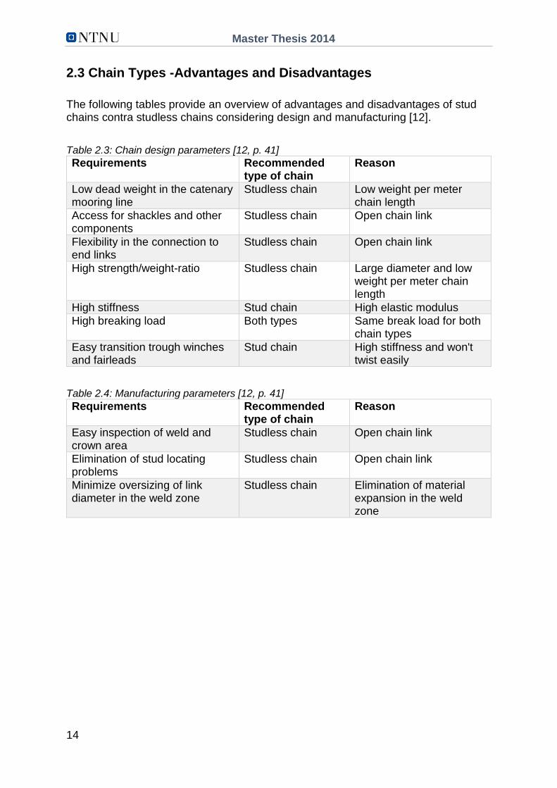
2.3 Chain Types -Advantages and Disadvantages

The following tables provide an overview of advantages and disadvantages of stud chains contra studless chains considering design and manufacturing [12].

Table 2.3: Chain design parameters [12, p. 41]

Requirements Recommended type of chain

Reason

Low dead weight in the catenary mooring line

Studless chain Low weight per meter chain length

Access for shackles and other components

Studless chain Open chain link

Flexibility in the connection to end links


High strength/weight-ratio Studless chain Large diameter and low weight per meter chain length

High stiffness Stud chain High elastic modulus

High breaking load Both types Same break load for both chain types

Easy transition trough winches and fairleads

Stud chain High stiffness and won't twist easily

Table 2.4: Manufacturing parameters [12, p. 41]

Requirements Recommended type of chain

Reason

Easy inspection of weld and crown area


Elimination of stud locating problems


Minimize oversizing of link diameter in the weld zone

Studless chain Elimination of material expansion in the weld zone

Master Thesis 2014

15

CHAPTER 3

Failure Modes of Materials

Materials are often categorized as brittle or ductile. When a brittle material gets plastic deformations, fracture occurs. A ductile material on the other hand, can have large plastic deformations before fracture occurs. Structural steel is ductile under normal conditions, but if the material contains cracks large enough to be seen, it may experience brittle fracture.

This chapter deals with brittle and ductile failure and failure criteria.

3.1 Failure Criteria

A failure criterion estimates whether a state of stress will lead to yielding or fracture in an isotropic material. In order to choose an appropriate failure criterion, one needs to know if the fracture is brittle or ductile. Choice of failure critera depends not only on the type of material, but also on other conditions, such as loading and temperature [13]. For example, low temperatures can change the material from ductile to brittle.

Figure 3.1: Stress-strain curve for brittle and ductile materials. Brittle materials fracture at small strains, while ductile materials fracture only after significant plastic strains. Ductile materials absorb more energy than brittle materials. The amount of absorbed energy corresponds to the shaded area under the curves and depends partly on type of loadling, time of loading and material temperature. This is an idealized example in which both materials have the same yield stress and tensile strength. Taken from Wikipedia [13.10.2010; 26.02.2014]: http://en.wikipedia.org/wiki/File:Brittle_v_ductile_stress-strain_behaviour.png

Failure criteria are just rules designed to fit experimentally observed material behavior, and usually restricted to linear elastic material behavior [13]. No criterion is best under all circumstances. For example, high material temperatures and high hydrostatic pressure will change the behavior of some materials from brittle to

http://www.microsofttranslator.com/bv.aspx?from=&to=en&a=http%3A%2F%2Fen.wikipedia.org%2Fwiki%2FFile%3ABrittle_v_ductile_stress-strain_behaviour.png

http://www.microsofttranslator.com/bv.aspx?from=&to=en&a=http%3A%2F%2Fen.wikipedia.org%2Fwiki%2FFile%3ABrittle_v_ductile_stress-strain_behaviour.png

Master Thesis 2014

16

ductile. Experiments have shown that materials can withstand high hydrostatic pressure without yielding.

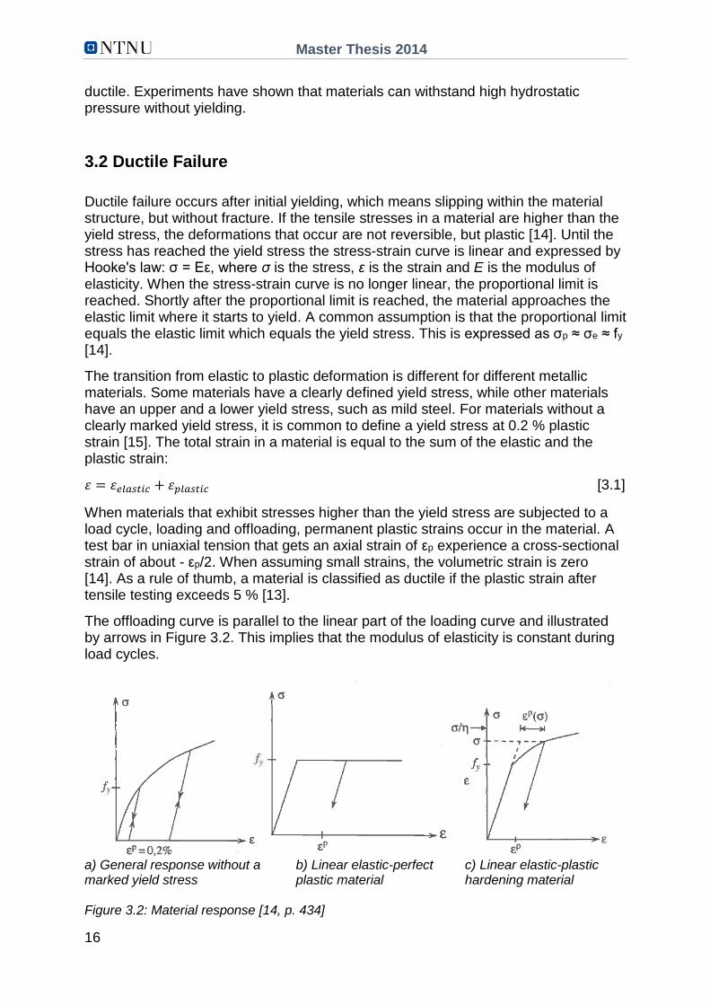
3.2 Ductile Failure

Ductile failure occurs after initial yielding, which means slipping within the material structure, but without fracture. If the tensile stresses in a material are higher than the yield stress, the deformations that occur are not reversible, but plastic [14]. Until the stress has reached the yield stress the stress-strain curve is linear and expressed by Hooke's law: σ = Eε, where σ is the stress, ε is the strain and E is the modulus of elasticity. When the stress-strain curve is no longer linear, the proportional limit is reached. Shortly after the proportional limit is reached, the material approaches the elastic limit where it starts to yield. A common assumption is that the proportional limit equals the elastic limit which equals the yield stress. This is expressed as σp ≈ σe ≈ fy [14].

The transition from elastic to plastic deformation is different for different metallic materials. Some materials have a clearly defined yield stress, while other materials have an upper and a lower yield stress, such as mild steel. For materials without a clearly marked yield stress, it is common to define a yield stress at 0.2 % plastic strain [15]. The total strain in a material is equal to the sum of the elastic and the plastic strain:

𝜀 = 𝜀𝑒𝑙𝑎𝑠𝑡𝑖𝑐 + 𝜀𝑝𝑙𝑎𝑠𝑡𝑖𝑐 [3.1]

When materials that exhibit stresses higher than the yield stress are subjected to a load cycle, loading and offloading, permanent plastic strains occur in the material. A test bar in uniaxial tension that gets an axial strain of εp experience a cross-sectional strain of about - εp/2. When assuming small strains, the volumetric strain is zero [14]. As a rule of thumb, a material is classified as ductile if the plastic strain after tensile testing exceeds 5 % [13].

The offloading curve is parallel to the linear part of the loading curve and illustrated by arrows in Figure 3.2. This implies that the modulus of elasticity is constant during load cycles.

a) General response without a b) Linear elastic-perfect c) Linear elastic-plastic marked yield stress plastic material hardening material Figure 3.2: Material response [14, p. 434]

Master Thesis 2014

17

Hardened material achieves a higher elastic limit and yield stress than a similar material without hardening. The yield stress in a hardened material must be found experimentally [14].

The following two yield criteria are often used in case of ductile material behavior:

Tresca's yield criterion, also called maximum shear stress criterion, assumes that the material starts to yield when the maximum shear stress exceeds a limiting value. Yielding occurs when [13]:

(𝜎1−𝜎3)

𝑓𝑦𝑑≥ 1 [3.2]

τmax –Max shear stress = (σ1-σ3)/2 σ1 > σ2 > σ3 σ1 –Highest principal stress σ2 –Intermediate principal stress σ3 –Lowest principal stress fy –Design value of yield stress

Von Mises' yield criterion assumes that the material starts to yield when the strain energy of distortion per unit volume reaches a limiting value [13]. Yielding occurs when:

(𝜎𝑥−𝜎𝑦)2

+(𝜎𝑦−𝜎𝑧)2

+(𝜎𝑧−𝜎𝑥)2+6(𝜏𝑥𝑦 2 + 𝜏𝑦𝑧

2 + 𝜏𝑧𝑥 2 )

2 𝑓𝑦𝑑 2 ≥ 1 [3.3]

σx –Normal stress in x-direction σy –Normal stress in y-direction σz –Normal stress z-direction τxy –Shear stress in the xy-plane τyz –Shear stress in the yz-plane τzx –Shear stress in the zx-planet fyd –Design value of yield stress

Figure 3.3 shows the failure envelopes obtained by using Tresca's yield criterion and von Mises' yield criterion. If a stress state is located within the respective envelope, there will be no yielding in the material [13]. In a state of pure shear stress, the disagreement between the two criteria is largest when σx = 2 σy or when σy = 2 σx. The maximum difference obtained by using one criterion relative to another is 14.5 %.

Master Thesis 2014

18

Figure 3.3: Failure envelopes for plane stress in terms of principal stresses by using Tresca's yield criterion and von Mises' yield criterion [13, p. 58, edited]

3.3 Brittle Failure

Brittle failure may occur in the presence of cracks in a structure. A typical crack arises from high stresses and evolves with increasing load, load cycles or corrosion [13]. In tension, cracks develop perpendicular to the load direction and in compression, cracks develop with an angle to the load direction. When the cracks reach a critical length, the structure will experience a sudden fracture without warning. Brittle fracture can be minimized by drilling holes in the structure to prevent further crack propagation or by applying deformations that prevent cracks.

The large stress concentration near a crack tip causes the material there to lose ductility [13]. There are three crack modes. They depend on the loading condition as illustratd in Figure 3.4. The high stresses near the crack tip will, due to the Poisson effect, result in compression in the thickness direction. However, the volume with highly stressed material is very small, so the contraction is prevented by adjacent material with much lower stresses. The material near the crack tip is therefore exposed to triaxial tension, which favors fracture rather than plastic flow.

Figure 3.4: The three crack modes: Mode 1, 2, and 3 are caused by, respectively, tensile load, shear load and torsion. Taken from Diagram [undated; 26.02.2014]: http://thediagram.com/12_3/thethreemodes.html

A crack may be categorized as one of three crack modes illustrated in Figure 3.4. Mode 1 is normally used, but a mix of different modes is also possible [13]. For each mode, a stress intensity factor is calculated and compared with an upper value. This upper value is called fracture toughness and represent the resistance to brittle fracture.

http://www.microsofttranslator.com/bv.aspx?from=&to=en&a=http%3A%2F%2Fthediagram.com%2F12_3%2Fthethreemodes.html

Master Thesis 2014

19

The stress intensity factor is termed KI for mode 1, KII for mode 2 and KIII for mode 3 and describes the stress field near the crack tip. The tensile stresses in the area around the crack tip are usually very high, resulting in plastic strains. Anyway, the expression of the stress intensity factor is based on linear elastic material behavior and accurate only when the plastic strains are local and limited to a small area near the crack tip. The stress intensity factor has unit MPa√m, and found by using Equation 3.4 [13]:

𝐾I = 𝛽𝜎 √𝜋 𝑎 [3.4]

β –Dimensionless factor dependent on the structures geometry and loading. Approximately equal to 1.0 σ –Nominal stress that would exist if the crack were absent a –Full crack length if the crack evolves from the edge or half the length if the crack occurs with a distance to the edge of the structure

The shear stress is used instead of, or in addition to, the nominal normal stress in Equation 3.4 for crack mode 2 and 3.

Fracture toughness can be found experimentally by using COD-tests (crack opening displacement test). For thin plates, the fracture toughness is a function of the plate thickness, t, but as the plate thickness increases, the toughness is found regardless of t [13]. This has to do with the size effect and that a material tends to have a certain number of flaws per unit volume. Thus, a thin structural part is less likely to include a flaw of critical size. The fracture toughness is temperature dependent and may change drastically at temperatures close to 0 °C. In rolled steel bars, the fracture toughness also depends on the crack direction with respect to the direction of rolling. The fracture toughness for crack mode 1 is [13]:

𝐾𝐈𝐂 = 𝛽(𝑎𝑐) 𝜎√𝜋 𝑎𝑐 [3.5]

When:

𝑡 ≥ 2.5 (𝐾𝐈𝐂

𝑓𝑦)

2

, 𝑎 ≥ 2.5 (𝐾𝐈𝐂

𝑓𝑦)

2

[3.6]

ac –Critical crack length fy –Yield stress

Fracture occurs when:

𝐾𝐈 ≥ 𝐾𝐈𝐂 and 𝑎 ≥ 𝑎𝑐 [3.7]

If the crack length is less than required by Equation 3.6, the calculated stress in the structure might exceed the yield stress. Then one should expect yielding rather than brittle failure [13].

When the length of the crack exceeds critical crack length, brittle failure occurs. The critical crack length is found by using energy considerations [13]. The energy needed to extend the crack an amount da is independent of crack length a. Thus, the energy expended to produce the crack varies linearly with a and is denoted Ue. As the crack grows, stresses are reduced in a semicircular area around the edge crack, and stored strain energy is released. The released strain energy varies approximately





Master Thesis 2014

20

quadratically with a and is denoted Ur. When a is large enough for the increment of strain energy released to equal the increment of energy needed to extend the crack, sudden fracture occurs. The crack length equals critical crack length when:

𝑑𝑈𝑒

𝑑𝑎=

𝑑𝑈𝑟

𝑑𝑎 [3.8]

Two failure criteria are normally used for brittle material behavior without considering cracks and critical crack lengths:

The first criterion, maximum normal stress criterion, predict that fracture occurs when the highest principal stress in x-/y- or z-direction exceeds the tensile strength or the compressive strength of the material. The other two principal stresses in a three-dimensional state of stress are neglected [13]. Fracture occurs when:

|𝜎1|

|𝑓𝑢|≥ 1 [3.9]

σ1 –Highest principal stress fu –Tensile strength or compressive strength

The second criterion, Mohr's criterion, takes all three states of stresses into account. A specimen is tested for uniaxial tension, uniaxial compression and pure shear to find the limiting stress in each state of stress [13]. Mohr-circles are plotted for each state of stress, creating an envelope as illustrated in Figure 3.5. If the Mohr circle to a random state of stress is located within the envelope, the stress will not cause failure. Fracture occurs when:

𝜏𝑚𝑎𝑥 = 𝜎 tan(𝜑) + 𝑐 [3.10]

τmax –Max shear stress σ –Normal stress ϕ –Slope of the failure envelope (angle of internal friction) c –Intercept of the failure envelope with the τ-axis (cohesion)

Mohr's criterion may be used in case of ductile failure, then as a yield criterion, but is normally used in case of brittle failure.

Figure 3.5: Mohr failure envelope for tests to failure in tension, shear and compression. The sketch to the right shows a simplified Mohr failure envelope for tests to failure in tension and compression [13, p. 53, edited]

Master Thesis 2014

21

3.4 Critical Stress Locations in Chain Links

The geometry of chain links leads to complex interaction between forces. Structural parts are exposed to bending, shear, tension and torsion, and often in more than one plane [16]. The risk of failure increases if the chain includes flaws of critical size or if the chain is exposed to fatigue or corrosion.

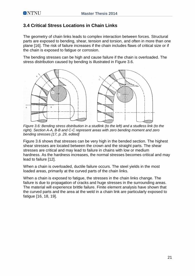
The bending stresses can be high and cause failure if the chain is overloaded. The stress distribution caused by bending is illustrated in Figure 3.6.

Figure 3.6: Bending stress distribution in a studlink (to the left) and a studless link (to the right). Section A-A, B-B and C-C represent areas with zero bending moment and zero bending stresses [17, p. 29, edited]

Figure 3.6 shows that stresses can be very high in the bended section. The highest shear stresses are located between the crown and the straight parts. The shear stresses are critical and may lead to failure in chains with low or medium hardness. As the hardness increases, the normal stresses becomes critical and may lead to failure [12].

When a chain is overloaded, ductile failure occurs. The steel yields in the most loaded areas, primarily at the curved parts of the chain links.

When a chain is exposed to fatigue, the stresses in the chain links change. The failure is due to propagation of cracks and huge stresses in the surrounding areas. The material will experience brittle failure. Finite element analysis have shown that the curved parts and the area at the weld in a chain link are particularly exposed to fatigue [16, 18, 19].

Master Thesis 2014

22

Figure 3.7: Critical locations in studless links exposed to cyclic loading. Fatigue may take

place at point A, B, C, D, E, F or G due to cyclic axial load, bending and/or torsion [16, p. 4]

Critical areas where fatigue may occur is [16]:

Point A: Inner surface of link at weld, stresses in axial direction. This point will be critical primarily because of the weld and the accompanying stress concentration factor. The weld may have residual stresses due to heat treatment or the weld may have a flaw due to impurities or lack of bond between the bar ends. In case of studlinks, the stud may displace, causing high stresses at this point. Point B: Lateral surface of link at weld, stresses in axial direction. This point will receive the highest stress due to out-of-plane bending. Point C: Outer surface of link at weld, stresses in axial direction. This point will receive the highest stress due to in-plane bending. Use of studlinks will reduce the stresses at this point [18]. Point D: Inner surface at crown, stresses in the direction of maximum stress range. This point will receive the highest stress range due to out-of-plane bending. Point E: Inner surface at bend, stresses in the direction of the maximum principal stress. This point will receive the highest stress due to in-plane bending. Point F: Inner surface at bend. Maximum stress range due to torsion is seen at this point. Point G: Crown of link. This point will receive high stresses due to tensile loading.

Master Thesis 2014

23

3.5 Stress Concentration Factor

Stresses in a solid are rarely uniform. Local stress variations may occur in case of

material-inhomogeneity or by abrupt changes in geometry [13]. Material

inhomogeneity includes constituents of foreign materials or small voids in the base

material while geometrical discontinuity include cross-sectional changes, sharp

edges, holes or cracks. The stress concentration will increase in the surrounding area

of the inhomogeneity or the geometrical discontinuity.

The stress concentration factor, Kt, is independent of material properties, but based

on geometry and loading. The stress concentration factor is commonly termed SCF.

For an isotropic and linear elastic material, the stress concentration factor equals

[13]:

𝐾𝑡 =𝜎𝑚𝑎𝑥

𝜎𝑛𝑜𝑚 [3.11]

σmax –Maximum stress in a stress concentration

σnom –Nominal stress

The nominal stress in a chain link does not necessary correspond to actual stresses

in links. The nominal stress is calculated as follows:

σnom = F/2A = 2F/πD2, where F is the external axial tensile load and A is the cross-

sectional area equal to πD2/4, or

σnom = M/2W = 0.5DM/2I = 16M/πD3, where D is the cross-sectional diameter, M is

the external bending moment and I is the moment of inertia to a massive circular

cross section.

The maximum stress in a stress concentration is sometimes difficult to calculate

analytically, but numerical calculations or experimental testing may help finding this

stress. "Elastic stress concentration factors are obtained from the theory of elasticity,

from numerical solutions, or from experimental measurements. The most common

and most flexible numerical method is the finite element method. When using this

method, a model with relatively fine mesh in the areas of steep stress gradients is

required to ensure computational accuracy [20, p. 189-190]."

Charts of stress concentration factors are available in the literature [20]. Figure 3.8

shows a copy of such a chart. The stress concentration factor in Figure 3.8 is due to

opposite U-shaped notches in a circular bar exposed to tension, bending and torsion.

The nominal stress in a notched component is defined as load divided by total gross

area or load divided by net area. Figure 3.8 gives stress concentration factors based

on net area, the cross-sectional area that remains after introduction of notches.

Master Thesis 2014

24

Figure 3.8 a) Stress consentration factor for a U-shaped grooved shaft of circular cross

section in tension. r/D from 0.001 to 0.050 [21, p. 100]

Figure 3.8 b) Stress consentration factor for a U-shaped grooved shaft of circular cross

section in bending. r/D from 0.001 to 0.050 [21, p. 123]

Master Thesis 2014

25

Figure 3.8 c) Stress consentration factor for a U-shaped grooved shaft of circular cross

section in torsion. r/D from 0.001 to 0.050 [21, p.130]

Figure 3.8: Stress concentration factors for a circular bar with opposite U-shaped notches.

The circular bar is exposed to tension, bending and torsion respectively [21]

It is particularly important to keep track of the stress concentrations in a solid when

doing fatigue analyses. A modified stress concentration factor is used for service life

calculations [13]. This fatigue stress concentration factor is denoted Kf and is smaller

than Kt. Stress concentrations may not be of great concern during static loading and

ductile material behavior because yielding redistributes stresses without signs of

fracture.

The stress concentration factor is reduced if sharp edges are smoothed. Common

practice is to drill holes at crack tips to reduce the stress concentration in the

surrounding area and prevent or delay further crack propagation.

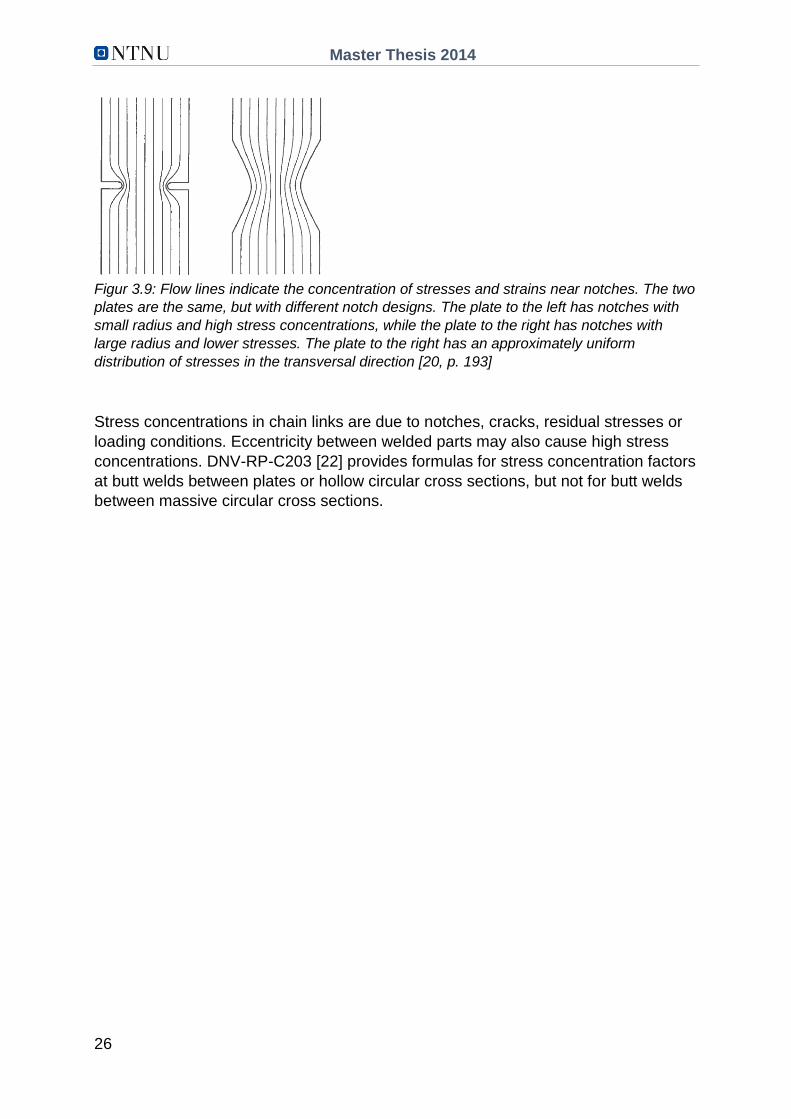
Figure 3.9 sketch flow lines near notches in a plate exposed to axial tension. The flow

lines help to visualize the concentration of stresses and strains [20].

Master Thesis 2014

26

Figur 3.9: Flow lines indicate the concentration of stresses and strains near notches. The two

plates are the same, but with different notch designs. The plate to the left has notches with

small radius and high stress concentrations, while the plate to the right has notches with

large radius and lower stresses. The plate to the right has an approximately uniform

distribution of stresses in the transversal direction [20, p. 193]

Stress concentrations in chain links are due to notches, cracks, residual stresses or

loading conditions. Eccentricity between welded parts may also cause high stress

concentrations. DNV-RP-C203 [22] provides formulas for stress concentration factors

at butt welds between plates or hollow circular cross sections, but not for butt welds

between massive circular cross sections.

Master Thesis 2014

27

CHAPTER 4

Basis for Calculations

Chain links are complex structural parts. The bending stresses cannot be calculated in a traditional manner due to the curved shape of links. Special rules for curved beams as well as general rules in the ultimate limit state are presented in this chapter.

4.1 Capacity of Chains

Formulas used to determine the capacity of chains are purely empirical and based on the strength found experimentally [17].

Offshore standard DNV-OS-E302 [5] provides minimum breaking load and minimum proof load for chains. The minimum breaking load and proof load are based on steel grade and nominal cross-sectional diameter and summarized in Table 4.1. All chains are proof tested to ensure that they can withstand the proof load without any sign of fracture. The proof load is typically 70-80 % of minimum breaking load.

Table 4.1: Minimum breaking load (MBL) and proof load [5, p. 22]. The factor Z in the table is set to D2 (44.0 - 0.08D)

Steel grade R3 R3S R4 R4S R5

Breaking load [kN]

0.0223 Z

0.0249 Z

0.0274 Z

0.0304 Z

0.0320 Z

Proof load [kN]

Stud chain 0.0156 Z1)

0.0180 Z

0.0216 Z

0.0240 Z

0.0251 Z

Studless chain

0.0156 Z1)

0.0174 Z

0.0192 Z

0.0213 Z

0.0223 Z

Weight [kg/m]

Stud chain 0.0219 D2

Studless chain

0.0200 D2 2)

1) Equal to 0.0148 Z according to IACS W22 [11]. 2) Applicable to studless chains with dimensions in accordance with IACS

W22 [11]. For other designs of chains, weight calculations have to be done.

The required minimum breaking load is the same for stud chains and studless chains. The required minimum proof load is slightly smaller for studless chains than for stud chains with steel grade R3S, R4, and R5 R4S. Note that the required proof load for steel grade R3 provided by DNV-OS-E302 [5] differs from the proof load provided by IACS W22 [11].

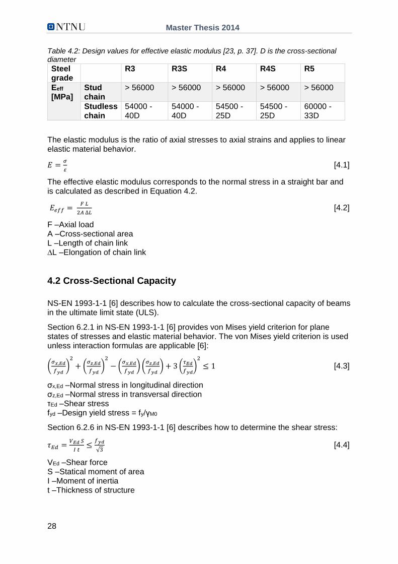
The manufacturer shall provide the effective elastic modulus of the chain. If the effective elastic modulus is unknown, preliminary design values shall be taken as listed in Table 4.2.

Master Thesis 2014

28

Table 4.2: Design values for effective elastic modulus [23, p. 37]. D is the cross-sectional diameter

Steel grade

R3 R3S R4 R4S R5

Eeff [MPa]

Stud chain

> 56000 > 56000 > 56000 > 56000 > 56000

Studless chain

54000 - 40D

54000 - 40D

54500 - 25D

54500 - 25D

60000 - 33D

The elastic modulus is the ratio of axial stresses to axial strains and applies to linear elastic material behavior.

𝐸 =𝜎

𝜀 [4.1]

The effective elastic modulus corresponds to the normal stress in a straight bar and is calculated as described in Equation 4.2.

𝐸𝑒𝑓𝑓 = 𝐹 𝐿

2𝐴 ∆𝐿 [4.2]

F –Axial load A –Cross-sectional area L –Length of chain link ∆L –Elongation of chain link

4.2 Cross-Sectional Capacity

NS-EN 1993-1-1 [6] describes how to calculate the cross-sectional capacity of beams in the ultimate limit state (ULS).

Section 6.2.1 in NS-EN 1993-1-1 [6] provides von Mises yield criterion for plane states of stresses and elastic material behavior. The von Mises yield criterion is used unless interaction formulas are applicable [6]:

(𝜎𝑥,𝐸𝑑

𝑓𝑦𝑑)

2

+ (𝜎𝑧,𝐸𝑑

𝑓𝑦𝑑)

2

− (𝜎𝑥,𝐸𝑑

𝑓𝑦𝑑) (

𝜎𝑧,𝐸𝑑

𝑓𝑦𝑑) + 3 (

𝜏𝐸𝑑

𝑓𝑦𝑑)

2

≤ 1 [4.3]

σx,Ed –Normal stress in longitudinal direction σz,Ed –Normal stress in transversal direction τEd –Shear stress fyd –Design yield stress = fy/γM0

Section 6.2.6 in NS-EN 1993-1-1 [6] describes how to determine the shear stress:

𝜏𝐸𝑑 =𝑉𝐸𝑑 𝑆

𝐼 𝑡≤

𝑓𝑦𝑑

√3 [4.4]

VEd –Shear force S –Statical moment of area I –Moment of inertia t –Thickness of structure

Master Thesis 2014

29

If the y- and z-axes are principal axes in a cross section, the normal stress is as shown in Equation 4.5. According to classic beam theory, the stress σz is negligible compared to σx [24]:

𝜎𝑥,𝐸𝑑 =𝑁𝐸𝑑

𝐴+

𝑀𝑦,𝐸𝑑 𝑧

𝐼𝑦−

𝑀𝑧,𝐸𝑑 𝑦

𝐼𝑧 [4.5]

NEd –Axial force A –Area of cross section My,Ed –Bending moment about the y axis Mz,Ed –Bending moment about the z axis y, z –The distance from the centroid of the cross section to the position where the stress is determined Iy –Moment of inertia about the y axis Iz –Moment of inertia about the z axis Wy –Elastic section modulus about the y axis = Iy/z Wz –Elastic section modulus about the z axis = Iz/y

The von Mises yield criterion is the most common failure criterion for metallic structures. The yield criterion presented in Equation 4.3 apply to two-dimensional states of stress and should only be used in cases where the formulas for interaction between bending, shear and axial force cannot be used [6]. Von Mises yield criterion does not take plastic redistribution of stresses into account and is therefore on the safe side.

Elastic cross-sectional capacities are calculated as follows:

𝑀𝑅𝑑 = 𝑓𝑦𝑑 𝑊 [4.6]

𝑉𝑅𝑑 = 𝑓𝑦𝑑 𝐼 𝑡/√3 𝑆 [4.7]

𝑁𝑅𝑑 = 𝑁𝑝𝑙,𝑅𝑑 = 𝐴 𝑓𝑦𝑑 [4.8]

When bending moment and axial load act simultaneously, the plastic moment capacity is reduced to MN,Rd. The interaction formula is found in section 6.2.9.1 in NS-EN 1993-1-1 [6].

𝑀𝐸𝑑 ≤ 𝑀𝑁,𝑅𝑑 = 𝑀𝑝𝑙,𝑅𝑑[1 − (𝑁𝐸𝑑/𝑁𝑝𝑙,𝑅𝑑)2] [4.9]

Mpl,Rd –Plastic moment capacity = Wpl fyd NEd –Axial force Npl,Rd –Plastic axial force capacity = A fyd

When bending moment, axial load and shear force act simultaneously and the shear force exceeds 50 % of the plastic shear capacity, the plastic moment capacity is further reduced. In this case, a reduced yield stress is used in the expression of moment capacity. The reduced yield stress, as a result of a significantly large shear force, is as described in section 6.2.10 in NS-EN 1993-1-1 [6] and equals:

Master Thesis 2014

30

𝑓𝑦 [1 − ((2𝑉𝐸𝑑/𝑉𝑝𝑙,𝑅𝑑) − 1)2] [4.10]

VEd –Shear force Vpl,Rd –Plastic shear capacity = Av fyd/√3, when there are no stresses resulting from torsion. Av is the shear area and equal to 32 A/37 for circular massive cross sections

The torque must be less than the torque capacity in straight structural parts.

The elastic torque capacity for circular cross sections is [24]:

𝑇𝑅𝑑 = 𝑓𝑦𝑑 𝜋 𝑟3/(2 √3) [4.11]

The plastic torque capacity for circular cross sections is:

𝑇𝑝𝑙,𝑅𝑑 =4

3𝑇𝑅𝑑 [4.12]

A circular cross section subjected to torque does not warp. Thus, only shear deformations and shear stresses are present in the cross section. The shear stresses vary linearly over the cross section and increase with increasing distance from the center of the cross section in an elastic material. Due to St. Venant torsion theory, max shear stress as a result of torque is [24]:

𝜏𝑇,𝑚𝑎𝑥 = 𝑇𝐸𝑑 𝑟0/𝐼𝑝 [4.13]

TEd –Torque r0 –The distance from the axis of rotation to the position where the stress is determined Ip –Polar moment of inertia = 0.5 π r4

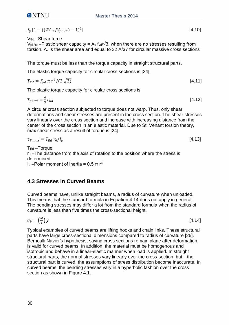
4.3 Stresses in Curved Beams

Curved beams have, unlike straight beams, a radius of curvature when unloaded. This means that the standard formula in Equation 4.14 does not apply in general. The bending stresses may differ a lot from the standard formula when the radius of curvature is less than five times the cross-sectional height.

𝜎𝑏 = (𝑀

𝐼) 𝑦 [4.14]

Typical examples of curved beams are lifting hooks and chain links. These structural parts have large cross-sectional dimensions compared to radius of curvature [25]. Bernoulli Navier's hypothesis, saying cross sections remain plane after deformation, is valid for curved beams. In addition, the material must be homogenous and isotropic and behave in a linear-elastic manner when load is applied. In straight structural parts, the normal stresses vary linearly over the cross-section, but if the structural part is curved, the assumptions of stress distribution become inaccurate. In curved beams, the bending stresses vary in a hyperbolic fashion over the cross section as shown in Figure 4.1.

Master Thesis 2014

31

Figure 4.1: Bending stress variation in a curved beam [25, p. 337]

Because of the hyperbolic bending stress variation, the neutral axis is displaced in the direction of the center of curvature. The neutral axis does no longer coincide with the center of gravity and must be calculated as shown in Equation 4.15 [25].

The distance from the center of curvature to the neutral axis for a circular cross section, is:

𝑅1 = 𝐷2/8(ŕ − √ŕ2 −𝐷2

4) [4.15]

D –Cross-sectional diameter ŕ –The distance from the center of curvature to the centroid of the cross section

The bending stress in the direction of the circumference of the beam, the so-called circumferential stress, is [25]:

𝜎𝑏 =𝑀(𝑅−𝑟1)

𝐴 𝑟1(ŕ−𝑅) [4.16]

The normal stress caused by bending and axial load, is equal to [13]:

𝜎 =𝑁

𝐴+

𝑀(𝑅−𝑟1)

𝐴 𝑟1(ŕ−𝑅) [4.17]

N –Axial force M –Bending moment r1 –The distance from the center of curvature to the position where the stress is determined A –Cross-sectional area

In addition to circumferential stresses, there are radial stresses acting in the radial direction as illustrated in Figure 4.2. Anyway, in a massive cross section the radial stresses are very small and can be neglected.

Master Thesis 2014

32

Figure 4.2: Stresses in a curved beam segment. Radial stress is denoted σr and circumferential stress is denoted σ [25, p. 337]

The shear stresses vary over the cross section, and are at a maximum at the centroid of the cross section. The shear stresses vary with distance r1 from the center of curvature to the position at which the stress is determined [13].

𝜏 =𝑉 𝑅

𝐴(ŕ−𝑅)𝑡 𝑟12 [ŕ𝐴1 − 𝑄1] [4.18]

V –Shear force A1 –Area of cross section under r1, = ∫r1 dA Q1 = ∫r1 r1 dA

The shear stresses are usually small. By using the formulas for shear stresses in straight beams, as described in Chapter 4.2, sufficient accuracy is achieved.

4.4 Contact Stress and Contact Area

Loads are transferred in the contact area between two and two links in a chain. The stresses that arise in the contact area can be described with the help of Hertz analysis:

When two bodies are pressed together, the theoretical contact area is a single point where the stresses are infinitely high and yielding occur instantaneously. In practice, it is not so. The spheres will deform and the contact area will increase. The size of the contact area depends on load intensity, structural geometry and material properties such as elastic modulus and Poisson's ratio [13].

In case of two spheres in contact, the contact area is circular with radius a. The highest stress occur in the middle of the contact area and equals p0 [13]. For two parallel cylinders with length L1, the contact area is rectangular with length L1 and width b with the highest stress in the center of the width, equal to p0. Assumptions like there is no friction in the contact area, the contact area is small compared to the bodies and the Poisson's ratio is equal to 0.3 provides the expressions summarized below. Equation 4.19 to 4.23 give the size of the contact area and Hertz stresses in the contact area for elastic, homogeneous and isotropic bodies in contact [13].

Master Thesis 2014

33

4.4.1 Two Identical Spheres

𝑎 = 0,880(𝐹𝑅

𝐸)1/3 [4.19]

𝑝0 = 0,616 (𝐹 𝐸2

𝑅2 )1/3 [4.20]

𝜎𝑧 = −𝑝0√𝑎2−𝑟2

2

𝑎 [4.21]

F –Axial load R –Radius of cross section E –Elastic modulus a –Radius of the contact area r2 –The distance from the contact area's center to the position where the stress is determined

Figure 4.3: Detail of contact between two identical elastic spheres. The figure shows a Cartesian coordinate system consisting of an r-axis and a z-axis in which the origin is located at the center of the contact area [13, s. 44]

Max shear stress is equal to 0.31p0 and act at a distance of approximately a/2 below the surface of the sphere. During cyclic loading, the shear stresses may result in formation of cracks. These cracks may be difficult to detect because they occur below the surface of the sphere [13].

4.4.2 Two Cylinders With Radius R1 and R2

𝑏 = 3,04√𝐹

𝐿1𝐸(

𝑅1𝑅2

𝑅1+𝑅2) [4.22]

𝑝0 = 0,418√𝐹𝐸

𝐿1(

𝑅1+𝑅2

𝑅1𝑅2) [4.23]

b –Width of contact area L1 –Length of contact area, L ≥ 5b

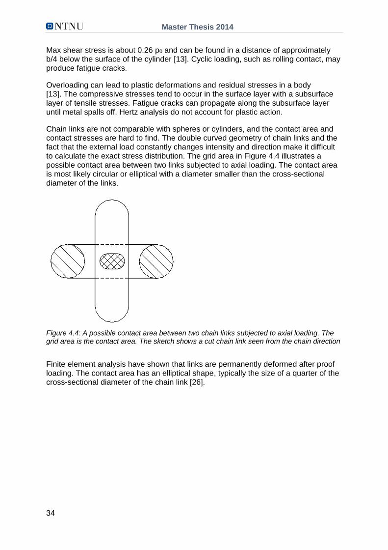
Master Thesis 2014

34

Max shear stress is about 0.26 p0 and can be found in a distance of approximately b/4 below the surface of the cylinder [13]. Cyclic loading, such as rolling contact, may produce fatigue cracks.

Overloading can lead to plastic deformations and residual stresses in a body [13]. The compressive stresses tend to occur in the surface layer with a subsurface layer of tensile stresses. Fatigue cracks can propagate along the subsurface layer until metal spalls off. Hertz analysis do not account for plastic action.

Chain links are not comparable with spheres or cylinders, and the contact area and contact stresses are hard to find. The double curved geometry of chain links and the fact that the external load constantly changes intensity and direction make it difficult to calculate the exact stress distribution. The grid area in Figure 4.4 illustrates a possible contact area between two links subjected to axial loading. The contact area is most likely circular or elliptical with a diameter smaller than the cross-sectional diameter of the links.

Figure 4.4: A possible contact area between two chain links subjected to axial loading. The grid area is the contact area. The sketch shows a cut chain link seen from the chain direction

Finite element analysis have shown that links are permanently deformed after proof loading. The contact area has an elliptical shape, typically the size of a quarter of the cross-sectional diameter of the chain link [26].

Master Thesis 2014

35

CHAPTER 5

Environmental Loads

5.1 Loads on Offshore Structures

Offshore structures are exposed to harsh environments. The many loads lead to complicated load conditions with lots of possible load combinations. In addition, they change in both time and space. The intensity and orientation of the loads vary with time.

The following environmental loads must be considered when designing offshore structures [23]:

- Waves - Wind - Current - Marine growth - Tide and storm surge - Earthquake - Temperature - Snow and ice

Mooring analyses can be performed by applying a frequency domain or a time domain method [23]. The frequency domain is well suited for systems subjected to stationary random loads. The response spectrum can be computed directly from the transfer function and the wave spectrum as shown in Equation 5.1:

𝑆𝑅(𝜔) = |𝐻(𝜔)|2 𝑆(𝜔) [5.1]

ω –Wave frequency = 2π/T H(ω) –Transfer function (e.g. platform heave motion) S(ω) –Wave spectrum SR(ω) –Response spectrum (resulting platform motion due to environmental loads)

The frequency domain method requires that the dynamic response due to low-frequency motions and wave frequency motions result in a system with one degree of freedom and linear equations of motion. This method is usually applied in fatigue analysis of moderate environmental loads where a linearized analysis provides satisfactory results.

The time domain method deals with non-linear equations of motion from drag forces, motion amplitude effects and wave amplitude effects.

The load intensities with a specified return period and the main directions of the loads are used in calculations.

Calculations in the ultimate limit state and the accidental limit state must take the most unfavorable combination of wind, waves and currents into account [23]. The return period of the loads has to be at least 100 years. If the response by currents is relatively small, the load with a return period of 10 years can be used. Fatigue

Master Thesis 2014

36

analysis on permanent moorings shall use a load combination that provides a sufficient accurate service life estimation.

Different parameters are used to describe the environmental conditions. Waves are described by a significant wave height and a peak wave period over a time interval of three hours [23]. Wind is described by a static wind load and a dynamic wind spectrum that addresses the load variation at the location. The static wind load is the average wind speed over a time interval of one hour, 10 meters above the ground. Currents from tides, oceanic circulation patterns and wind are described by a current profile. The current profile provides the static current load, the average current speed at a specified depth.

Table 5.1: Typical environmental loads from waves, wind and currents [23, p. 20-26]

Environmental load Return period

The Norwegian Sea (Haltenbanken)

The North Sea (Troll)

The North Sea (Ekofisk)

Wave Significant wave height, Hs [m]

100 years 16.5 15.0 14.0

Wave period, Tp [s]

100 years 17.0 - 19.0 15.5 - 17.5

15.0 - 17.0

Wind Wind speed [m/s] 100 years 37.0 40.5 34.0

Current Surface current speed [m/s]

10 years 0.9 1.5 0.6

The main orientations of the environmental loads shall form the basis for analyses. In addition, a combination of loads acting in the same direction and directly on one single mooring line has to be analyzed [23].

5.2 Design Criteria

The design criteria applies to structures on land as well as to offshore structures.

The design criteria says that the design capacity must exceed the design loading [23]. Design values are obtained by using partial safety factors as shown in the expression below.

𝐶ℎ𝑎𝑟𝑎𝑐𝑡𝑒𝑟𝑖𝑠𝑡𝑖𝑐 𝑐𝑎𝑝𝑎𝑠𝑖𝑡𝑦

𝑃𝑎𝑟𝑡𝑖𝑎𝑙 𝑠𝑎𝑓𝑒𝑡𝑦 𝑓𝑎𝑐𝑡𝑜𝑟 𝑜𝑛 𝑐𝑎𝑝𝑎𝑐𝑖𝑡𝑦≥ 𝐶ℎ𝑎𝑟𝑎𝑐𝑡𝑒𝑟𝑖𝑠𝑡𝑖𝑐 𝑙𝑜𝑎𝑑 ∙ 𝑃𝑎𝑟𝑡𝑖𝑎𝑙 𝑠𝑎𝑓𝑒𝑡𝑦 𝑓𝑎𝑐𝑡𝑜𝑟 𝑜𝑛 𝑙𝑜𝑎𝑑

A chain is a series system consisting of many components (links). The probability that one of the links have a weakness, and less breaking load than the minimum breaking load, increase with increasing chain length. If one link fails, the entire chain will fail. In short, a long chain is more likely to break than a short chain. This leads to a reduction of capacity of long chains. The minimum breaking load is adjusted to a design capacity for long chains [23]:

Master Thesis 2014

37

𝑆𝑐 = 0,95 𝑆𝑚𝑏𝑠 [5.2]

Sc –Design capacity of chain Smbs –Minimum breaking load of a sample consisting of at least three chain links (the sample can consist of one link if the nominal cross-sectional diameter is 100 mm or more [5])

The characteristic tensile load in a mooring line is divided into a quasi-static and a dynamic component [23]. The quasi-static component, TC,mean, is the characteristic mean tensile load, due to pretension and mean environmental loads. The mean environmental loads are caused by static wind, static current and a mean wave drift force. The dynamic component, TC,dyn, is the characteristic dynamic line tension induced by low-frequency and wave-frequency motions.

Rewriting the design criteria will give the following expression [23]:

𝑆𝐶 ≥ 𝑇𝐶,𝑚𝑒𝑎𝑛 𝛾𝑚𝑒𝑎𝑛 + 𝑇𝐶,𝑑𝑦𝑛 𝛾𝑑𝑦𝑛 [5.3]

The partial safety factors depend on limit state, consequence class and type of analysis [23]. Failure of a mooring system may lead to unacceptable consequences such as loss of lives, collision with other structural parts or significant pollution. Consequence class 1 is used where such consequences are unlikely. Consequence class 2 is used where mooring system failure may lead to consequences of these types.

Quasi-static analysis provides the mooring line response due to average environmental loads and low-frequency motions of the floating structure. Dynamic analysis provides the mooring line response due to wave frequency motions of the floating structure. Analysis must deal with the horizontal displacement, the dead weight, the buoyancy and the elasticity of mooring lines. Dynamic analysis must consider drag forces and inertia forces as well.

Table 5.2: Partial safety factors for ultimate limit state, ULS [23, p. 45]

Consequence class

Type of analysis of wave frequency tension

Partial safety factor on mean tension, γmean

Partial safety factor on dynamic tension, γdyn

1 Dynamic 1.10 1.50

2 Dynamic 1.40 2.10

1 Quasi-static 1.70

2 Quasi-static 2.50

Table 5.3: Partial safety factors for accidental limit state, ALS [23, p. 46]

Consequence class

Type of analysis of wave frequency tension

Partial safety factor on mean tension, γmean

Partial safety factor on dynamic tension, γdyn

1 Dynamic 1.00 1.10

2 Dynamic 1.00 1.25

1 Quasi-static 1.10

2 Quasi-static 1.35

Master Thesis 2014

38

If all the mooring lines in a mooring system are the same, the analysis is limited to the most loaded line. If the mooring lines are different, all lines must be analyzed [23]. The largest tensile load is close to the sea level where the slope of the line is at its steepest. If the mooring line is made up of various components, such as chain, wire and rope, the analysis must include the most loaded area of each component.

Master Thesis 2014

39

CHAPTER 6

Moorings -Systems and Analysis

6.1 Offshore Structures

Offshore structures are used in oil and gas industry all over the world. There are mainly two types of offshore structures: floating structures and fixed structures standing on the seabed [27]. Fixed structures are costly, not to mention challenging in deep waters. Floating structures are easier to dock and well suited in deep water. Figure 6.1 illustrates five different types of offshore structures.

Figure 6.1: Five types of offshore structures. From left to right there are: two types of fixed structures, a semi-submersible platform, a floating production unit and a tension leg platform [28, p. 2]

Mooring lines are used to keep floating structures at a fixed location. Lines must withstand forces from the moving floating structure and from the environmental loads that act directly on the mooring lines. Some mooring lines are prestressed with the help of winches in order to minimize the movements of the moored structure.

Floating structures, with the exception of tension leg platforms, have six degrees of freedom as shown in Figure 6.2 [27]. Tension leg platforms have such a strong buoyancy that the vertical mooring lines, called tendons or tethers, are always in tension. This makes the platform fixed in the vertical direction and three of the degrees of freedom are neglected. The resulting degrees of freedom are surge, sway and yaw, denoted 2, 3 and 4 in Figure 6.2.

Master Thesis 2014

40

Figure 6.2: A rigid body has six degrees of freedom in a three-dimensional space: three displacements and three rotations. 1, 2, 3, 4, 5 and 6 are respectively heave, surge, sway, yaw, roll and pitch. Taken from Wikimedia [12.11.2013; 12.03.2014]: http://commons.wikimedia.org/wiki/File:Brosen_shipsmovemensonthewave.svg

Floating production and storage units, also called FPSO or FPS, are used to refine and store oil and gas [27]. Such units are especially beneficial in areas where piping is costly. Floating production units are far more economical than large oil platforms in small oil fields with short service lives. Several types of mooring systems are used to moor floating production units. Spread mooring is used in shallow waters or in areas sheltered from environmental loads. Using spread mooring, the FPSO is moored with lines spread out from the front and back of the ship-shaped structure. In deep water and harsh environments, turrets are widely used. Then the FPSO is connected to the mooring system in one single point and free to rotate about the vertical axis. When the FPSO rotates due to the direction of the largest environmental load, the total loading on the unit is reduced.

Semi-submersible platforms are widely used as drilling rigs, production platforms or platforms for heavy lift cranes [27]. These platforms are multi-legged floating structures with large slabs. The legs are interconnected below sea level to pontoons, which are horizontal buoyant parts. The pontoons are attached to mooring lines that extend down to anchors at the seabed. A special type of semi-submersible platform is the spar platform. A spar platform is a platform on a huge vertical cylindrical tube that extends well below sea level. The tube is divided into sections where the upper part is a buoyancy chamber and the lower part contains permanent ballast to stabilize the structure. The vertical pipe is attached to mooring lines that extend down to piles or foundations on the seabed.

6.2 Mooring Systems

Mooring and station-keeping of offshore structures is necessary in order to control movements of floating structures and keep the crew on offshore structures safe during weather extremes. The most common station-keeping systems are [27]:

- Catenary mooring - Taut mooring - Dynamic positioning system - Tension leg mooring

http://www.microsofttranslator.com/bv.aspx?from=&to=en&a=http%3A%2F%2Fcommons.wikimedia.org%2Fwiki%2FFile%3ABrosen_shipsmovemensonthewave.svg

Master Thesis 2014

41

Mooring lines are usually composed of several different components. Common practice is to combine wire rope of steel, natural fiber or synthetic fiber in the upper part of the line with heavy chain in the lower part of the line. The benefits of such a material combination is that the chain will increase the stiffness and the rope will reduce the dead load and provide increased flexibility in areas with large movements [29]. The dead load of chains is a limiting factor when mooring in very deep water. This is solved by using synthetic fiber ropes instead of chains, alternatively studless chains instead of stud chains [27].

A catenary mooring system consists of one single line or a number of lines located in various ways. The lines are oriented in a radial fashion from the floating structure. The upper end of the line is attached to the floating structure and the lower end lies horizontally on the seabed, attached to an anchor [27]. Weights or buoyancy elements are sometimes attached to mooring lines to assure line tension and to reduce the vertical movement of the structure. Use of catenary mooring is not convenient in deep water due to footprints on the seabed and occupied area. This is illustrated in Figure 6.3.

Taut mooring usually consists of synthetic fiber ropes. Synthetic fiber ropes are lighter than chains and therefore better suited for prestressing. Prestressed lines lies with an angle between 30° and 45° to the horizontal plane [27]. As a result, the anchors are exposed to both horizontal and vertical loads and must be designed with this in mind. The dead load of the mooring lines will stabilize the structure in a catenary mooring system while in a taut mooring system, the lines' elastic properties keep the structure in place. Synthetic fiber ropes are flexible and can absorb dynamic motion through extension without more dynamic tension. Taut mooring occupies a smaller area than catenary mooring and is therefore preferable in deep water. In addition, the load from the floating structure is distributed between all the lines in a taut mooring system and make taut moorings more efficient than catenary moorings.

Figure 6.3: Catenary mooring (to the left) and taut mooring (to the right). Taut mooring reduces the risk of clashing between mooring lines, pipelines or subsea equipment on a crowded seafloor. Taken from The Anchor's Guide 2010, The Guide to Anchoring [2010; 16.03.2014]: http://www.vryhof.com/anchor_manual.pdf

Dynamic positioning systems are systems without anchors and mooring lines. These are systems with computer-controlled thrusters fixed on the structure to control the structures position. This is done by means of a control system that tracks the changes in the structures position and controls the utilization and direction of the thrusters.

Tension leg moorings are used where structures have greater buoyancy than dead load. The tension legs or tendons are attached with the upper end to the platform and

http://www.microsofttranslator.com/bv.aspx?from=&to=en&a=http%3A%2F%2Fwww.vryhof.com%2Fanchor_manual.pdf

Master Thesis 2014

42

the lower end to a foundation on the seabed. The tendons are vertical and have to withstand large tensile loads. They are made of large circular steel tubes and ropes.

6.3 Types of Analysis

There are three types of analyses of mooring systems:

1. Static analysis 2. Quasi-static analysis 3. Dynamic Analysis

In the initial phase, while planning the mooring system, static design is often used. When using static design, the bending stiffness of the chains and the dynamic loads are neglected. Further, the mooring system consists of one single catenary mooring line, meaning no vertical load component at the anchor.

The focus is on static analysis in this chapter. Static analysis provides the static forces in a mooring system without taking a closer look at the effect of the dynamic loads. Quasi-static and dynamic analysis are more complicated and time consuming than a static analysis.

Figure 6.4 illustrates a mooring line with length s, line tension T and slope φ with the horizontal plane.

Figure 6.4: Catenary mooring line with symbols. The vertical plane coincides with the x-z plane [28, p. 259]

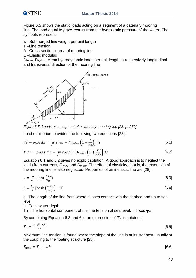
Master Thesis 2014

43

Figure 6.5 shows the static loads acting on a segment of a catenary mooring line. The load equal to ρgzA results from the hydrostatic pressure of the water. The symbols represent:

w –Submerged line weight per unit length T –Line tension A –Cross-sectional area of mooring line E –Elastic modulus Dhydro, Fhydro –Mean hydrodynamic loads per unit length in respectively longitudinal and transversal direction of the mooring line

Figure 6.5: Loads on a segment of a catenary mooring line [28, p. 259]

Load equilibrium provides the following two equations [28]:

𝑑𝑇 − 𝜌𝑔𝐴 𝑑𝑧 = [𝑤 𝑠𝑖𝑛𝜑 − 𝐹ℎ𝑦𝑑𝑟𝑜 (1 +𝑇

𝐴𝐸)] 𝑑𝑠 [6.1]

𝑇 𝑑𝜑 − 𝜌𝑔𝐴𝑧 𝑑𝜑 = [𝑤 𝑐𝑜𝑠𝜑 + 𝐷ℎ𝑦𝑑𝑟𝑜 (1 +𝑇

𝐴𝐸)] 𝑑𝑠 [6.2]

Equation 6.1 and 6.2 gives no explicit solution. A good approach is to neglect the loads from currents, Fhydro and Dhydro. The effect of elasticity, that is, the extension of the mooring line, is also neglected. Properties of an inelastic line are [28]:

𝑠 =𝑇𝐻

𝑤 sinh (

𝑤 𝑥𝐻

𝑁𝐻) [6.3]

ℎ =𝑇𝐻

𝑤[cosh (

𝑤 𝑥𝐻

𝑁𝐻) − 1] [6.4]

s –The length of the line from where it loses contact with the seabed and up to sea level h –Total water depth TH –The horizontal component of the line tension at sea level, = T cos φw

By combining Equation 6.3 and 6.4, an expression of TH is obtained:

𝑇𝐻 =𝑤 (𝑠2−ℎ2)

2 ℎ [6.5]

Maximum line tension is found where the slope of the line is at its steepest, usually at the coupling to the floating structure [28]:

𝑇𝑚𝑎𝑥 = 𝑇𝐻 + 𝑤ℎ [6.6]

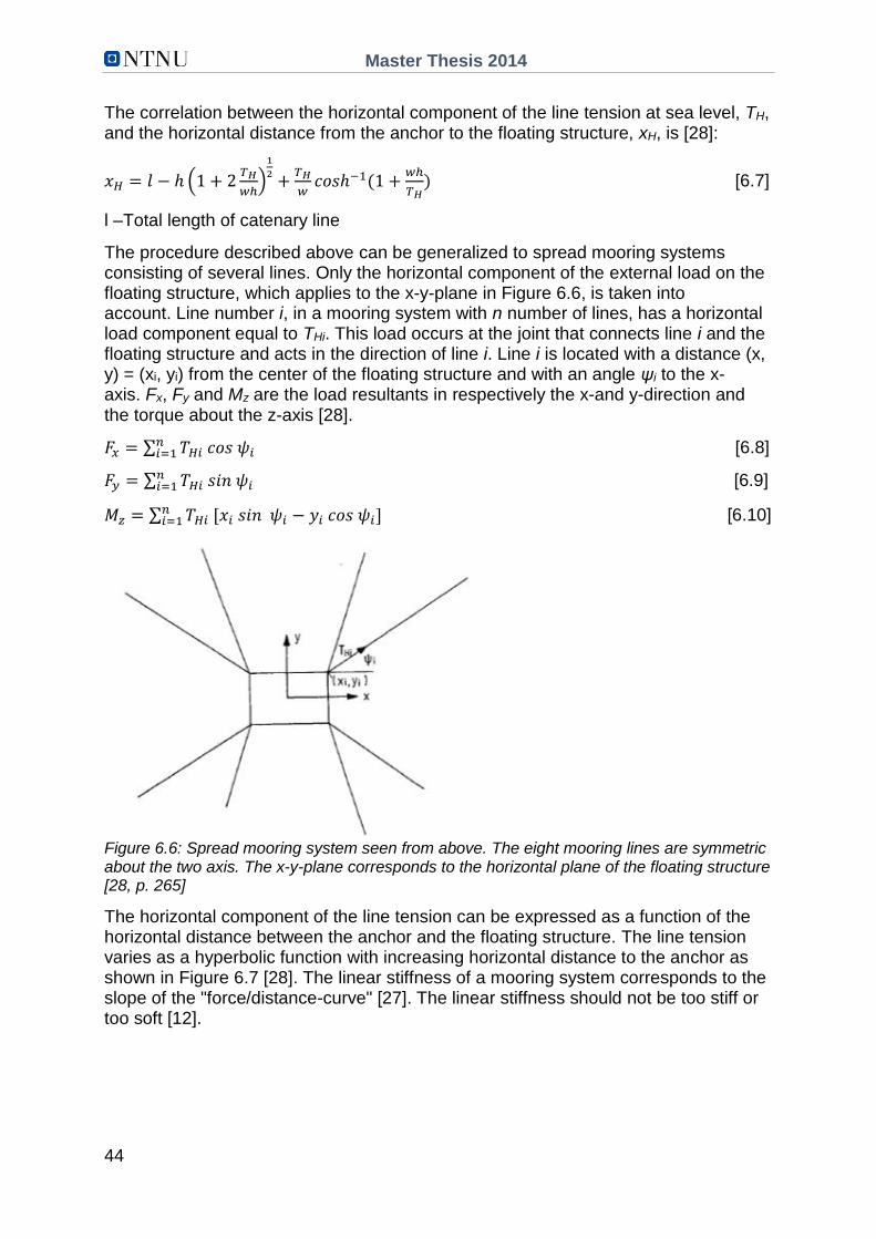
Master Thesis 2014

44

The correlation between the horizontal component of the line tension at sea level, TH, and the horizontal distance from the anchor to the floating structure, xH, is [28]:

𝑥𝐻 = 𝑙 − ℎ (1 + 2𝑇𝐻

𝑤ℎ)

1

2+

𝑇𝐻

𝑤𝑐𝑜𝑠ℎ−1(1 +

𝑤ℎ

𝑇𝐻) [6.7]

l –Total length of catenary line

The procedure described above can be generalized to spread mooring systems consisting of several lines. Only the horizontal component of the external load on the floating structure, which applies to the x-y-plane in Figure 6.6, is taken into account. Line number i, in a mooring system with n number of lines, has a horizontal load component equal to THi. This load occurs at the joint that connects line i and the floating structure and acts in the direction of line i. Line i is located with a distance (x, y) = (xi, yi) from the center of the floating structure and with an angle ψi to the x-axis. Fx, Fy and Mz are the load resultants in respectively the x-and y-direction and the torque about the z-axis [28].

𝐹𝑥 = ∑ 𝑇𝐻𝑖 𝑐𝑜𝑠 𝜓𝑖𝑛𝑖=1 [6.8]

𝐹𝑦 = ∑ 𝑇𝐻𝑖 𝑠𝑖𝑛 𝜓𝑖𝑛𝑖=1 [6.9]

𝑀𝑧 = ∑ 𝑇𝐻𝑖 [𝑥𝑖 𝑠𝑖𝑛 𝜓𝑖 − 𝑦𝑖 𝑐𝑜𝑠 𝜓𝑖]𝑛𝑖=1 [6.10]

Figure 6.6: Spread mooring system seen from above. The eight mooring lines are symmetric about the two axis. The x-y-plane corresponds to the horizontal plane of the floating structure [28, p. 265]

The horizontal component of the line tension can be expressed as a function of the horizontal distance between the anchor and the floating structure. The line tension varies as a hyperbolic function with increasing horizontal distance to the anchor as shown in Figure 6.7 [28]. The linear stiffness of a mooring system corresponds to the slope of the "force/distance-curve" [27]. The linear stiffness should not be too stiff or too soft [12].

Master Thesis 2014

45

Figure 6.7: Force/distance-curve. The horizontal tensile load in the mooring line is a function of the horizontal distance to the anchor. TH is the horizontal component of the line load. TH arises from environmental loads on the floating structure. XH is the horizontal distance between the anchor and the floating structure. Here, the water depth is h = 25 m, the weight of the chain in water is w = 828 N/m and the chain length is l = 100 m [28, p. 263]

The equation of motion in a static system can be expressed as [27]:

𝑘 𝑥 = 𝐹𝑥(𝑡) [6.11]

k –Linear stiffness x –Horizontal displacement Fx(t) –Time dependent horizontal external load in the direction of the displacement

When exposed to the design load, the lines have to lie with their lower end on the seabed not causing vertical loading on the anchor [27]. Maximum line tension should, with sufficient accuracy, not exceed the minimum breaking load provided by the manufacturer. If the tensile load is too large, the length of the lines, the number of lines, the material properties or the lines pretension will change. Calculations are repeated until adequate safety is achieved. In addition to calculations in the ultimate limit state, calculations in the accidental limit state must be carried out. This is done by assuming that the most loaded line fails and that the remaining lines must carry the external loading.

Quasi-static and dynamic analysis are more accurate, but also more time consuming than static analysis. In such analysis, the equation of motion is usually non-linear and the effects of mass and damping are taken into account. The equation of motion is [27]:

(𝑚 + 𝐴𝑚𝑎𝑠𝑠)�� + 𝐶�� + 𝐶𝑉��|��| + 𝑘𝑥 = 𝐹𝑥(𝑡) [6.12]

m –Mass of the floating structure Amass –Added mass C –Linear damping CV –Viscous damping k –Stiffness x –Displacement (in each degree of freedom) Fx(t) – Time dependent horizontal external load in the direction of the displacement

Master Thesis 2014

46

Quasi-static analysis is suitable when determining mooring line response due to static loads and approximately static loads, such as mean environmental loads and loads due to low-frequency motions of the structure [23]. Dynamic analysis is used to determine mooring line response due to wave frequency motions of the structure and the mooring line itself. In a dynamic analysis, the dynamic response of the lines and their influence on the floating structure is considered. Loads like hydrodynamic damping and inertia forces are all included in the equation of motion.

Master Thesis 2014

47

CHAPTER 7

Failure of Mooring Systems

A long-term mooring system is supposed to withstand the design load at the end of

its service life. This means that the mooring system has to withstand a 100-year

storm after approximately 20 years of wear, fatigue and corrosion [12].

Figure 7.1 illustrates some of the main factors that affect a mooring system's service

life. Bending occurs at abrupt changes of the slope of the mooring line and the

largest line tension occurs where the slope is at its steepest. Most of the cyclic

movements occur in the so-called thrash zone, at the end of the catenary line where

the chain comes in contact with the seabed [12]. The chain is exposed to abrasion

and surface damage due to movements in this thrash zone. If the chain is studded,

another problem arises: the stud may loosen and move freely in the link. If so, the

end of the stud and the side of the link are particularly exposed to corrosion.

Figure 7.1: Wear, fatigue and corrosion of a catenary mooring line [12, p. 65]

7.1 Causes of Mooring Line Failure

Overload may lead to plastic deformations, yielding and ductile failure. On the other

hand, cyclic axial load, cyclic bending and/or cyclic torsion of non-critical size may

lead to crack propagation and brittle failure. Cyclic loading as well as changes in

geometry may cause high stresses and crack propagation. Plastic deformations due

to proof loading or overload and notches or surface damages due to wear or

corrosion will lead to changes in the cross-sectional geometry. Sometimes these

geometric changes give unexpected effects.

7.1.1 Out of Plane Bending

When the line tension increases, it will become more and more difficult to obtain a

rotation between successive links [26]. A rolling mechanism would still be possible

even for high pretensions if the surfaces of the links were perfectly cylindrical. Small

Master Thesis 2014

48

out of plane bending stresses occur when links rotate freely. According to Offshore

Technology Conference paper 17238 [26], these stresses are normally not harmful:

"Unlike a rod, a chain can be piled or laid in any shape and thus we tend to think that

a chain does not have a bending stiffness. In most cases the tension in a chain is so

low that the links can roll or slide on each other to accommodate the rotations

imposed at the ends of the chain by the floating body [26, p. 2]."

The severe out of plane bending stresses occur when the surface of contact between

two links is permanently deformed, typically due to proof loading [26]. Then the links

possess a locking mode, an interlink friction force that prevent the links from rolling.

This friction provides bending stiffness to the chain and drastic changes in the stress

distribution. If a rotation is imposed on one chain link, the complete chain will have to

bend. The stresses generated by this bending are high and located at the surface of

the contact area between links. Rotations due to roll and pitch of the floating structure

will result in high stresses when the links are locked and not free to rotate relative to

each other. The upper end of the chain is especially exposed to cyclic bending and

failure.

Figure 7.2 shows bending of a chain link out of its "main plane" when a rotation αtotal

is imposed on the chain end and the links cannot roll on each other.

Figure 7.2: Out of plane bending of chain links, links are locked at the surface of contact [26,

p. 4]

7.1.2 Torsion

A chain that is straight and subjected to an axial load does not twist or generate any

torque [30]. However, if a chain is twisted while carrying axial load, it behaves in a

highly non-linear manner. The magnitude of the torque depends on the level of twist

and the axial load.

Typical mooring lines include wire or fiber rope in combination with chain, and while

the chain is torque balanced, the other components may not be. The wire or fiber

rope may try to twist the chain when the mooring line is subjected to axial loading

[30]. Secondly, a chain may be installed with a twist or twist during service. Even

though the mooring line is handled with care, it may be difficult to avoid twisting

during installation of a long chain.

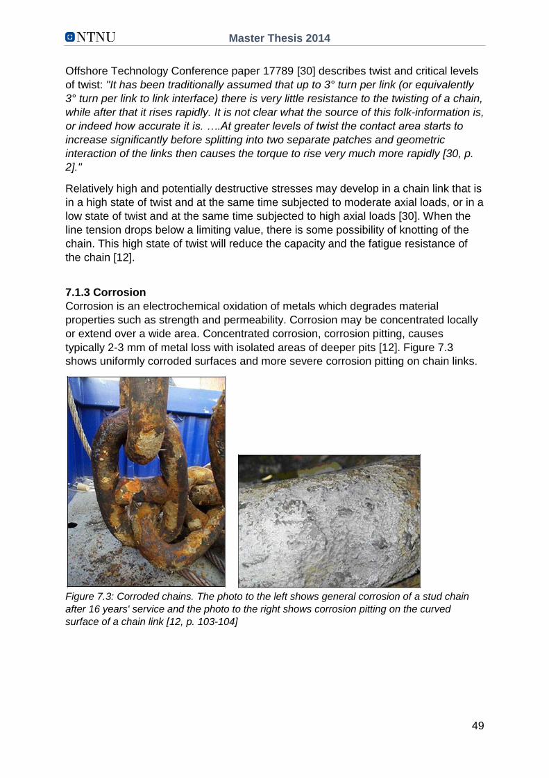
Master Thesis 2014

49

Offshore Technology Conference paper 17789 [30] describes twist and critical levels

of twist: "It has been traditionally assumed that up to 3° turn per link (or equivalently

3° turn per link to link interface) there is very little resistance to the twisting of a chain,

while after that it rises rapidly. It is not clear what the source of this folk-information is,

or indeed how accurate it is. ….At greater levels of twist the contact area starts to

increase significantly before splitting into two separate patches and geometric

interaction of the links then causes the torque to rise very much more rapidly [30, p.

2]."

Relatively high and potentially destructive stresses may develop in a chain link that is

in a high state of twist and at the same time subjected to moderate axial loads, or in a

low state of twist and at the same time subjected to high axial loads [30]. When the

line tension drops below a limiting value, there is some possibility of knotting of the

chain. This high state of twist will reduce the capacity and the fatigue resistance of

the chain [12].

7.1.3 Corrosion

Corrosion is an electrochemical oxidation of metals which degrades material

properties such as strength and permeability. Corrosion may be concentrated locally

or extend over a wide area. Concentrated corrosion, corrosion pitting, causes

typically 2-3 mm of metal loss with isolated areas of deeper pits [12]. Figure 7.3

shows uniformly corroded surfaces and more severe corrosion pitting on chain links.

Figure 7.3: Corroded chains. The photo to the left shows general corrosion of a stud chain

after 16 years' service and the photo to the right shows corrosion pitting on the curved

surface of a chain link [12, p. 103-104]

Master Thesis 2014

50

The following factors will influence the corrosion rate [12]:

- Dissolved oxygen

- Temperature

- Salinity

- Velocity of water particles

- Sulphate reducing bacterial count

These factors do all, to some degree, depend on geographical location [12]. The

oxygen content is influenced mainly by water particle velocity and water temperature.

The temperature drops and the salinity rise with increasing water depth. The oxygen

content is high near sea level and in very deep water due to high particle velocity at

sea level and low temperatures in deep water. This is an undesirable effect from a

corrosion perspective.

Sulphate reducing bacteria (SRB) may cause corrosion pitting and rapid damage to

mooring systems in the North Sea, south-east Asia and off Brazil [12]. SRB are

anaerobic and can develop in slime layers with thickness less than 1 mm. These

bacteria can cause severe corrosion by accelerating the reduction of sulphate

compounds to corrosive hydrogen sulphide. Standard bacteria cultivation tests are

used to check the amount of SRB. In general, 1 SRB per liter sea water is fairly

normal and even higher concentrations can be found in the top soil of the seabed.

Protection against chain corrosion and wear is normally provided by increasing the

chain diameter [12]. Normal practice is to increase the chain diameter by 0.2 mm to

0.4 mm per service year. Recommended corrosion allowance is given in Table 7.1 for

mooring lines in the splash zone, thrash zone and elsewhere on a catenary line.

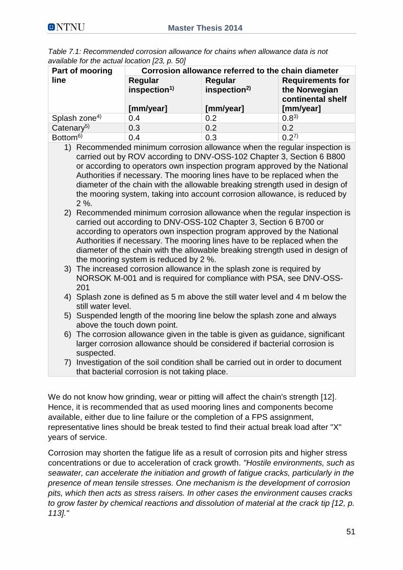
Master Thesis 2014

51

Table 7.1: Recommended corrosion allowance for chains when allowance data is not

available for the actual location [23, p. 50]

Part of mooring line

Corrosion allowance referred to the chain diameter

Regular inspection1) [mm/year]

Regular inspection2) [mm/year]

Requirements for the Norwegian continental shelf [mm/year]

Splash zone4) 0.4 0.2 0.83)

Catenary5) 0.3 0.2 0.2

Bottom6) 0.4 0.3 0.27)

1) Recommended minimum corrosion allowance when the regular inspection is carried out by ROV according to DNV-OSS-102 Chapter 3, Section 6 B800 or according to operators own inspection program approved by the National Authorities if necessary. The mooring lines have to be replaced when the diameter of the chain with the allowable breaking strength used in design of the mooring system, taking into account corrosion allowance, is reduced by 2 %.

2) Recommended minimum corrosion allowance when the regular inspection is carried out according to DNV-OSS-102 Chapter 3, Section 6 B700 or according to operators own inspection program approved by the National Authorities if necessary. The mooring lines have to be replaced when the diameter of the chain with the allowable breaking strength used in design of the mooring system is reduced by 2 %.

3) The increased corrosion allowance in the splash zone is required by NORSOK M-001 and is required for compliance with PSA, see DNV-OSS-201

4) Splash zone is defined as 5 m above the still water level and 4 m below the still water level.

5) Suspended length of the mooring line below the splash zone and always above the touch down point.

6) The corrosion allowance given in the table is given as guidance, significant larger corrosion allowance should be considered if bacterial corrosion is suspected.

7) Investigation of the soil condition shall be carried out in order to document that bacterial corrosion is not taking place.

We do not know how grinding, wear or pitting will affect the chain's strength [12].

Hence, it is recommended that as used mooring lines and components become

available, either due to line failure or the completion of a FPS assignment,

representative lines should be break tested to find their actual break load after "X"

years of service.

Corrosion may shorten the fatigue life as a result of corrosion pits and higher stress

concentrations or due to acceleration of crack growth. "Hostile environments, such as

seawater, can accelerate the initiation and growth of fatigue cracks, particularly in the

presence of mean tensile stresses. One mechanism is the development of corrosion

pits, which then acts as stress raisers. In other cases the environment causes cracks

to grow faster by chemical reactions and dissolution of material at the crack tip [12, p.

113]."

Master Thesis 2014

52

7.1.4 Wear

Wear is a process that gradual removes material at contact surfaces in relative

motion. This process involves material properties, forces, sliding distances,

lubrication and environmental factors [12]. Wear results in increased contact area

between links while the cross-sectional area is decreases.

Archard's law provides the volume of material removed by wear [31]:

𝑣 =𝐾𝑃𝑑

𝐻 [7.1]

v –Volume of material removed

K –Wear coefficient (non-dimensional)

P –Applied load

d –Sliding distance

H –Penetration hardness

OTC paper 4764 [31] study wear and its influence on mooring line failure. The

experimental setup consisted of one fixed cylinder with a crossed cylinder on top.

The crossed cylinder rotated with an oscillatory motion through an angle while a large

compressive load was imposed. The crossed cylinder wear tests showed that the test

bars had high initial wear rates, followed by a distinct knee and a nearly linear lower

rate after approximately 150 cycles. The knee was probably caused by the

decreased contact pressure and reduced sliding distance resulting from wear. The

presence of seawater, which provided lubrication, caused a distinct reduction in wear.

7.2 Consequences of Mooring Line Failure

A mooring system is designed to withstand one line failure without further damage of

the remaining mooring lines. However, the safety factors on the remaining lines

should be raised until it has been determined with reasonable confidence why the

original line failed. Figure 7.5 shows a potential failure scenario of one mooring line.

Master Thesis 2014

53

Figure 7.4: Potential failure scenario when one single line fails [12, p. 78]

If several mooring lines fail, the remaining lines are overloaded, resulting in loss of

position of the floating structure [12].

The following factors increase the likelihood of multiple line failure [12]:

- Design: The presence of a systematic weakness in the mooring system will

apply to all lines

- Age: Fatigue, corrosion and wear will tend to deteriorate all mooring lines,

particularly in the same quadrant, to roughly the same extent over time.

- Detection: Where no line tension or equivalent monitoring system is available,

failure of a single line may go undetected. This may expose the remaining

lines to larger loads for an extended period.

Figure 7.6 shows a potential multiple line failure scenario.

Deterioration: The progressive deterioration of a component of the system under fatigue, corrosion and wear.

Failure: Followed by failure of the component under moderate storm conditions.

Detection: Line loss might be detected through tension monitoring equipment where that is installed. It is possible that the line failure could be undetected until a routine subsea check of the mooring system.

Shutdown: The system is likely to be shutdown until the continued integrity of the mooring system has been verified and new operating limits defined.

Inspection: The mooring and production systems would be inspected to identify any related damage.

Reduced operations: Resumption of operations under reduced weather criteria.

Repair: Reinstatement of the full mooring system.

Master Thesis 2014

54

Figure 7.5: Potential failure scenario when multiple lines fail [12, p. 80]

The consequences of line failure are numerous and severe. Failure in one or several

lines may lead to loss of station and:

- Subsea damage

- Damage to risers

- Pollution damage

- Capsizing

- Collision with neighboring facilities

- Loss of life

- Economical loss

- Reputation damage

7.3 Damage Statistics

HSE Research Report 444 [12] summarize line failure statistics for different floating

units in the North Sea covering the period 1980 to 2001. Table 7.2 shows that the

probability of line failure per operating year is relatively high. In the North Sea, there

are statutory requirements for mooring incidents to be reported to the UK Health and

Safety Executive (HSE). Thus, Table 7.2 gives a good indication of actual line failure

statistics.

Table 7.2: North Sea mooring line failure data from 1980 to 2001 [12, p. 12]

Type of unit Number of operating years per failure

Drilling semi-submersible 4.7

Production semi-submersible 9.0

FPSO 8.8

Deterioration: The progressive deterioration of a component of the system under fatigue, corrosion and wear.

First failure: Followed by failure of the component under moderate storm conditions. This could go undetected.

Unzipping: Overload of adjacent lines, perhaps after further deterioration if the initial failure was undetected.

Excursion: Loss of integrity of the mooring system could be identified from the loss of station keeping after failure of several lines.

Shutdown: The risers should be de-pressurized and isolated prior to damaging distortions in the system.

Master Thesis 2014

55

It is vital to detect a line failure promptly or else there is a danger of multiple line

failures and loss of station keeping.

The following data for North Sea turret moored FPSOs was collected in HSE

Research Report 444 [12]:

- 50 % of the units cannot adjust line lengths

- 33 % of the units cannot measure offsets from the equilibrium position

- 50 % of the units cannot monitor line tensions in real time

- 78 % of the units don't have line failure alarms

- 67 % of the units don't have mooring line spares available

- 87 % of the units don't have repair procedures

These data show that a line failure could be undetected due to lack of monitoring

equipment. The broken line might not be detected until a routine subsea check of the

mooring system is carried out.

However, if a line failure is detected, it may take several months to repair the

damage. Procuring new components takes time and it is recommended that

components which can be obtained at short notice from marine equipment rental

companies are available [12].

Master Thesis 2014

56

CHAPTER 8

Fatigue

Fatigue is a long-term degradation process. The process accumulate damage in

materials undergoing fluctuating loading, eventually resulting in failure even though

the maximum load is well below the elastic limit of the material [32]. Fatigue of a

material result in crack growth and local strength reduction after a sufficient number

of fluctuations.

The word "long-term mooring" is specified in DNV-OS-E301 [23] as a mooring

system that is positioned at the same location for five years or more.

8.1 The Fatigue Process

There are three stages in a fatigue process: crack initiation, propagation of one

dominant crack and final fracture [32]. The fatigue damage develops slowly in the

early stages and accelerates very quickly towards the end. The crack initiation phase

may occupy more than 95 % of the life of a smooth and mildly notched component

subjected to moderate loading. This first stage of a fatigue process usually results in

a number of micro-cracks that grow more or less independently until one crack

becomes dominant through a coalescence process as the micro-cracks start to

interact. The dominant crack grows slowly under steady fatigue loading, but starts to

accelerate when the reduction of the cross section increases the local stress field

near the crack tip, see chapter 3.3. Final fracture occurs when the remaining area is

too small to support the load.

The crack length is a simple measure of fatigue damage, but since the crack length is

small at an early stage of the fatigue process, it is easily measurable only at a

relatively late stage in the life of a component [32]. Any stress concentration in form

of external or internal surface flaws can reduce the fatigue life, particularly when the

initiation phase occupies a significant percentage of the total life. Typically, a part

with smooth and polished surface has higher fatigue strength than one with rough

surface.

Master Thesis 2014

57

The fatigue process can in many cases be

related to distinctive features of the fracture

surface of ductile components that have failed

under fluctuating loads [32]. A characteristic

feature of the fracture surface is the flat and

smooth area that possesses beach marks. This

area represents the portion of the fracture surface

over which the crack grew in a stable, slow mode.

The rougher regions, showing plastic

deformation, is the final fracture area where the

crack progressed in an unstable mode. The

beach marks form concentric rings radially about

the location of the crack initiation. This is shown in

Figure 8.1. The size of the slow-growth regions Figure 8.1: Beach marks on a

and the final fracture regions give an indication of the fatigue fracture surface. The

maximum stresses and fracture toughness of the crack originates from the

material. A large final fracture area for a given center of the rings. Taken

material indicates high loading, whereas a small from Fontenot W, Zhang L.

area indicates that the load was smaller at fracture. 76 mm Chain Link Fatigue

Similarly, for a fixed maximum stress, the area Failure. SOFEC Inc., Stress

corresponding to slow crack growth increases Engineering Services Inc.

with the fracture toughness of the material. Beach [undated; 27.04.2014]

marks are formed when the crack grows

intermittently and at different rates during random

variations of the loading pattern. Thus, these marks are not observed on the surface

of fatigue specimens tested under constant amplitude loading conditions.

The average crack growth is a few millimeters per million cycles in high cycle fatigue

[32]. DNV-RP-C203 [22] describes low cycle and high cycle fatigue as follows: "By

fatigue strength assessment of offshore structure is normally understood capacity

due to high cycle fatigue loading. By high cycle loading is normally understood cycles

more than 10 000. For example stress response from wave action shows typically 5

million cycles a year. A fatigue assessment of response that is associated with

number of cycles less than 10 000 is denoted low cycle fatigue [22, p. 121]."

Low cycle fatigue is associated with localized plastic behavior in metals. Strain is a

more meaningful and more easily measurable parameter than stress when it comes

to plastic behavior [32]. Thus, low cycle fatigue life is related to strains while high

cycle fatigue life is related to stresses. The following chapters will focus on high cycle

fatigue.

8.2 Fatigue Stress and Fatigue Life

The sinusoidal or constant amplitude stress-time history is the simplest

representation of stress spectrum [32]. The mean load and thus the mean stress is

constant in a constant amplitude stress spectrum. Since the loading history is easily

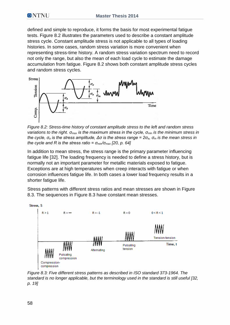
Master Thesis 2014

58

defined and simple to reproduce, it forms the basis for most experimental fatigue

tests. Figure 8.2 illustrates the parameters used to describe a constant amplitude

stress cycle. Constant amplitude stress is not applicable to all types of loading

histories. In some cases, random stress variation is more convenient when

representing stress-time history. A random stress variation spectrum need to record

not only the range, but also the mean of each load cycle to estimate the damage

accumulation from fatigue. Figure 8.2 shows both constant amplitude stress cycles

and random stress cycles.

Figure 8.2: Stress-time history of constant amplitude stress to the left and random stress

variations to the right. σmax is the maximum stress in the cycle, σmin is the minimum stress in

the cycle, σa is the stress amplitude, Δσ is the stress range = 2σa, σm is the mean stress in

the cycle and R is the stress ratio = σmin/σmax [20, p. 64]

In addition to mean stress, the stress range is the primary parameter influencing

fatigue life [32]. The loading frequency is needed to define a stress history, but is

normally not an important parameter for metallic materials exposed to fatigue.

Exceptions are at high temperatures when creep interacts with fatigue or when

corrosion influences fatigue life. In both cases a lower load frequency results in a

shorter fatigue life.

Stress patterns with different stress ratios and mean stresses are shown in Figure

8.3. The sequences in Figure 8.3 have constant mean stresses.

Figure 8.3: Five different stress patterns as described in ISO standard 373-1964. The

standard is no longer applicable, but the terminology used in the standard is still useful [32,

p. 19]

Master Thesis 2014

59

The fatigue life is typically expressed in terms of cycles to failure [32]. The total

fatigue life is the sum of number of cycles in the initiation stage and the propagation

stage:

𝑁𝑡 = 𝑁𝑖 + 𝑁𝑝 [8.1]

Nt –Total number of cycles

Ni –Number of cycles in the initiation stage

Np –Number of cycles in the propagation stage

Fatigue data are usually presented as S-N-curves [32]. The applied stress range S is

plotted against total cycles to failure N (Nt) and as the stress range decreases,

number of cycles to failure increases. Most metals except for aluminum and

nonferrous alloys have a "knee-point" on the S-N-curve from which the curve

proceeds horizontally. Failure does not occur when the stress range is smaller than

this limit called the fatigue limit or the endurance limit. All materials, however, exhibit

a relatively flat curve in the high cycle region where number of cycles exceeds

about 105.

8.3 Fatigue Analysis Based on S-N-data

Fatigue design is based on use of S-N-curves which are obtained from fatigue tests.

A characteristic feature of fatigue tests is the large scatter in test results. This is

especially evident when a number of specimens of a specific material are tested at

the same stress level. S-N-curves should be on the safe side with lower band values

based on large scale fatigue testing. The S-N-curves in DNV-RP-C203 [22] are

based on the mean value minus two times the standard deviation for relevant

experimental data. The S-N-curves are thus associated with a 97.7 % probability that

failure do not occur.

The basic design S-N-curve is given as [22]:

log(𝑁𝑡) = log(��) − 𝑚 𝑙𝑜𝑔(∆𝜎) [8.2]

Nt –Number of cycles to failure for stress range Δσ

Δσ –Stress range

m –Negative inverse slope of the design S-N-curve

ā –Intercept of the design S-N-curve with the log(N) axis

The design S-N-curve in Figure 8.4 is taken from DNV-OS-E301 [23]. The S-N-curve

is valid for stud chains and studless chains exposed to free corrosion. In the case of

chain tests in air, the effect of seawater shall be accounted for by a reduction of the

fatigue life by 2 for stud chains and by a factor of 5 for studless chains [23]. The S-N-

curves are based on nominal stress range. The nominal stress range in a chain link is

equal to the external tensile load divided by the nominal cross-sectional area:

N/2π(D2/4), where D is the nominal cross-sectional diameter and N is the external

tensile load.

Master Thesis 2014

60

Figure 8.4: S-N-curves for different mooring components. The S-N-curves are applicable for

tension-tension stresses. The chains are exposed to free corrosion in seawater while the

steel wire ropes are protected from the corrosive effect of seawater. Parameters for the

constant slope S-N-curves are listed to the right [23, p. 51-52]

The S-N-curve in Figure 8.4 does not distinguish between steel grades. However,

API RP 2SK [33] provides T-N-curves for different mooring components subjected to

axial tensile loading. The T-N-curve take steel grade into account by introducing a

ratio of tension range to minimum breaking load.

The design T-N-curve is given as [33]:

𝑁𝑡𝑅𝑀 = 𝐾 [8.3]

Nt –Number of cycles to failure

R –Ratio of tension range to minimum breaking load for steel grade R3, R4 or R4S,

= ∆T/MBL

M,K –Factors

The T-N-curve in Figure 8.5 is taken from API RP 2SK [33]. It does not say if it is

applicable to chains exposed to free corrosion or chains with cathodic protection.

However, it recommends use of a safety factor of 3 to yield fatigue designs with

acceptable probability of failure, meaning that the predicted mooring component

fatigue life shall be at least three times the design service life of the mooring system.

Parameter ā m

Stud chain 1.2·1011 3.0

Studless chain

6.0·1010 3.0

Stranded rope

3.4·1014 4.0

Spiral rope 1.7·1017 4.8

Master Thesis 2014

61

Figure 8.5: T-N-curves for different mooring components. The steel wire ropes are protected

from the corrosive effect of seawater. Parameters for the constant slope T-N-curves are

listed to the right [33, p. 26]

There are in general three types of environmental conditions that influence S-N-

curves. Fatigue tests that form the basis for S-N-curves are carried out in air, in

seawater without corrosion protection or in seawater with corrosion protection. S-N-

charts shall state the corresponding environmental condition under which the fatigue

testing is conducted. Figure 8.6 shows S-N-curves for specimens tested in air, in

seawater with cathodic protection and in seawater without cathodic protection. The

specimens tested in air has, not surprisingly, a longer fatigue life than the specimens

tested in seawater when exposed to the same fatigue loading. The S-N-curve for

seawater with cathodic protection is close to the curve for seawater without cathodic

protection at low number of cycles and moves towards the curve for air when number

of cycles increase. When number of cycles is large enough, the two curves coincide.

Figure 8.6: Example of S-N-curves for identical test pieces tested in air, in seawater with

cathodic protection and in seawater without cathodic protection [34]

Parameter M K

Stud chain 3.0 1000.00

Studless chain

3.0 316.00

Connecting link

3.0 178.00

Stranded rope

4.09 10(3.20-

2.79Lm)

Spiral rope 5.05 10(3.25-

3.43Lm)

Master Thesis 2014

62

In addition to environmental conditions there are three possible states of stress

ranges that S-N-curves can relate to. Figure 8.7 shows the three types of stresses.

The nominal stress range is uniform over the cross-sectional area, thus easy to

calculate. However, the hot spot stress and the notch stress vary typically linearly

and hyperbolic over the cross-sectional area with maximum values at the material

surface. The stress range is smallest in the case of nominal stresses, it increase for

hot spot stresses and is largest for notch stresses. Figure 8.7 shows hot spot

stresses and notch stresses at a weld toe, but these types of stresses may also

appear elsewhere in a structure. Hot spot stress is understood to be the geometric

stress created by the considered detail, while the notch stress is defined as the total

stress resulting from the geometry of the detail and the non-linear stress field due to

notches [22]. Note that the S-N-curves for the different stress states are parallel. By

multiplying the nominal stress range with the relevant stress concentration factor, one

obtain the hot spot stress range or the notch stress range.

Figure 8.7: Three states of stresses. The upper figure shows stress distributions over the

cross-sectional area at a weld toe. The S-N-curves for nominal stress, hot spot stress and

notch stress are parallel and therefore proportional to each other. The k-factor is the stress

concentration factor due to abrupt changes in geometry [34]

8.3.1 Fatigue Damage

The fatigue life may be calculated based on the assumption of linear cumulative

damage using S-N-data [22]. The so-called Palmgren-Miner rule is a widely used

fatigue criterion summing up the damage done by different constant stress ranges,

∆σi, each with ni number of repetitions, and given by:

𝐷𝑎𝑐𝑐. = ∑𝑛𝑖

𝑁𝑡𝑖

𝑘𝑡𝑖=1 =

1

ā∑ 𝑛𝑖

𝑘𝑖=1 (∆𝜎𝑖)

𝑚 ≤ 𝜂 [8.4]

Dacc. –Accumulated fatigue damage

ā –Intercept of the design S-N-curve with the log(N) axis

m –Negative inverse slope of the design S-N-curve

kt –Number of stress blocks (environmental state)

ni –Number of stress cycles in stress block i

Master Thesis 2014

63

Nti –Number of cycles to failure at constant stress range ∆σi

η –Usage factor < 1.0, = 1/Design fatigue factor from DNV-OS-C101, section 6

Figure 8.8 illustrates the procedure when using Palmgren-Miner rule. Stress ranges

are used in combination with the corresponding S-N-curve to find number of cycles to

failure for each constant stress range. Number of constant stress ranges must be

large enough to ensure reasonable numerical accuracy, and shall not be less than 20

[22].

Figure 8.8: Fatigue damage accumulation, showing two constant stress ranges [34]

Offshore structures are subjected to a number of different loading conditions and

stress ranges. DNV-OS-E301 [23] describes fatigue analysis of offshore structures:

"The long-term environment can be represented by a number of discrete conditions.

Each condition consists of a reference direction and a reference sea state

characterized by a significant wave height, peak period, current velocity and wind

velocity. The probability of occurrence of these conditions must be specified. In

general 8 to 12 reference directions provide a good representation of the directional

distribution of a long-term environment. The required number of reference sea states

can be in the range of 10 to 50. Fatigue damage prediction can be sensitive to the

number of sea states, and sensitivity studies can be necessary [23, p. 52]."

8.3.2 Mean Stress Effects

The stress range is the most important parameter of fatigue life, but the mean stress

plays an important role too. In general, a tensile mean stress reduces the fatigue life

while a compressive mean stress increases the fatigue life due to a mean stress

equal to zero [32].

The effect of mean stress on the fatigue strength is commonly presented in Haigh

diagrams as shown in Figure 8.9. The mean stress has more effect in notched parts

than on smooth parts. The test results in Figure 8.9 are obtained for small unnotched

specimens, tested at various tensile mean stresses. The straight lines are the

modified Goodman and the Soderberg lines, and the curved line is the Gerber

parabola.

Master Thesis 2014

64

Figure 8.9: Haigh diagram. Sa/Sf is plotted against Sm/Su. Sa is the limiting value of σa, Sm is

the limiting value of σm, Su is the limiting ultimate tensile strength and Sf is the unnotched fully

reversed fatigue limit or the fatigue strength at about 106 to 108 cycles [32]

The three relations in the Haigh diagram are empirical and represented by the

following equations [32]:

Modified Goodman: 𝑆𝑎

𝑆𝑒+

𝑆𝑚

𝑆𝑢= 1 [8.5]

Gerber: 𝑆𝑎

𝑆𝑒+ (

𝑆𝑚

𝑆𝑢)2 = 1 [8.6]

Soderberg: 𝑆𝑎

𝑆𝑒+

𝑆𝑚

𝑆𝑦= 1 [8.7]

Sa – Limiting value of alternating stress amplitude, σa

Sm – Limiting value of mean stress, σm

Su – Limiting value of tensile strength, fu

Sy –Limiting value of yield stress, fy

Se – Endurance limit or fatigue limit, given by [35]:

𝑆𝑒 = 𝑘𝑎𝑘𝑏𝑘𝑐𝑘𝑑𝑘𝑒𝑆′𝑒 [8.8]

ka –Surface condition modification factor

kb – Size modification factor (deterministic)

kc – Load modification factor

kd –Temperature modification factor

ke – Miscellaneous-effects modification factor

S'e –Rotating beam test endurance limit, = 0.504 Su, Su ≤ 1460 MPa

Some of the test results in the Haigh diagram fall below the Gerber line, i.e. the line is

not conservative. The Goodman line represent a lower limit of data while the

Soderberg line is a relatively conservative lower bound.

The fatigue life can be calculated as follows [35]:

Master Thesis 2014

65

𝑁𝑡 = (𝑆𝑓

𝑎)1/𝑏 [8.9]

Sf –Unnotched fully reversed fatigue limit or the fatigue strength at about 106 to 108

cycles

a, b –Factors

𝑆𝑓 = {

𝜎𝑎

1−(𝜎𝑚/𝑆𝑢) ,

𝜎𝑎

1−(𝜎𝑚/𝑆𝑢)2 ,𝜎𝑎

1−(𝜎𝑚/𝑆𝑦) 𝜎𝑚 > 0

𝑆𝑒 𝜎𝑚 ≤ 0 [8.10]

𝑏 =log(

𝜎′𝐹

𝑆𝑒)

log (2𝑁𝑒)= − (

1

3) log (

𝑓 𝑆𝑢

𝑆𝑒) [8.11]

𝑎 =(𝑓 𝑆𝑢)2

𝑆𝑒 [8.12]

Ne –Endurance limit life

σ'F –Fatigue strength coefficient, = Su + 345 MPa

f –Factor, = σ'F (2000)b/Su

8.4 Fatigue Analysis Based on Fracture Mechanics

Fracture mechanics may be used for fatigue analysis as supplement to S-N-data to

define acceptable levels of defects and plan in-service inspections [22]. The purpose

of such analysis is to document, by means of calculations, that fatigue cracks, which

might occur during service life, will not exceed the crack size corresponding to

unstable fracture. The calculations shall be performed such that the structural

reliability by use of fracture mechanics will not be less than that achieved by use of

S-N-data. The fracture mechanic procedure corresponds to the crack growth stage of

the fatigue process. Since crack initiation is not included in the fracture mechanics

approach, shorter fatigue life is normally derived from fracture mechanics than by

S-N-data.

Fracture mechanics is used to evaluate the strength of a structure or a component in

the presence of a crack or flaw [20]. The initial crack size to be used in calculations

shall consider the experienced imperfection or defect size of the existing material,

weldment and geometry as well as the reliability of the inspection method [22]. If the

detail contains residual stresses, the whole stress range shall be applied. Only stress

components normal to the propagation plane need to be considered.

Figure 8.10 shows three different crack growth histories. The three tested specimens

are identical, but with different cyclic loading conditions where stress range S1 is

bigger than stress range S2 that is bigger than stress range S3. All specimens have

the same initial crack length, a0, and the same minimum stress. The crack growth

with respect to number of cycles corresponds to the slope of the curves. From Figure

8.10 we see that with higher stresses the crack growth rates are higher at a given

crack length and the fatigue crack growth life is shorter [20]. The crack lengths at

fracture are also shorter at the higher stress levels. Thus, for a given initial crack

Master Thesis 2014

66

length, the life to fracture depends on the magnitude of the applied stress range and

the fracture resistance of the material.

Figure 8.10: Fatigue crack length versus load cycles at three different stress ranges. The

initial crack length is constant and final fracture is indicated by a "x" [20, p. 143]

Crack length versus cycle curves are not applicable to fatigue design except under

exactly the same conditions used to obtain the data [20]. The fatigue crack growth

rate can be expressed as a function of the stress intensity factor range. The stress

intensity factor is derived in Chapter 3.3 and the stress intensity factor range is:

∆𝐾 = 𝐾𝑚𝑎𝑥 − 𝐾𝑚𝑖𝑛 = 𝛽𝜎𝑚𝑎𝑥 √𝜋 𝑎 − 𝛽𝜎𝑚𝑖𝑛 √𝜋 𝑎 = 𝛽∆𝜎 √𝜋 𝑎 [8.13]

β –Dimensionless factor dependent on the structures geometry and loading. Approximately equal to 1.0 σ –Nominal stress that would exist if the crack were absent. The nominal stress is normal to the crack a –Full crack length if the crack evolves from the edge or half the length if the crack occurs with a distance to the edge of the structure

Since the stress intensity factor is undefined for compressive stresses, Kmin is taken as zero if σmin is compressive.

Figure 8.11 shows a log-log plot of fatigue crack growth rate versus stress intensity

factor range. The curve has a sigmoidal shape or S-shape that can be divided into

three major regions [20]. Region 1 indicates a threshold value of the stress intensity

factor below which there is no observable crack growth. The threshold value occurs

at a crack growth rate of order 1·10-10 m/cycle or less. Below this value, fatigue

cracks are characterized as non-propagating cracks. The crack growth in region 1 is

mainly controlled by microstructure, mean stress, load frequency and environment.

Region 2 shows a linear relationshop between log(da/dN) and log(∆K). This gives the

following equation known as Paris' equation:

Master Thesis 2014

67

𝑑𝑎

𝑑𝑁= 𝐶 (∆𝐾)𝑚 [8.14]

C –Factor found by extending the straight line to ∆K = 1 MPa√m

m –Slope of the curve in region 2

Region 2 corresponds to a stable macroscopic crack growth that is typically

controlled by the environment [20]. In region 3, the fatigue crack growth rates are

very high as they approach instability. This region is controlled primarily by fracture

toughness, which in turn depends on microstructure, yield stress and environment as

described in Chapter 3.3.

Figure 8.11: Fatigue crack growth rate versus stress intensity factor range with units m/cycle

and MPa√m respectively [20, p. 144]

If one knows the stress intensity factor expression for a given component and

loading, the fatigue crack growth life of the component can be obtained by integrating

the sigmoidal curve between the limits of initial crack size and critical crack size [20].

In many cases, integration of Paris' equation by extrapolating to both regions 1 and 3

may be satisfactory, as it often gives conservative fatigue crack growth life values.

The approximate fatigue life is calculated as:

𝑁𝑡 = ∫ 𝑑𝑁𝑡𝑁

0= ∫

𝑑𝑎

𝐶(∆𝐾)𝑚

𝑎𝑐

𝑎𝑖 [8.15]

ac –Critical crack length

ai – Initial crack length

Master Thesis 2014

68

8.5 Main Factors Influencing the Fatigue Life

Imitation of real fatigue behavior is difficult because the fatigue process is complex

and influenced by many factors. That is why so many laboratory fatigue tests have

large scatter in test results. Some of the factors influencing the fatigue life are

notches, surface roughness, corrosion, weldments, mean stresses and residual

stresses [32].

For unnotched structural components the fatigue strength increase with increasing

material strength as a result of an increasing crack initiation period [32]. Structural

components that are sharply notched or subjected to severe corrosion will quickly

initiate cracks. Since the crack growth is very little influenced by material strength, the

fatigue life of notched and severe corroded components is not particularly influenced

by material strength.

The mean stress will sometimes influence the fatigue life. In general, a tensile mean

stress reduces fatigue life while a compressive mean stress increases fatigue life

[32].

Most fatigue cracks appear at the surface since slip occurs easier here than in the

interior of a material [32]. In addition, simple fracture mechanics considerations show

that surface defects and notches are much more damaging than internal defects of

similar size. Thus, the surface finish is one of the important factors influencing fatigue

life. The surface finish, expressed by average surface roughness, is a measure of

mean distance between peaks and troughs over a specified surface distance. The

effect of surface finish is determined by comparing the fatigue limit of specimens with

a given surface finish with the fatigue limit of highly polished standard specimens.

Welds are in many cases the weak link in a structural component. The weld design

will obviously lead to abrupt changes in geometry and an irregular surface finish.

Thus, stress concentrations tends to appear near welds and reduce the fatigue

strength. In addition, residual stresses from the welding process tend to occur close

to welds.

Normally stud chains have a longer fatigue life than studless chains. However,

studless chains do not have the fatigue issues associated with studs, such as loose

stud, stud weld crack, sharp corners at stud footprint, corrosion between stud and link

and defects hidden behind the stud that cannot be detected by inspection [33].

8.6 Residual Stresses

Residual stresses occur when a region of a structural component is strained beyond

the elastic limit while other regions are elastically deformed [32]. When the force

causing the deformation is removed, the elastically deformed material springs back

and impose residual stresses in the plastically deformed material. The high stresses

causing yielding arise from thermal expansion or external loading.

Master Thesis 2014

69

The residual stress is of opposite sign to the initially applied stress [32]. Therefore, if

a notched member is exposed to a tensile load until yielding occurs, the resulting

residual stresses near the notch tip are compressive. Compressive residual stresses

may increase the fatigue life. However, the stresses may relax with time and reduce

the favorable effects of residual stresses. Since the magnitude of the residual

stresses is related to the yield stress their effect on fatigue strength is stronger the

higher strength of the material.

Mooring chains are proof loaded by manufacturer before being distributed. The proof

load is based on steel grade and nominal cross-sectional diameter and is

approximately 70-80 % of minimum breaking load. The load causes yielding at

sensitive locations in the links, resulting in residual stresses after unloading. The

flash butt weld in each link is also subject to residual stresses. These stresses come

from thermal expansion during flash butt welding.

8.7 Notches

Fatigue is a weakest link process that depends on the local stress in a structural

component [32]. Strains and stresses at a notch makes no significant reduction in

strength or increase in deformation, but the cracks that may start growing at notches

eventually result in fracture. It is therefore necessary to calculate the local stress in

terms of a stress concentration factor and relate this to the fatigue behavior of the

notched component. The stress concentration factor derived in Chapter 3.5 can be

used to reduce the stress range in an S-N-curve for unnotched components to get an

S-N-curve for notched components. The predicted curve for notched components fits

experimental data reasonable well in the high cycle regions, but in the low cycle

regions, the calculated curve is far too conservative. Thus arises the somewhat

paradoxical situation of the stress concentration factors that for static loading are

valid but usually not useful and for cyclic loading are useful but not valid [13]. The

stress concentration factor Kt leads to an underestimate of fatigue strength because

of an effect called notch sensitivity. The notch sensitivity arise from several sources.

Firstly, the material near the notch may be subject to cyclic softening during fatigue

loading and lead to reduced local stress [32]. Secondly, the material at the notch tip

experiences a support effect caused by the constraint from the surrounding material

so that the average strain in the critical area is less than that indicated by the elastic

stress concentration factor. Finally, there is a size effect in which the probability of

finding a weak spot in the small area near the crack tip is very small. The stress

concentration factor is modified to apply to fatigue considerations. The modified

factor is called fatigue notch factor and defined as the unnotched to notched fatigue

strength:

𝐾𝑓 =𝐹𝑎𝑡𝑖𝑔𝑢𝑒 𝑠𝑡𝑟𝑒𝑛𝑔𝑡ℎ 𝑜𝑓 𝑎𝑛 𝑢𝑛−𝑛𝑜𝑡𝑐ℎ𝑒𝑑 𝑠𝑝𝑒𝑐𝑖𝑚𝑒𝑛

𝐹𝑎𝑡𝑖𝑔𝑢𝑒 𝑠𝑡𝑟𝑒𝑛𝑔𝑡ℎ 𝑜𝑓 𝑎 𝑛𝑜𝑡𝑐ℎ𝑒𝑑 𝑠𝑝𝑒𝑐𝑖𝑚𝑒𝑛 [8.16]

Kf may vary with material and number of cycles for which the fatigue strength is

defined. The notch sensitivity q is defined as the ratio of effective stress increase in

fatigue due to the notch, to the theoretical stress increase given by the elastic stress

concentration factor [32]. Kf relates to Kt as follows:

Master Thesis 2014

70

𝐾𝑓 = 1 + 𝑞(𝐾𝑡 − 1) [8.17]

Kf –Fatigue notch factor, Kf < Kt

Kt –Stress concentration factor

q –Notch sensitivity, 0 < q < 1

When q = 0, Kf = 1 and the material is fully insensitive to notches which means that a

notch does not reduce the fatigue strength. In general, q is found to be a function of

material properties and notch root radius [32].

8.8 Corrosion

Corrosion has a very detrimental effect on the fatigue strength of engineering

materials primarily because of the subsequent metal loss. Uniformly corroded surface

areas are taken care of by a corrosion allowance in the design of structural

components as described in Chapter 7.1. DNV-OS-E301 [23] states that 50 % of the

chain's corrosion allowance can be taken into account in fatigue analysis. However, it

is the corrosion pits, with more severe metal loss, that are crucial when it comes to

fatigue. The pits are in fact notches that work as stress raisers. The irregular shape of

a corrosion pit and the stress concentration in the surrounding area may lead to

initiation of cracks.

The strongest effect of corrosion during cyclic loading is observed for unnotched

specimens [32]. The fatigue strength reduction is much less for notched specimens

exposed to corrosion.

Surface coatings or cathodic protection can successfully achieve protection against

corrosion as described in Chapter 9.4. Use of cathodic protection normally restores

the high cycle fatigue strength to its in-air values as shown in Figure 8.5, but

hydrogen embrittlement is sometimes an accompanying factor that must be taken

care of when estimating fatigue life.

Master Thesis 2014

71

CHAPTER 9

Service Life

When a mooring line is severely damaged or completely broken, there are two ways

of handling the situation. The most obvious solution is to replace the damaged or

broken mooring line with a new one, but this is very expensive. Sometimes the most

reasonable solution is to shut down the production and move the unit to a new

location with an upgraded mooring system. This is applicable for moveable units such

as mobile offshore drilling units (MODUs) or floating production and storage units

(FPSs). Mooring lines should be inspected regularly to detect weaknesses and

potential causes of line failure. If mooring line failure is a fact, the failure must be

detected as soon as possible to take action before the unit lose station.

9.1 Inspection

A mooring line inspection should focus on areas with expected high degradation [12].

In-field experience suggests that less loaded leeside lines, which see more relative

rotation and motion, are subjected to the greatest amount of wear. However, both

windward and leeward lines should be inspected. Large torsion and bending loads

occur at the vessels interface and large displacements find place at the seabed

touchdown, also called thrash zone. In addition, connections between wire and chain

may transfer large twists due to weight per meter discontinuity. These three areas in

mooring lines are especially exposed to degradation.

There are in general two types of inspections: in-air inspection and in-water

inspection [12]. Air inspections are feasible when MODUs or FPSs move from one

location to another. In-air inspections are more straightforward than in-water

inspections although it may be more challenging to identify which parts of the chain

have been in the thrash zone and in the splash zone. It is possible to recover

mooring lines part way through a field life, but the lines may be damaged during

recovery and the operation is expensive, primarily because the unit has to be

inoperative during the mooring line recovery process.

In-water inspections are done by divers, stand-alone robotic systems or ROV

deployed systems [12]. Diver inspections are not favorable. Mooring lines are highly

dynamic and potentially dangerous for unprotected divers. The water depth is also a

limiting factor for divers. Stand-alone robotic systems are developed, but they are

often too large and cumbersome for practical offshore operations. Their size make it

difficult to inspect the thrash zone and get in close to the fairleads. The most

established in-water inspection system is the ROV deployed system. A ROV may be

equipped with "optical caliper" chain measurement technology to measure chain

dimensions. This type of versatile system is able to inspect areas with limited access.

Figure 9.1 shows a manual onshore inspection and a ROV deployed inspection on

the seabed.

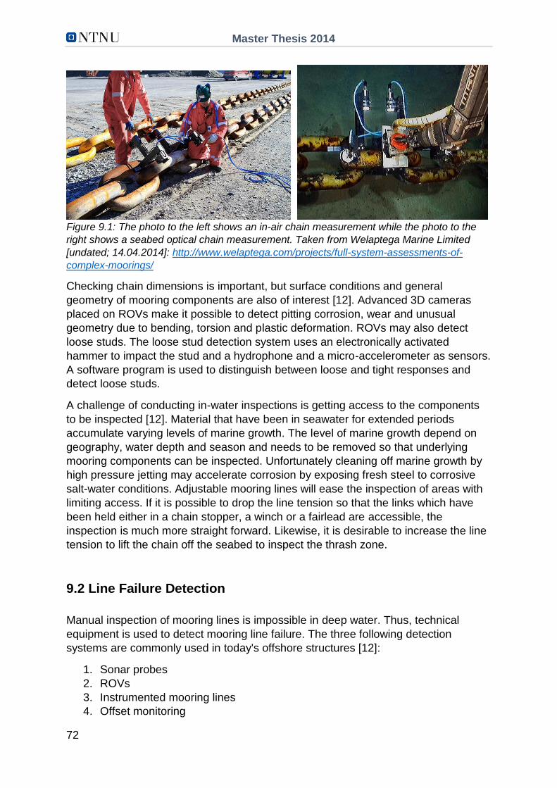
Master Thesis 2014

72

Figure 9.1: The photo to the left shows an in-air chain measurement while the photo to the

right shows a seabed optical chain measurement. Taken from Welaptega Marine Limited

[undated; 14.04.2014]: http://www.welaptega.com/projects/full-system-assessments-of-

complex-moorings/

Checking chain dimensions is important, but surface conditions and general

geometry of mooring components are also of interest [12]. Advanced 3D cameras

placed on ROVs make it possible to detect pitting corrosion, wear and unusual

geometry due to bending, torsion and plastic deformation. ROVs may also detect

loose studs. The loose stud detection system uses an electronically activated

hammer to impact the stud and a hydrophone and a micro-accelerometer as sensors.

A software program is used to distinguish between loose and tight responses and

detect loose studs.

A challenge of conducting in-water inspections is getting access to the components

to be inspected [12]. Material that have been in seawater for extended periods

accumulate varying levels of marine growth. The level of marine growth depend on

geography, water depth and season and needs to be removed so that underlying

mooring components can be inspected. Unfortunately cleaning off marine growth by

high pressure jetting may accelerate corrosion by exposing fresh steel to corrosive

salt-water conditions. Adjustable mooring lines will ease the inspection of areas with

limiting access. If it is possible to drop the line tension so that the links which have

been held either in a chain stopper, a winch or a fairlead are accessible, the

inspection is much more straight forward. Likewise, it is desirable to increase the line

tension to lift the chain off the seabed to inspect the thrash zone.

9.2 Line Failure Detection

Manual inspection of mooring lines is impossible in deep water. Thus, technical

equipment is used to detect mooring line failure. The three following detection

systems are commonly used in today's offshore structures [12]:

1. Sonar probes

2. ROVs

3. Instrumented mooring lines

4. Offset monitoring

http://www.welaptega.com/projects/full-system-assessments-of-complex-moorings/

http://www.welaptega.com/projects/full-system-assessments-of-complex-moorings/

Master Thesis 2014

73

Sonar probes are placed 15-20 meters below a hull [12]. The sonar head is deployed

every 2 weeks in calm weather or after a storm to confirm that all the mooring lines

are intact. A sonar display screen shows the position of the mooring lines seen from

the hull and downwards. The sonar probe system is fairly simple and easy to repair if

something goes wrong with it. However, the system has two important limitations.

Firstly, if a line breaks in the mud, it will still have some line tension and monitored

changes in position may not be sufficient to indicate that a line has failed. Secondly,

a line failure may be undetected for weeks while a severe storm could develop.

Small remotely operated vehicles, known as ROVs, can be deployed directly from the

deck of the FPS itself [12]. Simple inclinometers in ROVs measure mooring line

slopes with respect to gravity. This way it is possible to find out whether the line

tensions are in balance or too slack. A slack line may indicate line failure.

If the detection system is working properly, the simplest way to detect a mooring line

failure is to include a load cell in the line, ideally close to the fairlead where the line

tensions are high [12]. If a load sensor fail, the operating personnel may think that a

line has failed. If all the line tensions are recorded and a line fails, one should see

tension pulses on the adjacent lines. These pulses should be detected if the

recording interval is frequent enough and the load cells are sufficiently sensitive.

Although instrumented mooring lines are easy to operate and provide accurate data,

signal transmission cables are fragile. The equipment may not endure the installation

operation or the harsh environmental loads that may occur during the service life of a

long-term mooring system.

Unit offset monitoring detects offsets due to the unit's equilibrium position [12]. If a

line fails, the equilibrium position change. In theory, this is detected by offset

monitoring. However, if a line fails in moderate weather conditions, it is difficult to

distinguish the change in offset from the normal offset changes due to wind, wave

and current effects. Actually, mooring lines do fail quite often in moderate conditions.

The direction from which the weather comes from may influence the effectiveness of

offset monitoring. For example if a line fails and the weather pushes the unit in the

direction of the failed line, the offset from the equilibrium position will be small

compared to the weather pushing the unit in the opposite direction to the failed line in

which one less line is loaded. As explained, line failures aren't always easy to detect.

In addition, false failure alarms may occur. Few available satellites (poor GPS) or

gyro malfunction may indicate large offsets and cause false failure alarms.

9.3 Extended Service Life

Most engineering components and structures interact with corrosive environments

such as air, humidity, water and salt water [20]. Complete protection against

corrosion is difficult to achieve for long-term mooring systems, thus chains are

normally provided with a corrosion allowance, see table 7.1. Various coatings can

also increase the corrosion resistance. Zinc coating methods such as galvanizing

provide better corrosion resistance. Chromium or nickel electrolytic plating of steel

can increase the corrosion resistance, but also produce undesirable tensile residual

Master Thesis 2014

74

stresses, hairline surface cracks and possibly hydrogen embrittlement. Non-metallic

coatings such as paint, oil, polymers and ceramics can protect against corrosive

environments if they remain continuous. Broken or disrupted coatings can eliminate

their beneficial effects.

Cathodic protection is another widely used method to reduce corrosion damage [36].

The corrosion of a metal surface is controlled by making the surface the cathode of

an electrochemical cell. A sacrificial anode is attached to the metal that needs

protection. The metal surface is polarized until the surface has a uniform potential

and the corrosion reaction is halted. The polarization is caused by the current flow

from the anode to the cathode, driven by the difference in electrochemical potential

between the two materials. The anode is made of highly corrosive metal that needs

to be replaced from time to time. Figure 9.2 shows a typical sacrificial anode used in

mooring systems. For deep-water moorings and large structures, cathodic protection

cannot deliver enough current to provide complete corrosion protection. In such

cases, anodes are connected to a power source to make an impressed current

cathodic protection system.

Figure 9.2: A sacrificial anode is disconnected from the cathodic protection system and

brought onshore to control the rate of corrosion [12, p. 150]

Although coatings and cathodic protection is meant to protect against damage, there

are some accompanying detrimental mechanisms to be aware of. Staining the metal

or acidic treat the metal before galvanizing it may lead to hydrogen embrittlement. In

addition, cathodic protection will cause formation of hydrogen at the metal surface

[37]. The hydrogen atoms can either combine forming hydrogen molecules or

become absorbed in the metal. In the latter case, hydrogen atoms may interact with

the microstructure of the metal subjected to high stresses causing initiation and

growth of hydrogen-related cracks. This mechanism is called hydrogen-induced

stress cracking. According to NS 9415 [38, Appendix I] carbon steel with cathodic

protection must have a yield stress less than 550 MPa and a maximum hardness of

350 HV to prevent hydrogen-induced stress cracking. Additionally the steel must be

designed with a corrosion allowance.

Use of coatings in combination with cathodic protection may lead to disbonding of

non-metallic coatings by chemical mechanisms at the interface between the metal

Master Thesis 2014

75

and the coating [37]. Some coatings, especially those based on epoxy or

polyurethane, have shown good resistance to cathodic disbonding.

Non-metallic coatings will, unlike metallic coatings, drastically reduce the current

demand in a cathodic protected system and hence, the required anode weight [37].

For weight-sensitive structures with long design life, the combination of coating and

cathodic protection is likely to give the most cost-effective corrosion control.

Current drain to components that are electrically connected to the cathodic protected

object must be considered during the design [37]. This may include components that

are regarded as fully resistant to corrosion in seawater and components that do not

need corrosion protection due to high wall thickness relative to expected corrosion

rates. Mooring chains experience current drain at the lower end, at the connection

with the anchor. The current drain shall be accounted for by 30 meters of chain. For

systems with mooring point below the water level, the seawater-exposed section

above this point shall also be included.

Master Thesis 2014

76

CHAPTER 10

Static Analysis

10.1 Analytical Calculations

A two-dimensional model of a chain link has two axis of symmetry. Thus, one fourth of the chain link is sufficient to make a calculation model. The analytical calculation models in this chapter represent half chain links. The models are two-hinged, partly circular frames. A tensile load loads the frames at midpoint. In real life, the external load is not a point load, but a distributed load from an adjacent link over a contact area smaller than the cross-sectional diameter of the link. It is also not quite correct to split the chain link into curved and straight components as shown in Figure 10.1. The so-called straight parts of the chain links have, in fact, a slight curvature. Common chain link dimensions for stud links and studless links have a maximum width larger than the outer diameter of the bended section. The dimensions of the calculation models in Figure 10.1 are based on common link design as described in Chapter 2.2.

a) Model of stud link b) Model of studless link Figure 10.1: Static model of a chain link with external point load F, radius of curvature r and height 2.50 D. D is the nominal cross-sectional diameter. The radius of curvature, r, is equal to 1.15 D for stud links and 1.10 D for studless links. All dimensions are measured from the centerline of the cross section.

If the number of reaction forces exceeds the number of independent equations of equilibrium, the system is statically indeterminate. The static model in Figure 10.1a has one statically indeterminate reaction force. The redundant is found by using the unit load method and the principle of superposition.

The reaction forces at the pinned bearings in Figure 10.1a are calculated as shown in Appendix A and equal to:

Fy = -0.50 F Fx = 0.10 F

Master Thesis 2014

77

Since the calculation model in Figure 10.1b is statically determinate, the reaction forces are easy to calculate and equal to:

Fy = -0.50 F Fx = 0.00 F

The maximum moment is located under the point load with tensile stresses at the outer side of the crown. The shear force and the axial force under the point load are equal to the respective reaction forces.

The load reactions at midpoint of the model in Figure 10.1a are:

M = -0.325 FD V = Fy = -0.50 F N = Fx = 0.10 F

The load reactions at midpoint of the model in Figure 10.1b are:

M = -0.550 FD V = Fy = -0.50 F N = Fx = 0.00 F

10.2 Calculations in Focus Konstruksjon 2014

Focus Konstruksjon 2014 is a beam element program designed to help the user doing static calculations. The computer program provides static results in terms of bending moments, shear forces, axial forces, displacements and buckling modes. Focus uses Eurocodes to calculate the capacity of the structure in the ultimate limit state.

Input data used in static calculations:

- Model: two-dimensional beam segments - Loading: live load, point load with partial safety factor 1.00, no dead load - Finite element length: 5 mm - Type of analysis: linear - Cross section: customized massive circular cross section with diameter equal

to 100 mm - Material properties: customized steel grade corresponding to steel grade R3,

yield stress fy = 410 MPa, elastic modulus E = 210000 MPa, shear modulus G = 81000 MPa and Poisson's ratio μ = 0.3

The results obtained with Focus, in terms of moments, shear forces and axial forces, are listed in Table 10.1.

Master Thesis 2014

78

Table 10.1: M-/V-and N-values for different calculation models in Focus Konstruksjon 2014. The models are loaded with a design point load equal to F. The cross-sectional diameter is equal to D. The radius of curvature, r, is equal to 1.15 D for stud links and 1.10 D for studless links.

Calculation model

Half a chain link without stud

Half a chain link with stud

Whole chain link without stud

Whole chain link with stud

Load [kN] F F F F

Max values:

Moment [kNm] 0.328 FD 0.319 FD 0.439 FD 0.323 FD

Shear load [kN] 0.506 F 0.506 F 0.500 F 0.508 F

Axial load [kN] 0.520 F 0.525 F 0.500 F 0.531 F

Values at midpoint:

Moment [kNm] 0.328 FD 0.319 FD 0.437 FD 0.300 FD

Shear load [kN] 0.489 F 0.506 F 0.500 F 0.489 F

Axial load [kN] 0.099 F 0.140 F 0.011 F 0.142 F

The model consisting of half a chain link without stud in Table 10.1 gets approximately equal results as the models with stud. The models with stud will get an increased axial load at midpoint due to the axial stiffness of the stud.

By modeling the whole chain link without stud, the moment at midpoint increases at the same time as the axial load decreases. Chain links without stud have, as a result of increased moments, the lowest capacity. Moment-/shear force- and axial force diagrams for stud links and studless links are shown in Figure 10.2.

Master Thesis 2014

79

Figure 10.2 a) Moment diagram

Figure 10.2 b) Shear force diagram

Figure 10.2 c) Axial force diagram Figure 10.2: M-/V-and N-diagrams with max values are shown for stud link to the left and studless link to the right. The results are obtained with a two-dimensional linear analysis in the computer program Focus Konstruksjon 2014. The links are loaded with a tensile load of 1000 kN acting at the midpoint of the frame. The cross-sectional diameter is 100 mm.

Master Thesis 2014

80

Figure 10.3 illustrates deformed chain links. The studless link will extend more than the stud link. The deformed links are longer and narrower than the original link design.

Figure 10.3: Deformation of chain links, stud link to the left and studless link to the right. The results are obtained with a two-dimensional linear analysis in the computer program Focus Konstruksjon 2014. The links are loaded with a tensile load equal to 1000 kN acting at the midpoint of the frame. The cross-sectional diameter is 100 mm. The horizontal displacement at the stud is very small for the stud link, but 0.30 mm for the studless link. The vertical displacement under the point load is 0.44 mm for the stud link and 0.60 mm for the studless link.

Table 10.2 shows how external load distributions affect moments, shear forces and axial forces. The source of error using a point load instead of a distributed load is estimated by modeling evenly distributed loads. The actual load on a chain link is a parabolic distributed load over a contact area whose size depends on the external load intensity.

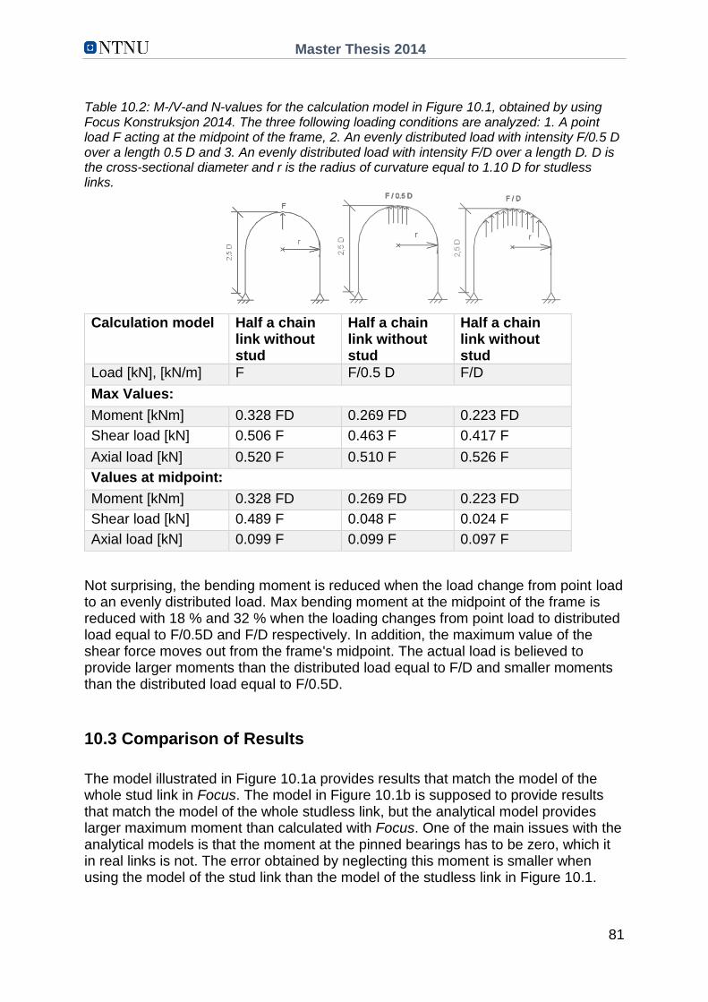
Master Thesis 2014

81

Table 10.2: M-/V-and N-values for the calculation model in Figure 10.1, obtained by using Focus Konstruksjon 2014. The three following loading conditions are analyzed: 1. A point load F acting at the midpoint of the frame, 2. An evenly distributed load with intensity F/0.5 D over a length 0.5 D and 3. An evenly distributed load with intensity F/D over a length D. D is the cross-sectional diameter and r is the radius of curvature equal to 1.10 D for studless links.

Calculation model Half a chain link without stud



Load [kN], [kN/m] F F/0.5 D F/D

Max Values:

Moment [kNm] 0.328 FD 0.269 FD 0.223 FD

Shear load [kN] 0.506 F 0.463 F 0.417 F

Axial load [kN] 0.520 F 0.510 F 0.526 F

Values at midpoint:

Moment [kNm] 0.328 FD 0.269 FD 0.223 FD

Shear load [kN] 0.489 F 0.048 F 0.024 F

Axial load [kN] 0.099 F 0.099 F 0.097 F

Not surprising, the bending moment is reduced when the load change from point load to an evenly distributed load. Max bending moment at the midpoint of the frame is reduced with 18 % and 32 % when the loading changes from point load to distributed load equal to F/0.5D and F/D respectively. In addition, the maximum value of the shear force moves out from the frame's midpoint. The actual load is believed to provide larger moments than the distributed load equal to F/D and smaller moments than the distributed load equal to F/0.5D.

10.3 Comparison of Results

The model illustrated in Figure 10.1a provides results that match the model of the whole stud link in Focus. The model in Figure 10.1b is supposed to provide results that match the model of the whole studless link, but the analytical model provides larger maximum moment than calculated with Focus. One of the main issues with the analytical models is that the moment at the pinned bearings has to be zero, which it in real links is not. The error obtained by neglecting this moment is smaller when using the model of the stud link than the model of the studless link in Figure 10.1.

Master Thesis 2014

82

The stresses at the crown are calculated in Appendix B. These stresses are used to

find a stress concentration factor for stud links.

The geometric stress concentration factor at the inner side of the crown equals:

SCF = σmax/σnom = ( 2.96 F/D2)/(F/2π(D2/4)) = -4.65,

and the geometric stress concentration factor at the outer side of the crown equals:

SCF = σmax/σnom = (1.66 F/D2)/(F/2π(D2/4)) = 2.61.

The vertical displacement under the point load is calculated by using the unit load method, see Appendix A. The calculated vertical displacement due to bending deformation, shear deformation and axial deformation in stud links is 9.896 F/DE. This result corresponds to the displacement calculated with Focus.

The capacities found by using von Mises yield criterion and interaction formulas are

much lower than the proof load and minimum breaking load specified by

manufacturer. For instance, the elastic and plastic capacities of a stud link with cross-

sectional diameter 100 mm and yield stress 410 MPa (for steel grade R3) are

calculated to 1320 kN and 3150 kN respectively (see Appendix B and C). By

comparison, the proof load is 5616 kN while the minimum breaking load is 8028 kN

for a stud link with cross-sectional diameter 100 mm and yield stress 410 MPa. This

shows that capacities cannot be found with capacity formulas based on classic beam

theory or curved beam theory. One reason for this is that the steel may yield during

proof loading. The steel is free to yield because the plastic deformations are local and

restricted to a small area, doing no harm.

The breaking load of chain links is found experimentally and with empirical formulas.

Master Thesis 2014

83

CHAPTER 11

Numerical Analysis

In order to conduct finite element analyses, the software Abaqus 6.12 is used.

Abaqus is a finite element program used for solving structural problems such as

dynamic vibration problems, thermal connections and non-linear statics.

All chains are tested with a mandatory proof test by the manufacturer. The very large

proof load, approximately three times the operational load, is applied to chains and

then removed [2]. The proof load leaves a residual stress field that is present when

chain links enter in operation. As fatigue cracks are normally initiated by a tensile

stress field, the presence of tensile residual stresses may be damaging. When tensile

stresses occur during operation, they are added to the already existing residual

stresses. The resulting tensile stress level may be much higher than predicted during

the design process. On the other hand, a compressive residual stress may be

beneficial if it is subtracted from a tensile one generated during operation.

Finite element analyses was carried out for chains loaded with proof load and a

maximum operational load equal to one fourth of minimum breaking load. The

purpose with these analyses was to study residual stresses in whole chain links and

stress distributions in worn chain links subjected to operational loading. Residual

stresses due to weld geometry and thermal expansion during welding were

considered small close to the flash butt weld. Only residual stresses due to proof

loading were considered in these analyses. Both studless links and stud links were

analyzed.

11.1 Input Data

11.1.1 Geometry

The geometry of the modelled chain links are meant to match the dimensions

provided by ISO 1704 [10] and IACS W22 [11], and described in Chapter 2.2. The

cross-sectional diameter was set to 76 mm.

A three-dimensional model of a chain link has three planes of symmetry, thus one

eight of the link is sufficient to make a calculation model.

Chain links in Abaqus were modelled as one eight of a whole link to save

computational time. The parts were modelled as 3D deformable solids based on a

path sketch and a section sketch as illustrated in Figure 11.1.

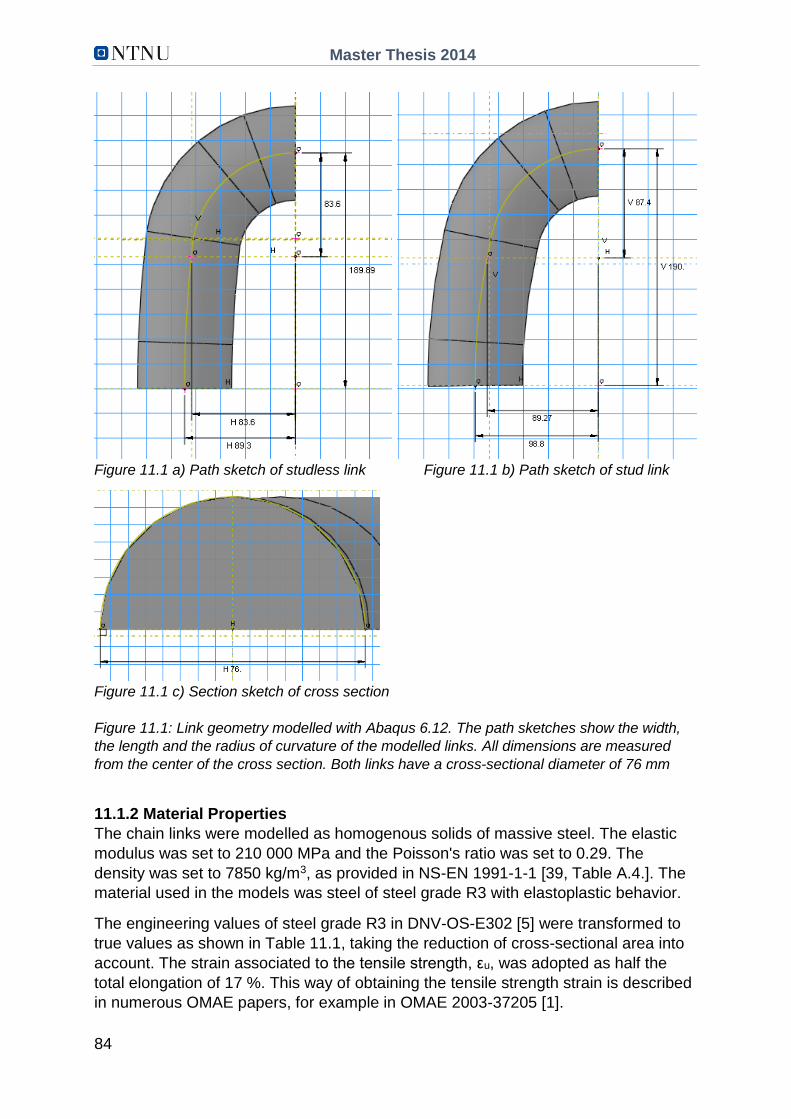
Master Thesis 2014

84

Figure 11.1 a) Path sketch of studless link Figure 11.1 b) Path sketch of stud link

Figure 11.1 c) Section sketch of cross section

Figure 11.1: Link geometry modelled with Abaqus 6.12. The path sketches show the width,

the length and the radius of curvature of the modelled links. All dimensions are measured

from the center of the cross section. Both links have a cross-sectional diameter of 76 mm

11.1.2 Material Properties

The chain links were modelled as homogenous solids of massive steel. The elastic

modulus was set to 210 000 MPa and the Poisson's ratio was set to 0.29. The

density was set to 7850 kg/m3, as provided in NS-EN 1991-1-1 [39, Table A.4.]. The

material used in the models was steel of steel grade R3 with elastoplastic behavior.

The engineering values of steel grade R3 in DNV-OS-E302 [5] were transformed to

true values as shown in Table 11.1, taking the reduction of cross-sectional area into

account. The strain associated to the tensile strength, εu, was adopted as half the

total elongation of 17 %. This way of obtaining the tensile strength strain is described

in numerous OMAE papers, for example in OMAE 2003-37205 [1].

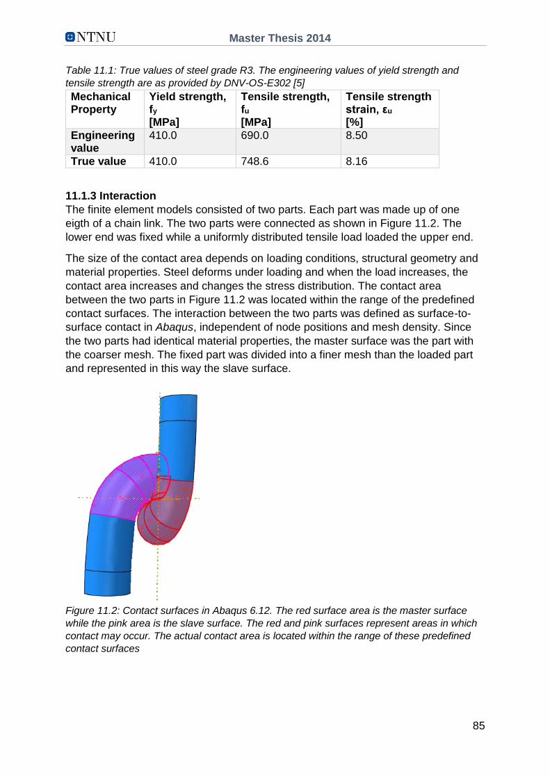
Master Thesis 2014

85

Table 11.1: True values of steel grade R3. The engineering values of yield strength and

tensile strength are as provided by DNV-OS-E302 [5]

Mechanical Property

Yield strength, fy [MPa]

Tensile strength, fu [MPa]

Tensile strength strain, εu [%]

Engineering value

410.0 690.0 8.50

True value 410.0 748.6 8.16

11.1.3 Interaction

The finite element models consisted of two parts. Each part was made up of one

eigth of a chain link. The two parts were connected as shown in Figure 11.2. The

lower end was fixed while a uniformly distributed tensile load loaded the upper end.

The size of the contact area depends on loading conditions, structural geometry and

material properties. Steel deforms under loading and when the load increases, the

contact area increases and changes the stress distribution. The contact area

between the two parts in Figure 11.2 was located within the range of the predefined

contact surfaces. The interaction between the two parts was defined as surface-to-

surface contact in Abaqus, independent of node positions and mesh density. Since

the two parts had identical material properties, the master surface was the part with

the coarser mesh. The fixed part was divided into a finer mesh than the loaded part

and represented in this way the slave surface.

Figure 11.2: Contact surfaces in Abaqus 6.12. The red surface area is the master surface

while the pink area is the slave surface. The red and pink surfaces represent areas in which

contact may occur. The actual contact area is located within the range of these predefined

contact surfaces

Master Thesis 2014

86

Interaction properties defines how surfaces responds to contact. The interaction

properties between the links in Figure 11.2 were defined as tangential contact and

normal contact. The friction coefficient of steel-to-steel contact depends on lubrication

and surface finish and ranges from 0.15 to 0.8. Both of the friction coefficient limits

were included in analyses as the only variable. The two analyses gave practically the

same results, confirming that the friction coefficient had little influence on the finite

element analyses. The friction coefficient was set to 0.7 and the contact was defined

as hard.

11.1.4 Loading and Boundary Conditions

The load was defined as a uniformly distributed surface traction acting perpendicular

to the top surface as shown in Figure 11.3. The proof load and minimum breaking

load on a chain with cross-sectional diameter of 76 mm and steel grade R3 was set

to 3416.8 kN and 4884.3 kN respectively and in accordance with DNV-OS-E302 [5].

The requirements for minimum proof load and minimum breaking load are the same

for stud links and studless links with steel grade R3. The proof load resulted in a

surface traction of 377 MPa, and the load equal to 25 % of the minimum breaking

load resulted in a surface traction of 135 MPa.

In order to prevent rotation of the loaded top surface, the top surface was restrained

against displacement in the x- and z-direction in Figure 11.3. By doing this, the whole

loaded part was restrained against displacement in the z-direction. This may have

reduced the contact area between the two parts. However, the error obtained by

doing this was considered small.

Both of the parts in the finite element models had three planes of symmetry. Each

plane of symmetry, except the load surface, was assigned symmetric boundary

conditions. The symmetric boundary conditions restrained displacement in one

direction and prevented rotation about the two other directions. For example, the

fixed bottom surface was restrained against displacement in y-direction and against

rotation about the x- and z-axis. Figure 11.3 highlights the six boundary surfaces in

red.

Master Thesis 2014

87

Figure 11.3: Loading and boundary conditions in Abaqus 6.12. The model to the right

highlights the surfaces which are assigned boundary conditions. x, y and z are the principal

axes in Abaqus 6.12. The lower end is fixed and will not displace in y-direction while the

upper end is loaded with a uniformly distributed tensile load and free to displace in y-

direction.

11.1.5 Element Type

The finite element models was made of tetrahedrals or hexahedrals. The triangular

prism in Figure 11.4, the so-called wedge element, was not used. The wedge

element is a special or alternative form of solid element and not widely used.

All the solid elements had mid-edge nodes in addition to corner nodes. Such

elements are quadratic. Quadratic elements provide more accurate results than linear

elements, but increase the computational time as well. A quadratic tetrahedral has six

more nodes than a linear tetrahedral and a quadratic hexahedral has twelve more

nodes than a linear one. Each node has three degrees of freedom in terms of nodal

displacements.

The hexahedrals were assigned reduced integration to reduce the computational

time. Reduced integration may also soften the behavior of the elements and improve

the accuracy of the computed results.

Abaqus denotes elements based on element properties. The hexahedrals and

tetrahedrals used in analyses were denoted C3D20R and C3D10 respectively. C3D

stands for a three-dimensional continuum, 20R stands for a 20-node quadratic

hexahedral with reduced integration and 10 stands for a 10-node quadratic

tetrahedral. The hexahedral has 20 nodes and a total of 60 degrees of freedom while

the tetrahedron has 10 nodes and 30 degrees of freedom.

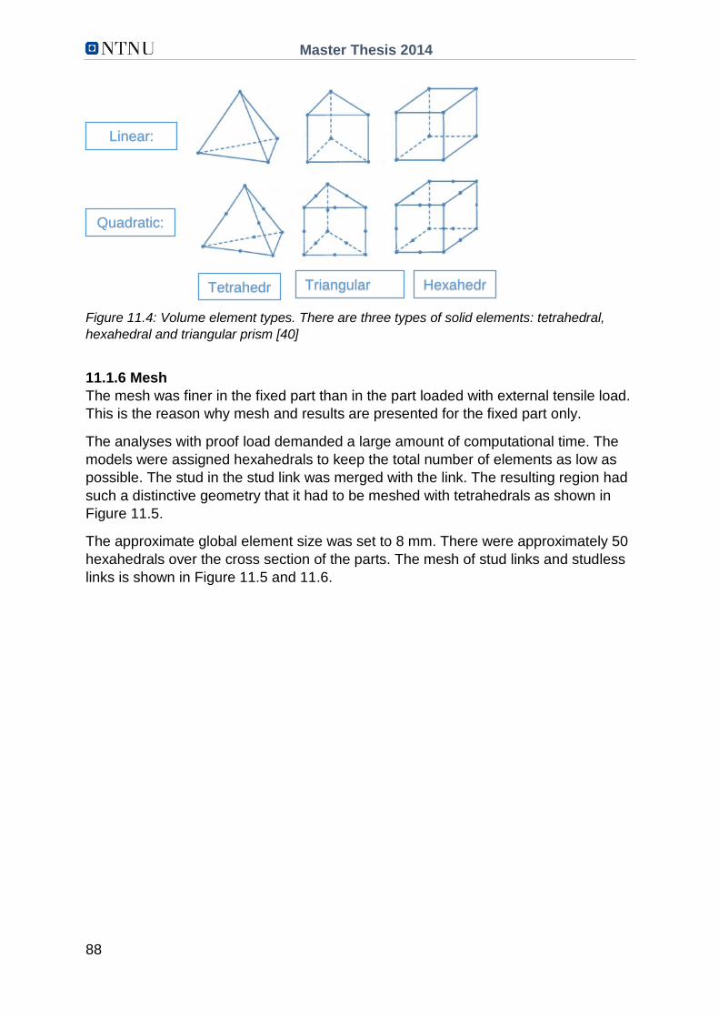
Master Thesis 2014

88

Figure 11.4: Volume element types. There are three types of solid elements: tetrahedral,

hexahedral and triangular prism [40]

11.1.6 Mesh

The mesh was finer in the fixed part than in the part loaded with external tensile load.

This is the reason why mesh and results are presented for the fixed part only.

The analyses with proof load demanded a large amount of computational time. The

models were assigned hexahedrals to keep the total number of elements as low as

possible. The stud in the stud link was merged with the link. The resulting region had

such a distinctive geometry that it had to be meshed with tetrahedrals as shown in

Figure 11.5.

The approximate global element size was set to 8 mm. There were approximately 50

hexahedrals over the cross section of the parts. The mesh of stud links and studless

links is shown in Figure 11.5 and 11.6.

Linear:

Quadratic:

Tetrahedr

Triangular

prism

Hexahedr

al

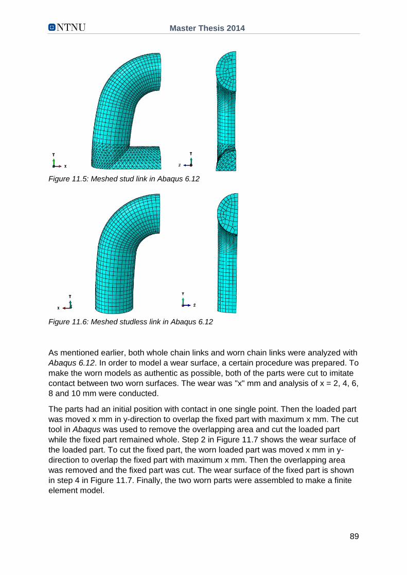
Master Thesis 2014

89

Figure 11.5: Meshed stud link in Abaqus 6.12

Figure 11.6: Meshed studless link in Abaqus 6.12

As mentioned earlier, both whole chain links and worn chain links were analyzed with

Abaqus 6.12. In order to model a wear surface, a certain procedure was prepared. To

make the worn models as authentic as possible, both of the parts were cut to imitate

contact between two worn surfaces. The wear was "x" mm and analysis of x = 2, 4, 6,

8 and 10 mm were conducted.

The parts had an initial position with contact in one single point. Then the loaded part

was moved x mm in y-direction to overlap the fixed part with maximum x mm. The cut

tool in Abaqus was used to remove the overlapping area and cut the loaded part

while the fixed part remained whole. Step 2 in Figure 11.7 shows the wear surface of

the loaded part. To cut the fixed part, the worn loaded part was moved x mm in y-

direction to overlap the fixed part with maximum x mm. Then the overlapping area

was removed and the fixed part was cut. The wear surface of the fixed part is shown

in step 4 in Figure 11.7. Finally, the two worn parts were assembled to make a finite

element model.

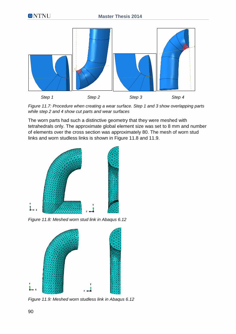
Master Thesis 2014

90

Figure 11.7: Procedure when creating a wear surface. Step 1 and 3 show overlapping parts

while step 2 and 4 show cut parts and wear surfaces

The worn parts had such a distinctive geometry that they were meshed with

tetrahedrals only. The approximate global element size was set to 8 mm and number

of elements over the cross section was approximately 80. The mesh of worn stud

links and worn studless links is shown in Figure 11.8 and 11.9.

Figure 11.8: Meshed worn stud link in Abaqus 6.12

Figure 11.9: Meshed worn studless link in Abaqus 6.12

Step 1 Step 2 Step 3 Step 4

Master Thesis 2014

91

11.2 Results

The models that were analyzed with Abaqus had different loading and geometry. The

proof load was applied only to whole chain links while the maximum operational load

was applied to both whole and worn chain links. Table 11.2 provides an overview

over loading and geometry of different models. Analyses of both stud links and

studless links were conducted for each of the seven models in Table 11.2, giving a

total of 14 job analyses.

Table 11.2: Loading and geometry of models

Model Loading Geometry

Proof load, = 3416.8 kN

Max. operational load, = 1221.1 kN

Whole chain link

Worn chain link [mm]

2 4 6 8 10

Model 1 X X

Model 2 X X

Model 3 X X

Model 4 X X

Model 5 X X

Model 6 X X

Model 7 X X

The results from the analyses are presented as von Mises stresses and maximum

principal stresses. Von Mises stresses are helpful when using failure criteria to

predict failure in ductile materials. However, von Mises yield criterion do not

distinguish between tensile stresses and compressive stresses. When it comes to

fatigue, the sign of the stress is essential. As a rule of thumb, a tensile mean stress

reduces fatigue life while a compressive mean stress increases fatigue life due to a

mean stress equal to zero. The sign of the stress is also a key factor due to crack

initiation. Unlike Mises stresses, the principal stresses are denoted as positive or

negative.

Abaqus automatically average element output at nodes. If the output values at two

elements are within 75 % of each other, they are averaged. This means that if results

from one element differ from the others in more than 25 %, the results will be

averaged at adjacent nodes. The automatic averaging can be turned off in Abaqus.

This is done for all the results presented in this chapter to highlight the very high local

stresses.

Figure 11.10 and 11.11 show the residual stresses in deformed studless links and

stud links. The figures show that the plastic deformations are large, especially in stud

links.

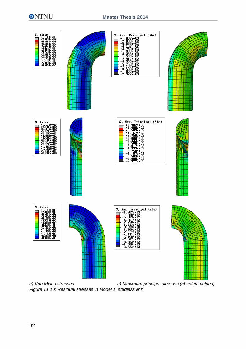
Master Thesis 2014

92

a) Von Mises stresses b) Maximum principal stresses (absolute values)

Figure 11.10: Residual stresses in Model 1, studless link

Master Thesis 2014

93


Figure 11.11: Residual stresses in Model 1, stud link

Master Thesis 2014

94

Figure 11.12 and 11.13 show the stresses due to maximum operational loading in

deformed studless links and stud links.


Figure 11.12: Stresses due to operational loading in Model 2, studless link

Master Thesis 2014

95


Figure 11.13: Stresses due to operational loading in Model 2, stud link

Master Thesis 2014

96

Figure 11.14 and 11.15 show the maximum principal stress field due to maximum

operational loading in deformed studless links. Figure 11.14 shows the stress

distribution in a whole studless link, while Figure 11.15 shows the stress distribution

in worn links. Note that the stresses in the most stressed region are higher in the

whole link than in the worn links. The stress chart in Figure 11.14 and 11.15 is the

same with the same absolute values in order to make the comparison of results

easier.

Figure 11.14: Maximum principal stresses (absolute values) due to operational loading in a

whole studless link, Model 2

Figure 11.15 a) Stress chart, studless link

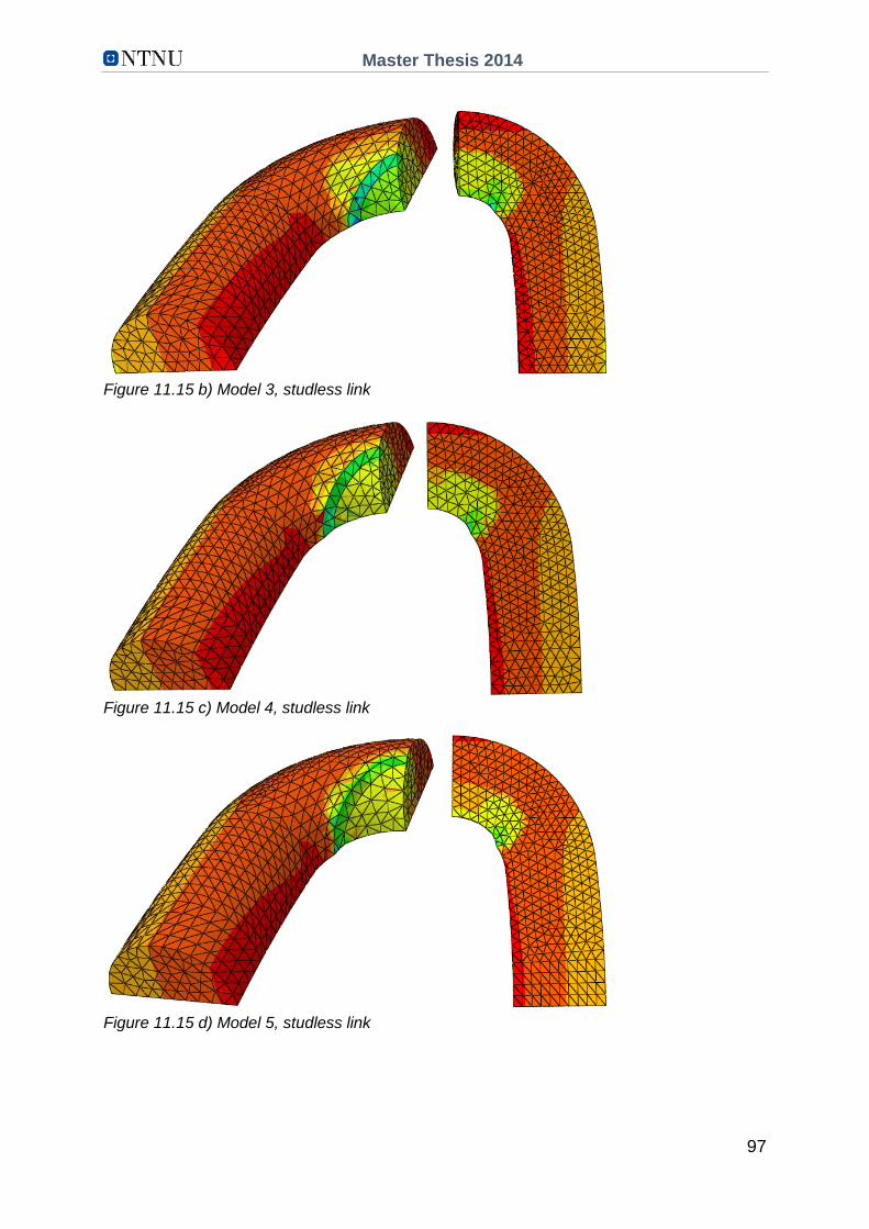
Master Thesis 2014

97

Figure 11.15 b) Model 3, studless link

Figure 11.15 c) Model 4, studless link

Figure 11.15 d) Model 5, studless link

Master Thesis 2014

98

Figure 11.15 e) Model 6, studless link

Figure 11.15 f) Model 7, studless link

Figure 11.15: Maximum principal stresses (absolute values) due to operational loading in

worn studless links

Figure 11.16 and 11.17 show the maximum principal stress field due to operational

loading in deformed stud links. Figure 11.16 shows the stress distribution in a whole

studless link, while Figure 11.17 shows the stress distribution in worn links. Note that

the stresses in the most stressed region are higher in the whole link than in the worn

links. The stress chart in Figure 11.16 and 11.17 is the same with the same absolute

values in order to make the comparison of results easier.

Master Thesis 2014

99

Figure 11.16: Maximum principal stresses (absolute values) due to operational loading in a

whole stud link, Model 2

Figure 11.17 a) Stress chart, stud link

Master Thesis 2014

100

Figure 11.17 b) Model 3, stud link

Figure 11.17 c) Model 4, stud link

Figure 11.17 d) Model 5, stud link

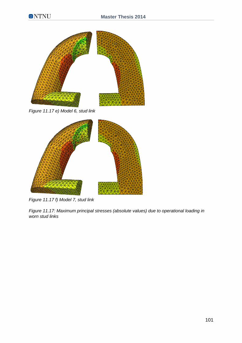
Master Thesis 2014

101

Figure 11.17 e) Model 6, stud link

Figure 11.17 f) Model 7, stud link

Figure 11.17: Maximum principal stresses (absolute values) due to operational loading in

worn stud links

Master Thesis 2014

102

CHAPTER 12

Discussion of Results

12.1 Paths and Stresses

Stress distributions are determined for four different paths in order to provide a

detailed sketch of the stresses in the finite element model. The paths are identified in

Figure 12.1. The four paths are chosen based on assumptions of high stresses in

these areas. The paths are denoted A, B, a and b. The s in Figure 12.1 gives the

direction of the paths. The stresses along the paths are plotted in Figure 12.3 to 12.6

for stud links and studless links.

Figure 12.1: Paths in which stresses are sampled. The "s" shows the direction of the paths.

The paths go along the undeformed shape of the link. Path a and b are longitudinal paths

marked with red lines. They go from the curved part to the straight part of the link. Path a

goes along the inner side while path b goes along the outer side of the link. Path A and B are

transverse paths marked with black lines. They go from a to b in a radial fashion about the

center of the cross section

Path a and b are longitudinal paths along the chain direction while path A and B are

transversal paths. If path A starts at a point with local coordinates (x,y,z) = (0,0,0),

path B starts at (x,y,z) = (-48.864,-42.073,0) for stud links and (x,y,z) = (-44.684,-

36.504,0) for studless links. Path A and B go from a to b in a radial fashion about the

center of the cross section, not through it. Because cracks are more likely to appear

at the surface of a material rather than at internal flaws in the material, stresses along

the surface are plotted to obtain a more detailed understanding of the stress fields in

which cracks may occur.

Only maximum principal stresses with absolute values are plotted. Both residual

stresses and operational stresses are plotted in Figure 12.3 to 12.6. The residual

stresses result from proof loading while the operational stresses result from

maximum operational loading. The proof load is much larger than the operational

load with a magnitude of 70 % of minimum breaking load. Maximum operational load

is set to 25 % of minimum breaking load. Maximum breaking load is equal to 4884.3

kN for steel grade R3 with a cross-sectional diameter equal to 76 mm.

Master Thesis 2014

103

The stresses are typical compressive at the inner side of the bend at the start of path

a. This is not the case for the residual stresses in stud links. The contact area at full

proof loading is quite large with high compressive stresses as shown in Figure 12.2.

When the proof load is offloaded, the stresses are of course reduced, but some

remain. The residual stresses are typical of opposite sign to the initial ones.

Figure 12.2: Stresses at full proof loading in the link to the left and the resulting residual

stresses in the same link to the right.

The very high residual stresses in the stud link towards the end of path a are due to

the sharp edges at the connection between stud and link. These very high stresses

can be ignored, see Chapter 12.5, but a moderate stress raise at this location is

expected.

When it comes to fatigue, the tensile stresses are crucial. The tensile residual

stresses at midpoint of path B are very high like the residual stresses at midpoint of

path A.

The operational stress field in stud links and studless links are quite similar to each

other. The differences in stress fields are due to the introduction of the stud in the

stud link. Plasticity occurs only locally during maximum operational loading and the

deformations are small compared to the deformations during proof loading.

The residual stresses changes from positive to negative all the way along path A.

The highest residual stress appear at approximately 30 % of the path length where

both links have a tensile stress of 400 MPa. The residual stresses along path B have

a maximum value of 250 MPa to 400 MPa in respectively studless links and stud

links. The maximum stress appear at 70 % of the path length. The very high residual

stress in stud links at 80 % of the path length is due to sharp edges near the stud.

The operational stresses along path a and A and along path b and B are almost

identical, or at least of the same shape. The operational compressive stresses are

higher than -1000 MPa at the start of path a and A and change to positive at 10 % to

40 % of the path length. The operational stresses are 300 MPa to 500 MPa at the

start of path b and B and change to negative at 40 % to 75 % of the path length.

Master Thesis 2014

104

Figure 12.3: Residual stress along path a and b in Model 1

Figure 12.4: Residual stress along path A and B in Model 1

Figure 12.5: Maximum operational stress along path a and b in Model 2

-1600-1400-1200-1000

-800-600-400-200

0200400600800

1000

0 0,1 0,2 0,3 0,4 0,5 0,6 0,7 0,8 0,9 1

Max

pri

nci

pal

str

ess,

ab

solu

te v

alu

e [M

Pa]

s, normalized distance [-]

Residual stresses, path a

Stud link Studless link

-600

-500

-400

-300

-200

-100

0

100

200

0 0,1 0,2 0,3 0,4 0,5 0,6 0,7 0,8 0,9 1

Max

pri

nci

pal

str

ess,

ab

solu

te v

alu

e [M

Pa]


Residual stresses, path b


-800-700-600-500-400-300-200-100

0100200300400500600

0 0,1 0,2 0,3 0,4 0,5 0,6 0,7 0,8 0,9 1

Max

pri

nci

pal

str

ess,

ab

solu

te v

alu

e[M

Pa]


Residual stresses, path A


-500

-400

-300

-200

-100

0

100

200

300

400

500

0 0,1 0,2 0,3 0,4 0,5 0,6 0,7 0,8 0,9 1

Max

pri

nci

pal

str

ess,

ab

solu

te v

alu

e

[MP

a]


Residual stresses, path B


-2000-1800-1600-1400-1200-1000

-800-600-400-200

0200400600

0 0,1 0,2 0,3 0,4 0,5 0,6 0,7 0,8 0,9 1

Max

pri

nci

pal

str

ess,

ab

solu

te v

alu

e [M

Pa]


Operational stress, path a


-300

-200

-100

0

100

200

300

400

500

0 0,1 0,2 0,3 0,4 0,5 0,6 0,7 0,8 0,9 1

Max

pri

nci

pal

str

ess,

ab

solu

te v

alu

e [M

Pa]


Operational stress, path b


Master Thesis 2014

105

Figure 12.6: Maximum operational stress along path A and B in Model 2

Worn links are assumed to cause the greatest changes in stress distribution along

path A. Therefore, only path A is considered when plotting stresses in worn links.

Worn links are subjected to proof loading before the wear starts. That is why only

operational stresses are plotted for worn links. Maximum wear takes place at section

A when the chain is exposed to pure tension. Maximum wear is modelled as 2 mm,

4 mm, 6 mm, 8 mm and 10 mm, which corresponds to 2.6 %, 5.3 %, 7.9 %, 10.5 %

and 13.2 % reduction of the cross-sectional diameter.

The contact area between two links increases with increasing wear. When the

contact area increases, the contact pressure decreases. This can be seen in the

figures below. The whole link has in general a higher maximum compressive stress

and a smaller compressive area than the worn links in Figure 12.7 and 12.8.

However, the deformed area of the whole links due to prior proof loading is not

considered, see Chapter 12.5, and the positive effects of wear might be

overestimated.

The maximum compressive stress along path A appears at the sharp edge at the end

of the wear surface. The tensile stresses on the other hand are almost constant

towards the end of path A. The whole link has in general a higher maximum tensile

stress than the worn links although the worn links have a smaller cross-sectional

diameter at section A. It seems like the benefits of a larger contact area surpasses

the disadvantages of a smaller cross-sectional diameter in worn links. This

assumption is of course only valid to a certain extent of wear. At some point the wear

is large enough to cause ductile or brittle failure of the chain link. This will happen

when the maximum reduction of cross-sectional diameter is larger than 13 %, but at

the same time, the extent of wear has to be realistic.

-1600

-1400

-1200

-1000

-800

-600

-400

-200

0

200

400

0 0,1 0,2 0,3 0,4 0,5 0,6 0,7 0,8 0,9 1

Max

pri

nci

pal

str

ess,

ab

solu

te v

alu

e [M

Pa]


Operational stress, path A


-100

0

100

200

300

400

500

0 0,1 0,2 0,3 0,4 0,5 0,6 0,7 0,8 0,9 1

Max

pri

nci

pal

str

ess,

ab

solu

te v

alu

e [M

Pa]


Operational stress, path B


Master Thesis 2014

106

Figure 12.7: Maximum operational stress along path A in Model 2, 3, 4, 5, 6 and 7, stud links

Figure 12.8: Maximum operational stress along path A in Model 2, 3, 4, 5, 6 and 7, studless

links

12.2 Critical Points

High stresses occur at the start and at the end of each of the four paths and at

midpoint of path A and B. A total of eight points are considered as critical. Table 12.1

lists these critical points and their locations.

-1600

-1400

-1200

-1000

-800

-600

-400

-200

0

200

400

600

0 0,1 0,2 0,3 0,4 0,5 0,6 0,7 0,8 0,9 1

Max

pri

nci

pal

str

ess,

ab

solu

te v

alu

e[M

Pa]


Operational stress in stud link, path A

Model 2

Model 3

Model 4

Model 5

Model 6

Model 7

-1400

-1200

-1000

-800

-600

-400

-200

0

200

400

0 0,1 0,2 0,3 0,4 0,5 0,6 0,7 0,8 0,9 1

Max

pri

nci

pal

str

ess,

ab

solu

te v

alu

e[M

Pa]


Operational stress in studless link, path A

Model 2

Model 3

Model 4

Model 5

Model 6

Model 7

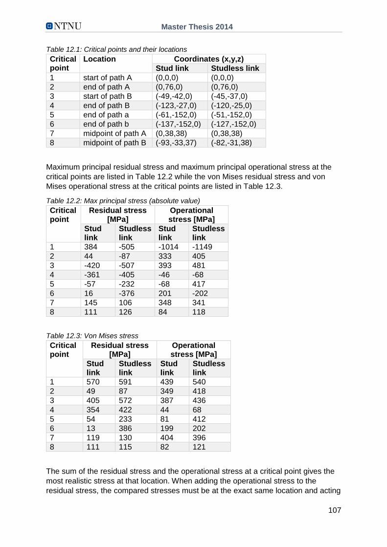
Master Thesis 2014

107

Table 12.1: Critical points and their locations

Critical point

Location Coordinates (x,y,z)


1 start of path A (0,0,0) (0,0,0)

2 end of path A (0,76,0) (0,76,0)

3 start of path B (-49,-42,0) (-45,-37,0)

4 end of path B (-123,-27,0) (-120,-25,0)

5 end of path a (-61,-152,0) (-51,-152,0)

6 end of path b (-137,-152,0) (-127,-152,0)

7 midpoint of path A (0,38,38) (0,38,38)

8 midpoint of path B (-93,-33,37) (-82,-31,38)

Maximum principal residual stress and maximum principal operational stress at the

critical points are listed in Table 12.2 while the von Mises residual stress and von

Mises operational stress at the critical points are listed in Table 12.3.

Table 12.2: Max principal stress (absolute value)

Critical point

Residual stress [MPa]

Operational stress [MPa]

Stud link

Studless link

Stud link

Studless link

1 384 -505 -1014 -1149

2 44 -87 333 405

3 -420 -507 393 481

4 -361 -405 -46 -68

5 -57 -232 -68 417

6 16 -376 201 -202

7 145 106 348 341

8 111 126 84 118

Table 12.3: Von Mises stress

Critical point



Stud link

Studless link

Stud link

Studless link

1 570 591 439 540

2 49 87 349 418

3 405 572 387 436

4 354 422 44 68

5 54 233 81 412

6 13 386 199 202

7 119 130 404 396

8 111 115 82 121

The sum of the residual stress and the operational stress at a critical point gives the

most realistic stress at that location. When adding the operational stress to the

residual stress, the compared stresses must be at the exact same location and acting

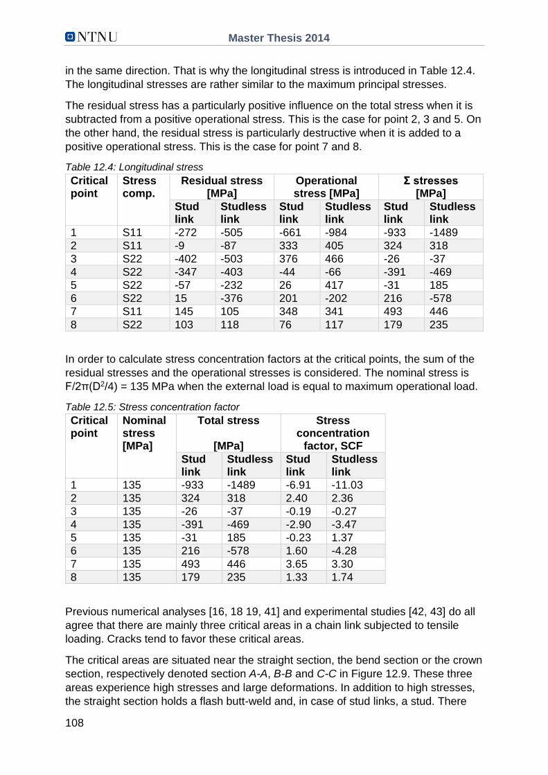
Master Thesis 2014

108

in the same direction. That is why the longitudinal stress is introduced in Table 12.4.

The longitudinal stresses are rather similar to the maximum principal stresses.

The residual stress has a particularly positive influence on the total stress when it is

subtracted from a positive operational stress. This is the case for point 2, 3 and 5. On

the other hand, the residual stress is particularly destructive when it is added to a

positive operational stress. This is the case for point 7 and 8.

Table 12.4: Longitudinal stress

Critical point

Stress comp.



Σ stresses [MPa]

Stud link

Studless link

Stud link

Studless link

Stud link

Studless link

1 S11 -272 -505 -661 -984 -933 -1489

2 S11 -9 -87 333 405 324 318

3 S22 -402 -503 376 466 -26 -37

4 S22 -347 -403 -44 -66 -391 -469

5 S22 -57 -232 26 417 -31 185

6 S22 15 -376 201 -202 216 -578

7 S11 145 105 348 341 493 446

8 S22 103 118 76 117 179 235

In order to calculate stress concentration factors at the critical points, the sum of the

residual stresses and the operational stresses is considered. The nominal stress is

F/2π(D2/4) = 135 MPa when the external load is equal to maximum operational load.

Table 12.5: Stress concentration factor

Critical point

Nominal stress [MPa]

Total stress

[MPa]

Stress concentration

factor, SCF

Stud link

Studless link

Stud link

Studless link

1 135 -933 -1489 -6.91 -11.03

2 135 324 318 2.40 2.36

3 135 -26 -37 -0.19 -0.27

4 135 -391 -469 -2.90 -3.47

5 135 -31 185 -0.23 1.37

6 135 216 -578 1.60 -4.28

7 135 493 446 3.65 3.30

8 135 179 235 1.33 1.74

Previous numerical analyses [16, 18 19, 41] and experimental studies [42, 43] do all

agree that there are mainly three critical areas in a chain link subjected to tensile

loading. Cracks tend to favor these critical areas.

The critical areas are situated near the straight section, the bend section or the crown

section, respectively denoted section A-A, B-B and C-C in Figure 12.9. These three

areas experience high stresses and large deformations. In addition to high stresses,

the straight section holds a flash butt-weld and, in case of stud links, a stud. There

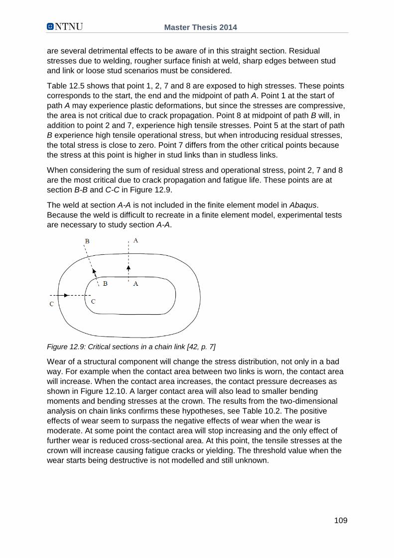
Master Thesis 2014

109

are several detrimental effects to be aware of in this straight section. Residual

stresses due to welding, rougher surface finish at weld, sharp edges between stud

and link or loose stud scenarios must be considered.

Table 12.5 shows that point 1, 2, 7 and 8 are exposed to high stresses. These points

corresponds to the start, the end and the midpoint of path A. Point 1 at the start of

path A may experience plastic deformations, but since the stresses are compressive,

the area is not critical due to crack propagation. Point 8 at midpoint of path B will, in

addition to point 2 and 7, experience high tensile stresses. Point 5 at the start of path

B experience high tensile operational stress, but when introducing residual stresses,

the total stress is close to zero. Point 7 differs from the other critical points because

the stress at this point is higher in stud links than in studless links.

When considering the sum of residual stress and operational stress, point 2, 7 and 8

are the most critical due to crack propagation and fatigue life. These points are at

section B-B and C-C in Figure 12.9.

The weld at section A-A is not included in the finite element model in Abaqus.

Because the weld is difficult to recreate in a finite element model, experimental tests

are necessary to study section A-A.

Figure 12.9: Critical sections in a chain link [42, p. 7]

Wear of a structural component will change the stress distribution, not only in a bad

way. For example when the contact area between two links is worn, the contact area

will increase. When the contact area increases, the contact pressure decreases as

shown in Figure 12.10. A larger contact area will also lead to smaller bending

moments and bending stresses at the crown. The results from the two-dimensional

analysis on chain links confirms these hypotheses, see Table 10.2. The positive

effects of wear seem to surpass the negative effects of wear when the wear is

moderate. At some point the contact area will stop increasing and the only effect of

further wear is reduced cross-sectional area. At this point, the tensile stresses at the

crown will increase causing fatigue cracks or yielding. The threshold value when the

wear starts being destructive is not modelled and still unknown.

Master Thesis 2014

110

Figure 12.10: S22-stresses in stud links. The link to the left is whole while the one to the right

is worn with maximum 10 mm reduction of cross-sectional diameter. Both links are exposed

to maximum operational load. The absolute value of S22 changes from -1419 MPa in the

whole link to -696 MPa in the worn link. The stresses are spread over a larger area in the

worn link.

One of the negative effects of wear is the abrupt change in geometry close to the

edge of the wear surface. The sharper edges the higher stress concentration. Real

wear surfaces may have sharper or smoother edges than modeled with Abaqus.

However, the highest compressive stress in a worn link appear at the edge of the

wear surface. Remember that both tensile load, shear load and torsion may cause

cracks. The three respective crack modes are described in Chapter 3.3. Figure 12.11

shows cracking at the edge of a wear surface.

Figure 12.11: Crack propagation at the edge of a wear surface [41, p. 2]

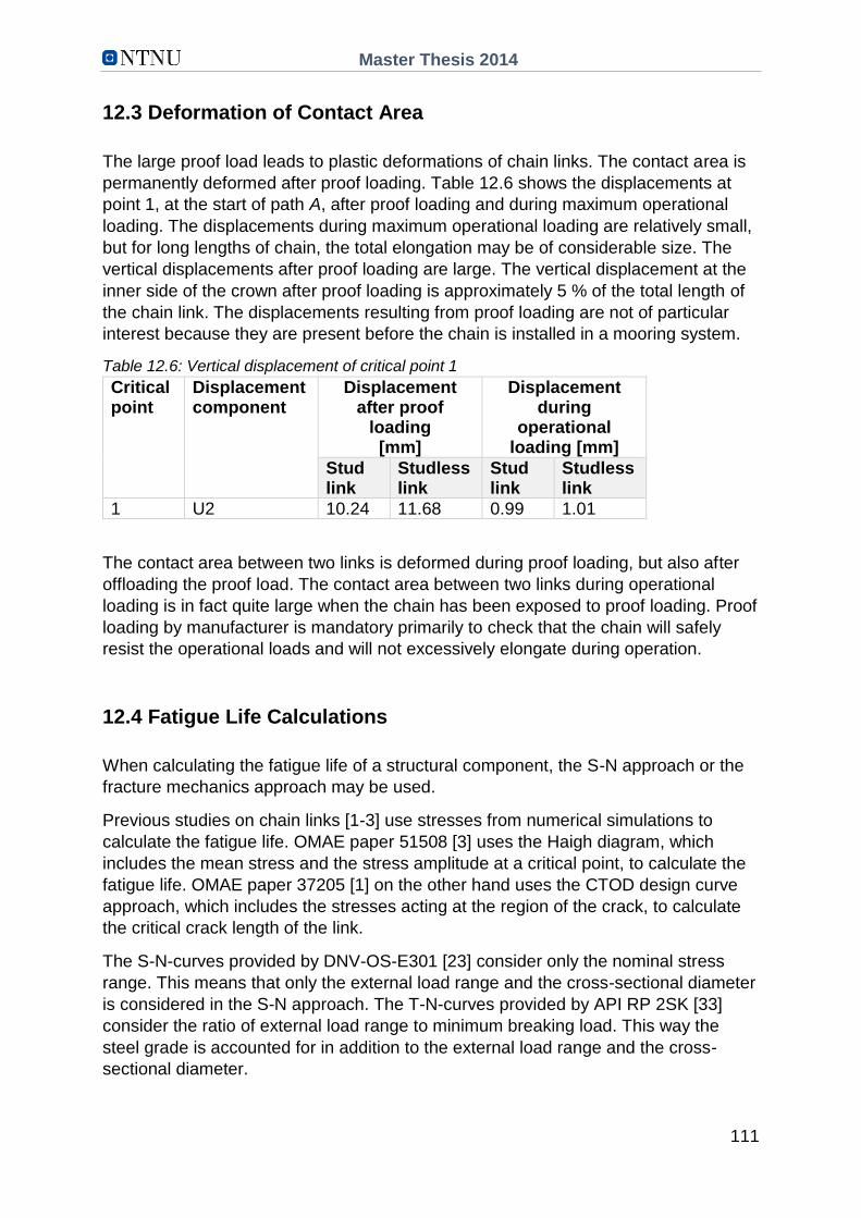
Master Thesis 2014

111

12.3 Deformation of Contact Area

The large proof load leads to plastic deformations of chain links. The contact area is

permanently deformed after proof loading. Table 12.6 shows the displacements at

point 1, at the start of path A, after proof loading and during maximum operational

loading. The displacements during maximum operational loading are relatively small,

but for long lengths of chain, the total elongation may be of considerable size. The

vertical displacements after proof loading are large. The vertical displacement at the

inner side of the crown after proof loading is approximately 5 % of the total length of

the chain link. The displacements resulting from proof loading are not of particular

interest because they are present before the chain is installed in a mooring system.

Table 12.6: Vertical displacement of critical point 1

Critical point

Displacement component

Displacement after proof

loading [mm]

Displacement during

operational loading [mm]

Stud link

Studless link

Stud link

Studless link

1 U2 10.24 11.68 0.99 1.01

The contact area between two links is deformed during proof loading, but also after

offloading the proof load. The contact area between two links during operational

loading is in fact quite large when the chain has been exposed to proof loading. Proof

loading by manufacturer is mandatory primarily to check that the chain will safely

resist the operational loads and will not excessively elongate during operation.

12.4 Fatigue Life Calculations

When calculating the fatigue life of a structural component, the S-N approach or the

fracture mechanics approach may be used.

Previous studies on chain links [1-3] use stresses from numerical simulations to

calculate the fatigue life. OMAE paper 51508 [3] uses the Haigh diagram, which

includes the mean stress and the stress amplitude at a critical point, to calculate the

fatigue life. OMAE paper 37205 [1] on the other hand uses the CTOD design curve

approach, which includes the stresses acting at the region of the crack, to calculate

the critical crack length of the link.

The S-N-curves provided by DNV-OS-E301 [23] consider only the nominal stress

range. This means that only the external load range and the cross-sectional diameter

is considered in the S-N approach. The T-N-curves provided by API RP 2SK [33]

consider the ratio of external load range to minimum breaking load. This way the

steel grade is accounted for in addition to the external load range and the cross-

sectional diameter.

Master Thesis 2014

112

However, S-N-curves for higher steel grades may exceed the curves provided by

DNV. Chain manufacturers may specify higher fatigue strength for their chains than

calculated with DNV's S-N-curves. If so, the higher fatigue strength must be

documented and the new S-N-curves must be approved by DNV.

The S-N-curves provided by DNV and the T-N-curves provided by API do not take

the stress field or the maximum stress in the chain link into account.

12.4.1 Fatigue Life Calculations Using S-N-curves and T-N-curves

Assume that the cyclic load is the same for stud links and studless links with steel

grade R3 and cross-sectional diameter equal to 76 mm. The cyclic load has a

maximum value equal to 25 % of minimum breaking load and minimum value equal

to 10 % of maximum breaking load.

Table 12.7: Predicted fatigue life using the S-N approach or the T-N approach. The predicted

fatigue lives are found by using Figure 8.4, Figure 8.5, Equation 8.2, and Equation 8.3

Calculation method

Parameters Predicted fatigue life, Nt


S-N approach Nominal stress range, ∆σ = 733·103/2π (762/4) = 81 MPa

225 800 112 900

T-N approach Ratio of tension range to minimum breaking load, ∆T/MBL = (0.25 – 0.10) 4884/ 0.223·762 (44 – 0.08·76) = 0.15

296 300 93 600

The predicted fatigue lives are quite similar to each other when using the S-N

approach contra the T-N approach. The studless link has a shorter predicted fatigue

life than the stud link. However, the difference between the predicted fatigue lives of

the two links is larger when using the T-N approach than using the S-N approach.

12.4.2 Fatigue Life Calculations Using Numerical Results

Assume that the cyclic load is the same for stud links and studless links with steel

grade R3 and cross-sectional diameter equal to 76 mm. The cyclic load has a

maximum value equal to 25 % of minimum breaking load and minimum value equal

to 10 % of maximum breaking load.

As a simplification the R-ratio at the critical point with the highest tensile stress is set

to σmin/σmax = 0.1/0.25 = 0.4. The most critical point in the finite element models is

point 7 when considering total stresses (maximum principal residual stress plus

maximum principal operational stress). The mean stress and the stress amplitude at

point 7 is calculated based on maximum stress and R-ratio. The stresses are listed in

Table 12.8.

Master Thesis 2014

113

Table 12.8: Total maximum stress, mean stress and stress amplitude at critical point 7.

Maximum loading is 25 % of MBL and R = 0.4

Critical point

Maximum stress [MPa]

Mean stress [MPa]

Stress amplitude [MPa]

Stud link

Studless link

Stud link

Studless link

Stud link

Studless link

7 493.0 446.0 345.1 312.2 147.9 133.8

OMAE paper 51508 [3] and Mechanical Engineering Design [35] describe how to

incorporate stresses at critical points in fatigue calculations.

In this example, the Goodman line in Figure 8.9 is considered. The parameters that

are used in these fatigue calculations are estimated in accordance with Mechanical

Engineering Design [35].

ka = 0.52 (hot-rolled)

kb = 0.86 (round bar in bending not rotating)

kc = 1 (bending)

kd = 1 (room temperature)

ke = 1

f = 0.900, as in OMAE paper 51508 [3]

Table 12.9: Predicted fatigue life using the Haigh diagram and the Goodman line. The

predicted fatigue life is found by using Equation 8.9

Calculation method

Parameters Predicted fatigue life, Nt


Goodman line Mean stress and stress amplitude from Table 12.8

41 360 107 650

The stud link has a shorter predicted fatigue life than the studless link. This outcome

is actually very surprising. When using stresses from numerical simulations instead of

nominal stresses, the fatigue life of stud links is reduced drastically while the fatigue

life of studless links stays almost the same. This is due to the considered critical

point. Point 7 is one of the few critical points that experience higher stress in stud

links than in studless links.

12.5 Possible Sources of Error

There are some modeling errors to be aware of, i.e. errors due to the transformation

of a physical structure into a mathematical model.

The finite element models of chain links are made as similar to actual chain links as

possible. The width, length and radius of curvature of the links in the finite element

models are identical to the dimension of standardized common chain links. However,

the design of studs is simplified due to lack of information about common stud

designs. The modelled studs have a circular cross section with a constant cross-

sectional diameter equal to the link diameter, while common studs have an elliptical

Master Thesis 2014

114

cross section with varying dimensions in the longitudinal direction of the stud. When

modelling the stud as a circular bar with constant cross section, the stud is

approximately perpendicular to the rest of the link. The sharp edges of almost 90

degrees between the stud and the link result in very high stresses in the surrounding

areas. The stresses obtained from numerical calculations are most likely higher than

actual stresses close to the stud ends.

Type and size of loading in addition to load direction will make the basis for the wear

surface. The modelled wear surface may differ from actual wear surfaces. Actual

wear surfaces may have sharper or smoother edges than the modelled wear

geometry.

The contact area between two links during operational loading is in fact quite large

when the chain has been exposed to proof loading. The proof load leaves a plastic

deformed contact area, but this is not considered in the analyses. However, not

considering such an increased contact area will most likely result in higher

operational stresses than actual contact stresses in whole links. The main issue

occurs when comparing operational stresses in worn links to the very high

operational stresses in whole undeformed links. This may overestimate the positive

effects of wear.

The finite element models consists of two links where one of the links is fixed while

the other one is subjected to a tensile load. The load surface is restrained against

displacement in x- and z-direction in order to prevent rotation of the top surface and

the load. However, Abaqus restrains not only the top surface, but also the rest of the

link against displacement in z-direction. This may reduce the contact area between

the fixed and loaded link. However, the fixed link is able to rotate and results are

presented for this link only.

Master Thesis 2014

115

CHAPTER 13

Comparison of Analytical and Numerical Results

The two analytical calculation models in Figure 10.1 are meant to represent half a

studless link and half a stud link, but only one of them provides satisfactory results.

The calculation model in Figure 10.1b provides too large moments at the crown,

while the model in Figure 10.1a provides moments that are close to the results for

whole stud links in Focus. However, there are some issues with it. The moment and

the horizontal displacement at the pinned bearings have to be zero, which it in real

links are not.

The analytical calculated vertical displacement at the crown is too small compared to

the numerical result. This is because analytical calculations only consider elastic

material behavior. In addition, the analytical calculation model is too stiff and unable

to move horizontally at the bearings.

The analytical calculation model is not fully realistic, but the calculated stress

concentration factor at the crown is close to what is numerically calculated. This may

confirm that the calculation formulas for curved beams provide realistic results and

that the assumed hyperbolic stress distribution in curved beams match the actual

stress distribution in chain links.

Figure 13.1 compare analytical and numerical results for stud links. The analytical

calculations are shown in Appendix A and B. The stress concentration factors at the

crown are calculated as the ratio of longitudinal stress to nominal stress when

external load is maximum operational load equal to 25 % of minimum breaking load.

Table 13.1: Calculated vertical displacement and stress concentration factor at the crown in stud links when subjected to maximum operational loading. The vertical displacements correspond to the vertical displacement at the inner side of the crown of half a stud chain link

Type of calculation

Vertical displacement at the inner side of the crown [mm]

Stress concentration factor at the inner side of the crown

Stress concentration factor at the outer side of the crown

2D Analytical 0.38 -4.65 2.61

3D Numerical 0.99 -4.90 2.47

Master Thesis 2014

116

CHAPTER 14

Conclusion

There are mainly two types of chain links; links with a transverse stud connecting the

link at midpoint and links without a stud. Stud links are heavy and stiff compared to

studless links, but the required minimum breaking load is the same for both types of

chain links. Formulas used to determine the capacity of chains are purely empirical

and based on experience and experimental testing.

As a simplification, chain links are divided into straight and curved parts. The curved

parts are comparable to curved beams while the straight parts are comparable to

straight beams. In straight structural parts, the normal stresses vary linearly over the

cross-section, but if the structural part is curved, the assumptions of stress

distribution become inaccurate. In curved beams, the bending stresses vary in a

hyperbolic fashion over the cross section. However, the stress calculated at the

crown using the curved beam formula match the longitudinal stress obtained by using

numerical calculations.

All mooring chains are proof loaded by manufacturer before they are put into service.

The proof load is approximately 70 % of minimum breaking load. This large proof

load causes plastic deformations and residual stresses in chain links. The residual

stresses may be of significant size, but they are not accounted for in traditional

design of mooring chains. The actual stress in a chain link is the sum of residual

stress and operational stress. When introducing residual stresses, the stress field

changes dramatically for the better, or for the worse. High residual tensile stresses

are particularly damaging when they are added to a tensile operational stress. The

resulting tensile stresses may cause initiation and propagation of cracks.

The finite element models had a cross-sectional diameter equal to 76 mm and steel

grade R3, giving a minimum proof load of 3416.8 kN and a minimum breaking load of

4884.3 kN. Maximum operational load was set to 25 % of minimum breaking load.

Eight points in the finite element models were considered critical due to high

stresses. The critical points were located at the crown, at the bend and at the straight

region in stud links and studless links. All the critical points were located at the link

surface because fatigue cracks tend to appear at the surface of a material.

Longitudinal residual stresses and operational stresses at the critical points were

summed in order to calculate total stresses. The most critical points were at the outer

side of the link at the crown, at the middle of the link surface at the crown and at the

middle of the link surface at the bend. The stress concentration factors at the most

critical points were respectively 2.40, 3.65 and 1.33 for stud links and 2.36, 3.30 and

1.74 for studless links. The highest tensile stress occurred at the crown section of the

stud link.

Wear will primarily reduce the cross-sectional diameter of a chain link. When the

diameter is reduced, the normal stresses and shear stresses increase. In addition,

the wear surface may have some sharp edges causing local stress raise. The highest

Master Thesis 2014

117

compressive stresses in a worn link appear at the edge of the wear surface where

the sharpest edges tend to appear. However, wear at the contact surface between

links has some positive effects too. Wear at the contact area will lead to a larger

contact area and lower contact pressure. A larger contact area will also lead to

smaller bending moments and lower bending stresses at the crown. However, at

some point, the contact area will stop increasing and the only effect of further wear is

reduced cross-sectional area. The positive effects of wear seem to surpass the

negative effects of wear for the analyzed worn links where the reduction of cross-

sectional diameter is 2.6 % to 13.2 %. This assumption is only valid when the wear is

moderate. The threshold value when the wear starts being destructive is not

modelled and therefore more than 13 % reduction of cross-sectional diameter.

The operational load was applied to whole chain links and worn chain links without

plastic deformations. This means that the increased contact area due to prior proof

loading was neglected. Thus, the positive effects of wear may have been

overestimated.

Fatigue is a weakest link process that depends on the local stress in a structural

component. In general, a tensile mean stress reduces fatigue life while a

compressive mean stress increases fatigue life due to a mean stress equal to zero. A

cyclic load with maximum value equal to 25 % of minimum breaking load and

minimum value equal to 10 % of maximum breaking load was used in the fatigue

calculations. When using the S-N-curves provided by DNV, the fatigue life was

calculated to 225 800 cycles to failure for stud links and 112 900 cycles to failure for

studless links. When using the T-N-curves provided by API, the fatigue life was

calculated to 296 300 cycles to failure for stud links and 93 600 cycles to failure for

studless links. The studless link had a shorter predicted fatigue life than the stud link.

However, the difference between the predicted fatigue lives of the two links was

bigger when using the T-N approach than using the S-N approach. When using the

Goodman line and maximum tensile stress obtained by numerical calculations, the

fatigue life was calculated to 41 360 cycles to failure for stud links and 107 650 cycles

to failure for studless links. The predicted fatigue life of stud links was reduced

drastically by using stresses from numerical calculations instead of nominal stresses.

This is because the considered maximum tensile stress was higher in stud links than

in studless links.

Master Thesis 2014

118

CHAPTER 15

Suggestions for Future Studies

This study focus on pure tensile load as the only external loading. Chains in real life

are in some extent exposed to bending and torsion as well. Bending is primarily a

problem when the contact area between two links is deformed or worn. The irregular

contact area creates a locking mode and prevents the links from rolling. Torsion on

the other hand may be a problem if the chain is installed with a twist or if the chain is

connected to mooring components that are not torque balanced.

Analyses of chain links subjected to tension in combination with out-of-plane bending

and chain links subjected to tension in combination with torsion are of interest.

Analysis of both whole links and worn links may give interesting and useful

information.

When it comes to fatigue, further studies on standards, recommended practices and

other regulations are highly recommended. Offshore standards and recommended

practices are generally sparse on details concerning assumptions that form the basis

for fatigue calculations. For example, the S-N-curves provided by Offshore Standard

DNV-OS-E301 [23] say nothing about steel grade. In addition, the standard says

nothing about the stress distribution or critical areas in chain links. The nominal

stress is a parameter in the S-N-curves, but the nominal stress is not representative

for actual stresses in chain links. The hot spot stresses resulting from the complex

geometry of chain links are much higher than the nominal stress. The stress

concentration factor that forms the basis for these curves and the location of this

stress concentration is not known without further investigations.

Master Thesis 2014

119

References

1. Pacheco PMCL, Kenedi PP, Jorge JCF, de Paiva AMC. Analysis of the

Influence of Mechanical Properties on the Residual Stress in Offshore Chain

Links Using the Finite Element Method. OMEA2003-37205. Cancun: 22nd

International Conference on Offshore Mechanics and Arctic Engineering;

2003. p. 1-10.

2. Pacheco PMCL, Kenedi PP, Jorge JCF. Elastoplastic Analysis of the Residual

Stress in Chain Links. OMAE2002-28083. Oslo: 21st International Conference

on Offshore Mechanics and Arctic Engineering; 2002. p. 1-8.

3. Pacheco PMCL, Kenedi PP, Jorge JCF, Savi MA, dos Santos HG. Finite

Element Residual Stress Analysis Applied to Offshore Studless Chain Links.

OMAE2004-51508. Vancouver: 23rd International Conference on Offshore

Mechanics and Arctic Engineering; 2004. p. 1-10.

4. Avsmeltesveising [Internet]. Store norske leksikon; 14.02.2009 [14.02.2009;

18.03.2014]. Taken from: http://snl.no/avsmeltesveising

5. Offshore Standard DNV-OS-E302. Offshore Mooring Chain. Det Norske

Veritas (DNV GL); 2013.

6. Norsk Standard NS-EN 1993-1-1:2005+NA:2008. Eurokode 3: Prosjektering

av stålkonstruksjoner Del 1-1: Allmenne regler og regler for bygninger.

Standard Norge; 2008.

7. Norsk Standard NS-EN 1993-1-12:2007+NA:2009. Eurokode 3: Prosjektering

av stålkonstruksjoner Del 1-12: Konstruksjoner med høyfast stål. Standard

Norge; 2009.

8. Offshore Standard DNV-OS-B101. Metallic Materials. Det Norske Veritas

(DNV GL); 2009.

9. Norsk Standard NS-EN ISO 148-1:2010. Metalliske materialer Charpy-

skårslagprøving Del 1: Prøvingsmetode. Standard Norge; 2010.

10. International Standard ISO 1704. Ships and Marine Technology – Stud-link

Anchor Chains. The International Organization for Standardization (ISO);

2008.

11. Requirements Concerning Materials and Welding, W22 Offshore Mooring

Chain. International Association of Classification Societies (IACS); 2011.

12. Noble Denton Europe Limited. Floating production system JIP FPS mooring

integrity. Health & Safety Executive (HSE); 2006. Research report 444.

13. Cook RD, Young WC. Advanced Mechanics of materials. Second edition. New

Jersey: Prentice Hall; 1999.

14. Irgens F. Continuum Mechanics. Trondheim: Tapir Forlag; 2008.

15. Buset G. Maritime materialer. Oslo: Yrkeslitteratur; 2002.

16. Cerkovnik M, Chang SS, Griffin C. Fatigue Analysis of Tether Chain in Hybrid

Risers. OMAE2012-83954. Rio de Janeiro: ASME International 31st

Conference on Ocean, Offshore and Arctic Engineering; 2012. p. 1-9.

17. Goodenough GA, Moore LE. The strength of chain links. Urbana: University of

Illinois; 1907.

http://snl.no/avsmeltesveising

Master Thesis 2014

120

18. Camarao AF, Pereira MV, Darwish FA, Motta SH. Structural Mechanics

Applied to Mooring Components Design. Rio de Janeiro: Department of

Materials Science and Metallurgy, Catholic University of Rio de Janeiro; 2013.

19. Det Norske Veritas (DNV). Teknisk rapport, Hva skjer med kjettinger etter

lokale brudd i ankerløkker? Petroleumstilsynet; 2006. Rapport nr. 2006-0898.

20. Stephens RI, Fatemi A, Stephens RR, Fuchs HO. Metal Fatigue in

Engineering. Second edition. John Wiley & Sons; 2001.

21. Pilkey WD, Pilkey DF, Peterson RE. Peterson's stress concentration factors.

Third edition. New Jersey: John Wiley & Sons; 2008.

22. Recommended Practice DNV-RP-C203. Fatigue Design of Offshore Steel

Structures. Det Norske Veritas (DNV GL); 2012

23. Offshore Standard DNV-OS-E301. Position Mooring. Det Norske Veritas (DNV

GL); 2010.

24. Larsen PK. Dimensjonering av stålkonstruksjoner. Second edition. Trondheim:

Tapir forlag; 2010.

25. Hibbeler RC. Mechanics of Materials. Second edition. Singapore, London:

Pearson Prentice Hall; 2005.

26. Jean P, Goessens K, L'Hostis D. Failure of Chains by Bending on Deepwater

Mooring Systems. OTC 17238. Houston: 2005 Offshore Technology

Conference (OTC); 2005. p. 1-5.

27. Keshavarz L. Analysis of Mooring System for a Floating Production System

[Master thesis]. Trondheim: Norwegian University of Science and Technology;

2011.

28. Faltinsen OM. Sea Loads on Ships and Offshore Structures. First edition.

Cambridge: Cambridge University Press; 1990.

29. Chrolenko MO. Dynamic Analysis and Design of Mooring Lines [Master

thesis]. Trondheim: Norwegian University of Science and Technology; 2013.

30. Ridge IML, Hobbs RE, Fernandez J. Predicting the Torsional Response of

Large Mooring Chains. OTC 17789. Houston: 2006 Offshore Technology

Conference (OTC); 2006. p. 1-13.

31. Shoup GJ, Mueller RA. Failure Analysis of a Calm Buoy Anchor Chain

System. OTC 4764. Houston: 1984 Offshore Technology Conference (OTC);

1984. p. 1-6.

32. Haagensen PJ. TMM 4195 Fatigue Design. Introduction to Fatigue [Lecture

notes]. Trondheim: Norwegian University of Science and Technology; 2012.

33. Recommended Practice API RP 2SK. Design and Analysis of Stationkeeping

Systems for Floating Structures. Third edition. American Petroleum Institute

(API); 2005.

34. Lotsberg I. Fatigue of Marine Structures [Power point presentation].

Trondheim: Norwegian University of Science and Technology; 09.01.2014.

35. Shigley JE, Mischke CR. Mechanical Engineering Design. Sixth edition.

Singapore: McGraw-Hill; 2003.

36. Katodisk beskyttelse [Internet]. Store norske leksikon; 14.02.2009

[14.02.2009; 22.04.2014]. Taken from: http://snl.no/katodisk_beskyttelse

37. Recommended Practice DNV-RP-B401. Cathodic Protection Design. Det

Norske Veritas (DNV GL); 2010.

http://snl.no/katodisk_beskyttelse

Master Thesis 2014

121

38. Norsk Standard NS 9415:2009. Flytende oppdrettsanlegg Krav til

lokalitetsundersøkelse, risikoanalyse, utforming, dimensjonering, utførelse,

montering og drift. Standard Norge; 2009.

39. Norsk Standard NS-EN 1991-1-1:2002+NA2008. Eurokode 1: Laster på

konstruksjoner Del 1-1: Allmenne laster Tetthet, egenvekt, nyttelaster I

bygninger. Standard Norge; 2008.

40. Mathisen KM. TKT 4192 FEM in Strength Analysis. Finite Element

Formulations for Solid Problems [Lecture notes]. Trondheim: Norwegian

University of Science and Technology; 2013.

41. Bastid P, Smith SD. Numerical Analysis of Contact Stresses Between Mooring

Chain Links and Potential Consequences for Fatigue Damage. OMAE2013-

11360. Nantes: 32nd International Conference on Ocean, Offshore and Arctic

Engineering; 2013. p. 1-8.

42. Lassen T, Arana JL, Canada L, Henriksen J, Holthe NK. Crack Growth in High

Strength Chain Steel Subjected to Fatigue Loading in a Corrosive

Environment. OMAE2005-67242. Halkidiki: 24th International Conference on

Offshore Mechanics and Arctic Engineering; 2005. p. 1-9.

43. Fredheim S, Reinholdtsen SA, Håskoll L, Lie HB. Corrosion Fatigue Testing of

Used, Studless, Offshore Mooring Chain. OMAE2013-10609. Nantes: 32nd

International Conference on Ocean, Offshore and Arctic Engineering; 2013.

Master Thesis 2014

i

A. Unit Load Method

Both polar coordinates and Cartesian coordinates are used in the following

calculations. The origin, (x,y) = (0,0), is located at bearing A and the angle φ, from

the center of curvature to the respective position on the frame, equals 0 radians

under the point load.

Reaction forces and bending moments (when considering bending moments

only):

A unit load is applied in B, FBx = 1.

M0 = -Fx /2, 0.00 ≤ x ≤ r

= -Fr (1-sin φ) /2, 0.00 ≤ φ ≤ 0.50 π

M1 = y, 0.00 ≤ y ≤ 1.35 D

= r cos φ + 1.35 D, 0.00 ≤ φ ≤ 0.50 π

δ10 = ∫(M1M0) ds /EI

= 2 ∫φ=0.5π,0 - Fr (1-sin φ) (r cos φ + 1.35 D) r dφ /2 EI

= -Fr2 / EI [r [sin φ + 0.25 – 0.5 sin2 φ]φ=0.5π,0 +

[1.35 Dφ – 1.35 D (-cos φ)]φ=0.5π,0]

r = 1.15 D:

δ10 = -1.780 FD3/EI

δ11 = ∫(M1M1) ds /EI

= 2 ∫φ=0.5π, 0 (r cos φ + 1.35 D)2 r dφ /EI + 2 ∫y=1.35D,0 y2 dy /EI

= 2r/EI [r2 (sin φ cos φ + φ) + 2.7 r D sin φ + 1.352 D2 φ]φ=0.5π,0 +

2 /EI [y3/3]y=1.35D,0

r = 1.15 D:

δ11 = 17.755 D3/EI

Master Thesis 2014

ii

δ11 X1 + δ10 = 0

X1 = - δ10 /δ11

= 1.780 F /17.755

= 0.10 F

Mtot = M0 + M1 X1

= 0.10 F y, 0.00 ≤ y ≤ 1.35 D

= - Fr (1 - sin φ) /2 + 0.10 F (r cos φ + 1.35 D) , 0.00 ≤ φ ≤ 0.50 π

M(φ=0) = - Fr /2 + 0.10 F (r + 1.35 D)

r = 1.15 D: M(φ=0) = -0.325 FD

Master Thesis 2014

iii

Vertical deformation under pointload:

Bending deformation:

A unit displacement is applied at the midpoint of the frame, δ11 = 1.

M0 = 0.10 F y, 0.00 ≤ y ≤ 1.35 D = - Fr (1 - sin φ) /2 + 0.10 F (r cos φ + 1.35 D), 0.00 ≤ φ ≤ 0.50 π

M1 = 0, 0.00 ≤ y ≤ 1.35 D = -0.5 r (1 – sin φ), 0.00 ≤ φ ≤ 0.50 π

δ10 = ∫(M1M0) ds /EI = 2 ∫φ=0.5π, 0 (- r (1 - sin φ) /2) (- Fr (1 - sin φ) /2 + 0,1 F (r cos φ + 1.35 D)) r dφ /EI = -0.1 Fr2 /EI [r [sin φ + 0.25 – 0.5 sin2 φ]φ=0.5π,0 + [1.35 D φ – 1.35 D (-cos φ)]φ=0.5π,0] + Fr3 /2 EI [φ + 2 cos φ + 0.5 φ – 0.25 sin 2φ]φ=0.5π,0 = -0.1780 FD3 /EI + 0.1781 Fr3 /EI

r = 1.15 D: δ10 = 0.093 FD3 /EI

δ11 X1 - δ10 = 0 X1 = δ10 = 0.093 FD3 /EI

I = 0.25 π (D/2)4: X1 = 1.893 F /DE

Axial deformation:


N0 = F/2, 0.00 ≤ y ≤ 1.35 D = sin φ F/2 + 0.1 F cos φ, 0.00 ≤ φ ≤ 0.50 π

N1 = 0.5, 0.00 ≤ y ≤ 1.35 D = 0.5 sin φ, 0.00 ≤ φ ≤ 0.50 π

δ10 = ∫(N1N0) ds /EA

= 2 ∫φ=0.5π,0(0.5 F sin φ + 0.1 F cos φ) 0.5 sin φ r dφ /EA + 2 ∫y=1.35D,0 0.5 F 0.5 dy /EA = (π/16 + 1/40) 2rF /EA + 0.675 DF /EA r = 1.15 D: δ10 = 1.508 F /DE

δ11 X1 - δ10 = 0 X1 = δ10 = 1.508 F /DE

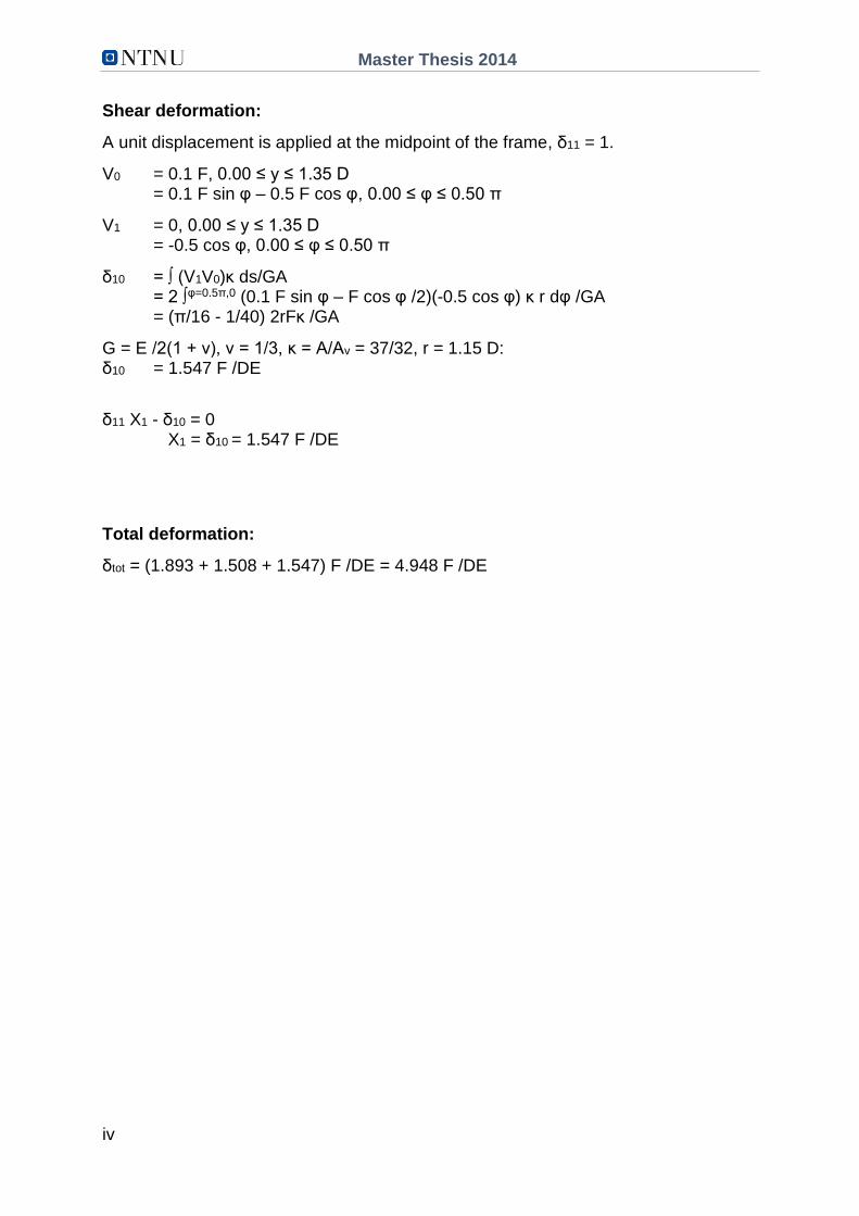
Master Thesis 2014

iv

Shear deformation:


V0 = 0.1 F, 0.00 ≤ y ≤ 1.35 D = 0.1 F sin φ – 0.5 F cos φ , 0.00 ≤ φ ≤ 0.50 π

V1 = 0, 0.00 ≤ y ≤ 1.35 D = -0.5 cos φ, 0.00 ≤ φ ≤ 0.50 π

δ10 = ∫ (V1V0)κ ds/GA = 2 ∫φ=0.5π,0 (0.1 F sin φ – F cos φ /2)(-0.5 cos φ) κ r dφ /GA = (π/16 - 1/40) 2rFκ /GA

G = E /2(1 + ν), ν = 1/3, κ = A/Av = 37/32, r = 1.15 D: δ10 = 1.547 F /DE

δ11 X1 - δ10 = 0 X1 = δ10 = 1.547 F /DE

Total deformation:

δtot = (1.893 + 1.508 + 1.547) F /DE = 4.948 F /DE

Master Thesis 2014

v

B. Von Mises Yield Criterion

The highest normal stress at the inner side of the crown is combined with the shear

stress in a distance of 0.8 R from the centroid of the cross section. The stresses are

taken from the midpoint of the frame where the largest bending moment occurs.

ŕ = 1.15 D

R = D2/8 (ŕ - √( ŕ2 – 0.25 D2)) = 1.0928 D

y = R – r1

youter = -0.5572 D

yinner = 0.4428 D

M = -0.325 FD

e = ŕ – R = 0.0572 D

𝜎𝑏 =𝑀(𝑅−𝑟1)

𝐴 𝑟1(ŕ−𝑅)

σb,outer = -0.325 FD (-0.5572 D)/(π 0.25 D2 0.0572 D 1.65 D) = 2.44 F/D2

σb.inner = -0.325 FD 0.4428 D/( π 0.25 D2 0.0572 D 0.65 D) = -4.93 F/D2

N = 0.1 F

𝜎 =𝑁

𝐴+

𝑀(𝑅−𝑟1)

𝐴 𝑟1(ŕ−𝑅)

σouter = (0.1 F/π 0.25 D2) + 2.44 F/D2 = 2.57 F/D2 σinner = (0.1 F/π 0.25 D2) – 4.93 F/D2 = -4.80 F/D2

V = F/2 S and t are determined in a distance of 0.8 times the cross-sectional radius from the centroid of the cross section: S = A y ≈ 0.0818 R2 0.8667 R = 0.0709 R3 t = 1.2 R

𝜏𝐸𝑑 =𝑉𝐸𝑑 𝑆

𝐼 𝑡≤

𝑓𝑦𝑑

√3

τ0.8R ≈ F 0.0709 R3/(2 0.25 π R4 1.2 R) = 0.47 F/D2

The Von Mises yield criterion:

(𝜎𝑥,𝐸𝑑

𝑓𝑦𝑑)

2

+ (𝜎𝑧,𝐸𝑑

𝑓𝑦𝑑)

2

− (𝜎𝑥,𝐸𝑑

𝑓𝑦𝑑) (

𝜎𝑧,𝐸𝑑

𝑓𝑦𝑑) + 3 (

𝜏𝐸𝑑

𝑓𝑦𝑑)

2

≤ 1

Steel grade R3: fy = 410 MPa

fu = 690 MPa

√[(4.80 F/D2)2 + 3 (0.47 F/D2)2] ≤ 410/1.05 F ≤ 80.21 D2

Master Thesis 2014

vi

Corrected M-/V- and N-values as a result of uniformly distributed load equal

to F/D instead of point load F and a whole chain link instead of half a chain link

provides the following corrected values at the midpoint of the frame:

Mcorr. ≈ -0.300 FD ∙ (0.223/0.328) = -0.204 FD

Vcorr. ≈ 0.00

Ncorr. ≈ 0.10 F

These values may apply to stud chain links.

σb,outer = -0.204 FD (-0.5572 D)/(π 0.25 D2 0.0572 D 1.65 D) = 1.53 F/D2

σb.inner = -0.204 FD 0.4428 D/( π 0.25 D2 0.0572 D 0.65 D) = -3.09 F/D2

σouter = (0.1 F/π 0.25 D2) + 1.53 F/D2 = 1.66 F/D2

σinner = (0.1 F/π 0.25 D2) – 3.09 F/D2 = -2.96 F/D2

√(2.96 F/D2)2 ≤ 410/1.05 F ≤ 131.9 D2

Master Thesis 2014

vii

C. Plastic Capacity

Corrected M-/V- and N-values as a result of uniformly distributed load equal

to F/D instead of point load F and a whole chain link instead of half a chain link

provides the following corrected values at the midpoint of the frame:

Mcorr. ≈ -0.300 FD ∙ (0.223/0.328) = -0.204 FD

Vcorr. ≈ 0.00

Ncorr. ≈ 0.10 F

These values may apply to stud chain links.

Interaction formula for interaction between axial load and bending:

𝑀𝐸𝑑 ≤ 𝑀𝑁,𝑅𝑑 = 𝑀𝑝𝑙,𝑅𝑑[1 − (𝑁𝐸𝑑/𝑁𝑝𝑙,𝑅𝑑)2]

Steel grade R3: fy = 410 MPa

fu = 690 MPa

0.204 FD ≤ (4/3) (D/2)3 410/1.05 [1 – (0.1 F/π (D/2)2 (410/1.05))2]

0.204 FD ≤ 65.079 D3 [1 – (0.1 F/306.679 D2)2]

0.204 FD ≤ 65.079 D3 – 6.919 10-6 F2/D

6.919 10-6 F2 + 0.204 FD2 – 65.079 D4 ≤ 0

D = 100 mm:

F ≤ 3150 kN

Chain in Mooring System

Documents

mooring chains

mooring systems kjettinger

mooring line failure

fortyningssystemer chains

chain links

stud links

studless links

worn links