Ch.8 Exercises: Tree Based Methods

Ch.8 Exercises: Tree Based Methods

1.

2.

• When using boosting with depth=1, each model consists of a single split created using one distinctvariable. So the total number of decision trees(B) is the same as the number of predictors(p); 𝐵 = 𝑝 inthis case. A new model is fit on the residuals left over from the previous model, and the new model’soutput is then added to the previous models. Therefore, the final model is additive.

3.

• ̂𝑝𝑚𝑘 : Proportion of training observations in the 𝑚𝑡ℎ region from the 𝑘𝑡ℎ class.

• Therefore, in a setting with two classes (k=2), ̂𝑝𝑚1 = 1 − ̂𝑝𝑚2.

• Classification Error Rate E when 1 > ̂𝑝𝑚1 > 0.5(Class 1 is most common class): 𝐸 = 1 − ̂𝑝𝑚1

• E when 0 < ̂𝑝𝑚1 < 0.5 (Class 1 is least common class): 𝐸 = 1 − ̂𝑝𝑚2 = 1 − (1 − ̂𝑝𝑚1)

• Gini index (G) takes a small value when ̂𝑝𝑚𝑘 is near 0 or 1.

• Gini index in terms of ̂𝑝𝑚1 is: 𝐺 = 2 ̂𝑝𝑚1(1 − ̂𝑝𝑚1).

• Cross entropy (D) is: 𝐷 = − ̂𝑝𝑚1 log ̂𝑝𝑚1 − (1 − ̂𝑝𝑚1) log(1 − ̂𝑝𝑚1).

1

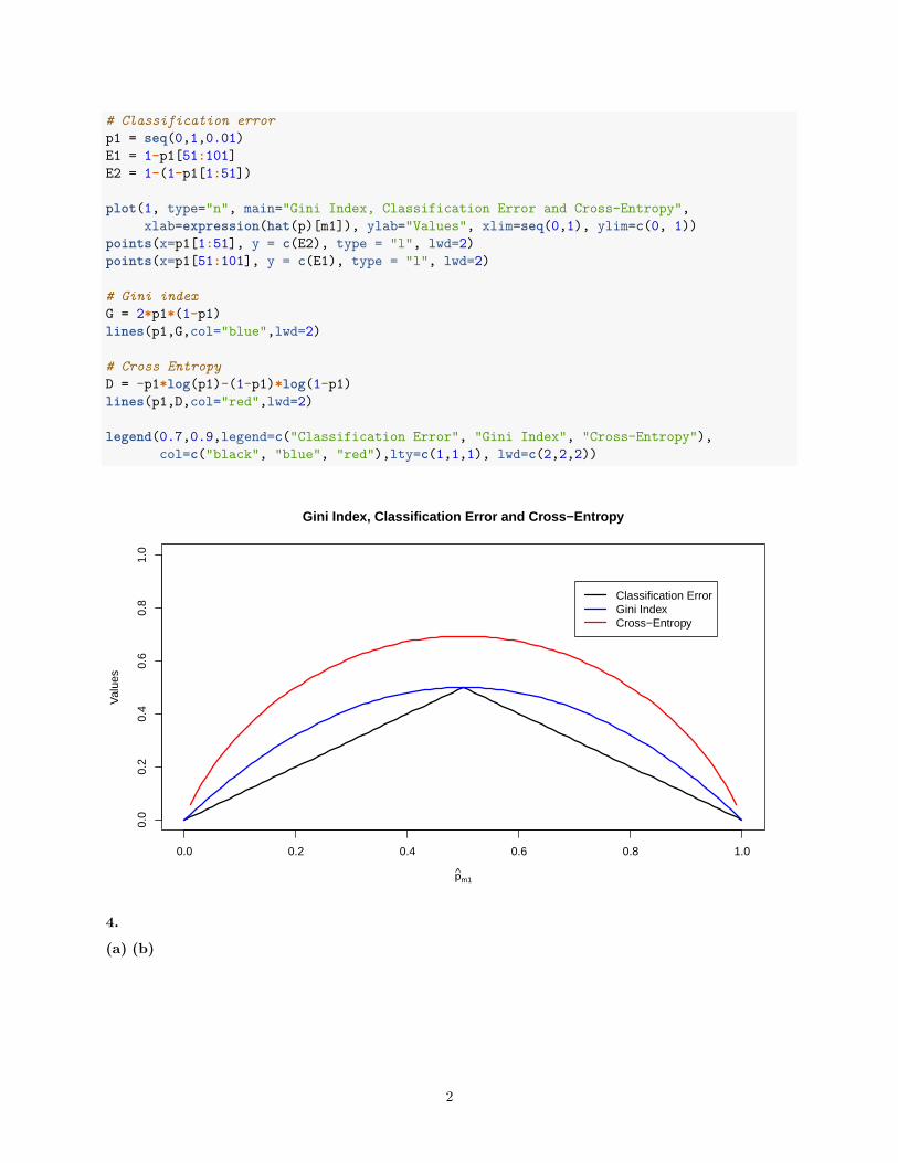
# Classification errorp1 = seq(0,1,0.01)E1 = 1-p1[51:101]E2 = 1-(1-p1[1:51])

plot(1, type="n", main="Gini Index, Classification Error and Cross-Entropy",xlab=expression(hat(p)[m1]), ylab="Values", xlim=seq(0,1), ylim=c(0, 1))

points(x=p1[1:51], y = c(E2), type = "l", lwd=2)points(x=p1[51:101], y = c(E1), type = "l", lwd=2)

# Gini indexG = 2*p1*(1-p1)lines(p1,G,col="blue",lwd=2)

# Cross EntropyD = -p1*log(p1)-(1-p1)*log(1-p1)lines(p1,D,col="red",lwd=2)

legend(0.7,0.9,legend=c("Classification Error", "Gini Index", "Cross-Entropy"),col=c("black", "blue", "red"),lty=c(1,1,1), lwd=c(2,2,2))

0.0 0.2 0.4 0.6 0.8 1.0

0.0

0.2

0.4

0.6

0.8

1.0

Gini Index, Classification Error and Cross−Entropy

p̂m1

Val

ues

Classification ErrorGini IndexCross−Entropy

4.

(a) (b)

2

5.

Majority voting for classification:

• Count of P(Class is Red | X) < 0.5 = 4 and P(Class is Red | X) >= 0.5 = 6. So X is classifiedas red.

Average probability:

• Average probability that P(Class is Red | X) is 4.5/10 = 0.45. Therefore, X is classified as green.

6.

The algorithm grows a very large tree 𝑇0 using recursive binary splitting to minimise the RSS. It stopsgrowing when a terminal node has has fewer than some minimum number of observations.𝑇0 due to its sizeand complexity can overfit the data. As such a tree ‘pruning’ process is applied to 𝑇0 that returns subtreesas a function of 𝛼 (a positive tuning parameter).Each value of 𝛼 results in a tree 𝑇 that is a subset of 𝑇0which minimizes the quantity (8.4).

Thereafter, K-fold cross-validation is used to select the best value of 𝛼, by evaluating the predictions fromtrees on the test set. The value of 𝛼 that gives the lowest test MSE is selected.

Finally, the best value of 𝛼 is used to prune T. This will return the tree corresponding to that 𝛼.

Applied

library(MASS)library(randomForest)require(caTools)library(ISLR)library(tree)library(tidyr)library(glmnet) #Ridge Regression and Lassolibrary(gbm) #Boosting

3

7.

# Train and test sets with their respective Y responses.set.seed(1)df = Bostonsample.data = sample.split(df$medv, SplitRatio = 0.70)train.set = subset(df, select=-c(medv), sample.data==T) #Using select to drop medv(Y) column.test.set = subset(df, select=-c(medv), sample.data==F)train.Y = subset(df$medv, sample.data==T)test.Y = subset(df$medv, sample.data==F)

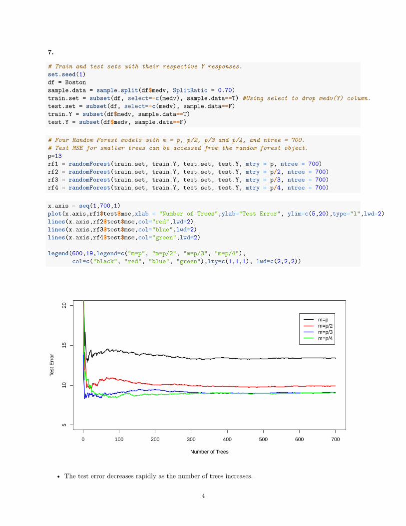
# Four Random Forest models with m = p, p/2, p/3 and p/4, and ntree = 700.# Test MSE for smaller trees can be accessed from the random forest object.p=13rf1 = randomForest(train.set, train.Y, test.set, test.Y, mtry = p, ntree = 700)rf2 = randomForest(train.set, train.Y, test.set, test.Y, mtry = p/2, ntree = 700)rf3 = randomForest(train.set, train.Y, test.set, test.Y, mtry = p/3, ntree = 700)rf4 = randomForest(train.set, train.Y, test.set, test.Y, mtry = p/4, ntree = 700)

x.axis = seq(1,700,1)plot(x.axis,rf1$test$mse,xlab = "Number of Trees",ylab="Test Error", ylim=c(5,20),type="l",lwd=2)lines(x.axis,rf2$test$mse,col="red",lwd=2)lines(x.axis,rf3$test$mse,col="blue",lwd=2)lines(x.axis,rf4$test$mse,col="green",lwd=2)

legend(600,19,legend=c("m=p", "m=p/2", "m=p/3", "m=p/4"),col=c("black", "red", "blue", "green"),lty=c(1,1,1), lwd=c(2,2,2))

0 100 200 300 400 500 600 700

510

1520

Number of Trees

Test

Err

or

m=pm=p/2m=p/3m=p/4

• The test error decreases rapidly as the number of trees increases.

4

• The test error gets lower as m decreases from m=p upto m=p/3, and thereafter we find no significantchanges.

8. (a) (b)

set.seed(2)

df = Carseatssample.data = sample.split(df$Sales, SplitRatio = 0.70)

train.set = subset(df, sample.data==T)test.set = subset(df, sample.data==F)

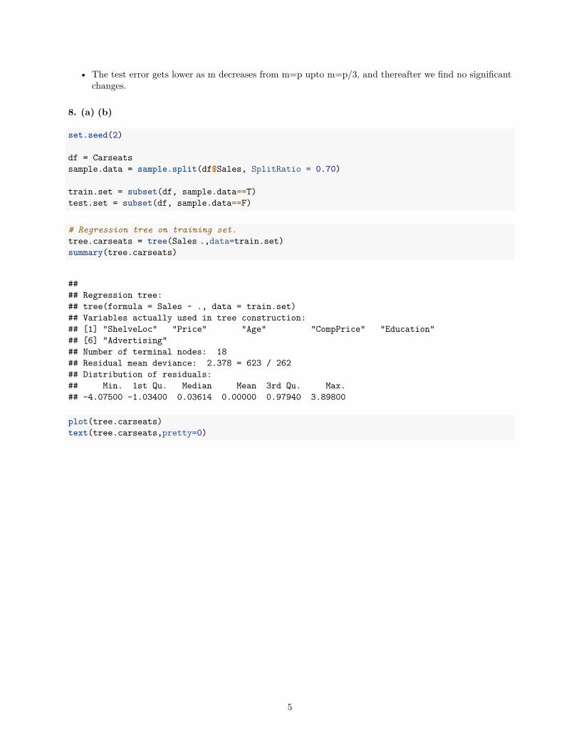
# Regression tree on training set.tree.carseats = tree(Sales�.,data=train.set)summary(tree.carseats)

#### Regression tree:## tree(formula = Sales ~ ., data = train.set)## Variables actually used in tree construction:## [1] "ShelveLoc" "Price" "Age" "CompPrice" "Education"## [6] "Advertising"## Number of terminal nodes: 18## Residual mean deviance: 2.378 = 623 / 262## Distribution of residuals:## Min. 1st Qu. Median Mean 3rd Qu. Max.## -4.07500 -1.03400 0.03614 0.00000 0.97940 3.89800

plot(tree.carseats)text(tree.carseats,pretty=0)

5

|ShelveLoc: Bad,Medium

Price < 105.5

ShelveLoc: Bad

Age < 68.5CompPrice < 118.5

Age < 50.5

ShelveLoc: Bad

Price < 132.5CompPrice < 136

Age < 47.5

Education < 16.5 Advertising < 13.5Price < 137

Price < 109.5

Advertising < 13.5

Price < 144Age < 59.5

6.833 10.060 5.066 10.530 8.592

4.528 7.251 3.219

8.086 6.137 5.884 4.075

7.234

12.590

10.570 8.419 6.566

12.270

# Test MSE.tree.pred = predict(tree.carseats,test.set)test.mse = mean((tree.pred-test.set$Sales)^2)test.mse

## [1] 4.974844

• Shelve location and Price are the most important predictors, same as with the classification tree.• Test MSE is: 4.98

(c)

set.seed(2)cv.carseats = cv.tree(tree.carseats)plot(cv.carseats$size,cv.carseats$dev,xlab="Terminal Nodes",ylab="CV Error",type="b")

6

5 10 15

1400

1800

2200

Terminal Nodes

CV

Err

or

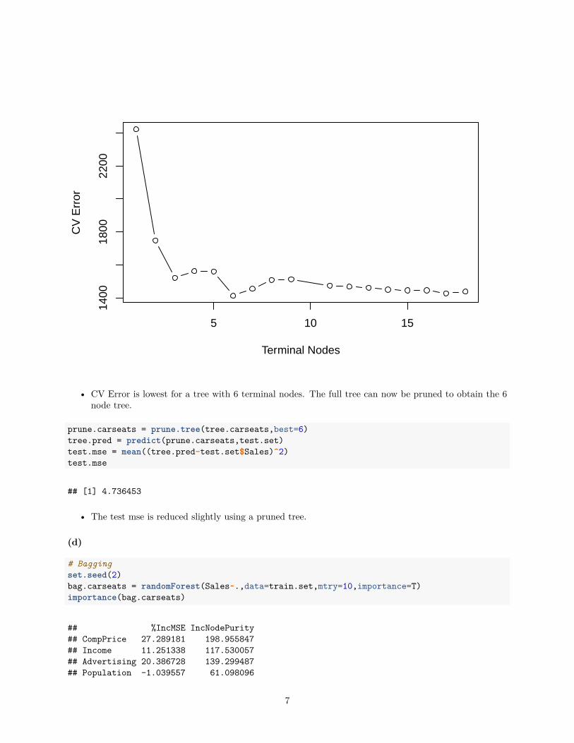
• CV Error is lowest for a tree with 6 terminal nodes. The full tree can now be pruned to obtain the 6node tree.

prune.carseats = prune.tree(tree.carseats,best=6)tree.pred = predict(prune.carseats,test.set)test.mse = mean((tree.pred-test.set$Sales)^2)test.mse

## [1] 4.736453

• The test mse is reduced slightly using a pruned tree.

(d)

# Baggingset.seed(2)bag.carseats = randomForest(Sales~.,data=train.set,mtry=10,importance=T)importance(bag.carseats)

## %IncMSE IncNodePurity## CompPrice 27.289181 198.955847## Income 11.251338 117.530057## Advertising 20.386728 139.299487## Population -1.039557 61.098096

7

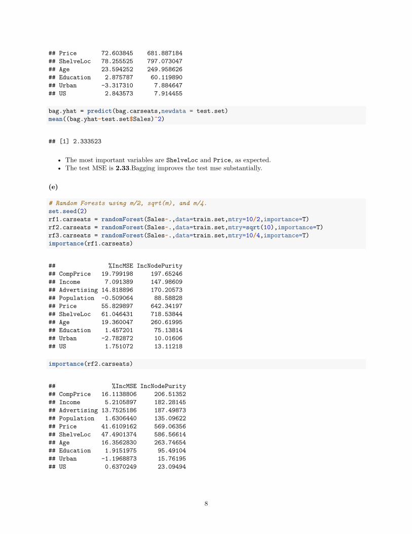
## Price 72.603845 681.887184## ShelveLoc 78.255525 797.073047## Age 23.594252 249.958626## Education 2.875787 60.119890## Urban -3.317310 7.884647## US 2.843573 7.914455

bag.yhat = predict(bag.carseats,newdata = test.set)mean((bag.yhat-test.set$Sales)^2)

## [1] 2.333523

• The most important variables are ShelveLoc and Price, as expected.• The test MSE is 2.33.Bagging improves the test mse substantially.

(e)

# Random Forests using m/2, sqrt(m), and m/4.set.seed(2)rf1.carseats = randomForest(Sales~.,data=train.set,mtry=10/2,importance=T)rf2.carseats = randomForest(Sales~.,data=train.set,mtry=sqrt(10),importance=T)rf3.carseats = randomForest(Sales~.,data=train.set,mtry=10/4,importance=T)importance(rf1.carseats)

## %IncMSE IncNodePurity## CompPrice 19.799198 197.65246## Income 7.091389 147.98609## Advertising 14.818896 170.20573## Population -0.509064 88.58828## Price 55.829897 642.34197## ShelveLoc 61.046431 718.53844## Age 19.360047 260.61995## Education 1.457201 75.13814## Urban -2.782872 10.01606## US 1.751072 13.11218

importance(rf2.carseats)

## %IncMSE IncNodePurity## CompPrice 16.1138806 206.51352## Income 5.2105897 182.28145## Advertising 13.7525186 187.49873## Population 1.6306440 135.09622## Price 41.6109162 569.06356## ShelveLoc 47.4901374 586.56614## Age 16.3562830 263.74654## Education 1.9151975 95.49104## Urban -1.1968873 15.76195## US 0.6370249 23.09494

8

importance(rf3.carseats)

## %IncMSE IncNodePurity## CompPrice 10.5760361 209.09892## Income 3.1052773 197.09133## Advertising 11.3311914 190.61102## Population -0.3444876 167.52584## Price 38.9378885 506.67890## ShelveLoc 39.0090484 501.09857## Age 15.3092988 259.83685## Education 0.1770255 109.99735## Urban -0.2056953 23.96764## US 2.6623260 30.13254

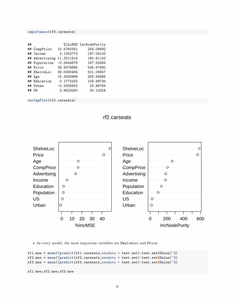
varImpPlot(rf2.carseats)

UrbanUSPopulationEducationIncomeAdvertisingCompPriceAgePriceShelveLoc

0 10 20 30 40%IncMSE

UrbanUSEducationPopulationIncomeAdvertisingCompPriceAgePriceShelveLoc

0 200 400 600IncNodePurity

rf2.carseats

• In every model, the most important variables are ShelveLoc and Price.

rf1.mse = mean((predict(rf1.carseats,newdata = test.set)-test.set$Sales)^2)rf2.mse = mean((predict(rf2.carseats,newdata = test.set)-test.set$Sales)^2)rf3.mse = mean((predict(rf3.carseats,newdata = test.set)-test.set$Sales)^2)

rf1.mse;rf2.mse;rf3.mse

9

## [1] 2.196814

## [1] 2.410541

## [1] 2.61837

• Test MSE using random forest with m=p/2 is 2.2,and this is slightly lower than using bagging.

9. (a) (b) (c) (d)

#dim(OJ)set.seed(3)

df = OJsample.data = sample.split(df$Purchase, SplitRatio = 800/1070) #800 observations for the test set.train.set = subset(df, sample.data==T)test.set = subset(df, sample.data==F)

tree.OJ = tree(Purchase�.,data=train.set)summary(tree.OJ)

#### Classification tree:## tree(formula = Purchase ~ ., data = train.set)## Variables actually used in tree construction:## [1] "LoyalCH" "WeekofPurchase" "PriceDiff" "ListPriceDiff"## [5] "PctDiscMM"## Number of terminal nodes: 10## Residual mean deviance: 0.6798 = 537 / 790## Misclassification error rate: 0.15 = 120 / 800

• The training error rate is 0.15, and there are 10 terminal nodes.• The residual mean deviance is high, and so this model doesn’t provide a good fit to the training data.

tree.OJ

## node), split, n, deviance, yval, (yprob)## * denotes terminal node#### 1) root 800 1070.000 CH ( 0.61000 0.39000 )## 2) LoyalCH < 0.469289 300 313.600 MM ( 0.21667 0.78333 )## 4) LoyalCH < 0.276142 173 111.200 MM ( 0.09827 0.90173 )## 8) WeekofPurchase < 238.5 49 0.000 MM ( 0.00000 1.00000 ) *## 9) WeekofPurchase > 238.5 124 99.120 MM ( 0.13710 0.86290 )## 18) LoyalCH < 0.0356415 55 9.996 MM ( 0.01818 0.98182 ) *## 19) LoyalCH > 0.0356415 69 74.730 MM ( 0.23188 0.76812 ) *## 5) LoyalCH > 0.276142 127 168.400 MM ( 0.37795 0.62205 )## 10) PriceDiff < 0.05 56 55.490 MM ( 0.19643 0.80357 ) *## 11) PriceDiff > 0.05 71 98.300 CH ( 0.52113 0.47887 )## 22) LoyalCH < 0.308433 9 0.000 CH ( 1.00000 0.00000 ) *## 23) LoyalCH > 0.308433 62 85.370 MM ( 0.45161 0.54839 ) *

10

## 3) LoyalCH > 0.469289 500 429.600 CH ( 0.84600 0.15400 )## 6) LoyalCH < 0.764572 240 289.700 CH ( 0.70833 0.29167 )## 12) ListPriceDiff < 0.235 100 138.500 CH ( 0.52000 0.48000 )## 24) PctDiscMM < 0.196197 81 108.700 CH ( 0.60494 0.39506 ) *## 25) PctDiscMM > 0.196197 19 16.570 MM ( 0.15789 0.84211 ) *## 13) ListPriceDiff > 0.235 140 121.800 CH ( 0.84286 0.15714 ) *## 7) LoyalCH > 0.764572 260 64.420 CH ( 0.97308 0.02692 ) *

• Branch 8 results in a terminal node. The split criterion is WeekofPurchase < 238.5 and there are 49observations in this branch, with each observation belonging to MM. Therefore, the final predictionfor this branch is MM.

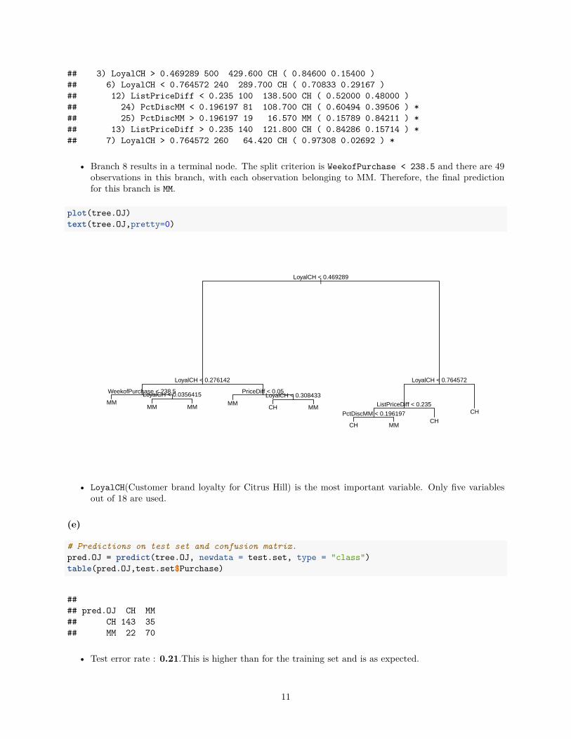
plot(tree.OJ)text(tree.OJ,pretty=0)

|LoyalCH < 0.469289

LoyalCH < 0.276142

WeekofPurchase < 238.5LoyalCH < 0.0356415 PriceDiff < 0.05LoyalCH < 0.308433

LoyalCH < 0.764572

ListPriceDiff < 0.235

PctDiscMM < 0.196197

MMMM MM

MMCH MM

CH MMCH

CH

• LoyalCH(Customer brand loyalty for Citrus Hill) is the most important variable. Only five variablesout of 18 are used.

(e)

# Predictions on test set and confusion matrix.pred.OJ = predict(tree.OJ, newdata = test.set, type = "class")table(pred.OJ,test.set$Purchase)

#### pred.OJ CH MM## CH 143 35## MM 22 70

• Test error rate : 0.21.This is higher than for the training set and is as expected.

11

(f) (g) (h)

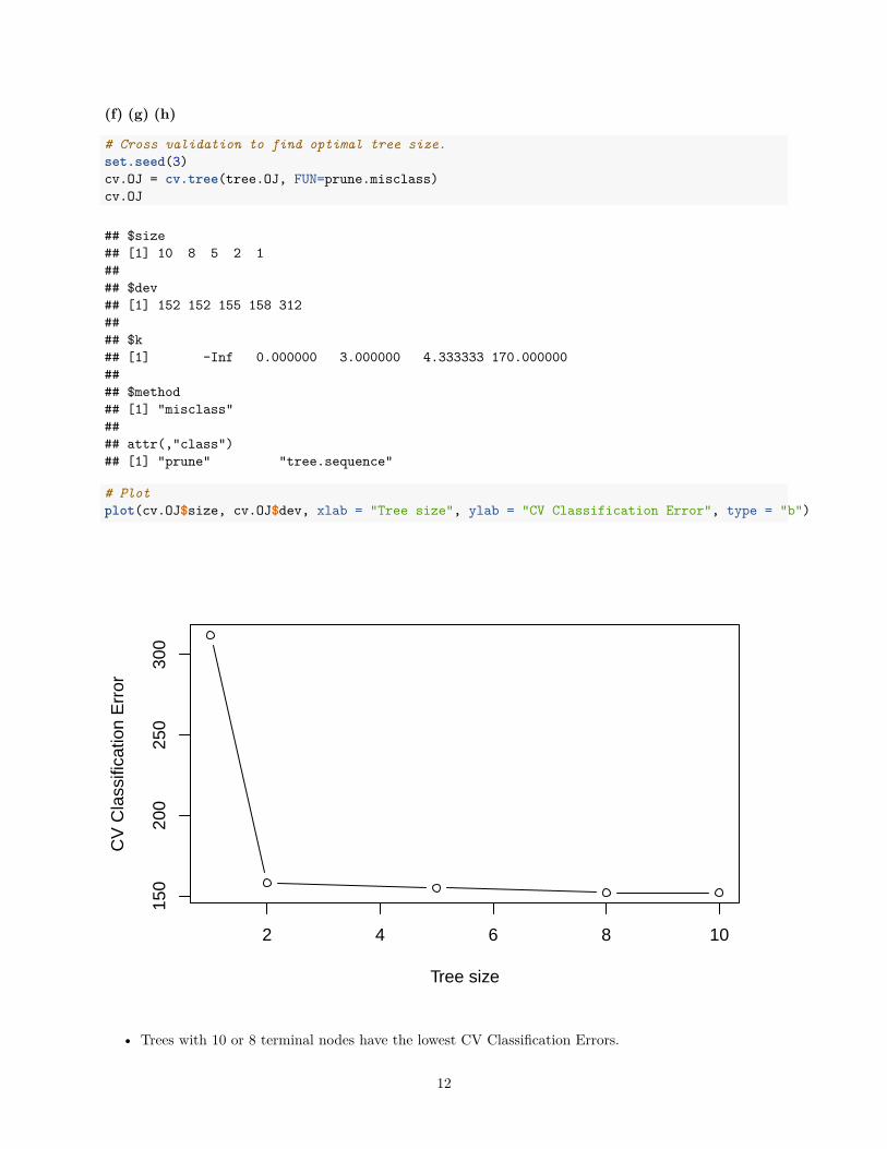
# Cross validation to find optimal tree size.set.seed(3)cv.OJ = cv.tree(tree.OJ, FUN=prune.misclass)cv.OJ

## $size## [1] 10 8 5 2 1#### $dev## [1] 152 152 155 158 312#### $k## [1] -Inf 0.000000 3.000000 4.333333 170.000000#### $method## [1] "misclass"#### attr(,"class")## [1] "prune" "tree.sequence"

# Plotplot(cv.OJ$size, cv.OJ$dev, xlab = "Tree size", ylab = "CV Classification Error", type = "b")

2 4 6 8 10

150

200

250

300

Tree size

CV

Cla

ssifi

catio

n E

rror

• Trees with 10 or 8 terminal nodes have the lowest CV Classification Errors.

12

(i) (j)

# Tree with five terminal nodes and training error.prune.OJ = prune.misclass(tree.OJ,best=5)pred.prune = predict(prune.OJ, newdata = train.set, type = "class")table(pred.prune,train.set$Purchase)

#### pred.prune CH MM## CH 420 61## MM 68 251

• Training error rate : 0.16. Slightly higher than using the full tree.

(k)

pred.prune = predict(prune.OJ, newdata = test.set, type = "class")table(pred.prune,test.set$Purchase)

#### pred.prune CH MM## CH 143 34## MM 22 71

• Test error rate : 0.207. Pretty much the same as using the full tree, however, we now have a moreinterpretable tree.

10.

(a) (b)

# NA values dropped from Salary, and Log transform.Hitters = Hitters %>% drop_na(Salary)Hitters$Salary = log(Hitters$Salary)

# Training and test sets with 200 and 63 observations respectively.set.seed(4)sample.data = sample.split(Hitters$Salary, SplitRatio = 200/263)train.set = subset(Hitters, sample.data==T)test.set = subset(Hitters, sample.data==F)

(c) (d)

# Boosting with 1000 trees for a range of lambda values, and computing the training and test mse.lambdas = seq(0.0001,0.5,0.01)train.mse = rep(NA,length(lambdas))test.mse = rep(NA,length(lambdas))

set.seed(4)for (i in lambdas){boost.Hitters = gbm(Salary~., data=train.set,distribution = "gaussian", n.trees = 1000,

13

interaction.depth = 4, shrinkage = i)yhat.train = predict(boost.Hitters,newdata = train.set, n.trees = 1000)train.mse[which(i==lambdas)] = mean((yhat.train-train.set$Salary)^2)

yhat.test = predict(boost.Hitters,newdata = test.set, n.trees = 1000)test.mse[which(i==lambdas)] = mean((yhat.test-test.set$Salary)^2)

}

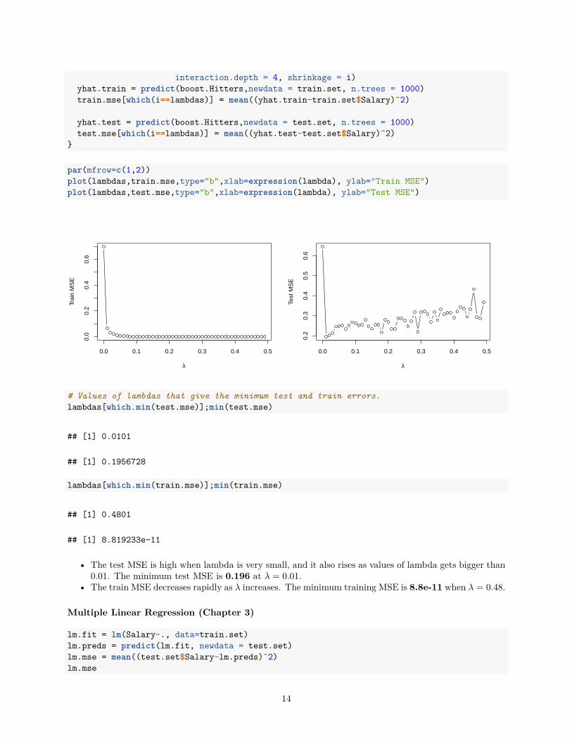
par(mfrow=c(1,2))plot(lambdas,train.mse,type="b",xlab=expression(lambda), ylab="Train MSE")plot(lambdas,test.mse,type="b",xlab=expression(lambda), ylab="Test MSE")

0.0 0.1 0.2 0.3 0.4 0.5

0.0

0.2

0.4

0.6

λ

Trai

n M

SE

0.0 0.1 0.2 0.3 0.4 0.5

0.2

0.3

0.4

0.5

0.6

λ

Test

MS

E

# Values of lambdas that give the minimum test and train errors.lambdas[which.min(test.mse)];min(test.mse)

## [1] 0.0101

## [1] 0.1956728

lambdas[which.min(train.mse)];min(train.mse)

## [1] 0.4801

## [1] 8.819233e-11

• The test MSE is high when lambda is very small, and it also rises as values of lambda gets bigger than0.01. The minimum test MSE is 0.196 at 𝜆 = 0.01.

• The train MSE decreases rapidly as 𝜆 increases. The minimum training MSE is 8.8e-11 when 𝜆 = 0.48.

Multiple Linear Regression (Chapter 3)

lm.fit = lm(Salary~., data=train.set)lm.preds = predict(lm.fit, newdata = test.set)lm.mse = mean((test.set$Salary-lm.preds)^2)lm.mse

14

## [1] 0.412438

Lasso model (Chapter 6)

# Matrix of training and test sets, and their respective responses.train = model.matrix(Salary~.,train.set)test = model.matrix(Salary~.,test.set)y.train = train.set$Salarylasso.mod = glmnet(train, y.train, alpha = 1)

# Cross validation to select best lambda.set.seed(4)cv.out=cv.glmnet(train, y.train, alpha=1)bestlam=cv.out$lambda.minlasso.pred=predict(lasso.mod, s=bestlam, newx = test)mean((test.set$Salary-lasso.pred)^2)

## [1] 0.3335934

• The test MSE of Multiple Linear Regression and the Lasso is 0.41 and 0.33 respectively.• The test MSE of boosting is 0.20, which is lower than both.

(f)

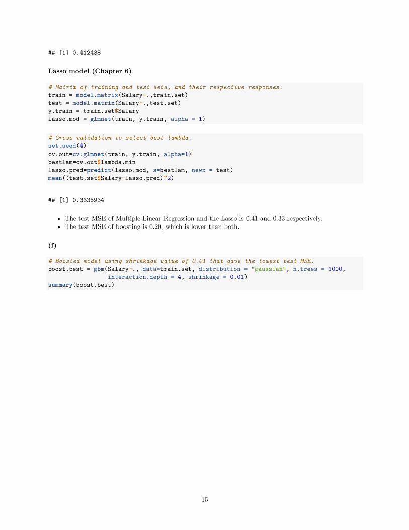
# Boosted model using shrinkage value of 0.01 that gave the lowest test MSE.boost.best = gbm(Salary~., data=train.set, distribution = "gaussian", n.trees = 1000,

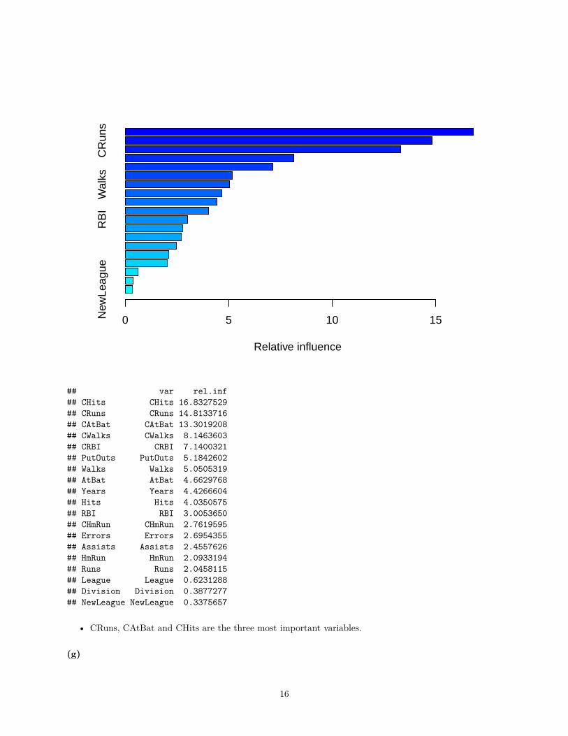
interaction.depth = 4, shrinkage = 0.01)summary(boost.best)

15

New

Leag

ueR

BI

Wal

ksC

Run

s

Relative influence

0 5 10 15

## var rel.inf## CHits CHits 16.8327529## CRuns CRuns 14.8133716## CAtBat CAtBat 13.3019208## CWalks CWalks 8.1463603## CRBI CRBI 7.1400321## PutOuts PutOuts 5.1842602## Walks Walks 5.0505319## AtBat AtBat 4.6629768## Years Years 4.4266604## Hits Hits 4.0350575## RBI RBI 3.0053650## CHmRun CHmRun 2.7619595## Errors Errors 2.6954355## Assists Assists 2.4557626## HmRun HmRun 2.0933194## Runs Runs 2.0458115## League League 0.6231288## Division Division 0.3877277## NewLeague NewLeague 0.3375657

• CRuns, CAtBat and CHits are the three most important variables.

(g)

16

bag.Hitters = randomForest(Salary~.,train.set,mtry=19,importance=T)bag.pred = predict(bag.Hitters,newdata = test.set)mean((test.set$Salary-bag.pred)^2)

## [1] 0.1905075

• The test MSE using bagging is 0.191, and this is slightly lower than from boosting.

11.

(a)

#Creating Purchase01 column and adding 1 if Purchase is "Yes" and 0 if "No".Caravan$Purchase01=rep(NA,5822)for (i in 1:5822) if (Caravan$Purchase[i] == "Yes")(Caravan$Purchase01[i]=1) else (Caravan$Purchase01[i]=0)

# Training set consisting of first 1000 observations, and the test set from the rest.train.set = Caravan[1:1000,]test.set = Caravan[1001:5822,]

(b)

# Boosting model for classification.set.seed(5)boost.Caravan = gbm(Purchase01~.-Purchase, data=train.set,distribution = "bernoulli",

n.trees = 1000, shrinkage = 0.01)

## Warning in gbm.fit(x = x, y = y, offset = offset, distribution = distribution, :## variable 50: PVRAAUT has no variation.

## Warning in gbm.fit(x = x, y = y, offset = offset, distribution = distribution, :## variable 71: AVRAAUT has no variation.

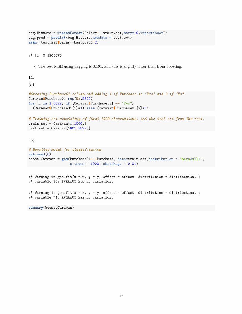
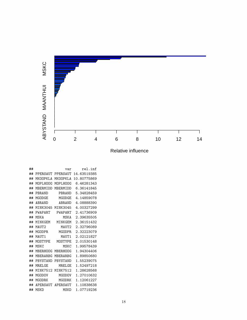
summary(boost.Caravan)

17

AB

YS

TAN

DM

AA

NT

HU

IM

SK

C

Relative influence

0 2 4 6 8 10 12 14

## var rel.inf## PPERSAUT PPERSAUT 14.63519385## MKOOPKLA MKOOPKLA 10.80775869## MOPLHOOG MOPLHOOG 6.46281343## MBERMIDD MBERMIDD 6.36141845## PBRAND PBRAND 5.34828459## MGODGE MGODGE 4.14859078## ABRAND ABRAND 4.08888390## MINK3045 MINK3045 4.00327299## PWAPART PWAPART 2.41736909## MSKA MSKA 2.39635505## MINKGEM MINKGEM 2.36151432## MAUT2 MAUT2 2.32796089## MGODPR MGODPR 2.32223079## MAUT1 MAUT1 2.02121827## MOSTYPE MOSTYPE 2.01530148## MSKC MSKC 1.99578439## MBERHOOG MBERHOOG 1.94304406## MBERARBG MBERARBG 1.89850680## PBYSTAND PBYSTAND 1.55239075## MRELGE MRELGE 1.52497218## MINK7512 MINK7512 1.28628568## MGODOV MGODOV 1.27010632## MGODRK MGODRK 1.12061227## APERSAUT APERSAUT 1.10838638## MSKD MSKD 1.07719236

18

## MSKB1 MSKB1 1.07315282## MOPLMIDD MOPLMIDD 1.03311174## MAUT0 MAUT0 0.95142058## MINKM30 MINKM30 0.94409509## MFWEKIND MFWEKIND 0.91979519## MFGEKIND MFGEKIND 0.91420410## MINK4575 MINK4575 0.83510909## MRELOV MRELOV 0.72566461## MOSHOOFD MOSHOOFD 0.60620604## MHHUUR MHHUUR 0.60380352## MHKOOP MHKOOP 0.56934690## MBERBOER MBERBOER 0.52970179## MZPART MZPART 0.51652596## MBERARBO MBERARBO 0.48041153## PMOTSCO PMOTSCO 0.46916473## PLEVEN PLEVEN 0.42654929## MGEMLEEF MGEMLEEF 0.39318771## MGEMOMV MGEMOMV 0.32657396## MRELSA MRELSA 0.32447332## MZFONDS MZFONDS 0.28439837## MOPLLAAG MOPLLAAG 0.20951055## MSKB2 MSKB2 0.15533586## MINK123M MINK123M 0.14129531## MFALLEEN MFALLEEN 0.07151417## MAANTHUI MAANTHUI 0.00000000## MBERZELF MBERZELF 0.00000000## PWABEDR PWABEDR 0.00000000## PWALAND PWALAND 0.00000000## PBESAUT PBESAUT 0.00000000## PVRAAUT PVRAAUT 0.00000000## PAANHANG PAANHANG 0.00000000## PTRACTOR PTRACTOR 0.00000000## PWERKT PWERKT 0.00000000## PBROM PBROM 0.00000000## PPERSONG PPERSONG 0.00000000## PGEZONG PGEZONG 0.00000000## PWAOREG PWAOREG 0.00000000## PZEILPL PZEILPL 0.00000000## PPLEZIER PPLEZIER 0.00000000## PFIETS PFIETS 0.00000000## PINBOED PINBOED 0.00000000## AWAPART AWAPART 0.00000000## AWABEDR AWABEDR 0.00000000## AWALAND AWALAND 0.00000000## ABESAUT ABESAUT 0.00000000## AMOTSCO AMOTSCO 0.00000000## AVRAAUT AVRAAUT 0.00000000## AAANHANG AAANHANG 0.00000000## ATRACTOR ATRACTOR 0.00000000## AWERKT AWERKT 0.00000000## ABROM ABROM 0.00000000## ALEVEN ALEVEN 0.00000000## APERSONG APERSONG 0.00000000## AGEZONG AGEZONG 0.00000000

19

## AWAOREG AWAOREG 0.00000000## AZEILPL AZEILPL 0.00000000## APLEZIER APLEZIER 0.00000000## AFIETS AFIETS 0.00000000## AINBOED AINBOED 0.00000000## ABYSTAND ABYSTAND 0.00000000

• PPERSAUT and MKOOPKLA appear to be the most important variables.

(c)

# Predcited probalbilites on Test Set.probs.Caravan = predict(boost.Caravan, newdata = test.set, n.trees = 1000, type="response")

# Predict "Yes" if estimated probability is greater than 20%.preds = rep("No",4822)preds[probs.Caravan>0.20]="Yes"

# Confusion matrixactual = test.set$Purchasetable(actual, preds)

## preds## actual No Yes## No 4410 123## Yes 254 35

• Overall, the boosted model makes correct predictions for 92.2% of the observations.

• The actual number of “No” is 94% and “Yes” is 6%, and so this is an imbalanced dataset. A modelsimply predicting “No” on each occasion would have made 94% of the predictions correctly. However,in this case we are more interested in predicting those who go on to purchase the insurance.

• The model predicts “Yes” 158 times, and it is correct on 35 of these predictions - so 22.2% of thosepredicted to purchase actually do so. This is much better than random guessing (6%).

Comparing results with Logistic Regression

glm.fit = glm(Purchase~.-Purchase01, data = train.set, family = binomial)

## Warning: glm.fit: fitted probabilities numerically 0 or 1 occurred

glm.probs = predict(glm.fit, test.set, type="response")

## Warning in predict.lm(object, newdata, se.fit, scale = 1, type = if (type == :## prediction from a rank-deficient fit may be misleading

glm.preds = rep("No",4822)glm.preds[glm.probs>0.2]="Yes"table(actual,glm.preds)

20

## glm.preds## actual No Yes## No 4183 350## Yes 231 58

• Logistic regression predicts “Yes” 408 times, and it is correct on 58 occasions - so 14.2% of thosepredicted to purchase actually do so. This model is better than random guessing but is worse than theboosted model.

21