CAUSAL ANALYSIS WITH PANEL DATA - …users.cla.umn.edu/~uggen/Finkel_sage_1995_r.pdfCAUSAL ANALYSIS WITH PANEL DATA ACKNOWLEDGMENTS STEVEN E.FINKEL Department ofGovernmentandForeignAffairs

CAUSAL ANALYSISWITH PANEL DATA

ACKNOWLEDGMENTS STEVEN E. FINKELDepartment of Government and Foreign AffairsUniversity of Virginia

I would like to thank Charles E. Denk for his invaluable advice andencouragement at various stages of this project. Iam grateful to Denk, theseries editor Michael Lewis-Beck, several anonymous reviewers, Karl­Dieter Opp, Timothy S. Prinz, and Janet E. Steele for their careful critiquesand important suggestions for improving the manuscript. Ialso thank theUniversity of Virginia's Committee on Summer Grants and Center forAdvanced Studies for supporting this research during 1993-1994. Finally,the German data analyzed in the monograph were collected in collaborationwith Edward N. Muller and Karl-Dieter Opp with the support of theNational Science Foundation and the Stiftung Volkswagenwerk.

1. INTRODUCTION

Panel data, which consist of information gathered from the same individu­als or units at several different points in time, are commonly used in thesocial sciences to test theories of individual and social change. The mostimportant' feature of panel studies is that, in contrast to static cross­sectional analyses, change is explicitly incorporated into the design so thatindividual (or other unit-level) changes in a set of variables are directlymeasured. Panel data may also be distinguished from two other forms oflongitudinal data (Menard, 1991): "repeated cross-section" or "trend" data,which consist of information collected on the same variables for differentunits over time; and "time series" data, which consist of observationscollected on several variables for a single unit at multiple points in time(Ostrom, 1978). The distinctiveness of panel data is that they containmeasures of the same variables from numerous units observed repeatedlythrough time.1This monograph provides an overview of models appropriate for the

analysis of panel data, focusing specifically on the area where panels offermajor advantages over cross-sectional research designs: the analysis ofcausal interrelationships among variables. For a causal effect to exist fromvariable X to variable Y, the following well-known conditions must be met(Menard, 1991, p. 17): (a) Xand Ymust covary, as evidenced in nonexperi­mental studies by a nonzero bivariate correlation; (b) X must precede Yintime; and (c) the relationship must not be "spurious," or produced by X andY's joint association with a third variable or set of variables. Successfulcausal inference also depends on the accurate measurement of the variablesof interest because statistical estimation of causal effects will yield incor­rect results when random or nonrandom measurement errors in observedvariables are not taken into account (Berry & Feldman, 1985; Carmines &

vi

r2

Zeller, 1979). Cross-sectional data can provide evidence regarding the firstcondition of covariation, but their usefulness in providing evidence regard­ing time precedence and nonspuriousness, and in specifying models thatcorrect for measurement error in the variables, is much more limited. Aswill become evident, panel data offer decided advantages in all of theseareas.In cross-sectional analyses, the measurement of variables at a single time

point makes it difficult to establish temporal order, and hence to rule outthe possibility that covariation between X and Y is produced by Y causingX, or through a reciprocal causal relationship. By contrast, the observationof X and Y through time on the same units in panel analyses enables theresearcher to specify certain models that necessarily satisfy the timeprecedence criterion, that is, where prior values of each variable may affectlater values of the other. Further, in instances where reciprocal causality issuspected, the panel analyst may estimate nonrecursive models with feed­back effects between variables with fewer restrictive assumptions than inthe cross-sectional case. Panel data are also useful in controlling for theeffects of outside variables that may render the relationship between X andY either partially or fully spurious. Whereas spurious association in cross­sectional analysis can be tested only by actually including the outsidevariables in the statistical model, in panel studies certain patterns ofspuriousness caused by unmeasured factors may also be tested against thedata. Finally, measurement error models can be estimated with panel datawith fewer restrictive assumptions than are necessary in the cross-sectionalcontext, as the analyst can utilize the additional observations over time toestimate both causal effects and measurement properties of the variables.In all of these ways, panel designs allow more rigorous tests of causalrelations than are possible with cross-sections, and thus approximate moreclosely than other observational research designs the controlled testing ofcausality possible with experimental methods.Throughout the monograph, two complementary perspectives on causal

analysis with panel data will be presented. Itwill be shown that panel dataoffer multiple ways of strengthening the causal inference process, andsucceeding chapters will demonstrate how to estimate models that containa variety of lag specifications, reciprocal effects, and imperfectly measuredvariables. At the same time, it will be emphasized that panel data are not acure-all for the problems of causal inference in nonexperimental research.All of the procedures and models that will be presented depend on theirown set of assumptions that must be justified in a given situation. If theseassumptions are untenable or yield implausible empirical results, alterna-

tive models must be estimated and compared before the researcher can haveconfidence in the causal conclusions drawn from the analyses.

Since the publication of Markus's earlier monograph in this series,Analyzing Panel Data (1979), the literature on panel analysis has growntremendously- This monograph attempts to highlight the contributionsmade by scholars from diverse disciplines and analytic traditions. Certaintopics, however, could not be covered adequately in a single work. Themonograph concentrates, for example, on linear models for the analysis ofinterval-level dependent variables; Markus (1979, Chapter 2) provides anintroduction to techniques for the analysis of discrete panel data and Plewis(1985, Chapters 6-7) summarizes more recent work. The discussion hereis also limited to issues of estimation and interpretation of panel models,ignoring issues related to panel attrition and mortality and biases relatedto self-selection of panel respondents. Readers are referred to Kessler andGreenberg (1981, Chapter 12) and Menard (1991, Chapter 4) for excellenttreatments of these topics.Readers will profit most from the presentation that follows if they are

already familiar with multiple regression analysis and causal modelingmethods at least to the level of the previous monographs in this series(Asher, 1983; Berry, 1984; Berry & Feldman, 1985). It is also recom­mended that readers become familiar with more general structural equationmethods such as LISRELor EQS, as these procedures are now routine toolsfor panel analysis. SeeLong (1983a, 1983b) for an introduction to LISREL;more detailed discussions of LISREL and alternative methods can be foundin Bollen (1989), Bentler (1985), Hayduk (1987), Joreskog and Sorbom(1976), McArdle and Aber (1990), and McDonald (1980). At some pointsin the monograph, models will be presented and discussed using theLISREL framework to facilitate the application of these procedures, butthe models also may be estimated with EQS and other structural equationpackages. The Appendix contains an overview of the LISREL notationalstructure.

2. MODELING CHANGE WITH PANEL DATA

Panel data contain measures of variables for each individual or unit at timet and at other time points t - 1, t - 2, and so on, depending on the numberof waves of observations. Hence it is possible to use information aboutprior as well as current values of variables in constructing and estimatingcausal models. The presence of lagged Y, or the "lagged endogenous"

3

4

variable, allows us to analyze explicitly the changes in Y over time, and ifwe can show that a variable X is associated with changes in Y (LlY), thiswould represent more direct evidence of a causal effect from X to Y thanis possible to obtain in static cross-sectional designs. Moreover, the pres­ence of both lagged and current values of X in a panel data set allows avariety of alternative specifications of the causal effect of X on Y. Inaddition to estimating the effect ofXI_ Ion LlY, the researcher may constructa variable representing the change in X between panel waves and model Yor LlYas a function ofXI_I' XI' LlX, or some combination of these variables.However, although the presence of current and lagged values of X and

Y gives the researcher critical additional information with which to analyzechange, the proper method of specifying the effects of these variables inpanel models is not obvious. In this chapter, we will show that, in mostcases, the preferred model for panel analysis will be some variant of a"static-score" or "conditional change" equation predicting the currentvalue of the dependent variable YI with its lagged value YI_I and a seriesofXindependent variables. Wethen show that the choice ofXI' XI_ I'and/orLlX as independent variables will depend on the length of time betweenpanel observations and on different theoretical assumptions about thenature and timing of the causal lag from X to Y. Finally, in subsequentchapters we address in more detail several potential problems in theestimation and interpretation of panel models.

at more than one point in time, and the additional waves of measurementcan be used to provide important information with which to estimate themodel's parameters. Assuming that the independent variable changes tosome extent in the interval between measurements, and that the same causalprocess between X and Y holds at time t - I, that is, 1311-I =13It ' thensubtracting from (2.1) a similar equation using values ofX, Y, and E at timet - 1 yields the following:

YI- YI_I = (1301-1301-1)+ 131(XI- XI_I) + (EI- EI_I)

or (2.2)

LlY =Lll30+ 131LlX + dE .

This equation represents the simple regression of the change in Yon thechange in X, and is thus referred to as the "unconditional" change-scoreapproach to panel analysis, or the method of first differences (Allison,1990; Liker, Augustyniak, & Duncan, 1985).This equation is superior to its cross-sectional counterpart (2.1) in

several ways. First, by using the actual change scores in the analysis, itmodels the determinants of individual- or unit-level changes in variablesdirectly, as opposed to cross-sectional analyses in which regression esti­mates of the "changes" in an independent variable on "changes" in adependent variable are based solely on interunit variations at one point intime. This advantage is common to all panel models. More specifically, theunconditional change-score approach provides a control for certain kindsof omitted explanatory variables in (2.1), or what are referred to in theeconometric literature as individual permanent effects. If the true explana­tory model includes some unchanging independent variables (Z) that areeither unknown or for some reason cannot be included in the model, as in

Change-Score Models andthe Role of Lagged Endogenous Variables

The "Unconditional" Change-Score Model

One possible method for estimating the effects of an independent vari­ableX on change in a dependent variable Y with panel data begins with anextension of the model usually found in cross-sectional analyses:

YI =130+ 131~I + EIYI =130+ 131XI + 132Z+ EI, (2.3)

(2.1)

where YI and XI are the values for the dependent and independent variablesfor an individual or case at time t, and EI is the error term. The equation canbe extended with no additional complications to include other observedindependent variables, but we present the simple two-variable modelherefor ease of exposition. With panel data, the same variables are measured

then the cross-sectional estimates of 131will be biased to the extent that Xand the Zs are correlated (because the Zs are effectively lumped into theerror term of Equation [2.1D.However, if the effects of the omitted Z variables on Yare assumed to

be constant over time, then they drop out of Equation (2.2) completelythrough the differencing process:

5

6 -l~~-(

7

AY=APo + PIAX + P2AZ+ AE AY= Po+ PIXt+ (P2 -1)Yt_1 + Et· (2.6)(2.4)

AY=APo+ PIAX +AE.From this specification, it can be seen that Pi' the causal effect of X on Yin the static-score model, can also be interpreted as the causal effect of XonAY, controlling for initial values of the dependent variable, and the effectof "Yt= I on AY in Equation (2.6) is simply~bility" effect of Yt-I onYt in Equation (2.5) minus 1.The unconditional change model discussed previously may also be

expressed in terms of Yt and Yt-1 by moving Yt-I to the right-hand side ofEquation (2.4) and constraining its causal effect to equal 1:

Because the confounding influences of Z have been removed in (2.4), theindependent variable AX is no longer correlated with the error term AE, asX, andX,_ I from Equation (2.3) are assumed to be uncorrelated with Et andEt_ i' respectively. Hence Equation (2.4) yields unbiased estimates of thecausal effect of Xon Y, and the difference between the estimate of PI fromEquations (2.1) and (2.4) indicates the degree of misspecification bias inthe cross-sectional model (2.1) because of the omission of relevant stableZ variables. Thus with this specification, "panel data allow for the consis­tent estimation of the effects of the independent variables in the model eventhough the model is only partially specified" (Arminger, 1987, p. 339), aclear advantage of panels compared to cross-sectional models.However, although the first difference or unconditional change-score

panel model can be useful in estimating parameters in these types ofmisspecified models, it contains one highly restrictive assumption: that thelagged dependent (or "lagged endogenous") variable Yt-I does not havean influence on either Yt or AY. As we will see, this assumption is likely tobe incorrect, and for this reason the unconditional change model usuallyfails as a structural model for analyzing change.i

Yt = APo + PIAX + Yt- 1+ AE . (2.7)

It is sometimes argued that the unconditional change model is only aconstrained version of the static-score formulation (Hendrickson & Jones,1987). This is incorrect insofar as Yt-I is necessarily correlated with(e, - Et_I), the error term in Equation (2.7), whereas Yt-I is assumed to beuncorrelated with Et, the error term in Equation (2.5) (Allison, 1990,p. 103).This means that the two models are fundamentally different in theirspecifications, and the decision for the analyst is whether to estimate theunconditional change model of Equation (2.4) or the static-score model(2.5) or (2.6). There are several arguments that support the choice in mostnonexperimental studies of the static-score model.The Static-Score or Conditional Change Model

Including the lagged dependent variable in Equation (2.1) yields whatis referred to as the static-score or conditional change panel model (Plewis,1985):

Substantive Justifications of the Static-Score Model

First, there may be substantive reasons for assuming that Yt-I is a causeof either Yt or AY. In the analyses of political, social, or psychologicalattitudes, prior orientations may exert some causal effect on either currentoutlooks or changes in orientations over time. Individuals who, for exam­ple, approve of the sitting President's performance in one month may belikely to approve of his performance again next month at least partiallybecause of their prior attitudes. As another example, it is likely that anindividual's prior income is not simply a good predictor of current income,but rather may have some causal effect on current income, as wealthyindividuals may have investment strategies that will tend to increase theirearnings to a greater extent than will economic decisions made by the poor(Plewis, 1985, p. 59). In bureaucratic decision-making models, it is oftenassumed that an agency's budget or expenditures in past years exerts some

Yt = Po+ PIX, + P2Yt - I + Et • (2.5)

In this model, Yt is predicted from its earlier value Yt _ i' from the inde­pendent variable X at the same time period, and from a random error termassumed (for now) to have constant variance, no autocorrelation, and nocorrelation with either X, or Yt-I• When X is not constant and has beenmeasured at several points in time, the effects of X, _ I and possibly other lagvalues of Xmay also be included in the model, as will be discussed below.This model may also be expressed in terms of AY, the change in the

dependent variable over time, by simply subtracting Yt-I from Equation(2.5) to yield

I8

causal influence on the present year's value. In general, whenever thepresent state of the dependent variable (or change in the dependent vari­able) is determined directly from past states, inclusion of the laggeddependent variable in these situations is necessary to specify the modelproperly. On the other hand, when variables need to be "created anew" ineach time period, there will be no substantive basis for including priorvalues as predictors of current states?

subsequent change can be expected whenever (a) the variable is notperfectly correlated over time and (b) its variance is relatively constant(Bohmstedt, 1969; Kessler & Greenberg, 1981; Nesselroade, Stigler, &Baltes, 1980). Under these circumstances, including Yt-I in the regressionmodel is a way of controlling for this phenomenon, and frames the analysisin the following fashion: Do the independent Xvariables influence changesin Yfor fixed levels ofYt_l, that is, taking into account the negative effectof initial values of Yon subsequent change? As will be shown in Chapter4, however, further corrections will be necessary if regression effects arecaused by measurement errors in Yt _ I.

Regression to the Mean

Even when there is no clear substantive reason for the inclusion oflaggedY, the static-score model often can be justified on statistical grounds. Thereason is that omitting lagged Y does not take into account one of the mostpervasive phenomena in the analysis of change: the likely negative corre­lation between initial scores on a variable and subsequent change, or whatis known more generally as "regression to the mean." By ignoring thetendency of individuals or units with large values on Yat one point in timeto have smaller values at a subsequent time, and the tendency of individualswith small values on Y to have larger subsequent values, the unconditionalchange-score model leads to biased results to the extent that explanatoryvariables X (or ~X) are related to the initial values of Y."Regression effects" leading to a negative correlation between Yt-I and

~Y occur in panel data for a variety of reasons. One reason is the presenceof random measurement error in Y, because one source of large values onYt _ Icould be large errors of measurement, which would tend to be smallerin the next wave. In the extreme case in which there was no "true" changein Yat all, all observed change would be due to measurement error, and itcan be shown that the covariance between Yt _ I and ~Y would equal thenegative of the error variance in Y whenever the measurement errorvariances were equal over time (Dwyer, 1983, p. 339). But "regression tothe mean" also can exist in panel models with perfect measurement.Because extreme scores on Yt-I are caused in part by large error termsEt-l' representing the effects of all omitted variables as well as purelyrandom factors, change in Ylikely will be negatively related to Yt-I, as theerror terms will tend to be smaller in the next wave of measurement. If thisis the case, then omitting Yt _ Iwill lead to a downward bias in the estimatedeffect on ~Y of any independent variable X that is positively related to bothYt and Yt-I•Regression effects are not always present in panel data, but it can be

shown that a negative correlation between a variable's initial value and

Negative Feedback

Another justification for the inclusion of lagged Y in panel models stemsfrom the concept of the stability of social systems. A causal system is saidto be "stable" if it will approach at some future time period a fixedequilibrium point where the values of Y for each case will be constant untilthe system is altered by some exogenous disturbance (Arminger, 1987;Dwyer, 1983). Given that most systems analyzed in empirical researchhave not yet reached equilibrium, it can be shown that system stabilityrequires a "negative feedback" effect from Yt_ I to ~Y (Coleman, 1968). Ifthe effect of Yt-I on ~Y is positive, then Y will expand without limit: IfYt- I is negative, then Y will become more and more negative over time,whereas if Yt-I is positive, then Ywill become more and more positive. Ineither case, the variance of Y will "explode," a situation that is consideredunlikely (although not technically impossible) in most social-psychologicalsystems. Hence the negative effect from Yt-1 on ~Y steers the systemtoward equilibrium; when Y is above its equilibrium level, it will decline,and when Y is below its equilibrium level, it will increase.Such negative feedback of Yt-I on ~Y also has been interpreted as a

proxy for causal paths linking Yt-I to Yt through variables that are omittedfrom the model. Coleman (1968) asserts that the positive effect of Yt-I onYt (and hence the negative effect of Yt-1 on ~Y) can be viewed

as a surrogate for all the chains of feedback in the empirical system that remainimplicit in the formal system. As the formal system becomes more complete,this coefficient should approach zero. Thus the size of the coefficient allows away of evaluating the completeness of any representation of the empiricalsystem. (p. 441)

9

10

In this view, taking into account the prior level of the dependent variableserves to control at least partially for omitted variables that influence thechanges in Yr In this role, however, lagged Yhas a different "epistemelogi­cal status" than as a variable that exerts direct causal influence on YI in asubstantive sense, and its estimated effect should be interpreted accord­ingly (Arminger, 1987; Liker et al., 1985).

Partial AdjustmentFinally, lagged Y may be included in some panel models in order to

estimate other theoretically relevant parameters of interest. One exampleis the partial adjustment model first popularized in economics. In thismodel, some unknown "desired," "optimal," or "target" value (YI*)' ratherthan the actual value of the dependent variable (YI), is assumed to beaccounted for by the explanatory variables, so that the underlying substan­tive equation would be

YI*= ~o+ ~I XI + EI •(2.8)

YI* is often viewed as the equilibrium level of Yas described above, but thedesired value Y* may also represent other targets, such as the objective ofan organization or, in rational action terms, the value of Y that gives theindividual maximum utility (Tuma & Hannan, 1984, p. 339).

According to this model, individuals or organizations strive to minimizethe difference between Y' and Yover time, but the actual change in Ywouldequal only some fraction a of the difference between Y; and YI_ I·That is,because of inertia, ignorance, or structural factors impeding change, therewould be in each time period only a "partial adjustment" of the gap betweenthe desired and actual values of Y.This idea may be expressed as

YI- YI_1=a(Y; - YI_1) (2.9)

where the coefficient a represents the adjustment coefficient, or the extentto which the gap between the desired and actual values are narrowed fromtime t - 1 to time t. Substituting the value of yl' from Equation (2.8) intoEquation (2.9) yields the estimation equation

YI- YI_1=a~o+-aYI_I +a~IXI+aEt' (2.10)

11

which has the same general form as the conditional change model (2.6),with dY being predicted from YI_1 and XI. It can be seen from Equation(2.10) that the regression effect of YI_ 1 on dY will equal the negative ofthe adjustment parameter a; the closer the estimated effect is to -1, themore Yadjusts to its "desired" or equilibrium value in a given time period.The regression effect for XI obtained from estimating Equation (2.10) canbe interpreted in two ways: In its raw form, it represents the short-termeffect of XI on Y or dY across the panel waves; dividing this value by agives the value of ~I in Equation (2.8), which represents the long-run effectof XI on the equilibrium or desired value Y;.The partial adjustment modelthus provides a different, although complementary, justification for theinclusion of YI_ 1 as a predictor of dY in panel models."

Estimation of the Static-Score Model

, We illustrate the static-score model with data from a 1987-1989 panelsurvey ofWestGermans (N=377) that was undertaken to model individualparticipation in political protest activities (see Finkel, Muller, & Opp,1989, for more details on the study and sampling procedures). The vari­ables of interest here, measured in both waves, are individual scores on alogged legal protest potential index (PROTEST1 and PROTEST2), meas­ured through a combination of future behavioral intentions weighted bypast participation in eight nonviolent behaviors, such as collecting signa­tures for a petition and participating in a legal demonstration, and a groupmemberships index (GROUPS 1 and GROUPSz) that represents the numberof groups to which respondents belong that they claim encourage protestbehavior. Protest potential at time t - 1may be linked to protest potentialat time t through a partial adjustment process, whereby yl' would representthe level of protest that would maximize individual utility, and the groupmemberships variable (GROUPS2) would represent one component of thesocial pressure or group mobilization processes by which individualswould derive utility from participation. For this reason, as well as for thestatistical reasons described above, we specify the static-score panel modelto represent the relationship between X and Yover time. We assume in thischapter that the causal relationship between GROUPS and PROTEST isunidirectionaLIf it is assumed that the error term in the static-score model is uncorre­

lated with both XI and YI_1, then the coefficients can be estimated consis­tently through ordinary least squares (OLS) regression. OLS normally

12

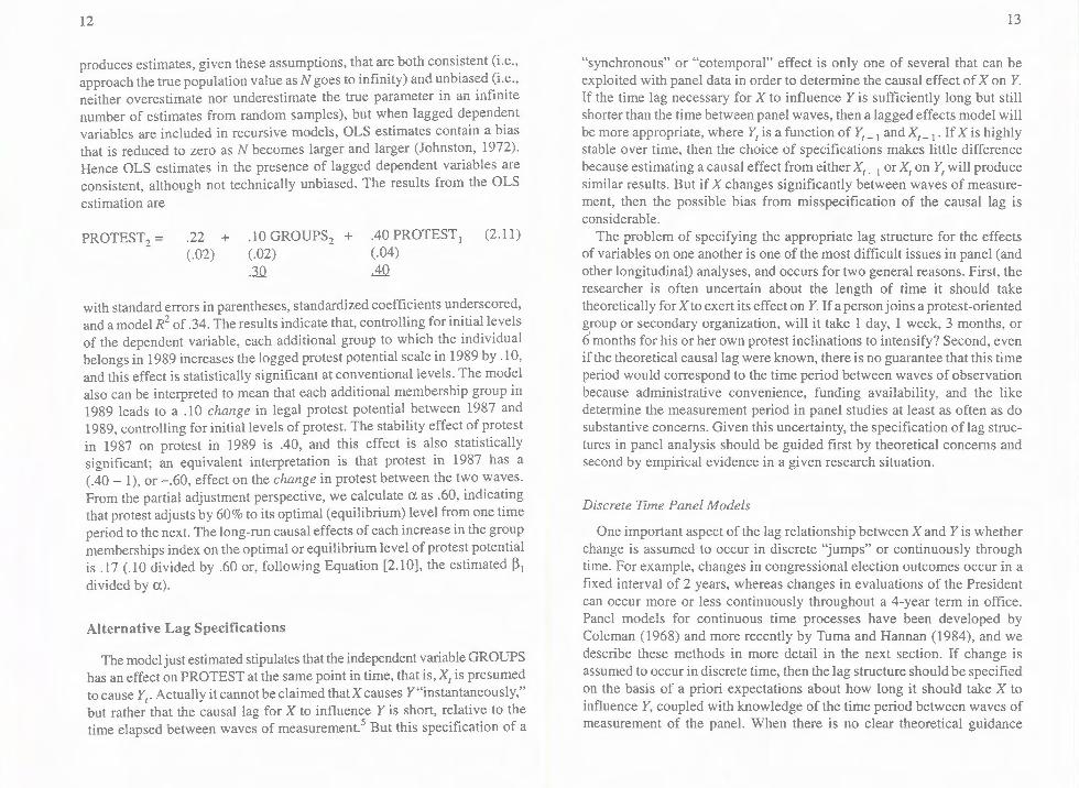
produces estimates, given these assumptions, that are both consistent (i.e.,approach the true population value as N goes to infinity) and unbiased (i.e.,neither overestimate nor underestimate the true parameter in an infinitenumber of estimates from random samples), but when lagged dependentvariables are included in recursive models, OLS estimates contain a biasthat is reduced to zero as N becomes larger and larger (Johnston, 1972).Hence OLS estimates in the presence of lagged dependent variables areconsistent, although not technically unbiased. The results from the OLSestimation are

PROTEST2 = .22 +(.02)

.10 GROUPS2 +(.02).30

.40 PROTEST 1

(.04)A:Q

(2.11)

13

"synchronous" or "cotemporal" effect is only one of several that can beexploited with panel data in order to determine the causal effect of X on Y.If the time lag necessary for X to influence Y is sufficiently long but stillshorter than the time between panel waves, then a lagged effects model willbe more appropriate, where YI is a function of YI_ 1 and X, _ 1• IfX is highlystable over time, then the choice of specifications makes little differencebecause estimating a causal effect from either X, _ 1 or X, on YIwill producesimilar results. But if X changes significantly between waves of measure­ment, then the possible bias from misspecification of the causal lag isconsiderable.The problem of specifying the appropriate lag structure for the effects

of variables on one another is one of the most difficult issues in panel (andother longitudinal) analyses, and occurs for two general reasons. First, theresearcher is often uncertain about the length of time it should taketheoretically forXto exert its effect on Y.Ifa person joins a protest-orientedgroup or secondary organization, will it take 1 day, 1 week, 3 months, or6'months for his or her own protest inclinations to intensify? Second, evenif the theoretical causal lag were known, there is no guarantee that this timeperiod would correspond to the time period between waves of observationbecause administrative convenience, funding availability, and the likedetermine the measurement period in panel studies at least as often as dosubstantive concerns. Given this uncertainty, the specification oflag struc­tures in panel analysis should be guided first by theoretical concerns andsecond by empirical evidence in a given research situation.

Discrete Time Panel Models

One important aspect of the lag relationship between Xand Y is whetherchange is assumed to occur in discrete "jumps" or continuously throughtime. For example, changes in congressional election outcomes occur in afixed interval of 2 years, whereas changes in evaluations of the Presidentcan occur more or less continuously throughout a 4-year term in office.Panel models for continuous time processes have been developed byColeman (1968) and more recently by Tuma and Hannan (1984), and wedescribe these methods in more detail in the next section. If change isassumed to occur in discrete time, then the lag structure should be specifiedon the basis of a priori expectations about how long it should take X toinfluence Y, coupled with knowledge of the time period between waves ofmeasurement of the panel. When there is no clear theoretical guidance

with standard errors in parentheses, standardized coefficients underscored,and amodel R2 of .34. The results indicate that, controlling for initial levelsof the dependent variable, each additional group to which the individualbelongs in 1989 increases the logged protest potential scale in 1989by .10,and this effect is statistically significant at conventional levels. The modelalso can be interpreted to mean that each additional membership group in1989 leads to a .10 change in legal protest potential between 1987 and1989, controlling for initial levels of protest. The stability effect of protestin 1987 on protest in 1989 is .40, and this effect is also statisticallysignificant; an equivalent interpretation is that protest in 1987 has a(.40 - 1), or -.60, effect on the change in protest between the two waves.From the partial adjustment perspective, we calculate a as .60, indicatingthat protest adjusts by 60% to its optimal (equilibrium) level from one timeperiod to the next. The long-run causal effects of each increase in the groupmemberships index on the optimal or equilibrium level of protest potentialis .17 (.10 divided by .60 or, following Equation [2.10], the estimated ~l

divided by a).

Alternative Lag Specifications

The modeljust estimatedstipulatesthat the independentvariableGROUPShas an effect on PROTEST at the same point in time, that is, X, is presumedto cause Yr Actually it cannot be claimed thatXcauses Y"instantaneously,"but rather that the causal lag for X to influence Y is short, relative to thetime elapsed between waves of measurement.' But this specification of a

14

regarding the appropriate lag length for model specification, then theanalyst may attempt to determine the causal lag empirically.

For example, we will analyze in later chapters the effect of an adoles­cent's involvement with a delinquent peer group on his or her own delin­quent behavior. In this case, a relatively short causal lag between X and Ymay be expected, as it would be unreasonable to expect an adolescent'speer group 2 or 3 years in the past to influence current behavior. Conse­quently, if panel data were gathered at 3-year intervals, a "lagged effect"model would not be the appropriate specification, and an "instantaneous"effect model might better capture the causal effect of delinquent peers onyouth delinquency. However, if the data were gathered at 1- or 2-monthintervals, this might coincide better with the actual time it would take forthe social pressure, planning, and so on in a peer group to result indelinquent behavior, and a lagged specification would be appropriate.Theoretical concerns might also dictate that a model include both lagged

and instantaneous effects. Consider the effect of stressful or traumatic lifeevents on an individual's psychological well-being. Given panel observa­tions of 1or 2 years, it may be expected that stressful life events influencepsychological health in the current period. At the same time, stressfulevents from 2 years previous to the current observation (X, _ I) may alsohave some lingering direct effects on current psychological health, or haveindirect influence on current well-being through unmeasured variablessuch as the individual's physical condition, job performance, and the like(Kessler & Greenberg, 1981, pp. 78-79).With unidirectional causal models, the inclusion of both X, and XI_ I in

the model poses no serious problems for estimation (aside from the possi­bility of high multicollinearity when the variable is extremely stable), andso a model of the following form can be estimated that may shed some lighton the appropriate lag relationship:

YI= Po+ PIXI+ P2YI-1 + P3XI_1 + EI· (2.12)

Such a formulation may also be amore intuitively appealing representationof the relationship between changes in both the independent and thedependent variables over time. The coefficients of this equation also canbe recast in terms of the changes in X by making use of the identityXI=XI_ I +AX. Thus Equation (2.12) can be expressed as

YI= Po+ P2 YI_I + (PI + P3)XI_1 + PI AX + EI· (2.13)

15

Note that PI' the effect of AX on YI in Equation (2.13), is the same as theeffect of XI on YI in (2.12); in other words, saying that the change in X hassome effect on YImeans that XIhas some effect on YI, controlling for X andY's prior values (Kessler & Greenberg, 1981, p. 10).The parameters of Equation (2.13) can be obtained through these alge­

braic manipulations or obtained directly (including their associated stan­dard errors) by including XI andAX as explanatory variables in a regressionmodel. Similar manipulations can be performed to transform Equation(2.12) into expressions for AX and X2 as well.6 Because the models arealgebraically equivalent, the substantive interpretation of the results willdepend on the theoretical assumptions of the model. In models of politicalstability, for example, it may be plausible to assume that instability is linkednegatively to a country's current economic level (X2) but affected posi­tively by changes in economic level over some period of time (AX), as thehypothesis of rapid economic growth as a "destabilizing force" suggests.Models of political campaign effects on voters might assume that anindividual's vote depended on some initial characteristics such as approvalof the incumbent administration's performance (XI) as well as changes inapproval (AX) that were induced by events or otherwise took place duringthe campaign (Finkel, 1993).Thus equations that include current and laggedvalues of X as predictors of the changes in Y can be interpreted in a varietyof ways depending on the substantive concerns of the model.We reestimate the static-score model from the group memberships­

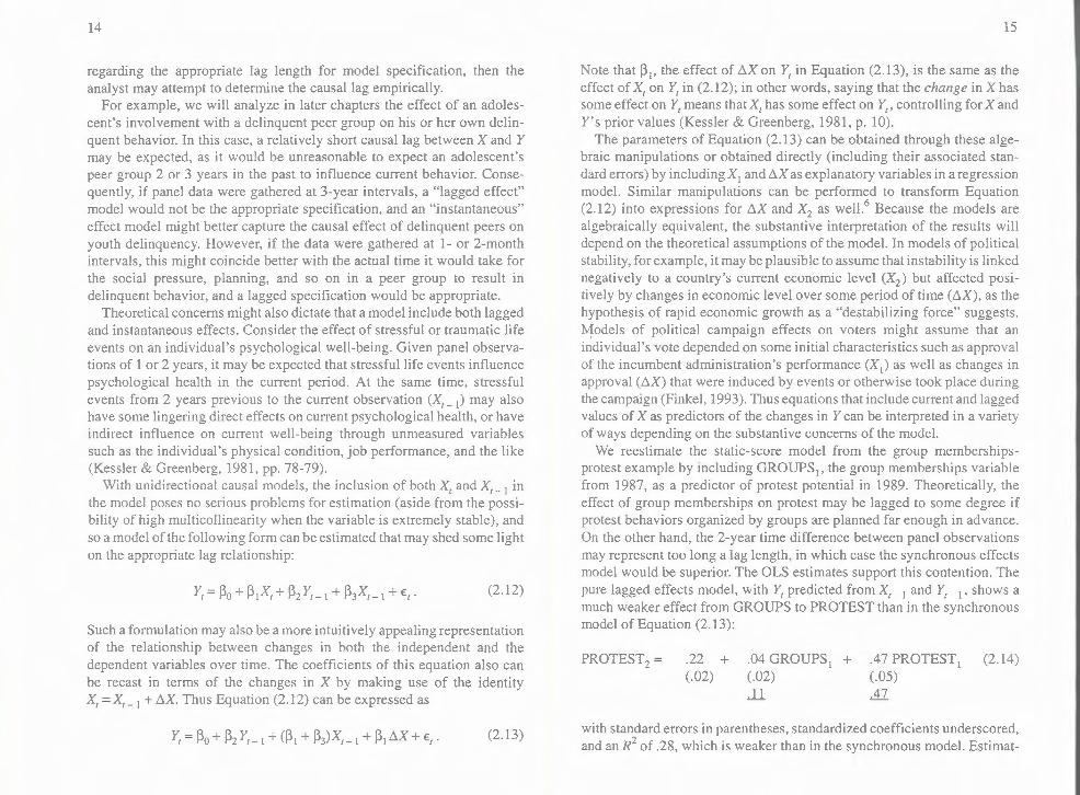
protest example by including GROUPSI' the group memberships variablefrom 1987, as a predictor of protest potential in 1989. Theoretically, theeffect of group memberships on protest may be lagged to some degree ifprotest behaviors organized by groups are planned far enough in advance.On the other hand, the 2-year time difference between panel observationsmay represent too long a lag length, in which case the synchronous effectsmodel would be superior. The OLS estimates support this contention. Thepure lagged effects model, with YI predicted from XI_ I and YI_ I' shows amuch weaker effect from GROUPS to PROTEST than in the synchronousmodel of Equation (2.13):

PROTEST2 = .22 +(.02)

.04 GROUPSI +(.02).u

.47 PROTEST I(.05).47

(2.14)

with standard errors in parentheses, standardized coefficients underscored,and an R2 of .28, which is weaker than in the synchronous model. Estimat-

16

ing a static-score model with both GROUPSI and GROUPS2 as inde­pendent variables yields the following results:

PROTEST2 =.22 + .11 GROUPS2(.02) (.02)

~

(2.15)+ .40 PROTEST I

(.04)All

+ -.01 GROUPS I(-.02)-.02

with standard errors in parentheses, standardized coefficients underscored,and anR2 value of .34. The results indicate that current group membershipsis significantly related to protest potential, controlling for lagged Y andlagged group memberships. Controlling for current group memberships,lagged group memberships is statistically insignificant and adds littleadditional explanatory power to the model. Following Equation (2.13), theeffect of GROUPS2 also may be interpreted as the effect of the changes ingroup memberships on PROTEST2' controlling for lagged group member-ships and lagged protest potential.

Panel Models in Continuous TimeThe previous section discussed procedures for estimating the proper lag

structure for the effects of X to be felt on Yover a given time interval. Ifthe theoretical lag length matched the length of time between waves ofobservation, a lagged effects model would be preferred, whereas if the laglength was much shorter than the length between waves, a synchronouseffects model would be superior. In some panel models, however, theinfluence of X on Y can be viewed as occurring more or less continuouslythrough time, rather than in a discrete jump between the waves of obser­vation of the panel. For example, the effect of individuals' party affiliationson their attitudes about presidential candidates might operate continuouslythroughout a campaign, as individuals may constantly adjust their ratingsof the major party candidates in response to their underlying party loyaltiesas time progressed. Organizations might adjust their employment basemore or less continuously in response to economic forces in the environ­ment. Such models have much intuitive and theoretical appeal for analyz­ing many of the dependent variables typically studied by social scientists,such as attitudes and other social-psychological constructs, organizationalchange, and population movements. In these cases, measurements taken atparticular times in a given panel study represent purely arbitrary timeintervals for the observations of the causal process to have been made, and

,,-

17

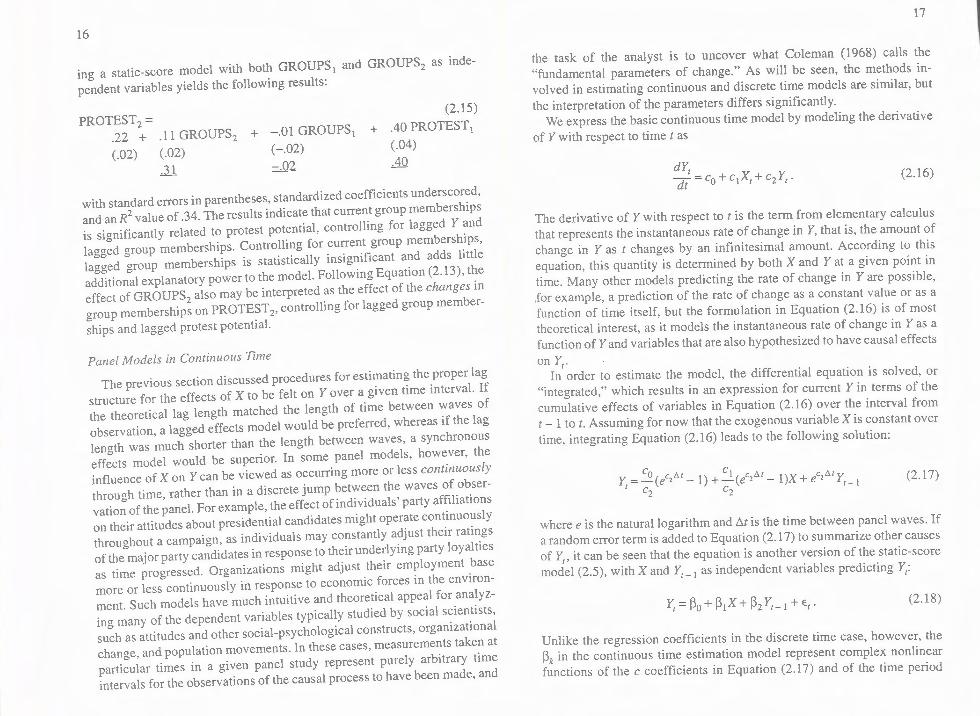
the task of the analyst is to uncover what Coleman (1968) calls the"fundamental parameters of change." As will be seen, the methods in­volved in estimating continuous and discrete time models are similar, butthe interpretation of the parameters differs significantly.We express the basic continuous time model by modeling the derivative

of Y with respect to time t as

dYIdt = Co+ c IXI + c2 YI • (2.16)

The derivative of Y with respect to t is the term from elementary calculusthat represents the instantaneous rate of change in Y, that is, the amount ofchange in Y as t changes by an infinitesimal amount. According to thisequation, this quantity is determined by both X and Yat a given point intime. Many other models predicting the rate of change in Yare possible,for example, a prediction of the rate of change as a constant value or as afunction of time itself, but the formulation in Equation (2.16) is of mosttheoretical interest, as it models the instantaneous rate of change in Yas afunction of Yand variables that are also hypothesized to have causal effectson YI•In order to estimate the model, the differential equation is solved, or

"integrated," which results in an expression for current Y in terms of thecumulative effects of variables in Equation (2.16) over the interval fromt - 1 to t.Assuming for now that the exogenous variable X is constant overtime, integrating Equation (2.16) leads to the following solution:

c cY =~(eC2M _ 1)+.....!.(eC2M - l)X + eC2t.lyI c2 c2 I-I

(2.17)

where e is the natural logarithm and /).t is the time between panel waves. Ifa random error term is added to Equation (2.17) to summarize other causesof YI, it can be seen that the equation is another version of the static-scoremodel (2.5), with X and Yt-I as independent variables predicting YI:

Yt=~O+~IX+~2Yt-1 +Et•(2.18)

Unlike the regression coefficients in the discrete time case, however, the~k in the continuous time estimation model represent complex nonlinearfunctions of the c coefficients in Equation (2.17) and of the time period

18

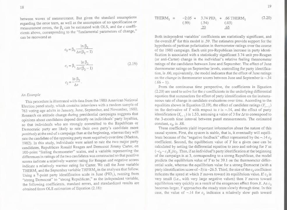
between waves of measurement. But given the standard assumptionsregarding the error term, as well as the assumption of no specification ormeasurement errors, the ~k can be estimated with OLS, and the c coeffi­cients above, corresponding to the "fundamental parameters of change,"can be recovered as

In ~2

Co= ~o ~t(~2 - 1)

In ~2 (2.19)c} =~}~t(~2 - 1)

In ~2

<:«:An Example

This procedure is illustrated with data from the 1980American NationalElection panel study, which contains interviews with a random sample of763 voting-age adults in January, June, September, and November, 1980.Research on attitude change during presidential campaigns suggests thatopinions about candidates depend directly on individuals' party loyalties,so that individuals who are strongly committed to the Republican orDemocratic party are likely to rate their own party's candidate morepositively at the end of a campaign than at the beginning, whereas they willrate the candidate of the opposing party more negatively over time (Markus,1982). In this study, individuals were asked to rate the two major partycandidates, Republican Ronald Reagan and Democrat Jimmy Carter, on100-point "feeling thermometer" scales, and a variable representing thedifferences in ratings of the two candidates was constructed so that positivescores indicate a relatively warmer rating for Reagan and negative scoresindicate a relatively warmer rating for Carter. We call the June variableTHERM}and the September variable THERM2in the analyses that follow.Using a 7-point party identification scale in June (PID}), running from"strong Democrat" to "strong Republican," as the independent variable,the following coefficients, standard errors, and standardized results areobtained from OLS estimation of Equation (2.18):

THERMz (2.20)

19

-2.0S +(.99)

3.74 PID} +(.S4).20

.66THERM}(.03).&5.

Both independent variables' coefficients are statistically significant, andthe overall R2 for this model is .S9. The estimates provide support for thehypothesis of partisan polarization in thermometer ratings over the courseof the 1980 campaign. Each unit pro-Republican increase in party identi­fication is associated with a statistically significant 3.74 unit pro-Reagan(or anti-Carter) change in the individual's relative feeling thermometerratings of the candidates between June and September. The effect of Junethermometer ratings on September levels, controlling for party identifica­tion, is .66; equivalently, the model indicates that the effect of June ratingson the change in thermometer scores between June and September is -.34(.66 - 1)., From the continuous time perspective, the coefficients in Equation(2.20) are used to solve for the c coefficients in the underlying differentialequation that summarizes the effect of party identification on the instanta­neous rate of change in candidate evaluations over time. According to theequalities shown in Equation (2.19), the effect of candidate ratings (Yt-})

on the derivative of Y with respect to t is -.14, and the effect of partyidentification (Xt_}) is 1.S3, assuming a value of 3 for ~t to correspond tothe 3-month time interval between panel measurements. The estimatedconstant, co' is .88.These coefficients yield important information about the nature of this

causal system. First, the system is stable, that is, it eventually will equili­brate because of the "negative feedback" effect represented by the -.14 Czcoefficient. Second, the equilibrium value of Y for a given case can becalculated by setting the differential equation to zero and solving for Yas(-co - c}X})!c2· Thus, if an individual's party identification at the beginningof the campaign is at 3, corresponding to a strong Republican, the modelpredicts the equilibrium value of Y to be 39.1 on the thermometer differ­ential scale, whereas the equilibrium value for a strong Democrat (with aparty identification score of -3) is -26.S. Third, the size of the c2coefficientindicates the speed at which Y moves toward its equilibrium value. If c2 isvery small (i.e., with very large negative values) then Y moves towardequilibrium very quickly as a result of the exogenous effect from X. As Czbecomes larger, Yapproaches the steady state slowly through time. In thiscase, the value of -.14 for c2 indicates a relatively slow path toward

20

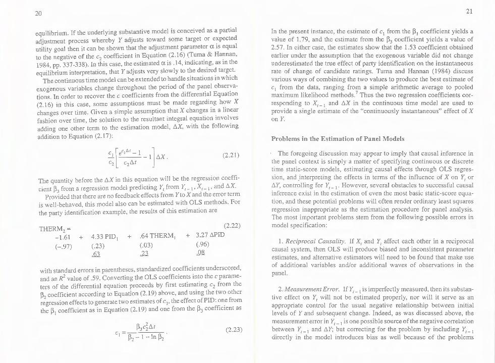
equilibrium. If the underlying substantive model is conceived as a partialadjustment process whereby Y adjusts toward some target or expectedutility goal then it can be shown that the adjustment parameter a. is equalto the negative of the c2 coefficient in Equation (2.16) (Tuma & Hannan,1984,pp. 337-338). In this case, the estimated a. is .14, indicating, as in theequilibrium interpretation, that Y adjusts very slowly to the desired target.The continuous time model can be extended to handle situations in which

exogenous variables change throughout the period of the panel observa­tions. In order to recover the c coefficients from the differential Equation(2.16) in this case, some assumptions must be made regarding how Xchanges over time. Given a simple assumption that X changes in a linearfashion over time, the solution to the resultant integral equation involvesadding one other term to the estimation model, I1X, with the followingaddition to Equation (2.17):

s.[eC2{1,t - 1 ]c2 c211t - 1 I1X. (2.21)

The quantity before the I1X in this equation will be the regression coeffi­cient P3 from a regression model predicting Yt from Yt- 1' Xt_ i-and 11X.Provided that there are no feedback effects from Y toX and the error term

is well-behaved, this model also can be estimated with OLS methods. Forthe party identification example, the results of this estimation are

THERM2=-1.61 +(-.97)

(2.22)+ 3.27!1PID

(.96)_,QB.

4.33 PID1(.23).63

+ .64THERM1(.03).,2.3.

with standard errors in parentheses, standardized coefficients underscored,and an R2 value of .59. Converting the OLS coefficients into the c parame­ters of the differential equation proceeds by first estimating c2 from theP2coefficient according to Equation (2.19) above, and using the two otherregression effects to generate two estimates of ci- the effect ofPID: one fromthe P1coefficient as in Equation (2.19) and one from the P3 coefficient as

P3C;!1t (2.23)c1 = P2 - 1 -l~ P2

In the present instance, the estimate of cI from the PI coefficient yields avalue of 1.79, and the estimate from the P3 coefficient yields a value of2.57. In either case, the estimates show that the 1.53 coefficient obtainedearlier under the assumption that the exogenous variable did not changeunderestimated the true effect of party identification on the instantaneousrate of change of candidate ratings. Tuma and Hannan (1984) discussvarious ways of combining the two values to produce the best estimate ofcI from the data, ranging from a simple arithmetic average to pooledmaximum likelihood methods.I Thus the two regression coefficients cor­responding to Xt_ I and I1X in the continuous time model are used toprovide a single estimate of the "continuously instantaneous" effect of Xon Y.

Problems in the Estimation of Panel Models

The foregoing discussion may appear to imply that causal inference inthe panel context is simply a matter of specifying continuous or discretetime static-score models, estimating causal effects through OLS regres­sion, and .interpreting the effects in terms of the influence of X on Yt orI1Y, controlling for Yt-1. However, several obstacles to successful causalinference exist in the estimation of even the most basic static-score equa­tion, and these potential problems will often render ordinary least squaresregression inappropriate as the estimation procedure for panel analysis.The most important problems stem from the following possible errors inmodel specification:

1. Reciprocal Causality. IfX, and Yt affect each other in a reciprocalcausal system, then OLS will produce biased and inconsistent parameterestimates, and alternative estimators will need to be found that make useof additional variables and/or additional waves of observations in thepanel.

2.Measurement Error. IfYt- Iis imperfectly measured, then its substan­tive effect on Yt will not be estimated properly, nor will it serve as anappropriate control for the usual negative relationship between initiallevels of Y and subsequent change. Indeed, as was discussed above, themeasurement error in Yt- Iis one possible source of the negative correlationbetween Yt-1 and I1Y; but correcting for the problem by including Yt-1

directly in the model introduces bias as well because of the problems

21

22

associated with statistical estimation in the presence of error-laden inde­pendent variables. This bias often leads to the underestimation of the trueeffect of Yt-1 on Yt, and to the overestimation of the estimated effects ofthe other explanatory variables.

3. Omitted Variablesand Autocorrelated Disturbances. Finally, omittedvariables can lead to several kinds of biases in panel models. Aside fromthe usual specification bias that may result from an omitted variable'scorrelation with observed independent variables, omitted variables in panelmodels may lead to autocorrelation in the endogenous variable's errorterms over time. This in tum produces a nonzero correlation betweenYt-1 and Et, yielding inconsistent OLS estimates of the effects of Yt-1 onYt in the static-score model. If the other independent variables are relatedto Yt- l' autocorrelated disturbances may bias the estimates of their effectson Yt as well.

These issues in the specification and estimation of static-score panelmodels will occupy the discussion for the remainder of the monograph.Although all of these problems present serious obstacles to successfulcausal inference, it will be seen that panel data often provide enoughinformation to estimate parameters successfully in the face of these diffi­culties. In addition, many of these problems are endemic in all empiricalresearch, and it will be shown that panel data provide the researcher withfar greater ability to control these problems than is attained in cross­sectional analyses.

3. MODELS OF RECIPROCAL CAUSATION

The models in the previous chapter all contained the assumption that therelationship between X and Y was unidirectional, that is, that X influencedY but not the reverse. In some instances, this assumption is entirelyappropriate. For example, in models of the effects of race or other ascribedcharacteristics on an individual's income over time, or in research thatmodels the effects of early adult experiences on later political or socialorientations, the temporal (and hence potential causal) ordering betweenvariables is clear. In other cases, theoretical reasons might preclude thetesting of reciprocal causation, as, for example, in research that attemptsto model the effects of economic indicators on government popularity in aset of countries observed over time. In these models, Xt' Xt-1, and/or ll.X

can be treated as exogenous variables in their respective equations, andparameter estimates can be obtained through OLS regression or, if theassumptions of no measurement error or autocorrelated disturbances can­not be justified, through procedures that will be discussed in later chapters.But in many analyses, the assumption of unidirectional causality is not

tenable, and indeed one of the primary motivations for analyzing panel datais to attempt to determine the causal ordering between the variables ofinterest. For example, we hypothesized in the previous chapter that groupmemberships influence an individual's behavioral orientation to protest,and that individuals' long-standing party attachments determine their feel­ings about presidential candidates during an election campaign; but theo­ries of participation and group mobilization suggest that participation inprotest activities may lead individuals to join more groups with a protestorientation, and theories of political partisanship suggest that attitudesabout political candidates might alter individuals' long-term party loyalties,aswell. In these cases, theoretical concerns lead to plausible expectationsof reciprocal causal relationships between X and Y.Panel data-offer decided advantages over cross-sectional analyses in

testing for potential reciprocal causal effects between variables. Becausecross-sectional data are collected at a single point in time, reciprocal effectsmodels can be specified only with synchronous, or simultaneous, causalinfluences from one variable to the other, and the estimation of reciprocalcausal effects would proceed by incorporating outside variables in an"instrumental variables" or Two Stage Least Squares analysis (Berry,1984). However, the success of these methods depends, as we will seebelow, on the model satisfying several restrictive assumptions about therelationship of these outside variables with X, Y, and the disturbance termsof their respective equations. As shown in Chapter 2, the temporal compo­nent of panel designs allows the researcher to estimate models with laggedcausal effects, where prior values of X influence future values of Y (or thechange in Y), and vice versa. Further, models with reciprocal simultaneousor synchronous causal effects may be identified and estimated under certainconditions without making the possibly dubious assumptions about theeffectsof outside instrumental variables that are necessary in cross-sectionalresearch.This chapter outlines the uses of panel data in assisting in causal

inference in models with reciprocal effects between variables. It will beemphasized that panel designs are a powerful means of estimating recip­rocal causal effects, although they offer no automatic method for "provingcausality." The estimation of reciprocal effects always takes place within

23