Capco Institute - HESGE

The Capco Institute

Journal of Financial Transformation #30 11.2010

JournalThe Capco Institute Journal of Financial Transformation

#30Industrialization of Finance

11.2010

Recipient of the Apex Awards for Publication Excellence 2002-2010

CapCo.Com

amsterdamantwerp

BangaloreChicago

FrankfurtGenevaLondon

New Yorkparis

San FranciscoToronto

Washington, D.C.Zurich

MSc in Insurance and Risk Management

Cass is one of the world’s leading academic centresin the insurance field. What's more, graduatesfrom the MSc in Insurance and Risk Managementgain exemption from approximately 70% of theexaminations required to achieve the AdvancedDiploma of the Chartered Insurance Institute (ACII).

For applicants to the Insurance and RiskManagement MSc who already hold a CII Advanced Diploma, there is a fast-track January start, giving exemption from the first term of the degree.

To find out more about our regular informationsessions, the next is 10 April 2008, visitwww.cass.city.ac.uk/masters and click on'sessions at Cass' or 'International & UK'.

Alternatively call admissions on:

+44 (0)20 7040 8611

With a Masters degree from Cass Business School,you will gain the knowledge and skills to stand out in the real world.

Minimise risk,optimise success

JournalEditorShahin Shojai, Global Head of Strategic Research, Capco

Advisory EditorsCornel Bender, Partner, CapcoChristopher Hamilton, Partner, CapcoNick Jackson, Partner, Capco

Editorial BoardFranklin Allen, Nippon Life Professor of Finance, The Wharton School, University of PennsylvaniaJoe Anastasio, Partner, CapcoPhilippe d’Arvisenet, Group Chief Economist, BNP ParibasRudi Bogni, former Chief Executive Officer, UBS Private BankingBruno Bonati, Strategic Consultant, Bruno Bonati ConsultingDavid Clark, NED on the board of financial institutions and a former senior advisor to the FSAGéry Daeninck, former CEO, RobecoStephen C. Daffron, Global Head, Operations, Institutional Trading & Investment Banking, Morgan StanleyDouglas W. Diamond, Merton H. Miller Distinguished Service Professor of Finance, Graduate School of Business, University of ChicagoElroy Dimson, BGI Professor of Investment Management, London Business SchoolNicholas Economides, Professor of Economics, Leonard N. Stern School of Business, New York UniversityMichael Enthoven, Former Chief Executive Officer, NIBC Bank N.V. José Luis Escrivá, Group Chief Economist, Grupo BBVAGeorge Feiger, Executive Vice President and Head of Wealth Management, Zions BancorporationGregorio de Felice, Group Chief Economist, Banca IntesaHans Geiger, Professor of Banking, Swiss Banking Institute, University of ZurichPeter Gomber, Full Professor, Chair of e-Finance, Goethe University FrankfurtWilfried Hauck, Chief Executive Officer, Allianz Dresdner Asset Management International GmbHPierre Hillion, de Picciotto Chaired Professor of Alternative Investments and Shell Professor of Finance, INSEADThomas Kloet, Chief Executive Officer, TMX Group Inc.Mitchel Lenson, former Group Head of IT and Operations, Deutsche Bank GroupDonald A. Marchand, Professor of Strategy and Information Management, IMD and Chairman and President of enterpriseIQ®

Colin Mayer, Peter Moores Dean, Saïd Business School, Oxford University John Owen, Chief Operating Officer, Matrix GroupSteve Perry, Executive Vice President, Visa EuropeDerek Sach, Managing Director, Specialized Lending Services, The Royal Bank of ScotlandManMohan S. Sodhi, Professor in Operations & Supply Chain Management, Cass Business School, City University LondonCharles S. Tapiero, Topfer Chair Distinguished Professor of Financial Engineering and Technology Management, New York University Polytechnic InstituteJohn Taysom, Founder & Joint CEO, The Reuters Greenhouse FundGraham Vickery, Head of Information Economy Unit, OECDNorbert Walter, Managing Director, Walter & Daughters Consult

Part 19 A Critique of Alan Greenspan’s Retrospective

on the CrisisJerome L. Stein

23 Share Price Disparity in Chinese Stock MarketsTom Fong, Alfred Wong, Ivy Yong

33 How Might Cell Phone Money Change the Financial System?Shann Turnbull

43 Technology Simplification and the Industrialization of Investment BankingSimon Strong

49 Compliance Function in Banks, Investment and Insurance Companies after MiFIDPaola Musile Tanzi, Giampaolo Gabbi, Daniele Previati, Paola Schwizer

57 Investor Irrationality and Closed-end Hedge FundsOliver Dietiker

67 Next Generation Niche MarketsAllan D. Grody, Peter J. Hughes

73 Global Financial Centers – Growth and Competition after the CrisisSteffen Kern

83 Unwrapping Fund Expenses: What are You Paying For?Brian J. Jacobsen

89 Securitization of Financial Asset/Liability Products with Longevity RiskCarlos E. Ortiz, Charles A. Stone, Anne Zissu

Part 295 Preventing the Next Great Meltdown

David A. Levine

105 Enhancing the Transparency of Bank Fair Value ReportingPaul Klumpes, Peter Welch

121 Constraints to Improving Financial Sector RegulationDan Ciuriak

127 The IFC’s New Africa, Latin America, and Caribbean Fund: Its Worrisome Start, and How to Fix ItPatrick J. Keenan, Christiana Ochoa

133 Regulation Effects on Stock Returns in Shanghai and Shenzhen ExchangesHaim Kedar-Levy, Xiaoyan Yu, Akiko Kamesaka, Uri Ben-Zion

141 Operational Risk Management Using a Fuzzy Logic Inference SystemAlejandro Reveiz, Carlos León

155 Bringing Islamic Banking into the Mainstream is Not an Alternative to Conventional Finance Ewa Karwowski

163 A Case Against Speculation by Deposit Taking BanksKosrow Dehnad

169 The Emergent Evolution of Human Risks in Service Companies Due to Control Industrialization: An Empirical ResearchEmmanuel Fragnière, Nathalie Junod

Industrialization of Finance

Welcome to the latest edition of our

Journal. Why “the industrialization of

finance”?

Because post-crisis, as we re-build an

industry that is ready for the opportuni-

ties of the future, we need to focus on the

strategies and implementation that will

help us all work more reponsively, more

efficiently, and in ways that shape the

future of financial services positively and

sustainably.

By “industrializing” what we do, we are

not advocating a mechanical or unimagi-

native approach – quite the opposite.

What we are saying is that techniques

and tools exist to make the commod-

itized and process aspects of the indus-

try as reliable, predictable and efficient as

possible, while focusing on what will dif-

ferentiate customer service and product

innovation.

At Capco, we have no doubt of the will

and the creativity that already exist within

global financial services. These qualities

are ready to be applied to the tasks of

meeting stakeholder expectations and

rising to the challenges of transforma-

tional change. Yes, the lessons of recent

history are still poignant. But intense com-

petition, reduced margins and the need

to identify and exploit new markets are

evident in every industry. The automotive,

retail, pharmaceutical, and in truth every

industrial and commercial sector can

tell a similar story of enormous change.

The greatest difference perhaps is that

our sector sits at the heart of national,

regional and global economic recovery

and prosperity. The expectations and the

pressures are therefore even greater. And

our responses have to be all the more

robust.

Of course, we need to temper optimism

with realism: blind faith is not a sound

basis for the years ahead. But we also

need to bear in mind that by its very

nature, history happens in the rearview

mirror. Our task now is to look forward.

Ahead lie some serious responsibilities,

not least to comply with a rapidly evolv-

ing regulatory framework, while rising to

the expectations of a far broader range of

stakeholders (who now include in many

cases national governments and their

electorates, as well as traditional share-

holders).

So the future will be different. And that

means our responses, not least in terms

of operational efficiencies and improved

technology platforms, will need to be

positively different as well. Yet this is

absolutely not beyond the scope of our

collective imagination, expertise and tal-

ent. By tackling complexity and exploiting

the amazing march of connectivity, we

can do traditional things in new and bet-

ter ways, and we can offer our stakehold-

ers more of what they want and need.

As this latest edition of the Journal illus-

trates, some keen intellects are focused

on the challenges that face us. As we

“industrialize” we also have an opportu-

nity to build a financial services sector

that is the polar opposite of the negative

assertions we have all heard since the

most recent crisis. I hope you enjoy the

views and insights of our Journal con-

tributors. Incidentally, this edition reflects

our faith in the renaissance of the industry

by carrying the look and feel of our new

branding – which I hope will meet with

your approval.

As ever, we look forward to your feed-

back and to playing our part at Capco in

forming the future of finance.

With warm good wishes,

Rob Heyvaert,

Founder and CEO, Capco

Dear Reader,

The world of finance has undergone a

renaissance in recent years. Many of

the long held beliefs about the subject

have been shattered. Pricing models

that used to be viewed as the cor-

nerstone of finance have come under

tremendous scrutiny by those who do

not have a vested interest in protect-

ing their lifetime of research. While

many academics are clinging onto the

notion of efficient markets, the real

world has moved on and is looking

for more reliable ways in which assets

can be priced. Risk measurement and

management models that were viewed

as airtight even as recently as a couple

of years ago have been proven to be

anything but.

The implication of the failure of aca-

demic, and to a large extent applied,

finance has been that many have

started to look for new ways in which

stakeholders can be protected and

even develop new ways in which finan-

cial institutions should model risk and

asset pricing. This is essential if we are

to avoid the same kind of hubris-based

crises in the future. But, of course,

finance is more than just reliable asset

and risk pricing. Our industry is begin-

ning to understand that it too needs to

learn how an industry and its constitu-

ent companies should best be man-

aged.

It is at the point at which previous fail-

ures are objectively questioned and

new models developed that an industry

comes of age, and finance is certainly

doing that. It is at last joining its peers

in other industries in learning to ask the

tough questions and ignore the attacks

of those members of the academia

who have a vested interest in maintain-

ing the status quo. We are at a similar

point that physics was when gravity

was identified, or when it was proven

that the world is round. The entire

premise of the subject has changed

and significantly more innovative, and

more importantly practical models, will

certainly be developed. They are nec-

essary since like all other industries

that came before us we are learning

to operate in a complex world in which

competition will result in the erosion of

margins, where reliable pricing is key,

and where innovation is essential for

success.

It is due to the fact that we are witness-

ing the industrialization of finance that

we have dedicated this edition of the

Journal to this subject. The papers in

this issue examine the impact of the

anticipated changes in the regulatory,

technological, and competitive environ-

ment on the financial services industry

and try and provide prescriptive solu-

tions to how they can be most effec-

tively met. The topics covered range

from looking at how old instruments

and markets are changing, to the impli-

cations of helping the future generation

of bankers in developing economies. In

reality, this is the first edition of a long

series of issues dedicated to the topic

of industrialization of finance.

We hope that you enjoy the articles in

this edition of the Journal and that you

continue to support us by submitting

your ideas to us.

On behalf of the board of editors

Finance is Coming of Age

Part 1A Critique of Alan Greenspan’s Retrospective on the Crisis

Share Price Disparity in Chinese Stock Markets

How Might Cell Phone Money Change the Financial System?

Technology Simplification and the Industrialization of Investment Banking

Compliance Function in Banks, Investment and Insurance Companies after MiFID

Investor Irrationality and Closed-end Hedge Funds

Next Generation Niche Markets

Global Financial Centers – Growth and Competition after the Crisis

Unwrapping Fund Expenses: What are You Paying For?

Securitization of Financial Asset/Liability Products with Longevity Risk

9

PART 1

A Critique of Alan Greenspan’s Retrospective on the Crisis

AbstractAlan Greenspan’s paper (March 2010) presents his retro-

spective view of the crisis. His theme has several parts. First,

the housing price bubble, its subsequent collapse, and the

financial crisis were not predicted either by the market, the

Fed, the IMF, or the regulators in the years leading to the cur-

rent crisis. Second, financial intermediation tried to function

on too thin layer of capital – high leverage – owing to a mis-

reading of the degree of risk embodied in ever more complex

financial products and markets. Third, the breakdown was

unpredictable and inevitable, given the “excessive” leverage

– or low capital – of the financial intermediaries. Greenspan

now focuses on desirable capital requirements for banks

and financial intermediaries. Too high a capital requirement

will not provide a sufficiently high rate of return on finan-

cial assets to attract capital. Too low a capital requirement

unduly raises risk and endangers bank solvency. The Fed,

IMF, the Treasury, and the market lacked the appropriate

tools of analysis to answer the following questions: what

is an optimal leverage or capital requirement that balances

the expected growth against risk? What are theoretically

founded early warning signals of a crisis? I explain why the

application of stochastic optimal control (SOC)/dynamic risk

management is an effective approach to determine the op-

timal degree of leverage, the optimum and excessive risk,

and the probability of a debt crisis. The theoretically derived

early warning signal of a crisis is the excess debt ratio, equal

to the difference between the actual and optimal ratio. The

excess debt starting from 2004-05 indicated that a crisis

was most likely. This SOC analysis should be used by those

charged with surveillance of financial markets.

Jerome L. Stein — Division of Applied Mathematics, Brown University

10

Greenspan’s themePrior to the subprime crisis of 2007, there was a false sense of safety

in financial markets. Alan Greenspan (2004a) said that “…the surge in

mortgage refinancings likely improved rather than worsened the financial

condition of the average homeowner.” Moreover “[o]verall, the household

sector seems to be in good shape, and much of the apparent increase in

the household sector’s debt ratios in the past decade reflects factors that

do not suggest increasing household financial stress.”

The market and the Fed did not consider these mortgages to be very

risky. In February 2004, a few months before the Fed formally ended a

run of interest rate cuts, Greenspan (2004b) said that “…improvements

in lending practices driven by information technology have enabled lend-

ers to reach out to households with previously unrecognized borrowing

capacity. This extension of lending has increased overall household debt

but has probably not meaningfully increased the number of households

with already overextended debt.” By 2007, a measure of risk, the yield

spread (CCC bonds – 10 year U.S. Treasury) fell to a record low. Ben

Bernanke (2005) said in his testimony before Congress’s Joint Economic

Committee that U.S. house prices had risen by nearly 25 percent over the

past two years. However, these increases “largely reflect strong econom-

ic fundamentals” such as strong growth in jobs, incomes and the number

of new households. The failure to realize that there was an unsustainable

bubble that would damage the world economy was pervasive. As late as

April 2007, the IMF noted that “…global economic risks declined since

… September 2006 … The overall U.S. economy is holding up well …

[and] the signs elsewhere are very encouraging.” The venerated credit

rating agencies bestowed credit ratings that implied Aaa smooth sailing

for many a highly toxic derivative product.

In 2008 Greenspan said, “Those of us who have looked to the self-interest

of lending institutions to protect stockholders’ equity, myself included, are

in a state of disbelief.” In his retrospective he asks: could the breakdown

have been prevented? The Fed was lulled into complacency about a burst-

ing of the bubble and its aftermath because of recent history. First, they an-

ticipated that the decline in home prices would be gradual. Second, there

were only modestly negative effects of the 1987 stock market crash. The

injections of Fed liquidity apparently helped to stabilize the economy.

Greenspan’s paper (2010) presents his retrospective view of the crisis. His

theme has several parts. First, the decline and convergence of world real

long term interest rates – not Federal Reserve monetary policy – led to

significant housing price appreciation, a housing price bubble. This bub-

ble was leveraged by debt. There was a heavy securitization of subprime

mortgages. In the years leading to the current crisis, financial intermedia-

tion tried to function on too thin layer of capital – high leverage – owing

to a misreading of the degree of risk embodied in ever more complex

financial products and markets. Second, when the bubble unraveled, the

leveraging set off a series of defaults. Third, the breakdown of the bubble

was unpredictable and inevitable, given the “excessive” leverage – or

unduly low capital – of the financial intermediaries. Fourth, the lesson for

the future is that it is imperative that there be an increase in regulatory

capital and liquidity requirements by banks.

The theme of my paper has several interrelated parts. First, the failure

to anticipate the bubble, its collapse, and effect upon the economy

stemmed from the absence of a theoretical model, with explanatory pow-

er, that measures what is an “excessive” debt or leverage or unduly low

capital requirement that will raise the probability of a crisis. Such a model

must take into account that the future movements of key variables are

stochastic, and that the optimal leverage optimally balances expected

return against risk. Second, Greenspan’s (2010) suggestion of a minimum

capital requirement is indeed a move in the correct direction, but could

benefit from theoretical foundations. Third and foremost, the appropriate

technique for the analysis is stochastic optimal control (SOC). On the

basis of the SOC analysis, I derive a theoretically founded “early warning

signal” (EWS). This EWS is the “excessive” debt, equal to the difference

between the actual and optimal debt ratio, which would have predicted

the crisis. Moreover, the optimal debt ratio implies the optimal capital

requirement that Greenspan is seeking. Greenspan and Bernanke would

have benefitted had their staff had the analytic tool developed here. It is

hoped that the Fed will not be like the ancien régime: “Ils n’ont rien ap-

pris, ni rien oublié.”

The Jackson Hole ConsensusOtmar Issing (2010) discussed the lessons to be learned by central banks

from the recent financial crisis. The main thrust of his argument was a

criticism of the Jackson Hole Consensus [JHC (2005)] for the relation

between asset price bubbles and the conduct of monetary policy.

During the boom years, abundant liquidity and low interest rates led to a

situation of excessive risk taking and asset price bubbles. The JHC has

been the prevailing regulatory approach taken by the Fed. It is based

upon three principles. Central banks: (1) should not target asset prices,

(2) should not try to prick an asset price bubble, (3) should follow a “mop-

ping up” strategy after the bubble bursts by injecting enough liquidity to

avoid serious effects upon the real economy. A justification for this policy

was seen in the period 2000-02 with the collapse of the dot.com bubble.

The “mopping up” seemed to work well and there were no serious ef-

fects upon the real economy from following the JHC. Issing objects to the

JHC because it constitutes an asymmetric approach. When asset prices

rise without inflationary effects measured by the CPI, this is deemed ir-

relevant for monetary policy. But when the bubble bursts, central banks

must come to the rescue. This, he argues, produces a moral hazard. He

notes that although the JHC strategy worked well in the 2000-02 period

it should not have justified the assumption that it would work afterwards

11

in other cases. The JHC strategy certainly did not work in the 2007-08

crisis that was precipitated by the bursting of the housing price bubble.

He wrote: “Did we really need a crisis that brought the world to the brink

of a financial meltdown to learn that the philosophy which was at the time

seen as state of the art was in fact dangerously flawed? ...We must con-

duct a thorough discussion as to appropriate strategy of central banks

with respect to asset prices.”

Issing favors giving the central banks a mandate for macro-prudential

supervision, the proposal by the Larosière group. The ECB should be

responsible for identifying macroeconomic imbalances and for issuing

warnings and recommendations addressed to national policymakers.

The “solution” proposed is one that monitors closely monetary and credit

developments as the potential driving forces for consumer price inflation

in the medium to short run. “As long as money and credit remain broadly

controlled, the scope for financing unsustainable runs in asset prices

should also remain limited.” He notes: “numerous empirical studies have

shown that almost all asset price bubbles have been accompanied, if

not preceded by strong growth of credit and or money.” However, these

studies, such as reported by the BIS [Borrio and Lowe (2002)], are vague

and inconclusive. Even their authors conclude that the existing literature

provides little insight into the key question that is of concern to central

banks and supervisory authorities: when should credit growth be judged

“too fast”? Moreover, contrary to Issing, it is very difficult to find a rela-

tion between recent money growth and the 2007-08 financial crisis. The

BIS makes suggestions for further research. (1) Such work should pay

greater attention to conceptual paradigms and be more closely tailored

to the needs of policymakers: length of horizons in identifying cumulative

processes, the use of ex-ante information, balancing type I/II errors. (2)

The definition of financial strains should be examined more carefully. (3)

There is a need for analytical research concerning the interaction be-

tween financial imbalances and the real economy.

Market anticipations of the housing – mortgage debt crisisAlthough the subprime market was the trigger for the crisis, any one link

in the highly leveraged financial intermediaries could have precipitated

the crisis, as explained below. I now turn to the market anticipations of

housing prices: the methods used and why they were so erroneous.

Gerardi et al. (2008) explore whether market participants could have or

should have anticipated the large increase in foreclosures that occurred

in 2007. They decompose the change in foreclosures into two compo-

nents: the sensitivity of foreclosures to a change in housing prices times

the change in housing prices. The authors conclude that investment ana-

lysts had a good sense of the sensitivity of foreclosures to a change in

housing prices, but missed drastically the expected change in housing

prices. The authors do not analyze whether housing was overvalued in

2005-06 or whether the housing price change was to some extent pre-

dictable. The authors looked at the records of market participants from

2004-2006 to understand why the investment community did not antici-

pate the subprime mortgage crisis. Several themes emerge. The first is

that the subprime market was viewed as a great success story in 2005.

Second, mortgages were viewed as lower risk because of their more

stable prepayment behavior. Third, analysts used sophisticated tools but

the sample space did not contain episodes of falling prices. Fourth, pes-

simistic feelings and predictions were subjective and not based upon

quantitative analysis.

Analysts were remarkably optimistic about housing price appreciation

(HPA). Those who looked at past data on housing prices, such as the

four-quarter appreciation, could construct Figure 1. This is taken from

Stein (2010). In the aggregate, housing prices never declined from year

to year during the period 1980q1 – 2007q4. The mean appreciation was

5.4% p.a. with a standard deviation of 2.94% p.a. The optimism could

be understood if one asks: on the basis of this sample of 111 observa-

tions, what is the probability that housing prices will decline? Given

the mean and standard deviation, there was only a 3% chance that

prices would fall. The best estimates of the analysts were that the rates

of housing price appreciation CAPGAIN or HPA in 2005 - 2006 of 10

to 11% per annum would be unlikely to be repeated but that it would

revert to its longer term average. A Citi report in December 2005 stated

that “…the risk of a national decline in home prices appears remote.

The annual HPA has never been negative in the United States going

back at least to 1992.” Consequently, no mortgage crisis was antici-

pated. There was no economic theory or analysis in this approach. It

was simply a VaR value at risk implication from a sample based upon

relatively recent data. More fundamentally, no consideration was given

to the economic determinants of the probability distribution of capital

gains or housing price appreciation.

The Capco Institute Journal of Financial TransformationA Critique of Alan Greenspan’s Retrospective on the Crisis

0

2

4

6

8

10

12

14

0 2 4 6 8 10 12 14

Series: CAPGAIN

Sample Q1-1980 to

Q4-2007

Observations 111

Mean 5.436757

Median 5.220000

Maximum 13.50000

Minimum 0.270000

Std. Dev. 2.948092

Skewness 0.562681

Kurtosis 3.187472

Jarque-Bera 6.019826

Probability 0.049296

Figure 1Histogram and statistics of CAPGAINS = Housing price appreciation (HPA), the change from

previous 4-quarter appreciation of U.S. housing prices, percent/year, on horizontal axis.

Frequency is on the vertical axis. Source of data: Office of Federal Housing Price Oversight.

ADF (trend,intercept) = -2.09, Pr = 0.54.

12

LeveragingIt is now widely believed that “excessive” leveraging, an “excessive” debt

ratio, at key financial institutions helped convert the initial subprime tur-

moil in 2007 into a full blown financial crisis in 2008. The ratio of debt L(t)/

net worth X(t) is the debt ratio, and is denoted f(t) = L(t)/X(t). Leverage is

the ratio of assets/net worth A(t)/X(t) and is equal to one plus the debt

ratio. Although leverage is a valuable financial tool, “excessive” leverage

poses a significant risk to the financial system. For an institution that

is highly leveraged, changes in asset values highly magnify changes in

net worth. To maintain the same debt ratio when asset values fall the

institution must either raise more capital or it must liquidate assets. The

relations are seen through equations (i) – (iv). In (i) net worth X(t) is equal

to the value of assets A(t) less debt L(t). Equation (ii) is just a way of ex-

pressing the debt ratio. Equation (iii) relates the debt ratio f(t) = L(t)/X(t) to

the leverage – the ratio A(t)/X(t) of assets/net worth. The “capital require-

ment” is net worth/assets X/A. It is the reciprocal of the leverage 1 + f(t).

Greenspan stresses the importance of capital requirements in a reformed

system. Equation (iv) states that the percent change in net worth dX(t)/X(t)

is equal to the leverage (1+f(t)) times dA(t)/A(t) the percent change in the

value of assets.

X(t) = A(t) – L(t). (i)

L(t)/X(t) = f(t) = 1/[(A(t)/L(t) – 1]. (ii)

A(t)/X(t) = 1 + f(t). (iii)

dX(t)/X(t) = (1+ f(t)) dA(t)/A(t). (iv)

The Congressional Oversight Panel [COP (2009)] reported that, on the

basis of recent estimates just prior to the crisis, investment banks and

securities firms, hedge funds, depository institutions, and the govern-

ment sponsored mortgage enterprises – primarily Fanny Mae and Fred-

die Mac – held assets worth U.S.$23 trillion on a base of U.S.$1.9 trillion

in net worth, yielding an overall average leverage of A/X = 12. The lever-

age ratio or capital requirement, varied widely as seen in Table 1.

Consider the average, where A(t) = U.S.$23 trillion, X(t) = U.S.$1.9 trillion,

L(t) = U.S.$21.1 trillion, then leverage A/X = 12. From equation (iv), a 3%

decline in asset values would reduce net worth by dX(t)/X(t) = (12)(0.03) =

36%. The loss of net worth is equal to (0.36)($1.9 trillion) = $0.69 trillion.

To maintain the same leverage, the institutions must either raise capital to

offset the decline in asset values dX = dA < 0, or they must sell off assets to

reduce their debt by the same proportion dL(t)/L(t) = dX(t)/X(t), derived from

equation (ii). Both actions have adverse consequences for the economy.

Firms in the financial sector, the financial intermediaries, are interrelated

as debtors-creditors. Banks lend short term to hedge funds who invest in

longer term assets and who may also buy credit default swaps. Firms that

lost U.S.$690 billion in net worth would have difficulty in raising capital to

restore net worth, without drastic declines in share prices. Similarly, the at-

tempt by group G1 to sell U.S.$630 billion in assets to repay loans will have

serious repercussions in the financial markets. The prices of these assets

will fall, and the leverage story repeats for other sectors. Institutions Gj who

hold these assets will find that the value of their portfolio has declined,

reducing their net worth. In some cases, there are triggers. When the net

worth of a Fund Gj falls below a certain amount (break the buck) the fund

must dissolve and sell its assets. These may include AAA assets. In turn,

the sale of AAA assets affects group Gk. Investors in this group thought

they were holding very safe assets, but to their dismay they suffer capital

losses. The conclusion is that in a highly interrelated system, “high lever-

age” can be very dangerous. What seems like a small shock in one market

can affect via leverage the whole financial sector. The Fed and the IMF

seemed oblivious to this systemic risk phenomenon because of the history

of two previous bubbles. In the S&L and agricultural crises of the 1980s,

there was not a strong linkage between the specific sector and a highly

leveraged interrelated financial sector based upon CDO and CDS. Conse-

quently, the collapse of these earlier bubbles only had localized effects.

The disregarded warningsGreenspan, Bernanke, and the IMF were insouciant, but there were Cas-

sandras who warned of the housing price bubble and liklihood of a col-

lapse. Shiller (2007) looked at a broad array of evidence concerning the

recent boom in home prices, and concluded that it did not appear pos-

sible to explain the boom in terms of fundamentals such as rent and con-

struction costs. Instead he proposed a psychological theory or social epi-

demic. This “explanation” is not convincing theoretically, and was not able

to overcome the Jackson Hole Consensus. One can do much better than

invoke vague phrases such as “epidemic,” “contagion,” or “irrationality.”

From 1998 – 2005 rising home prices produced above average capital

gains, which increased owner equity. This induced a supply of mortgag-

es, and the totality of household financial obligations as a percent of

disposable personal income rose. Figure 2 graphs the ratio of housing

prices/disposable income PRICEINC and the debt service DEBTSER-

VICE, which is interest payments/disposable income. In figure 2, both

variables are normalized, with a mean of zero and standard deviation

of one. The rises in housing prices and owner equity induced a demand

for mortgages by banks and funds. In about 45-55% of the cases, the

purpose of the subprime mortgage taken out in 2006 was to extract cash

by refinancing an existing mortgage loan into a larger mortgage loan. The

Leverage Capital requirement

Broker-dealers and hedge funds 27 .04

Government sponsored enterprises 17 .06

Commercial banks 9.8 .10

Savings banks 6.9 .14

Average 12 .08

Table 1 – Variations in leverage and capital ratios

13

quality of loans declined. The share of loans with full documentation sub-

stantially decreased from 69% in 2001 to 45% in 2006 [Demyanyk and

Van Hemert (2007)]. The ratio of debt/income rose drastically. The only

way to service or refinance the debt was for the capital gain to exceed the

interest rate. This is an unsustainable situation since it implies that there

is a “free lunch” or that the present value of the asset diverges to infinity.

The fatal error was to ignore the fact that the quality of mortgages de-

clined and that it was ever less likely that the mortgagors could service

their debt from current income. Sooner or later the defaults would affect

housing prices and turn capital gains into capital losses. The market gave

little to no consideration of what would happen if the probability distribu-

tion/histogram would change. Both the supporters and the critics of the

Jackson Hole Consensus agree that asset price bubbles are a source

of danger to the real economy if the financial structure is fragile and not

properly capitalized. The danger from “overvaluation” of housing prices

is that the debt used to finance the purchase is excessive, which would

lead to defaults and foreclosures.

It is seen in Figure 2 that the ratio PRICEINC = P(t)/Y(t) and the DEBT-

SERVICE ratio were stable, almost constant from 1980 almost to 2000.

Then there was a housing bubble, the price/income shot up from 2000

to 2006. As a result of the rise in homeowner’s equity the debt ratio rose

– to finance consumption. The debt service ratio rose to two standard

deviations above the longer term mean. The great deviation of the price/

income ratio from its long term mean would suggest that there was a

housing price “bubble” and that housing prices were greatly overvalued.

A housing crisis would be predicted, when the ratio P(t)/Y(t) would re-

turn to the long term mean, which is the zero line. Households would

then default on their mortgages and leverage would transmit the shock

to the financial sector. The market – as well as the Fed – discounted

that apprehension. There was no theory that could identify an asset price

bubble and its subsequent effect upon the economy. The Jackson Hole

Consensus ignored the microeconomy.

There were financial firms who may have had qualms about the sustain-

ability of the housing price appreciation, but they assumed that they

would be able to anticipate the onset of a crisis in time to retrench.

Charles Prince’s remark is emblematic: “When the music stops, in terms

of liquidity, things will be complicated. But as long as the music is playing,

you’ve got to get up and dance.” They certainly were mistaken, because

they ignored systemic risk that the negative shock could be pervasive,

and liquidity and capital would disappear in the wake of a mass exodus

from the markets for derivatives. There were a few hedge firms such as

Scion Capital (SC) that anticipated the crash and took appropriate ac-

tions. Michael Burry (2010) of SC realized in 2005 that the bubble would

burst and acted upon that view. He purchased credit default swaps (CDS)

on billions of dollars worth of both subprime mortgage-backed securi-

ties and bonds of many financial corporations that would be devastated

when the real estate bubble burst. Then as the value of the bonds fell, the

value of CDS would rise. The investors in this hedge fund still “wanted

to dance” and profit from the rising house prices. Despite pressure from

the investors, Burry liquidated the CDS at a substantial profit. But since

he was operating in face of strong opposition from both his investors and

from the Wall Street community, he shut down SC in 2008. Greenspan

responded negatively to Burry’s predictions and suggested that Burry

was just lucky. Lowenstein (2010) describes the divergent opinions in the

market where the pessimists were in the minority.

Capital requirements, desirable leverageIn his retrospective, Greenspan has qualified his unquestioned faith in the

financial markets to allocate saving optimally to investment. The question

is what should be done to rectify the problem? Regulation per se cannot

be an improvement. Regulators are inclined to raise capital requirements

to lower risk without considering expected return. He argues that there

are limits to the level of regulatory capital if resources are to be allocated

efficiently. A bank or financial intermediary requires significant leverage if

it is to be competitive. Without adequate leverage, markets do not provide

a sufficiently high rate of return on financial assets to attract capital to that

activity. Yet, at too great a degree of leverage, bank solvency is at risk. The

crucial question is what is a “desirable” degree of leverage? Since this is

the main question of concern in my paper, I present Greenspan’s views that

I shall relate to below to my stochastic optimal control (SOC) analysis.

Greenspan suggests that the focus be on desirable capital requirements

for banks and financial intermediaries. He starts with an identity, equa-

tion (i) or (ii) for the rate of return on net worth r(t). This is income/equity.

Net worth and equity are used interchangeably here. I will use my nota-

tion above instead of his for the sake of consistency. Leverage is assets/


-2

-1

0

1

2

3

4

80 82 84 86 88 90 92 94 96 98 00 02 04 06

DEBTSERVICE

PRICEINC

Figure 2PRICEINC = Ratio of housing prices/disposable income. DEBTSERVICE = Debt service/

disposable income. Both variables are normalized. FRED data set of the Federal Reserve

Bank of St. Louis, Office of Federal Housing Enterprise Oversight.

14

equity = A(t)/X(t) or capital requirement is X(t)/A(t). Net income is Y(t).

Define net income/assets Y(t)/A(t) = b(t).

net income/equity = (net income/assets)(assets/equity) (i)

rate of return on equity r(t) = b(t) A(t)/X(t) (ii)

He observes that over the long run, there has been a remarkable stability

in the ratio of net income/equity. It has ranged around 5% p.a. Call this

long run value r. Greenspan considers the long run ratio r without a time

index as a required rate of return to induce the U.S. banking system to

provide the financial sector with the resources to promote growth. Equa-

tion (iii) must be satisfied. The minimum rate of return at any time r(t)

should be equal to the long run value r.

min r(t) = b(t)A(t)/X(t) = r (iii)

Alternatively the maximum capital requirement X(t)/A(t) should satisfy (iv)

or the minimum leverage should satisfy (v). If the capital requirement ex-

ceeds b(t)/r then – given the return on assets b(t) – the return on net worth

falls below the required rate r.

max X(t)/A(t) = b(t)/r (iv)

min A(t)/X(t) = r/b(t) (v)

Given the estimate r = 0.05, and the ratio b(t) of income/assets in the

years prior to the crisis b(t) = 0.012, the maximum capital requirement

should satisfy (vi) or minimum leverage should satisfy (vii).

max X(t)/A(t) = b(t)/r = 0.012/0.05 = 0.24 (vi)

min A(t)/X(t) = 0.05/0.012 = 4.17 (vii)

The maximum capital requirement X(t)/A(t) is 0.24, or minimum leverage

is 4.17. A capital requirement greater than 0.24 depresses the rate of

return r(t) below the required rate r, and a leverage above 4.17 is unduly

risky. As seen above, the average leverage was 12, a very risky situation.

Greenspan’s derivation of desirable leverage has several advantages but

leaves open several questions. First, the advantage of (vi)-(vii) is that it is

an attempt to find a capital requirement or leverage that is sufficient to

attract capital into the financial system. Second, it is a time varying ratio

that takes into account b(t) the return on assets. However, risk is not ex-

plicit in his formulation. There is no explicit trade off between growth and

risk. Third, the required minimum return on equity r is arbitrary and lacks

theoretical foundations. Third, it says nothing about the effects upon

risk and growth of leverage or capital requirements that deviate from the

value in (vi)-(vii). The SOC analysis in the next section attempts to rectify

these difficulties where the objective is to find a debt ratio, leverage, or

capital requirement that optimally balances expected growth against risk.

The context is that the future is unpredictable, stochastic.

Stochastic optimal control (SOC)/dynamic risk managementShojai and Feiger (2010), in their article “Economists’ hubris – the case

for risk management” – write that “…the tools that are currently at the

disposal of the world’s major global financial institutions are not ade-

quate to help them prevent such crises in the future and that the current

structure of these institutions makes it literally impossible to avoid the

kind of failures that we have witnessed.” The Fed, IMF, Treasury, and

the market have lacked the appropriate tools of analysis. To his credit,

Greenspan stressed the importance of the financial sector and debt to

“optimally” allocate saving to investment. The social objective should be

the maximization of the expectation of the logarithm of net worth over

a given horizon. The current proposals for “financial reform” go to the

other extreme. They focus almost exclusively upon risk reduction rather

than upon the balance between risk and growth.

The approach that I now discuss concerns my recent work, which ap-

plies the techniques of stochastic optimal control (SOC) to derive an

optimal debt ratio, optimal leverage, or capital requirement that “opti-

mally” balances risk and expected growth – where the future is unpre-

dictable/stochastic. I explain what the consequences are of a debt ratio

(or capital requirement) that deviates in either direction from the derived

optimal ratio. What are early warning signals (EWS) of a debt crisis?

How successful were the EWS of the housing crisis? The theoretically

derived early warning signal of a crisis is the excess debt ratio, equal

to the difference between the actual and optimal ratio. The excess debt

starting from 2004-05 indicated that a crisis was most likely. This SOC

analysis should be used by those charged with surveillance of financial

markets.

A sketch of the SOC approach will facilitate understanding the math-

ematical analysis below. The object is to select a leverage, ratio of debt/

net worth, or capital requirement that will optimally balance growth and

risk. Specifically the object is to maximize the expected logarithm of net

worth at a future date. This is a risk averse strategy because the loga-

rithm is a concave function. Declines in net worth are weighted more

heavily than increases in net worth. In fact, very severe penalties are

placed upon bankruptcy – a zero net worth. The growth of net worth is

affected by leverage. An increase in debt to finance the purchase of as-

sets increases net worth by the return on investment, but decreases the

growth of net worth by the associated interest payments. The return on

investment has two components. The first is the productivity of assets

and the second is the capital gain on the assets. An increase in leverage

will increase expected growth if the return on investment exceeds the

interest rate. The productivity of assets is observed, the future capital

gain, and the interest rates are unknown and are not observable when

the investment decision is made. Figure 1 above is the histogram of the

capital gain in housing.

15

The true stochastic process is unknown. One must specify the stochastic

process on the capital gain and interest rate if one wants to select the

optimal leverage – to maximize the expected logarithm of future net worth.

Here I use a fairly general and realistic prototype model based upon Flem-

ing and Stein (2004). Alternative formulations discussed in Stein (2005,

2006, 2010) imply similar qualitative but different quantitative results. The

capital gain is the sum of two terms: a constant drift and a Brownian mo-

tion term. The interest rate has a similar structure: a constant drift plus a

Brownian motion term. The capital gain and interest rate may be corre-

lated. In addition, I constrain the trend of the capital gain to be equal to or

less than the rate of interest, to exclude the “free lunch” described above.

This is a realistic requirement, because the mean capital gain has been

equal to the mean interest rate. Given the stochastic process, an optimal

leverage or capital requirement is derived. It depends upon the productiv-

ity of assets, the drift of the capital gain less that of the interest rate, the

variances, and covariances of the two variables. The optimum debt ratio

or capital requirement is derived as follows. The expected growth of net

worth is a concave function of the leverage. It is maximal when the optimal

leverage is chosen. As the leverage exceeds the derived optimal, the ex-

pected growth declines and the variance/risk rises. If the debt ratio is less

than the optimal, expected growth is unduly sacrificed to reduce risk.

Define the excess debt as the actual debt ratio less the optimal ratio. For

a sufficiently high excess debt, the expected growth is zero or negative

and the variance is high. The probability of a decline in net worth or a

debt crisis is directly related to the excess debt ratio.

Some quants probably realized the inadequacy of estimating the drift

based upon recent capital gains. This strategy was a delusion because

the attempt to exit would confront a market with very little liquidity. The

quants had the same model, were equally well trained, and would all try

to get out at the same time. This produces a crash – with the associ-

ated fall out from leverage. Other quants kept searching for what is the

best way to model the distribution function, but ignored the fact that it is

determined by economics and not by nature. They ignored the “no free

lunch constraint.” The Fed, IMF, Treasury, and the quants/market lacked

the appropriate tools of analysis to answer the following questions: what

is an optimal leverage or capital requirement that balances the expected

growth against risk? The excess debt starting from 2004-05 indicated

that a crisis was most likely. Below, I will derive the early warning signals

of the crisis. This SOC analysis should be used by those charged with

surveillance of financial markets.

Performance criterionOne must have a performance criterion to answer the question: what is

an optimal leverage in a stochastic environment. The function of a finan-

cial system is to allocate saving to investment to maximize the expected

growth of the economy. Greenspan never loses sight of this objective,

though “regulators” focus upon some measure of risk and ignore the

growth aspect. The financial crisis was precipitated by the mortgage

crisis and spread through the financial sector. At the beginning of the

financial chain are the mortgagors/debtors who borrow from financial in-

termediaries – banks, hedge funds, government sponsored enterprises.

The latter are creditors of the mortgagors, but who ultimately are debtors

to institutional investors at the other end. For example, FNMA borrows

in the world bond market and uses the funds to purchase packages of

mortgages. If the mortgagors fail to meet their debt payments, the effects

are felt all along the line. The stability of the financial intermediaries and

the value of the traded derivatives, CDO, CDS, ultimately depend upon

the ability of the mortgagors to service their debts.

As my criterion of performance, I consider maximizing the expected loga-

rithm of net worth of the mortgagors. This is the growth variable that is

consistent with Greenspan’s view of the efficiency of financial markets.

I focus upon the net worth of the mortgagors for two reasons. First, the

entire structure of the derivatives rested upon the ability of the mortgag-

ors to repay their debts. Hence I ask, what is the optimal debt ratio of

the mortgagors? Second, I derive early warning signal that a bubble, the

housing price bubble, is likely to collapse.

Let W(X,T) be the expected logarithm of net worth X(T) at time T rela-

tive to its initial value X(0). The stochastic optimal control problem is to

select debt ratios f(t) = L(t)/X(t) during the period (0,T) that will maximize

W(T) in equation (1). The maximum value is W*(X,T). Ratio f*(t) is the

optimal leverage, and will vary over time. The solution of the stochastic

optimal control/dynamic risk management problem tells us what is an

optimal and what is an “excessive” leverage.

W*(X,T) = maxf E ln [X(T)/X(0)], f = L/X = debt/net worth (1)

The logarithm L(X) is a concave function of X(T). By Jensen’s inequality

if L(X) is a concave function, then the expected value E[L(X)] is less than

or equal to the L[E(X)] the value of the expectation, equation (1a), (1b).

E[L(X)] ≤ L[E(X)] (1a)

E[ln X(T)] ≤ ln [E(X(T)] (1b)

lim L[E(X)] => -∞, as E(X) => 0 (1c)

As the expectation E[X(T)] goes to zero, the logarithm ln [E(X(T)] goes

to minus infinity, equation (1c). Consequently, by (1b) the expectation

E[ln X(T)] would go to minus infinity as E[X(T)] goes to zero. Low val-

ues of net worth close to zero may not be likely, but they have large

negative utility weights. Hence the criterion function reflects strong risk

aversion. Bankruptcy X = 0 is severely penalized. Criterion function (1)

corresponds to the Greenspan’s concept of optimization where both

expected growth and risk are taken into account.


16

Dynamics of net worthThe mortgagors have a net worth X(t) equal to the value of assets, or

capital, A(t) less debt L(t), equation (2). The value of assets or capital

A(t) = P(t)Q(t) is the product of a deterministic physical quantity Q(t), for

example an index of the “quantity” of housing, times the stochastic price

P(t) of the capital asset – the housing price index. The value of assets and

capital are used interchangeably.

X(t) = A(t) – L(t) = P(t)Q(t) – L(t) (2)

The control variable is the debt ratio. The next steps are to explain the

stochastic differential equation for net worth, relate it to the debt ratio,

and specify what are the sources and characteristics of the risk and un-

certainty. In view of equations (1), (2), focus upon the change in net worth

dX(t) of the mortgagors. It is the equal to the change in the value of assets

dA(t) less the change in debt dL(t). The change in the value of capital dA(t)

= d(P(t)Q(t)) equation (3) has two components. The first is the change due

to the change in price of capital asset, which is the capital gain or loss

term, A(t)(dP(t)/P(t)). The second is investment in housing I(t) = P(t) dQ(t)

the change in the quantity times the price.

dA(t) = d(P(t)Q(t)) = Q(t)dP(t) + P(t)dQ(t) = A(t)dP(t)/P(t) + I(t) (3)

The change in debt dL(t), equation (4), is the sum of expenditures less

income. Expenditures are the debt service i(t)L(t) at interest rate i(t), plus

investment I(t) = P(t) dQ(t) plus C(t) the sum of consumption, dividends,

and distributed profits. Income Y(t) = β(t)A(t) is the product of capital A(t)

times its productivity. Variable β(t) is equivalent to Greenspan’s return on

assets. In the present context it is the imputed rental income from hous-

ing divided by the value of housing.

dL(t) = i(t)L(t) + P(t)dQ(t) + C(t) – β(t)A(t) (4)

Combining these effects, the change in net worth dX(t) = dA(t) – dL(t) is

equation (5).

dX(t) = dA(t) – dL(t) = A(t)[dP(t)/P(t) + β(t) dt] – i(t)L(t) – C(t) dt (5)

Since net worth is the value of assets less debt, equation (6) describes

the dynamics of net worth equation (5) in terms of the ratio f(t) = L(t)/X(t)

of debt/ net worth and an arbitrary consumption ratio c(t) = C(t)/X(t) ≥ 0.

Since leverage k(t) = A(t)/X(t) = (1+f(t)), the control variable could be either

f(t) the debt ratio or k(t) the leverage.

dX(t) = X(t) {(1 + f(t)) [dP(t)/P(t) + β(t) dt] – i(t) f(t) – c(t) dt} (6)

The mortgagors borrow at interest rate i(t) and benefit from the capital

gain dP(t)/P(t). Both variables are stochastic/unpredictable. What is the

optimum debt ratio, leverage or capital requirement? The optimization of

(1) subject to (6) depends upon the stochastic processes underlying the

capital gain dP(t)/P(t), productivity of capital β(t) and interest rate i(t) vari-

ables. The productivity of capital β(t) is always observable but changes

over time. However, the change in price dP(t) from t to t+dt and future

interest rates are unpredictable, given all the information through present

time t. The derived optimal debt ratio, leverage, or capital requirement

will depend upon the specification of the stochastic processes of the

capital gain and interest rate.

In the next section I specify the stochastic processes in the prototype

model that seem to be consistent with the data and thereby derive the

optimal debt ratio and expected growth rate of net worth.

Optimization in the prototype modelThe model that I use for optimization describes the stochastic process of

the capital gain as equation (7) and the interest rate as equation (8). Call

this the prototype model [Fleming and Stein (2004)]. Alternative specifi-

cations, such as used in Stein (2005, 2010) yield similar qualitative, but

not quantitative, results. The capital gain dP(t)/P(t) has a constant drift or

mean πdt and a diffusion or stochastic term σpdwp. The expectation of

the stochastic term is zero and its variance is σp2dt. Similarly the interest

rate has a mean or expectation of i dt and a variance of σi2dt. The cor-

relation between the capital gain and interest rate is E(dwpdwi) = ρ dt,

1 ≥ ρ ≥ -1.

dP(t)/P(t) = πdt + σp dwp (7)

i(t) = i dt + σidwi (8)

E dwp = E dwi = 0, E(dwi2) = dt, E (dwp

2) = dt, E(dwidwp) = ρ dt.

Substitute (7) and (8) into equation (6) and derive the stochastic differ-

ential equation for net worth, equation (9). The performance criterion is

the expected logarithm of net worth. This is the growth variable that an

efficient financial system should optimize, as Greenspan stresses.

Using the Ito equation, the change in the logarithm of net worth is equa-

tion (10) whose expectation is equation (11). This is the crucial equation

for determining the optimum debt ratio/leverage or capital requirement.

dX(t)/X(t) = [(1+f(t))(π + β(t) – if(t) – c(t)] dt + [(1+f(t))σpdwp – f(t) σidwi] (9)

d ln X(t) = [(1+f(t))(π + β(t)) – if(t) – c(t)] dt + [(1+f(t)) σpdwp – f(t) σidwi] – (1/2)

[(1+f(t))2σp2 + f(t)2σi

2 – 2 (1+f(t))f(t) σiσp ρ]dt (10)

E dlnX(t) = [(1+f(t))(π + β(t)) – if(t) – c(t)] dt - (1/2)[(1+f(t))2σp2 + f(t)2σi

2 –

2(1+f(t))f(t) σiσp ρ]dt (11)

It is convenient and edifying to call the first term in equation (11) the “mean”

17

M[f(t))] and the second term the “risk” R[(f(t))]. Thus the expected change in

the logarithm of net worth is equation (11a) graphed in Figure 3.

E[dlnX(t)] = M[f(t))] - R[(f(t))] = expected growth (11a)

The mean M[f(t)] is a linear function of the debt ratio. It is positively sloped

insofar as (π + β(t) – i) > 0. The intercept is (π + β(t) – c(t)]. As long as π the

mean capital gain plus the current productivity of capital β(t) exceeds i the

mean interest rate, the mean rises linearly with the debt ratio. If there were

no risk, then expected growth can be increased by increasing leverage.

Risk R[f(t)] is a quadratic function of the debt ratio or leverage. It depends

upon the variances of the capital gain and interest rate and the correla-

tion ρ between these variables. It is probably realistic to assume that the

correlation between the capital gain and interest rate is negative. Declin-

ing interest rates stimulate capital gains, and rises in interest rates reduce

capital gains. For simplicity, I’ll work with the case where the ρ = 0 two

stochastic terms are independent. The prototype model in Fleming and

Stein covers the general case.

The optimum debt ratio/leverage f* is equation (12), when ρ = 0. It is the

debt ratio that maximizes the difference between mean and risk. It op-

timally balances the mean growth against the risk. In figure 3, optimum

debt ratio f*(t) is assumed to be positive.

f* = argmax [M(f) – R(f)| ρ = 0] = [π + β(t) – i – σp2]/[σp

2 + σi2] (12)

Define excess debt Ψ(t) = f(t) – f* as the difference between the actual

debt ratio f(t) and the optimal f*(t). As the debt ratio exceeds the optimum

f* the mean continues to rise but at a slower rate than risk. There is an

“excess debt” or an excess risk as f(t) rises above the optimum. When f

= f-max, the expected growth is zero and above it, the expected growth

is negative. A warning signal that too much risk has been undertaken is

the excess debt Ψ(t) = f(t) – f* is large. Alternatively, leverage is excessive

when the debt ratio exceeds f*(t). The probability of a crash increases

with the excess debt. The capital requirement A/X = 1/[1+f(t)] is optimal

when f(t) = f* and is too low for debt ratios above f*. This SOC approach is

related below to Greenspan’s analysis of desirable capital requirements

described above.

Capital requirements: Greenspan compared to SOCAs a result of the crisis, Greenspan qualified his trust in the financial

markets to optimally allocate resources to promote growth. Instead, as

pointed out above, he proposed the maximal capital requirement X(t)/A(t)

as (vi) or minimum leverage A(t)/X(t) as (vii), repeated here. If the capital

requirement exceeded 0.24 then the rate of return would be less than the

required rate of return of r = 5% pa, the long run value.

max X(t)/A(t) = b(t)/r = 0.012/0.05 = 0.24 (vi)

min A(t)/X(t) = 0.05/0.012 = 4.17 (vii)

Greenspan stressed the trade-off. Without adequate leverage, markets

do not provide a rate of return on financial assets sufficient to attract

capital to that activity. Yet, at too great a degree of leverage, bank sol-

vency is at risk.

As mentioned above, there are several difficulties with his formulation.

There is no explicit trade-off between growth and risk. Risk is not explicit

in his formulation. The required minimum return on equity r is arbitrary

and lacks theoretical foundations. His formulation says nothing about the

effects upon risk and growth of leverage or capital requirements that de-

viate from the value in (vi)-(vii).

The SOC analysis attempts to rectify these difficulties where the objec-

tive is to find a debt ratio or leverage or capital requirement that optimally

balances expected growth against risk. Equation (12) above is the debt

ratio f*(t) = L*(t)/X(t), which optimally balances expected growth against

risk, when the capital gain and interest rate are independent. The optimal

leverage A*/X = 1 + f*. The general case when the capital gain and interest

rate are correlated is derived from equation (11).

f* = L*/X = argmax [M(f) – R(f)| ρ = 0] = [π + β – i – σp2]/[σp

2 + σi2] (12)

This is a general formulation that can be applied to any sector. In the case

of the housing sector, historically the mean capital gain was π = 5.4%,


Expected growth

max expected growth

R*

Mean, riskRisk R(f)

Mean M(f)

debt ratio f(t)max debt f-maxf*, optimum0

Figure 3Expected growth of net worth, E [dlnX(t) ] = M[f(t)] – R[f(t)].

A = assets, L = liabilities, net worth X = A – L.

Debt ratio f(t) = L(t)/X(t). Leverage A(t)/X(t) = 1 + f(t).

Mean M[f(t)] = [(1+f(t))(π + β(t)) – if(t) – c(t)];

Risk R[f(t)] = (1/2)[(1+f(t))2σp2 + f(t)2σi

2 – 2 (1+f(t))f(t) σiσp ρ]

Risk R[f(t); ρ = 0] = (1/2)[(1+f(t))2σp2 + f(t)2σi

2]

f* = argmax [M(f) – R(f)| ρ = 0] = [π + β(t) – i – σp2]/[σp

2 + σi2]

Excess debt = Ψ(t) = f(t) – f*(t).

18

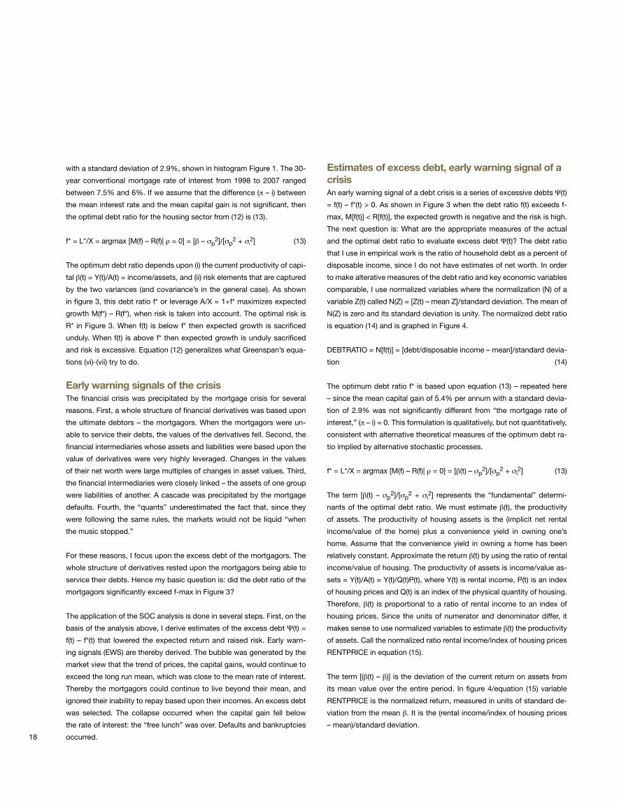
with a standard deviation of 2.9%, shown in histogram Figure 1. The 30-

year conventional mortgage rate of interest from 1998 to 2007 ranged

between 7.5% and 6%. If we assume that the difference (π – i) between

the mean interest rate and the mean capital gain is not significant, then

the optimal debt ratio for the housing sector from (12) is (13).

f* = L*/X = argmax [M(f) – R(f)| ρ = 0] = [β – σp2]/[σp

2 + σi2] (13)

The optimum debt ratio depends upon (i) the current productivity of capi-

tal β(t) = Y(t)/A(t) = income/assets, and (ii) risk elements that are captured

by the two variances (and covariance’s in the general case). As shown

in figure 3, this debt ratio f* or leverage A/X = 1+f* maximizes expected

growth M(f*) – R(f*), when risk is taken into account. The optimal risk is

R* in Figure 3. When f(t) is below f* then expected growth is sacrificed

unduly. When f(t) is above f* then expected growth is unduly sacrificed

and risk is excessive. Equation (12) generalizes what Greenspan’s equa-

tions (vi)-(vii) try to do.

Early warning signals of the crisisThe financial crisis was precipitated by the mortgage crisis for several

reasons. First, a whole structure of financial derivatives was based upon

the ultimate debtors – the mortgagors. When the mortgagors were un-

able to service their debts, the values of the derivatives fell. Second, the

financial intermediaries whose assets and liabilities were based upon the

value of derivatives were very highly leveraged. Changes in the values

of their net worth were large multiples of changes in asset values. Third,

the financial intermediaries were closely linked – the assets of one group

were liabilities of another. A cascade was precipitated by the mortgage

defaults. Fourth, the “quants” underestimated the fact that, since they

were following the same rules, the markets would not be liquid “when

the music stopped.”

For these reasons, I focus upon the excess debt of the mortgagors. The

whole structure of derivatives rested upon the mortgagors being able to

service their debts. Hence my basic question is: did the debt ratio of the

mortgagors significantly exceed f-max in Figure 3?

The application of the SOC analysis is done in several steps. First, on the

basis of the analysis above, I derive estimates of the excess debt Ψ(t) =

f(t) – f*(t) that lowered the expected return and raised risk. Early warn-

ing signals (EWS) are thereby derived. The bubble was generated by the

market view that the trend of prices, the capital gains, would continue to

exceed the long run mean, which was close to the mean rate of interest.

Thereby the mortgagors could continue to live beyond their mean, and

ignored their inability to repay based upon their incomes. An excess debt

was selected. The collapse occurred when the capital gain fell below

the rate of interest: the “free lunch” was over. Defaults and bankruptcies

occurred.

Estimates of excess debt, early warning signal of a crisisAn early warning signal of a debt crisis is a series of excessive debts Ψ(t)

= f(t) – f*(t) > 0. As shown in Figure 3 when the debt ratio f(t) exceeds f-

max, M[f(t)] < R[f(t)], the expected growth is negative and the risk is high.

The next question is: What are the appropriate measures of the actual

and the optimal debt ratio to evaluate excess debt Ψ(t)? The debt ratio

that I use in empirical work is the ratio of household debt as a percent of

disposable income, since I do not have estimates of net worth. In order

to make alterative measures of the debt ratio and key economic variables

comparable, I use normalized variables where the normalization (N) of a

variable Z(t) called N(Z) = [Z(t) – mean Z]/standard deviation. The mean of

N(Z) is zero and its standard deviation is unity. The normalized debt ratio

is equation (14) and is graphed in Figure 4.

DEBTRATIO = N[f(t)] = [debt/disposable income – mean]/standard devia-

tion (14)

The optimum debt ratio f* is based upon equation (13) – repeated here

– since the mean capital gain of 5.4% per annum with a standard devia-

tion of 2.9% was not significantly different from “the mortgage rate of

interest,” (π – i) = 0. This formulation is qualitatively, but not quantitatively,

consistent with alternative theoretical measures of the optimum debt ra-

tio implied by alternative stochastic processes.

f* = L*/X = argmax [M(f) – R(f)| ρ = 0] = [β(t) – σp2]/[σp

2 + σi2] (13)

The term [β(t) – σp2]/[σp

2 + σi2] represents the “fundamental” determi-

nants of the optimal debt ratio. We must estimate β(t), the productivity

of assets. The productivity of housing assets is the (implicit net rental

income/value of the home) plus a convenience yield in owning one’s

home. Assume that the convenience yield in owning a home has been

relatively constant. Approximate the return β(t) by using the ratio of rental

income/value of housing. The productivity of assets is income/value as-

sets = Y(t)/A(t) = Y(t)/Q(t)P(t), where Y(t) is rental income, P(t) is an index

of housing prices and Q(t) is an index of the physical quantity of housing.

Therefore, β(t) is proportional to a ratio of rental income to an index of

housing prices. Since the units of numerator and denominator differ, it

makes sense to use normalized variables to estimate β(t) the productivity

of assets. Call the normalized ratio rental income/index of housing prices

RENTPRICE in equation (15).

The term [(β(t) – β)] is the deviation of the current return on assets from

its mean value over the entire period. In figure 4/equation (15) variable

RENTPRICE is the normalized return, measured in units of standard de-

viation from the mean β. It is the (rental income/index of housing prices

– mean)/standard deviation.

19

N(f*(t)) = [[(β(t) – β]/σ(β) = RENTPRICE (15)

Variable N(f*(t)) in equation (15) corresponds to the optimal debt ratio in

equation (13). Both the actual (DEBTRATIO) and optimal (RENTRPRICE

are graphed in normalized form in Figure 4.

The next question is how to estimate the excess debt Ψ(t). I estimate

excess debt Ψ(t) = (f(t) – f*(t)) by using the difference between two normal-

ized variables N(f(t)) – N(f*(t)), equation (16). This difference is measured

in standard deviations.

Excess debt ~ N[f(t)] – N[f*(t)] = DEBTRATIO - RENTRATIO (16)

Excess debt Ψ(t) corresponds to: (i) the difference [f (t) – f*(t)] on the

horizontal axis in Figure 3, measured in standard deviations, and (ii) the

difference between the two curves DEBTRATIO and RENTPRICE in Fig-

ure 4. The probability of a decline in net worth Pr(dlnX(t) < 0) in (17) is

positively related to Ψ(t) the excess debt for the following reason. As

the excess debt rises, the expected growth declines because risk R(f)

increases relative to M(f) mean in Figure 3.

Pr(d ln X(t) < 0) = H(Ψ(t)), H’ > 0 (17)

Assume that over the entire period 1980 – 2007 the debt ratio was not

excessive. During the period 2000 – 2004, the high capital gains and

low interest rates induced rises in housing prices relative to disposable

income and led to rises in the debt service ratio. By 2005 – 06 the ratio of

housing price/disposable income (PRICEINC in Figure 2) was about three

standard deviations above the long-term mean. This drastic rise alarmed

several economists such as Shiller (2007) who believed that the hous-

ing market was drastically overvalued. As indicated in above, Greenspan

was not unduly concerned with this phenomenon.

The advantages of using excess debt Ψ(t) in Figure 4 as an early warning

signal compared to just the ratio of housing price/disposable income are

that Ψ(t) focuses upon the fundamental determinants of the optimal debt

ratio as well as upon the actual ratio. The probability of declines in net

worth, the inability of the mortgagors to service their debts, and the finan-

cial collapse and a crisis due to leverage are directly related to the excess

debt. In the most general way, Figure 4 should be viewed as follows.

When the DEBTRATIO is above (below) its mean, the RENTPRICE should

be above (below) its mean. When the debt ratio rose significantly above

its mean, were the “fundamentals” measured by RENTPRICE above its

mean? The optimal debt ratio RENTPRICE declined below the mean from

1996 and by 2007 it was 1.5 standard deviations below the mean. The

actual debt ratio DEBTRATIO grew steadily above the mean from 1998

and by 2007 was 2 standard deviations above the mean. Thus the excess

debt grew to 3 standard deviations above the mean from 1998 to 2007.

This is a clear measure of an excess debt and a bubble. The actual debt

was induced by capital gains in excess of the interest rate. The debt

could only be serviced from capital gains. This situation is unsustainable.

When the capital gains fell below the interest rate, the debts could not

be serviced from income. A crisis was inevitable. Thus the excess debt in

Figure 4 was an early warning signal of a crisis.

ConclusionAlan Greenspan’s paper presented his retrospective view of the crisis.

Two main themes emerge. First, the housing price bubble, its subse-

quent collapse and the financial crisis were not predicted either by the

market, the Fed, the IMF or the regulators in the years leading to the

current crisis. Second, the Fed, IMF, Treasury and the “quants”/market

lacked the appropriate tools of analysis to answer the following ques-

tions: what is an optimal leverage or capital requirement that balances

the expected growth against risk? What are theoretically founded early

warning signals of a crisis? What lessons should be learned?

The Fed apparently lacked adequate tools which might have indicat-

ed that asset values were vastly out of line with fundamentals. They

were not searching for such tools because they did not believe that

they could or should look for misaligned asset values or excess debt,

despite warnings from Shiller and some people in the financial indus-

try. They were blindsided by the Jackson Hole Consensus which gave

them great comfort in adopting a hands off position. So it was not just

a lack of appropriate tools which undid the Fed; it was a complete lack

of appreciation of what its role should be to head off an economic catas-

trophe. There are two separate but related questions: are identification

and containment of a financial bubble legitimate activities of the Fed,

and if they are, what are the best tools to carry out this analysis? As the


-2

-1

0

1

2

3

80 82 84 86 88 90 92 94 96 98 00 02 04 06

RENTPRICE

DEBTRATIO

Figure 4Early warning signals: Excess debt Ψ(t) = N[f(t)] – N[f*(t)].

N[f(t)] = DEBTRATIO = (household debt as percent of disposable income – mean)/standard

deviation. N[f*(t)] = RENTPRICE = (rental income/housing price index – mean)/standard

deviation.

Source: FRED

20

Fed answered “no” to the first question, it saw no need to address the

second question.

The Jackson Hole Consensus explains to a considerable extent the Fed’s

behavior. Greenspan has great knowledge of financial markets and did

have some qualms about the housing boom. I think that his behavior

can be explained rationally. First, he understands that the function of

financial markets is to channel saving into investment in the optimal

way to promote growth. Second, like most of the economics profession,

he accepted the generality of the First Theorem of Welfare Economics.

This theorem [Koopmans and Bausch (1959)] states that a competitive

equilibrium is a Pareto optimum. A competitive equilibrium is a vector of

prices, where (i) supply equals demand, (ii) consumers optimize demand

and their supply of labor services, given their preferences and (iii) produc-

ers optimize by maximizing their profits, given the technology. A Pareto

optimum is a vector of choices such that (iii) supply equals demand and

(iv) it is not possible to select vectors which would make some people

better off without making others worse off. The implication is that “market

regulation” is superior to regulation by bureaucrats and politicians. Do

not try to second guess the markets.

The belief in the generality of the First Theorem of Welfare provided a ba-

sis for Greenspan’s position. The theorem does not hold in financial mar-

ket because the assumption of atomistic agents operating in perfectly

competitive markets with full information and stable preferences is wildly

unrealistic. The clearly imperfect markets operating with agents acting

without full information concerning the values of the complex derivatives,

in fact almost complete ignorance, implies the conclusion that the situa-

tion before the crash cannot be considered to be a Pareto optimum.

When the crash occurred, Greenspan (2008) wrote, “Those of us who

have looked to the self-interest of lending institutions to protect stock-

holders’ equity, myself included, are in a state of disbelief.” To his great

credit, in his retrospective Greenspan qualified his trust in financial mar-

kets to optimally allocate resources by advocating minimum capital re-

quirements or maximum leverage. His object was to have a minimum

capital requirement to yield a rate of return on equity sufficient to provide

the financial sector with resources to promote growth. The proposals for

reform and the regulators ignore this and just focus upon some arbitrary

risk measures.

Greenspan’s formulation is a step in the right direction, however, there

are several limitations to his formulation. There is no explicit trade off be-

tween growth and risk. Risk is not explicit in his formulation. His required

minimum return on equity is arbitrary and lacks theoretical foundations.

His formulation says nothing about the effects upon risk and growth of

leverage or capital requirements that deviate from the value from his de-

rived estimate.

The stochastic optimal control analysis attempts to rectify these diffi-

culties. I drive an optimal debt ratio or leverage or capital requirement

that optimally balances expected growth against risk, in an environment

where the capital gain and interest rate are stochastic. The stochastic

optimal control analysis developed here derives a time varying optimal

debt ratio. The crucial variable is the excess debt, the difference between

the actual and optimal debt ratio. (1) The optimum debt ratio or leverage

maximizes the expected growth of net worth. (2) As the excess debt ratio

rises, the expected growth of net worth declines and the risk rises. (3) The

probability of a crisis is positively related to the excess debt, measured

in standard deviations. When the leverage exceeds a specified value,

the expected growth of net worth is negative and the risk is high. (5) The

derived early warning signal, the excess debt ratio, would have clearly

predicted the crisis, as shown in Figure 4.

Peter Clark (2009) wrote: “no measure of underlying or fundamental value

will provide consistently accurate predictions of emerging bubbles, but

the prior question is whether it is useful to even contemplate the exer-

cise of assessing market values. In light of the huge costs of the hous-

ing and credit bubble, the answer must be in the affirmative.” Fed Vice

Chairman Kohn indicated that the Fed’s thinking may have changed. He

wrote (2009, quoted by Clark): “As researchers, we need to be honest

about our very limited ability to assess the ‘fundamental value’ of an as-

set or to predict its price. But the housing and credit bubbles have had

a substantial cost. Research on asset prices … should help to identify

risks and inform decisions about the costs and benefits from a possible

regulatory or monetary policy decision attempting to deal with a potential

asset price bubble.”

21

References• Bernanke, B., 2005, Testimony to Congress Joint Economic Committee, October

• Borrio, C., and P. Lowe, 2002, “Asset prices, financial and monetary stability,” BIS Working

paper #114

• Burry, M. J., 2010, “I saw the crisis coming. Why didn’t the Fed?”, New York Times, April 4,

2010, Op/Ed page

• Clark, P., 2009, “Comment on tale of two debt crises”, Economics, The Open-Assessment

E-Journal, http://www.economics-ejournal.org/economics/discussionpapers/2009-44.

• Congressional Oversight Panel, 2009, “Special report on regulatory reform,” Washington D.C.,

January

• Demyanyk, Y., and O. Van Hemert, 2007, “Understanding the subprime mortgage crisis,”

SSRN: <http://ssrn.com/abstract=1020396>

• FRED, Federal Reserve Bank St. Louis, Economic data set

• Fleming, W. H. and J. L. Stein, 2004, “Stochastic optimal control, international finance and

debt,” Journal of Banking and Finance, 28 , 979-996

• Gerardi, K., A. Lehnert, S. Sheelund and P. Willen, 2008, “Making sense of the subprime crisis,”

Brookings Papers, Fall

• Greenspan, A., 2004a, Understanding household debt obligations, Remarks at Credit Union

National Association, Washington, D.C., February 23

• Greenspan, A., 2004b, The mortgage market and consumer debt, Remarks at America’s

Community Bankers Annual Convention, Washington DC, October 19

• Greenspan, A., 2008, Testimony on sources of financial crisis, House Committee on

Government Oversight and Reform

• Greenspan, A., 2010, “The crisis,” Brookings Papers, second draft

• International Monetary Fund, 2007, “World economic and financial survey,” Global financial

stability report

• Issing, O., 2010, “Some lessons from the financial crisis,” International Finance, 12:3, 431-44

• Koopmans, T., and A. Bausch, 1959, Selected topics in economics involving mathematical

reasoning, SIAM Review, 1:2, 79-148

• Lowenstein, R., 2010, The end of Wall Street, Penguin Press, New York

• OFHEO, 2010, House price indexes, Washington, D.C.

• Shiller, R., 2007, “Understanding recent trends in house prices and home ownership,” Cowles

Foundation Discussion Paper #1630

• Shojai, S., and G. Feiger, 2010, “Economists’ hubris – the case of risk management,” Journal

Financial Transformation, 28, 25-35

• Stein, J. L., 2005, “Optimal debt and endogenous growth in models of international finance,”

Australian Economic Papers, Special Issue on Stochastic Models, 44, 389-413

• Stein, J. L., 2006, Stochastic optimal control, international finance and debt crises, Oxford

University Press

• Stein, J. L., 2010, “A tale of two debt crises: a stochastic optimal control analysis,” Economics/

The Open-Access, Open-Assessment E- journal, vol. 4 – 2010-3 <http://www.economics-

ejournal.org/economics>


22

23

PART 1

Share Price Disparity in Chinese Stock Markets1

AbstractThe presence of price disparity between A- and H-shares

suggests that the two markets are segmented and thus al-

location of capital is inefficient. In this paper, we attempt to

identify the factors contributing to the price disparity, with a

view to helping policymakers find solutions to the problem.

Our results suggest that the disparity is caused by a com-

bination of micro and macro factors. Some of these factors

are found to have played a crucial role in determining the

disparity, implying that removing or reducing the segmenta-

tion can potentially bring considerable benefits by improving

price discovery and market efficiency.

Tom Fong — Manager, Research Department, Hong Kong Monetary Authority

Alfred Wong — Senior Manager, Research Department, Hong Kong Monetary Authority

Ivy Yong — Senior Manager, Research Department, Hong Kong Monetary Authority

1 This article is also published as Chapter 10 of Genberg, H. and D. He (eds.)

2008, Macroeconomic linkages between Hong Kong and Mainland China,

City University of Hong Kong Press.

24

The presence of persistent price disparity between A- and H- shares

suggests that the two markets are segmented and thus allocation of

capital is inefficient. In this paper, we attempt to answer probably the

most fundamental question on the phenomenon, identifying the factors

contributing to the price disparity, with a view to helping policymakers

find solutions to the problem. This paper complements the analysis of

the changes in the price disparity by Peng et al. (2007).2

Internationally, when price disparity exists between two shares of the

same stock, the one accessible by foreign investors usually commands

a premium over the one restricted only to domestic ownership. However,

almost all H- shares, which are accessible by foreign investors, are trad-

ed at a discount to their counterparts in the A-share market on the Main-

land. Nonetheless, this should not be seen as an inconsistency because

in most other emerging markets shares accessible by foreign investors

are also open to domestic investors – which leaves no opportunity for

any discount to exist – while in the Chinese case foreign and domestic

investors do not have access to each other’s markets.3

Whether one tries to explain a premium (in the case of other emerging

markets) or a discount (in the case of the Chinese markets) should not

have any implications for the approaches adopted in empirical studies.

Previous studies on price disparity in segmented stock markets are fairly

diverse in terms of model specification, due to different hypotheses or

explanations. However, despite the diversity, the hypotheses or explana-

tions focus mainly on five factors, namely, market liquidity, shares supply,

market risk, information asymmetry, and general market conditions – in

particular in those studies of the Chinese markets (Table 1). All of these

are plausible factors contributing to the stock price disparity from a micro

perspective. No empirical work has, according to our knowledge, con-

sidered the channels through which recent macroeconomic imbalance of

China’s economy has played an increasingly important role.

The macroeconomic imbalance has arguably impacted the prices of the

A- and H-share markets, and hence their disparity, in at least three ways.

First, an undervalued currency and thus expectations of future revalua-

tion or appreciation have provided strong motivation for foreign investors

to acquire H-shares as a proxy for “renminbi” assets, though H-shares,

which are denominated in Hong Kong dollars, are not renminbi assets

per se. Second, the external imbalance resulting from an undervalued

renminbi has been manifested into rising internal imbalance as evidenced

by rapidly growing bank deposits. With limited choice of financial prod-

ucts available domestically, stock investments, in addition to real estate

investments, have offered a convenient and feasible alternative to bank

deposits for the majority of mainland investors. Finally, as China’s trade

surplus continues to rise, the opportunities for mainlanders to retain their

foreign currency proceeds outside the mainland to avoid capital controls

have increased. This in turn reflects increased ability of mainlanders to

arbitrage by purchasing the H-share of the same stock whenever they

find the discount offered by the H-share attractive enough.

Preliminary analysisBoth the price and quantity data of A- and H-shares are monthly aver-

ages of daily data extracted from Bloomberg, covering the period from

April 2000 to February 2007.4 It is useful to note that this period saw

significant growth in the market, with the number of dual-listed stocks

more than doubling from 17 to 36 (Table 2) and, even after controlling for

price increases, the size of the market capitalization had expanded 16

times.5 In Figure 1, we plot the indices of the market capitalization of the

dual-listed A- and H-shares over time, with all stock prices held constant

at their February 2007 levels. As can be seen, in April 2000 the A- and

H-share markets – controlled for price changes – were only about 6% of

the market size reached in February 2007. This is particularly important

when comparing results with previous studies, because the A-H market

today is quite different from what it used to be in the 1990s (covered by

most other studies).

Next, we compute the Divisia (1925) indices, correlations, and variances

of the A- and H-shares to provide a simple view of the relationship be-

tween their respective returns over time.6 When applied in the current

context, the Divisia price index is a market-capitalization-weighted av-

erage of logarithmic price changes (returns). In the computation, share

prices are adjusted for changes in the exchange rate. Figure 2 presents

the scatter plot of the Divisia A- and H-share price indices where each

point corresponds to a specific month. The dispersion of the Divisia A-

relative to H-share price index and their deviations from the 45-degree

line reflect the degree of segmentation between the two markets. There

appears to be only a mild positive relationship between the returns of

A- and H-shares. This is consistent with Figure 3 which shows that the

two indices exhibit a slight tendency to move in tandem, especially from

around 2003 Q3.

2 While identifying the factors affecting the price disparity can also shed light on the changes

in the price disparity, the latter paper differs in that it studies the changes or dynamics by

examining the statistical properties of the disparity itself.

3 Foreign investors have in recent years been able to access the A-share market via the

qualified foreign institutional investors scheme but the access has remained very limited.

During the period under study, the qualified domestic institutional investors scheme was

limited to fixed income products and there was no formal channel for mainland investors

to access the H-share market. However, it was recently announced that this rule will be

relaxed, allowing mainland investors to invest in overseas equities.

4 The earliest available record for all 17 stocks on Bloomberg is April 2000, although the his-

tory of dual-listed A- and H-shares dates as far back as 1993. There are two reasons for

not covering the whole dual-listing history in this study. First, we want to maintain a higher

degree of data consistency by using one data source. Second, and more importantly, the

market in the 1990s was too small (compared to the market today) to have any useful

policy relevance.

5 Since February 2007, the number of dual-listed stocks has increased to 39.

6 We employ the Divisia index instead of other more commonly used indices such as the

Paasche, Laspeyre and Fisher indices, because its higher-order moments can capture the

relationship among individual stock price changes while others cannot.

25

The Divisia A-H share correlation shows the co-movement between A-

and H-shares. As can be seen in Figure 4, their relationship is found to

be positively correlated in most of the period. It is also noted that the

Divisia correlation averaged about 0.2 initially and then trended higher

from around the beginning of 2003, reaching about 0.6 by the end of the

period. Hence, gradual integration between the two markets seems to

have taken place over the past four years. This result is consistent with

the finding of Peng et al. (2007) that there was relative price convergence

between the A- and H-shares of the dual-listed stocks.

The Divisia variance is the second-order moment of individual stock pric-

es, which measures the extent to which the prices of individual stocks

change disproportionately. In other words, it is a measure of relative price

changes, not absolute price changes. When all prices change by the

same proportion, it vanishes. Scatter plots of the monthly Divisia A- and

H-share price variances for the past seven years are presented in Fig-

ure 5, with the top panel including all observations and the bottom panel

excluding the outliers defined as larger than 0.01. In both cases, there are

about two-thirds or 66% of observations lying above the 45-degree line.

In other words, for the dual-listed stocks, A-shares tend to have a smaller

Divisia variance than do H-shares, indicating that the prices of A-shares

tend to move more in tandem, when compared with those of H-shares.

There must exist some common forces that drive stock prices in the A-

share market to go in one direction or the other, resulting in a smaller

dispersion of price movements. What could these common forces be?

The rest of the paper will shed some light on this question.

Model specificationTo examine the relevance of the various possible factors leading to the

price disparity, we employ a fixed effect panel data model in our estima-

tion. A panel data model allows us to analyze the disparity for a large

number of firms simultaneously using time series data, while a fixed ef-

fect structure can help control for unobservable firm-specific effects, so

that differences across companies can be captured.7 Specifically, the re-

gression model is as follows:

PREMit = α0 + α1LQit + α2SPit + α3RKit + α4INFit + α5MCit + α6CURit +

α7M2it + α8TRit + α9PREMit-1 + ηi + εit (1)

where subscripts i and t denote stock i and time t respectively. The

Author(s) Markets No. of Firms Period Factors

Ng and Wu (2007) A-shares 32% of total market turnover trade on SH 2001-2002 Risk, market conditions

Guo and Tang (2006) A- versus H-shares 29 A/H shares 1993-2003 Cost of capital, liquidity

Chan and Kwok (2005) A- versus H-shares and

A- versus B-shares

13 A/H shares

41 A/B shares

1991-2000 Liquidity, supply, risk, information asymmetry

Wang and Li (2003) A- versus H-shares 16 A/H shares 1995-2001 Liquidity, risk, market conditions, exchange rate

Fung et al. (2000) A- versus B-shares 20 A/B shares 1993-1997 Dividend yield, exchange rates, bond yield

Sun and Tong (2000) A- versus B-shares

A- versus H-shares

45 A/B shares

10 A/H shares

1994-1998 Risk, bond issued, number of listed firms, information asymmetry,

foreign reserves, inflation, liquidity

Su and Fleisher (1999) A- versus B-shares 24 A/B shares 1993-1997 Risk, number of investors, information asymmetry

Chakravarty et al. (1998) A- versus B-shares 39 A/B shares 1994-1996 Risk, information asymmetry, supply

Ma (1996) A- versus B-shares 38 A/B shares 1992-1994 Market conditions, Chinese deposit rates, CPIs of China and U.S.

Chen et al. (2001) A- versus B-shares 36 (SHSE) and 32 (SZSE) A/B shares 1992-1997 Risk, information asymmetry, liquidity

Bailey (1994) A- versus B-shares 14 A/B shares 1992-1993 Market conditions

The above summary focuses on the modeling of the cross-sectional data in panel data analysis. In the literature, the liquidity factor is represented by the trading volume (or the ratio to market

capitalization or the ratio to total trading volume) and bid-ask spread. The risk factor is represented by the volatility of prices and variance-covariance ratios. The supply factor is represented by the

total outstanding shares and tradable market shares. The information asymmetry factor is reflected by total market capitalization. The factor of market conditions is proxied by the market returns.

Table 1 – Literature review on Chinese stock markets

7 See Domowitz (1997) and Hsiao (1986) for details.

The Capco Institute Journal of Financial TransformationShare Price Disparity in Chinese Stock Markets

0%

20%

40%

60%

80%

100%

Ap

r-00

Jul-

00

Oct

-00

Jan-

01

Ap

r-01

Jul-

01

Oct

-01

Jan-

02

Ap

r-02

Jul-

02

Oct

-02

Jan-

03

Ap

r-03

Jul-

03

Oct

-03

Jan-

04

Ap

r-04

Jul-

04

Oct

-04

Jan-

05

Ap

r-05

Jul-

05

Oct

-05

Jan-

06

Ap

r-06

Jul-

06

Oct

-06

Jan-

07

% (A-shares)

% (H-shares)

Figure 1 – The market capitalization (Feb 2007 = 100%)

26

No Company H-shares ticker A-shares ticker

1 Luoyang Glass 1108 600876

2 Nanjing Panda 553 600775

3 Northeast Electric 42 000585

4 Shandong Xinhua Pharmaceutical 719 000756

5 Sinopec Yizheng Chemical Fibre 1033 600871

6 Beijing North Star 588 601588

7 Beiren Printing Machinery 187 600860

8 Jingwei Textile Machinery 350 000666

9 China Eastern Airlines Corp 670 600115

10 Tianjin Capital Environmental

Protection

1065 600874

11 Guangzhou Pharmaceutical 874 600332

12 Sinopec Shanghai Petrochemical 338 600688

13 Jiangxi Copper 358 600362

14 China Southern Airlines 1055 600029

15 Guangzhou Shipyard International 317 600685

16 China Petroleum & Chemical Corp 386 600028

17 Guangshen Railway 525 601333

18 Jiaoda Kunji High-Tech 300 600806

19 Dongfang Electrical Machinery 1072 600875

20 Air China 753 601111

21 Bank of China 3988 601988

22 Datang International Power Generation 991 601991

23 ZTE Corp 763 000063

24 Jiangsu Expressway 177 600377

25 Maanshan Iron & Steel 323 600808

26 Yanzhou Coal Mining 1171 600188

27 Industrial and Commercial Bank of

China

1398 601398

28 Tsingtao Brewery 168 600600

29 Shenzhen Expressway 548 600548

30 Anhui Conch Cement 914 600585

31 Huadian Power International Corp 1071 600027

32 China Shipping Development 1138 600026

33 Anhui Expressway 995 600012

34 Angang Steel 347 000898

35 Huaneng Power International 902 600011

36 China Merchants Bank Co. Ltd. 3968 600036

Table 2 – The 36 selected companies commonly listed in both markets

dependent variable PREM represents the price disparity of stock i, de-

fined as the price premium of stock i in the market of A-shares over the

same stock in the market of H-shares at time t. LQ, SP, RK, INF, and MC

denote respectively the five popular factors identified in previous studies,

namely, liquidity, supply, risk, information asymmetry, and market condi-

tions of the two markets (all in relative terms). To take into account the

indirect impact of the macroeconomic imbalance, we introduce into the

model three other variables CUR, M2, and TR, which denote the 3-month

-25%

-20%

-15%

-10%

-5%

0%

5%

10%

15%

20%

25%

-25% -20% -15% -10% -5% 0% 5% 10% 15% 20% 25%

DIV A

DIV H

Figure 2 – Scatter plot of Divisia indices (monthly)

-20%

-15%

-10%

-5%

0%

5%

10%

15%

20%

25%

Jan-

00

Jul-

00

Jan-

01

Jul-

01

Jan-

02

Jul-

02

Jan-

03

Jul-

03

Jan-

04

Jul-

04

Jan-

05

Jul-

05

Jan-

06

Jul-

06

Jan-

07

Div A Div H

Figure 3 – Divisia indices (monthly)

-0,40

-0,20

0,00

0,20

0,40

0,60

0,80

1,00

Jan-

00

May

-00

Sep

-00

Jan-

01

May

-01

Sep

-01

Jan-

02

May

-02

Sep

-02

Jan-

03

May

-03

Sep

-03

Jan-

04

May

-04

Sep

-04

Jan-

05

May

-05

Sep

-05

Jan-

06

May

-06

Sep

-06

Jan-

07

May

-07

Divisia Corr Trend

Figure 4 – Divisia correlations (monthly)

27


renminbi non-deliverable forward (NDF) rate, money supply M2 of the

mainland, and the trade balance of the mainland respectively.8

The lagged price premium is included to reflect the trend of the price

premium and filter out the autocorrelation [Domowitz et al. (1997)].9 The

coefficient vector α = (α0, α1, …, α9)’ is fixed over time and across stocks

by assumption.10 The variables ηi are the individual effects capturing the

unobserved idiosyncratic features of stock i and the variables εit are the

disturbances.

Table 3 provides the data details of each explanatory variable used in

the estimation. For each stock, the price premium PREM is measured by

the logarithmic value of the average monthly A-share price PA minus that

of the average monthly H-share price, i.e., PREM = log(PA) – log (PH).11

The liquidity factor LQ is proxied by the relative turnover rates of the two

8 To avoid the problem of collinearity between levels of money supply of China and ren-

minbi’s NDF rate, which are shown to be monotonic increasing, the ratios of the current

value over its lag Xt/Xt-1 (i.e., with the variables in change form instead of level when taking

logarithm) are considered in the estimation.

9 The correlation between the lagged dependent variable and the disturbance gives rise to

the biased estimation of coefficients under ordinary least squares estimation. We employ

a generalized method of moment (GMM) estimator to correct the standard errors for

heteroskedastickity of unknown form in the time-varying error components and to permit

efficient estimation.

10 A random effect model, which allows the individual specific effect to change over time,

may provide a better explanatory power for the price premium over the fixed effect model.

However, the Hausman test suggests that there is no significant difference between the

two model specifications. Moreover, the number of parameters increases sharply when the

random effect model is considered, which is especially unfavourable for the scarcity of data

on the time dimension. In view of this, the fixed effect model is chosen.

11 All A-share prices originally denominated in renminbi are converted to Hong Kong dollar.

Variable Type of Variable / Factor Description Expected

effect

PREMt Dependent variable Natural logarithm of A-share price minus natural logarithm of H-share price of the same stock

LQ Liquidity Monthly trading volume to the total number of shares outstanding in the A-share market over monthly trading volume to the total

number of shares outstanding in the H-share market (in natural logarithm)

+

SP(1) Supply (1) Natural logarithm of number of free-floating shares in the A-share market over number of free-floating shares in the H-share

market

-

SP(2) Supply (2) Natural logarithm of number of outstanding shares in the A-share market over number of outstanding shares in the H-share

market

-

RK Risk level Natural logarithm of 30-day annualized standard deviation of A-shares over 30-day annualized standard deviation of H-shares +

INF(1) Information asymmetry (1) Natural logarithm of total market capitalization based on all free-floating shares listed in the A-share and H-share markets -

INF(2) Information asymmetry (2) Natural logarithm of total market capitalization based on all outstanding shares listed in the A-share and H-share markets -

MC Market conditions Natural logarithm of Shanghai Stock Index over Hang Seng Index +

CUR Rate of renminbi

appreciation

Natural logarithm of 3-month nondeliverable forward contract of renminbi over its lag -

M2 Growth of China’s money

supply

Natural logarithm of China’s money supply (M2) over its lag +

TR Trade balance Natural logarithm of total export over total import in China -

PREMt-1 Lagged term The price premium in the previous month +

Table 3 – Description of the dependent variable and explanatory variables

0,000

0,005

0,010

0,015

0,020

0,000 0,005 0,010 0,015 0,020

Divisia Variance of H Share

Divisia Variance of A Share

0,000

0,005

0,010

0,000 0,005 0,010

Divisia Variance of H Share

Divisia Variance of A Share

Figure 5 – Scatter plot of Divisia variances

28

markets, where the turnover rate is defined as the monthly trading volume

to the total number of shares outstanding in the markets.12,13 To reflect the

relative supply of the two markets, two proxies, namely, (i) the ratio of the

number of free-floating A-shares to the number of H-shares (denoted by

SP(1)) and (ii) the ratio of the number of outstanding A-shares to the num-

ber of outstanding H-shares (denoted by SP(2)), are considered.14 The ratio

of the variances of returns is used to reflect the relative risk levels RK.15

Information asymmetry is proxied by the relative market capitalization of

free-floating shares (denoted by INF(1)) and that of total outstanding shares

(denoted INF(2)) of the two markets.16 Some descriptive statistics of the

variables are presented in Tables A1 and A2 in the Appendix.

Empirical resultsEquation (1) is estimated by the generalized method of moments (GMM)

so that it can avoid any bias when variables are endogenous.17 Two re-

gression models, models A and B, are estimated. Model A is (1) using

SP(1) and INF(1) as the supply and information asymmetry variables re-

spectively and is estimated for the period from October 2005 to February

2007.18 Model B is the same as model A except that SP(2) and INF(2) are

used as the supply and information asymmetry variables respectively.

Given that more data are available for SP(2) and INF(2), model B is esti-

mated for a longer period from April 2000 to February 2007. Both models

have their advantages because model A contains variables that are argu-

ably more able to capture the effects of supply and information asym-

metry, while model B covers a longer period.

The estimation results are reported in Table 4. The Portmanteau test

statistics show that the residuals of the two models have insignificant

serial correlation, suggesting that both models are adequately fitted.19

The coefficients have same signs in both models, except that information

asymmetry in model B is found to be different from that in model A. Our

key findings for each variable are discussed below.

On the five popular factors identified from the literature■■ The price premium is positively related to the relative liquidity of

A-shares over H-shares (LQ). This finding suggests that a more liquid

A-share (H-share) market tends to increase (reduce) the price pre-

mium and vice versa. This is consistent with the theoretical prediction

– that investors tend to demand a smaller (larger) compensation for

12 Such measures are commonly used in the literature and they are more powerful in explain-

ing price discounts than others in empirical analysis [see Ma (1996), Domowitz et al. (1997),

and Wang and Li (2003)]. The bid-ask spread is also a natural proxy of liquidity [Guo and

Tang (2006)]. However, Amihud and Mendelson (1986) found that asset returns are an

increasing and concave function of the spread. Consequently, some nonlinear properties

should be imposed in the model when the bid-ask spread is used in the estimation.

13 A joint cross-correlation test is considered to examine the lead-lag relationship between

the price premium and the turnover rate (i.e., the proxy of liquidity ratio). The joint cross-

correlation test shows that the price premium leads the turnover rate significantly, while the

turnover rate does not lead the price premium significantly. These results suggest that the

issue of reverse causality (i.e., turnover rate leading price premium) is not significant in the

analysis.

14 The free-floating H-shares is defined as the number of shares that are available to the pub-

lic, while the free floating A-shares is defined as the number of current shares outstanding

that are tradable or listed on the stock exchange.

15 They are the 30-day price volatility which equals the annualized standard deviation of rela-

tive price change of the 30 most recent trading days’ closing price. The volatility is the

standard deviations of day-to-day logarithmic price changes.

16 Since larger firms have more information disclosure, the firm size proxied by the market

value of total outstanding shares may reflect the availability of information. Chan and Kwok

(2005) commented that the market capitalization of total shares outstanding may also be

a good indicator of the availability of information on the firm. However, their estimation

results suggested that the market capitalization of free-floating shares is a better indicator

to reflect such factor.

17 In the estimation, we transform equation (1) into first differences with the “white period

GMM weight,” which provides correct estimates of the coefficient covariances in the pres-

ence of heteroskedasticity of unknown form.

18 Such information is only available since October 2005.

19 All residuals of model A have insignificant correlations at a 0.05 level of significance. In

model B, all but two firms’ residuals have insignificant correlations at an 0.05 level of sig-

nificance. The two firms are found to have significant correlations among residuals because

there were some violent fluctuations during early 2000. As the majority of the firms have

already passed the Portmanteau test and the hypotheses for two firms are just marginally

rejected, no dummy variable is introduced in the model.

Model A Model B

Oct 2005 – Feb 2007 Apr 2000 – Feb 2007

Variable Coefficient Coefficient

LQ 0.0417a 0.0322a

SP(1) -0.0779b

SP(2) -0.2081a

RK 0.0300b 0.0051

INF(1) -0.1227a

INF(2) 0.0728c

MC 0.3300a 0.3478a

CUR -4.8083a -1.8233a

M2 0.7166a 0.5178a

TR -0.0164 -0.0008

PREM(t-1) 0.1911a 0.2931a

Portmanteau

test statistics

Q(6) for all

stocks 2, 3

4.9, 4.5, 5.7, 5.0, 12.0, 1.5, 7.0,

3.8, 10.5, 4.3, 6.2, 7.2, 4.6, 3.9,

4.4, 4.8, (X), 4.0, 1.8, 6.4, 7.1, (X),

2.8, 2.4, 5.7, 5.9, 2.0, 3.2, 2.1,

7.5, 11.8, 7.9, 4.2, 4.5, 6.5, 2.5.

4.6, 5.2, 8.9, 5.1,10.6, 1.2, 4.4,

2.4, 9.3, 9.8, 9.9, 12.2, 1.9, 12.4,

3.3, 10.3, (X), 16.6, 5.9, 2.1, 6.2,

(X), 5.3, 8.7, 4.9, 7.9, 2.0, 2.2, 2.2,

8.2, 7.0, 2.7, 2.5, 18.5, 9.5, 3.7.

No. of stocks 36 36

No. of obs. 482 2039

Notes:

1. a, b, and c denote significance at the 1 percent, 5 percent and 10 percent levels

respectively.

2. The Portmanteau test, Q(K), checks whether residuals of each firm are jointly zero

correlated up to lag K. At 0.05 and 0.01 level of significance, the critical values are 12.6

and 16.8 respectively. Their corresponding stocks (tickers) are: 1108, 553, 42, 719, 1033,

588, 187, 350, 670, 1065, 874, 338, 358, 1055, 317, 386, 525, 300, 1072, 753, 3988, 991,

763, 177, 323, 1171, 1398, 168, 548, 914, 1071, 1138, 995, 347, 902, 3968.

3. (X) denotes that the corresponding stocks are deleted due to missing information in the

final estimation.

Table 4 – Determinants of price premium: GMM estimates

29

lower (higher) trading cost associated with a more (less) liquid market

– as well as the findings in other empirical studies.20

■■ The price premium is found to be negatively associated with the

relative supply of A-shares over H-shares (SP) in model A. This result

highlights the relative scarcity of A- over H-shares as an important

factor in explaining the price premium, reflecting the lack of substi-

tutes for stock investment on the mainland.

■■ The price premium is positively related to the relative risk ratio (RK)

in both models. This result supports the differential risk hypothesis,

which postulates that the price premium can be explained by the

relative riskiness of the assets because the A- and H-share investors

have different risk profiles. Market commentaries often suggest that

mainland investors are more speculative (having a higher risk appetite

or being less risk averse) and hence may be more willing to pay a

higher price for an asset with the same level of risk. On the other hand,

Hong Kong and international investors tend to be relatively more risk-

averse. Our estimation finds the price premium to be larger for stocks

with higher price volatilities in their A-shares than in their H-shares.

■■ Our results provide some but limited support for the information

asymmetry (INF) hypothesis. This hypothesis states that price dispar-

ity can be explained by information asymmetry, which can be caused

by factors such as availability of reliable information, speed of infor-

mation flows, language barriers, and different accounting standards.

Information asymmetry may result in certain group of investors being

disadvantaged and thus less willing to pay. Many studies in the litera-

ture employ firm size as a proxy for asymmetric information because

larger firms tend to have better information disclosure and attract

more analysts to study their stocks. In model A, the results for the

more recent period show that larger firms tend to have lower price

disparities. However, model B yields an opposite outcome. This may

suggest that information asymmetry has become a relevant factor

only recently, possibly attributable to the listing of some very large

firms during 2006.

■■ Market conditions (MC) is found to be positively significant in both

models. The stock market indices of the mainland and Hong Kong are

used as proxies for market conditions, to capture the effects of both

market sentiment and general economic conditions, which in turn can

have an impact on corporate performance.21

On the effects of the macroeconomic imbalance■■ Renminbi revaluation or appreciation (CUR) has a negative relation-

ship with the price premium. Appreciation or expected appreciation

of the renminbi increases the value of renminbi-denominated assets

in U.S. dollars. Given current capital controls of the mainland,

H-shares remain the most direct and convenient way for foreign

investors to acquire mainland or renminbi-income-generated assets.

Consequently, H-share prices should reflect the effect of renminbi

appreciation on the firm’s future earnings. The results suggest that

an appreciation or expected appreciation of the currency induces

H-share purchases, thus squeezing the price premium.22

■■ Money supply (M2) is found to be positively related to the price premi-

um.23 As the macroeconomic imbalance grows, money supply grows.

The range of financial products available for investment or savings is,

however, very limited on the mainland. With deposit rates kept very

low for a long time, stocks have become an increasingly attractive

investment option. The macroeconomic imbalance has thus indirectly

contributed to the demand for local stocks, which have translated into

higher A-share prices and large premiums over H-shares. Our results

here simply confirm a widely-observed phenomenon.

■■ The trade balance (TR) is estimated to be negative, though the coef-

ficients are insignificant. It is common knowledge that trade flows are

often used to camouflage capital flows in the presence of capital con-

trols. The trade surplus, which can capture the opportunities of main-

landers to keep their foreign exchange earnings outside the country,

is used here to proxy the ability of mainland investors to arbitrage the

price differentials of dual-listed A-H stocks in the H-share market.

As a result, a rising trade surplus has the effect of lifting the price of

H-shares, thus reducing the A-share price premium. The insignificant

coefficient may, however, suggest that despite the large trade surplus

the impact of mainland investors on H-share prices remains limited.

■■ The coefficient of lagged price premium is estimated to be less than

unity, indicating that share price differentials were partially adjusted

over the period when other variables are kept constant.

Final remarksDual-listed A- and H-shares came into being as soon as the mainland

authorities allowed mainland companies to be listed in the Hong Kong

stock market in the early 1990s. For more than a decade there has ex-

isted a persistent premium of the A-share over the H-share for the same

stock. Initially, dual-listed A- and H- shares were mostly small mainland

companies, but the last two years saw phenomenal growth of this mar-

ket segment following the listing of some very large companies. As a

result, the A-H share price disparity has attracted increasing attention


20 Chen et al. (2001), Wang and Li (2003), and Chan and Kwok (2005) find positive relation-

ships between A-share price premium and relative trading volume/turnover rates of A- over

H-shares. The results of Guo and Tang (2006) show a negative relationship between

A-share price premium and the relative bid-ask spread of A-H shares – more liquid markets

tend to have narrower spreads.

21 Based on historical data, the pairwise correlation between the changes in the H-share

prices and the changes in the Hang Sang Index is 0.15, while that between the changes in

the H-share prices and the changes in the Shanghai Stock Index is 0.21. These figures sug-

gest that both markets’ investment environment may somewhat affect the H-share prices.

Better Hong Kong stock market conditions may stimulate market sentiment and provide

more incentives for investors to buy discounted H-share stocks so that the price premium

will narrow.

22 Note that the A-shares can only be traded by mainland investors.

23 Bank deposits, including demand deposits, time deposits, and saving deposits, were also

considered in the initial estimations. All results were of similar flavor.

30

References• Amihud, Y. and H. Mendelson, 1986, “Asset pricing and the bid-ask spread,” Journal of

Financial Economics 17:2, 223-249

• Bailey, W., 1994, “Risk and return on China’s new stock markets: some preliminary evidence,”

Pacific-Basin Finance Journal, 2, 243-260

• Chakravarty, S., A. Sarkar, and L. Wu, 1998, “Information asymmetry, market segmentation and

the pricing of cross-listed shares: theory and evidence from Chinese A and B shares,” Journal

of International Financial Markets, Institutions and Money, 8, 325-356

• Chan, K. L. and K. H. Kwok, 2005, “Market segmentation and share price premium: evidence

from Chinese stock markets,” Journal of Emerging Market Finance, 4:1, 43-61

• Chen, G. M., B. Lee, and O. Rui, 2001, “Foreign ownership restrictions and market

segmentation in China’s stock markets,” Journal of Financial Research, 24, 133-155

• Divisia, F., 1925, L’indice monétaire et la théorie de la monnaie,” Revue d’Economie Politique,

39, 980-1008

• Domowitz, I, J. Glen, and A. Madhavan, 1997, “Market segmentation and stock prices:

evidence from an emerging market,” Journal of Finance, 52, 1059-1085

• Fung, H., W. Lee, and W. K. Leung, 2000, “Segmentation of the A- and B-share Chinese equity

markets,” Journal of Financial Research, 23, 179-195

• Gordon, M. J., 1962, The investment, financing, and valuation of the corporation, R. D. Irwin,

Homewood, Ill

• Guo, L., and L. Tang, 2006, “Cost of capital and liquidity of cross-listed Chinese companies,”

presented at the Financial Management Association, Salt Lake City, Utah

• Hsiao, C., 1986, Analysis of panel data, Cambridge University Press, Cambridge

• Miao, H., and W. Peng, 2007, “Why A share market volatility is high?” China Economic Issues,

June, 6/07.

• Ma, X., 1996, “Capital controls, market segmentation and stock prices: evidence from the

Chinese stock market,” Pacific-Basin Finance Journal, 4, 219-239

• Ng, L., and F. Wu, 2007, “The trading behavior of institutions and individuals in Chinese equity

markets,” Journal of Banking and Finance, 31:9, 2695-2710

• Peng, W., H. Miao, and N. Chow, 2007, “Price convergence between dual-listed A and H

shares,” China Economic Issues, July, 6/07

• Su, D., and B. M. Fleisher, 1999, “Why does return volatility differ in Chinese stock markets?”

Pacific-Basin Finance Journal, 7, 557-586

• Sun, Q., and W. H. S. Tong, 2000, “The effect of market segmentation on stock prices: the

China syndrome,” Journal of Banking and Finance, 24, 1875-1902

• Wang, S.Y., and J. Li, 2003, “Location of trade, ownership restriction, and market illiquidity:

examining Chinese A- and H-shares, Journal of Banking and Finance, 24, 1875-1902

and debates, not only among financial market participants, but also in

policy circles.

This paper has examined the relevance of five micro factors identified

from the literature to explain stock price disparity in determining the A-H

share price premium. Consistent with most previous studies on the over-

seas emerging markets and the Chinese markets, our findings suggest

that four of the five micro factors – namely, market liquidity, shares sup-

ply, risk level, and market conditions – are important determinants of the

premium. We have also studied the impact of the growing imbalance

of the mainland macroeconomy on the A-H share premium. Our results

show that macroeconomic factors (renminbi appreciation expectations

and monetary expansion) contributed to the A-H share price disparity

through affecting the prices of A-shares, but their influence on the prices

of the H-shares was insignificant. This finding is consistent with the ear-

lier observation that the A-shares have a smaller Divisia variance than

do the H-shares. Consequently, the common forces behind the implied

more synchronized A-share price movements can possibly be attributed

to these macroeconomic factors.24

On policy implications, the fact that the micro factors are found to be

important determinants of the price premium implies that there exists

significant room for improvements in price discovery and market effi-

ciency. For example, the A-share market liquidity, which averaged about

only 40% of the H-share market liquidity in the period from April 2000 to

February 2007, is bound to increase – thereby lowering the transaction

cost – if arbitrage or participation by investors from the H-share market

is permitted or relaxed. The finding that the macro factors are also found

to have contributed to the price disparity suggests that any such mecha-

nism or reform would be instrumental in alleviating the pressure on finan-

cial markets arising from the macroeconomic imbalance of the mainland,

making them less vulnerable to economic shocks.

Nonetheless, it is imperative to note that a mechanism or reform that al-

lows investors of both or either of the markets to arbitrage the disparity

will tend to equalize prices. This, in turn, means that a process of risk

sharing will necessarily take place between the two markets. To the H-

share investor, therefore, the benefit is likely to come at the expense of

greater market volatility, at least initially. Over the long term, however, a

well-structured mechanism would probably be able to pull in additional

liquidity and, ceteris paribus, a deeper overall market should be more

conducive to financial stability.

24 Note that this is not inconsistent with the finding of Miao and Peng (2007) that macroeco-

nomic conditions are not significant factors explaining the relatively high volatility of the

mainland market. The Divisia variance measures the relative price changes, while volatility

is a measure of absolute price changes. Theoretically, there can be extremely high volatility

of share prices, but if these changes are of similar proportions, the resulting Divisia variance

would remain small.

31


Appendix

Mean Median Maximum Minimum Std. Dev.

PREM 1.6314 1.3090 5.2733 0.7702 0.7936

LQ (A-shares) 0.0062 0.0049 0.0421 0.0002 0.0056

LQ (H-shares) 0.0089 0.0069 0.1000 0.0003 0.0087

SP (1) (A-shares in mln) 541.8 217.8 7183.3 50.0 941.8

SP (1) (H-shares in mln) 2363.0 747.4 65553.4 62.1 7613.7

SP (2) (A-shares in mln) 8207.8 1433.2 250962.3 208.1 29879.8

SP (2) (H-shares in mln) 2920.8 747.5 83056.5 75.1 10954.1

Risk (A-shares, %) 41.3 38.6 172.9 15.3 15.3

Risk (H-shares, %) 40.1 36.9 150.6 0.0 16.1

INFO (1)

(A-shares in HKD mln)

3581.0 1504.3 80663.8 124.4 7881.4

INFO (1)

(H-shares in HKD mln)

10632.0 2806.3 309070.6 78.4 32404.8

INFO (2)


42833.4 8187.3 1395231.0 629.8 144623.1

INFO (2)


12906.8 2929.7 391593.3 78.4 44465.3

Shanghai Stock Index 1795.0 1689.4 3000.9 1157.8 575.3

Hang Seng Index 17144.1 16661.3 20106.4 14386.4 1811.6

Rate of renminbi appreciation (%) 1.0030 1.0023 1.0088 0.9979 0.0026

Growth of China’s money supply (%) 1.0139 1.0143 1.0273 1.0005 0.0079

Trade balanceb 1.2290 1.2163 1.4072 1.0469 0.0845

Notes:

a All figures are not log-transformed in the table

b It is the ratio of export over import

Table A1 – General features of the dataa (sample period: Oct 2005 – Feb 2007; number of firms: 36; number of observations: 482)

Mean Median Maximum Minimum Std. Dev.

PREM 3.7200 2.6771 26.9855 0.7702 3.6536

LQ (A-shares) 0.0036 0.0022 0.0421 0.0000 0.0041

LQ (H-shares) 0.0095 0.0067 0.1126 0.0002 0.0097

SP (2) (A-shares in mln) 4989.8 990.5 250962.3 208.1 18263.8

SP (2) (H-shares in mln) 1699.0 433.2 83056.5 75.1 6045.5

Risk (A-shares, %) 36.8 34.9 172.9 10.2 13.6

Risk (H-shares, %) 47.6 43.1 168.0 0.0 21.6

INFO (2)


24411.2 6970.4 1395231.0 513.2 83050.9

INFO (2)


5577.9 1357.7 391593.3 30.0 23434.2

Shanghai Stock Index 1675.0 1612.3 3000.9 1095.4 392.0

Hang Seng Index 13537.0 13516.9 20106.4 8634.5 2910.9

Rate of renminbi appreciation (%) 1.0010 1.0005 1.0088 0.9938 0.0030

Growth of China’s money supply (%) 1.0128 1.0130 1.0296 0.9979 0.0080

Trade balanceb 1.1253 1.1139 1.4072 0.8127 0.0967

Notes:

a All figures are not log-transformed in the table

b It is the ratio of export over import

Table A2 – General features of the dataa (sample period: Apr 2000 – Feb 2007; number of firms: 36; number of observations: 2039)

33

PART 1

How Might Cell Phone Money Change the Financial System?

AbstractThe emergence of cloud banking in developing economies

from billions of cell phones transacting both legal tender and

informal units of accounts has created a need to reconsider

habits of thinking about the nature of money and banking

in advanced societies. The dysfunctional nature of modern

money and banking is revealed by considering cell phone

units of account based on four historical forms of money: (i)

the current form of synthetic or “fiat” legal tender that can

earn interest, (ii) fiat money that does not earn interest but

has a usage fee, (iii) “free-money” issued privately with a

usage fee, and (iv) “natural” money redeemable into speci-

fied goods and/or services with a usage fee. The value of

a “green” form of natural money, redeemable into units of

renewable electricity, becomes fixed by the investment cost

of generators to create an inflation resistant unit of account.

This paper identifies green dollars as offering a competitive

medium of exchange for the “invisible hands” of (i) investors,

(ii) Islamic economies and businesses, (iii) green voters, (iv)

governments seeking to reduce the need for carbon taxing

or trading, and (v) those seeking a reserve currency in case

the financial system fails.

Shann Turnbull — Principal: International Institute for Self-Governance

34

The purpose of this paper is to consider how the emergence of cell phone

money in developing economies may change the financial system in ad-

vanced economies.

At the end of 2009 there were 4.6 billion cell phone subscribers in a world

of 6.7 billion people.1 Around two thirds of cell phones are in develop-

ing countries poorly serviced by landlines and banks. Handsets costing

U.S.$13 [The Economist (2009b)] are now produced with transmission

time stored in their “subscriber identity module” (SIM). These phones

possess the facility of sending part of their prepaid stored transmission

time to other cell phones and/or to replenish their stored transmission

time from sources of credit on the Internet via the cell phone network

provider. In this way cell phone transmission time has become a unit of

account in many developing countries that a village store will redeem into

goods [The Economist (2009b)].

Transmission time is metered by phone network operators who keep

track, store, and/or create airtime credits on their computers in same

way banks keep track and store and/or create credits of legal tender on

their computers. In this way, cell phones introduce “cloud” banking with

units of value stored on any computer in the world used by the cell phone

network operator and/or by an “Internet service provider” (ISP) accessed

by a cell phone subscriber.

The dysfunctional nature of modern money and banking is revealed by

considering cell phone units of account based on four historical forms

of money: (i) the current form of synthetic or “fiat” money as decreed

by governments to be legal tender that can earn interest, (ii) fiat money

that does not earn interest but has a usage fee, (iii) “free-money” is-

sued privately with a usage fee, and (iv) “natural” money redeemable

into specified goods and/or services with a usage fee. Usage fees with

natural money limits its life and so are described as “ecological” [Turn-

bull (2008a, b); (2009b)]. An ecological form of natural money whose unit

of value is determined by kilo-watt-hours (kWh) of renewable electricity

is described as “green” money. The value of a green form of natural

money, redeemable into units of renewable electricity, becomes fixed

by the investment cost of generators that may last 25 years or more to

create an inflation resistant unit of account. This paper identifies green

money as offering a competitive medium of exchange for the “invisible

hands” of (i) investors, (ii) Islamic economies and businesses, (iii) green

voters, (iv) governments seeking to reduce the need for carbon taxing

or trading, and (v) those seeking a reserve currency in case the financial

system fails.

Cell phones with e-money represent a disruptive technology. Before

Mervyn King accepted the position of Governor of the Bank of England

in 2003 he raised the possibility with others [White (2001)] that e-money

could result in central banks being replaced by “free banking” and/or

decentralized banking [Dowd (1992), King (1999)]. Decentralized banking

would introduce profound changes in the power of governments, busi-

nesses, and the nature of democracy.

Money creates power. So those who seek to exercise power have

sought to control the production and management of what can be used

as money. Over thousands of years, rulers, dictators, churches, popes,

sovereigns, and bankers have involved themselves in the creation and/

or control of money. History records many alliances between the self-in-

terests of bankers, rulers, and religious leaders [Davies (2002), Galbraith

(1976), White (1993)]. While the development and spread of democracy

has reversed historical practices in exercising power, the development of

decentralized banking controlled by the people for the people has yet to

be reintroduced. The democratization of global communications through

the Internet with cell phones transacting e-money has now created a

technology for democratizing economic power in a way democracy has

for political power.

Since 2008 a number of governments in developing countries have al-

lowed cell phones to store and distribute their legal tender. The central

banks in both the Philippines2 and Bahrain3 have approved domestic and

international transfers directly between cell phones without the need for

settlement having to be cleared through their respective banking sys-

tems. This step towards a system of decentralized banking from e-mon-

ey was anticipated by King (1999) who stated, “There is no reason, in

principle, why final settlements could not be carried out by the private

sector without the need for clearing through the central bank.”

In developing countries, cell phones are available that can be used as

“swipe” cards to purchase goods and services in the same way debit

cards are used today. Competing cell phone companies in developed

countries are seeking permission to follow this example. Once the elec-

tronic infrastructure has been established, only trivial technical changes

are required to introduce privately issued and controlled currencies like

fly-buy points or other units of account. In this way, communities around

the world are obtaining the facility for introducing competing units of ac-

count based on whatever the local community finds convenient to be

used. The chosen unit of account may or may not also carry out the other

two traditional roles of money to be a store of value and a medium of

exchange.

1 http://reviews.cnet.com/8301-13970_7-10454065-78.html

2 http://www.nextbillion.net/remittances-mobile-globe-cash

3 http://wirelessfederation.com/news/zain-bahrain-launches-zain-wallet-bahrain/

35

The Capco Institute Journal of Financial TransformationHow Might Cell Phone Money Change the Financial System?

Evolution of money and bankingThis section describes how the nature of money and banking has radi-

cally changed over recent times to introduce inherent flaws in the ability

of the financial system to allocate resources efficiently, equitable, demo-

cratically, or on a sustainable basis.

For thousands of years the only type of money in the world was “natural”

[Smith (2009)] money based on real things. As reported by Suhr (1989),

“In Ptolomean Egypt, peasants delivered their grain to public storehous-

es and received certificates of deposit.” The deposit notes were typically

scratched on sherds of pottery and represented a negotiable property

right to a specified amount of grain. In this way deposit notes took on

the role of money as a store of value and medium of exchange with the

quality and quantity of grain being the unit of value. However, at redemp-

tion of the deposit note into grain, a storage and maintenance fee was

deducted and in some cases also a tax.

Instead of sherds of pottery, paper deposit notes acting as IOUs were

issued by goldsmiths and bankers in the Middle Ages to clients who de-

posited gold with them for safe keeping. Depositors paid a storage fee,

rent, or demurrage charge that acted like a negative interest rate. The

deposit notes represented a title deed to the ownership of a specified

amount of gold, silver, copper, or later on in the American colonies, to-

bacco [Galbraith (1976)]. The notes could be used as money but it was

money that incurred a fee for its use as in Ptolomean Egypt.

The greed and opportunism of early bankers resulted into practices that

today would be both unethical and illegal if carried out by a non-banker.

Bankers would accept a deposit of gold to obtain a fee for its safekeep-

ing and issue a deposit note payable to the bearer of the note. The note

would circulate as hand-to-hand money as the holder held a property

right to a specified amount of gold at the bank. The banker would then

create a duplicate deposit note for the same gold to lend to a borrower

to earn interest!

By this means the banker had created two property rights to the same

unit of “hard,” “specie,” or “base” money. This duplicity illustrates how

banks create money out of nothing even when paper money is redeem-

able into a natural commodity. If a borrower required specie currency,

then the banker became an embezzler when they physically lent out the

hard currency deposited with them for safekeeping by a client. The more

loans a bank made, the more interest and profits it made, so there was

a compelling incentive for banks to print more and more duplicate notes

providing property rights to the same unit of specie currency so as to

make more loans. As the bank would only hold a small fraction of the

specie currency it had promised to pay to all bearers of its notes, the

practice was described a “fractional banking.” As holding paper notes

is more convenient than holding gold bullion or other types of specie

currency the practice became accepted. However, it represents a type

of Ponzi scheme as only a fraction of the paper money issued could be

redeemed into specie money.

When money created by the banking system earns interest it creates

another systemic problem from the need to forever create more money

to pay the interest liabilities being generated. Debts grow even if the

economy does not. It provided one reason for this author to suggest in

1982 that the financial system contained the seeds of its own destruction

[Turnbull (1989)]. “The Euro zone’s debt crisis” [The Economist (2010)]

reveals how the exchange of debts within a region exacerbates the prob-

lem when not significantly supported by external credits as China pro-

vides to the rest of world.

The Royal Charter given by the King of England in 1694 to private en-

trepreneurs to establish the Bank of England made legal the duplicity of

banks creating money out of nothing. The duplicity provided a way for

the King to obtain silver to finance a war against France without taxing

his subjects [Galbraith (1976)]. The bank issued shares to investors in ex-

change for silver that the Bank then lent to the King at interest. The King

issued non-interest bearing notes promising to pay back the silver to the

bank. The Bank lent these notes signed by the King to borrowers to earn

interest. In this way the bank obtained interest from both the King and

borrowers for the same unit of silver. The promissory notes issued by the

King then circulated as hand-to-hand money. Other banks were also is-

suing promissory notes redeemable into silver so when the King wanted

to borrow more silver he banned other banks issuing competitive notes

around London. As the King later required even more silver he extended

the monopoly of the Bank of England to issue his notes to all of England.

In this way, Bank of England notes became a national monopoly – a prac-

tice copied by most other governments around the world, which explains

how legal tender became monopoly money.

However, currency notes typically represent less than 5% of the money

supply. Banks making loans create the other 95% or more of the money

supply. When banks make loans they simultaneously increase both the

liabilities and assets in the banking system. Borrowers provide assets to

banks in the form of their promise to pay back the loan that is matched

by liabilities of the banking system to provide funds. In this way loans

create the deposits for making the loans. Regulators limit the creation of

credit by this means so that the total liabilities the banks can create do

not exceed a specified multiple of the shareholder’s equity. The ratio of

equity to total liabilities is described as the capital adequacy ratio. Cur-

rently banks are expected to have equity that is not a smaller fraction

than around 8% of total liabilities.

A mystery of the banking system is why governments inflict upon

themselves the need and cost of borrowing money from bankers when

36

governments have the power to create their own money and not pay

interest? The present practice is systemically indefensible. It means that

for religious folk, banking has become the biggest confidence trick in the

history of civilization.

A second systemically dysfunctional feature is the ability of money to

earn interest at a compounding rate for an unlimited time. Fiat money

is a social construct that can be created with negligible cost and not be

based on the existence of any productive real resource. It becomes an

artificial or synthetic asset yet it is given the ability to grow in value with-

out limit and without any human input through accruing interest. With-

out checks and balances this feature is incompatible with establishing a

stable system.

Proudohn (1840), a contemporary of Karl Marx, argued that money

should depreciate over time. He argued that is was not surplus value from

production that exploited labor but the unearned value obtained by own-

ers of money through interest payments. Gesell (1916) was inspired by

Proudohn and noted that the value of real assets deteriorates overtime.

Gesell proposed that money should have usage cost to make investors

neutral to owning real assets or money that at that time was redeemable

into gold or silver. The ideas of Gesell inspired many communities to in-

troduce various types of cost carrying or demurrage currencies that are

considered in the next section.

The creation of money that does not deteriorate in value over time also

means that a bias is created against increasing productivity by investing

in “the processes by which society expands its power to make nature

yield its resources more abundantly” [Moulton (1935)]. All such processes

that increase productivity wear out but synthetic interest earning assets

do not. So a compelling bias is created for investors to allocate human

resources to creating, managing and speculating in synthetic assets and

so the growth of the financial system rather than in assets that make so-

ciety more productive and sustainable. The result is a process described

as “financialization” [Palley (2007)] by which the size of the financial sys-

tem increases as a percentage of gross domestic product (GDP).

The financial system can be thought of as the oil in an automobile engine

that may represent less than, say, 1% of its mass but without it, the engine

cannot work. However, the overhead cost of the financial system in servic-

ing the real economy as a percentage of GDP continues to grow. Its cost in

the U.S. rose from 15.2% in 1979 to 20.4% in 2005 [Palley (2007)].

The payment of interest is also indefensible on grounds of equity as it

means the rich who own money can get richer by lending money to the

poor who pay interest. It is by this means that the World Bank extracts

value from poor nations and transfers their income to the rich econo-

mies that fund the Bank. This problem can be avoided with self-financing

strategies [Turnbull (2001, 2007)] and/or through Islamic banking that for-

bids the payment of interest. As confirmed by Keynes (1936), “the rate of

interest is purely a monetary phenomenon.”

Interest payments can double or even triple the cost of paying off 25-

year loans to finance a house, or self-financing infrastructure facilities

like water and sewerage works, toll roads, and airports. In this way inter-

est inflates the prices charged for public services and/or increase the

taxes that need to be imposed to pay their interest costs. It is systemi-

cally contradictory for governments to impose taxes to pay interest on

money created by bankers out of nothing that the government could

instead create itself. Credit creation by the government instead of by the

banks would reduce any inflationary impact of credit creation as costs

are significantly reduced [Kennedy (1989), Huber and Robertson (2000)].

Huber and Robertson showed how such a change could substantial re-

duce the need for the U.K. or U.S. governments to raise taxes to pay for

borrowing costs.

The cost of interest contributes to what Stern (2006) described in his

report on the economic effects of climate change as “the biggest market

failure the World has ever seen.” It is the higher interest cost of sustain-

able sources of generating electricity that makes burning carbon more

attractive [Turnbull (2008a)]. This situation arises because the investment

required by per unit of output of generating electricity from water, wind,

sun, geothermal, and other sustainable sources can be three or more

times greater than that from power generated from burning carbon.

Another bias in resource allocation arises when diverse economic regions

share a common currency, as occurs in the European Union, or in natu-

ral resource rich countries like Australia, Brazil, and Canada. Consider a

mind experiment that assumes that the consumption of foreign exchange

in a region is directly proportional to the population of the region. Let

us make two other reasonably realistic assumptions for a country like

Australia where 1) 10% of the population live in Western Australia, thus

requiring only 10% of Australian foreign exchange, and 2) Western Aus-

tralians earn around 60% of all Australian foreign exchange through the

export of their minerals and primary products. This means that on aver-

age each Western Australian is earning six times the foreign exchange

they are spending and citizens in the east are earning less than half the

foreign exchange they require.

Now if Western Australia established its own currency, then its value

would be determined by its terms of trade with the rest of the world. The

other 90% of Australians residing in the eastern states are earning only

44% (90%/40%) of the foreign exchange that they require. The result

would be a substantial decline in the value of the Australian dollar used

in the eastern states to create a boom in inbound tourism, education ex-

ports, and manufacturing while the stronger Western Australia currency

37

would attract migrants from the eastern states and make imports much

cheaper. Other larger exporters in the eastern states, mainly coal miners

and farmers would demand that their regions establish their own non-

urban currency to allow them to survive. The history of “faulty feedback

to cities” created by a common regional currency over the last thousand

years is documented by Jacobs (1985).

The mind experiment illustrates just how potent the design of a currency

system can be. Currencies can create market forces far more influential

than tariffs and taxes in allocating resources. It illustrates how imbal-

ances can arise in the European Currency Union. It helps explain the

economic success of cities with their own currency like Hong Kong and

Singapore. Singapore became a competitive manufacturing center when

it became independent of Malaysia in 1965 whose currency was kept

high by it being a major rubber and tin exporter.

Another feature that makes modern money systemically indefensible is

that it has been cast adrift from the discipline of being defined in terms

of any specified goods or services. This occurred in 1972 when the U.S.

removed the ability of the U.S. dollar to be redeemed into gold. Money

that exists as legal tender only by the force of law is described as “fiat”

money. All major currencies are either national monopolies or in the case

of the euro, a trans-national monopoly. When the euro was created as not

being redeemable into any specific commodity, The Economist (1990)

described it as “funny money.” Like other fiat currencies it can be rightly

described as monopoly funny money.

In summary, some of the major systemic indefensible features of the ex-

isting monetary regime identified in this section are:

(i) Money is a social construct not definable in terms of anything real.

(ii) There is no basis for interest to be paid for money that is not saved

but created out of nothing.

(iii) Prices of real resources are determined without sensitive feedback

signals from the environment.

(iv) There is no global unit of value for real resources to be allocated by

market forces on a sustainable basis.

(v) There is no inflation resisting global unit of account.

(vi) There may be little basis for resources to be efficiently allocated in

diversified economies that share a common currency.

(vii) Governments have delegated to banks the power to create over 95%

of money that is a public good to further the profits of private banks.

(viii) Governments raise taxes to pay interest on borrowed money that

governments could create themselves to eliminate the need to raise

taxes to pay interest.

(ix) More money and credit needs to be continually created to fund the

interest payments to private banks generated from their earlier ex-

pansion of credit.

(x) The use of money that generates interest charges rather than a car-

rying costs creates:

(a) A systematic bias for inequality in wealth with the owners of mon-

ey increasing their income without human inputs.

(b) A compelling incentive for the cost of the financial system to

grow relative to the costs of the whole economy.

(c) A substantial bias to burn carbon to generate electricity rather

than using investment intensive renewable resources.

(d) A disincentive to own real assets that deteriorate or incur costs to

maintain and/or improve the quality and sustainability of life.

(e) The need for investment analysis to discount the future value of

money and so the ability of humanity to have a sustainable fu-

ture.

(f) No basis to justify the reliance on market forces to sustain the

existence of humanity on the planet.

The following section considers alternative forms of money that in vari-

ous degrees overcome the above systemic indefensible features of the

existing monetary regime.

Historical examples of cost carrying natural moneyThis section reviews three forms of cost carrying money introduced or

proposed during the Great Depression to supplement official money. At

that time official money in Europe had been an unreliable unit of value

and in the U.S. it was in short supply.

The different types of money considered for an e-currency to follow are: (i)

privately issued money with a usage fee whose value is based on official

money, (ii) government issued money with a usage fee, and (iii) privately

issued money with a usage fee redeemable into a specified commodity.

All three examples represented natural money, as legal tender at the time

was typically redeemable into gold or silver. The concluding next section

considers green e-money redeemable into units of kilo-watt-hours (kWh)

generated from renewable energy sources.

Mainstream economic analysis has neglected4 the rapid and widespread

emergence during the Great Depression in Europe and the U.S. of pri-

vately issued “free-money” [Gesell (1916)]. In considering how free mar-

kets might organize money, Selgin and White (1994) did not consider

money arising without an interest rate as it has in past eras and also dur-

ing the Great Depression when cost carrying notes emerged. The notes

very successfully competed with official money even though they lost all

their value if a fee was not periodically incurred [Fisher (1933)].

4 The literature review of free banking (White 1993, volume I: pp xvii-xxii) does not cite Fisher,

Gesell, Keynes, Suhr, or any other writers on the theory or practice of cost carrying money.


38

To answer their question of “How would the invisible hand handle mon-

ey?”, Selgin and White (1994) restricted their invisible hand to only creat-

ing three sorts of money: (i) natural money based on a single commodity,

(ii) multiple commodity money, and (iii) “no base money” or fiat money. In

addition, their analysis implied that any commodity backing a currency

would be traditional hard commodities rather than a service of nature like

electricity generated from renewable sources.

The monetary regimes considered in this paper introduce two elements

mostly neglected in the literature of: (i) cost carrying money and (ii) money

defined in terms of a service of nature that is required to sustain life.

Today, energy has become a basic necessity to sustain life as grain was

three thousand years ago. Energy has the advantage that it can be objec-

tively measured to provide a universal unit of account. However, the value

of each unit could vary from region to region according to its endowment

of renewable energy.

One explanation of why cost-carrying money has been neglected by

economists is that they may find it difficult to envisage why anybody

would accept a form of money that incurred a cost and so could not be

used as a long-term store of value. However, as noted above, this type

of money had been in use for thousands of years. The point that cost-

carrying money does not provide a store value turns out to be an advan-

tage. It simplifies the role of money to just being a unit of value to mediate

exchange transactions of other goods and services.

The reasons why and how cost-carrying money was introduced in the

Great Depression and quickly spread was documented by leading mon-

etary scholars of the time like Fisher (1933) and Keynes (1936). It is curi-

ous why their writings on “stamp scrip” (Fisher 1933) that Gesell referred

to as “free-money” have been overlooked. Especially as contemporary

scholars have been considering imposing a cost on international trans-

fers described as a “Tobin Tax” [OECD (2002)].

Gesell proposed that money should incur a cost of 0.1% of its face value

per week, equivalent to 5.4% per annum. Keynes (1936) thought that this

“would be too high in existing conditions, but the correct figure, which

would have to be changed from time to time, could only be reached by

trial and error.” In practice much higher costs were used. Today the pri-

vately issued Chiemgauer currency in Southern Germany is using notes

with a cost of 2% per quarter or 8% per year [Gelleri (2009)]. Fisher (1933)

and Keynes (1936) supported the introduction of stamped scrip because

among other things it could be used to stabilize prices. Keynes referred

to Gesell as “unduly neglected prophet.” In Chapter 23, part VI of his

“General theory” Keynes5 states that Gesell’s 1916 book described, “the

establishment of an anti-Marxian socialism” based on “an unfettering of

competition instead of its abolition.” Onken (2000) described it as “[a]

market economy without capitalism.”

Keynes (1936) wrote: “The idea behind stamped money is sound” and

went on to say: “Those reformers, who look for a remedy by creating arti-

ficial carrying cost for money through the device of requiring legal-tender

currency to be periodically stamped at a prescribed cost in order to retain

its quality as money, have been on the right track, and the practical value

of their proposal deserves consideration.”

The private issue of cost carrying money in competition with official

money was initiated in Germany after the first World War and spread to

a number of European countries as documented by Fisher (1933) and

Onken (2000). Various levels of cost were introduced from 1% monthly to

2% weekly. However, this type of money spread so quickly and was so

successful in reinvigorating local communities in the depth of the Great

Depression that it was soon made illegal by governments as it threatened

the role of official money and their central banks.

On the reverse side of each currency note issued that incurred a cost

there would be spaces for affixing stamps purchased from the issuer

of the money to show that payment for the use of the money had been

made each week or month as the case may be from the date of issue of

the note. In some regions the notes were redeemable into official money

and/or the specie currency by which it was backed on the payment of a

redemption fee. The redemption fee was made greater than the cost of

affixing a new stamp to keep the note valid and so useable. This meant

it was cheaper to keep notes alive than to redeem them. In a number of

locations the notes were redeemable into specified goods or even a com-

modity like coal, as used to restart a bankrupt coalmine in the German

village of Schwanenkirchen [Fisher (1933)].

Cell phone technology now allows stamps to be replaced by direct cred-

its to the issuer of e-money in a similar manner that debits are directly

recorded against the owners of credit or debit cards when they make

a purchase. It has only been practical to consider the introduction of

cost carrying e-money since the roll out of 3G-cell phone technology

around 2004. A type of stamp scrip widely introduced in the U.S. in 1933

were notes requiring a two cent stamp per dollar value to be affixed each

week. Various parties such as the local chamber of commerce, city or lo-

cal government, would issue the notes. Merchants, their local suppliers,

and employees would agree to accept the notes that were given away to

customers to generate economic activity in the community. Those that

did not accept the notes would lose business.6

5 Keynes (1936) stated: “I believe that the future will learn more from the spirit of Gesell than

from that of Marx.”

6 Privately issued IOUs were accepted as money in a similar manner in the then new English

colony of Australia during the 18th century before precious metals had been discovered,

banks established, or the government had imported a printing press [Butlin (1953)]. Rum

also became a popular form of currency.

39

A widely used form of stamp scrip in the U.S. would lose all its value at

midnight each Tuesday unless additional stamps valued at 2% of the

face value of the note were affixed to it. The notes were redeemable into

official money after one year. By that time the issuer would have sold 52

stamps of two cents each for each one-dollar note on issue. In this way

the issuer obtained a profit of 4% of the value of the notes issued as the

value of stamps sold for each dollar note would be 52 x $0.02 = $1.04.

Because of the cost of holding stamp scrip, it was used quickly since if

you did not use it or stamp it you lost it. Fisher (1933) reports that stamp

scrip circulated three or four times faster than official money and for this

reason was commonly referred to as “speed money.” Gelleri (2009) re-

ports that the Chiemgauer notes circulate at a similar rate of three times

faster than the euro even though the carrying cost is substantially less

than that reported by Fisher.

The use of cost carrying money would result in merchants needing to pay

a usage charge of 2% on the value of the scrip in their tills each Tuesday

night. However, a 2% charge once a week is far more attractive than pay-

ing 2% or more on every credit card transaction during the week. Ironi-

cally cost carry money introduces significant savings for both merchants

and the economy as it multiples the productivity of money in mediating

transactions by a factor of three.

One of the incentives for governments to introduce or enforce legal ten-

der laws was to suppress the success of private sector initiatives in in-

troducing stamp scrip. Instead of banning such initiatives, governments

today could consider introducing it to overcome many of the indefensible

dysfunctional attributes of the current money system noted in the previ-

ous section.

Fisher (1933) describes how the “pump priming” of the U.S. economy in

1932 by the Federal Reserve failed because its approach “was conceived

for the producer, not the consumer.” He went on to say “this is precisely

where the stamp scrip comes in – to give buying power to the consumer,

and supply the compulsion to use it.” Fisher also notes that it discour-

ages “the banks from hoarding cash – ‘to keep liquid’ as they prefer to

express it.” These very same issues arose again 75 years later with the

global financial crisis of 2008. However, after the global financial crisis of

2008 many governments made the same mistake in reinflating modern

economies as Fisher described in 1933.

The 2008 crisis triggered a reappraisal of deep-rooted habits of think-

ing about money by some commentators. The Economist (2009a) asked

“Will old-fashioned scrip make a comeback” with George Monboit (2009)

of The Guardian writing: “If the state can’t save us, we need a licence to

print our own money. It bypasses greedy banks. It recharges local econo-

mies. It’s time to think seriously about an alternative currency.”

The magic of cost carrying money is that it pays for itself. The 1933 U.S.

version became self-liquidating in one year. Any inflationary pressures

that might exist from creating more money in a recession or depression

are reversed, as the money is self-canceling. More importantly, govern-

ments can stimulate their economies without the need for either going

into debt or raising taxes [Turnbull (2009a, b, c)]. The Bankhead-Pettingell

Bill introduced in the U.S. Congress on 17 February 1933 would have

achieved this result [Fisher (1933)]. The bill is as relevant today to stimu-

late an economy and/or finance universal healthcare and social security

as it was in 1933.

The bill proposed the issue of one trillion dollars of stamp scrip as legal

tender requiring a stamp of 2% of the face value of each note to be af-

fixed each week and redeemed for official money after one year. The

scrip was to be distributed to each U.S. state in proportion to their popu-

lation. Half of the scrip was to be given away to each citizen and the other

half used by each state to build infrastructure services.

However, 14 days after the bill was introduced, President Roosevelt an-

nounced the New Deal on March 4th that temporarily closed all banks

and prohibited the issue of all “emergency currencies.” In this way the

power and influence of the privately owned Federal Reserve System was

protected from competition from both private currencies and the U.S.

Post Office. The stamps were to be sold by the Post Office who would

have also redeemed the scrip to make a gross profit of U.S.$40 billion.

History also reveals that those in control of fiat funny money have pro-

tected its monopoly status by banning competing monies, even when

the alternative scrip or currencies proved to be highly successful in re-

invigorating local economies. Godschalk (2008) states, “real innovations

like e-money are still lacking which could be (anonymous) transferable

from person to person or new digital ‘numeraires’ (as a new private cur-

rency not nominated in state money units like $ or €).” It is these types of

e-money that are considered in the concluding next section.

Implications of e-moneyThis section considers the implications of a green type of e-money

emerging. Over the last ten years numerous scholars have considered

the implications on the architecture of the financial system from the in-

troduction of e-money in its existing fiat form [Cronin and Dowd (2001),

Dowd (1998), Friedman (2000), Rahn (2000)]. In considering the impli-

cations of e-money King (1999) continued the quote, cited above, by

saying: “Without such a role in settlements, central banks, in their pres-

ent form, would no longer exist, nor would money. Financial systems of

this kind have been discussed by Black (1970), Fama (1980), Friedman

(1999), Hall (1983) and Issing (1999). The need to limit excessive money

creation would be replaced by a concern to ensure the integrity of the

computer systems used for settlement purposes. A regulatory body to


40

monitor such systems would be required.” “Central banks may be at the

peak of their power. There may well be fewer central banks in the future,

and their extinction cannot be ruled out. Societies have managed without

central banks in the past. They may well do so again in the future.”

Gormez and Budd (2003) support the views of King (1999) that e-money

will promote a choice in competing private currencies. Hayek (1976a,b)

promoted the idea of competing currencies to control inflation. Gormez

and Budd concluded, “the impact and effects of e-money are broad-

ranging and far reaching.” They went on to state that “it will increase the

efficiency and productivity of the future monetary and financial systems,

whether conducted within existing or revised arrangements.”

In considering “revised arrangements,” money that can earn interest or

that is not redeemable into specified goods or services is not considered

as a competitive option for e-money for the reasons identified above.

Non-interest earning money in the form of cost-carrying e-money would

obtain the support of numerous “invisible hands” of Islamic bankers and

traders that could initiate or promote its adoption.

A theoretically attractive form for natural money is one redeemable into

a basket of commodities in a ratio that reflects their consumption as in-

cluded in the analysis by Selgin and White (1994). But patterns of con-

sumption change and are different in different regions. So uncertainty

would be introduced from the political processes required in deciding

which commodities are included and in what proportions and when and

how changes should be made in these parameters.

An analysis of the economic, political, and practical advantages of using

kWh over gold and other alternatives are presented in Turnbull (2008b). In

practice there could be competing alternative types of private e-money.

But worldwide concern over climate change could produce an over-

whelming number of invisible hands to support the use of green e-dollars

redeemable into kWh produced from renewable energy. The introduction

of green money would be especially compelling where it provided an

alternative to carbon trading or taxing.

The local value of green dollars would be inflation resisting as the cost of

production is largely fixed for the 25 year, or more, life of the generating

equipment put in place to convert renewable energy into electricity. The

financing of green generators by the issue of pre-payment vouchers to

pay for electricity consumed in the future is described in Turnbull (2008b).

The vouchers would be redeemable at different dates to pay bills over the

life of the green generators to provide an inflation-resisting unit of value.

Central banks would no longer be required to maintain the purchasing

power of e-money redeemable into pre-payment vouchers. This feature

could provide a basis for the most pragmatic invisible hands to prefer

green dollars in preference to other types private or official money.

Neither the government nor commercial banks would be required to

create credit. Nor would additional green money need to be created to

finance the interest cost of creating old money as currently occurs. A

sustainable economy becomes feasible [Daly (1977), Kennedy (1989)].

Credit would be provided as it is today by suppliers of goods and ser-

vices. The existence of a local inflation-resisting green unit of value would

provide a numeraire for traders and investors to establish the prices of

their transactions. Credit required to bridge the payback period of new

investments could be created in a similar manner as used to finance

green generators. Alternatively, investment banks could fund new ven-

tures by the issue cost-carrying money that would pay for itself even if

the venture failed. Governments could fund public infrastructure projects

on a similar basis to eliminate the cost interest. This would reduce the

taxes that needed to be raised and/or reduce the price paid by consum-

ers for public services.

The revenues that governments could obtain from that issue cost carry-

ing money are so great that they could be used to fund universal social

security and health care. The introduction of green e-money as a supple-

mentary form of legal tender would provide a way to reduce the size and

cost of the financial sector of economy and increase the size and cost of

the welfare sector. Reversing the process of financialization in this way

would make a major contribution to improving economic equity and the

quality of life.

A compelling reason for governments to facilitate, if not initiate, the in-

troduction of green e-money is to put in place a supplementary financial

system to support, if not replace, the existing dysfunctional system. The

excessive debt burden of the richest countries has increased the risk of

another systemic failure of the existing system. The existence of private

and/or official issued green e-money would provide a systemic economic

lifeboat in the event of another financial crisis as well as reducing the

need for carbon taxing or trading.

In discussing the economic details for the general introduction of cost-

carrying money Suhr (1889) stated, “we can confidently leave most of

them to the practitioners who, once they have understood the system,

can bring neutral money to life better than monetary theory can.” While

there could be major differences in the details of how economic institu-

tions might operate the differences would be less in regards to the social,

political, and environmental implications.

Decentralized banking introduced by green e-dollars would allow local

communities, towns, cities, and governments at local, state, and national

levels to become self-financing to liberate them from dependency on

alien sources of finance as is often the case [Turnbull (2008a)]. In ad-

vanced economies, around a third of household income can be exported

41

to alien communities by mortgage and/or rent payments. This indicates

the substantial contribution internal financing can contribute to the en-

richment of local communities.

Communities would no longer be resource rich and finance poor by eco-

nomic values being drained out to alien sources of finance. There would

be no need for the World Bank and other multinational or bilateral finan-

cial aid agencies [Turnbull (1986, 2001, 2007, 2008a)]. Agencies may only

be required to share the knowledge of how to create and manage com-

munity currencies to facilitate self-financing economic activities.

Central banking after all is but a specialized sort of central planning that

assumes one set of policy prescriptions are suitable for all regions at the

same time. Decentralized banking decentralizes economic, social, and

political power to enrich democratic institutions that may otherwise be-

come captive to financial interests. Various ways in which the institutional

arrangements could be established are considered in my other writings

[Turnbull (1976, 1986; 1992, 2001, 2007)].

Green e-money would remove the ten systemic dysfunctional attributes

of the existing financial system listed above. Green e-money would be a

global unit of account but whose value would vary according to the local

cost of renewable energy. By eliminating the cost of interest green money

would remove the bias created by the current financial system against

the use of renewable energy.

In a number of developing countries the existence, let alone the state,

of the local banking system has become irrelevant to the billions of peo-

ple using cell phones to transact billions of dollars. There now exist the

means for citizens in advanced economies to carry on business if a finan-

cial crisis again emerges. This supports the arguments presented above

that governments should encourage the spread of e-money.

To sum up, the introduction of an ecological form of e-money in the form

of green dollars would: (a) provide a stable unit of local value negating the

need for central banks; (b) provide money not used as a store of value; (c)

provide improved equity by reducing unearned income; (d) reverse finan-

cialization with real assets becoming more attractive; (e) facilitate steady

state economies with a global unit of account but not of value; (f) promote

sustainability by reducing the relative cost of finance intensive renew-

able energy in comparison with energy obtained from burning carbon;

(g) facilitate community banking; (h) mitigate the social power of money;

and (i) enrich democracy. Green e-money provides a basis for establish-

ing a more efficient, equitable, and resilient financial system to service

and promote a more efficient, equitable, sustainable, and democratic real

economy not dependent upon continued growth.

References• Black, F., 1970, “Banking and interest rates in a world without money,” Journal of Bank

Research, Autumn, 9–20

• Butlin, S. J., 1953, Foundations of the Australian monetary system 1788-1851, Sydney

University Press

• Cronin, D., and K. Dowd, 2001, “Does monetary policy have a future?” Cato Journal, 21:2, pp.

227–44

• Daly, H. E., 1977, Steady-state economics: the economics of biophysical equilibrium and moral

growth, W. H. Freeman, San Francisco

• Davies, G., 2002, A history of money from ancient times to the present day, 3rd edition,

University of Wales Press, Cardiff

• Dowd, K., 1992, The experience of free banking, Routledge, London and New York

• Dowd, K., 1998, “Monetary policy in the 21st century: an impossible task?” Cato Journal, 17:3,

327–31

• Fama, E. F., 1980, “Banking in the theory of finance,” Journal of Monetary Economics, 6, 39–57

• Fisher, I., 1933, Stamped scrip, Adelphi & Co. New York, available at: http://userpage.fu-berlin.

de/~roehrigw/fisher/

• Friedman, B. M., 1999, “The future of monetary policy: the central bank as an army with only a

signal corps?” International Finance, 2:3, 321–38

• Friedman, B. M., 2000, “The threat to monetary policy from the electronic revaluation in

banking,” Prepared for The Cato Institute’s 18th Annual Monetary Conference

• Galbraith, J. K., 1976, Money: whence it came, where it went, Houghton Mifflin Company

Boston

• Gelleri, C., 2009, “Chiemgauer regiomoney: theory and practice of a local currency,”

International Journal of Community Currency Research, 13, 61-75

• Gesell, S., 1916, The natural economic order, translated by Philip Pye, 2002: available at http://

www.appropriate-economics.org/ebooks/neo/neo2.htm

• Godschalk, H., 2008, “Electronic money: flop or a new run-up?’ Presented to a conference on

Everyday digital monies: innovation in money cultures and technologies, Paper Session 1, July

28

• Gormez, Y., and C. H. Budd, 2003, “Electronic money free banking and some implications

for central banking,” Working Paper, The Central Bank of the Republic of Turkey, Research

Department.

• Hall, R. E., 1983, “Optimal fiduciary monetary systems,” Journal of Monetary Economics, 12,

33–50

• Hayek, F. A., 1976a, Choice in currency: a way to stop inflation, Occasional Paper 48, The

Institute of Economic Affairs, London

• Hayek, F. A., 1976b, Denationalization of money: an analysis of the theory and practice of

concurrent currencies, Hobart Paper Special 70, The Institute of Economic Affairs, London

• Huber, J., and J. Robertson, 2000, Creating new money: a monetary reform for the information

age, New Economics Foundation, London

• Issing, O., 1999, “Hayek currency competition and European Monetary Union,” Annual Hayek

Memorial Lecture, hosted by the Institute of Economic Affairs, London, May 27

• Jacobs, J., 1985, Cities and wealth of nations: principles of economic life, Vintage Books, New

York

• Kennedy, M., 1989, Interest and inflation free money: how to create an exchange medium that

works for everyone, Permakultur Instiute e.V.

• Keynes, J. M., 1936, The general theory of employment, interest, and money, Harcourt Brace

Jovanovich New York

• King, M., 1999, “Challenges for monetary policy: new and old,” presented to the Symposium on

“New challenges for monetary policy” sponsored by the Federal Reserve Bank of Kansas City

at Jackson Hole, Wyoming, 27 August

• Monboit, G., 2009, “If the state can’t save us, we need a licence to print our own money,” The

Guardian, January 20th

• Moulton, H. G., 1935, The formation of capital, The Institute of Economics, Brookings Institute,

Washington, D.C., Publication No. 59

• OECD, 2002, Exchange market volatility and securities transaction taxes, Economic Outlook

No 71

• Onken, W., 2000, “A market economy without capitalism,” American Journal of Economics and

Sociology, 59:4, 609–622

• Palley, T. I., 2007, “Financialization: what it is and why it matters,” Working Paper No 525, The

Levy Economics Institute

• Proudhon, P., 1840, What is property? An inquiry into the principle of right and of government,

BiblioBazaar LLC, 2007

• Rahn, R. W., 2000, “The impact of digital money on central banks,” prepared for the Cato

Journal Institute’s 18th Annual Monetary Conference

• Selgin, G. A., and L. W. White, 1994, “How would the invisible hand handle money?” Journal of

Economic Literature, December, 1718-1749


42

• Smith, G. F., 2009, “The case for natural money,” Ludwig von Mises Institute, February 24

• Stern, N., 2006, The economics of climate change: the Stern review, Cabinet Office, HM

Treasury, London

• Suhr, D., 1989, The capitalistic cost-benefit structure of money: an analysis of money’s

structural non-neutrality and its effects on the economy, Berlin, Heidelberg, New York: Springer

• The Economist, 1990, “Currency reform: a brief history of funny money,” January, 5th –12th

• The Economist, 2009a, “Depreciating currencies’, January 24th–30th, 74

• The Economist, 2009b, “Mobile marvels: a special report on telecoms in emerging markets,”

September 26th

• The Economist, 2010, “The euro zone’s debt crisis,” May 1st–7th, 65

• Turnbull, S., 1976, The disadvantages of Australian firms in capital creation, Transnational

corporations research project, Faculty of Economics, The University of Sydney

• Turnbull, S., 1986, “Financing world development through decentralized banking,” in Mtewa,

M., (ed.) Perspectives in international development, Allied Publishers, New Delhi

• Turnbull, S., 1989, “Root causes of economic breakdown,” in Morehouse, W., (ed.), Building

sustainable communities: tools and concepts for self-reliant change, Bootstrap Press, New York

• Turnbull, S., 1992, “New strategies for structuring society from a cash-flow paradigm,”

presented to the Society for the advancement of socio-Eeonomics, University of California,

Irvine, California, March 27

• Turnbull, S., 2001, “Liquidating the World Bank: with debtor countries buying back their

loans and introducing self-financing development June,” Jubilee Research, New Economics

Foundation, London

• Turnbull, S., 2007, “Self-financing development,” presented to Global Finance Conference,

April, 2, Melbourne

• Turnbull, S., 2008a, “Financing urban communities with sustainable energy dollars,” in Droege,

P., (ed.) Urban energy transition, Elsevier Science Publishers, Oxford

• Turnbull, S., 2008b, “Money, markets and climate change,” in Chester, L., M. Johnson, and

P. Kriesler (eds.), Contemporary issues for heterodox economics, proceedings of refereed

papers, Seventh Australian Society of Heterodox Economists Conference, 8-9 December, The

University of New South Wales, Sydney, Australia

• Turnbull, S., 2009a, “Depression-era cure for financial crisis,” The Australian Financial Review,

Letters, Wednesday, p. 59, February 4, Sydney

• Turnbull, S., 2009b, “Options for rebuilding the financial system and the economy,” accepted

by the 18th Annual Meeting of the European Financial Management Association conference,

Milan, June 24-27

• Turnbull, S., 2010, “Remaking the economy,” Australian Fabian News, 49:1, 7-8

• White, L. H., 1993, Free banking, (Volumes I, II, & III) Edward Elgar Publishing Limited White,

L. H., 2001, “In what respects will the information age make central banks obsolete?” Cato

Journal, 21:2, 219–24

43

PART 1

Technology Simplification and the Industrialization of Investment Banking

AbstractParallels can be drawn between the transformation of the

international investment banking industry in the last thirty

years and the Industrial Revolution that led to the industrial-

ization of Europe and America in the 18th and 19th centuries.

In the Industrial Revolution new sources of power, higher

levels of automation, and enhanced transport infrastructures

triggered economic and social transformations. In the same

way, the increased availability of information, supported by

the implementation of computer systems and IT infrastruc-

ture, triggered a transformation of business models in in-

vestment banks from the 1970s onwards. These parallels

between the Industrial Revolution and the “industrialization”

of investment banking shed light on the role of information

technology as both a trigger and an enabler of the industrial-

ization process, and suggest directions for the future role of

IT within the industry.

Simon Strong — Principal Consultant, Capco

44

Industrialization of investment bankingThe Industrial Revolution of the 18th and 19th centuries was driven by

several key inventions and new technologies. The first of these was ready

access to power through technologies such as the water wheel and the

recently-invented steam engine. In response to an increased demand

for power, the output of coal in the U.K. increased over ten-fold during

the 19th century, from 17.7 million tons per year in 1820 to 230 million

tons per year in 1900.1 Secondly, the invention of machinery that could

use this newly-available power allowed the automation of manufacturing

tasks that were previously manual and labor-intensive. For example, the

first water-powered cotton mills were built in the late 18th century and by

1860 there were some 2,650 cotton mills in the U.K.2 Thirdly, the develop-

ment of canal and rail networks allowed raw materials to be transported

to factories and finished products to be distributed nationwide. The first

major canal in the U.K., the Bridgewater Canal, was opened in 1761. By

1830 almost 4,000 kilometers of canals had been developed, almost tri-

pling the length of navigable inland waterways.3 The growth of the railway

network in Britain was even more spectacular: in the 70 years between

1830 and 1900, over 30,000 kilometers of railway were built.

In a similar and parallel way, the international investment banking industry

has been transformed in the last thirty years by ready access to informa-

tion and by the development of IT systems to distribute, capture, and pro-

cess this information. As Walter Wriston, chief executive of Citicorp for 17

years, said: “Information about money has become almost as important as

money itself.” This famous remark highlights the fact that information is the

life-blood of investment banking. An international investment bank has an

unending appetite for external information on markets, prices, exchange

rates, interest rates, credit ratings, and yield curves. It generates and stores

vast amounts of internal information on clients and counterparties, trades,

and transactions. It also produces information in its research departments,

and generates revenue by selling and trading on this information. The suc-

cess of a modern investment bank depends upon it having more timely,

more accurate, and more detailed information than its competitors.

In the 1970s, a typical investment bank was a partnership, with a capital

base that was limited by the personal wealth of its partners. Most of

its revenue came from fees, and its core business was corporate bank-

ing, helping a small, tightly-knit community of large corporations to raise

funds in domestic and internal capital markets. It established long-term

relationships with these corporations, and built up a detailed knowledge

of the structures and financial profiles of its main clients. Its success

depended on maintaining a reputation for expertise in the workings of

capital markets and how they could be accessed, and on the ability to

apply this expertise to link its clients with sources of capital.

By the end of the century investment banks looked very different. A typi-

cal investment bank at the start of the 21st century was at the heart of a

global full-service banking group in public ownership. Proprietary trading,

which had been a subsidiary function in traditional investment banks,

was now on a par with the corporate banking functions. In many invest-

ment banks, trading profits were equaling or exceeding banking profits.

Investment banks now dealt with a much larger and more diverse range

of counterparties, and a large and increasing proportion of their business

had become transactional rather than relational. With a larger capital

base came an increased appetite for risk. As a result investment banks

took on larger proprietary positions and held them for longer periods.

The role of IT in industrializationIt is no coincidence that this transformation of the investment banking

industry occurred at the same time as the widespread introduction of

computers and computer systems to the workplace. The launch of NAS-

DAQ, the world’s first electronic stock exchange in 1971, started a move-

ment towards on-screen trading in exchange-based securities markets.

Electronic trading in securities markets was initially seen as complemen-

tary to the traditional on-the-floor trading, providing liquidity for small is-

sues and enabling out-of-hours trading. However, by the end of the 20th

century, almost all wholesale trading in securities markets had moved to

electronic trading channels. A similar transition occurred in the interbank

FX and money markets, following the U.K.’s abolition of foreign exchange

controls in 1979. Financial information providers such as Bloomberg and

Reuters initially provided on-screen price feeds, and in the 1980s they

added electronic trading applications which rapidly replaced phone-

based trading. Face-to-face trading on the trading floor of the London

Stock Exchange declined rapidly after the Big Bang deregulation of the

U.K. equities market in 1986. One of the last surviving open-outcry mar-

kets in London was the International Petroleum Exchange, which finally

closed its trading pits in 2005.4

The advent of electronic trading across all financial markets greatly in-

creased the transparency of those markets. Corporations no longer

needed to use investment banks in order to obtain market information,

and they could use a variety of channels to access the capital markets.

Instead of cultivating a relationship with one or two investment banks,

a CFO could now compare competing quotes from many banks at the

same time. Increased market transparency made investment banking

much more competitive. It also raised the specter of disintermediation,

forcing investment banks to face the possibility that their corporate cli-

ents might bypass them completely. This motivated investment banks

1 Halsall, P., 1997, Internet modern history sourcebook, Table 3, Fordham University http://

www.fordham.edu/halsall/mod/indrevtabs1.html

2 Arnold, R. A., 1864, “The history of the cotton famine, Saunders, Ottley & Co., London

3 Floud, R., and P. A. Johnson, 2004, The Cambridge economic history of modern Britain,

Cambridge University Press, Cambridge

4 BBC News Channel, 2005, Open outcry trading to end on IPE, BBC News, 7 April 2005.

http://news.bbc.co.uk/1/hi/business/4415905.stm

45

to move away from their traditional fee-based business models and to

adopt a more transactional business model, based on shallower and

more ephemeral relationships with a larger number of counterparties.

New markets for new productsOne of the impacts of the Industrial Revolution was the creation of new

markets for new and cheaper products. A well-known example of this

is the impact of industrialization on cotton cloth production. Between

1780 and 1860, automation of all stages in the production process of cot-

ton cloth, from preparation of raw cotton to the weaving of the finished

product, led to a reduction in the unit price of finished cloth by a factor

of eight. Cotton cloth, which had previously been a luxury, became an af-

fordable item. This price reduction, together with new transport links for

distributing goods to consumers, triggered an increase in demand. Over

the same period, as its price fell by a factor of eight, the production of

cotton cloth in British mills also rose by a factor of eight.5

In similar fashion, investment banks in the 1980s responded to the

threats to their traditional business by developing and expanding into

new markets. One of these new markets, developed initially in the U.S.,

was the commercial mortgage-backed securities market. Initially trading

in the bonds issued by the U.S. government agencies (FNMA, GNMA and

FHLMC), investment banks developed expertise in valuing these types of

securities. The natural extension of this was for investment banks to buy

mortgages directly from savings and loan associations, and then repack-

age and securitize these loans by issuing their own commercial mort-

gage-backed securities (CMBS). This allowed the banks to extend their

customer base and to profit from their expertise in financial engineering

and their ability to value complex financial products. For the savings and

loans associations, it gave them access to a funding conduit that was not

subject to the restrictions and regulations imposed by the government

agencies. Once pioneers such as Goldman Sachs had opened up the

CMBS market, it grew at an exponential rate. By 2008 the open value of

commercial mortgage-backed securities stood at over U.S.$720 billion,

and in its peak year alone (2007) over U.S.$300 billion of new commercial

mortgage-backed securities were issued.6

Another new market that was a natural extension of investment banks’

traditional business was the trading of credit derivatives. A traditional ac-

tivity for an investment bank was the underwriting of a new bonds issue

by one of its corporate clients. In underwriting, a bank buys some or all of

a bond issue at a guaranteed price, and then sells the bonds on to third-

party investors. Successful underwriting depends on the bank’s ability to

correctly price the bond issue – if the bank sets its guaranteed price too

high then it loses money on the underwriting; if it sets the price too low

then its client will go elsewhere to raise capital. Accurate pricing in turn

depends on an ability to assess the credit risk of the issuer, which de-

termines the credit spread at which its bonds will trade. This experience

with assessment and pricing of credit risk meant that investment banks

were natural players in the new credit derivatives markets that developed

in the 1980s and 1990s.

In the new and emerging derivatives markets, IT acted as an enabler as

well as a driver. Quantitative models for pricing derivatives started with

the creation of the Black-Scholes option pricing algorithm in 1973. As

more and more computer power became available on traders’ desktops,

they were able to run sophisticated pricing algorithms and quote prices

for an increasingly complex and diverse range of derivative products. For

example, mortgage-backed securities were bought and re-packaged by

investment banks into derivative products called collateralized debt obli-

gations or CDOs. The first CDO was issued by Drexel Burnham Lambert

in 1987, but initially the complexities of these products made them difficult

to value. In 2000, financial analyst David Li published a paper in the Jour-

nal of Fixed Income which proposed a method of valuing CDOs based

on a statistical distribution called a Gaussian copula.7 This method was

widely adopted by investment banks and became the de facto standard

for valuing CDOs. As a result, the market in CDOs boomed. New issues

of CDOs in 2000 stood at U.S.$68 million; in 2006, the peak year for CDO

issuance, the value of new CDOs issued was over U.S.$520 billion.8

New rules for new materialsThe parallel to financial product innovation in the Industrial Revolution

was the invention of new building materials and methods of construction.

One of these new materials was cast iron. The first major structural use

of cast iron was in the construction of the Iron Bridge at Ironbridge Gorge

in Shropshire, built by Abraham Darby in the 1770s. The material was

then used extensively to construct aqueducts which carried canals over

natural obstacles and avoided the need for time-consuming staircases of

locks. Cast iron aqueducts such as the Chirk aqueduct and the Pontcy-

syllte aqueduct are still standing today.

In the 19th century the rapidly expanding railway network needed a

cheap and durable material to construct bridges across valleys and riv-

ers. Following its successful use in canal aqueducts, cast iron seemed a

natural choice for railway bridges. However, a railway bridge is subject

to a variable load when a train passes over it, whereas the load on an

aqueduct is steady and constant. Cast iron is strong in compression but

5 Floud, R., and D. McCloskey, 1981, The economic history of Britain since 1700, Cambridge

University Press, Cambridge

6 Commercial Mortgage Securities Association, 2010, Compendium of Statistics, CMSA

http://www.cmsaglobal.org/uploadedFiles/CMSA_Site_Home/Industry_Resources/

Research/Industry_Statistics/CMSA_Compendium.pdf

7 Li, D. X., 2000, “On default correlation: a copula function approach,” Journal of Fixed

Income, 9, 43–54

8 Securities Industry and Financial Markets Association, 2010, Global CDO Issuance

2000-2009, SIFMA http://www.sifma.org/uploadedFiles/Research/Statistics/SIFMA_

GlobalCDOData.pdf

The Capco Institute Journal of Financial TransformationTechnology Simplification and the Industrialization of Investment Banking

46

weak in tension, and variable loads lead to stress concentrations around

natural flaws produced in the casting process, which gives rise to crack

propagation and eventually catastrophic failure. Unfortunately, 19th cen-

tury engineers did not appreciate these factors, and assumed that their

experience with building aqueducts could be carried over unchanged

into the construction of railway bridges. Cast iron was used to construct

larger and larger railway bridges, including the three and a half kilometer

long Tay Rail Bridge spanning the Firth of Tay. When it was opened in

1878, this was the longest bridge in the world. In a storm in the winter

of 1879, the Tay Rail Bridge collapsed while a train was passing over it,

resulting in the loss of 75 lives. The Tay Bridge disaster was the most seri-

ous in a series of failures of cast iron railway bridges which eventually led

to the replacement of cast iron by steel in bridge construction.

The underlying cause of railway bridge collapses such as the Tay Bridge

disaster was 19th century engineers’ assumption that cast iron railway

bridges would behave in the same way as cast iron canal aqueducts.

A similar combination of untested assumptions and over-confidence

lies at the heart of the U.S. sub-prime mortgage crisis and the subse-

quent global financial crisis. Forty years of almost continuous growth

in U.S. house prices gave the impression that property was a risk-free

investment. Drawing on funding made available through the securitiza-

tion of mortgages, and encouraged by U.S. government policies, mort-

gage brokers sold high-value mortgages with low initial interest rates to

borrowers with low credit ratings. These borrowers assumed that they

would be able to refinance their mortgages before higher interest rates

were triggered. The mortgage brokers sold on their mortgage portfolios

to investment banks who in turn financed them by issuing MBSs and

CDOs. Investors in CDOs were reassured by valuations based on David

Li’s Gaussian copula model, and by high credit ratings provided by rat-

ings agencies. When the rise in house prices stalled in 2006, borrowers

found they could not refinance their mortgages as expected, and they

began to default in large numbers. Widespread defaults undermined the

correlation assumptions built into the CDO valuation models, and CDO

values fell rapidly. The subsequent uncertainty among investment banks

over the true value of CDOs and their own exposures, as well as those

of their competitors, led to a collapse in inter-bank lending and a global

liquidity crisis.

The second industrial revolutionOne of the obstacles faced by engineers and inventors in the 18th and

early 19th centuries was the lack of standardization of parts for machines

and other mechanisms. Each machine was custom built from scratch,

and its parts were not interchangeable with similar machines. This meant

that spare parts had to be manufactured specifically to fit one machine.

In a pre-industrial age, where household and farm implements could be

manufactured and repaired by local craftsmen, this was not a handicap.

However, as industrialization introduced more complex machines into

the home and workplace, the time and effort required to maintain non-

standardized mechanisms became a significant drawback.

The American inventor of the cotton gin, Eli Whitney, was an early advo-

cate of interchangeable parts, promoting their use at their turn of the 19th

century. Whitney put his ideas into practice in the production of the mus-

kets that he manufactured for the American army. To demonstrate the

practicality of his ideas, he gave a demonstration to the U.S. Congress in

which he disassembled ten guns made to his own specifications, mixed

up their parts randomly, and then reassembled them.9

However, the cost of refitting factories with machine tools capable of

the precision and accuracy required by interchangeability meant that the

principle was slow to be adopted outside of industries that required high-

precision manufacturing, such as the arms industry and watch making.

The first proposals for the standardization of screws and screw threads,

for example, were not made until the second half of the 19th century.

This lack of standardization prevented the realization of some innovative

designs. One of the causes of the failure of Charles Babbage to complete

the development of the “difference engine,” an early automated mechan-

ical calculator, was the difficulty of manufacturing to sufficiently precise

tolerances the many identical parts called for in the machine’s design.10

The general adoption of interchangeable parts and the subsequent de-

velopment of mass production and the assembly line by industrialists

such as Henry Ford were part of a second phase of industrialization that

has been called the second Industrial Revolution.

Future trends in financial ITThe same lack of standardization that held up progress in the first In-

dustrial Revolution can be seen today in financial IT systems. Different

banks run entirely different and mostly incompatible sets of IT systems.

When two banks merge, there is a period of transition from two sepa-

rate IT infrastructures to a common, shared set of platforms in a process

called “post-merger integration.” This is always a lengthy and expensive

process. The major obstacles to platform integration lie not in hardware

or networks, which can be made compatible with relatively little effort,

but in software and databases. Migration of transaction history from one

platform to another requires a translation of client identifiers, account

numbers, and other identification codes. More importantly, it also often

requires a restructuring of the transactions themselves. For OTC trans-

actions in particular, there are many different ways of representing the

component parts of each transaction and its terms and conditions. En-

suring that transactions from one platform are completely and accurately

transferred to another platform is a difficult and time-consuming job.

9 Huff, R. A., 2004, “Eli Whitney: the cotton gin and American manufacturing,” The Rosen

Publishing Group

10 Dane, A., 1992, “Birth of an old machine,” Popular Mechanics, March, 99-100

47

Even if trade structures are migrated accurately, reconciliation of mark-

to-market values – a standard check after transaction migration – may

still fail due to differences between pricing models or market data used

in the different platforms.

If we need a second wave of industrialization to standardize financial IT

systems in investment banking, what form will this second wave take?

Standardization of financial IT systems can take place in three stages.

These are standardization of inter-system messaging, standardization of

stored transactions structures, and implementation of interchangeable

software modules. Of these three stages, the first stage is already in

progress, but the second and third stages lie in the future.

The first step towards standardization of financial IT systems is the adop-

tion of common standards for exchanging data between systems. The

introduction of the ISO 15022 SWIFT messaging standards in 1995 es-

tablished a market standard for messages carrying banking and securi-

ties transaction data. The successor to these standards, the ISO 20022

standards, establishes a more general and extensible framework within

which the financial services industry can agree and build a wider set of

standard messages. A parallel initiative, focusing on OTC derivatives

products, is the Financial Product Markup Language, or FPML. The ulti-

mate goal is to have a common and widely adopted set of financial mes-

saging standards that cover all product types, including FX, securities,

and derivatives, and all stages of the financial lifecycle, from ordering,

negotiation and pricing, to post-trade reconciliation.

The goal of achieving a single common financial messaging standard is

still some distance in the future. However, investment banks can take

positive steps towards this goal now by adopting emerging industry stan-

dards for internal and external messaging whenever possible, and by

actively promoting the design of such standards in areas where they do

not yet exist. The long-term advantages of being an “early adopter” of

common messaging standards will outweigh the short-term benefits of

retaining proprietary protocols and taking a “wait and see” approach.

The second phase of standardization would be the adoption of common

standards for storing financial transaction data in databases. Currently,

trading and banking platforms frequently differ in the way they store cash

flows, payment calendars, trade amendments, linked trades, and trade his-

tory, as well as in the way they handle events in a trade’s lifecycle such as

rollovers or early termination. A common data storage standard for trade

structures would simplify the migration of trades from one platform to an-

other. If two platforms use a common trade structure, then trade migration

from one platform to the other only requires a translation of customer iden-

tifiers and other identifier codes, which is relatively straightforward.

The issue of stored transaction standardization is more difficult to address

than messaging standardization. Messaging standards include layers of

redundancy and are too verbose for efficient internal storage, where con-

ciseness, speed of access, and rapid searching are key qualities. As yet,

there are no clear emerging standards for internal storage of financial

transactions. However, any IT development that increases the number

of different database structures and transaction representations within a

bank will be a retrograde step with steadily increasing long-term costs.

Investment banks should seize every possible opportunity to simplify and

rationalize their internal storage architectures.

A third phase of standardization would involve the development of inter-

changeable and compatible software modules. Instead of struggling to

maintain a complex network of incompatible platforms developed by dif-

ferent vendors, a bank could license or develop modules that best fitted

its business, and then combine them and run them on a common data

storage layer where transactions of all types are stored using common

storage standards. The current “spaghetti” network of incompatible sys-

tems, point-to-point interfaces, and complex and fragile data staging and

transformation applications that is seen in all banks would be replaced by

a simple, stable, and scalable cross-asset architecture. Obstacles stand-

ing in the way of achieving this goal include the difficulty of defining and

agreeing software standards with a sufficiently wide scope; the current

level of investment in proprietary platforms; and the time, effort, and ex-

pense of converting to open standards.

Responsibility for making progress towards open software standards and

interchangeable modules may appear to lie mainly with financial soft-

ware vendors. However, vendors have little incentive to cooperate on

open standards, as it will dilute their customer lock-in. Investment banks

and other financial institutions need to apply concerted pressure on their

software vendors to kick-start the vendor development of open financial

software standards.

ConclusionIn the first phase of financial markets industrialization, the international

investment banking industry and the capital markets on which it depends

were both transformed. Most of the changes that came out of this trans-

formation were beneficial. Increased market transparency, development

of new financial products and markets all enhanced the flow of funds

through the world’s financial systems. Some impacts, such as the growth

in product complexity which outpaced risk management capabilities, had

harmful effects, and the lessons learnt from these will ultimately strength-

en the financial sector. Just as an information technology revolution both

triggered and enabled the first phase of the industrialization of invest-

ment banking, so a second IT revolution will be required to complete

the process. Banks and other financial institutions can take practical and

pragmatic steps towards initiating this second wave of industrialization

in financial IT.

The Capco Institute Journal of Financial TransformationTechnology Simplification and the Industrialization of Investment Banking

49

PART 1

Compliance Function in Banks, Investment and Insurance Companies after MiFID

AbstractThe risk of compliance comes from the failure to comply

with laws, regulations, rules, self-regulatory standards, and

codes of conduct. This article focuses on the evolving sce-

nario of the compliance function within banks, investment

and insurance companies operating in Italy. We developed

four areas of research questions: (i) Does the positioning

of the compliance function in the organizational structure

start “at the top”? (ii) Are roles attributed to the compliance

function coherent with the associated responsibilities? (iii)

Do firms implement measurement methodologies to mini-

mize their economic impact? (iv) Is the interaction between

the compliance function inside and outside the structure

appropriate for the aim of the compliance? Focusing on

the first question, almost half of our sample are reporting to

boards of directors. Regarding the responsibility assigned to

the compliance function, the function itself feels the need for

the compliance culture to be stronger and that it should be

a priority. A significantly higher number of financial players

have implemented methods to measure the risk. Regarding

the interaction in/out of the structure, the vast majority of in-

termediaries believe that the compliance function could car-

ry out an active role for innovative processes in investment

services, but only a minority of the sample shows a virtuous

situation of a connection between the value system and the

compliance principles and the internal incentive system.

Paola Musile Tanzi — Full Professor, Perugia University, and SDA Bocconi Professor, SDA Bocconi

Giampaolo Gabbi — Full Professor, Siena University, and SDA Bocconi Professor, SDA Bocconi

Daniele Previati — Full Professor, Roma Tre University, and SDA Bocconi Professor, SDA Bocconi

Paola Schwizer — Full Professor, Parma University, and SDA Bocconi Professor, SDA Bocconi

50

The purpose and the features of the compliance function in banks, in-

vestment and insurance companies are the subject of various normative

suggestions, from preparatory efforts of the Basel Committee for banking

surveillance to the MiFID Directive with its related enforceable regula-

tions. The risk of compliance or even worse, of non-compliance, “is de-

fined as the risk of legal or regulatory sanctions, material financial loss,

or loss of reputation” [Basel Committee (2005)] as a result of the failure to

comply with laws, regulations, rules, self-regulatory standards and codes

of conduct. In recent years there has been no need for examples, the

financial sector has suffered a massive loss of reputation.

This study focuses on the evolving scenario of the compliance function

within banks, investment and insurance companies operating in Italy and

on the effects of applying the MiFID Directive. Eighty-four financial inter-

mediaries took part in this study. Due to the large number and variety of

the sample, it was possible to differentiate the results, using a dual set

of criteria: a) the prevailing workability within international and domestic

intermediaries; and b) the intermediary typology, creating a distinction

between banks, cooperative banks (CBs), other financial intermediaries

(investment companies), and insurance companies. The data was col-

lected by SDA Bocconi using a questionnaire and the collection ended in

March 2009. Analogous to the previous survey carried out in 2007, it was

conducted in partnership with SIA SSB Group.1

With reference to the contents, we developed four areas of research

questions: (i) Does the positioning of the compliance function in the orga-

nizational structure start “at the top” as the Basel Committee suggests?

(ii) Are roles attributed to the compliance function, their knowledge, and

their instruments coherent with the associated responsibilities? (iii) Do

firms implement measuring and management methodologies to minimize

their economic impact? (iv) Is the interaction between the compliance

function inside and outside the structure appropriate to the aim of the

compliance?

The positioning of the compliance function within the organizational structureThe first area of investigation concerns the positioning of the corporate

compliance function in the company organization chart. The aim was to

present the models used by the individual businesses taking into ac-

count: 1) the positioning of the function within the organizational chart; 2)

the interdependence with the other functions of the company; 3) the mi-

crostructure, based on the internal roles, tasks and areas of competence;

and 4) the characteristics of strategic planning, the resources available

and the relevant methods used.

1) Positioning of the function in the organizational macrostructure:

“compliance starts at the top” [Basel Committee (2005)]. The Basel

Committee in its first document concerning compliance, dated April 2005,

suggested that the function be located at the top of the structure. It could,

therefore, guarantee its legitimacy in controlling and initiating an honorable

process of dissemination of the compliance culture by the example given,

in primis, by the board of directors and top management. The key element

for the adequacy of the location chosen for the organizational compliance

function is the position of the compliance officer in the organizational chart.

The evidence from 2009 confirms the general tendency that the compli-

ance function is given a dignity and independence similar to that of internal

auditing and almost half of the respondents made the choice of reporting

back to the council (Figure 1).

2) Interdependencies between compliance and other company func-

tions (the internal network) – The second element characterizing the

organizational model is represented by the network market that revolves

around the function of compliance. In general, the level of integration of

the compliance function with other structures (expressed by the respon-

dents in terms of perceived operational interdependence, on a scale of 0

to 10) is not high (Table 1), with a mean value of 4.30, even though there

are some differences between domestic and international banks. An ex-

ception to this is the insurance sector that is characterized by a weaker

intensity of relations between compliance and the other functions, per-

haps justifiable in view of its more recent presence in the supervisory

discipline.

As expected, the highest intensity of interdependence is found within

administration and control (board of directors, board of auditors, and su-

pervisory board established under Law 231/01) and other functions of

internal control (internal audit, operational risk management) or with legal

and organizational jurisdiction (legal function, organization). The compli-

ance function is required to report back to company officers and espe-

cially to the board of directors, which is held responsible for compliance

1 This study was carried out by the Research Division of SDA Bocconi School of

Management in partnership with SIA SSB Group and AICOM (Associazione Italiana

Compliance) [Tanzi et al. (2008, 2009)],

15.5%

41.7%

1.2% 2.4% 1.2%

20.2%

1.2%

8.3%

1.2%

7.1%

0%

10%

20%

30%

40%

50%

CEO Board of

Directors CFO COO CRO General Director

BU Manager

Compliance Of�cer

Other (empty)

Figure 1 – To whom does the compliance function report? (total sample, relative frequencies)

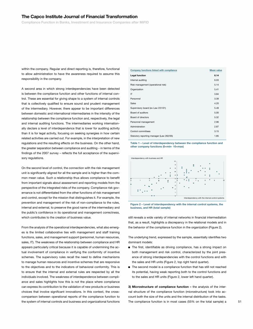
51

The Capco Institute Journal of Financial TransformationCompliance Function in Banks, Investment and Insurance Companies after MiFID

within the company. Regular and direct reporting is, therefore, functional

to allow administration to have the awareness required to assume this

responsibility in the company.

A second area in which strong interdependencies have been detected

is between the compliance function and other functions of internal con-

trol. These are essential for giving shape to a system of internal controls

that is collectively qualified to ensure sound and prudent management

of the intermediary. However, there appear to be important differences

between domestic and international intermediaries in the intensity of the

relationship between the compliance function and, respectively, the legal

and internal auditing functions. The intermediaries working internation-

ally declare a level of interdependence that is lower for auditing activity

than it is for legal activity, focusing on seeking synergies in how certain

related activities are carried out. For example, in the interpretation of new

regulations and the resulting effects on the business. On the other hand,

the greater separation between compliance and auditing – in terms of the

findings of the 2007 survey – reflects the full acceptance of the supervi-

sory regulations.

On the second level of control, the connection with the risk management

unit is significantly aligned for all the sample and is higher than the com-

mon mean value. Such a relationship thus allows compliance to benefit

from important signals about assessment and reporting models from the

perspective of the integrated risks of the company. Compliance risk gov-

ernance is not differentiated from the other functions of risk management

and control, except for the mission that distinguishes it. For example, the

prevention and management of the risk of non-compliance to the rules,

internal and external, to preserve the good name of the intermediary and

the public’s confidence in its operational and management correctness,

which contributes to the creation of business value.

From the analysis of the operational interdependencies, what also emerg-

es is the limited collaborative ties with management and staff training

functions, sales, and management support (personnel, human resources,

sales, IT). The weakness of the relationship between compliance and HR

appears particularly critical because it is capable of undermining the ac-

tual involvement of compliance in verifying the conformity of incentive

schemes. The supervisory rules recall the need to define mechanisms

to manage human resources and incentive schemes that are responsive

to the objectives and to the indicators of behavioral conformity. This is

to ensure that the internal and external rules are respected by all the

individuals involved. The weakness of interdependence between compli-

ance and sales highlights how this is not the place where compliance

can express its contribution to the validation of new products or business

choices that involve significant innovations. In this context, the cross-

comparison between operational reports of the compliance function to

the system of internal controls and business and organizational functions

still reveals a wide variety of internal networks in financial intermediation

that, as a result, highlights a discrepancy in the relational models and in

the behavior of the compliance function in the organization (Figure 2).

The underlying trend, expressed by the sample, essentially identifies two

dominant models:

■■ The first, identifiable as driving compliance, has a strong impact on

both management and risk control, characterized by the joint pres-

ence of strong interdependencies with the control functions and with

the sales and HR units (Figure 2, top right hand quarter).

■■ The second model is a compliance function that has still not reached

its potential, having weak reporting both to the control functions and

to the sales and HR units (Figure 2, lower left hand quarter).

3) Microstructure of compliance function – the analysis of the inter-

nal structure of the compliance function (microstructure) took into ac-

count both the size of the units and the internal distribution of the tasks.

The compliance function is in most cases (55% on the total sample) a

0

1

2

3

4

5

6

7

8

9

10

0 1 2 3 4 5 6 7 8 9 10

Interdependency with business and HR

Interdependency with the internal control systems

Figure 2 – Level of interdependency with the internal control systems, the business, and HR (total sample)

Company functions linked with compliance Mean value

Legal function 6.14

Internal auditing 6.03

Risk management (operational risk) 5.14

Organization 5.41

IT 3.84

Personnel 3.39

Sales 4.20

Supervisory board (ex Law 231/01) 5.49

Board of auditors 5.00

Board of directors 5.32

Personnel management 2.96

Administration 2.87

Control committees 3.15

Statutory reporting manager (Law 262/05) 1.85

Table 1 – Level of interdependency between the compliance function and other company functions (0=min- 10=max)

52

structured and comprehensive unit, equipped with dedicated staff. In

smaller cases, on the other hand, in particular CBs, there are more fre-

quently monocratic solutions, characterized by the sole presence of a

compliance officer who, in certain situations, resorts to outsourced func-

tions. The solution represented by a compliance function that benefits

from staff from other structures within the bank is present in less than

20% of the sample. More than 70% of international intermediaries, gen-

erally represented by large companies, have articulated facilities, com-

pared to those with a purely domestic matrix for which the percentage

falls to 45%. Moving on to the size of the compliance function, one notes

that the average number of employees of the compliance function lies

between one and five full time staff, equivalent to 64% of cases, confirm-

ing the characteristics found in the 2007 survey, but the range is between

0 and 500 full time employees.

4) Planning compliance activities and which resources to use – the ef-

fectiveness of managing compliance risk makes it increasingly important

to carefully plan and program actions and participation in the compliance

function within the company structure, as seen in the preparation of a for-

mal action plan in the majority of cases (91%). The planning activity of the

compliance function should include their management and the efficient

use of any corporate resources allocated to the function. The cases of an

independent budget for the compliance function are more frequent than

in 2007 (46.4% versus 31.4%), although domestically such an allocation

is not yet qualified as a usual procedure as compared to the international

players. This applies in a more marked way to the cooperative banks

than to the other types of intermediaries. As of 2007, the amount of the

budget allocated by all the domestic banks and other intermediaries lies

below €500,000. For foreign banks, where there is a growing business

and organizational complexity and a need to ensure tangible autonomy

and independence in the compliance function, the financial resources are

sometimes at levels higher than the 2007 budget (with 7% of the sample

up to €2 million and 10% of the sample over that amount).

Roles attributed to the compliance functionTo understand the effectiveness of the compliance function it is neces-

sary to consider the resources (human) and the techniques used (the

information systems developed in software, hardware, and communica-

tion networks) to evaluate whether they are appropriate for the foreseen

changes and to assess the trend of costs that their use, and more gener-

ally the execution of the compliance function, entails. Only in this way is

it possible to put some light into the “black box” of this new company

function, helping to stimulate debate – which is already very lively in the

companies – on what to do and on how to do it to create a competitive

advantage element and to not only view it as a “supervisory burden.” In

this part of the study we try to: identify the skill level used in carrying out

the tasks; understand the responsibility of the compliance officer; note

the degree and type of dissemination of IT support for the activities of

the function; and highlight the main factors of change expected from the

function, and estimate the expectations about the related costs for the

next three years.

1) Level of skills and time allocation within the framework of the

compliance function – In this study we note the level of skills of those

currently engaged in the compliance function (their various know-how,

ability, and experience) who were asked to fill in this evaluation. The most

important skills are those covering the regulation framework and the in-

vestment products and services, followed by legal competences, those

relating to the organization, and auditing. Interpretation of the compliance

function using a more traditional view (external regulations) seems to pre-

vail in the broader strategic outlook of compliance business partners. The

knowledge appears homogeneous for all financial intermediaries. This

could emphasize the need for such intermediaries to have similar skills in

the compliance function despite their positioning at different points in the

production-distribution chain.

2) Responsibilities of the compliance function – with reference to the

responsibilities of the compliance officer, various items, listed in Table 2,

were taken into consideration. In general, one notes that from this point

of view the function is defined by a small difference between the average

values which describe its responsibilities and that involves, at the stra-

tegic level, the protection of compliance culture and, at the operational

level, the management of the qualifying processes of its activities. For

82% of the intermediaries (69 in absolute numbers) there is a detailed

description which is formalized by the assigned tasks. The remaining

18% did not reply or do not possess such a description. It is considered

fundamental that there be a formalized description, highlighting in detail

the responsibilities of the function, its links with top management, busi-

ness line and support units, and others working in the system of con-

trols (supervisory organ ex 231/2001, audit, risk management). The total

or partial lack of such a description renders the responsibilities of the

function unclear, and hence the organizational solutions it adopts. This

obviously gives a marked negative value when it comes to judging how

adequate the function is.

3) Distribution of IT supports and resulting investments for the com-

pliance function – compared to the previous edition of the survey, it is

confirmed in principle that the compliance function can draw great ben-

efits from adequate technical resources when faced with a wide range of

activities and involvement, and is characterized by great pervasiveness

within intermediaries and banks. This availability is essential and of grow-

ing importance with the size, degree of diversification, and spatial breadth

of the intermediary increases. In 2007 a little over half of the sample did

not use dedicated applications. A significantly greater number of interna-

tional intermediaries replied positively than domestic ones. The difference

between banks and other intermediaries was not as strong, but it was

53

always present; it was the latter that used dedicated applications. In this

edition of the survey, eight cases did not reply to the question, while the

remainder is divided between those that have no dedicated technological

applications [48.8% (41 cases)] and those that replied positively [44% (37

cases)]. In situation where there are dedicated applications, the information

on the running of the compliance function is drawn from other information

systems and procedures of the company. The most widely used sources

are autonomous and customized extractions from other information sub-

systems in the company (34 cases), and to a lesser extent from systems

and procedures used for operating risk (19 cases) and from control man-

agement (nine cases). There are no significant differences between the dif-

ferent types of intermediaries, or between domestic and international ones.

One can only note that there is a greater number of insurance companies

and domestic intermediaries use autonomous extractions. What we ob-

served in the 2007 data can also be seen in the current survey, namely the

partial overlap between operational risk management and of the compli-

ance in terms of some events leading to risk and to their monitoring, which

partly justifies their responses.

4) Reason for change and progress expected from the costs of the

compliance function – the answers given in the previous survey showed,

in general, the prevalence of the regulatory factors context, ranking at

the same level the evolution of European and domestic legislation. This

was then followed by a certain distance by the awareness of sanctions

by control units. In fourth place appeared to be the wish to improve the

quality of customer services. The best practice in the sector, the interven-

tions of the Basel Committee, and the technological changes had scores

below average (confirming the scarce inclination of the subject). In the

new survey, on a 1-10 scale of degree of agreement, between the evolu-

tion of domestic legislation (8.85) and the evolution of European legisla-

tion (7.60), commitment of top management (7.79) becomes crucial. The

other answers are in line with evidence from the previous survey (in fourth

place was the resolve to improve the quality of customer services, in fifth

the awareness of sanctions, and so on). In last place is the confirmation

of technological change, once again with limited answers.

In the previous survey, we observed that the expectations of cost growth

were relatively more prevalent in international financial intermediaries

(61%) than in the national (50%) ones. This seemed somewhat surpris-

ing, since compliance capabilities appeared more advanced in interna-

tional intermediaries. In this survey, the cost deceleration appears gener-

alized: the crisis in the sector has led to limiting costs, even though those

for compliance, considering all that has recently occurred, should not

change as drastically as indicated (Figure 3).

Measuring, transferring, and mitigating compliance risk in the investment industryWe take an in-depth look at the degree of development of the compli-

ance risk management process, namely those phases that enable the

measurement and, consequently, active management of the positions at

risk. In particular, we studied the measuring process and the mitigation

solutions.

1) Measurement of compliance risk – the 2007 survey showed that

only 42% of the respondents completed the qualitative/quantitative

phase of the measuring process, while in 2009 that percentage had risen

to 46.8%, proving that there was increasing adherence to regulatory con-

straints. What has markedly changed is the spread found when com-

paring intermediaries, in particular those who mainly cover the domestic

sector, as compared to those involved in international activities or direct

foreign governance. In the 2007 survey 26.3% of domestic firms used a

metric for compliance, in 2009 that percentage had risen to 44.9%. The

widening of the sample, compared to 2007, results in a rebalance for the

intermediaries covering foreign areas. For the international subsample,

the percentage of firms capable of measuring risk went from 66.7% to

50%. Evidence for the 2007 results comes from the segmentation of in-

termediaries: in 2007, banks and other financial intermediaries exhibited

a different behavior. In 2009, the evidence shows how the approaches

were more homogeneous. The main difference is between insurance

companies and cooperative banks (CBs): the latter show a lower value

Responsibilities Mean value

Strong involvement in the daily activities 7.28

Presiding links to the supervisory authority 7.67

Ensuring that the compliance culture is present top-down within

the company

8.41

Developing the regulatory infrastructure of the group/each single

intermediary

7.00

Consulting and guiding on regulatory matters 8.05

Implementing the compliance infrastructure 7.90

Evaluating whether the compliance function is adequate and appropriate 6.56

Table 2 – Responsibilities of the compliance Officer (from 0 = min to 10 = max)

2.9%

34.3%

20.0% 20.0%

11.4%

0.0% 2.6%

15.4%

38.5%

43.6%

0%

10%

20%

30%

40%

50%

Stable Substantial increase Slight increase Slight decrease Substantial decrease

Total 2007

Total 2009

Figure 3 – Expectations about the costs of compliance in the next three years (2007 versus 2009, relative frequencies)


54

compared to the whole sample. This depends on the complexity of the

CBs, which frequently choose a network solution to minimize costs.

2) Mitigation tools for the compliance risk – there is a difference be-

tween the domestic and international areas of activity by mitigation solu-

tions. If we consider the no-replies as a lack of specific tools used to man-

age risk, only 9% of the domestic candidates apply instruments aimed at

limiting risk. This increased to 28% for the international sector. Overall,

only 15.5% implemented tools to manage the compliance risk; the ma-

jority (62%) used insurance tools. This is a major difference with the 2007

survey, when no firms used to transfer the risk. A significant number of

firms introduced codes of conduct to minimize the compliance risk prob-

ability. Only in banks were there cases where the code of conduct was

not implemented. The use of a specific code of conduct by business lines

shows they are associated with the negotiation of financial instruments,

defined as trading and sales; this is followed by asset management and

investment banking. There are no significant differences between the in-

ternational and domestic institutions except for retail banking, where no

positive responses were provided by the former group.

Compliance function’s interaction inside and outside the structureThe compliance function’s interactions both internally and externally are

examined in four areas:

1) The internal and external communication instruments used by the

compliance function.

2) The contribution to innovation processes that affect the area of in-

vestment services.

3) The connecting mechanisms and processes between the compli-

ance function and the system of corporate values and between the

compliance function and the incentive system.

4) The involvement of the compliance function during the implementa-

tion phase of the MiFID Directive.

1) Internal and external communication tools – in the regulatory frame-

work, the compliance function is defined as a second level control func-

tion. Consequently, it is essential to communicate both within the struc-

ture of the intermediary and outside, through communication processes

that encourage a dialogue between the institutional players and the pro-

cess that disseminates the company values to the public.

As can be seen in Table 3, a high level of importance is allocated by the

compliance function to Internet and email, as forms of communication

that are both capillary and less expensive, through which a wide range

of information can be sent to all the levels of the company. Meetings are

also allocated relatively high values. Meetings are an instrument of com-

munication for small groups of people, with high relational content, but

costly in terms of time and personnel. It is, therefore, plausible that these

are used in particular by the larger intermediaries and above all during the

initial phase when preparing company policies. The use of circulars, as a

means of spreading the common interpretation of hetero- and self-regu-

lation clearly and unequivocally, is especially appreciated by banks and

other financial intermediaries, while it is not as widely used by insurance

companies. Moreover, the communication of compliance values through

the internal code and training courses carried out mainly by international

intermediaries is, in fact, less crucial for domestic intermediaries. Link-

ing this last point with what was said concerning the responsibilities of

the compliance officer indicates an element of inconsistency, between

the willingness to make the culture of conformity and the use of internal

communication instruments. In Table 2 the mean value attributed to “en-

sure that the culture of compliance be present top-down” is 8.41, on a

scale from 0 to 10. With this indication one could expect that, even dur-

ing the application of internal communication tools, it was sustained by

dedicated training courses or, at least, by a widespread circulation of the

internal code stressing this point.

For external communication tools, the survey considered the elements

identified in Table 4. The instruments with greater external visibility, such

as the documents on the website and the use of codes of conduct, are

more widely used by international intermediaries. Domestic firms indi-

cated that they tend to use financial statements and congress participa-

tion for communication.

Internal communication tools Mean value

Intranet and email 8.44

Meetings 7.51

Participation in training courses 4.25

Dedicated training courses 4.31

Internal codes 4.65

Circulars 5.68

Report to administration 7.38

Report to internal audit 5.08

Table 3 – Internal communication tools (importance 0 min -10 max)

External communication tools Mean value

Annual report 3.62

Social balance sheet 3.29

Code of conduct 3.43

Documents on the website 4.33

Conference participation 3.45

Table 4 – External communication tools (importance 0 = min - 10=max)

55

In particular, with reference to the annual report, 30% of respondents,

regardless of the type of membership, gave it a communication value

of zero on a scale from 0 to 10. It is important to think about this figure

on which the annual report is based, and the type of instrument used to

transmit a message of reputation and cultural integrity to the public and

to the supervisory authorities.

2) Contribution of the compliance function to the innovative proc-

esses – the compliance function, through the spreading of a common

culture aimed at respecting the rules and the dialogue between the vari-

ous company functions can contribute to improving opportunities for

innovation in investment services. The design of new products or the

creation of processes to improve the operating conditions within the in-

termediaries in acting according to the rules of the game can become

strategic when it comes to enhancing the reputation and capturing of

new market shares. From the empirical survey one notes that 76% of

the domestic intermediaries and 78% of the international ones consider

that the compliance function could have a driving role in the innovative

processes on the stipulation of investment services. In banks mainly op-

erating domestically, as already pointed out in the previous survey, the

proximity of the compliance function to other business functions involved

in the processes of products/services production could facilitate the dia-

lectic exchange and support the comparison.

3) Link between the compliance function, the system of corporate

values, and the incentive system – for companies subject to regula-

tion, the search for innovative solutions may not lead to working outside

the external and internal rules of the game. The sensitivity of this aspect

came to light internationally during the last financial crisis: the trustee

in the allocation of resources between investors and borrowers needs

the highest level of protection to avoid the systemic risk of crisis trans-

mission by the financial sector to the rest of the economy. Compliance

with the rules must be in the DNA of the financial intermediaries who are

subject to regulation since they are allowed to operate for savers who

contribute their savings and the subsequent choice of investment leading

to the development of the economic system.

This statement implies on the one hand, visibility, when the compliance

function finds it fits the value system of the corporation and, on the other

hand, concreteness, when in the company there are operational mecha-

nisms or processes that connect the principle of conformity to the ex-

ternal and internal rules with the incentive system. The survey notes the

presence or absence of such connections and suggests the following

combinations (Figure 4):

■■ Absence of a link with the system of values and incentives (no; no).

■■ Presence of a link with the system of values, absence of a connection

with incentives (yes, no).

■■ Absence of a link with the system of values, presence of a connection

with incentives (no; yes).

■■ Presence of a link with the system of values and incentives (yes; yes).

As in the previous survey, in the current study the “virtuous” situation of

the presence of a connection to both the levels of system of values and

incentives also characterizes the minority of those interviewed 11.6% of

cases. At the other extreme, the absence of both links is recognized in

40.6% of the sample (this was 28.6% in 2007). In 27.5% of the cases, the

link is present at the level of system values, but not for incentives, while

for only 4.3% the situation was the opposite, i.e., the link is exclusively

present at the incentive level. With regard to the connection between the

values of compliance and the incentive system, when present it is mainly

represented (in 68% of cases) by the use of evaluation processes through

subjective procedures. In a minority of cases, objective procedures are

given where indicators of conformity in the individual incentive system

are used.

4) Level of involvement of the compliance function in complying with

the MiFID Directive – this survey aims to explicitly observe the involve-

ment of the compliance function in internal processes of corporate ad-

justment to the MiFID Directive, taking into account its current Level 3

stage. The results prove that the compliance function is mainly seen as

having a driving and advisory role, being less relevant during the imple-

mentation phase: 52.4% of those interviewed pointed to the advisory

role, which reflects the intrinsic planning part of the function, while 47.6%

pointed to its thrusting power, 14.3% reported on its role of accomplisher

(compared to 2007, what is changing is the perception between its roles

as a driving force and as an advisory service, in the present phase the

latter prevails). The thrust is especially present in the compliance func-

tion of international intermediaries. For domestic firms what is preferred

is its internal advisory approach. On this point, there is probably also a

learning curve of the potential, inherent to the role of the compliance

function, which some domestic intermediaries still have to master. There

were also significant differences of interpretation between the types of

28.57% 25.71%

8.57%

20.00% 17.14%

40.58%

27.54%

4.35%

11.59%

15.94%

0%

5%

10%

15%

20%

25%

30%

35%

40%

45%

No;No Yes;No No;Yes Yes;Yes (vuoto)

Total 2007 Total 2009

Figure 4 – Connection between compliance function – value system – incentive system (2007 versus 2009, relative frequencies)


56

intermediaries, where the most striking was between banks and insur-

ance companies, but also between banks and other financial intermedi-

aries and within the bank sector. For banks, the compliance function is

seen as the driving force and advisor, covering the broad majority of the

sample (over 60%). Only a minority of insurance companies considered

these two properties important, confirming the recent history of the com-

pliance function in this sector. Finally, always with reference to the type

of intermediaries, the other financial intermediaries and the smaller sized

banks considered the advisory role most significant while that of being a

driving force was only noted by a few of the smaller banks.

ConclusionThis study focuses on the evolving scenario of the compliance func-

tion within banks, investment firms and insurance companies during the

implementation of the MiFID Directive. Focusing on the positioning of

the compliance function, almost half of those who were interviewed are

reporting to the boards of directors. Alternative solutions are still on the

way and the link to the top is through the general director or the CEO as

mediators. Regarding the responsibilities and the roles assigned to the

compliance function, from a strategic point of view, the function itself feels

the need for the culture to be more compliance-focused and that there

should be, at a working level, qualifying management procedures for the

activity itself. A significantly higher number of financial players have im-

plemented qualitative/quantitative methods to measure the risk and have

started to transfer the impact using insurance contracts. Regarding the

interaction in/out of the structure, the vast majority of domestic and inter-

national intermediaries believe that the compliance function could carry

out an active role for innovative processes in investment services, but

only a minority of the sample shows a virtuous situation of a connection

between the value system and the compliance principles and the internal

incentive system. With regard to the role of the compliance function in

the implementation of the MiFID Directive, the results reflect the net inter-

pretation of the role mainly as pushing (initiator) and consulting (advisor)

of the compliance function and less relevant during the implementation

phase (actor). The innovative effort is very strong in the compliance func-

tion of the international players, while the domestic players prefer the

internal consulting approach. This is probably because there is a learning

curve of the intrinsic potentials of the role of the compliance function that

still has to be carried out by some domestic intermediaries.

References• Bank of Italy – CONSOB, 2007, “Regolamento in materia di organizzazione e procedure

degli intermediari che prestano servizi di investimento o di gestione collettiva del risparmio,”

www.consob.it

• Bank of Italy, 2006, Supervisory legislation for conformity regulations (compliance), Reference

Document, www.bancaditalia.it

• Bank of Italy, 2007, Disposizioni di vigilanza, La funzione di conformità (compliance),”

www.bancaditalia.it

• Basel Committee on Banking Supervision, 2005, “Compliance and the compliance function in

Banks,” April

• Basel Committee on Banking Supervision, 2008, “Implementation of compliance principles,”

August

• CE 2004/39/CE, www.consob.it

• CE 2006/73/CE, www.consob.it

• CEIOPS, 2008, “Implementing measures on system of governance,” November, www.ceiops.

org

• Gabbi G., P. Musile Tanzi, and L. Nadotti, 2011, “Firm size and compliance costs asymmetries

in the investment services,” Journal of Financial Regulation and Compliance, forthcoming

• ISVAP, 2008, Regolamento n. 20 del 26 marzo 2008, www.isvap.it

• Musile Tanzi P., G. Gabbi, P. Schwizer, D. Previati, and M. Poli, 2008, “Compliance risk in the

evolution of investment services,” SDA Bocconi Working Paper, January, http://ssrn.com, 1-150

• Musile Tanzi, P., A. Alberici, G. Gabbi, M. Gallo, L. Nadotti, R. Pisani, M. Poli, D. A. Previati,

A. Schwizer, V. Stefanelli, and R. T. Colonel, 2009, “The evolution of compliance function and

compliance risk in investment services,” SDA Bocconi Working Paper, June, http://ssrn.com,

1- 191

57

PART 1

Investor Irrationality and Closed-end Hedge Funds

AbstractThe present study assesses the rationality of investors who

pay large sums to hedge fund managers for their services.

For my analysis I use a sample of closed-end funds which

invest their capital in one or more open-ended hedge funds.

The results imply that investors rationally exploit the avail-

able information when deciding whether to engage in the

initial public offering of a new closed-end fund. However, I

also find evidence that investors react with a burst of irratio-

nal pessimism to the worsening economic conditions in the

second half of 2008.

Oliver Dietiker — Research Assistant, University of Basel

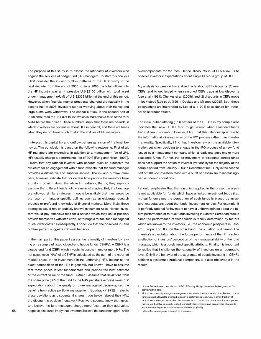
58

The purpose of this study is to assess the rationality of investors who

engage the services of hedge fund (HF) managers. To start this analysis

I first consider the in- and outflow patterns of the HF industry in the

past decade: from the end of 2000 to June 2008 the total inflows into

the HF industry was an impressive U.S.$2100 billion with total asset

under management (AUM) of U.S.$2339 billion at the end of this period.

However, when financial market prospects changed dramatically in the

second half of 2008, investors started worrying about their money and

large sums were withdrawn. The capital outflow in the second half of

2008 amounted to U.S.$821 billion which is more than a third of the total

AUM before the crisis.1 These numbers imply that there are periods in

which investors are optimistic about HFs in general, and there are times

when they do not have much trust in the abilities of HF managers.

I interpret this capital in- and outflow pattern as a sign of irrational be-

havior. This conclusion is based on the following reasoning. First of all,

HF managers are expensive: in addition to a management fee of 2%,

HFs usually charge a performance fee of 20% [Fung and Hsieh (1999)].

I claim that any rational investor who accepts such an extensive fee

structure for an engagement with a fund expects that the fund manager

provides a distinctive and superior service. The in- and outflow num-

bers, however, indicate that for certain time periods the investors have

a uniform opinion about the whole HF industry; that is, they implicitly

assume that different funds follow similar strategies. But, if all manag-

ers followed similar strategies, it would be unlikely that they would be

the result of manager specific abilities such as an elaborate research

process or profound knowledge of financial markets. More likely, these

strategies would rely on publicly known investment rules. Hence, inves-

tors would pay extensive fees for a service which they could possibly

provide themselves with little effort, or through a mutual fund manager at

much lower costs.2 Consequently, I conclude that the observed in- and

outflow pattern suggests irrational behavior.

In the main part of this paper I assess the rationality of investors by rely-

ing on a sample of listed closed-end hedge funds (CEHFs). A CEHF is a

closed-end fund (CEF) which invests its assets in one or more HFs. The

net asset value (NAV) of a CEHF is calculated as the sum of the reported

market prices of the investments in the underlying HFs. Insofar as the

exact composition of the HFs is generally not known I have to assume

that these prices reflect fundamentals and provide the best estimate

of the current value of the fund. Further, I assume that deviations from

the share price (SP) of the fund to the NAV per share express investors’

expectations about the quality of future managerial decisions, i.e., the

benefits from active portfolio management [Boudraux (1973)]. I refer to

these deviations as discounts; if shares trade below (above) their NAV,

the discount is positive (negative).3 Positive discounts imply that inves-

tors believe the fund managers charge more fees than they add value,

negative discounts imply that investors believe the fund managers’ skills

overcompensate for the fees. Hence, discounts in CEHFs allow us to

observe investors’ expectations about single HFs or a group of HFs.

My analysis focuses on two stylized facts about CEF discounts: (1) new

CEFs tend to get issued when seasoned CEFs trade at low discounts

[Lee et al. (1991); Cherkes et al. (2005)], and (2) discounts in CEFs move

in lock-steps [Lee et al. (1991); Doukas and Milanos (2005)]. Both these

observations are interpreted by Lee et al. (1991) as evidence for irratio-

nal noise trader effects.

The initial public offering (IPO) pattern of the CEHFs in my sample also

indicates that new CEHFs tend to get issued when seasoned funds

trade at low discounts. However, I find that this relationship is due to

the informational idiosyncrasies of the IPO process rather than investor

irrationality. Specifically, I find that investors rely on the available infor-

mation set when deciding to engage in the IPO process of a new fund

issued by a management company which already manages one or more

seasoned funds. Further, the co-movement of discounts across funds

does not support the notion of investor irrationality for the majority of the

sample period from January 2003 to December 2008. Only in the second

half of 2008 do investors react with a burst of pessimism to increasingly

bad economic conditions.

I should emphasize that the reasoning applied in the present analysis

is not applicable for funds which have a limited investment focus (i.e.,

mutual funds) since the perception of such funds is biased by inves-

tors’ expectations about the funds’ investment ranges. For example, it

is perfectly rational for investors to have a uniform opinion about the fu-

ture performance of mutual funds investing in Eastern European stocks

since the performance of these funds is mainly determined by factors

which are known to the investors, i.e., the economic prospects in East-

ern Europe. For HFs, on the other hand, the situation is different. The

investor’s expectation about the future performance of the HF is solely

a reflection of investors’ perception of the managerial ability of the fund

manager, which is a purely fund specific attribute. Finally, it is important

to realize that I challenge the rationality of investors on an aggregate

level. Only if the behavior of the aggregate of people investing in CEHFs

exhibits a systematic irrational component, it is also observable in the

results.

1 I thank Sol Waksman, founder and CEO of Barclay Hedge (www.barclayhedge.com), for

providing this data.

2 Mutual funds usually charge a management fee which does not exceed 1%. Further, mutual

funds are not allowed to charged excessive performance fees. Only a small fraction of

mutual funds charges a so-called fulcrum fee, which has similar characteristics as a perfor-

mance fee, but that is closely related to industry benchmarks and can only be charged to

institutional or high-net worth investors [Elton et al. (2003)].

3 I also refer to a negative discount as a premium.

59

Relation to other studiesThe present paper is motivated by two streams of literature that try to ex-

plain the often puzzling patterns in discounts of CEFs.4 The first stream is

pioneered by Lee et al. (1991) which interpret fluctuations in discounts of

CEFs as a symptom of irrational investor behavior. A countermovement

initiated by Ross (2002a, b) relies on the reasoning of neoclassical finance

and refuses to accept irrationality as the primary argument. These latter

studies re-adopt several ideas first discussed in Malkiel (1977).5 I empha-

size that my study does not intend to provide new explanations for the CEF

puzzle but rather to examine whether investors exhibit irrational behavior.

The study of Lee et al. (1991) is based on the noise trader model introduced

in DeLong et al. (1990). In this model discounts are driven by irrational

investors who commonly react to unqualified information (noise) and ran-

domly drive prices of CEF below and above their NAV. Rational investors

who want to exploit their superior beliefs have to account for the possibility

Name List date Market 2008 Average discount Discount 2008 Type

Alternative Investment Strategies Dec-96 197.4 3.80% 27.40% MMF

HSBC European Absolute* 04-Jan 19.0* 1.6%* 1.3%* MMF

Dexion Absolute 12-Feb 838.1 -1.70% 31.70% MMF

Thames River Hedge 02-Apr 211.4 -0.20% 39.90% MMF

Dexion Equity Alternative 04-Apr 99.7 2.10% 18.60% MMF

Dexion Trading 11-Apr 108.6 1.60% 21.00% SMF

HSBC Global Absolute 11-Apr 84.3 2.20% 33.40% MMF

Absolute Return trust 01-May 202 -1.10% 23.30% MMF

Acencia Debt Strategies 02-May 99.3 -0.50% 40.00% MMF

Tapestry Investment Company 02-May 52.5 2.10% 36.00% MMF

RAB Special Situations 05-May 15.7 16.40% 55.40% SMF

KGR Absolute Return 11-May 50.7 1.60% 18.00% MMF

Value Catalyst Fund 12-May 94.3 -1.80% -4.70% SMF

The Cayenne Trust 01-Jun 29.8 2.00% 4.40% SMF

BlueCrest All Blue 05-Jun 241.8 2.50% 17.10% SMF

CMA Global Hedge 07-Jun 111.3 5.00% 56.80% MMF

Goldman Sachs Dynamic Oppt. 07-Jun 214.4 4.70% 43.30% MMF

New Star Abs. Ret. Growth** 08-Jun 20.2** 1.8%** 3.9%** SMF

New Star Abs. Ret. Value** 08-Jun 18.2** 1.0%** 2.9%** SMF

Cazenove Absolute Equity 10-Jun 62.8 -0.30% 17.40% SMF

New Star HDGE 250 Index 1x 11-Jun 52.7 1.50% 20.10% MMF

New Star HDGE 250 Index 3x 11-Jun 2.4 3.60% 51.70% MMF

Signet Global Fixed Strategies 11-Jun 35 -0.40% 26.30% MMF

Invesco Perpetual Select Hedge 11-Jun 19.5 1.20% 2.80% MMF

Aida Fund 12-Jun 24.1 2.40% 13.10% MMF

Dexion Alpha Strategies 03-Jul 60.7 5.50% 34.20% MMF

FRM Credit Alpha 03-Jul 56 1.00% 27.20% MMF

BH Macro 03-Jul 942.4 -1.00% 17.40% SMF

Gottex Market Neutral 03-Jul 25.3 3.50% 31.60% MMF

JP Morgan Progressive 05-Jul 17.2 -1.10% 11.20% SMF

F&C Event Driven*** 06-Jul 37.7 8.70% 29.90% MMF

Saltus European Debt Strategies 06-Jul 16.6 7.10% 35.30% MMF

Third Point Offshore 08-Jul 123.8 11.60% 43.80% SMF

Terra Catalyst 02-Aug 38.5 9.90% 41.30% SMF

Black Rock Absolute Return 04-Aug 71.4 3.00% 42.90% MMF

BH Global 05-Aug 462.2 5.50% 28.00% SMF

FRM Diversified Alpha 06-Aug 34 20.00% 32.80% MMF

*delisted in 09/08; **delisted in 07/08. ***delisted in 01/09

The listing date (‘list date’) denotes the month in which shares of the fund start trading on the London Stock Exchange. Three funds are delisted before the end of 2008. The market volume (Market

2008) is denoted in euro millions and taken at the last trading day of 2008 (or the month before delisting). The figure denotes the sum of the market volume of all share classes. The discount for

month is calculated as where NAV is the month-end net asset value of the fund, and where SP is the month-end share price. The average discount (Average discount) denotes the average of the

month-end discounts from inception of the fund to the end of 2008 (or to its delisting). The discount for the end of 2008 (or the last month before delisting) is denoted as “Discount 2008”. If a share

is traded in more than one currency class, I use the share class with the largest market capitalization. The last column (type) denotes whether the CEHF is incorporated as a single manager fund

(SMF) or as a multi manager fund (MMF).

Table 1 – Closed-end hedge funds listed on the London Stock Exchange

The Capco Institute Journal of Financial TransformationInvestor Irrationality and Closed-end Hedge Funds

4 These puzzling fluctuations are usually summarized as the CEF puzzle [Lee et al. (1990)].

5 I do not consider the effect of market frictions but refer to Pontiff (1996) for a study on the

influence of arbitrage costs and to Datar (2001) and Cherkes et al. (2005) for a discussion

on the impact of liquidity.

60

that their irrational counterparts take even more extreme positions during

their investment period. As a consequence, prices are not fully driven back

to the NAV in equilibrium and usually trade below their NAV due to the

additional risk introduced by noise traders. Lee et al. (1991) refer to these

collective bursts of optimism or pessimism as investor sentiment.6 Two

implications of the noise trader model are relevant for my study: funds tend

to get started when seasoned funds trade below their NAVs and discounts

of seasoned funds move together. The second stream of related literature

initially proposed by Ross (2002a, b) explains changes in discounts based

on agency costs. These studies usually explain how funds get issued at

a premium and then move into discounts.7 However, none of these stud-

ies manages to explain the comovement in discounts which is reported

in several studies [Bodhurta et al. (1995), Pontiff (1997) and Doukas and

Milanos (2004)]. Hence, comovement in discounts across funds is a strong

argument favoring irrational investor behavior.8

Description of the sample and variable definitionThe sample for the main analysis of this study consists of 37 CEHFs

that have been admitted to trade on the London Stock Exchange (LSE)

between 1996 to 2008 (Table 1). I do not consider funds that have been

admitted to other markets prior to being listed on the LSE.9 Information

on the funds is gathered from several sources: the annual reports are

the primary source for information on the manager of the fund and the

issuance of new shares; the monthly newsletters provide month-end net

asset values (NAVs) per share; data on month-end shares prices and

market capitalization are obtained from Datastream. CEHFs can be di-

vided into two categories: single manager funds (SMFs) and multi man-

ager funds (MMFs). A SMF is a CEF that invests its assets according to

the advice of a single HF manager. The SMFs usually act as feeder funds

for seasoned, unlisted HFs. A MMF is a CEF that exhibits a fund of HFs

structure. The manager of the MMF chooses to invest the fund’s assets

in several HFs that he or she expects to provide superior performance.

Hence, the performance of a MMF depends on the ability of several HF

managers. The MMFs outnumber the SMFs both in number and market

capitalization. By the end of 2009, the 24 listed MMFs had a market capi-

talization of €3,594.11 million, the 13 SMFs had a market capitalization

of €1,212.89 million.

The difference between the SMFs and the MMFs is best observable in the

fee structure. Investments in the MMFs are subject to two layers of fees.

The managers of the MMFs charge management and performance fees

for selecting other fund managers. Additionally, the selected HF manag-

ers charge management and performance fees for their services. In my

sample the managers of the MMFs charge, on average, 1.3% manage-

ment fee and 11.2% performance fee. The SMFs charge only one layer

of (significant) fees. While the investment in the master fund is subject to

management and performance fees, at the level of the SMF a (compa-

rably) small administration fee is charged. Several CEHFs are offered in

more than one currency class. The most common currency classes are

U.S.$, euro, and pound sterling (GBP). Each currency class has a sepa-

rate account and costs are allocated to these accounts. Moreover, each

class has its own international security identification number and is indi-

vidually traded. For each fund I only consider the class that exhibits the

highest market capitalization since this class is usually the most liquid.

I express the discount of the asset at the end of month as disci,t = (NAVi,t

– SPi,t)/NAVi,t, where NAVi,t and SPi,t are the month-end NAV and month-

end share price of fund i for month t. Note that discounts are positive

if the fund’s shares trade below its NAV per share. Following Lee et al.

(1991), I construct a value weighted discount (VWD) index: VWDt = Snti=t

wi,t x disci,t, where nt is the number of funds at the end of month t and

wi,t is the weight of fund i at the end of month t. The weight is calculated

using the month-end market capitalization (in euro) of the fund divided

by the total market capitalization of all funds trading at the time. Monthly

changes in VWD are denoted by ΔVWDt = VWDt – VWDt-1.

Similarly, I construct indexes only considering either the SMFs (VWDS)

and or the MMFs (VWDM).

The VWD reflects the average value-weighted discounts of all closed-end

hedge funds trading on the LSE. The average (median) values of VWD is

0.0037 (-0.0068). The discounts strongly increase in the second half-year

of 2008 to a maximum discount of 27%.

I calculate the values of the VWD for the period January 2005 to Decem-

ber 2008. For this period the VWD contains at least seven constituents.

Its values are depicted in Figure 1. Note that for about half the time the

values of the VWD are negative and for the majority of time below 5%

until peaking to almost 27% at the end of 2008. The average (median)

of the VWD is 0.37% (-0.68%). These values are significantly lower than

the values reported in other studies. For example, Lee et al. (1991) report

that the average discount for U.S. funds was around 10% for the period

1965 to 1989, Anderson et al. (2002) report that the average discount in

February 2001 is 10.9% for all equity funds.

6 Lee et al. (1991) argue that investor sentiment presents a new pricing factor for assets gen-

erally held by small investors. This assertion triggered a series of papers such as Chen et

al. (1993), Chopra et al. (1993), Brauer (1993), and Elton et al. (1998).

7 Weiss (1989) reports that funds usually move into discounts within 120 days. Studies

explaining such behavior are Arora et al. (2003) and Ferguson and Leitstikow (2004).

Additionally, the model presented in Berk and Stanton (2007) predicts the wide variation in

discounts across funds by relying on managerial ability and the implications of a long-term

labor contract.

8 To my knowledge Cherkes et al. (2005) is the only study which can explain this behavior

without having to rely on investor irrationality.

9 The names of these funds are obtained from the analyst report on listed hedge funds by

Tom Skinner, Cazenove.

61

Next, I compare the SMFs and MMFs for the period from July 2007 to De-

cember 2008. It is not possible to compare these two indexes for longer

intervals as the SMFs tend to get issued at later times. For the consid-

ered period the SMF contains at least five funds, the MMFs contains at

least 20 funds. The mean (median) discount is 5.49% (4.43%) for VWDS

and 2.52% (-0.02%) for VWDM. These values are significantly different at

the 1% level (two sided test). The lower levels of discounts for the multi

manager funds suggest that investors believe that managers of MMFs

add more value in selecting the funds than they charge for it. Considering

the expensive fee structure of MMFs this result is remarkable. It indicates

that investors are aware that identifying managerial ability is a difficult

task, and they are willing to pay large fees to professionals for providing

this service.

Raising new capitalIn this section I assess whether raising new capital suggests irrational be-

havior as claimed in Lee et al. (1991). I first consider the launching of new

funds, then I focus on the issuance of new capital by seasoned funds.

Launch of new fundsLee et al. (1991) find that new funds tend to get launched when existing

funds trade at a negative discount. They interpret this finding as evidence

for the noise trader model, i.e., it is the result of irrational investor be-

havior. Specifically, they argue that fund managers exploit investors’ ir-

rational optimism by bundling assets together with new funds and selling

them to an appreciative clientele. Nonetheless, Lee et al. (1991) have to

admit that new funds also get started when existing funds trade at a dis-

count – a clear contradiction to the predictions of their model. I observe

a similar pattern (Figure 2): funds tend to get launched after seasoned

funds have traded at low discounts, but I also find that when discounts

are positive managers also raise capital for new funds.

Note that in 2008 four new funds were launched just after the VWD had

risen to a positive level. These four IPOs raised more than €1 billion. I claim

that the observed pattern is not the result of irrational behavior but based

on lack of information. For most investors the amount of information prior

to the IPO of a fund is restricted to what is given in the prospectus. The

prospectus is a legal document that provides a potential investor with in-

formation about a new fund. Its content is specified by the authorities. The

prospectus usually contains (among other information) the legal incorpora-

tion of the fund, the fee structure, the potential risks of such an investment,

and the CVs of the managers. Therefore, it is a valuable tool to enhance

transparency of fund investments. Nonetheless, the information contained

in the prospectus usually does not considerably differ across funds, and it

does not enable the investor to distinguish the specific qualities of a new


-0.1

-0.05

0

0.05

0.1

0.15

0.2

0.25

0.3

01

/01

/20

05

01

/04

/20

05

01

/07

/20

05

01

/10

/20

05

01

/01

/20

06

01

/04

/20

06

01

/07

/20

06

01

/10

/20

06

01

/01

/20

07

01

/04

/20

07

01

/07

/20

07

01

/10

/20

07

01

/01

/20

08

01

/04

/20

08

01

/07

/20

08

01

/10

/20

08

Figure 1 – Month-end values of the VWD from January 2005 to DecemberThe VWD reflects the average value-weighted discounts of all closed-end hedge funds

trading on the LSE. The average (median) values of VWD is 0.0037 (-0.0068). The discounts

strongly increase in the second half-year of 2008 to a maximum discount of 27%.

H1/05 H2/05 H1/06 H2/06 H1/07 H2/07 H1/08 H2/080

1

2

3

4

5

6

7

8

9

10

11

12

nr ip

o

−0.04

−0.03

−0.02

−0.01

0

0.01

0.02

dis

coun

t in

pre

ced

ing

per

iod

H1/05 H2/05 H1/06 H2/06 H1/07 H2/07 H1/08 H2/080

100

200

300

400

500

600

700

800

900

1000

1100

1200

ipo

volu

me

in E

UR

mill

ion

−0.04

−0.03

−0.02

−0.01

0

0.01

0.02

dis

coun

t in

pre

ced

ing

per

iod

H1/05 H2/05 H1/06 H2/06 H1/07 H2/07 H1/08 H2/080

1

2

3

4

5

6

7

8

9

10

11

12

nr is

sue

−0.04

−0.03

−0.02

−0.01

0

0.01

0.02

dis

coun

t in

pre

ced

ing

per

iod

H1/05 H2/05 H1/06 H2/06 H1/07 H2/07 H1/08 H2/080

100

200

300

400

500

600

700

800

900

1000

1100

1200

issu

e vo

lum

e in

EU

R m

illio

n

−0.04

−0.03

−0.02

−0.01

0

0.01

0.02

dis

coun

t in

pre

ced

ing

per

iod

H1/05 H2/05 H1/06 H2/06 H1/07 H2/07 H1/08 H2/080

1

2

3

4

5

6

7

8

9

10

11

12

nr ip

o

−0.04

−0.03

−0.02

−0.01

0

0.01

0.02

dis

coun

t in

pre

ced

ing

per

iod

H1/05 H2/05 H1/06 H2/06 H1/07 H2/07 H1/08 H2/080

100

200

300

400

500

600

700

800

900

1000

1100

1200

ipo

volu

me

in E

UR

mill

ion

−0.04

−0.03

−0.02

−0.01

0

0.01

0.02

dis

coun

t in

pre

ced

ing

per

iod

H1/05 H2/05 H1/06 H2/06 H1/07 H2/07 H1/08 H2/080

1

2

3

4

5

6

7

8

9

10

11

12

nr is

sue

−0.04

−0.03

−0.02

−0.01

0

0.01

0.02

dis

coun

t in

pre

ced

ing

per

iod

H1/05 H2/05 H1/06 H2/06 H1/07 H2/07 H1/08 H2/080

100

200

300

400

500

600

700

800

900

1000

1100

1200

issu

e vo

lum

e in

EU

R m

illio

n

−0.04

−0.03

−0.02

−0.01

0

0.01

0.02

dis

coun

t in

pre

ced

ing

per

iod

Figure 2 – Number of new fund starts in relation to preceding average discounts.

62

fund from the seasoned funds. As a consequence, investors use the avail-

able information about the seasoned funds as a proxy for what to expect

from the new fund, and, therefore, new funds tend to get issued when

investors are optimistic about the existing funds. Hence, it is premature to

conclude that investors are irrational as there is only little information avail-

able on which investors can rationally base their decisions.

I continue the discussion by using a subsample (S1) of 10 funds that are

issued by management companies which are also responsible for the

management of seasoned CEHFs (Table 2). For the funds in this sub-

sample the investors dispose of more specific information based on the

already seasoned funds. I propose that rational investors exploit this

information while irrational investors still rely on their overall sentiment

about CEHFs. To test this proposition, I consider the six months preced-

ing the issue of a new fund in S1 and calculate the average discount of

the related seasoned fund (IPO seasoned). Further, I compare this aver-

age with the average discount of the whole sample (IPO VWD) for the

respective period. Note that in all but one case (the only exception is the

IPO of the Terra Catalyst Fund by Laxey Partners) the seasoned funds

trade at a negative discount before the listing of the new fund. Moreover,

in all but one case (the only exception is, again, the Terra Catalyst Fund)

the average discount of the seasoned funds is considerably lower than

the VWD; that is, at the time of the issue of a fund in S1 investors are

particularly optimistic about the management company issuing the fund.

Hence, I conclude that investors exploit the available information.

It is important to note that different funds issued by a fund management

company are usually managed by different teams, and in several cases

the management company assigns an external investment adviser to

take the final investment decisions.10 For example, all four funds which

are issued under the “Dexion label” have different, external investment

advisors. However, there are important components such as corporate

governance issues or structural attractions which are attributed to the

management company and therefore provide a quality seal for all funds

issued by the company.

Raise of new capital by existing fundsA substantial part of capital raised by CEHFs is by means of issuance of

new shares by existing funds (issued capital: €2890 million). The process

of issuing new shares are as follows. First, the fund management com-

pany calls for the subscription of so-called C shares. The proceeds of the

issue are then managed in a separate pool. The C shares are usually not

traded on a stock exchange. Once a certain limit (usually 85%) of the net

proceeds is invested, the C shares are converted to ordinary shares. The

rate of conversion is predefined at issue and is based on the relation of

the NAVs.

Again, I break down the sample into six month subgroups and compare

the issuance of new shares to the average discount of the existing funds

in the preceding subperiod. The results are depicted in Figure 3 (left-hand

side for number of issues, right-hand side for volume issued). It is not

surprising that capital raisings usually take place at later times as there

are more funds that can actually issue new shares. But the results are still

remarkable as most capital is raised in 2008 – just after the average dis-

count of the seasoned funds has moved to a positive level. Hence, there

seems to be no correlation between issuance of new capital by seasoned

funds and general expectations of investors about CEHFs.

At the time of the capital raising the investors have specific informa-

tion about the fund; hence I expect that the issuing funds trade at low

10 I thank Tom Skinner, Cazenove, for pointing this out to me.

New fund Seasoned fund Listing date Common manager IPO seasoned IPO VWD

Dexion Equity Alternatives Dexion Absolute 04-Apr Dexion Capital -5.10% n.a.

Dexion Trading Dexion Absolute 11-Apr Dexion Capital -5.20% n.a.

HSBC Global Absolute HSBC European Absolute 11-Apr HSBC Alternative Invst. -1.30% n.a.

New Star Hedge Index* New Star Abs. Return* 11-Jun New Star Asset Mgmt -3.4%* -1.80%

Invesco Perpetucal Absolute Return Trust 11-Jun Fauchier Partners -3.10% -1.80%

Dexion Alpha Strategies Dexion Absolute 03-Jul Dexion Capital -4.70% 0.60%

Saltus European Debt Strat. Acencia Debt Strategies 06-Jul Saltus Partners -2.30% 1.40%

Value Catalyst Fund Terra Catalyst Fund 02-Aug Laxey Partners 0.20% -1.00%

BH Global BH Macro 05-Aug Brevan Howard -4.10% -0.90%

FRM Diversified Alpha FRM Credit Alpha 06-Aug FRM Invest. Mgmt -3.10% -0.60%

In my sample, 10 new funds have entitled managers which already manage seasoned funds at the time of their initial public offering (IPO).

This table denotes the name of the new fund, the name of the seasoned fund, the listing date of the new fund, and the name of the common manager.

Moreover, the six months’ average of the discounts of the seasoned fund (IPO seasoned) and of VWD (IPO VWD) before the issue of the new fund is depicted.

Table 2 – Sub-sample of new issues by managers which already manage seasoned funds

63

discounts before the new shares are issued. The results depicted in Table

3 support my assumption. Funds which are able to raise new capital usu-

ally have significantly negative discounts up to 6 months prior to the issue.

The discounts of these funds are also significantly lower than the average

discounts of the whole sample. Hence, the ability to raise new capital is

related to investors’ expectations about the specific fund. Further, the

values are positive for lag 8 and lag 10, i.e., significant discounts are

only observable within the six months prior to the issue. I conclude that

managers react quickly to low discounts and complete capital raisings

within few months. Moreover, as the cost of an issue usually accounts

for about 1.5%-2%, the 2% premium seems to be a natural boundary for

investors’ willingness to engage with a capital raising.

Changes in discountsSeveral studies on CEFs report that discounts tend to move together

across funds. This observation is the main argument favoring irrational

investor sentiment. Studies relying on rational investors do not manage

to explain such a pattern. The noise trader model, on the other hand,

precisely predicts this behavior. In this section, I consider how changes

in discounts are correlated for my sample of CEHFs. I use both linear

and rank correlation. As a compromise of cross-sectional and time-series

data availability I consider a subsample (S2) of funds that have at least 36

months of data availability. S2 contains 11 funds.

Table 4 reports that the average pairwise linear correlation coefficient for

the funds in S2 is 0.41, and 54.55% of the coefficients are significantly

positive at the 5% level.11 I do not want to judge if these numbers are high

enough to imply irrational behavior. Rather, I consider how the results

11 Lee et al. (1991) report that average pairwise linear correlation for their sample is 0.25 for

domestic funds and 0.27 for diversified domestic funds.


mean(issue) mean (issue-VWD) med(issue) med(issue-VWD)

lag 0 -2.06%b -1.72%b -3.85%a -3.81%a

lag 2 -2.10%b -1.68%b -3.45%a -3.44%a

lag 4 -2.18%a -1.99%a -2.08%a -2.24%a

lag 6 -1.30%c -1.21%b -2.40%a -2.49%a

lag 8 0.80% 0.77% 0.71% 0.33%

lag 10 0.30% 0.22% 0.29% 0.23%

In my sample I find 28 cases in which a seasoned fund raises new capital by means

of a share issue. I consider the cross-sectional means and medians [mean(issue)] and

[med(issue)] of the discounts of the issuing funds for several lags before the new shares are

issued. For example, to calculate the “mean (issue)” of “lag 4” I proceed as follows.

If a fund issues new capital, I consider the discount 4 months prior to the issue. Hence, the

months in which the discounts are considered usually do not correspond across funds.

If the fund issues capital in more than one occasion, I use the discounts four months prior to

each issue. Then the mean of this cross-section of discounts for each of the indicated lags

is calculated. To calculate the difference to the whole sample [mean(issue - VWD)] I proceed

accordingly. I use a standard t-test (Wilcoxon rank test) to test whether the means (medians)

are significantly different from 0. a, b, c denote significance at the 1%/5%/10% level.

Table 3 – Lagged discounts before new shares are issued

linear correlation

Period average pairwise correlation positive at 5% level

January 05 - December 08 0.41 54.55%

January 05 - June 08 0.18 18.18%

rank correlation

period average pairwise correlation positive at 5% level

January 05 - December 08 0.27 41.82%

January 05 - June 08 0.19 29.09%

I calculate linear and rank correlation for every pair of funds in S2. The average of these

correlation coefficients and the percentage of coefficients that are significantly greater than

zero are stated. Note that the numbers considerably drop when the last six months are

excluded from the consideration.

Table 4 – I consider a subsample (S2) of 11 funds that have at least 36 months of observation.

H1/05 H2/05 H1/06 H2/06 H1/07 H2/07 H1/08 H2/080

1

2

3

4

5

6

7

8

9

10

11

12

nr ip

o

−0.04

−0.03

−0.02

−0.01

0

0.01

0.02

dis

coun

t in

pre

ced

ing

per

iod

H1/05 H2/05 H1/06 H2/06 H1/07 H2/07 H1/08 H2/080

100

200

300

400

500

600

700

800

900

1000

1100

1200

ipo

volu

me

in E

UR

mill

ion

−0.04

−0.03

−0.02

−0.01

0

0.01

0.02

dis

coun

t in

pre

ced

ing

per

iod

H1/05 H2/05 H1/06 H2/06 H1/07 H2/07 H1/08 H2/080

1

2

3

4

5

6

7

8

9

10

11

12

nr is

sue

−0.04

−0.03

−0.02

−0.01

0

0.01

0.02

dis

coun

t in

pre

ced

ing

per

iod

H1/05 H2/05 H1/06 H2/06 H1/07 H2/07 H1/08 H2/080

100

200

300

400

500

600

700

800

900

1000

1100

1200

issu

e vo

lum

e in

EU

R m

illio

n

−0.04

−0.03

−0.02

−0.01

0

0.01

0.02

dis

coun

t in

pre

ced

ing

per

iod

H1/05 H2/05 H1/06 H2/06 H1/07 H2/07 H1/08 H2/080

1

2

3

4

5

6

7

8

9

10

11

12

nr ip

o

−0.04

−0.03

−0.02

−0.01

0

0.01

0.02

dis

coun

t in

pre

ced

ing

per

iod

H1/05 H2/05 H1/06 H2/06 H1/07 H2/07 H1/08 H2/080

100

200

300

400

500

600

700

800

900

1000

1100

1200

ipo

volu

me

in E

UR

mill

ion

−0.04

−0.03

−0.02

−0.01

0

0.01

0.02

dis

coun

t in

pre

ced

ing

per

iod

H1/05 H2/05 H1/06 H2/06 H1/07 H2/07 H1/08 H2/080

1

2

3

4

5

6

7

8

9

10

11

12

nr is

sue

−0.04

−0.03

−0.02

−0.01

0

0.01

0.02

dis

coun

t in

pre

ced

ing

per

iod

H1/05 H2/05 H1/06 H2/06 H1/07 H2/07 H1/08 H2/080

100

200

300

400

500

600

700

800

900

1000

1100

1200

issu

e vo

lum

e in

EU

R m

illio

n−0.04

−0.03

−0.02

−0.01

0

0.01

0.02

dis

coun

t in

pre

ced

ing

per

iod

Figure 3 – Number of shares issues and issued capital by seasoned funds in relation to preceding average discounts of seasoned funds

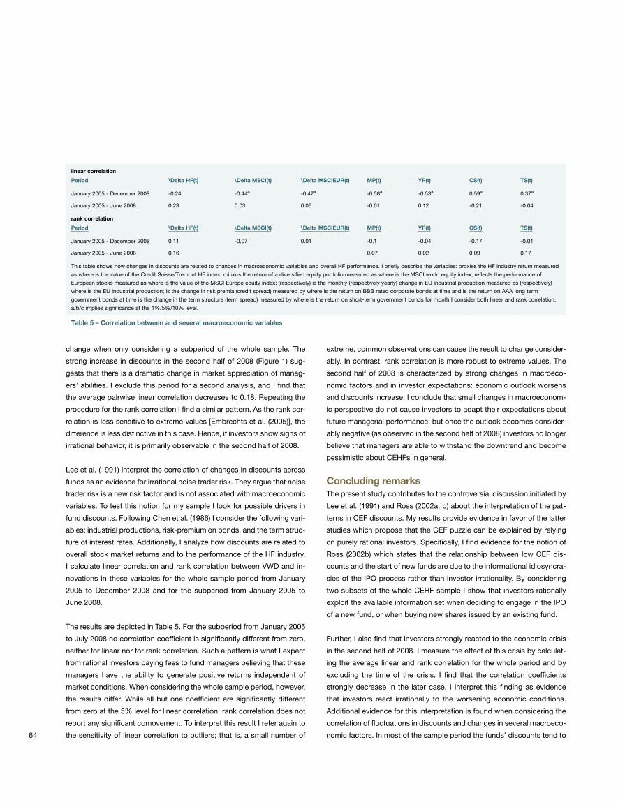
64

change when only considering a subperiod of the whole sample. The

strong increase in discounts in the second half of 2008 (Figure 1) sug-

gests that there is a dramatic change in market appreciation of manag-

ers’ abilities. I exclude this period for a second analysis, and I find that

the average pairwise linear correlation decreases to 0.18. Repeating the

procedure for the rank correlation I find a similar pattern. As the rank cor-

relation is less sensitive to extreme values [Embrechts et al. (2005)], the

difference is less distinctive in this case. Hence, if investors show signs of

irrational behavior, it is primarily observable in the second half of 2008.

Lee et al. (1991) interpret the correlation of changes in discounts across

funds as an evidence for irrational noise trader risk. They argue that noise

trader risk is a new risk factor and is not associated with macroeconomic

variables. To test this notion for my sample I look for possible drivers in

fund discounts. Following Chen et al. (1986) I consider the following vari-

ables: industrial productions, risk-premium on bonds, and the term struc-

ture of interest rates. Additionally, I analyze how discounts are related to

overall stock market returns and to the performance of the HF industry.

I calculate linear correlation and rank correlation between VWD and in-

novations in these variables for the whole sample period from January

2005 to December 2008 and for the subperiod from January 2005 to

June 2008.

The results are depicted in Table 5. For the subperiod from January 2005

to July 2008 no correlation coefficient is significantly different from zero,

neither for linear nor for rank correlation. Such a pattern is what I expect

from rational investors paying fees to fund managers believing that these

managers have the ability to generate positive returns independent of

market conditions. When considering the whole sample period, however,

the results differ. While all but one coefficient are significantly different

from zero at the 5% level for linear correlation, rank correlation does not

report any significant comovement. To interpret this result I refer again to

the sensitivity of linear correlation to outliers; that is, a small number of

extreme, common observations can cause the result to change consider-

ably. In contrast, rank correlation is more robust to extreme values. The

second half of 2008 is characterized by strong changes in macroeco-

nomic factors and in investor expectations: economic outlook worsens

and discounts increase. I conclude that small changes in macroeconom-

ic perspective do not cause investors to adapt their expectations about

future managerial performance, but once the outlook becomes consider-

ably negative (as observed in the second half of 2008) investors no longer

believe that managers are able to withstand the downtrend and become

pessimistic about CEHFs in general.

Concluding remarksThe present study contributes to the controversial discussion initiated by

Lee et al. (1991) and Ross (2002a, b) about the interpretation of the pat-

terns in CEF discounts. My results provide evidence in favor of the latter

studies which propose that the CEF puzzle can be explained by relying

on purely rational investors. Specifically, I find evidence for the notion of

Ross (2002b) which states that the relationship between low CEF dis-

counts and the start of new funds are due to the informational idiosyncra-

sies of the IPO process rather than investor irrationality. By considering

two subsets of the whole CEHF sample I show that investors rationally

exploit the available information set when deciding to engage in the IPO

of a new fund, or when buying new shares issued by an existing fund.

Further, I also find that investors strongly reacted to the economic crisis

in the second half of 2008. I measure the effect of this crisis by calculat-

ing the average linear and rank correlation for the whole period and by

excluding the time of the crisis. I find that the correlation coefficients

strongly decrease in the later case. I interpret this finding as evidence

that investors react irrationally to the worsening economic conditions.

Additional evidence for this interpretation is found when considering the

correlation of fluctuations in discounts and changes in several macroeco-

nomic factors. In most of the sample period the funds’ discounts tend to

linear correlation

Period \Delta HF(t) \Delta MSCI(t) \Delta MSCIEUR(t) MP(t) YP(t) CS(t) TS(t)

January 2005 - December 2008 -0.24 -0.44a -0.47a -0.58a -0.53a 0.59a 0.37a

January 2005 - June 2008 0.23 0.03 0.06 -0.01 0.12 -0.21 -0.04

rank correlation

Period \Delta HF(t) \Delta MSCI(t) \Delta MSCIEUR(t) MP(t) YP(t) CS(t) TS(t)

January 2005 - December 2008 0.11 -0.07 0.01 -0.1 -0.04 -0.17 -0.01

January 2005 - June 2008 0.16 0.07 0.02 0.09 0.17

This table shows how changes in discounts are related to changes in macroeconomic variables and overall HF performance. I briefly describe the variables: proxies the HF industry return measured

as where is the value of the Credit Suisse/Tremont HF index; mimics the return of a diversified equity portfolio measured as where is the MSCI world equity index; reflects the performance of

European stocks measured as where is the value of the MSCI Europe equity index; (respectively) is the monthly (respectively yearly) change in EU industrial production measured as (respectively)

where is the EU industrial production; is the change in risk premia (credit spread) measured by where is the return on BBB rated corporate bonds at time and is the return on AAA long term

government bonds at time is the change in the term structure (term spread) measured by where is the return on short-term government bonds for month I consider both linear and rank correlation.

a/b/c implies significance at the 1%/5%/10% level.

Table 5 – Correlation between and several macroeconomic variables

65

be unaffected by general economic influences. Such a pattern is what

I expect when trading in the CEFHs shares is mainly done by rational

investors. Note that HF managers justify their enormous fees by claim-

ing that they are able to generate positive returns independent of market

developments. Hence, a rational investor’s expectation about the fund

mangers’ ability must not be affected by macroeconomic factors. But

again, the investors strongly react to the worsening economic conditions

in the second half of 2008.

I conclude this chapter by emphasizing again that a similar discussion

is not possible with a sample of CEFs that exhibit a closely defined in-

vestment focus. The discounts of such funds are strongly affected by

the investors’ perception about the investment target of the funds, and

therefore a strong correlation for funds with a similar focus is not to be

interpreted as a sign for investor irrationality. Cherkes et al. (2005), for

example, find that IPOs of closed-end mutual funds in a specific sector

occur only during years in which seasoned funds in the respective sec-

tor are trading at a premium. A similar bias due to sectorial membership

does not appear in the present sample of CEHFs as HFs do not exhibit a

prespecified investment range.

References• Anderson, S. C., and J. A. Born, 2002, “Closed-end fund pricing, Dordrecht”, Kluwer

• Arora, N., N. Ju, and H. Ou-Yang, 2003, “An agency explanation of the closed-end fund

puzzles,” working paper, University of Maryland

• Berk, J. B., and R. Stanton, 2007, “Managerial ability, compensation, and the closed-end fund

discount,” Journal of Finance, 2, 529-556

• Bodurtha, J., D. Kim, and C. Lee, 1995, “Closed-end country funds and U.S. market

sentiment,” Review of Financial Studies, 8, 879-917

• Boudreaux, K. J.,1973, “Discounts and premiums on closed-end mutual funds: A study in

valuation,” Journal of Finance, 28, 515-522

• Brauer, G. A., 1993, “Investor sentiment and the closed-end fund puzzle: A 7 percent solution,”

Journal of Financial Services Research, 7, 199-216

• Chen, N., R. Kan, and M. H. Miller, 1993, “Are the discounts on closed-end funds a sentiment

index?” Journal of Finance, 48, 795-800

• Chen, N., R. Roll, and S. A. Ross, 1986, “Economic forces and the stock market,” Journal of

Business, 59, 383-403

• Cherkes, M., J. Sagi, and R. Stanton, 2005, “Liquidity and closed-end funds,” working paper,

U.C. Berkeley

• Chopra, N., C. M. Lee, A. Schleifer, and R. H. Thaler, 1993, “Yes, discounts on closed-end funds

are a sentiment index?” Journal of Finance, 48, 801-808

• Datar, V., 2001, “Impact of liquidity on premia/discounts in closed-end funds,” The Quarterly

Review of Economics and Finance, 41, 119-135

• DeLong, J. B., A. Shleifer, L. H. Summers, and R. J. Waldmann, 1990, “Noise trader risk in

financial markets,” Journal of Political Economy, 4, 703-738

• Doukas, J. A., and N. T. Milanos, 2004, “Investor sentiment and the closed-end fund puzzle:

out-of-sample evidence,” European Financial Management, 2, 235-266

• EBK, 2007, “Hedge-fonds, marktentwicklung, risiken und regulierung,” September, Swiss

Federal Banking Commission

• Elton, E., M. Gruber, and J. R. Busse, 1998, “Do investors care about sentiment?” Journal of

Business, 71, 477-500

• Embrechts, P., R. Frey, and A. McNeil, 2005, “Quantitative risk management: concepts,

techniques and tools,” Princeton University Press, Princeton

• Ferguson, R., and D. Leistikow, 2004, “Closed-end fund discounts and expected investment

performance,” Financial Review, 39, 179-202

• Lee, C., A. Shleifer, and R. H. Thaler, 1991, “Investor sentiment and the closed-end fund

puzzle,” Journal of Finance, 46, 75-109

• Lee, C., R. H. Thaler, and J. B. Shleifer, 1990, “Anomalies: closed-end mutual funds,” Journal of

Economic Perspectives, 4, 153-164

• Malkiel, B. G., 1977, “The valuation of closed-end investment-company shares,” Journal of

Finance, 32, 847-859

• Pontiff, J., 1996, “Costly arbitrage: evidence from closed-end funds,” The Quarterly Journal of

Economics, 111, 1135-1151

• Pontiff, J., 1997, “Excess volatility and closed-end funds,” American Economic Review, 87,

155-169

• Ross, S. A., 2002a, “Neoclassical finance, alternative finance and the closed-end fund puzzle,”

European Financial Management, 8, 129-137

• Ross, S. A., 2002b, “A neoclassical look at behavioral finance; closed end funds,” The Princeton

Lectures in Finance III

• Weiss, K., 1989, “The post-offering price performance of closed-end funds,” Financial

Management, 18, 57-67


67

PART 1

Next Generation Niche Markets

AbstractThis paper describes the development of an Internet-based

financing and web business development platform. It is the

first public internet supported straight-through-processing

(STP) model to be described for integrating the capital rais-

ing function with the development and operation of Internet

start-ups and maturing Internet businesses. The transpar-

ency demanded of secondary market traders/investors, usu-

ally afforded by audited periodic financial information and

research from independent analysts, has proven highly sus-

pect in past booms in Internet business start-up and devel-

opment activities. In the past cycle and to the present, web-

based, Internet-enabled businesses have been financed

through conventional money raising methods and, recently,

through Internet-based public auctions. The business itself

was detached from the money raising function and likewise

detached from secondary market trading. This paper will de-

scribe how to tightly couple the two, given that the financing

of the business and the business itself can be enabled on the

same information and communication technology platform.

Investors/traders can view price discovery of the company’s

shares at the same time and, where appropriate, on the

same screen as the web-enabled business. Statistics such

as number of visitors, purchases made, click-through pat-

terns, views, and other metrics of Internet businesses can sit

side by side with quotes and sales of the company’s shares.

The real-time nature of electronically auctioned primary mar-

ket fund raising, exclusively Internet-based businesses, and

secondary market trading allows for complete and absolute

transparency. This paper will, for the first time, describe how

investors/traders can see the books and records of a busi-

ness updated in real-time, observe the progress of the busi-

ness evolving in real-time, and observe the price of its shares

changing in real-time. A new information source, the “real-

time due diligence ticker” is also described.

Allan D. Grody – President, Financial InterGroup Holdings Ltd

Peter J. Hughes – Visiting Research Fellow, The York Management School, University of York

68

The business modelIn the past cycle and to the present, web-based, Internet-enabled busi-

nesses have been financed through conventional money raising methods

and, recently, through Internet-based public auctions. The business itself

was detached from the money raising function and likewise detached

from the secondary market trading. The challenge is to tightly couple

the two, given that the financing of the business and the business itself

can be enabled on the same information and communication technology

platform. Investors/traders can view price discovery of the company’s

shares at the same time and, where appropriate, on the same screen as

the web-enabled business.

Statistics such as number of visitors, purchases made, click-through pat-

terns, views, and other metrics of Internet businesses, collectively referred

to as due diligence data, can sit side by side with quotes and sales of the

company’s shares. The real-time nature of electronically auctioned primary

market fund raising, exclusively Internet-based businesses, and secondary

market trading allows for complete and absolute transparency, a desirable

attribute for potential investors and public company shareholders. Doing

so would enable investors/traders to see the books and records of a busi-

ness updated in real-time, observe the progress of the business evolving in

real-time, and observe the price of its shares changing in real-time.

We describe in this paper an integrated web-enabled business model that

incorporates: (1) an auction process for pricing a new or follow-on issue of

securities to fund either the start-up or continued operation of a web-based

business; (2) the secondary market trading of publically traded shares and/

or private placements of the web-based business; (3) a common set of

development tools for both managing the build-out and constructing the

web-based business; (4) a common platform to operate and monitor the

web-based business over the Internet; (5) a common platform for perform-

ing financing and banking activities, maintaining the books and records,

and auditing the web-based business; and (6) a management information

system that oversees each of the web-based businesses for security, reli-

ability, capacity and usage, and fraud monitoring and detection.

The business model is extended to support primary and secondary mar-

ket functions by incorporating: (1) a common business plan and presenta-

tion framework and proposal development tool kit for preparing “offering

memorandum” and road shows; (2) a common book running/syndication

framework and system; (3) a market making, trading and/or automated

price matching system for price dissemination and secondary market

trading; and (4) a common communication platform where traders/inves-

tors can communicate with others (shareholders, potential shareholders,

peers, etc.) using real-time, voice-over-Internet protocols (VOIP) and in-

stant messaging technologies (chat rooms, blogs, broadcasts, etc.). Such

communication can allow ratings/reviews of either the company or the

stock itself, i.e., product/service, value of share price, etc., with all such

communications being logged and accessible, thereby deterring market

manipulation.

For the first time, a going business will produce and distribute real-time

due diligence data, bringing assurances to the investor/trader that the web

business owner receiving funds is tightly coupled in an STP processing

model to an external, independent continuous audit function and, further,

to an accounting firm to actually oversee and/or post journal entries for

cash and valued collateral to each web businesses’ official books and re-

cords. A bank or banks with global reach is tied into the system electroni-

cally in the same STP model and a local audit/account partner must be

a dual signer to allow the web business owners access to funds so that

financial fraud is mitigated.

Finally, the software platform, communications infrastructure, power grid,

and any call center facility, etc. must be accommodating of a 24/7, high

availability, secure facility that supports both function-rich websites and

the mechanisms to accept payments for product and service purchases,

and/or marketing activity for advertisers, as well as supports a secure, well-

regulated primary and secondary market issuance and trading structure.

BackgroundInternet pioneers E*Trade and Wit Capital, along with traditional investment

bankers turned e-commerce entrepreneurs, created a more even playing

field for the individual investor in garnering a fairer share of IPOs back

in the late 1990s at the dawn of the Internet age when a research and

defense network established by the U.S. Government was turned over to

commercial interests. Wit Capital began offering IPOs to their Internet cli-

ents by placing an offering document on the newly developing Internet in

1995. Its intention at that time was to solicit interest in the sale of shares in

its own company, Spring Street Brewing. At that time, Wit was the brand

name of the beer brewed by Spring Street Brewing Company. Being the

first to present a public offering document over the Internet, the company

■■ Real-time production and distribution of data for public company due

diligence.

■■ Contiguous and simultaneous production of above with real-time market

data.

■■ Contiguous and simultaneous availability of real-time due diligence data

for real-time IPO price discovery and transparency of public company

securities.


for real-time secondary market price discovery and transparency of public

company securities.


of public companies for real-time IPO pricing, and real-time secondary

market price discovery and transparency.

Figure 1 – The integrated business and capital raising model

69

soon attracted media attention and a host of investors. This early success

spurred the founder of the brewery to quickly realize the benefit of under-

writing other companies’ issues for promotion over the Internet. Wit Capital

eventually participated with traditional underwriters and received a portion

of the allocation for distribution to its clients, which had mainly been at-

tracted to Wit through its early Internet presence.

Another group, E*Offering, a venture of E*Trade, and investment bankers

Sanford Robinson and Walter Cruttenden, attempted to distribute 50%

of an IPO to the individual investors that came through E*Trade’s online

brokerage service. They expected that online road shows and prospec-

tuses would lower the distribution cost eventually from the then current

standard of 7% to 4%. Fast forward to today where, in the U.S., fees to

take a company public have stayed at an average 6.7% of the proceeds

of the offer. This compares with banks in Europe, which bill their clients

an average of 3.2%, and Asia, where underwriters typically pocket about

2.5% of the proceeds.

Their approach did not attempt to solve the problem of the mispricing of

new issues where the price of the stock on the first and subsequent days

of secondary market trading reached unprecedented heights. This simply

allowed E*Trade clients, like Wit Capital clients, to become part of the

privileged few that enjoyed the benefits of the large run-ups in the early

days of secondary market trading in those mispriced issues.

Another venture, that of William Hambrecht’s W. R. Hambrecht & Co., set

IPO prices and allocation of IPOs online through an auctioning process

known as a Dutch auction. This facility, known as OPENIPO, allowed

bidders to open brokerage accounts with W.R. Hambrecht & Co. or the

other brokerage firms participating. Bids were taken for the number of

shares wanted and at the price the bidder was willing to pay. After a few

weeks of accepting bids, the offering price was set at the lowest price at

which all shares could be sold, known as the clearing price. Those who

bid above the offering price would get all the shares they asked for at the

offering price, while those bidding at the offering price would get some

portion of their shares, and those bidding below would not receive any

shares. No single bidder could receive more than 10% of the offering and

the underwriter would reserve the right to limit the maximum amount to

as little as 1% per shareholder. This last approach represents a real solu-

tion for IPO mispricing by making it possible to allow all available demand

into a primary market “auction” and, thus, be able to set the most bal-

anced initial public offering price.

The most memorable IPO auctioned in this way was that of Google, itself

a web-based business model, in 2004. Notwithstanding the improved

access afforded to bidders, the offering still fell short of accommodating

all the demand in the market, as witnessed by the subsequent day’s sec-

ondary market trading which saw a further run up in Google’s stock price.

The logic behind such an approach is that it would allow all investors

to bid for Google’s shares directly, rather than leave it to an investment

bank to decide on the price of the shares and who should receive them –

usually their biggest institutional clients. It also reduces the amount of

underwriting fees, which, in theory, should ensure the company gets a

larger share of the proceeds of an IPO. Critics, however, warned that an

auction could risk setting an unrealistically high price for Google’s shares

since there would not be enough stock available to meet the massive

demand from private investors captivated by the prospect of a new dot-

com gold rush.

Google’s IPO technique flopped and it underpriced the shares. Bankers

drummed home the message that money saved in underwriting fees was

dwarfed by the amount Google left on the table through the underpricing.

It is a painful argument to swallow, especially given the behavior of banks

during the dot-com boom of 1998-2000. Back then, critics accused them

of underpricing IPOs – discounting the share price on the day of the of-

fering – to curry favor with the institutional buyers, effectively failing to

maximize profits and leaving money on the table. An estimate of an ag-

gregate of U.S.$62 billion was left on the table in U.S. IPOs carried out

between 1999 and 2000.

At its peak, about 250 companies went public in 2000 in the U.S., a num-

ber that plummeted when the dot-com bubble burst, before crawling back

to 75 IPOs in 2007. The economic downturn made it even worse, with

no U.S. venture capital-backed company going public for six months until

April 2009, when Bridgepoint Education Inc. made its debut. The online

auction process was similar in concept to what the Tokyo Stock Exchange

(TSE) had been doing since 1993, which was abandoned after the Internet

bubble affectively ended the plethora of new issuances. The TSE used an

auctioning procedure for approximately 50% of the offered shares. Under

their procedures, an investor who bid highest would receive their shares at

their bid price; the next highest bidder would receive their shares at their

bid price, etc. This “price discriminatory” auction continued in this way

until all shares allocated to the bidding process were priced. Thereafter,

the weighted average bid price was used to set the offering price of the

remaining shares unallocated to the auction process.

By limiting the offering bids to 5,000 shares per order, both in the auction

and in the subsequent allocation, the IPO was widely distributed. Also,

results have shown that in the initial early days of trading returns fell from

an average of a 70% rise prior to the installation of this new auction pro-

cedure to approximately 12%. The TSE had modified their procedures to

allow both traditional underwritings as well as auctions, with the issuer

able to choose between the two. At the end of the experiment, half of

the TSE’s IPOs were auctioned and half were done through traditional

underwritings.

The Capco Institute Journal of Financial TransformationNext Generation Niche Markets

70

Angelsoft (www.angelsoft.net) Angelsoft provides web-based deal-flow and portfolio management tools for finding, accepting, tracking, and collaborat-ing on early stage investments for use between en-trepreneurs, angel investors, and venture capitalists. Angelsoft lets investors accept new deal opportuni-ties and track them over the web, by email or through a customizable application process integrated into a client’s own website. It provides a secure platform and reporting mechanism to collaborate among in-vestors and includes message boards, document management, event management, and deal access control for every deal “room.” Entrepreneurs can post business plans in online deal rooms, develop pitches and secure online deal processing systems through which investors collaborate to review business op-portunities using the latest due diligence technolo-gies. It then connects them, ties them directly into the world’s leading organizations of professional invest-ment funds, and supports them with the participation of top tier venture law firms, business schools, and investment conferences.

By providing one platform that connects everyone in the early stage investment world, they bring transpar-ency to early stage investing. Entrepreneurs can view real-time statistics on potential investors. Investors can find experts in specific industries and give a pitch a thumbs-up or thumbs-down. Additional premium features include searchable databases, promotional opportunities, and investment support services. It claims to have over 19,000 early stage investors managing their investments through over 450 venture funds and angel groups from 45 countries collaborat-ing on thousands of new funding applications each month.

InTrade (http://www.intrade.com/) – InTrade (U.S.A.) is a division of the Minneapolis Grain Exchange, which confers on InTrade regulated exchange sta-tus under the CFTC. Their trading service allows members to transact trades on political, financial, current, and similar event futures. InTrade provides the platform whereby members can trade between themselves. InTrade ensures that trading profits and losses are transferred between customers in a timely manner and allows customers to close out positions by trading with any other customer. InTrade has been developed around a combined exchange and clear-ing house model. There is no charge for entering an order; there is only a commission when a matched trade occurs.

The market data that is produced from this trading is used by people who want to acquire the predic-tive intelligence from the InTrade marketplace. They include governments, global media organizations, central banks, investment houses, universities, the military, private traders, consultancies, and public in-dividuals. For example InTrade supplies market data to CNBC, CNN, FOX, WSJ, FT, New York Times, a number of Federal Reserve Districts, major universi-ties and graduate schools in the U.S., the ECB, Cato, Bank of Japan, Bank of England, presidential candi-dates, and major and boutique Wall Street firms. They operate public and private prediction market places for Yahoo!, The Financial Times, the National Journal,

RealClearPolitics, and Rasmussen Reports. These marketplaces increase page views, editorial content, community, user “stickiness,” average time on a site and therefore increase advertising revenue.

Prosper (http://www.prosper.com/legal/compliance.aspx) – The Prosper marketplace is a peer-to-peer online credit auction platform operated by Prosper Marketplace Inc. (“Prosper”), a registered financial company. Prosper handles the registration of bor-rowers, lenders, loan sellers, and group leaders; the receipt, display, and matching of listings and bids on listings; the issuance and sale of Borrower Payment Dependent Notes to lender members; and the origi-nation, servicing, and collection of principal, interest, and other charges payable on loans. Lender members may offer their Notes for sale to other lender members through the Folio Investing Note Trader platform oper-ated and maintained by FOLIOfn Investments Inc., a registered broker-dealer.

Borrower members can post listings on the platform to request and obtain loans. Lender members can bid on listings and purchase Notes from Prospers that are dependent for payment on payments received on the corresponding borrower loans described in the listing. Group leader members can form groups of borrowers with common interests.

All loans originated through the platform are made by WebBank, a Utah chartered Industrial Bank and sold and assigned to Prosper. Prosper provides services to WebBank in connection with the origination of these loans. Prosper services all loans made to borrowers on behalf of lender members who purchase Notes. The payments of the Notes are dependent on the cash flow from the loans. All borrower loans are fixed-rate, unsecured, 3-year, fully amortizing with simple interest. All loans are obligations of individual borrow-ers and not of corporations or businesses. A borrower who obtains a loan to be used for business purposes is personally obligated to repay the loan, regardless of the success or failure of the business for which the loan may be used.

SecondMarket (http://www.secondmarket.com/) – SecondMarket bills itself as the largest centralized marketplace and auction platform for illiquid assets, such as auction-rate securities, bankruptcy claims, collateralized debt obligations, limited partnership interests, private company stock, residential and commercial mortgage-backed securities, restricted securities, and block trades in public companies and whole loans. SecondMarket’s online auction platform claims over 5,000 participants, including global finan-cial institutions, hedge funds, private equity firms, mutual funds, corporations, and other institutional and accredited investors that collectively manage over U.S.$1 trillion in assets available for investment. Their hybrid transaction model uses technology and sales and trading professionals to offer liquidity in il-liquid markets. Their online trading platform provides a centralized location to bring buyers and sellers to-gether and provide transparency and offer a variety of auction formats including English auctions, Dutch auctions, sealed bid auctions, reverse auctions, and SecondMarket’s patent pending ManhattanAuctions.

Further, their trading platform utilizes a proprietary matching algorithm to pair buyers and sellers. Sec-ondMarket facilitates all administrative and settlement support services for executing both private and pub-lic transactions involving illiquid assets. They man-age the entire process, from pre-sale due diligence through execution and settlement.

Kiva (http://www.kiva.org/about/how/) – Lenders browse profiles of entrepreneurs in need and choose someone to lend to. When they lend, using PayPal or their credit cards, Kiva collects the funds and then passes them along to one of their microfinance part-ners worldwide. Kiva’s microfinance partners distrib-ute the loan funds to the selected entrepreneur. Their partners also provide training and other assistance to maximize the entrepreneur’s chances of success.

The Receivables Exchange (www.ReceivablesX-change.com) – The Receivables Exchange claims to be the world’s first online market place for real-time trading of commercial accounts receivable. It provides small business financing for working capital manage-ment. The Exchange connects a global network of ac-credited investors (buyers) to the U.S.’s three million small and mid-sized businesses (sellers) in search of capital to grow their businesses. Buyers get direct ac-cess to an U.S.$18 trillion new investable asset; small businesses get to access a new competitive working capital management solution by having their receiv-ables bid on by multiple buyers in real-time.

UnifiedMarkets (UM) (http://www.unifiedmarkets.com/) – UM offers global access to financial and busi-ness information and access to worldwide listings of service providers, including securities settlement and trust service operators. Indications of Interest (IOI) to buy and sell an unprecedented range of assets are posted by members on UM including all types and classes of securities, businesses, business assets, business loans, and joint ventures. UM member ser-vices include links to independent, broker-operated on-line trading systems that accept firm buy and sell quotes and provide securities auction services. UM is an Internet-based, 24/7 worldwide network. The search engine locates UM member IOI postings of financial instruments, businesses, business assets, and other assets that are of interest. UM members post IOI for purchase and sale of unregistered and registered financial instruments, businesses, and business assets. Members may limit the scope of IOI distribution and search access to only other members who meet certain qualifications specified by them. Members may further target or restrict their IOI distri-bution and search to pre-designated affinity groups. The online confidential and encrypted discussion groups that are supported for anonymous meetings, discussions, and negotiations are deleted from the UM databases following conclusion of discussions. There is no investment advice provided by UM to members, UM members do not effect transactions on UM and members are advised to use licensed agents of their choice for transaction settlements.

Figure 2 – Niche market examples

71

The Tel Aviv Stock Exchange, after installing a new electronic trading

system, had also adopted an auction procedure for IPOs, known as a

Uniform Price Auction, similar to the Dutch auction of W.H. Hambrecht.

These auctions resemble the auctions conducted by the U.S. Treasury,

where U.S. Treasury securities are issued.

Today, the Internet provides access to a wider distribution base, making

broad primary electronic offerings possible. An electronic primary auction

process in an integrated system with a secondary market trading method

and a transparent Internet operating, marketing, and financial business

model (collectively, the STP process described in this business model) is

a logical extension of systems and communications capabilities coupled

with a web community of informed investors.

Other business modelsOther models for Internet-based capital raising, trading, and fulfillment

exist, some of which are described below. While there are many varia-

tions of this proposed business model, some going back to the begin-

nings of electronic market trading systems, from the early days of Instinet

and CATS to the automated contract markets of Intex and Globex, none

integrated an initial offering (IPO) process to finance any start-up or sec-

ondary offering. None anticipated a niche market with web-based busi-

nesses. Also, there was no attempt to create real-time due diligence data

to observe the ongoing operations, marketing or financial activities of a

business now made possible by web-based businesses.

None of the existing or proposed business models have integrated the

business of the underlying financed company into the exchange systems

platform, nor an ability to view both IPO financing and secondary market

trading at the same time as viewing real-time due diligence within a web-

based business model on the same platform.

Description of the web-enabled market and business model (WMBM)A business entrepreneur will either present an idea, a business plan, a

prototype of a web-based business, or a partial or fully functioning web-

based business. The initial process of the WMBM described below re-

quires an evaluation of the business model and, if judged acceptable

based upon the WMBM’s own business criteria, will prepare the nec-

essary materials (presentations, pitch book, business plans, etc.) for its

financing through its advanced web-based business tools. Based upon

the web-based platform(s), tools, and vendor applications imbedded in

the prototype or the partial or fully functioning web-based business, a

plan to transfer, convert, and/or build features and functions into or for

the business will be undertaken.

As with all new issues, an issuing company would proceed to prepare an

offering document with all the traditional financial measures, valuation

procedures, and public filings. The shares would be posted for offering on

an electronic “book” that supports the issuance method of the WMBM.

In this instance, the book would simply be used to store and price new

issues rather than already issued securities – conceptually a new ap-

plication of the existing mechanism for the opening of the day’s trading

for already issued securities on existing exchanges. Prior to placing an

anonymous bid, the bidder would access company and due diligence

information via the Internet, placed there by the sponsoring broker under

the WMBM and by the issuing company through its designated website.

Traditional brokerage firms, along with Internet-based and other online bro-

kerages, would provide electronic interfaces between the customer orders

coming into it and the orders being placed on the system of the WMBM for

the initial offering of the company’s shares. Following the acceptance of an

order, an account would be opened pending the receipt of funds. For exist-

ing account holders, sufficient funds would be checked prior to accepting

an order and segregated for placement on the exchange.

The auction process would be programmed to proceed in any of a num-

ber of ways described earlier in a number of auction processes: Dutch

auction, English auction, sealed bid, reverse auction, Vickery auction,

etc. The offering can be updated to reflect the demand by either making

more shares available (as is common with “shelf registrations” in the U.S.)

and/or keeping the shares at the initial number while accepting only the

highest priced bids until all demand is satisfied. The amount thus raised

would be transferred to the company issuing the shares and the official

start of secondary trading would commence.

The opening trade price would be determined through first accepting

and then matching bid and offer prices and size until an equilibrium price

is determined from which all at-opening orders would be filled. These

prices would be disseminated through the WMBM and through commer-

cial market data vendors, which would then proceed in a more orderly

Acceptance of web business model and initiation of IPO process

Preparation of business plan, pitch book,

online road show material

Initial auction pricing and financing module

➞

Development of and/or operation of web business

Financial, operating and marketing metrics

modules

Secondary market trading module

➞

External Interfaces, monitoring, security, and compliance

Banking, auditing and accounting modules;

compliance, regulatory reporting and

monitoring; security and availability;

network management

Order and market data management,

due diligence distribution, road show

distribution, discussion groups, research

and news services; call center management

Figure 3 – Overview of web-enabled market and business model

The Capco Institute Journal of Financial TransformationNext Generation Niche Markets

72

fashion, moving up or down as bids at a certain price seek offers at or

near the same price, somewhat tied to the perceived fortunes of the

company. The fortunes of the company would be observable through the

transparent nature of the operations, financial activities, and marketing

metrics available on the system.

The web-based business will be integrated into the above financing func-

tion and secondary market trading functions such that the businesses’

operating, marketing, and financial metrics will be transparent and ob-

servable on the integrated platform

Measures for assuring that no information leakage occurs, such as insid-

er trading; or financial leakage, such as theft of financial assets; or fraud

occurs will be integrated into the platform and closely monitored. For

example, the web business owner receiving funds must use the WMBM’s

method of approved local audit/account partner as a dual signatory. All

fund movements are tightly coupled by a systematized, external, inde-

pendent, and continuous audit function and an accounting firm to actu-

ally oversee and/or post journal entries for cash and valued collateral to

each web businesses’ official books and records for those that do not

come from electronic payment and/or inventory management systems.

A bank(s) with global reach is tied into the system electronically so that

financial fraud is mitigated.

ConclusionThe web-enabled market and business model suggested in this paper

will help entrepreneurs, as well as established corporations, to find a new

shareholder class on the Internet. Not only a class of shareholder that

comes to appreciate a new web-based business, but also those who

shop or use services of the internet businesses of established corpora-

tions. In an earlier era of Internet start-ups such companies were spun

off, in an accounting sense, from the parent and offered to a new invest-

ing group as a new share offering called a tracking stock. The model

described in this paper will assist both start-ups and fully formed compa-

nies in the coming era of web-enabled businesses to reach a new share-

holder class, the internet consumer of digital services.

Peter Lynch, the legendary portfolio manager of Fidelity’s Magellan fund,

was fond of advising individuals to buy stocks of companies that they

frequent as a consumer. Our advice is similar: buy the stocks of those

web-enabled businesses that you frequent, and also buy these stocks

where you shop – on the Internet!

Figure 4 – Dashboard display for observing the integration of real-time due diligence with real time price discovery and transparency

73

PART 1

Global Financial Centers – Growth and Competition after the Crisis

AbstractInternational competition between financial centers is fierce,

and the financial crisis is set to accelerate the pace of change.

U.S. and E.U. financial markets continue to provide around

three-quarters of global financial services, albeit, after the

crisis, at substantially lower overall levels of market activ-

ity in many market segments. Emerging financial markets,

especially in Asia, have grown strongly in past years and are

expected to continue on this path going forward. Emerging

financial centers such as Beijing, Seoul, Shenzhen, Shanghai,

and Dubai have improved their global rankings strongly since

2007, raising their competitiveness ratings by 42% for Seoul,

27% for Beijing, 22% for Mumbai, and 16% for Shanghai.

Going forward, four drivers of financial center competitive-

ness after the crisis can be identified: 1. Big is beautiful – and

will remain so. London, New York, Hong Kong, and Singa-

pore are set to remain strongholds of global finance after

the crisis, building on existing market strength and favorable

economic conditions. 2. There is a trend towards a multi-

polar financial industry. In the long run, emerging financial

centers are likely to succeed in establishing the scale and

scope in their market environments that will help them ad-

vance into the top group of global locations. The crisis may

accelerate this trend. 3. National focus will serve as transi-

tory advantage for smaller centers. Local and regional finan-

cial marketplaces may hope for continued relevance owing

to the refocusing of market participants and policymakers

on their national markets. However, this tailwind will likely be

of limited duration. 4. Good regulation will be a competitive

advantage. Providing a good regulatory framework will be a

key determinant of competitiveness going forward. Financial

centers not compliant with international rules are faced with

increasing political pressure and stigmatization.

Steffen Kern – Director, International Financial Markets Policy, Deutsche Bank AG

74

Financial centers are not easily shaken. They develop over long cycles.

Even when financial markets turn nervous or economic conditions sour,

the pivotal role of financial centers for their business environment mostly

remains intact. Key financial centers around the world have grown sub-

stantially over the past decades, supporting and benefitting from the de-

velopment of the surrounding economies at the same time. The share in

value added in the home economies has increased significantly in most

advanced and emerging markets.

After an event of the magnitude and intensity of the recent financial crisis,

however, it is worthwhile examining its potential impact on the structures

and business prospects of the major financial centers around the world,

and assessing their likely course of development in future. Clearly, the

performance of financial centers represents a vital part of the business

conditions in which companies across all industries operate, and it there-

fore carries wider implications for other sectors, employment, and the

economy. Although the final impact of the crisis on financial centers will

only be observable at a later stage, this article reviews the current state of

development of key advanced and emerging financial centers and identi-

fies drivers of competitiveness for the coming years.

Global landscape of financial centers after the crisisThe financial crisis, despite its impact especially in the U.S. and Europe,

has not immediately led to a critical change in the tectonics among the

major financial centers around the globe so far. The traditional financial

centers in the U.S. and the E.U. have managed to retain their strong dom-

inance and continue to provide around three-quarters of global financial

services, even if at substantially lower overall levels of market activity in

many market segments.

Banking – well over two-thirds of global banking assets remain concen-

trated in financial centers in the U.S. and the E.U. [Transatlantic Business

Dialogue (2010)]. Together, they capture more than three-quarters of the

global revenue pool of investment banking services [International Finan-

cial Services (2010)].

Stock markets – at almost two-thirds of global stock market capitaliza-

tion, the share of the traditional stock exchanges in the U.S., the E.U.,

Japan, Hong Kong, and Singapore remains dominant, albeit consider-

ably lower than their 90% peak in 2000.1 Their 79% share in global equity

trading, however, documents their strong position as the key equity trad-

ing centers worldwide.2 Moreover, U.S. and E.U. equity-linked derivatives

make up more than three-quarters of the global outstanding [Transatlan-

tic Business Dialogue (2010)].

Debt instruments – more than 70% of all private and public debt se-

curities and almost 80% of all interest-rate derivatives outstanding are

registered in the traditional financial centers in the U.S. and the E.U.

[Transatlantic Business Dialogue (2010)]. Almost three-quarters of all new

international debt securities are issued in New York or the major financial

centers in Europe.3

Foreign exchange – foreign exchange trading remains highly concen-

trated in London and Chicago, with the U.K. and the U.S. capturing a

combined 50% share in global trading. 70% of all foreign exchange de-

rivatives transactions are undertaken in the U.S and the E.U. [Transatlan-

tic Business Dialogue (2010)].

These impressive figures, however, cannot belie the fact that the historic

position of the traditional financial centers in Europe and America is in-

creasingly being challenged by emerging competitors.4 Equity markets

are an illustrative and in large parts representative example: the transat-

lantic share in global stock market capitalization has declined substan-

tially from its 78% peak in 2001 to just over 50% today, while their share

in stock trading has fallen from 86% to just over 70% in the same period.5

1 World Federation of Exchanges and own calculations.

2 Ibid.

3 Bank for International Settlements and own calculations.

4 For a detailed analysis of the role of U.S. and EU financial markets in the world economy

see Kern (2008), also TABD (2010).

5 World Federation of Exchanges and own calculations.

0

50

100

150

200

250

300

350

90 95 00 05 10E

Securitized assets

Commercial real estate

Bank assets

Debt securities

Stock market capitalization

y = 2.6313e0.0459x

R² = 0.5114

0

5

10

15

20

25

30

35

40

45

0 15 30 45

% change in rating 2007-2010

Ranking 2007

42

27

23

22

16

11

9

8

8

5

3

3

2

2

2

1

0 20 40 60

Seoul

Beijing

Moscow

Mumbai

Shanghai

Singapore

Tokyo

Dubai

Hong Kong

Amsterdam

Zurich

Paris

Frankfurt

New York

Cayman Islands

London

0

10

20

30

40

50

60

00 02 04 06 08

US

EU

JP

BRIC

Other Asia

41

10 6

- 3 - 4 - 5

-20

0

20

40

60

BR

IC

Oth

er

Asi

a

Oth

ers

EU JP US

Note: Share of market capitalization of domestic listed companies, % of global total, and

CAGR 00-10

Sources: World Federation of Exchanges, DB Research

Figure 1 – Decline of traditional stock markets

75

Neither the ranking nor the competitiveness rating of these centers has

changed significantly over the past years. Marginal changes aside, the

composition of top league tables has been comparatively static, while im-

provements in their ratings – at between 1% and 3% for London, New

York, Frankfurt, and Paris between 2007 and 2010 – have been marginal.

What may be described as continuity in the performance of these finan-

cial centers contrasts sharply with the rise of emerging financial markets.

Emerging financial centers such as Beijing, Seoul, Shenzhen, Shanghai,

and Dubai have improved their global ranking strongly since early 2007,

jumping 20, 17, 14, 13, and 4 places up the global league table10, re-

spectively. Even more impressively, the competitiveness rating of these

financial centers has progressed dramatically, rising by 42% for Seoul,

27% for Beijing, 22% for Mumbai, and 16% for Shanghai.

These and other emerging financial centers have succeeded in exploit-

ing the catch-up process to the traditional trading centers. Accordingly,

the improvement in competitiveness ratings between 2007 and 2010 are

closely correlated with the initial ranking of the centers.11

Financial centers have been categorized to capture their development.

Most analyses differentiate the geographic reach of individual centers as

well as level of maturity that they have reached. At one extreme, mature

financial centers with a global dimension are found to include Chicago,

Frankfurt, Hong Kong, London, New York, Singapore, Toronto, and Zu-

rich. At the other end of the scale cities such as Budapest, Istanbul, or

Riyadh are considered to be local in scope and at an early stage of their

development as broad and deep financial markets. In between, a broad

variety of combinations of geographic reach – from local to transnational

and global – and degree of development – from emerging to mature –

have been identified. Much of the dynamism in competitiveness rank-

ings and ratings discussed here can so far be observed in the lower and

middle ranges of the league tables.

Strikingly, the growth of stock markets in the BRIC countries amount to

more than 40% per year, while the E.U. and U.S. markets actually con-

tracted.6 Likewise, the share of the BRIC countries in the number of listed

companies worldwide has jumped from just over 2% in 2000 to 22%

today.7 More than half of the world’s IPOs in 2009 were listed in China

alone8 [Kern (2009)]. Similarly, Asia’s share in the investment banking rev-

enue pool has risen from 13% in 2000 to more than 20% in 2009 [Inter-

national Financial Services (2010)].

In light of these long-term trends, it is evident that traditional financial

centers, including New York, London, Paris, Zurich, but also Hong Kong

and Singapore are facing heightening pressure to maintain their roles.

Financial center competitionThe competitive position of the major financial centers around the world

mirrors these trends. Traditional financial centers have grown to strength

over decades and are repeatedly found to rank top in terms of interna-

tional competitiveness. A typical top-10 ranking of financial center com-

petitiveness includes London, New York, Hong Kong, Singapore, Tokyo,

Chicago, Zurich, and Geneva among the front-runners.9 Other financial

centers in the advanced economies such as Sydney, Toronto, Frankfurt,

Boston, San Francisco, Washington, Luxembourg, Paris, or Vancouver

consistently rank among the top-25.

1 to 20 21 to 40

London Melbourne

New York Montreal

Hong Kong Cayman

Singapore Edinburgh

Tokyo Seoul

Chicago Dublin

Zurich Hamilton

Geneva Amsterdam

Sydney Stockholm

Shanghai Brussels

Toronto Copenhagen

Frankfurt Vienna

Boston Wellington

Beijing Madrid

San Francisco Oslo

Washington Milan

Luxembourg Rome

Paris Helsinki

Vancouver Mumbai

Dubai Prague

Note: Top-40 ranking of financial centers according to GFCI.

Sources: City of London, DB Research

Figure 2 – Ranking of top financial centers worldwide

6 Ibid.

7 Ibid.

8 Figure includes Hong Kong SAR. International Financial Services (2010), p. 8.

9 City of London (2010), p. 28. The ranking reproduced here is the City of London’s Global

Financial Centers Index (GFCI), published bi-annually since 2007, and ranking 75 financial

centers around the globe on the basis of indicators for availability of human resources,

business environment, market access, infrastructure, general competitiveness, and assess-

ments by market participants. The relevant data in this article are taken from Global

Financial Centers 7 of March 2010. The September 2010 edition of the GFCI confirms the

conclusions of this article. Alternative approaches include, the World Economic Forum’s

Global Competitiveness Report, in which measures for financial market development,

financing through local equity markets, ease of access to loans, venture capital availability,

restrictions on capital flows, strength of investor protection, soundness of banks, regulation

of securities exchanges, and legal rights are summarized to obtain an index for financial

market sophistication for 133 countries. Financial centers are not analyzed individually. See

World Economic Forum (2010), p. 337 ff.

10 City of London (2010), p. 28. Changes in ranking adjusted for new entries and drop-outs.

11 The close correlation exists for the percentage change in GFCI rating points between 2007

and 2010 and the ranking of financial centers in 2007 (r=0.71).

The Capco Institute Journal of Financial TransformationGlobal Financial Centers – Growth and Competition after the Crisis

76

However, it is worthwhile noting three important caveats. First, as much

as they still dominate, the top ranks in competitiveness league tables

are no longer the prerogative of traditional financial centers. Most impor-

tantly, Shanghai, Beijing, and Dubai have successfully advanced to the

top group of competitive financial centers even if in terms of market size

and maturity they still belong to the emerging centers.

Second, European financial market places are on the whole falling be-

hind in the rankings. Thus, cities such as London, Paris, Madrid, Milan,

Frankfurt, and Amsterdam have clearly lost grounds compared to other

advanced and emerging locations, and, in particular, seem to be missing

opportunities of enhancing their competitiveness.

Finally, empirical assessments of financial sector competitiveness have

yielded varying and at times contradicting results.12 Depending on the

criteria applied when measuring competitiveness, market maturity, so-

phistication, or other indicators, financial centers can exhibit very differ-

ent stages of development.

Despite the significant variations in classifying financial centers, there is

broad agreement on the factors that explain the emergence and devel-

opment of financial markets, and that can help promote the competitive-

ness of individual financial centers. At a more general level, financial mar-

kets develop along real economic needs, with the financing of trade and

commerce, the mobilization of capital in light of economic competition,

or the protection of assets in unstable economic environments as basic

fundamental motivations [Arner (2008)]. On the basis of these needs, fi-

nancial center development benefits if a number of conditions are met

which facilitate the emergence of a network-type market place. These

basic conditions13 include:

■■ Innovative and competitive financial intermediaries.

■■ Solid market infrastructure for communication and financial transac-

tions.

■■ Widely available information.

■■ Free capital flows and open access to domestic and international

markets

■■ Access to related professional services.

■■ Qualified human resources.

■■ Sound monetary and exchange rate framework.

■■ Stable political institutions.

■■ Rule of law and calculable business environment.

■■ Efficient regulatory and supervisory arrangements.

■■ Friendly tax environment.

■■ Quality of life.

In combination, economic and business needs as well as these condi-

tions for financial developments greatly influence the success of financial

centers, with a wide range of possible outcomes for individual market

places. In practice, the key question is, how these factors combine and

12 The indicator for financial market sophistication in the World Economic Forum’s Global

Competitiveness Report, for example, produces a very different ranking of financial markets

and their centers, among other things ranking the U.S., the U.K., and a number of European

financial markets below countries such as India and Montenegro in terms of sophistication

[World Economic Forum (2009)].

13 Arner (2008), pp. 196-200. The importance of individual conditions varies along the state of

development of individual financial markets and centers.

0

50

100

150

200

250

300

350

90 95 00 05 10E

Securitized assets


Bank assets

Debt securities


y = 2.6313e0.0459x

R² = 0.5114

0

5

10

15

20

25

30

35

40

45

0 15 30 45


Ranking 2007

42

27

23

22

16

11

9

8

8

5

3

3

2

2

2

1

0 20 40 60

Seoul

Beijing

Moscow

Mumbai

Shanghai

Singapore

Tokyo

Dubai

Hong Kong

Amsterdam

Zurich

Paris

Frankfurt

New York

Cayman Islands

London

0

10

20

30

40

50

60

00 02 04 06 08

US

EU

JP

BRIC

Other Asia

41

10 6

- 3 - 4 - 5

-20

0

20

40

60

BR

IC

Oth

er

Asi

a

Oth

ers

EU JP US

Note: Change in competitiveness index between 2007 and 2010, % change of GFCI ranking

for selected centers


Figure 3 – Emerging financial centers enhance competitiveness

0

50

100

150

200

250

300

350

90 95 00 05 10E

Securitized assets


Bank assets

Debt securities


y = 2.6313e0.0459x

R² = 0.5114

0

5

10

15

20

25

30

35

40

45

0 15 30 45


Ranking 2007

42

27

23

22

16

11

9

8

8

5

3

3

2

2

2

1

0 20 40 60

Seoul

Beijing

Moscow

Mumbai

Shanghai

Singapore

Tokyo

Dubai

Hong Kong

Amsterdam

Zurich

Paris

Frankfurt

New York

Cayman Islands

London

0

10

20

30

40

50

60

00 02 04 06 08

US

EU

JP

BRIC

Other Asia

41

10 6

- 3 - 4 - 5

-20

0

20

40

60

BR

IC

Oth

er

Asi

a

Oth

ers

EU JP US

Note: GFCI financial centers ranking 2007 and subsequent % change in competitiveness

rating 2007 against 2010.

Exponential trend. Sources: City of London, DB Research

Figure 4 – Catch-up process of emerging financial centers

77

to what extent they – together with other decisive external forces – pro-

duce patterns in financial market development which influence the over-

all landscape of financial centers around the globe.

Drivers of competitiveness after the crisisThe financial crisis marks an important caesura in the development of fi-

nancial markets. Key segments of the markets declined or dried out tem-

porarily. Significant market participants were weakened or disappeared

altogether from the marketplace. Policymakers are working on reform-

ing the regulatory and supervisory framework of financial markets. All of

these factors influence the competitiveness of financial centers.

The final impact of the crisis remains uncertain, to be sure. The devel-

opment in recent months suggests that financial markets may recover

relatively swiftly from the severe turmoil of the years 2007 through 2009.

Equity markets are recuperating from their lows, and the capital basis

and profitability of key international banks has improved. Overall, market

volumes in important segments have reached levels by mid-2010 com-

parable to those before the crisis or even higher.14 At the same time, it

is unclear whether this recovery marks the overcoming of the crisis, or

whether further set-backs have to be expected in coming years.

In light of these uncertainties, the question arises as to what will be the

factors driving financial center competitiveness and to what extent long-

standing trends may be influenced by the repercussions of the crisis.

Four major drivers can be identified.

Big is beautiful – and remains soThe world’s traditional global financial centers – London, New York, Hong

Kong, and Singapore – are set to remain strongholds of global finance

after the crisis. Financial market activity flourishes where economic activ-

ity thrives. Historically, financial centers have prospered in or near strong

economies, such as the U.S., Europe, or Asia, and their major commer-

cial trading venues. Theoretical approaches to the location, distribution,

and size of financial centers have repeatedly underlined the central im-

portance of their relevance for and proximity to real economic activity

as the most important determinant of their development [Jarvis (2009);

Arner (2008)]. The financial crisis has neither altered the primary rela-

tionship between the financial centers and their surrounding economies,

nor has it fundamentally changed the economic capabilities of the major

economies in the world. The basic logic of financial centers servicing

economic markets therefore remains untouched by the crisis.

London, New York, Hong Kong, and Singapore continue to benefit from

their traditional weight in global finance. A large share of global financial

services is generated in these hubs. In particular, the vast majority of

investment banking services originate here. Thus, almost three-quarters

of all equity trading is undertaken through their stock exchanges, even

14 Recovery has not been achieved in segments that were hit particularly hard, including

asset-backed securities, mortgage-backed securities, or commercial paper.

Top-20 performers Bottom-20 performers

Seoul 42 Geneva 6.8

Beijing 27 Helsinki 6.7

Moscow 23 Stockholm 6.6

Mumbai 22 Chicago 6.6

Athens 22 San Francisco 6.5

Rome 21 Montreal 6.4

Prague 20 Milan 6.0

Lisbon 17 Dublin 5.7

Shanghai 16 Sydney 4.9

Wellington 15 Amsterdam 4.7

Budapest 13 Madrid 4.1

Warsaw 13 Zurich 3.2

Luxembourg 13 Paris 2.7

Vienna 13 Melbourne 2.3

Copenhagen 12 Frankfurt 2.0

Vancouver 12 New York 2.0

Singapore 11 Cayman 1.8

Oslo 10 Edinburgh 1.7

Tokyo 9 Hamilton 1.5

Brussels 9 London 1.3

Note: Top-20 and bottom-20 performers in GFCI competitiveness rating progress,

% change in ratings between 2007 and 2010


Figure 5 – Top and bottom performers in competitiveness rating

0

50

100

150

200

250

300

350

90 95 00 05 10E

Securitized assets


Bank assets

Debt securities


y = 2.6313e0.0459x

R² = 0.5114

0

5

10

15

20

25

30

35

40

45

0 15 30 45


Ranking 2007

42

27

23

22

16

11

9

8

8

5

3

3

2

2

2

1

0 20 40 60

Seoul

Beijing

Moscow

Mumbai

Shanghai

Singapore

Tokyo

Dubai

Hong Kong

Amsterdam

Zurich

Paris

Frankfurt

New York

Cayman Islands

London

0

10

20

30

40

50

60

00 02 04 06 08

US

EU

JP

BRIC

Other Asia

41

10 6

- 3 - 4 - 5

-20

0

20

40

60

BR

IC

Oth

er

Asi

a

Oth

ers

EU JP US

Stock market capitalization worldwide, total assets of world’s 1,000 largest banks, volumes

of debt securities outstanding, invested and investible commercial real estate assets (from

07 onwards) securitised assets outstanding (from 07 onwards), all USD.

Sources: DB Research, various public sources

Figure 6 – Growth of global financial markets


78

though companies listed in these locations make up less than one-quar-

ter of the global total.

These centers enjoy historically grown and economically founded advan-

tages of concentration and agglomeration. These include greater market

liquidity, positive network effects, strong and stable market infrastruc-

ture, and better and more professional crisis management by regulators

and supervisors. More liquid and mature markets and regulatory system

are key advantages for market participants, especially in light of the dif-

ficulties encountered during the crisis. Not surprisingly, the weight of the

big four hubs in equity trading has not only gradually increased from 40%

to 60% between 1990 and 2007. It actually jumped up to more than 70%

during the peak of the financial crisis, reflecting the flight for liquidity and

quality in times of distress.

For emerging financial centers, categories such as market liquidity, mar-

ket infrastructure, and sound regulation and supervision are particularly

cumbersome to catch up with. Either they depend on the long-term de-

velopment of markets and cannot be bought to start with or are very

costly to build up. This makes the large financial players more difficult

to challenge.

For the time being, therefore, the position of the traditional large financial

centers remains strong. Depending on the future development, they may

in fact enhance their position further, building on their strengths in terms

of market liquidity and solid policy frameworks.

Towards a multi-polar financial industryIn the long-run, emerging financial centers, especially in Asia, are likely to

succeed in establishing the scale and scope in their market environment

that will help them advance into the top group of global locations. In do-

ing so they will continue along a trend of substantive market growth and

enhancing competitiveness that locations in Asia and the Gulf region had

embarked upon in the 1990s.

Importantly, the crisis may in fact accelerate these trends. As the share of

emerging markets in the global economy rises, their potential as financial

markets grows along. This progress is well under way and well docu-

mented. The combined U.S. and E.U. share in world GDP fell from two-

thirds in the 1990s to just about 50% in 2009. Conversely, the share of

important emerging markets such as China, India, Brazil, Russia, and the

Gulf region, has grown rapidly over the past decade. The underlying lead

in growth rates is set to widen in future, with developing Asia projected

to continue growing above 8% per year in the medium term, the Middle

East at close to 5%, and Latin America at 4%, whereas the advanced

economies may hardly surpass the 2% threshold [IMF (2010)].

This dynamism points at strong financing needs in the years to come,

as, for example, new gross fixed capital formation in the emerging Asian

economies is expected to grow around or above 5% in the coming years

[IMF (2010)]. At the same time, financial flows from the advanced to the

emerging economies are expected to stay behind the levels seen in the

past [IMF (2010)], suggesting that much of the financing needs in the

coming years will need to be satisfied by domestic emerging financial

markets.

The dynamism is also a significant source of new wealth accumulation

in many emerging economies. Thus, the population of high net worth

individuals in the Asia-Pacific region held almost U.S.$10 trillion worth

of assets in 2009, for the first time in history surpassing Europe in vol-

umes and numbers [Cap Gemini (2010)]. The number of and assets of

the middle classes in emerging economies in Asia and the Americas,

too, has been rising considerably [Saxena (2010)]. In addition, to these

private assets, many emerging economies have built up sizeable funds to

manage sovereign wealth whose assets under management in mid-2010

amounted to U.S.$3.7 trillion. These private and public assets represent a

rich source for new business in local financial centers. Not to mention the

immediate benefits of a dynamic financial sector which typically contrib-

utes between 4% and 8% to gross value added in an economy and offers

a large number of qualified jobs at financial firms and service providers.

In light of these advantages, emerging economies have increasingly laid

the foundations for their own financial hubs, pursuing national, regional,

or even global ambitions. The most important examples include Beijing

and Shanghai as mainland China’s premier financial centers, which are

benefitting from the country’s policy of opening up its financial markets,

based on far-reaching regulatory reform since the late 1990s, the estab-

lishment of an advanced regulatory and supervisory system, and increas-

ingly mature market segments. Growing domestic demand for financial

services and the government’s reform policies are expected to maintain

the dynamism of the Chinese financial industry, bringing its shares in the

global financial market from 9% to 13% in banking, from 2% to 5% in

bonds, and from 6% to 16% in equities.

Similarly, Dubai has an ambitious agenda for becoming a regional finan-

cial hub, current economic problems notwithstanding. To that end, the

authorities provided a light-regulated market environment, undertook

heavy investments in financial market infrastructure, and created a network

of shareholdings in major stock exchanges worldwide. Similar projects,

albeit at a smaller scale, have been drawn up for other marketplaces in

emerging economies around the globe.

In terms of the crisis impact, the fallout may exert an accelerating effect

on the rise of emerging market financial centers. Most emerging econo-

mies and their financial markets performed solidly during the crisis and

have emerged strengthened since. Regulators and supervisors proved

79

capable of handling the difficult situations that spilled over from the U.S.

and Europe. And policymakers in key emerging markets were quick to

pick up the invitation by the G7 to join the G20 group, and have par-

ticipated mostly constructively in formulating a globally coordinated eco-

nomic and regulatory response to the crisis.

Overall, countries like China, India, Brazil, Russia, and others have suc-

ceeded in enhancing their reputation as stable and reliable markets, while

the long-standing credibility of established financial centers as strong-

holds of financial stability with superior regulatory and supervisory in-

stitutions and processes has suffered perceivably. In parallel, financial

markets in the emerging economies have recovered quicker than those

in the advanced economies, returning fast to the status quo ante in terms

of market prices, volumes, and liquidity. The landmark privatization of

part of Agricultural Bank of China’s capital and the ability to raise record

volumes of fresh capital in the wake of the crisis in July 2010 can be seen

as a symbolic event in the broader competitive setting.

The progress made in individual countries, however, cannot belie the

fact that many emerging financial centers still have a long way to go to

reach the critical volumes, liquidity, levels of maturity, breadth of product

choice, capacity and stability of market infrastructure, and market over-

sight by regulators and supervisors that have been achieved in London,

New York, Hong Kong, Singapore, Frankfurt or Paris over many years.

Nevertheless, it is safe to expect that centers like Shanghai, Mumbai,

Dubai, and others will assume strong regional and possibly also global

positions within the next decade.

National focus as transitory advantage for smaller centersOne of the key trends in the wake of the crisis has been the refocusing

of market participants and policymakers on their national markets. As a

result, local and regional financial marketplaces may hope for continued

relevance, even if such a national focus may only be a transitory phe-

nomenon.

The financial crisis has highlighted the interconnectedness of financial

markets across national and regional borders. In their drive to reduce risk

exposures, many market participants have cut back foreign operations and

cross-border transactions, and retreated to more familiar territories for lend-

ing and funding. Clients, in turn, have been disquieted by the risks involved

in cross-border business, for example, regarding insufficiently insured de-

posits with foreign banks in some jurisdictions or unprotected securities

by foreign banks in others. This renationalization was observed in many

parts of the industry, including lower cross-border lending volumes, lower

claims by E.U. banks on third-country banks, a much-reduced cross-bor-

der mergers and acquisitions business, as well as a substantial increase in

domestic money market business relative to foreign transactions. Similarly,

policymakers have primarily been concerned with stabilizing their home

markets, with bank rescue packages and fiscal stimulus programs natu-

rally targeted at their domestic economies.

Owing to recent regulatory responses, this national focus is set to con-

tinue. For one thing, regulatory provisions on bank support and resolu-

tion in the U.S. and the E.U. are likely to put cross-border operations

at a relative disadvantage. In addition, national supervisors may require

foreign banks to maintain additional capital cushions. And rules to limit

the size and complexity of large banks may discourage foreign business

or investments.

The bottom line of these trends is that – at least for an interim period –

there is a tendency for many parties involved to keep their eyes on their

home turf, and be hesitant about what has come to be perceived as

overseas adventures. This provides a welcome breathing spell to local,

national, and regional financial centers across the world which had been

challenged by the rising competitive pressure from international centers

and their market participants. One central question therefore is, how long

this home bias can be expected to last.

In the long run, there is a strong rationale for markets and regulators

alike to return to a strategy for stable global markets. For market partici-

pants, the benefits of cross-border diversification of risks and of exploit-

ing profitable investment opportunities abroad are substantial and have

been driving the development of the industry for more than a century. A

national focus, in contrast, limits product choice and the scope of risk

diversification as well as business opportunities in a world that in most

other sectors is farther advanced in terms of globalization than the finan-

cial business. For the markets, therefore, there is a strong rationale to

resume their cross-border activities.

The national emergency measures undertaken during the crisis, of

course, were vital for the financial sectors and the wider economies af-

fected. Their long-term effects in terms of discouraging foreign business,

however, may be detrimental. In addition, the regulatory response to the

crisis in the U.S. and the E.U. and elsewhere are falling far behind the ex-

pectations raised in the course of the G20. Despite strong commitments

to a globally coordinated regulatory response, the consensus on cross-

border cooperation on key regulatory issues, including central dossiers

such as capital requirements, bank resolution, or derivatives clearing, has

been falling apart in the course of 2010.

Despite these setbacks, globally consistent regulatory solutions may be

achieved in the end. For one thing, the freedom of international capital

flows by itself is not considered part of the causes of the crisis, but at most

as transmitters of its effects. More importantly, national solution may, in

the long run, stand in the way of achieving greater financial stability once


80

financial markets have resumed their global business. On the contrary,

financial market regulation needs stronger international coordination, far

beyond what has been agreed by the G20 and other bodies. Over time, it

may, therefore, be expected that an alignment of rules and practices will

be achieved at G20 level, providing a suitable regulatory framework for

the financial market realities in the post-crisis era.

If this logic prevails, the tailwind local and national financial centers cur-

rently enjoy may be of limited duration. This does not call into ques-

tion their business model as regional financial centers. But it will make it

harder for them to compete for clients and business opportunities.

Good regulation as a competitive advantageProviding a regulatory framework that secures financial stability and

promotes market efficiency and innovation will be a key determinant of

competitiveness of financial centers going forward. The soundness of

a financial center’s regulatory framework has always been an important

criterion for their competitiveness, and it will be even more important in

future. Two elements contribute to the quality of the political framework.

First, effective rules and processes aimed at safeguarding the stability

of financial system are top on the political agenda, and a vital precondi-

tion for market participants to choose a business location. Second, the

regulatory environment optimally also promotes the efficiency of markets

and creates an environment for innovation. Market efficiency not only

benefits the final clients of the services providers, but also contributes to

the stability of markets, minimizing the risks of market distortions caused

by inefficiencies and of regulatory arbitrage. In particular, regulatory inef-

ficiency can undermine the political and societal objective of stable finan-

cial markets if it incentivizes market participants to pursue their business

outside the regulated markets so that transactions get crowded out into

less regulated markets.

One of the key consequences of the financial crisis has been that the tol-

erance of financial market policymakers regarding unregulated products

and markets, and in particular financial centers which defy compliance

with international rules regarding taxation, money laundering, corruption,

terrorist financing, and prudential standards. This is reflected by the G20’s

decision to close regulatory gaps around the world and work towards the

adherence to international standards in sensitive areas. The Global Fo-

rum on Transparency and Exchange of Information, the Financial Stability

Board, and the Financial Action Task Force, have commenced systemat-

ic work on identifying high-risk jurisdictions and fighting non-cooperative

jurisdictions, with many now subscribing to the relevant standards and

prohibiting non-compliant market practices in their financial centers.

As a result, financial centers whose success in the past rested on light

regulation or tax arbitrage may find it hard to compete in future as inter-

national political pressure and the stigmatization of the markets and their

participants is set to rise. In the end, off-shore centers will need to make

difficult strategic decisions between, on the one hand, risking increas-

ing stigmatization and reputational damage, or, on the other hand, fully

subscribing to global standards and competing on other, more politically

acceptable grounds.

Beyond the heightened sensitivity to security-related issues, the regulatory

impact on financial centers is less clear-cut. In the course of the crisis, the

need to make the financial system in the U.S., Europe, and elsewhere more

resilient provided a strong impetus for public policymakers to strengthen

their regulatory frameworks, and to do so in a preferable coordinated and

consistent way. The G20 process and its conclusions bear witness to this

rationale. This is an important development for market stability, but it also

bears important implications for the competition between financial cen-

ters.15 On the one hand, policy coordination in the context of the G20 and

an increasing alignment of key market rules across the major advanced

and emerging economies may narrow the scope for regulatory competition

and can help discourage regulatory arbitrage.

The G20 deliberations, however, also suggest that it may be difficult for

the participating economies to arrive at consistent rules in the end. In-

stead, national political considerations increasingly take precedence over

the need to establish an internationally consistent set of rules. In that

case – for example, if G20 leaders fail to maintain the Basel accord as

an internationally accepted standard for bank capital requirements, or if

divergent solutions are found for the treatment of alternative investment

vehicles, or for bank resolution regimes – the differences in market rules

will influence the competitive positions of the financial centers located in

jurisdictions such as the U.S., the E.U., or Asian countries.

The effects of heightened regulatory competition can be complex. At a

general level, well-regulated financial centers with sound prudential re-

quirements and effective mechanisms for supervisory intervention may

be considered as safe harbors by most market participants, especially

under the influence of the crisis. At the same time, market participants

are under extreme cost pressure and may react particularly sensitively to

cost differentials in their operations accruing from regulatory discrepan-

cies across borders. Others may in fact actively exploit opportunities for

regulatory arbitrage. For financial centers, this raises two broad issues.

First, they will find it useful to analyze the concrete impact of regulatory

developments on the market participants in their business locations, and

find appropriate answers to the questions this may raise. Second, and in

as far as financial centers can influence the course of rule making in their

jurisdictions, they can attempt to influence which types of business and

business practices they wish to host in their location.

15 For a detailed analysis of regulatory reform in the U.S. and a comparison with equivalent

E.U. initiatives see Kern (2010).

81

ConclusionThe financial crisis and its regulatory consequences are set to change

the landscape of financial centers worldwide and the competition among

them. Just how much change is set to occur depends on a number of

complex and interrelated factors.

Quite certainly, the crisis will not alter the fundamental trend of global

shift that has been progressing for a number of years. While established

financial centers in the U.S., Europe, and Asia have been successful in

maintaining their dominate positions as global financial centers, emerg-

ing financial markets are growing fast and capture increasing shares of

local and regional businesses. Thus, established global financial centers

like New York, London, Hong Kong, or Singapore as well as up-and-

coming emerging centers such as Shanghai, Dubai, or Sao Paulo may

come out strengthened from the crisis.

Some of the emerging centers have international ambitions, and it will not

be long before Beijing, Shanghai, and Dubai will rise to global importance

and challenge the established centers. If anything, the crisis has acceler-

ated this process.

At the same time, national financial marketplaces currently benefit from

the focus by market participants and policymakers on the domestic di-

mension. But there are indicators that suggest that this trend may be

short-lived. Centers which either lack the critical mass in terms of under-

lying economic growth or concentration of financial activity – including

many continental E.U. markets such as Frankfurt, Paris, or Madrid – will

find it harder to compete in the long run.

Finally, regulation is becoming an increasingly important factor in finan-

cial center competition. The key question is to what extent it will be a dif-

ferentiating factor in case the G20 nations succeed in achieving greater

homogeneity in the regulatory and supervisory frameworks. Given the

flux in the political process, this can only be judged further down the

road. More concretely, however, centers whose success in the past rest-

ed to a critical extent on regulatory arbitrage, tax evasion, or even illicit

activities – especially off-shore centers – are increasingly experiencing

strong headwind in the international political arena.

What is important for all financial centers around the world are two is-

sues. For one thing, more decisive progress on global standardization

of financial market regulation, and convergence and mutual recognition

of existing market rules will be key to achieving a more resilient global

financial market. Only if regulation and supervision keep up with pace of

financial globalization will it be possible to fundamentally improve the in-

tegrity of the system as a whole. And this lies in the interest of all financial

centers alike. Finally, in the rivalry between financial centers, regulatory

competition must play a constructive role. It should not lead to further

regulatory fragmentation – the only outcome of which would be higher

costs for all. And their competitive edge should not be sought via lower-

ing regulatory standards. This would come at expense of financial system

as a whole.

References• Arner, D. W., 2008, “The competition of international financial centres and the role of law”, in

Meessen, K., ed., Economic law as an economic good, its rule function and its tool function in

the competition of systems, Sellier, Munich

• Cap Gemini, 2010, “World wealth report 2010”

• City of London, 2010, “Global financial centres 7”, London, March

• City of London, “Global financial centres”, various reports, London

• Faulconbridge, J., 2008, “London and Frankfurt in Europe’s evolving financial centre network,”

mimeo, July

• International Financial Services, 2010, “International financial markets in the UK”, International

Financial Services London, May

• International Monetary Fund (IMF), 2010, “World economic outlook,” Washington, April

• Jarvis, D. S. L., 2009 “Race for the money: International Financial centres in Asia,” Research

Paper Series, Lee Kuan Yew School of Public Policy, June

• Kern, S., 2008, “EU-U.S. financial market integration – work in progress,” Deutsche Bank

Research, Frankfurt

• Kern, S., 2009, “China’s financial markets – a future global force?” Deutsche Bank Research

• Kern, S., 2010, “US financial market reform – the economics of the Dodd-Frank Act,” Deutsche

Bank Research, Frankfurt

• Leung, C., and O. Unteroberdoerster, 2008, “Hong Kong SAR as a financial Center for

Asia: trends and Implications”, IMF Working Paper WP/08/57, International Monetary Fund,

Washington, March

• Saxena, R., 2010, “The middle class in India,” Frankfurt, February

• Transatlantic Business Dialogue, 2010, “EU-U.S. financial markets – need for cooperation in

difficult times,” Transatlantic Business Dialogue, Brussels and Washington, February

• World Economic Forum, 2009, “The global competitiveness report 2009-2010”, Geneva


83

PART 1

Unwrapping Fund Expenses: What are You Paying For?

AbstractIt has become almost conventional wisdom that investors

should avoid funds with high expense ratios. Like many

nuggets of conventional wisdom, there is some truth, but

many exceptions: some of the best funds come at the price

of higher expense ratios. Financial planners need this type

of evidence to justify selecting particular mutual funds that

are appropriate for their clients, even if there are “lower cost

alternatives” available.

Brian J. Jacobsen — Chief Portfolio Strategist, Wells Fargo Funds Management, LLC1

1 The views expressed are as of December 26, 2009 and are those of

Dr. Brian Jacobsen, Ph.D., CFA, CFP® and not those of Wells Fargo

Funds Management, LLC. The views are subject to change at any time in

response to changing circumstances in the market and are not intended to

predict or guarantee the future performance of any individual security, mar-

ket sector, or the markets generally. Wells Fargo Funds Management, LLC,

is a registered investment advisor and a wholly owned subsidiary of Wells

Fargo & Company. Not FDIC insured, no bank guarantee, may lose value.

84

A financial planner who holds him or herself out to be a fiduciary is faced

with what can be a dilemma: do what is in the best interest of the client,

or avoid apparent conflicts of interest. This dilemma comes from the ap-

parent conflict that occurs when a planner is compensated by a fund

company through a load or a 12b-1 fee. The client may perceive that the

planner’s objective is not to get the best portfolio for the client, but to

only enrich the planner. The key to avoiding this conflict is for planners

and brokers to not push a product, but to serve the client. Another way

around this conflict is to clearly communicate to the clients that some-

times you get what you pay for and better performing funds may require

paying a load or a higher expense ratio.

The cost of investingHow expensive is it to invest in a mutual fund? From an investor’s per-

spective, all of the costs of investing in a fund can be partitioned into

two parts: the costs of transacting and the costs of holding. The costs

of transacting include front-loads and contingent deferred sales charges.

Expenses, as opposed to fees, are deducted directly from the assets of

the fund. These expenses can either be explicit – payments of brokerage

fees for transactions, electricity, etc. – or implicit – lost trading opportuni-

ties, style drift, price impact, etc. All expenses either come from the fund

assets or lower the value of fund assets from what they could be.

The 12b-1 fee is a chimera: it is a fee, but it is deducted directly from fund

assets as part of the expenses. Though it is associated with the costs of

buying a fund since it is used to pay for distribution and marketing the

fund, it is paid as though it is part of owning the fund. This is really no

different than how a manufacturer embeds advertising costs in the price

of a product though, so it is not something unique to the mutual fund

industry.

ExpensesThe expense ratio is the percentage of mutual fund assets paid for op-

erating expenses, management fees, administrative fees, and all other

asset-based costs incurred by the fund, except brokerage costs. Items

included in the expense ratio are reflected in the fund’s net asset value

(NAV) and they are not really visible to the fund investor except through

the disclosure of the expense ratio. The reported net return equals the

fund’s gross return minus its expenses. For a mutual fund, the expense

ratio is equal to total expenses divided by the fund’s average net as-

sets.

Built into the expense ratio can be a 12b-1 fee, named after the Securities

Exchange Commission rule in 1980 authorizing funds to pay for market-

ing and distribution expenses with this fee [O’Neal (1999)]. The 12b-1

rule allows funds to levy a charge of up to 1.00% of average net assets

per year to cover distribution costs like advertising, paying brokers to sell

the funds, and general marketing expenses. In addition to the 12b-1 fee,

funds charge for other administrative expenses, all of which comprise the

expense ratio. The only fee that is not included in the expense ratio, be-

sides front-loads, redemption fees, or contingent deferred sales charges,

are brokerage expenses for actually executing the transactions. Broker-

age expenses are deducted immediately from the net assets of the fund,

so these fees are embedded in lower net asset values of the funds.

FeesThere are numerous fees a mutual fund company can charge investors:

fees for purchase (charged up front or deferred), fees for redemptions,

fees for account maintenance, and fees for exchanging money between

funds within the same fund family. Some of these are limited by law. For

example, the fee for purchasing a fund cannot exceed 8.5% of the as-

sets invested.

Loads are compensation to distributors and salespeople for marketing

the fund. These loads do not represent expenses that the fund incurs,

but they are fees incurred by the investor. There are three types of loads:

front-end loads, contingent deferred sales charges (deferred loads), and

level loads (redemption fees) [O’Neal (2001)].

How you package a fee matters. Thaler (1985) argues that people are less

sensitive to losses when those losses are aggregated with other losses

or with larger gains. So, when the loss is built into the return, and it is

non-obvious, investors will be less sensitive to its effects. Consequently,

investors should be less sensitive to differences in 12b-1 fees and other

operating expenses than they are to differences in front-end loads and

deferred sales charges.

Share classesWhich fee structure is the best for the investor? This question is com-

plicated by the proliferation of multiple-share classes. Essentially, these

classes represent the same underlying basket of securities, but investors

are given their option of fee structure. Morey (2004) found that prior to the

mass adoption of multiple-share classes, load funds held less cash than

no-load funds, but after the adoption of multiple-share classes, there was

no discernable difference between load funds and no load funds in their

cash holdings. Assumedly, this is because, initially, a fund manager could

stay “fully invested” more easily if the manager knew the money invested

was “sticky.”

The rise in the number of multiple-share class funds is due to the 1995

Rule 18f-3 by the U.S. Securities Exchange Commission. The original

justification for the rule was threefold:

1) It would provide for additional choices for investors to pick their

most preferred fee structure without raising the cost of operating the

fund.

85

2) It would allow for a larger asset base, which would allow funds to

achieve economies of scale, allowing funds to pass on these lower

costs to investors.

3) It would allow funds to compensate brokers for selling their funds.

Front-end loads and deferred sales charges were the most popular and

obvious fees that investors faced before the 1980s. These were, ordinar-

ily, compensation to brokers who sold the funds to investors. Or, these

fees served as incentives for investors to stay invested in the fund for a

longer period of time. Rule 12b-1 allowed mutual funds to market their

funds directly to the public, circumventing the financial planner or broker.

This distribution expense is a persistent drag on performance, just like

operating expenses, as it is directly deducted from the assets of the fund

instead of being billed directly to the investor.

Front-loads are paid when the shares are initially purchased. A portion of

the purchase price is paid as a load and the balance is used to buy shares

in the fund. Part of the load is paid to the fund distributor and some to the

broker or planner. Typically, this load is reduced as the amount invested

increases by using break-points. Most front-end load funds also incur

12b-1 fees, which results in a sort of annuity being paid to the broker.

These fees can be securitized and sold to investors and then paid to the

advisor as a lump-sum.

Deferred-loads (properly called contingent deferred sales charges) are

paid when the shares are redeemed instead of when they are bought.

This fee is usually reduced over time as the investment stays in the fund,

being eliminated entirely after six to eight years. The distributor still pays

a sales commission to the broker or planner despite the investor not pay-

ing the fee until an indefinite time. These shares also ordinarily incur 12b-

1 fees that are higher than the 12b-1 fees on front-load shares. After a

certain number of years, these deferred-load shares convert to front-load

shares, so the 12b-1 fee is lowered after a certain period of time and the

deferred charge is eliminated.

Level load funds usually have no load, but only incur a 12b-1 annual fee.

The broker receives a commission that is less than what is gotten from

selling a front-load or deferred-load fund, but the annuity (the 12b-1 fee)

is comparable to that on a deferred load fund and is not reduced after a

certain period of time as the deferred load 12b-1 fee is.

Which type of fee results in the highest return to the investor depends

on the investor’s investment horizon. O’Neal (2001) has shown that level

load funds are preferred when the holding period is six or fewer years.

If the holding period is greater than six years, front-load and deferred-

load funds are preferred to level load funds because of the lower 12b-1

fees.

Conflicts of interestBecause of the structure of the fees they receive, planners’ and brokers’

interests are diametrically opposed to their clients’, preferring to sell

front-load and deferred load funds when the investor wants level loads,

and selling level load funds when the investor will prefer front-load and

deferred load funds.

Ribstein (2004) argues that one way to overcome this conflict of interest

is to tie management fees to performance rather than the size of a fund’s

assets. However, that would require a revamping of the 1970 Amendment

to the Investment Advisors Act of 1940 that requires mutual fund fees

to be based on assets under management and not performance [Das

and Sundaram (2002)]. Down the distribution chain, to the distributor, the

financial planner, the registered representative, or the broker, a fee only

arrangement where the client, not the fund company, pays the advisor

would better put the client’s interests first and not tempt a salesperson to

push a product merely because it can generate him or her higher fees.

No doubt, some of the problem might stem from confusion over what the

investor is actually paying, which is a form of price obfuscation. There

are many alternative fee structures, plus the majority of the costs are not

directly billed to the customer, but are instead deducted from the fund

assets. There is also no mechanism of arbitrage available (i.e., shorting

a high expense index fund and going long a low expense index fund).

Hence, uninformed investors do not benefit from the existence of sophis-

ticated investors [Elton et al. (2004)].

Investors may not have, or they may not be willing to process, sufficient

information. So, it is important to take the next step and provide the in-

formation that investors may be lacking in a way they can understand.

Mutual fund disclosures may help in this regard, but there is a natural

skepticism of any consumer when they get information from the seller.

That is the role of financial planners – to provide unbiased information.

Fee choices as a form of price discriminationBesides the conflicts of interest, fees may have resulted in an increase

in operating expenses and other costs to investors. The reason why is

similar to why it is that insurance companies offer a menu of policies with

various deductibles and coverage limits. Different policies come at differ-

ent prices, and the insurance company’s objective in setting the menu of

policies is to have the insured self-select into their appropriate risk class

creating what is called a separating equilibrium. This is to be contrasted

with a pooling equilibrium where everyone – regardless of risk – picks the

same insurance policy because it is the cheapest.

When it comes to setting premiums, insurance companies would like to

charge high risk individuals high premiums and low risk individuals lower

premiums. With asymmetric information, when the potential insured has

The Capco Institute Journal of Financial TransformationUnwrapping Fund Expenses: What are You Paying For?

86

more information about his or her risk characteristics than the insurance

company, if the high premium is charged to all policyholders, then the low

risk individuals will self-select out of the pool of insured individuals. This

leaves only high risk individuals in the pool of insured, raising the risk pro-

file of the pool, resulting in higher policy payouts. Alternatively, the insur-

ance company can charge the low premium where everyone can afford

coverage, but then the insurance company will lose money by insuring

the high risk individuals at an artificially low premium. This latter strategy,

of charging the low premium is an example of a pooling equilibrium where

everyone, regardless of risk-profile, chooses the same policy. If the insur-

ance company can structure the policy options such that the high risk

individuals choose the high premium policies and the low risk individuals

choose the low premium policies, then they have created a separating

equilibrium where the individuals with different risk-profiles are separated

into different groups.

This is analogous to what has happened in the mutual fund industry with

multiple-share classes: individuals with different preferences can invest in

the same fund, but at different costs. By definition, this is price discrimina-

tion – where different customers pay different prices for the same product.

All price discrimination schemes result in higher profits to the seller com-

pared to a uniform pricing situation. This is not all bad though as it has

resulted in more individuals being able to participate in investing.2

Past studies on fees and performanceWhy do investors choose higher fees? Dellva and Olson (1998) argue that

paying these fees could be justified if they allow the fund to lower other

costs or somehow improve performance. Dellva and Olson (1998) found

that 12b-1 fees, deferred loads, and redemption fees increase fund ex-

penses; whereas, funds with front-end loads generally have lower expens-

es. They also find a differential in the risk adjusted returns of funds depend-

ing on the type of load. Those funds with lower expenses have superior

performance, so a load that allows an investor to purchase a fund with a

lower expense ratio should result in superior returns. Malhotra et al. (2007)

find that there are economies of scale in fund administration where higher

assets under management result in lower operating expenses. Thus, there

is a cost savings justification for assessing a 12b-1 fee if the marketing and

distribution results in higher assets under management.

Some of the difficulty with undertaking a funds expense study is in de-

termining the actual expenses of any given fund. The publicly available

information is related to loads, expenses, and distribution fees. Actual

trading costs are only reflected in a reduced net asset value and are pub-

licly available only by digging through forms filed with the Securities Ex-

change Commission (form N-SAR).

Barber et al. (2006) (henceforth, BOZ) argue that investor decisions are

driven by salient information like front-end loads and not fees that drag

on performance (like 12b-1 fees). BOZ find a consistently negative rela-

tionship between fund flows and front-end load fees and commissions

charged by brokerage firms. They also find that there is a slightly positive

relationship between operating expenses and fund flows, which is only

justified if the higher operating expense funds provide additional services

other than simply investment performance.

Chalmers et al. (2001) use actual trading expenses to look at the value of

active management. What they find is that these expenses are negatively

related to returns. Since many mutual fund expenses are fixed costs, asset

growth should reduce the ratio of fund expenses to average net assets.

Latzko (1999) estimated this relationship for 2,610 funds. The ratio of the

percentage change in fund expenses to fund assets is significantly less

than one, indicating that there are scale economies in mutual fund admin-

istration, so average costs diminish over the full range of fund assets [Mal-

hotra et al. (2007)]. However, the really rapid decrease in average costs is

exhausted by about U.S.$3.5 billion in fund assets. This may be the “sweet

spot” of assets under management for most equity mutual funds.

Rao (2001) finds that high expense funds lag their low cost competitors

because the expenses have a big impact on net investment performance.

Haslem et al. (2008) come to a similar conclusion, as do Dukes et al.

(2006).

Returns and costsTheoretical relationshipsThere are many factors that affect the fees of funds: economies of scale

typically result from centralized computer facilities, financial activities, pur-

chasing, marketing, etc. [Rao (2001)]. Additionally, the age of a fund may

help explain the expenses it incurs if there is a “learning curve” where the

fund operator learns how to operate more efficiently over time [Rao (2001)].

The objective of the fund will also determine the fees incurred [Peterson et

al. (2002)]: funds that invest in illiquid securities or engage in active man-

agement will incur more expenses than a relatively passive fund. So, fees

should be determined by such factors as assets under management, ten-

ure of the manager, turnover, and investment objective.

At a certain point, diseconomies of scale may arise as assets under

management become too large [Indro et al. (1999)]. This can occur for a

variety of reasons: it becomes more difficult to manage a larger staff of

analysts, large block trades are more expensive than small block trades,

and, if there is information embedded in a trade, a large trade may have a

large price impact on the security being bought or sold [Dowen and Mann

2 For a contrary view as to whether greater public participation is socially desirable, see

Ribstein (2004) and Jackson (2003) who both argue that with uninformed investors partici-

pating in the markets, there are greater opportunities for these uninformed to be fleeced by

the informed.

87

(2004)]. For all these reasons, a quadratic relationship may exist between

the size of a fund and the expenses where expenses decline as the fund

grows to a certain minimum efficient scale (the minimum expense point)

and then the expenses begin to increase as the fund grows. Previous

studies have used the natural logarithm of assets under management to

adjust for economies of scale, but the natural logarithm is a monotonic

function which means it assumes economies of scale continue indefinite-

ly and there are never diseconomies of scale. A market with such extreme

economies of scale would be typified by a single, natural, monopoly. For

this reason, the quadratic form I employ is superior to functional forms

in previous studies.

The learning curve effect suggests that expenses may decline and pla-

teau at a certain point, making the relationship between manager tenure

and expenses nonlinear. Though not perfect for capturing this effect, the

natural logarithm of the years a manager manages a fund is an adequate

measure capturing this learning curve effect.

The investment objective can be measured in a variety of ways: you can

categorize funds according to their stated objective, according to their

stated benchmark, according to their classification based on holdings,

or according to their classification based on the similarity of their returns

to other funds [Busse (2001), Ferson and Warther (1996)]. In this paper,

I examine only those funds with the same stated benchmark – the S&P

500 – and a coefficient of determination (R-Squared) of at least 75%.

Data and methodologyI used Morningstar’s Enhanced database, as of December 27, 2009, for

this study. All no front-load, no contingent deferred fee, and non-index

U.S. equity mutual funds with assets under management reported of

greater than one million dollars, manager tenures of greater than zero,

and a track record of at least three years were included. This left 976

mutual funds to be analyzed. The funds were categorized according to

the fund’s coefficient of determination with six different indices: the Rus-

sell 1000, the Russell 1000 Value, the Russell 1000 Growth, the Russell

2000, the Russell 2000 Value, and the Russell 2000 Growth index. Each

fund was compared relative to the category where it had the highest co-

efficient of determination.

To see whether fund expenses impacted category relative returns, I mea-

sured returns as the annualized three year total return. As a first pass, I

simply regressed the three year total return on the prospectus reported

net expense ratio. According to Morningstar, this expense ratio is “the

percentage of fund assets, net of reimbursements, used to pay for oper-

ating expenses and management fees, including 12b-1 fees, administra-

tive fees, and all other asset-based costs incurred by the fund, except

brokerage costs. Fund expenses are reflected in the fund’s NAV. Sales

charges are not included in the expense ratio.”

As a second pass, I regressed the three year total return on the prospec-

tus gross expense ratio, the 12b-1 fee, and the redemption back to the

fund.

Next, in order to see what determines the expenses of a fund, I regressed

the prospectus net expenses minus the 12b-1 fee on the log of the man-

ager tenure (the learning curve effect), the fund’s assets under manage-

ment, the square of the fund’s assets under management (for economies

of scale), and a proxy for transaction costs. In order to develop the trans-

action cost proxy, I simply used 100 minus the coefficient of determina-

tion under the assumption that the less similar to a passive index a fund’s

returns are, the more active the management of the fund must be.

Returns: resultsExpenses are negatively related to fund returns only for those funds in the

Russell 1000 and the Russell 1000 Growth categories. For all other cat-

egories, there is no statistically significant (at the 5% level) relationship

between fund expenses and three year returns. Further, when decom-

posing the fee into its constituent parts (gross expenses, the 12b-1 fee,

and the redemption back to the fund), none of these matter in explaining

fund returns. Even in terms of the two categories in which expenses sta-

tistically mattered, a one hundred basis point increase in fund expenses

was correlated with a 1.36 to 1.46 decline in three year annualized total

returns.

Expenses: resultsAccording to the traditional argument, a manager with a longer tenure

should be more efficient than a new manager. If there are economies of

scale at the fund level, the squared term of assets under management

should be positive. If transaction costs increase operating expenses,

then turnover should be positively related to expenses. Finally, if a fund

assuming distribution responsibilities is positively related to operating

expenses, then the coefficient associated with the 12b-1 fee should be

positive.

The actual results are generally as expected, regardless of fund category,

except for the manager tenure term (Table 1). While I expected this term

to be negative, it was actually positive, suggesting that the longer the

manager tenure, the higher the expenses of a fund. This may be because

a manager with a longer tenure can command higher compensation.

Most interestingly, mutual funds demonstrate economies of scale up to a

minimum efficient scale. This means that it is justifiable for a fund to incur

distribution expenses to increase assets under management, but only up

to a point. At a certain point, diseconomies of scale set in, which means

a fund should close to new assets. Table 2 shows the minimum efficient

scale of operations of a fund according to its category: these minimum

efficient scales are rough estimates of the range over which expenses

The Capco Institute Journal of Financial TransformationUnwrapping Fund Expenses: What are You Paying For?

88

could be decreasing for various categories of funds. Considering that

there is only a statistically significant relationship between expenses and

returns for the Russell 1000 and Russell 1000 Growth categories, these

results should mainly be of significance to fund advisors in determining

when it may make sense to close a fund to new investors.

ConclusionInvestors and financial planners should not shy away from a fund sim-

ply because of its expenses. There is little relationship between three

year annualized returns and fund expenses. Considering the competitive

nature of the investment industry, it should not be a surprise that higher

expenses need to be correlated with higher gross returns such that net

returns are unaffected by expenses. If this was not the case, investors

should walk away from the underperforming funds.

Additionally, there is considerable debate over the propriety of funds

charging 12b-1 fees. It is important to remember that the 12b-1 fee is

included as part of the expense ratio of a fund. It is not a separate charge

and it should be considered whether eliminating 12b-1 fees would result

in an overall reduction in expenses or, instead, expense ratios would be

unchanged and what was classified as a 12b-1 fee would instead be-

come part of the general expenses of the fund.

Fund advisors can impose discipline on financial planners and financial

advisors by directly marketing a mutual fund to the investing public. The

existence of 12b-1 fees, front loads, or contingent deferred sales charges

simply provide a variety of different ways to give investors access to in-

vestments. Conceptually, it is no different than a manufacturing company

distributing its product through a variety of retailers and factory direct.

This research has demonstrated that there is no statistically significant

evidence of higher expenses or fees leading to inferior investment per-

formance.

References• Barber, B., T. Odean, and L. Zheng, 2005, “Out of sight, out of mind: the effects of expenses on

mutual fund flows,” The Journal of Business, 78:6, 2095-2119

• Busse, J., 2001, “Another look at mutual fund tournaments,” Journal of Financial and

Quantitative Analysis, 36:1, 53-73

• Carlson, J., E. A. Pelz, and E. Y. Sahinoz, 2004, “Mutual funds, fee transparency, and

competition,” Economic Commentary, March 1

• Chalmers, J., R. Edelen, and G. B. Kadlec, 2001, “Fund returns and trading expenses: evidence

on the value of active fund management,” Working Paper

• Das, S., and R. Sundaram, 2002, “Fee speech: signaling, risk-sharing, and the impact of fee

structures on investor welfare.” The Review of Financial Studies, 15:5, 1465-1497

• Dellva, W., and G. Olson, 1998, “The relationship between mutual fund fees and expenses and

their effects on performance,” The Financial Review, 33:1, 85-103

• Dowen, R., and T. Mann, 2004, “Mutual fund performance, management behavior, and investor

costs,” Financial Services Review, 13:1, 79-91

• Dukes, W., P. C. English II, and S. M. Davis, 2006, “Mutual fund mortality, 12b-1 fees, and the

net expense ratio,” The Journal of Financial Research, 24:2, 235-252

• Elton, E., M. J. Gruber, and J. A. Busse, 2004, “Are investors rational?” Journal of Finance,

59:1, 261-88

• Ferson, W., and V. Warther, 1996, “Evaluating fund performance in a dynamic market,” Financial

Analysts Journal, 52:6, 20-28

• Haslem, J., H. K. Baker, and D. M. Smith, 2008, “Performance and characteristics of actively

managed retail equity mutual funds with diverse expense ratios,” Financial Services Review,

17, 49-68

• Indro, D., C. Jiang, M. Hu, and W. Lee, 1999, “Mutual fund performance: does fund size

matter?” Financial Analysts Journal, 55:3, 74-87

• Jackson, H., 2003, “To what extent should individual investors rely on the mechanisms of

market efficiency: a preliminary investigation of dispersion in investor returns,” Journal of

Corporation Law, 28:4, 671-687

• Latzko, D., 1999, “Economies of scale in mutual fund administration,” Journal of Financial

Research, 22:3, 331-339

• Lichtenstein, D., P. Kaufmann, and S. Bhagat, 1999, “Why consumers choose managed mutual

funds over index funds: hypotheses from consumer behavior,” The Journal of Consumer Affairs,

33:1, 187-205

• Malhotra, D. K., R. Martin, and P. Russel, 2007, “Determinants of cost efficiencies in the mutual

fund industry,” Review of Financial Economics, 16, 323-334

• Morey, M., 2004, “Multiple-share classes and mutual fund composition,” Financial Services

Review, 13, 33-56

• O’Neal, E., 1999, “Mutual fund share classes and broker incentives,” Financial Analysts Journal,

55:5, 76-87

• O’Neal, J., 1994, “The predictable aspect of mutual funds: fees,” The CPA Journal, 64:7, 70-72

• Peterson, J., P. Pietranico, M. Riepe, and F. Xu, 2002, “Explaining after-tax mutual fund

performance,” Financial Analysts Journal, 58:1, 75-86

• Ribstein, L., 2004, “Do the mutuals need more law?” Regulation, 27:1, 14-15

• Rao, S., and P. Umamaheswar, 2001, “Economic impact of distribution fees on mutual funds,”

American Business Review, 19:1, 1-5

• Thaler, R., 1985, “Mental accounting and consumer choice,” Marketing Science, 4, 1992-214

Variable Coefficient Expected value Reason

lnManager β1 <0 Learning curve

AUM B2 <0 Economies of scale

AUM-Squared B3 >0 Economies of scale up to a limit

Turnover B4 >0 Transaction costs

Table 1 – Theoretical relationships between variables and actual estimates

Category Minimum Efficient Scale

Russell 1000 U.S.$22,232,733,559.03

Russell 1000 Value U.S.$21,220,755,408.29

Russell 1000 Growth U.S.$33,080,626,532.40

Russell 2000 U.S.$2,870,851,085.92

Russell 2000 Value U.S.$3,954,249,824.39

Russell 2000 Growth U.S.$8,727,910,261.96

Table 2 – Empirical assets under management at which expenses begin to increase

89

PART 1

Securitization of Financial Asset/Liability Products with Longevity Risk

AbstractThis paper examines the securitization of financial products

that have both assets and liabilities, and that are affected

by longevity risk. The longevity risk is what determines the

magnitude of the assets and that of the liabilities embed-

ded in the financial product to be securitized. Examples of

such financial products are senior life settlements, viaticles,

reverse mortgages, or annuities.

Carlos E. Ortiz — Professor, Department of Mathematics and Computer Science, Arcadia University

Charles A. Stone — Associate Professor, Department of Economics, Brooklyn College,City University of New York

Anne Zissu — Associate Professor and Chair, Department of Business, Citytech, City University of New York, and Department of Financial Engineering, The Polytechnic Institute of New York University

90

Typical asset-backed securities are securities backed by the cash flows

generated by a pool of assets, such as mortgages, car loans, or student

loans. There is, however, a family of financial products that is a combi-

nation of both assets and liabilities such as life insurance products or

reverse mortgages. The value of these financial products depends on

the life expectancies (LE) of individuals tied to such financial products.

In the case of senior life settlements, the value depends on the LE of life

settlers. The fact that settlers may live above or below projected LEs,

affects the value of the liability relatively to that of the asset backing the

securitization of such financial product.

“Senior life settlements are created by the purchase of life policies from

senior policy holders. The purchaser of the policy becomes the benefi-

ciary and takes over in making the periodic premium payments to the

insurance company. The seller of the life insurance, the life settler, has

an estimated life expectancy that is determined by his/her health condi-

tions and age at the time of the transaction. The buyer, typically a com-

pany, buys many policies, with different life expectancies, premiums,

and death-benefit amounts. When a sufficient amount of policies has

been accumulated, they can then be securitized. Investors buy secu-

rities backed by the positive death benefit payments and the negative

premium payments. The death benefit payments more than outweigh the

premium payments, the difference between the two being a function of

the life settlers’ life expectancy” [Stone and Zissu (2009)].

We can consider the premium payments as the liability component and

the death benefit as the asset component backing the securitization of

senior life settlements. In the late 1980s, early 1990s, a similar financial

product to that of life settlement had been created, it was the viaticles.

The main difference with senior life settlements is that viaticles was the

purchase of life insurance from people with terminal diseases, with an

LE of two to three years only. Senior life settlements have LEs ranging

anywhere from a minimum of two years to about twelve years. When, in

the late 1990s, a new class of drugs known as protease inhibitors, used

in combination with AZT, viators with AIDS started to live longer than

their original projected LE, and the value of the liability backing viaticles

increased above the value of the assets.

In general, the only raison d’être for all of these financial products backed

by combined assets and liabilities, as a function of LE, is that the value of

the asset is greater than that of the liability. The longevity risk, however, is

the component that may either reduce the gap between asset and liability

or even invert their magnitudes. This is what we have observed with vi-

aticles. Initially, when such product was created, the present value of the

death benefit, the asset, was, by far, greater than the present value of the

premium to be paid, the liability. Then, with the discovery of new drugs,

viators started to live longer than expected, above the projected LE, and

premium needed to be paid for many more years, whilst the death benefit

was pushed further out in the future, before being collected. The value of

the liability became greater than the value of the asset.

In this paper we develop the time at which a crossover point is obtained.

We call the crossover point, that point where the present value of the as-

set is equal to the present value of the liability. We will then interpret the

results with some applications to the securitization of senior life settle-

ments.

ModelThe valuation of a senior life settlement, V(sls), is obtained by discounting

the premium paid at the end of each year, -P (the liability), and the death

benefit B (the asset) collected at the time when the life settler dies. For

simplicity a flat yield curve is assumed, with a discount rate of r. The valu-

ation is based on a life expectancy of t years.

V(sls) = -P[(1/(1+r)1) + (1/(1+r)2) ···+ (1/(1+r)t)] + B/(1+r)t (1)

Equation (1) can be re-written as: V(sls) = -P(1/r – at/r) + Bat, where, a =

1/(1+r)

where

Let us call X = P(1/r – at/r) (2)

X being the liability backing the securitization, and Y = Bat (3)

where Y is the asset backing the securitization.

From Equation (3) we get that Y/B = at.

Replacing then at in equation (2) we obtain:

X = P(1/r – Y/Br) (4)

This is a relationship between X and Y, that is the relationship between

the liability and the asset.

One can write Equation 4 in the following form: X = P/Br(B-Y)

Clearly, Y, the present value of the asset or death benefit, is a negative

function of the present value of the liability, the premium. This is because

the longer the LE is, the higher is the present value of the liability, the pre-

mium; and the lower is the value of the asset, the death benefit.

Intersection and limits of functionsWe consider the functions X(t)and Y(t).

Note first that X(0) = P(1/r – a0/r) = P(1/r – 1/r) = 0 < Y(0) = Ba0 = B

91

The Capco Institute Journal of Financial TransformationSecuritization of Financial Asset/Liability Products with Longevity Risk

Note also that limt→∞ X(t)= P/r since a = 1/(1+r) < 1 and limt→∞ at = 0

Similarly, limx→∞ Y(t) = 0.

Note also that X(t) is an increasing function (since its derivative, X(t)’ =

-[Patln(a)]/r is positive for [0, +∞) (recall that a < 1 so ln(a) < 0)) for t > 0.

Similarly, Y(t) =Bat is a decreasing function for t > 0 (since its derivative,

Y’(t) = Bat ln(a) is negative for t ∈ [0, +∞).

In summary, X(t), Y(t) are continuous functions such that X(0) < Y(0) and

limt→∞ X(t) > limt→∞ Y(t). Furthermore, X(t) is increasing and Y(t) is de-

creasing in the interval [0, +∞). It follows from elementary properties of

continuous functions that there exists an unique t0 > 0 such that:

1) for every 0 < t < t0 X(t) < Y(t)

2) for every t0 < t X(t) > Y(t)

An expression for t0 is easy to obtain from the intersection condition X(t0)

= Y(t0). We obtain: P(1/r – at0/r) = Bat0.

Solving for t0 gives us: P/r = (P/r + B) at0, and hence P/r ÷ (P/r + B) =

at0.

We finally get t0 = [ln(P/r ÷ (P/r + B)]/ln(a).

This expression can be simplified into: t0 = [ln(P/(P + rB)]/ln(a)

Interpretations of t0It important to understand that t0 is the crossover point at which the value

of the asset is equal to the value of the liability. In reality, however, to

make the securitization of such financial products successful, the value

of the asset must be greater than the value of the liability, in order to

generate net positive cash flows. No investor in the securitization of such

financial products would invest if LE was equal to t0. LE must be lower

than t0 and as distant as possible from it.

The example of senior life settlementsFigure 1 graphs the present value of death benefits (DB) and of premium

payments (P) for a senior life settlement over time. The longer the life set-

tler lives, the lower the value of the death benefits is and the higher the

value of the premium payments is. When the present value of death ben-

efits is equal to that of the premium payments, the difference between

the two is zero. The difference between PV(DB) and PV(Premium) is the

value of the senior life settlement, V(sls). The point at which V(sls) crosses

the horizontal axis is when LE is equal to t0.

ConclusionWhen securitizing financial products backed by both, assets and liabili-

ties, the value of which is determined by life expectancy, longevity risk

is the greatest risk to manage. A pool of such financial products that is

securitized has a value that is a function of the difference between the

weighted average LE of the securities in the pool and the weighted aver-

age t0 of those securities. The conditions are that t0 > LE, and to create

a pool of securities that maximizes [t0 – LE]. For example, in the case of

the securitization of senior life settlements, investors comparing pools

should choose the one with Max[t0 – LE], but it is important that the LEs

are computed using same mortality tables across pools, or the validity of

such test is reduced.

References• Best, A. M., 2005, “Life settlement securitization,” September 1

• Blake, D., A. J. G. Cairns, and K. Dowd, 2006, “Living with mortality: longevity bonds and other

mortality-linked securities,” Presented to the Faculty of Actuaries, January 16

• Biffis, E., and D. Blake, 2010, “Securitizing and tranching longevity exposures,” Insurance:

Mathematics and Economics, 46, 186-197

• Cairns, A. J. G., D. Blake, and K. Dowd, “Modeling and management of mortality risk: a review,”

Forthcoming in the Scandinavian Actuarial Journal.” PDF file, 2008

• Cowley, A., and J. D. Cummins, 2005, “Securitization of life insurance assets and liabilities,”

Journal of Risk and Insurance, 72:2, 193–226

• Doherty, N. A., and H. J. Singer, 2002, “The benefits of a secondary market for life insurance

policies,” The Wharton Financial Institutions Center, November 14, 2002

• Dowd, K., A. J. G. Cairns, and D. Blake, 2006, “Mortality-dependent financial risk measures,”

Insurance: Mathematics and Economics, 38:3, 427–642

• Lin, Y., and S. H. Cox, 2005, “Securitization of mortality risks in life annuities,” Journal of Risk

and Insurance, 72:2, 227–252

• Milevsky, M. A., 2005, “The implied longevity yield: a note on developing an index for life

annuities,” Journal of Risk and Insurance, 72:2, 301–320

• Ortiz, C., C. A. Stone, and A. Zissu, 2008, “Securitization of senior life settlements: managing

interest rate risk with a planned duration class.” The Journal of Financial Transformation, 23,

35-41

• Stone, C. A., and A. Zissu, 2006, “Securitization of senior life settlements: managing extension

risk,” The Journal of Derivatives, 13:3, 66-72

• Stone, C. A., and A. Zissu, 2008, “Using life extension-duration and life extension-convexity to

value senior life settlement contracts,” Journal of Alternative Investments, 11:2, 94–108

• Stone, C. A., and A. Zissu, 2009, “Delta hedging IO securities backed by senior life

settlements,” The Journal of Structured Finance, Summer, 93-100

• Wang L., E. A. Valdez, and J. Piggott, 2009, “Securitization of longevity risk in reverse

mortgages,” North American Actuarial Journal, 12:4, 345-371

($1.000.000,00)

($500.000,00)

$0,00

$500.000,00

$1.000.000,00

$1.500.000,00

$2.000.000,00

$2.500.000,00

$3.000.000,00

1 2 3 4 5 6 7 8 9 10 11 12 13 14 15

PV(Premium)

PV(DB)

V(sls)

Figure 1 – Present value of death benefits (DB) and premium payments (P) for a senior life settlement

Part 2Preventing the Next Great Meltdown

Enhancing the Transparency of Bank Fair Value Reporting

Constraints to Improving Financial Sector Regulation

The IFC’s New Africa, Latin America, and Caribbean Fund: Its Worrisome Start, and How to Fix It

Regulation Effects on Stock Returns in Shanghai and Shenzhen Exchanges

Operational Risk Management Using a Fuzzy Logic Inference System

Bringing Islamic Banking into the Mainstream is Not an Alternative to Conventional Finance

A Case Against Speculation by Deposit Taking Banks

The Emergent Evolution of Human Risks in Service Companies Due to Control Industrialization: An Empirical Research

95

PART 2

Preventing the Next Great Meltdown1

AbstractThe regulatory framework established during the Great De-

pression was dismantled in stages after 1969. The deregula-

tion of deposits at banks and savings institutions created

incentives to widen the scope of investments that banks

and thrifts could make. Novel instruments were created that

should have been more carefully regulated but were not. De-

spite the collapse of the savings and loan industry, which

might have (but did not) inspire a period of re-regulation, the

pace of innovation increased. The two instruments that pro-

duced the Great Meltdown of 2008 – subprime mortgages

and credit default swaps – did not begin to grow explosively

until several years after the S&L crisis ended. Assuming it

is too late to restore in its entirety the pre-1970 regulatory

regime, this paper details the kinds of steps that should and

can be taken to prevent another system-threatening financial

crisis.

David A. Levine – Sanford C. Bernstein & Co., Inc. (Retired)

1 An earlier version of this paper (Evaporational exuberance), published four

weeks after Lehman Brothers went bankrupt, proposed a framework for

reforming the financial system to guard against future meltdowns. The

phrase “evaporational exuberance” was taken from a radio program (The

Takeaway) that had a call-in segment in October 2008 soliciting sugges-

tions on how the financial crisis might be summarized succinctly.

96

The recession of 2008-2009 was not the worst since World War II; that

distinction goes to the “double-dip” recessions of 1980-1982. But the

banking and credit crisis that made it as severe as it was, was the worst

since the 1930s and it, in turn, was caused by what was undoubtedly

the biggest housing crisis in our history – much worse than what was

endured during the Great Depression.2

Just as our understanding of what was done and not done during the

1920s and 1930s helped us avoid another depression in 2008-2009, a

deeper appreciation of how we went astray in the decades up to 2008

can help protect us in the future.

A brief history of deregulationThe regulatory structure established during the Depression spared us

system-threatening financial failure for nearly four decades after World

War II – a period during which no supersized financial institution failed.3

But beginning in 1970, when deposit interest rate ceilings on over-

U.S.$100,000 CDs were “temporarily” lifted, there was a step-by-step

dismantling of the regulatory framework that had previously constrained

the activities of depository institutions. Moreover, new forms of financing

were created that should have been regulated, but were not. Every major

step in this process – embraced by both Democrats and Republicans4 –

increased the fragility of our financial system.

There were many changes over the years, including:

1) June 1970 – elimination of Regulation Q ceilings (Reg Q) on over-

U.S.$100,000 CDs with less than 90-days to maturity. An “emergency”

and, supposedly, temporary response to the seizing up of the commer-

cial paper market when Penn Central declared bankruptcy, this ceiling

was never reimposed.

2) 1971-2006 – proliferation of novel financial instruments and activities.

The two threads with the most serious consequences were these:

a. Packaging and selling mortgages – even at first blush, this is not

such a good idea because underwriters suffer no direct costs if they

do a poor job. This was not critical decades ago when mortgage

passthroughs were confined to insured FHA and VA loans and, later,

to prime single-family mortgages. But, one thing leads to another, and

developments grew more dangerous in the 1980s when financial “en-

gineers” began slicing and dicing mortgages into interest-only and

principal-only strips, as well as collateralized mortgage obligations

(CMOs). Subprime mortgage volumes could never have approached

a fraction of the U.S.$600 billion per year they reached without the

smokescreen provided by CMO-type securitization and, as we know

from what followed, even Ph.D.s in mathematics woefully underesti-

mated the risks that these instruments entailed.

b. Synthetic financial instruments, tradable on extreme leverage –

these have been around for centuries, but their proliferation began only

after the currency regime establish at Bretton Woods collapsed. Cur-

rency forwards (1971) were followed by currency futures (1972), listed

equity stock options (1973), GNMA and T-bill futures (1975 and 1976),

and stock index futures (1982). By now there are countless such instru-

ments and the trading volumes are huge, but most of those created

prior to the 1990s were highly regulated by government agencies that

enforced rules (on position sizes, margins and mark-to-market require-

ments) that have prevented any calamities.

During the 1970s, 1980s and 1990s, an over-the-counter, not-so-well

regulated, forward market developed. Problems that might have arisen

from this were generally kept in check because the dominant instru-

ments – currency and interest-rate forwards and swaps – are similar

to instruments available in the highly-regulated futures markets. But, in

the late 1990s, a brand new instrument – the credit default swap (CDS)

– began to grow explosively. This new way to gamble on credit quality

was responsible for the freezing of the credit markets in 2008.

Engineers are supposed to make things work better. This renders the

expression “financial engineer” an oxymoron (at least in recent decades).

Subprime mortgages destroyed the solvency of many institutions, while

credit default swaps destroyed the liquidity of many more – even those

with little or no exposure to such swaps.

3) May 1973 – elimination of Reg Q ceilings on all over-U.S.$100,000

deposits at commercial banks. The lifting of ceilings on very-short-term

CDs in 1970 had been intended to fill the void that resulted from a liquid-

ity crisis in the commercial paper market – a special case. The May 1973

lifting of ceilings regardless of maturity was very different – interest ceil-

ings would never again constrain banks from raising funds and so the

growth of bank assets, which had previously been effectively controlled

by the Federal Reserve, now fell into the hands of bank management.

The prudent banker was replaced by the banker qua risk-taking entre-

preneur. But that was not the end of the story because this development

immediately raised questions of fairness. After all, if higher open-market

2 Hard house-price data from before World War II seem impossible to come by, but there are

scattered claims that prices fell by about 30% in the Depression. In the 2006-2009 housing

bust, prices fell by about the same– 32.6%, according to the S&P/Case-Shiller Home Price

Index for 20 metropolitan statistical areas. However, during the Depression, the general

cost of living (as measured by the Consumer Price Index) fell 27.6% from peak to trough

and, so, the price of houses relative to the purchasing power of the dollar appears to

scarcely have fallen at all. This time, the cost of living increased 6.3% during the 33-month

period during which house prices were falling and, thus, relative house prices fell by 36.6%

– a decline that was an order of magnitude worse than during the Depression.

3 Between the end of World War II and 1984, the largest failure was that of the Franklin

National Bank in 1974. That collapse resulted from losses on shoddy loans and foreign cur-

rency speculation (in roughly equal parts). Interestingly, Franklin’s managers were not just

incompetent, they were also committing crimes. A dozen or so officials were indicted and

several served time in prison.

4 Republicans were arguably generally more sympathetic to this process, but the three most

important pieces of legislation (see items 6, 7 and 8 in the main text) all gained substantial

bipartisan support and two were signed by Democratic presidents.

97

The Capco Institute Journal of Financial TransformationPreventing the Next Great Meltdown

rates were warranted for anyone with more than U.S.$100,000, should

the “little guy” (i.e., the typical depositor, whether at a large bank, a small

bank, or a thrift institution) not get the same deal? And so…

4) 1974-1983 – lifting of Reg Q ceilings (in stages) on all deposits, regard-

less of size, at savings and loans and other thrifts, as well as at banks.

The most important step in this process was not the elimination of the

last remaining ceilings in 1983, but the introduction of the Money Market

Savings Certificate (MMSC) in June 1978. This new instrument (with a

minimum of only U.S.$10,000) effectively deregulated the liability side

of financial intermediaries because within short order it began attracting

more than 100% of the marginal money flowing into such institutions.

The reason, of course, was that the interest paid by the MMSC was much

higher than the interest on other types of deposits and so these oth-

ers were rendered irrelevant. Only very small depositors (who collectively

held a tiny percentage of total deposits) were denied market rates.

Along the way, the MMSC posed a grave threat to the solvency of the

savings industry and a comparable threat to some regional banks. The

reason: the lion’s share of those institutions’ assets was invested in

long-term fixed-rate residential mortgages and as interest rates soared

between 1978 and 1980-81 the relentless upward pressure on deposit

costs wiped out the profits of the industry. By 1981, more than 90% of

all S&Ls were losing money and many were on the verge of bankruptcy.

This, in turn, added to the sense of urgency on the part of those promot-

ing the changes you will read about in items 6 and 7 below.

5) 1975 ff – breakdown of constraints on interstate banking. Previously,

almost all banks operated in one state only (and sometimes internation-

ally as well). By the mid 1980s, banks could operate freely in 37 states (in

which 91% of all banking assets resided). The result: two-plus decades

of consolidation/concentration of banking assets in the hands of fewer

and fewer companies.

6) 1978-1982 – the first significant use of what were originally called

“variable-rate mortgages” occurred in California in 1978. Their yields

were tied to the slow-moving “cost-of-funds index” of the region’s sav-

ings and loans and were limited also by a maximum increase of ¼%

every six months. By 1982, the Garn-St. Germain Depository Institu-

tions Act authorized what were now called “adjustable rate mortgages”

(ARMs) nationwide. Within a few years, such mortgages were not only

widely available but, mostly as a result of the pressures created by the in-

creased variability of deposit costs cited earlier, the typical maximum ad-

justments doubled in size – to 1% per year or 2% every two years. It was

now possible for people to sign up for mortgages that they could afford

initially, but which they would then become unable to afford even if they

never lost their jobs and continued to have (normal-sized) annual pay

increases. I should add that the original California version was subject

to lifetime interest-rate increases of 2½% (versus the 5-7% that became

common later on), and did not have initial “teaser” rates or payments, let

alone features like negative amortization.

There is no theoretical reason to oppose the existence of ARMs pro-

vided (a) the borrower’s income is high-enough to service the loan at the

maximum interest rate allowed under the terms of the mortgage and (b)

it is clear that the borrower fully understands how large that maximum

monthly payment can be (think Miranda rights for mortgage borrowers).

These conditions are rarely met.

7) 1980 ff – the Depository Institutions Deregulation and Monetary Con-

trol Act of 1980 was the first and most important step (of a 10-plus year

process) which expanded the rights of banks and thrifts to invest in as-

sets that had previously been prohibited or limited because they were

considered to be too risky. Owing to pressures emanating from the rise in

deposit costs and their increased variability, proponents argued that de-

pository institutions “had to” be allowed to significantly widen the scope

of their activities. And, indeed, thrift institutions were now allowed to in-

vest a much higher percentage of assets in construction, development,

and commercial mortgages.

Not surprisingly, wheeler dealers figured out that a Savings & Loan was

an excellent vehicle for gambling with. The insured depositors could not

fail to have confidence in your institution, freeing you to invest in risky

projects. “Moral hazard” has existed since the first unscrupulous borrow-

er borrowed from the first sucker, but the level it was taken to by Savings

& Loans in the 1980s might have surprised even P. T. Barnum.

8) November 1999 – repeal of the Glass-Steagall provisions that forbade

bank holding companies from engaging in other financial businesses

(such as insurance, brokerage, investment banking, mutual funds, etc.).

Owing to the aforementioned consolidation in the banking industry, this

may have had little impact on the 2008 crisis and the scope of the fed-

eral government bailout. After all, without Glass-Steagall, instead of the

largest 10 bank-like conglomerations controlling assets equal to 60% of

GDP, there might have been 20 banks controlling 60% and the govern-

ment would simply have had to rescue or shore up 20 companies instead

of 10. All would have been too big to fail.

Still, the Glass-Steagall repeal will have a post-crisis impact if and when

we actually try to solve the too-big-to-fail problem. Prior to repeal, we

would have had to shrink our largest financial service companies by fac-

tors of 5-10 in order to return to the “systemic comfort zone;” now those

reductions would have to be by factors of 10-20. Moreover, by allowing

banks to combine with certain non-banking businesses (or directly en-

gage in activities that non-banks do), repeal increased the chances that

something would happen that would require a taxpayer bailout.

98

Deregulation and the financial crisisAlthough the Great Meltdown resulted largely from two instruments that

had scarcely existed 10 years earlier, the origins go back much further

than that. The deregulation of the liability side of the balance sheet of

financial intermediaries, by making their costs much more variable, made

inevitable the deregulation of the asset side of those same institutions.

The new adjustable-rate mortgages did not become highly variable until

deposit deregulation was (effectively) complete. When ARMs did not pro-

vide full protection, much of what previously had been intermediated was

moved off the balance sheets of those institutions (securitization). The

subsequent recipe for disaster mixed a bunch of mathematics Ph.D.s

with the ethos of Wall Street, but failed to add of a pinch of restraint (via

regulation) and we ended up with a series of increasingly complex instru-

ments that spiraled out of control. The complexity, of course, made them

incredibly profitable, rendering the chances of self-restraint on the part of

Wall Street extraordinarily unlikely.

Mortgage passthroughs were relatively benign (after all, they were simply

baskets of instruments that had been around for generations), but CMOs

were malignant because their properties were much more difficult to un-

derstand (unbeknownst to those analyzing them!). Carving up securities

into nonstandard pieces created risks that are “non-stationary” in the

extreme – i.e., much more so than more conventional risks. (That’s how

tails of distributions become “fat tails.”) It did not take too long for Wall

Street to realize that if interest rate and prepayment risk could be sliced

and diced, so could credit quality. And, thus we ended up with two new

instruments – subprime mortgages5 and credit default swaps – that were

capable of producing fat tails that nearly destroyed the financial system.

Returning to the subject of the increased fragility of our financial system,

the first time a financial company was unambiguously rescued because

it was “too-big-to-fail” was in 1984 when the seventh largest bank in

the U.S. – Continental Illinois – went belly up. That was the first time the

federal government explicitly intervened to protect deposits greater than

the insurance ceiling (then, as until 2008, set at U.S.$100,0006). It did so

owing to the concern that if such a large bank reneged on its depository

obligations it would create systemic risks. At the time that it was rescued,

Continental Illinois’ assets represented scarcely more than 1% of GDP,

an amount roughly equal to one-tenth (!) of the size of our largest banks

today. When Franklin National Bank had failed in 1974, its assets repre-

sented less than ¼% of GDP. That is pretty small considering that at that

time there were only 19 larger banks in the U.S.!7

During the late 1980s and early 1990s, roughly half of the Savings and

Loan Industry went out of business – a direct consequence of points #4

and #7 above. Although there never was a sense that this threatened

our financial system, the collapse required a massive taxpayer bailout

when the Government had to take on the impaired assets left behind

by operators who used government-insured deposits to make large bets

on risky real estate loans. According to authors Timothy Curry and Lynn

Shibut, those costs totaled U.S.$124 billion – or the equivalent of about

U.S.$190 billion when expressed in 2010 dollars. In the end, the direct

cost to the taxpayer (adjusted for inflation) of the 2008ff. bailout will prob-

ably not be much different from the S&L bailout. However, there was no

panic (nothing close to panic) as the S&L crisis played itself out because

there were no credit default swaps to (a) augment the size of the bets

being made and (b) create hidden (and, therefore, terrifying) interlocking

exposures.

The first time after World War II that the entire financial system seemed in

jeopardy was when Long-Term Capital Management had to be rescued in

1998. The risk parameters in this hedge fund’s mathematical models were,

to put it charitably, not very well calibrated. Having borrowed U.S.$125

billion against a capital base of U.S.$4.7 billion and having “off-balance-

sheet” exposures exceeding U.S.$1.2 trillion, the principals nevertheless

were confident that their bets were unlikely to ever lose more than a few

hundred million dollars. When, instead they lost more than U.S.$4 billion

in a few months, their debt to equity ratio neared 200:1 and their ratio of

total exposure to equity capital neared 2000:1! Enter the Federal Reserve

Bank of NY which organized a rescue in which more than a dozen banks

and investment banks participated. (With LTCM’s notional exposure above

U.S.$1 trillion, the rescuers were really saving themselves.)

Obviously, neither the S&L collapse nor the LTCM scare rocked or threat-

ened our system like the 2008-2009 financial crisis. Spawned by the

subprime mortgage lending debacle, the latest crisis left us exposed to

substantial additional damage from prime mortgages (which we mostly

avoided) and credit default swaps (which we did not avoid). The credit

losses related to the CDS market may not have been that large, but the

fact that that market was totally lacking in transparency brought about

5 The reader may be surprised to learn that subprime mortgages have been around for

decades – albeit only in tiny quantities. At least as long as 40 years ago S&Ls and banks

would make subprime “loans to facilitate” to move foreclosed property off their books.

Sometimes this entailed enticing borrowers by lending more than 80% on such properties.

And, of course, when mortgage borrowers lost their jobs, their previously prime loans would

sometime get transformed to subprime status. The intentional creation of large volumes of

subprime mortgages, however, never happened prior to the late 1990s.

6 The 2008 bailout/rescue bill raised the deposit insurance ceiling to U.S.$250,000. If the

reader is curious why the insurance ceiling did not rise for a full generation (it had last

changed in 1980 when the cost of living was only two-fifth of 2008 levels), the reason is

that such a move would have conflicted with the deregulatory ethos of the era.

7 Franklin’s uninsured depositors also ended up being protected because the shaky assets

were absorbed by the FDIC while all of the deposits and an equivalent amount of “good

assets” (consisting of the actual good assets of Franklin plus cash provided by the FDIC)

were merged into the European-American Bank. On the other hand, equity shareholders

of Franklin lost everything. The Continental situation was different because early on the

FDIC announced that all depositors, regardless of size, would be protected and then it

proceeded to purchase U.S.$1 billion in newly-issued preferred shares of a recapitalized

company (when no merger partner could be found). In the end, even the equity sharehold-

ers of Continental Illinois were not wiped out entirely.

99

the near-total-freeze in the credit markets which caused the recession to

be as deep as it was and, for a while, seemed to threaten much worse.

Judging from what happened to credit spreads in the autumn of 2008

it seems clear that the market was suspending judgment entirely on

whether TARP + fiscal stimulus (and equivalent steps taken in most major

economies around the world) would stop the free-fall.

Having managed to avoid the abyss, our task now is to take steps to

avoid repeating these mistakes in the future – i.e., to make sure that the

financial system and economy are not put in jeopardy and that the finan-

cial bad guys do not ever have to get bailed out again.

How can we prevent a recurrence?The answer is simple: just look in the rear-view mirror – i.e., reestablish a

regulatory structure similar or analogous to what prevailed between the

1930s and the 1970s.

There are three key problems:

1. Some institutions are too big to fail – this was said to be true of

all the companies rescued prior to the collapse of Lehman Brothers,

including Bear Stearns, Freddie Mac, Fannie Mae, and AIG, as well

as all the major banks which were given capital infusions.

2. The system is rife with “moral hazard” – i.e., the “heads-I-win-

tails-you-lose” problem. If companies gamble and win, their share-

holders reap the benefits. Stock prices can, and sometimes do, go

up five- or twenty-fold. But if companies gamble and lose, the loss is

limited to their equity stake. That is capitalism and that is fine; but not

when the taxpayer has to foot the bill when bets go awry.

3. Financial engineers have created a plethora of new, complicated

and, thus, dangerous instruments – these instruments (a) side-

stepped the existing regulatory regime when they were created, (b)

never were brought under the regulatory umbrella, and (c) had the

potential to ruin our financial system. (It was not just consumers who

did not know how to evaluate subprime mortgages; almost all of the

“experts” on Wall Street turn out to have been clueless as well.)

What specific policies should be adopted?

Step 1: forbid activities that give rise to “moral hazard.” If some industries

are to retain government backing (and deposit insurance on “consumer-

sized” deposits is clearly needed to keep the system secure) then their

investment activities must be regulated. Restore Glass-Steagall – i.e.,

commercial banks and insurance companies should be separated from

each other and from investment banks and all other businesses that are

not “incidental” to traditional banking or insurance activities. We should

return to the kind of regulatory oversight regarding how banks deploy

their assets that prevailed in the decades up to about 1980. We cannot

let banks make large and/or dangerous bets which benefit them if they

win and cost us if they lose.

Step 2: with the financial crisis behind us, it is time to start breaking up

the financial behemoths – not only those with deposit insurance but all

financial businesses that, at their current size, have implicit government

backing because they are too big to fail.8 If, as will be true for a num-

ber of large banks, they remain big enough to potentially bring down the

entire financial system even after they have spun off their non-banking

businesses, the banking portion of the business needs to be subdivided

as well. This can be done geographically and/or by line of business. If

Standard Oil could be dismantled a century ago, we can do the same

to JPMorgan Chase, Bank of America, and Citibank. For many decades,

most large banks operated in one U.S. state only (and sometimes over-

seas as well). If the current Bank of America was broken up into, say, a

dozen parts (BA of California, BA of New York, BA of the Carolinas, etc.),

the individual banks would be large enough to benefit from substantial

economies of scale, but not too large to threaten the financial system.9

The counter-arguments to forcing the banks to shrink dramatically are

that we need large institutions for reasons of (a) administrative efficiency,

and/or (b) so we can “compete” with foreign banks (including the ability

to make “mega-loans” to big borrowers). On the first point, you will find

(if you examine bank earnings statements) that there are no material cost

savings stemming from economies of scale when a bank’s assets exceed

0.15-0.20% of GDP (U.S.$22-30 billion). On the second point, one might

ask “what are we competing for – so that our banks can get into system-

threatening trouble as easily as foreign banks can?” To be sure, if foreign

nations do not down-size as well, our system can still be damaged some-

what if foreign banks get into big enough trouble; but any such damage

would be far less than we suffered in 2008-2009. Regarding the competi-

tion for large credits for very large borrowers whose needs are greater

than what can be accommodated by a single bank, the banks can do

what they have done for centuries – form consortia.

The recently enacted Dodd-Frank financial reform bill established a

framework in which it is possible to “break up the banks.” But will it? Here

is what I would do: establish a timetable (10 years with interim bench-

marks?) by which time every large financial company that was protected

by deposit insurance would have to spin off sufficient activities to reduce

itself to a maximum size equal to 0.4% of GDP. Simple and effective, this

would promote additional competition in financial services and make us

safer. If this solution seems too command-like, we could use financial

incentives to accomplish the same end. For example, any bank larger

than 0.4% of GDP can be required to maintain 110% of the usual capital

8 Indeed, it is the deposit insurance and the implicit government guarantee that gives us the

right to force them to down-size.

9 Assuming BA of California would still be too big, its business could be subdivided between

consumer banking and business banking. Too draconian, you wonder? If each piece of a

future former Bank of America had assets equal to, say, 0.4% of GDP, it would be larger

relative to the economy than were more than 99.9% of all U.S. banks in the mid 1970s.


100

requirement, at 0.5% the requirement could be 120%, at 0.6% 135%,

and so on. Such a system is sure to limit the number of over-sized banks

because the enhanced capital requirement will reduce return on equity.

And, if any bank can find sufficient operating efficiencies or business op-

portunities above a certain size to make it attractive to be that large then

they can afford to bolster their financial position with additional capital to

protect the financial system (to protect us!).

Step 3: regulate any and all activities that have the potential to threaten

the financial system. The idea that the credit-default-swap market could

have grown from roughly U.S.$1 trillion to more than U.S.$60 trillion in

less than a decade without any regulation at all is mind-boggling. (U.S.$60

trillion represents almost U.S.$200,000 for every man, woman ,and child

in the U.S. It is also about equal to the world’s GDP.10) Buyers and sellers

of such swaps need to (a) report their activities and position sizes daily

(or have brokers report them on their behalf), (b) have limits placed on the

size of their positions, and (c) in the case of regulated companies (like

banks and insurance), have capital requirements imposed on these off-

balance-sheet assets/liabilities that are commensurate with the risks they

entail. The commodities futures markets have operated under constraints

like these since the 1920s. As a result, they have performed their useful

economic function without ever threatening the financial system.11

Step 4: require that those who create risk have to share in that risk as

well. That a mortgage originator – whether a broker or financial institu-

tion – need not care if the loan is repaid (because after pocketing the

loan fees, the mortgage and attendant credit risk can be sold to other

investors) is an open invitation to making bad loans. Best of all would be

to ban the selling of credit risk (which was essentially the situation before

197012), but, at the very least, we must mandate that those who make

loans take responsibility for a substantial portion of any losses associ-

ated with them.

Sadly, the Dodd-Frank bill imposes a requirement in this regard that is no

more onerous than existing practice. Regulators are required to estab-

lish rules within 270 days of the bill’s passage that require securitizers of

mortgages (and other assets) to retain “not less than 5%” of the credit risk

on subprime (not qualified) mortgages and permits any such requirement

to be waived entirely for prime mortgages. Apparently the authors of this

section of the bill were unaware that in virtually all subprime mortgage

deals, the issuers were already keeping the most subordinated 5% of a

typical deal. The reasons: (1) the buyers of the investment-grade tranch-

es could be persuaded that their investments were indeed investment

grade only because the issuers promised to absorb 100% of the first

5% of the losses and (2) the issuers relished this arrangement because

in return for offering this “protection” (to the investment-grade tranches),

all of the excess interest (i.e., the difference between the high interest

rates being earned on the subprime mortgages and the low interest rates

payable on the investment-grade tranches) accrued to the benefit of the

subordinated debt-holders. Until it finally blew up in 2007-2008, the an-

nual returns earned on the 5% not sold to the public generally centered

on 50%-60% per year. (No wonder Wall Street fell in love with this busi-

ness.) In short, the retention requirement in the reform package does not

go one millimeter beyond industry practice and it will, thus, in no way

deter dangerous underwriting practices.

On the other hand, one can always hope that those writing the actual

regulations will exploit a loophole in how the bill was phrased (“not less

than 5%”) to impose much stiffer requirements. The bill seems to allow

(say) a 25% subordinated retention requirement – something that would

certainly do the job.13

Step 5: stop the madness whereby average consumers are expected to

figure out what the risks of certain financial arrangements are when even

the sharpest financial minds cannot do so. Ban the issuance of com-

plex retail financial products. (The reform legislation creates a Bureau

of Consumer Financial Protection that seems to have the power to do

this. Hopefully it will.) Either ban adjustable-rate mortgages altogether or

qualify borrowers only if they can meet the maximum payment allowed

under the ARM. After all, if the borrower may have to pay that much, is it

not sensible to make sure she can afford to? Consider this: the deregula-

tion of the financial system began in 1970. Steps were taken to reduce

the protections for our financial system in every administration between

then and 2008. Every single Fed Chairman and Treasury Secretary failed

to see what was coming and most of them actively encouraged deregula-

tion.14 Virtually all leading bankers and investment bankers endorsed the

process too. If all these experts could not figure out what these complex

financial instruments were leading us towards, how was an ordinary con-

sumer supposed to analyze and make decisions about them?

10 Although the loss potential of those CDS were only a fraction of U.S.$60 trillion, it was great

enough to cause the World’s entire financial system to seize up in 2008.

11 Commodities futures are regulated by the Commodities Futures Trading Corporation

(CFTC). CDS, interest rate swaps, and other derivatives have characteristics that are very

similar to these instruments, yet in 2000 Congress explicitly rejected a proposal that would

have regulated them in much the same way as futures.

12 It was not actually banned, but it simply was not done in any size.

13 If a lender keeps a 25% share of any security, they need only absorb 25% of any credit

losses. However, if they are required to keep 25% of the security and it is subordinated,

they would have to absorb 100% of the first 25% of losses. A 25% retention requirement

with subordination would probably deter sloppy underwriting practices as much as a non-

subordinated 50% requirement.

14 When CFTC Chairwoman Brooksley Born tried to regulate the derivatives market during the

late 1990s, she was shot down by Fed Chairman Greenspan and Treasury Secretary Rubin.

The late Edward Gramlich warned about the damage that subprime mortgages could inflict

while serving on the Board of Governors of the Federal Reserve Board in the early 2000s.

Those are the highest-ranking officials I am aware of that were on the right side of these

questions, but they were, obviously, not high-ranking enough. (Every reader of this paper

knew of Greenspan and Rubin, but the vast majority almost surely never heard of Born or

Gramlich – at least until they began receiving belated recognition during the financial crisis.)

101

Rules to regulate byRegulations exist to limit damage from negative externalities – hence

speed limits, fire codes, and anti-pollution laws. Of course, these rules

must be set sensibly – if not, they hamstring the economy. (A stagnant

economy is excessive regulation’s own negative externality!) A common-

sense regulatory framework observes principles like these:

1) If there is no potential cost (or harm), do not regulate – if there are

costs and benefits, regulate optimally (pay attention to the tradeoffs);

but since it is hard to know for sure if there is any potential systemic

danger: (a) err on the side of more regulation if you detect even a

whiff of systemic danger (often this requires only a little more regula-

tion) and (b) err on the side of less regulation when you are “certain”

there is no systemic danger.

2) If there are costs and no potential benefits, forbid the activity.

How can we operationalize these principles? Earlier, when I suggested

that the solution lies in the rear-view mirror, I was proposing that we rep-

licate the regulatory structure and business practices that prevailed after

the 1930s through the late 1960s. Assuming we will not revert entirely to

the former system (if only because too many genies have escaped from

too many bottles), we can nevertheless learn from (a) what was good and

right and sound about the old system and (b) what went wrong over the

past 35-plus years. In doing so, we can develop a set of rules that makes

sense for the 21st Century.

Earlier I offered five steps for reforming the system that might be summa-

rized as (a) no more too big to fail, (b) no more moral hazard, (c) no more

system-threatening activities, (d) no more risk creation where someone

other than you bears the risk, and (e) no more impossibly-complex financial

instruments. I discussed all of this above, but thought a few illustrations of

how certain specific activities might be regulated would prove helpful.

Futures, forwards, and hedgingWhen futures and forwards are used to hedge business risks, they en-

courage economic activity. Consider a U. S. manufacturer that agrees to

purchase a component from a European supplier for €100, currently worth

around U.S.$130. He is happy with that price and so is the European seller.

The problem is that delivery is not going to happen for three months. If

the $/€ exchange rate changes by 10% over that period, someone might

find his profit wiped out. Locking in the exchange rate through the use of

futures or forwards helps both parties. It reduces their risks, entails tiny

transaction costs, and creates no additional risk for the financial system.15

In another example, managers of stock index mutual funds can help their

performance hew more closely to the indices they are supposed to track

by using stock index futures. A U.S. manager might keep 99% of the as-

sets of her fund in the shares of the companies that are in the S&P 500

while maintaining a position equivalent to the other 1% in the form of

“long” S&P 500 stock market futures. Each day, she monitors the net daily

cash flows and, as the stock market is set to close, adjusts her exposure

to the S&P 500 future accordingly. This way, she can remain extremely

close to being exactly 100% invested at all times. The next morning,

the futures trade can be reversed at the same time that the actual (and

offsetting) trades in the 500 stocks are made. This arrangement makes

the customers happy and entails very close to zero risk because (say), in

the example where net money flowed into the fund, and the manager had

purchased extra futures, if the value of the futures declines between the

purchase on Day 1 and sale on Day 2, that loss will be offset by the fact

that when the actual shares are purchased (on Day 2) they can be col-

lectively bought for a lower price that almost exactly corresponds to the

price decline in the futures position. The performance of the fund ends up

exactly where it is supposed to be – namely, tracking the S&P 500.

In a third example, the benefits are not quite so unalloyed. The demand

for most farm products is highly inelastic to price. A bountiful growing

season that results in an oversupply of 10% might cause prices to drop

50%, while a 10% crop shortfall, might cause prices to double. In the

first case, the buyer/manufacturer gains a windfall while the seller/farmer

loses money. In the second case, it is the manufacturer who suffers as

the farmer earns an abnormally high profit. Almost all sellers and buyers

would be happy to give up the chance of an outsized profit in exchange

for insuring against a loss. This is what futures contracts facilitate. Before

the growing season, the farmer can sell his product forward, locking in a

fair return while the manufacturer can buy that product forward, locking

in a reasonable cost on the commodity he will be processing.

As described thus far, the agricultural example seems very much like the

currency and stock futures examples – namely a transaction that lessens

risks for both buyers and sellers. However, agricultural futures do noth-

ing to eliminate a shortage if one arises. Indeed, if a high percentage of

a crop has been sold forward, then there is even less marginal supply

available to meet the inelastic demand for the commodity, and the price

explosion can be larger than what would have occurred in the absence of

futures. Still, most observers agree that agricultural futures confer more

benefits than costs. And, just as with the manufacturing-currency and

index-fund-stock-market examples, agricultural futures used as hedges

do not increase the risk to the financial system.

Futures, forwards, and speculatingIf futures and forwards for hedging purposes are going to exist, the

market for them is likely to be more liquid (i.e., have narrower bid-ask

spreads) if speculators are allowed to trade these instruments as well.

15 This is true provided the margin requirements are set properly – something that will be

discussed later.


102

But speculators can pose systemic risks if their position sizes grow too

large. The solution: establish sensible position limits (smaller for specula-

tors than for hedgers), impose sufficient initial margin requirements, and

make all participants mark-to-market every day. If these rules are cali-

brated correctly, no failure of any investor (or any group of investors) can

threaten the system.

As noted earlier, regulated futures trading predates the Great Depres-

sion and no calamities have occurred under the aegis of the Commod-

ity Futures Trading Commission (CFTC). Speculators are subject to heftier

margin requirements than hedgers (the latter are also sometimes granted

larger position limits than the former), both speculators and hedgers must

mark to market every day (no exceptions!), and for 80-plus years there

have been no meltdowns that had ramifications for the rest of the financial

system or economy. Still, although there have been no systemic failures,

two events over the past generation – the 1987 stock market crash and the

1998 Long-Term Capital Management Crisis – raised the specter of sys-

temic risk.16 The upshot is that I would use stricter criteria than the CFTC in

setting initial margins. For bona fide hedgers (with adequate documenta-

tion), I believe the current criteria are just fine. But my inclination regarding

speculators is to raise the requirements by between 50% and 100% from

current levels.17 And, of course, whatever requirements are imposed in the

futures markets should be imposed in the forward markets as well.

Skeptics may wonder: why protect against the once in one-hundred-year

disaster? My response to this takes the form of a series of questions:

■■ What is the plausible rationale in favor of exposing the system to such

a disaster?

■■ Are investors speculating on the direction of commodity prices not

getting enough “action” if their 50/1 leverage is capped at 25/1?

■■ What economic purpose is served by leverage ratios that might

threaten the system? Better liquidity? (Why is it worth risking the

system over this?)

I suspect that limiting the speculators to a 25/1 ratio would scarcely

change their behavior. If I am wrong – i.e., if they traded moderately less,

reducing market liquidity such that bid-ask spreads for hedgers would be

a bit wider – I would be prepared to sacrifice that little bit of liquidity to

protect the system against worst-case outcomes.18 And, given the likely

minuscule impact on trading costs, I would bet all those hedgers would

agree with me as well.

Adjustable rate mortgagesRephrasing a point I made earlier in the form of a question: why should

anyone (ever) be allowed to borrow on terms that may adjust in a way that

would render him/her unable to service the debt, even if his/her financial

situation never deteriorated in the least?

Prior to 1978 there were scarcely any mortgage loans (in the U.S.) that

failed to meet this standard and for most of that period the U.S. housing

market did just fine (and the percentage of Americans that owned their

own homes kept advancing). Does any reader have a problem with the

level of mortgage defaults from 1945-1978?

Avoiding the last war“The ordinary error of military sophistication is to be prepared to fight

the last war.”19 With that in mind it will be shameful if we cannot devise a

system that would have prevented the crisis of 2008. This means making

sure that subprime mortgages and credit default swaps never again be

allowed to inflict such damage on our economy.

Subprime mortgagesThey were favored by the political left which loved the idea of mortgages

for the poor and by the political right which believed that more home

ownership would encourage more family and community stability. The

mortgage industry and Wall Street could not get enough of the profits

they generated and they certainly delighted the two-thirds of the public

that owned their own homes, as (unbeknownst to them20) the explosion

in subprime issuance helped push home prices ever higher – even as the

poor souls who were not homeowners came to despair that they might

ever be able to afford a house.

To be sure, a few analysts noticed that the post-2000 home-price infla-

tion was by far the greatest in our history21 and worried that the revalua-

tion of home prices (relative to everything else) was unsustainable. A few

grew downright bearish and issued warnings about a coming collapse in

house prices and massive defaults on subprimes. The earliest of those

warnings proved premature, but not for long. If that was all there was to

what happened we could say “let us ban all subprime mortgages be-

cause they nearly destroyed our financial system and were a principal

factor contributing to the worst recession in a generation.” But that is not

the whole story.

16 While I am skeptical about the dangers it may have posed, some believe that the Hunt-

Brothers’ silver crisis of 1980 also posed a threat to the system.

17 I have never studied the question of position limits for speculators. However, there is some-

thing of a tradeoff between position limits and initial margin requirements.

18 To understand how little impact a(n unlikely) doubling or (even) tripling of bid-ask spreads

would have, consider some representative round-trip bid-ask spreads in the listed futures

market at this writing: for outright purchases or sales, T-bond futures are at 1/42nd of 1%;

the Euro/Dollar exchange rate is at 1/130th of 1%, and S&P 500 futures are at 1/112th of

1%. When “rolling contracts” (a common activity) the spreads are one-half of the percent-

ages mentioned for the Euro/Dollar and the S&P 500 and one-fourth of the percentage

mentioned for T-bonds.

19 I believe I am quoting or paraphrasing Murray Kempton, the late newspaper columnist.

Sadly, I have been unable to find Kempton’s old columns or any other source for this

quote.

20 I assume I am not the only one who knows many homeowners who believed the extraordi-

nary increase in the value of their homes was the result of their financial acumen.

21 It was the greatest in relation to the general inflation rate.

103

The problem with subprime was not simply that people were allowed to

borrow with less-than-the-usual 20% down or with income that was not up

to the historical standard of (roughly) three times the monthly payment, or

that their credit histories were checkered. It was all of that combined, plus

the fact that in many cases the borrower was no longer required to sup-

ply documentation to the originator of the loan (because the originator did

not care, since he was not the lender) and, most importantly, the borrower

could begin with eminently affordable “teaser” payments – most common-

ly for two years (albeit occasionally for three or five years). The problem

with the teasers, of course, was that after the initial period, the loan would

become fully amortizing, necessitating a huge rise in the monthly payment

that the borrower almost certainly would not be able to afford.

The entire surge in subprime lending was built on a premise of perpetu-

ally rising home prices facilitating refinancing whenever the borrower was

threatened with actually having to service his loan (in a fully amortizing

way). The way you kept your monthly payment low was by refinancing

your mortgage when the payment ballooned at the two-year mark – gain-

ing a new two-year interval with low teaser payments. Your mortgage

broker was happy (another round of fees), the investment banker was

happy (another round of subprime mortgage-backed securities issu-

ance), and you were happy (extracting excess equity when your house

increased in price 20% over that two-year period). However, when and if

either of the following happened – (1) a decline (even a very small decline)

in home prices, or (2) rising mortgage rates (as little as ¼% would suffice

if home prices were flat) – the cycle could not be extended; you would

simply not be allowed to refinance. And, sooner or later, one of those two

events was bound to happen.

Is there a place for subprime? I would say “yes.” Occasional relaxation

of underwriting standards is acceptable, provided there are reasonable

safeguards. For example:

1. Any one standard (but not more than one standard) that is normally

employed in prime mortgage lending may be relaxed, up to a point.

For instance: down payments may be less than 20%, but not less than

5%, or income may be less than three times the monthly carrying cost,

but not less than 2.5 times the carrying cost, or the FICO score may

be below 660 but not below 620, or there could be a scoring system

that allows relaxation of more than one factor, but not to the degree

described above. So, for example, 15% down and 2.8 times income

and a FICO score of 650 might be an acceptable combination.

2. But, on any such loan, the maximum monthly payment cannot rise for

at least the first five years and is then limited to a maximum of 115%

of the initial payment, and the lender must retain at least a 40% sub-

ordinated interest in the mortgage.22

Rules like this would limit volumes to a very small fraction of their prior

peak levels and return subprimes to the special-case status where they

are used by financial institutions to help them dispose of foreclosed

property and/or to help a carefully selected small number of almost-

credit-worthy borrowers (who seem to be good candidates for becoming

credit-worthy) enter the realm of homeownership.

Credit default swapsIs there any possible rationale for their existence? Let us see.

You own a Greek Government bond. You believe that government has

been profligate and wish to eliminate your exposure. The old-fashioned

solution – simply selling the bond – is evidently not sophisticated enough

for the modern wizards of finance. These days, we have two choices: (1)

we can sell the bond or (2) hedge our position using a CDS. What is the

difference? Option 1 is simple (it is what worried investors have done since

time immemorial). Option 2 is more complicated and ends up increasing

the amount of money being wagered on this troubled situation. After all, if

you plan to sell Greece short via a CDS, someone else must buy it!

Strictly speaking, the use of a CDS to hedge Greece does not increase

the amount of betting on Greece’s creditworthiness. But it has increased

(rather dramatically) the total amount of betting taking place in the system

that is tied to developments in Greece. What has happened is that the

original bet (your bet on the Greek bond) has been supplemented by two

other bets: (1) that if the price of Greek debt continues to spiral down-

ward, the investor who sold you protection on Greece will make good on

what he owes you, and (2) the investor who you bought protection from is

betting that if Greek debt recovers, you will make good on what you owe

him. Before there was one possible default (Greece defaulting on its debt

to you); now there are three possible defaults; Greece defaults, the seller

of protection to you defaults, or you default to the seller of protection.

Proponents of CDS contend that these instruments provide risk reduc-

tion by creating vehicles for hedging credit risk. But hedging a long posi-

tion with a CDS can never be safer than simply selling the long position

because when you sell the long position you have eliminated all of your

exposure whereas if you “protect” your position using a CDS you may

still lose money if the bond drops in price and the seller of protection

cannot make good on his obligation to you.

Since I suspect this genie is also out of the bottle, I will hold my nose and

propose what should be done if the political community is unwilling to

ban CDS outright.

1. Only permit listed CDS – subject, of course, to the same type of posi-

tion-size, margin and mark-to-mark requirements discussed above.

22 Note that this is higher than the 25% subordinated interest that I suggested earlier for

prime mortgages.


104

2. CDS should be generic only. No individual issuers below the country

level. (So there might be a contract for a standardized Greek Govern-

ment bond,23 but not for any private Greek issuer. If you do not like

that non-governmental Greek issuer, just sell the bond.)

3. If desired, certain other categories might be established tied to well-

established indices (i.e., the spread between Moody’s seasoned Aaa

and Baa bonds as published in the H.15 release of the Federal Re-

serve Board).

Still, the fact remains that, except for those who profit from the trading

of these instruments, almost everyone would be better off if CDS were

simply abolished.

Liquidity, transparency, bid-ask spreads, profits, greed and bailoutsTo paraphrase Ralph Waldo Emerson, a foolish consistency would be a

hobgoblin for greedy minds. Whenever there is a proposal to reduce the

maximum-allowed leverage on listed commodity futures, there is fierce

opposition from the industry – citing, among other things, that this would

hurt the liquidity of those markets. (Footnote 18 showed why this con-

cern is absurd.) But attempts to standardize and list credit default swaps

on commodities exchanges – something that would greatly increase their

liquidity – is met with even fiercer opposition. It seems that concerns

about liquidity are not so important when so much money is at stake.

Round-trip bid-ask spreads in “investment-grade” subprime mortgage

CDS were 1% or so (or 40 times the spread on listed T-bond futures) be-

fore there was a crisis of any kind. By early 2008 – i.e., after the subprime

market had plummeted, but still 7-8 months before the general meltdown

of the financial markets – spreads were routinely 20% (800X the spread

on T-bonds)! To the bitter end, Wall Street was making massive profits

trading these instruments.24 Of course, the reason the spreads were so

wide is that trading is unlisted and there is no place where buyers and

sellers can see, with any degree of reliability, where the market really is.

The secrecy of this market rendered it illiquid which was the reason both

for (a) the immense profits generated and (b) the total lack of transpar-

ency that caused the financial markets to seize up in the autumn of 2008.

For a decade, Wall Street coined money trading what Warren Buffett cor-

rectly described as “financial weapons of mass destruction,” paid that

money out to their employees (i.e., themselves) and, as a result of those

payouts, did not have remotely enough capital on hand when everything

fell apart. And so, to avoid an even bigger calamity, the “public” – the

very group that was going to suffer job losses in the millions and GDP

losses in the hundreds of billions – had to bailout the institutions that cre-

ated all that destruction, while the people responsible walked away with

unprecedented wealth.

What’s wrong with this picture?

Concluding remarksThe deregulation of the financial system unleashed forces that ultimately

threatened that system and the economy that depends on it. The cre-

ativity of financial engineers produced unprecedented wealth for them

and extraordinary dangers for everyone else. This is not an acceptable

state of affairs. Government and the monetary authority must protect

the financial system (or at least try to) for an unbridled financial system

makes about as much sense as a road system without traffic signals and

speed limits. Allowing financial entrepreneurs free rein produces nothing

in greater quantity than moral hazard.

To solve this problem and prevent future system-threatening financial cri-

ses, we would be well advised to adopt regulations that are as effective

as those that existed from the end of the Great Depression until about

1970. They need not be identical to those earlier regulations but they do

have to eliminate the threats posed by moral hazard, “too big to fail,”

mind-bendingly complicated financial instruments, and anything else

that exists (or might be developed!) that can threaten the system.

This paper has detailed a number of specific recommendations which, if

combined with the recently-enacted financial reform legislation, should

suffice. Of course, future financial innovation could pose new kinds of

threats, but there should not be any that cannot be contained. All that is

needed is for the regulators to remain mindful (in light of what happened

beginning with the demise of the Savings and Loan industry and culmi-

nating in the Great Meltdown of 2008) that the integrity of the financial

system must take precedence over the desires of the individual actors

operating inside that system.

References• Curry, T., and L. Shibut, 2000, “The cost of the savings and loan crisis: truth and

consequences,” FDIC Banking Review, 13:2, 26-35

• Davison, L., 1997, “Continental Illinois and ‘too big to fail,’” History of the eighties – lessons for

the future, Vol. 1, Chapter 7, 235-257

H.R. 4173 of the 111th Congress: Wall Street Reform and Consumer Protection Act of 2010

• Levine, D. A., 2008, “Evaporational exuberance,” Social Science Research Network, http://

papers.ssrn.com/sol3/papers.cfm?abstract_id=1316293

• Minsky, H. P., 2008, Stabilizing an unstable economy, McGraw-Hill, New York, New York

• Realtor®Mag, 1999, “Milestones in residential real estate: 1900-1999, http://www.realtor.org/

archives/milestoneschrarchive1999dec

• Spero, J. E., 1980, The failure of the Franklin National Bank: challenge to the international

banking system, Columbia University Press, Irvington, New York

23 Indeed, there can be a Greek Bond Future that is just like the U.S. Treasury Bond Future –

except that the deliverable bonds would be Greek, not U.S.

24 Yes, a number of Wall Street firms lost money on their subprime mortgage holdings, but the

trading was always profitable.

105

PART 2

Enhancing the Transparency of Bank Fair Value Reporting

AbstractFollowing the financial crisis, the application of fair value ac-

counting to banks’ financial reporting has received consider-

able attention. Despite this controversial practice, this paper

suggests that an important aspect of fair value accounting has

been neglected. This paper argues that the complex frame-

work under IFRS governing the reporting of fair value gains

and losses impairs the ability of ordinary investors to under-

stand the impact of such gains and losses on banks’ reported

income. It reviews the accounting framework, including both

the October 2008 relaxation of reclassification options under

the existing IAS 39 standard, and the IASB’s phased replace-

ment of IAS 39 with IFRS 9. This paper draws on the recent

financial statements of large U.K. banks to illustrate the com-

plexities. The paper concludes that IFRS 9 brings welcome

simplification. However, the new standard reinforces the place

of fair value measurement in banks’ financial reporting and

still leaves obstacles to understanding the impact of fair value

movements on banks’ reported income.

Paul Klumpes — Professor of Accounting, EDHEC Business School

Peter Welch — Independent banking consultant

106

Historically, banks’ financial reporting practices were dominated by the

application of conservative, amortized cost accounting principles to

measure the traditional deposit-taking and lending value adding activi-

ties in which they specialized. However, the years prior of the financial

crisis were characterized by increasing deregulation, financial innova-

tion, greater use of wholesale funding, and complex and sophisticated

risk management and transfer funding vehicles. Banks’ greater use of

wholesale funding, complex credit instruments, and derivatives meant a

much higher proportion of their value adding activities arose from these

intermediation services, both for proprietary trades and on behalf of cus-

tomers. These were measured instead using market-based fair value ac-

counting principles.

Even for large retail-focused banking groups, between a third and a half

of their balance sheet assets and liabilities are measured at fair value.1

Movements in the fair value of these instruments may, therefore, have a

significant impact on reported income. However, as fair value is a rela-

tively subjective concept, and focuses on ‘output measurement’ rather

than ‘input measurement,’ it provides little insight to enable users of

financial statements to establish the value added performance arising

from those activities, particularly given the often opaque nature of the

financial instruments.2

These issues should be of concern to public policymakers, researchers,

and analysts for a number of reasons. First, the subjective aspects of re-

porting fair value may lead to significant disparities in value over time due

to measurement errors. Second, the changes in fair value of relevant in-

struments may mislead investors in assessing the ‘earned’ performance

of management given that these changes may be due to economic fac-

tors outside management control. Third, they may cause regulators and

credit analysts to make erroneous inferences concerning the ‘unbiased’

capital ratios of banks for capital adequacy purposes.

The value relevance and reliability of fair value accounting principles

to the measurement of various financial instruments in banks’ financial

statements has, therefore, received considerable attention in the wake of

the financial crisis. The debate has focused on several major themes:

■■ The relationship between fair value accounting and “procyclicality.”

■■ The difficulties of fair valuing assets and liabilities in the absence of

transparent market prices.

■■ The counter-intuitive gain that arises from a decline in the fair value of

a bank’s liabilities following a downgrade of its own credit rating.

This paper explores another important aspect, namely the illusory versus

real cash flow impact of fair value changes on banks’ reporting of position

and performance. Greater use of fair value accounting leaves banks’ re-

ported income vulnerable to unrealized movements in fair value that may

bear no relation to underlying changes in cash flow. Transparent reporting

of the cosmetic versus underlying real cash flows associated with ’risk

exposures’ that may underlie the apparent impact of such movements on

reported income is, therefore, particularly important. Yet this paper docu-

ments how the complex accounting treatment of fair valued financial in-

struments under International Financial Reporting Standards (IFRS) leads

to opaqueness and obscurity in banks’ financial reporting. It argues that

this complex accounting framework impairs the ability of ordinary inves-

tors to understand the impact of fair value changes on overall reported

net income, comprehensive income, and capital flows, and understand

how the main general purpose financial statements articulate with each

other.3 The paper analyses the most recent financial statements of the

largest U.K. banks to exemplify key points.4

There are several complexities to fair value reporting that may affect us-

ers of financial statements. There are differences between the standard

balance sheet itemization of assets and liabilities and their itemization

under IAS 39.5 Further, there are differences under IAS 39 in how any

gains and losses between the various types of financial instrument are

captured in the financial statements. While gains and losses on certain

instruments are recognized in profit or loss, those on others are taken to

equity via the statement of comprehensive income.

The impact of real versus arbitrary and cosmetic accounting policy

changes on reported income and capital has been obfuscated by the

vagaries associated with poor accounting quality in bank reporting, with

variations between banks in GAAP application and disclosure policies.

To achieve a comprehensive analysis of fair value movements during a

reporting period, investors have to piece together information from the

profit and loss account and statement of comprehensive income, and

carefully review disclosures contained in the notes to the accounts. Even

then, a lack of disclosure by some banks makes it difficult to calculate,

for a given reporting period, the overall contribution to income of unreal-

ized fair value gains and losses.6

1 Based on the analysis of recent financial statements of the largest U.K. banking groups in

the paper. An analysis by UBS (2009) based on the aggregate 2008 balance sheet of the

top 15 European banks suggested approximately 50% of aggregate assets and 35% of

aggregate liabilities were at fair value (though with significant variation between banks with

large investment banking activities and more retail-focused banks).

2 The analysis of recent financial statements of the largest U.K. banking groups in the paper

finds that a majority of their fair valued assets and liabilities are Level 2 instrument.

3 Prior research on IFRS adoption by European banks [Gerhardt and Novotny-Farkas (2010)]

tends to assume that investors either fully comprehend the components of bank earnings

and/or understand the operation of markets in processing this information efficiently. By

contrast, this article focuses on the average investor, who may not necessary be expected

to fully comprehend the subtleties of bank accounting and measurement outlined here.

4 All the large U.K. banks report under International Financial Reporting Standards as

endorsed by the European Union.

5 One of the relevant international accounting standards, along with IFRS 9, which will

replace it, and IFRS 7 Financial Instruments: Disclosures.

6 This is despite the fact that one of the main principles of IFRS 7 is: “An entity shall disclose

information that enables users of its financial statements to evaluate the significance of

financial instruments for its financial position and performance.” (IFRS 7, Paragraph 7)

107

The Capco Institute Journal of Financial TransformationEnhancing the Transparency of Bank Fair Value Reporting

The reporting framework is further complicated by recent changes to

relevant accounting standards. These divide into shorter-term and lon-

ger-term changes, which arguably pull in different directions. During

the second half of 2008, the International Accounting Standards Board

(IASB) relaxed the standards governing the reclassification of fair valued

financial instruments. However, the IASB’s longer-term project is the re-

placement of IAS 39 with a new standard, IFRS 9 Financial Instruments.

In contrast to the additional options allowed by the October 2008 amend-

ments to IAS 39, IFRS 9 is intended to improve and simplify the classifi-

cation framework. In November 2009, just over a year after the October

2008 changes, the IASB published the first chapters of IFRS 9. These

cover the classification and measurement of financial assets.

This paper argues that the IASB’s relaxation of the rules on the reclas-

sification of fair valued financial instruments allows banks too much lati-

tude to exercise discretion over the impact of fair value movements on

headline earnings.

IFRS 9 is intended to address many of the concerns and criticisms leveled

at IAS 39. It simplifies the classification framework for financial instru-

ments, places greater restrictions on the reclassification of instruments,

and narrows the scope of gains and losses taken through other compre-

hensive income rather than profit or loss. However, IFRS 9 also makes

fair value the default measurement basis for valuing financial instruments,

with instruments valued at amortized cost only if they meet specific cri-

teria. This may further disconnect banks’ reported income from move-

ments that reflect genuine changes in cashflow. And, it leaves open the

disclosure problems that make it difficult to calculate the composition

and contribution of fair value movements to reported performance.

Consequently understanding the full impact of these apparently cosmetic

GAAP changes on the allocation of bank assets between fair value and

amortized cost, the consequential impact of changes in primary risk ex-

posure on the measurement of fair value, and its consequences for real

versus illusory gains on reported profit and capital, becomes an impor-

tant issue.

Types of fair value assets and their accounting treatmentThis section provides a brief technical overview of the institutional back-

ground required to understand our subsequent analysis of GAAP relevant

to bank reporting. Readers who are familiar with this topic can ignore this

section.

Under IFRS, a so-called “mixed attributes” model is used to value assets

and liabilities on banks’ balance sheets based on their initial recognition.7

Financial assets and financial liabilities are measured on an ongoing ba-

sis either at amortized cost8 or at fair value9:

■■ Loans and advances to, and deposits from banks and customers,

and held-to-maturity (HTM) investments10 are generally accounted for

at amortized cost using the effective interest method less any impair-

ment losses (after initial recognition at fair value plus any directly

attributable transaction costs).

■■ In contrast, trading securities, financial instruments designated at fair

value, and available-for-sale investments (including all derivatives,

whether held for trading or hedging) are measured at fair value.

Gains and losses on assets and liabilities recorded at fair value are ac-

counted for differently from those recorded at amortized cost. Only realized

gains are recognized on assets valued at amortized cost, while deposits

are always valued at their face value11. Reductions in the value of assets

recorded at amortized cost result in provisions through the income state-

ment and corresponding write-downs on the balance sheet.12 In contrast,

under fair value accounting, unrealized gains and losses are recognized.

There are several characteristics of fair value accounting measurement

principles that affect the transparency of banks’ financial statements:

■■ Differences between the financial assets and liabilities by category as

defined in IAS 39 and by balance sheet heading.

■■ Differences under IFRS in how any gains and losses between the

various types of financial instrument are captured in the financial

statements.

■■ Problems combining the gains and losses across the various types of

financial instrument into a comprehensive overview of the impact of fair

value movements on a bank’s results during a given reporting period.

7 This analysis applies only to what is generally identified as ‘financial instruments.’ Any asset

that is not identified as a financial instrument would not be subject to the measurement,

classification, and recognition issues discussed below (though in the case of banks, most

of the assets on their balances sheets are financial rather than non-financial assets).

8 The amortized cost of a financial asset or financial liability is defined in IAS 39 as “the

amount at which the financial asset or financial liability is measured at initial recognition

minus principal repayments, plus or minus the cumulative amortization using the effective

interest method of any difference between that initial amount and the maturity amount, and

minus any reduction (directly or through the use of an allowance account) for impairment or

uncollectibility.” (IAS 39, Definitions, Paragraph 9)

9 Fair value is defined in IAS 39 as “the amount for which an asset could be exchanged, or a

liability settled, between knowledgeable, willing parties in an arm’s length transaction.” (IAS

39, Definitions, Paragraph 9)

10 IAS 39, Paragraphs 45, 46

11 Under IAS 39, the fair value of demand deposits cannot be less than their face value and

does not change with changes in interest rates: “The fair value of a financial liability with a

demand feature (e.g. a demand deposit) is not less than the amount payable on demand,

discounted from the first date that the amount could be required to be paid.” (IAS 39,

Paragraph 49)

12 Under historical cost accounting, impaired assets are written down on the balance sheet

to their recoverable value with impairment provisions made through the income statement.

The impairment loss is the difference between the carrying value of the loan and the pres-

ent value of the estimated future cash flows discounted at the loan’s original effective inter-

est rate. Provisions are currently made on an incurred loss basis, though the IASB recently

consulted on moving to an expected loss model (Financial instruments: amortized cost and

impairment, exposure draft ED/2009/12, November 2009).

108

Comparing balance sheet headings with IAS 39 itemization of assets and liabilitiesFinancial instruments that are potentially subject to fair value measure-

ment are classified as belonging to one of the following categories: held-

for-trading, financial instruments designated at fair value, available-for-

sale, and derivatives. In addition, those derivatives that qualify under IAS

39 as a hedging instrument in a qualifying hedge are further classified as

being either a fair value hedge or a cash flow hedge.13

Looking at each of the main categories, RBS, for example, in its account-

ing policies defines an asset as “held-for-trading” if it is “acquired prin-

cipally for sale in the near term, or forms part of a portfolio of financial

instruments that are managed together and for which there is evidence

of short-term profit taking, or it is a derivative (not in a qualifying hedge

relationship).”14

Banks designate financial assets and liabilities at “fair value through

profit or loss” on initial recognition in the following circumstances: elimi-

nates or significantly reduces a measurement or recognition inconsis-

tency that would otherwise arise from measuring the assets and liabilities

or recognizing gains or losses on different bases, applies to a group of

financial assets and/or financial liabilities that are managed on a fair value

basis, and where the assets and liabilities contain embedded derivatives

that significantly modify the cash flows arising under the contract and

would otherwise need to be separately accounted for.15

The main types of financial assets designated by banks at fair value

through profit or loss are assets backing insurance contracts and invest-

ment contracts issued by their life insurance businesses. According to

the banks, fair value designation significantly reduces the measurement

inconsistency that would arise if these assets were classified as “avail-

able-for-sale.” Fair value designation allows changes in the fair value

of these assets to be recorded in the income statement along with the

changes in the value of the associated liabilities.16

“Available for sale” is used as a residual category for financial instru-

ments. Financial assets can be designated as available-for-sale on initial

recognition, though an entity applying IAS 39 for the first time is permit-

ted to designate a previously recognized financial asset as available for

sale.17 RBS defines the category as follows: “Financial assets that are

not classified as held-to-maturity; held-for-trading; designated as at fair

value through profit or loss; or loans and receivables, are classified as

available-for-sale.”18

In some cases, there is not a direct match between the categories of

financial instrument as defined in IAS 39 and assets and liabilities by

balance sheet heading.19 For example, looking at HSBC’s 2009 financial

statements20:

Balance sheet

headings

IAS 39 categories

Held for

trading

Held-to-

maturity

securities

Available-

for-sale

securities

Derivatives

designated

as fair value

hedging

instruments

Derivatives

designated

as cash flow

hedging

instruments

Assets

Trading assets X

Derivatives X X X

Financial

investmentsX X

Liabilities

Trading

liabilitiesX

Derivatives X X X

Notes:

1 Amortized cost “held-to-maturity securities” category highlighted to differentiate from the

other IAS 39 categories, all of which are measured on a fair value basis.

2 There may be similar complexities in matching IAS 39 amortized cost assets and liabilities

on to balance sheet headings, notably “loans and receivables” and “financial assets and

liabilities at amortized cost.”

Sources: IASB, HSBC Holdings plc Annual Report and Accounts 2009, authors’ analysis

Table 1 – Balance sheet headings and IAS 39 categories

13 Fair value hedges and cash flow hedges are defined in IAS 39 as follows: fair value hedge

[a hedge of the exposure to changes in fair value of a recognized asset or liability or an

unrecognized firm commitment, or an identified portion of such an asset, liability, or firm

commitment, that is attributable to a particular risk and could affect profit or loss. (IAS 39,

paragraph 86 (a))] and cash flow hedge [a hedge of the exposure to variability in cash flows

that (i) is attributable to a particular risk associated with a recognized asset or liability (such

as all or some future interest payments on variable rate debt) or a highly probable forecast

transaction and (ii) could affect profit or loss. (IAS 39, paragraph 86 (b))].

14 RBS Annual accounts 2009, Accounting policies, 15, financial assets, p. 252

15 IAS 39, Paragraphs 9, 11A

16 See for example RBS and Lloyds Banking Group, both of which have large insurance

operations.

17 IAS 39, paragraph 105

18 RBS Annual accounts 2009, Accounting policies, 15, financial assets, p. 252

19 When an entity is required under IFRS 7 to make disclosures by class of financial instru-

ment, it shall “group financial instruments into classes that are appropriate to the nature of

the information disclosed and that take into account the characteristics of those financial

instruments.” An entity shall “provide sufficient information to permit reconciliation to

the line items presented in the statement of financial position” (Paragraph 6). However,

the application guidance to IFRS 7 states that the classes described in paragraph 6 are

“determined by the entity and are, thus, distinct from the categories of financial instruments

specified in IAS 39 and IFRS 9” (Appendix B, Paragraph B1). Paragraph 8 of IFRS 7 on the

statement of financial position states that the carrying amounts of each of the following

categories (i.e. the main categories of financial assets and liabilities), as specified in IFRS

9 or IAS 39, “shall be disclosed either in the statement of financial position or in the notes”

(Paragraph 8). This hardly makes for easy reading and interpretation. However, the practi-

cal outcome of the interaction of IAS 39 and IFRS 7, based on the financial statements of

the banks studied for this paper, is that there may be significant differences between the

categories of financial instrument as defined in IAS 39 and assets and liabilities by balance

sheet heading.

20 HSBC Holdings plc, Annual Report and Accounts 2009, Note 15 Analysis of financial assets

and liabilities by measurement basis.

109


■■ Assets and liabilities that are “held for trading” under IAS 39 are split

between “trading assets,” “trading liabilities,” and “derivatives” on the

balance sheet.

■■ Conversely, “derivatives” on the balance sheet are split three-ways

between assets and liabilities “held for trading,” “derivatives desig-

nated as fair value hedging instruments,” and “derivatives designated

as cash flow hedging instruments” under IAS 39.

■■ “Financial investments” on the balance sheet include both amortized

cost “held-to-maturity securities” and fair value “available-for-sale

securities” under IAS 39.

Fair value recognition in profit or loss versus other comprehensive incomeFurther, there are differences in treatment under IFRS in how any gains

and losses between the various types of financial instrument are clas-

sified in the financial statements. Some movements in value are recog-

nized in profit or loss (income statement) while others are taken directly

to equity via the statement of comprehensive income.21

Financial instruments are classified at fair value through profit or loss

where they are trading securities or where they are designated at fair

value through profit or loss by management. In contrast, gains and losses

arising from changes in the fair value of investments classified as “avail-

able-for-sale” are recognized directly in equity, until the financial asset is

either sold, becomes impaired, or matures, at which time the cumulative

gain or loss is recognized in the income statement.

The recognition and classification of derivatives that are permitted under

IFRS add further to the complexity. Gains and losses arising from chang-

es in the fair value of a derivative are recognized as they arise in profit or

loss unless the derivative is specified as being the hedging instrument in

a qualifying hedge. In a fair value hedge, the gain or loss on the hedging

instrument is recognized in profit or loss. In a cash flow hedge, the effec-

tive portion of the gain or loss on the hedging instrument is recognized

directly in equity. The ineffective portion is recognized in profit or loss.

Table 2 summarizes the major treatments upon initial recognition.

Overview of fair value gains and lossesA third problem that increases the opacity of bank reporting is a lack of

disclosure on the composition of fair value gains and losses. It is difficult,

if not impossible, to bring together the fair value gains and losses across

the various types of financial instrument into a comprehensive overview

of the impact of fair value movements on a bank’s results during a given

reporting period.

Investors and analysts would find it useful to have a comprehensive

overview of changes in fair valued financial instruments across both the

income statement and statement of comprehensive income. Unfortu-

nately, the way in which relevant data is captured in the income state-

ment does not facilitate this form of analysis. Fair value changes taken

through the income statement are mainly, though not exclusively, cap-

tured by banks under the income statement item “net trading income.”

This comprises both: gains and losses from changes in the fair value of

financial assets and financial liabilities held for trading, and the related

interest income, expense, and dividends generated by the instruments.

In other words, the net cash flow generated by the various fair valued

Valuation changes captured in:

Income

statement

Equity

(OCI)

Fair value

Assets

Marketable debt securities held for trading (‘HFT’) X (3)

Financial instruments designated at fair value X

Derivatives designated as fair value hedging instruments X

Derivatives designated as cash flow hedging instruments X (4) X (4)

Available-for-sale securities (‘AFS’) X (5) X (5)

Liabilities

Trading liabilities and other financial liabilities designated

at fair value

X

Notes:

1 OCI = other comprehensive income.

2 Fair value changes taken through the income statement are mainly, though not

exclusively, captured by banks as part of their net trading income.

3 Assets and liabilities held for trading includes derivatives held for trading.

4 In a cash flow hedge, the effective portion of the gain or loss on the hedging instrument is

recognized directly in equity. The ineffective portion is recognized in profit or loss.

5 Gains and losses arising from changes in the fair value of investments classified as

“available-for-sale” are recognized directly in equity, until the financial asset is either sold,

becomes impaired, or matures, at which time the cumulative gain or loss is recognized in

the income statement.

6 “Loans and receivables” and “held-to-maturity investments” are measured at amortized

cost using the effective interest method less any impairment losses. Impairment losses

are recognized through provisions in the income statement.

7 The fair value of demand deposits cannot be less than their face value and does not

change with changes in interest rates.

8 In October 2008, the IASB issued amendments to IAS 39 and IFRS 7 that would permit

the reclassification of some financial instruments (see the following section of the paper).

Sources: IASB, authors’ analysis

Table 2 – Initial measurement bases for different classes of bank assets and liabilities

21 The income of reporting entities under IFRS is broken down between (a) the income state-

ment (profit and loss account), and (b) the statement of total comprehensive income. Profit

for the year, the bottom line of the income statement, is taken to the statement of total

comprehensive income as its top line. Items not recorded in the income statement are cap-

tured in the statement of total comprehensive income as “other comprehensive income.”

Other comprehensive income is added to profit for the year to form total comprehensive

income, the bottom line of the statement of total comprehensive income. Total comprehen-

sive income is then taken to the statement of changes in equity.

110

financial instruments is not separated from the non-cash impact of unre-

alized changes in value.22

Some banks show as a separate item within the income statement “Net

income from financial instruments designated at fair value”.23 However,

this item suffers from the same problem of disentangling movements in

fair value from the related interest income, expense, and dividends gen-

erated by the instruments.

In summary, bank classifications of various identified types of assets are

subject to a range of complex measurement and classification principles.

These can cause significant confusion for readers of banks’ accounts

in seeking to separate value creation from the effects of valuation. Fur-

ther, the mixed measurement system limits the ability to understand the

sources of market and operational risks that might drive underlying cash

flows and capital allocation decisions. In the next section, we discuss

recent developments in IFRS which bear upon this problem.

Recent changes in relevant accounting standardsIn the wake of the financial crisis, the accounting standards that currently

regulate the measurement principles affecting the reported fair value

gains and losses on financial instruments are being extensively revised.

These divide into shorter-term and longer-term changes, which arguably

pull in different directions.

In October 2008, under intense lobbying from banks and governments,

the IASB relaxed the provisions within IAS 39 governing the reclassifica-

tion of fair valued financial instruments. As we show below, these chang-

es, although justified as helping banks improve their capital adequacy

levels, also led to further discretionary behavior by banks.

The IASB’s longer-term objective is to replace IAS 39 with a new stan-

dard. In November 2009, just over a year after the reclassification chang-

es, the IASB published the first part of IFRS 9 Financial Instruments, the

standard that will replace IAS 39. This first part of IFRS 9 covers the

classification and measurement of financial instruments. IFRS 9 brings

improvements to the quality of banks’ financial reporting; however, as we

argue below, important issues remain outstanding.

Reclassifications permitted under IAS 39 since October 2008At the height of the financial crisis, the IASB faced political and industry

pressure to relax its reclassification of the measurement basis of various

types of “toxic” bank assets whose complex structures created signifi-

cant market asymmetry.

Previously, European banks reporting under IFRS could not avoid the

reporting of fair value losses from trading assets whose market values

were particularly sensitive to the negative impact of the crisis. This was

because IAS 39 unexceptionally required that “an entity shall not reclas-

sify a financial instrument into or out of the fair value through profit or

loss category while it is held or issued” (Paragraph 50). By contrast, U.S.

GAAP permits such changes as circumstances allow. Commercial banks

outside the U.S. identified this restrictive rule, which forced them to re-

port, ceteris paribus, lower profits and lower regulatory capital than their

U.S. competitors, as being a potentially severe disadvantage in global

capital markets, particularly during the crisis. Bank representatives lob-

bied intensely for the introduction of a reclassification option into IAS

39 along the lines of that already required by U.S. GAAP.24 After intense

22 In its provisions for the statement of comprehensive income, IFRS 7 lists the items of

income, expense, gains, or losses that an entity shall disclose “either in the statement of

comprehensive income or in the notes” (Paragraph 20). These include net gains or net loss-

es on the main categories of financial instrument (Paragraph 20(a)). Paragraph 21 requires

disclosure of the measurement basis (or bases) used in preparing the financial statements

and the other accounting policies used that are relevant to an understanding of the financial

statements. According to the IFRS 7 application guidance (IFRS 7 Appendix B), for financial

instruments, such disclosure may include “how net gains or net losses on each category

of financial instrument are determined (see paragraph 20(a)), for example, whether the net

gains or net losses on items at fair value through profit or loss include interest or dividend

income” (Paragraph B5(e)). These provisions and guidance might be interpreted in various

ways. However, as the examples above illustrate, whatever the provisions of IFRS 7, there

remains a lack of clarity in banks’ financial statements on the composition and impact of

fair value gains and losses on reported income.

23 Under IFRS 7, the categories of financial instruments for which entities are required to

disclose the carrying amounts, either in the statement of financial position or in the notes,

include: financial assets measured at fair value through profit or loss, showing separately

(i) those designated as such upon initial recognition and (ii) those mandatorily measured

at fair value in accordance with IFRS 9 (IFRS 7, Paragraph 8(a)); and financial liabilities

at fair value through profit or loss, showing separately (i) those designated as such upon

initial recognition and (ii) those that meet the definition of held for trading in IAS 39 (IFRS 7,

Paragraph 8(e)).

24 Laux and Leuz (2009) argue that there is anecdotal evidence that some prominent U.S.

banks made use of the opportunity permitted under U.S. GAAP (SFAS 115, see below) to

‘transfer’ securities from the trading or available for sale category into the held to maturity

category (i.e., to suspend fair value measurement of the respective assets).

Fair value

Available for sale

(OCI to equity)

Held for trading

(profit and loss)

Financial instruments

designated at fair value

Derivatives

Amortized cost

Held to maturity

Loans and receivables

Reclassification not permitted

Originally permitted under IAS 39

Permitted following October 2008 changes

Notes:

1 All five types of reclassifications can only be applied in ‘rare circumstances’.

2 OCI = other comprehensive income.

Sources: IASB, authors’ analysis

Figure 1 – Reclassifications permitted following October 2008 changes

111


lobbying, especially following the collapse of Lehman Brothers, the po-

litical situation for the IASB changed. Since banks with significant coun-

terparty risk to Lehman Brothers faced the risk of reporting substantial

losses, and, thus, a severe decrease in their regulatory capital, for the

third quarter of the financial year 2008, politicians substantially increased

the pressure of the IASB to alter IAS 39 in a way that allowed banks to

reduce their reported exposure to those credit-crunch induced losses.25

In October 2008, the IASB issued amendments to IAS 39 and IFRS 7 that

permit the reclassification of some financial instruments. The amend-

ments to IAS 39 introduced the possibility of reclassifications for com-

panies applying IFRSs equivalent to those already permitted under US

GAAP26 in “rare circumstances.” Companies reporting according to IF-

RSs were able to use the reclassification amendments for reporting peri-

ods ending on or after July 1 2008.

The amendments to IAS 39 permit non-derivative held-for-trading (HFT)

and available-for-sale (AFS) financial assets to be reclassified in particu-

lar situations. The original IAS 39 had allowed the reclassification out

of the fair valued AFS category into the amortized cost HTM category

only (Paragraph 54). The October 2008 amendment permits the reclas-

sification of non-derivative financial assets (other than those designated

at fair value through profit or loss on initial recognition) out of the fair

value through profit or loss category in particular circumstances, and the

transfer of assets from the available-for-sale category to the loans and

receivables category.

The October 2008 amendments effectively introduced four additional

types of reclassifications:

■■ Fair valued AFS assets can also be reclassified into the amortized

cost L&R category.27

■■ Fair valued HFT assets can be reclassified into the: fair valued AFS

category, amortized cost HTM category, or amortized cost L&R cat-

egory.28

Following the October 2008 amendments, Figure 3 shows that there are

now five possible reclassifications of assets measured at fair value, i.e.,

after initial recognition. The changes do not allow the reclassification of

any assets for which IAS 39’s fair value option is used, or the reclassi-

fication of derivatives. Transfers must be made at fair value, which also

subsequently becomes the instrument’s new cost or amortized cost.

While all five types of reclassifications can only be applied in ‘rare cir-

cumstances’ (Paragraphs 50B, 54), they differ in their accounting con-

sequences.

Overall, there are three different effects on measurement which can be

delineated by their impact on assets, equity, and net income/other com-

prehensive income.

1. First, reclassifications out of the fair value HFT category into the am-

ortized cost HTM or L&R category affect both net income and equity,

because fair value gains and losses cease to be recognized in profit

or loss and, thus, in equity.

2. Second, reclassifications out of the HFT into the AFS category affect

only net income and not equity (OCI), because fair value gains and

losses are still considered in the revaluation reserve as part of an en-

tity’s equity (and OCI), but they are no longer shown in profit or loss.

3. Third, reclassifications out of the AFS category into the L&R or HTM

category affect only equity (OCI) and not net income because fair

value gains and losses have previously not been considered in the

income statement, but only in the revaluation reserve as part of an

entity’s equity (and OCI).29

The replacement of IAS 39 with IFRS 9Ironically, despite the intense pressure for the changes at the height of

the crisis, the relaxation of the IAS 39 reclassification rules will only be

temporary. The IASB is currently in the process of replacing IAS 39 with a

new standard IFRS 9 that, inter alia, introduces new provisions on asset

reclassification.

Concerns over the complexity of IAS 39 have been evident ever since the

European Union first proposed to adopt international financial reporting

standards for listed companies. The IASB and U.S. Financial Account-

ing Standards Board (FASB) have since 2005 shared a long-term objec-

tive to improve and simplify the reporting for financial instruments. They

25 During the European G8 summit on October 4, 2008 in Paris, the French President Nicolas

Sarkozy took up industry arguments about the competitive disadvantage suffered by banks

subject to IFRS by announcing that the E.U. would be given powers to reclassify financial

instruments from the trading book to the banking book including those already held or

issued,’ and subsequently the E.U. Commissioner Charlie McCreevy announced that the

E.U. had prepared legislation to ‘carve out’ from IAS 39 that would allow reclassification of

financial assets if the IASB did not alter the accounting standard on its own. The next day

(October 9) the IASB suspended due process to allow reclassification of fair values.

26 Statements of Financial Accounting Standards (SFAS) 115 “Accounting for certain invest-

ments in debt and equity securities” and SFAS 65 “Accounting for certain mortgage bank-

ing activities.” Under U.S. GAAP, SFAS 115 permits a security to be reclassified out of the

trading category in rare situations while SFAS 65 permits a loan to be reclassified out of

the ‘held for sale’ category if the entity has the intention and ability to hold the loan for the

foreseeable future or until maturity. The IASB’s board was asked to consider allowing enti-

ties applying IFRSs the same ability to reclassify a financial asset out of the held-for-trading

category as is permitted by SFAS 115 and SFAS 65.

27 Paragraph 50E of IAS 39 as amended. The IASB board decided that “a financial asset that

would have met the definition of loans and receivables (if it had not been designated as

available for sale) should be permitted to be transferred from the available-for-sale category

to loans and receivables, if the entity intends to hold the loan or receivable for the foresee-

able future or until maturity” (IASB, Reclassification of financial assets: amendments to IAS

39 and IFRS 7, Paragraph BC104D)

28 Paragraphs 50B and 50D of IAS 39 as amended.

29 Taken from Bischof et al. (2010)

112

published a discussion paper, “Reducing complexity in reporting finan-

cial instruments,” in March 2008. In November 2008, almost concurrently

with the introduction of the relaxed reclassification rules, the IASB added

the project to its active agenda.30 This was followed in April 2009 by the

announcement of an accelerated timetable for the replacement of IAS 39.

The IASB aims to replace all the requirements of IAS 39 by the second

quarter of 2011. However, as set out in Table 4, the board has divided

the development of the new standard, IFRS 9 Financial instruments, into

three main phases.31 Companies reporting under IFRS shall apply IFRS

9 for financial years beginning on or after 1 January 2013, though earlier

application is permitted.32

The various categories of financial assets in IAS 39, each with its own

classification criteria, are replaced in IFRS 9 by a more principles-based

approach. Chapters 4 and 5 of IFRS 9 require all financial assets to be:

classified on the basis of the entity’s business model for managing the

financial assets and the contractual cash flow characteristics of the finan-

cial asset; initially measured at fair value plus, in the case of a financial

asset not at fair value through profit or loss, particular transaction costs;

and subsequently measured at amortized cost or fair value.

An important feature of IFRS 9 is that it sets specific criteria for assets to

be measured at amortized cost. A financial asset shall be measured at

amortized cost if both of the following conditions are met:33 the asset is

held within a business model whose objective is to hold assets in order to

collect contractual cash flows, and the contractual terms of the financial

asset give rise on specified dates to cash flows that are solely payments

of principal and interest on the principal amount outstanding.

Otherwise, a financial asset shall be measured at fair value. Further, re-

porting entities may, at initial recognition, continue to designate a finan-

cial asset as measured at fair value through profit or loss if doing so

eliminates or significantly reduces a measurement or recognition incon-

sistency that would otherwise arise from measuring assets or liabilities or

recognizing the gains and losses on them on different bases.34 Reclas-

sification of financial assets is tied to changes in business model. IFRS 9

specifies that a reporting entity can reclassify all affected financial assets

when, and only when, it changes its business model.35

IFRS 9 also narrows the fair value gains and losses taken through other

comprehensive income rather than the income statement. At initial rec-

ognition, a reporting entity may choose to present in other comprehen-

sive income gains and losses on an equity instrument not held for trad-

ing.36 Otherwise, unless part of a hedging relationship, gain or loss on a

30 In December 2008, the FASB also added the project to its agenda.

31 As the board completes each phase, it is deleting the relevant portions of IAS 39 and creat-

ing chapters in IFRS 9 with the new requirements. The first phase of the IAS 39 replace-

ment project covers classification and measurement of financial assets. Following a July

2009 exposure draft, the board issued in November 2009 Chapters 4 and 5 of IFRS 9 cov-

ering classification and measurement respectively.

32 Subject to E.U. endorsement in the case of companies listed in E.U. countries.

33 IFRS 9, paragraph 4.2.



36 IFRS 9, paragraph 5.4.4. If an entity makes the election in paragraph 5.4.4, it shall recog-

nize in profit or loss dividends from that investment when the entity’s right to receive pay-

ment of the dividend is established in accordance with IAS 18 Revenue.

0% 10% 20% 30% 40% 50% 60%

Barclays

HSBC

Lloyds

RBS

Liabilities Assets

Source: Bank reports and accounts, authors’ calculations

Figure 2 – Fair valued assets and liabilities as a proportion of total financial assets and liabilities (end 2009)

Net income Equity (OCI)

Pre-October 2008:

1. AFS to HTM X

Post-October 2008:

2. HFT to AFS X

3. HFT to HTM X X

4. HFT to L&R X X

5. AFS to L&R X

Sources: IASB, Bischof et al, (2010), authors’ analysis

Table 3 – Types of reclassifications and their effects on income and equity – before and after October 2008

Phases Status

1. Classification and

measurement

IFRS 9 Financial instruments for financial assets was

published in November 2009. An exposure draft on the

“Fair value option for financial liabilities” was published

in May 2010 with a comment deadline of 16 July 2010.

2. Impairment methodology The exposure draft “Amortized cost and impairment”

was published in November 2009 with a comment

deadline of 30 June 2010.

3. Hedge accounting The IASB expects to publish an exposure draft in time to

allow for finalization by the second quarter of 2011.

Source: IASB

Table 4 – IASB project plan for replacement of IAS 39

113

37 All the banks have financial years ending on December 31.

38 As required under IFRS 7, Paragraph 27A.

39 This is mainly due to Lloyds’ large life assurance business.


financial asset measured at fair value are recognized in profit or loss.

In summary, the accounting regime governing the classification of fi-

nancial instruments and reporting of fair value gains and losses has un-

dergone, and continues to undergo, major change. At the height of the

financial crisis, the IASB relaxed the provisions of IAS 39 governing as-

set reclassification, with significant implications for the reported financial

results of banks operating under IFRS. Yet following the crisis, the IASB

is planning to replace the complexities of IAS 39 with a simpler regime

designed to address many of its shortcomings.

Analysis of U.K. banks’ financial statementsThis section of the paper draws on the recent financial statements of the

large U.K. banks to illustrate the accounting issues outlined in the two

preceding sections37. It first sets the context by looking at the scale and

composition of each bank’s fair valued assets and liabilities. It then uses

the banks’ recent financial statements to illustrate:

■■ The lack of articulation between balance sheet headings and the IAS

39 itemization of fair value assets and liabilities.

■■ The bifurcation of the recognition of fair value movements between

profit or loss and other comprehensive income.

■■ The effects of the reclassifications allowed by the IASB’s changes of

October 2008.

■■ The difficulties in distinguishing the contribution to income of non-

cash fair value movements (unrealized gains and losses) from genuine

cash flows (realized gains/losses and interest, dividends, etc.) related

to those instruments.

Scale and composition of fair valued assets and liabilitiesFigure 2 shows the proportion of financial assets and liabilities accounted

for by fair valued instruments at end 2009. Fair valued assets accounted

for approximately half of total financial assets in the case of Barclays,

HSBC, and RBS. At 25%, the proportion was significantly smaller for

Lloyds. In the case of both Barclays and RBS, fair valued liabilities ac-

counted for approximately 40% of total financial liabilities. The propor-

tion was significantly smaller than for HSBC, which has a large customer

deposit base. In the case of Lloyds, fair valued liabilities accounted for

only 7% of total financial liabilities.

Figure 3 shows the breakdown of each of fair valued assets and liabilities

by valuation technique at the end of 2009.38 A much higher proportion of

HSBC’s and Lloyds’ fair valued assets were Level 1 instruments (valued

on the basis of market prices) than Barclays and RBS. For all the banks,

a large majority of their fair valued liabilities were Level 2 instruments

(valued on the basis of observable inputs).

Figure A1 in the Appendix shows the breakdown of each bank’s fair

valued assets and liabilities by IAS 39 category at the end of 2009. Look-

ing at the breakdown of assets, the relatively high proportion of HSBC’s

instruments in the form of available-for-sale securities and the relatively

high proportion of Lloyds’ instruments designated as at fair value through

profit or loss are noteworthy.39 However, it is noteworthy more gener-

ally how large a proportion of the banks’ fair valued assets fall into the

residual “available-for-sale” category. For all the banks, a large majority

of their fair valued liabilities were instruments held-for-trading (including

derivatives).

Assets

0 200 400 600 800 1000

Barclays

HSBC

Lloyds

RBS

Level 1 Level 2 Level 3

Liabilities

0 100 200 300 400 500 600 700

Barclays

HSBC

Lloyds

RBS

Level 1 Level 2 Level 3

Notes:

1 Level 1 – quoted market prices.

2 Level 2 – observable inputs.

3 Level 3 – significant unobservable inputs.

4 Though U.K.-domiciled, HSBC reports in U.S. dollars. HSBC figures converted from U.S.

dollars to sterling at end 2009 £/U.S.$ rate of 0.616 (Source: HSBC).

Source: Bank reports and accounts, authors’ calculations

Figure 3 – Breakdown of fair valued assets and liabilities by valuation technique (£ billion, end 2009)

114

Comparing balance sheet headings with IAS 39 itemization of assets and liabilitiesThe analysis in the previous subsection shows that the degree of ar-

ticulation between balance sheet headings and IAS 39 categorization of

financial instruments varies between banks. The degree of articulation

largely depends on the complexity of the bank’s activities. In some cases,

the mapping is comparatively straightforward. However, for banks with

complex balance sheets, each IAS 39 category may map on to several

balance sheet headings, and vice versa.

RBS is used as an example of a bank with a complex balance sheet. In

Table 5, RBS’s fair valued assets as defined under IAS 39 at the end of

2009 are mapped on to the relevant items in the consolidated balance

sheet. The lack of articulation is most evident with assets designated as

“held for trading” under IAS 39. These are spread across five different

balance sheet headings in the consolidated balance sheet. The category

“designated as at fair value through profit or loss” under IAS 39 maps

on to three different balance sheet headings. Similar complexities are

evident mapping from balance sheet headings to IAS 39 categories. For

example, the balance sheet heading “debt securities” maps on to three

different fair valued IAS 39 categories.40

This lack of articulation can leave users of accounts ignorant of the extent

to which key balance sheet items are valued on a fair valued or amor-

tized cost basis without digging deep into the notes to the accounts. Fur-

ther, there may be counter-intuitive relationships between balance sheet

headings and IAS 39 categories. In the case of RBS for example, not all

the balance sheet item “loans and advances to customers” is captured

under the IAS 39 amortized cost category “loans and receivables.” As

evident from the table, some loans and advances to customers fall under

the IAS 39 fair valued category “held for trading”.

Fair value recognition in profit or loss versus other comprehensive incomeAs detailed above, gains and losses arising from changes in the fair val-

ue of investments classified as “available-for-sale” are taken to equity

through the statement of comprehensive income. In a cash flow hedge,

the effective portion of the gain or loss on the hedging derivative is also

recognized directly in equity. As the following analysis shows, the conse-

quence is that a significant proportion of fair value gains and losses are

not recognized in profit or loss.

Figure A2 in the Appendix shows the breakdown of total comprehensive

income between profit for the year (the bottom-line of the income state-

ment) and other comprehensive income. The figure underlines the con-

tribution of other comprehensive income to banks’ total comprehensive

income. In 2008, the value of other comprehensive income was greater

than profit for the year for two of the five banks. In 2009, the value of

other comprehensive income was greater than profit for the year for two

of the four banks (Lloyds acquired HBOS in January 2009). Further, other

than perhaps for Barclays in 2009, even when profit for the year was

greater, other comprehensive income was a significant contributor to the

bank’s total comprehensive income.41

In addition to movements in the value of available-for-sale securities and

cash flow hedges, exchange rate movements and actuarial movements

on defined benefit plans can also be significant components of other

comprehensive income. To help highlight the extent to which these large

movements in other comprehensive income are due to fair value gains

and losses, Figure A3 in the Appendix shows the breakdown of other

comprehensive income for the four largest U.K. banking groups in 2009.

Exchange rate movements were significant for Barclays, HSBC, and

RBS in 2009, all of which have large international operations. Actuarial

movements on defined benefit plans were significant for HSBC and RBS.

However, even allowing for the contribution of these other components,

the charts underline the importance of fair value movements, particularly

movements in the value of available-for-sale financial assets. Available-

for-sale investments were the largest contributor to the other comprehen-

sive income of Barclays, HSBC, and Lloyds in 2009, and also a significant

contributor to the other comprehensive income of RBS.

Impact of reclassificationsThe asset reclassifications permitted by the IASB since October 2008

gave banks greater leeway to exclude fair value movements from the

income statement. Indeed, in the document setting out the amendments

to standards IAS 39 and IFRS 7, the IASB commented: “The Board noted

that allowing reclassification, even in limited circumstances, could allow

an entity to manage its reported profit or loss by avoiding future fair value

gains or losses on the reclassified assets.”42

An analysis of compliance with the reclassification options reveals that

several of the large U.K. banks exploited the additional scope for reclas-

sifications as permitted by the IASB to effectively improve their reported

income. These ‘improvements’ were entirely due reclassification deci-

sions and were thus ‘cosmetic’ in nature, since they did not ultimately af-

fect the cash flow impact of the financial crisis or firms’ responses. Table

6 summarizes the types of reclassifications used by the five largest U.K.

banking groups in their 2008 accounts following the IASB’s October 2008

40 In addition, RBS reported that at end 2009 £9.9 billion of instruments captured under the

balance sheet heading “debt securities” mapped on to the IAS 39 amortized cost category

“loans and receivables.”

41 UBS (2009) estimates that of the overall €107 billion of estimated losses by European banks

in 2008, only about 20% went through the income statement with the remainder recognized

in other comprehensive income.

42 Amendments to the Basis for Conclusions on IAS 39 Financial instruments: recognition and

measurement, paragraph BC104B.

115

43 Barclays Annual accounts 2009; 2008, footnote 51.

44 HBOS Annual accounts 2008, footnotes, 11, 45 (p. 80); note : HBOS was taken over by

Lloyds in 2009

45 HSBC Annual accounts 2008, pp 145-146. HSBC reports in U.S. dollars.

46 Lloyds TSB plc, Report and Accounts 2009, footnote 55, p. 222.

47 RBS Annual accounts 2008, footnote 11, pp. 208-209; Annual accounts 2009, footnote 11,

pp. 275-277.


changes. All the banks took advantage of the rule-relaxation to reclassify

assets from HFT to either L&R, AFS, or both. Three of the banks (HBOS,

Lloyds, and RBS) also shifted assets from the AFS category to L&R.

Table 7 shows both the value (fair value) and effect on profit or loss of the

implementation of relaxation rules by U.K. banks. Disclosure varies con-

siderably between banks. The analysis reported in Table 7 shows that RBS

exploited three types of new asset reclassifications that were available

after October 2008 climb down by the IASB for IAS 39 reclassifications.

HBOS, HSBC, and Lloyds each used two of the reclassification options.

In several cases, the impact on profit or loss for 2008 was significant. In

2008, the increase in RBS’s profit or loss as a result of reclassification

was almost £5.9 billion. If the debt securities reclassified by HBOS from

Balance sheet headings

IAS 39 categories

Held for

trading

Designated as at

fair value through

profit or loss

Hedging

derivatives

Available-

for-sale

securities

Loans and advances to

banks45.4

Loans and advances to

customers42.3 2.0

Debt securities 111.5 2.6 143.3

Equity shares 14.4 2.2 2.9

Derivatives 436.9 4.6

Total fair valued assets 650.5 6.8 4.6 146.2

Notes:

1 There may be similar complexities in matching IAS 39 amortised cost assets and liabilities

on to balance sheet headings, notably “Loans and receivables” and “Financial assets and

liabilities at amortised cost”.

Sources: RBS 2009 Report & Accounts, authors’ selection

Table 5 – Balance sheet headings and IAS 39 categories – RBS (end 2009, £ billion)

Barclays HBOS HSBC Lloyds RBS

2008:

HFT to AFS X X X

HFT to HTM

HFT to L&R X X X X

AFS to L&R X X X

2009:

HFT to AFS na

HFT to HTM na

HFT to L&R X na X

AFS to L&R na

Notes:

1 HSBC did not reclassify any assets during 2009.

2 Lloyds, which acquired HBOS in January 2009, did not reclassify any assets during 2009.

Source: Banks’ annual reports and accounts, authors’ analysis

Table 6 – Types of reclassifications by U.K. banks in 2008 and 2009 accounts

Bank name Disclosure (auditor) Reference year

Type of asset – fair value (in £ billions)Effect on profit or loss

(in £ billions)HFT to AFS HFT to LAR AFS to LAR

Barclays43 Limited (PwC) 2008 - 4.0 - (2)

Limited (PwC) 2009 8.0 (2)

HBOS44 Limited (KPMG) 2008 12.2 35.4 +1.0

HSBC (U.S.$ billion)45 Extensive (KPMG) 2008 2.5 15.3 - +3.5

Extensive (KPMG) 2009 - - - -

Lloyds46 Extensive (PwC) 2008 - 3.0 0.4 +0.4

Extensive (PwC) 2009 - - -

RBS47 Extensive (Deloitte) 2008 15.0 18.2 0.7 +5.9

Extensive (Deloitte) 2009 - 2.0 - (4)

Notes

1 Fair values/carrying values at the time of reclassification.

2 Impact on profit or loss is for the year of reclassification.

3 Barclays: negligible impact on income statement.

4 RBS: 2009 reclassifications – negligible impact on income statement for the year.

5 RBS: 2008 reclassifications based on restated figures in 2009 annual report.

Sources: Banks’ annual reports, authors’ analysis.

Table 7 – Materiality of asset reclassifications and financial impact on profit or loss

116

HFT to AFS during 2008 had not been reclassified, additional negative

fair value adjustments of almost £1.0 billion would have been recognized

in the income statement. HSBC states that if the 2008 reclassifications

had not been made, the Group’s pre-tax profit would have been reduced

by U.S.$3.5 billion from U.S.$9.3 billion to U.S.$5.8 billion.

Overview of fair value gains and lossesUnderlying these specific points is the fact that fair value accounting

leaves banks’ reported income vulnerable to unrealized movements in

fair value that may bear no relation to actual cash flows. Further, with

Level 2 instruments accounting for a majority of banks’ fair valued assets

and liabilities (see Figure 3), these unrealized movements in fair value

may not even reflect movements in quoted market prices.

It is, therefore, important that investors are able to understand the com-

position of the contribution of fair valued financial instruments to reported

income. In particular, there needs to be full disclosure on the breakdown

between non-cash fair value movements and genuine cash flows (realized

gains/losses and interest, dividends, etc.) related to those instruments.

However, the U.K. banks’ financial statements illustrate the difficulties in

achieving such a breakdown.

Looking first at the income statement, fair value changes are mainly cap-

tured by banks under the item “net trading income.” This comprises both

gains and losses from changes in the fair value of financial assets and

financial liabilities held for trading, and the related interest income, ex-

pense, and dividends generated by the instruments. For example, look-

ing at the 2009 financial statements of the banks:

■■ Barclays: “net trading income includes the profits and losses arising

both on the purchase and sale of trading instruments and from the

revaluation to fair value, together with the interest income earned from

these instruments and the related funding cost.”48

■■ HSBC: “net trading income comprises all gains and losses from

changes in the fair value of financial assets and financial liabilities

held for trading, together with the related interest income, expense

and dividends.”49

■■ Lloyds: “trading securities are debt securities and equity shares

acquired principally for the purpose of selling in the short term or

which are part of a portfolio which is managed for short-term gains.

Such securities are classified as trading securities and recognized in

the balance sheet at their fair value. Gains and losses arising from

changes in their fair value together with interest coupons and dividend

income are recognised in the income statement within net trading

income in the period in which they occur.”50

■■ RBS: “trading income comprises gains and losses on financial instru-

ments held for trading, both realized and unrealized, interest income

and dividends and the related funding costs.”51

Even in the notes to the accounts, the cash flow generated by the vari-

ous fair valued financial instruments is not cleanly separated from the

non-cash impact of unrealized changes in value. In its consolidated in-

come statement, HSBC does break down net trading income between

“net interest income on trading activities” and “trading income excluding

net interest income.” However, it is not clear if the latter is limited to un-

realized fair value movements on financial instruments held for trading. It

may also include realized gains and dividends on trading assets.52

Some banks itemize separately within the income statement “net income

from financial instruments designated at fair value.” However, this item

suffers from the same problem of disentangling movements in fair value

from the related interest income, expense, and dividends generated by

the instruments.

For example, HSBC states: “net income from financial instruments des-

ignated at fair value includes all gains and losses from changes in the

fair value of financial assets and financial liabilities designated at fair

value through profit or loss. Interest income and expense and dividend

income arising on these financial instruments are also included in ‘Net

income from financial instruments designated at fair value’, except for

interest arising from debt securities issued, and derivatives managed in

conjunction with those debt securities, which is recognized in ‘Interest

expense’.”53

In summary, this section of the paper has highlighted the difficulties in

tracking the impact of fair value movements on a bank’s reported income.

Users of banks’ financial statements have to navigate the complexities of

the classification framework governing financial instruments, the bifurca-

tion of gains and losses between profit or loss and other comprehen-

sive income, the impact of reclassifications following the IASB’s October

2008 changes to IAS 39, and the fundamental difficulties in disentangling

unrealized movements in fair value from real cash flows generated by fair

valued instruments.

48 Barclays Bank PLC Annual Report 2009, Note 4: Principal transactions, p41.

49 HSBC Holdings plc Annual Report and Accounts 2009, Note 2: summary of significant

accounting policies, (b) non-interest income, p369.

50 Lloyds Banking Group, Annual Report and Accounts 2009, note 2: accounting policies, (E)

financial assets and liabilities, p135.

51 RBS Group, Annual Report and Accounts 2009, Note 2: non-interest income (excluding

insurance premium income), p260.

52 There is some clarity in the case of available-for-sale financial assets, at least to the extent

that only unrealized fair value gains and losses are recognized in other comprehensive

income. On sale, impairment, or maturity of the asset, the cumulative gain or loss previ-

ously recognized in other comprehensive income is recognized in the income statement.

Impairment losses, exchange differences from retranslating the amortized cost of foreign

currency available-for-sale financial assets, and interest calculated using the effective inter-

est method are recognized in profit or loss.

53 For HSBC Holdings plc Annual Report and Accounts 2009, note 2: summary of significant

accounting policies, (b) non-interest income, p369.

117

54 UBS (2009) estimates that about 93% of aggregate available-for-sale assets in its sample

of European banks are debt securities, with the remaining classified as equity.


Concluding remarks on IFRS 9The prior literature on bank reporting has paid much attention to “big

picture” fair value issues following the financial crisis (“procyclicality,”

“mark-to-model,” etc). But insufficient attention has been paid to the de-

tail of how banks currently report fair value assets and liabilities, and the

transparency problems arising from that. We seek to address a major

unresolved issue in the debate on fair value, namely, the mapping of the

impact of fair value movements on to banks’ reported earnings and bal-

ance sheets.

Our analysis shows a fundamental lack of transparency in the impact

of fair value accounting on banks’ financial statements. In particular we

find that:

■■ There is a lack of articulation between balance sheet headings and the

IAS 39 itemization of assets and liabilities.

■■ The bifurcation of the recognition of fair value movements between

profit or loss and other comprehensive income obscures their overall

impact on reported income.

■■ Bank reclassifications of fair valued financial instruments following the

IASB’s October 2008 changes added to the lack of transparency.

■■ Overall, it is difficult to distinguish the contribution to income of non-

cash fair value movements from genuine cash flows (realized gains/

losses and interest, dividends, etc.) related to those instruments.

To what extent is the replacement of IAS 39 by IFRS 9 likely to address

this lack of transparency?

Under IFRS 9, the available-for-sale financial asset and held-to-maturity

categories in IAS 39 will be eliminated. All financial assets except for

certain equity investments will be classified as either amortized cost or

fair value through profit or loss. This simplification of the classification

framework for financial instruments ought to improve the transparency

of banks’ financial statements, including the level of articulation with bal-

ance sheet headings.

However, the counter-intuitive relationships between some balance sheet

headings and IAS 39 categories, highlighted above with the example of

RBS, may persist in part under IFRS 9. In particular, given IFRS 9’s tight

restrictions on the use of amortized cost valuation (see below), the bal-

ance sheet item “loans and advances to customers” may continue to

include fair valued loans and receivables if the assets are held for sale

or trading.

While movements in fair value will continue to be split between profit or

loss and other comprehensive income, the scale of movements recog-

nized in other comprehensive income is likely to be lower than under IAS

39. The extent of the reduction will largely depend on the overlap be-

tween equity instruments not held for trading (which can be taken to other

comprehensive income under IFRS 9) and available-for-sale instruments

under IAS 39. Qualifying equity investments under IFRS 9 are likely to

form a smaller category than available-for-sale assets under IAS 39 given

that the latter can include both equity shares and debt securities.54

However, if a reporting entity exercises the option under IFRS 9, all sub-

sequent changes in fair value are recognized in other comprehensive in-

come with no recycling of gains or losses to the income statement. Inves-

tors may, therefore, still have to piece together information from profit or

loss and other comprehensive income to understand the overall impact

of fair value movements on reported income.

Under IFRS 9, reclassifications are likely to have less impact on reported

income. Reclassifications between amortized cost and fair value will be

permitted only if there is a change in the reporting entity’s business model.

Further, given that fair value movements on a narrower range of instruments

will be recognized in other comprehensive income (and with dividends on

qualifying equity instruments recognized in the income statement), fewer

reclassifications are likely to transfer the recognition of fair value move-

ments from profit or loss to other comprehensive income.

Under IFRS 9, as detailed above, a financial asset is measured at amor-

tized cost if:

■■ The objective of the business model is to hold the financial asset for

the collection of the contractual cash flows, and

■■ The contractual cash flows of the instrument are solely payments of

principal and interest on the principal outstanding.

All other financial assets are measured at fair value. Consequently, reclas-

sifications between amortized cost and fair value are only likely to apply

to loans and receivables and debt securities (i.e., instruments on which

the cash flows are payments of principal and interest), and only apply in

cases where the reporting entity changes its business model for manag-

ing the assets (i.e., between holding and trading the relevant assets).

Given the large proportion of available-for-sale bank financial assets that

are debt instruments, at least some of these are likely to qualify for mea-

surement at amortized cost under IFRS 9 [UBS (2009)]. Nonetheless, by

setting tight criteria for the use of amortized cost, IFRS 9 appears to

entrench, if not extend the use of fair value reporting. The new standard

effectively establishes fair value as the default measurement category. It

is surely ironic that the exception to fair value in IFRS 9 (a business model

based on contractual cash flows of principal and interest) is the core

business model of traditional retail banking. The “trading book” rather

than the “banking book” measurement basis is the default.

118

55 The vulnerability of earnings to the impact of non-cash movements may be further

increased if the IASB moves from an incurred loss to an expected loss model for the

reporting of loan loss provisions.

Underlying these concerns is the fundamental lack of transparency on

the contribution of non-cash movements in fair value to banks’ reported

income. This paper has emphasized the difficulties faced by users of

financial statements in distinguishing the contribution to reported income

of non-cash fair value movements from genuine cash flows related to

those instruments.

Indeed, though IFRS 9 may bring greater transparency by reducing the

proportion of fair value movements taken to equity through other compre-

hensive income, the recognition of these movements in profit or loss may

increase the impact of non-cash gains and losses on reported earnings.55

If anything, this strengthens the case for greater transparency on the con-

tribution of non-cash fair value movements to reported earnings. However,

nothing in IFRS 9 appears to specifically address this problem.

IFRS 9, therefore, appears to be a welcome step in the right direction.

But its provisions reinforce the place of fair value measurement in banks’

financial reporting. And it may still leaves users of financial statements

struggling to understand the scale and composition of fair value move-

ments, and their impact on reported income.

References• Barclays, 2008, Annual report and accounts

• Barclays, 2009, Annual report and accounts

• Bischof, J., U. Brüggemann, and D. Holger, 2010, Relaxation of fair value rules in times of crisis:

an analysis of economic benefits and costs of the amendment to IAS 39

• FASB and IASB, 2008, Joint discussion paper: preliminary views on financial statement

presentation

• Gerhardt, G., and Z. Novotny-Farkas, 2010, The effect of IFRS adoption on the accounting

quality of European banks

• HBOS plc., 2008, Annual report and accounts

• HSBC Holdings, 2008, Annual report and accounts

• HSBC Holdings, 2009, Annual report and accounts

• IASB, 2010, Exposure draft ED/2010/7 measurement uncertainty analysis disclosure for fair

value measurements

• IASB, 2009, Request for information (‘expected loss model’) impairment of financial assets:

expected cash flow approach

• IASB, 2009, Exposure draft ED/2009/5 Fair value measurement

• IASB, 2009, Exposure draft ED/2009/12 financial instruments: amortized cost and impairment

• IASB, 2009, IFRS 9 financial instruments

• IASB, 2009, Credit risk in liability measurement, Discussion Paper DP/2009/2

• IASB, 2005, IFRS 7 financial instruments: disclosures

• IASB, 2008, Reclassification of financial assets (amendments to IAS 39 financial instruments:

recognition and measurement and IFRS 7 financial instruments: disclosures)

• IASB, 1998 and subsequent revisions, IAS 39 financial instruments: recognition and

measurement

• Klumpes, P., C. O'Brien, and A. Reibel, 2009, “International diversity in measuring the fair value

of life insurance contracts,” Geneva Papers on Risk and Insurance, 34, 197 – 227

• Klumpes, P., P. Welch, and A. Reibel, 2009, “Bank cash flows – a source of new insight?”

Journal of Financial Transformation, 26, 69-78

• Lloyds TSB Group, 2008, Annual report and accounts

• Lloyds Banking Group, 2009, Annual report and accounts

• Novoa, A., J. Scarlata, and J. Solé, 2010, “Financial stability, fair value accounting, and

procyclicality,” Journal of Financial Transformation, 28, 61-76

• RBS Group, 2008, Annual report and accounts

• RBS Group, 2009, Annual report and accounts

• Turner, A., 2010, “Banks are different: should accounting reflect that fact?” Speech by FSA to

Chairman to The Institute of Chartered Accountants in England and Wales (ICAEW), London,

21 January

• UBS Investment Research, 2009, Impact of IAS 39 on European banks

119


Appendix

Notes:

Though UK-domiciled, HSBC reports in U.S. dollars. HSBC figures converted from U.S. dollars to sterling at end 2009 £/U.S.$ rate of 0.616 (Source: HSBC).

Source: Bank reports and accounts, authors’ presentation

Figure A1 – Breakdown of fair valued assets and liabilities (end 2009)

0 100 200 300 400 500 600 700 800

Other

Derivatives used for hedgingAvailable-for-sale

Designated at fair valueHeld-for-trading (inc. derivatives)

Liabilities

Assets

0 100 200 300 400 500 600 700 800

Liabilities

Assets

0 50 100 150 200 250

Liabilities

Assets

0 200 400 600 800 1000

Liabilities

Assets

Barclays (£ billion)

HSBC (£ billion)

Lloyds (£ billion)

RBS (£ billion)

120

-3,835

1,739

9,041

547

-2,323

2,953

4,291

10,289

-6,000 -4,000 -2,000 0 2,000 4,000 6,000 8,000 10,000 12,000

RBS

Lloyds

HSBC

Barclays

2009 (£ million)

Pro�t for the year Other comprehensive income

-34,373

845

3,541

-7416

5,249

7,062

-2,388

-19,467

-5202

1,982

-40,000 -35,000 -30,000 -25,000 -20,000 -15,000 -10,000 -5,000 0 5,000 10,000

RBS

Lloyds

HSBC

HBOS

Barclays

2008 (£ million)

Pro�t for the year Other comprehensive income

Notes:

1 Though U.K.-domiciled, HSBC reports in U.S. dollars. HSBC figures converted from U.S. dollars to sterling at average 2009 and 2008 £/U.S.$ rates of 0.641 and 0.545 respectively (Source:

HSBC).

2 Lloyds TSB completed its acquisition of HBOS on January 16 2009, and the name of the combined group was changed to Lloyds Banking Group plc (LBG).

3 2008 figures taken from 2008 annual reports, so will not include any restatements in 2009 annual reports.

Source: Bank reports and accounts

Figure A2 – Breakdown of total comprehensive income between (a) profit for year and (b) other comprehensive income

1,320

165

-853

0

-1 -26

-1,000

-500

0

500

1,000

1,500

Available-for-sale nancial

assets

Cash �ow hedges

Currency translation

Actuarial gains on dened

benet plans

Other Tax

Barclays

7,413

826

3,189

-2,299

96

-183

-4,000

-2,000

0

2,000

4,000

6,000

8,000


assets

Cash �ow hedges



benet plans

Other Tax

HSBC

2,665

-409

-37

0 0

-480

-1,000

-500

0

500

1,000

1,500

2,000

2,500

3,000


assets

Cash �ow hedges



benet plans

Other Tax

Lloyds

2,016

684

-3,300 -3,665

0

430

-4,000

-3,000

-2,000

-1,000

0

1,000

2,000

3,000


assets

Cash �ow hedges



benet plans

Other Tax

RBS

Notes:

1 Components of other

comprehensive income are shown

pre-tax, with the tax for all items

shown as a separate item. The

banks disclose the income tax

charge for each component of

other comprehensive income,

either in the Statement of Total

Comprehensive Income or in the

notes to the accounts.

2 Barclays’ figures cover other

comprehensive income for the

year from continuing operations.

It also reported other

comprehensive income for the

year from discontinued operations

of -£58m.

3 HSBC figures converted from U.S.

dollars (in which the bank reports)

to sterling at average rate of 0.641

(Source: HSBC).

Source: Bank reports and accounts

Figure A3 – Breakdown of other comprehensive income – 2009 (£ million)

121

PART 2

Constraints to Improving Financial Sector Regulation1

AbstractFollowing every major financial debacle (of which we now

have had three in the span of a decade – the Asian crisis,

the dot-com bubble, and the subprime crisis), all the parties

that bear some responsibility for the soundness of financial

institutions come under scrutiny – the managers (and their

pay/incentive packages), the directors, the auditors, the rat-

ing agencies, the market analysts, the risk models, the whiz

kid mathematics geniuses who build them, and of course

the supervisory officials and the regulations they administer.

Given the many past crises and the concerted efforts over

the years to devise better regulatory frameworks, this paper

argues that we are at a point of diminishing returns on addi-

tional expenditure of efforts on devising better standards and

rules. The difficulties lie in administering the existing rules ef-

fectively. It observes that financial crises emerge out of the

interaction between borrowers and lenders and between the

demand for and the supply of instruments tailoring risk in a

dynamic context of imperfect information, incomplete mar-

kets, herd behavior, and unpredictable shocks and respons-

es. This generates a number of effects that make it difficult

to refine the regulatory framework to prevent crises, however

much practice we have had with such events.

Dan Ciuriak — Consulting Economist

1 The observations here draw on two sets of experiences: First, from 1983-

1990 in the Department of Finance, the author served as Senior Economist

and later Chief of the Financial Institutions Policy section, subsequently

Project Director for the Financial Institutions Reform Project, and Chair of

the Inter-departmental Legislative Review Task Force; in this capacity he

was the principal drafter of the sequence of policy papers issued by the

Department during this period leading up to the major reforms of Canadian

financial regulation in 1992. Second, from 1995 through 1998, the author

had editorial responsibility for the APEC Economic Outlooks and thus

followed the progress of the Asian economic and financial crisis and the

responses to it in great detail.

122

Financial institutions’ stock in trade is understanding and managing risk

by maintaining adequate liquidity and capital to ensure their viability both

on a “going concern” basis (i.e., able to meet their obligations as they

come due) and on a solvency basis (i.e., value of assets exceeds value of

liabilities), given the structure of their assets and liabilities. In managing

their affairs, financial institutions have multiple lines of defense against

failure: internal risk-monitoring management systems, often based on

mathematically sophisticated techniques to mine the massive databanks

that have been developed on financial markets and instruments; internal

auditors; board of directors’ audit committees; the boards of directors

themselves; external auditors; the disciplines generated by scrutiny from

interested shareholders, market analysts, and credit rating agencies, and

of course the supervisory and regulatory frameworks.

By the same token, following every major financial debacle (of which

we now have had three in the span of a decade – the Asian crisis, the

dot-com bubble, and the subprime crisis), recriminations are leveled at

all of the above – the managers (and their pay/incentive packages), the

directors, the auditors, the rating agencies, the market analysts, the risk

models and the whiz kid mathematics geniuses who build them, and of

course the actual rules and regulations themselves. So once again, regu-

latory frameworks are under scrutiny.

Most countries have rules that are broadly consistent with global stan-

dards that have emerged through decades of concerted international

research through organizations such as the Bank for International Set-

tlements and the International Organization of Securities Commissions

(IOSCO), coupled with ongoing pressures for regulatory convergence

due to international competitiveness concerns. Arguably, the main diffi-

culties lie in implementation and/or in administering known principles ef-

fectively. In this regard, one of the conclusions emerging from the review

of the supervisory implications of the emerging market crises of the late

1990s by the Bank for International Settlements (BIS) was that, insofar

as it has been possible to address risks, it has been in terms of address-

ing credit, liquidity, and market risks seriatim; their interaction, however,

remains beyond adequate regulatory treatment. More generally, financial

crises emerge out of the interaction between borrowers and lenders and

between the demand for and the supply of instruments tailoring risk in

a dynamic context of imperfect information, incomplete markets, herd

behavior, and unpredictable shocks and responses.

This paper identifies a number of features of the global financial system

that make it difficult to refine the regulatory framework to prevent crises,

however much practice we have had with such events.

Where are the constraints?Each financial system has rich institutional flavor: one size does not fit allWhile there is a good deal of consensus on how one should regulate and

supervise financial institutions in the abstract, the devil is in the applica-

tion of these principles in the specific instances. Each financial system

evolves in conjunction with the economy in which it is embedded and

adjusts to the idiosyncratic risk elements of that economy, the legal set-

ting which always and everywhere has unique elements, the specific his-

torical facts of an economy, and the public policy choices that have been

made. For example, the Canadian financial system went through the re-

cent global financial crisis largely unscathed even though Canada was

subject to many of the same basic influences that inflated the real estate

bubble in the U.S. While this has prompted examination of Canada’s fi-

nancial sector structure, regulation, and supervisory culture to explain

the relatively good outcomes, there were also important differences on

the demand side for the different outcomes. For example, in Canada,

mortgage lenders generally have recourse to non-mortgage assets of the

mortgagee in the event of default, whereas in many U.S. states this is not

the case. Moreover, in Canada, mortgage interest is not tax deductible

as it is in the U.S. Accordingly, the two systems differ in terms of the in-

centives for real estate speculation. At the same time, the relatively more

even income distribution in Canada than in the U.S. resulted in Canadian

households being much less dependent on withdrawal of housing equity

to support consumption, reducing the pressure on them to seek risky

ways to maintain lifestyles. And, there was no comparable international

appetite for Canadian-dollar denominated assets as there was for U.S.-

dollar denominated assets, a factor which inflated the U.S. bubble to a

disproportionately large size.

While different financial sectors operate in very different contexts, pres-

sure from international trade drives systems towards international norms

(i.e., the BIS’s standard capital requirements for banks operating interna-

tionally). This can create risk.

Human limitationsHuman limitations make themselves felt in various ways. First, informa-

tion decay is very real within any institution as it goes up the chain of

command and to the external auditors and supervisors. It is important to

minimize this decay, but it is not possible to eliminate it, in part because

complex financial information is not fully “compressible” into summary

form. Human limitations on ability to cope with complex, high volume

data thus place inherent limits on the ability to control.

Second, it is one thing to have generally agreed principles, it is another

to recognize how these principles should be applied in specific, complex

situations – the “prudent investor” rule does not come with instructions.

Since recent experience is always more heavily weighted in judgments,

123

The Capco Institute Journal of Financial TransformationConstraints to Improving Financial Sector Regulation

any period of good growth and stability will tend to bring considerations

of the role of the financial system in financing growth to the fore while rel-

egating prudential concerns to the back burner. Accordingly, it is precisely

at the points in time when an economy is becoming most risky (towards

the end of an expansionary cycle) that sensitivity to risk is least within the

system and focus on pro-competitive growth greatest. Because of normal

turnover over the course of a decade, the more or less typical span of a

cycle, it will be often the case that the operational staff will know a crisis

only in theory, not when it is staring them in the face for the first time.

Third, even developed countries face resource constraints in terms of both

personnel for supervisory systems and for qualified staff within financial

institutions themselves. In the lead-up to the savings and loan crisis in

the U.S., for example, it was noted that budgetary cutbacks had left the

supervisory system with supervisory staff that was inadequate in terms of

numbers and also low-paid. In Canada, in implementing requirements to

increase the qualifications of internal auditors pursuant to the 1992 finan-

cial institutions reforms, lengthy phase-in periods had to be granted to

smaller financial institutions. For developing countries, the situation is even

tougher because the same personnel required for supervision have the

skills to earn more in the financial institutions that need supervision.

In summary, it can be generally stated, accordingly, that the capacity to

supervise will probably tend to trail the evolution of the financial system.

Improved disclosure and greater transparency does not necessarily eliminate surprises or reduce volatilityImproved disclosure on the part of borrowers and lenders is in part predi-

cated on the proposition that it will reduce surprising and abrupt market

moves. Can it be said that surprises in transparent economies are lesser

than in less transparent economies? No definitive answer is possible but

one can observe that, in the financial reporting regime that has the high-

est standards of disclosure, the U.S., surprises are also frequent, major,

and lead to sharp swings in markets. Quite clearly, enhancing transpar-

ency does not necessarily eliminate sharp swings. Several reasons can

be put forward to explain this.

■■ First, the market adjusts to increased information – where informa-

tion is poor and cannot be modeled, the market must await the data.

Where information is good and can be modeled, the market moves

on forecasts. Expectations are, therefore, capitalized to a greater

extent where there is better information. Because of the capitalization

of expectations, wealth effects from surprises were simply enormous

in the U.S. following the technology bust. Generally speaking, the

market operates at the edge of ignorance, which is the flip side of the

coin that the market incorporates all known information.

■■ Second, the market discounts bad information as readily as it

capitalizes good information – as is well known, where data are

poor, investors tread more cautiously and build in more conservative

valuation assumptions than the official record would suggest. There

is, therefore, as much potential for surprise (relative to expectations)

in a transparent economy as in a non-transparent economy (relative to

actual data, which are treated with great circumspection).

■■ Third, capitalizing expectations leads to comparatively sharp

changes in the present value – the more confident markets are

in capitalizing expectations over longer periods the sharper are

the implied swings in present values when expectations change.

Moreover, insofar as short-term information is inherently “noisier”

than longer-term information, increasing the frequency of information

flow risks having more “noise” being capitalized, which obviously is

not necessarily helpful.

■■ Fourth, the “flight to quality” must be understood as an admission

of ignorance – the theory behind enhancing transparency is that the

market discriminates very efficiently across risks, and the more per-

fect the information, the better the market discrimination. However,

the very existence of the terms “flight to quality” and “safe haven”

is an admission that the market does not discriminate perfectly and,

moreover, that market participants are not in a position or willing to

assess the “true” value of investments but rather are prepared to bail

out into a commonly recognized safe haven. If everyone believes the

Swiss Franc or U.S. dollar will be safe harbors, then their own actions

will in fact make these economies safe havens. Once this pattern is

established, it is learned and acted on. Accordingly, not acting on

rumor leads to lost profit opportunity since there is a reliably predict-

able surge in safe haven currencies about to happen.

■■ Fifth, information is feedback – financial feedback loops are feed-

back. Sometimes this is negative feedback, as in when a price slump

is viewed as a “buying opportunity.” Sometimes it is positive feedback

such as when good news leads to buying, improving values, inciting

more buying; and vice versa. Positive feedback in any context inten-

sifies the event. In the financial world, increased information is thus

intensified feedback, implying more intense cyclicality if positive feed-

back loops exist. Further, insofar as short-term financial information is

noisier than lower frequency data, more frequent information always

runs the risk of triggering feedback loops that run out of control.

■■ Sixth, reliance on capital markets and increasing transparency

expands the importance of publicly disclosed information relative

to private information – investors rely primarily on publicly available

information in making their country risk assessments, and use generally

similar models to reflect risk, based on the state of the art. Moreover,

the credit rating agencies use publicly available (and for the most par

very basic) information in developing sovereign risk ratings. Their rat-

ings are highly correlated with risk spreads in the market and also

independently affect them (i.e., the effect of a ratings cut is to reduce

liquidity available, which itself is a negative factor in lending decisions).

These high correlations mean that the feedback loops are tight and

124

highly efficient. Banks were surprised during the Asian crisis with the

rapidity with which liquidity dried up in Asia. This tight feedback loop

would seem to help explain why. Conversely, when lending is dis-

proportionately through intermediated forms, a greater portion of the

information on an economy is in the private possession of the lender.

Assessments are less correlated because the information base of any

two lenders is different. More diversified opinions probably allow more

short-term volatility without leading to extreme movements.

■■ Finally, there is the conceit of control over events that information

flow engenders – as information flow expands, it invites sophisticated

modeling. For example, in the BIS guidelines for derivatives exposure,

it is noted that “One outstanding feature of financial markets is the

increasing use of sophisticated models by major institutions as their

principal means of measuring and managing risk. As a consequence,

supervisory agencies will need to assure that they (and external audi-

tors) have staff with sufficient mathematical knowledge to understand

the issues and that the reliability of models can be independently

verified by external auditors.” Then consider Long-Term Capital and

its Nobel Prize winners!

Generally speaking, changing the rules of the game from one crisis episode to another tends to invalidate the experience of the previous episode as a guide to the futureAnalysis of one crisis leads to changes in the models that predict crisis.

We have gone from first generation to second generation models and

probably will move on to third and fourth generation models. It is only

natural for these new models and the associated analysis to affect both

supervisory practice and the risk-taking behavior of financial institutions.

The modified behavior of both sets of actors changes the context and

necessarily invalidates to some extent the basis for the models of risk.

Notably, in the run-up to the Asian crisis, one of the commonly heard

arguments as to why Asian current account deficits were sustainable was

that, unlike in the case of the Latin American debt crisis, the borrowers

were private corporations. Hence, the money was being put to profit-

able use rather than being squandered by governments. Interestingly, the

Asian crisis had the character of a private sector crisis where the Latin

American crisis had been one of sovereign borrowers.

Insofar as non-neutrality towards sources of risk is built into rules, this in-

tensifies the shift in the locus of risk – and in a way that will by definition

come as a surprise. For example, the risk weighting framework within the

Basel Accord divided sovereign risks into two zones: in Zone A were coun-

tries that were either within the OECD or had a General Agreement to Bor-

row arrangement with the IMF; all others fell into Zone B. The risk weighting

of bank loans varied by zone, with sharp discrete changes from category

to category. Of particular importance, loans to banks in Zone A received a

20 percent risk rating (requiring 1.6 percent capital backing) regardless of

maturity, while loans to banks in Zone B received a 20 percent risk rating

only if their term was less than one year; otherwise, they received a 100

percent risk rating (requiring 8 percent capital). These discrete and arbitrary

categories had two effects of note: (i) they hurt the borrower who requires

longer-term loans, and by the same token increased risk to the lender by

increasing likelihood of the borrower's illiquidity; and (ii) they bunched the

roll-over risk, putting all lenders at higher risk collectively. The aggregate

quantitative evidence does not provide conclusive proof that the Basel

Accord influenced the maturity structure of credits (or the distribution of

credits between banks and non-banks). However, the data are inadequate

to undertake a thorough test of this proposition and such structures must

be considered as liable to generate this risk.

While these kinds of features are weeded out once identified, by the

same token, the changed rules of the game change the operating en-

vironment for financial players, which in turn ensures that the next crisis

will reflect some other feature of the system, probably not one at which

regulators are staring.

Tighter regulation shifts the action to unregulated marketsThe role of information and risk management is to contain the devel-

opment of excessive risk within the financial system by preventing the

creation of “over-exposed” situations. However, the psychology of ex-

pansions is such that credit is available at a price – if not from banks in

the industrialized economies then from capital market funds or others.

Reference need only be made to the markets for junk bonds and the ex-

pansion of inter-corporate debt through extension of credit within supply

chains to see that this is so. By containing the role of the regulated mar-

kets in covering risk, regulation tends to shift the action to unregulated

markets. This changes the channels through which contagion flows but

does not eliminate it.

Avoiding risk in one area may mean backing into risk elsewhere – a financial market “relativity effect”Since money is not left to sit idle, a reduction in supply of capital from

a major source (internationally active banks) to one set of borrowers is

matched by an expansion in supply for others. The feedback-driven over-

pricing of risk during the Asian/global emerging market crisis (spreads for

emerging market debt soared to over 1,000 basis points) was matched

by a less-obvious (at the time) under-pricing of risk in the “safe havens”

to which supply expanded – principally as it turned out in the U.S. and

its technology-driven equity market boom. Thus, the inflation of the dot-

com bubble can be seen as the obverse of the bursting of the Asian

miracle bubble.

Risk is real and ultimately cannot be avoidedThere are a number of propositions that add up to the conclusion that risk

is unavoidable and the more effective the shielding of some from risk, the

greater the concentration of risk becomes elsewhere.

125

The Capco Institute Journal of Financial TransformationConstraints to Improving Financial Sector Regulation

First, rules designed to reduce risk to the lender inevitably shift the risk

to the borrower. While this insulates individual financial institutions from

individual risks, it concentrates risks in the borrowing sector which is

generally less able to manage risk than is a diversified financial insti-

tution. Rules and/or reactions by financial institutions to shut off credit

to troubled commercial corporations amplify the problems of the latter

leading them to pass on their problems to their suppliers and so forth.

The economy slows further, turning liquidity problems into insolvency. In

a sufficiently deep downturn, failures in the commercial sector start to

cascade creating a problem for the financial system as a whole.

In a similar vein, the desire to avoid risk leads each lender to protect its

position with a “carve-out.” Generally, the most sophisticated institutions

will be best placed to secure their positions, concentrating risk with the

less sophisticated. The problem is that, if those who are best placed

to absorb and handle risk carry the least amount, those least able to

carry risk wind up bearing the full burden. Moreover, the efforts by each

individual lender to secure its own position creates a confusing welter of

covenants that causes doubt about the value of an asset, impeding the

ability of secondary markets to stem a downturn in asset values by at-

tracting bargain hunters.

Third, given imperfect markets, mismatches are inevitable. Insofar as

countries are internationally active, current account imbalances and

therefore capital account imbalances will be the norm. Because, as a

practical matter, markets for hedges are not perfect, someone will carry

the risk of being mismatched. Similarly, there is no law of economics that

causes the maturity structure of savings to match the maturity structure

of optimal investments in an economy. Given the very extensive “home

bias” in investment, such mismatches will inevitably be borne within the

system. In fact, it is in part to bridge such mismatches that financial in-

stitutions arguably owe their existence. If each financial institution avoids

these risks, they are concentrated elsewhere and may come home to

roost.

Finally, diversification makes bailing out easier; by the same token it

makes asset price movements sharper. If a financial institution is highly

diversified and has limited exposure, the cost of bailing out of a troubled

investment is contained for that financial institution. The trouble is, if all

financiers into a troubled investment are diversified and they all bail at the

same time on the basis of the same information, they collectively lose far

more than if they all stayed put.

ConclusionThe present-day system of financial regulation and supervision is a highly

evolved one that incorporates the wealth of experience gained painfully

from the lessons of crisis and failure. Insofar as the issues turn around

the question of how an individual financial institution should manage its

affairs in order to survive and prosper, the state of the art is quite good

and efforts to improve it face diminishing returns. In the international do-

main, where the objective is to encourage the transfer of best practices so

as to raise the level of prudential regulation and supervision in developing

countries up to the highest available standard, the constraints include

the limitations on transferability of specific rules due to the idiosyncratic

nature of economic systems, as well as the difficulties associated with

maintaining the human capacity to supervise a financial system.

In the area of information, where much of the effort aimed at improving

the prudential framework have been focused, there appear to be both

diminishing returns at some point and potentially perverse effects that

information flows can drive due to the presence of positive feedback

loops.

Finally, a range of considerations point to the presence of systemic is-

sues that cannot be addressed through rules designed to preserve the

solvency of individual financial institutions. Indeed, insofar as the rules

for individual institutions (and greater ability of some institutions to avoid

risk) cause system risk to be concentrated amongst those least able to

carry it, it may not be possible to further advance the objective of global

financial stability through consideration of rules applying to individual in-

stitutions. Indeed, since it is concentration of risk that eventually causes

difficulties, the better we get at shielding some from risk, the greater the

chance of a crisis that affects all.

This raises the question: does all of this add up to a “paradox of risk” that

parallels the famous “paradox of thrift”?

(a) Individual risk-taking by financial institutions and markets = stronger

growth and more stable clients = lower collective risk.

(b) Individual risk aversion by financial institutions and markets = slower

growth less stable clients = greater collective risk.

To get at this question requires that the research effort focus on the in-

terplay between different types of risk (i.e., credit versus liquidity versus

market) but also to look at the interplay between management of risk

in the financial sector and the impacts of that on the industrial sector,

and similarly the effects of management of risk in one economy and the

systemic impacts in third economies. Ultimately, it is the interaction of

systems to which attention must now be turned.

127

PART 2

The IFC’s New Africa, Latin America, and Caribbean Fund: Its Worrisome Start, and How to Fix It

AbstractIn April 2010 the International Finance Corporation an-

nounced the creation of the African, Latin American, and

Caribbean fund, a new co-investment vehicle funded largely

with commitments from sovereign wealth and pension funds.

The fund’s objective was to draw on the IFC and the World

Bank’s strengths in emerging markets to identify and sup-

port enterprises that might not otherwise have come to the

attention of large investors and thereby help strengthen the

private sector and alleviate poverty in some of the world’s

poorest countries. Unfortunately the fund has, so far, proven

a disappointment. It has invested only in large corpora-

tions that were already well known to investors. The fund

should return to the principles that seemed to motivate its

creation: direct engagement with private enterprises, rather

than politically-connected financial intermediaries; leverag-

ing the World Bank’s superior knowledge and understand-

ing of emerging markets, rather than investing in corpora-

tions listed in London or Frankfurt; and providing capital to

small- and medium-sized enterprises that would otherwise

not have the support needed to grow and compete nation-

ally or globally.

Patrick J. Keenan — Professor of Law, University of Illinois

Christiana Ochoa — Professor of Law, Indiana University - Bloomington

128

On April 12, 2010, the International Finance Corporation (IFC) announced

the creation of a new fund that will make equity investments in compa-

nies in the developing world [Zoellick (2008)]. The new fund, called the

Africa, Latin America, and Caribbean fund (or ALAC) is a vehicle through

which sovereign wealth funds and pension funds can co-invest with the

IFC in equity investments in emerging markets [IFC (2010a)]. The ALAC

fund represents the fulfillment of World Bank president Robert Zoellick’s

call for sovereign wealth funds to direct one percent of their investments

to private enterprises in Africa [IFC (2010a)]. Zoellick argued that invest-

ments by sovereign funds, if done in partnership with the IFC, could help

to transform the economies of many poor countries. The ALAC fund was

not a complete fulfillment of Zoellick’s vision: he called for investments

of approximately U.S.$1 billion in Africa alone; at its inception the ALAC

fund had commitments of approximately U.S.$600 million, to be used in

Africa, Latin America, and the Caribbean. The ALAC fund is managed

by the IFC and is a co-investment fund, meaning that it only invests in

projects in which the IFC is also investing [IFC (2010a)]. Consequently,

despite being smaller and less focused that Zoellick might have hoped,

the ALAC fund is a significant new player in the emerging market equity

game, and for this reason alone warrants some attention as it begins its

work. It has the potential to substantially influence the nascent but im-

portant emerging market private equity industry for good or ill, depending

on the kinds of investments it makes and the conditions associated with

those investments. In this article, we attempt to accomplish three objec-

tives. The first is to analyze the potential for the ALAC fund to accomplish

the IFC’s stated goals, particularly in light of the markets in which the

fund will make its investments. Second, we review the ALAC fund’s initial

investments and show that, despite the best intentions, the fund appears

not to have learned from past mistakes, making it likely to repeat them.

Finally, we conclude by proposing several reforms that, taken together,

would increase the likelihood that the ALAC fund’s investments would

improve the welfare of the people in countries in which it invests.

Do infusions of wealth improve welfare?It is an article of faith among most – but certainly not all – economic de-

velopment professionals that poor countries need more wealth transfers

to achieve economic development. Different strands of this dominant ap-

proach to development focus on transfers in the form of official devel-

opment assistance, foreign direct investment, or the sale of exploitable

natural resources. What unites them is the faith that transferring wealth

will improve welfare. The problem with this theory is that the evidence

simply does not support it. To be sure, wealth transfers can improve wel-

fare. But it is not inevitable that wealth transfers will improve welfare.

What matters more than the kind of transfer are the conditions associ-

ated with those transfers.

For wealth transfers to be effective, they must generate the incentives nec-

essary to ensure that the recipients of that wealth use it to benefit ordinary

citizens rather than to provide support to the ruling regime or to a small

handful of elites. Put slightly differently, wealth transfers are unlikely to be

effective tools of development unless someone – investors, citizens, regu-

lators – has the capacity to hold accountable managers of that wealth if

they steal, abuse, or misuse it. This accountability could come from an

informed citizenry that votes out politicians who misuse the country’s

resources or from investors who punish poor stewards of wealth. These

mechanisms are not novel, but they are also not particularly relevant in

many of the places where development has lagged. For example, it is sim-

ply not realistic to assume that the citizens of Nigeria will have the informa-

tion and governance tools necessary to punish their leaders, who have

squandered billions of dollars of that country’s oil riches. Or for investors in

corporations whose supply chains begin – often without the end-user’s full

knowledge – in the squalid mines of the Democratic Republic of Congo.

To address these real-world problems, it is important to incorporate safe-

guards that might not be necessary in other investment contexts. Three

principles are most important for such a fund. First, the fund should avoid, to

the extent possible, channeling funds through governments, either directly

or indirectly. The reason for this is to reduce opportunities for politicians to

abuse wealth transfers for political purposes or private enrichment. Sec-

ond, the fund should facilitate direct engagement between managers and

the targets of investments. The goal of this is to help transfer knowledge

as wealth is transferred and to provide more direct oversight in the target

enterprises. In practical terms, this would mean avoiding investments in in-

termediaries. Third, the fund should aim low: invest in small- and mid-sized

enterprises. Such a strategy is inevitably less efficient than targeting large,

well-established enterprises, but the IFC’s reason for existing, and its role

as co-investor, is to handle such inefficiencies.

One strand of the “transfer wealth, improve welfare” approach centers on

official development assistance. For some of the world’s most influential

economists, this means that the governments of relatively wealthy coun-

tries should transfer more money to the governments of relatively impecu-

nious countries. Economist Jeffrey Sachs of Columbia University is per-

haps the most prominent purveyor of this approach through his advocacy

of the Millennium Development Goals. The MDGs were developed by the

United Nations as a set of benchmarks, the achievement of which would

indicate a significant reduction in poverty and improvement in welfare.

For Sachs and others, the principal impediment to the achievement of the

MDGs is “the donor shortfall in honoring specific financial commitments to

Africa” and other countries [Sachs (2010)].The problem, in other words, is

that rich-country governments are not transferring enough money to poor-

country governments: were these transfers to occur, then poor countries

would be able to pull themselves out of poverty. Even among economists

who disagree almost as a matter of course, there is agreement that devel-

opment assistance has not produced the hoped-for results. For example,

William Easterly, a prominent skeptic of development assistance, at least

129

The Capco Institute Journal of Financial TransformationThe IFC’s New Africa, Latin America, and Caribbean Fund: Its Worrisome Start, and How to Fix It

as it has typically been delivered, has argued that there have been virtually

no positive effects from aid [Easterly et al. (2004)]. On this point Easterly

agrees with David Dollar, who is much less skeptical of foreign assistance

in general, but who also notes that aid has had very little positive effect in

recipient countries [Burnside and Dollar (2000)]. In addition, development

assistance has not just been less effective than intended. Just as with re-

source revenue, aid also appears to contribute to a reduction in welfare and

an erosion of governance [Knack (2001)]. For example, foreign aid appears

to contribute to an increase in official corruption as politicians compete for

the control of the wealth [Alesina and Weder (2002)]. Aid dependence can

also undermine the quality of a country’s institutions of governance and

erode democracy [Djankov et al. (2008)]. To be sure, there are examples of

development projects that have worked. Nonetheless, over the long term,

foreign aid has not contributed to growth [Clemens et al. (2004)].

A second strand of the “transfer wealth, improve welfare” school centers

on the potential for resource wealth to transform the economies of poor

countries. Countries whose economies are heavily dependent on revenue

from the sale of natural resources have not fared as well as countries with-

out such resource wealth. Research on the resource curse, as it is often

labeled, has shown that many countries that are heavily dependent on rev-

enue from a single resource have weaker economies, other things equal,

than similarly-situated countries that do not possess the valuable resource

[Keenan and Ochoa (2009)]. The first, and still leading, article on this issue

came from Jeffrey D. Sachs and Andrew M. Warner, who analyzed the

role of natural resource wealth in development [Sachs and Warner (1995)].

Sachs and Warner used a database of 97 resource-rich countries and com-

pared each country’s growth rate to its level of resource dependence. Even

after controlling for a number of other variables, Sachs and Warner found

“a statistically significant, inverse, and robust association between natural

resource intensity and growth.” [Sachs and Warner (1995)]. Although it is

typically referred to as the “resource curse” [Auty (1993)], the phenomenon

was initially called the “Dutch disease” [Economist (1977)], a term used

to describe the effects on an economy resulting from the sale of natu-

ral resources [Collier (2007)]. Recent research has shown that resource-

dependent economies face a number of other ills: a possible increase in

official corruption [Tornell and Lane (1999)], a greater likelihood of conflict

[Aslaksen and Torvik (2006)], a misallocation of resources [Robinson and

Torvik (2005)], longer tenure for leaders of the ruling regime [Smith (2004)],

and reductions in various measures of social welfare.

A final strand of the “transfer wealth, improve welfare” school holds that

it is private investment, not official development assistance, that is most

likely to help the poorest countries grow. Investment by foreign corpora-

tions in poor countries is, of course, not new. What is new is the argument

that private-sector investment is a surer path to economic development

than official development assistance or the sale of natural resources. Re-

searchers have long known that foreign investment can act as a net drain

on the wealth of developing countries [Evans (1971)]. Contrary to the typi-

cal assumptions, there is ample empirical evidence demonstrating that FDI

often slows growth [Kosack and Tobin (2006)]. This is particularly true in

poor countries. Interestingly, resource-rich countries may perform even

worse with FDI as private investment can deprive them of monetary gains

while, at the same time, diminishing their long-term potential (in the form of

retained natural resources) for economic development [Ochoa (2008)].

To evaluate the new ALAC fund it is not sufficient to show that infusions

of wealth can reduce welfare. It is also important to identify some of

the reasons why this is true. One explanation is that when individuals

perceive that there is one and only one way to become wealthy, they

follow it to the exclusion of other options. Put another way, rent-seek-

ing amounts to “[c]utting yourself a bigger slice of the cake rather than

making the cake bigger.” [Bishop (2004)]. When politicians in power can

depend on revenue from the sale of a natural resource to fund their re-

gime and the institutions of government, they are relieved of the need

to make the politically difficult choices that might support broad-based

economic development. For example, when a regime can fund itself by

selling natural resources, “the state has less need for taxation of the

population, and without the pressure for taxation the state has less need

to develop mechanisms of deep control of the citizenry.” [Isham et al.

(2005)]. In addition, a regime can use unconditioned wealth to support

politically useful but economically unsound investments [Kolstad et al.

(2009)]. In Nigeria, for example, to placate its supporters, the government

has invested heavily in manufacturing. Unfortunately, because the true

objective of the government’s investments was political, not economic,

those investments have contributed little to economic growth. According

to one recent empirical study of Nigeria, “two-thirds of the investment in

manufacturing by the government is consistently wasted.” [Sala-i-Martin

and Subramanian (2003)]. When politicians manage assets with only po-

litical objectives in mind, they can make bad investment decisions. In

perhaps the most complete account of this phenomenon, Michael Ross

has shown that politicians in Indonesia, Malaysia, and the Philippines

were motivated by the rents available from timber sales and undermined

national and local institutions in order to exploit the timber [Ross (2001)].

Similarly, a recent report has demonstrated this phenomenon among

Cambodia’s ruling elite [Global Witness (2009)].

The ALAC fund’s wobbly first stepsThe ALAC fund was born of the World Bank’s best intentions and is the

kind of investment vehicle that could, under the right circumstances, help

to improve the lives of some of the poorest people in the world. When

the fund was created, World Bank’s Robert Zoellick described it as an at-

tempt to harness the “significant savings pool” represented by “pension

and sovereign funds” seeking “commercial returns and portfolio diversi-

fication.” [IFC (2010a)]. The fund is managed by the IFC’s Asset Manage-

ment Company, LLC, a wholly-owned subsidiary of the IFC. Because the

130

IFC has been slow to release detailed information about the ALAC fund,

it is difficult to pinpoint the fund’s strategy. When the fund was created,

the CEO of the IFC described it as part of the IFC’s overall strategy of

providing “co-investment opportunities to sovereign and pension fund

investors.” [IFC (2010a)]. Investors in the fund indicated that they had

two objectives beyond earning a return and diversifying their portfolios:

greater access to “frontier markets” and “sustainable investment oppor-

tunities.” [IFC (2010a)].

To date the ALAC fund has announced four investments, three in Africa

and one in the Caribbean. It is, of course, difficult to draw any firm con-

clusions about the fund’s strategy based on a small number of invest-

ments made over the course of one year. But the initial decisions are not

encouraging. Unfortunately the ALAC’s funds initial investments are not

consistent with the principles that would make it a viable tool for accom-

plishing its dual goals: facilitating development and poverty reduction,

and providing a return to investors. Three of the fund’s first four invest-

ments have been in financial institutions – intermediaries that are one

step removed from the entrepreneurs whose work can actually fuel eco-

nomic growth. The fourth investment is in a German cement company

whose work is largely in infrastructure.

Three of the ALAC fund’s first four investments have been in financial

services companies. So far the fund has invested in Ecobank Transna-

tional, a bank with operations throughout Africa, Guaranty Trust Bank,

a Nigerian bank, and Guardian Holdings, a Caribbean insurance com-

pany. The fourth investment is in HeidelbergCement, a German group

with substantial operations in West Africa. None of these investments is

the kind that is likely to promote ground-level development, avoid the risk

of corruption or politicized decision making, and transfer knowledge and

expertise to entrepreneurs.

One problem is the size of the fund’s investment targets. At first blush

there is little reason to be skeptical of investments in these four enter-

prises. All are well-established players in their respective industries and

known to the IFC and other international financial institutions. But it is

these very qualities that give us pause. The ALAC fund’s investment

strategy has been only hazily disclosed, but there are two likely strate-

gies. Either the fund is seeking conventional investments that are attrac-

tive to the fund for the same reasons they would be attractive to any other

investor, or it is seeking unconventional opportunities that it has reason to

believe can deliver a return with sufficient knowledge transfer, oversight,

or support. Thus, if the ALAC fund chose its initial investments because

they are strong players, well positioned to provide a solid market return

on investment, then the fund simply put its money where many other

investors would have been willing to put their money.

If the IFC chose its initial targets because they are attractive to the market,

then the IFC should have left these investments to the market. This is

particularly true of Guaranty Trust Bank, the Nigerian bank that was the

recipient of the fund’s third investment. Guaranty Trust Bank is listed on

the London Stock Exchange (and the Nigerian Stock Exchange), which

should provide it with access to necessary capital. This is not to suggest

that the fund should never invest in a listed enterprise, but such an in-

vestment clearly does not fulfill the IFC’s stated goal of using its superior

knowledge of emerging markets to identify investment opportunities that

other investors would fail to recognize.

The fund’s investment in HeidelbergCement is perhaps even more puz-

zling. HeidelbergCement is the fourth-largest cement company in the

world [HeidelbergCement (2010)]. It does business worldwide and is list-

ed on the German stock exchanges. It hardly seems the kind of company

that the IFC is uniquely positioned to recognize as a valuable investment

target, or the kind of company that needs funds from an international

financial institution to signal to the markets that it is a viable enterprise

poised for growth. If the ALAC fund was actually seeking to support en-

terprises with the potential to deliver a return and deliver on the IFC’s

development mission as well, then the fund chose the wrong targets.

A second problem is that three of the four recipients of investment are fi-

nancial intermediaries. If the ALAC fund is to be different and more effec-

tive than any other private equity investor, then it should focus on small

and medium-sized enterprises. Most international financial institutions

find it difficult to oversee the quantity of SME investments that would be

necessary to have a meaningful impact on development and provide a

market return to investors. This concern is real, but the IFC is – or ought

to be – different. Its mission is to help alleviate poverty by promoting pri-

vate sector development. There is surely something to the conventional

wisdom that support for regional banks can have a multiplier effect by

helping to solidify private equity markets in new areas and signaling inter-

national confidence in markets thought to be unstable. But the IFC’s goal

in creating the ALAC fund was to provide these benefits by taking equity

stakes in enterprises that were not otherwise known to most investors;

something it has so far failed to do.

A third problem with the fund’s initial investments is that it has chosen

companies that are sufficiently large to be politically important, and that

operate in markets that are sufficiently risky to make them need govern-

ment favor to thrive. Indeed, two of the reasons the IFC gave for choosing

to invest in Guaranty Trust Bank in Nigeria are telling: one was to signal

its “confidence in Nigerian banking reforms,” and another was to show

support for the “Central Bank’s initiatives to strengthen the overall bank-

ing sector.” [IFC (2010b)]. Ecobank, another early recipient of the fund’s

investment, was accused of complicity in the bloody wars in West Africa

as the bank that received payments for illicit timber sales that fueled the

war for years [Carvajal (2010), Global Witness (2009)]. Ecobank thrived

131

The Capco Institute Journal of Financial TransformationThe IFC’s New Africa, Latin America, and Caribbean Fund: Its Worrisome Start, and How to Fix It

because it was connected to those with power, and it has a recent and

well-publicized history as banker to warlords. Nonetheless the IFC chose

it as one of its initial investment targets.

Conclusion: creating a fund that could make a differencePutting the ALAC fund on the right path would take courage, but has the

potential to do enormous good. The fund should return to the principles

that seemed to animate Robert Zoellick’s initial vision for such a fund: di-

rect engagement with private enterprises, leveraging the World Bank’s su-

perior knowledge and understanding of emerging markets, and providing

capital to small- and medium-sized enterprises that would otherwise not

have the support needed to grow and compete nationally or globally.

The IFC exists to work with private enterprises, and does so all the time.

But its approach to engagement with private enterprises appears to be

indifferent to what those enterprises do. One typical argument for de-

velopment assistance and investment by international financial institu-

tions is that these investments can improve the capacity of host-country

institutions and improve the rule of law. Our approach is different. We

argue for direct engagement with private enterprises as a way to en-

able those enterprises to strengthen local institutions. Recent history is

rife with examples of development assistance and foreign investment in

large, politically-connected firms that resulted in an erosion of local insti-

tutions, not an improvement. Our approach would give local enterprises

the wherewithal to compete in the marketplace, and thereby enhance

the vitality of local communities and create a base for reform of local

institutions. The ALAC fund’s initial investments are all in large, well-es-

tablished, politically-connected enterprises with little or no incentive to

push for meaningful institutional reform.

When it created the ALAC fund, the World Bank and the IFC indicated

that the fund would be a vehicle through which investors could earn a

return by relying on the World Bank’s superior knowledge of emerging

markets and its ability to work directly in some of the most challenging

environments in the world. Such a fund would indeed have the potential

to generate a market return and fulfill the World Bank’s poverty-alleviation

mission. Unfortunately, that is not what the ALAC fund has done, at least

so far. Based on its initial investments, there is nothing to indicate that

the World Bank or the IFC have leveraged any special knowledge, expe-

rience, or understanding to identify investment opportunities that would

not have been apparent to other investors.

The ALAC fund provided the IFC with an opportunity to strengthen its

move toward working with small- and medium-sized enterprises. It is

these enterprises that have the best potential to transform emerging

economies and actually improve the welfare of local people. Once again,

the ALAC fund has not pursued this approach. Instead it has targeted

large, well-established enterprises that are not likely to transform local

economies or improve the lives of local people.

Based on its track record so far the ALAC fund must be considered a

missed opportunity. But if the fund refocused its strategy to work di-

rectly with smaller, less politically dependent enterprises, and it began to

search for and find investment targets not known to other investors, then

it might fulfill its potential.

References• Alesina, A., and B. Weder, 2002, “Do corrupt governments receive less foreign aid?” American

Economic Review, 92, 1126-1127

• Aslaksen, S., and R. Torvik, 2006, “A theory of civil conflict and democracy in rentier states,”

Scandinavian Journal of Economics, 108, 571-585

• Auty, R., 1993, Sustaining development in mineral economies: the resource curse thesis,

Routledge

• Bishop, M., 2004, Essential economics, Economist Books

• Burnside, C., and D. Dollar, 2000 “Aid, policies and growth,” American Economic Review, 90:4,

847-868

• Carvajal, D., 2010, “Hunting for Liberia’s missing millions,” New York Times, May 20

• Clemens, M. A., S. Radelet, R. Bhavnani, 2004 “Counting chickens when they hatch: the short

term effect of aid on growth,” Working Paper 40, Center for Global Development

• Collier, P., 2007, The bottom billion: why the poorest countries are failing and what can be done

about it, Oxford University Press

• Djankov, S., J. Montalvo, and M. Reynal-Querol, 2008, “The curse of aid,” Journal of Economic

Growth, 13:3, 169-194

• Easterly, W., R. Levine, and D. Roodman, 2004, “Aid, policies, and growth: comment,”

American Economic Review, 94:3, 774-780

• Economist, 1977, “The Dutch disease,” November 26, 82-83

• Evans, P. B., 1971, “National autonomy and economic development: critical perspectives on

multinational corporations in poor countries,” 25, 675-692

• Global Witness 2009, Country for sale

• IFC, 2010a, “Azeris, Dutch, Koreans, Saudis invest in the IFC African, Latin American, and

Caribbean fund,” Press Release

• IFC, 2010b, “IFC and IFC ALAC Fund invest in Guaranty Trust Bank to demonstrate confidence

in Nigerian banking reforms,” Press Release

• Isham, J., M. Woolcock, L. Pritchett, G. Busby, 2005 “The varieties of resource experience:

natural resource export structures and the political economy of the resource curse,” World Bank

Economic Review, 19:2, 141-174

• Keenan, P., and C. Ochoa 2009, “The human rights potential of sovereign wealth funds,”

Georgetown Journal of International Law, 40:4, 1151-1180

• Knack, S., 2001, “Aid dependence and the quality of governance: cross-country empirical

tests,” Southern Economic Journal, 68:2, 310-329

• Kolstad, I., A. Wiig, and A. Williams, 2009, “Mission improbable: does petroleum-related aid

address the resource curse?” Energy Policy, 37:3, 954-965

• Kosack, S., and J. Tobin, 2006, “Funding self-sustaining development: the role of aid, FDI and

government in economic success,” International Organization, 60, 205-243

• Ochoa, C., 2008, “From odious debt to odious finance: avoiding the externalities of a functional

odious debt doctrine,” Harvard Journal of International Law, 49, 109-159

• Robinson, J., and R. Torvik, R., 2005, “White elephants,” Journal of Public Economics, 89,

197-210

• Ross, M., 1999, “The political economy of the resource curse,” World Politics, 51, 297-322

• Ross, M., 2001, Timber booms and institutional breakdowns in Southeast Asia, Cambridge

University Press

• Sachs, J., 2010, “Millennium goals, five years to go,” International Herald Tribune, September 17

• Sachs, J., and A. Warner, 1995, “Natural resource abundance and economic growth,” Working

Paper 5398, National Bureau of Economic Research

• Sala-i-Martin, X., and A. Subramanian, 2003, “Addressing the natural resource curse: an

illustration from Nigeria,” Working Paper 9804, National Bureau of Economic Research

• Smith, B., 2004, “Oil wealth and regime survival in the developing world, 1960-1999, American

Journal of Political Science, 48:2, 232-246

• Tornell, A., and P. Lane, 1999, “The voracity effect,” American Economic Review, 89:1, 22-46

133

PART 2

Regulation Effects on Stock Returns in Shanghai and Shenzhen Exchanges1

AbstractWe compare changes of mean and variance of returns as

two regulations have changed between 1992 and 2007 in the

Chinese exchanges of Shanghai and Shenzhen. Specifically,

we compare the implementation of a ±10% daily return limit

versus the absence of any limit, and the effect of allowing

local and foreign investors to invest in both type-A and type-

B stocks, versus an earlier regimen of clear-cut segmenta-

tion. We find that while imposing the ±10% limit significantly

reduced total daily variability, it increased the variability of

opening returns in Shenzhen. Mean returns at the opening

and throughout the trading session changed after the cli-

enteles were merged, but not the total daily return, thereby

improving market efficiency.

Haim Kedar-Levy — Senior Lecturer, School of Management, Ben Gurion University of the Negev, and Ono Academic College

Xiaoyan Yu — Assistant Professor, Graduate School of Economics, Ryukoku University

Akiko Kamesaka — Associate Professor, School of Business Administration, Aoyama Gakuin University

Uri Ben-Zion — Associate Professor, Department of Economics, Ben Gurion University of the Negev

1 This paper is a synopsis, and extension of a related research project on

various patterns of stock returns in both Chinese exchanges. Earlier ver-

sions of this project were presented at the 2006 Japanese Economic

Association in Osaka City University (autumn meeting), and at the 2008

annual meeting of the Asian Finance Association held in Yokohama Japan.

We thank all commentators, and assume full responsibility for any remain-

ing errors.

134

Chinese financial markets have gradually transformed over the past

several years from heavily regulated toward free trade and less supervi-

sion. As an opposite swing of a pendulum, the 2008-2010 turbulence in

world financial markets, particularly in the U.S. and Europe, expanded

the scope of regulation even in the most liberal regimens. Hence, relevant

research questions are: (1) to what extent do administrative rules affect

stock returns, and (2) does less regulation improve market efficiency?

This paper, which is based on results of a broader research project [Ke-

dar-Levy et al. (2010)], addresses these questions with respect to the

Chinese exchanges in Shanghai and Shenzhen.

Specifically, we split a dataset of type A and type B stocks traded in

both Shanghai and Shenzhen exchanges between 1992 and 2007 ac-

cording to the presence, and cancelation, of two specific regulations.

First, roughly between May 1992 (specific dates are given in the text)

and December 15, 1996, no daily return limit applied in both exchanges.

Second, trading type A and B stocks was only allowed to local or foreign

investors, respectively and exclusively. Therefore, during our “period 1”

no daily return limit applied, and investors’ clienteles were segmented.

Starting December 16, 1996 a daily return limit of ±10% applied in both

exchanges, and the clienteles were still segmented, until late November,

2002 for type A stocks and February 2001 for type B stocks. This makes

our “period 2.” The reminder of our dataset, until December 31, 2007,

makes “period 3,” where both clienteles were merged, and the ±10%

return limit applied.

By comparing means and variances between sub-periods 1 and 2, we

explore the impact that the ±10% limit had, and by comparing between

sub-periods 2 and 3 we explore whether the change in clientele had any

impact on average returns and their variances.

To conduct the study we calculate a few return measures: opening return

(prior close to current open prices), trading day return (open to close pric-

es), and total return, which is the sum of the previous two, measured from

one closing price to another. We further condition returns based upon the

closing sign of the previous day’s total return, positive and negative.

Market efficiency and seasonality tests in Chinese markets were explored

by many researchers, among them Mookerjee and Yu (1999), Mitchell

and Ong (2006), and Chen et al. (2001). Wang and Firth (2004), test for the

interaction of Chinese markets with the world, and Sun and Tong (2000),

Kim and Shin (2000), and Sun et al. (2009) explored the segmentation of

clientele in China. This study is related to the latter topic, extending the

period coverage and expanding the scope, as the impact of the ±10%

limit was not explicitly examined in other studies.

We report that the ±10% limit had mixed effects. The pattern generat-

ing the standard deviation of returns changed in the following way: first,

type A opening standard deviations in Shanghai declined from 2.255%

to 0.825% (-63%), while those of Shenzhen increased from 0.765% to

0.918%, or 20%. Concurrently, opening standard deviations of type B

stocks declined by more that 90% in Shanghai (from 0.888 to 0.061),

while increasing about 20% in Shenzhen (from 0.599 to 0.712). This con-

sistent effect in the variability of opening returns in both stock types and

both exchanges appears to be related to stale prices. Second, standard

deviations were generated predominantly throughout the trading session

before and after the limit imposed. However, trading-day variability of

type A stocks declined about 50% (from 3.2% to 1.6%) in both exchang-

es, while the trading-day variability of type B stocks rather increased by

more than 50% (from 1.7% to 2.6%).

To summarize, the effect of implementing the ±10% rule on close-to-

close standard deviations was a decline of about 50% in the standard

deviation of type A stocks, but an increase of about 50% in the variabil-

ity of type B stocks, in both exchanges. Apparently, foreign investors of

type B stocks traded more actively following the rule, presumably prefer-

ring some degree of regulation over no regulation in the foreign market

they invested in. Concerning the impact on mean returns we find that

the ±10% rule had no significant impact on average daily returns, while

the joint impact of both regulations changes did affect the opening and/

or intra-daily mean returns. Nevertheless, the changes in opening and/or

intra-daily returns offset each other, and hence did not change the total,

close-to-close rate of return. As a result, regulation changes eliminated

a number of potential profitable conditional trading strategies, without

affecting the total rate of return. In that respect, the combined changes in

the two regulations studied here improved market efficiency.

The datasetThe dataset comprises of open and close prices of value-weighted index-

es of type A and type B stocks. The type A stocks sample period starts

on May 22, 1992, while the type B stocks sample starts on that date in the

Shanghai exchange, but on October 6, 1992 in the Shenzhen exchange.

The ending date is December 31, 2007 for both exchanges and both stock

types. It should be noted that the Shanghai exchange generally hosts big-

ger stocks, and the Shenzhen exchange mainly trades smaller stocks.

Moreover, type A stocks are denominated in RMB, while type B stocks

in Shanghai are traded in U.S.$, and those in Shenzhen are traded in HK

dollar. The correlation coefficient between the exchange rates U.S.$/RMB

and HKD/RMB was about 0.98 over the examined period, suggesting that

our conclusions should be robust to exchange rates effects.

All panels of type A and B stocks are further analyzed in two conditional

subsets. Following Rogalski (1984), Bessembinder and Hertzel (1993),

Tong (2000), and others, we split the sample into conditional rates of

return, conditional on the sign of the prior day return. As noted, to con-

trol for the relevant changes in regulation we split the sample into three

135

The Capco Institute Journal of Financial TransformationRegulation Effects on Stock Returns in Shanghai and Shenzhen Exchanges

sub-periods. During the first sub-period there was no limit on daily stock

price changes, in both exchanges and both stock types. The clienteles of

both stock types in that period were segmented. A ±10% restriction was

in effect throughout the second sub-period, and the clienteles were still

segmented. However, during the third sub-period both local and foreign

investors were allowed to hold both stock types.

MethodologyTo clean the dataset we exclude all observations that are not daily re-

turns, i.e., if the price data are not consecutive for any reason other than

weekends, rates of return are excluded for not being daily returns. Rates

of return are calculated as follows:

■■ “Total rate of return,” calculated as the natural logarithm of closing

prices between t-1 and t: c,t-1Rc,t = Ln(PClose,t/PClose,t-1).

■■ “Opening return,” calculated as the natural logarithm of the return

from the previous closing price to the opening price on the following

morning: c,t-1Ro,t = Ln(POpen,t/PClose,t-1)

■■ “Trading day return” calculated as the natural logarithm of open-to-

close prices of the same trading day o,tRc,t = Ln(PClose,t/POpen,t).

This implies that the sum of the two latter returns is equal to the first.

Overnight information arrival will be reflected in the opening returns,

while information that arrives throughout the trading day will affect the

mean and variance of the trading day return. If foreign investors (primar-

ily from Europe and the U.S.) are active a few hours after the Chinese

exchanges open, they will not affect the opening return, but rather the

trading day return.

Comparisons of mean returns are conducted by the Welch two-sample

test while comparisons of the variance of returns are conducted by the

Levene test for homogeneity of variances. All tests are conducted for the

entire period and the relevant sub-periods for type A and type B stocks in

both exchanges, as well as for the conditional panels.

Entire sample Sub-period 1 Sub-period 2 Sub-period 3

1996.12.16~2002.11.29

Unconditional Shanghai Shenzhen Shanghai Shenzhen Shanghai Shenzhen Shanghai Shenzhen

c,t-1Rc,t Average 0.036 0.039 -0.002 0.046 0.012 -0.014 0.099* 0.095*

St.deviation 2.559 2.319 3.951 3.281 1.700 1.874 1.522 1.604

c,t-1Ro,t Average 0.037 -0.011 0.093 0.006 0.041 -0.003 -0.021 -0.036*

St.deviation 1.366 0.747 2.255 0.765 0.825 0.918 0.468 0.447

o,tRc,t Average -0.001 0.049 -0.094 0.041 -0.029 -0.011 0.120* 0.126*

St.deviation 2.158 2.208 3.181 3.157 1.554 1.724 1.457 1.545

Observations 3756 3740 1136 1119 1408 1409 1212 1212

Conditional: prior return Up

c,t-1Rc,t Average 0.081 0.124* 0.113 0.120 0.037 0.069 0.103 0.188*

St.deviation 2.492 2.264 4.076 3.400 1.549 1.735 1.453 1.526

c,t-1Ro,t Average 0.259* 0.129* 0.560* 0.100* 0.207* 0.201* 0.076* 0.075*

St.deviation 1.327 0.760 2.302 1.036 0.741 0.760 0.403 0.421

o,tRc,t Average -0.178* -0.005 -0.447* 0.021 -0.170* -0.132* 0.028 0.112*

St.deviation 2.090 2.108 3.219 3.157 1.496 1.604 1.352 1.440

Observations 1904 1934 525 533 721 730 658 671

Conditional: prior return Down

c,t-1Rc,t Average -0.011 -0.052 -0.102 -0.021 -0.014 -0.104 0.094 -0.020

St.deviation 2.627 2.373 3.843 3.170 1.847 2.010 1.602 1.690

c,t-1Ro,t Average -0.193* -0.162* -0.312* -0.080 * -0.134* -0.223* -0.136 * -0.173*

St.deviation 1.367 0.702 2.136 0.356 0.871 1.018 0.512 0.441

o,tRc,t Average 0.183* 0.107* 0.210 0.059 0.120* 0.119 0.230* 0.143*

St.deviation 2.212 2.310 3.121 3.160 1.601 1.837 1.565 1.668

Observations 1850 1806 610 586 686 679 554 541

* Asterisks indicate 5% significance

Table 1 – Summary statistics (%, daily rates of return) – type A stocks

136

Key resultsSummary statistics – Type A & B stocksTable 1, which shows the summary statistics of type A stocks, reveals

several distinctions between the two exchanges and the sub-periods.

Concerning the unconditional return panel for the entire sample first, it is

clear that the overall (absolute) daily return is generated at the opening

in Shanghai, but during the trading day in Shenzhen. This pattern main-

tains in the conditional panels, although it is stronger in Shanghai than

in Shenzhen. The standard deviation of total returns is about 10% higher

in Shanghai than in Shenzhen. The trading-day variability in Shanghai is

higher than that of the opening, while it is the opposite in Shenzhen. These

findings might be related to the fact that smaller stocks, which are normally

under-covered in the press, are traded in Shenzhen. Hence, many inves-

tors respond to press coverage of big stocks, mostly traded in Shanghai,

at the opening, while smaller stocks’ prices respond to the flow of news

throughout the trading day, primarily in Shenzhen. An alternative explana-

tion is described next concerning segmented clientele effects.

The first two sub-periods are the source for this pattern in the entire sam-

ple: absolute returns and their variances are generated at the opening in

Shanghai but during the trading day in Shenzhen. The primary difference

between sub-periods 1 and 2 is a sharp decline (about 50%) in the stan-

dard deviations of both the conditional and unconditional panels of type

A stocks, as expected following the implementation of the ±10% daily re-

turn limit in sub-period 2. However, total return standard deviations of all

panels, conditional and unconditional, of type B stocks rather increased

following the change. While the increase in opening variability (in Shen-

zhen) is explained in a lower proportion of stale prices, as detailed below,

the increase in trading day variability in both exchanges appears to be

related to higher trading activity of foreign investors. Unfortunately, we

could not obtain matching volume data to validate this assumption.

During sub-period 3, when both stock types were allowed to all inves-

tors, unconditional returns are generated throughout the trading day

in both exchanges (0.120% and 0.126% in Shanghai and Shenzhen,

Entire sample Sub-period 1 Sub-period 2 Sub-period 3

Shanghai Shenzhen Shanghai Shenzhen Shanghai Shenzhen Shanghai Shenzhen

Unconditional

c,t-1Rc,t Average 0.030 0.039 -0.042 0.010 0.022 -0.037 0.084 0.102

St.Deviation 2.258 2.210 1.948 1.897 2.696 2.618 2.168 2.121

c,t-1Ro,t Average -0.005 0.033* -0.024 0.004 -0.006* 0.034 0.008 0.050*

St.Deviation 0.714 0.699 0.888 0.599 0.061 0.712 0.789 0.748

o,tRc,t Average 0.035 0.006 -0.018 0.006 0.028 -0.071 0.076 0.052

St.Deviation 2.169 2.135 1.770 1.741 2.696 2.604 2.062 2.042

Observations 3749 3633 1135 1020 984 983 1630 1630

Conditional: prior return up

c,t-1Rc,t Average 0.359* 0.312* 0.460* 0.307* 0.372* 0.415* 0.290* 0.262*

St.Deviation 2.272 2.273 2.045 2.330 2.636 2.480 2.183 2.128

c,t-1Ro,t Average 0.090* 0.128* 0.053 0.005 -0.008* 0.153* 0.167* 0.178*

St.Deviation 0.763 0.764 0.934 0.514 0.058 0.813 0.846 0.836

o,tRc,t Average 0.270* 0.184* 0.407* 0.303* 0.379* 0.261* 0.122 0.084

St.Deviation 2.174 2.208 1.872 2.124 2.641 2.554 2.047 2.050

Observations 1781 1732 506 436 459 441 816 855

Conditional: prior return down

c,t-1Rc,t Average -0.275* -0.224* -0.447* -0.222* -0.285* -0.422* -0.135 -0.087

St.Deviation 2.195 2.102 1.768 1.449 2.715 2.645 2.109 2.075

c,t-1Ro,t Average -0.092* -0.056* -0.086* 0.006 -0.005* -0.068* -0.154* -0.092*

St.Deviation 0.655 0.620 0.845 0.658 0.057 0.594 0.690 0.606

o,tRc,t Average -0.182* -0.168* -0.361* -0.228* -0.280* -0.354* 0.019 0.006

St.Deviation 2.136 2.040 1.605 1.339 2.710 2.601 2.060 2.013

Observations 1965 1891 628 576 524 541 813 774


Table 2 – Summary statistics (%, daily rates of return) – type B stocks

137


respectively), while the opening returns are slightly negative (-0.021%

and -0.036%). This finding implies that the different clienteles generated

the effect on average returns, while the ±10% return limit affected the

variance, but not the mean.

An additional consistent pattern in intra-daily returns is a significant re-

versal effect between the conditional opening return, and the intraday

return. During both sub-periods 1 and 2, conditional opening returns,

which were strongly positive following a positive closing or strongly neg-

ative following a negative closing, reversed throughout the trading day.

The effect was significant and more persistent in Shanghai. Yet, during

sub-period 3, opening returns following a positive return were indeed

positive, but they continued the momentum into the trading day in both

exchanges, rather than reverse. Nevertheless, negative opening returns

following a negative closing did reverses in both exchanges, rather than

exhibit a momentum. A similar pattern was found in type B stocks during

the third period.

The summary statistics for type B stocks, presented in Table 2, deliver a

striking finding where the standard deviation of type B stocks increased

following the ±10% limit, rather than decline. Kedar-Levy et al. (2010) ar-

gue that this is a result of changes in the proportion of stale prices at the

opening, as high proportions of zero opening returns mitigate the mea-

sured variance [see Tsutsui (2003) with respect to stale prices in Tokyo].

They found that during the first sub period about 69% of opening returns

in Shanghai and 78% in Shenzhen were zero, but during the second sub

period this proportion increased to 93% in Shanghai but declined to 20%

in Shenzhen. This opposite change in the proportions of stale prices at

the opening explains why the opening variability in Shanghai declined,

but in Shenzhen increased.

The standard deviation was generated both at the opening and through-

out the trading day before the ±10% rule applied, where the latter is

about twice the former. Yet, after the change the Shanghai opening stan-

dard deviation declined by more than 90% (from 0.888 to 0.061), while it

increased about 20% in Shenzhen (from 0.599 to 0.712). Still, standard

deviation was generated predominantly throughout the trading session

after the limit was imposed, about 2.6% in both exchanges.

Regulation changes and mean returnsComparing mean returns across the first two sub periods, particularly

subtracting period 2 returns from the first period’s returns reveal no sys-

tematic or significant differences. Subtracting period 3 returns from those

of period 2, hence accounting for changes of returns as both foreign and

local investors were segmented versus merged, does reveal a few sig-

nificant changes. All significant changes were found in opening or intra-

daily returns, but not in total, close-to-close returns other than one case

in type B stocks. This case, in the conditional on negative prior return,

stems from an increase in trading day return in Shenzhen in period 3

versus period 2.

Conditional opening and intra-daily type A returns following a positive

return were found significantly different between periods 2 and 3, in both

exchanges. High positive opening returns of about 2% during period 2

Comparing sub-

periods: 1 minus 2

Comparing sub-

periods: 2 minus 3

Comparing sub-

periods: 1 minus 3

Shanghai Shenzhen Shanghai Shenzhen Shanghai Shenzhen

Unconditional

c,t-1Rc,t -0.014 0.061 -0.087 -0.109 -0.100 -0.049

c,t-1Ro,t 0.051 0.009 0.062* 0.033 0.114 0.042

o,tRc,t -0.065 0.052 -0.150* -0.137* -0.215* -0.085

Conditional: Prior return Up

c,t-1Rc,t 0.076 0.051 -0.066 -0.119 0.010 -0.067

c,t-1Ro,t 0.353* -0.101 0.130* 0.126* 0.483* 0.025

o,tRc,t -0.277 0.153 -0.198* -0.244* -0.475* -0.092


c,t-1Rc,t -0.089 0.083 -0.108 -0.083 -0.196 -0.001

c,t-1Ro,t -0.179 0.143* 0.002 -0.050 -0.176* 0.093*

o,tRc,t 0.090 -0.060 -0.110 -0.023 -0.020 -0.084


Table 3 – Welch two sample t-tests – type A stocks

Comparing sub-

periods: 1 minus 2

Comparing sub-

periods: 2 minus 3

Comparing sub-

periods: 1 minus 3

Shanghai Shenzhen Shanghai Shenzhen Shanghai Shenzhen

Unconditional

c,t-1Rc,t -0.063 0.047 -0.062 -0.139 -0.125 -0.092

c,t-1Ro,t -0.018 -0.030 -0.014 -0.016 -0.032 -0.046

o,tRc,t -0.045 0.077 -0.048 -0.123 -0.093 -0.046


c,t-1Rc,t 0.089 -0.107 0.082 0.152 0.171 0.045

c,t-1Ro,t 0.061 -0.149* -0.175* -0.025 -0.114* -0.174*

o,tRc,t 0.028 0.042 0.257 0.177 0.285* 0.218


c,t-1Rc,t -0.162 0.199 -0.150 -0.335* -0.312* -0.135

c,t-1Ro,t -0.0807* 0.074* 0.149* 0.024 0.068 0.098*

o,tRc,t -0.081 0.126 -0.299* -0.359* -0.380* -0.233*


Table 4 – Welch two sample t-test: sub-periods comparisons – type B stocks

138

declined to about 0.75% during period 3. This decline was offset by an

increase in trading-day return, from -1.70% (SH) and -0.132% (SZ) to

0.028% and 0.112%, respectively. A similar pattern was found for type B

stocks in Shanghai, but not in Shenzhen.

The change in close-to-close type A returns between periods 2 and 3

was insignificant in the unconditional panel. This result stems from the

finding that significant changes between opening and closing conditional

returns canceled each other.

A comparison of mean returns between sub periods 1 minus 3 shows

significant changes between opening and closing returns in the con-

ditional panels, with only one significant decline in trading day return

in the unconditional panel of type A stocks in Shanghai. No significant

changes were found in the unconditional panel of type B stocks. This

finding implies that while regulation changes affected opening and/or

intra-daily mean returns, their impact on the total rate of return was not

significant.

While changes in mean total returns across sub-periods were not signifi-

cant, both Chinese exchanges became more efficient after the two clien-

teles were merged. This is evident by the smaller return differentials be-

tween many of the conditional opening and intra daily returns. For example,

investors could short (buy long) type A stocks at the opening conditional

on a prior positive (negative) change and gain 0.170% (0.120%) in Shang-

hai or 0.132% (0.119%) in Shenzhen, during period 2. However, had they

bought the index during period 3 conditional on positive prior change, they

would have gained only 0.028% in Shanghai. Nevertheless, both markets’

efficiency can and should further improve, as profitable conditional trad-

ing was still feasible during the last period of our study. For example, by

trading following negative price changes investors could gain 0.230% in

Shanghai or 0.143% in Shenzhen, or if trading following a positive close

they could gain 0.112% in Shenzhen (ignoring transaction costs).

Regulation changes and the variance of returnsChanges in the variance of returns are measured by the Levene test for the

homogeneity of variances. As expected, almost all measures of return vari-

ances, in the unconditional, and two conditional panels, in both exchang-

es, and both stock types have significantly changed between sub periods

1 and 2. The results, presented in Table 5 for type A stocks and Table 6 for

type B stocks, are all significant except for two opening conditional return

variances in SZ. Recall, however, that not all variances declined, particu-

larly for type B stocks, as discussed in the previous section.

A more complex effect was found between periods 2 and 3, as the seg-

mented clienteles merged. As the right panel of Table 5 demonstrates,

unconditional opening return variances of type A stocks changed signifi-

cantly (about 40% decline) in both exchanges. The decline in Shanghai

was marginally significant (about 10%) in the opening of the two condi-

tional panels, but the joint effect turned the unconditional opening return

significantly lower after the clienteles merged. This change cannot be

attributed to the stale price effect in type A stocks simply because there

were almost none in Shanghai in both sub periods 2 and 3. Type A stocks

traded in Shenzhen faced an even greater decline in their opening return

variance, about 50%, between periods 2 and 3, and indeed these de-

clines are highly significant (Table 5, right panel).

Comparing sub-periods:

1 versus 2


2 versus 3

Shanghai Shenzhen Shanghai Shenzhen

Unconditional

c,t-1Rc,t 0.000 0.000 0.391 0.114

c,t-1Ro,t 0.000 0.012 0.010 0.000

o,tRc,t 0.000 0.000 0.976 0.399


c,t-1Rc,t 0.000 0.000 0.861 0.551

c,t-1Ro,t 0.000 0.150 0.056 0.004

o,tRc,t 0.000 0.000 0.603 0.543


c,t-1Rc,t 0.000 0.000 0.376 0.185

c,t-1Ro,t 0.000 0.000 0.108 0.001

o,tRc,t 0.000 0.000 0.612 0.596

P-Value<5% (bold font), indicates significant dissimilarity of return variance

Table 5 – Levene’s test – type A stocks


1 versus 2


2 versus 3

Shanghai Shenzhen Shanghai Shenzhen

Unconditional

c,t-1Rc,t 0.000 0.000 0.000 0.000

c,t-1Ro,t 0.000 0.000 0.000 0.000

o,tRc,t 0.000 0.000 0.000 0.000


c,t-1Rc,t 0.000 0.001 0.000 0.046

c,t-1Ro,t 0.000 0.000 0.000 0.671

o,tRc,t 0.000 0.000 0.000 0.009


c,t-1Rc,t 0.000 0.000 0.000 0.000

c,t-1Ro,t 0.000 0.072 0.000 0.000

o,tRc,t 0.000 0.000 0.000 0.001

P-Value<5% (bold font), indicates significant dissimilarity of return variance

Table 6 – Levene’s test – type B stocks

139


The impact of merging the clienteles on the variances of type B stocks

was significant throughout – on the conditional, and unconditional pan-

els, on opening, trading day, and total returns, and in both exchanges.

However, the direction of the change in standard deviations was not ho-

mogenous:

■■ The variability of total returns, conditional and unconditional, declined

about 30% from period 2 to 3.

■■ The variability of opening returns, both conditional and uncondi-

tional, increased by an order of magnitude for type B stocks traded in

Shanghai, but it increased 5-10% for stocks traded in Shenzhen.

■■ The variability of trading day returns decreased about 20%, from a

level of 2.5-2.7% to about 2.0%, in unconditional and conditional

panels, and in both exchanges.

The increase in the variability of opening type B returns between periods

2 and 3 is attributable to the decline in the proportion of stale opening

prices. The decline in trading day standard deviations is probably at-

tributable to the ability of local investors to trade on local news at the

opening, rather than have foreign investors react to local news only late

into the trading session, thereby affecting the closing price, but not the

opening price.

SummaryThis study examined the impact that two regulation changes had on the

Shanghai and Shenzhen exchanges between 1992 and 2007. By seg-

menting the full period into three sub periods we differentiate between the

first period, where local and foreign investors could invest in either type A

or type B stocks, respectively, and daily return changes were not bound.

During the following period, while the clienteles were still segmented, a

±10% daily return limit was imposed, allowing us to compare the impact

of that rule with the first period. However, during the third period both

investor types were allowed to invest in either stock type, allowing us to

explore the impact of merging the clienteles given the ±10% limit.

Counter-intuitively we find that while the ±10% limit indeed reduced the

variance of opening returns in the Shanghai exchange, the variance of

opening returns in Shenzhen rather increased, for both stock types. This

effect appears to be due to stale prices. However, while the impact of

merging the clienteles on the variances of type B stocks was significant

throughout, the direction of the change in standard deviations was not

homogenous. In particular, the variability of total returns, conditional and

unconditional, declined about 30% from period 2 to 3, but the variability

of opening returns, both conditional and unconditional, increased by an

order of magnitude for type B stocks traded in Shanghai, but it increased

only 5-10% in stocks traded in Shenzhen.

References• Aggarwal, R., and P. Rivoli, 1989, “Seasonal and day-of-the-week effects in four emerging stock

markets,” Financial Review, 24, 541–550

• Bessembinder, H., and M. G. Hertzel, 1993, “Return autocorrelations around nontrading days,”

Review of Financial Studies, 6, 155-189

• Chen, G., C. C. Y. Kwok and O.M. Rui, 2001, “The Day-of-the-Week Regularity in the Stock

Markets of China,” Journal of Multinational Financial Management 11, 139-163.

• Kedar-Levy, H., X. Yu, A. Kamesaka, U. Ben-Zion, 2010, “The impact of daily return limit and

segmented clientele on stock returns in China,” International Review of Financial Analysis, in

Press

• Kim, Y., and J. Shin, 2000, “Interactions among China-related stocks,” Asia Pacific Financial

Markets, 7, 97-115

• Mitchell, J. D., and L. L. Ong, 2006, “Seasonalities in China’s stock markets: cultural or

structural?” IMF Working Paper, International Monetary Fund

• Mookerjee, R., and Q. Yu, 1999, “Seasonality in returns on the Chinese stock markets: the case

of Shanghai and Shenzhen,” Global Finance Journal, 10, 93-105

• Rogalski, R. J., 1984, “New findings regarding the day-of-the-week returns over trading and

non-trading periods: a note,” Journal of Finance, 39, 1603-1614

• Sun, Q., and W. H. S. Tong, 2000, “The effect of market segmentation on stock prices: the

China syndrome,” Journal of Banking and Finance 24, 1875-1902

• Sun, Q., W. H. S. Tong, and Y. Yan, 2009, “Market liberalization within a country,” Journal of

Empirical Finance 16, 18-41

• Tong, W., 2000, “International evidence on weekend anomalies,” Journal of Financial Research,

23:4, 495-522

• Tsutsui, Y., 2003, “Stock prices in Japan rise at night,” Japan and the World Economy, 15,

391-406

• Wang, S. S., and M. Firth, 2004, “Do bears and bulls swim across oceans? Market information

transmission between greater China and the rest of the world,” Journal of International Financial

Markets, Institutions and Money, 14, 235-254

141

PART 2

Operational Risk Management Using a Fuzzy Logic Inference System1

AbstractOperational Risk (OR) results from endogenous and exog-

enous risk factors, as diverse and complex to assess as hu-

man resources and technology, which may not be properly

measured using traditional quantitative approaches. Engi-

neering has faced the same challenges when designing prac-

tical solutions to complex multifactor and non-linear systems

where human reasoning, expert knowledge, and imprecise

information are valuable inputs. One of the solutions provid-

ed by engineering is a Fuzzy Logic Inference System (FLIS).

The choice of a FLIS for OR assessment results in a conve-

nient and sound use of qualitative and quantitative inputs,

capable of effectively articulating risk management’s iden-

tification, assessment, monitoring, and mitigation stages.

Different from traditional approaches, the proposed model

allows for evaluating mitigation efforts ex-ante, thus avoiding

concealed OR sources from system complexity build-up and

optimizing risk management resources. Furthermore, be-

cause the model contrasts effective with expected OR data,

it is able to constantly validate its outcome, recognize envi-

ronment’s shifts, and issue warning signals.

Alejandro Reveiz — Senior Investment Officer, World Bank2

Carlos León — Researcher, International Reserves Department, Banco de la República

1 The opinions and statements are the sole responsibility of the authors. This

paper is the result of years of research and development first established

by the Foreign Reserves Department and followed by the Operations

and Market Development Department, at the International and Monetary

Affairs Division of Banco de la República (Colombia’s Central Bank). The

herein presented model is still under implementation; hence some practical

enhancements could arise in the process. Authors are grateful to the staff

involved in this process.

2 Involvement in this paper is limited to his previous position as Senior

Researcher, International and Monetary Affairs Division, Banco de la

República.

142

International risk management practices for financial institutions focuses

on three main risk categories: market risk (MR), credit risk (CR), and op-

erational risk (OR). The first two categories have a broad literature and,

despite the recent financial turmoil, there exists some degree of consen-

sus about the main characteristics a management model should fulfill

in order to be considered useful. Meanwhile, in spite of being present

in all financial institution’s activities and notwithstanding the fact that it

accounts for some of the biggest losses in history [Moosa (2007), Gallati

(2003)], there is less progress and consensus about what an OR manage-

ment model should be.

For example, Basel Committee on Banking Supervision (BCBS) has cho-

sen not to employ a soundly based model for calculating capital require-

ments due to OR. BCBS proposal consists of an overall α% charge to

the bank’s gross income as a proxy for OR exposure (basic indicator

approach), or to apply a βi% charge to a standardized list of business

units and business lines within the firm, where each unit or line (i) has its

own gross income figure and is assigned a different charge (standardized

approach). Not only do both alternatives rely on the assumption of linear-

ity of OR with the size of the banks or business activity [Pézier (2003)],

neither alone creates an incentive for better OR management.

The vast majority of models, including the aforementioned BCBS’ ap-

proaches, are designed for capital requirement calculations only. They

are not intended for risk management, which should fully entail the iden-

tification, assessment, monitoring, and mitigation of OR. Moreover, tradi-

tional models are incapable of capturing the effects of risk management

decisions, making it impossible to evaluate their expected outcomes.

There are numerous reasons why OR management’s theoretical and

practical developments have been less than MR and CR. Most of the

reasons share a common thread, namely the fact that the unique charac-

teristics of OR require models to not only deal with quantitative, but also

with qualitative information – a rather difficult task.

Taking into account the unique characteristics of OR this document de-

velops a model which allows using qualitative and quantitative inputs in

order to attain an expected OR figure. The chosen model, a Fuzzy Logic

Inference System (FLIS), takes advantage of years of successful engi-

neering experience when solving non-linear systems, multifactor prob-

lems, and using expert knowledge or subjective information as inputs.

The main advantage of the model is a sound and consistent treatment of

qualitative and quantitative information, along with the ability to integrate

the assessment process to the identification, monitoring and mitigation

of OR, which allows the implementation of a rather complete OR man-

agement framework. Additionally, contrary to the traditional approach-

es, the proposed estimation of the expected OR figure allows for the

effective measurement and evaluation of the expected outcome of risk

management decisions, preserving in this way the true preventive nature

of risk management. Finally, because the model contrasts effectively with

expected OR data, it is able to constantly validate its outcome, recognize

environmental shifts, and issue warning signals.

Characteristics and challenges of operational risk (OR)BCBS (2003) defines OR as the risk of loss resulting from inadequate or

failed internal processes, people, and systems or from external events,

including legal risk, but excluding strategic and reputational risk. Despite

BCBS’ effort to provide a standard definition for regulatory purposes, OR

is still an unclear concept. According to Moosa (2007), Holmes (2003),

Gallati (2003) and Medova and Kyriacou (2001), this has encouraged “re-

sidual” definitions which term OR as those types of risk that could not be

classified as either CR or MR.

Since a negative or residual definition of OR is difficult to work with [Moo-

sa (2007)] and because it is expected that the BCBS – taking into ac-

count industry’s feedback – will include reputational risk [Gallati (2003)],

this document embraces the following OR definition: failure to meet an

operational target or objective with resulting losses being monetary or

reputational, due to events such as inadequate or failed internal process,

people, and systems or from external events.3 This definition also tries to

avoid focusing on the underlying known causes and the resulting known

losses which results in the restriction of the universe of causes and loss-

es to past observations [Moosa (2007), Gallati (2003)]. It aims to focus

on the failure to comply with the firm’s operational objectives as the core

issue, without unnecessarily restricting the causes or the results, as is

the case with most quantitative approaches to OR. It is rather clear that

OR includes non-linear, multidimensional, heterogeneous, and untypical

factors – such as the human factor. Consequently, it is a broad, complex,

and unclear topic, more involved than CR or MR.

Nevertheless, it is always tempting to use CR and MR quantitative ap-

proaches to assess OR. Presumably, as asserted by Pézier (2003), this is

an effort to facilitate the role of the supervisor. Unfortunately such temp-

tation comes with severe limitations. Five main characteristics of OR may

explain this fact:

■■ Historical information is scarce – unlike MR and CR, OR losses data

is particularly scarce. This is due to the fact that the most relevant

OR losses are of the low-frequency-high-impact type, which makes

traditional quantitative approaches based on loss experience difficult

at best [Austrian Nationalbank (2006), Shah (2004), Alexander (2003),

3 This is similar to the European Commission (2006) definition because it does not exclude

reputational risk, but makes explicit that the losses may be monetary or reputational.

143

The Capco Institute Journal of Financial TransformationOperational Risk Management Using a Fuzzy Logic Inference System

Gallati (2003), Holmes (2003), BCBS (2001)]. A traditional decision to

surmount this problem is using industry’s (external) information. This

alternative is not trouble-free because it assumes the existence of a

common loss distribution for the whole industry and because some

qualitative and quantitative methods could be necessary in order

to make this information meaningful [BCBS (2004)]. Additionally,

as asserted by Moosa (2007), industry’s information may be inac-

curate just because it is dubious that firms will make their entire

operational loss data publicly available. They will be tempted to make

public those loss events that become public via different media, only.

Holmes (2003) also highlights that data scarcity results in serious dif-

ficulties for validating or backtesting OR models, thus reducing their

reliability or usefulness in predicting future outcomes.

■■ Historical information is not relevant – besides scarce, OR data is

highly context-dependent. Context-dependency determines how rel-

evant past data is to the system under analysis: if a system changes

rapidly, the predictive ability of a model based on past data is quite

limited. OR context-dependency is explained by the continual change

of organizations, the evolution of the environment in which they

operate, and because of extremely changing factors such as human

resources and technology. As Holmes (2003) states, CR and MR show

a moderate level of context dependency, with statistical properties

somewhat stable and reliable, whilst OR statistical properties are

rather dynamic. Scandizzo (2000) highlights that the problem may not

be the ability of a model to quantify a stable distribution of OR losses,

but questions the mere existence of such a distribution. As Scandizzo

(2005) asserts, high-severity-loss events are not very useful in model-

ing future exposure, as the risk and control environment, and hence

the statistical distribution underlying such events, changes sharply

immediately thereafter. Furthermore, because OR comprises factors

such as training or professional experience, assessing OR involves a

subjective and qualitative components not easily captured by tradi-

tional quantitative approaches [Scandizzo (2000)].

■■ Uncertainty about OR exposure and portfolio completeness –

whilst MR and CR exposure stem from clear-cut transactions such as

the mark-to-market of a currency position or the nominal value of a

loan, OR exposure (or size) is not clear and is not explicit. OR arises

from the mere existence of the firm and does not arise exclusively

from a given transaction. As exemplified by Holmes (2003), two banks

with identical asset and liabilities portfolios, with identical counter-

parties and instruments, will exhibit exactly the same MR and CR,

but may differ significantly in their OR. This reinforces the previously

mentioned non-relevance of external information. Consequently, it is

difficult to be certain of the OR exposure and portfolio completeness,

particularly when relying on loss experiences as a means for inferring

loss distributions and assessing OR. In this sense, using losses expe-

rience, either internal or external, assumes that the only OR causes

and effects are those found in the data sample; all other sources and

effects of OR are inconveniently discarded.

■■ Unclear links between risk factors and OR losses – unlike MR and

CR, for OR there is not a direct and clear link between the exposure

and the likelihood or size of losses [Gallati (2003), Holmes (2003), Shah

(2002), Scandizzo (2000)]. For example, MR has linear and non-linear

approximations to risk sensitivity, such as a bond’s duration and con-

vexity or an option’s delta and gamma, which clearly link exposure to

losses. As pointed out by Scandizzo (2000), no mathematical models

or pricing equations are available that rigorously link the occurrence

of a particular OR factor to the market value of a financial institution

or with the amount of loss that can actually be incurred.

■■ Difficulties when capturing the effect of risk management deci-

sions – MR and CR management decisions (i.e., hedging or unwind-

ing a position) directly and clearly affect the risk exposure of the firm.

Due to OR’s complex and diverse risk factors and the inability of tra-

ditional quantitative approaches to evaluate the effect of changes in

factors such as training, professional experience, processes, controls,

or technology, it is unlikely that mitigation decisions result in a truly

updated OR figure. As Scandizzo (2005) argues, MR and CR manage-

rial decisions affect the resulting risk profile directly and in a manner

that measurement models have no problem capturing. Differently,

OR measurement managerial decisions may affect the risk profile

in a number of different ways, none of which the typical measure-

ment models can capture in a simple and direct manner; statistical

approaches in particular will be unable to take into account such

changes, as historical data will reflect a risk and control environment

which no longer exists. Remarkably, because of the non-linear and

unique nature of OR factors, genuine mitigation efforts may even yield

undesired outcomes. A firm willing to reduce OR may be tempted to

undertake as much mitigation efforts (i.e., implementation of addi-

tional controls, new software, etc.) as possible; nevertheless, due to

the intricacy of ex-ante evaluation of OR management decisions, the

firm may be creating a system complexity build-up4, thus fostering

the rise of an unnoticed, yet potentially significant, source of OR.5 It

is also important to highlight that using past operational losses data

4 The system complexity build-up arises from the additional interactions created by the

implementation of mitigation efforts. The implementation of a new control (i.e., a new soft-

ware) to mitigate OR may create new sources of OR, which may arise from the new control

itself or from its interaction with other controls or processes.

5 This is akin to the decision of a firm to hedge via a complex derivative instrument. Despite

its market risk exposure being potentially reduced, if the derivative’s expertise of the firm

is not adequate the complexity of the chosen instrument may result in an undesired or

unplanned outcome. As presented by Dowd (2003), the use of sophisticated techniques for

mitigating CR and MR (i.e., collateralization, netting, credit derivatives, asset securitization)

may transform these risks into operational risks.

144

and statistical methods may yield risk measures, such as an OR Value

at Risk or capital charges, but will be useless when trying to manage

OR [Pézier (2003), Cruz (2002)]. It is crucial that OR models capture

the expected effect of risk management decisions.

The aforementioned characteristics validate the departure from MR and

CR management techniques. Such quest for non-purely-quantitative ap-

proaches has yielded diverse approaches, which can be classified ac-

cording to their degree of reliance on data analysis and expert knowl-

edge – the poles of the purely quantitative and purely qualitative models,

respectively. Shah (2003, 2002) identifies the dynamic and endogenous

nature of OR as the main motivation for using expert knowledge in order

to overcome purely quantitative approaches’ flaws. According to Shah,

models capable of combining expert knowledge with data analysis are

better suited for modeling OR.

Applications based on expert knowledge are not new, and are typical of

disciplines different from finance and economics, such as engineering.

When dealing with complex systems, where information is incomplete or

imprecise, especially when humans are involved, control engineering has

successfully relied on fuzzy logic (FL).6

It is important to highlight that FL is by no means a replacement for

quantitative approaches when assessing OR losses, but a complement

which deals with the complex and non quantitative information content

of OR factors. Hence, Cruz (2002) asserts that FL does not compete with

mathematical probability theory as means of evaluating random events

or estimating an OR VaR, but rather can be regarded as a complement

for dealing with real-world problems in which the available information is

subjective, incomplete, or unreliable, and when systems are non-linear,

making it possible to in this way understand OR correlations and cau-

salities.

Fuzzy logic (FL) and fuzzy logic inference systems (FLIS)The fundamental concept of ordinary sets is “membership” which states

that an element belongs or not to a set. This type of sets, described by

unambiguous definition and boundaries, is known as ordinary or crisp

sets. These sets are characterized by discrete-bivariate membership (yes

or no, 1 or 0, true or false) and classic, Boolean, or Aristotelic logic. In

contrast to ordinary sets, Zadeh (1965) acknowledged the fact that in

reality there are elements characterized by membership functions which

are not discrete, but continuous, where different degrees of membership

exist between yes or no, 1 or 0, true or false. This type of sets have un-

clear boundaries, therefore Zadeh named them fuzzy sets. As stated by

Sivanandam et al. (2007), the main contribution of the fuzzy set concept

is the ability to model uncertain and ambiguous information, the kind of

information frequently found in real life.

A plain example of an ordinary set is presented in the left side of Figure 1.

There are ten concepts, with which we try to define the “American cities”

set. It is straightforward that only Bogotá, Brasilia, Buenos Aires, and

Washington can be regarded as members of such set. For ordinary sets

there is no uncertainty about the applicable boundaries.

A plain example of a fuzzy set is presented in the right side of Figure 1,

where we try to establish the membership of the days of the week to the

“week-end” set. In this example it is impossible to unambiguously assign

a discrete membership to the week-end set for each one of the days of

the week. For example, many individuals will include Friday as the begin-

ning of the week-end, some others will define it as the end of Friday’s

working hours, and others when the clock’s minute and hour hands meet

at Friday’s midnight. It can be seen that the membership of the elements

to the set is not clearly bounded, is a matter of degree. Consequently, it

is better described by a fuzzy set. Figure 2 shows how this example is

represented through the membership concept.

It is important to emphasize the fact that ordinary sets can be regarded

as a particular case of fuzzy sets, in which degrees of membership are

restricted to two extreme alternatives: 0 or 1 [Bojadziev and Bojadziev

(2007), Klir and Yuan (1995)]. In the previous example, the transition from

a bivariate to a multivariate membership allows us to better define the

characteristics of an element, with clear gains in terms of ability to de-

scribe real-life cases and imprecise concepts. The lines used in Figure 2 to

describe the membership – either discrete or continuous – of elements to

a set are known as membership functions. A membership function is the

line which defines the transition between sets, thus mapping the degree

of membership of the elements of such sets. A continuous membership

Ordinary Set Fuzzy Set

Cotton

Corn

BoatBogotá

Washington

Brasilia

ParisBuenos Aires

Zurich

Moscow

Tuesday

Sunday

Wednesday

Friday

Thursday

Monday

Saturday

Source: authors’ design, based on Mathworks (2009)

Figure 1 – An ordinary and a fuzzy Set

6 According to Cruz (2002), FL has been applied extensively in the real world, mostly in an

engineering context, to control systems where the timing and level of inputs are at least to

some extent uncertain. Everyday applications of FL include medicine, automotive industry,

water treatment, air and ground traffic control, military sonar, nuclear fusion, and home

appliances design. FL has been used in the finance industry too, mainly in insurance and

credit card fraud detection, credit risk analysis, money laundering, and other types of

financial crime [Sivanandam et al. (2007), Austrian Nationalbank (2004), Hoffman (2002), von

Altrok (2002), Bundesbank (1999), Klir and Yuan (1995).

145


function, typical of fuzzy sets, recognizes that elements may belong to

different categories in some degree, with this degree varying in a smooth

and continuous manner. Consequntly, as pointed out by Sivanandam et

al. (2007), fuzzy sets theory allows for dealing with imprecise or vague

information within a quantitative approach.

There exists a wide variety of membership functions. The most used and

practical is the triangular membership function, characterized by its sim-

plicity and low information requirements [Bojadziev and Bojadziev (2007),

McNeill and Thro (1994)]. However, there exist other functions such as

trapezoidal, Gaussian, sigmoidal, and polynomial, where higher com-

plexity comes with higher information content. The next figure represents

temperature as an ordinary and as a fuzzy set where the latter uses five

trapezoidal membership functions.

Figure 3 evaluates the degree of membership for the 24C° temperature,

where five categories exist: very low, low, mild, high, and very high. If the

temperature is considered as an element of an ordinary set (upper sec-

tion of Figure 3) 24C° would be considered unambiguously (100%) as a

very high temperature, although being somewhat close to the level where

it could be considered as high. A change of a couple of degrees would

result in an abrupt change of category. If considered as an element of

a fuzzy set (lower section of Figure 3) 24C° would be regarded as 80%

very high and 20% high, and this membership would vary smoothly and

continuously as temperature changes.

The process just presented, converting a crisp quantity to the appropri-

ate fuzzy sets through the use of membership functions, is known as

fuzzification [Sivanandam et al. (2007), Klir and Yuan (1995), McNeill and

Thro (1994)]. According to Klir and Yuan (1995) the gain of fuzzification is

greater generality, higher expressive power, an enhanced ability to model

real-world problems, and, most importantly, a methodology for exploiting

the tolerance for imprecision; besides, although the use of ordinary sets

is mathematically correct, it is unrealistic and unpractical.

The choice of the membership function is somewhat arbitrary but

should be done with simplicity, convenience, speed, and efficiency in

view. Mathworks (2009) and Cox (1994) emphasize that special attention

should be drawn to the overlapping between membership functions: the

overlapping is a natural result of fuzziness and ambiguity associated with

the segmentation and classification of a continuous space. Cox (1994)

also highlights that FL models are rarely sensitive to the membership

function choice, making them quite robust and resilient, which is an im-

portant property when models are initially prototyped.

Concerning the logic used to evaluate propositions, ordinary sets rely

on ordinary logic. This type of logic, also known as classical, Aristotelic

or Boolean logic, conceives the universe in terms of well-structured cat-

egories, where an item is either a member of a set or not. Using the

logical operators AND, OR, and NOT, which correspond to conjunction,

disjunction, and complement, respectively, propositions are evaluated as

follows:

Conjunction Disjunction Complement

A B A and B A B A or B A not A

0 0 0 0 0 0 0 1

0 1 0 0 1 1 1 0

1 0 0 1 0 1

1 1 1 1 1 1


Figure 4 – Ordinary Logical Operators

As mentioned before, ordinary sets can be regarded as a particular case

of fuzzy sets, in which degrees of membership are restricted to two ex-

treme alternatives (0 or 1). Due to this fact the choice of the fuzzy logical

operators should be able to preserve the ordinary logical operators for

bivariate memberships – as in Figure 4 – and be capable of evaluating

Degree of Membership

0.0

1.0

Discrete

Thursday Friday Saturday Sunday Monday

Thursday

Continuous

1.0

0.0Friday Saturday Sunday Monday



0.0

1.0

Discrete

Thursday Friday Saturday Sunday Monday

Thursday

Continuous

1.0

0.0Friday Saturday Sunday Monday



Figure 2 – Days of the week as discrete and continuous membership

-15C° -10C° -5C° 5C°0C° 10C° 15C° 20C° 25C° 30C°

Very low Low Mild High Very High

Deg

ree

of M

emb

ersh

ip

0

1

0.2

0.8

1.0

Ordinary

Fuzzy

24C°

0.2

0.8

1.0

Ordinary

Fuzzy

24C°

Source: authors’ design, based on Klir and Yuan (1995)

Figure 3 – Temperature as an ordinary and as a fuzzy set

146

multivariate degrees of membership. This is conveniently attained by us-

ing min(.) instead of AND for conjunction, max(.) instead of OR for dis-

junction, and 1-(.) instead of NOT for complement.7

The existence of these fuzzy logical operators allows developing and

evaluating fuzzy inference rules, which are rules for deriving truths from

stated or proven truths [McNeill and Thro (1994)]. The set of fuzzy infer-

ence rules or knowledge base which contains general knowledge per-

taining to a problem domain, connects antecedents with consequences,

premises with conclusions, or conditions with actions [Klir and Yuan

(1995)]. If A and B are fuzzy sets, the simplest form of a fuzzy inference

rule is the following:

if A, then B

Other more elaborate rules may look like the following:

if A is […] AND B is […] OR C is […], then D is […]

Inference rules result from expert knowledge and try to imitate human’s

reasoning capabilities. Cox (1994) claims that the process of building a

knowledge base via the design of fuzzy inference rules forces experts to

deconstruct their expertise into fragments of knowledge, which results

in a significant benefit of fuzzy system modeling: to be able to encode

knowledge directly in a form that is very close to the way experts them-

selves think about the decision process.8

As stressed by Sivanandam et al. (2007), the Achilles’ heel of a fuzzy sys-

tem is its rules; smart rules give smart systems and other rules give less

smart or even dumb systems. Bojadziev and Bojadziev (2007) emphasize

the important role played by the experience and knowledge of human ex-

perts when developing the knowledge base because they are appointed

to state the objective of the system to be controlled. The evaluation of

the inference rules is carried out by a fuzzy inference processing engine,

which is based on the fuzzy logical operators previously introduced. The

fuzzy inference processing engine is in charge of evaluating input’s de-

gree of membership to the fuzzy output sets according to all the infer-

ence rules, where such evaluation is done simultaneously.9

Each time the fuzzy inference processing engine evaluates an input’s de-

gree of membership to the inference rules, it maps each solution variable

into its corresponding output fuzzy set, where the resulting number of

output fuzzy sets matches the number of inference rules used to evaluate

the inputs. For example, as in the left part of Figure 5, evaluating and map-

ping an input with three inference rules would result in three output fuzzy

sets. The aggregation of these three fuzzy sets produces the final output

fuzzy region, which contains the information of the degree of membership

(or truth) of the inputs (or propositions) after the simultaneous evaluation

of the inference rules. Afterwards, since a single and crisp quantity is re-

quired, the best representative value of the output fuzzy region has to be

calculated; because of the conversion of fuzzy into ordinary quantities,

this process is known as defuzzification, and corresponds to the calcula-

tion of the expected value of the output [Cox (1994)].

According to the literature [Sivanandam et al. (2007), Klir and Yuan (1995),

Cox (1994)], there exist several defuzzification methodologies:

■■ Centroid – this is the most widely used method, also known as the

center of gravity method or center of area method. It is calculated as

the weighted average of the output fuzzy region and corresponds to

the point in the x-axis which divides the output fuzzy region into two

equal subareas.

■■ Max-membership-principle – also known as height method or maxi-

mum height method, finds the domain point with the maximum truth,

which corresponds to the x-axis point where the maximum height

with respect to the origin is found. If the solution is not unique, the

point is located in the center of the solution range; when this conflict

resolution approach is used the method is regularly known as mean-

max-membership-principle.

■■ Weighted average method – the maximum truth (height) of each

output fuzzy set is used to calculate the weighted average of maxi-

mum truth.

7 Some alternatives do exist for the min(.) and max(.) functions. In the case of disjunction

min(.) may be replaced by product [prod(.)] and max(.) may be replaced by the algebraic

sum [probor(.)], where probor(a,b)= a + b – ab. Nevertheless, the majority of FL applications

use min(.) and max(.) as disjunction and conjunction operators [Mathworks (2002), Cox

(1994)].

8 Cox (1994) emphasizes that conventional expert and decision systems fail because they

force experts to crisply dichotomize rules, resulting in unnecessary multiplication of rules

and inability to articulate solutions to complex problems.

9 According to Cox (1994) the main difference between conventional expert systems and a

fuzzy expert system is the latter’s simultaneous evaluation of inference rules, which com-

pared to the serial evaluation of the former has the advantage of being able to examine all

the rules and their impact in the output space.

0

1

0

1

0

1

0

1

Rule 2

Rule 3

Rule 1




Output Fuzzy Region

Fuzzy Set

Input’s evaluation and mapping[Expert fuzzy system]

Aggregation Defuzzication[Fuzzy sets theory]

Ord

inary Set

Fuzzication

Input processing[Fuzzy sets theory]

Output’sExpected

Value

Ord

inary Set

Source: authors’ design

Figure 5 – The fuzzy logic inference system

147


■■ Center of sums – is similar to the weighted average method, but the

areas of each output fuzzy set are used as weights instead of using

the truths (heights).

■■ Center of largest area – the centroid of the largest output fuzzy set

area is used as the expected value of the output.

According to Sivanandam et al (2007), Klir and Yuan (1995), and Cox

(1994) the most used method is the centroid. Cox (1994) highlights cen-

troid’s consistency and well-balanced approach, its sensitiveness to the

height and width of the total fuzzy region10, and the smooth changes in

the expected value of the output across observations. Cox also empha-

sizes that unless there are reasons to believe that the model requires

a more advanced or specialized method of defuzzification, the model

should be limited to either the centroid or the max-membership-principle

method.

Finally, according to McNeill and Thro (1994), the combination of fuzzy

inference rules and the fuzzy inference processing engine – based on

fuzzy logical operators – results in an expert fuzzy system. Jointly, as in

Figure 5, the use of an expert fuzzy system and fuzzy sets theory results

in a fuzzy logic inference system (FLIS).

A fuzzy logic inference system (FLIS) for operational risk (OR)OR is a good candidate for a FLIS-based solution. Inputs to be captured

include qualitative and quantitative information, where the former comes

mainly from expert knowledge and the latter is rather incomplete and

scarce. Additionally, the solution space is highly multidimensional and

non-linear, where expert-human knowledge has a lot to offer in terms of

articulating solutions to complex problems, and where traditional quanti-

tative approaches alone are fated to fail.

Several authors [Austrian Nationalbank (2006), Elkins (2004), Shah (2003),

Causal Actuarial Society (2003), Hoffman (2002), Cruz (2002), Scandizzo

(2000)] have highlighted some of the aforesaid potential benefits of using

FL-based approaches to measure OR. Nevertheless, just a few [Elkins

(2004), Shah (2003)] have developed a formal, yet practical, OR model,

which is the primary objective of this section. Furthermore, because a

FLIS-based solution is capable of evaluating updated qualitative and

quantitative OR factors, and their interactions through the imitation of

human’s reasoning capabilities, it is possible to obtain an updated and

comprehensive expected OR figure. Most notably, this possibility allows

the risk management process to evaluate mitigation efforts ex-ante,

avoiding to some extent the aforementioned system complexity build-up

and optimizing risk management resources.

The herein proposed OR model can be described as a FLIS model based

on the self-assessment of key rate indicators (KRIs) within a bottom-up

approach. In the next sections this broad description will become clear

as we address the two first stages of risk management: identification and

assessment. Monitoring and mitigation stages are addressed after the

model’s results are presented.

IdentificationThe identification process begins by defining the appropriate approach

for managing OR. Two alternative approaches are commonly used: top-

down and bottom-up.

The first alternative, a top-down approach, focuses on OR’s identifica-

tion through the combination of an external or internal database of loss

events and traditional risk discovery techniques such as workshops,

checklists, or questionnaires, where identified risks are aggregated

into risk categories consistent with the organization’s definition of risk.

Top-down approaches do not focus on the identification of sources or

causes of risk, but on the identification of direct or indirect losses that

have affected or may affect the firm as a whole, where the identification

process is usually centralized within the organization [Gallati (2003)]. Dif-

ferently, the bottom-up approach, instead of relying on effective or po-

tential losses (symptoms), focuses primarily on the identification of the

potential sources or causes of OR within the organization [Gallati (2003)].

Under this approach the identification process requires the organization’s

breakdown into its core processes, which in turn may be broken down

into sub-processes and tasks, followed by mapping risk exposures and

the potential downside events that could result in the inability to meet the

firm’s objectives; the risk exposure analysis includes understanding the

risk factors that generate OR (human resources, technology, processes,

external events, etc.) and recognizing their interrelations and their typi-

cally non-linear cause-and-effect relationship.

Regarding OR quantitative assessment, a top-down approach consists

of calculating a loss figure at the firm level and then attempting to allocate

it down to the firm’s businesses, often using a proxy such as expenses

or a scorecard approach. Under a bottom-up approach OR quantitative

assessment consists of the analysis of loss events in individual business

processes and the identification and quantification of each type of risk at

that level [Haubenstock and Hardin (2003)].

Even though both approaches may use qualitative information, the

bottom-up approach will benefit more from it. Under the bottom-up ap-

proach the expert knowledge is used to understand the linkages between

OR factors and their effects, thus providing valuable information for mon-

itoring and mitigation stages. The use of qualitative information under a

10 Regarding centroid’s sensitiveness, Cox (1994) affirms that it behaves in a manner similar

to Bayesian estimates, that is, it selects a value that is supported by the knowledge accu-

mulated from each executed proposition.

148

top-down approach mainly consists of an overall impression of the OR at

the firm level [Gallati (2003)].

The choice between a bottom-up and a top-down approach within the

proposed model mainly follows the dominance of the first in terms of its

ability to map risks and make use of and profit from qualitative inputs at

a conveniently disaggregated level. This will allow a more comprehensive

and constructive identification, assessment, monitoring, and mitigation

of OR. As Scandizzo (2005) argues, because OR is not product specific,

risk mapping is the basis for OR management.

Consequently, the identification stage will consist of the firm’s breakdown

into its core processes, which in turn may be broken down into sub-pro-

cesses and tasks. As Haubenstock (2003) asserts, the result of this stage

is a risk map detailing which of these risks applies to any one business,

process, or organizational unit and to what degree, where degree is often

defined as frequency and severity, they are rated either qualitatively (high,

medium, low) or on a quantitative scale.

The number of levels the firm is broken down into will depend on char-

acteristics such as size, complexity of its processes, and the employees’

background. The authors’ experience in the implementation of the pro-

posed model within the International and Monetary Affairs Division of

Colombia’s Central Bank signals the benefits of a detailed breakdown.

The possibility of reaching the expertise of the incumbent or “owner” of

each one of the tasks which compose the processes and sub-processes

results in an extraordinarily practical view of the interaction and conse-

quences of OR causes. In many occasions the incumbent of the task was

able to identify, describe, and analyze OR sources and linkages which

were not apparent to the managerial staff.

According to Blunden (2003), the identification of a risk’s incumbent or

“owner” is needed in order to ensure that a specific person (or commit-

tee) takes responsibility for the risk and therefore for its management and

mitigation, not to generate a blame culture. Without such responsibility

approach for risk ownership there will be many fewer risks identified and

much less enthusiasm on the part of management and supervisors to be

conscious of the risks faced by an organization.

Even though a high-detail decomposition of the firm’s processes may

help identify and analyze a broader base of OR sources and their connec-

tions, two main issues need to be considered. First, if the firm is too large

the implementation of a risk management program may become burden-

some. However, even if the majority of the firm’s operational risk does

not result from a few critical processes, this issue may be partially sur-

mounted through a decentralized implementation of the model within the

firm. Second, depending on the employees’ background, the qualitative

inputs may become particularly biased. Consequently, a careful design

of the management process (i.e., a “no blame” culture) is necessary to

avoid subjective bias [Alexander (2003)]. Again, the risk manager should

find an optimal level of detail for the firm’s sources of risk according to its

inherent characteristics.

AssessmentAssessment provides the organization with an objective process by

which to determine what the exposures are, how well the organization

is controlling and monitoring them, what the potential weaknesses are,

what the organization should be doing to improve, who is responsible

for these actions, and how the organization plans to accomplish them

[Haubenstock (2003)]. OR assessment under this model relies on a FLIS.

As presented before, the design of the FLIS consists of several elements,

which will serve the purpose of capturing and interpreting quantitative

and qualitative factors in order to ultimately deduce an expected OR

figure. Hence, before applying the FLIS model, the elements of a FLIS

should be properly defined.

1. Inputs and fuzzification procedure

Risk mapping may be described as a systematic way of extracting task-

specific information on the various ways a process can fail [Scandizzo

(2005)]. The most simple and common risk mapping technique consists

of constructing a probability/severity chart where risk management pri-

orities may be easily identified, but where information for specific man-

agement actions is absent. A more complete way is to map the risks to

the phases of a business activity and identify the task-specific key risk

factors and drivers in the process; this leads to a more complex result,

where priorities and information for management’s specific actions are

provided, but where standardization across different firms, processes, or

even tasks is rather troublesome.

The herein proposed mapping technique is an intermediate one, where

the trade-off between standardization and comprehensiveness is most

favorable and constructive for an effective risk management program.

Instead of identifying heterogeneous task-specific key risk factors or

constructing a plain probability/severity chart, the model relies on task-

generic key risk factors, capable of reasonably signaling priorities and

Class Description

Descriptive Variables related to the expected impact of an OR event; they exhibit

a low ability to predict its occurrence.

Performance Variables related to the probability of an OR event happening; they

exhibit a low ability to address the impact of an OR event.

Control Variables related to managerial actions or decisions. Management

can predict their evolution and can use them as indicators of how the

control environment will be in the immediate future.

Source: authors’ design, based on Scandizzo (2005).

Figure 6 – KRIs’ Classification

149

11 The proposed model deals directly with the risk remaining after all – formal and informal

– controls are considered (residual risk). The authors found that questioning employees or

managers about the probability of an OR event happening without controls (inherent risk)

resulted in awkward and ultimately unhelpful answers.

12 Feedback’s capture is a rather difficult chore. For automated tasks it may require some

technological developments; for non-automated tasks, where an employee is in charge of

the event’s report and documentation, feedback’s capture may be troublesome.


strategies for risk management purposes. The aforementioned task-ge-

neric key risk factors will be those variables, either quantitative or qualita-

tive, which together will serve the purpose of estimating the probability

and severity of OR events at the task level. Those risk factors are com-

monly known as “key risk indicators” (KRIs) and can be classified as

descriptive, performance, or control indicators.

The definition of the KRIs should observe five convenient features:

■■ Relevancy – variables should effectively capture a specific KRI class.

■■ Generality – variables can be used across firms, processes, or tasks.

■■ Non-redundancy – avoid correlated KRIs.

■■ Measurability – variables should be quantifiable and verifiable.

■■ Monitoring facility – cost and simplicity of monitoring.

According to these features, the proposed KRIs are i) impact of task’s

failure on the process; ii) impact of process’ failure on the firm’s objec-

tives; iii) expertise; iv) probability, and v) feedback. Figure 7 describes and

classifies the proposed KRIs.

Some important remarks about the selected KRIs, their characteristics,

and the proposed capture method are now addressed:

■■ Each task requires the evaluation of the mentioned KRIs, which

means that each task has its own OR assessment. In order to obtain

the sub-process, process, or firm level OR figure, an aggregation

method should be defined. Our suggestion is to equally weight each

task, sub-process, or process within the firm. This choice recognizes

that impact related KRIs already represent a weighting scheme. The

aggregation of the OR allows achieving a firm level figure, which

can be easily decomposed for OR prioritizing purposes, as will be

described when the mitigation stage is addressed.

■■ Besides capturing the qualitative information from the task’s incum-

bent, the appointed backup employee is also required to separately

provide his qualitative information. Both employees’ qualifications

are weighted by their expertise level to obtain the weighted expected

OR Indicator. This is of key importance for the model since it is most

probable that OR will increase as the backup is temporarily in charge

of the incumbent’s duties. Thus, when the incumbent is absent from

the office the backup information is the sole source of KRIs.

■■ Besides capturing the information for a normal state-of-the-nature

scenario, the incumbent and the backup are required to gather and

give their qualitative information about what a contingency state

(earthquake, collapse of communications, etc.) would imply for the

probability (P) KRI. This is of key importance for the model since it

allows identifying tasks, sub-processes, and processes which are

more sensitive to extreme events happening.

■■ The feedback (F) KRI is a particular input, which will result from the

OR event collection. Depending on the task the feedback is captured

manually (i.e., in a spreadsheet) or in real-time (i.e., an automatic

electronic error report from a transactional platform).12 Feedback is a

quantitative input that serves the purpose of contrasting the expected

OR events with effective OR events. If effective OR events surpass the

expectancy, the model internally adjusts – increases – the expected

OR in order to recognize an eventual environment shift or a injudicious

KRI evaluation. At the same time a warning signal is issued to inform

the risk manager of the incident.

■■ To separately capture the impact of a task’s failure on the process

and the impact of process’ failure on the firm’s objectives allows dis-

crimination between OR events that could seriously endanger firm’s

business goals and those that may be important at the process level,

but have moderate or negligible effects for the firm. To guarantee

KRI Class Description Source – type

Impact of task’s failure on

the process (IoP)

Descriptive Expected impact at the process level of an OR event happening in a specific

task.

Expert knowledge from the task’s incumbent and

backup – Qualitative input.

Impact of process’ failure

on the firm (IoF)

Expected impact at the firm’s business level of an OR event happening in a

specific process.

Expert knowledge from the process’ manager –

Qualitative input.

Expertise (E) Control Perceived proficiency of the employee for developing a specific task.

It comprises the human resources training and knowledge level.



Probability (P) Control / performance Expected likelihood of an OR event happening in a specific task.

It comprises the efficiency of controls in place.11



Feedback (F) Performance Effective OR data is contrasted against expected OR in order to constantly

validate the model and recognize eventual environment shifts. It issues

warning signals as reality overtakes expectations.

OR event collection – Quantitative input.


Figure 7 – Selected KRIs

150

a sound judgment on the impact of a process’ failure on the firm’s

business goals a strategic view of the firm is required. Consequently,

senior level executives should be appointed to provide this KRI.

■■ In order to capture the inputs, the incumbent and the backup use

a Matlab®-based GUI (graphic user interface) which requires a non-

scaled qualitative assessment of the corresponding KRIs for each of his

tasks (IoP, P, E). The manager of each process also uses a GUI for his

qualitative assessment of IoF. This means that the model relies on self-

assessment. Haubenstock (2003) asserts that self-assessment helps to

unveil and discuss risk across the organization and discuss interdepen-

dencies, but highlights that independent involvement plays a key role

in coordinating, reviewing, discussing, and challenging the results in

order to ensure that everyone is responding in a consistent fashion. Our

experience corroborates Haubenstock’s assertions. It is crucial to have

staff that ensure consistency in the assessment procedure, and are

capable of fully understanding the FLIS and of analyzing the responses

in order to keep the process and results objective. Additionally, we

found that training and accompanying incumbents, backups, and man-

agers is essential to facilitate and enhance the procedure.

Subsequently, in order to capture KRIs and to be able to translate them

into quantitative variables, the fuzzification procedure should be defined.

The foundation of this procedure is the design of the fuzzy sets and the

membership functions. The fuzzy sets theory will make it possible to obtain

the imprecise and vague, yet valuable and irreplaceable, judgment of the

people associated with the tasks and processes to be evaluated. It would

be clumsy and imprecise to ask for true or false, yes or no, 1 or 0 answers

when dealing with variables such as expertise, impact, or probability.

In order to translate the judgment of the people into a quantitative vari-

able, the corresponding membership functions should be defined. Our

choice is to employ the most used and practical membership function:

triangular [Bojadziev and Bojadziev (2007); McNeill and Thro (1994)]. Fig-

ure 8 presents our probability (P) input as a mixture of triangular member-

ship functions.

2. Outputs

The expected OR figure may be of two types: expected operational loss

or expected operational indicator. The choice will depend on the objec-

tives of the OR management model. If the model is intended to solely

calculate capital requirements due to OR, then the expected OR figure

should inevitably be a dollar-loss; if the model is intended to serve as a

tool for OR management, it may yield a loss or an indicator. The choice

of expected OR figure type will define the nature of the output fuzzy set.

If the expected OR figure is in the form of an index OR Indicator, the risk

manager should fit linguistic variables such as high, medium, and low to

a subjective output scale (i.e., 0 to 10, 1 to 100, etc.) through the design

of appropriate membership functions; in this way the risk manager will

use the model’s output as a relative indicator of the expected OR.

If the expected OR figure is monetary the risk manager will define a scale

which reveals his expert judgment of how to qualify a monetary loss. Ac-

cording to Shah (2003), since inference rules cover all possible combina-

tions of KRI levels, an estimated loss amount can be calculated for the

current levels of each KRI, resulting in a expected OR dollar-loss; in this

case, instead of defining a subjective indicator scale, the risk manager

should fit an OR dollar-loss scale, which may result from an empirical

distribution based on – internal or external – historical losses or other

quantitative methods such as “extreme value theory.”

As stated by Sevet (2008), because central banks’ OR relate to the po-

tential failure to achieve predefined legal or statutory obligations, their

approach to the OR management has to remain predominantly qualita-

tive.13 Since the proposed model was built for the Foreign Reserves De-

partment and the Operations and Market Development Department of

Colombia’s Central Bank, an organization not compelled to calculate OR

capital requirements, the choice is to employ an OR Indicator as output.

Consequently, our choice is to use a 0 to 10 OR indicator which employs

a mixture of the most used and practical membership function: triangular.

Figure 9 presents our output set.

As already mentioned, a risk manager interested in a monetary OR figure

could fit an estimated loss amount instead of an OR indicator. In this case

traditional quantitative approaches could help the risk manager to define

the most appropriate dollar-loss scale.

3. Knowledge base

The set of inference rules or knowledge base have the objective of de-

constructing expert’s knowledge and encoding it in a form that the FLIS

is capable of mimicking human’s reasoning capabilities to solve complex

13 On the other hand, because all private sector risk-generating events materialize in a finan-

cial VaR, their OR management can and indeed must be based on a quantitative approach

and justify monetary incentives at company and individual levels [Sevet (2008)].

1

0,5

0 1 2 3 4 5 6 7 8 9 10

Negligible Negligible/Low Very low Low Low/Medium Medium/High High Very high CatastrophicHigh/Catastrophic

OR Indicator

1

0,5

0 1 2 3 4 5 6 7 8 9 10

Low Medium-low Medium Medium-high High

Probability


Figure 8 – Probability KRI as a fuzzy variable

151


systems. Consequently, an expert (or group of experts) analyzes the

KRIs, their different linkages, and their relation to the linguistic variables

in the output space, resulting in a list or set of educated inference rules

that will solve simultaneously any combination of inputs and calculate the

expected OR Indicator. Our knowledge base consists of approximately

180 inference rules. The literature does not mention a method for estab-

lishing the optimal number of inference rules, but to achieve an intuitive,

smooth, and continuous solution space for every combination of KRIs is

a fair rule of thumb adopted by the authors.

4. Defuzzification

Having specified the input space, the output space, and the knowledge

base, the method for estimating the expected OR Indicator is to be de-

fined. Cox (1994) highlights centroid’s consistency and well-balanced

approach, its sensitiveness to the height and width of the total fuzzy re-

gion and the smooth changes in the expected value of the output across

observations. Additionally, Cox affirms that it behaves in a manner simi-

lar to Bayesian estimates, that is, it selects a value that is supported

by the knowledge accumulated from each executed proposition. Taking

into account these advantages and because it is the most used method

[Sivanandam et al. (2007), Klir and Yuan (1995), Cox (1994)], centroid or

center of gravity method is the authors’ choice.

ResultsBased on the set of inference rules, the FLIS is capable of inferring all the

attainable OR indicator results for any KRIs combination. These results are

best presented as a surface plot. The next figure exhibits the OR indicator

as a combination of impact on the process and probability (left) and of im-

pact on the process and expertise; remaining KRIs are held constant.

Figure 10, somewhat similar to a probability/severity chart, displays the

non-linear relation between impact on the process, probability, or exper-

tise and the OR indicator, where each combination of these KRIs results in

a unique position on the surface. Intuitively, if an event happening within

a task has a low (high) impact on the process and a low (high) probability,

the OR indicator yields a low (high) outcome, where intermediate results

are also considered according to the knowledge base.

Comparing Figure 10’s left and right surfaces helps to distinguish the

different effects of changes along probability and expertise on the OR

indicator according to the expert’s knowledge. Because the slope of the

OR indicator with respect to probability is greater than the slope with re-

spect to expertise – holding all other KRIs constant – it could be asserted

that the experts that designed the knowledge base recognize that it is

more efficient to focus on reducing the likelihood of an event happening

(i.e., better controls) than increasing training. Ultimately the FLIS will take

each KRI level and evaluate them simultaneously in order to infer their

joint correspondence to the OR indicator. This is akin to constructing a

six-dimensional space where the KRIs’ levels results in the OR indicator,

a rather complex procedure. This way the model is capable of model-

ing the non-linearity and complexity of OR assessment, while remaining

intuitive and practical.

Although measuring OR is the goal of the FLIS model, it is not an end

in itself. The OR indicator’s importance comes from its monitoring and

mitigation capabilities, which are related to its use as a trend indicator

and as a tool for ex-ante evaluating the effects of risk management deci-

sions, correspondingly. Monitoring is based on the evolution of the OR

Indicator, which helps analyzing the dynamics of the OR over time. The

OR indicator’s evolution is due to changes in self-assessed KRIs and the

Feedback KRI. Concerning the first, OR indicator evolves each time a re-

lated KRI is evaluated by the incumbent, backup, or manager. About the

latter, the feedback is continuously updating the expected OR indicator

as new OR events arrive. Moreover, because the OR indicator for each

process, sub-process, and task can be easily broken down to the under-

lying KRIs, this model allows monitoring not only at an aggregated level,

but at KRI level. This fact provides the risk manager with the possibility

of identifying the primary source of any aggregated OR indicator change.

This ensures that the monitoring stage, which is devoted to understand-

ing the current risk profile, its changes, and its priorities [Haubenstock

(2003)], is properly fulfilled.

1

0,5

0 1 2 3 4 5 6 7 8 9 10

Negligible Negligible/Low Very low Low Low/Medium Medium/High High Very high CatastrophicHigh/Catastrophic

OR Indicator

1

0,5

0 1 2 3 4 5 6 7 8 9 10

Low Medium-low Medium Medium-high High

Probability


Figure 9 – OR indicator as a fuzzy variable

Impact on the process and probability Impact on the process and expertise

Probability

OR

indicator

Impact on the process(IoP)

02

46

810

0

5

10

8

7

6

5

4

3

ExpertiseImpact on the process

(IoP)0

24

68

10

0

5

10

7.5

7

6.5

6

5.5

5

4.5

ExpertiseImpact on the process

(IoP)0

24

68

10

0

5

10

7.5

7

6.5

6

5.5

5

4.5

OR

indicator

Source: authors’ calculations

Figure 10 – OR Indicator as combinations of selected KRIs

152

Mitigation refers to the actions the risk manager undertakes in order to

reduce the expected OR. Those actions should effectively tackle the

causes of OR (inadequate or failed internal process, people and sys-

tems, or from external events, among others), where the chosen KRIs

have valuable information for the risk manager to prioritize the resources

devoted to those actions. As mentioned previously, because the OR indi-

cator for each process, sub-process, and task can be easily broken down

to the underlying KRIs, this model allows prioritizing risk management

actions at the KRI level. For example, if the OR indicator is disaggregated

to the KRI level, and the most adverse KRI is a low expertise level, the

risk manager is able to focus his efforts and resources to instruct the cor-

responding incumbents and backups.

Finally, because the model allows evaluating the expected change in the

OR indicator caused by the implementation of an eventual mitigation

action, it is possible to estimate the resulting expected OR, which also

helps optimizing risk management resources.

Final remarksOR factors are more diverse, complex, and context-dependent than those

typical of MR and CR. Consequently, as presented in this paper, OR as-

sessment requires models that are not only reliant on traditional quantita-

tive approaches. The use of a FLIS is an alternative worth implementing,

since it allows for exploiting human reasoning and expert knowledge to

articulate qualitative and quantitative inputs when solving the multifactor

and highly non-linear system which underlies OR.

Besides the ability of a FLIS to overcome some of the assessment dif-

ficulties faced by traditional quantitative approaches, it allows articulating

OR measurement with the other stages of OR management. Whilst quan-

titative approaches rely on a broad approximation to OR assessment,

where the risk sources are not clearly identified and mitigation efforts

cannot be evaluated, the proposed model allows not only assessing, but

also identifying and monitoring OR’s sources, and evaluating risk man-

agement decisions ex-ante. This results in two advantages: first, the pro-

posed model preserves the true preventive nature of risk management,

where measurement is not an end in itself; second, to be able to evalu-

ate mitigation efforts ex-ante avoids concealed OR sources from system

complexity build-up and optimizes risk management resources.

An additional source of improvement is the model’s ability to contrast

effective with expected OR data, which makes it possible to constantly

validate its outcome, recognizing environment shifts, and issuing warning

signals. Nevertheless, such ability depends on a feedback factor which

is not easily captured due to the differences between tasks within an

organization and technical issues.

Our experience with implementing the herein presented model resulted

in three main practical issues. First, despite the documented literature on

the advantages of non-quantitative approaches to OR, managerial staff

tends to underestimate such approaches, which results in some resis-

tance to its implementation. Managers are acquainted with quantitative

methods and prefer their objectivity and independence from experts’

views or knowledge. This issue may be surmounted with proper instruc-

tion about the model and about the advantages of other models which

deal with experts’ views (i.e., Black-Litterman portfolio model).

Second, since it relies on self-assessment, the model depends on the

quality and frequency of the information provided by the incumbent,

back-up, and managerial staff. In order to ensure high-quality data the

model’s implementation should be accompanied by training and support

from the risk management officer, who should be able to analyze the

results and identify problems related with criteria homogeneity and the

eventual existence of a “blame culture,” among others.

Third, as discussed in the literature, the quality of the knowledge base is

the mainstay of the model’s value. The process of decomposing experts’

knowledge into inference rules is time consuming and requires a through-

out understanding of the sources of risks, tasks, and processes, along

with their non-linear and complex interrelation.

Finally, based on what we have documented we recommend taking a

comprehensive view of risk management, where OR assessment is only

a part of the process. Quantitative approaches, which typically deal with

the intricate estimation of losses and their probabilities, are only a part of

the convoluted process of OR management. The FLIS herein proposed

complements such customary approaches in a practical, intuitive, and

sound manner. Despite not being the only expert knowledge based alter-

native, our practical experience confirms that the opportunity of under-

taking a conveniently detailed bottom-up approach, along with the pos-

sibility of evaluating mitigation efforts ex-ante and validating its outcome,

makes this alternative worthwhile.

153


References• Alexander, C., 2003, “Statistical models of operational loss,” in Alexander, C., (ed.) Operational

risk: regulation, analysis and management, Prentice Hall-Financial Times

• Austrian Nationalbank, 2004, “Guidelines on operational risk management,”

• BCBS, 1997, “Core principles for effective banking supervision,” Bank for International

Settlements, September

• BCBS, 1998, “Risk management for electronic banking and electronic money activities,” Bank

for International Settlements, March

• BCBS, 2001, “Operational risk,” Consultative Document, Bank for International Settlements,

January

• BCBS, 2003, “Sound practices for the management and supervision of operational risk,” Bank

for International Settlements, February

• BCBS, 2004, “International convergence of capital measurement and capital standards,” Bank

for International Settlements, June

• Blunden, T., 2003, “Scorecard approaches,” in Alexander, C., (ed.) Operational risk: regulation,

analysis and management, Prentice Hall-Financial Times

• Bojadziev, G., and M. Bojadziev, 2007, “Fuzzy logic for business, finance and management,”

Advances in fuzzy systems: applications and theory, Vol.23, Second Edition, World Scientific

• Bundesbank, 1999, “The Bundesbank’s method of assessing the creditworthiness of business

enterprises,” Deutsche Bundesbank Monthly Report, January

• Causal Actuarial Society, 2003, Overview of enterprise risk management, May

• Cox, E., 1994, The fuzzy systems handbook, AP Professional

• Cruz, M., 2002, Modeling, measuring and hedging operational risk, John Wiley & Sons

• Dowd, V., 2003, “Measurement of operational risk: the Basel approach,” in Alexander, C., (ed.)

Operational risk: regulation, analysis and management, Prentice Hall-Financial Times

• Elkins, E., 2004, Use of fuzzy logic, ICR Reporting, gtnews

• European Commission, 2006, Directive 2006/48/EC of The European Parliament and of the

Council, Official Journal of the European Union, June 30th

• Gallati, R., 2003, Risk management and capital adequacy, McGraw-Hill

• Haubenstock, M., 2003, “The operational risk management framework,” in Alexander, C., (ed.)


• Haubenstock, M., and L. Hardin, 2003, “The loss distribution approach,” in Alexander, C., (ed.)


• Hoffman, D., 2002, Managing operational risk, Wiley Finance

• Holmes, M., 2003, “Measuring operational risk: a reality check”, Risk, 16:8, 84-87

• Klir, G., and B. Yuan, 1995, Fuzzy sets and fuzzy logic: theory and applications, Prentice Hall

• Mathworks, 2009, Fuzzy logic toolbox user’s guide, The Mathworks, March

• Medova E. A. and Kyriacou M. N., 2001, “Extremes in Operational Risk Management,” Centre

for Financial Research, Judge Institute of Management, University of Cambridge, March

• McNeill, M., and E. Thro, 1994, Fuzzy logic: a practical approach, AP Professional

• Moosa, I., 2007, “Operational risk: a survey,” Financial Markets, Institutions & Instruments, 16:4,

167-200

• Pézier, J., 2003, “A constructive review of the Basel proposals on operational risk,” in

Alexander, C., (ed.) Operational risk: regulation, analysis and management, Prentice Hall-

Financial Times

• Scandizzo, S., 2000, “Operational risk measurement in financial institutions: a fuzzy logic

approach,” Uncertainty in intelligent and information systems, World Scientific

• Scandizzo, S., 2005, “Risk mapping and key rate indicators in operational risk management,”

Economic Notes, Banca Monte dei Paschi di Siena SpA, 34:2, 231-256

• Sevet, J-C., 2008, “Ten theses on operational risk management,” Central Banking, 14:2

• Shah, S., 2002, “Measuring and managing operational risks,” Towers Perrin-Tillinghast

• Shah, S., 2003, “Measuring operational risks using fuzzy logic modeling,” Towers Perrin-

Tillinghast

• Sivanandam, S. N., S. Sumathi, and S. N. Deepa, 2007, Introduction to fuzzy logic using

Matlab, Springer

• von Altrock, C., 1996, “Fuzzy logic and NeuroFuzzy in appliances,” Embedded Systems

Conference, Santa Clara

• von Altrock, C., 2002 “Applying fuzzy logic to business and finance,” Optimus

• Zadeh, L. A., 1965, “Fuzzy sets”, Information and Control, 8:3, 338–353

155

PART 2

Bringing Islamic Banking into the Mainstream is not an Alternative to Conventional Finance

AbstractThe latest economic crisis shook the previously firm belief

in the prosperity-bringing financial sector around the globe.

For many months after the catalytic bankruptcy of Lehman

Brothers, the economy was in apparent freefall. News about

plunging equity, housing, and commodity markets, dried out

inter-bank lending, nose-diving industrial production and

trade, and rising unemployment have characterized our daily

routine. But between all this doom and gloom some parts

of the deeply shaken financial sector attempted to promote

themselves as bearers of hope for a new, improved, and more

stable financial system. Economists, politicians, and clergy-

men alike increased their efforts during the financial crisis

to make the mainstream aware of the advantages of Islamic

finance. Islamic financial assets today are believed to barely

exceed U.S.$1 trillion, but have been observed to grow in

the two-digit area over the last decade [Economist (2008)].

Hence, Islamic finance has its foot in the door of the finan-

cial mainstream. The mentioned economists, politicians, and

clergymen are helping with the last push to open this door.

But what will happen once Islamic finance tumbles into the

mainstream? Will we enter an era of new, religion-like belief

in stable and prosperity-bringing finance? The announce-

ment in late 2009 by Dubai World, the emirate’s flagship for

investment in the region, that it was not able to repay an

Islamic bond in time cast fresh doubts on Islamic finance’s

claim of inherent stability. This article argues that Islamic fi-

nance is not a stable alternative, since Islamic banking in

particular and Islamic finance in general do not differ signifi-

cantly from conventional banking and finance. In the follow-

ing the reasons for the alleged superiority of Islamic finance

will be explored, namely its developmental character, the in-

herent stability, and the importance it assigns to individuals’

morality. Being based on Islamic economics, Islamic finance

simply replaces the religion-like belief in the neoclassical

dogma of the efficient market with the religiously motivated

belief in the morality of the homo Islamicus. The outcome is

strikingly similar.

Ewa Karwowski — Economics Department, School of Oriental and African Studies, University of London

156

The latest economic crisis shook the previously firm belief in the prosperi-

ty-bringing financial sector around the globe. While investment banks like

Lehman Brothers could pick among the brightest and best performing

university graduates swamping their doors, in the post-Lehman world,

laid-off bankers and traders knock at the doors of universities trying to

bridge their unemployment, exploring the reasons for financial instability.

For many months after the catalytic bankruptcy of Lehman Brothers, the

economy was in apparent freefall. News about plunging equity, housing,

and commodity markets, dried out inter-bank lending, nose-diving indus-

trial production and trade, and rising unemployment have characterized

our daily routine. But between all this doom and gloom some parts of

the deeply shaken financial sector attempted to promote themselves as

bearers of hope for a new, improved, and more stable financial system.

Economists, politicians, and clergymen alike increased their efforts dur-

ing the financial crisis to make the mainstream aware of the advantages

of Islamic finance.

Politicians like Malaysia’s Prime Minister Ahmad Badawi declared Islamic

finance a stable alternative, attempting to establish their country as a

global Islamic finance center. Western economists such as Presley and

Ferro together with Islamic ones like Chapra and Saddiqi pointed toward

the developmental nature of Islamic finance [Dar and John (1999), Ferro

(2005), Chapra (2000), Siddiqi (1983, 2000)]. Clergymen – most recently

the Pope – joined in praising its ethical character [Wigglesworth (2009)].

Islamic financial assets today are believed to barely exceed U.S.$1 tril-

lion, but have been observed to grow in the two-digit area over the last

decade [Economist (2008)]. Hence, Islamic finance has its foot in the

door to the financial mainstream. The mentioned economists, politicians

and clergymen are helping with the last push to open this door. But what

will happen once Islamic finance tumbles into the mainstream? Will we

enter an era of new, religion-like belief in stable and prosperity-bringing

finance?

The announcement in late 2009 by Dubai World, the emirate’s flagship for

investment in the region, that it was not able to repay an Islamic bond in

time cast fresh doubts on Islamic finance’s claim of inherent stability. This

article argues that Islamic finance is not a stable alternative, since Islamic

banking in particular and Islamic finance in general do not differ significant-

ly from conventional banking and finance. Islamic banking being the oldest

and most visible element of Islamic finance is to some extent understood

as pars pro toto – i.e., representative for the Islamic finance industry as a

whole. In the following, the reasons for the alleged superiority of Islamic

finance will be explored, namely its developmental character, the inherent

stability and, the importance it assigns to individuals’ morality.

Being based on Islamic economics, Islamic finance simply replaces the

religion-like belief in the neoclassical dogma of the efficient market with

the religiously motivated belief in the morality of the homo Islamicus. The

outcome is strikingly similar.

Why is Islamic banking superior to conventional banking? 1. … because Islamic finance is more developmental than

conventional financeIslamic economics emphasizes the need for the economic and financial

system to promote social welfare. Economic stability is one of the goals of

Islamic economics and concurrently its means to generate welfare since

stability is regarded as conducive to growth and development [Chapra

(2000)]. The claim of a developmental character to Islamic finance is often

backed with empirical observations from microfinance institutions [Ferro

(2005)]. One of the biggest and most well-known amongst these institu-

tions, Grameen Bank, is based in Bangladesh and therefore caters to a

Muslim clientele. Islamic lending is often perceived to be character-based

just like micro loans [Dhumale and Sapcanin (2004)], which frequently de-

pend on tightly knit local community structures for enforcement.

Additionally, standard economic theory can be drawn upon to show that

Islamic banking achieves a Pareto-optimal credit allocation while con-

ventional finance in comparison fails to do so. In other words, the credit

allocation under an Islamic contract improves the situation for at least

one participant (creditor or borrower) in comparison to conventional

lending, without worsening it for anyone else. Arguably, under an Islamic

lending regime more credit would be available.

Mainstream (Western) economic models assume that lender and borrow-

er possess conflicting interests. This is the reason why interest payments

and collateral requirements are in place. This conflict is increasing with

the amount of credit granted. While the lender has an interest in maximiz-

ing the investment effort and a full payback of his loan with interest, the

borrower is believed to have an incentive in shirking and at the extreme

in disappearing with the lent amount. The situation can be further com-

plicated through informational asymmetries; i.e., lenders are uninformed

about borrowers’ usage of the borrowed money. This conflict of interest

is precisely the reason for a premium on external finance. In a perfect

world,1 the cost of external finance would be equal to the cost of inter-

nal finance,2 meaning that it would not make a difference whether firms’

investment is financed by credit or by retained profits. Consequently, ac-

cording to economic theory a loan which merely amounts to the borrow-

er’s net worth (W), in other words to the net worth of his collateral, should

be extended at the risk-free interest rate ρ. Interest on loans beyond the

1 This is obviously the Arrow-Debreu world, where all agents possess perfect information

about the past, present, and the future.

2 This is, in a nutshell, the content of the Modigliani-Miller theorem.

157

The Capco Institute Journal of Financial TransformationBringing Islamic Banking into the Mainstream is Not an Alternative to Conventional Finance

borrower’s net worth will rise with the increase in the sum credited (Fig-

ure 1). One of the most prominent features of Islamic banking is the pro-

hibition of interest payments and collateral requirements.

Islamic scholars believe that individuals that share the same values will

not behave like the “homo economicus” in the imperfect information

scenario. The “homo economicus” takes the money and runs while the

“homo Islamicus” perceives this as immoral. Also, the “homo Islamicus”

regards charging or receiving interest as immoral. Islamic credit contracts

should, therefore, be fundamentally structured like joint venture agree-

ments – namely profit-and-loss sharing (PLS) agreements – with varying

voting and co-determination rights [Chapra (2000)]. This last proposition

tries to establish the Pareto-optimal result, where borrowing and lending

is undertaken at the risk-free interest rate without an external financing

premium (E’ in Figure 1). Theoretically, Islamic credit should be cheaper

and extended to a wider range of clients because of the fact that neither

interest is charged nor collateral demanded.

In practice the vast majority of Islamic loan contracts across a wide range

of countries seem to use very debt-like instruments, namely mark-up

pricing [Aggarwal and Yousef (1996), Chong and Liu (2009)]. Here, it is

not outright interest that is charged but a fixed mark-up. Taking Malay-

sia as example, it can be shown that hardly any loans are given on the

basis of profit-and-loss sharing which entails a joint venture-like agree-

ment (Table 1). Furthermore, in Malaysia floating mark-ups have been al-

lowed for Islamic mortgages since 2004 in order to make Islamic banking

more competitive vis-à-vis conventional banking [Endut and Hua (2009)].

Floating mark-ups are effectively interest rates since they adapt to the

central bank’s policy rate. This means the borrower cannot be certain

about the amount he has to pay back for the principle sum he borrowed

initially. Establishing this kind of certainty is the main rationale behind the

prohibition of interest in Islamic banking. The Malaysian example can-

not be disregarded arguing that it is the exception rather than the rule.

The country constitutes the biggest Islamic banking market in the world

[World Bank (2006)]. But more importantly, it possesses a dual banking

sector – where conventional and Islamic finance interact – and, therefore,

serves as paradigm for the future development of Islamic finance once it

enters mainstream finance internationally [Karwowski (2009)].

Two-thirds of all Islamic credit in Malaysia is consumption credit [BNM

(2007)]. Since this kind of credit is used to purchase goods which only go

over into the possession of the borrower once the full credit amount is

paid off, effectively there is collateral involved. Hence, from a pragmatic

point of view Islamic banking does use the two instruments, which it

claims to forbid, namely interest and collateral. Consequently, it is doubt-

ful whether Islamic banking is a Pareto-optimal allocation of credit in-

creasing the credit volume relative to conventional banking.

2. … because Islamic finance is more stable than conventional finance

Islamic scholars believe that the Islamic financial system is inherently

more stable than the conventional one. This claim to stability is grounded

on the prohibitions and requirements formulated in the Qu’ran and the

body of Islamic (written and unwritten) religious law, the sharia.

The concept of profit-and-loss sharing between Islamic banks and their

customers makes Islamic banks theoretically more resilient to external

shocks since losses can be passed on to depositors to some extent. This

would enable Islamic banks to engage in more long-term lending with

higher risk-return profiles typical for growth promoting investments such

as infrastructure. However, as pointed out previously, in practice PLS is

marginalized in Islamic lending in favor of mark-up pricing which often

serves for short-term consumption instead of long-term investment.

Apart from the absence of interest and collateral in credit agreements, Is-

lamic finance prohibits speculation (gharar), which is maybe most appar-

ently linked to financial stability. This prohibition reflects a general distrust

Interest rate

S

e D’

S’

D

W E E’

Lending, borrowing

P

Source: Gertler et al. (1994).

In a perfect world, credit extension would amount to E’, catering to demand (D’) at the risk-

free interest rate ρ. However, since external finance is subject to a misalignment in interest

between borrower and lender, there is a premium (Pe) on it as compared to internal finance

and credit extension shrinks to E.

Figure 1 – The Pareto-optimality of Islamic lending

Year 2001 2002 2003 2004 2005

Primary modes of finance

(Mudharabah & Musyarakah)

1.40% 0.70% 0.50% 0.50% 0.30%

Debt-like financing odes

(Bai’ Bithaman Ajil, Ijarah,

Ijarah Thumma Al-Bai’,

Istisna’, Murabahah, and

other Islamic concepts)

98.60% 99.30% 99.50% 99.50% 99.70%

Source: BNM, Annual Reports, 2001-2005

Table 1 – Types of lending contract in Malaysian Islamic banking

158

against transactions that are not asset-backed. However, as we are ex-

periencing in the current crisis, financial instruments backed by assets

such as residential building or company value – namely mortgage-based

securities and private equity – can destabilize the entire economic sys-

tem profoundly. If substantive liquidity flows into the equity market, the

fact that only a limited amount of shares exists causes a sharp increase

in the price of equity traded in the secondary market. Rising price in turn

attracts even further inflows of liquid funds into a market on the grounds

of expected further price appreciation [Toporowski (2000)]. This kind of

capital market inflation increasingly gaining momentum with financial

liberalization, widening profit yields, and profit opportunities of financial

instruments create financial instability. A financial system that claims to

be more stable than the conventional one needs to address the danger of

asset price bubbles. The question is whether Islamic equity is less prone

to asset price inflation.

One of the fundamental difficulties in designing mechanisms preventing

asset price bubbles is the identification of a bubble. Already the prede-

cessors of the economic discipline such as Thomas Aquinus and Adam

Smith where troubled by the question of “fair” or the “right” price of a

good. This article will not engage in the quest for this price. Instead, a

very imperfect quantitative proxy shall be used here to assess the resil-

ience of Islamic finance to speculation, namely the volatility of Islamic

equity indices in comparison to their conventional counterparts.

The two indices that will be compared are the Dow Jones Industrial Aver-

age Index and its Islamic equivalent, the Dow Jones World Islamic Index,

launched in January 1996. The Dow Jones Islamic is, of course, not the

only Islamic stock price index. In fact, in the last decade, with the rapid

growth of Islamic finance, the amount of Islamic stock price indices also

increased dramatically. However, the two mentioned indices are used

as representative indices for conventional and Islamic stock markets.

Hence, if Islamic finance – here in the form of stock prices – is systemati-

cally more stable than conventional finance due to structural differences,

it will be also detectable in these two indices. Islamic economic theory in

fact claims that this is the case [Karwowski (2009)].

The question of whether Islamic indices underperform in comparison to

non-Islamic ones is one of the more researched areas of Islamic finance.

The term “Islamic index” is somewhat misleading since the attribute

“Islamic” rather derives from the type of economic activity that firms in-

cluded in the index undertake and not so much the index itself [Karwows-

ki (2007)]. Simplifying, Islamic indices can be understood as a differently

composed form of a conventional index since they simply exclude com-

panies that do not operate in compliance with the body of Islamic law.

Generally, there is no convincing evidence that Islamic equity neither un-

derperforms vis-à-vis nor outperforms conventional equity systematically

[Girard and Hassan (2005)].

The Islamic Dow Jones World index is in comparison to its conventional

counterpart based considerably more on resource extracting industries.

Companies dealing with basic materials make up almost 14 percent of

the Islamic index while they only account for just over 8 percent in the

conventional Dow Jones World. Oil and Gas companies are almost twice

as strongly represented in the Islamic Dow Jones as in the conventional

Dow. These industries – among others – fill the gaps arising from ex-

cluding firms dealing with alcohol, pork-related products, conventional

financial services, entertainment, tobacco, and weapons and defense.

This explains the lower representation of consumer goods and services,

and particularly the finance industry, in Islamic indices in general and the

DJIM in particular (Table 2).

The strong representation of commodity-related industries would favor

a stronger performance of the DJIM starting in the early 2000s as the

resource price boom developed. However, the concurrent flourishing of

the financial industry, which is mostly excluded from Islamic indices,

might have moderated this performance. Hence, the different composi-

tions of these indices do not give us any conclusive indication about

their stability.

Looking at the volatility of the two representative indices no substantial

differences can be spotted. Their coefficients of variation are very com-

parable (20 percent in the case of the Islamic index and 20 percent for

the conventional one), indicating that the percentage deviation from their

average is approximately similar. If one accepts the intensity of fluctua-

tions around a long-term trend as proxy for volatility, it means that there

is no difference between the (in-)stability of the two. More importantly,

the evolution of the two indices over time is similar (Figure 2). This means

that the Islamic and the conventional index tend to react to the same

Industry allocation

Industry DJIM index DJ world index

Basic materials 13.91% 8.20%

Consumer goods 8.56% 11.40%

Consumer services 6.45% 8.83%

Financials 0.26% 22.04%

Healthcare 14.74% 7.71%

Industrials 14.61% 13.65%

Oil and gas 17.36% 9.97%

Technology 15.61% 8.72%

Telecommunications 5.61% 4.66%

Utilities 2.90% 4.81%

Source: Dow Jones 2009

Table 2 – Industry allocation in the Dow Jones Islamic and the Dow Jones

159


events in the market and in the same direction. In fact, the two indices

are correlated with a coefficient of 0.89. A correlation coefficient of 1

indicates that two series move perfectly together while a coefficient of 0

supports the hypothesis that two series are perfectly independent from

each other. Hence, the Islamic and the conventional Dow Jones index

are highly correlated, moving most of the time in the same direction with

the same intensity.

Overall, there is little evidence that Islamic equity indices are detectably

more stable than conventional ones.

3. … because Islamic finance is based on moralityIf Islamic finance in actual fact does not differ from conventional finance

in the effective utilization of interest or collateral and is not detectably

more stable than conventional finance, the only remaining difference is

its theoretical basis.

Similar to conventional finance, Islamic finance bases its claim to bring

stability and prosperity on orthodox and conventional economic theory.

Western neoclassical economics nurtured the ideas that freeing up finan-

cial systems – domestically and internationally – by banning “financial

repression” through deregulation would bring stability to developed

countries and growth to developing ones. Deeper financial markets

would help to hedge risk and provide entrepreneurial credit increasing

investment leading to growth, conversion of economic welfare, and con-

sequently development. Islamic economics echoes this claim for Islamic

finance yet emphasizing morality. Given that excessive risk-taking by fi-

nancial institutions was denounced as a major cause of the latest crisis,

a stress on moral values and ethical behavior does not only appeal to

Muslim economists or the Pope.

Sharing profit and loss between creditor and debtor is meant to align their

interests, but their shared values and morality are the elements that ul-

timately ensure trust between the two and make collateral unnecessary.

Hence, Islamic scholars claim that the fundamental difference between

conventional and Islamic economics is the morality of the “homo Islam-

icus” in contrast to the rationality of the “homo economicus” [Chapra

(2000b)]. Islamic finance and banking are meant to function based on this

fundamental morality and derive their claim towards more stability from it.

In times when everyone is talking about missing trust between banks

being at the heart of the crisis (showing in dried-out inter-bank lend-

ing), this argument portrays Islamic finance as an intriguing alternative to

the crisis-ridden status-quo. Here again conventional economic theory

can support this claim. In theory, interest-based lending and borrow-

ing – regardless of whether between individuals or banks – happens at

the risk-free interest rate r* up to the point of collaterizable wealth of

the borrower, after which the charged interest rate increases the bigger

the size of the loan. However, assets that constitute wealth are typically

behaving pro-cyclically. In other words, during economic upswings as-

set prices are increasing, raising the borrower’s wealth and his ability to

borrow. During downswings in turn asset prices decline diminishing the

borrower’s collateral. Hence, most economists agree that credit cycles

tend to exacerbate economic cycles [Bernanke and Gertler (1989)]. In

economically turbulent times, when asset prices are in freefall – as we

experienced during the recent subprime crisis – the net worth of a po-

tential borrower might even turn negative. Frozen inter-bank money mar-

kets can be modeled similarly. The suspicion that other banks might hold

worthless assets – i.e., bad debt – decreases banks’ willingness to lend

among themselves, which manifests itself in extraordinarily high cost of

borrowing. This is equivalent to a collapse in borrower’s net worth and

a failure of demand and supply curves to intersect. Economists such as

Joseph Stiglitz like to refer to a loss of trust characterizing this kind of

situation [Stiglitz (2009)].

From a theoretical perspective, Islamic loans, which do not require col-

lateral, seem like a viable alternative. The fall of collateral value would

not take place and would not have the dramatically limiting effect on

lending between banks as in the case just described. Furthermore, the

trust existing between banks could theoretically ensure the upkeeping of

inter-bank lending.

The problem with arguments based on trust is that they are a dead end

for logical reasoning. What determines trust? And why should lending

be so much dependent on trust? I do not trust my bank assuming that it

charges me fees for anything it possibly can. But if I am in financial dis-

tress I will borrow from it since I do not have a choice. Equally the bank

does not trust me. Consequently, it demands proofs of employment and

salary before it lends large sums of money to me.

0

500

1000

1500

2000

2500

3000

0

2000

4000

6000

8000

10000

12000

14000

16000

Dow Jones Industrial Average (left axis)

Dow Jones Islamic World (right axis)

2001

2000

1999

1998

1997

1996

2002

2003

2004

2005

2006

2007

2008

2009

2010

Source: Bloomberg

Figure 2 – Islamic versus conventional stock price indices

160

Is trust stronger in Islamic institutions, namely in Islamic finance? Inter-

bank lending between conventional banks dried out almost completely

during the hottest phase of the financial crisis. This was interpreted by

some economists as sign of lack of trust. Financial markets will only re-

turn to a healthy position once this trust is reestablished (interestingly,

economists stating this insight rarely clarify how trust could be reestab-

lished).

Did inter-bank lending among Islamic banks remain stable during the

recent crisis, indicating more trust among Islamic banks? This ques-

tion is not easy to answer since Islamic inter-bank lending is not fully

developed. Islamic banks tend not to engage as actively in borrowing

and lending among each other as conventional banks. Their reserves,

therefore, often exceed the legally necessary thresholds substantively. In

2006, Islamic banks in Indonesia held ten times as much excess reserves

as their conventional counterparts, namely 20 percent of total deposits

[Islamic Financial Services Board (2008)]. Furthermore, if Islamic banks

engage in inter-bank money transactions they in fact mostly interact with

the central bank or government institutions. Instruments purchased in

inter-bank money markets are rarely traded in secondary markets but

rather held until maturity. These observations are simultaneously the rea-

son for and the result of a poorly developed secondary market for Islamic

inter-bank lending instruments [Islamic Financial Services Board (2008)].

Yet, this fact could be interpreted as a lack of trust among Islamic banks.

Surely if they prefer to borrow from the lender-of-last resort, the central

bank, and not from fellow banks, Islamic banks cannot possess a lot of

trust in each other.

Arguably, the low inter-bank lending volumes are a result of the compli-

cated structure of Islamic inter-bank lending. Since finance activity needs

to be asset-backed Islamic inter-bank transactions typically involve pur-

chases and sales of commodities to back the actual borrowing or lend-

ing. Any generated profit by the borrowing bank has to be shared with

the lending bank since profit-and-loss sharing is mostly the basis of such

transactions. In Malaysia, this share of profit that the lender receives in

exchange for its funds has to be dictated by the regulator since Islamic

banks used to understate their profits in order to minimize payments to

banks from which they borrowed [Bacha (2008)]. This may be anecdotal

evidence that trust among Islamic banks is not sufficient to ensure the

stability of inter-bank operations and regulation is as crucial for Islamic

as for conventional finance.

Hence, morality and trust do not seem higher in Islamic finance. Re-

viewing data on inter-bank transactions in Malaysia, which possesses

the most advanced Islamic inter-bank market, this argument is further

strengthened. Malaysia was hit by the financial crisis and global reces-

sion only by late 2008 mainly through the channel of trade and financial

flows. At the same time, dramatically falling lending volumes for short-

term inter-bank lending transactions could be observed in the Islamic

inter-bank money market. The volume of Islamic short-term inter-bank

instruments – including overnight and weekend transactions as well as

transactions over the periods of one week and one month – hit an all-time

low by November 2008 falling to 4707. The long-term average since the

Islamic inter-bank money market was launched in January 2001 is 21887

transactions per month. Earlier low points never fell below a volume of

11000 transactions per month (Figure 3).

Evidently, the financial crisis had a profound impact on the Islamic in-

ter-bank money market. A complete drying-out was probably avoided

through the extensive involvement of the Malaysian Central Bank in the

market. Equally, conventional inter-bank lending was revived through

central bank engagement either via direct liquidity injection or guarantees

backing money market transactions. Hence, conventional and Islamic

inter-bank lending function very similarly.

ConclusionIn conclusion, there is little reason to believe Islamic finance is funda-

mentally different from conventional finance. Its apparent resilience to

the current crisis in certain areas – such as the Islamic inter-bank money

market in Malaysia – is rather a symptom of its underdevelopment. Once,

Islamic finance steps through the door of the financial mainstream it is

more than likely to exhibit the same characteristics. In this respect, Is-

lamic finance can be a religion-based version of the religion-like belief in

the self-regulating and self-stabilizing conventional finance. This belief

contributed a great deal to the destabilizing trends in current financial

structures.

2001

2002

2003

2004

2005

2006

2007

2008

2009

60000

50000

40000

30000

20000

10000

0

2001

2002

2003

2004

2005

2006

2007

2008

2009

60000

50000

40000

30000

20000

10000

0

Source: IIMM, 2009

Figure 3 – Short-term Islamic inter-bank transactions in the Islamic inter-bank money market

161


References• Aggarwal, R. K., and T. Yousef, 1996, “Islamic banks and investment finance,” Social Science

Research Network

• Arrow, K., and G. Debreu, 1954, “The existence of an equilibrium for a competitive economy,”

Econometrica, 22, 265-290

• Bacha, O., 2008, “The Islamic inter bank money market and a dual banking system: the

Malaysian experience,” Munich Personal RePEc Archive, MPRE Paper No. 12699

• Bank Negara Malaysia, 2000-2005, 2007, Annual Report, Kuala Lumpur, available under: http://

www.bnm.gov.my/ [July 2008]

• Bernanke, B. S., and M. Gertler, 1989, “Agency costs, net worth, and business fluctuations,”

American Economic Review, 79, 14-31

• Chapra, M. U., 2000a, The future of economics, an Islamic perspective, United Kingdom: the

Islamic Foundation

• Chapra, M. U., 2000b, “Development economics: lessons that remain to be learned,” Islamic

Studies, 42, 639-650

• Chapra, M. U., 2006, “Why has Islam prohibited interest? Rationale behind the prohibition of

interest,” in Thomas, A. (ed.), Interest in Islamic economics, Routledge

• Chong, B. S., and M. H. Liu, 2009, “Islamic banking: interest-free or interest-based?” Pacific-

Basin Finance Journal, 17, 125-144

• Dar, H. A. and R. P. John, 1999, “Islamic finance: a western perspective,” International Journal

of Islamic Financial Services, 1, 1-9

• Dhumale, R., and A. Sapcanin, 2004, “An application of Islamic banking principles to

microfinance,” technical note, Washington: study by the Regional Bureau for Arab States,

United Nations Development Programme in cooperation with the World Bank

• Dow Jones, 2009, Guide to the Dow Jones Market Indexes, available under: www.djindexes.

com/mdsidx/downloads/imi_rulebook.pdf [downloaded July 2009]

• The Economist, 2008, Is Islamic finance at tipping point?, London, available under: http://www.

economist.com/sponsor/qfc/index.cfm?pageid=article104 [downloaded June 2009]

• Endut, N., and T. G. Hua, 2009, “Household debt in Malaysia,” BIS Papers, 46, 1-32

• Ferro, N., 2005, “Value through diversity: microfinance and Islamic finance and global banking,”

FEEM Working Paper, 87.05, Trieste: Fondazione Eni Enrico Mattei

• Gertler, M., and A. Rose, 1994, “Finance, public policy and growth,” in Caprio, G. Jr., I. Atiyas,

and J. A. Hanson (eds.), Financial reform: theory and experience, Cambridge University Press

• Girard, E., and M. K. Hassan, 2005, Faith-based ethical investment: the case of Dow Jones

Islamic Indexes, available under: http://www.failaka.com/downloads/Forte&Miglietta_

SocialResp.pdf [downloaded November 2009]

• Islamic Financial Services Board, 2008, Technical note on issues in strengthening liquidity

management of institutions offering Islamic financial services: the development of Islamic

money markets, available under: www.ifsb.org/docs/mar2008_liquidity.pdf [downloaded June

2009]

• Islamic Inter-Bank Money Market, 2009, Statistics, available under: http://iimm.bnm.gov.my

[downloaded November 2009]

• Karwowski, J., 2007, “Islamskie indeksy giełdowe,” Bank i Kredyt, 2007, 67-76

• Karwowski, E., 2009, “Financial stability: the significance and distinctiveness of Islamic banking

in Malaysia,” Levy Economics Institute Working Paper, 555

• Mills, P. S., and J. R. Presley, 1999, Islamic finance: theory and practice, MacMillan Press

• Siddiqi, M. N., 1983, Banking without interest, The Islamic Foundation

• Siddiqi, M. N., 2000, “Islamic finance and beyond,” proceedings of the third Harvard University

Forum on Islamic Finance, Cambridge, Massachusetts: Centre for Middle Eastern Studies,

Harvard University

• Stiglitz, J., 2009, “The financial crisis and the implications for the discipline of economics,”

Lecture at the University of the Witwatersrand, June

• Toporowski, J., 2000, The end of finance, the theory of capital market inflation, financial

derivatives and pension capitalism, Routledge

• Wigglesworth, R., 2009, “Credit crunch may test industry beliefs,” Financial Times Special

Report, May 6th

• World Bank, 2006, Country brief report: Malaysia, available under: http://siteresources.

worldbank.org/INTEAPHALFYEARLYUPDATE/Resources/550192-1143237132157/malaysia-

March06.pdf [downloaded June 2009].

163

PART 2

A Case Against Speculation by Deposit Taking Banks

AbstractThis article argues that by speculating and taking equity risk

deposit taking banks violate their implicit fiduciary responsi-

bility as custodians of depositors’ money. A simple model is

developed to show that even unsecured personal consump-

tion loans such as credit cards could expose depositors to

undue risk during a recession. The article also shows that

when deposit taking banks take a speculative position in the

equity of a company, this investment sends misleading sig-

nals to capital markets about the credit worthiness of that

company and impacts the company’s cost of capital, which

could lead to suboptimal allocation of capital in the econo-

my. For illustration, the methodology is applied to the case

of Dell Computer Company.

Kosrow Dehnad — IEOR Department, Columbia University, Quantitative Trading, Samba Financial Group

164

One characteristic of the recession of 2008 that sets it apart from others

is the enormous amount of taxpayers’ money that the Federal govern-

ment has spent to save and prop up big banks and shore up the banking

system. The need for such a bail out is counter to the central tenet of

a traditional bank that is supposed to be an intermediary that collects

and combines the deposits of small savers and makes them available to

sectors of the economy in need of capital for expansion and growth. Of

course, depositors recognize the fact that banks, by lending money, will

be taking credit risk, however, they do not expect to become exposed

to undue risk as a consequence of banks speculating with their money.

Otherwise, they can easily invest their money in any of the plethora of

risky investments available to them with far more attractive risk-adjusted

returns than the puny interest that they receive on their deposits.

Consequently, one of the primary responsibilities of a bank is to safe-

guard the money that is entrusted to it by its depositors. Traditionally,

banks have paid close attention to this fact because deposits have been

their primary source of funding and a bank could not function without

them. Banks have been assiduous not to engage in activities that would

breach the confidence of depositors which could result in a run on a

bank and ruin it. Over time, however, thanks to the so called “financial

innovations,” deposits have been replaced as the primary source of

funding for banks by instruments such as commercial papers (CP), Me-

dium Term Notes (MTN), credit or equity linked note, auction rate notes,

and a host of other structures. And in the process, banks’ management

has become lax in discharging their fiduciary responsibility as guardians

of depositors’ money. These instruments have also played a crucial role

in the burgeoning of shadow banking in which banks pretend to solely

play the role of an intermediary and claim that practically all their risks

are transferred to third parties – that unfortunately have turned out to

be thinly capitalized.

Banks have not been transparent in explaining that these third parties

can draw on them and at the end of the day the banks could end up

holding the bag. This has been the magic of “financial innovation” that

together with unrealistic models of rating agencies and their conflict of

interest has made risk disappear into thin air and with it the need for risk-

based capital. Unfortunately, accounting rules have also allowed certain

activities to stay off balance sheet thus giving investors and depositors

the false sense of security that banks have enough capital for the risks

that they are carrying and all their other risks are hedged. Unfortunately

the nature and financial soundness of these hedge counterparties are

not usually discussed and most questions are brushed aside by the buzz

words such as “mutual margining.” By the way, the motion to move CDS

trading to exchanges is a result of this opaqueness. Easy credit, ample

liquidity, friendly accounting rules, and financial innovations such as CDO

technology have helped banks to essentially replace their original busi-

ness model with that of “originate and distribute.”

The repeal of Glass-Steagall act has accelerated this process and has

caused the business model of collecting deposits and prudently lend-

ing them to companies to take a back seat to what has turned out to be

speculation on the part of banks – the main theme of this article. Banks

by speculating, betray their responsibilities towards depositors. Further,

as will be argued later, this speculation also sends the wrong signals

regarding the credit worthiness of certain transactions, thus leading to

sub-optimal allocation of capital in the economy.

Depositors and bank’s fiduciary responsibilityDepositors of a bank can be viewed as super senior debt holders with the

difference that depositors for whom preservation of capital is of paramount

importance also implicitly deem banks as custodians of their money. Con-

sequently, mangers of traditional banks are in the difficult position of bal-

ancing the interests of equity holders with those of depositors. A proprietary

trading operation that benefits the stock holders while putting depositors

at risk is inherently inconsistent with the tents of a traditional bank that

needs a stable deposit base because unlike, say, technology firms, it can-

not operate with shareholder equity alone. Clearly, the primary concern of

depositors is the safety of their money and concepts such as risk-adjusted

return rarely comes into their calculations when entrusting their savings

to a bank. FDIC insurance has been instituted to assure small depositors

that their money is safe and prevent this source of capital and credit to go

under the mattresses and become unavailable to the economy.

A bank that engages in proprietary trading and speculation runs the risk

of undermining this fundamental understanding and trust. Of course,

speculation like beauty is in the eye of the beholder and there are cases

where the boundary between speculation and investment are blurred. In

the extreme cases, however, the distinctions between the two are quite

clear. For example, a buy and hold trade is clearly an investment while

day trading is speculation. Generally speaking, speculations are short

term and focus on price movements rather than the underlying business

fundamentals and often have stop loss or take profit levels associated

with them. In the case of propriety trading, risk-adjusted return is also

important since it determines the amount of leverage needed to achieve

certain returns. On the other hand, the two concepts of risk-adjusted

return and leverage are alien to the decision process of a depositor when

he decides to hand over his savings to a bank.

Lack of attention to their fiduciary responsibilities towards depositors

could result in financial activities by banks that will benefit equity holders

at the expense of depositors. During boom times these activities create

the illusion of money machines and the weaknesses of their business

models and practices become evident only during a bust. Consider the

case of unsecured lending for personal consumption and in particular

that of credit cards. It is unlikely that depositors would consent to lending

their money to a credit card holder for a cruise to Caribbean or a romantic

165

The Capco Institute Journal of Financial TransformationA Case Against Speculation by Deposit Taking Banks

dinner at an expensive restaurant. Banks, however, argue that they let

credit cardholders use their cards for personal and discretionary spend-

ing because applicants are carefully screened for their paying ability and

the credit lines extended to them is based on a detailed statistical analy-

sis of historical data that uses information such as age, income, educa-

tion, etc. Further, by having a large number of credit card holders the risk

of loss is greatly reduced. They use an argument along the following line

that if on average credit card holders keep a balance of B on their cards

and pay an interest of R on this balance, the expected annual revenue

from each card holder is BR. Suppose the chance of a cardholder de-

faulting on his/her obligations is p and the bank fails to recover any of its

claims. In this case the expected annual revenue from a card holder will

be B[(1-p)R - p]. This revenue has a standard deviation of B(1+R)√(1-p)

p. Suppose the cost of running a credit card operation is C and there are

n card holders. Let ∑xi be the total interest payments of card holders in

a year. For the credit card operation to break even the interest received

should exceed the operation cost; that is, the inequality ∑xi ≥ C should

hold. Let us rewrite this inequality as

{∑xi - B[(1-p)R - p]}/ [√n B(1+R)√(1-p)p] ≥ {C - n B[(1-p)R - p]}/

[√nB(1+R)√(1-p)p ]

If we assume xi’s i.e., payment of cardholders, to be independent – a cru-

cial and to some extent reasonable assumption during a boom and easy

credit period – the left side of the above inequality has approximately a

standard normal distribution Z and

Pr [∑xi ≥ C] = Pr {Z ≥ C / [√nB(1+R)√(1-p)p ] - √n [(1-p)R - p] / [(1+R)√(1-p)p] }

According to this equation, the smaller the right side of the above in-

equality, the higher the chance that the card business will be profitable

i.e., for a successful card business one should have

C - n B[(1-p)R + p] < < 0

or equivalently the number of card holders should be

n >> C/B[(1-p)R + p] ≈ C/BR (if p, the percentage of card holders who

default, is small)

For example, if the cost of running a card operation is $10 million a year

and on average card holders keep a balance of $200 in their accounts

and pay an 18% interest on them, then C/BR ≈ 112,000. In this case a

card business with even 250,000 customers would very likely be quite

profitable. Moreover, banks argue that the risk of this business is further

reduced by securitizing the credit card receivables. Unfortunately the re-

cent recession has demonstrated the fallacy of this argument.

Clearly, the lower the operating cost the easier it is for a card business

to be profitable even with a small number of cardholders provided the

chance of default is low. The use of technology and outsourcing the pro-

cessing and call centers by locating them in countries with low labor

costs has greatly reduced the cost of running a card business and has

made it possible for even small businesses to offer their own brand of

credit cards. Since there is a limit to how far the operating cost can be

reduced, any additional profit should come from having more card hold-

ers, as demonstrated by the second term of the right hand side of the

above inequality, i.e.,

Pr {Z ≥ C / [√nB(1+R)√(1-p)p ] - √n [(1-p)R - p] / [(1+R)√(1-p)p] }

namely

√n [(1-p)R - p] / [(1+R)√(1-p)p]

Based on this result, it should come as no surprise that during the period

of easy credit so many banks were offering so many pre-approved credit

cards to so many people, with the argument that although the probability

of default might increase it is more than offset by the high interest rate R

and the large number of card holders n. Unfortunately, the banks were

inattentive to the fact that during a recession and in the event of high un-

employment, the assumption of independence of cardholders’ payment

no longer holds and that the risk of card business becomes much higher

and this could expose depositors of a bank to credit risk of its credit

cardholders. In the U.S., in addition to high unemployment, legislations

that have been introduced to limit the interest rate that banks can charge

on the balance of credit cards has compounded the problem and has

resulted in a scramble by banks to reduce the limits on the credit cards of

many of their cardholders. Some have even canceled the credit cards of

some of their customers altogether.

Misleading economic signalsA less apparent but equally disturbing aspect of speculation by banks in

equity markets is the misleading signal that it sends to lenders regard-

ing the riskiness of companies that are subject of the speculation. When

a traditional bank goes long the equity of a company, it gives a false

impression about credit worthiness of that company, thus enabling the

company to leverage itself with greater ease and lesser cost. Conversely,

when a bank shorts the stock of a company, it implies that the company

has become riskier thus increasing the company’s cost of borrowing and

possibly put it in financial distress. This is particularly important for com-

panies that use short term borrowings such as commercial papers for

their everyday operations. The current credit crisis has demonstrated the

speed with which companies could lose their ability to roll over their short

term borrowings and how severe the consequences of this could be. For

example, Lehman Brothers collapsed when it lost its access to short term

166

borrowing and the government refused to step in as the lender of the last

resort. To quantify the consequences of speculation by traditional banks,

let us recall that the primary concern of a lender is the safety of his prin-

cipal. A company is technically bankrupt if the value of its assets falls be-

low that of its liabilities. Let us represent the liabilities of a company and

its tangible assets that have liquidation value in the case of bankruptcy at

time t by Lt and At respectively. The company will be technically bankrupt

if its net asset value (NAV) St = At - Lt falls below zero. Further, growing

NVA is one of the main responsibilities of the management. Let R(t) be the

rate of this growth. The following equation represents the changes in NAV

for periods t = 0, 1, 2, …, n

St+1 - St = Δ St = [R(t) + ut ] St + vt

In this equation ut is a random variable representing the uncertainty as-

sociated with the performance of company’s management. Similarly, vt is

a random variable representing the uncertainty associated with the state

of the overall economy and the company’s sector. Should there be a divi-

dend Dt, the above equation becomes:

St+1 - St = Δ St = [R(t) - Dt + ut ] St + vt

The continuous time version of the above equation is

dSt = [R(t) - Dt + σ1 (t, St) dw1] St + σ2 (t, St) dw2

Where dw1 and dw2 are standard Brownian motions with correlation ρ(t, S).

Clearly, the cost of company’s borrowings is directly proportional to the

chance that it will fail before the maturity of its borrowings. For maturity

T, let Pr[St < 0 for t < T] be the probability that the company becomes

technically bankrupt before time T. This probability can be estimated from

the above model using simulation. In many cases, however, reasonable

approximations can be obtained as will be shown later. Speculation by

traditional banks in the equity markets impact this probability, hence the

credit spread of the company. Let us define the “growth premium” (G) as

the multiple of NAV that investors pay for the stock of a company namely:

G = market capitalization/ NAV

This number is a function of growth rate R(t) and the uncertainty about

the company and the economy, i.e., σ1(t, St) and σ2(t, St). When a tra-

ditional bank buys the equity of a company and causes the stock price

to appreciate then either the growth premium increases, which implies

a higher rate of asset growth and hence a lower chance that NAV will

fall below zero, or, if growth premium is assumed to be as before, then

higher equity price implies a higher NAV. This increase in NAV has similar

implications about the chances that the company will go bankrupt. In

either case, the credit worthiness of the company will improve which will

make it easier for the company to borrow and leverage itself. On the other

hand, if the bank short sells the equity of a company and forces the stock

price to fall, all the above arguments reverse and the company’s cost of

borrowing increases. Consequently the action of the bank in either case

sends the incorrect signal regarding the credit worthiness of the com-

pany that is the subject of speculation.

ExampleThe following example uses the above model to estimate the impact of

speculation by banks on the cost of fund of Dell Computer Company.

Certain details that are not pertinent to the analysis have been omitted.

Based on the annual report of Dell Computer Company on January 2010,

at the close of 2009, the company had the following assets and liabili-

ties:

+ Cash and near cash items 10,635.00

+ Short-term investments 373.00

+ Accounts and notes receivable 8,543.00

+ Inventories 1,051.00

+ Other current assets 3,643.00

Total current assets 24,245.00

+ Long-term investments 1,113.00

+ Gross fixed assets 4,652.00

- Accumulated depreciation -2,471.00

+ Net fixed assets 2,181.00

+ Other long-term assets 6,113.00

Total long-term assets 9,407.00

Total assets 33,652.00

Liabilities and shareholders’ equity

+ Accounts payable 11,373.00

+ Short-term borrowings 663.00

+ Other short-term liabilities 6,924.00

Total current liabilities 9,051.00

Total liabilities 28,011.00

On December 31, 2009, the closing price and the number of outstanding

shares were $14.61 and 1,944.7 million respectively. This implies a mar-

ket cap of $ 28,412 = $ 14.61 * 1,944.7

It follows that NAV and Growth premium at the beginning of 2010 were

A0 = total assets = $ 33,652

L0 = total liabilities = $ 28,011

Net asset value S0 = A0 - L0 = $ 5,641

167

The Capco Institute Journal of Financial TransformationA Case Against Speculation by Deposit Taking Banks

Growth premium = (total market cap /S0) = ($ 28,412/ $ 5,641) = 5.04

Following table gives the same data for the previous ten years.

Year Total assets Total liability Net asset value Change in

asset value

2001 13,435 7,813 5,622

2002 13,535 8,841 4,694 -928

2003 15,470 10,597 4,873 179

2004 19,311 13,031 6,280 1,407

2005 23,215 16,730 6,485 205

2006 23,252 19,205 4,047 -2,438

2007 25,635 21,307 4,328 281

2008 27,561 23,826 3,735 -593

2009 26,500 22,229 4,271 536

2010 33,652 28,011 5,641 1,370

Following is the stock price and market capitalization of Dell on the last

day of the previous ten years:

Date Closing price Market capitalization

12/29/2000 17.44 33,916

12/31/2001 27.18 52,857

12/31/2002 26.74 52,001

12/31/2003 33.98 66,081

12/31/2004 42.14 81,950

12/31/2005 29.95 58,244

12/31/2006 25.09 48,793

12/31/2007 24.51 47,665

12/31/2008 10.24 19,914

12/31/2009 14.61 28,412

According to the above tables, the annual change in net asset value has

a mean of $2 million and a standard deviation of $1,197 million. Conse-

quently, for all practical purposes one can assume growth rate R(t) to be

zero. Let us determine the “fair” spread – i.e., borrowing cost – over LIBOR

for a five year senior unsecured debt of Dell at the time of the writing of this

article, i.e., September 17, 2010. It should be noted that this spread is the

same as the premium of five year credit default swap (CDS) of Dell.

According to the above table, the growth premium at the start of 2010

was

5.04 = market capitalization/net asset value = 28,412/5,641.

On September 17, 2010, the company had 1,944.708 million shares out-

standing and its stock closed at 12.45.

The market cap on this day was $12.45 * 1,944.7 million shares =

$24,211 million.

Given that from the beginning of 2010 until September 17th, there had

been no major changes in the management of the company or its busi-

ness model, we assume that growth premium to be unchanged, i.e., 5.04.

The next step is to determine the chance that NAV of the company would

fall below zero within five years. Given that the standard deviation of

changes in NAV is $ 1,196 million, a rescaling of the problem transforms

it to calculating the probability that a standard Brownian motion starting

at zero hits the barrier -4.0175 = 4,807/1,196.53 within five years.

This probability is 7.24%. = 2* [1- N (|-4.0175|/√5)]

where N(x) is the cumulative distribution function of the standard normal

random variable.

To simplify the discussion, let us assume the company defaults only

at the end of each year with probability p. This implies the chance that

the company defaults within five years is 1- (1-p)5. For this probability

to be the same as that given by continuous time model, we should have

1- (1-p)5 = 7.24% or

p = 1- (0.0724)1/5 = 1.448%.

Using market convention of an expected recovery rate of 40% and ignor-

ing discounting, which is a reasonable assumption given the prevailing

low interest rates, we have

Expected loss = probability of default * loss in the case of default = 7.24%

* 60% = 4.34%.

The “fair” credit spread Δ should satisfy the following equation:

4.34%. = ∆ [1+ (1-p) + (1-p)2 + (1-p)3 + (1-p)4] = ∆ * 4.85

Solving this equation implies that the credit spread should be about 89

bps. It is interesting to note that the five year CDS of Dell on September

17, 2010 was 87-92.

Suppose a speculative attack by banks on Dell results in a 30% drop in

stock price. In this case the above approach under the assumption of no

change in growth premium implies a credit spread of 456 bps or almost a

five fold increase in the borrowing cost of the company. Conversely, sup-

pose a bank buys the shares of the company and the stock appreciates

by 50%. In this case the funding cost is expected to reduce to a meager

14 bps, i.e., that of a AAA company. It is interesting to note that during the

CDO craze, most of the debt in the cash CDO structures had a spread of

about 100 bps and the tranches above 8% that were often held by banks

were deemed to be AAA with a spread in the range of 10 to 30 bps. After

the crash, these AAA tranches had to be marked down by 25% to 50%.

168

ConclusionBanks with traditional mandate of channeling the savings of small savers

to sectors of the economy in need of capital have the fiduciary respon-

sibility of protecting this capital. Consequently, they should not engage

in speculation by taking equity positions in companies since this vio-

lates their fiduciary responsibility and will send the wrong signals to the

economy. A long speculating position implies that either the prospects of

the company are more certain or the rate of asset growth and profitability

is higher. This could make it easy for the company to leverage and enter

into risky businesses. Similarly, a short speculating position implies that

either the prospects of the company are less certain or the rate of asset

growth and profitability is lower than expected by the market. This could

increase the cost of capital of the company or shut it out of capital mar-

kets altogether and put the company in financial distress.

References • Franke, J., W. K. Hardle, C. M. Hafner, 2008, Statistics of financial markets, Springer 2nd edition

• Neftci, S. N. 2004, Principles of financial engineering, Elsevier academic press

• Ross, S., R. Westerfield, and B. Jordan, 2009, Fundamentals of corporate finance, McGraw-

Hill/Irwin, 9th Edition

• Schonbucher, P. J., 2003, Credit derivatives pricing models, Wiley

• Ward, K., 1995, Corporate financial strategy, Butterworth

169

PART 2

The Emergent Evolution of Human Risks in Service Companies Due to Control Industrialization: An Empirical Research

AbstractService enterprises have traditionally used organizational

models from the manufacturing and industrial sectors, incor-

porating ideas such as hierarchy, task repetition, and stan-

dardization of procedures. However, these disciplined pro-

duction systems tend to use humans more than machines

in the production of services, which we posit may lead to

significant organizational problems. Consequently, we con-

ducted an ethnographic study on the notion of “human

risks” in service companies from the Geneva region, which

is known primarily for its banking sector. Our study is based

on transcripts from more than sixty semi-directed interviews

conducted over the last two years. Our findings and analyses

indicate that service companies are indeed quite “industrial-

ized,” and that “process normalization,” which is intended to

mitigate operational risks in service industries, is actually at

the core of significant organizational risks.

Emmanuel Fragnière — The School of Management of the University of Bath, and Haute Ecole de Gestion1

Nathalie Junod — Haute Ecole de Gestion

1 We would like to thank the students of LEM-HEG, who participated in

creating the survey and in the data collection and transcription of answers.

Without them, this research would not have been possible. We would

also like to express our gratitude to Professor Jean Tuberosa, Director

of the Market Studies Laboratory at the Geneva School of Business

Administration. Finally, we thank Noelle Schultz for her invaluable editing

work.

170

Service enterprises have largely based their organizational models on

those from the manufacturing and industrial sectors (i.e., incorporating

hierarchy, task repetition, standardization of procedures). The “Taylor”

model, first instituted in the industrial arena, has been the standard in

the service sector. It calls for standardizing and simplifying tasks, while

emphasizing repetition. In organization theory, these standardized and

centralized organizations are referred to as mechanistic (as opposed to

less formal and central organizations; we use the term “industrialized

production” here to refer to mechanistic organizations).

We note that service enterprises have become virtual prisoners to writ-

ten instructions. There is an inordinate emphasis on documenting and

describing procedures and their functions in detail. It has even reached

a point where some enterprises believe it is possible to replace most

human expertise with written instructions. We contrast that with a man-

ufacturing plant, where production follows a linear process, beginning

with the processing of raw materials, and ending with the storing and/

or selling of the final goods (also known as a “make-to-stock” process in

operations management terminology). However, service production obvi-

ously cannot follow this system.

Today, most wealth comes from the production of services. However,

because of their intangible and heterogeneous nature, analyzing knowl-

edge-based services is more complex than analyzing the manufacture

of goods. First, the life cycle of a service is determined primarily by the

contractual relationship between the provider and the client. Second,

production obeys supply chain logic, while the “raw material” (or the in-

put) for a service often comes from the customers themselves, who may

intervene at various levels of the production process (in the service sci-

ence arena, this important idea is referred to as “co-production”).

Most of the “production” factors of services correspond to human quali-

ties (soft skills) that by their nature are subjective and not quantifiable.

Thus, raw materials are replaced by knowledge. In service science,

knowledge is divided into two main categories: explicit (or information,

which can be clearly classified and is codifiable), and implicit (such as

expertise, experience, or knowhow, which is harder to classify and can

be somewhat amorphous). These characteristics make the production of

services complicated to control. And control corresponds to an essential

part of management, with four critical components:

■■ Planning – the coordination of short- and long-term objectives for the

company and its operations procedures.

■■ Organization – creating a framework for the company that enables

the objectives to be met.

■■ Involvement – the active participation of employees in meeting the

objectives.

■■ Control – assuring that the first three components function properly.

Control is obviously one of the key components of meeting the orga-

nizational goals. However, the approaches to managing control have

changed radically over the last two decades. And these changes are

probably attributable more to the IT (information technology) revolution

than the “servicization” of the economy. Indeed, we note that ERP (en-

terprise resource planning) systems and IS (information systems) are in-

creasingly becoming the backbone of a service company.

Before ERPs were used in the manufacturing sector (particularly in the

automotive sector, with a precursor of the ERP called an MRP), their

primary purpose was for activities such as managing huge numbers of

components and supplier relationships. Banks were also early adopters

of such systems, having developed IT systems to manage back office

processes and accounting tasks. So control has essentially moved from

being paper-based to being “electronic.” This move is also known as

document de-materialization, and is today generalized within service

production processes, reinforcing its intangible nature. We emphasize

that IS deployments are made possible only by the standardization and

centralization of service production, two important pillars of modern in-

dustrialized organizations. We thus posit that today’s control systems

have contributed greatly to the industrialization of service companies.

Note that the title of this paper uses a provocative term, “control indus-

trialization,” instead of the more common “service industrialization.” The

choice of this term is significant. We cannot assume that every sector of

the tertiary economy has adopted a generic industrialized model, even if,

operationally, large service companies tend to have many similarities. On

the other hand, in the U.S., many organizations have adopted the COSO

model (from the 1992 report of the Committee of Sponsoring Organiza-

tions of the Treadway Commission). This would suggest we can make

some basic assumptions regarding control. In fact, most internal auditing

departments in public companies now rely on the COSO model. Accord-

ing to the IIA glossary (Institute of Internal Auditors, www.theIIA.org), the

term “control” in this context is taken to mean: “Any action taken by

management, the board and other parties to enhance risk management

and increase the likelihood that established objectives and goals will be

achieved.” In The IIA Performance Standards, standard #2100 – “nature

of work” states: “The internal audit activity must evaluate and contribute

to the improvement of governance, risk management, and control pro-

cesses using a systematic and disciplined approach.” A systematic and

disciplined approach is typically a scientific approach to management.

As we indicated earlier, most modern production methods rely more

on human contributions by way of IT processes than on manufacturing

machines. And it is necessary to formalize and centralize IT processes

in order for them to function properly. Machine breakdown is typically

an operational risk that is well handled through SPC (statistical process

control) techniques. But how should a human production disruption be

171

The Capco Institute Journal of Financial TransformationThe Emergent Evolution of Human Risks in Service Companies Due to Control Industrialization: An Empirical Research

managed? The news is filled with stories of employees suffering from

work illnesses such as burnout and depression. Such illnesses have been

intensively studied by work psychologists and sociologists. However, we

do not know of any studies thus far on how human breakdowns as an

organizational risk can impact industrialized service production process-

es. And, at the extreme, we posit that control industrialization of service

companies can give rise to human risks that could prevent companies

from “achieving established objectives and goals.”

This notion of human risk as an organizational risk is not yet well-defined,

but we believe it is imperative that it be better understood. We conducted

an exploratory study in the area of Geneva, a Swiss city known for its banks.

Our fieldwork is based on ethnomethodology in order to understand the

meaning of the following paradox: as control industrialization increases,

human risks also increase. It is indeed a paradox, as one of the main roles

of the control function has been to “enhance risk management.”

Literature reviewService science: a new academic field that captures the essence of service productionService science is the study of service systems and the co-creation of

value within complex groups of resources, participants, and processes

that interact to create value [Spohrer et al. (2007, 2008), and Vargo et

al. (2006)]. A service system is an arrangement of resources (such as

people, technology, and information) connected to other systems by

value propositions through their evaluation and acceptance [Spohrer

et al. (2007, 2008)]. Service providers’ value in the market is based on

their competencies and capabilities (skills and knowledge). This value

is accepted, rejected, or unnoticed by other service systems in need of

resources. The IHIP paradigm (intangibility, heterogeneity, instantaneity,

and perishability) is normally used to describe service activities. Com-

pared to the production of goods, services display a much higher degree

of most of the four IHIP dimensions [Parasuraman et al. (1985)].

The influence of IT systems on service productionThe organizational changes that have taken place because of the new IT

and ERP systems are very well described in the literature. Authors gener-

ally agree that ERP systems impose “generic processes,” and are be-

lieved to provide businesses with the “best practices” [Davenport (1998)].

Moreover, academic research notes that some ERP characteristics, such

as integration (of business processes and data), standardization of work,

and centralization of internal services, have transformed management

accounting [Scapens and Jazayeri (2003)]. Information technology and

organizational change are the two most important change drivers in this

field [Yazdifar and Tsamenyi (2005)]. How ERP system implementation

impacts employees’ work practices has also been studied in detail [Ku-

mar et al. (2002), Arnold (2006)]. Because banking services have been

thoroughly industrialized in most major financial institutions (i.e., the

“Taylor-Ford” model), IT systems have enabled banks to achieve signifi-

cant economies of scales and to “manufacture” at a minimum cost. This

requires standardization and commoditization. Dubosson et al. (2009)

find that even wealth management, the main service provided by pri-

vate banks, has become largely industrialized because of reliance on ad-

vanced information systems.

The development of ICS (internal control systems)According to COSO, an internal control is: “a process, effected by an en-

tity’s board of directors, management and other personnel. This process

is designed to provide reasonable assurance regarding the achievement

of objectives in effectiveness and efficiency of operations, reliability of fi-

nancial reporting, and compliance with applicable laws and regulations.”

In recent years, most organizations have implemented some type of in-

ternal control system (ICS). These tools appear to be quite successful

at improving corporate governance [Maijoor (2000)], although it is ques-

tionable whether instruments such as SOX (the Sarbanes-Oxley Act of

2002) have had the desired effect. However, ICS implementation may not

provide the correct balance of risk management approaches. And logisti-

cal and psychological barriers may affect proper deployment [Catenazzo

and Fragnière (2010)]. Consequently, regulations and standards mandate

that risk management and internal controls should be used as widely as

possible. It is well known that regulations are most effective when each

person understands, accepts, and attempts to comply with them [Hillison

et al. (1999)]. If basic regulations appear inefficient, there is the risk that

public and private boards may require further directives; and an overlap-

ping of rules, norms, or standards on corporate risk management and

internal controls would be totally counterproductive [Durden and Pech

(2006)]. (Note that, in this article, we use the term “norms” interchange-

ably with the term “standards.”)

The “hyper-normalization” of control processesPublicly designed regulations such as the “Loi de Sécurité Financière” in

France, the SOX in the U.S. [Allegrini et al. (2006), Dworkin (2007)], the

“Combined Code on corporate governance” in the U.K. [Spira and Page

(2003)], and the new ICS regulations for SMEs (small and medium en-

terprises) in Switzerland [PricewaterhouseCoopers (2006)] are designed

to impose risk management standards and internal control practices on

organizations within their jurisdictions. Professional boards are also en-

gaged in a process to devise a vocabulary and an established set of

norms, such as the ISO 31000 standards (International Organization for

Standardization). As Suddle (2009) notes, these are expected to be a

thorough framework for implementing a common approach to risk man-

agement across countries.

How human risk poses an organizational riskThe term “human risk” in an economic context refers to human capital

risk, which can be defined by the two main production variables: capacity

172

and loading. A more recent use in economics, particularly in behavioral

finance, pertains to human risk aversion [Kahneman and Tversky (1979)].

Perceived risk is another type of risk that has been extensively studied

in the field of services marketing. The effect of perceived risk is believed

to be greater for some consumer services [Guseman (1981), Mitchell and

Greatorex (1993), Murray and Schlacter (1990)]. In our study, we find that

the idea of human risk is increasingly used to mean that company objec-

tives may not be achieved due to a problem with a human origin. It thus

corresponds in this context to a socio-psychological risk that emanates

from the activities of organizations. Even if sociology and psychology are

extensively investigating at-risk human behaviors [Dollard et al. (2007),

Laaksonen et al. (2010), Leka et al. (2010)], we believe human risk is not

well defined within the professional practice of enterprise risk manage-

ment (ERM). To our knowledge, there is no mention of it in the ERM-

COSO II text (published in 2005), or in the ISO 31000 norms.

Conclusion of the literature review Our brief literature review reveals that the notion of human risk in indus-

trialized service companies corresponds to a new social phenomenon,

control industrialization. Academic and professional studies in control

and risk management have not integrated this issue yet, which confirms

the need for further research.

Research designWe believe this is the first paper to investigate the notion of human risk

as an organizational risk in large service companies with standardized

production processes. As such, our primary research question is: can

control industrialization, whose main objective is to mitigate organiza-

tional risks, actually be the impetus for significant human risks?

Research methodologyWe chose the philosophy of “interpretivism” as the most appropriate for

the scope of our research. Its main objective is to understand how the

human factor can become a source of organizational risk within industri-

alized service companies. Thus, a comprehensive understanding of this

issue is necessary in order to conduct data collection and address the

research question effectively. We believe this inductive approach is the

most suitable for our research, considering all of these elements.

As noted earlier, we followed an ethnographic research strategy. Saun-

ders et al. (2007) state: “Its purpose is to describe and explain the social

world that the research subjects inhabit in the way in which they would

describe and explain it. It is a very appropriate strategy in business, if the

researcher wishes to gain insights about a particular context and better

understand and interpret it from the perspectives of those involved.” This

approach is well suited for understanding situations facing deep struc-

tural change, such as the current global economic situation. The research

constituted a vehicle for studying the evolution of large industrialized and

global services companies (for example, Wal-Mart, which has approxi-

mately 1.8 million employees).

Questionnaire and interviewsWe designed a questionnaire with the goal of uncovering “meanings”

related to the social phenomenon of the “emergent evolution of human

risks due to control industrialization.” We conducted semi-structured in-

terviews with managers and employees of service companies, and un-

structured interviews with customers and employees. We also used sec-

ondary data from various publications, reports, and special editions.

The semi-structured interviews [Combessie (1999), Fenneteau (2002)]

were designed to provide respondents with enough freedom to discuss

and share their experiences with the analyst, who would then either re-

direct the interview to explore additional patterns, or conduct further

interviews [Gavard-Perret et al. (2008)]. The structure was as follows.

The analyst first met the respondents, and asked for a few details on

education, professional path, and experience. Each respondent was then

asked five questions:

1. How do you perceive human risks in your organization? This was

an introductory question intended to obtain respondents’ general defini-

tions of human risk. Because there is no commonly accepted definition

as an organizational risk, we wanted to understand how it is viewed by

our respondents.

2. Do you observe at-risk behaviors in your organization? This ques-

tion was designed to help us understand what types of risks respondents

observe in their own organizations.

3. According to you, is there a way to measure human risks? This

question represents a first link with the assumption that large service

companies are industrialized. According to the tenets of management

science, every production step is measured objectively (in a formula

with input and output variables). Consequently, we need to learn how

respondents, all service sector employees, would characterize human

risk measurement.

4. Is normalization a way to protect the organization from human

risks? This question is underlined because it is at the core of our study.

We have noted afterward that there was no need to explain normalization,

as it seems respondents were well aware of its meaning (formalization or

industrialization of the organization).

5. What are the tools to deal with human risks? This question logically

follows from the previous one. We wanted to learn whether respondents

believe their organizations are specifically equipped to deal with human

risks.

173


PopulationOur empirical research focused on perceptions among the Geneva popu-

lation regarding the emergent evolution of human risk in service compa-

nies. Geneva is located in the heart of Europe, and is home to numer-

ous local and international organizations. The population is composed

of about 38.4% foreigners and 61.6% Swiss citizens, with a further

60,630 people who work there but live in the surrounding French territo-

ries [Source: Cantonal Office of the Statistics of Geneva (2007)]. Several

banks, insurance companies, logistics firms, and other service industries

have chosen Geneva for their offices, European branches, or headquar-

ters. Geneva is thus an interesting place for social research, especially on

topics of international interest related to the service sector.

Our research was conducted from February 2010 to June 2011 by the

LEM (Laboratoire D’Etudes de Marché) of HEG (the Haute École de Ges-

tion of Geneva). The data collection consisted of more than sixty semi-

directed interviews, with transcripts by the authors and our postgraduate

risk management students. HEG created LEM five years ago, with the

goal of teaching students about social data collection and analysis (i.e.,

survey research, ethnomethodology, social experimentation). We tended

to choose topics of public interest for the Geneva population, where the

economy is composed primarily of tertiary sector employers. Thus, the

notion of human risk in service organizations could include the risk of

information pollution [Dubosson and Fragnière (2009)], or of resistance to

change when implementing an ICS [Catenazzo and Fragnière (2010)].

As we noted, our respondents were mainly employees of large service

companies (with more than 250 employees) in the Geneva area. The

banking sector was particularly well-represented in our overall sample of

more than sixty individuals. However, respondents also came from pro-

fessions such as risk management, operations, human resources, and IT,

and they held different hierarchical positions (upper and middle manage-

ment, employees, etc.).

ResultsWe first provide a summary of the transcripts obtained during our field-

work. To simplify the analysis, we use the five open questions from the

questionnaire as an outline, and illustrate with actual respondent quotes.

The discussion section then develops several hypotheses related to our

main research question.

Question 1 – how do you perceive human risks in your organization?The survey results show, almost unanimously, that human risk is consid-

ered to be one of the most serious organizational risks. The respondents

felt that human risk resulted mainly from a lack of supervision and man-

agement in the organization. Over 60% had experienced problems relat-

ed to inefficient resource management and a lack of clear organizational

structure. Human resources also played an important part in this risk,

with policies that were nonexistent or weak, poor hiring practices, and a

lack of emphasis on managing and retaining key employees.

Senior HR Specialist: “[In] HR today, we have no responsibility identified

[or] organized to work with management on human risk. There are no

expectations on the part of management. We have no tools or methods

except specific aspects of standardization. We do not have any behav-

ioral methodology to help us ... and we’re in a large bank!”

Another problem frequently mentioned was absenteeism, and the risks it

creates for the business and other employees. Companies tend to handle

this issue by relying on statistical analyses based on objective criteria,

such as absenteeism control, staff turnover, and leaves of absence.

Some companies, however, do not use any kind of objective analysis,

which can be another important source of risk.

Apart from health and safety risks, whose standards are increasing within

organizations, other related topics of concern are information leakage,

fraud, and employee sabotage. The latter issue may be related to a lack

of interest in building employee commitment and loyalty, which can cause

employees to disengage. Managers may also be lacking in emotional in-

telligence, as well as listening and empathic skills. Respondents cited the

need for employees to be in close proximity to management and to be

able to conduct open dialogues, and how many feel these are lacking.

Project Manager: “Exclusion, lack of motivation, demotivation of some

employees [who] do not feel sufficiently involved.”

To conclude, the inadequate or inappropriate behavior of employees or

managers is considered an important human risk. Three-quarters of re-

spondents expressed human risk in terms of cause, and one-quarter in

terms of consequences. The emphasis was on “absent” management,

and organizations concerned too much with profitability and not enough

with human capital. Consequently, we find that human risks in enterprise

cannot be reduced to quantitative management problems. This seems

paradoxical, as most risk management approaches are based on the

quantitative formula: risk = probability * damage.

Question 2 – do you observe at-risk behaviors in your organization?Respondents identified risk behaviors related to employees and to the

organization, for example, a negative influence from poor staff organiza-

tion. Fraud, manipulation, and excessive criticism were all cited as hid-

den costs, and, consequently, major risks to the hierarchy.

Other risky behavior, such as the irresponsibility of managers and employ-

ees, willful neglect of duties, lack of helpfulness (manque de serviabilité),

174

and excessive individualism, were also cited. If the delegation of tasks and

power is overly controlled, it can result in employees feeling powerless,

and can breed a lack of commitment to the job and the company.

Senior (IO):“Yes, there are risk behaviors that are manifested by individu-

alism, lack of communication, ownership of good results and no failures

on the objectives, trends in cheating for the benefit of personal advantage

or to discredit others, lack of initiative, the refusal to share information…

resistance to change, [and] too rigid and authoritarian leadership.”

Service Audit Manager (Bank): “We can say that people [who are] “dis-

satisfied,” unrecognized or find that the behavior of the company is unfair

may develop problem behaviors. There is also the anxious person that

has the constant fear of losing his job, his salary […] he may hide things

just to cope with his family. Then there is the “player,” who is found in

jobs such as traders; if we see that he will play in the casino for himself,

he is not necessarily in the right position.”

Regarding risky behaviors related to organizational factors, we find prob-

lems such as a lack of commitment of key personnel, or a general lack of

due diligence. The respondents also identified the perceptions of fairness

and justice (or lack thereof) as posing significant corporate risks.

Director, clinic: “The main risk is characterized by the retention, poor cir-

culation or monopolization of information. Despite the establishment of

internal processes, it happens that deficient practices occasionally reap-

pear.”

Thus, the deterioration of behavior, dissatisfaction, work overload, overly

long decision-making processes, and excessive overtime costs are all

risks for the organization. Respondents felt that risk behaviors related

to employees were significantly greater than those related to the organi-

zation. We thus observe a marked sensitivity to these behavioral ques-

tions.

Question 3 – according to you, is there a way to measure human risks?Respondents believed that measuring levels of expertise or incompe-

tence has become more efficient through the use of more sophisticated

performance scales. But respondents noted that some managers appear

to prefer qualitative scales that reveal experience and feelings, because

they are considered more reliable.

We also observed that satisfaction surveys are on the increase, and feed

an increase in internal statistics. Audits, internal controls, and various

statistics such as absenteeism, overtime, and turnover have become the

basis for managing human capital. It seems as if companies today be-

lieve using concrete standards and procedures will ensure quality and

productivity. The reporting and scorecards are valued as an aid, a part of

standard operating procedures, and a potential method to prevent at-risk

situations. There is a consensus that human risk can only be measured

through objective dimensions, even if a few managers do not fully believe

in these kinds of measurements.

Question 4 – is normalization a way to protect an organization from human risks?About 50% of respondents noted that standardization/normalization

helps prevent and minimize all or part of human risks. The arguments in

favor of standardization are as follows:

1. Companies can use standards as part of a coherent framework for

fostering constructive change in attitudes and mentalities.

2. Because modern production has essentially been “dematerialized,”

standards act as anchors, providing concrete principles for institu-

tional reference. They are the touchstone of companies in a world

with fewer physical boundaries.

3. Standards provide clear instructions for all, and ensure employees

are aware of what is expected from them.

4. In the form of manuals (i.e., FIM = fundamental instruction manuals,

GSM = group standard manual/process), standards and norms be-

come the “bible” of a company, illustrating for employees how they

are connected to the company’s goals.

5. They foster “best practices.”

6. They allow for better planning and anticipation of human risks.

For those in favor of norms, they represent a legal and contractual frame-

work that protects employees and businesses.

For those not in favor, they are ineffective as a method of preventing hu-

man risk. Those arguments are as follows:

1. Even if the standardization process were formalized, we cannot fully

control humans.

2. Standards foster too much complexity and subjectivity.

3. They cannot prevent all risks, because there are too many different

types of people and perceptions.

4. Standards do not prevent financial crises (!).

5. Common sense, rather than standardization/normalization, should

prevail in all processes.

6. Norms do not guarantee quality results.

7. Norms may not be appropriate for smaller companies.

8. Norms are used too widely to protect the manufacturing stages of

products.

9. Anything and everything can be standardized so that processes are

respected, but in the event of a crisis, norms may be disregarded

anyway.

175


10. Norms are generally established only after disasters have already oc-

curred (!).

11. Norms exist more as “window-dressing,” i.e., for an organization to

have a clear conscience and a good image.

12. Norms are too often used for commercial purposes, to attract inves-

tors and customers.

13. Organizations use norms as insurance for good company opera-

tions.

Director, HR: “There is a substitution of the HR department played by

software and computer systems. We create HR portals through computer

tool[s] that remove responsibility from the employee and give power to

the hierarchy.”

In all cases, normalization is expanding in the field of accounting analysis

of production, and tends to spread with the same tools that control hu-

man resource management. The trend toward industrialization is here, for

better or for worse, particularly during this era of control management.

Question 5 – what are the tools to deal with human risks?Respondents cited communication (listening, dialogue, openness) on the

part of management as the most important tool. The concepts of atten-

tion and positive reinforcement can promote motivation and prevent con-

flict. Sharing information and goals are also seen as important to prevent

human risks. Having more personal relationships with employees should

be of interest to executives. Managerial intelligence and respect for em-

ployees were seen as guarantees of success.

Chief Risk Officer (reinsurance): “[A] manage[r] is to love his staff. Tools

to manage risk are primarily human intelligence and managerial attention.

A manager can make many careful observations and gain information….

Listening and dialogue [are also important]. These tools require that the

manager must be close to his team…any behavior out of habit will be

quickly detected.”

Respondents also noted that managers tend to strongly rely on HR de-

partments. They expect HR executives to stay up-to-date on things like

technical tools of personnel management and dashboards to measure

HR activities daily.

Executive Director (hospital): “The best tools are recruitment and [the]

sharp definition [of tasks] after analyzing the employee profile. [E]

stablish[ing] specifications and business processes specific[ally] to en-

able us to have maximum quality [will] reduce the risk level [of] employees

and more generally of the company. Ratings and customer satisfaction

surveys are needed to [take] the ‘temperature’ of the business, leader-

ship, and service.”

Motivation was another serious issue cited. In our transcripts, we found

that the use of evaluation interviews, development plans, burnout screen-

ing, recruitment and training programs, and personality profiles can all be

effective in preventing human risk. Many respondents again believe man-

agement should be more supportive and available. Some even argued

that leadership has shirked its responsibilities.

Finance Controller, SME: “A management and a corporate culture that

places the human being among his first priorities will significantly de-

crease human risk. This must be more than intent and should occur in

practice.”

Finally, some managers did not endorse any specific tools for human risk

management. They did not agree about the importance of this issue. This

can represent a cost to the company in the form of wasted time, both for

employees and for managers.

Administrative manager, team leader, doctor: “ I do not think a manage-

ment tool for human risk can bring real solutions [or] improvements [to]

a company. A more intuitive approach might even give better results. A

management tool for human risk [would] probably [just mean] an addi-

tional workload for staff responsible for the system.”

DiscussionModern management in certain service organizations follows the tradi-

tion of mechanistic organizations: bureaucratic, rigid, and compartmen-

talized. The idea behind mechanistic theory is that if the organization is

working properly, as planned and controlled, the human factor will natu-

rally find its place [Morgan (1997)].

However, the reality is that the human factor can be unpredictable, and

this can pose a real risk of failure for an organization’s plans. We study

the reasons for this. Our conclusions, drawn from our fieldwork, indicate

that it is largely due to this “mechanistic” view of management. While

recognizing the need for leadership, initiative, kindness, justice, and mo-

tivation, firms nevertheless tend to adapt better to the needs of machines

than of humans. Management typically approaches organization as a

technical matter, but with the stated goal of achieving harmony between

the technical and human aspects. But we find that this goal is not appar-

ent to most employees in organizational environments.

For example, managers fail to recognize that today’s tasks are much

more complex and less clearly defined than those done in the past by

machines. The development of new management methods, the stream-

lining of budgets, and the design of organizational information systems

are subtle enough examples of a mechanistic type of command. As evi-

dence, the respondents to our interviews described in detail how scien-

tific methods are being used to determine what and how work needs to

176

be done. They mentioned information systems used for surveillance as

a way to maintain profitability levels, manuals of standards about how to

execute tasks in a very formal manner, customized recruitment programs

and training, and comprehensive systems of work assessment.

The consequences of these conventional models are also reflected in

our transcripts. Because they can be dehumanizing and discouraging for

employees, and promote a lack of initiative, they can ultimately generate

significant human risks for the organization. Employees start believing

their primary focus must be obeying orders and keeping their place, rath-

er than considering how to do their jobs more efficiently. The dichotomy

can cause tremendous distress at work.

We emphasize that we believe organizations have worked extensively

to increase efficiency and employee satisfaction. Our interviewees re-

vealed that human resource management is increasingly being asked to

improve production quality and reduce absenteeism and staff turnover,

while encouraging employee motivation. Companies seem to recognize

the interdependence of human needs and technology. However, it is wor-

risome that so much of management remains reliant on purely technical

organizational structures.

ConclusionOne habit inherited largely from industrial organizational models is that

the service sector tends to develop low-cost models based on the Taylor

model. However, we posit that today these models have reached their

limits. Due to the intangible nature of services, classical control ap-

proaches may not provide the relevant safeguards to enable a service

company to reach its objectives. The value and quality of services are

generally too complex to measure objectively. Additional difficulties may

arise in monitoring risks in management information systems. Indeed, if

we assume that the most prominent risks encountered in service indus-

tries will be the consequence of “invisible threats,” it is obvious more

appropriate approaches need to be implemented.

Although organizations believe they are protected from uncertainty by

formalizing internal control systems, the reality is much more complex.

Organizations remain the product of visions, ideas, and beliefs. Normaliz-

ing the control system simply gives a false sense of security. Our investi-

gation seems to be relevant because there is certainly a point of no return

for organizations where high rates of absenteeism, staff turnover, and

poor product quality will badly damage their reputations and businesses.

Nowadays, promoters of norms and standards advocate that formaliza-

tion leads to transparency of work procedures. However, it also requires

employees to become more responsible at the same time. This is a para-

dox as well as a weakening of the psychosocial state. In practice, em-

ployees’ requirements of independence and empowerment are not in line

with their perceived feelings of injustice (such as non-recognition of their

“commitment” to the company). This situation can create personal dis-

tress and a chain reaction that risks affecting the whole organization.

On the other hand, hyper-investment in physical and mental work has al-

ready been found to cause significant observable effects on humans. For

examples, see the results of a European survey, – Fondation de Dublin,

quatrième enquête sur les conditions de travail en Europe, 2007.2 This

study notes that work is sometimes perceived as responsible for patholo-

gies such as musculoskeletal disorders (MSDs), which occur from poor

physical working conditions (repetitive efforts, extreme joint positions),

and psychological strains (from a lack of autonomy, social support, rec-

ognition, and general “stress”).

In this paper, we posit that human risks may be an underlying cause of

organizations failing to meet their objectives. To our knowledge, this is

the first paper to investigate that notion of human risk from this angle. We

used an ethnomethodological basis to develop research hypotheses that

we intend to validate in subsequent research using quantitative surveys.

Thus, the lack of validation of our hypotheses is the main limitation of our

work. Nevertheless, we believe service companies need to begin consid-

ering this key notion of human risk in parallel with the proper definition

of business processes. Individual and collective “unawareness” must be

examined closely to understand how motivation is nurtured. This means,

of course, entering a previously inviolable sphere for organizations. But

psychology and sociology can provide answers to these very relevant

and subjective issues.

Finally, we firmly believe that the topic of human risk should be investi-

gated on a multidisciplinary scale, because it is such a widespread issue.

Considering how natural it is that we service our cars regularly in order to

prevent breakdowns, would it also not make sense to service ourselves

as workers in order to increase our companies’ chances of success?

2 http://www.eurofound.europa.eu/ewco/studies/tn0611018s

177


References• Allegrini, M., G. D’Onza, R. Melville, L. Paape, and G. Sarens, 2006, “The European literature

review on internal auditing,” Managerial Auditing Journal, 21, 845-853

• Arnold, V., 2006, “Behavioral research opportunities: Understanding the impact of enterprise

systems,” International Journal of Accounting Information Systems, 7, 7-17

• Catenazzo, G., and E. Fragnière, 2010, “Implementation of compulsory internal control

systems within Swiss organisations: perceptions among accountants and workers in Geneva.”

International Journal of Economics and Accounting, 1, 53-75

• Combessie, J-C., 1999, La méthode en sociologie, La Découverte, Paris

• Davenport, T. H., 1998, “Putting the Enterprise into the Enterprise System,” Harvard Business

Review, July-August, 123-125.

• Dollard, M., N. Skinner, M. R. Tuckey, and T. Bailey, 2007, “National surveillance of psychosocial

risk factors in the workplace: An international overview,” Work and Stress, 21, 1-29

• Dubosson, M., and E. Fragnière, 2009, “The consequences of information overload in

knowledge based service economies: an empirical research conducted in Geneva,” Service

Science, 1, 56-60

• Dubosson, M., E. Fragnière, and N. Tuchschmid, 2009, “Wealth management ‘manufacturing’:

delivering more value?” Journal of Wealth Management, 11, 48-59

• Durden, C., and R. Pech, 2006, “The increasing cost of corporate governance: decision speed-

bumps for managers,” Corporate Governance, 6, 84-95

• Dworkin, T. M., 2007, “Sox and whistleblowing,” Michigan Law Review, 105, 1757-1780

• Fenneteau, H., 2002, Enquête: entretien et questionnaire, Dunod, Paris

• Gavard-Perret, M. L., D. Gotteland, C. Haon, and A. Jolibert, 2008, Méthodologie de la

recherche: réussir son mémoire ou sa thèse en sciences de gestion, Pearson Education France:

Paris

• Guseman, D. S., 1981, “Risk perception and risk reduction in consumer services,” in Donelly, J.

H. (ed.), Marketing of services, American Marketing Association

• Hillison, W., C. Pacini, and D. Sinason, 1999, “The internal auditor as fraud-buster,” Managerial

Audit Journal, 14, 351-362

• Hsu, C., 2009, Service science: design for scaling and transformation, World Scientific,

Singapore

• Kahneman, D., and A. Tversky, 1979, “Prospect theory: an analysis of decision under risk,”

Econometrica, XLVII, 263-291

• Kumar, V., B. Maheshwari, and U. Kumar, 2002, “ERP systems implementation: best practices

in Canadian government organizations,” Government Information Quarterly, 19, 147-172

• Laaksonen, M., J. P. Niemi, O. Rahkonen, and E. Lahelma, 2010, “Work arrangements, physical

working conditions, and psychosocial working conditions as risk factors for sickness absence:

Bayesian analysis of prospective data,” Annals of Epidemiol., 20, 332-338

• Leka, S., A. Jain, S. Iavicoli, M. Vartia, and M. Ertel, 2010, “The role of policy for the management

of psychosocial risks at the workplace in the European Union,” Safety Science, forthcoming

• Maijoor, S., 2000, “The internal control explosion,” International Journal of Auditing, 4, 101-109

• Mitchell, V. W., and M. Greatorex, 1993, “Risk perception and reduction in the purchase of

consumer services,” Service Industries Journal, 13, 179-200

• Morgan, G., 1997, Images of organization, Sage Publications, Thousand Oaks, CA

• Murray, K. B., and J. L. Schlacter, 1990, “The impact of services versus goods on consumers’

assessment of perceived risk,” Journal of the Academy of Marketing Science, 18, 51-65

• Parasuraman, A., L. L. Berry, and V. A. Zeithaml, 1985, “A conceptual model of service quality

and its implications for future research,” Journal of Marketing, 49, 41-50

• PricewaterhouseCoopers, 2006, Textes légaux 2007, Droit des sociétés et surveillance de la

revision

• Saunders, M., P. Lewis, and A. Thornhill, 2007, Research methods for business students, 4th

edition, Harlow Pearson Education, Upper Saddle River, NJ

• Scapens, R. W., and M. Jazayeri, 2003, “ERP systems and management accounting change:

opportunities or impacts?” European Accounting Review, 12, 201-233

• Spira, L. F., and M. Page, 2003, “Risk management, the reinvention of internal control and the

changing role of internal audit,” Accounting, Auditing and Accountability Journal, 16, 640-661

• Spohrer, J., P. P. Maglio, J. Bailey, and D. Gruhl, 2007, “Steps toward a Science of Service

Systems,” Computer, 40, 71-77

• Spohrer, J., S. L. Vargo, N. Caswell, and P. P. Maglio, 2008, “The service system is the

basic abstraction of service science,” Proceedings of the 41st Annual Hawaii International

Conference on System Science, 104

• Suddle, S., 2009, “The weighted risk analysis,” Safety Science, 47, 668-679

• Vargo, S. L., P. P. Maglio, and M. Archpru Akaka, 2008, “Service-dominant logic: what it is, what

it is not, what it might be,” in Lusch, R. F., and S. L. Vargo (eds.), The service dominant logic of

marketing: dialog, debate and directions, M. E. Sharpe Inc., Armonk, NY

• Yazdifar, H., and M. Tsamenyi, 2005, “Management accounting change and the changing roles

of management accountants: a comparative analysis between dependent and independent

organizations,” Journal of Accounting & Organizational Change, 1, 180-198

178

Guidelines for Manuscript Submissions

Manuscript guidelines

All manuscript submissions must be in English.

Manuscripts should not be longer than 7,000 words each. The maximum

number of A4 pages allowed is 14, including all footnotes, references, charts

and tables.

All manuscripts should be submitted by e-mail directly to the editor@capco.

com in the PC version of Microsoft Word. They should all use Times New

Roman font, and font size 10.

Please note that formatting in italics or underline will not be reproduced, and

that bold is used only in subtitles, tables and graphs.

Where tables or graphs are used in the manuscript, the respective data

should also be provided within a Microsoft excel spreadsheet format.

The first page must provide the full name(s), title(s), organizational affiliation

of the author(s), and contact details of the author(s). Contact details should

include address, phone number, fax number, and e-mail address.

Footnotes should be double-spaced and be kept to a minimum. They should

be numbered consecutively throughout the text with superscript Arabic

numerals.

For monographs

Aggarwal, R., and S. Dahiya, 2006, “Demutualization and cross-country

merger of exchanges,” Journal of Financial Transformation, Vol. 18,

143-150

For books

Copeland, T., T. Koller, and J. Murrin, 1994, Valuation: Measuring and Man-

aging the Value of Companies. John Wiley & Sons, New York, New York

For contributions to collective works

Ritter, J. R., 1997, Initial Public Offerings, in Logue, D. and J. Seward, eds.,

Warren Gorham & Lamont Handbook of Modern Finance, South-Western

College Publishing, Ohio

For periodicals

Griffiths, W. and G. Judge, 1992, “Testing and estimating location vectors

when the error covariance matrix is unknown,” Journal of Econometrics 54,

121-138

For unpublished material

Gillan, S. and L. Starks, 1995, Relationship Investing and Shareholder Activ-

ism by Institutional Investors. Working Paper, University of Texas

Guidelines for authors

In order to aid our readership, we have established some guidelines to

ensure that published papers meet the highest standards of thought leader-

ship and practicality. The articles should, therefore, meet the

following criteria:

1. Does this article make a significant contribution to this field of research?

2. Can the ideas presented in the article be applied to current business mod-

els? If not, is there a road map on how to get there.

3. Can your assertions be supported by empirical data?

4. Is my article purely abstract? If so, does it picture a world that can exist in

the future?

5. Can your propositions be backed by a source of authority, preferably

yours?

6. Would senior executives find this paper interesting?

Subjects of interest

All articles must be relevant and interesting to senior executives of the leading

financial services organizations. They should assist in strategy formulations.

The topics that are of interest to our readership include:

• Impact of e-finance on financial markets & institutions

• Marketing & branding

• Organizational behavior & structure

• Competitive landscape

• Operational & strategic issues

• Capital acquisition & allocation

• Structural readjustment

• Innovation & new sources of liquidity

• Leadership

• Financial regulations

• Financial technology

Manuscript submissions should be sent to

Prof. Shahin Shojai, Ph.D.

The Editor

[email protected]

Capco

Broadgate West

9 Appold Street

London EC2A 2AP

Tel: +44 207 426 1500

Fax: +44 207 426 1501

179

Request for Papers Deadline February 3rd, 2011

The world of finance has undergone tremendous change in recent years.

Physical barriers have come down and organizations are finding it harder to

maintain competitive advantage within today’s truly global market place. This

paradigm shift has forced managers to identify new ways to manage their

operations and finances. The managers of tomorrow will, therefore, need

completely different skill sets to succeed.

It is in response to this growing need that Capco is pleased to publish the

‘Journal of financial transformation.’ A journal dedicated to the advancement

of leading thinking in the field of applied finance.

The Journal, which provides a unique linkage between scholarly

research and business experience, aims to be the main source of

thought leadership in this discipline for senior executives, management

consultants, academics, researchers, and students. This objective can

only be achieved through relentless pursuit of scholarly integrity and

advancement. It is for this reason that we have invited some of the world’s

most renowned experts from academia and business to join our editorial

board. It is their responsibility to ensure that we succeed in establishing a

truly independent forum for leading thinking in this new discipline.

You can also contribute to the advancement of this field by submitting your

thought leadership to the Journal.

We hope that you will join us on our journey of discovery and help shape the

future of finance.

Prof. Shahin Shojai

[email protected]

For more info, see opposite page

2010 The Capital Markets Company. VU: Prof. Shahin Shojai,

Prins Boudewijnlaan 43, B-2650 Antwerp

All rights reserved. All product names, company names and registered trademarks in

this document remain the property of their respective owners.

180

Layout, production and coordination: Cypres – Daniel Brandt, Kris Van de Vijver and

Pieter Vereertbrugghen

Graphic design: Buro Proper – Bob Goor

Photographs: Bart Heynen

© 2010 The Capital Markets Company, N.V.

All rights reserved. This journal may not be duplicated in any way without the express

written consent of the publisher except in the form of brief excerpts or quotations

for review purposes. Making copies of this journal or any portion there of for any

purpose other than your own is a violation of copyright law.

MSc in Insurance and Risk Management

Cass is one of the world’s leading academic centresin the insurance field. What's more, graduatesfrom the MSc in Insurance and Risk Managementgain exemption from approximately 70% of theexaminations required to achieve the AdvancedDiploma of the Chartered Insurance Institute (ACII).

For applicants to the Insurance and RiskManagement MSc who already hold a CII Advanced Diploma, there is a fast-track January start, giving exemption from the first term of the degree.

To find out more about our regular informationsessions, the next is 10 April 2008, visitwww.cass.city.ac.uk/masters and click on'sessions at Cass' or 'International & UK'.

Alternatively call admissions on:

+44 (0)20 7040 8611

With a Masters degree from Cass Business School,you will gain the knowledge and skills to stand out in the real world.

Minimise risk,optimise success

The Capco Institute

Journal of Financial Transformation #30 11.2010

JournalThe Capco Institute Journal of Financial Tranformation

#30Industrialization of Finance

11.2010

Recipient of the Apex Awards for Publication Excellence 2002-2010

CapCo.Com

amsterdamantwerp

BangaloreChicago

FrankfurtGenevaLondon

New Yorkparis

San FranciscoToronto

Washington, D.C.Zurich