CALIFORNIA STATE UNIVERSITY, NORTHRIDGE POWER FLOW ...

CALIFORNIA STATE UNIVERSITY, NORTHRIDGE

POWER FLOW ANALYSIS AND VOLTAGE REGULATION USING PSS/E-FACTS

A graduate project submitted in partial fulfillment of the requirements

for the degree of Masters of Science

in Electrical Engineering.

By

Ajay Jose

May 2013

ii

The graduate project of Ajay Jose is approved:

________________________________________________ ____________

Dr.Ali Amini Date

_________________________________________________ ____________

Dr.Xiyi Hang Date

_________________________________________________ ____________

Dr.Bruno Osorno, Chair Date

California State University, Northridge

iii

ACKNOWLEDGEMENT

I would like to thank God the All mighty for helping me complete my project.

I would like to thank my professor Dr.Bruno Osorno for being my advisor and guide. I

am grateful to him for his continuous support and invaluable inputs he has been providing

me through the development of the project. This work would not have been possible

without his support and encouragement. I would also like to thank him for showing me

some examples that related to the topic of my project.

Besides, I would like to thank the Department of Electrical and Computer Engineering

for providing me with a good environment and facilities to complete this project.I would

like to thank all of my project committee members for their valuable time and guidance

through out my project.

iv

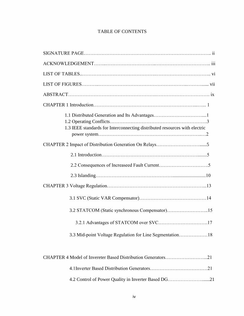
TABLE OF CONTENTS

SIGNATURE PAGE…………………………………………………………………….. ii

ACKNOWLEDGEMENT……..………………………….…………………………….. iii

LIST OF TABLES..……………………………………….…………………………….. vi

LIST OF FIGURES………..………………………………………………..………...... vii

ABSTRACT……………………………………………….……………………………. ix

CHAPTER 1 Introduction………………………………………………………...…... 1

1.1 Distributed Generation and Its Advantages…………………………....1

1.2 Operating Conflicts…………………………………………………….3

1.3 IEEE standards for Interconnecting distributed resources with electric

power system………………………………………………………..…2

CHAPTER 2 Impact of Distribution Generation On Relays………………………......5

2.1 Introduction……………………………………………………........5

2.2 Consequences of Increaseed Fault Current………………………….5

2.3 Islanding…………………………………………............................10

CHAPTER 3 Voltage Regulation……………………………………………………...13

3.1 SVC (Static VAR Compensator)……………………………………14

3.2 STATCOM (Static synchronous Compensator)……………………..15

3.2.1 Advantages of STATCOM over SVC………………………….17

3.3 Mid-point Voltage Regulation for Line Segmentation………………18

CHAPTER 4 Model of Invereter Based Distribution Generators……………………...21

4.1Inverter Based Distribution Generators………………………………21

4.2 Control of Power Quality in Inverter Based DG………………….......21

v

4.3 ABC to DQO Transformation……………………………………….25

4.3.1 Advantages of DQO Transformation………………………….26

CHAPTER 5 Simulation and Output Plots……………………………………………..27

CHAPTER 6 Conclusion………………………………………………………………...41

REFERENCE..…………………………………………………………………………..42

APPENDIX ……………………………………………………………………………..43

vi

LIST OF TABLES

Table 1: Branch Data 15………………………………………...30

Table 2: Bus Data, Base Case, No DG…………………………..31

Table 3: Generator Data………………………………………....32

Table 4: Output Bus Voltage…………………………………….33

Table5: Output Brach Losses……………………………………34

vii

LIST OF FIGURES

Figure 1: Protective relay for small sample distribution system with DG’s

…………………………………………………………………………………………..6

Figure 2: Fuse with current characteristics in the sample system with no DG

………………………………………………………………………………………….6

Figure 3: Fuse with current characteristics in the sample system with DG……..……7

Figure4: Fuse with current characterictics in the sample system special

case…………………………………………………………………………………….8

Figure 5: SVC…………………………………………………………………………15

Figure 6: STATCOM…………………………………..................................................16

Figure 7: V-I characteristics of STATCOM…………………………………………....17

Figure 8:Mid-point Voltage Regulation of Line Segment..............................................18

Figure 9: Phasor Diagram showing Mid-point Voltage regulation……………………..19

Figure 10: Plot Showing Relationship between active and reactive power……………..20

Figure 11: Grid System with DG………………………………………………………..22

Figure 12: Control Model of a DG with inverter………………………………………..23

Figure 13: Amplitude controller of an inverter………………………………………….24

Figure 14: Phase controller of an invereter……………………………………………..25

Figure 15: BUS 3 with FACT device in normal operating mode……………………….27

Figure 16: IEEE 14 bus test system bus diagram (case 1: no dg at buses 2, 6 and

8)……………………………………………………….………………………………..28

viii

Figure 17: IEEE 14 bus test system bus diagram (case 2: dg connected at bus

8)……………………………………………………………………………………….28

Figure 18: IEEE 14 bus test system bus diagram (case 3: dg connected at bus 6 and

8)………………………………………………………………………………………..29

Figure 19: IEEE 14 bus test system bus diagram (case 4: dg connected at buses 2, 6 and

8)………………………………………………………………………………………..29

Figure 20: Plot of Bus number vs. Bus voltage for no generator case…………............35

Figure 21: Plot of Bus number vs. Bus voltage for one generator case………………..35

Figure 22: Plot of Bus number vs. Bus voltage for 2 generator case………………….. 36

Figure 23: Plot of Bus number vs. Bus voltage for 3 generator case………………..….36

Figure 24: Plot of Branch vs. Loss P (MW) for no generator case………………….......37

Figure 25: Plot of Branch vs. Loss Q (MVAR) for no generator case………………….37

Figure 26: Plot of Branch vs. Loss P (MW) for 1 generator case…………………...….38

Figure.27: Plot of Branch vs. Loss Q (MVAR) for 1 generator case…………………..38

Figure 28: Plot of Branch vs. Loss P (MW) for 2 generator case ……………………....39

Figure 29 Plot of Branch vs. Loss Q (MVAR) for 2 generator case………………….. 39

ix

Figure 30: Plot of Branch vs. Loss P (MW) for 3 generator case ……………………40

Figure 31: Plot of Branch vs. Loss Q (MVAR) for 3 generator case…………………40

x

ABSTRACT

POWER FLOW ANALYSIS AND VOLTAGE REGULATION USING PSS/E-FACTS

By

Ajay Jose

Masters of Science in Electrical Engineering

The consequences and limitations of using distributed generation in power systems is

presented in this paper. Increased system fault currents due to installation of DG and its

effects are discussed. Various IEEE standards for the interconnection of distributed

resources with electric power system are also discussed. It provides requirements relevant

to the performance, operation, testing, safety considerations, and maintenance of this

interconnection. In order to analyze the effects from the increase of fault current due to

the installation of inverter based DGs, model of these DGs are studied. Mat power and

PSS/E are used for analysis and simulation.

1

CHAPTER 1

INTRODUCTION

1.1 INTRODUCTION:-

Distributed Generation is defined as “Electric generation facilities connected to an area Electric

Power System (EPS) operator through a Point of Common Coupling (PCC), a subset of

Distributed Resources.”

Since the 1990s, reciprocating engines and gas turbines have been rapidly placed into

service. Perhaps this deployment is a result of problems in dealing with transmission issues, and

problems in siting conventional generation, but for whatever reasons, protection engineers as

well as transmission and distribution engineers have to increasingly deal with problems related to

the added DG in the power systems.

The emergence of small and medium size DG arises from two major necessities:

Inadequacy of efficient power production.

Requirement of high reliability from industrial or commercial customers with a very high

value product.

Distributed generation can appear in different forms, both renewable and non-renewable.

Renewable technologies include fuel cells, wind turbines, solar cells, and geothermal.

Nonrenewable technologies include combined cycles, cogeneration, combustion turbine and

microturbines.

Increasing of non-utility generators rapidly increase consideration of effects of distributed

generation to the grid.

Advantages of Installing DG:-

Installing DG at a customer site enhances power quality by mitigating the voltage sag

during a fault.

Most faults on a power system are temporary, like arcing from overhead line to ground or

between phase conductors. These temporary faults on a distribution system should be detected

and cleared by protection relays and reclosers. During the period of fault, the voltage in the

distribution system drops. This phenomenon is called “voltage sag.” The magnitude of the sag

depends on the line impedance from substation to the fault location. Locally installed distributed

2

generation at a customer site can provide voltage support during fault in the utility transmission

system and improve the voltage sag performance.

DG improves the owner reliability considerably as a typical backup generator can be

started up within 2 minutes.

1.2 Operating Conflicts:-

The installation of DG in significant capacity will result in some conflicts with the operation of

the system.

If there is a high penetration of DGs, the conventional utility supply may not be able to

serve the load when the DGs drop off-line.

Installing a small or medium DG may not have a significant impact on the power quality

indices at the feeder level. The load should be disconnected from the supply feeder after a

specific period of time. The DG, after this disconnection, will have no impact on the

supply feeder. The DG has a local impact. The local load may be served properly, but

others on the common feeder will not experience improvement in voltage regulation.

1.3 IEEE Standards for interconnecting distributed resources with electric power system:-

IEEE Standard 1547

This standard provides the specifications and requirements for interconnection of distributed

resources with area electric power system (EPS). According to this standard, DR is defined as

sources of electric power including both generators and energy storage technologies. DG is the

electric generation facility which is a subset of distributed resources.

The requirements for interconnection of DR under normal conditions specified in the IEEE

Standard 1547 are:

The voltage regulation of the system after installing DG is + 5 % on a 120 volt base at the

service entrance (billing meter)

The DR unit should not cause the voltage fluctuation at the PCC higher than + 5 % of the

prevailing voltage level of the local EPS

3

The network equipment loading and interrupting capability (IC) of protection equipment,

such as fuse and CB should not be exceeded

The grounding of the DR should not because overvoltage’s that exceed the rating of the

equipment in local EPS.

The requirements for interconnection of DR under abnormal conditions are:

The DR unit should not energize to the area EPS when the area EPS is out of service

The DR unit should not cause the wrong operation of the interconnection system due to

electromagnetic interference

The interconnection system should be able to withstand the voltage and current surges

The DR unit should cease to energize the area EPS within the specific clearing time due

to abnormal voltage and frequency

The DR unit should not cause power quality problems higher than specified tolerable

limits, such as DG harmonic current injection, flicker and resulting harmonic voltages.

In case the system frequency is lower than 57 Hz, the DR unit should cease to energize to the

area EPS within 16 ms. When a fault is detected, the DGs must be disconnected from the electric

utility company supply and the DG should pick up the local load. The disconnection is needed

because

A fault close to the DG in the supply system must be interrupted

The local DG cannot support the power demands of the distribution system apart from the

local load.

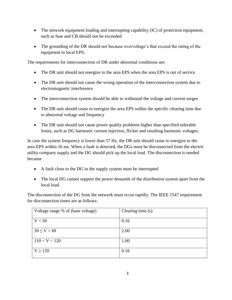
The disconnection of the DG from the network must occur rapidly. The IEEE 1547 requirement

for disconnection times are as follows:

Voltage range % of (base voltage) Clearing time (s)

V < 50 0.16

50 ≤ V < 88 2.00

110 < V < 120 1.00

V ≥ 120 0.16

4

Table showing IEEE 1547 requirement for disconnection time.

Most utilities utilize a common set of rules to interconnect the DG to power system like,

Exchange the project information between utility and customer

Technical analysis by the utility to evaluate the impact of DGs

Inspection of interconnection and protective equipment by the utility.

5

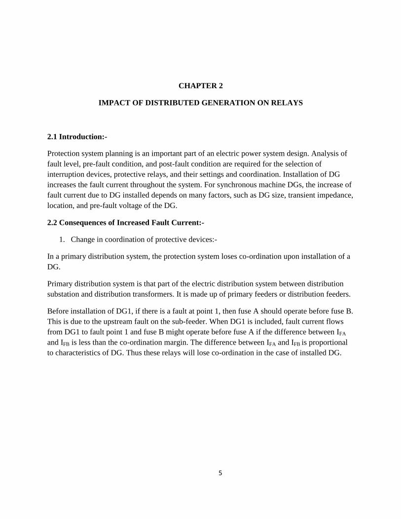
CHAPTER 2

IMPACT OF DISTRIBUTED GENERATION ON RELAYS

2.1 Introduction:-

Protection system planning is an important part of an electric power system design. Analysis of

fault level, pre-fault condition, and post-fault condition are required for the selection of

interruption devices, protective relays, and their settings and coordination. Installation of DG

increases the fault current throughout the system. For synchronous machine DGs, the increase of

fault current due to DG installed depends on many factors, such as DG size, transient impedance,

location, and pre-fault voltage of the DG.

2.2 Consequences of Increased Fault Current:-

1. Change in coordination of protective devices:-

In a primary distribution system, the protection system loses co-ordination upon installation of a

DG.

Primary distribution system is that part of the electric distribution system between distribution

substation and distribution transformers. It is made up of primary feeders or distribution feeders.

Before installation of DG1, if there is a fault at point 1, then fuse A should operate before fuse B.

This is due to the upstream fault on the sub-feeder. When DG1 is included, fault current flows

from DG1 to fault point 1 and fuse B might operate before fuse A if the difference between IFA

and IFB is less than the co-ordination margin. The difference between IFA and IFB is proportional

to characteristics of DG. Thus these relays will lose co-ordination in the case of installed DG.

6

Figure 1: The reach of a protective relay for a small sample distribution system with DGs

(Fig from “Fault Current Issues for market driven power systems with distributed generation”,

IEEE 2009)

MM: Minimum melting TC: Total clearing

Figure 2: Time-current characteristics of the fuse in the sample system of Fig. 1

(Before installation of DG)

7


IEEE)

Before installation of the DG, the current flowing through fuse A would be greater than the

current flowing through fuse B. For this case, from the curve we get that the current flowing

through fuse A is 103.5 A and this is in 8 seconds, and the current flowing through fuse B is

102.8 A and this is in say 400 seconds. So because of this difference in time (320 seconds), fuse

A would operate before fuse B.



(After installation of DG)


IEEE 2009)

After installation of the DG, suppose that the current flowing through fuse B is greater than the

current flowing through fuse B. For this case, from the curve we get that the current flowing

through fuse B is 103.5 A and this is in 0.03 seconds, and the current flowing through fuse A is

8

103.2 A and this is in say 1000 seconds. So because of this difference in time (999.97 seconds),

fuse B would operate before fuse A.




IEEE 2009)

The coordination margin is the difference in current between the minimum melting time of fuse

A and the total clearing time of fuse B, at a given time. Thus, if the difference between IFA and

IFB is less than the coordination margin, then fuse B would operate before fuse A.

2. Nuisance Trip:-

For a fault on any feeder other than DG3, breaker CB may also trip due to fault current flowing

from DG3 to fault point. This can be prevented by using directional relay instead of overcurrent

relay.

9

3. Recloser Setting:-

A DG should detect the fault and disconnect from the system within the recloser interval and

leave some duration for fault to clear. Otherwise, it may cause a persistent fault rather than

temporary one.

4. Safety:-

Installation of DG increases the fault current. If this fault current is higher than the interrupting

capability of circuit breakers, it may cause damage to personnel and equipment.

5. Changing the reach of protective relays:-

Reach is the term describing how far down a feeder a protective device is able to sense the fault.

Consider a resistive fault at fault point 2. If there is a DG2 present between the fault points, it

might cause a lower fault current to be seen by the protective relay. This has the following

impacts:

The fault is undetected, allowing it to burn indefinitely until the fault resistance

decreases.

The recloser response is slowed, which allows more damage to occur or fuse

saving to fail.

6. If a utility company worker is not aware that there is a DG running in the system, they

might be injured from electric shock, while working on lines or with other equipment.

7. If a DG is the only supply to the distribution system, after the DG is disconnected from

the primary distribution supply, voltage waveform from DG’s may fluctuate and may not

10

meet voltage regulation standards. The DG equipment may be damaged due to

overloading.

2.3 Islanding:

Even if the network with connected inverters is disconnected from the main utility,they tend to

energize the local load regardless of the utility.It can cause potential hazards and therefore

protection from islanding is essential.

There are two types of protection schemes for islanding: passive and active methods. Over

current, over and under voltage, over and under frequency all comes under passive protection

schemes. But in case of a DG due to the formation of non-detection zones (NDZ), passive

protection schemes alone cannot protect the utility form islanding. Therefore, we incorporate

active anti-islanding scheme for protection.

Since this paper is focused on DG’s, active islanding methods based on LOG or Loss of Grid

Protection is implemented.

LOG protection helps to check if the DGs are still in connection with utility even if there is no

power source connected. Thus by identifying the above condition the circuit breaker between the

DG and the utility network can be disconnected immediately and thus can enable an easy

restoration of the supply and also avoid any dissimilarity between the two systems thereby

avoiding any damage to the systems.

There are three requirements for this LOG protection Scheme:

1. The relay should have a time limit of thirty seconds to operate with the outage of power.

2. The DG’s should maintain the system voltage and frequency within the specified limits.

3. It should also prevent any out of synchronism reclosure.

11

Active Schemes:

1. Reactive Power Export Error Detection

In this method the relay interfaces with the DG control system and forces it to generate a level of

reactive power flow in PCC (point of common coupling).It can last till the supply is ON. The

operation of the relay is triggered as soon as a differernce in the set value and actual value is

seen.Any mis-operations are controlled by increasing the timesetting to a longer duration. This is

a comparatively slow protection scheme as the operating time is from 2 to 5 seconds.

2. EPS- Fault Level Monitoring.

This scheme is a faster acting protection technique than the previous one.Source impedance of

the EPS near to point of common coupling triggers the protection in this case.The signals from

the fault and actual value are compared and the realy is triggered accordingly.This protection is

faster than the prevviuos scheme and is beingf widely used in the EPS. It keeps a track of the

differences in the EPS and distributed generators and therefore this type of monitoring is

considered to be not very precise in the reading.

Passive Schemes:

1. Under/Over Voltage Under/Over Frequency

This type of scheme is used in smaller distributed generators and hence it is not widely used.

This scheme may be compromised due to several conditions and are rarely used in modern EPS

for protection.

2. Rate of change of Frequency (ROCOF)

In this scheme the ROCOF relays, the voltage waveform is looked upon and the frequencies are

noted.Once a change in the frequency with that of a preset value is detected the circuit breaker

trips accordingly. The relay operates only of there is fluctuations associated with the LOG and

DG’s and not if there is any fluctuations in the utility level.

Small and medium sized distributed generators can be protected using this scheme.

12

3. Phase displacement Monitoring

ROCOF and phase displacement monitoring goes hand in hand.It functions depending on the

phase displacement in the waveform (voltage).These relays are quick to respond to any changes

in the system and have an operating time of about 50ms.

13

CHAPTER 3

VOLTGE REGULATION

Voltage regulation is very important in any power system in order to maintain the voltage and

minimize the losses.” Voltage regulation is the change in voltage at the receiving end of the line

when the load varies from no-load to a specified full load at a specified power factor while

sending –end voltage is held constant.” (Power System Analysis and Design by J. Duncan

Glover)

Percent regulation –

Where | is the magnitude of load voltage at no load and | is the magnitude of at

full load with | constant.

FACTS-(Flexible alternating current transmission systems):

IEEE defines facts as “a power electronic based system and other static equipment that provide

control of one or more AC transmission system parameters to enhance controllability and

increase power transfer capability”.

There are several types of FACTS controllers, most commonly used are as follows:

1. Series Controllers.

2. Shunt Controllers.

3. Combined series-series.

4. Combined series-shunt.

Series controller refers to any variable impedance or variable source that injects voltage in series

with the line. It’s a very powerful active controller and it helps in improving the transient

stability of the power system. FACTS works as a controllable voltage source.

Shunt compensation refers to any variable impedance or source that injects current in to the line

and helps improve dynamic stability. FACTS works as a controllable current source.

Combined series-series controllers could be a combination of separate series controllers which

are controlled in a coordinated manner or it could be a unified controller.

Combined series-shunt controllers are either controlled in a coordinated manner or a unified

Power Flow Controller with series and shunt elements.

14

D-FACTS are very similar to the FACTS with the only difference that these devices are used in

distribution systems. They are custom power compensating shunt comptrollers with the main

purpose of voltage regulation, load compensation and voltage profile improvement.

Today distribution power systems are facing severe problems mainly because of the voltage drop

along the feeders due to real and reactive power flow. D-SVC and D-STATCOM are the most

commonly used D-FACTS for compensating the voltage drop. A lot of research is going on with

D-FACTS so as to improve its functionality.

3.1 SVC (Static VAR Compensator)

The SVC is a solid-state is reactive power compensation device used for improving power

quality and voltage control.The SVC installed in power system at suitable locations can improve

the transfer capability, mitigate power oscillations and help improve the voltage profile.

The benefits of installing SVC’s in distribution system are as follows:

1. Stabilized voltage at the receiving end of long lines.

2. Reducing losses by reducing reactive power consumption.

3. Enables better use of equipment’s.

4. Reduced flicker and harmonic distortion.

5. Reduced voltage fluctuations.

15

Figure 5: from “SVC Static Var Compensator insurance for improved grid system stability and

reliability” by ABB.

A reactor and thyristor valve are incorporated in each single-phase branch. Power is changed by

controlling the current through the reactor via the thyristor valve. The on-state interval is

controlled by delaying triggering of the thyristor valve relative to the natural zero current

crossing.

A thyristor controlled reactor (TCR) is used in combination with a fixed capacitor (FC) when

reactive power generation or alternatively, absorption and generation are required. This is often

the optimum solution for sub-transmission and distribution.

3.2 STATCOM (Static synchronous Compensator):

STATCOM is a static synchronous generator operated as a shunt-connected static var

compensator whose capacitive or inductive output current can be controlled independent of the

ac system voltage. The STATCOM like its counterpart the SVC, controls transmission voltage

by reactive shunt compensation. STATCOM can be designed to be an active filter to absorb

system harmonics.

16

Figure 6: from “Investigation of different load changes in wind farm by using FACTS devices by

Ali Oztruz and M.Kenan Dosogulu”

The STATCOM consists of VSC (Voltage Synchronous converter), coupling transformer that

generates the voltage wave comparing to the one of the electric system. The voltage support for

the VSC in most cases is given by the small dc source like a battery. The GTO (Gate turn off)

converter generates a voltage that is stepped up by the transformer. The transformer helps in

building up a sine wave both in phase and magnitude. If the number of firing pulses for the GTO

is increased the harmonics can be reduced further.

17

Figure7: from “Investigation of different load changes in wind farm by using FACTS devices by

Ali Oztruz and M.Kenan Dosogulu”

The figure above shows the V-I characteristics of STATCOM. The STATCOM smoothly and

continuously controls voltage from V1 to V2. However, if the system voltage exceeds a low-

voltage (V1) or high-voltage limit (V2), the STATCOM acts as a constant current source by

controlling the converter voltage (Vi) appropriately.

3.2.1 Advantages of STATCOM over SVC:

1. A STATCOM has a step response of 8ms to 30ms which helps with compensation of

negative phase current and with the reduction of voltage flicker.

2. Active power control is possible with a STATCOM with optional energy storage on dc

circuit.

3. The STATCOM has a smaller installation space due to no capacitors or reactors required

to generate Mvar, minimal or no filtering, and the availability of high capacity power

semiconductor devices. Designs of systems of equal dynamic ranges have shown the

STATCOM to be as much as 1/3 the area and 1/5 the volume of an SVC.

4. A modular design of the STATCOM allows for high availability (i.e., one or more

modules of the STATCOM can be out-of-service without the loss of the entire

compensation system).

18

3.3 Mid-Point Voltage Regulation for Line Segmentation:

Reactive compensation is used to control the voltage profile along the line as well as to increase

the steady state transmittable power along the line. Its helps to change the natural electrical

characteristics of the transmission line to make it more compatible with the prevailing load

demands. Shunt connected, fixed or mechanically switched reactors are applied to minimize line

over voltage under light load conditions, and shunt connected, fixed or mechanically switched

capacitors are applied to maintain voltage levels under heavy load conditions.

Var compensation is used for the voltage regulation at the midpoint of the transmission line and

at the end of the line to prevent voltage instability as well as for dynamic voltage control to

increase transient stability and damp power oscillations.

The figure below shows a two-bus transmission model in which an ideal var compensator is

shunt connected at the midpoint of the transmission line. The line is represented by the series line

inductance. The compensator is represented by a sinusoidal ac voltage source in-phase with the

midpoint voltage, Vm, and with an amplitude identical to that of the sending-end voltages

(Vm=Vs=Vr=V).

Figure 8: from “Understanding FACTS concepts and technology of Flexible AC Transmission

Systems by Narain G.Hingorani, Laszlo Gyugyi.”

The above model is divided in to two segments the first segment with an impedance of X/2,

carries power from the sending end to the midpoint, and the second segment with an impedance

of X/2 carries power from the midpoint to the receiving end.

19

The Phasor diagram shows the relationship between voltages Vs, Vr, Vm, Vsm, Vrm and line

segment currents Ism and Imr. Only the reactive power with the transmission line is being

exchanged by the var compensator.



For a loss less system the real power is the same at each terminal of the line. It can be

derived from the phasor diagram as:

,

From the above equations we can get the transmitted power to be:

Similarly we can get the reactive power as:

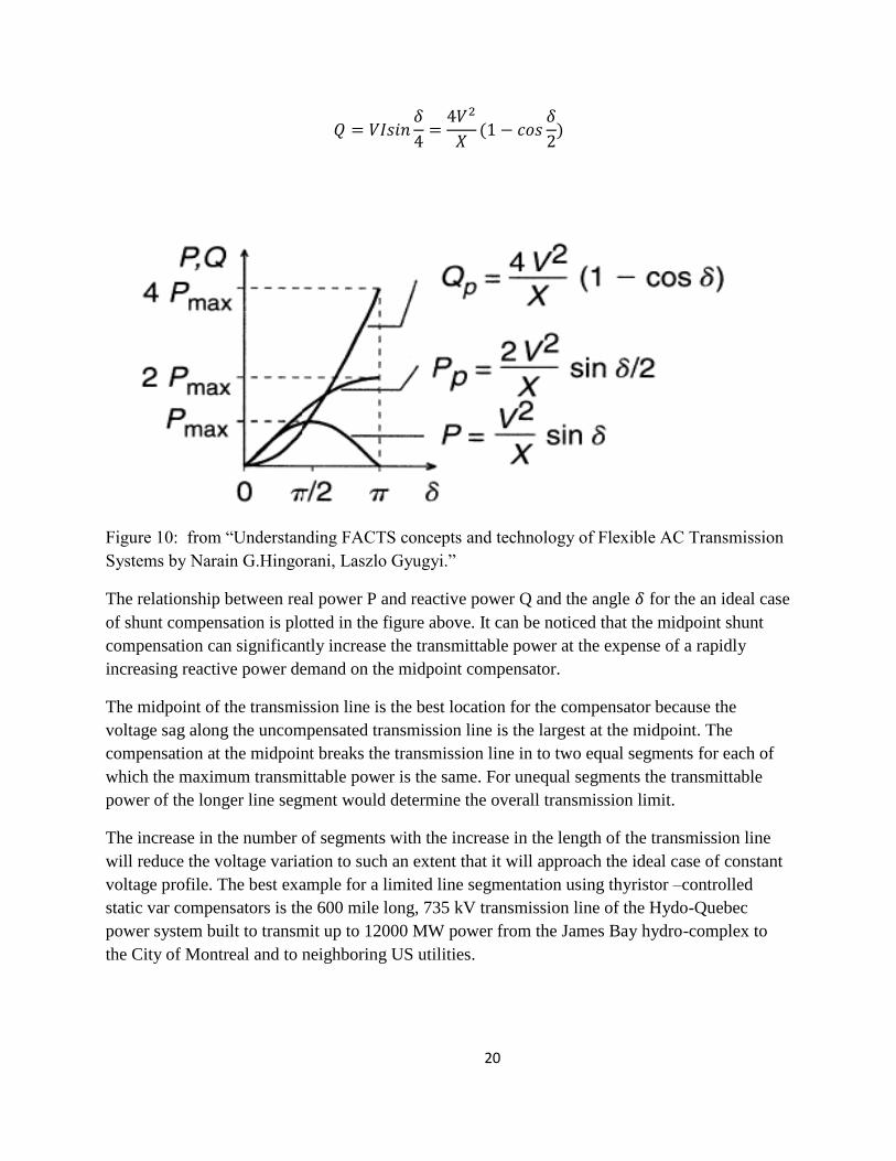
20



The relationship between real power P and reactive power Q and the angle for the an ideal case

of shunt compensation is plotted in the figure above. It can be noticed that the midpoint shunt

compensation can significantly increase the transmittable power at the expense of a rapidly

increasing reactive power demand on the midpoint compensator.

The midpoint of the transmission line is the best location for the compensator because the

voltage sag along the uncompensated transmission line is the largest at the midpoint. The

compensation at the midpoint breaks the transmission line in to two equal segments for each of

which the maximum transmittable power is the same. For unequal segments the transmittable

power of the longer line segment would determine the overall transmission limit.

The increase in the number of segments with the increase in the length of the transmission line

will reduce the voltage variation to such an extent that it will approach the ideal case of constant

voltage profile. The best example for a limited line segmentation using thyristor –controlled

static var compensators is the 600 mile long, 735 kV transmission line of the Hydo-Quebec

power system built to transmit up to 12000 MW power from the James Bay hydro-complex to

the City of Montreal and to neighboring US utilities.

21

CHAPTER 4

MODEL OF INVERTER BASED DISTRIBUTION GENERATORS

4.1 Inverter Based Generation Sources:-

Generation resources are traditionally synchronous generators, and modeling of these machines

is well known. Unlike conventional sources, power generated in fuel cells, solar sources and

some micro turbines are DC. In the case of these resources, an inverter is needed to interface

with the AC system network. Also, recent developments in the operation of power systems have

suggested that inverter based generation sources may be used for synchronous machines. That is,

the synchronous generator is isolated from the AC system through an AC / AC converter in order

to isolate the dynamics of the network from the local synchronous generator. Whatever the

motivation, it is appropriate to examine inverter based generation sources and their impact on

fault response in power systems.

Pulse Width Modulation (PWM) is used as the base technology for the inverters. For the model

of the inverter based DG, it is assumed that the input voltage from DC sources to the PWM

inverter are regulated by using DC/DC converters and chopper circuits.

4.2 Control of Power Quality in Inverter Based Distribution Generators:-

Inverter based DGs operate as controlled voltage sources connected to the grid system through a

step up transformer. The step up transformer with delta – delta connection (4 kV/12.47 kV)

eliminates the zero sequence components from inverter to the grid.

22

Figure 11: Inverter Based DG connecting to a Grid System (fig. from “Fault Current

Contribution from Synchronous Machine and Inverter Based Distributed Generators”, IEEE

2007)

Consider the active power of an inverter based DG, denominated as PDG. Let PDG be at the output

of the inverter. The active power PDG is an average of the instantaneous power PDG(t). The

average is taken over at least one cycle, but, more likely, taken over a time period measured in

seconds. The active power output of the inverter based DG could be estimated as,

PDG =

(Equation 1)

Where V1, V2 are the voltage magnitudes at the primary and secondary sides of the step up

transformer and δ is the difference of phase angle between V1 and V2.

The above equation is a simplistic representation of PDG because:

Inverter losses are ignored

Inverter dynamics are ignored

Equation 1 is an elementary model based on lossless AC circuit theory, and no source

dynamics are modeled. For example, in a fuel cell, the DG source at the fuel cell

terminals may not be constant.

It is expected that the relatively long time dynamics of δ (t) are well modeled using Re{VI *}

because V and I are rms values averaged over at least one cycle. Figure 6 shows the control

23

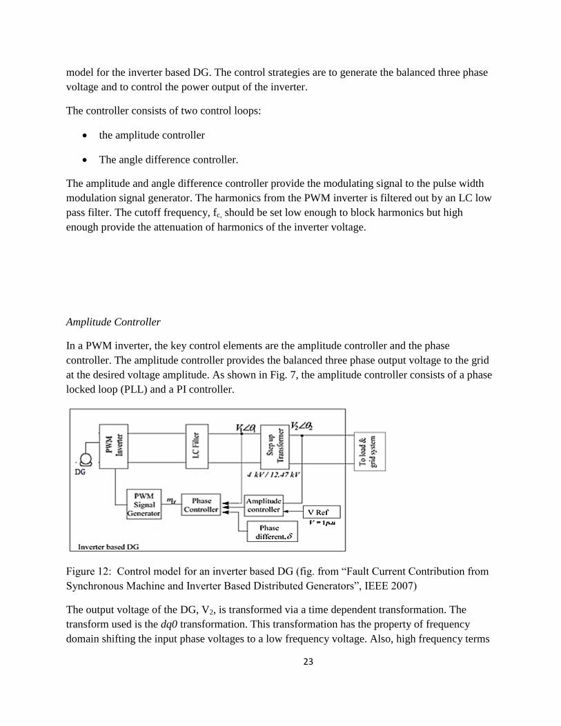
model for the inverter based DG. The control strategies are to generate the balanced three phase

voltage and to control the power output of the inverter.

The controller consists of two control loops:

the amplitude controller

The angle difference controller.

The amplitude and angle difference controller provide the modulating signal to the pulse width

modulation signal generator. The harmonics from the PWM inverter is filtered out by an LC low

pass filter. The cutoff frequency, fc, should be set low enough to block harmonics but high

enough provide the attenuation of harmonics of the inverter voltage.

Amplitude Controller

In a PWM inverter, the key control elements are the amplitude controller and the phase

controller. The amplitude controller provides the balanced three phase output voltage to the grid

at the desired voltage amplitude. As shown in Fig. 7, the amplitude controller consists of a phase

locked loop (PLL) and a PI controller.

Figure 12: Control model for an inverter based DG (fig. from “Fault Current Contribution from

Synchronous Machine and Inverter Based Distributed Generators”, IEEE 2007)

The output voltage of the DG, V2, is transformed via a time dependent transformation. The

transform used is the dq0 transformation. This transformation has the property of frequency

domain shifting the input phase voltages to a low frequency voltage. Also, high frequency terms

24

occur. It is assumed that the high frequency terms that occur in the dq0 transformed variables are

filtered out. The control is performed in dq0 reference frame because of the advantage for the

instantaneous voltage angle calculation.

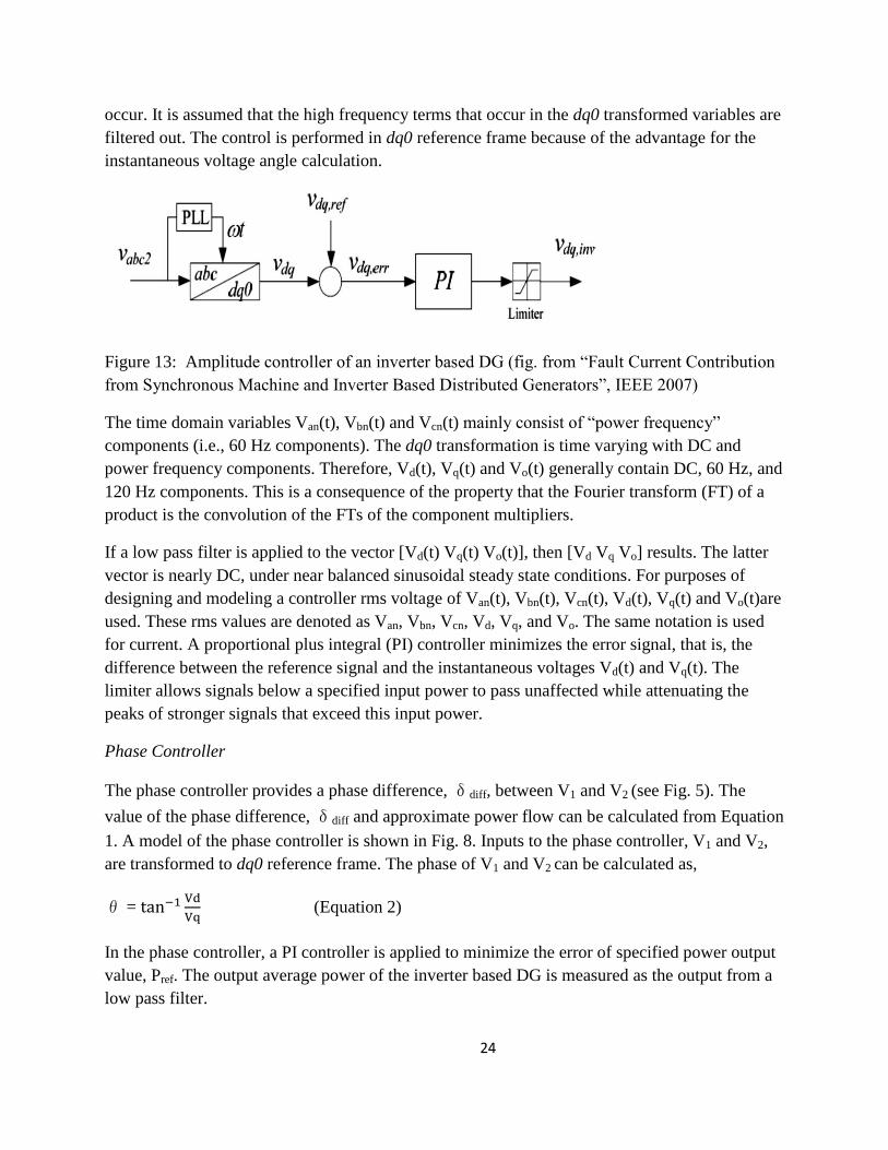
Figure 13: Amplitude controller of an inverter based DG (fig. from “Fault Current Contribution

from Synchronous Machine and Inverter Based Distributed Generators”, IEEE 2007)

The time domain variables Van(t), Vbn(t) and Vcn(t) mainly consist of “power frequency”

components (i.e., 60 Hz components). The dq0 transformation is time varying with DC and

power frequency components. Therefore, Vd(t), Vq(t) and Vo(t) generally contain DC, 60 Hz, and

120 Hz components. This is a consequence of the property that the Fourier transform (FT) of a

product is the convolution of the FTs of the component multipliers.

If a low pass filter is applied to the vector [Vd(t) Vq(t) Vo(t)], then [Vd Vq Vo] results. The latter

vector is nearly DC, under near balanced sinusoidal steady state conditions. For purposes of

designing and modeling a controller rms voltage of Van(t), Vbn(t), Vcn(t), Vd(t), Vq(t) and Vo(t)are

used. These rms values are denoted as Van, Vbn, Vcn, Vd, Vq, and Vo. The same notation is used

for current. A proportional plus integral (PI) controller minimizes the error signal, that is, the

difference between the reference signal and the instantaneous voltages Vd(t) and Vq(t). The

limiter allows signals below a specified input power to pass unaffected while attenuating the

peaks of stronger signals that exceed this input power.

Phase Controller

The phase controller provides a phase difference, δdiff, between V1 and V2 (see Fig. 5). The

value of the phase difference, δdiff and approximate power flow can be calculated from Equation

1. A model of the phase controller is shown in Fig. 8. Inputs to the phase controller, V1 and V2,

are transformed to dq0 reference frame. The phase of V1 and V2 can be calculated as,

θ =

(Equation 2)

In the phase controller, a PI controller is applied to minimize the error of specified power output

value, Pref. The output average power of the inverter based DG is measured as the output from a

low pass filter.

25

The cut-off frequency of the low pass filter has to be set at the appropriate value to attenuate the

disturbance from measurement, but high enough to provide a good transient response of the

phase controller. The output of the PI controller is added to the phase of V1 and used to calculate

the required amplitude and phase of the modulating signal. The last step in the phase difference

controller is to transform the modulating signal back to the abc reference frame.

Figure 14: Phase controller of an inverter based DG (fig. from “Fault Current Contribution from

Synchronous Machine and Inverter Based Distributed Generators”, IEEE 2007)

4.3 ABC to DQO Transformation:

ABC transformation is the basis of other model representations. ABC increases the

computational burden due to presence of ac quantities varying with the rower frequency or

system frequency (50, 60 Hz).

[

]

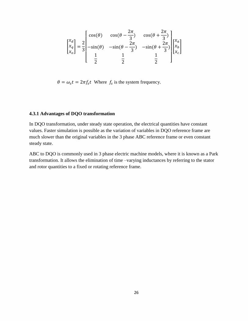
Park’s transformation or DQO (direct quadrature zero) is used for transforming ac terms to dc

terms for simplified calculations as there is no frequency term in dc. DQO representation is a

commonly used variable representation in power systems area.

26

[

]

[

]

[

]

Where is the system frequency.

4.3.1 Advantages of DQO transformation

In DQO transformation, under steady state operation, the electrical quantities have constant

values. Faster simulation is possible as the variation of variables in DQO reference frame are

much slower than the original variables in the 3 phase ABC reference frame or even constant

steady state.

ABC to DQO is commonly used in 3 phase electric machine models, where it is known as a Park

transformation. It allows the elimination of time –varying inductances by referring to the stator

and rotor quantities to a fixed or rotating reference frame.

27

CHAPTER 5

SIMULATION

Simulation of an IEEE 14 bus system is carried out using PSS/E software from SIEMENS. The

FACT device is connected to different buses depending on voltage regulation. The FACT device

is operated on two modes of operation: normal and blocked and the voltage is regulated

accordingly. The advantages and functionality of connecting a FACT device is thus understood

and studied.

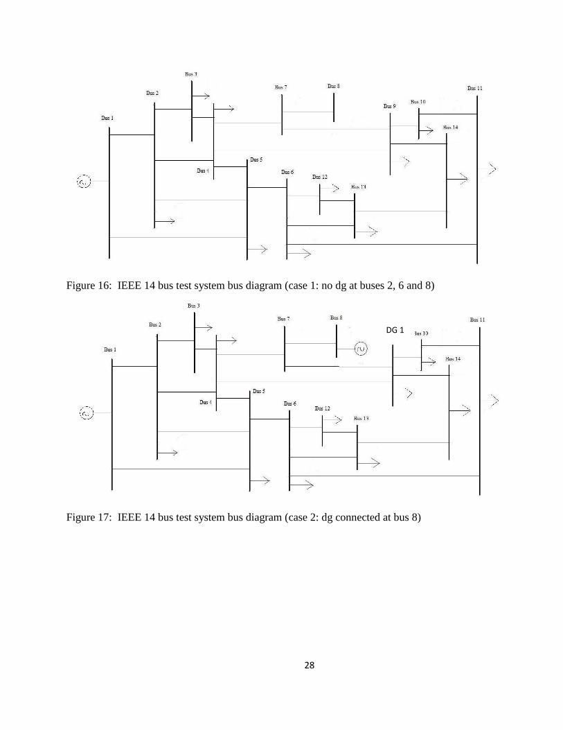
Simulation of a 14 bus test system is carried out in mat power. Mat power is a package of mat

lab M-files for solving power flow and optimal power flow problems. The 14 bus case is

modified for 4 different cases. Case 1: no Dg connected; Case 2: DG connected at bus 8; Case 3 :

DG connected at buses 6 and 8; Case 4 : DG connected at buses 2, 6 and 8. The power flow data

is given in the mat power M-file. The bus data, generator data, branch data, area data and the

generator cost data is specified in the mat power M-file.

Figure 15: Bus 3 with FACTS device in normal operating mode.

31

1.0345.0

Bus # 3 1 345.00

Type 1 Area 1 Zone 1

Voltage 1.00000PU 345.000KV

Angle (deg) -1.87

1 20.0

10.0

0.0

-8.4

21

1.0346.4

* 10.9

-2.6

-10.8

-1.5

41

1.0346.9

* -9.2

-0.1

9.2

-1.0

28

Figure 16: IEEE 14 bus test system bus diagram (case 1: no dg at buses 2, 6 and 8)

Figure 17: IEEE 14 bus test system bus diagram (case 2: dg connected at bus 8)

DG 1

29

Figure 18: IEEE 14 bus test system bus diagram (case 3: dg connected at bus 6 and 8)

Figure 19: IEEE 14 bus test system bus diagram (case 4: dg connected at buses 2, 6 and 8)

DG 1

DG 2

DG 1

DG 2

DG 3

30

From

bus#

To

bus#

R(pu) X(pu) B(pu) Transformer

turns ratio

Transformer

phase shift

angle

status

1 2 0.01938 0.05917 0.0528 0 0 1

1 5 0.05403 0.22304 0.0492 0 0 1

2 3 0.04699 0.19797 0.0438 0 0 1

2 4 0.05811 0.17632 0.034 0 0 1

2 5 0.05695 0.17388 0.0346 0 0 1

3 4 0.06701 0.17103 0.0128 0 0 1

4 5 0.01335 0.04211 0 0 0 1

4 7 0 0.20912 0 0.978 0 1

4 9 0 0.55618 0 0.969 0 1

5 6 0 0.25202 0 0.932 0 1

6 11 0.09498 0.1989 0 0 0 1

6 12 0.12291 0.25581 0 0 0 1

6 13 0.06615 0.13027 0 0 0 1

7 8 0 0.17615 0 0 0 1

7 9 0 0.11001 0 0 0 1

9 10 0.03181 0.0845 0 0 0 1

9 14 0.12711 0.27038 0 0 0 1

10 11 0.08205 0.19207 0 0 0 1

12 13 0.22092 0.19988 0 0 0 1

13 14 0.17093 0.34802 0 0 0 1

Table 1. Branch Data

Table 1 show the branch data whose format is

1) fbus, from bus number

2) tbus, to bus number

3) r, resistance (p.u.)

4) x, reactance (p.u.)

5) b, total line charging susceptance (p.u.)

6) rate A, MVA rating A (long term rating)

7) rate B, MVA rating B (short term rating)

31

8) rate C, MVA rating C (emergency rating)

9) ratio, transformer off nominal turns ratio

10) angle, transformer phase shift angle (degrees)

11) status, initial branch status, 1 – in service, 0 – out of service

Bus# Busy

type

Pd(MW) Qd(MVAR) Area# Vmag Vangle Base

KV

zone Vmax

(pu)

Vmin

(pu)

1 3 0 0 1 1.06 0 345 1 1.06 0.94

2 2 21.7 12.7 1 1.045 -4.98 345 1 1.06 0.94

3 2 94.2 19 1 1.01 -12.72 345 1 1.06 0.94

4 1 47.8 -3.9 1 1.019 -10.33 345 1 1.06 0.94

5 1 7.6 1.6 1 1.02 -8.78 345 1 1.06 0.94

6 2 11.2 7.5 1 1.07 -14.22 345 1 1.06 0.94

7 1 0 0 1 1.062 -13.37 345 1 1.06 0.94

8 2 0 0 1 1.09 -13.36 345 1 1.06 0.94

9 1 29.5 16.6 1 1.056 -14.94 345 1 1.06 0.94

10 1 9 5.8 1 1.051 -15.1 345 1 1.06 0.94

11 1 3.5 1.8 1 1.057 -14.79 345 1 1.06 0.94

12 1 6.1 1.6 1 1.055 -15.07 345 1 1.06 0.94

13 1 13.5 5.8 1 1.05 -15.16 345 1 1.06 0.94

14 1 14.9 5 1 1.036 -16.04 345 1 1.06 0.94

Table 2. Bus Data, Base Case, No DG

Table 2 shows the bus data whose format is

1) Bus number

2) Bus type

PQ bus = 1

PV bus = 2

Reference bus = 3

Isolated bus = 4

3) Pd, real power demand (MW)

32

4) Qd, reactive power demand (MVAR)

5) Gs, shunt conductance (MW (demanded) at V = 1.0 p.u.)

6) Bs, shunt susceptance (MVAR (injected) at V = 1.0 p.u.)

7) Area number

8) Vm, voltage magnitude (p.u.)

9) Va, voltage angle (degrees)

10) baseKV, base voltage (kv)

11) zone, loss zone

12) maxVm, maximum voltage magnitude (p.u.)

13) minVm, minimum voltage magnitude (p.u.)

Bus# Pg

(MW)

Qg

(MVAR)

Qmax

(MVAR)

Vg

(pu)

Base

(MVA)

status P (MW)

1 232.4 -16.9 10 1.06 100 1 332.4

2 40 42.4 50 1.045 100 1 140

6 40 42.4 50 1.07 100 1 140

8 40 42.4 50 1.09 100 1 140

Table 3. Generator data

Table 3 shows the generator data whose format is

1) bus number

2) Pg, real power output (MW)

3) Qg, reactive power output (MVAR)

4) Qmax, maximum reactive power output (MVAR)

5) Qmin, minimum reactive power output (MVAR)

6) Vg, voltage magnitude setpoint (p.u.)

33

7) mBase, total MVA base of this machine, defaults to baseMVA

8) status, > 0 – machine in service

<= 0 – machine out of service

9) P, maximum real power output (MW)

Simulation Results: - 4 cases: case1 (No DG), case2 (1 DG), case3 (2 DG’s), case4 (3 DG’s)

BUS# Vmag

(p.u)

Vangle

(deg)

Vmag

(p.u)

Vangle

(deg)

Vmag

(p.u)

Vangle

(deg)

Vmag

(p.u.)

Vangle

(deg)

case 1 (no DG

connected)

case 2 (DG

connected at

bus 8)

case 3 (DG

connected at buses

6 and 8)

case 4 (DG connected

at buses 2, 6 and 8)

1 1.06 0 1.06 0 1.06 0 1.06 0

2 0.986 -5.528 1.012 -4.779 1.023 -3.99 1.045 -3.135

3 0.91 -13.872 0.954 -11.955 0.971 -10.436 0.989 -9.416

4 0.935 -11.095 0.991 -9.027 1.011 -7.162 1.024 -6.282

5 0.946 -9.357 0.994 -7.684 1.016 -5.89 1.027 -5.095

6 0.953 -15.951 1.022 -12.324 1.07 -7.026 1.07 -6.15

7 0.942 -14.832 1.042 -9.424 1.057 -6.56 1.063 -5.724

8 0.942 -14.832 1.09 -5.868 1.09 -3.054 1.09 -2.238

9 0.937 -16.835 1.03 -11.978 1.051 -8.518 1.057 -7.679

10 0.932 -17.042 1.021 -12.351 1.047 -8.54 1.051 -7.696

11 0.938 -16.661 1.018 -12.482 1.055 -7.917 1.057 -7.061

12 0.936 -17.031 1.008 -13.164 1.055 -7.938 1.055 -7.06

13 0.931 -17.133 1.005 -13.19 1.049 -8.07 1.05 -7.2

14 0.914 -18.243 1.001 -13.573 1.032 -9.329 1.036 -8.472

Table 4. Output Bus Voltage

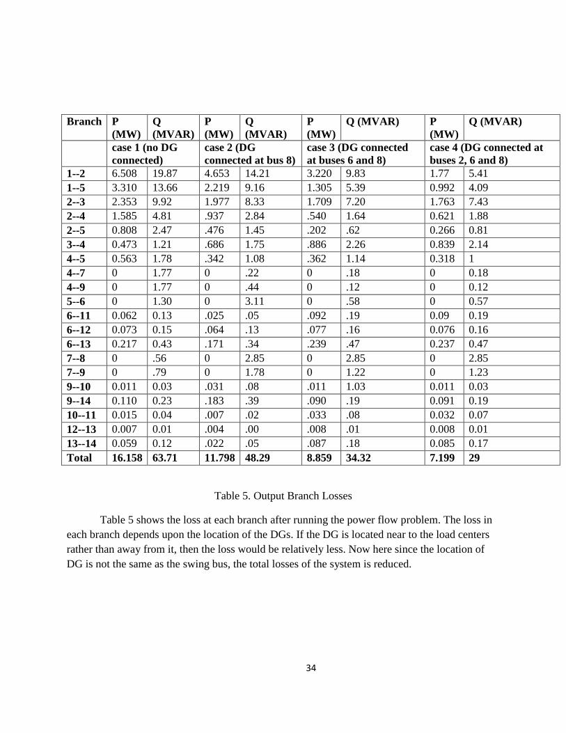
Table 4 shows the voltage magnitude at each bus after running the power flow problem. It can be

seen that in case 2, the voltage of bus 8 increases from 0.942 p.u. to 1.09 p.u. This is because of

the installation of DG at bus 8. Installation of DG provides reactive power support and hence

voltage support to the system. Consequently, the voltage at all the bus is increased with the

voltage support by generator at bus 8. Now in case 3, when Dg is installed at bus 6, then the

voltage at bus 6 is increased which was already raised by the installation of DG at bus 8.

Consequently, the voltage at other buses is also increased. And finally, in case 4, with the

installation of DG at bus 2, the voltage at bus 2 which was already increased by DG at bus 6 and

8, raises even more. And the voltage at other buses is also increased. This property of DG is

important for providing voltage support during a fault as the voltage of the system drops during

the fault. Thus DG mitigates voltage sag during a fault.

34

Branch P

(MW)

Q

(MVAR)

P

(MW)

Q

(MVAR)

P

(MW)

Q (MVAR) P

(MW)

Q (MVAR)

case 1 (no DG

connected)

case 2 (DG

connected at bus 8)

case 3 (DG connected

at buses 6 and 8)

case 4 (DG connected at

buses 2, 6 and 8)

1--2 6.508 19.87 4.653 14.21 3.220 9.83 1.77 5.41

1--5 3.310 13.66 2.219 9.16 1.305 5.39 0.992 4.09

2--3 2.353 9.92 1.977 8.33 1.709 7.20 1.763 7.43

2--4 1.585 4.81 .937 2.84 .540 1.64 0.621 1.88

2--5 0.808 2.47 .476 1.45 .202 .62 0.266 0.81

3--4 0.473 1.21 .686 1.75 .886 2.26 0.839 2.14

4--5 0.563 1.78 .342 1.08 .362 1.14 0.318 1

4--7 0 1.77 0 .22 0 .18 0 0.18

4--9 0 1.77 0 .44 0 .12 0 0.12

5--6 0 1.30 0 3.11 0 .58 0 0.57

6--11 0.062 0.13 .025 .05 .092 .19 0.09 0.19

6--12 0.073 0.15 .064 .13 .077 .16 0.076 0.16

6--13 0.217 0.43 .171 .34 .239 .47 0.237 0.47

7--8 0 .56 0 2.85 0 2.85 0 2.85

7--9 0 .79 0 1.78 0 1.22 0 1.23

9--10 0.011 0.03 .031 .08 .011 1.03 0.011 0.03

9--14 0.110 0.23 .183 .39 .090 .19 0.091 0.19

10--11 0.015 0.04 .007 .02 .033 .08 0.032 0.07

12--13 0.007 0.01 .004 .00 .008 .01 0.008 0.01

13--14 0.059 0.12 .022 .05 .087 .18 0.085 0.17

Total 16.158 63.71 11.798 48.29 8.859 34.32 7.199 29

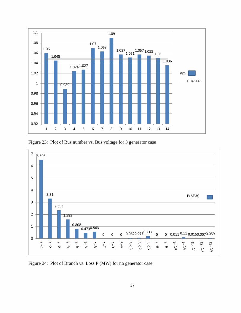
Table 5. Output Branch Losses

Table 5 shows the loss at each branch after running the power flow problem. The loss in

each branch depends upon the location of the DGs. If the DG is located near to the load centers

rather than away from it, then the loss would be relatively less. Now here since the location of

DG is not the same as the swing bus, the total losses of the system is reduced.

35

Output Plots:-

Figure 20: Plot of Bus number vs. Bus voltage for no generator case

1.06

0.986

0.91

0.935 0.946

0.953 0.942 0.942 0.937 0.932 0.938 0.936 0.931

0.914

0.8

0.85

0.9

0.95

1

1.05

1.1

1 2 3 4 5 6 7 8 9 10 11 12 13 14

.947286

Vm

36

Figure 21: Plot of Bus number vs. Bus voltage for one generator case

Figure 22: Plot of Bus number vs. Bus voltage for 2 generator case

1.06

1.012

0.954

0.991 0.994

1.022

1.042

1.09

1.03 1.021 1.018

1.008 1.005 1.001

0.85

0.9

0.95

1

1.05

1.1

1.15

1 2 3 4 5 6 7 8 9 10 11 12 13 14

1.017714

Vm

1.06

1.023

0.971

1.011 1.016

1.07

1.057

1.09

1.051 1.047 1.055 1.055

1.049

1.032

0.9

0.92

0.94

0.96

0.98

1

1.02

1.04

1.06

1.08

1.1

1 2 3 4 5 6 7 8 9 10 11 12 13 14

1.041929

Vm

37

Figure 23: Plot of Bus number vs. Bus voltage for 3 generator case

Figure 24: Plot of Branch vs. Loss P (MW) for no generator case

1.06

1.045

0.989

1.024 1.027

1.07 1.063

1.09

1.057 1.051

1.057 1.055 1.05

1.036

0.92

0.94

0.96

0.98

1

1.02

1.04

1.06

1.08

1.1

1 2 3 4 5 6 7 8 9 10 11 12 13 14

1.048143

Vm

6.508

3.31

2.353

1.585

0.808 0.473 0.563

0 0 0 0.062 0.073 0.217 0 0 0.011 0.11 0.015 0.007 0.059

0

1

2

3

4

5

6

7

P(MW)

38

Figure 25: Plot of Branch vs. Loss Q (MVAR) for no generator case

Figure 26: Plot of Branch vs. Loss P (MW) for 1 generator case

19.87

13.66

9.92

4.81

2.47 1.21

1.78 1.77 1.77 1.3 0.13 0.15 0.43 0.56 0.79

0.03 0.23 0.04 0.01 0.12 0

5

10

15

20

25

Q(MVAR)

4.653

2.219 1.977

0.937

0.476 0.686

0.342

0 0 0 0.025 0.064 0.171 0 0 0.031

0.183 0.007 0.004 0.022

0

0.5

1

1.5

2

2.5

3

3.5

4

4.5

5

P(MW)

39

Figure 27: Plot of Branch vs. Loss Q (MVAR) for 1 generator case


14.21

9.16 8.33

2.84

1.45 1.75 1.08

0.22 0.44

3.11

0.05 0.13 0.34

2.85 1.78

0.08 0.39 0.02 0 0.05 0

2

4

6

8

10

12

14

16

Q(MVAR)

3.22

1.305

1.709

0.54

0.202

0.886

0.362

0 0 0 0.092 0.077

0.239

0 0 0.011 0.09 0.033 0.008 0.087

0

0.5

1

1.5

2

2.5

3

3.5

P(MW)

40



9.83

5.39

7.2

1.64

0.62

2.26

1.14

0.18 0.12 0.58

0.19 0.16 0.47

2.85

1.22 1.03

0.19 0.08 0.01 0.18

0

2

4

6

8

10

12

Q(MVAR)

1.77

0.992

1.763

0.621

0.266

0.839

0.318

0 0 0 0.09 0.076

0.237

0 0 0.011 0.091

0.032 0.008 0.085

0

0.2

0.4

0.6

0.8

1

1.2

1.4

1.6

1.8

2

P (MW)

41


5.41

4.09

7.43

1.88

0.81

2.14

1

0.18 0.12 0.57

0.19 0.16 0.47

2.85

1.23

0.03 0.19 0.07 0.01 0.17

0

1

2

3

4

5

6

7

8

Q (MVAR)

42

CONCLUSION

The advantages and functionality of FACTS are understood and studied. The significance of

connecting FACTS in a power system is understood and analyzed using PSS/E software on a 14

bus test system. Mitigation of voltage sags due to loads by using FACTS is shown in the power

flow using PSS/E.

According to the demands of clean energy, consumer perceptions, high reliability and

power quality for sensitive loads the demand for distributed resources is gradually rising. The

benefits in the voltage support and loss reduction could be seen from the steady state simulations

mentioned above.

However as the penetration of DG increases, it should not be surprising that operating conflicts

would arise.

While DG may greatly improve the reliability for some DG owners, it can degrade the reliability

and power quality for some other customers on the feeder.

Distributed resources, such as fuel cells, micro turbines, solar cells and wind turbines, are mostly

based on electronic inverters. These inverters interface with the AC network result in changing

of the fault response throughout the system. In order to analyze the effects from the increase of

fault current due to the installation of inverter based DGs, model of these DGs is studied. The

model of inverter based DGs proposed is accomplished by applying the abc to dq0

transformation

Some problems with DG installation that I have studied in this paper are:

Change in coordination of protective devices

Nuisance trips

Recloser settings

Changing the reach of protective relays

For DG to be a success, one needs to understand these issues and provide practical solutions and

a path to get from where we are to the vision of a DG future.

43

REFERENCES

1. N. Nimpitiwan and G. T. Heydt, “Fault current contribution from synchronous machine and

inverter based distribution generators,” in Power Delivery, IEEE transactions, Jan 2007,

pp. 634 – 641.

2. N. Nimpitiwan and G. T. Heydt, “Fault current issues for market driven power systems with

distributed generation,” in Proc. North Amer. Power Symp., Moscow, Idaho, Aug. 2004, pp.

400–406.

3. R. C. Dugan and T. E. McDermott, “Operating conflicts for distributed generation on

distribution systems,” in Proc. Rural Electric Power Conf., 2001, pp. A3/1–A3/6.

4. R. C. Dugan and S. K. Price, “Issues for distributed generation in the US,” in Proc. IEEE

Power Eng. Soc. Winter Meeting, 2002, vol. 1, pp. 121–126.

5. IEEE Standard for Interconnecting Distributed Resources With Electric Power Systems, IEEE

Std. 1547-2003, Aug. 2003.

6. M. Prodanovic and T. C. Green, “Control of power quality in inverter based distributed

generation,” in Proc. IEEE Ind. Electron. Soc. Conf., 2002, vol. 2, pp. 1185–1189.

7. http://www.pserc.cornell.edu/matpower/

8. Gawande,S.P. YCCE,Nagpur,India Kubde,N.A.; Joshi,M.S. “Reactive power compensation of

wind energy distribution system using Distribution Static Compensator (DSTATCOM)”. Power

Electronics (IICPE), 2012 IEEE 5th India International Conference.

9. Mori,Hiroyuki Dept. of Electr. & Electron. Eng., Meiji Univ., Kawasaki, Japan “Optimal

allocation of FACTS devices in distribution systems” Power Engineering Society Winter

Meeting, 2001. IEEE

10. Understanding FACTS: Concepts and Technology of Flexible AC Transmission Systems by

“Narain G.Hingorani and Laszlo Gyugyi”

11. PSS/E software package university edition from SIEMENS.

http://www.pserc.cornell.edu/matpower/

http://ieeexplore.ieee.org/search/searchresult.jsp?searchWithin=p_Authors:.QT.Gawande,%20S.P..QT.&newsearch=true

http://ieeexplore.ieee.org/search/searchresult.jsp?searchWithin=p_Authors:.QT.Kubde,%20N.A..QT.&newsearch=true

http://ieeexplore.ieee.org/search/searchresult.jsp?searchWithin=p_Authors:.QT.Joshi,%20M.S..QT.&newsearch=true

http://ieeexplore.ieee.org/search/searchresult.jsp?searchWithin=p_Authors:.QT.Mori,%20Hiroyuki.QT.&searchWithin=p_Author_Ids:37277105200&newsearch=true

44

APPENDIX

Power System Simulation for Engineers (PSS/E) – Tutorial

Instructions for accessing and using PSS/E:

1. Double click on the PSS/E link on the desktop.

2. To view already existing case go to file-open. You will find already existing cases. Click

on any case as desired, these files have an extension “.sav”.

3. To create a new case click file-new. A small dialog box with different options pop ups.

Select the network case and diagram for building a new case.

4. This will open a build new case dialog box. Select 100 MVA base and there will be two

blank boxes which are left as it is. Then click ok.

5. This will open a spread sheet where you can build your case.

6. In order to model a power system the following data’s are required:

Bus data (base kv, swing bus, pv bus, pq bus)

Load data (bus number, P in MW and Q in MVAR)

Branch data (from bus and to bus numbers, R and X in pu)

Generator data(Bus number to which it is connected and Real power in MW and

Reactive power in MVAR )

7. After entering all the required data save the file. To save click file –save.

8. To draw the diagram click file-new-diagram. You can either draw the power system or

PSS/E can auto draw it for you.

9. To run the power flow click menu-power flow-solution-solve (NSOL, FNSL…….).

10. This will open a load flow solutions window where you can click ok and you get your

power flow.

CALIFORNIA STATE UNIVERSITY, NORTHRIDGE POWER FLOW ...

Documents