B.Sc. First Year Mathematics, Paper - II CALCULUS AND DIFFERENTIAL EQUATIONS MADHYA PRADESH BHOJ (OPEN) UNIVERSITY - BHOPAL

Welcome message from author
This document is posted to help you gain knowledge. Please leave a comment to let me know what you think about it! Share it to your friends and learn new things together.
Transcript
B.Sc. First Year
Mathematics, Paper - II
CALCULUS AND DIFFERENTIALEQUATIONS
MADHYA PRADESH BHOJ (OPEN) UNIVERSITY - BHOPAL
COURSE WRITERS
Rohit Khurana, CEO, ITL Education Solutions Ltd., 2nd Floor, GD-ITL Tower, Netaji Subhash Place,Pitampura, New DelhiUnits: (1, 2, 3.3-3.11, 4, 5)
V K Khanna, Formerly Associate Professor, Department of Mathematics, Kirori Mal College, University of DelhiS K Bhambri, Formerly Associate Professor, Department of Mathematics, Kirori Mal College, University of DelhiUnit: (3.0-3.2)
Vikas® is the registered trademark of Vikas® Publishing House Pvt. Ltd.
VIKAS® PUBLISHING HOUSE PVT. LTD.E-28, Sector-8, Noida - 201301 (UP)Phone: 0120-4078900 Fax: 0120-4078999Regd. Office: A-27, 2nd Floor, Mohan Co-operative Industrial Estate, New Delhi 1100 44 Website: www.vikaspublishing.com Email: [email protected]
All rights reserved. No part of this publication which is material protected by this copyright noticemay be reproduced or transmitted or utilized or stored in any form or by any means now known orhereinafter invented, electronic, digital or mechanical, including photocopying, scanning, recordingor by any information storage or retrieval system, without prior written permission from the Registrar,Madhya Pradesh Bhoj (Open) University, Bhopal
Information contained in this book has been published by VIKAS® Publishing House Pvt. Ltd. and hasbeen obtained by its Authors from sources believed to be reliable and are correct to the best of theirknowledge. However, the Madhya Pradesh Bhoj (Open) University, Bhopal, Publisher and its Authorsshall in no event be liable for any errors, omissions or damages arising out of use of this informationand specifically disclaim any implied warranties or merchantability or fitness for any particular use.
Copyright © Reserved, Madhya Pradesh Bhoj (Open) University, Bhopal
Published by Registrar, MP Bhoj (open) University, Bhopal in 2020
3. Dr Rajkumar BhimtaeAssistant ProfessorGovt. College, Vidisha, MP
Reviewer Committee1. Dr (Prof) Piyush Bhatnagar
ProfessorGovt. MLB College, Bhopal
2. Dr (Prof) Anil RajputProfessorGovt. C.S. Azad (PG) College, Sehore
Advisory Committee1. Dr Jayant Sonwalkar
Hon'ble Vice ChancellorMadhya Pradesh Bhoj (Open) University, Bhopal
2. Dr H.S.TripathiRegistrarMadhya Pradesh Bhoj (Open) University, Bhopal
3. Dr Neelam WasnikDy Director PrintingMadhya Pradesh Bhoj (Open) University, Bhopal
4. Dr (Prof) Piyush BhatnagarProfessorGovt. MLB College, Bhopal
5. Dr (Prof) Anil RajputProfessorGovt . C.S. Azad (PG) College, Sehore
6. Dr (Prof) Rajkumar BhimtaeAssistant ProfessorGovt. College, Vidisha, MP
SYLLABI-BOOK MAPPING TABLECalculus and Differential Equations
UNIT-I: Successive Differentiation and AsymptotesSuccessive Differentiation, Leibnitz Theorem, Maclaurin and TaylorSeries Expansions, Asymptotes.
UNIT-2: CurvatureCurvature, Tests for Concavity and Convexity, Points of Inflection,Multiple Points, Tracing of Curves in Cartesian and PolarCoordinates.
UNIT-3: Integration of Transcendental Functions, Reduction,Quadrature and RectificationIntegration of Transcendental Functions, Definite Integrals,Reduction Formulae, Quadrature, Rectification.
UNIT-4: Differential EquationsLinear Differential Equations and Equations Reducible to the LinearForm, Exact Differential Equations, First Order Higher DegreeEquations Solvable for x, y and p, Clairaut's Equation and SingularSolutions, Geometrical Meaning of a Differential Equation,Orthogonal Trajectories.
Unit-5: Linear Differential EquationsLinear Differential Equations with Constant Coefficients,Homogeneous Linear Ordinary Differential Equations, LinearDifferential Equation of Second Order, Transformation of Equationsby Changing the Dependent Variable / the Independent Variable,Method of Variation of Parameters.
Unit-1: Successive Differentiation andAsymptotes(Pages 3-46)
Unit-2: Curvature(Pages 47-104)
Unit-3: Integration of TranscendentalFunctions, Reduction, Quadrature
and Rectification(Pages 105-178)
Unit-4: Differential Equations(Pages 179-224)
Unit-5: Linear Differential Equations andMethod of Variation of Parameters
(Pages 225-258)

INTRODUCTION
UNIT 1 SUCCESSIVE DIFFERENTIATION AND ASYMPTOTES 3-46
1.0 Introduction1.1 Objectives1.2 Successive Differentiation1.3 Leibnitz Theorem1.4 Maclaurin and Taylor Series Expansions
1.4.1 Taylor’s Infinite Series1.4.2 Maclaurin’s Infinite Series1.4.3 Application of Taylor’s Infinite Series to Expand f(x + h)
1.5 Asymptotes1.5.1 Asymptotes Parallel to Axes of Co-Ordinates1.5.2 Oblique Asymptotes1.5.3 Total Number of Asymptotes of a Curve1.5.4 Miscellaneous Methods of Finding Asymptotes1.5.5 Intersection of a Curve and Its Asymptotes1.5.6 Asymptotes of Polar Curves
1.6 Answers to ‘Check Your Progress’1.7 Summary1.8 Key Terms1.9 Self-Assessment Questions and Exercises
1.10 Further Reading
UNIT 2 CURVATURE 47-104
2.0 Introduction2.1 Objectives2.2 Curvature
2.2.1 Radius of Curvature for Cartesian Curves2.2.2 Radius of Curvature for Polar and Pedal Equations2.2.3 Radius of Curvature at the Origin2.2.4 Centre of Curvature2.2.5 Chord of Curvature
2.3 Tests for Concavity and Convexity2.4 Points of Inflection2.5 Multiple Points2.6 Tracing of Curves in Cartesian and Polar Coordinates2.7 Answers to ‘Check Your Progress’2.8 Summary2.9 Key Terms
2.10 Self-Assessment Questions and Exercises2.11 Further Reading
UNIT 3 INTEGRATION OF TRANSCENDENTAL FUNCTIONS,REDUCTION, QUADRATURE AND RECTIFICATION 105-178
3.0 Introduction3.1 Objectives3.2 Integration and Definite Integrals
CONTENTS
3.3 Reduction Formula3.3.1 Walli’s Formula
3.3.2 Reduction Formulae for tann x dx and cotn x dx
3.3.3 Gamma Function3.4 Integration of Transcendental Functions3.5 Quadrature3.6 Rectification3.7 Answers to ‘Check Your Progress’3.8 Summary3.9 Key Terms
3.10 Self-Assessment Questions and Exercises3.11 Further Reading
UNIT 4 DIFFERENTIAL EQUATIONS 179-224
4.0 Introduction4.1 Objectives4.2 Linear Differential Equations
4.2.1 Geometrical Meaning of a Differential Equation4.2.2 Solving Linear Differential Equations
4.3 Equations Reducible to the Linear Form4.4 Exact Differential Equations4.5 First Order Higher Degree Equations Solvable for x, y and p4.6 Clairaut’s Equation4.7 Singular Solutions4.8 Orthogonal Trajectories4.9 Answers to ‘Check Your Progress’
4.10 Summary4.11 Key Terms4.12 Self-Assessment Questions and Exercises4.13 Further Reading
UNIT 5 LINEAR DIFFERENTIAL EQUATIONS ANDMETHOD OF VARIATION OF PARAMETERS 225-258
5.0 Introduction5.1 Objectives5.2 Linear Differential Equations with Constant Coefficients5.3 Homogeneous Linear Ordinary Differential Equations5.4 Linear Differential Equation of Second Order5.5 Method of Variation of Parameters5.6 Answers to ‘Check Your Progress’5.7 Summary5.8 Key Terms5.9 Self-Assessment Questions and Exercises
5.10 Further Reading
Introduction
NOTES
Self - LearningMaterial 1
INTRODUCTION
Mathematics is the most important subject for achieving excellence in any field ofScience and Engineering. Calculus, originally called infinitesimal calculus or ‘thecalculus of infinitesimals’, is the mathematical study of continuous change, in thesame way that geometry is the study of shape and algebra is the study ofgeneralizations of arithmetic operations. Calculus is that branch of mathematicsthat focusses on limits, functions, derivatives, integrals and infinite series. Calculushas two major branches, differential calculus and integral calculus. The differentialcalculus studies instantaneous rates of change, and the slopes of curves, whileintegral calculus concerns accumulation of quantities, and areas under or betweencurves. These two branches are related to each other by the fundamental theoremof calculus, and they make use of the fundamental notions of convergence of infinitesequences and infinite series to a well-defined limit.
Infinitesimal calculus was developed independently in the late 17th centuryby Isaac Newton and Gottfried Wilhelm Leibniz. Today, calculus has widespreaduses in science, engineering, and economics. In mathematics, calculus denotescourses of elementary mathematical analysis, which are mainly devoted to thestudy of functions and limits, propositional calculus, Ricci calculus, calculus ofvariations, lambda calculus, and process calculus. Knowledge of calculus is,therefore, significant in mathematical analysis.
In mathematics, a differential equation is an equation that relates one ormore functions and their derivatives. Differential equations first came into existencewith the invention of calculus by Newton and Leibniz. He solved these examplesand others using infinite series and discussed about the non-uniqueness of solutions.Jacob Bernoulli proposed the Bernoulli differential equation in 1695.
Differential equations can be divided into several types. Apart from describingthe properties of the equation itself, these classes of differential equations can helpinform the choice of approach to a solution. Commonly used distinctions includewhether the equation is ordinary or partial differential equations, linear or non-linear differential equations, and homogeneous or heterogeneous differentialequations. In applications, the functions generally represent physical quantities,the derivatives represent their rates of change, and the differential equation definesa relationship between the two. Because such relations are extremely common,differential equations play a prominent role in many disciplines including engineering,physics, economics, and biology.
This book, Calculus and Differential Equations, is designed to be acomprehensive and easily accessible book covering the basic concepts of calculusand differential equations. It will help readers to understand the basics of successivedifferentiation and asymptotes, Leibnitz theorem, Maclaurin and Taylor series,curvature, tests for concavity and convexity, points of inflection, multiple points,tracing of curves, integration of transcendental functions, reduction, quadratureand rectification, differential equations, linear differential equations, exact differentialequations, Clairaut’s equation and singular solutions, geometrical meaning of a
Introduction
NOTES
Self - Learning2 Material
differential equation, orthogonal trajectories, linear differential equations withconstant coefficients, homogeneous linear ordinary differential equations, lineardifferential equation of second order, transformation of equations by changing thedependent variable and the independent variable, and method of variation ofparameters. The book is divided into five units that follow the self-instruction modewith each unit beginning with an Introduction to the unit, followed by an outline ofthe Objectives. The detailed content is then presented in a simple but structuredmanner interspersed with Check Your Progress Questions to test the student’sunderstanding of the topic. A Summary along with a list of Key Terms and a set ofSelf-Assessment Questions and Exercises is also provided at the end of each unitfor understanding, revision and recapitulation. The topics are logically organizedand explained with related mathematical theorems, analysis and formulations toprovide a background for logical thinking and analysis with good knowledge ofcalculus. The examples have been carefully designed so that the students cangradually build up their knowledge and understanding.
NOTES
Successive Differentiationand Asymptotes
Self - LearningMaterial 3
UNIT 1 SUCCESSIVEDIFFERENTIATION ANDASYMPTOTES
Structure
1.0 Introduction1.1 Objectives1.2 Successive Differentiation1.3 Leibnitz Theorem1.4 Maclaurin and Taylor Series Expansions
1.4.1 Taylor’s Infinite Series1.4.2 Maclaurin’s Infinite Series1.4.3 Application of Taylor’s Infinite Series to Expand f(x + h)
1.5 Asymptotes1.5.1 Asymptotes Parallel to Axes of Co-Ordinates1.5.2 Oblique Asymptotes1.5.3 Total Number of Asymptotes of a Curve1.5.4 Miscellaneous Methods of Finding Asymptotes1.5.5 Intersection of a Curve and Its Asymptotes1.5.6 Asymptotes of Polar Curves
1.6 Answers to ‘Check Your Progress’1.7 Summary1.8 Key Terms1.9 Self-Assessment Questions and Exercises
1.10 Further Reading
1.0 INTRODUCTION
Successive differentiation is the process of differentiating a given functionsuccessively n times and the results of such differentiation are called successivederivatives. The higher order differential coefficients are of utmost importance inscientific and engineering applications.
We know that the derivative f of a differentiable function f is a function andis called the derived function of f. The concept of differentiation was motivated bysome physical concepts (like the velocity of a moving particle) and also bygeometrical notions (like the slope of a tangent to a curve). The second and higherorder derivatives are also similarly motivated by some physical considerations(like the acceleration) and some geometrical ideas (like the curvature of a curve).We shall also expand some functions in terms of infinite series by using thesetheorems.
Leibnitz Theorem is basically the Leibnitz Rule defined for derivative of theanti-derivative. As per the rule, the derivative on nth order of the product of twofunctions can be expressed with the help of a formula. Therefore, the LeibnitzTheorem gives us a formula for finding the nth derivatives of a product of twofunctions.
Successive Differentiationand Asymptotes
NOTES
Self - Learning4 Material
In analytic geometry, an asymptote of a curve is a line such that the distancebetween the curve and the line approaches zero as one or both of the x or ycoordinates tends to infinity. Principally, an asymptote is a line that a curveapproaches, as it heads towards infinity. There are three types horizontal, verticaland oblique. This involves taking limits as orx y . Before discussingthe concept of asymptotes, first we shall study the branches of a curve and meaningof P (where P is a point on an infinite branch).
If in an equation, y has two or more values for every value of x, then we cansuppose that we are given two or more distinct functions. Generally, the curvescorresponding to these functions are regarded as different branches of one curve, and
not as different curves. For example, if 2 2 2 2 2, thenx y a y a x and thus
2 2 2 2andy a x y a x are the two branches of the curve x2 + y2 = a2
(circle), which is called the upper half and lower half of the circle. We know thatthe circle x2 + y2 = a2 is bounded by a square whose sides are ,x a y a .Therefore, we say that the two branches of the circle are finite. Now, consider the
hyperbola 2 2
2 21
x y
a b . Solving for y, we get 2 2b
y x aa
and
2 2by x a
a . Here, and thus x y . Therefore, we say that the
two branches of the hyperbola are infinite.
If any point P(x, y) on an infinite branch of a curve P moves along thebranch of the curve, then it is said to tend to along the curve. In this case one atleast of x and y or – .
In this unit, you will study about successive differentiation, Leibnitz Theorem,Maclaurin and Taylor series expansions, and asymptotes.
1.1 OBJECTIVES
After going through this unit, you will be able to:
Understand successive differentiation
Calculate higher order derivatives of a given function f
Find the nth order derivatives of products of functions using Leibnitz theorem
Expand the functions in the form of Maclaurin and Taylor infinite series
Define asymptotes and obtain their equations parallel to the axes
Understand the oblique asymptotes and generate its equation
Use different methods for finding asymptotes
Prove the concept of intersection of a curve and its asymptotes
Learn the asymptotes of polar curves
NOTES
Successive Differentiationand Asymptotes
Self - LearningMaterial 5
1.2 SUCCESSIVE DIFFERENTIATION
If y be a function of x, then dy
dx is said to be the first differential coefficient or first
derivative of y with respect to x. Since, dy
dx is a function of x, therefore, it can be
further differentiated. The differential coefficient of dy
dx is called the second
differential coefficient or second derivative of y with respect to x and is denoted
by2
2
d y
dx. Similarly, the differential coefficient of
2
2
d y
dx is called the third differential
coefficient or third derivative of y with respect to x and is written as3
3
d y
dx and so
on.
In general, the nth differential coefficient of y or nth derivative of y with
respect to x is denoted byn
n
d y
dx.
This process of finding differential coefficients of a given function is knownas successive differentiation and these coefficients are called successive differentialcoefficients of y.
Note: The successive differential coefficients of y can be denoted by any one ofthe following ways:
(i)dy
dx,
2
2
d y
dx,
3
3
d y
dx, …
n
n
d y
dx
(ii) 1 2 3, , , ..., ny y y y
(iii) ', '', ''', ..., ny y y y
(iv) ( )'( ), ''( ), '''( ), ..., ( )nf x f x f x f x
(v) 2 3, , , ..., nDy D y D y D y
The ‘nth’ Differential Coefficient of Some Functions
Differential coefficient of a function is what is also called as derivative, themultiplicative factor or coefficient of the differential.
nth Differential Coefficient of xm
Let y = xm
By the successive differentiation of the given function with respect to x, wehave
y1 = mxm – 1
y2 = m(m – 1)x m – 2
Successive Differentiationand Asymptotes
NOTES
Self - Learning6 Material
y3 = m(m – 1)(m – 2) x m – 3
…………….
..……………
yn = m(m – 1)(m – 2) … (m – n + 1) xm – n
If m is a positive integer, then
( 1)( 2) ....( 1)
( 1)( 2) ...( 1)( ) ...3.2.1
( )( 1) ...3.2.1
m nn
m n
y m m m m n x
m m m m n m nx
m n m n
!
!m nm
xm n
Corollary: If n = m, then !
!m m
m
my x
m m
= m!
nth Differential Coefficient of (ax + b)m
Let y = (ax + b)m
By the successive differentiation of the given function with respect to x, wehave
y1 = m(ax + b)m – 1 a
y2 = m(m – 1)(ax + b)m – 2 a2
y3 = m(m – 1)(m – 2)(ax + b)m – 3 a3
………………
……………..
yn = m(m – 1)(m – 2) … (m – n + 1)(ax + b)m – n an
If m is a positive integer, then
( 1)( 2)....( 1)( )
( 1)( 2)...( 1)( ) ...3.2.1( )
( )( 1)...3.2.1
m n nn
m n n
y m m m m n ax b a
m m m m n m nax b a
m n m n
!
( )!
m n nmax b a
m n
Corollary: If n = m, then !
( )!
m m mm
my ax b a
m m
= m!am
And if m < n, then yn = 0
nth Differential Coefficient of 1
,b
xax b a
Let1
yax b
NOTES
Successive Differentiationand Asymptotes
Self - LearningMaterial 7
1 2
( 1)
( )
ay
ax b
2
2 3
( 1)( 2)
( )
ay
ax b
3
3 4
( 1)( 2)( 3)
( )
ay
ax b
……………………
……………………
1
( 1)( 2)( 3) ... ( )
( )
n
n n
n ay
ax b
1
( 1)
( )
n n
n
n a
ax b
Hence,
1
( 1)
( )
n n
n n
n ay
ax b
nth Differential Coefficient of log (ax + b)
Let y = log (ax + b)
1
ay
ax b
2
2 2
( 1)
( )
a
yax b
3
3 3
( 1)( 2)
( )
a
yax b
……………….
……………….
( 1)( 2)( 3) ... [ ( 1)].
( )
n
n n
n ay
ax b
1( 1) 1.2.3.... ( 1).
( )
n n
n
n a
ax b
1( 1) ( 1)
( )
n n
n
n a
ax b
Hence,11 1
( ) ( )
( )
n n
n n
n ay
ax b
Corollary 1: If y = log (x + a), then 1( 1) ( 1)
( )
n
n n
ny
x a
Corollary 2: If y = log x, then 1( 1) ( 1)n
n n
ny
x
nth Differential Coefficient of amx
Let y = amx
y1 = mlog a. amx
y2 = (mlog a)2. amx
Successive Differentiationand Asymptotes
NOTES
Self - Learning8 Material
y3 = (mlog a)3. amx
………………
………………
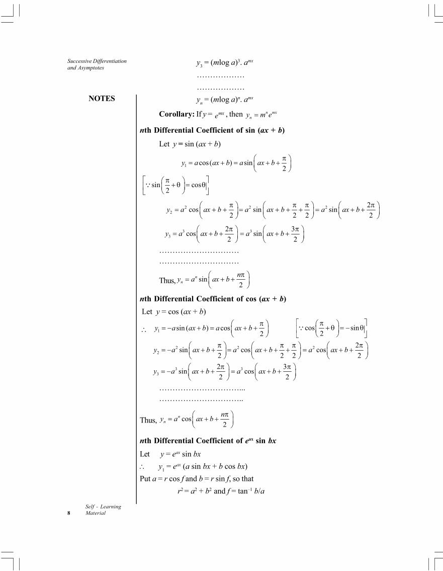
yn = (mlog a)n. amx
Corollary: If y = mxe , then n mxny m e
nth Differential Coefficient of sin (ax + b)
Let y = sin (ax + b)
1 cos( ) sin2
y a ax b a ax b
sin cos2
2 2
2 cos sin2 2 2
y a ax b a ax b
2 sin
2a ax b
3
3 cos2
y a ax b
3 sin
2a ax b
……………………………………………………
Thus, sin2
nn
ny a ax b
nth Differential Coefficient of cos (ax + b)
Let y = cos (ax + b)
1 sin ( ) cos2
y a ax b a ax b
cos sin
2
2 2
2 sin cos2 2 2
y a ax b a ax b
2 cos
2a ax b
3
3 sin2
y a ax b
3 cos
2a ax b
…………………………...…………………………..
Thus, cos2
nn
ny a ax b
nth Differential Coefficient of eax sin bx
Let y = eax sin bx
y1 = eax (a sin bx + b cos bx)
Put a = r cos f and b = r sin f, so that
r2 = a2 + b2 and f = tan–1 b/a
NOTES
Successive Differentiationand Asymptotes
Self - LearningMaterial 9
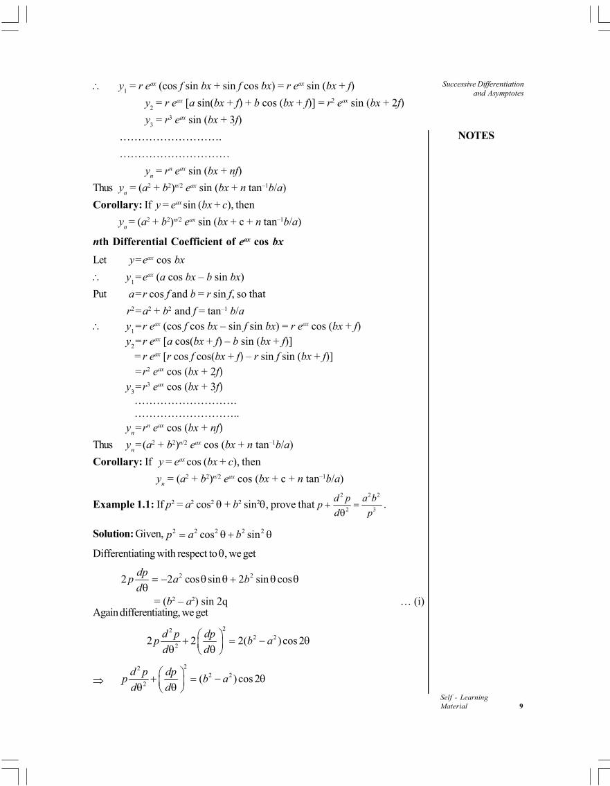
y1 = r eax (cos f sin bx + sin f cos bx) = r eax sin (bx + f)
y2 = r eax [a sin(bx + f) + b cos (bx + f)] = r2 eax sin (bx + 2f)
y3 = r3 eax sin (bx + 3f)
……………………….
…………………………
yn = rn eax sin (bx + nf)
Thus yn = (a2 + b2)n/2 eax sin (bx + n tan–1b/a)
Corollary: If y = eax sin (bx + c), then
yn = (a2 + b2)n/2 eax sin (bx + c + n tan–1b/a)
nth Differential Coefficient of eax cos bx
Let y=eax cos bx
y1=eax (a cos bx – b sin bx)
Put a=r cos f and b = r sin f, so that
r2=a2 + b2 and f = tan–1 b/a y
1=r eax (cos f cos bx – sin f sin bx) = r eax cos (bx + f)
y2=r eax [a cos(bx + f) – b sin (bx + f)]=r eax [r cos f cos(bx + f) – r sin f sin (bx + f)]=r2 eax cos (bx + 2f)
y3=r3 eax cos (bx + 3f)……………………….………………………..
yn=rn eax cos (bx + nf)
Thus yn=(a2 + b2)n/2 eax cos (bx + n tan–1b/a)
Corollary: If y = eax cos (bx + c), then
yn = (a2 + b2)n/2 eax cos (bx + c + n tan–1b/a)
Example 1.1: If p2 = a2 cos2 + b2 sin2, prove that2 2 2
2 3
d p a bp
d p
.
Solution: Given, 2 2 2 2 2cos sinp a b
Differentiating with respect to , we get
2 22 2 cos sin sin cosdp
p a bd
= (b2 – a2) sin 2q … (i)Again differentiating, we get
222 2
22 2 2( )cos 2
d p dpp b a
d d
22
2 22
( ) cos 2d p dp
p b ad d
Successive Differentiationand Asymptotes
NOTES
Self - Learning10 Material
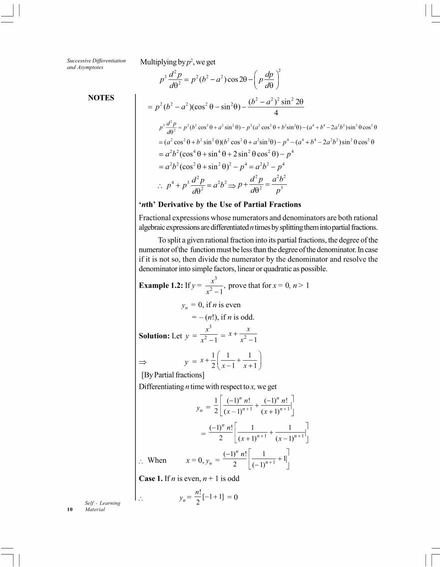
Multiplying by p2, we get22
3 2 2 22
( ) cos 2d p dp
p p b a pd d
2 2 2 2
2 2 2 2 ( ) sin 2( )(cos sin )
4
b ap b a
23 2 2 2 2 2 2 2 2 2 4 4 2 2 2
2( cos sin ) ( cos sin ) ( 2 )sin cos
d pp p b a p a b a b a b
d
2 2 2 2 2 2 2 4 4 4 2 2 2( cos sin )( cos sin ) ( 2 )sin cosa b b a p a b a b 2 2 4 4 2 4(cos sin sin cos )a b p 2 2 2 2 4(cos sina b p 2 2 4a b p
2
4 3 2 22
d pp p a b
d
2 2 2
2 3
d p a bp
d p
‘nth’ Derivative by the Use of Partial Fractions
Fractional expressions whose numerators and denominators are both rationalalgebraic expressions are differentiated n times by splitting them into partial fractions.
To split a given rational fraction into its partial fractions, the degree of thenumerator of the function must be less than the degree of the denominator. In caseif it is not so, then divide the numerator by the denominator and resolve thedenominator into simple factors, linear or quadratic as possible.
Example 1.2: If y = 3
2,
1
x
x prove that for x = 0, n > 1
ny = 0, if n is even
= – (n!), if n is odd.
Solution: Let y = 3
2 1
x
x = 2 1
xx
x
y = 1 1 1
2 1 1x
x x
[By Partial fractions]
Differentiating n time with respect to x, we get
ny = 1 1
1 ( 1) ! ( 1) !
2 ( – 1) ( 1)
n n
n n
n n
x x
= 1 1
( 1) ! 1 1
2 ( 1) ( 1)
n
n n
n
x x
When x = 0, ny = 1
( 1) ! 11
2 ( 1)
n
n
n
Case 1. If n is even, n + 1 is odd
ny = ![ 1 1]
2
n = 0
NOTES
Successive Differentiationand Asymptotes
Self - LearningMaterial 11
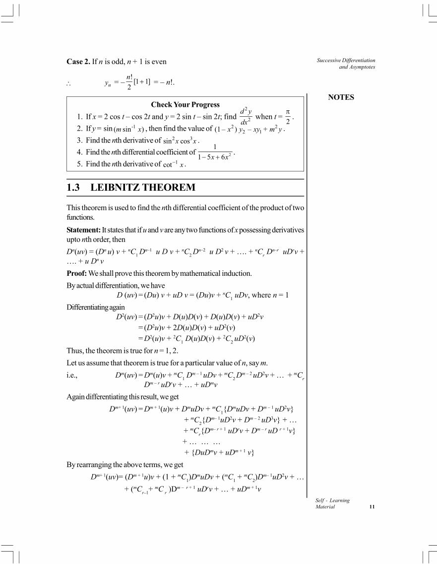
Case 2. If n is odd, n + 1 is even
ny = –![1 1]
2
n = – n!.
Check Your Progress
1. If x = 2 cos t – cos 2t and y = 2 sin t – sin 2t; find 2
2
d y
dx when t =
2
.
2. If y = sin -1( sin )m x , then find the value of 2 22 1(1 – ) –x y xy + m y .
3. Find the nth derivative of 2 3sin cosx x .
4. Find the nth differential coefficient of 2
1
1 5 6 x x.
5. Find the nth derivative of 1cot x .
1.3 LEIBNITZ THEOREM
This theorem is used to find the nth differential coefficient of the product of twofunctions.
Statement: It states that if u and v are any two functions of x possessing derivativesupto nth order, then
Dn(uv) = (Dn u) v + nC1 Dn–1 u D v + nC
2 Dn–2 u D2 v + …. + nC
r Dn–r uDrv +
…. + u Dn v
Proof: We shall prove this theorem by mathematical induction.
By actual differentiation, we haveD (uv) = (Du) v + uD v = (Du)v + nC
1 uDv, where n = 1
Differentiating againD2(uv) = (D2u)v + D(u)D(v) + D(u)D(v) + uD2v
= (D2u)v + 2D(u)D(v) + uD2(v)= D2(u)v + 2C
1 D(u)D(v) + 2C
2 uD2(v)
Thus, the theorem is true for n = 1, 2.
Let us assume that theorem is true for a particular value of n, say m.
i.e., Dm(uv) = Dm(u)v + mC1 Dm – 1 uDv + mC
2 Dm – 2 uD2v + … + mC
r
Dm – r uDrv + … + uDmv
Again differentiating this result, we get
Dm+ 1(uv) = Dm + 1(u)v + DmuDv + mC1{DmuDv + Dm – 1 uD2v}
+ mC2{Dm– 1uD2v + Dm – 2 uD3v} + …
+ mCr{Dm– r + 1 uDrv + Dm – r uD r + 1v}
+ … … … + {DuDmv + uDm + 1 v}
By rearranging the above terms, we get
Dm+ 1(uv)= (Dm + 1u)v + (1 + mC1)DmuDv + (mC
1 + mC
2)Dm– 1uD2v + …
+ (mCr–1
+ mC r )Dm – r + 1 uDrv + … + uDm + 1v
Successive Differentiationand Asymptotes
NOTES
Self - Learning12 Material
As we know that mCr–1
+ mC r = m + 1C
r
Putting r = 1, mC0 + mC
1 = m + 1C
1;
Putting r = 2, mC1 + mC
2 = m + 1C
2 etc.
1 1 1 1 1 2 1 1 11 2( ) ( ) ..... ..... .m m m m m m m m r r mD uv D u v C D uDv C D uD v C D uD v u D v
1 1 1 1 1 2 1 1 1( ) ( ) ..... ..... .m m m m m m m m r r mrD uv D u v C D uDv C D uD v C D uD v u D v
This shows that if the theorem is true for n = m, it is also true for n = m + 1.
But the theorem is true for n = 1; therefore by the principle of mathematicalinduction, the theorem is true for every positive integral value of n.
Note: In applying this theorem we take u as that function whose nth derivative isknown and v as that function which is of the form xn.
Example 1.3: If y = a cos (log x) + b sin (log x), then show that
(a) 22 1x y xy y = 0
(b) 2 22 1(2 1) ( 1)n n nx y n xy n y = 0
Solution: We have y = a cos (log x) + b sin (log x)
1y =1 1
sin (log ) cos (log ) .a x b xx x
1xy = sin (log ) cos (log )a x b x
Differentiating again, we have
2 1xy y =1 1
cos(log ) . sin (log ) .a x b xx x
22 1x y xy = cos (log ) sin (log )a x b x = – y
22 1x y xy y =0 …(i)
This proves the first part.Again differentiating Equation (i) n times by Leibnitz’s Theorem, we have
22 1 1
( 1)2 . 2 .
2!n n n n n nn n
x y ny x y y x n y y
= 0
2 22 1(2 1) ( 1)n n nx y n xy n y = 0
Example 1.4: If y = 2 2[log { (1 )}]x x , prove that
2 22 1(1 ) (2 1)n n nx y n xy n y = 0.
NOTES
Successive Differentiationand Asymptotes
Self - LearningMaterial 13
Solution: Given, y = 2 2[log { (1 )}]x x ,
y1= 2
2 2
1 22 log (1 ) . . 1
(1 ) 2 (1 )
xx x
x x x
= 22
2 2
1 12 log (1 ) . .
(1 ) 1
x xx x
x x x
1y = 2
2
12 log { (1 )}.
(1 )x x
x
Cross-multiplying and squaring both sides, we get
2
2 2 21(1 ) 4 log( 1 4x y x x y
Differentiating both the sides with respect to x, we get2 2
1 2 1(1 ) . 2 2x y y xy = 14y
22 1(1 )x y xy = 2 [Dividing by 2y
1]
Differentiating n times by Leibnitz’s theorem, we get
22 1 1(1 ) 2 ( 1)n n n n nx y nxy n n y xy ny = 0
2 22 1(1 ) (2 1)n n nx y n xy n y = 0
Calculation of ‘nth’ Derivative at x = 0
Sometimes it is difficult to calculate the nth derivative of a function in general. Inthat case its value can be calculated at x = 0 by the application of Leibnitz’sTheorem.
Working Rule:
(i) Let the given function be y.
(ii) Find dy
dx and then, take L.C.M, if possible.
(iii) If square roots are present, square both sides and then try to get y in R.H.S.
(iv) Find the equation in y2, y
1, y by differentiating both sides of the equation
obtained in Step (iii).
(v) Differentiate the equation so obtained n times, by Leibnitz’s Theorem.
(vi) Put x = 0 in equation obtained in all the steps above from Step (i) toStep (v).
(vii) Put n = 1, 2, 3, 4 in the last equation of Step (vi).
(viii) Discuss the cases when n is even or odd.
Successive Differentiationand Asymptotes
NOTES
Self - Learning14 Material
Example 1.5: If y = 2[ (1 )]mx x , find 0( )ny .
Solution: We have y= 2[ (1 )]mx x …(i)
1y = 2 1
2
2[ (1 )] 1
2 (1 )
m xm x x
x
= 2
2[ (1 )]
(1 )
mmx x
x
1y =2(1 )
my
x…(ii)
2 21(1 )x y = 2 2m y
Differentiating again, we have
2 21 2 1(1 ) 2 2x y y xy = 2
12m yy
i.e., 22 1(1 )x y xy = 2m y
… (iii)
Differentiating Equation (iii) n times by Leibnitz’s Theorem, we have
22 1 1
( 1)(1 ) (2 ) 2
1.2n n n n nn n
x y ny x y xy ny
= 2nm y
2 2 22 1(1 ) (2 1) ( )n n nx y n xy n m y = 0 …(iv)
Putting x = 0 in Equations (i), (ii), (iii) and (iv), we get
0( )y = 1, 1 0( )y = m, 2 0( )y = 2m ,
2 0( )ny = 2 20( ) ( )nm n y . …(v)
Case 1: When n is odd. Putting n = 1, 3, 5,… in Equation (v), we have
1 0( )y = m.
3 0( )y = 2 21 0( 1 ) ( )m y = 2 2( 1 )m m ,
5 0( )y = 2 23( 3 ) ( )m y
= 2 2 2 2( 3 ) ( 1 ) ,m m m … … ….
0( )ny = 2 2[ ( 2) ]m n … 2 2 2 2( 3 ) ( 1 ) .m m m
Case 2: When n is even. Putting n = 2, 4, 6,… in Equation (v), we have
2 0( )y = 2m .
4 0( )y = 2 22 0( 2 ) ( )m y = 2 2 2( 2 )m m ,
6 0( )y = 2 24 0( 4 ) ( )m y
= 2 2 2 2 2( 4 ) ( 2 ) ,m m m … … ….
0( )ny = 2 2[ ( 2) ]m n … 2 2 2 2 2( 4 ) ( 2 )m m m
NOTES
Successive Differentiationand Asymptotes
Self - LearningMaterial 15
Example 1.6: If y = 1 2(sin )- x , prove that
(a) 22 1(1 ) 2x y xy = 0
(b) 2 22 1(1 ) (2 1)n n nx y n xy n y = 0
Deduce that 2
0lim
n
x n
y
y
= 2n and find (0)ny .
Solution: Given, y = 1 2(sin )x
1y = 1
2
12 (sin ) .
1x
x
… (i)
211 x y = 12sin x
Squaring both sides, we have
2 21(1 )x y = 1 24 (sin )x = 4y
Differentiating both sides with respect to x, we have2 2
1 2 1(1 ) 2 2x y y xy = 14y
22 1(1 ) 2x y xy = 0 [Dividing both sides by 12y ] …(ii)
Which proves (a).
Differentiating 22 1(1 ) 2x y xy = 0 n-times by Leibnitz’s Theorem, we get
22 1 1
( 1)(1 ) ( 2 ) ( 2) [ .1]
2!n n n n nn n
y x ny x y y x ny
= 0 …(iii)
2 22 1(1 ) (2 1)n n nx y n xy n y = 0
2 1 2(2 1)
1n n
xy n y
x
= 2
21nn y
x
When x 0,2
0lim n
x n
y
y
= 2
20lim
1x
n
x = 2n
From Equation (i), when x = 0, 1 (0)y = 0
From Equation (ii), when x = 0, 2 (0)y = 2
From Equation (iii), when x = 0, 2 (0)ny = 2nn y (0)
From Equation (iv), when n = 1, 3 (0)y = 211 (0)y = 0
n = 2, 4 (0)y = 222 (0)y = 22 . 2
n = 3, 5 (0)y = 233 (0)y = 0
n = 4, 6 (0)y = 244 (0)y = 2 24 . 2 . 2
If n is odd, ny (0) = 0
and if n is even, ny (0) = 2 2 2 22 . 2 . 4 . 6 ... ( 2)n .
Successive Differentiationand Asymptotes
NOTES
Self - Learning16 Material
Check Your Progress
6. Find the nth derivative of 3 axx e .
7. If y = 2 sinx x , then find the value of yn.
8. If y = 1sin ,x find ( )n xy = 0.
9. If u = tan-1x, prove that (1 + x)2u2 + 2xu
1 = 0,
22 1(1 ) 2( 1) ( 1) 0n n nx u n xu n n u
and hence determine the values of all the derivatives of n with respect to x,when x = 0.
1.4 MACLAURIN AND TAYLOR SERIESEXPANSIONS
A set of terms which are connected by positive or negative signs and are arrangedaccording to some fixed definite law are called a series. There are two types ofseries, finite series and infinite series according to the number of terms (finite orinfinite) it contains.
For example, 1 + 4 + 7 + 10 + 13 is a finite series containing five terms
whereas 1 1 1
1 ...2 4 6
is an infinite series.
If nS = 1 2 3 ... na a a a , then (S )n is called the sequence of partialsums of the series. If { }na is a sequence, then 1 2 3 ... ....na a a a is called
an infinite series which is written as 1
nn
a
.
1.4.1 Taylor’s Infinite Series
Theorem 1.1: Let f(x) be a function such that:
(a) It has continuous derivatives of all order in the open interval (a, a + h) and
(b) Taylor’s remainder, Rn = ( )
!
nnh
f a hn
, 0 < < 1 tends to 0 as n
then f (a + h) = 2
( ) ( ) ( ) ... ( ) ...2! !
nnh h
f a hf a f a f an
…(1)
Proof: Let f(x) be a function, which possesses continuous derivates of all order inthe open interval (a, a + h). Then, for every integer n, however large, there is acorresponding Taylor’s development with Lagrange’s form of remainder, i.e.,
f (a + h)=2 1
1( ) ( ) ( ) ... ( ) R2! ( 1)!
nn
nh h
f a hf a f a f an
,
NOTES
Successive Differentiationand Asymptotes
Self - LearningMaterial 17
where Rn = ( ),!
nnh
f a hn
0 < < 1
We can write the above expression as f (a + h) = S Rn n ,
whereSn = 2 1
1( ) ( ) ( ) ... ( )2! ( 1)!
nnh h
f a hf a f a f an
.
Suppose, Rn tends to 0 as n . Then, we have
lim Snn =
2
( ) ( ) ( ) ...2!
hf a hf a f a
And hence f (a + h) = 2
( ) ( ) ( ) ...2!
hf a hf a f a
Hence proved.
This theorem expands f (a + h) to an infinite series of ascending integral powers ofh and the infinite series thus obtained is called Taylor’s infinite series.
Expressing Taylor’s Infinite Series in Different Forms
(1) On putting a = x in Equation (1), we get
f (x + h) = 2
( ) ( ) ( ) ... ( ) ...2! !
nnh h
f x hf x f x f xn
(2) On putting a + h = b or h = b – a in Equation (1), we getf(b)
=2( ) ( )
( ) ( ) ( ) ( ) ... ( ) ...2! !
nnb a b a
f a b a f a f a f an
(3) On putting a + h = x or h = x – a, we get
f(x) =2( ) ( )
( ) ( ) ( ) ( ) ... ( ) ...2! !
nnx a x a
f a x a f a f a f an
Here, we get the expansion of f(x) to an infinite series of ascending integral powersof (x – a).
1.4.2 Maclaurin’s Infinite Series
Let f(x) be a function such that
(a) It has continuous derivatives of all orders in the open interval (0, x), and
(b) Maclaurin’s remainder Rn = ( )!
nnx
f xn
0 as n
then f (x) = 2
(0) (0) (0) .... (0) ...2! !
nnx x
f xf f fn
.
Successive Differentiationand Asymptotes
NOTES
Self - Learning18 Material
This is called Maclaurin’s infinite series.
We can obtain the above expression by putting a = 0, and h = x in Taylor’s infiniteseries.
Note: Let the function f (x) be denoted by y, then the above expansion can bewritten as:
y = 2
1 2(0) . (0) (0) ... (0) ...2! !
n
nx x
y x y y yn
where 1 2(0), (0), (0) ,..., (0)ny y y y are the values of 1 2, , ,..., ny y y y respectivelyat x = 0.
Example 1.7: Expand sin ( 1)xe upto and including the term of 4x .
Solution: We know that xe = 2 3 4
1 ...2! 3! 4!
x x xx
1xe =2 3 4
...2! 3! 4!
x x xx = t (say)
sin ( 1)xe = sin t = 3 5
...3! 5!
t tt
=
32 3 4 2 3 41... ... ...
2 6 24 6 2 6 24
x x x x x xx x
=2 3 4 2 3
3 21... 3 ... ...
2 6 24 6 2 6
x x x x xx x x
= 2 41 5...
2 24x x x
Example 1.8: Expand sin x and cos x in powers of x and hence find cos 18º uptofour decimal places.
Solution: (a) Let f(x) = sin x f(0) = 0
Now ( )f x = cos x (0)f = 1
( )f x = – sinx (0)f = 0
( )f x = cos x (0)f = –1
( )ivf x = sin x (0)ivf = 0
( )vf x = cos x (0)vf = 1
………………….
By Maclaurin’s expansion, we have
f (x) = 2 3
(0) (0) (0) (0) ...2! 3!
x xf xf f f
NOTES
Successive Differentiationand Asymptotes
Self - LearningMaterial 19
sin x = 2 3 4 5
0 .1 .0 ( 1) .0 .1 ...2! 3! 4! 5!
x x x xx
= 3 5
...3! 5!
x xx
(b) Let f(x) = cos x f(0) = 1
Now ( )f x = – sin x (0)f = 0
( )f x = – cos x (0)f = –1
( )f x = sin x (0)f = 0
( )ivf x = cos x (0)ivf = 1
( )vf x = – sin x (0)vf = 0
( )vif x = – cos x (0)vif = –1
cos x = 2 3 4 5 6
1 . 0 ( 1) . 0 .1 . 0 . ( 1) ...2! 3! 4! 5! 6!
x x x x xx
= 2 4 6
1 ...2! 4! 6!
x x x
Let x = 18º = 10
= 0.314
cos 18º = 2 4 6
1 1 11 ...
2! 10 4! 10 6! 10
= 2 4 61 1 11 (0.314) (0.314) (0.314) ...
2! 4! 6!
= 1 – .04929 + .00040 + … = .9511 (upto four decimal places)
1.4.3 Application of Taylor’s Infinite Series to Expandf(x + h)
1. Let f (x + h) be the given function.
2. Obtain f(x) by putting h = 0.
3. Differentiate f(x) a number of times and obtain ( ), ( ), ( ), ...f x f x f x , etc.
4. Substitute the values of ( ), ( ), ( ), ...f x f x f x in
f (x + h) = 2 3
( ) ( ) ( ) ( ) ...2! 3!
h hf x hf x f x f x
Example 1.9: If f(x) = 3 22 5 11,x x x find the value of 9
10f
with the help
of Taylor’s series for f(x + h).
Successive Differentiationand Asymptotes
NOTES
Self - Learning20 Material
Solution: f (x) = 3 22 5 11x x x
Now by Taylor’s Theorem, we have
f(x + h) = 2 3
( ) ( ) ( ) ( ) ...2! 3!
h hf x hf x f x f x ...(i)
Putting x = 1 and h = 1
10 in Equation (i), we get
11
10f
= 2 3
1 1 1 1 1(1) (1) (1) (1) ...
10 2! 10 3! 10f f f f
…(ii)
Here, f(x) = 3 22 5 11x x x f(1) = 9
Now, ( )f x = 23 4 5x x (1)f = 2
( )f x = 6x + 4 (1)f = 10
( )f x = 6 (1)f = 6
Putting these values in Equation (ii), we have
9
10f
= 1 1 1
9 (2) (10) (6)10 200 6000
= 9 0.2 0.05 0.001 = 8.849
Example 1.10: Expand log sin x in powers of (x – 2).
Solution: Let f(x) = log sin x
log sin x = f(x) = f(2 + (x – 2)]
= f(2 + h) (where, h = x – 2)
By Taylor’s Theorem for x = 2, we have
f(2 + h) = 2 3
(2) '(2) ''(2) '''(2) ...2
h hf hf f f
… (i)
Now, f(x) = log sin x f(2) = log sin 2
f ‘(x) = cos
cotsin
xx
x , f (2) = cot 2
f (x) = – cosec2 x, f (2) = – cosec2 2 f (x) = – 2cosec x(– cosec x cot x) = 2 cosec2 x cot x f(2) = 2cosec2 2 cot 2 …………………
From Equation (i), we have
2 3
2 2( 2) ( 2)logsin logsin 2 ( 2)cot 2 cosec 2 2cosec 2cot 2 ...
2 3
x xx x
NOTES
Successive Differentiationand Asymptotes
Self - LearningMaterial 21
Solutions Using Differential Equations
Example 1.11: Show that1
2 2 2 2 2 2 2 2 2sin 3 4 5( 1) ( 2 ) ( 1)( 3 )
1 ...2
a x a x a a a a a a ae ax x x x
and hence deduce that 2 31 sin sin sine
Solution: Let y = 1sina xe … (i)
1sin
1 2 2
.
1 1
a xe a ayy
x x
… (ii)
By squaring and cross multiplying,
(1 – x2)y12 = a2y2
Differentiating again, we get
(1 – x2)2y1y
2 – 2xy
12= a2 2yy
1 (1 – x2)y
2 – xy
1 – a2 y = 0 … (iii)
Differentiating the Equation (iii), n times by Leibnitz’s Theorem, we have
yn+2
(1 – x2) + nC1y
n + 1(–2x) + nC
2y
n (–2) –[y
n + 1x + nC
1y
n.1]= a2y
n
(1 – x2)yn+2
– (2n + 1)xyn+1
– (n2 + a2)yn = 0
Putting x = 0, we have yn+2
(0) = (n2 + a2)yn(0) … (iv)
From Equations (i), (ii) and (iii), we have
y(0) = 1, y1(0) = a, y
2(0) = a2,
Now, putting n = 1, 2, 3, …, in Equation (iv), we get
y3(0) = a(a2 +12),
y4(0) = a2(a2 + 22),
y5(0) = a(a2 +12) (a2 +32) …………………………..
Thus, by Maclaurin’s Theorem,
2 3 4 5
1 2 3 4 5(0) (0) (0) (0) (0) (0) ....2
x x x xy y xy y y y y
1
2 2 2 2 2 2 2 2 2 2 2sin 3 4 5( 1 ) ( 2 ) ( 1 )( 3 )
1 ...2
a x a x a a a a a a ae ax x x x
2 2 2 2 2 2 2 2 2 2 2
sin 3 4 5( 1 ) ( 2 ) ( 1 )( 3 )1 ...
a x a a a a a a ae ax x x x
To get the second part, let a = 1 and x = sin q,
2 3 41 2 51 sin sin sin sin ...
2e
Solutions Using Differentiation and Integration Method
Example 1.12: Expand 2log 1x + x =
3 51 1.3. . ...
2 3 2.4 5
x xx
Successive Differentiationand Asymptotes
NOTES
Self - Learning22 Material
Solution: Let y = 2log[ + (1+ )].x x
y1 = 2 2
1 21
1 2 1
x
x x x
= 2
1
1 x = (1 +x2)–1/2
Expanding by binomial theorem, we get
2 41
1 1.31 ...
2 2.4y x x
Integrating both sides w.r.t x within the limits 0 to x, we get
y = 3 51 1.3
. . ...2 3 2.4 5
x xx
2log 1x + x = 3 51 1.3
. . ...2 3 2.4 5
x xx
Check Your Progress
10. Expand tan x in power of 4
x
upto first four terms.
1.5 ASYMPTOTES
A straight line at a finite distance from the origin, is said to be an asymptote to aninfinite branch of a curve, if the perpendicular distance of any point P on thatbranch from the straight line tends to be zero as P tends to infinity along the branchof the curve.
We can also define asymptotes as a straight line which is at a finite distancefrom the origin and cuts a curve in two points at an infinite distance from the origin.
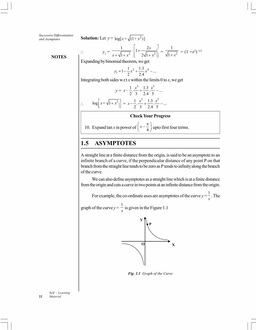
For example, the co-ordinate axes are asymptotes of the curve y =1
x. The
graph of the curve y = 1
x is given in the Figure 1.1
Y
O X
P
Fig. 1.1 Graph of the Curve
NOTES
Successive Differentiationand Asymptotes
Self - LearningMaterial 23
Asymptotes are usually classified as the following:
Vertical Asymptotes
Horizontal Asymptotes
Oblique Asymptotes
Vertical and Horizontal Asymptotes
Vertical Asymptotes: The asymptotes parallel to y-axis are called verticalasymptotes.
A line x = a is a vertical asymptote of a curve if either
lim ( )x a
f x
or lim ( )x a
f x
.
Horizontal Asymptotes: The asymptotes parallel to x-axis are calledhorizontal asymptotes.
A line y = b is a horizontal asymptote of a curve y = f(x) if either
lim ( )x
f x = b or lim ( )
x
f x b .
1.5.1 Asymptotes Parallel to Axes of Co-Ordinates
An asymptote of a curve is a line such that the distance between the curve and theline approaches zero as they tend to infinity.
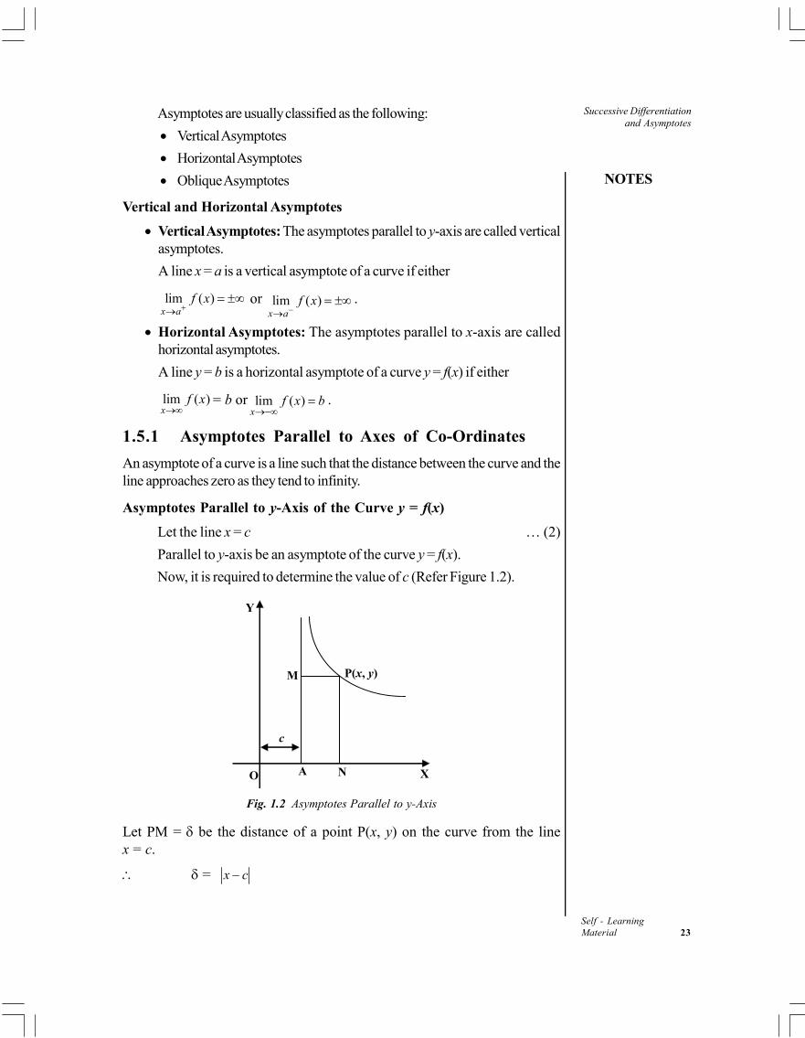
Asymptotes Parallel to y-Axis of the Curve y = f(x)
Let the line x = c … (2)
Parallel to y-axis be an asymptote of the curve y = f(x).
Now, it is required to determine the value of c (Refer Figure 1.2).
Y
O X
M
N A
c
P(x, y)
Figure 3.2 Fig. 1.2 Asymptotes Parallel to y-Axis
Let PM = be the distance of a point P(x, y) on the curve from the linex = c.
= x c
Successive Differentiationand Asymptotes
NOTES
Self - Learning24 Material
(Perpendicular distance of a point (x1, y
1) from the line,
ax + by + c = 0 is 1 1
2 2
ax by c
a b
)
Then, by the definition of an asymptote, if line Equation (2) is an asymptote of thecurve, then 0 as P .
As
P , = x c 0 or x c.
P(x, y) is tend to infinity, y co-ordinate must tend to (+ or )
limy
x c
, i.e., x c as y … (3)
Thus, to find the asymptotes parallel to y-axis, we find from the given equation,the definite values c
1, c
2, … to which x tends, as y + or . Then
x = c1, x = c
2,… are the asymptotes of the curve parallel to y-axis.
Corollary: Similarly, to find asymptotes parallel to x-axis, we find the definitevalues d
1, d
2, … from the equation of the curve to which y tends as x + or
. Then, the asymptotes parallel to x-axis are y = d1, y = d
2, and so on.
Asymptotes Parallel to the Axes for an Algebraic Curve
Asymptotes Parallel to the y-Axis
Let the equation of the curve be,
1 2 2 1 1 2 2 1
0 1 2 1 1 2 1
2 3 3 22 3 1
( ... ) ( ... )
( ... ) 0
n n n n n n n n nn n n n
n n n nn n
a y a y x a y x a yx a x b y b y x b yx b x
c y c y x c yx c x
X O
Y
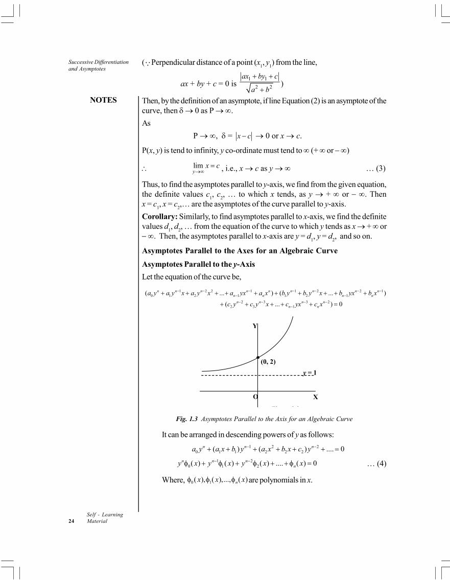
(0, 2)
y = 1
Figure 3.3
Fig. 1.3 Asymptotes Parallel to the Axis for an Algebraic Curve
It can be arranged in descending powers of y as follows:
1 2 20 1 1 2 2 2( ) ( ) .... 0n n na y a x b y a x b x c y
1 20 2) ) ) .... ) 0
n n nny x y x y x x … (4)
Where, 1), ),..., ) nx x x are polynomials in x.
NOTES
Successive Differentiationand Asymptotes
Self - LearningMaterial 25
Dividing Equation (4) by ny , we have
0 22) ) ) .... ) 0
nn
x x x xy y y ...(5)
Let x = c be an asymptote of Equation (4) parallel to y-axis, then lim
y
x c .
Therefore, Equation (3) gives 0(c) = 0, so that c is a root of the equation
0(x) = 0.
Working Rule: Asymptotes parallel to the axis of y can be obtained byequating to zero the coefficient of the highest degree term of y in the equation ofthe curve.
If the coefficient of the highest powers of y is a constant or if its linearfactors are all imaginary, there will be no asymptote parallel to y-axis.
Asymptotes Parallel to the x-Axis
Working Rule: Asymptotes parallel to the axis of x can be obtained by equatingto zero the coefficient of the highest degree term of x in the equation of the curve.
If the coefficient of the highest powers of x is a constant or if its linearfactors are all imaginary, there will be no asymptote parallel to x-axis.
Example 1.13: Find all the asymptotes, parallel to the axes of the given curve2 2
2 21
a b
x y .
Solution: The given curve is 2 2
2 21
a b
x y
2 2 2 2 2 2 0x y b x a y … (i)
As Equation (i) is of fourth degree, it cannot have more than four asymptotes.
In order to find out the asymptotes parallel to x -axis, equating the coefficientof highest power of x, i.e., x2 in (i) to zero
2 2y b = 0 y = ± bi
Which gives the imaginary asymptotes.
Again equating to zero, the coefficient of highest power of y, i.e., y2 in (i),the asymptotes parallel to the y-axis are given by x2 – a2 = 0, x = + a whichgives two real asymptotes parallel to y-axis.
Hence, the only asymptotes are x = + a.
1.5.2 Oblique Asymptotes
An asymptote which is neither parallel to x-axis nor parallel to y-axis is called anoblique asymptote of the curve (Refer Figure 1.4).
Successive Differentiationand Asymptotes
NOTES
Self - Learning26 Material
Y
O X
M P(x, y)
Figure 3.4
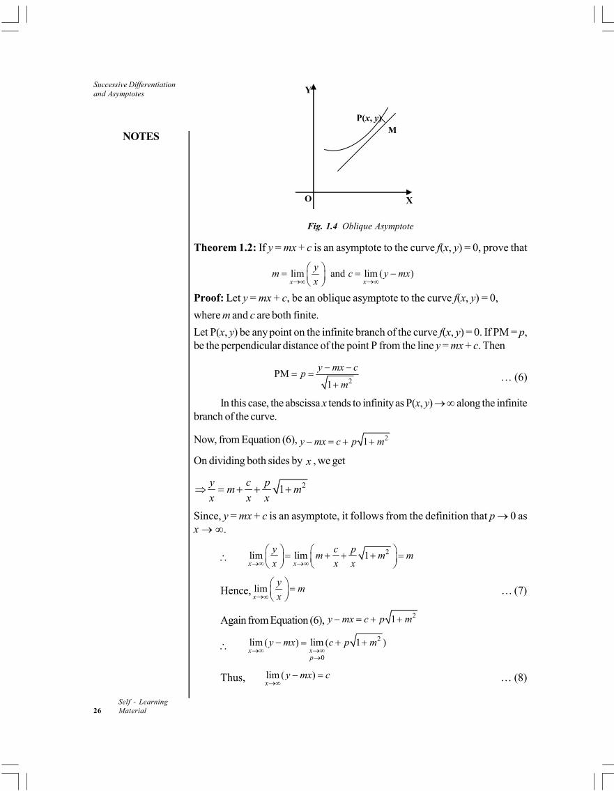
Fig. 1.4 Oblique Asymptote
Theorem 1.2: If y = mx + c is an asymptote to the curve f(x, y) = 0, prove that
lim and lim ( )x x
ym c y mx
x
Proof: Let y = mx + c, be an oblique asymptote to the curve f(x, y) = 0,
where m and c are both finite.
Let P(x, y) be any point on the infinite branch of the curve f(x, y) = 0. If PM = p,be the perpendicular distance of the point P from the line y = mx + c. Then
2PM
1
y mx cp
m
… (6)
In this case, the abscissa x tends to infinity as P(x, y) along the infinitebranch of the curve.
Now, from Equation (6), 21y mx c p m
On dividing both sides by x , we get
21y c p
m mx x x
Since, y = mx + c is an asymptote, it follows from the definition that p 0 asx .
2lim lim 1x x
y c pm m m
x x x
Hence, limx
ym
x
… (7)
Again from Equation (6), 21y mx c p m
2
0
lim ( ) lim ( 1 )x x
p
y mx c p m
Thus, lim ( )x
y mx c
… (8)
NOTES
Successive Differentiationand Asymptotes
Self - LearningMaterial 27
Thus, if y = mx + c is an oblique asymptote to any curve f(x, y) = 0, then
lim and lim ( )x x
ym c y mx
x
.
Oblique Asymptotes of the General Algebraic Curves
Let the general algebraic equation of the curve of nth degree be
1 2 2 1 2 3 2 10 1 2 1 2 3
2 3 4 2 21 2 3
( ... ) ( ... )
( ... ) ... ( ) 0
n n n n n n n nn n
n n n nn
a y a y x a y x a x b y b y x b y x b x
c y c y x c y x c x ax by c
The above equation can be put into the form
1 21 2 0... 0n n n
n n n
y y y yx x x
x x x x
… (9)
where n
y
x
represents an expression of nth degree in y
x.
Let y = mx + c … (10)
be an asymptote of the curve, where m and c are finite,
where, lim and lim ( )x x
ym c y mx
x
Dividing both sides of Equation (9) by xn, we get
1 2 02
1 1 1.... 0n n n n
y y y y
x x x x x x x
Taking limit x , limx
ym
x
on both sides, we get
( ) 0n m … (11)
which is in general an nth degree polynomial equation in m. The real values of mobtained from Equation (11) give slopes of the asymptotes. If m = 0 is a root ofEquation (11), then it corresponds to an asymptote parallel to x-axis.
Let y mx = p, so that p c as x . lim ( )x
y mx c
Now, y = mx + p
Dividing both sides by x ,we get y p
mx x
On substituting the value of y
x in Equation (9), we get
1 21 2 .... 0n n n
n n n
p p px m x m x m
x x x
… (12)
Successive Differentiationand Asymptotes
NOTES
Self - Learning28 Material
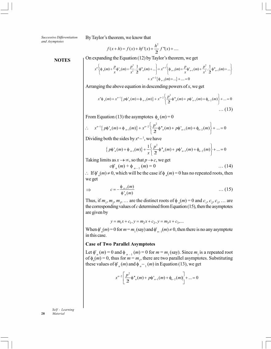
By Taylor’s theorem, we know that2
( ) ( ) '( ) ''( ) ....2
hf x h f x hf x f x
On expanding the Equation (12) by Taylor’s theorem, we get
2 21
1 1 12 2
22
1 1( ) ' ( ) . '' ( ) ... ( ) ' ( ) . '' ( ) ...
2 2
( ) ... .... 0
n nn n n n n n
nn
p p p px m m m x m m m
x x x x
x m
Arranging the above equation in descending powers of x, we get
2
1 21 1 2( ) ' ( ) ( ) '' ( ) ' ( ) ( ) ... 0
2n n n
n n n n n n
px m x p m m x m p m m
… (13)
From Equation (13) the asymptotes n (m) = 0
2
1 21 1 2' ( ) ( ) '' ( ) ' ( ) ( ) ... 0
2n n
n n n n n
px p m m x m p m m
Dividing both the sides by xn 1, we have
2
1 1 2
1' ( ) ( ) '' ( ) ' ( ) ( ) ... 0
2n n n n n
pp m m m p m m
x
Taking limits as x , so that p c, we getc
n (m) +
n – 1 (m) = 0 … (14)
If n(m) 0, which will be the case if
n(m) = 0 has no repeated roots, then
we get
1( )
' ( )n
n
mc
m
… (15)
Thus, if m1, m
2, m
3, … are the distinct roots of
n(m) = 0 and c
1, c
2, c
3, … are
the corresponding values of c determined from Equation (15), then the asymptotesare given by
1 1 2 2 3 3, , ,...y m x c y m x c y m x c
When n(m) = 0 for m = m
1 (say) and
n - 1(m) 0, then there is no any asymptote
in this case.
Case of Two Parallel Asymptotes
Let n (m) = 0 and
n – 1
(m) = 0 for m = m1 (say). Since m
1 is a repeated root
of n(m) = 0, thus for m = m
1, there are two parallel asymptotes. Substituting
these values of n (m) and
n
1 (m) in Equation (13), we get
22
1 2'' ( ) ' ( ) ( ) ... 02
nn n n
px m p m m
NOTES
Successive Differentiationand Asymptotes
Self - LearningMaterial 29
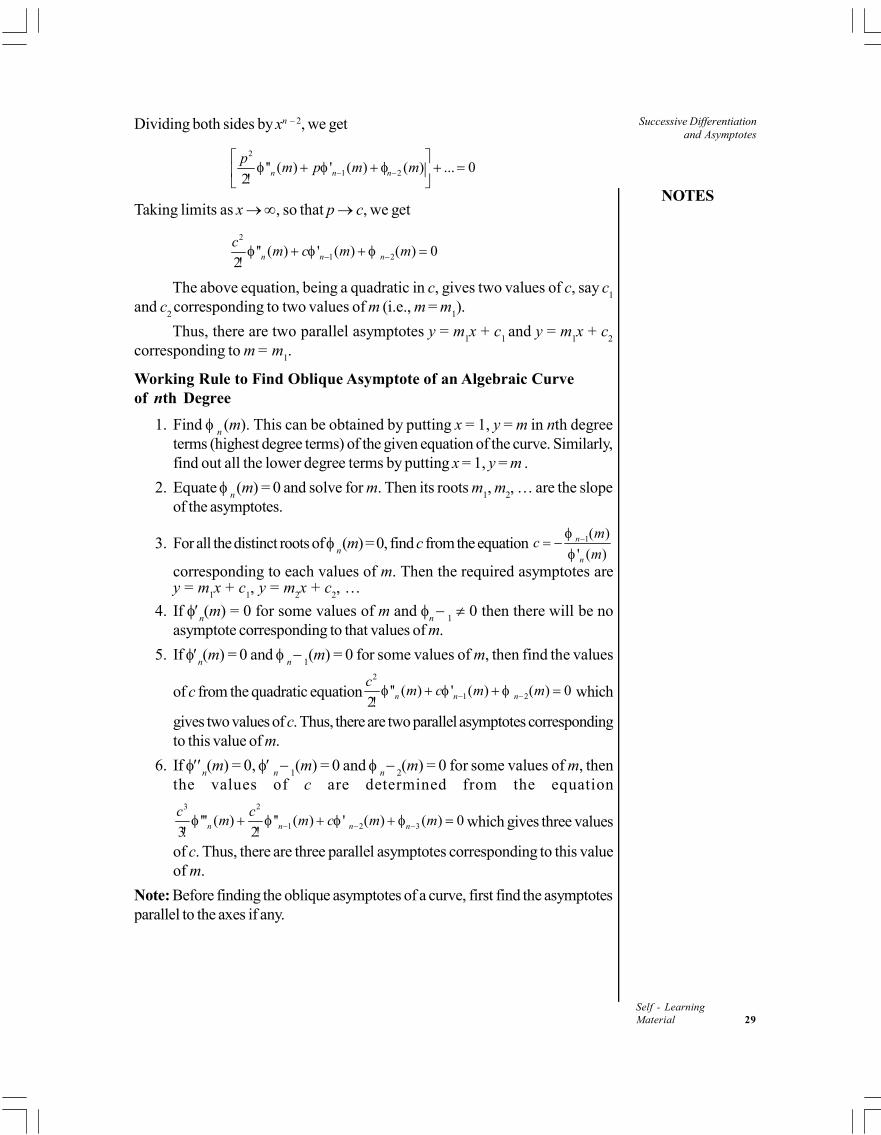
Dividing both sides by xn – 2, we get
2
1 2'' ( ) ' ( ) ( ) ... 02 n n n
pm p m m
Taking limits as x , so that p c, we get
2
1 2'' ( ) ' ( ) ( ) 02 n n n
cm c m m
The above equation, being a quadratic in c, gives two values of c, say c1
and c2 corresponding to two values of m (i.e., m = m
1).
Thus, there are two parallel asymptotes y = m1x + c
1 and y = m
1x + c
2
corresponding to m = m1.
Working Rule to Find Oblique Asymptote of an Algebraic Curveof nth Degree
1. Find n (m). This can be obtained by putting x = 1, y = m in nth degree
terms (highest degree terms) of the given equation of the curve. Similarly,find out all the lower degree terms by putting x = 1, y = m .
2. Equate n (m) = 0 and solve for m. Then its roots m
1, m
2, … are the slope
of the asymptotes.
3. For all the distinct roots of n (m) = 0, find c from the equation 1( )
' ( )n
n
mc
m
corresponding to each values of m. Then the required asymptotes arey = m
1x + c
1, y = m
2x + c
2, …
4. If n(m) = 0 for some values of m and
n
1 0 then there will be no
asymptote corresponding to that values of m.
5. If n(m) = 0 and
n
1(m) = 0 for some values of m, then find the values
of c from the quadratic equation2
1 2'' ( ) ' ( ) ( ) 02 n n n
cm c m m
which
gives two values of c. Thus, there are two parallel asymptotes correspondingto this value of m.
6. If n(m) = 0,
n
1(m) = 0 and
n
2(m) = 0 for some values of m, then
the values of c are determined from the equation3 2
1 2 3''' ( ) '' ( ) ' ( ) ( ) 03 2n n n n
c cm m c m m
which gives three values
of c. Thus, there are three parallel asymptotes corresponding to this valueof m.
Note: Before finding the oblique asymptotes of a curve, first find the asymptotesparallel to the axes if any.
Successive Differentiationand Asymptotes
NOTES
Self - Learning30 Material
1.5.3 Total Number of Asymptotes of a Curve
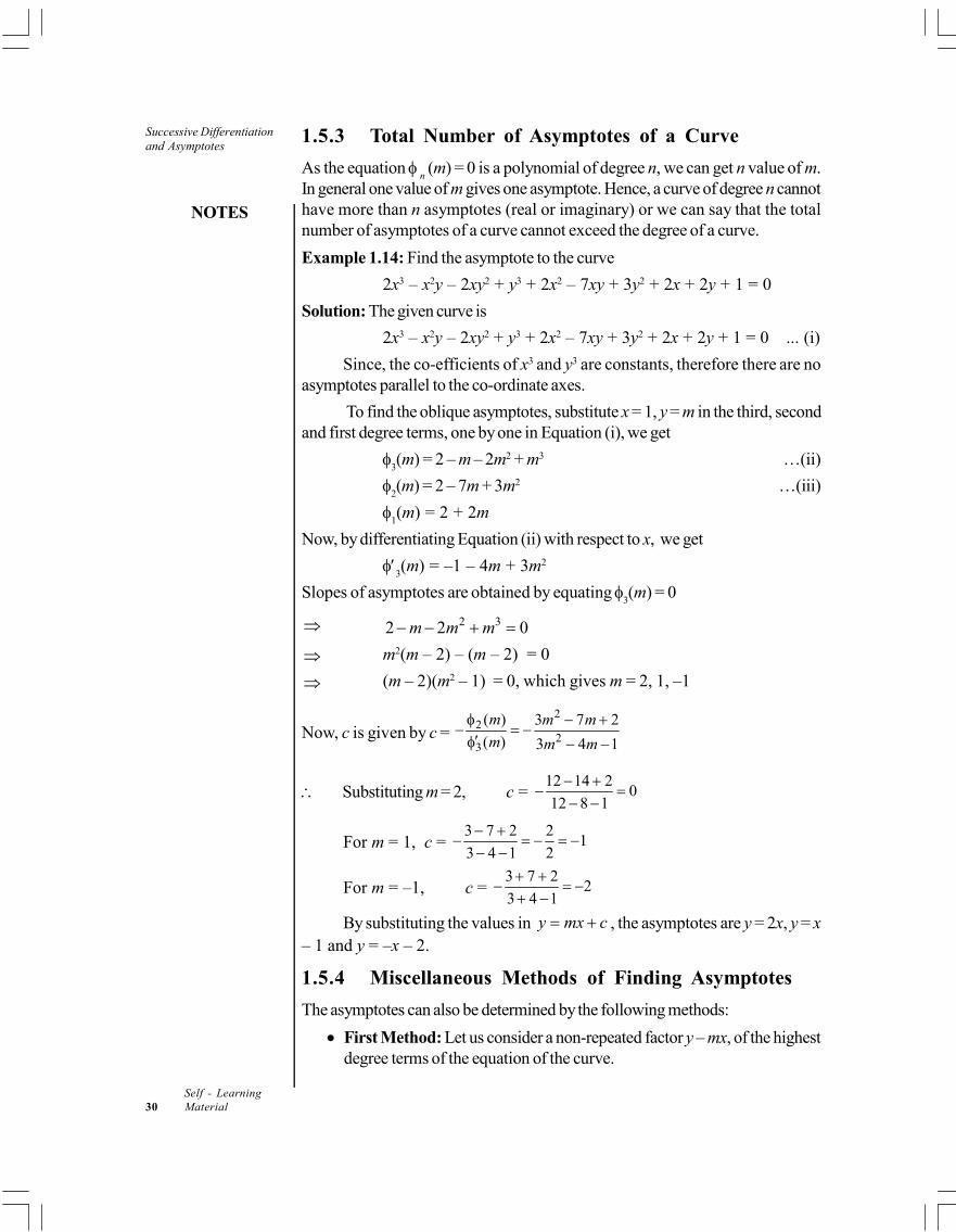
As the equation n (m) = 0 is a polynomial of degree n, we can get n value of m.
In general one value of m gives one asymptote. Hence, a curve of degree n cannothave more than n asymptotes (real or imaginary) or we can say that the totalnumber of asymptotes of a curve cannot exceed the degree of a curve.
Example 1.14: Find the asymptote to the curve
2x3 – x2y – 2xy2 + y3 + 2x2 – 7xy + 3y2 + 2x + 2y + 1 = 0
Solution: The given curve is
2x3 – x2y – 2xy2 + y3 + 2x2 – 7xy + 3y2 + 2x + 2y + 1 = 0 ... (i)
Since, the co-efficients of x3 and y3 are constants, therefore there are noasymptotes parallel to the co-ordinate axes.
To find the oblique asymptotes, substitute x = 1, y = m in the third, secondand first degree terms, one by one in Equation (i), we get
3(m) = 2 – m – 2m2 + m3 …(ii)
2(m) = 2 – 7m + 3m2 …(iii)
1(m) = 2 + 2m
Now, by differentiating Equation (ii) with respect to x, we get
3(m) = –1 – 4m + 3m2
Slopes of asymptotes are obtained by equating 3(m) = 0
2 32 2 0m m m
m2(m – 2) – (m – 2) = 0
(m – 2)(m2 – 1) = 0, which gives m = 2, 1, –1
Now, c is given by c = 2
22
3
( ) 3 7 2
( ) 3 4 –1
m m m
m m m
Substituting m = 2, c = 12 14 2
012 8 1
For m = 1, c = 3 7 2 2
13 4 1 2
For m = –1, c = 3 7 2
23 4 1
By substituting the values in y mx c , the asymptotes are y = 2x, y = x– 1 and y = –x – 2.
1.5.4 Miscellaneous Methods of Finding Asymptotes
The asymptotes can also be determined by the following methods:
First Method: Let us consider a non-repeated factor y – mx, of the highestdegree terms of the equation of the curve.
NOTES
Successive Differentiationand Asymptotes
Self - LearningMaterial 31
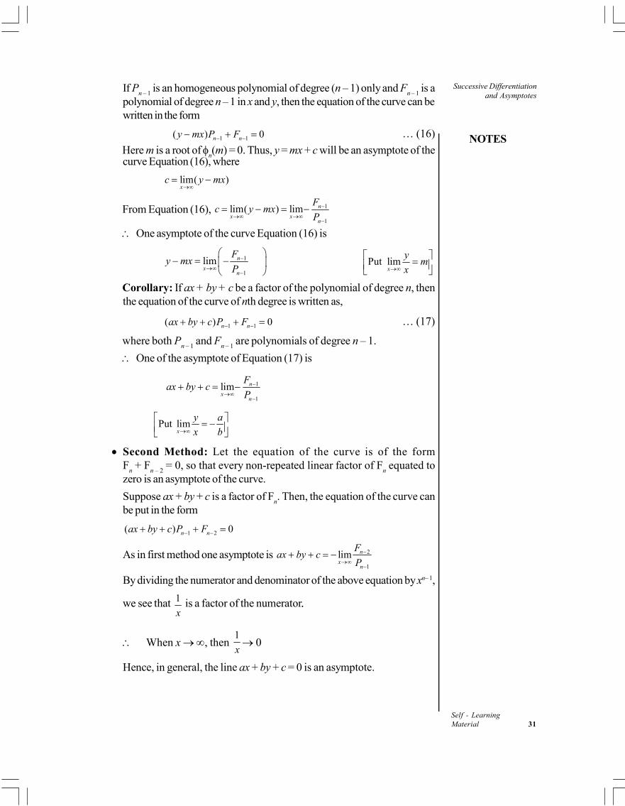
If Pn – 1
is an homogeneous polynomial of degree (n – 1) only and Fn – 1
is apolynomial of degree n – 1 in x and y, then the equation of the curve can bewritten in the form
1 1( ) 0n ny mx P F … (16)
Here m is a root of n(m) = 0. Thus, y = mx + c will be an asymptote of the
curve Equation (16), where
lim( )x
c y mx
From Equation (16), 1
1
lim( ) lim n
x xn
Fc y mx
P
One asymptote of the curve Equation (16) is
1
1
lim n
xn
Fy mx
P
Put lim
x
ym
x
Corollary: If ax + by + c be a factor of the polynomial of degree n, thenthe equation of the curve of nth degree is written as,
1 1( ) 0n nax by c P F … (17)
where both Pn – 1
and Fn – 1
are polynomials of degree n – 1.
One of the asymptote of Equation (17) is
1
1
lim n
xn
Fax by c
P
Put limx
y a
x b
Second Method: Let the equation of the curve is of the formF
n + F
n – 2 = 0, so that every non-repeated linear factor of F
n equated to
zero is an asymptote of the curve.
Suppose ax + by + c is a factor of Fn. Then, the equation of the curve can
be put in the form
1 2( ) 0n nax by c P F
As in first method one asymptote is 2
1
lim n
xn
Fax by c
P
By dividing the numerator and denominator of the above equation by xn– 1,
we see that 1
x is a factor of the numerator..
When x , then 1
x 0
Hence, in general, the line ax + by + c = 0 is an asymptote.
Successive Differentiationand Asymptotes
NOTES
Self - Learning32 Material
But if (ax + by + c)2 is a factor of Fn , then there will be two parallel
asymptotes given by
2 2
2
lim n
xn
Fax by c
P
.
Third Method: Let (y – mx)2 is a factor of the highest degree terms of theequation of the curve.
So, the equation of the curve is written as
22 1( ) 0n ny mx P F … (18)
We see that here no asymptote exists corresponding to the repeated factor(y – mx).
If (y – mx) is also a factor of terms of (n – 1)th degree of the equation of thecurve, then the equation of the curve is written as
22 2 2( ) ( ) 0n n ny mx P y mx F G
where Pn – 2
, Fn – 2
and Gn – 2
are the polynomial of degree n – 2, then theasymptote parallel to y – mx = 0 are given by
2 2 2
2 2
( ) ( ) lim lim 0n n
x xn n
F Gy mx y mx
P P
1.5.5 Intersection of a Curve and Its Asymptotes
Theorem 1.3: Any asymptote of an algebraic curve of nth degree cuts the curvein (n – 2) points.
Proof: Let y = mx + c … (19)
be an asymptote of the curve given by
1 21 2 ... 0n n n
n n n
y y yx x x
x x x
… (20)
Now, eliminating y from Equations (19) and (20), the abscissae of the pointsof intersection are given by
1 21 2 ... 0n n n
n n n
c c cx m x m x m
x x x
Expanding each term by Taylor’s theorem and arranging in descendingpowers of x, we get
1 21 2( ) '( ) ( )] ''( ) '( ) ( ) ... 0
2n n n
n n n n n n
cx m x c m m x m c m m
… (21)
Since, Equation (19) is an asymptote of (20), the coefficients of xn andxn–1 are both zero.
m and c are given by the equations
n(m) = 0 and c
n(m) +
n–1(m) = 0
NOTES
Successive Differentiationand Asymptotes
Self - LearningMaterial 33
Putting these values in Equation (21), we get
2 32''( ) '( ) ( ) [...] ... 0
2n n
n n n
cx m c m m x
which is of degree (n – 2) and this gives (n – 2) values of x.
Hence an asymptote of a curve of nth degree cuts the curve in (n – 2) points.
Cor. I: If a curve of nth degree has n asymptotes, then the point of intersection ofa curve and its asymptotes are n(n – 2).
Cor. II: Let the joint equation of n asymptotes be given by
Fn = 0 … (22)
and the equation of the curve be F
n + F
n – 2 = 0 … (23)
The Equations (22) and (23) hold simultaneously at the points of intersection ofthe curve and its asymptotes. Hence for such points, we have
Fn – 2
= 0
Thus, Fn – 2
= 0 is a curve on which lie all the points of intersection of thecurve and its asymptotes.
Example 1.15: Show that the point of intersection of the curve
3 2 2 3 2 22 2 4 4 14 6 4 6 1y x y xy x xy y x y = 0
and its asymptotes lie on the straight line 8x + 2y + 1 = 0
Solution: The equation of the given curve is
3 2 2 3 2 22 2 4 4 14 6 4 6 1y x y xy x xy y x y = 0 …(i)
The curve has no asymptotes parallel to x-axis or y-axis.
( the co-efficients of 3x and 3y , the highest degree terms in x and y are constants)
To obtain the oblique asymptote, substitute x = 1, y = m in the two highest (i.e.,third and second) degree terms
( )n m = 3 ( )m = 3 22 2 4 4m m m
and 1( )n m = 2 ( )m = 214 6 4m m
The slopes of the asymptotes are given by ( )n m = 0 3 ( ) 0m
3 22 2 4 4m m m = 0
2 22 ( 1) 4 ( 1)m m m = 0
2(2 4) ( 1)m m = 0
m = 2, 1, –1
Successive Differentiationand Asymptotes
NOTES
Self - Learning34 Material
Also ( )n m = 3 ( )m = 26 2 8m m
c = 1 ( )
( )n
n
m
m
=
2
3
( )
( )
m
m
= 2
2
( 14 6 4)
6 2 8
m m
m m
= 2
2
7 3 2
3 4 1
m m
m m
When m = 2, c = 14 12 2
12 8 1
= 0,
When m = 1, c = 7 3 2
3 4 1
= 2
2 = – 1.
When m = – 1,
c = 7 3 2
3 4 1
= – 2
Putting these values of m and c in y = mx + c, the asymptotes arey = 2x + 0, y = x – 1, and y = –x –2
2x – y = 0, x – y – 1 = 0 and x + y + 2 = 0.Thus, the three asymptotes will cut the curve again in 3(3 – 2) = 3 points.The joint equation of the asymptotes is
(2 ) ( 1) ( 2)x y x y x y = 0
3 2 2 3 2 22 2 7 3 2 2 4y x y xy x xy y x y x = 0
Multiplying by 23 2 2 3 2 22 2 4 4 14 6 4 4 8y x y xy x xy y x y x = 0.
Now the equation of the curve is3 2 2 3 2 22 2 4 4 14 6 4 6 1y x y xy x xy y x y = 0
which can be re-written as3 2 2 3 2 2[2 2 4 4 14 6 4 4 8 ] [2 8 1]y x y xy x xy y x y x y x = 0
which is of the form 2F Fn n = 0
Hence, the points of intersection lie on the curve
2Fn = 0 or 2 8 1y x = 0 or 8 2 1x y = 0
which is the required straight line.
1.5.6 Asymptotes of Polar Curves
Theorem 1.4: If the equation of the polar curve be r = f(), then the equation ofthe asymptote is given by
P sin( )r
NOTES
Successive Differentiationand Asymptotes
Self - LearningMaterial 35
where 1P lim
du
du r
and is a root of the equation obtained by putting
u = 0 (Refer Figure 1.5).
O
L
T’
X
P
– /2
T
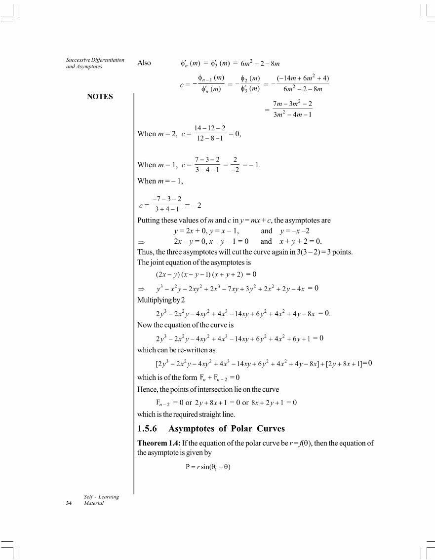
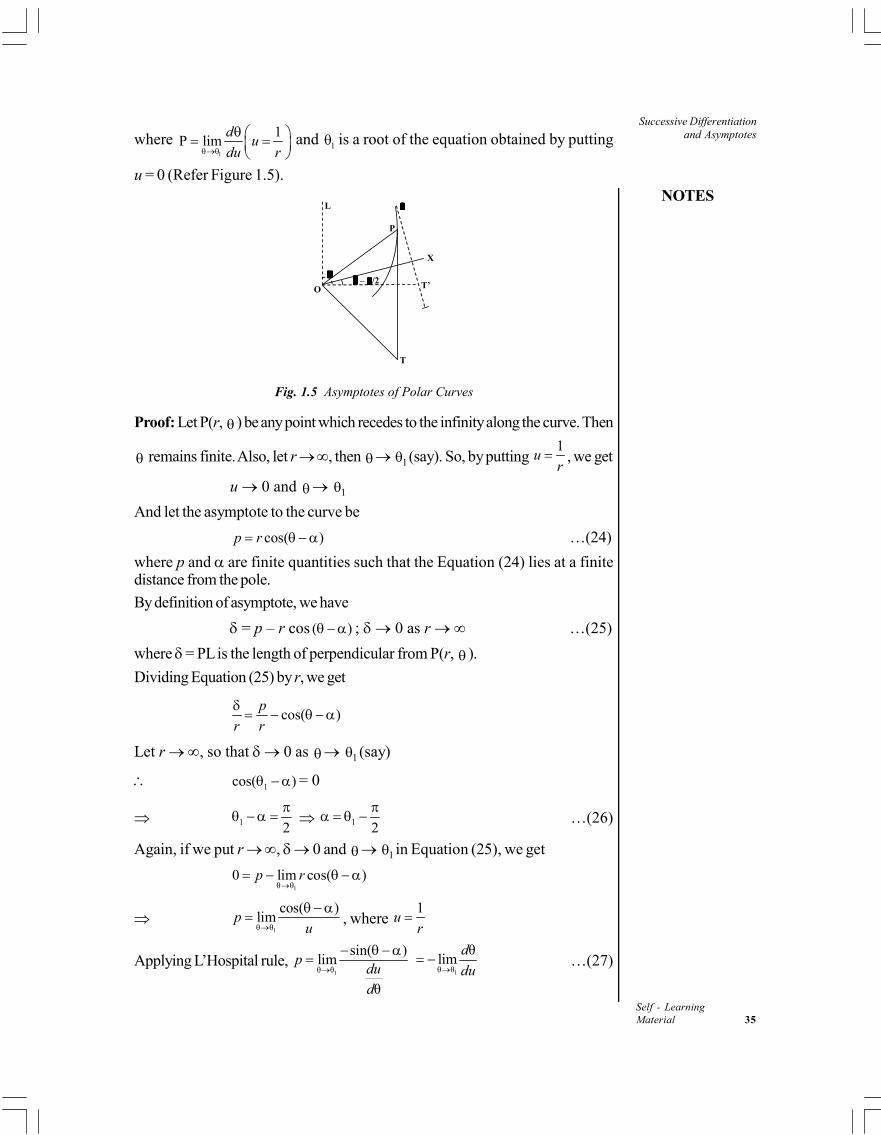
Fig. 1.5 Asymptotes of Polar Curves
Proof: Let P(r, ) be any point which recedes to the infinity along the curve. Then
remains finite. Also, let r , then 1 (say). So, by putting 1
ur
, we get
u 0 and 1
And let the asymptote to the curve be
cos( )p r …(24)
where p and are finite quantities such that the Equation (24) lies at a finitedistance from the pole.
By definition of asymptote, we have
= p – r cos ( ) ; 0 as r …(25)
where = PL is the length of perpendicular from P(r, ).
Dividing Equation (25) by r, we get
cos( )p
r r
Let r , so that 0 as 1 (say)
1cos( ) = 0
1
1
…(26)
Again, if we put r , 0 and 1 in Equation (25), we get
1θ θ0 lim cos( )p r
1θ θ
cos( )limp
u
, where
1u
r
Applying L’Hospital rule, 1θ θ
sin( )lim
θ
pdu
d
1θ θ
θlim
d
du …(27)
Successive Differentiationand Asymptotes
NOTES
Self - Learning36 Material
By putting the values of p and from Equations (27) and (26), respectively inEquation (24), we get
1
1 1θ θ
θ πlim cos θ θ sin θ θ
2
dr r
du
11
θ θ
θlim sin θ θ
dr
du
This is the required equation of the asymptote in polar co-ordinates.
Working Rule for Finding Asymptotes of Polar Curves
1. Put r = 1
uin the given equation.
2. If the given equation has trigonometric ratios, convert them to sin andcos . Find the limit of as u 0. Let
1,
2, ……
n be the limits
obtained.
3. Find p = 0
lim –i
u
d
du
for each of the i, obtained in step 2.
4. The corresponding asymptotes are given by the equation p = r sin (i – ).
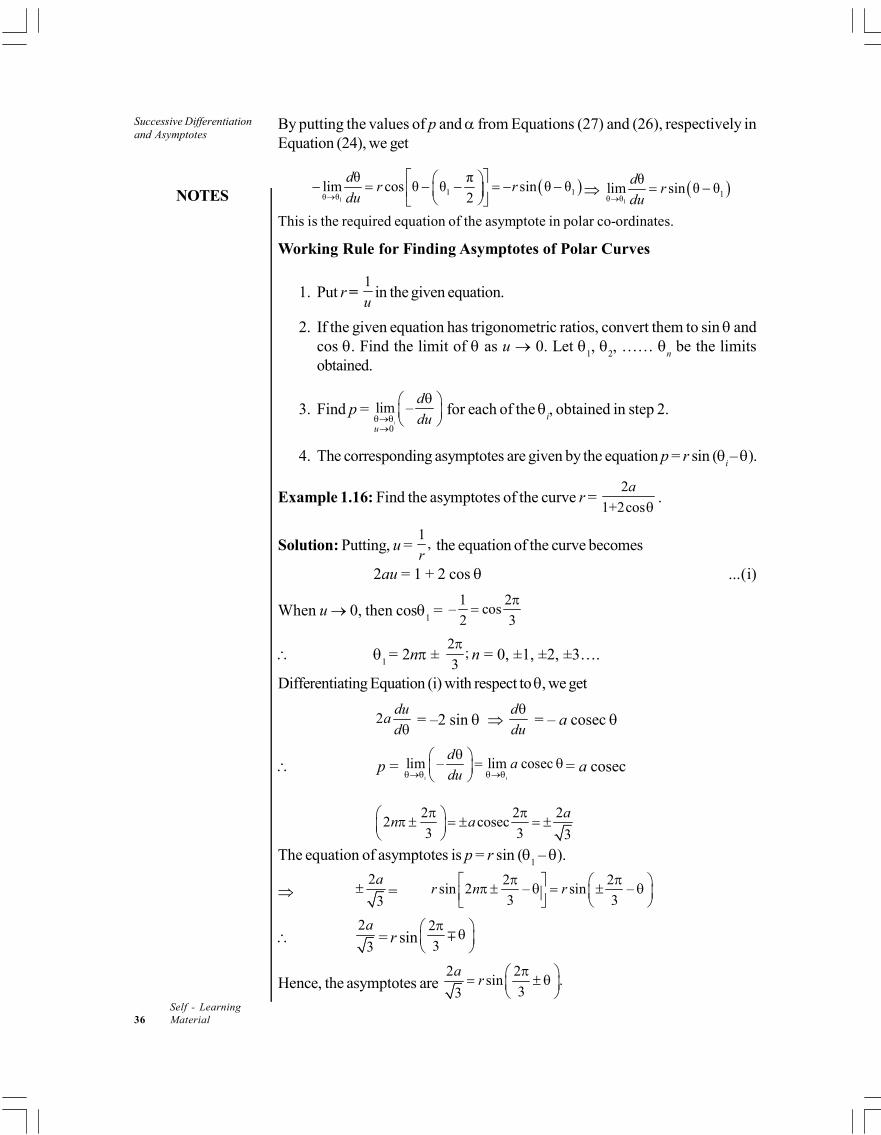
Example 1.16: Find the asymptotes of the curve r = 2
1+2cos
a
.
Solution: Putting, u = 1
,r
the equation of the curve becomes
2au = 1 + 2 cos i
When u 0, then cos1 =
1 2– cos
2 3
1 = 2n ±
2;
3
n = 0, ±1, ±2, ±3….
Differentiating Equation (i) with respect to , we get
2du
ad
= –2 sin d
du
= –a cosec
p = 1 1
lim – lim cosecd
adu
= a cosec
2 2 22 cosec
3 3 3
an a
The equation of asymptotes is p = r sin (1 – ).
2
3
a =
2 2sin 2 – sin –
3 3r n r
2
3
a= r sin
2
3
Hence, the asymptotes are 2 2
sin .33
ar
NOTES
Successive Differentiationand Asymptotes
Self - LearningMaterial 37
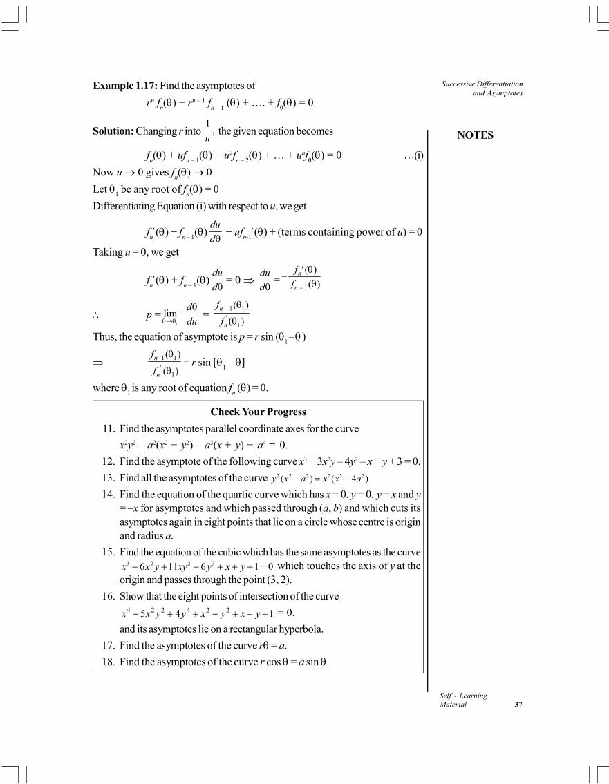
Example 1.17: Find the asymptotes of
rn fn() + rn – 1 f
n – 1 () + …. + f
0() = 0
Solution: Changing r into 1
,u
the given equation becomes
fn() + uf
n – 1() + u2f
n – 2() + … + unf
0() = 0 …(i)
Now u 0 gives fn() 0
Let 1 be any root of f
n() = 0
Differentiating Equation (i) with respect to u, we get
fn() + f
n – 1()
du
d + uf
n-1() + (terms containing power of u) = 0
Taking u = 0, we get
fn() + f
n – 1()
du
d= 0
du
d=
– 1
( )–
( )n
n
f
f
p =1
limd
du
=
– 1 1
1
( )
( )n
n
f
f
Thus, the equation of asymptote is p = r sin (1 – )
–1 1
1
( )
( )
n
n
f
f
= r sin [1 – ]
where 1 is any root of equation f
n () = 0.
Check Your Progress
11. Find the asymptotes parallel coordinate axes for the curve
x2y2 – a2(x2 + y2) – a3(x + y) + a4 = 0.
12. Find the asymptote of the following curve x3 + 3x2y – 4y2 – x + y + 3 = 0.
13. Find all the asymptotes of the curve 2 2 2 2 2 2( ) ( 4 )y x a x x a
14. Find the equation of the quartic curve which has x = 0, y = 0, y = x and y= –x for asymptotes and which passed through (a, b) and which cuts itsasymptotes again in eight points that lie on a circle whose centre is originand radius a.
15. Find the equation of the cubic which has the same asymptotes as the curve3 2 2 36 11 6 1 0x x y xy y x y which touches the axis of y at the
origin and passes through the point (3, 2).
16. Show that the eight points of intersection of the curve4 2 2 4 2 25 4 1x x y y x y x y = 0.
and its asymptotes lie on a rectangular hyperbola.
17. Find the asymptotes of the curve r = a.
18. Find the asymptotes of the curve r cos = a sin .
Successive Differentiationand Asymptotes
NOTES
Self - Learning38 Material
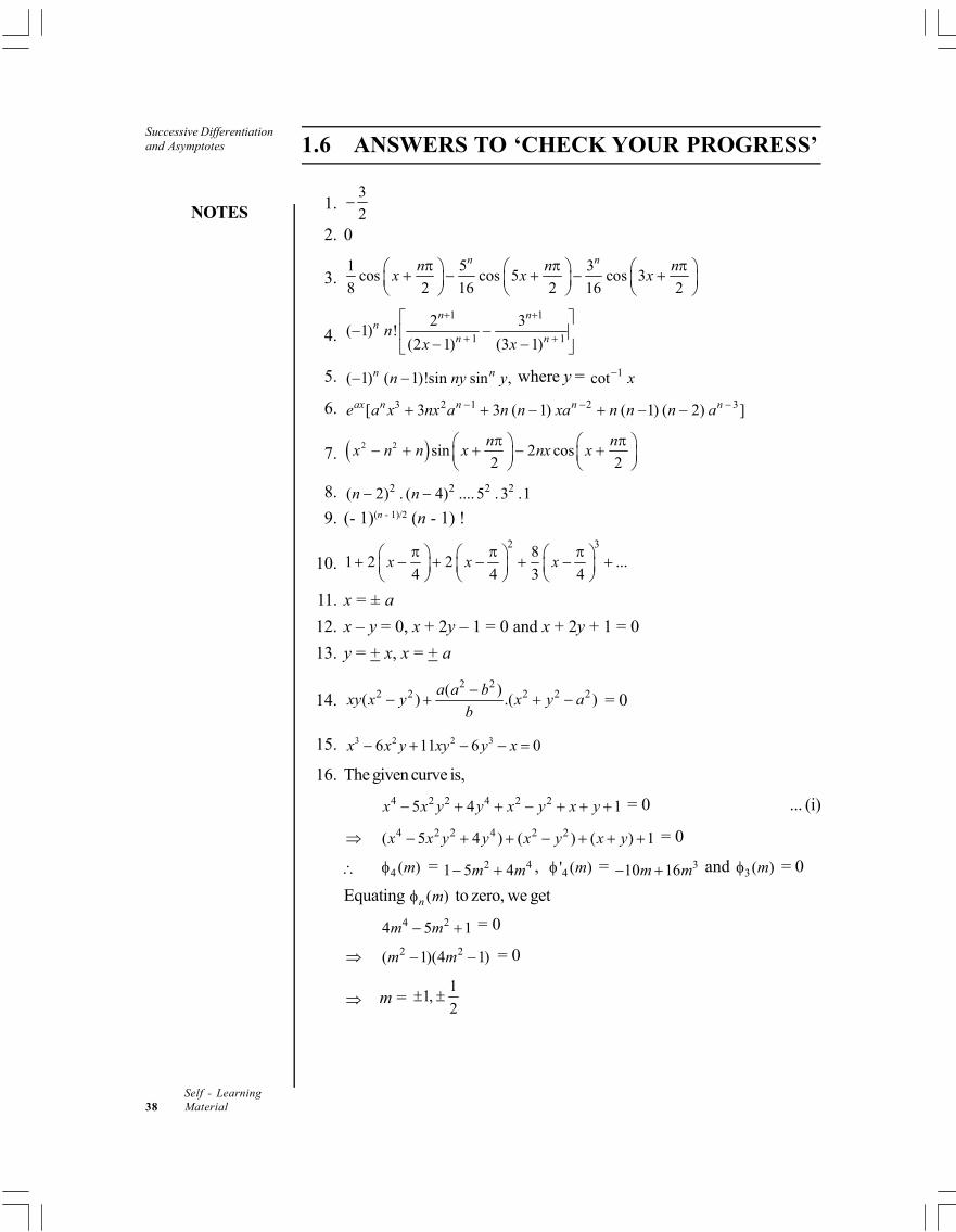
1.6 ANSWERS TO ‘CHECK YOUR PROGRESS’
1.3
2
2. 0
3.1 5 3
cos cos 5 cos 38 2 16 2 16 2
n nn n nx x x
4.1 1
1 1
2 3( 1) ! .
(2 1) (3 1)
n nn
n nn
x x
5. ( 1) ( 1)!sin sin ,n nn ny y where y = 1cot x
6. 3 2 1 2 3[ 3 3 ( 1) ( 1) ( 2) ]ax n n n ne a x nx a n n xa n n n a
7. 2 2 sin 2 cos .2 2
n nx n n x nx x
8. 2 2 2 2( 2) . ( 4) .... 5 . 3 .1.n n
9. (- 1)(n - 1)/2 (n - 1) !
10.2 3
81 2 2 ...
4 4 3 4x x x
11. x = ± a
12. x – y = 0, x + 2y – 1 = 0 and x + 2y + 1 = 0
13. y = + x, x = + a
14.2 2
2 2 2 2 2( )( ) .( )
a a bxy x y x y a
b
= 0
15. 3 2 2 36 11 6 0x x y xy y x
16. The given curve is,
4 2 2 4 2 25 4 1x x y y x y x y = 0 ... (i)
4 2 2 4 2 2( 5 4 ) ( ) ( ) 1x x y y x y x y = 0
4 ( )m = 2 41 5 4m m , 4' ( )m = 310 16m m and 3( )m = 0
Equating ( )n m to zero, we get
4 24 5 1m m = 0
2 2( 1)(4 1)m m = 0
m = 1
1,2
NOTES
Successive Differentiationand Asymptotes
Self - LearningMaterial 39
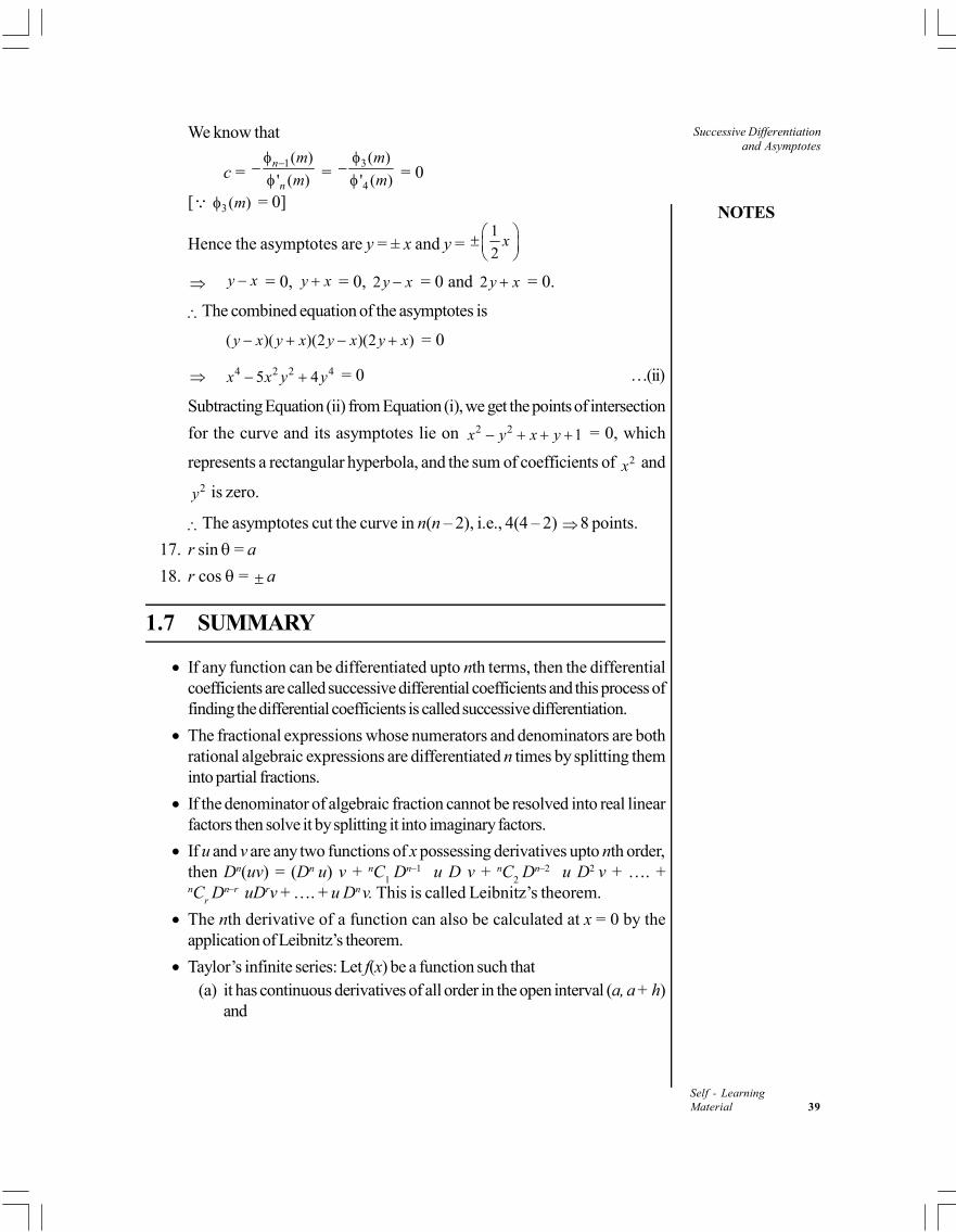
We know that
c = 1( )
' ( )n
n
m
m
=
3
4
( )
' ( )
m
m
= 0
[ 3( )m = 0]
Hence the asymptotes are y = ± x and y = 1
2x
y x = 0, y x = 0, 2y x = 0 and 2y x = 0.
The combined equation of the asymptotes is
( )( )(2 )(2 )y x y x y x y x = 0
4 2 2 45 4x x y y = 0 …(ii)
Subtracting Equation (ii) from Equation (i), we get the points of intersection
for the curve and its asymptotes lie on 2 2 1x y x y = 0, which
represents a rectangular hyperbola, and the sum of coefficients of 2x and
2y is zero.
The asymptotes cut the curve in n(n – 2), i.e., 4(4 – 2) 8 points.
17. r sin = a
18. r cos = a
1.7 SUMMARY
If any function can be differentiated upto nth terms, then the differentialcoefficients are called successive differential coefficients and this process offinding the differential coefficients is called successive differentiation.
The fractional expressions whose numerators and denominators are bothrational algebraic expressions are differentiated n times by splitting theminto partial fractions.
If the denominator of algebraic fraction cannot be resolved into real linearfactors then solve it by splitting it into imaginary factors.
If u and v are any two functions of x possessing derivatives upto nth order,then Dn(uv) = (Dn u) v + nC
1 Dn–1 u D v + nC
2 Dn–2 u D2 v + …. +
nCr Dn–r uDrv + …. + u Dn v. This is called Leibnitz’s theorem.
The nth derivative of a function can also be calculated at x = 0 by theapplication of Leibnitz’s theorem.
Taylor’s infinite series: Let f(x) be a function such that(a) it has continuous derivatives of all order in the open interval (a, a + h)
and
Successive Differentiationand Asymptotes
NOTES
Self - Learning40 Material
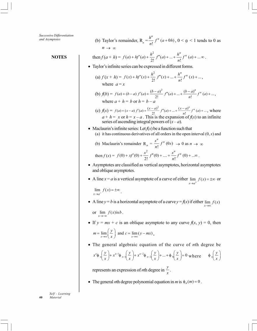
(b) Taylor’s remainder, Rn = ( )
!
nnh
f a hn
, 0 < < 1 tends to 0 as
n
then f (a + h) = 2
( ) ( ) ( ) ... ( ) ...2! !
nnh h
f a hf a f a f an
.
Taylor’s infinite series can be expressed in different forms.
(a) f (x + h) = 2
( ) ( ) ( ) ... ( ) ...2! !
nnh h
f x hf x f x f xn
,
where a = x
(b) f(b) = 2( ) ( )
( ) ( ) ( ) ( ) ... ( ) ...2! !
nnb a b a
f a b a f a f a f an
,
where a + h = b or h = b – a
(c) f(x) = 2( ) ( )
( ) ( ) ( ) ( ) ... ( ) ...2! !
nnx a x a
f a x a f a f a f an
, where
a + h = x or h = x – a . This is the expansion of f(x) to an infiniteseries of ascending integral powers of (x – a).
Maclaurin’s infinite series: Let f(x) be a function such that(a) it has continuous derivatives of all orders in the open interval (0, x) and
(b) Maclaurin’s remainder Rn = ( )!
nnx
f xn
0 as n
then f (x) = 2
(0) (0) (0) .... (0) ...2! !
nnx x
f xf f fn
.
Asymptotes are classified as vertical asymptotes, horizontal asymptotesand oblique asymptotes.
A line x = a is a vertical asymptote of a curve of either lim ( )x a
f x
or
lim ( )x a
f x
.
A line y = b is a horizontal asymptote of a curve y = f(x) if either lim ( )x
f x
or lim ( )isx
f x b
.
If y = mx + c is an oblique asymptote to any curve f(x, y) = 0, then
lim and lim ( )x x
ym c y mx
x
.
The general algebraic equation of the curve of nth degree be
1 21 2 0... 0n n n
n n n
y y y yx x x
x x x x
where n
y
x
represents an expression of nth degree in y
x.
The general nth degree polynomial equation in m is ( ) 0n m .
NOTES
Successive Differentiationand Asymptotes
Self - LearningMaterial 41
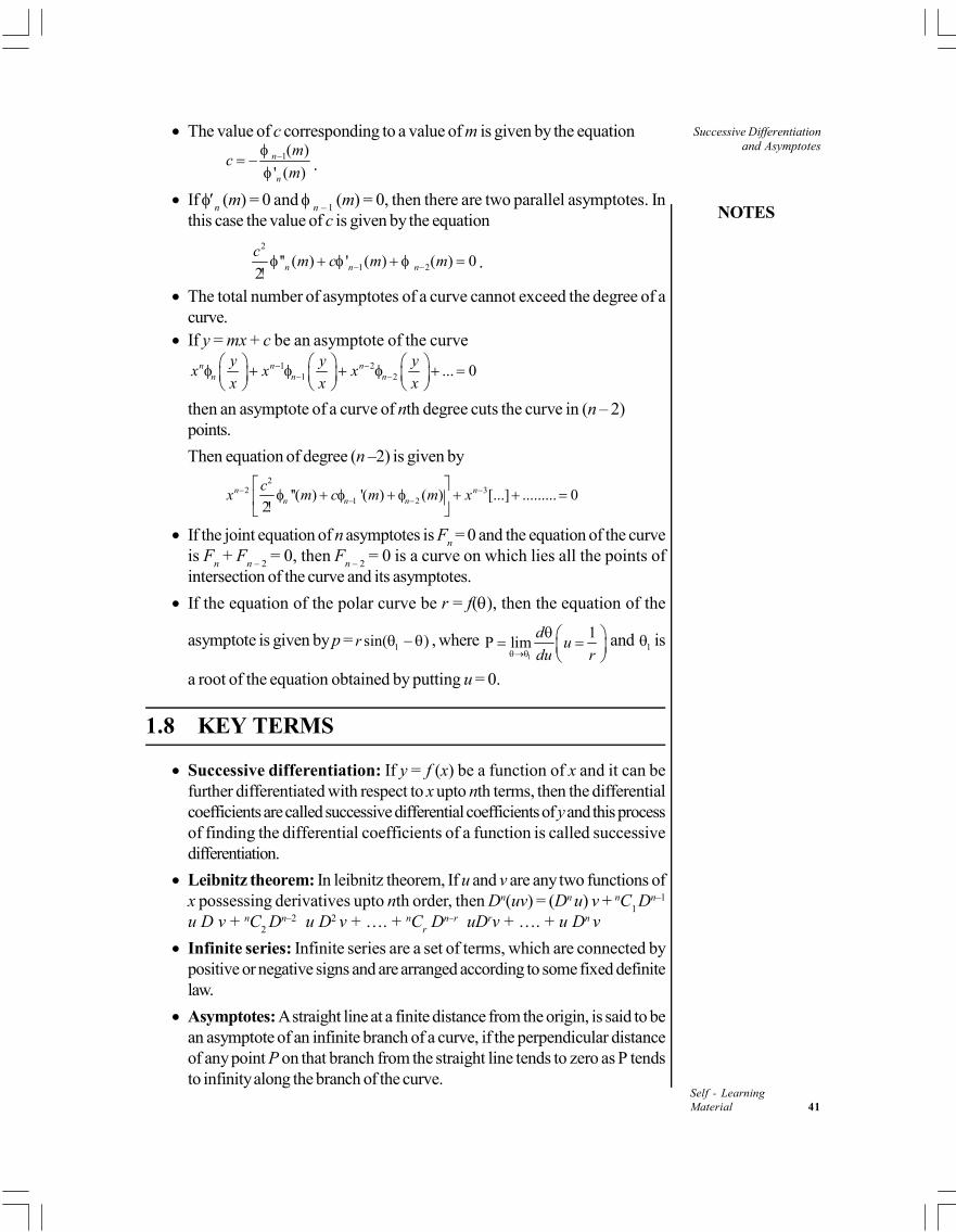
The value of c corresponding to a value of m is given by the equation1( )
' ( )n
n
mc
m
.
If n (m) = 0 and
n – 1
(m) = 0, then there are two parallel asymptotes. Inthis case the value of c is given by the equation
2
1 2'' ( ) ' ( ) ( ) 02 n n n
cm c m m
.
The total number of asymptotes of a curve cannot exceed the degree of acurve.
If y = mx + c be an asymptote of the curve1 2
1 2 ... 0n n nn n n
y y yx x x
x x x
then an asymptote of a curve of nth degree cuts the curve in (n – 2)points.
Then equation of degree (n –2) is given by
2 32''( ) '( ) ( ) [...] ......... 0
2n n
n n n
cx m c m m x
If the joint equation of n asymptotes is Fn = 0 and the equation of the curve
is Fn + F
n – 2 = 0, then F
n – 2 = 0 is a curve on which lies all the points of
intersection of the curve and its asymptotes.
If the equation of the polar curve be r = f(), then the equation of the
asymptote is given by p = sin( )r , where 1P lim
du
du r
and is
a root of the equation obtained by putting u = 0.
1.8 KEY TERMS
Successive differentiation: If y = f (x) be a function of x and it can befurther differentiated with respect to x upto nth terms, then the differentialcoefficients are called successive differential coefficients of y and this processof finding the differential coefficients of a function is called successivedifferentiation.
Leibnitz theorem: In leibnitz theorem, If u and v are any two functions ofx possessing derivatives upto nth order, then Dn(uv) = (Dn u) v + nC
1 Dn–1
u D v + nC2 Dn–2 u D2 v + …. + nC
r Dn–r uDrv + …. + u Dn v
Infinite series: Infinite series are a set of terms, which are connected bypositive or negative signs and are arranged according to some fixed definitelaw.
Asymptotes: A straight line at a finite distance from the origin, is said to bean asymptote of an infinite branch of a curve, if the perpendicular distanceof any point P on that branch from the straight line tends to zero as P tendsto infinity along the branch of the curve.
Successive Differentiationand Asymptotes
NOTES
Self - Learning42 Material
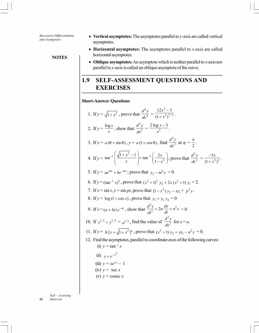
Vertical asymptotes: The asymptotes parallel to y-axis are called verticalasymptotes.
Horizontal asymptotes: The asymptotes parallel to x-axis are calledhorizontal asymptotes.
Oblique asymptotes: An asymptote which is neither parallel to x-axis norparallel to y-axis is called an oblique asymptote of the curve.
1.9 SELF-ASSESSMENT QUESTIONS ANDEXERCISES
Short-Answer Questions
1. If y = 21 x , prove that 4
4
d y
dx =
2
2 7 / 2
12 3
(1 )
x
x
.
2. If y = log x
x, show that
2
2
d y
dx = 3
2 log 3x
x
.
3. If x = ( sin )a , y = (1 cos )a , find 2
2
d y
dx at =
2
.
4. If y = 2
1 12
1 1 2tan tan
1
x x
x x
; prove that 2
2
d y
dx = 2 2
5
(1 )
x
x
.
5. If y = mx mxae be ; prove that 22y m y = 0.
6. If y = 1 2(tan )x , prove that 2 2 22 1( 1) 2 ( 1)x y x x y = 2.
7. If x = sin t, y = sin pt, prove that 22 1(1 )x y xy + 2p y .
8. If y = log (1 cos )x , prove that 3 1 2y y y = 0
9. If x = ( ) nta bt e , show that 2
22
2d x dx
n n xdtdt
= 0
10. If 1/ 2 1/ 2x y = 1/ 2a , find the value of 2
2
d y
dx for x = a.
11. If y = 2A [ 1 ]nx x , prove that 2 22 1( 1)x y xy n y = 0.
12. Find the asymptotes, parallel to coordinate axes of the following curves:(i) y = tan–1 x
(ii) 2 xy e
(iii) y = xe1/x 1(iv) y = sec x(v) y = cosec x
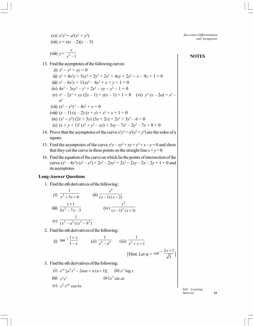
NOTES
Successive Differentiationand Asymptotes
Self - LearningMaterial 43
(vi) x2y2 = a2(x2 + y2)(vii) y = x(x – 2)(x – 3)
(viii) y = 2 –1
x
x
13. Find the asymptotes of the following curves:(i) x4 y4 + xy = 0(ii) x3 + 4x2y + 5xy2 + 2y3 + 2x2 + 4xy + 2y2 x 9y + 1 = 0(iii) x3 – 6x2y + 11xy2 – 6y3 + x + y + 1 = 0(iv) 4x3 – 3xy2 – y3 + 2x2 – xy y2 1 = 0(v) x3 – 2y3 + xy (2x – 1) + y(x – 1) + 1 = 0 (vi) y2 (x – 2a) = x3 –
a3
(vii) (x2 – y2) 2 – 4x2 + x = 0(viii) (x – 1) (x – 2) (x + y) + x2 + x + 1 = 0(ix) (x2 y2) (2x + 3y) (3x + 2y) + 2x2 + 3y2 – 6 = 0(x) (x + y + 1)2 (x2 + y2 – xy) + 3xy – 7x2 – 2y2 – 7x + 8 = 0
14. Prove that the asymptotes of the curve x2y2 = a2(x2 + y2) are the sides of asquare.
15. Find the asymptotes of the curve x2y – xy2 + xy + y2 + x – y = 0 and showthat they cut the curve in three points on the straight line x + y = 0.
16. Find the equation of the curve on which lie the points of intersection of thecurve (x2 – 4y2) (x2 – y2) + 2x3 – 2xy2 + 2x2 – 2xy – 2x – 2y + 1 = 0 andits asymptotes.
Long-Answer Questions
1. Find the nth derivatives of the following :
(i) 2
1
5 6x x (ii) 4
( 1) ( 2)
x
x x
(iii) 2
1
6 7 3
x
x x
(iv)
2
3( 1) ( 1)
x
x x
(v) 2 2 2 2
1
( ) ( )x a x b
2. Find the nth derivatives of the following :
(i)1 1
tan1
x
x
(ii) 4 4
1
x a (iii) 2
1
1x x
[Hint. Let = 1 2 1
cot3
x ]
3. Find the nth derivatives of the following:
(i) 2 2[ 2 ( 1)]axe a x nax n n (ii) logxe x
(iii) n xx e (iv) 3 sinx ax
(v) 2 cosaxx e bx
Successive Differentiationand Asymptotes
NOTES
Self - Learning44 Material
4. Find the nth derivative of
(i)2
2 22
(1 )d y dy
x x a ydxdx
= 0 (ii) 22 1x y xy y = 0.
5. If y = lognx x , show that 1ny = !n
x.
6. If y = 1tan x , prove that
(i) 22 1(1 ) 2x y xy = 0
(ii) 21 1(1 ) 2 ( 1)n n nx y nxy n n y = 0
7. If y = 1sinm xe prove that
(i) 22 1(1 )x y xy = 2m y
(ii) 2 2 22 1(1 ) (2 1) ( )n n nx y n xy n m y = 0.
8. If y = 1cosm xe , prove that 2 2 2
2 1(1 ) (2 1) ( )n n nx y n xy n m y = 0.
9. If y = 2( 1)nx , prove that 22 1( 1) 2 ( 1)n n nx y xy n n y = 0.
10. If 1cos
y
b
= logn
x
n
; prove that 2 22 1(2 1) 2n n nx y n xy n y = 0.
11. If y =
1
2
sin
1
x
x
, prove that 2 22 1(1 ) (2 3) ( 1)n n nx y n xy n y = 0.
12. If y = 1 2(sin ) ,h x prove that 2 22 1(1 ) (2 1)n n nx y n xy n y = 0.
Also find (0)ny .
13. Show by means of Maclaurin’s infinite series expansion that:
(i) 1tan (1 )x = 2 3
...4 2 4 12
x x x
(ii)2 4
log (1 ) log 2 ...2 8 192
xe
x x xe
(iii) esinx = 2 43
1 ...1.2 1.2.3.4
x xx
(iv)2 32 4
1 ...cos 2! 3!
xe x xx
x
(v) log cos x = 2 4 62 16
...2! 4! 6!
x x x
14. Prove that:
(i)2 3 42 7
log(1 tan ) ...2 3 12
x x xx x
NOTES
Successive Differentiationand Asymptotes
Self - LearningMaterial 45
(ii)2
1 1 1tan
x
x
= 3 5 71
...2 3 5 7
x x xx
(iii)2
14
2sin
1
x
x
= 6 10
22 ...3 5
x xx
(iv) 2log (1 )x x = 2 3 4 5 6 7 82 2
...2 3 4 5 6 7 8
x x x x x x xx
15. Expand the following by Maclaurin’s infinite series expansion in the powersof x as far as the term containing x3
(i) secxe x
(ii) log(1 )xe x
(iii) log [1 + log (1 + x)](iv) log [1 – log (1 – x)]
16. Expand sinaxe bx as an infinite series of ascending powers of x. Give also
the (n + 1) term of the series.
17. Expand 2log (1 sin )x in powers of x as far as terms containing 4x .
18. Find the approximate value of 26 to three decimal places by Taylor’ssexpansion.
19. Expand the following:
(i) xa in powers of (x – a)
(ii) log x in powers of (x – k)
(iii) 24 7 5x x in powers of (x + 2)
(iv) 1tan x in the powers of4
x
20. Prove that
22 1( ) '( ) . ''( ) ...
1 1 1 2
x x xf f x f x f x
x x x
21. Find the asymptotes of the curve xy(x2 – y2) + x2 + y2 – a2 = 0. Show thatthe eight points of intersection of the curve with its asymptotes lie on a circlewhose centre is at the origin.
22. Find all the asymptotes of curve (x + y + 1) (y + 2x + 2) (y + 3x + 3)(y – x) + x2 + y2 – 8x = 0 and show that the eight points of intersection ofthe curve and its asymptotes lie on a circle. Find also the centre and theradius of the circle.
23. Find the equation of the cubic which has the same asymptotes as the curve
x3 – 6x2y – 11xy2 – 6y3 + x + y + 4 = 0 and which passes through (0, 0),(2, 0) and (0, 2).
Successive Differentiationand Asymptotes
NOTES
Self - Learning46 Material
24. Find the asymptotes of the following curves:(i) r2 = a2
(ii) r = 1
a
(iii) r = 1 cos
a
(iv) r = 2
1 2cos
a
(v) r(1 – e) = a(vi) r( + ) = ae(vii) r log = a(viii) r cos = a cos 2(ix) r cos = a cos2(x) r cos = a sin2 (xi) r = a cosec + b cot (xii) r = a + b cot n(xiii) r2 = a2(sec2 + cosec2 )
(xiv) r = 3 3
3 sin cos
sin cos
a
(xv) rn sin n = an
1.10 FURTHER READING
Prasad, Gorakh. 2016. Differential Calculus. Allahabad: Pothishala Private Ltd.
Prasad, Gorakh. 2015. Integral Calculus. Allahabad: Pothishala Private Ltd.
Murray, Daniel A. 1967. Introductory Course in Differential Equations. India:Orient Longman.
Coddington, Earl A. 1987. An Introduction to Ordinary Differential Equations.New Delhi: Prentice Hall of India.
Coddington, Earl A. and N. Levinson. 1972. Theory of Ordinary DifferentialEquations. New Delhi: Tata Mc Graw-Hill.
Boyce, W.E. and Richard C. DiPrima. 1986. Elementary Differential Equationsand Boundary Value Problems. New York: John Wiley and Sons, Inc.
Gelfand, J.M. and S.V. Fomin. 1963. Calculus of Variations. New Jersey: PrenticeHall.
Ross, S. L. 1984. Differential Equations, 3rd Edition. New York: John Wileyand Sons.
Somasundaram, D. 2002. Ordinary Differential Equations. Chennai: NarosaPublishing House.
NOTES
Curvature
Self - LearningMaterial 47
UNIT 2 CURVATURE
Structure
2.0 Introduction2.1 Objectives2.2 Curvature
2.2.1 Radius of Curvature for Cartesian Curves2.2.2 Radius of Curvature for Polar and Pedal Equations2.2.3 Radius of Curvature at the Origin2.2.4 Centre of Curvature2.2.5 Chord of Curvature
2.3 Tests for Concavity and Convexity2.4 Points of Inflection2.5 Multiple Points2.6 Tracing of Curves in Cartesian and Polar Coordinates2.7 Answers to ‘Check Your Progress’2.8 Summary2.9 Key Terms
2.10 Self-Assessment Questions and Exercises2.11 Further Reading
2.0 INTRODUCTION
In mathematics, curvature is any of several strongly related concepts in geometry.Spontaneously, the curvature is the amount by which a curve deviates from beinga straight line, or a surface deviates from being a plane. For curves, the canonicalexample is that of a circle, which has a curvature equal to the reciprocal of itsradius. Smaller circles bend more sharply, and hence have higher curvature.
The numerical measures of the sharpness of the bending of a curve at apoint is called the curvature of the curve at that point. Here, curvature of PA isgreater than that of PB. If we roughly regard PA and PB as arcs of circles then wesee that radius of PA is less than the radius of PB. Thus we can say that radius ofcircle would be small when curvature is large and vice-versa.
Curve tracing or curve sketching means how to draw the rough sketch ofthe given curve. Principally, curve tracing helps in finding the approximate shape ofa curve without plotting a large number of points. Mathematically, the term curvetracing includes techniques that can be used to produce a rough idea of overallshape of a plane curve given its equation without computing the large numbers ofpoints required for a detailed plot. Many properties of the curve can be determinedeasily by knowing its graph. The theory of curves method is typically used to tracea curve whose equation is given in Cartesian, polar or parametric equations.
In this unit, you will study about curvature, tests for concavity and convexity,points of inflection, multiple points, tracing of curves in Cartesian and polarcoordinates.
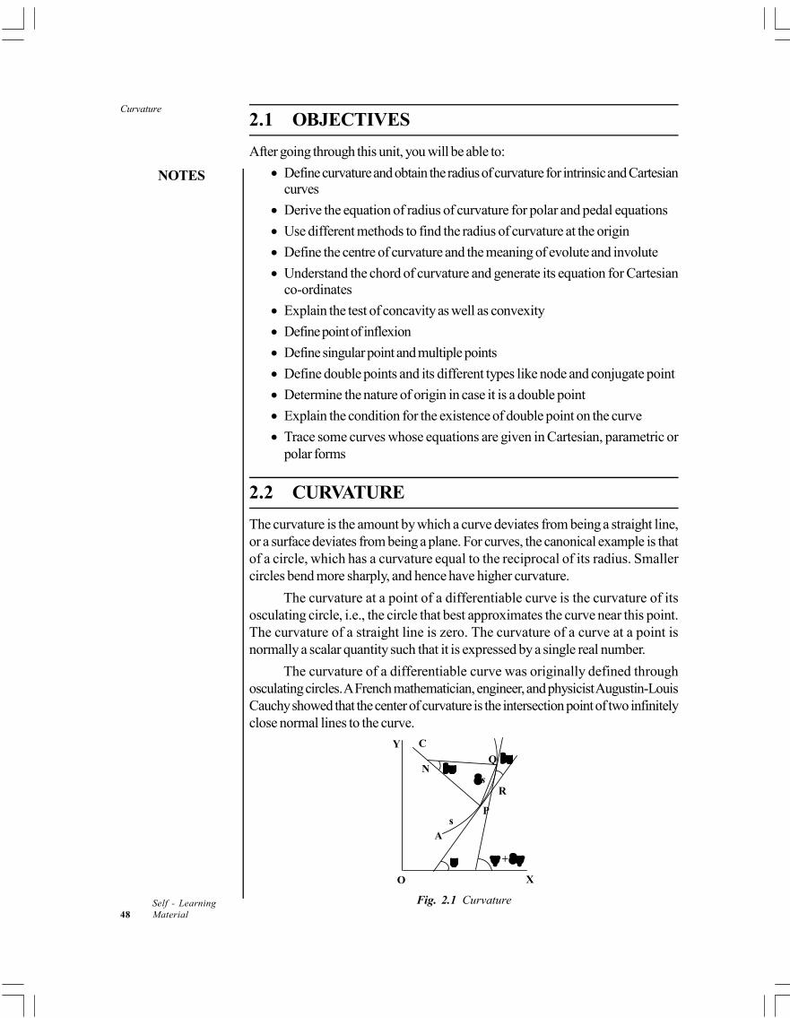
Curvature
NOTES
Self - Learning48 Material
2.1 OBJECTIVES
After going through this unit, you will be able to:
Define curvature and obtain the radius of curvature for intrinsic and Cartesiancurves
Derive the equation of radius of curvature for polar and pedal equations
Use different methods to find the radius of curvature at the origin
Define the centre of curvature and the meaning of evolute and involute
Understand the chord of curvature and generate its equation for Cartesianco-ordinates
Explain the test of concavity as well as convexity
Define point of inflexion
Define singular point and multiple points
Define double points and its different types like node and conjugate point
Determine the nature of origin in case it is a double point
Explain the condition for the existence of double point on the curve
Trace some curves whose equations are given in Cartesian, parametric orpolar forms
2.2 CURVATURE
The curvature is the amount by which a curve deviates from being a straight line,or a surface deviates from being a plane. For curves, the canonical example is thatof a circle, which has a curvature equal to the reciprocal of its radius. Smallercircles bend more sharply, and hence have higher curvature.
The curvature at a point of a differentiable curve is the curvature of itsosculating circle, i.e., the circle that best approximates the curve near this point.The curvature of a straight line is zero. The curvature of a curve at a point isnormally a scalar quantity such that it is expressed by a single real number.
The curvature of a differentiable curve was originally defined throughosculating circles. A French mathematician, engineer, and physicist Augustin-LouisCauchy showed that the center of curvature is the intersection point of two infinitelyclose normal lines to the curve.
X O
Y
P
R
Q N
C
A s
+
s
Fig. 2.1 Curvature
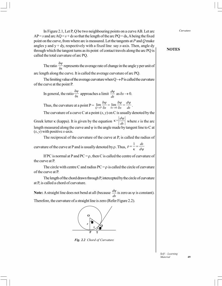
NOTES
Curvature
Self - LearningMaterial 49
In Figure 2.1, Let P, Q be two neighbouring points on a curve AB. Let arcAP = s and arc AQ = s + ds so that the length of the arc PQ = ds, A being the fixedpoint on the curve, from where arc is measured. Let the tangents at P and Q makeangles y and y + dy, respectively with a fixed line say x-axis. Then, angle dythrough which the tangent turns as its point of contact travels along the arc PQ iscalled the total curvature of arc PQ.
The ratio δψ
δsrepresents the average rate of change in the angle y per unit of
arc length along the curve. It is called the average curvature of arc PQ.
The limiting value of the average curvature when Q P is called the curvatureof the curve at the point P.
In general, the ratioδψ
δs approaches a limit
ψd
ds as s 0.
Thus, the curvature at a point P = 0
lim limQ P s
d
s s ds
.
The curvature of a curve C at a point (x, y) on C is usually denoted by the
Greek letter (kappa). It is given by the equation κ =d
ds
where s is the arc
length measured along the curve and is the angle made by tangent line to C at(x, y) with positive x-axis.
The reciprocal of the curvature of the curve at P, is called the radius of
curvature of the curve at P and is usually denoted by . Thus, 1
ρκ
ds
d
If PC is normal at P and PC = , then C is called the centre of curvature ofthe curve at P.
The circle with centre C and radius PC = is called the circle of curvatureof the curve at P.
The length of the chord drawn through P, intercepted by the circle of curvatureat P, is called a chord of curvature.
Note: A straight line does not bend at all (because ψd
dsis zero as is constant).
Therefore, the curvature of a straight line is zero (Refer Figure 2.2).
P T
Q
O
r
s
Fig. 2.2 Chord of Curvature
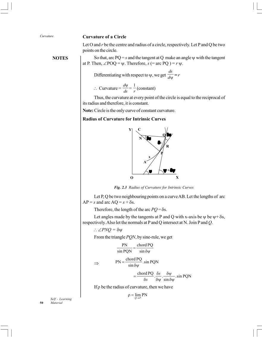
Curvature
NOTES
Self - Learning50 Material
Curvature of a Circle
Let O and r be the centre and radius of a circle, respectively. Let P and Q be twopoints on the circle.
So that, arc PQ = s and the tangent at Q make an angle with the tangentat P. Then, POQ = . Therefore, s (= arc PQ ) = r .
Differentiating with respect to , we get ds
d = r
Curvature = ψd
ds=
1
r(constant)
Thus, the curvature at every point of the circle is equal to the reciprocal ofits radius and therefore, it is constant.
Note: Circle is the only curve of constant curvature.
Radius of Curvature for Intrinsic Curves
X O
Y
P
R
Q N
C
A s
+
s
Fig. 2.3 Radius of Curvature for Intrinsic Curves
Let P, Q be two neighbouring points on a curve AB. Let the lengths of arcAP = s and arc AQ = s + s.
Therefore, the length of the arc PQ = s.
Let angles made by the tangents at P and Q with x-axis be be + s,respectively. Also let the normals at P and Q intersect at N. Join P and Q.
PNQ =
From the triangle PQN, by sine-rule, we get
chord PQPN
sin PQN sin
chord PQ
PN .sin PQNsin
chord PQ
. . .sin PQNsin
s
s
If be the radius of curvature, then we have
lim PNQ P
NOTES
Curvature
Self - LearningMaterial 51
0
chord PQlim . . .sin PQN
sins
s
s
[ s 0, 0, 0
chord PQlim 1s s
, PQN
2
and 1
sin
]
ds
d
The angle between the tangents to the curve at P and Q, i.e., is calledthe angle of contingence of the arc PQ. The relation between s and for a curveis called its intrinsic equation.
Thus, we can say that at a point P
arc PQlim
Angle of Contigence of arc PQQ P.
2.2.1 Radius of Curvature for Cartesian Curves
Analytical measure of the radius of curvature in Cartesian co-ordinates include thegeneral conic, cissoid and conchoid.
Radius of Curvature for Explicit Equation y = f(x)
Equation of the curve is y = f(x).
Let be the angle which the tangent at any point P(x, y) on the curvemakes with the x-axis.
Then sin , cos tandy dydx
ds ds dx ...(1)
Differentiating both sides with respect to x, we get,
2
22
(sec )d y d
dx dx
2(1 tan ) .
d ds
ds dx
2
1 .dy d ds
dx ds dx
[using Equation (1)]
But 1d
dx
121 2
2 2and = sec (1 tan ) = 1+dyds
dx dx
Using these,
12 22 2
2
11 1
d y dy dy
dx dx dx
Hence,
32 2
2
2
1dy
dx
d y
dx
The above formula can also be written as
32 2
1
2
1 y
y
Curvature
NOTES
Self - Learning52 Material
Note: This formula is not appropriate when the tangent is parallel to y-axis,
i.e., when dy
dx is infinite.
Since, the value of radius of curvature depends only on the curve and noton the axes, therefore in such cases we can interchange the axes of x and y and
we get
32 2
2
2
1dx
dy
d xdy
Radius of Curvature for Parametric Equations x = f(t), y = (t)
The equations of curve are given by x = f(t), y = (t),
Then /dy dy dx
dx dt dt , i.e.,
'
'
dy y
dx x
where xand y denotes the differential coefficients of x and y with respect to t,respectively.
Also,2
2
'
'
d y d y
dx dx x
'
.'
d y dt
dt x dx 2
' '' ' '' 1.
' '
x y y x
x x
1dt
dx x
3
' '' ' ''
'
x y y x
x
Putting the values of dy
dx and
2
2
d y
dx in the equation
32 2
2
2
1dy
dx
d y
dx
,we get
32 2
3
'1
'
' '' ' ''
'
y
x
x y y x
x
2 2 3/ 2( ' ' )
' '' ' ''
x y
x y y x
Radius of Curvature for Implicit Equation f(x, y) = 0
Equation of the curve is f(x) = 0
At a point where, fy 0, we get
x
y
fdy
dx f
and
2 22
2 3
2xx x y xy yy xy
y
f f f f f f fd y
dx f
NOTES
Curvature
Self - LearningMaterial 53
Since,
32 2
2
2
1dy
dx
d y
dx
32 2
3
2 2
1 .
2
xy
y
xx y x y xy yy x
ff
f
f f f f f f f
32 2 2
2 22
x y
xx y x y xy yy x
f f
f f f f f f f
Radius of Curvature when x and y are Function of s
We know that, cosdx
ds … (2)
and sindy
ds … (3)
By differentiating Equation (2) with respect to s, we get
2
2sin
d d x
ds ds
… (4)
2
2
1.
dy d x
ds ds
2
2
dy
dsd x
ds
Now, differentiating Equation (3) with respect to s, we have2
2cos
d d y
ds ds
… (5)
2
2
1.
dx d y
ds ds
2
2
dx
dsd y
ds
By squaring and adding Equations (4) and (5), we get2 22 2 2
2 2
d d x d y
ds ds ds
2 22 2
2 2 2
1 d x d y
ds ds
….(6)
Again,1
sin .dy dy d dy
ds d ds d
….(7)
And1
cos .dx dx d dx
ds d ds d
….(8)
By squaring and adding Equation (7) and (8), we get2 2
2 dx dy
d d
Example 2.1: Prove that for the curve 3 3cos , sinx a y a or the curve
2 / 3 2 / 3 2 / 3x y a at 3cos , sin3 ; 3 sin cosa a a .
Curvature
NOTES
Self - Learning54 Material
Solution: The equation of the curve is 3 3cos , sinx a y a …(i)
2' 3 cos .sindx
x ad
2' 3 sin .cosdx
y ad
Also, 2 2'' 3 cos 2sin cos ,x a
2 2'' 3 sin 2cos sin ,y a
3/ 2'2 '2
' '' '' '
x y
x y x y
3/ 2 3/ 22 2 2 2 2
2 2 2 2 2 2 2
9 sin cos cos sin
9 sin cos 2cos sin 2sin cos
a
a
2 2 2 2 2 2 29 sin cos 2cos sin 2sin cosa 3 sin cosa (numerically)
Example 2.2: If 1 2, be radii of curvature at the extremities of a pair of semi-conjugate diameters of an ellipse, prove that
2 / 3 2 / 3 2 / 3 2 21 2 .ab a b
Solution: Let the ellipse be 2 2
2 21
x y
a b
Its parametric equations are cos ,x a siny b
' sin , ' cosx a y b ; cos , sinx a y b
3/ 22 2 2 2
3 32 2
sin coscos , sin
sin cos
a ba b
ab ab
3/ 22 2 2 2sin cosa b
ab
… (i)
Let CP and CD be two semi-conjugate diameters. If the co-ordinates of P
are cos , sina b , then co-ordinates of D are cos , sin2 2
a b
If 1 is the radius of curvature at P, then
3/ 22 2 2 2
1
sin cosa b
ab
Changing ,2
we get
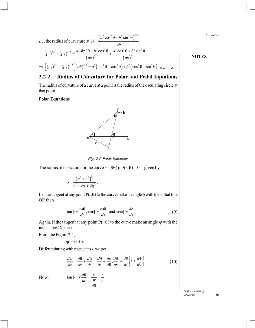
NOTES
Curvature
Self - LearningMaterial 55
2 , the radius of curvature at 3/ 22 2 2 2cos sina b
Dab
2 2 2 2 2 2 2 22 / 3 2 / 3
1 2 2 /3 2 / 3
sin cos cos sina b a b
ab ab
2 / 3 2 / 3 2 / 3 2 2 2 2 2 21 2 sin cos cos sinab a b 2 2a b
2.2.2 Radius of Curvature for Polar and Pedal Equations
The radius of curvature of a curve at a point is the radius of the osculating circle atthat point.
Polar Equations
X O
T
P(r, )
r
L
p
Figure 4.5
Fig. 2.4 Polar Equations
The radius of curvature for the curve r = f() or f(r, ) = 0 is given by
3
2 2 21
2 22 12
r r
r rr r
.
Let the tangent at any point P(r,) to the curve make an angle with the initial lineOP, then
θ θtan , sin and cos
rd rd dr
dr ds ds , … (9)
Again, if the tangent at any point P(r,) to the curve make an angle with theinitial line OX, then
From the Figure 2.4,
= +
Differentiating with respect to s, we get
d d d
ds ds ds
.
d d d
ds d ds
1
d d
ds d
… (10)
Now,1
tand r r
rdrdr rd
Curvature
NOTES
Self - Learning56 Material
Again differentiating with respect to , we get
22 1 1 2 1 2
2 21 1
sec .r r rr r rrd
d r r
2 2 2
1 2 1 2 1 22 2 2 2 2
1 1 21 2
1
sec (1 tan1
r rr r rr r rrd
d r r rr
r
1
tanr
r
21 2
2 21
r rr
r r
… (11)
Also,1
sincosec
dr
ds
2 2 21
1 1 1.
1 cot
d
ds r r r
… (12)
From Equations (10), (11) and (12), we get
2 2 21 2 2 1
2 2 32 22 21 21
1
211
r rr r rr rd
ds r rr r r r
32 2 2
1
2 22 12
r rds
d r rr r
Where 2
1 2anddr d r
r rd d
Corollary: If the equation of the curve is in the form u = f() where 1
ur
, then
2 2 3/ 21
32
( )ρ=
( )
u u
u u u
.
Proof: Given,1
ur
1
ru
Differentiating it with respect to , we get
11 2 2
1
θ
udur
du u , where 1 θ
duu
d
and2 2
2 1 1 1 22 4 3
.2 2u u u uu u uur
u u
, where
2
2 2θ
d uu
d
32 21
2 42 2 3/ 21
2 2 2 22 1 1 2 1
2 4 4
1
( )ρ =
2 2 21
u
u ur r
r rr r u uu u
u u u
2 2 3/ 2
13
2
( )ρ=
( )
u u
u u u
NOTES
Curvature
Self - LearningMaterial 57
Radius of Curvature for Pedal Equations
Theorem 2.1: If be the radius of curvature for the curve
p = f(r), thendr
rdp
.
Proof: Let the tangent at any point to the curve make an angle with the initialline OX.
Then, = +
d d d
ds ds ds
... (13)
Also, p = r sin …(14)
Differentiating Equation (14) with respect to r, we get
cos . sindp d
rdr dr
. .dr d d
r rds dr ds
sin ,cosd dr
rds ds
d d
rds ds
dr
ds
[Using Equation (13)]
1
.dp
rdr
drr
dp
Rules to Transform Polar Equation to Pedal Equation
1. Use the relation tand
rdr
and find .
2. Put this value of in sinp r
3. Eliminate to get the equation in Pedal form.
Example 2.3: Find the radius of curvature for the parabola 2
1 cos .a
r and
show that the square of the radius of curvature varies as the cube of the focaldistance.
Solution: Given, the equation of parabola is 2
1 cosa
r …(i)
Putting 1
ur
in (i), we get 2 1 cosau …(ii)
Differentiating (ii) with respect to we have 12 sinau …(iii)
Curvature
NOTES
Self - Learning58 Material
Differentiating (iii) with respect to , we have 22 cosau
3/ 22 21
3 22
u u
u u u
3/ 22 2
2
3
1 cos sin
2 4
1 cos 1 cos cos
2 2 2
a a
a a
3 / 2
33 / 2
3 / 23
4
12 1 cos
4 2 281 1 cos1 cos
16
aa ra
a
2 34r
a
In the given equation of the parabola, i.e., 2
1 cosa
r , the pole is at the
focus. Therefore, the focal distance of the point on the parabola is r. Hence, thesquare of the radius of curvature varies as the cube of the focal distance.
Example 2.4: Find the radius of curvature for the curve cos .n nr a n
Solution: The equation of the curve is cos .n nr a n …(i)
log log logcosn r n a n
Differentiating, 1. sin
cos
n drn n
r d n
cot
dr n
dr
Also, tan cotd
r ndr
tan tan2
n
2n
…(ii)
Now, sin sin2
p r r n
cos .
n
n
rr n r
a
Pedal equation of the given curve is 1n
n
rp
a
…(iii)
1.
1 1
n n
n n
dr a ar r
dp n r n r
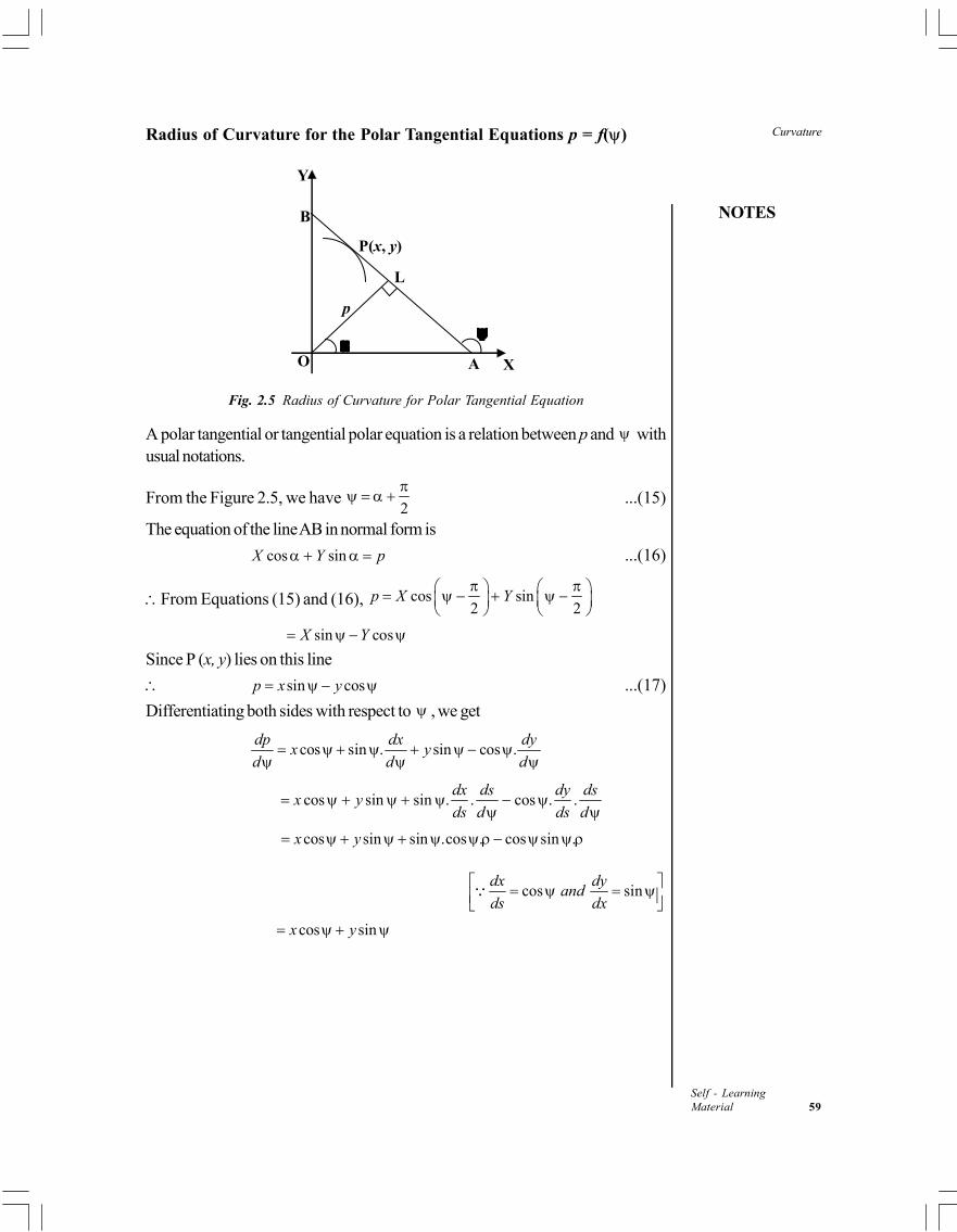
NOTES
Curvature
Self - LearningMaterial 59
Radius of Curvature for the Polar Tangential Equations p = f()
Y
A
O X
L
P(x, y)
B
p
Figure 4.6 Fig. 2.5 Radius of Curvature for Polar Tangential Equation
A polar tangential or tangential polar equation is a relation between p and withusual notations.
From the Figure 2.5, we have 2
...(15)
The equation of the line AB in normal form is
cos sinX Y p ...(16)
From Equations (15) and (16), cos sin2 2
p X Y
sin cosX Y
Since P (x, y) lies on this line
sin cosp x y ...(17)
Differentiating both sides with respect to , we get
cos sin . sin cos .dp dx dy
x yd d d
cos sin sin . . cos . .dydx ds ds
x yds d ds d
cos sin sin .cos . cos sin .x y
cos sindx dy
andds dx
cos sinx y
Curvature
NOTES
Self - Learning60 Material
Again differentiating with respect to , we have2
2sin cos . cos sin
d p dx dyx y
d d d
sin cos cos . sin . .dx ds dy ds
x yds d ds d
2 2cos . sin .p p
2
2
d pp
d
Example 2.5: If be the angle which the radius vector of the curve r = f()
makes with the tangent, prove that sin 1ρ θ
r d
d
, where is the radius of
curvature. Apply this result to show that
2
a for the circle r = a cos .
Solution: We know that = + Differentiatng with respect to s
.d d d d d d
ds ds ds ds d ds
1
d d
ds d
1 sin
1ρ θ
d
r d
sind
rds
sin 1ρ θ
r d
d
… (i)
Now, equation of the circle is r = a cos
Differentiatng with respect to , we get
sindr
ad
tan = cos
cot tansin 2
d ar
dr a
12
d
d
From (i), sin 1ρ θ
r d
d
=
cosec
1θ
rdd
NOTES
Curvature
Self - LearningMaterial 61
cos .cosec
2cosθsecθ =
1+1 2 2
aa a
cos sec
2 2
a a
2.2.3 Radius of Curvature at the Origin
The following methods are used to find the radius of curvature at the origin.
Method of Direct Substitution
In this method, we put x = 0 and y = 0 directly in the the formula,
32 2
1
2
1 y
y
.
We can also find first the values of dy
dx and
2
2
d y
dx at (0, 0) and then substitute
these values in this formula.
Method of Expansion
When the x-axis or the y-axis is not the tangent at the origin, we use the method ofexpansion.
Let the equation of the curve be y = f(x)
Since it passes through the origin (0, 0)
f(0) = 0.
By Maclaurin’s Expansion, we have
2 3
(0) '(0) ''(0) '''(0) ...2
x xy f xf f f
2 3
'(0) ''(0) '''(0) ...2
x xy xf f f
…. (18)
If the equation of the curve is such that y can be expanded in powers of x bytrignometrical or algebraic methods, then we have
2 31 1...
2y px qx rx
…. (19)
On comparing Equations (18) and (19), we get
p = (0)f = (y1)
0 ; q = (0)f = (y
2)
0, etc.
Now differentiating Equation (19) with respect to x, 21
1...
2y p qx rx
Differentiating again 2 ...y q rx At the origin, y
1 = p and y
2 = q
i.e., (y1)
0 = p and (y
2)
0 = q
at the origin
3 3
2 2 2 21 0
2 0
1 1y p
y q
Curvature
NOTES
Self - Learning62 Material
Newton’s Method
Theorem 2.2: If the curve passes through the origin and axis of x is the tangent atthe origin, then
(at the origin) =
2
00
lim2x
y
x
y
Proof: Since, x-axis is the tangent at the origin, then
f(0) = 0, (0)f = 0 and (0)f = (0,0)
dy
dx
Hence, by Maclaurin’s expansion,2 3
(0) '(0) ''(0) '''(0) ...2
x xy f xf f f
2 3
0 0 ...,above2 3
x xx q r
2 3
...2
x xq r
2
2...termsof
y xq r x
x r
At the origin x 0, y 0 so that 200
2limxy
yq
x
Hence
32 2
1
2 2
1 1y
y y
1 0y
1
q
2
00
lim2x
y
x
y
Note: Similarly, if the curve passes through the origin and y-axis is the tangent atthe origin, then the radius of curvature at the origin is given by
2
00
lim2x
y
y
x
.
Curvature at the Origin when Polar Equation of the Curve is Given
If the initial line, i.e., 0 is a tangent to the curve r f , then
(at the pole)
2 2 2
0 00 0
coslim lim
2 2 sinxy r
x r
y r
(Changing to polar co-ordinates)
NOTES
Curvature
Self - LearningMaterial 63
2
0 00 0
lim . .cos lim2 sin 2
r r
r r
0lim 1
sin
By L’ Hospital’s rule,
00
1lim
2r
dr
d
Corollary: Tangents at the origin.
Let the equation of the curve which passes through the origin be
2 21 1 1 .... 0ax by a x b xy c y …(20)
Let 2 3
....2! 3!
x xy px q r be its Maclaurin’s expansion.
Putting this value of y in Equation (20), we get22 2
21 1... .... ... 0,
2! 2!
x xax b px q a x b x px q
an identity..
Equating the co-efficients of x on both sides, we get
0 , 0a
a bp p bb
Since, ,a
pb
where ' 0p f is the slope of the tangent at the origin,
thus the equation of the tangent at the origin is
0 0a
y xb
0ax by
which are the lowest degree terms of the equation of the curve equated to zero.
Similarly, if the terms of the first degree in x and y are wanting in theequation of the curve, then the tangents at the origin are given
by 2 21 1 1 0a x b xy c y which are again the lowest degree terms of the equation
equated to zero and so on.
Note: Newton’s method for finding the radius of curvature shall be applied onlywhen either x-axis, i.e., 0y or y-axis, i.e., 0x is a tangent to the curve at theorigin.
Example 2.6: Find the radius of curvature at the origin for the curve
4 3 2 3 2 22 4 6 3 2 4 0x x y xy y x xy y x .
Solution: Since, the equation does not contain any constant term, therefore, thecurve passes through the origin, and the tangent at the origin is 0x ,
i.e., y-axis is a tangent at the origin. Thus, by Newton’s method,
(at the origin) =
2
00
lim2x
y
y
x
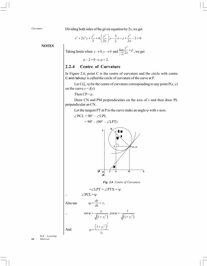
Curvature
NOTES
Self - Learning64 Material
Dividing both sides of the given equation by 2x, we get
2 2 23 2 3
2 6. . 2 02 2 2 2
y y yx x y y x y
x x
Taking limits when 0, 0x y and
2
00
lim2x
y
y
x
, we get
2 0 2 .
2.2.4 Centre of Curvature
In Figure 2.6, point C is the centre of curvature and the circle with centreC and radius is called the circle of curvature of the curve at P.
Let C(, ) be the centre of curvature corresponding to any point P(x, y)on the curve y = f(x).
Then CP = .
Draw CN and PM perpendiculars on the axis of x and then draw PLperpendicular on CN.
Let the tangent PT at P to the curve make an angle with x-axis.
PCL = 90 – CPL
= 90 – (90 – LPT)
X O
Y
P (x, y)
N
L
C
M
T X
Y
(, ) D
Figure 4.7
Fig. 2.6 Centre of Curvature
=LPT = PTX = PCL=
Also tan = 1
dyy
dx
1
2 21 1
1sin ,cos
1 1
y
y y
And
32 2
1
2
1 y
y
NOTES
Curvature
Self - LearningMaterial 65
Now, = ON = OM – NM = OM – PL = x – CP sin = x – sin [from LPC]
=
32 2
1 11
22 21
1.
1
y yx
yy
…(21)
= CN = CL +LN = CL + PM
= y + CP cos = y + cos =
32 2
1
122 2
1
1 1.
1
yy
yy
or 21
2
11y y
y …(22)
Corollary 1: Putting ρ ,sin ψ ,cosψψ
ds dy dx
d ds ds , we get
ξ .ds dy dy
x xd ds d
and .
ds dx dxy y
d ds d
Corollary 2: The equation of the circle of curvature at a given point of the curve.
Let be the radius of curvature and (, ) the centre of curvature at the givenpoint. Then, the equation of the circle of curvature is given by(x – )2 + (y – )2 = 2.
Evolute and Involute
The locus of the centre of curvature of the given curve is called the evolute of thecurve and the curve itself is called the involute of its evolute.
Example 2.7: Find the coordinates of the centre of curvature at any point(x, y) of a parabola y2 = 4ax. Also find the equation of the evolute of the parabola.
Solution: Equations of the parabola is y2 = 4ax
1 12
2 4 ora
yy a yy
and2
2 12 3
2 4.
a ay y
y y
If (, ) is the centre of curvature, then
2
221
1 22
3
41
ξ 14
a a
y yyx y x
ayy
[ y2 = 4ax]
= 3x + 2a … (i)
And
2
22
1 22
3
41
1η 1
4
a
yy y y
ayy
3 / 22x
a … (ii)
The centre of curvature at (x, y) is 3 / 22
3 2 ,x
x aa
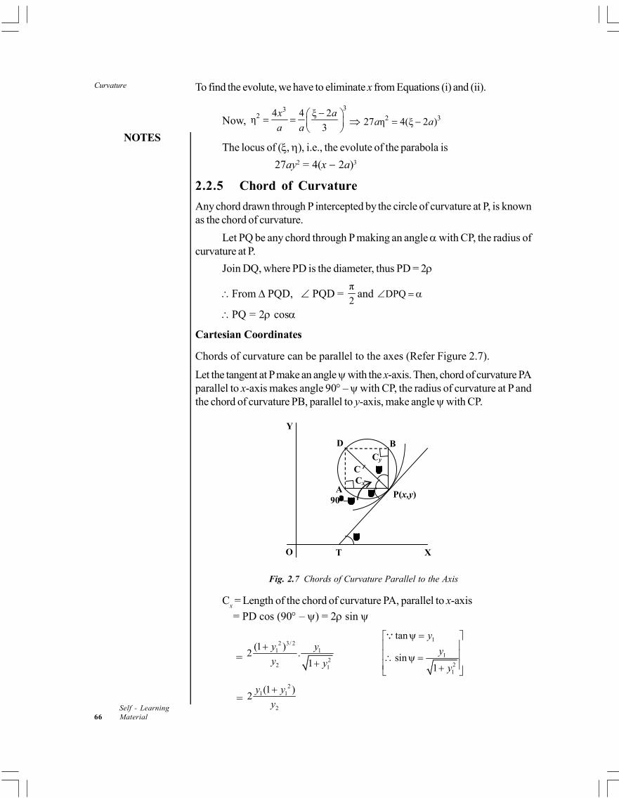
Curvature
NOTES
Self - Learning66 Material
To find the evolute, we have to eliminate x from Equations (i) and (ii).
Now, 33
2 4 4 ξ 2η
3
x a
a a
2 327 η 4(ξ 2 )a a
The locus of (, ), i.e., the evolute of the parabola is
27ay2 = 4(x 2a)3
2.2.5 Chord of Curvature
Any chord drawn through P intercepted by the circle of curvature at P, is knownas the chord of curvature.
Let PQ be any chord through P making an angle with CP, the radius ofcurvature at P.
Join DQ, where PD is the diameter, thus PD = 2
From PQD, PQD = π
2and DPQ
PQ = 2 cos
Cartesian Coordinates
Chords of curvature can be parallel to the axes (Refer Figure 2.7).
Let the tangent at P make an angle with the x-axis. Then, chord of curvature PAparallel to x-axis makes angle 90 – with CP, the radius of curvature at P andthe chord of curvature PB, parallel to y-axis, make angle with CP.
X T O
P(x,y) A
D
C
90–
Cy
Cx
B
Y
Fig. 2.7 Chords of Curvature Parallel to the Axis
Cx = Length of the chord of curvature PA, parallel to x-axis
= PD cos (90 – ) = 2 sin
=
2 3/ 21 1
22 1
(1 )2 .
1
y y
y y
1
1
21
tan
sin1
y
y
y
= 2
1 1
2
(1 )2
y y
y
NOTES
Curvature
Self - LearningMaterial 67
Cy = Length of the chord of curvature PB, parallel to y-axis
= PD cos = 2 cos
=
2 3/ 21
22 1
(1 ) 12 .
1
y
y y
=2
1
2
(1 )2
y
y
Hence, chord PA (parallel to x-axis) = 2 sin =2
1 1
2
(1 )2
y y
y
and chord PB (parallel to y-axis) = 2 cos =2
1
2
(1 )2
y
y
Example 2.8: If Cx and C
y be the chords of curvature parallel to the axis of x and
y respectively at any point of the curve y = aex/a, prove that 2 2
1 1 1
2x y xC C aC .
Solution: Equation of the curve is y = aex/a
/1 2 1 2
1 1. , .x a yy
y ae y ya a a a
tan = y1
sin = 1
2 21
y
a y
cos = 2 2
1
a
a y
Cx = 2 sin =
32
1 11
2 221
2. 1
1
y y
y y
3 221
2
1P
y
y
211
2
2. 1y
yy
2 2
22. 1
y a y
a y a
2 2
22
a ya
a
2 22 a y
a
Cy = 2 cosψ
32 2
1
12 22
1
1 12.
1
y
yy
2
1
2
2. 1 y
y
2
2 22
2
2. 12.
ya ya
y ya
2 2 2 2
2 2 2 2 2 2 2 2 2 2 2
1 1
4( ) 4( ) 4( )x y
a y a y
C C a y a y a y
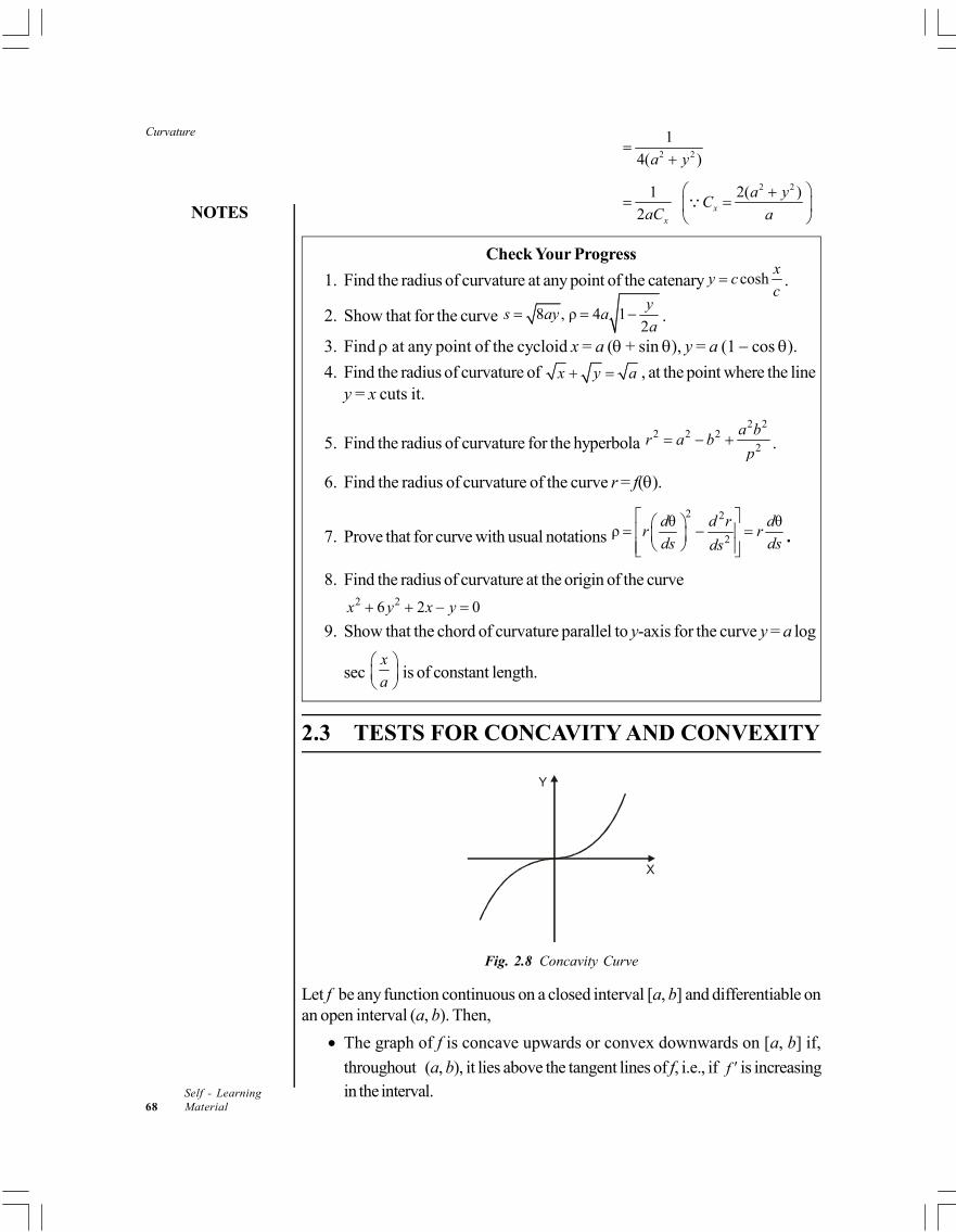
Curvature
NOTES
Self - Learning68 Material
2 2
1
4( )a y
1
2 xaC
2 22( )x
a yC
a
Check Your Progress
1. Find the radius of curvature at any point of the catenary coshx
y cc
.
2. Show that for the curve 8 , ρ 4 12
ys ay a
a .
3. Find at any point of the cycloid x = a ( + sin ), y = a (1 cos ).
4. Find the radius of curvature of x y a , at the point where the liney = x cuts it.
5. Find the radius of curvature for the hyperbola 2 2
2 2 22
a br a b
p .
6. Find the radius of curvature of the curve r = f().
7. Prove that for curve with usual notations
2 2
2
θ θρ
d d r dr r
ds dsds
.
8. Find the radius of curvature at the origin of the curve2 26 2 0x y x y
9. Show that the chord of curvature parallel to y-axis for the curve y = a log
sec x
a
is of constant length.
2.3 TESTS FOR CONCAVITY AND CONVEXITY
X
Y
Fig. 2.8 Concavity Curve
Let f be any function continuous on a closed interval [a, b] and differentiable onan open interval (a, b). Then,
The graph of f is concave upwards or convex downwards on [a, b] if,
throughout (a, b), it lies above the tangent lines of f, i.e., if f is increasingin the interval.
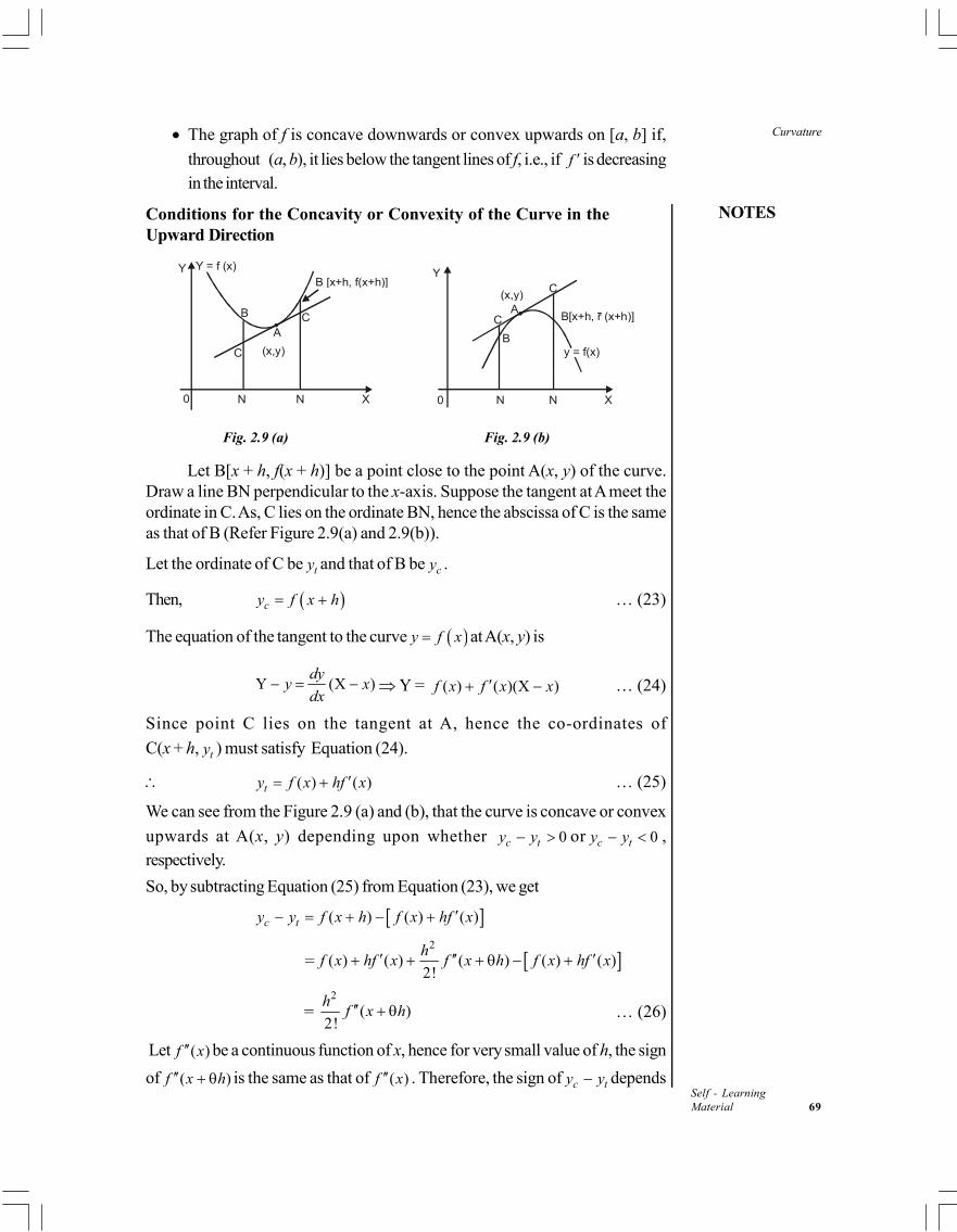
NOTES
Curvature
Self - LearningMaterial 69
The graph of f is concave downwards or convex upwards on [a, b] if,
throughout (a, b), it lies below the tangent lines of f, i.e., if f is decreasingin the interval.
Conditions for the Concavity or Convexity of the Curve in theUpward Direction
Y Y = f (x)
A
B C
(x,y)
0 XN
B [x+h, f(x+h)]
N
C
Y
(x,y)A
B
C
0 N X
B[x+h, r (x+h)]
C
N
y = f(x)
Fig. 2.9 (a) Fig. 2.9 (b)
Let B[x + h, f(x + h)] be a point close to the point A(x, y) of the curve.Draw a line BN perpendicular to the x-axis. Suppose the tangent at A meet theordinate in C. As, C lies on the ordinate BN, hence the abscissa of C is the sameas that of B (Refer Figure 2.9(a) and 2.9(b)).
Let the ordinate of C be ty and that of B be cy .
Then, cy f x h … (23)
The equation of the tangent to the curve y f x at A(x, y) is
Y (X )dy
y xdx
Y = ( ) ( )(X )f x f x x … (24)
Since point C lies on the tangent at A, hence the co-ordinates of
C(x + h, ty ) must satisfy Equation (24).
( ) ( )ty f x hf x … (25)
We can see from the Figure 2.9 (a) and (b), that the curve is concave or convex
upwards at A(x, y) depending upon whether 0c ty y or 0c ty y ,respectively.
So, by subtracting Equation (25) from Equation (23), we get
( ) ( ) ( )c ty y f x h f x hf x
= 2
( ) ( ) ( ) ( ) ( )2!
hf x hf x f x h f x hf x
= 2
( )2!
hf x h … (26)
Let ( )f x be a continuous function of x, hence for very small value of h, the sign
of ( )f x h is the same as that of ( )f x . Therefore, the sign of c ty y depends
Curvature
NOTES
Self - Learning70 Material
upon ( )f x because2
2!
his always positive. Thus, the curve is concave or convex
in upwards direction depending upon whether c ty y > 0 or
c ty y < 0, i.e., 2
20
d y
dx or
2
20
d y
dx .
Similarly, the curve is concave or convex in the positive direction of x-axis dependingupon whether
2
20
d x
dy or
2
20
d x
dy .
Note: The above proof can also be generalized for ( )nf x . In this case, the curve
is concave or convex in the upward direction depending upon whether
( ) 0nf x or ( ) 0nf x , n being even.
2.4 POINTS OF INFLECTION
A point of inflexion is a point on a curve at which the curve changes from beingconcave upwards to concave downwards or vice-versa.
If P(x, y) is a point of inflexion on the curve, then on one side of P, the curveis concave and on the other side it is convex. At the point of inflexion, the tangentcrosses the curve at that point.
Test for Point of Inflexion
If , ( )c f c is a point of inflexion on the graph of f, then either ( ) 0f c or f does
not exist at c. The converse may not necessarily be true.
Thus, a point is said to be a point of inflexion, if 2
20
d y
dx at this point and
2
2
d y
dxchanges sign while passing through this point, i.e.,
3
30
d y
dx at this point.
Steps for finding point of inflexion
(i) Find all the numbers at which ( ) 0f x
(ii) Use the test of concavity
(iii) There is an inflexion point, if the concavity changes; otherwise, there is noinflexion point.
NOTES
Curvature
Self - LearningMaterial 71
Example 2.9: Find the points of inflexion of the curve 6 5( 2) ( 3) .y x x
Solution: The given curve is 6 52 3 .y x x ...(i)
6 4 5 52 .5 3 6 2 3
dyx x x x
dx
5 42 3 5 2 6 3x x x x 5 4
2 3 11 28x x x
2
5 4 5 3 4 4
22 3 .11 2 11 28 .4 3 3 11 28 .5 2
d yx x x x x x x x
dx
= 4 32 3 11 2 3 4 2 11 28 5 3 ( 11 28x x x x x x x x
4 3 22 3 110 560 710x x x x
4 3 210 2 3 11 56 71x x x x
4 3 28 3 28 310 2 3
11 11x x x x
At the points of inflexion2
20
d y
dx
28 32,3, .
11x
At 2
22,
d yx
dx does not change sign as the corresponding factor 4
2x
remains +ve whether 2 or 2.x x
2x does not correspond to the point of inflexion.
Also, 2
2
d y
dx changes sign at 3x and
28 3
11x
.
Thus, these correspondences to the abscissa of the points of inflexion of thegiven curve.
Check Your Progress
10. Show that the curve y = log x is convex upwards everywhere.
11. Determine the point of inflexion on the curve
(2 sin ), (2 cos )x a y a
2.5 MULTIPLE POINTS
Singular point is a point on a curve at which the curve shows an extraordinary orunusual behaviour. Now, in this unit, we shall study about two particular types ofsingular points: multiple points and points of inflexion.
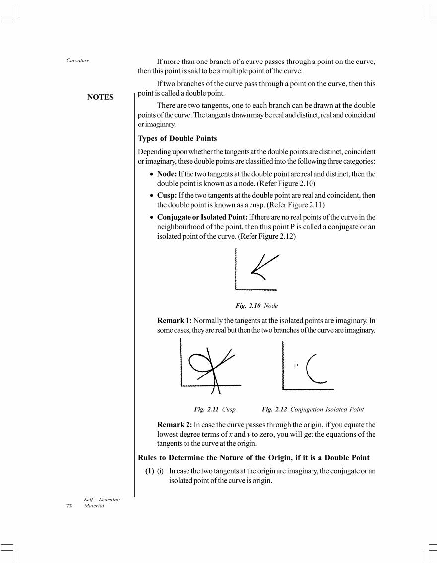
Curvature
NOTES
Self - Learning72 Material
If more than one branch of a curve passes through a point on the curve,then this point is said to be a multiple point of the curve.
If two branches of the curve pass through a point on the curve, then thispoint is called a double point.
There are two tangents, one to each branch can be drawn at the doublepoints of the curve. The tangents drawn may be real and distinct, real and coincidentor imaginary.
Types of Double Points
Depending upon whether the tangents at the double points are distinct, coincidentor imaginary, these double points are classified into the following three categories:
Node: If the two tangents at the double point are real and distinct, then thedouble point is known as a node. (Refer Figure 2.10)
Cusp: If the two tangents at the double point are real and coincident, thenthe double point is known as a cusp. (Refer Figure 2.11)
Conjugate or Isolated Point: If there are no real points of the curve in theneighbourhood of the point, then this point P is called a conjugate or anisolated point of the curve. (Refer Figure 2.12)
Fig. 2.10 Node
Remark 1: Normally the tangents at the isolated points are imaginary. Insome cases, they are real but then the two branches of the curve are imaginary.
P
Fig. 2.11 Cusp Fig. 2.12 Conjugation Isolated Point
Remark 2: In case the curve passes through the origin, if you equate thelowest degree terms of x and y to zero, you will get the equations of thetangents to the curve at the origin.
Rules to Determine the Nature of the Origin, if it is a Double Point
(1) (i) In case the two tangents at the origin are imaginary, the conjugate or anisolated point of the curve is origin.
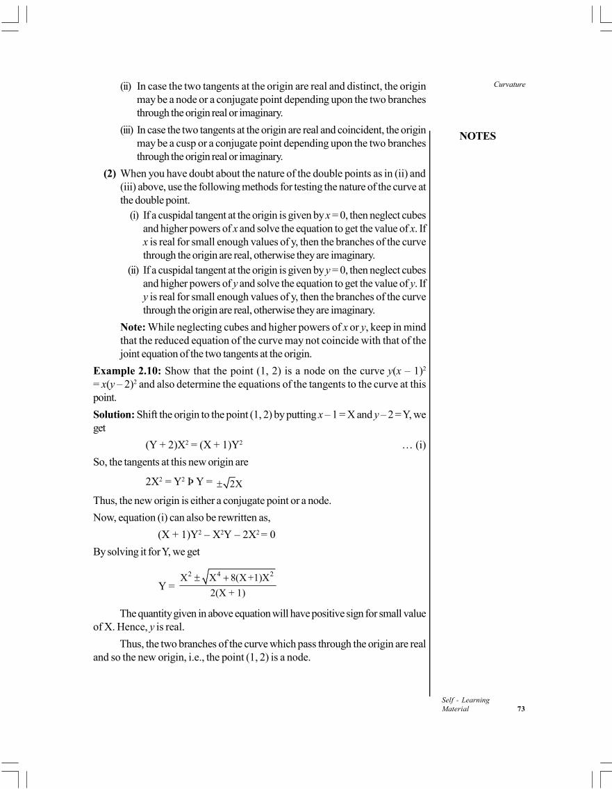
NOTES
Curvature
Self - LearningMaterial 73
(ii) In case the two tangents at the origin are real and distinct, the originmay be a node or a conjugate point depending upon the two branchesthrough the origin real or imaginary.
(iii) In case the two tangents at the origin are real and coincident, the originmay be a cusp or a conjugate point depending upon the two branchesthrough the origin real or imaginary.
(2) When you have doubt about the nature of the double points as in (ii) and(iii) above, use the following methods for testing the nature of the curve atthe double point.
(i) If a cuspidal tangent at the origin is given by x = 0, then neglect cubesand higher powers of x and solve the equation to get the value of x. Ifx is real for small enough values of y, then the branches of the curvethrough the origin are real, otherwise they are imaginary.
(ii) If a cuspidal tangent at the origin is given by y = 0, then neglect cubesand higher powers of y and solve the equation to get the value of y. Ify is real for small enough values of y, then the branches of the curvethrough the origin are real, otherwise they are imaginary.
Note: While neglecting cubes and higher powers of x or y, keep in mindthat the reduced equation of the curve may not coincide with that of thejoint equation of the two tangents at the origin.
Example 2.10: Show that the point (1, 2) is a node on the curve y(x – 1)2
= x(y – 2)2 and also determine the equations of the tangents to the curve at thispoint.
Solution: Shift the origin to the point (1, 2) by putting x – 1 = X and y – 2 = Y, weget
(Y + 2)X2 = (X + 1)Y2 … (i)
So, the tangents at this new origin are
2X2 = Y2 Þ Y = 2X
Thus, the new origin is either a conjugate point or a node.
Now, equation (i) can also be rewritten as,
(X + 1)Y2 – X2Y – 2X2 = 0
By solving it for Y, we get
Y = 2 4 2X X 8(X +1)X
2(X + 1)
The quantity given in above equation will have positive sign for small valueof X. Hence, y is real.
Thus, the two branches of the curve which pass through the origin are realand so the new origin, i.e., the point (1, 2) is a node.
Curvature
NOTES
Self - Learning74 Material
Now, the tangents at the new origin are
Y = 2X and Y = 2X
y – 2 = 2( 1)x and y – 2 = 2( 1)x
y = 2 2 2x and y = 2 2 2x
Condition for the Existence of a Double Point on a Curve
Suppose the equation of the curve is given by f (x, y) = 0 … (27)
By differentiating it with respect to x, we get 0f f dy
x y dx
… (28)
Equation (28) is a first degree equation in dy
dxand hence gives only one
value at any point P(x, y) on the curve. We know that there are two tangents to
the curve at double point. Hence, dy
dx should have two values which satisfy Equation
(28) But this is possible only if,
f
x
= 0 and f
y
= 0 … (29)
On solving Equation (29) for x and y simultaneously, we get the possibledouble points. As P(x, y) which lies on the curve f(x,y), therefore only those valueof x and y are to be considered as double point that satisfy Equation (27) also.
We now see the nature of the double point that is obtained from the above.
By differentiating Equation (28), x, we get 0f f dyd d
dx x dx y dx
2 2 2 2 2
2 2 20
f f dy f d y dy f f dy
y x dx y dx x y dxx dx y
Using f
y
= 0 from Equation (27) in the above equation, we get
22 2 2
2 22 0
f f dy f dy
x y dx dxx y
2 2f f
x y y x
22 2 2
2 22 0
f dy f dy f
dx x y dxy x
… (30)
Equation (30) is a quadratic equation in dy
dxand hence gives two values
dy
dx,
which provides the slopes of the tangents at the double point of the curve. Thesetangents may be real and distinct, real and coincident or imaginary dependingupon whether the discriminant (D) of Equation (30) is positive, zero or negative.

NOTES
Curvature
Self - LearningMaterial 75
i.e.,
22 2 2
2 2.
f f f
x y y x
>, = or < 0, respectively … (31)
Now, if(i) D > 0, double point is a node or a conjugate point(ii) D = 0, double point is a cusp or conjugate point(iii) D < 0, double point is a conjugate point.
Example 2.11: Find the position and nature of the double points on the curve2 2( 2) ( 1)y x x
Solution: Let 2 2, 2 1 0f x y x x y …(i)
Then 22 2 2 1
fx x x
x
and 2f
yy
For the double points 0f
x
and 0
f
y
2 2 2 2 0x x x
x = 2 and x = 4
3And y = 0
Thus, the possible double points are (2, 0) and4
,03
. But only (2, 0) satisfies
Equation (i). Therefore (2, 0) is the only double point.
Shifting the origin at (2, 0), Equation (i) transforms into
Y2 = X2(X + 1) …(ii)
The tangents at the new origin are Y2 = X2 i.e., Y = X
Thus the new origin is either a node or a conjugate point,
Solving Equation (ii) for Y, we get Y X X 1 which gives Y real forsmall values of X. Thus, the branches of the curve near the new origin are real.Therefore, the new origin or the point (2, 0) on Equation (i) is a node.
Check Your Progress
12. Find the nature of the origin for the curve 4 2 4 2 2( ).a y x x a
13. Find the position and nature of the double points of the curve
3 2 2 4 3 0x x y x y .
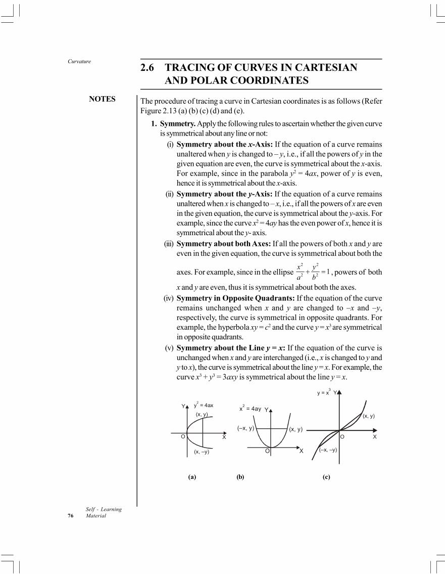
Curvature
NOTES
Self - Learning76 Material
2.6 TRACING OF CURVES IN CARTESIANAND POLAR COORDINATES
The procedure of tracing a curve in Cartesian coordinates is as follows (ReferFigure 2.13 (a) (b) (c) (d) and (e).
1. Symmetry. Apply the following rules to ascertain whether the given curveis symmetrical about any line or not:
(i) Symmetry about the x-Axis: If the equation of a curve remainsunaltered when y is changed to – y, i.e., if all the powers of y in thegiven equation are even, the curve is symmetrical about the x-axis.For example, since in the parabola y2 = 4ax, power of y is even,hence it is symmetrical about the x-axis.
(ii) Symmetry about the y-Axis: If the equation of a curve remainsunaltered when x is changed to – x, i.e., if all the powers of x are evenin the given equation, the curve is symmetrical about the y-axis. Forexample, since the curve x2 = 4ay has the even power of x, hence it issymmetrical about the y- axis.
(iii) Symmetry about both Axes: If all the powers of both x and y areeven in the given equation, the curve is symmetrical about both the
axes. For example, since in the ellipse 2 2
2 21
x y
a b , powers of both
x and y are even, thus it is symmetrical about both the axes.(iv) Symmetry in Opposite Quadrants: If the equation of the curve
remains unchanged when x and y are changed to –x and –y,respectively, the curve is symmetrical in opposite quadrants. Forexample, the hyperbola xy = c2 and the curve y = x3 are symmetricalin opposite quadrants.
(v) Symmetry about the Line y = x: If the equation of the curve isunchanged when x and y are interchanged (i.e., x is changed to y andy to x), the curve is symmetrical about the line y = x. For example, thecurve x3 + y3 = 3axy is symmetrical about the line y = x.
Y
O
(x, –y)
y = 4ax2
(x, y)
X
x = 4ay2
(–x, y) (x, y)
O X
Y
y = x3
Y
O X
(–x, y)–
(x, y)
(a) (b) (c)
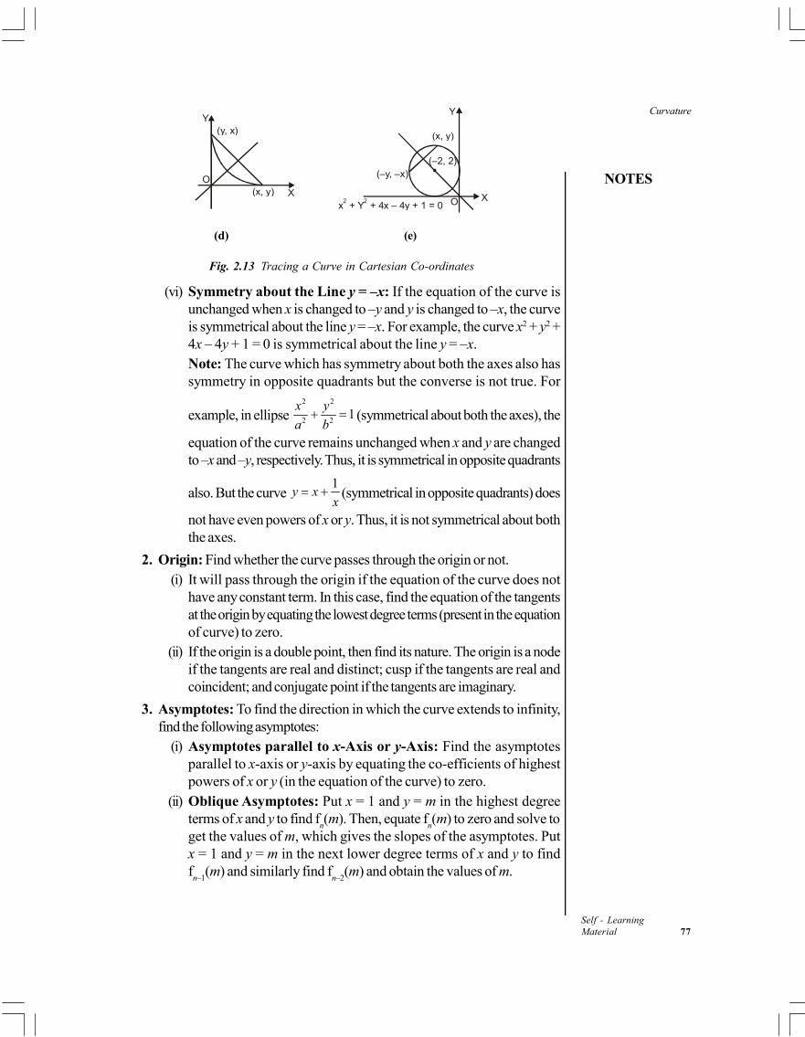
NOTES
Curvature
Self - LearningMaterial 77
Y
OX
(y, x)
(x, y)
Y
(x, y)
(–y, –x)(–2, 2)
XOx + Y + 4x – 4y + 1 = 02 2
(d) (e)
Fig. 2.13 Tracing a Curve in Cartesian Co-ordinates
(vi) Symmetry about the Line y = –x: If the equation of the curve isunchanged when x is changed to –y and y is changed to –x, the curveis symmetrical about the line y = –x. For example, the curve x2 + y2 +4x – 4y + 1 = 0 is symmetrical about the line y = –x.Note: The curve which has symmetry about both the axes also hassymmetry in opposite quadrants but the converse is not true. For
example, in ellipse 2 2
2 21
x y
a b (symmetrical about both the axes), the
equation of the curve remains unchanged when x and y are changedto –x and –y, respectively. Thus, it is symmetrical in opposite quadrants
also. But the curve 1
y xx
(symmetrical in opposite quadrants) does
not have even powers of x or y. Thus, it is not symmetrical about boththe axes.
2. Origin: Find whether the curve passes through the origin or not.(i) It will pass through the origin if the equation of the curve does not
have any constant term. In this case, find the equation of the tangentsat the origin by equating the lowest degree terms (present in the equationof curve) to zero.
(ii) If the origin is a double point, then find its nature. The origin is a nodeif the tangents are real and distinct; cusp if the tangents are real andcoincident; and conjugate point if the tangents are imaginary.
3. Asymptotes: To find the direction in which the curve extends to infinity,find the following asymptotes:
(i) Asymptotes parallel to x-Axis or y-Axis: Find the asymptotesparallel to x-axis or y-axis by equating the co-efficients of highestpowers of x or y (in the equation of the curve) to zero.
(ii) Oblique Asymptotes: Put x = 1 and y = m in the highest degreeterms of x and y to find f
n(m). Then, equate f
n(m) to zero and solve to
get the values of m, which gives the slopes of the asymptotes. Putx = 1 and y = m in the next lower degree terms of x and y to findf
n–1(m) and similarly find f
n–2(m) and obtain the values of m.
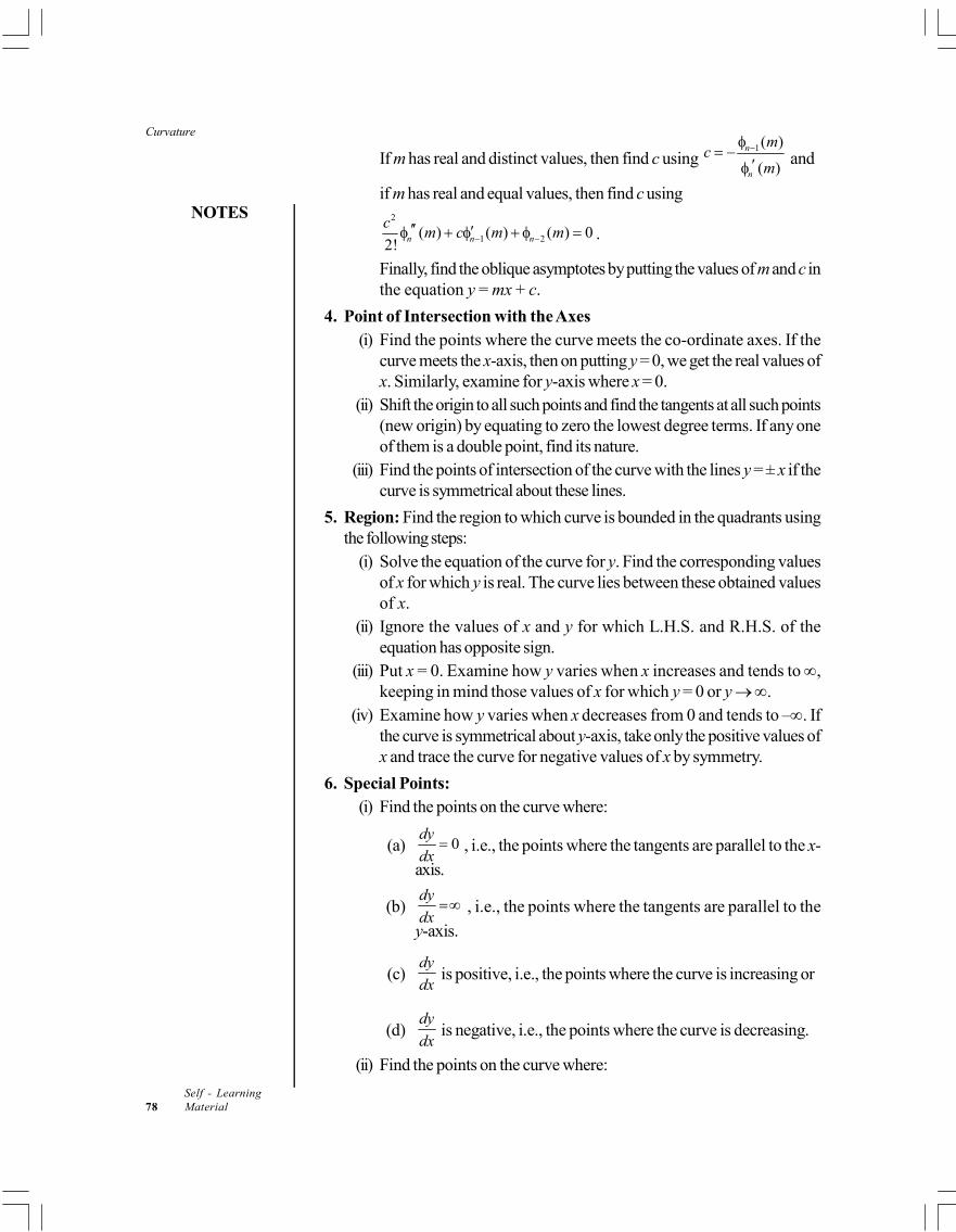
Curvature
NOTES
Self - Learning78 Material
If m has real and distinct values, then find c using 1( )
( )
n
n
mc
m
and
if m has real and equal values, then find c using2
1 2( ) ( ) ( ) 02! n n n
cm c m m
.
Finally, find the oblique asymptotes by putting the values of m and c inthe equation y = mx + c.
4. Point of Intersection with the Axes(i) Find the points where the curve meets the co-ordinate axes. If the
curve meets the x-axis, then on putting y = 0, we get the real values ofx. Similarly, examine for y-axis where x = 0.
(ii) Shift the origin to all such points and find the tangents at all such points(new origin) by equating to zero the lowest degree terms. If any oneof them is a double point, find its nature.
(iii) Find the points of intersection of the curve with the lines y = ± x if thecurve is symmetrical about these lines.
5. Region: Find the region to which curve is bounded in the quadrants usingthe following steps:
(i) Solve the equation of the curve for y. Find the corresponding valuesof x for which y is real. The curve lies between these obtained valuesof x.
(ii) Ignore the values of x and y for which L.H.S. and R.H.S. of theequation has opposite sign.
(iii) Put x = 0. Examine how y varies when x increases and tends to ,keeping in mind those values of x for which y = 0 or y .
(iv) Examine how y varies when x decreases from 0 and tends to –. Ifthe curve is symmetrical about y-axis, take only the positive values ofx and trace the curve for negative values of x by symmetry.
6. Special Points:(i) Find the points on the curve where:
(a) 0dy
dx , i.e., the points where the tangents are parallel to the x-
axis.
(b)dy
dx , i.e., the points where the tangents are parallel to the
y-axis.
(c)dy
dx is positive, i.e., the points where the curve is increasing or
(d)dy
dx is negative, i.e., the points where the curve is decreasing.
(ii) Find the points on the curve where:
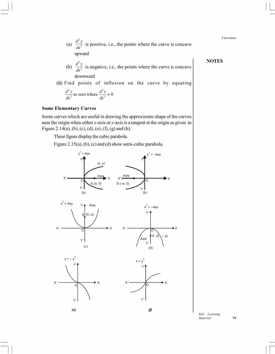
NOTES
Curvature
Self - LearningMaterial 79
(a)2
2
d y
dx is positive, i.e., the points where the curve is concave
upward
(b)2
2
d y
dx is negative, i.e., the points where the curve is concave
downward(iii) Find points of inflexion on the curve by equating
2 3
2 3to zero where 0
d y d x
dx dy
Some Elementary Curves
Some curves which are useful in drawing the approximate shape of the curvesnear the origin when either x-axis or y-axis is a tangent at the origin as given inFigure 2.14(a), (b), (c), (d), (e), (f), (g) and (h).
These figure display the cubic parabola.
Figure 2.15(a), (b), (c) and (d) show semi-cubic parabola.
y = 4ax2
Y(x, y)
AxisX
S (a, 0)
(a)Y΄
X΄
S (–a, 0)
X΄Axis
Y
y = –4ax2
X
(b)Y΄
O O
x = 4ay2
Y Axis
S (0, a)
OX
(c)
X´ X´ X
Y
x = –4ay2
AxisY´Y´
(d)
O
S (0, – a)
y = – x3
Y
O
Y´
X´ X
Y
XO
X´
Y´
x = y3
(e) (f)
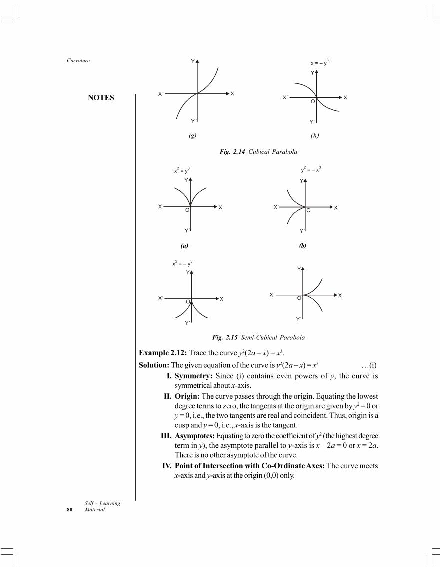
Curvature
NOTES
Self - Learning80 Material
Y
Y´
XX´X´
Y
x = – y3
O
Y´
X
(g) (h)
Fig. 2.14 Cubical Parabola
x = y32
Y
Y´
X´O X O XX´
Y
Y´
y = – x32
(a) (b)
Y
XO
x2 = – y
3
X´
Y´
Y
XOX´
Y´
Fig. 2.15 Semi-Cubical Parabola
Example 2.12: Trace the curve y2(2a – x) = x3.
Solution: The given equation of the curve is y2(2a – x) = x3 …(i)I. Symmetry: Since (i) contains even powers of y, the curve is
symmetrical about x-axis.II. Origin: The curve passes through the origin. Equating the lowest
degree terms to zero, the tangents at the origin are given by y2 = 0 ory = 0, i.e., the two tangents are real and coincident. Thus, origin is acusp and y = 0, i.e., x-axis is the tangent.
III. Asymptotes: Equating to zero the coefficient of y2 (the highest degreeterm in y), the asymptote parallel to y-axis is x – 2a = 0 or x = 2a.There is no other asymptote of the curve.
IV. Point of Intersection with Co-Ordinate Axes: The curve meetsx-axis and y-axis at the origin (0,0) only.
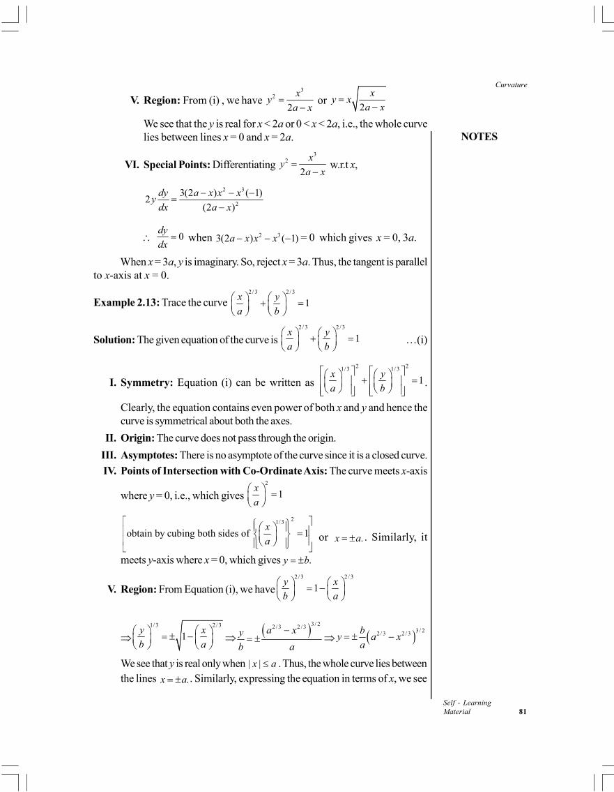
NOTES
Curvature
Self - LearningMaterial 81
V. Region: From (i) , we have 3
2
2
xy
a x
or
2
xy x
a x
We see that the y is real for x < 2a or 0 < x < 2a, i.e., the whole curvelies between lines x = 0 and x = 2a.
VI. Special Points: Differentiating 3
2
2
xy
a x
w.r.t x,
2 3
2
3(2 ) ( 1)2
(2 )
dy a x x xy
dx a x
0dy
dx when 2 33(2 ) ( 1)a x x x = 0 which gives x = 0, 3a.
When x = 3a, y is imaginary. So, reject x = 3a. Thus, the tangent is parallelto x-axis at x = 0.
Example 2.13: Trace the curve 2 / 3 2 / 3
1x y
a b
Solution: The given equation of the curve is 2 / 3 2 / 3
1x y
a b
…(i)
I. Symmetry: Equation (i) can be written as
2 21/3 1/ 3
1x y
a b
.
Clearly, the equation contains even power of both x and y and hence thecurve is symmetrical about both the axes.
II. Origin: The curve does not pass through the origin.
III. Asymptotes: There is no asymptote of the curve since it is a closed curve.
IV. Points of Intersection with Co-Ordinate Axis: The curve meets x-axis
where y = 0, i.e., which gives 2
1x
a
21/ 3
obtain by cubing both sides of 1x
a
or .x a . Similarly, it
meets y-axis where x = 0, which gives .y b
V. Region: From Equation (i), we have2 / 3 2 / 3
1y x
b a
1/ 3 2 / 3
1y x
b a
3/ 22 / 3 2 / 3a xy
b a
3/ 22 / 3 2 / 3b
y a xa
We see that y is real only when | |x a . Thus, the whole curve lies betweenthe lines .x a . Similarly, expressing the equation in terms of x, we see
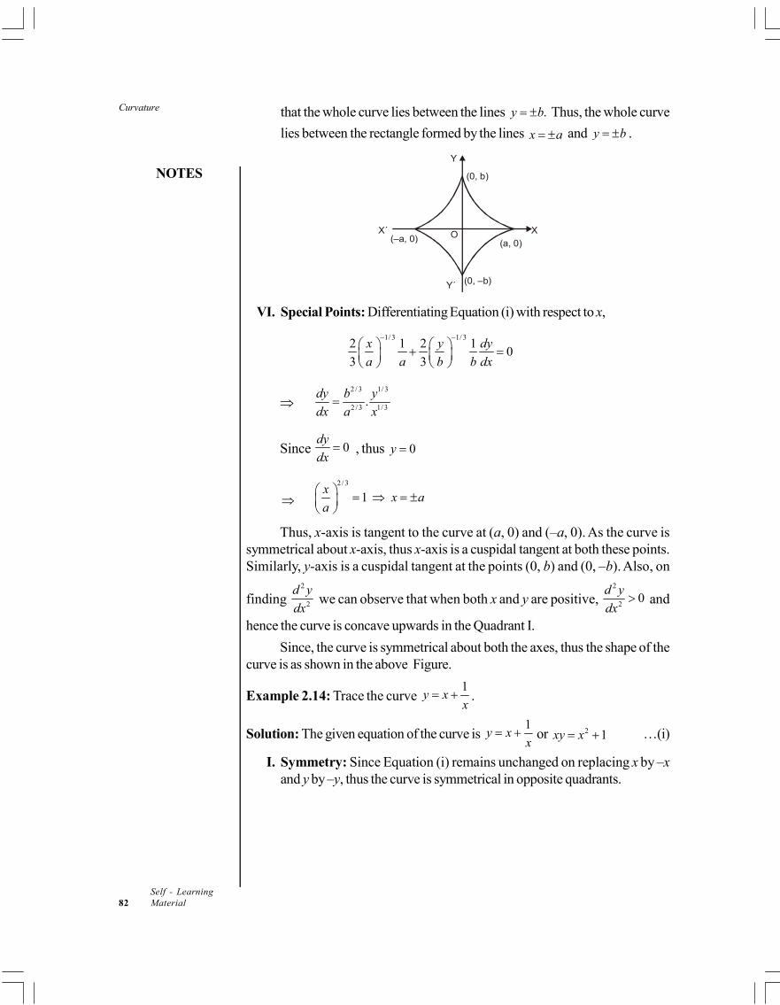
Curvature
NOTES
Self - Learning82 Material
that the whole curve lies between the lines .y b Thus, the whole curve
lies between the rectangle formed by the lines x a and y b .
Y
X´
Y´
XO
(0, b)
(–a, 0) (a, 0)
(0, –b)
VI. Special Points: Differentiating Equation (i) with respect to x,
1/ 3 1/ 32 1 2 1
03 3
x y dy
a a b b dx
2 / 3 1/ 3
2 /3 1/ 3.
dy b y
dx a x
Since 0dy
dx , thus 0y
2 / 3
1x
x aa
Thus, x-axis is tangent to the curve at (a, 0) and (–a, 0). As the curve issymmetrical about x-axis, thus x-axis is a cuspidal tangent at both these points.Similarly, y-axis is a cuspidal tangent at the points (0, b) and (0, –b). Also, on
finding 2
2
d y
dx we can observe that when both x and y are positive,
2
20
d y
dx and
hence the curve is concave upwards in the Quadrant I.
Since, the curve is symmetrical about both the axes, thus the shape of thecurve is as shown in the above Figure.
Example 2.14: Trace the curve 1
y xx
.
Solution: The given equation of the curve is 1
y xx
or 2 1xy x …(i)
I. Symmetry: Since Equation (i) remains unchanged on replacing x by –xand y by –y, thus the curve is symmetrical in opposite quadrants.
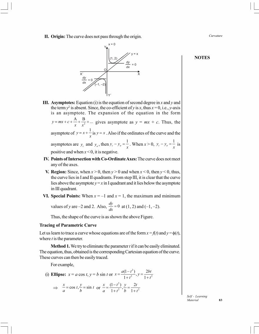
NOTES
Curvature
Self - LearningMaterial 83
II. Origin: The curve does not pass through the origin.
OXX´
Y´
(–1, –2)
dy
dx
dy
dx
= 0
= 0
(1, 2)
Yx = 0
y = x
III. Asymptotes: Equation (i) is the equation of second degree in x and y andthe term y2 is absent. Since, the co-efficient of y is x, thus x = 0, i.e., y-axisis an asymptote. The expansion of the equation in the form
2
A B...y mx c
x x gives asymptote as y = mx + c. Thus, the
asymptote of 1
y xx
is y x . Also if the ordinates of the curve and the
asymptotes are cy and ay , then1
c ay yx
. When x > 0, 1
c ay yx
is
positive and when x < 0, it is negative.
IV. Points of Intersection with Co-Ordinate Axes: The curve does not meetany of the axes.
V. Region: Since, when x > 0, then y > 0 and when x < 0, then y < 0, thus,the curve lies in I and II quadrants. From step III, it is clear that the curvelies above the asymptote y = x in I quadrant and it lies below the asymptotein III quadrant.
VI. Special Points: When x = –1 and x = 1, the maximum and minimum
values of y are –2 and 2. Also, 0dy
dx at (1, 2) and (–1, –2).
Thus, the shape of the curve is as shown the above Figure.
Tracing of Parametric Curve
Let us learn to trace a curve whose equations are of the form x = f(t) and y = (t),where t is the parameter.
Method 1. We try to eliminate the parameter t if it can be easily eliminated.The equation, thus, obtained is the corresponding Cartesian equation of the curve.These curves can then be easily traced.
For example,
(i) Ellipse: x = a cos t, y = b sin t or 2
2 2
(1 ) 2,
1 1
a t btx y
t t
cos , sinx y
t ta b or
2
2 2
(1 ) 2,
1 1
x t y t
a t b t
Curvature
NOTES
Self - Learning84 Material
Eliminating t by squaring and adding, we get2 2
2 21
x y
a b , which is an ellipse.
(ii) Circle: x = a cos t, y = a sin t or 2
2 2
(1 ) 2,
1 1
a t atx y
t t
Eliminating t by squaring and adding, we get
x2 + y2 = a2, which is a circle.
(iii) Cissoid: 3
2 sinsin ,
cos
tx a t y a
t
2sinx a t 3 3 6sinx a t
Or 2sinx a t 21 cosx a t 2cos 1x
ta
3sin
cos
ty a
t
62 2
2
sin
cos
ty a
t
3
2
1
x
ayx
a
3
2 xy
a x
,
which is called Cissoid.
(iv) Astroid: 3 3cos , sinx a t y a t
2 2 2 2
2 23 3 3 3cos , sinx a t y a t
Eliminating t by adding, we get2 2 2
3 3 3x y a , which is called Astroid.
(v) Hypocycloid: 3 3cos , sinx a t y b t
3 3cos , sinx y
t ta b
2 2
3 32 2cos , sin
x yt t
a b
Eliminating t by squaring and adding, we get2 2
3 31
x y
a b
, which is called Hypocycloid.
(vi) Simple Curve: 2 31,
3x t y t t
2
3 2 2 21 11
3 3y t t y t t
Eliminating t by putting t2 = x, we get2
2 13
xy x
9y2 = x(x – 3)2, which is a form of a simple curve.
NOTES
Curvature
Self - LearningMaterial 85
(vii) Folium of Descartes’: 2
3 3
3 3,
1 1
at atx y
t t
Dividing, we get y
tx
Putting this value of t in 3
3
1
atx
t
, we get
x3 + y3 = 3axy, which is called Folium of Descartes’.
(viii) Lemniscate of Bernoulli: 3 3
4 4
( ) ( ),
1 1
a t t a t tx y
t t
Eliminating t, we get (x2 + y2)2 = a2(x2 – y2), which is called Lemniscate ofBernoulli.
Method 2. When the parameter t cannot be easily eliminated, then we adopt thefollowing steps to trace the curve:
I. Symmetry:
(i) Symmetry about x-Axis: The curve is symmetrical about x-axis if byreplacing t by –t or t by – t, y changes to –y and x remains unchanged.For example, the parabola x = at2, y = 2at is symmetrical about x-axis.
(ii) Symmetry about y-Axis: The curve is symmetrical about y-axis if byreplacing t by –t or t by – t, x changes to –x and y remains unchanged.For example, the ellipse x = a cos t, y = b sin t is symmetrical abouty-axis.
(iii) Symmetry in Opposite Quadrants: The curve is symmetrical in oppositequadrants if by replacing t by –t, x changes to –x and y changes to –y.
For example, the rectangular hyperbola x = ct, y = c
t is symmetrical in
opposite quadrants.
II. Origin: Find whether the curve passes through the origin. The curve passesthrough the origin if the same real value of t satisfies both f(t) = 0 and (t) = 0.
III. Asymptotes:
(i) Asymptotes Parallel to Co-Ordinate Axes: Obtain the asymptotesparallel to x-axis by finding the values b
1, b
2, … to which y tends as x
or x – . We get y = b1, y = b
2 as asymptotes. Similarly, obtain the
asymptotes parallel to y-axis by finding the values a1, a
2, … to which x
tends as y or y – . We get x = a1, x = a
2 as asymptotes.
(ii) Oblique Asymptotes: y = mx + c is an oblique asymptote if for somevalue of t (say t t
0), both x and y tends to and
0 0
lim and lim( )t t t t
ym y mx c
x .
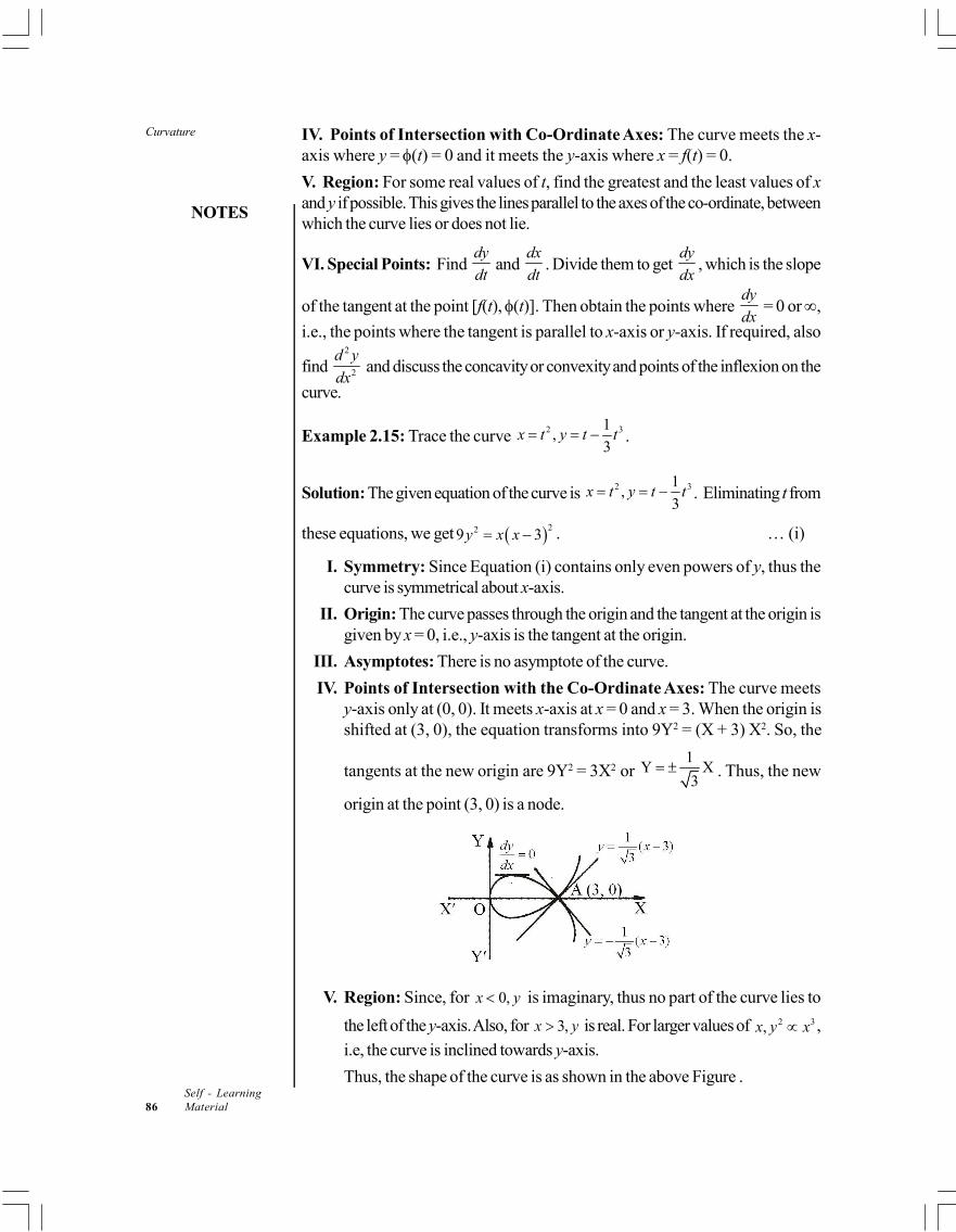
Curvature
NOTES
Self - Learning86 Material
IV. Points of Intersection with Co-Ordinate Axes: The curve meets the x-axis where y = (t) = 0 and it meets the y-axis where x = f(t) = 0.
V. Region: For some real values of t, find the greatest and the least values of xand y if possible. This gives the lines parallel to the axes of the co-ordinate, betweenwhich the curve lies or does not lie.
VI. Special Points: Find dy
dt and
dx
dt. Divide them to get
dy
dx, which is the slope
of the tangent at the point [f(t), (t)]. Then obtain the points where dy
dx = 0 or ,
i.e., the points where the tangent is parallel to x-axis or y-axis. If required, also
find 2
2
d y
dx and discuss the concavity or convexity and points of the inflexion on the
curve.
Example 2.15: Trace the curve 2 31,
3x t y t t .
Solution: The given equation of the curve is 2 31,
3x t y t t . Eliminating t from
these equations, we get 229 3y x x . … (i)
I. Symmetry: Since Equation (i) contains only even powers of y, thus thecurve is symmetrical about x-axis.
II. Origin: The curve passes through the origin and the tangent at the origin isgiven by x = 0, i.e., y-axis is the tangent at the origin.
III. Asymptotes: There is no asymptote of the curve.
IV. Points of Intersection with the Co-Ordinate Axes: The curve meetsy-axis only at (0, 0). It meets x-axis at x = 0 and x = 3. When the origin isshifted at (3, 0), the equation transforms into 9Y2 = (X + 3) X2. So, the
tangents at the new origin are 9Y2 = 3X2 or 1
Y X3
. Thus, the new
origin at the point (3, 0) is a node.
V. Region: Since, for 0,x y is imaginary, thus no part of the curve lies to
the left of the y-axis. Also, for 3,x y is real. For larger values of 2 3,x y x ,
i.e, the curve is inclined towards y-axis.
Thus, the shape of the curve is as shown in the above Figure .
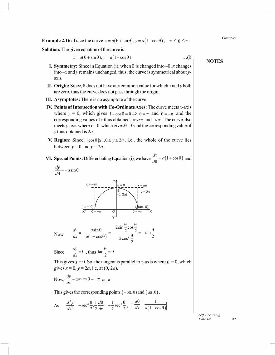
NOTES
Curvature
Self - LearningMaterial 87
Example 2.16: Trace the curve sin , 1 cosx a y a , – .
Solution: The given equation of the curve is
sin , 1 cosx a y a …(i)
I. Symmetry: Since in Equation (i), when is changed into –, x changesinto –x and y remains unchanged, thus, the curve is symmetrical about y-axis.
II. Origin: Since, does not have any common value for which x and y bothare zero, thus the curve does not pass through the origin.
III. Asymptotes: There is no asymptote of the curve.
IV. Points of Intersection with Co-Ordinate Axes: The curve meets x-axiswhere y = 0, which gives 1 cos 0 and – and thecorresponding values of x thus obtained are a and –a . The curve alsomeets y-axis where x = 0, which gives = 0 and the corresponding value ofy thus obtained is 2a.
V. Region: Since, | cos | 1,0 2y a , i.e., the whole of the curve liesbetween y = 0 and y = 2a.
VI. Special Points: Differentiating Equation (i), we have 1 cosdx
ad
and
sindy
ad
x = –aπ
(–a , 0)π
0 = –π OX´
Y´
X
Yθ = 0 x = aπ
y = 2aB(0, 2a)
A0 = –π
(a , 0)π
Now, sin
1 cos
dy a
dx a
2
2sin cos2 2 tan
22cos2
Since 0dy
dx , thus tan 0
2
This gives = 0. So, the tangent is parallel to x-axis where = 0, whichgives x = 0, y = 2a, i.e, at (0, 2a).
Now,dy
dx or
This gives the corresponding points ,0a and ,0a .
As2
2 42
1 1sec . sec
2 2 2 2
d y d
dx dx
,
1
1 cos
d
dx a
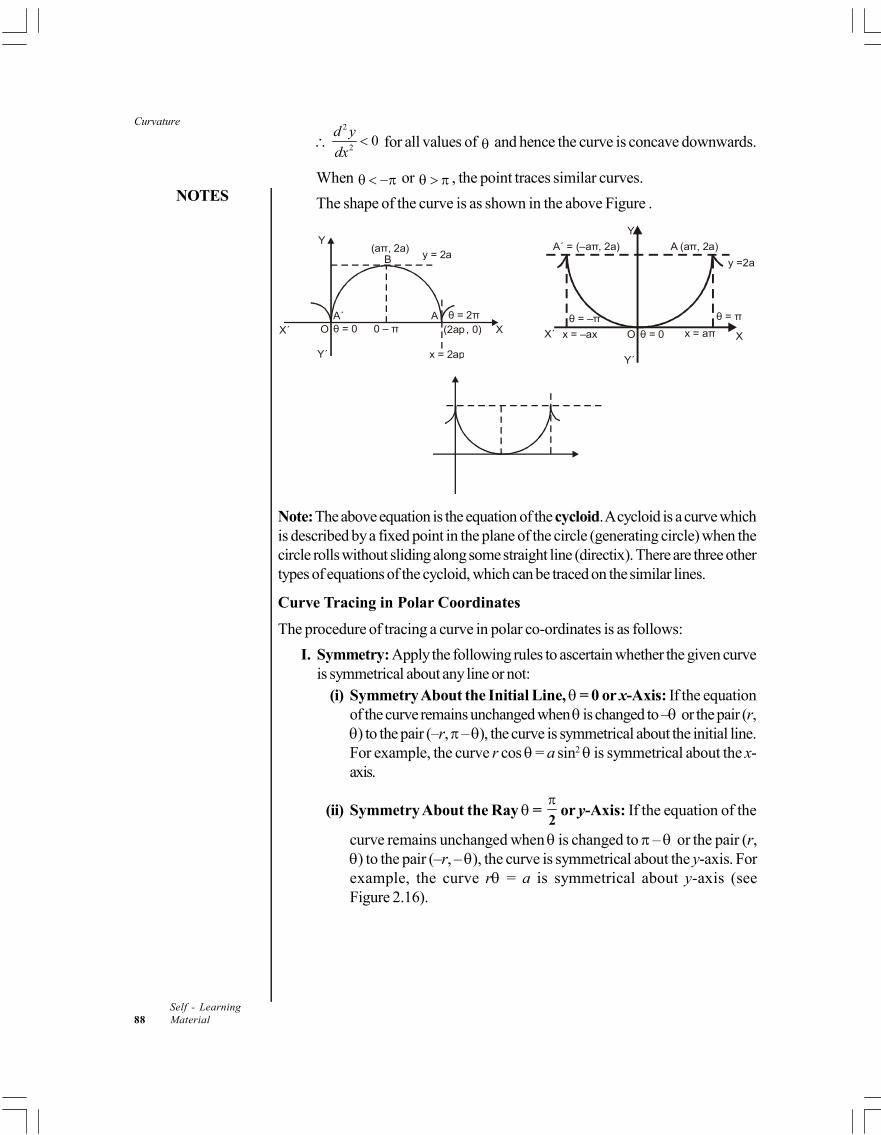
Curvature
NOTES
Self - Learning88 Material
2
20
d y
dx for all values of and hence the curve is concave downwards.
When or , the point traces similar curves.
The shape of the curve is as shown in the above Figure .
θ = 0
Y
B y = 2a
X´
Y´
O 0 – πA´ A
(a , 2a)π
θ = 2π(2ap , 0)
x = 2ap
X X´ X
A (aπ, 2a)
y =2a
θ = –π
A´ , 2a) = (–aπ
x = –ax θ = 0O x = aπ
θ = π
Y´
Y
Note: The above equation is the equation of the cycloid. A cycloid is a curve whichis described by a fixed point in the plane of the circle (generating circle) when thecircle rolls without sliding along some straight line (directix). There are three othertypes of equations of the cycloid, which can be traced on the similar lines.
Curve Tracing in Polar Coordinates
The procedure of tracing a curve in polar co-ordinates is as follows:
I. Symmetry: Apply the following rules to ascertain whether the given curveis symmetrical about any line or not:
(i) Symmetry About the Initial Line, = 0 or x-Axis: If the equationof the curve remains unchanged when is changed to – or the pair (r,) to the pair (–r, – ), the curve is symmetrical about the initial line.For example, the curve r cos = a sin2 is symmetrical about the x-axis.
(ii) Symmetry About the Ray = 2
or y-Axis: If the equation of the
curve remains unchanged when is changed to – or the pair (r,) to the pair (–r, – ), the curve is symmetrical about the y-axis. Forexample, the curve r = a is symmetrical about y-axis (seeFigure 2.16).
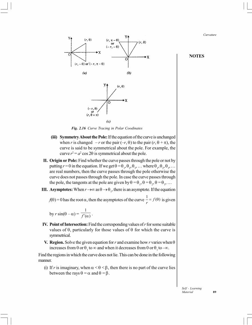
NOTES
Curvature
Self - LearningMaterial 89
(a) (b)
(c)
Fig. 2.16 Curve Tracing in Polar Coodinates
(iii) Symmetry About the Pole: If the equation of the curve is unchangedwhen r is changed – r or the pair (–r, ) to the pair (r, + ), thecurve is said to be symmetrical about the pole. For example, thecurve r2 = a2 cos 2 is symmetrical about the pole.
II. Origin or Pole: Find whether the curve passes through the pole or not byputting r = 0 in the equation. If we get =
1,
2,
3, … where
1,
2,
3, …
are real numbers, then the curve passes through the pole otherwise thecurve does not passes through the pole. In case the curve passes throughthe pole, the tangents at the pole are given by =
1, =
2, =
3, …
III. Asymptotes: When r as 1, there is an asymptote. If the equation
f() = 0 has the root , then the asymptotes of the curve 1
( )fr is given
by r sin( – ) = 1
( )f .
IV. Point of Intersection: Find the corresponding values of r for some suitablevalues of , particularly for those values of for which the curve issymmetrical.
V. Region. Solve the given equation for r and examine how r varies when increases from 0 or
1 to and when it decreases from 0 or
1 to –.
Find the regions in which the curve does not lie. This can be done in the followingmanner.
(i) If r is imaginary, when < < , then there is no part of the curve liesbetween the rays = and = .
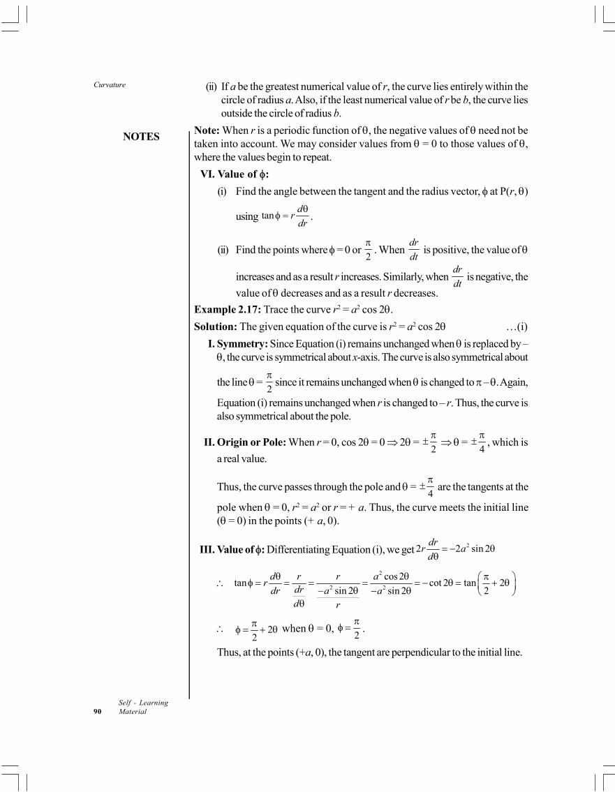
Curvature
NOTES
Self - Learning90 Material
(ii) If a be the greatest numerical value of r, the curve lies entirely within thecircle of radius a. Also, if the least numerical value of r be b, the curve liesoutside the circle of radius b.
Note: When r is a periodic function of , the negative values of need not betaken into account. We may consider values from = 0 to those values of ,where the values begin to repeat.
VI. Value of :
(i) Find the angle between the tangent and the radius vector, at P(r, )
using tand
rdr
.
(ii) Find the points where = 0 or 2
. When
dr
dt is positive, the value of
increases and as a result r increases. Similarly, when dr
dt is negative, the
value of decreases and as a result r decreases.
Example 2.17: Trace the curve r2 = a2 cos 2.
Solution: The given equation of the curve is r2 = a2 cos 2 …(i)
I. Symmetry: Since Equation (i) remains unchanged when is replaced by –, the curve is symmetrical about x-axis. The curve is also symmetrical about
the line = 2
since it remains unchanged when is changed to – . Again,
Equation (i) remains unchanged when r is changed to – r. Thus, the curve isalso symmetrical about the pole.
II. Origin or Pole: When r = 0, cos 2 = 0 2 = 2
=
4
, which is
a real value.
Thus, the curve passes through the pole and = 4
are the tangents at the
pole when = 0, r2 = a2 or r = + a. Thus, the curve meets the initial line( = 0) in the points (+ a, 0).
III. Value of : Differentiating Equation (i), we get 22 2 sin 2dr
r ad
2
2 2
cos 2tan cot 2 tan 2
sin 2 sin 2 2
d r r ar
dr adr ad r
22
when = 0,
2
.
Thus, at the points (+a, 0), the tangent are perpendicular to the initial line.
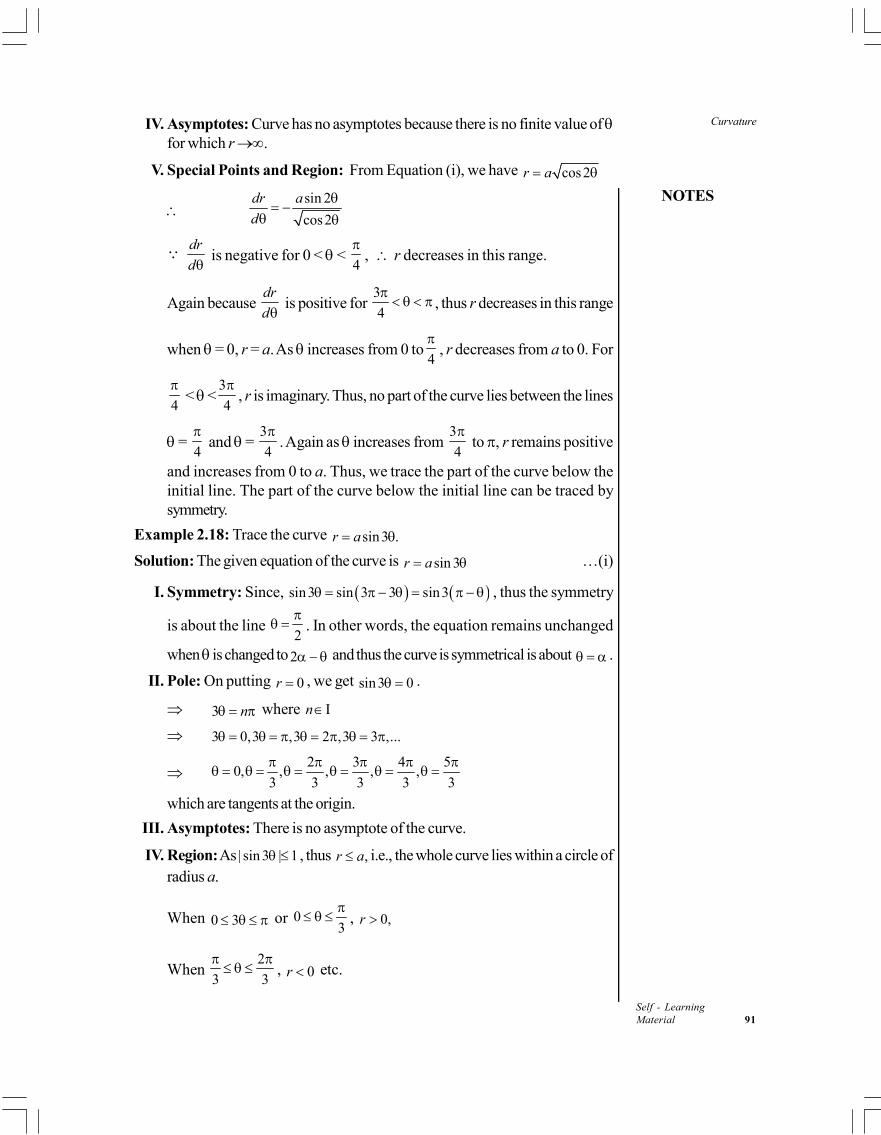
NOTES
Curvature
Self - LearningMaterial 91
IV. Asymptotes: Curve has no asymptotes because there is no finite value of for which r .
V. Special Points and Region: From Equation (i), we have cos2r a
sin 2
cos2
dr a
d
dr
d is negative for 0 < <
4
, r decreases in this range.
Again becausedr
d is positive for
3
4
, thus r decreases in this range
when = 0, r = a. As increases from 0 to4
, r decreases from a to 0. For
4
< <
4
, r is imaginary. Thus, no part of the curve lies between the lines
= 4
and =
4
. Again as increases from
4
to , r remains positive
and increases from 0 to a. Thus, we trace the part of the curve below theinitial line. The part of the curve below the initial line can be traced bysymmetry.
Example 2.18: Trace the curve sin3 .r a
Solution: The given equation of the curve is sin 3r a …(i)
I. Symmetry: Since, sin3 sin 3 3 sin3 , thus the symmetry
is about the line 2
. In other words, the equation remains unchanged
when is changed to 2 and thus the curve is symmetrical is about .
II. Pole: On putting 0r , we get sin3 0 .
3 n where In
3 0,3 ,3 2 ,3 3 ,...
2 3 4 5
0, , , , ,3 3 3 3 3
which are tangents at the origin.
III. Asymptotes: There is no asymptote of the curve.
IV. Region: As | sin 3 | 1 , thus ,r a i.e., the whole curve lies within a circle ofradius a.
When 0 3 or 03
, 0,r
When 2
3 3
, 0r etc.
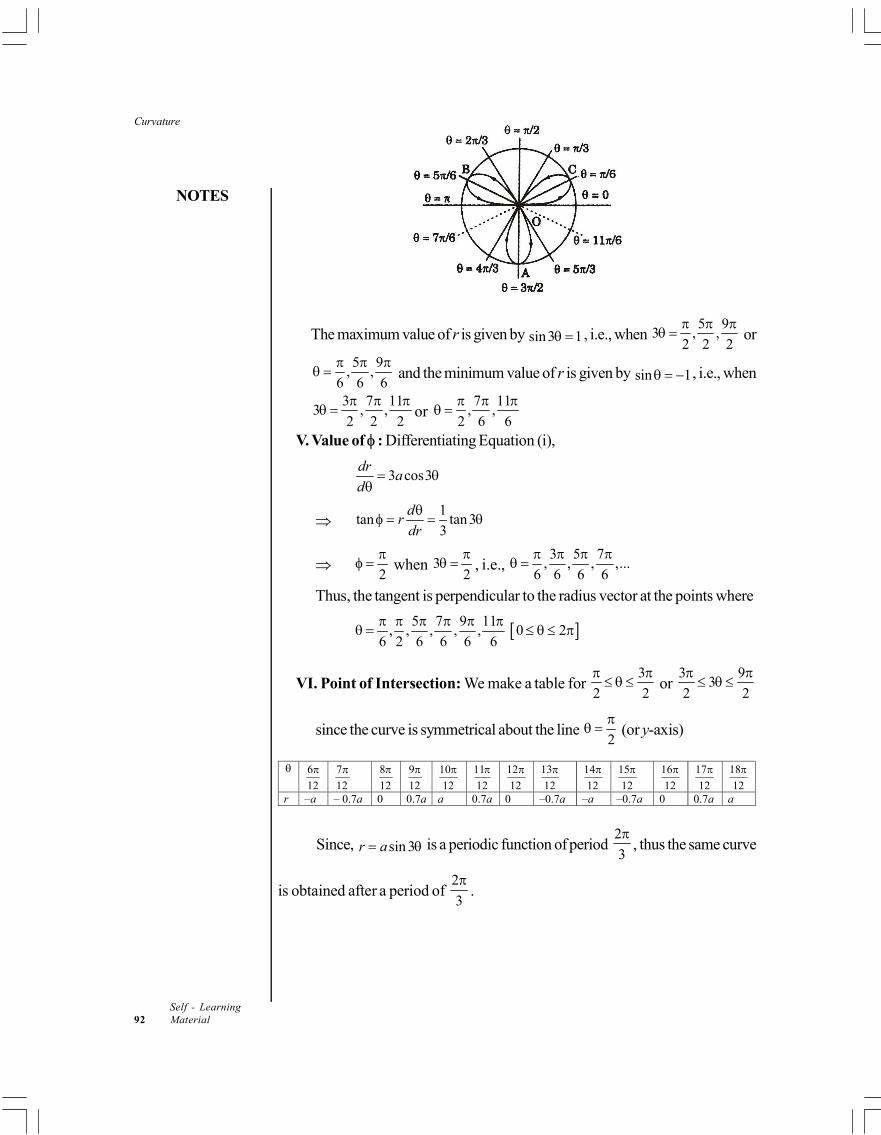
Curvature
NOTES
Self - Learning92 Material
The maximum value of r is given by sin3 1 , i.e., when 5 9
3 , ,2 2 2
or
5 9, ,
6 6 6
and the minimum value of r is given by sin 1 , i.e., when
3 7 113 , ,
2 2 2
or
7 11, ,
2 6 6
V. Value of : Differentiating Equation (i),
3 cos3dr
ad
1
tan tan 33
dr
dr
2
when 3
2
, i.e.,
3 5 7, , , ,...
6 6 6 6
Thus, the tangent is perpendicular to the radius vector at the points where
5 7 9 11, , , , , 0 2
6 2 6 6 6 6
VI. Point of Intersection: We make a table for 3
2 2
or
3 93
2 2
since the curve is symmetrical about the line 2
(or y-axis)
6
12
7
12
8
12
9
12
10
12
11
12
12
12
13
12
14
12
15
12
16
12
17
12
18
12
r –a – 0.7a 0 0.7a a 0.7a 0 –0.7a –a –0.7a 0 0.7a a
Since, sin 3r a is a periodic function of period 2
3
, thus the same curve
is obtained after a period of 2
3
.
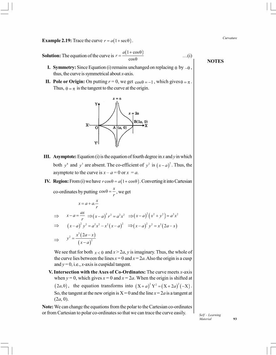
NOTES
Curvature
Self - LearningMaterial 93
Example 2.19: Trace the curve 1 secr a .
Solution: The equation of the curve is 1 cos
cos
ar
…(i)
I. Symmetry: Since Equation (i) remains unchanged on replacing by – ,thus, the curve is symmetrical about x-axis.
II. Pole or Origin: On putting r = 0, we get cos 1 , which gives .Thus, is the tangent to the curve at the origin.
III. Asymptote: Equation (i) is the equation of fourth degree in x and y in which
both 4y and 3y are absent. The co-efficient of 2y is 2x a . Thus, the
asymptote to the curve is x – a = 0 or x = a.
IV. Region: From (i) we have cos 1 cosr a . Converting it into Cartesian
co-ordinates by putting cosx
r , we get
.x
x a ar
ax
x ar
2 2 2 2x a r a x 2 2 2 2 2x a x y a x
2 22 2 2 2x a y a x x x a 2 2 3 2x a y x a x
32
2
2x a xy
x a
We see that for both 0x and x > 2a, y is imaginary. Thus, the whole ofthe curve lies between the lines x = 0 and x = 2a. Also the origin is a cuspand y = 0, i.e., x-axis is cuspidal tangent.
V. Intersection with the Axes of Co-Ordinates: The curve meets x-axiswhen y = 0, which gives x = 0 and x = 2a. When the origin is shifted at
2 ,0a , the equation transforms into 2 22X Y X 2 Xa a .
So, the tangent at the new origin is X = 0 and the line x = 2a is a tangent at(2a, 0).
Note: We can change the equations from the polar to the Cartesian co-ordinatesor from Cartesian to polar co-ordinates so that we can trace the curve easily.
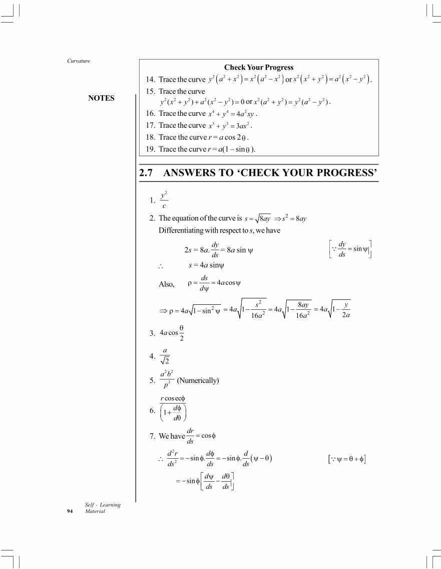
Curvature
NOTES
Self - Learning94 Material
Check Your Progress
14. Trace the curve 2 2 2 2 2 2y a x x a x or 2 2 2 2 2 2x x y a x y .
15. Trace the curve2 2 2 2 2 2( ) ( ) 0y x y a x y or 2 2 2 2 2 2( ) ( )x a y y a y .
16. Trace the curve 4 4 24x y a xy .
17. Trace the curve 3 3 23x y ax .
18. Trace the curve r = a cos 2 .
19. Trace the curve r = a(1 – sin ).
2.7 ANSWERS TO ‘CHECK YOUR PROGRESS’
1.2y
c
2. The equation of the curve is 28 8s ay s ay
Differentiating with respect to s, we have
2s = 8a.dy
ds= 8a sin sin
dy
ds
s = 4a sin
Also, 4 cosds
ad
24 1 sina 2
2 2
84 1 4 1
16 16
s aya a
a a 4 1
2
ya
a
3. 4 cos2
a
4.2
a
5.2 2
3
a b
p (Numerically)
6.
cosec
1θ
rdd
7. We have cosdr
ds
2
2sin . sin .
d r d d
ds ds ds
sind d
ds ds
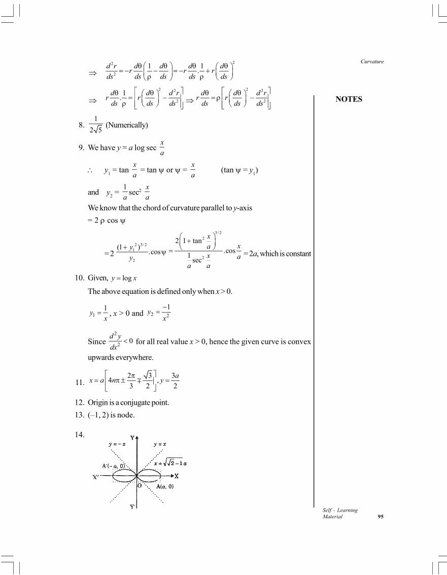
NOTES
Curvature
Self - LearningMaterial 95
22
2
1 1.
d r d d d dr r r
ds ds ds ds ds
2 2
2
1.
d d d rr r
ds ds ds
2 2
2
d d d rr r
ds ds ds
8.1
2 5 (Numerically)
9. We have y = a log sec x
a
y1 = tan
x
a = tan or =
x
a(tan = y
1)
and y2 =
1
asec2
x
a
We know that the chord of curvature parallel to y-axis
= 2 cos
= 2 2 3/ 2
1
2
(1 ).cos
y
y
3/ 22
2
2 1 tan.cos
1sec
xxa
x aa a
= 2a, which is constant
10. Given, logy x
The above equation is defined only when x > 0.
11
yx
, x > 0 and 2 2
1y
x
Since 2
20
d y
dx for all real value x > 0, hence the given curve is convex
upwards everywhere.
11.2 3 3
4 ,3 2 2
ax a n y
12. Origin is a conjugate point.
13. (–1, 2) is node.
14.
X
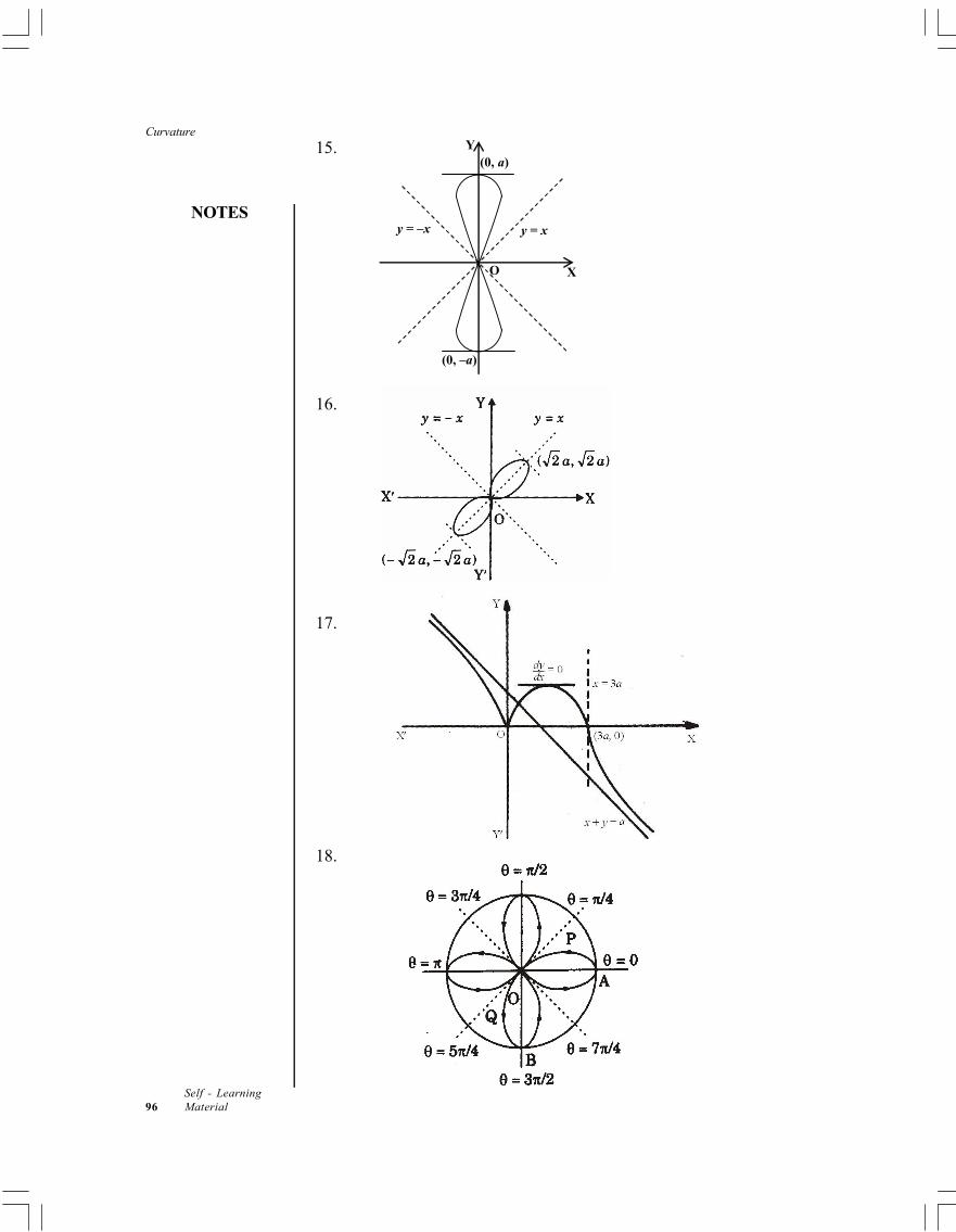
Curvature
NOTES
Self - Learning96 Material
15.
X
Y
O
(0, a)
y = x y = –x
(0, –a)
16.
17.
18.
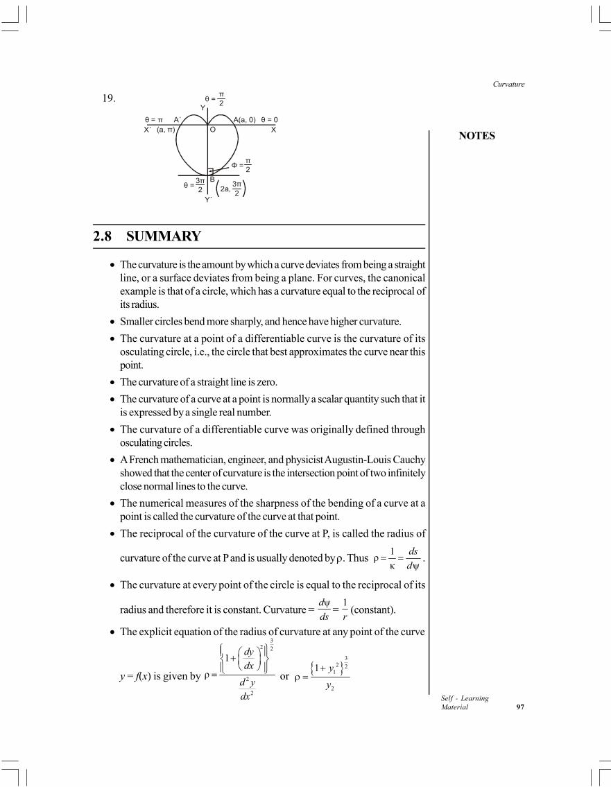
NOTES
Curvature
Self - LearningMaterial 97
19. π2
π2
32π
θ = 32π
2a,
θ =
Ф =
Y
θ = 0θ π = (a, )π O
B
XX´A´ A(a, 0)
Y´
2.8 SUMMARY
The curvature is the amount by which a curve deviates from being a straightline, or a surface deviates from being a plane. For curves, the canonicalexample is that of a circle, which has a curvature equal to the reciprocal ofits radius.
Smaller circles bend more sharply, and hence have higher curvature.
The curvature at a point of a differentiable curve is the curvature of itsosculating circle, i.e., the circle that best approximates the curve near thispoint.
The curvature of a straight line is zero.
The curvature of a curve at a point is normally a scalar quantity such that itis expressed by a single real number.
The curvature of a differentiable curve was originally defined throughosculating circles.
A French mathematician, engineer, and physicist Augustin-Louis Cauchyshowed that the center of curvature is the intersection point of two infinitelyclose normal lines to the curve.
The numerical measures of the sharpness of the bending of a curve at apoint is called the curvature of the curve at that point.
The reciprocal of the curvature of the curve at P, is called the radius of
curvature of the curve at P and is usually denoted by . Thus 1
ρκ
ds
d
.
The curvature at every point of the circle is equal to the reciprocal of its
radius and therefore it is constant. Curvature = ψd
ds=
1
r(constant).
The explicit equation of the radius of curvature at any point of the curve
y = f(x) is given by
32 2
2
2
1
ρ
dy
dx
d y
dx
or
3
2 21
2
1 y
y
Curvature
NOTES
Self - Learning98 Material
The radius of curvature defined by parametric equations x = f(t), y = (t) is
given by 2 2 3/ 2( ' ' )
ρ' '' ' ''
x y
x y y x
.
The implicit equation of the radius of curvature at any point of the curve
f(x,y) = 0 is given by
32 2 2
2 2ρ
2
x y
xx y x y xy yy x
f f
f f f f f f f
.
Radius of Curvature when x and y are function of s is given by the equation2 2
2ρdx dy
d d
.
The graph of f is concave downwards or convex upwards on [a, b] if,
throughout (a, b), it lies below the tangent lines of f, i.e., if f is decreasingin the interval.
The curve is concave or convex in upwards direction depends upon
whether c ty y > 0 or c ty y < 0, i.e., 2
20
d y
dx or
2
20
d y
dx
A point of inflexion is a point on a curve at which the curve changes frombeing concave upwards to concave downwards or vice-versa.
Singular point is a point on a curve at which the curve shows an extraordinaryor unusual behaviour.
If more than one branch of a curve passes through a point on the curve,then this point is said to be multiple point of the curve.
If two branches of the curve pass through a point on the curve, then thispoint is called a double point.
If the two tangents at the double point are real and distinct, then the doublepoint is known as a node.
If there are no real points of the curve in the neighbourhood of the point,then this point P is called a conjugate or an isolated point of the curve.
The graph of f is concave upwards or convex downwards on [a, b] if,
throughout (a, b), it lies above the tangent lines of f, i.e., if f is increasingin the interval.
If the equation of a curve remains unaltered when y is changed to – y, i.e.,if all the powers of y in the given equation are even, the curve is symmetricalabout the x-axis.
If the equation of a curve remains unaltered when x is changed to – x, i.e.,if all the powers of x are even in the given equation, the curve is symmetricalabout the y-axis.
NOTES
Curvature
Self - LearningMaterial 99
If all the powers of both x and y are even in the given equation, the curve issymmetrical about both the axes.
If the equation of the curve remains unchanged when x and y are changedto –x and –y, respectively, the curve is symmetrical in opposite quadrants.
If the equation of the curve is unchanged when x and y are interchanged(i.e., x is changed to y and y to x), the curve is symmetrical about the liney = x.
If the equation of the curve is unchanged when x is changed to –y and y ischanged to –x, the curve is symmetrical about the line y = –x.
A cycloid is a curve which is described by a fixed point in the plane of thecircle (generating circle) when the circle rolls without sliding along some straightline. There are three other types of equations of the cycloid, which can betraced on the similar lines.
2.9 KEY TERMS
Curvature: It is the numerical measure of the sharpness of the bending of acurve at a point.
Radius of curvature: It is the reciprocal of the curvature of the curve at P,and is usually denoted by .
Double point: If two branches of the curve pass through a point on thecurve, then this point is called a double point.
Inflexion point: It is a point on a curve at which the curve changes frombeing concave upwards to concave downwards or vice-versa.
Curve tracing: It means to find the approximate shape of a curve withoutplotting a large number of points.
Cycloid: It is a curve which is described by a fixed point in the plane of thecircle (generating circle) when the circle rolls without sliding along somestraight line.
2.10 SELF-ASSESSMENT QUESTIONS ANDEXERCISES
Short-Answer Questions
1. Find the radius of curvature at ,s for each of the following curves:
(i) log tan sec tan secs a a (ii) 28 sin6
s a
2. Find the radius of curvature at the given point for the following curves:
(i) 2xy c at the point (x, y) (ii) 4sin sin 2y x x at 2
x
Curvature
NOTES
Self - Learning100 Material
3. Show that the radius of curvature at any point of the astroide3 3cos , sinx a y a is equal to three times the length of the perpendicular
from the origin to the tangent.
4. The tangents at two points P, Q on the cycloid
sin ; 1 cosx a y a are at right angles. Show that if 1 2, are
the radii of curvature at these points then 2 2 21 2 16 .a
5. Prove that for an ellipse 2 2
2 21
x y
a b
2 2
3
a b
p , where p is the length of the
perpendicular from the centre upon the tangent at the point P(x, y).
6. Show that the radius of curvature at any point P(x,y) of the curve2 / 3 2 / 3 2 / 3x y a is given by 3 27 .axy
7. Show that for the cardioid 1 cosr a , the radius of curvature
4
cos3 2
a and
2 8
9
a
r
8. Find the radius of curvature for the following curves at (r, ):
(i) cosr a n (ii) 2 2cos2r a (iii) sinm mr a m
9. Find the radius of curvature for the following curves at (p, r):
(i) the cardioid 2 32ap r (ii)4
22 2
rp
r a
10. Find the radius of curvature for the following curves at ,p :
(i) the circle 1 sinp a (ii) 1 1 sin1
m m
m m mp a
m
11. Show that the radius of curvature for the curve 2 2
1cosr a a
a r
is
2 2r a .
12. Show that the radius of curvature of the curve r2 = a2 cos 2 at the point
where the tangent is parallel to x-axis is 2
3
a.
13. Find the radius of curvature at the origin for the following curves:
(i) 3 2 22 6 0x y x y
(ii) 2 22y x x xy y
NOTES
Curvature
Self - LearningMaterial 101
(iii) 2 2 31 2 1 2 3 1 .... 0a x a y b x b xy b y c x
(iv) 2 2 3 4 53 4 5 0y xy x x x y y
(v) 2 2 3a y x x
14. Show that for the hyperbola 2 2
2 21,
x y
a b whose parametric equations are
sec , tanx a y b , the centre of curvature at any point ‘ ’ is
2 2 2 23 3sec , tan
a b a b
a b
and the equation of its evolute is
2 / 32 / 3 2 /3 2 2ax by a b .
15. Show that the chord of curvature parallel to y-axis for the catenary
coshx
y cc
is double the ordinate of the point and the chord of curvature
parallel to x-axis is 2
sinhx
cc
.
Long-Answer Questions
1. Find the nature of the origin on the curves given below:
(i) 3 3 2y x ax
(ii) 4 4 4 0x y xy
(iii) 4 2 2 2 2 0x ax y axy a y
(iv) 2 2 2 2 34a y a x x
2. Determine the position and nature of double points on the curves givenbelow:
(i) 2 2( 2) ( 1)x y y
(ii) 2 6( ) 0y x x
(iii) 4 3 3 2 2 2 2 44 2 4 3 0x ax ay a x a y a
(iv) 2 3( 6) ( 2) 9y y x x
(v) 3 2 3 2 24 4 1 0x xy y x y x y
(vi) 2 2 siny x x
3. Find the equations of the tangents at the multiple point of the
curve 2 2( 2) ( 1)x y y .
Curvature
NOTES
Self - Learning102 Material
4. Prove that the curve 2 tanx
y bxa
has a conjugate point or a node at the
origin according as a and b have unlike or like signs.
5. Discuss the convexity or concavity in the upward direction of the curve
(sin cos )xy e x x for0 2x .
6. Determine the intervals of x for which the curve 2 4 5 xy x x e is
(i) Concave Upwards(ii) Concave Downwards
7. Find the points of inflexion for the following curve:
(i) 3(log )x y
(ii) sinx
y ca
(iii) 2 354 ( 5) ( 10)y x x
(iv) ( 1)( 2)( 3)x y y y
8. Show that the abscissa of the points of inflexion of the curve 2 ( )y f x ,
satisfy the equation
2( ) 2 ( ) ( )f x f x f x .
9. Show that the points of inflexion of the curve 2 2( ) ( )y x a x b lies on
the line 3x + a = 4b.
10. Show that the abscissa of the points of inflexion of the curve2 2
cos , sin is .a b
x a b y a ba
11. Trace the following curves in Cartesian co-ordinates:
(i) 9ay2 = x(x – 3a2)
(ii) a2y2 = x2(a2 – x2)
(iii) (a2 + x2)y = a2x
(iv) x2 = y2(x + a)3
(v) y2 = (x – 2)2(x – 5)
(vi) xy2 = 4a2 (2a – x)
(vii) x2 = (y – 1)(y – 2)(y – 3)
(viii)2
2
1
1
xy
x
NOTES
Curvature
Self - LearningMaterial 103
(ix) y(x2 + 4a)2 = 8a3
(x) (x2 – a2)(y2 – b2) = a2b2
(xi) y2(a + x) = x2(a – x) or x(x2 + y2) = a(x2 – y2)
(xii) x3 + y3 = 3axy
(xiii) x2y2 = a2 (y2 – x2)
(xiv) x2/3 + y2/3 = a2/3
(xv) y = x3 – x
(xvi) 3
1xy
x
12. Trace the following curves in parametric form:
(i) x = a( – sin ), y = a(1 – cos )
(ii)2
3 3
3 3,
1 1
at atx y
t t
(iii)3 3
4 4
( ) ( ),
1 1
a t t a t tx y
t t
(iv)2 2
2 2
(1 ) (1 ),
1 1
a t at tx y
t t
(v) 2cos log tan , sin2 2
a tx a t y a t
(vi) x = a[cos – log( 1+ cos )], y = a sin
13. Trace the following curves in polar co-ordinates.
(i) r = a(1 + sin )
(ii) r = a(1 – cos )
(iii) r = 3(1 + cos )
(iv) r = a
(v) r = a sin 2(vi) r = a cos 3
(vii)2
21
ar
(viii) r2 cos = a2 sin 3
(ix) r2 cos 2 = a2 or x2 – y2 = a2
(x) x5 + y5 = 5a2x2y [Hint: change equation into polar co-ordinates].
2.11 FURTHER READING
Prasad, Gorakh. 2016. Differential Calculus. Allahabad: Pothishala Private Ltd.
Prasad, Gorakh. 2015. Integral Calculus. Allahabad: Pothishala Private Ltd.
Curvature
NOTES
Self - Learning104 Material
Murray, Daniel A. 1967. Introductory Course in Differential Equations. India:Orient Longman.
Coddington, Earl A. 1987. An Introduction to Ordinary Differential Equations.New Delhi: Prentice Hall of India.
Coddington, Earl A. and N. Levinson. 1972. Theory of Ordinary DifferentialEquations. New Delhi: Tata Mc Graw-Hill.
Boyce, W.E. and Richard C. DiPrima. 1986. Elementary Differential Equationsand Boundary Value Problems. New York: John Wiley and Sons, Inc.
Gelfand, J.M. and S.V. Fomin. 1963. Calculus of Variations. New Jersey: PrenticeHall.
Ross, S. L. 1984. Differential Equations, 3rd Edition. New York: John Wileyand Sons.
Somasundaram, D. 2002. Ordinary Differential Equations. Chennai: NarosaPublishing House.
NOTES
Integration of TranscendentalFunctions, Reduction,
Quadrature and Rectification
Self - LearningMaterial 105
UNIT 3 INTEGRATION OFTRANSCENDENTALFUNCTIONS, REDUCTION,QUADRATURE ANDRECTIFICATION
Structure
3.0 Introduction3.1 Objectives3.2 Integration and Definite Integrals3.3 Reduction Formula
3.3.1 Walli’s Formula
3.3.2 Reduction Formulae for tann x dx and cotn x dx
3.3.3 Gamma Function3.4 Integration of Transcendental Functions3.5 Quadrature3.6 Rectification3.7 Answers to ‘Check Your Progress’3.8 Summary3.9 Key Terms
3.10 Self-Assessment Questions and Exercises3.11 Further Reading
3.0 INTRODUCTION
In mathematics, an integral assigns numbers to functions in a way that can describedisplacement, area, volume, and other concepts that arise by combining infinitesimaldata. Integration is one of the two main operations of calculus, with its inverseoperation, differentiation, being the other.
A transcendental number is a number that is not the root of any integerpolynomial. Similarly, a transcendental function is a function that cannot be writtenusing roots and the arithmetic found in polynomials. Integration can be used to findareas, volumes, central points, and the area under the curve of a function. Integrationmeans summation. Integral of a function y = f(x) under the limit a to b gives us thearea enclosed by the curve y = f(x) and the two coordinates x = a, and y = b.
Sometimes we have the integrand which is neither immediately integrablenor reducible by substitution to any of the standard forms. But sometimes it ispossible to express the given integral in terms of another integral of similar butsimpler form which can be integrated. This is done by the method of integration byparts or by connecting the integrals. Once the relation between the given integral
Integration of TranscendentalFunctions, Reduction,Quadrature and Rectification
NOTES
Self - Learning106 Material
and the simpler integral of the same type is established, the integration of the givenintegral can be completed by repeated application of the already established relation.
A reduction formula for a given integral is an integral which is of the sametype as the given integral but of a lower degree or order. The reduction formula isused when the given integral cannot be evaluated otherwise. The repeated applicationof the reduction formula helps us to evaluate the given integral.
Integration by reduction formula in integral calculus is a technique orprocedure of integration, in the form of a recurrence relation. It is used when anexpression containing an integer parameter, usually in the form of powers ofelementary functions, or products of transcendental functions and polynomials ofarbitrary degree, cannot be integrated directly.
In mathematics, quadrature is a historical term which means the process ofdetermining area. This term is still used nowadays in the context of differentialequations, where ‘solving an equation by quadrature’ means expressing its solutionin terms of integrals. The term rectification is s used to refer to the determination ofthe length of a curve. Rectification also refers to the operation which converts themidpoints of the edges of a regular polyhedron to the vertices of the related rectifiedpolyhedron.
In this unit, you will study about the integration of transcendental functions,definite integrals, reduction formulae, quadrature, and rectification.
3.1 OBJECTIVES
After going through this unit, you will be able to:
Define what integration is
Understand the various methods of integration
Explain about the definite integrals
Discuss about the integration of transcendental functions
Describe the significance of reduction formulae
Elaborate on the quadrature process
Understand the importance of rectification methods
3.2 INTEGRATION AND DEFINITEINTEGRALS
In mathematics, an integral assigns numbers to functions in a way that can describedisplacement, area, volume, and other concepts that arise by combining infinitesimaldata. Integration is one of the two main operations of calculus, with its inverseoperation, differentiation, being the other.
Sometimes we have the integrand which is neither immediately integrablenor reducible by substitution to any of the standard forms. But sometimes it ispossible to express the given integral in terms of another integral of similar but
NOTES
Integration of TranscendentalFunctions, Reduction,
Quadrature and Rectification
Self - LearningMaterial 107
simpler form which can be integrated. This is done by the method of integration byparts or by connecting the integrals. Once the relation between the given integraland the simpler integral of the same type is established, the integration of the givenintegral can be completed by repeated application of the already established relation.
Integration can be used to find areas, volumes, central points, and the areaunder the curve of a function. Integration means summation. Integral of a functiony = f(x) under the limit a to b gives us the area enclosed by the curve y = f(x) andthe two coordinates x = a, and y = b.
To give a precise shape to the definition of integration, we observe. If g (x)is a function of x such that,
d
dx g (x) = f (x)
then we define integral of f (x) with respect to x, to be the function g (x). This isput in the notational form as,
( )f x dx = g (x)
The function f (x) is called the Integrand. Presence of dx is there just toremind us that integration is being done with respect to x.
For example, since d
dxsin x = cos x
cos x dx = sin x
We get many such results as a direct consequence of the definition of integra-tion, and can treat them as ‘formulas’. A list of such standard results are given:
(1) 1 dx = x because d
dx(x) = 1
(2) nx dx = 1
1
nx
n, (n – 1) because
1
1
nd x
dx n = xn, n – 1
(3)1
dxx
= log x because d
dx(log x) =
1
x
(4) x xe dx e because d
dx (ex) = ex
(5) sin x dx = – cos x because d
dx (–cos x) = sin x
(6) cos x dx = sin x because d
dx (sin x) = cos x
(7) 2sec xdx = tan x because d
dx (tan x) = sec2 x
(8) 2cosec x dx = – cot x because d
dx(– cot x) = cosec2x
(9) sec tanx x dx = sec x because d
dx(sec x) = sec x tan x
Integration of TranscendentalFunctions, Reduction,Quadrature and Rectification
NOTES
Self - Learning108 Material
(10) cosec cotx x dx = – cosec x becaused
dx(–cosec x) = cosec x cot x
(11)2
1
1 x dx = sin–1 x because
d
dx(sin–1 x) =
2
1
1 x
(12)2
1
1 x dx = tan–1 x because
d
dx(tan–1 x) =
2
1
1 x
(13)2
1
1x x dx = sec–1 x because
d
dx(sec–1 x) =
2
1
1x x
(14)1
ax bdx =
log ( )ax b
a because
d
dx log ( )ax b
a = 1
ax b
(15) ( ) nax b dx = 1( )
1
nax b
n .
1
a, (n – 1)
because d
dx
1( )
( 1)
nax b
a n = (ax + b)n,
n – 1
(16) xa dx = log
xa
abecause
d
dxax = ax log a
One might wonder at this stage that since,
d
dx (sin x + 4) = cos x
then by definition, why cos x dx is not (sin x + 4)? In fact, there is nothing very
sacred about number 4 and it could very well have been any constant. This sug-gests perhaps a small alteration in the definition.
We now define integration as:
If,d
dxg(x) = f (x)
Then, ( )f x dx = g(x) + c
Where c is some constant, called the constant of integration. Obviously, c canhave any value and thus integral of a function is not unique! But we could say onething here, that any two integrals of the same function differ by a constant.
Since c could also have the value zero, g(x) is one of the values of ( )f x dx . By
convention, we will not write the constant of integration (although it is there), and
thus ( )f x dx = g(x), and our definition stands.
The above is also referred to as Indefinite Integral (indefinite, because weare not really giving a definite value to the integral by not writing the constant ofintegration). We will give the definition of a definite integral also.
NOTES
Integration of TranscendentalFunctions, Reduction,
Quadrature and Rectification
Self - LearningMaterial 109
Some Properties of Integration
(i) Differentiation and integration cancel each other.
The result is clear by the definition of integration.
Let d
dx g(x) = f (x)
then ( )f x dx = g(x) [by definition]
d
dx( )f x dx =
d
dx [g(x)] = f (x)
which proves the result.
(ii) For any constant a, ( ) a f x dx = ( )a f x dx
Since d
dx ( ( )a f x dx) = a
d
dx ( ) f x dx
= a f (x)
By definition, ( ) a f x dx = a ( ) f x dx
(iii)For any two functions f (x) and g(x),
[ ( )f x ± g(x)] dx = ( ) f x dx ± ( ) g x dx
As ( ) ( )d
f x dx g x dxdx
= d
dx ( )f x dx
d
dx( )g x dx
= f (x) ± g(x)It follows by definition that
[ ( ) ( )]f x g x dx = ( ) ( )f x dx g x dx This result could be extended to a finite number of functions, i.e., in general,
1 2[ ( ) ( )f x f x ± . . . ± f n (x)]dx = 1 2( ) ( )f x dx f x dx ± ... ±
( )nf x dx
Let us now solve some problems to illustrate the use of these results.
Example 3.1: Find 2(2 3)x dx.
Solution: We have2(2 3)x dx = 2(4 9 –12 )x x dx
= 24 9 – 12 `x dx dx x dx
= 24 9 – 12x dx dx xdx
= 3
43
x + 9x – 12
2
x
= 4
3 x3 – 6x2 + 9x
Integration of TranscendentalFunctions, Reduction,Quadrature and Rectification
NOTES
Self - Learning110 Material
Example 3.2: Find 1/ 3(2 1)x dx.
Solution: We have 1/ 3(2 1)x dx = 1/ 3 1(2 1) 1
1 213
x
= 3
8(2x + 1)4/3
Example 3.3: Solve3
1
x
x dx.
Solution: By division, we note3
1
x
x= (x2 – x + 1) –
1
1x
Thus3
1
x
x dx = 2( 1)x x dx –
1
1x dx
= 2 1
1x dx xdx dx dx
x
= 3 2
3 2
x x + x – log (x + 1)
Example 3.4: Find 1 cos 2+ x dx .Solution: We observe
1 cos 2x dx = 22 cos 2 cosx dx x dx = 2 sin x
Example 3.5: Evaluate 1x
x dx
Solution: 1x
x dx = 1
xdxx
dx
= 1/ 2 1
11
2
x – 1/ 2 1
11
2
x
= 3/ 22
3x – 2 x
Example 3.6: Evaluate
(i) 3 2ax bx cx d
x dx (ii) 3sin xdx
Solution: We have
(i)3 2ax bx cx d
x dx = 2 d
ax bx cx
dx
= 2 1a x dx b x dx c dx d dx
x
= a 3 2
3 2
x bx + cx + d log x
NOTES
Integration of TranscendentalFunctions, Reduction,
Quadrature and Rectification
Self - LearningMaterial 111
(ii) We have
3sin x dx = 1
(3 sin sin 3 )4
x x dx
= 3 1sin sin 3
4 4x dx x dx
= 3 cos 3cos 9
4 12
xx
= 1(cos 3 9 cos )
12x x
Note: Note that as 1 d
a dxcos ax = – sin ax
sin ax dx = –cos ax
a
Similarly, cos ax dx = sin ax
aand bxe dx =
bxe
b.
Definite IntegralSuppose f (x) is a function such that,
( )f x dx = g(x)
The definite integral ( )b
af x dx is defined by
( )b
af x dx = ( ) b
ag x = g(b) – g(a)
where a and b are two real numbers, and are called respectively, the lower andthe upper limits of the integral.
Example 3.7: Evaluate 20
cos x dx
.
Solution: We know that cos x dx = sin x
Thus 20
cos x dx
= 20
sin x
= sin 2
– sin 0
= 1 – 0 = 1
Example 3.8: Evaluate 1b
adx .
Solution: We know that 1dx x . Thus 1b
adx = b
ax = b – a.
Note: It might be noticed that in case of a definite integral, there is no constant ofintegration. Suppose
( )f x dx = g(x) + c
then ( ( ) )b
af x dx = ( ) b
ag x c
= [g(b) + c] – [g(a) + c]
= g(b) – g(a)So when we talk of a definite integral, we note it has a unique definite value.
Integration of TranscendentalFunctions, Reduction,Quadrature and Rectification
NOTES
Self - Learning112 Material
Methods of Substitution
In this method, we express the given integral ( )f x dx in terms of another integral
in which the independent variable x is changed to another variable t through somesuitable relation x = (t).
Let I = ( )f x dx
dI
dx= f (x)
dI
dt=
dI
dx.
dx
dt = f (x) dx
dt
Thus I = ( )dx
f xdt . dt = [φ ( )]f t (t) dt
Note that we replace dx by '(t) dt, which we get from the relation
dx
dt = (t) by assuming that dx and dt can be separated.
In fact this is done only for convenience.
The following example will make the process clear.
Example 3.9: Integrate x(x2 + 1)3.
Solution: Put x2 + 1 = t 2xdx
dt = 1
Thus 2xdx = dt
2 3( 1)x x dx = 31
2t dt = 1
23t dt =
41
2 4
t =
4
8
t =
2 4( 1)
8
x
Example 3.10: Find tan θe sec2 d
Solution: Put tan = t, then sec2 d = dt
Thus tane sec2 d = te dt = et = etan
Example 3.11: Integrate 2
cos
1 sin
x
x.
Solution: Put sin x = t, then cos x dx = dt
Thus 2
cos
1 sin
x
x dx =
21
dt
t = tan–1 t = tan–1 (sin x).
Example 3.12: Integrate 2
6
4
1
x
x.
Solution: Put x3 = t then 3x2 dx = dt
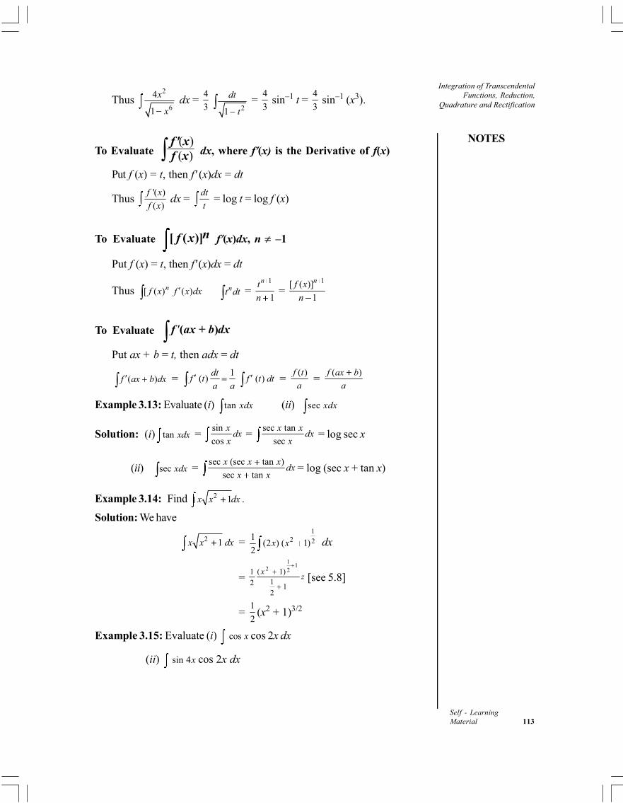
NOTES
Integration of TranscendentalFunctions, Reduction,
Quadrature and Rectification
Self - LearningMaterial 113
Thus 2
6
4
1
x
x dx =
4
3 21
dt
t =
4
3 sin–1 t =
4
3 sin–1 (x3).
To Evaluate ( )( ) f ' x
f x dx, where f(x) is the Derivative of f(x)
Put f (x) = t, then f (x)dx = dt
Thus '( )
( )
f x
f x dx =
dt
t = log t = log f (x)
To Evaluate [ ( )]nf x f(x)dx, n –1
Put f (x) = t, then f (x)dx = dt
Thus [ ( ) ( )nf x f x dx nt dt = 1
1
nt
n =
1[ ( )]
1
nf x
n
To Evaluate ' ( + )f ax b dx
Put ax + b = t, then adx = dt
( )f ax b dx = 1
( )dt
f ta a
( )f t dt = ( )f t
a =
( )f ax b
a
Example 3.13: Evaluate (i) tan xdx (ii) sec xdx
Solution: (i) tan xdx = sin
cos
xdx
x =
sec tan
sec
x xdx
x = log sec x
(ii) sec xdx = sec (sec tan )
sec tan
x x xdx
x x= log (sec x + tan x)
Example 3.14: Find 2 1x x dx .
Solution: We have
2 1x x dx = 1
2 21(2 ) ( 1)
2x x dx
=
11
2 21 ( 1)12 12
xz
[see 5.8]
= 1
2(x2 + 1)3/2
Example 3.15: Evaluate (i) cos x cos 2x dx
(ii) sin 4x cos 2x dx
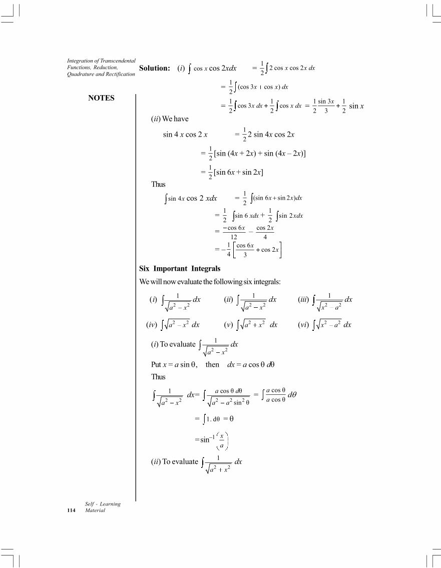
Integration of TranscendentalFunctions, Reduction,Quadrature and Rectification
NOTES
Self - Learning114 Material
Solution: (i) cos x cos 2xdx = 1
2 cos cos 22
x x dx
= 1
(cos 3 cos )2
x x dx
= 1 1
cos 3 cos2 2
x dx x dx = 1 sin 3 1
2 3 2
x sin x
(ii) We have
sin 4 x cos 2 x = 1
22 sin 4x cos 2x
= 1
2[sin (4x + 2x) + sin (4x – 2x)]
= 1
2[sin 6x + sin 2x]
Thus
sin 4x cos 2 xdx = 1
2(sin 6 sin 2 )x x dx
= 1
2 sin 6 xdx +
1
2sin 2xdx
= cos 6
12
x – cos 2
4
x
= –1
4cos 6
cos 23
xx
Six Important Integrals
We will now evaluate the following six integrals:
(i)2 2
1
–a x dx (ii)
2 2
1
a xdx (iii)
2 2
1
x adx
(iv) 2 2a x dx (v) 2 2a x dx (vi) 2 2x a dx
(i) To evaluate 2 2
1
a xdx
Put x = a sin , then dx = a cos d
Thus
2 2
1
a x dx=
2 2 2
cos θ θ
sin θ
a d
a a =
cos θ
cos θ
a
ad
= 1. dθ =
= sin–1 x
a
(ii) To evaluate 2 2
1
a x dx
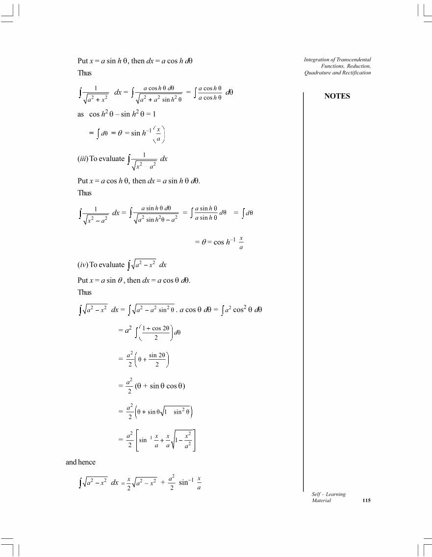
NOTES
Integration of TranscendentalFunctions, Reduction,
Quadrature and Rectification
Self - LearningMaterial 115
Put x = a sin h , then dx = a cos h d
Thus
2 2
1
a x dx =
2 2 2
cos θ θ
sin θ
a h d
a a h = cos θ
cos θ
a h
a h d
as cos h2 – sin h2 = 1
= θd = = sin h–1 x
a
(iii)To evaluate 2 2
1
x a dx
Put x = a cos h then dx = a sin h d.
Thus
2 2
1
x a dx =
2 2 2
sin θ θ
sin θ
a h d
a h a =
sin
sin
a hd
a h = d
= = cos h–1 x
a
(iv)To evaluate 2 2a x dx
Put x = a sin , then dx = a cos dThus
2 2a x dx = 2 2 2sin θa a . a cos d = 2a cos2 d
= a2 1 cos 2θθ
2d
= 2 sin 2θ
θ2 2
a
= 2
2
a ( + sin cos )
= 2
2θ sin θ 1 sin θ2
a
= 2
2
a 21
2sin 1
x x x
a a a
and hence
2 2a x dx 2 2
2
xa x +
2
2
a sin–1 x
a
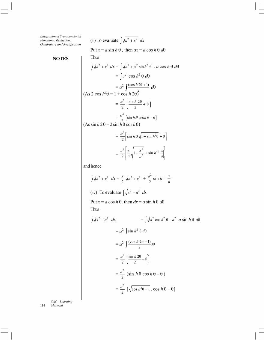
Integration of TranscendentalFunctions, Reduction,Quadrature and Rectification
NOTES
Self - Learning116 Material
(v) To evaluate 2 2a x dx
Put x = a sin h , then dx = a cos h d
Thus
2 2a x dx = 2 2 2sin θa x h . a cos h d
= 2a cos h2 d
= a2 (cos 2θ 1)
2
h d
(As 2 cos h2 = 1 + cos h 2
= 2
2
a sin 2θθ
2
h
= 2
2
a sin cosh h
(As sin h 2 = 2 sin h cos h
= 2
2sin θ 1 sin θ θ2
ah h
= 2 2
12
1 sin2
a x x xh
a aa
and hence
2 2a x dx = 2
x 2 2a x + 2
2
a sin h–1 x
a
(vi) To evaluate 2 2x a dx
Put x = a cos h , then dx = a sin h d
Thus
2 2x a dx = 2 2 2cos θa h a a sin h d
= a2 2sin θ θh d
= a2 (cos 2θ 1)
θ2
hd
= 2
2
a sin 2θθ
2
h
= 2
2
a (sin h cos h – )
= 2
2
a [ 2cos θ 1h . cos h – ]
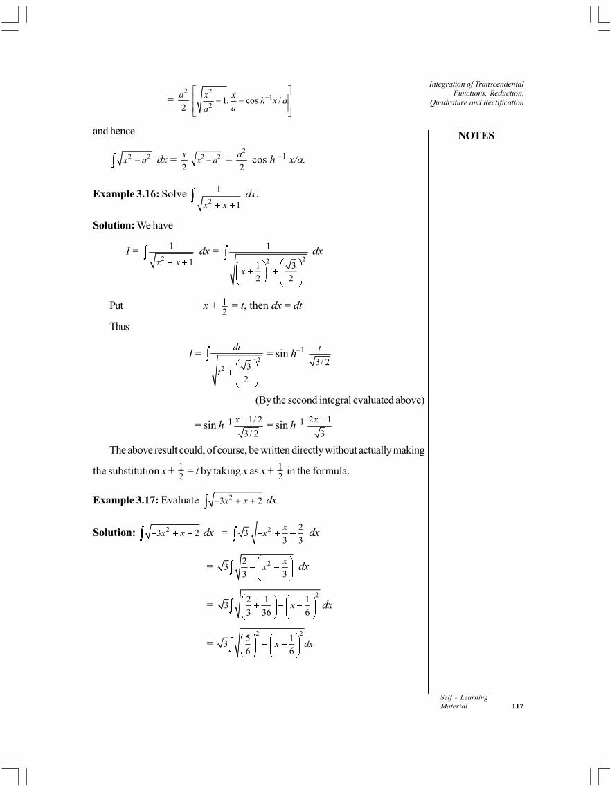
NOTES
Integration of TranscendentalFunctions, Reduction,
Quadrature and Rectification
Self - LearningMaterial 117
= 2
2
a 21
21. cos /
x xh x a
aa
and hence
2 2x a dx = 2
x 2 2x a – 2
2
a cos h –1 x/a.
Example 3.16: Solve 2
1
1x x dx.
Solution: We have
I = 2
1
1x x dx =
22
1
1 3
2 2x
dx
Put x + 12
= t, then dx = dt
Thus
I = 2
2 3
2
dt
t
= sin h–1 3/ 2
t
(By the second integral evaluated above)
= sin h–1 1/ 2
3/ 2
x = sin h–1 2 1
3
x
The above result could, of course, be written directly without actually making
the substitution x + 12 = t by taking x as x + 1
2 in the formula.
Example 3.17: Evaluate 23 2x x dx.
Solution: 23 2x x dx = 2 23
3 3
xx dx
= 223
3 3
xx dx
= 22 1 1
33 36 6
x dx
= 2 2
5 13
6 6x dx
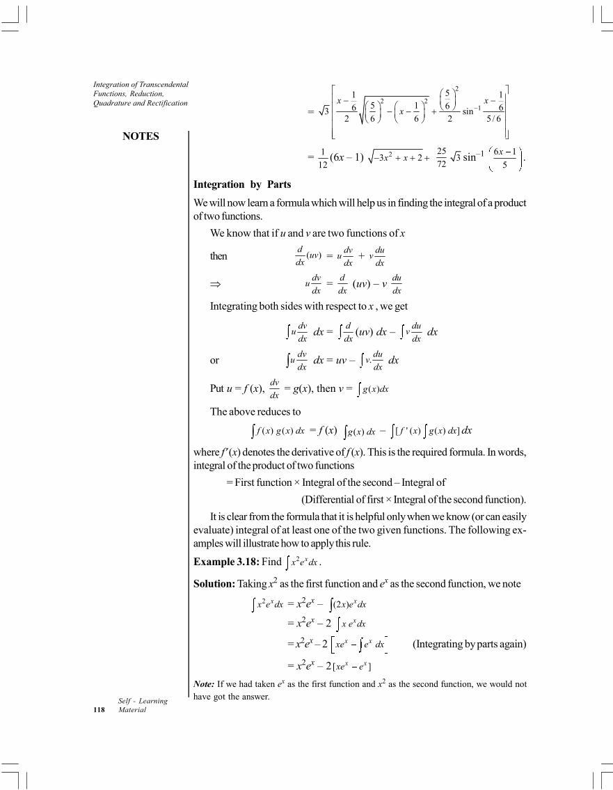
Integration of TranscendentalFunctions, Reduction,Quadrature and Rectification
NOTES
Self - Learning118 Material
=
2
2 21
51 15 1 66 63 sin
2 6 6 2 5 / 6
x xx
= 1
12(6x – 1) 23 2x x
25
723 sin–1 6 1
5
x .
Integration by Parts
We will now learn a formula which will help us in finding the integral of a productof two functions.
We know that if u and v are two functions of x
then ( )d
uvdx
= dv
udx
+ du
vdx
dvu
dx=
d
dx (uv) – v
du
dx
Integrating both sides with respect to x , we get
dvu
dx dx =
d
dx(uv) dx –
duv
dx dx
ordv
udx dx = uv – .
duv
dx dx
Put u = f (x), dv
dx = g(x), then v = ( )g x dx
The above reduces to
( ) ( )f x g x dx = f (x) ( )g x dx – [ ' ( ) ( ) ]f x g x dx dx
where f (x) denotes the derivative of f (x). This is the required formula. In words,integral of the product of two functions
= First function × Integral of the second – Integral of
(Differential of first × Integral of the second function).
It is clear from the formula that it is helpful only when we know (or can easilyevaluate) integral of at least one of the two given functions. The following ex-amples will illustrate how to apply this rule.
Example 3.18: Find 2 xx e dx .
Solution: Taking x2 as the first function and ex as the second function, we note
2 xx e dx = x2ex – (2 ) xx e dx= x2ex – 2 xx e dx
= x2ex – 2 x xxe e dx (Integrating by parts again)
= x2ex – 2 [ ]x xxe e
Note: If we had taken ex as the first function and x2 as the second function, we would nothave got the answer.
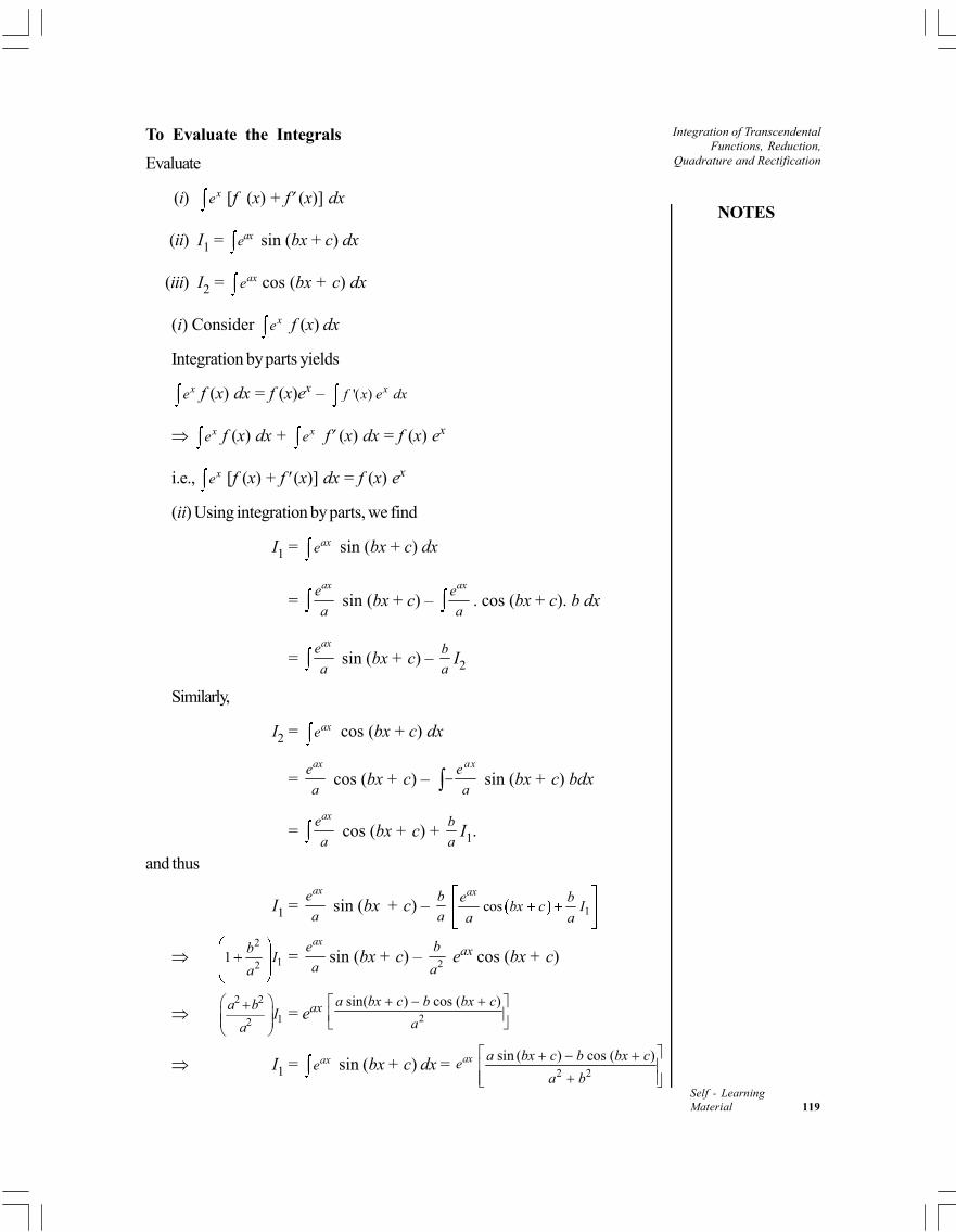
NOTES
Integration of TranscendentalFunctions, Reduction,
Quadrature and Rectification
Self - LearningMaterial 119
To Evaluate the Integrals
Evaluate
(i) xe [f (x) + f (x)] dx
(ii) I1 = axe sin (bx + c) dx
(iii) I2 = axe cos (bx + c) dx
(i) Consider xe f (x) dx
Integration by parts yields
xe f (x) dx = f (x)ex – '( ) xf x e dx
xe f (x) dx + xe f (x) dx = f (x) ex
i.e., xe [f (x) + f (x)] dx = f (x) ex
(ii) Using integration by parts, we find
I1 = axe sin (bx + c) dx
= axe
a sin (bx + c) –
axe
a. cos (bx + c). b dx
= axe
a sin (bx + c) –
b
aI2
Similarly,
I2 = axe cos (bx + c) dx
= axe
a cos (bx + c) –
axe
a sin (bx + c) bdx
= axe
a cos (bx + c) +
b
aI1.
and thus
I1 = axe
a sin (bx + c) –
b
a 1cosaxe b
bx c Ia a
2
121
bI
a=
axe
asin (bx + c) – 2
b
a eax cos (bx + c)
2 2
12
a bI
a
= eax 2
sin( ) cos ( )a bx c b bx c
a
I1 = axe sin (bx + c) dx = axe2 2
sin ( ) cos ( )a bx c b bx c
a b
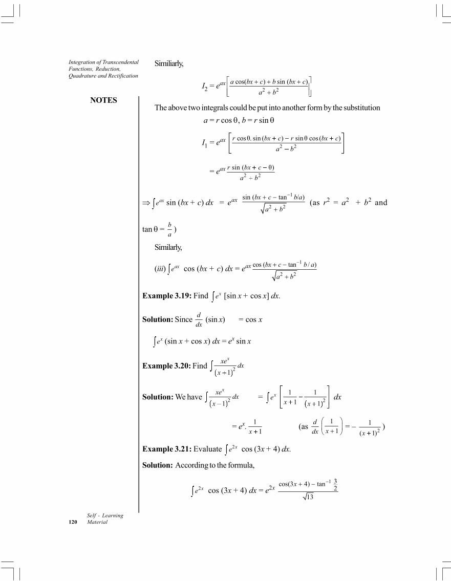
Integration of TranscendentalFunctions, Reduction,Quadrature and Rectification
NOTES
Self - Learning120 Material
Similiarly,
I2 = eax2 2
cos( ) sin ( )a bx c b bx c
a b
The above two integrals could be put into another form by the substitution
a = r cos , b = r sin
I1 = eax 2 2
cosθ. sin ( ) sin θ cos ( )r bx c r bx c
a b
= eax2 2
sin ( θ)r bx c
a b
axe sin (bx + c) dx = eax 1
2 2
sin ( tan / )bx c b a
a b
(as r2 = a2 + b2 and
tan = b
a)
Similarly,
(iii) axe cos (bx + c) dx = eax1
2 2
cos ( tan / )bx c b a
a b
Example 3.19: Find xe [sin x + cos x] dx.
Solution: Since d
dx (sin x) = cos x
xe (sin x + cos x) dx = ex sin x
Example 3.20: Find 21
xxedx
x
Solution: We have 21
xxedx
x= xe 2
1 1
1 1x x dx
= ex.1
1x (as
d
dx
1
1x
= – 2
1
( 1)x)
Example 3.21: Evaluate 2xe cos (3x + 4) dx.
Solution: According to the formula,
2xe cos (3x + 4) dx = e2x 1 3cos(3 4) tan
213
x
NOTES
Integration of TranscendentalFunctions, Reduction,
Quadrature and Rectification
Self - LearningMaterial 121
Some More Examples
We give below a few more examples, where both substitution and integration byparts are used.
Example 3.22: Find 1tan
2 3 / 2(1 )
m xe
x
dx
Solution: Put tan–1 x = t, then x = tan t
Also 2
1
1dx
x = dt and 1 + x2 = 1 + tan2 t = sec2 t
Thus
1tan
2 3 / 2(1 )
m xe
x
dx = sec
mtedt
t = cosmte t dt
= emt
1
2
1cos tan
1
tm
m
where t = tan–1 x
Example 3.23: Evaluate 2 1sinx x dx .
Solution: We have, by integration by parts,
2 1sinx xdx = (sin–1 x) 3
3
x –
3
2
1.
3 1
xdx
x
= 3
3
xsin–1 x – 1
3
3
21
xdx
x. . . .(1)
To evaluate 3
21
xdx
x, put 21 x = t
1 – x2 = t2
–2x dx = 2t dt
x dx = – t dt
Also x2 = 1 – t2
Thus3
21
x dx
x= –
2(1 )t tdt
t = 2( 1)t dt =
3
3
t – t
= 2 3/ 2
2(1 )1
3
xx
Hence the required value is [from Equation (1)]
2 1sinx xdx = 3
3
x sin–1 x – 1
3
2 3/ 22(1 )
13
xx
Integration of TranscendentalFunctions, Reduction,Quadrature and Rectification
NOTES
Self - Learning122 Material
Some More Methods
If the integrand consists of even powers of x only, then the substitution x2 = t, ishelpful while resolving into partial fractions.
Note: The substitution is not to be made in the integral.
Example 3.24: Evaluate 2
2 2( 1)(3 1)
x dx
x x
Solution: Put x2 = t in 2
2 2( 1)(3 1)
x
x x
Then( 1)(3 1)
t
t t
1 3 1
A B
t t
t A (3t + 1) + B (t + 1)
Putting t = – 1 and – 13
, we get
A = 12
, B = – 12
( 1)(3 1)
t
t t=
1
2( 1)t –
1
2(3 1)t
Thus2
2 2( 1)(3 1)
x
x x=
2
1
2( 1)x –
2
1
2(3 1)x
2
2 2( 1)(3 1)
x
x x dx = 1
2
2 1
dx
x –
212 3 1
dx
x
= 12
tan–1 x – 2
16 1
3
dx
x
= 12
tan–1 x – 1 1.
6 1/ 3 tan–1
1/ 3
x
= 12
tan–1 x – 2 3
x tan–1 ( 3)x
We give two more examples that would help us in solving many other prob-lems.
Example 3.25: Solve 2
4
1
1
xdx
x
Solution: We have I = 2
4
1
1
xdx
x =
2
2 2
1 1/
1/
xdx
x x
Put x – 1
x= t
Then 2
11
x dx = dt
NOTES
Integration of TranscendentalFunctions, Reduction,
Quadrature and Rectification
Self - LearningMaterial 123
Also x2 + 2
1
x – 2 = t2
So I = 2 2
dt
t =
2
t tan–1 2
t = 1
2 tan–1 1 1
2x
x
Substitution before Resolving into Partial Fractions
The integration process is sometimes greatly simplified by a substitution as is seenin the following examples:
Example 3.26: Solve 4( 1)
dx
x x
Solution: Put x4 = t, then 4x3 dx = dt
Thus4( 1)
dx
x xdt =
3
4 4( 1)
x dx
x xdt = 1
4
( 1)
dt
t t
Now1
( 1)t t =
1
1t –
1
t
and hence the given integral
= 1 114 1t t
dt = 14
[log (t – 1) – log t]
= 14 log 1t
t
= 14 log
4
4
1x
x
Example 3.27: Solve π/4
0
tan x dx
Solution: Put tan x = t, then tan x = t2
and sec2 x dx = 2 t dt
dx = 2
2
1 tan
t
x dt =
4
2
1
t dt
t
Also when x = 0, t = tan 0 = 0
when x = π
4, t = π
tan 14
Hence the given integral becomes
1
40
.2
1
t t dt
t= 2
1 2
40 1
t
t
= 12 2
12
0
2 2 1 112 log 2 tan48 22 1
t t t
tt t
Integration of TranscendentalFunctions, Reduction,Quadrature and Rectification
NOTES
Self - Learning124 Material
By integrating,
= 1 12 2 2 2 2 22 log tan 0 log 1 tan
8 4 8 42 2
= 2 2 2 22 log
8 4 22 2
= 2
4 log
2 2 2
42 2 = 1
2 2 log
2 2 1
2 2 2 2
Integrals of the Type cos + sin
dx
a + b x c x, b2 + c2 0
The substitution tan 2
x = t, converts every rational function of sin x and cos x into
a rational function of t and we can then evaluate the integral by using the previousmethods.
Example 3.28: Evaluate (i) π/2
20 4 5 cos
dx
x(ii)
π
05 3 cos
dx
x
Solution: (i) Put tan 2
x = t, then 12
sec2 2
x dx = dt
dx = 2
2
1 tan / 2
dt
x =
2
2
1
dt
t
Also as cos x = 2
2
1 tan / 2
1 tan / 2
x
x =
2
2
1
1
t
t
the given integral reduces to
1
220
2
2
5 5(1 ) 4
1
dt
tt
t
Note, when = 0
tan 0 0
When π / 2
tan π/4 1
x
t
x
t
= 21
2 20 4 4 5 5
dt
t t = 2
1
20 9
dt
t
= 2. 1
0
1 3log
2 3 3
t
t
= 13
log 13
3 1
3 1 log
3
3
= 13
log 2
NOTES
Integration of TranscendentalFunctions, Reduction,
Quadrature and Rectification
Self - LearningMaterial 125
(ii) Put tan 2
x = t, then 12
sec2 2
x dx = dt
dx = 2
2
1 tan / 2
dt
x =
2
2
1
dt
t
Also as cos x = 2
2
1 tan / 2
1 tan / 2
x
x =
2
2
1
1
t
t
the given integral reduces to
220
2
2
(1 )(1 ) 5 3
1
dt
tt
t
Note, when 0, tan 0 0
πWhen π, tan
2
x t
x t
= 2 20
25 5 3 3
dt
t t = 2
0
22 8
dt
t = 2
0 4
dt
t
= 112
0
tan2
t = 12 tan–1 – 1
2 tan–1 0
= π π0
2 2
Example 3.29: Evaluate 23 2 cos
dx
x.
Solution: Put tan x = t, then sec2 x dx = dt
Now23 2 cos
dx
x=
2
2
sec
3 sec 2
x dx
x =
23(1 ) 2
dt
t
= 23 5
dt
t =
213 5
3
dt
t
= 13 × 3
5 tan–1 3
5
t
= 1
15tan–1 3
tan5
x
Integration of cos sincos sin
a x + b xc x + d x
, (a2 + b2) (c2 + d2) 0
We determine two constants and such that,
a cos x + b sin x = (–c sin x + d cos x) + (c cos x + d sin x)
where – c sin x + d cos x = d
dx(c cos x + d sin x)
Integration of TranscendentalFunctions, Reduction,Quadrature and Rectification
NOTES
Self - Learning126 Material
Comparing coefficients of cos x and sin x, we get
a = d + c
b = – c + d
= 2 2
ad bc
d c, =
2 2
ac bd
d c
Hence
cos sin
cos sin
a x b x
c x d x dx =
sin cosμ 1.
cos sin
c x d xdx dx
c x d x
= log (c cos x + d sin x) + x
Integration of cos sincos sin
a x + b x + cd x+ e x + f
In this case we determine three constants , , , such that a cos x+b sin x+c= (d cos x + e sin x + f) + (–d sin x + e cos x) + v and proceed as in the earliercase.
Example 3.30: Find 4 sin + 2 cos + 3
2 sin + cos + 3
x x
x x dx
Solution: We determine , , such that,
4 sin x + 2 cos x + 3 = (2 sin x + cos x + 3) + (2 cos x – sin x) + Comparing coefficients of sin x, cos x and the constant terms, we get
4 = 2 – ,2 = + 2 3 = 3 +
= 2, = 0, = –3
Thus
4 sin x + 2 cos x + 3 = 2(2 sin x + cos x + 3) + 0 (2 cos x – 1) – 3
4 sin 2 cos 3
2 sin cos 3
x x
x x
dx= 2
11. 3
2 sin cos 3dx
x x dx
= 2x – 31
2 sin cos 3x x dx
Example 3.31: To solve 1
2 sin cos 3x xdx
Solution: We put tan 2
x = t, then dx = 2
2
1
dt
t
and the integral
= 2
22 2
2
2.2 1(1 ) 3
1 1
dt
t tt
t t
NOTES
Integration of TranscendentalFunctions, Reduction,
Quadrature and Rectification
Self - LearningMaterial 127
= 2 2
2
4 1 3 3
dt
t t t
= 2 2 2
dt
t t
= 2( 1) 1
dt
t
= tan–1 (t + 1) = tan–1 1 tan2
x
Hence the required result is
2x – 3 tan–1 1 tan2
x
Check Your Progress
1. Define the terms integration and integrand.
2. Integrate the following functions with respect to x:
(a) (i)1x
(ii) 3/ 2
1
x(iii) (1 )x x (iv)
3
2
ax bx
(b) (i) e2x (ii) e2x – 3 (iii) 1xe
(c) Integrate the following functions:
(i)1
2
sin
1
x
x
(ii) cos (log )x
x
(iii) 1x xe e
3. Integrate the following functions:
(a) (i)2
1
2 2x x (ii) 2
1
1 12 9x x (iii)2 2
1
2 / 2a x
(b) (i) 22 3 4x x (ii) 22 3x (iii) 29 4x
3.3 REDUCTION FORMULA
A formula which connects an integral with another integral, having the same formas the given integral but of lower degree or order and easier to integrate is calleda reduction formula.
A reduction formula is usually obtained by the method of integration byparts and is used to integrate by successive reduction.
Integration of TranscendentalFunctions, Reduction,Quadrature and Rectification
NOTES
Self - Learning128 Material
Reduction Formulae for sinn x dx And cosn x dx
Let In = sinn x dx.
For applying the method of integration by parts, we write
sinnx = sinn1x.sin x
In
= sinn1 x sin x dx
= sinn1 x ( cos x) 1sin ( cos )ndx x dx
dx
= sinn1 x.cos x + 2( 1)sin .cos .cosnn x x x dx= 1 2 2sin .cos ( 1) sin .(1 sin )n nx x n x x dx = 1 2sin .cos ( 1) sin ( 1) sinn n nx x n xdx n x dx = 1 2sin cos ( 1) sin ( 1)In n
nx x n xdx n By transposing the last term to the left, we get
1 2I sin cos ( 1) sinn nnn x x n xdx
Hence, 1
2sin .cos ( 1)sin sin
nn nx x n
xdx xdxn n
…(1)
which is the required reduction formula.
If In = sinn x dx, then I
n
2 = sinn2 x dx
Equation (1) can also be written as
1
2
sin cos ( 1)I I
n
n n
x x n
n n
Similarly, we can get the reduction formula for cosn xdx as
1
2cos sin ( 1)cos cos
nn nx x n
xdx xdxn n
… (2)
which is the required reduction formula.
3.3.1 Walli’s Formula
To evaluate / 2
0sinn xdx
and/ 2
0cosn xdx
where ‘n’ is a natural number..
From the reduction formula of sinn xdx , we have
1
2sin .cos ( 1)sin sin
nn nx x n
xdx xdxn n
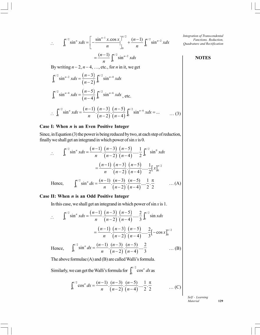
NOTES
Integration of TranscendentalFunctions, Reduction,
Quadrature and Rectification
Self - LearningMaterial 129
/ 21/ 2 / 2 2
0 00
sin .cos ( 1)sin sin
nn nx x n
xdx xdxn n
/ 2 2
0
( 1)sinnn
xdxn
By writing n 2, n 4, …, etc., for n in it, we get
/ 2 / 22 4
0 0
3sin sin
2n nn
xdx xdxn
/ 2 / 24 6
0 0
5sin sin
4n nn
xdx xdxn
, etc.
/ 2 / 2 6
0 0
1 3 5sin . . sin ...
2 4n nn n n
xdx xdxn n n
… (3)
Case I: When n is an Even Positive Integer
Since, in Equation (3) the power is being reduced by two, at each step of reduction,finally we shall get an integrand in which power of sin x is 0.
/ 2 / 2 0
0 0
1 3 5 1sin . . ..... sin
2 4 2n n n n
xdx xdxn n n
/ 2
0
1 3 5 1. . .....
2 4 2
n n nx
n n n
Hence,
/ 2
0
( 1) ( 3) ( 5) 1sin . . .... .
2 4 2 2n n n n
dxn n n
… (A)
Case II: When n is an Odd Positive Integer
In this case, we shall get an integrand in which power of sin x is 1.
/ 2 / 2
0 0
1 3 5 2sin . . ..... sin
2 4 3n n n n
xdx xdxn n n
/ 2
0
1 3 5 2. . ..... cos
2 4 3
n n nx
n n n
Hence, / 2
0
( 1) ( 3) ( 5) 2sin . . ....
2 4 3n n n n
dxn n n
… (B)
The above formulae (A) and (B) are called Walli’s formula.
Similarly, we can get the Walli’s formula for / 2
0cosn dx
as
/ 2
0
( 1) ( 3) ( 5) 1cos . . .... .
2 4 2 2n n n n
dxn n n
… (C)
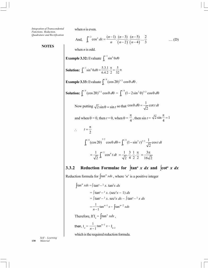
Integration of TranscendentalFunctions, Reduction,Quadrature and Rectification
NOTES
Self - Learning130 Material
when n is even.
And, / 2
0
( 1) ( 3) ( 5) 2cos . . ....
2 4 3n n n n
dxn n n
… (D)
when n is odd.
Example 3.32: Evaluate / 2 6
0sin d
Solution: / 2 6
0sin d
=
5.3.1 5.
6.4.2 2 32
Example 3.33: Evaluate/ 4 3/ 2
0(cos 2 ) cos d
.
Solution:/ 4 3/ 2
0(cos 2 ) cos d
=
/ 4 2 3/ 2
0(1 2sin ) cos d
Now putting 2 sin sin t so that 1
cos cot2
d t dt
and when = 0, then t = 0, when = 4
, then sin t = 2 sin 1
4
2
t
3/ 2/ 4 / 4 2 3/ 2
0 0
1(cos 2 ) cos (1 sin ) cos
2d t t dt
/ 2 4
0
1cos
2t dt
1 3 1. . .4 2 22
16 2
3.3.2 Reduction Formulae for tann x dx and cotn x dx
Reduction formula for tann xdx , where ‘n’ is a positive integer
tann xdx = tann 2 x. tan2x dx
= tann 2 x. (sec2x 1) dx
= tann 2 x. sec2x dx tann 2 x dx
= 1 21tan tan
1n nx xdx
n
Therefore, If In = tann xdx ,
then, In = 11
tan1
n xn
In–2
which is the required reduction formula.
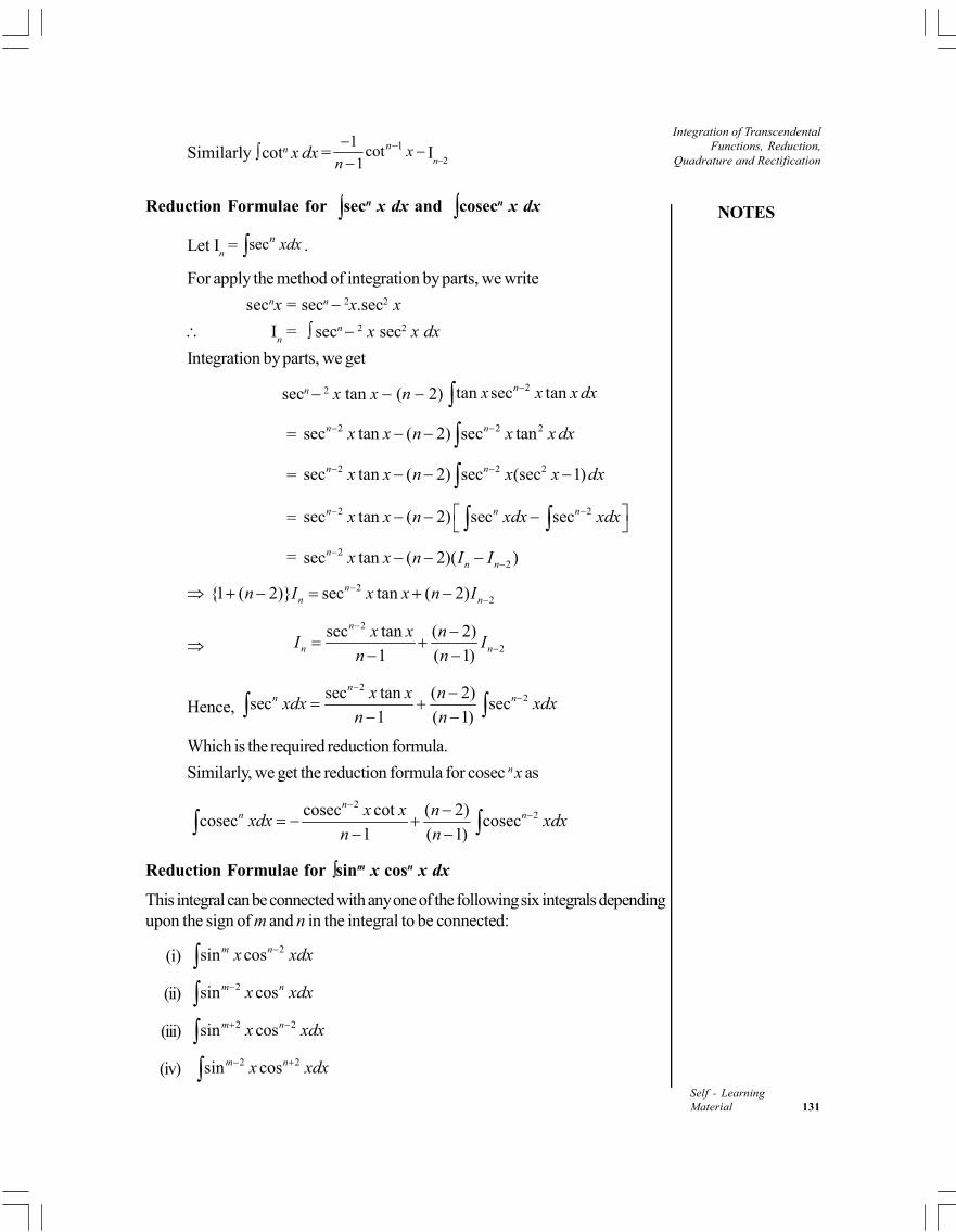
NOTES
Integration of TranscendentalFunctions, Reduction,
Quadrature and Rectification
Self - LearningMaterial 131
Similarly cotn x dx = 11cot
1n x
n
In–2
Reduction Formulae for secn x dx and cosecn x dx
Let In = secn xdx .
For apply the method of integration by parts, we write
secnx = secn 2x.sec2 x
In
= secn 2 x sec2 x dx
Integration by parts, we get
secn 2 x tan x (n 2) 2tan sec tannx x x dx= 2 2 2sec tan ( 2) sec tann nx x n x x dx = 2 2 2sec tan ( 2) sec (sec 1)n nx x n x x dx = 2 2sec tan ( 2) sec secn n nx x n xdx xdx = 2
2sec tan ( 2)( )nn nx x n I I
22{1 ( 2)} sec tan ( 2)n
n nn I x x n I
2
2
sec tan ( 2)
1 ( 1)
n
n n
x x nI I
n n
Hence, 2
2sec tan ( 2)sec sec
1 ( 1)
nn nx x n
xdx xdxn n
Which is the required reduction formula.
Similarly, we get the reduction formula for cosec n x as
22cosec cot ( 2)
cosec cosec1 ( 1)
nn nx x n
xdx xdxn n
Reduction Formulae for sinm x cosn x dx
This integral can be connected with any one of the following six integrals dependingupon the sign of m and n in the integral to be connected:
(i) 2sin cosm nx xdx(ii) 2sin cosm nx xdx(iii) 2 2sin cosm nx xdx (iv) 2 2sin cosm nx xdx
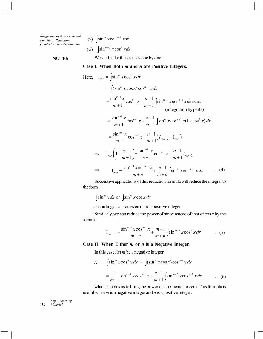
Integration of TranscendentalFunctions, Reduction,Quadrature and Rectification
NOTES
Self - Learning132 Material
(v) 2sin cosm nx xdx(vi) 2sin cosm nx xdx
We shall take these cases one by one.
Case I: When Both m and n are Positive Integers.
Here, ,I sin cosm nm n x x dx
1(sin cos ) cosm nx x x dx
1
1 1 2sin 1cos sin cos sin
1 1
mn m nx n
x x x x dxm m
(integration by parts)
1
1 2 2sin 1cos sin cos (1 cos )
1 1
mn m nx n
x x x x dxm m
1
1, 2 ,
sin 1cos I
1 1
mn
m n m n
x nx I
m m
1
1, , 2
1 sin 1I 1 cos
1 1 1
mn
m n m n
n x nx I
m m m
1 1
2,
sin cos 1I sin cos
m nm n
m n
x x nx x dx
m n m n
… (4)
Successive applications of this reduction formula will reduce the integral tothe form
sin or sin cosm mx dx x x dx according as n is an even or odd positive integer.
Similarly, we can reduce the power of sin x instead of that of cos x by theformula
1 12
,
sin cos 1I sin cos
m nm n
m n
x x mx x dx
m n m n
…(5)
Case II: When Either m or n is a Negative Integer.
In this case, let m be a negative integer.
sin cosm nx x dx = 1(sin cos ) cosm nx x x dx1 1 2 21 1
sin cos sin cos1 1
m n m nnx x x x dx
m m
… (6)
which enables us to bring the power of sin x nearer to zero. This formula isuseful when m is a negative integer and n is a positive integer.
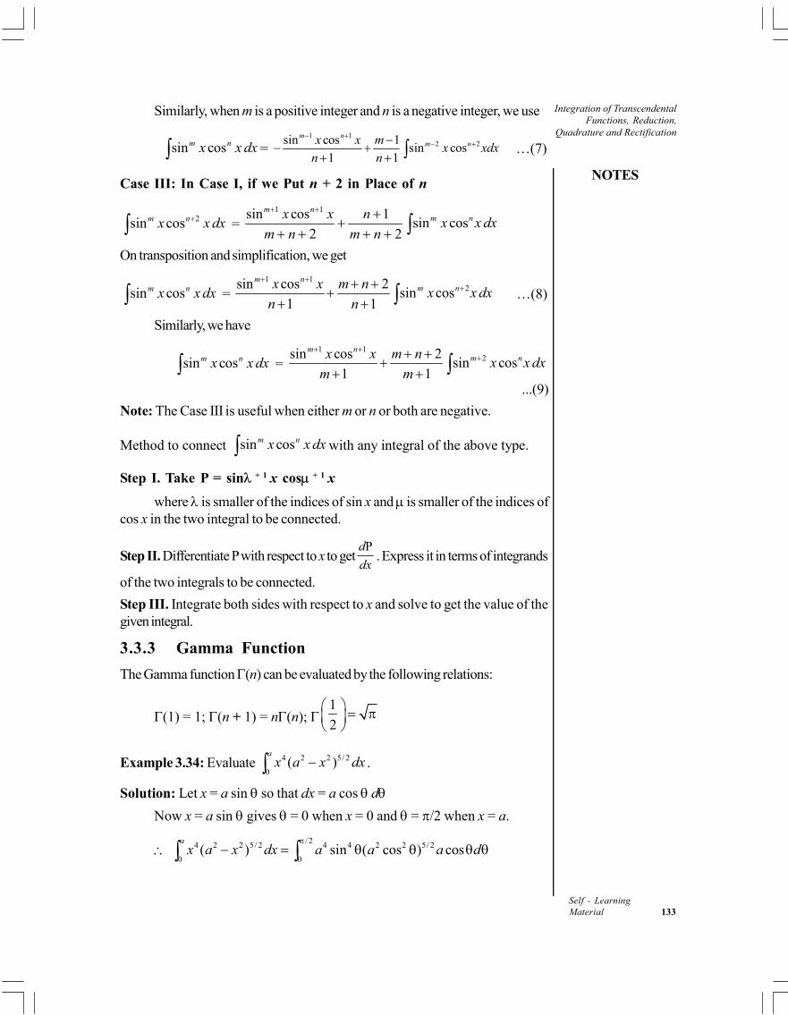
NOTES
Integration of TranscendentalFunctions, Reduction,
Quadrature and Rectification
Self - LearningMaterial 133
Similarly, when m is a positive integer and n is a negative integer, we use
sin cosm nx x dx = 1 1
2 2sin cos 1sin cos
1 1
m nm nx x m
x xdxn n
…(7)
Case III: In Case I, if we Put n + 2 in Place of n
2sin cosm nx x dx = 1 1sin cos 1
sin cos2 2
m nm nx x n
x x dxm n m n
On transposition and simplification, we get
sin cosm nx x dx = 1 1
2sin cos 2sin cos
1 1
m nm nx x m n
x x dxn n
…(8)
Similarly, we have
sin cosm nx x dx = 1 1
2sin cos 2sin cos
1 1
m nm nx x m n
x x dxm m
...(9)
Note: The Case III is useful when either m or n or both are negative.
Method to connect sin cosm nx x dx with any integral of the above type.
Step I. Take P = sin + 1 x cos + 1 x
where is smaller of the indices of sin x and is smaller of the indices ofcos x in the two integral to be connected.
Step II. Differentiate P with respect to x to getPd
dx. Express it in terms of integrands
of the two integrals to be connected.
Step III. Integrate both sides with respect to x and solve to get the value of thegiven integral.
3.3.3 Gamma Function
The Gamma function (n) can be evaluated by the following relations:
(1) = 1; (n + 1) = n(n); 1
2
Example 3.34: Evaluate 4 2 2 5/ 2
0( )
ax a x dx .
Solution: Let x = a sin so that dx = a cos d
Now x = a sin gives = 0 when x = 0 and = /2 when x = a.
/ 24 2 2 5/ 2 4 4 2 2 5/ 2
0 0( ) sin ( cos ) cos
ax a x dx a a a d
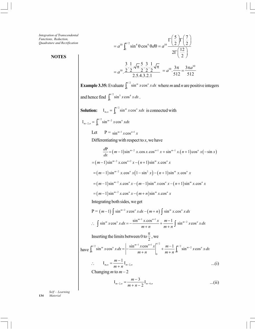
Integration of TranscendentalFunctions, Reduction,Quadrature and Rectification
NOTES
Self - Learning134 Material
/ 210 4 6 10
0
5 72 2
sin cos12
22
a d a
10
3 1 5 3 1. . . .
2 2 2 2 2.2.5.4.3.2.1
a
10
10.512 512
aa
Example 3.35: Evaluate/ 2
0sin cosm nx x dx
where m and n are positive integers
and hence find / 2 5 4
0sin cosx x dx
.
Solution:/ 2
m, 0I sin cosm n
n x xdx
is connected with
/ 2 2
m 2, 0I sin cosm n
n x xdx
Let P = 1 1sin cosm nx x
Differentiating with respect to x, we have
2 1 1P1 sin .cos .cos sin . 1 cos sinm n m nd
m x x x x n x xdx
2 21 sin .cos 1 sin .cosm n m nm x x n x x
2 21 sin .cos 1 sin 1 sin .cosm n m nm x x x n x x
21 sin .cos 1 sin cos 1 sin .cosm n m n m nm x x m x x n x x
21 sin .cos sin .cosm n m nm x x m n x x
Integrating both sides, we get
P = 21 sin cos sin .cosm n m nm x x dx m n x x dx
1 1
2sin .cos 1sin cos sin cos
m nm n m nx x m
x x dx x x dxm n m n
Inserting the limits between 0 to2
, we
have
/ 21 1/ 2 / 2 2
0 00
sin cos 1sin cos sin cos
m nm n m nx x m
x x dx x x dxm n m n
m, 2,
1I In m n
m
m n
...(i)
Changing m to m – 2
m 2, 4,
3I I
2n m n
m
m n
...(ii)
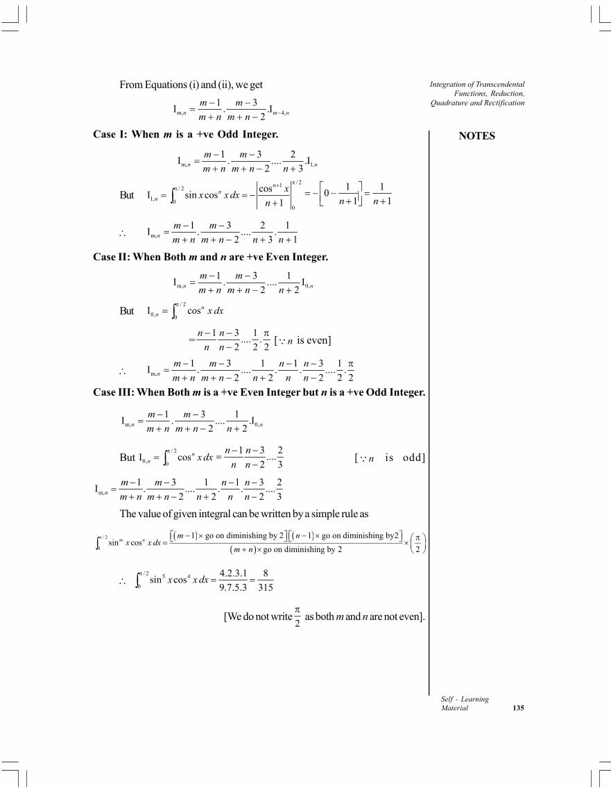
NOTES
Integration of TranscendentalFunctions, Reduction,
Quadrature and Rectification
Self - LearningMaterial 135
From Equations (i) and (ii), we get
m, 4,
1 3I . .I
2n m n
m m
m n m n
Case I: When m is a +ve Odd Integer.
m, 1,
1 3 2I . .... .I
2 3n n
m m
m n m n n
But/ 21
/ 2
1, 00
cosI sin cos
1
nn
n
xx x dx
n
1 1
01 1n n
m,
1 3 2 1I . .... .
2 3 1n
m m
m n m n n n
Case II: When Both m and n are +ve Even Integer.
m, 0,
1 3 1I . .... I
2 2n n
m m
m n m n n
But/ 2
0, 0I cosn
n x dx
=1 3 1
.... .2 2 2
n n
n n
[ n is even]
m,
1 3 1 1 3 1I . .... . . .... .
2 2 2 2 2n
m m n n
m n m n n n n
Case III: When Both m is a +ve Even Integer but n is a +ve Odd Integer.
m, 0,
1 3 1I . .... .I
2 2n n
m m
m n m n n
But / 2
0, 0I cosn
n x dx
1 3 2
....2 3
n n
n n
[ n is odd]
m,
1 3 1 1 3 2I . .... . . ....
2 2 2 3n
m m n n
m n m n n n n
The value of given integral can be written by a simple rule as
/ 2
0
1 go on diminishing by 2 1 go on diminishing by2sin cos
go on diminishing by 2 2m n
m nx x dx
m n
/ 2 5 4
0
4.2.3.1 8sin cos
9.7.5.3 315x x dx
[We do not write2
as both m and n are not even].
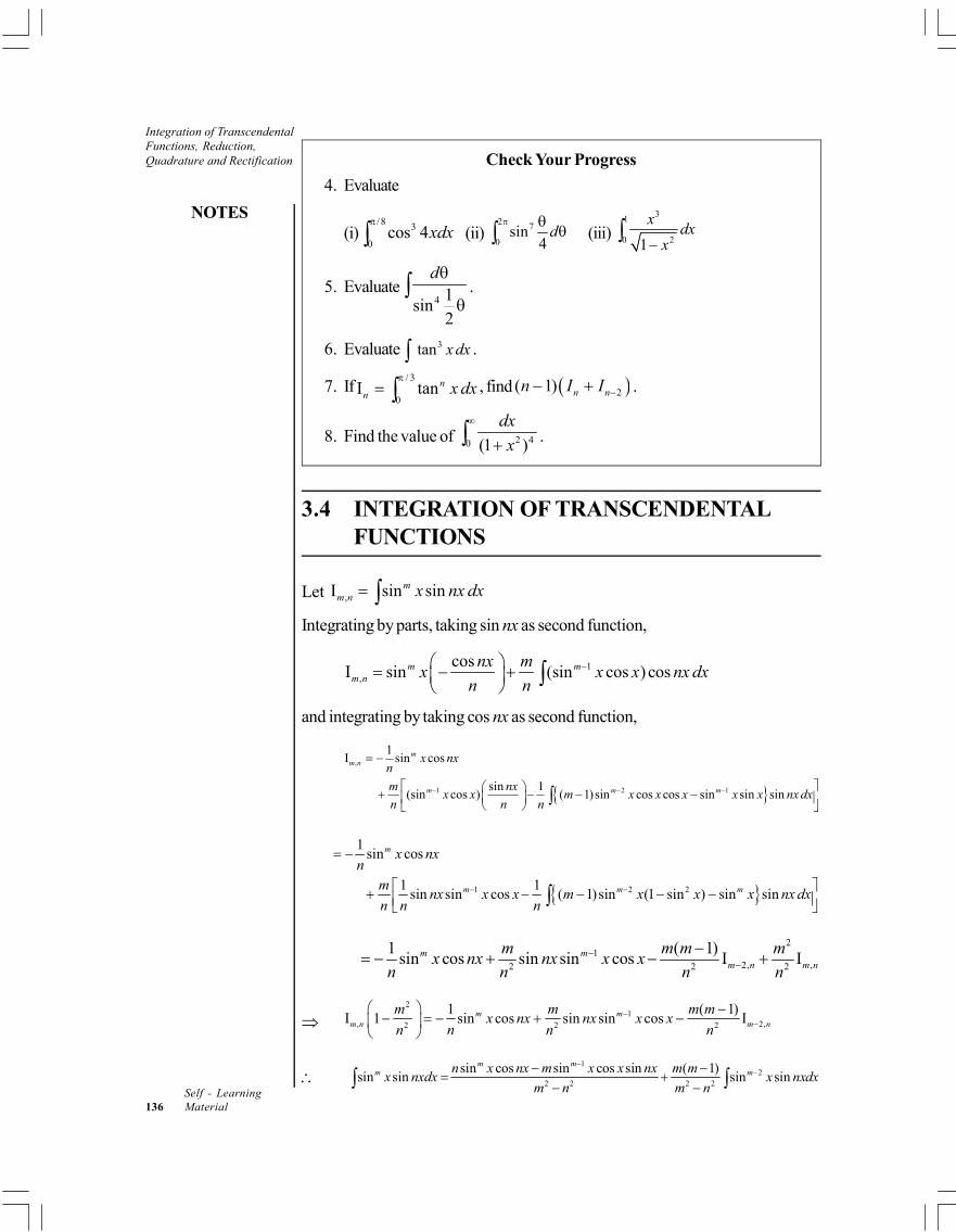
Integration of TranscendentalFunctions, Reduction,Quadrature and Rectification
NOTES
Self - Learning136 Material
Check Your Progress
4. Evaluate
(i)/ 8 3
0cos 4
xdx (ii) 2 7
0sin
4d
(iii)
31
0 21
xdx
x
5. Evaluate4 1
sin2
d
.
6. Evaluate 3tan x dx .
7. If/ 3
0I tann
n x dx
, find 2( 1) n nn I I .
8. Find the value of 2 40 (1 )
dx
x
.
3.4 INTEGRATION OF TRANSCENDENTALFUNCTIONS
Let ,I sin sinmm n x nx dx
Integrating by parts, taking sin nx as second function,
1,
cosI sin (sin cos ) cosm m
m n
nx mx x x nx dx
n n
and integrating by taking cos nx as second function,
,
1 2 1
1I sin cos
sin 1(sin cos ) ( 1)sin cos cos sin sin sin
mm n
m m m
x nxn
m nxx x m x x x x x nx dx
n n n
1 2 2
1sin cos
1 1sin sin cos ( 1)sin (1 sin ) sin sin
m
m m m
x nxn
mnx x x m x x x nx dx
n n n
2
12, ,2 2 2
1 ( 1)sin cos sin sin cos I Im m
m n m n
m m m mx nx nx x x
n n n n
2
1, 2,2 2 2
1 ( 1)I 1 sin cos sin sin cos Im m
m n m n
m m m mx nx nx x x
nn n n
1
22 2 2 2
sin cos sin cos sin ( 1)sin sin sin sin
m mm mn x nx m x x nx m m
x nxdx x nxdxm n m n
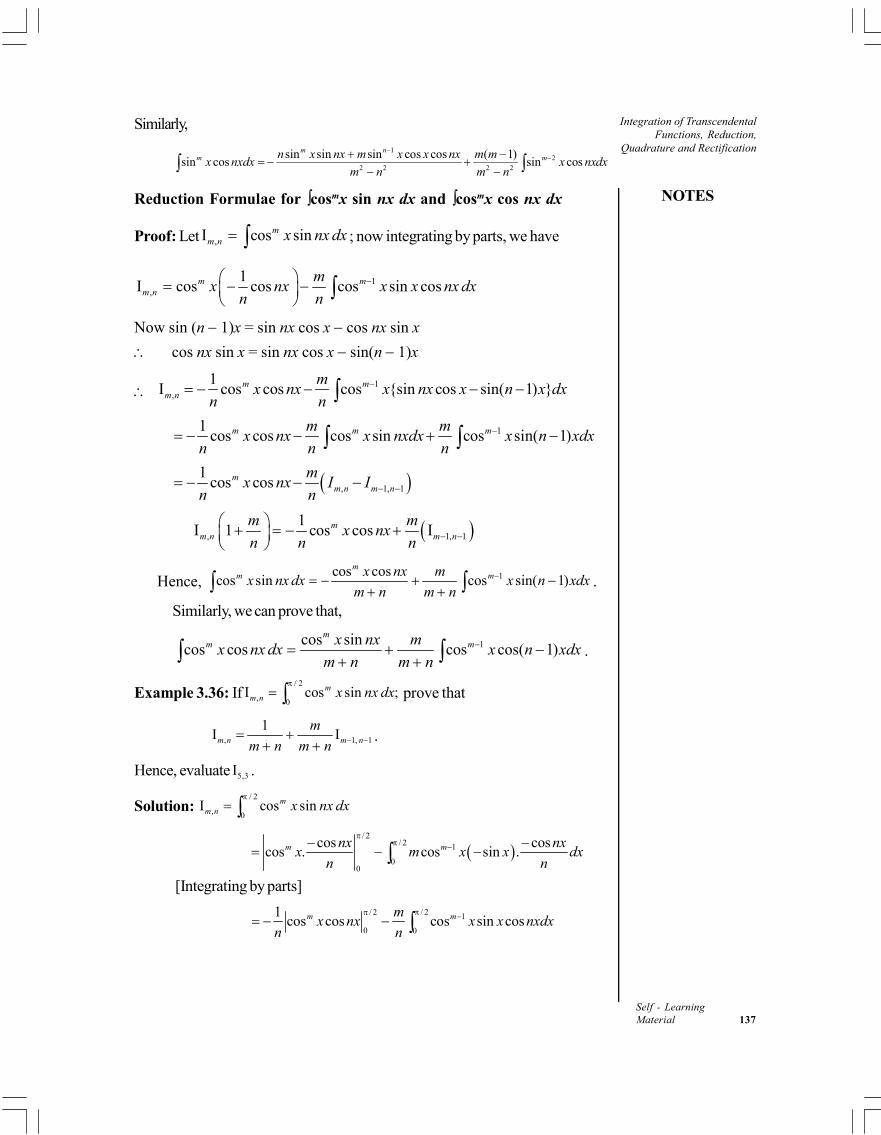
NOTES
Integration of TranscendentalFunctions, Reduction,
Quadrature and Rectification
Self - LearningMaterial 137
Similarly,
12
2 2 2 2
sin sin sin cos cos ( 1)sin cos sin cos
m nm mn x nx m x x nx m m
x nxdx x nxdxm n m n
Reduction Formulae for cosmx sin nx dx and cosmx cos nx dx
Proof: Let ,I cos sinmm n x nx dx ; now integrating by parts, we have
1,
1I cos cos cos sin cosm m
m n
mx nx x x nx dx
n n
Now sin (n 1)x = sin nx cos x cos nx sin x
cos nx sin x = sin nx cos x sin(n 1)x
1
,
1I cos cos cos {sin cos sin( 1) }m m
m n
mx nx x nx x n x dx
n n
11cos cos cos sin cos sin( 1)m m mm m
x nx x nxdx x n xdxn n n
, 1, 1
1cos cosm
m n m n
mx nx I I
n n
, 1, 1
1I 1 cos cos Im
m n m n
m mx nx
n n n
Hence, 1cos coscos sin cos sin( 1)
mm mx nx m
x nx dx x n xdxm n m n
.
Similarly, we can prove that,
1cos sincos cos cos cos( 1)
mm mx nx m
x nx dx x n xdxm n m n
.
Example 3.36: If/ 2
, 0I cos sin ;m
m n x nx dx
prove that
, 1, 1
1I Im n m n
m
m n m n
.
Hence, evaluate 5,3I .
Solution: / 2
, 0I cos sinm
m n x nx dx
/ 2
/ 2 1
00
cos coscos . cos sin .m mnx nx
x m x x dxn n
[Integrating by parts]
/ 2/ 2 1
0 0
1cos cos cos sin cosm mm
x nx x x nxdxn n
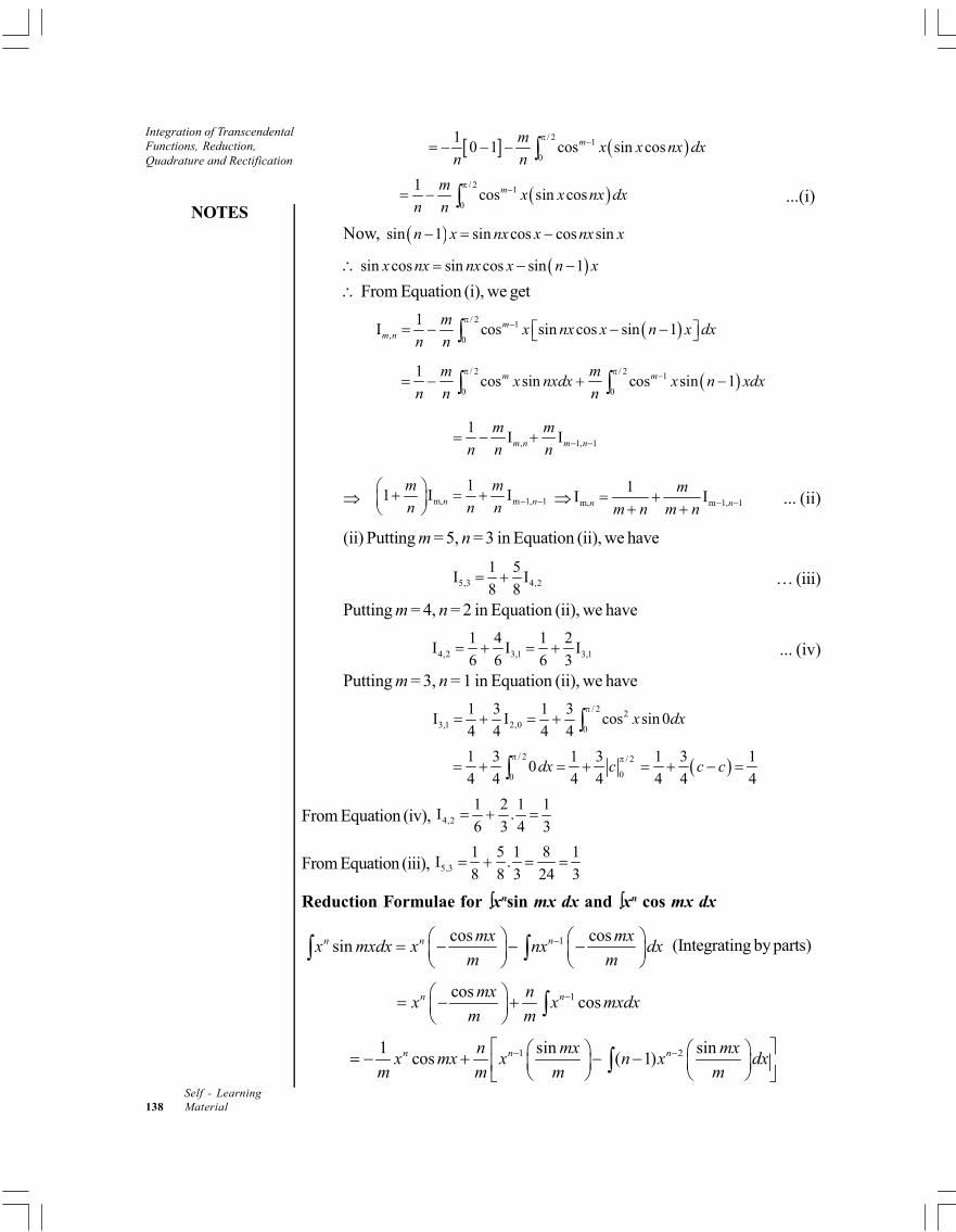
Integration of TranscendentalFunctions, Reduction,Quadrature and Rectification
NOTES
Self - Learning138 Material
/ 2 1
0
10 1 cos sin cosmm
x x nx dxn n
/ 2 1
0
1cos sin cosmm
x x nx dxn n
...(i)
Now, sin 1 sin cos cos sinn x nx x nx x
sin cos sin cos sin 1x nx nx x n x
From Equation (i), we get
/ 2 1
, 0
1I cos sin cos sin 1m
m n
mx nx x n x dx
n n
/ 2 / 2 1
0 0
1cos sin cos sin 1m mm m
x nxdx x n xdxn n n
, 1, 1
1I Im n m n
m m
n n n
m, m 1, 1
11 I In n
m m
n n n
m, m 1, 1
1I In n
m
m n m n
... (ii)
(ii) Putting m = 5, n = 3 in Equation (ii), we have
5,3 4,2
1 5I I
8 8 … (iii)
Putting m = 4, n = 2 in Equation (ii), we have
4,2 3,1 3,1
1 4 1 2I I I
6 6 6 3 ... (iv)
Putting m = 3, n = 1 in Equation (ii), we have
/ 2 2
3,1 2,0 0
1 3 1 3I I cos sin 0
4 4 4 4x dx
/ 2 / 2
00
1 3 1 30
4 4 4 4dx c
1 3 1
4 4 4c c
From Equation (iv), 4,2
1 2 1 1I .
6 3 4 3
From Equation (iii), 5,3
1 5 1 8 1I .
8 8 3 24 3
Reduction Formulae for xnsin mx dx and xn cos mx dx
1cos cossinn n nmx mx
x mxdx x nx dxm m
(Integrating by parts)
1coscosn nmx n
x x mxdxm m
1 21 sin sin
cos ( 1)n n nn mx mxx mx x n x dx
m m m m
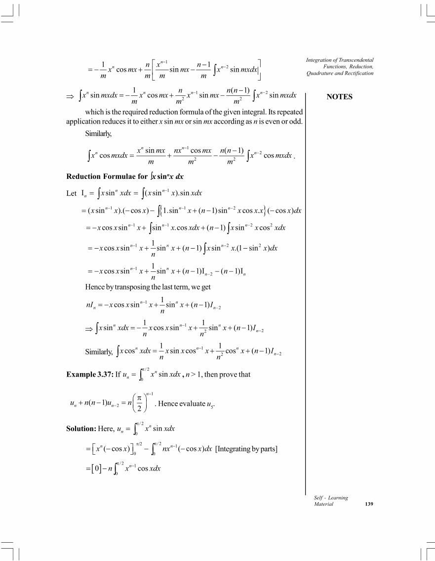
NOTES
Integration of TranscendentalFunctions, Reduction,
Quadrature and Rectification
Self - LearningMaterial 139
1
21 1cos sin sin
nn nn x n
x mx mx x mxdxm m m m
1 2
2 2
1 ( 1)sin cos sin sinn n n nn n n
x mxdx x mx x mx x mxdxm m m
which is the required reduction formula of the given integral. Its repeatedapplication reduces it to either x sin mx or sin mx according as n is even or odd.
Similarly,
12
2 2
sin cos ( 1)cos cos
n nn nx mx nx mx n n
x mxdx x mxdxm m m
.
Reduction Formulae for x sinnx dx
Let I sinnn x xdx 1( sin ).sinnx x xdx 1 1 2( sin ).( cos ) 1.sin ( 1)sin cos . ( cos )n n nx x x x n x x x x dx
1 1 2 2cos sin sin .cos ( 1) sin cosn n nx x x x xdx n x x xdx
1 2 21
cos sin sin ( 1) sin .(1 sin )n n nx x x x n x x x dxn
1
2
1cos sin sin ( 1)I ( 1)In n
n nx x x x n nn
Hence by transposing the last term, we get
12
1cos sin sin ( 1)n n
n nnI x x x x n In
122
1 1sin cos sin sin ( 1)n n n
nx xdx x x x x n In n
Similarly, 1
22
1 1cos sin cos cos ( 1)n n n
nx xdx x x x x n In n
Example 3.37: If / 2
0sinn
nu x xdx
, n > 1, then prove that
1
2( 1)2
n
n nu n n u n
. Hence evaluate u5.
Solution: Here, / 2
0sinn
nu x xdx
/ 2 1
0 0( cos ) ( cos )n nx x nx x dx
[Integrating by parts]
/ 2 1
00 cosnn x xdx
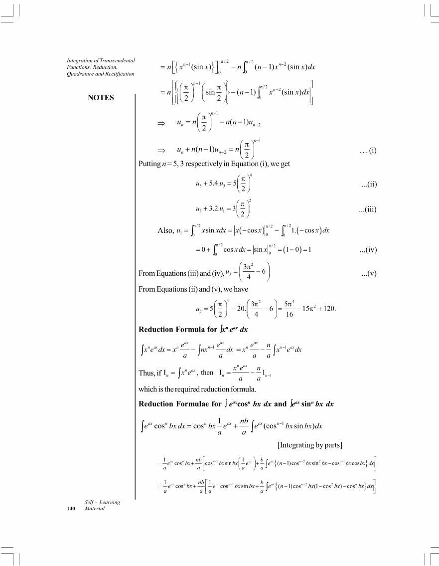
Integration of TranscendentalFunctions, Reduction,Quadrature and Rectification
NOTES
Self - Learning140 Material
/ 2 / 21 2
00(sin ) ( 1) (sin )n nn x x n n x x dx
1/ 2 2
0sin ( 1) (sin )
2 2
nnn n x x dx
1
2( 1)2
n
n nu n n n u
1
2( 1)2
n
n nu n n u n
… (i)
Putting n = 5, 3 respectively in Equation (i), we get4
5 35.4. 52
u u
...(ii)
2
3 13.2. 32
u u
...(iii)
Also, / 2
1 0sinu x xdx
/ 2/ 2
0 0cos 1. cosx x x dx
/ 2 / 2
000 cos sin 1 0 1x dx x
...(iv)
From Equations (iii) and (iv),2
3
36
4u
...(v)
From Equations (ii) and (v), we have4 2 4
25
3 55 20. 6 15 120.
2 4 16u
Reduction Formula for xn eax dx
1ax ax
n ax n ne ex e dx x nx dx
a a = 1
axn n axe n
x x e dxa a
Thus, if 1I , then I In ax
n axn n n
x e nx e
a a which is the required reduction formula.
Reduction Formulae for eaxcosn bx dx and eax sinn bx dx
11cos cos (cos sin )ax n n ax ax nnb
e bx dx bx e e bx bx dxa a
[Integrating by parts]
1 2 2 11 1cos cos sin ( 1)cos sin cos cosax n n ax ax n nnb b
e bx bx bx e e n bx bx bx bx dxa a a a
1 2 21 1cos cos sin ( 1)cos (1 cos ) cosax n ax n ax n nnb b
e bx e bx bx e n bx bx bx dxa a a a
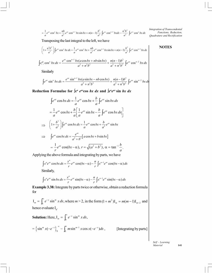
NOTES
Integration of TranscendentalFunctions, Reduction,
Quadrature and Rectification
Self - LearningMaterial 141
2 2 21 2
2 2 2
1cos cos sin ( 1) cos cosax n ax n ax n a x nnb b n b
e bx e bx bx n n e bxdx e bx dxa a a a
Transposing the last integral to the left, we have
2 2 21 2
2 2 2
11 cos cos cos sin ( 1) cosax n ax n ax n ax nn b nb b
e bx dx e bx e bx bx n n e bx dxa a a a
1 2
22 2 2 2 2 2
cos ( cos sin ) ( 1)cos cos
ax nax n ax ne bx a bx nb bx n n b
e bx dx e bx dxa n b a n b
Similarly
1 22
2 2 2 2 2 2
sin ( sin cos ) ( 1)sin sin
ax nax n ax ne bx a bx nb bx n n b
e bx dx e bx dxa n b a n b
Reduction Formulae for xn eaxcos bx dx and xneax sin bx dx
1cos cos sinax ax axb
e bx dx e bx e bx dxa a
1 1
cos sin cosax ax axb be bx e bx e bx dx
a a a a
2
2 2
11 cos cos sinax ax axb b
e bx dx e bx e bxa a a
2 2cos cos sin
axax e
e bx dx a bx b bxa b
= 2 2 11
cos( ), ( ), tanax be bx r a b
r a .
Applying the above formula and integrating by parts, we have
1cos cos( ) cos( )n
n ax ax n axx nx e bx dx e bx x e bx dx
r r
Similarly,
1sin sin( ) sin( )n
n ax ax n axx nx e bx dx e bx x e bx dx
r r
Example 3.38: Integrate by parts twice or otherwise, obtain a reduction formulafor
0I sin ,x m
m e x dx where m > 2, in the form 2
2(1 )I ( 1)Im mm m m and
hence evaluate I4.
Solution: Here,0
I sin ,x mm e x dx
= 1
0 0sin ( sin cos ( )m x m xx e m x x e dx
, [Integrating by parts]
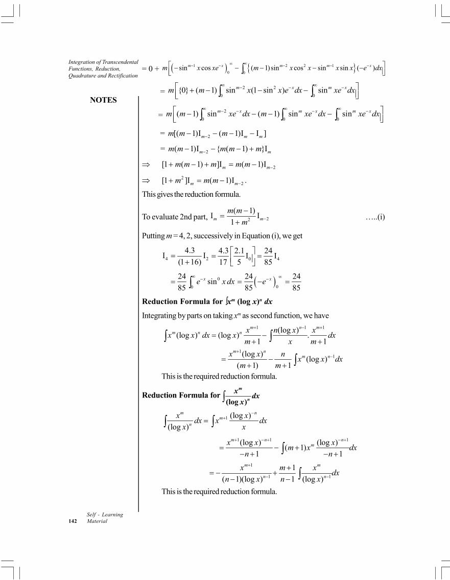
Integration of TranscendentalFunctions, Reduction,Quadrature and Rectification
NOTES
Self - Learning142 Material
= 0 + 1 2 2 1
0 0sin cos ( 1)sin cos sin sin ( )m x m m xm x xe m x x x x e dx
= 2 2
0 0{0} ( 1) sin (1 sin ) sinm x m xm m x x e dx xe dx
= 2
0 0 0( 1) sin ( 1) sin sinm x m x m xm m xe dx m xe dx xe dx
= 2[( 1)I ( 1)I I ]m m mm m m
= 2( 1)I { ( 1) }Im mm m m m m
2[1 ( 1) ]I ( 1)Im mm m m m m
22[1 ]I ( 1)Im mm m m .
This gives the reduction formula.
To evaluate 2nd part, 22
( 1)I I
1m m
m m
m
…..(i)
Putting m = 4, 2, successively in Equation (i), we get
4 2
4.3I I
(1 16)
0 4
4.3 2.1 24I I
17 5 85
0
0
24sin
85xe x dx
0
24 24
85 85xe
Reduction Formula for xm (log x)n dx
Integrating by parts on taking xm as second function, we have1 1 1(log )
(log ) (log ) .1 1
m n mm n n x n x x
x x dx x dxm x m
1
1(log )(log )
( 1) 1
m nm nx x n
x x dxm m
This is the required reduction formula.
Reduction Formula for(log )
m
n
xdx
x
1 (log )
(log )
m nm
n
x xdx x dx
x x
1 1 1(log ) (log )
( 1)1 1
m n nmx x x
m x dxn n
1
1 1
1
( 1)(log ) 1 (log )
m m
n n
x m xdx
n x n x
This is the required reduction formula.
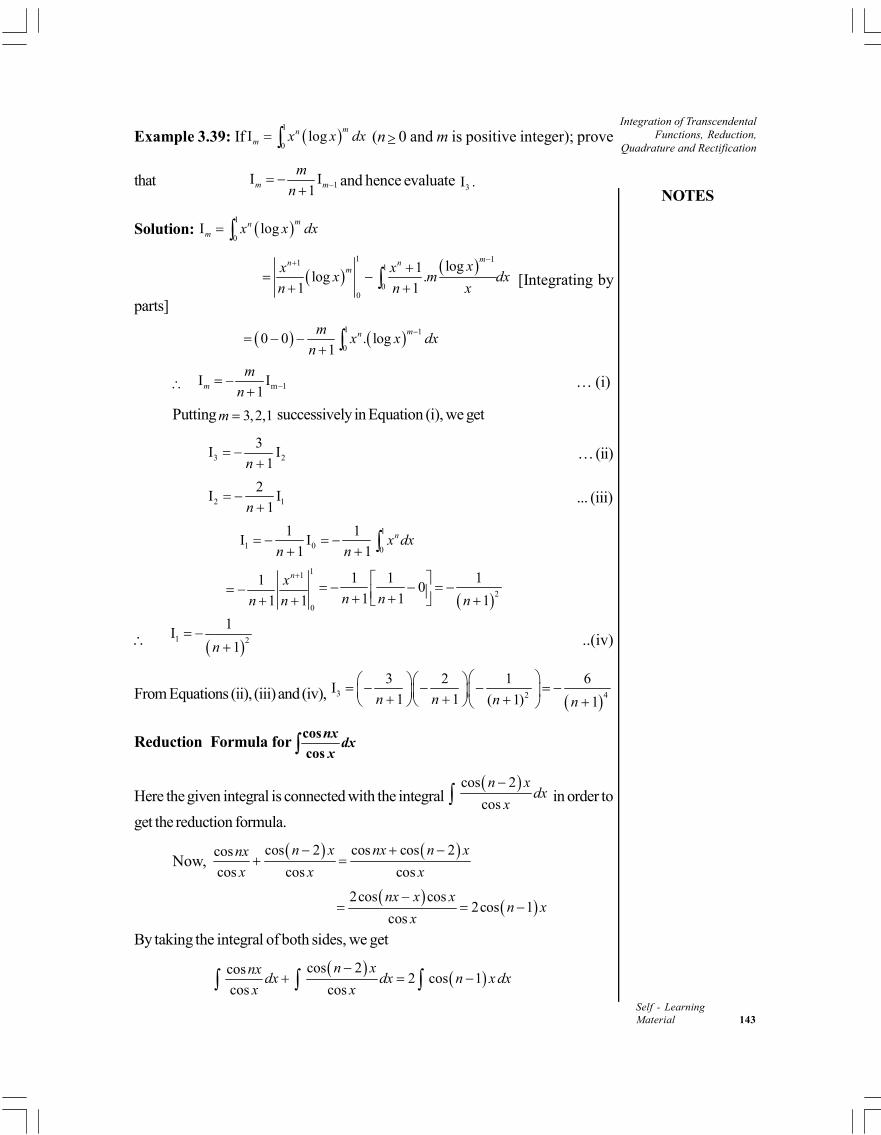
NOTES
Integration of TranscendentalFunctions, Reduction,
Quadrature and Rectification
Self - LearningMaterial 143
Example 3.39: If 1
0I log
mnm x x dx (n 0 and m is positive integer); prove
that 1I I1m m
m
n
and hence evaluate 3I .
Solution: 1
0I log
mnm x x dx
1 111
00
log1log .
1 1
mn nm xx x
x m dxn n x
[Integrating by
parts]
1 1
00 0 . log
1mnm
x x dxn
m 1I I1m
m
n
… (i)
Putting 3,2,1m successively in Equation (i), we get
3 2
3I I
1n
… (ii)
2 1
2I I
1n
... (iii)
1
1 0 0
1 1I I
1 1nx dx
n n
11
0
1
1 1
nx
n n
2
1 1 10
1 1 1n n n
1 2
1I
1n
..(iv)
From Equations (ii), (iii) and (iv), 3 2 4
3 2 1 6I
1 1 ( 1) 1n n n n
Reduction Formula forcos
cos
nxdx
x
Here the given integral is connected with the integral cos 2
cos
n xdx
x
in order to
get the reduction formula.
Now, cos 2 cos cos 2cos
cos cos cos
n x nx n xnx
x x x
2cos cos
2cos 1cos
nx x xn x
x
By taking the integral of both sides, we get
cos 2cos2 cos 1
cos cos
n xnxdx dx n x dx
x x
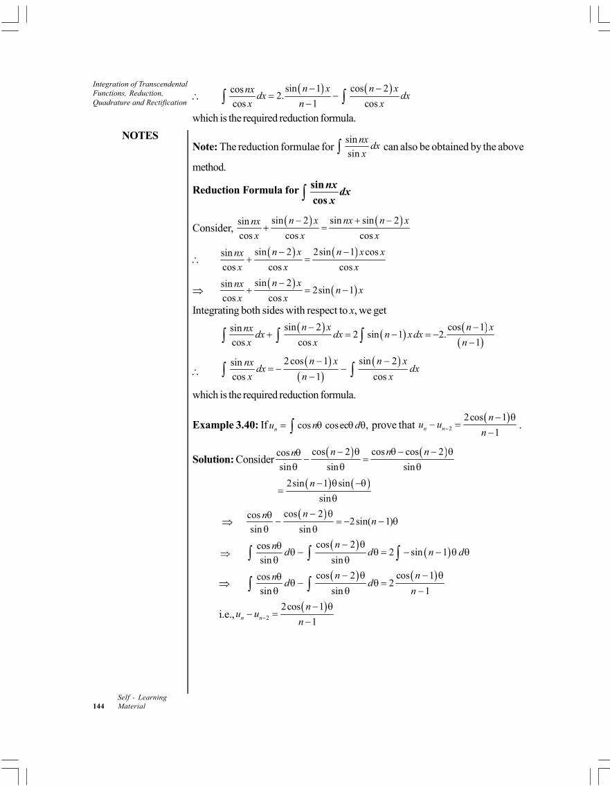
Integration of TranscendentalFunctions, Reduction,Quadrature and Rectification
NOTES
Self - Learning144 Material
sin 1 cos 2cos
2.cos 1 cos
n x n xnxdx dx
x n x
which is the required reduction formula.
Note: The reduction formulae forsin
sin
nxdx
x can also be obtained by the above
method.
Reduction Formula for nxdx
x
sin
cos
Consider, sin 2 sin sin 2sin
cos cos cos
n x nx n xnx
x x x
sin 2 2sin 1 cossin
cos cos cos
n x n x xnx
x x x
sin 2sin
2sin 1cos cos
n xnxn x
x x
Integrating both sides with respect to x, we get
sin 2 cos 1sin2 sin 1 2.
cos cos 1
n x n xnxdx dx n xdx
x x n
2cos 1 sin 2sin
cos 1 cos
n x n xnxdx dx
x n x
which is the required reduction formula.
Example 3.40: If cos cosec ,nu n d prove that
2
2cos 1
1n n
nu u
n
.
Solution: Consider cos 2 cos cos 2cos
sin sin sin
n n nn
2sin 1 sin
sin
n
cos 2cos
2sin( 1)sin sin
nnn
cos 2cos2 sin 1
sin sin
nnd d n d
cos 2 cos 1cos
2sin sin 1
n nnd d
n
i.e.,
2
2cos 1
1n n
nu u
n
NOTES
Integration of TranscendentalFunctions, Reduction,
Quadrature and Rectification
Self - LearningMaterial 145
Reduction Formula for ( )m n px a bx dx pm nx a bx dx can be connected with any one of the following six integrals:
(i) 1pm nx a bx dx
(ii) 1pm nx a bx dx
(iii) pm n nx a bx dx (iv) 1pm n nx a bx dx
(v) pm n nx a bx dx (vi) 1pm n nx a bx dx
We cannot connect the given integral to that in which the indices of
both na bx and mx are increased or decreased.
Method to connect p
m nx a bx dx with any integral of the above type
Step 1: Let 11P nx a bx , where is smaller of the two indices of x and
is smaller of the two indices of na bx .
Step 2: After defining P, differentiate P with respect to x to get Pd
dx. Express it in
terms of integrands of the two integrals to be connected.
Step 3: Integrate both sides with respect to x and solve to get the value of thegiven integral.
Example 3.41: Prove that
1 122 2 2 2 2 2 2
2 3
2 12 1n n n
ndx x dx
a na x a n a x a x
Solution: Let us connect 2 2 n
dx
a x with 12 2 n
dx
a x
Now
0 2 2
2 2
n
n
dxx a x dx
a x
and
10 2 2
12 2
n
n
dxx a x dx
a x
i.e.,
12 2
12 2P
n
n
xx a x
a x
...(i)
12 2 2 2P1 .2
n nda x x n a x x
dx
2
12 2 2 2
12 1
n n
xn
a x a x
Integration of TranscendentalFunctions, Reduction,Quadrature and Rectification
NOTES
Self - Learning146 Material
2 2 2
12 2 2 2
12 1
n n
a x an
a x a x
2
1 12 2 2 2 2 2
2 1 2 11n n n
n a n
a x a x a x
2
12 2 2 2
2 1P 3 2n n
a nd n
dx a x a x
Integrating both sides, we get
2
12 2 2 2
1 1P 3 2 2 1
n nn dx a n dx
a x a x
2
12 2 2 2
1 12 1 P (3 2 )
n na n dx n dx
a x a x
… (ii)
Using Equations (i) in (ii) and dividing by 22 1a n , we get
1 122 2 2 2 2 2 2
2 31 1
2 12 1n n n
nxdx dx
a na x a n a x a x
=
1 2 12 2 2 2 2
2 3 1
2 12 1n n
nxdx
a na n a x a x
Check Your Progress
9. If logn
nu x dx , find the value of 1n nu n u .
10. Connect pm nx a bx dx with 1pm nx a bx dx
11. If 1/ 2I ( ) ,nn x a x dx prove that
3 / 21(2 3)I 2 I 2 ( )n
n nn an x a x
12. If 0
I sin(2 1)nn x p xdx
, prove that
1
22 2
( 1)I I ( 1)
2(2 1) (2 1)
np
n n
n n n
p p
, n and p being positive
integers.
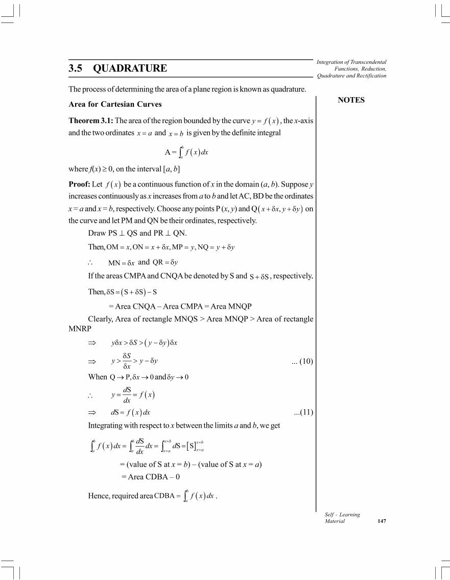
NOTES
Integration of TranscendentalFunctions, Reduction,
Quadrature and Rectification
Self - LearningMaterial 147
3.5 QUADRATURE
The process of determining the area of a plane region is known as quadrature.
Area for Cartesian Curves
Theorem 3.1: The area of the region bounded by the curve y f x , the x-axis
and the two ordinates x a and x b is given by the definite integral
A = b
af x dx
where f(x) 0, on the interval [a, b]
Proof: Let f x be a continuous function of x in the domain (a, b). Suppose y
increases continuously as x increases from a to b and let AC, BD be the ordinates
x = a and x = b, respectively. Choose any points P (x, y) and Q ,x x y y on
the curve and let PM and QN be their ordinates, respectively.
Draw PS QS and PR QN.
Then,OM , ON , MP , NQx x x y y y
MN x and QR y
If the areas CMPA and CNQA be denoted by S and S S , respectively..
Then, S S S S
= Area CNQA – Area CMPA = Area MNQP
Clearly, Area of rectangle MNQS > Area MNQP > Area of rectangleMNRP
y x S y y x
S
y y yx
... (10)
When Q P, 0x and 0y
Sdy f x
dx
Sd f x dx ...(11)
Integrating with respect to x between the limits a and b, we get
SS S
b b x b x b
x aa a x a
df x dx dx d
dx
= (value of S at x = b) – (value of S at x = a)
= Area CDBA – 0
Hence, required area CDBAb
af x dx .
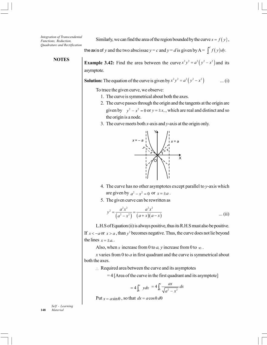
Integration of TranscendentalFunctions, Reduction,Quadrature and Rectification
NOTES
Self - Learning148 Material
Similarly, we can find the area of the region bounded by the curve x f y ,
the axis of y and the two abscissae y = c and y = d is given by A = .d
cf y dy
Example 3.42: Find the area between the curve 2 2 2 2 2x y a y x and its
asymptote.
Solution: The equation of the curve is given by 2 2 2 2 2x y a y x ... (i)
To trace the given curve, we observe:1. The curve is symmetrical about both the axes.2. The curve passes through the origin and the tangents at the origin are
given by 2 2 0y x or ,y x , which are real and distinct and so
the origin is a node.3. The curve meets both x-axis and y-axis at the origin only.
Y
x a = x – a =
y x =
XO
y– x
=
4. The curve has no other asymptotes except parallel to y-axis whichare given by 2 2 0a x or x a .
5. The given curve can be rewritten as
2 2 2 2
2
2 2
a x a xy
a x a xa x
... (ii)
L.H.S of Equation (ii) is always positive, thus its R.H.S must also be positive.
If x a or x a , than 2y becomes negative. Thus, the curve does not lie beyond
the lines .x a .
Also, when x increase from 0 to a, y increase from 0 to .
x varies from 0 to a in first quadrant and the curve is symmetrical aboutboth the axes.
Required area between the curve and its asymptotes
= 4 [Area of the curve in the first quadrant and its asymptote]
04
aydx 0 2 2
4a ax
dxa x
Put sinx a , so that cosdx a d

NOTES
Integration of TranscendentalFunctions, Reduction,
Quadrature and Rectification
Self - LearningMaterial 149
Now for x = 0, 0 and for ,2
x a
Required area = / 2
0
. sin4 . cos
cos
a aa d
a
= / 2/ 22 2
004 sin 4 cosa d a
= 2 24 0 1 4a a
Area between Two Curves
Let f and g be the two functions (Refer Figure 3.1) which are continuous on the
interval [a,b]. If f and g both are positive and f x g x for all values of x in
interval [a, b]. Then, the area between two graphs is given by
A = b b
a af x dx g x dx
b
af x g x dx
Y
d
c
O
g f
X
Fig. 3.1 Area of Boundary Curves
I II
b
ay y dx
Note: If the boundary curves are functions of y, then the required area is given by
the integral d
cf y g y dy .
Corollary: Now, we derive a formula for the regions where neither f nor g remainspositive and also neither function remains greater than the other (Refer Figure3.2).
Y
O
f
a g
g
f
f
gb X
Fig. 3.2 Derivation of Formula for Regions
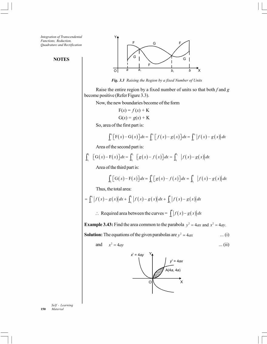
Integration of TranscendentalFunctions, Reduction,Quadrature and Rectification
NOTES
Self - Learning150 Material
Y
O
F
a
G
G
F
F
G
Xb1 ba1
Fig. 3.3 Raising the Region by a fixed Number of Units
Raise the entire region by a fixed number of units so that both f and gbecome positive (Refer Figure 3.3).
Now, the new boundaries become of the form
F(x) = f (x) + K
G(x) = g(x) + K
So, area of the first part is:
1 1 1
F Ga a a
a a ax x dx f x g x dx f x g x dx
Area of the second part is:
1 1
1 1
G Fb b
a ax x dx g x f x dx 1
1
b
af x g x dx
Area of the third part is:
1 1
G Fb b
b bx x dx g x f x dx
1
b
bf x g x dx
Thus, the total area:
1 1
1 1
a b b
a a bf x g x dx f x g x dx f x g x dx
Required area between the curves = b
af x g x dx
Example 3.43: Find the area common to the parabola 2 24 and 4 .y ax x ay
Solution: The equations of the given parabolas are 2 4y ax ... (i)
and 2 4x ay ... (ii)
x ay2 = 4 Y
y ax2 = 4
A(4 , 4 )a a
XO
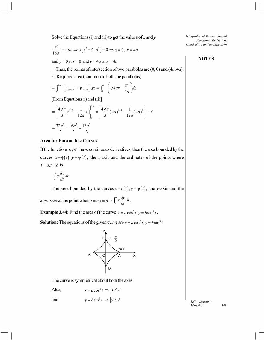
NOTES
Integration of TranscendentalFunctions, Reduction,
Quadrature and Rectification
Self - LearningMaterial 151
Solve the Equations (i) and (ii) to get the values of x and y
4
24
16
xax
a 3 364 0x x a 0, 4x x a
and 0at 0 and 4 at 4y x y a x a
Thus, the points of intersection of two parabolas are (0, 0) and (4a, 4a).
Required area (common to both the parabolas)
4
0
a
upper lowery y dx 2
4
04
4
a xax dx
a
[From Equations (i) and (ii)]4
3/ 2 3
0
4 1
3 12
a
ax x
a
3/ 2 34 14 4 0
3 12
aa a
a
2 2 232 16 16
3 3 3
a a a
Area for Parametric Curves
If the functions , have continuous derivatives, then the area bounded by the
curves , ,x t y t the x-axis and the ordinates of the points where
,t a t b is
b
a
dxy dt
dt
The area bounded by the curves , ,x t y t the y-axis and the
abscissae at the point when ,t c t d isd
c
dyx dt
dt .
Example 3.44: Find the area of the curve 3 3cos , sinx a t y b t .
Solution: The equations of the given curve are 3 3cos , sinx a t y b t
Y
B
O A X
t = 0
t =
The curve is symmetrical about both the axes.
Also, 3cosx a t x a
and 3siny b t y b
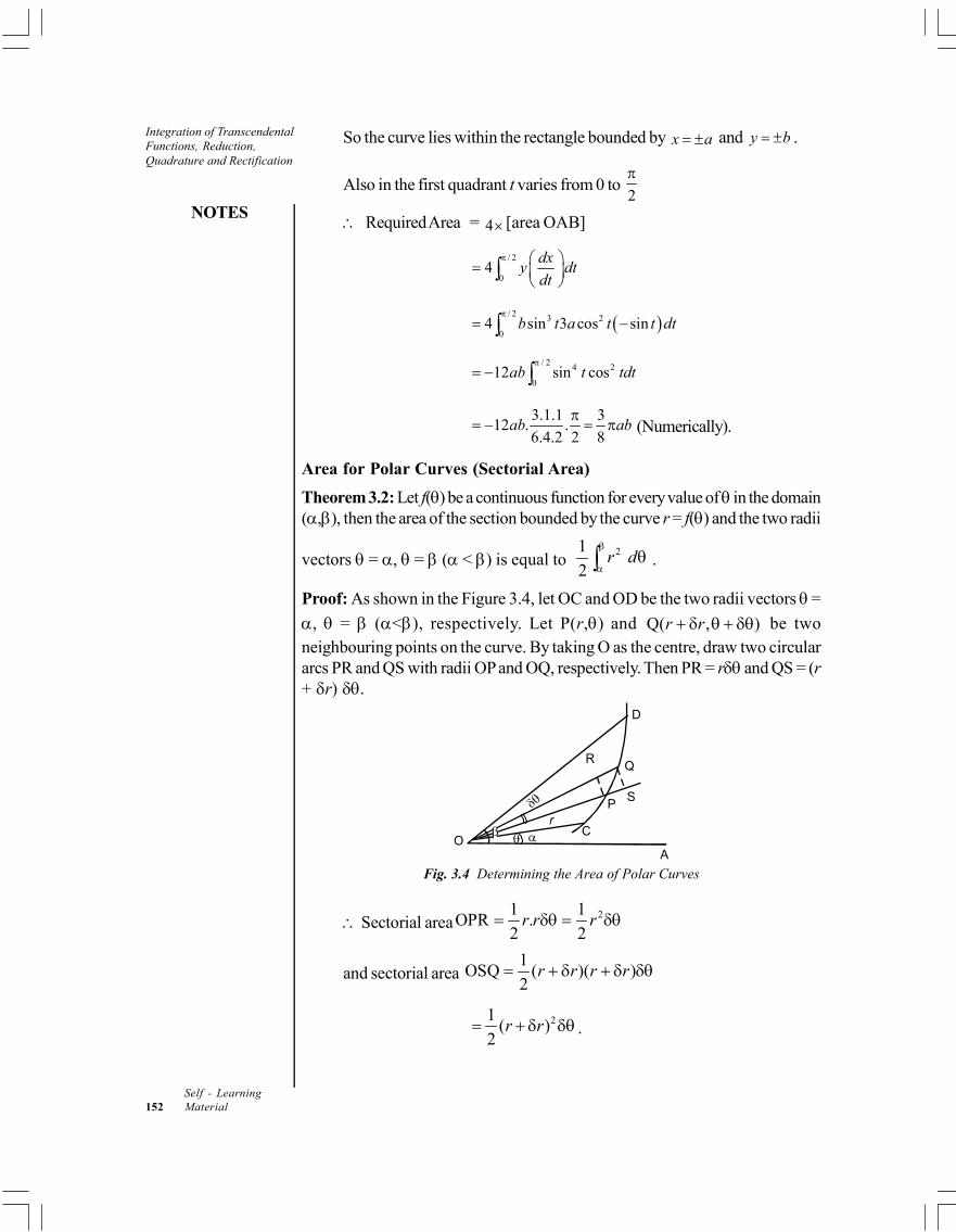
Integration of TranscendentalFunctions, Reduction,Quadrature and Rectification
NOTES
Self - Learning152 Material
So the curve lies within the rectangle bounded by x a and y b .
Also in the first quadrant t varies from 0 to 2
Required Area = 4 [area OAB]
/ 2
04
dxy dt
dt
/ 2 3 2
04 sin 3 cos sinb t a t t dt
/ 2 4 2
012 sin cosab t tdt
3.1.1 312 . .
6.4.2 2 8ab ab
(Numerically).
Area for Polar Curves (Sectorial Area)
Theorem 3.2: Let f() be a continuous function for every value of in the domain(,), then the area of the section bounded by the curve r = f() and the two radii
vectors = , = ( < ) is equal to 21
2r d
.
Proof: As shown in the Figure 3.4, let OC and OD be the two radii vectors =
, = (<), respectively. Let P(r,) and Q( , )r r be twoneighbouring points on the curve. By taking O as the centre, draw two circulararcs PR and QS with radii OP and OQ, respectively. Then PR = r and QS = (r+ r) .
D
RQ
PS
C
A
r
O
Fig. 3.4 Determining the Area of Polar Curves
Sectorial area21 1
OPR .2 2
r r r
and sectorial area 1
OSQ ( )( )2
r r r r
21
( )2
r r .
NOTES
Integration of TranscendentalFunctions, Reduction,
Quadrature and Rectification
Self - LearningMaterial 153
Let A and A + A denote the area of sectors OCP and OCQ respectively,then A = Area OCQ Area OCP
= Area OPQ
Also, the area OPQ lies between the areas OSQ and OPR
2 21 1( )
2 2r r A r
2 2( )
2 2
r r A r
… (12)
Since, f() is a continuous function so, as 0 and r 0
2A
2
d r
d
21
2r d dA .
On integrating both sides between the limits = , = , we get
21 A
[A]2
dr d d
d
= (Value of A when = ) (Value of A when = )
= Area of OCD
Hence, sectorial area OCD = 21
2r d
.
Note: The following points should be remembered while doing the problems forpolar curves:
1. It is easy to transform a cartesian equation to polar form than to solvefor y in some cases.
2. To obtain the limits of integration for a loop, find two successive valuesof for which r = 0.
3. If the curve is symmetrical about the x-axis only, evaluate the integralfrom 0 to and multiply the result by 2.
4. If the curve is symmetrical about both the axes, evaluate the integral
from 0 to2
and multiply the result by 4.
5. If n is odd, the curve cosr a n or sinr a n have n equal loopsand if n is even the curve have 2n equal loops.
Example 3.45: Find the area of one loop of the curve r = a sin 3.
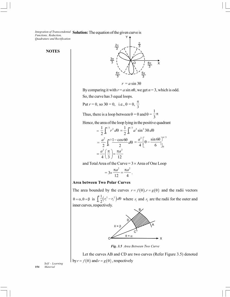
Integration of TranscendentalFunctions, Reduction,Quadrature and Rectification
NOTES
Self - Learning154 Material
Solution: The equation of the given curve isY
XO
r = a sin 3
By comparing it with r = a sin n, we get n = 3, which is odd.
So, the curve has 3 equal loops.
Put r = 0, so 3 = 0, i.e., = 0, 3
Thus, there is a loop between = 0 and = 1
3
Hence, the area of the loop lying in the positive quadrant
= / 3 2
0
1
2r d
/ 3 2 2
0
1sin
2a d
= 2
0
1 cos 6
2 2
ad
/ 32
0
sin 6
4 6
a
2 2
4 3 12
a a
and Total Area of the Curve = 3 Area of One Loop
= 32 2
12 4
a a .
Area between Two Polar Curves
The area bounded by the curves ,r f r g and the radii vectors
, is 2 21 2
1
2r r d
where 1r and 2r are the radii for the outer and
inner curves, respectively.B
D
A
C
XO
Fig. 3.5 Area Between Two Curve
Let the curves AB and CD are two curves (Refer Figure 3.5) denoted
by r f and r g , respectively
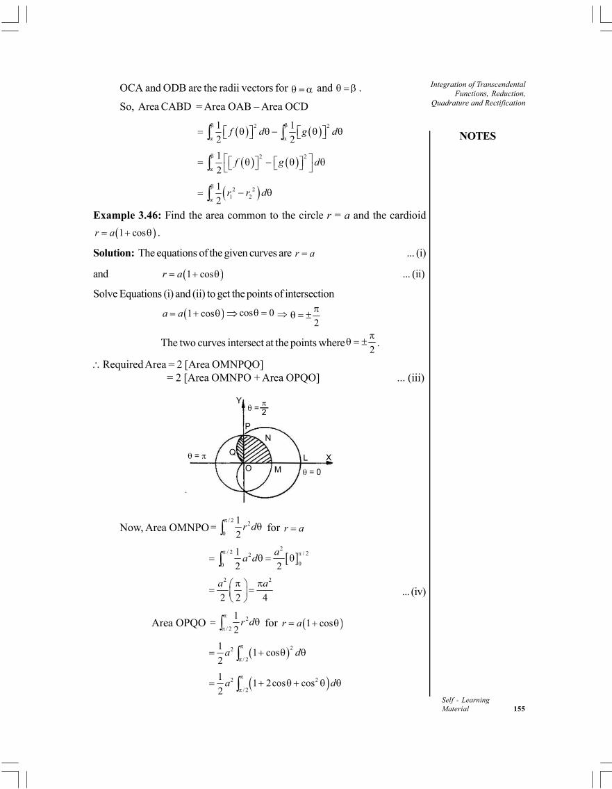
NOTES
Integration of TranscendentalFunctions, Reduction,
Quadrature and Rectification
Self - LearningMaterial 155
OCA and ODB are the radii vectors for and .
So, Area CABD = Area OAB – Area OCD
2 21 1
2 2f d g d
2 21
2f g d
2 21 2
1
2r r d
Example 3.46: Find the area common to the circle r = a and the cardioid
1 cosr a .
Solution: The equations of the given curves are r a ... (i)
and 1 cosr a ... (ii)
Solve Equations (i) and (ii) to get the points of intersection
1 cosa a cos 0 2
The two curves intersect at the points where2
.
Required Area = 2 [Area OMNPQO] = 2 [Area OMNPO + Area OPQO] ... (iii)
Y
PN
Q
O ML X
Now, Area OMNPO/ 2 2
0
1
2r d
for r a
2
/ 2 / 22
00
1
2 2
aa d
2 2
2 2 4
a a
... (iv)
Area OPQO 2
/ 2
1
2r d
for 1 cosr a
22
/ 2
11 cos
2a d
2 2
/ 2
11 2cos cos
2a d
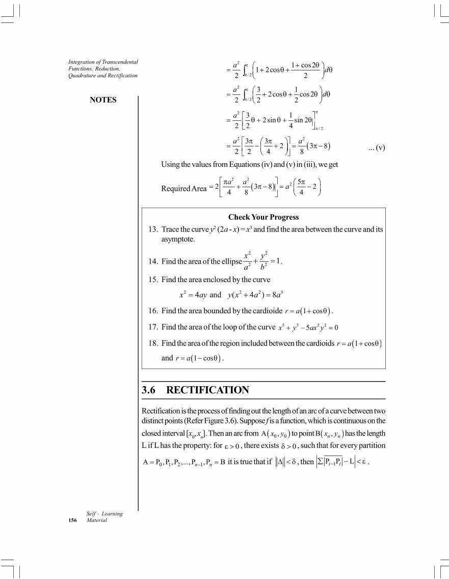
Integration of TranscendentalFunctions, Reduction,Quadrature and Rectification
NOTES
Self - Learning156 Material
2
/ 2
1 cos21 2cos
2 2
ad
2
/ 2
3 12cos cos2
2 2 2
ad
2
/ 2
3 12sin sin 2
2 2 4
a
2 23 3
2 3 82 2 4 8
a a ... (v)
Using the values from Equations (iv) and (v) in (iii), we get
Required Area 2 2
2 52 3 8 2
4 8 4
a aa
Check Your Progress
13. Trace the curve y2 (2a - x) = x3 and find the area between the curve and itsasymptote.
14. Find the area of the ellipse2 2
2 21
x y
a b .
15. Find the area enclosed by the curve
2 2 2 34 and ( 4 ) 8x ay y x a a
16. Find the area bounded by the cardioide 1 cosr a .
17. Find the area of the loop of the curve 5 5 2 25 0x y ax y
18. Find the area of the region included between the cardioids 1 cosr a
and 1 cosr a .
3.6 RECTIFICATION
Rectification is the process of finding out the length of an arc of a curve between twodistinct points (Refer Figure 3.6). Suppose f is a function, which is continuous on the
closed interval [x0, x
n]. Then an arc from 0 0A ,x y to point B ,n nx y has the length
L if L has the property: for 0 , there exists 0 , such that for every partition
0 1 2 1A P ,P ,P ,...,P ,P Bn n it is true that if , then 1P P Li i .
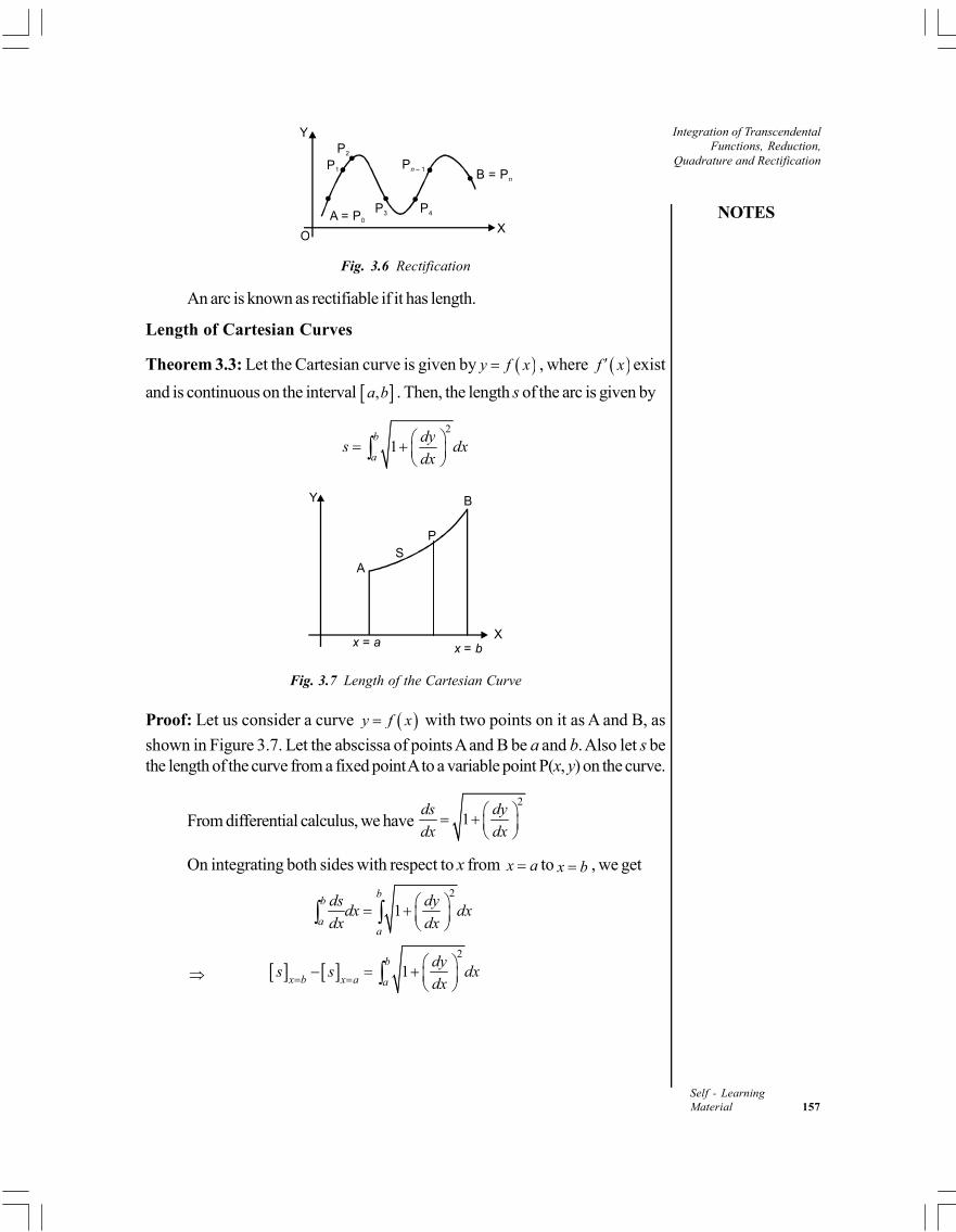
NOTES
Integration of TranscendentalFunctions, Reduction,
Quadrature and Rectification
Self - LearningMaterial 157
YP2
P1 Pn – 1B = Pn
A = P0
P3 P4
XO
Fig. 3.6 Rectification
An arc is known as rectifiable if it has length.
Length of Cartesian Curves
Theorem 3.3: Let the Cartesian curve is given by y f x , where f x exist
and is continuous on the interval ,a b . Then, the length s of the arc is given by
2
1b
a
dys dx
dx
Y B
PS
A
x a = x b = X
Fig. 3.7 Length of the Cartesian Curve
Proof: Let us consider a curve y f x with two points on it as A and B, as
shown in Figure 3.7. Let the abscissa of points A and B be a and b. Also let s bethe length of the curve from a fixed point A to a variable point P(x, y) on the curve.
From differential calculus, we have 2
1ds dy
dx dx
On integrating both sides with respect to x from x a to x b , we get
2
1b
b
aa
ds dydx dx
dx dx
2
1b
x b x a a
dys s dx
dx
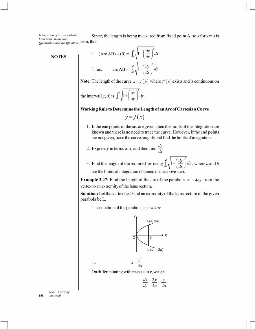
Integration of TranscendentalFunctions, Reduction,Quadrature and Rectification
NOTES
Self - Learning158 Material
Since, the length is being measured from fixed point A, so s for x = a iszero, thus
(Arc AB) – (0) = 2
1b
a
dydx
dx
Thus, arc AB = 2
1b
a
dydx
dx
Note: The length of the curve x f y where f y exists and is continuous on
the interval [c, d] is 2
1d
c
dxdy
dy
.
Working Rule to Determine the Length of an Arc of Cartesian Curve
y f x
1. If the end points of the arc are given, then the limits of the integration areknown and there is no need to trace the curve. However, if the end pointsare not given, trace the curve roughly and find the limits of integration.
2. Express y in terms of x, and then find dy
dx.
3. Find the length of the required arc using2
1b
a
dydx
dx , where a and b
are the limits of integration obtained in the above step.
Example 3.47: Find the length of the arc of the parabola 2 4y ax from the
vertex to an extremity of the latus rectum.
Solution: Let the vertex be O and an extremity of the latus rectum of the givenparabola be L.
The equation of the parabola is 2 4y ax
YL(a, 2a)
XSO
2
4
yx
a
On differentiating with respect to y, we get
2
4 2
dx y y
dy a a
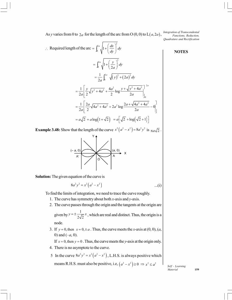
NOTES
Integration of TranscendentalFunctions, Reduction,
Quadrature and Rectification
Self - LearningMaterial 159
As y varies from 0 to 2a for the length of the arc from O (0, 0) to L ,2a a ,
Required length of the arc 2
2
01
a dxdy
dy
2
2
01
2
a ydy
a
2 2 2
0
12
2
ay a dy
a
22 22
2 2
0
41 44 log
2 2 2 2
a
y y ay ay a
a a
2 22 2 21 2 2 4 4
4 4 2 log 02 2 2
a a a aa a a
a a
2 log 1 2a a 2 log 2 1a
Example 3.48: Show that the length of the curve 2 2 2 2 28x a x a y is 2a .
Y
( , 0)aX
AO
(– , 0)a
Solution: The given equation of the curve is
2 2 2 2 28a y x a x ...(i)
To find the limits of integration, we need to trace the curve roughly.1. The curve has symmetry about both x-axis and y-axis.2. The curve passes through the origin and the tangents at the origin are
given by1
2 2y x , which are real and distinct. Thus, the origin is a
node.
3. If 0, then 0,y x a . Thus, the curve meets the x-axis at (0, 0), (a,0) and (–a, 0).
If 0, then 0x y . Thus, the curve meets the y-axis at the origin only..
4. There is no asymptote to the curve.
5 In the curve 2 2 2 2 28a y x a x , L.H.S. is always positive which
means R.H.S. must also be positive, i.e, 2 2 0a x 2 2x a
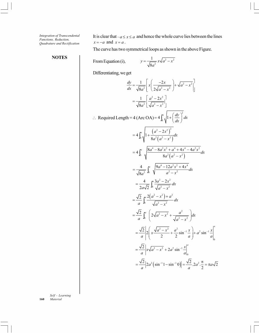
Integration of TranscendentalFunctions, Reduction,Quadrature and Rectification
NOTES
Self - Learning160 Material
It is clear that –a x a and hence the whole curve lies between the linesx a and x a .
The curve has two symmetrical loops as shown in the above Figure.
From Equation (i), 2 2
2
1
8y x a x
a
Differentiating, we get
2 2
2 2 2
1 2
8 2
dy xx a x
dx a a x
2 2
2 2 2
1 2
8
a x
a a x
Required Length = 4 (Arc OA)2
04 1
a dydx
dx
22 2
2 2 20
24 1
8
a a xdx
a a x
4 2 2 4 4 2 2
2 2 20
8 8 4 44
8
a a a x a x a xdx
a a x
4 2 2 4
2 22 0
4 9 12 4
8
a a a x xdx
a xa
2 2
0 2 2
4 3 2
2 2
a a xdx
a a x
2 2 2
0 2 2
22 a a x adx
a a x
2
2 2
0 2 2
22
a aa x dx
a a x
2 2 2
1 2 1
0
22 sin sin
2 2
a
a x a x xx a
a a a
2 2 2 1
0
22 sin
ax
x a x aa a
2 1 1 22 22 sin 1 sin 0 .2 . 2
2a a a
a a
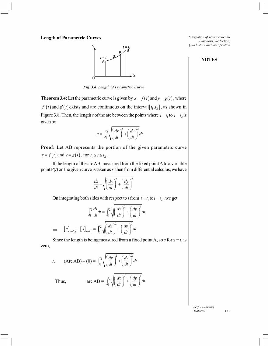
NOTES
Integration of TranscendentalFunctions, Reduction,
Quadrature and Rectification
Self - LearningMaterial 161
Length of Parametric Curves
Y
O
t t = 1
A
SP
t t = 2
B
X
Fig. 3.8 Length of Parametric Curve
Theorem 3.4: Let the parametric curve is given by x f t and y g t , where
f t and g t exists and are continuous on the interval 1 2,t t , as shown in
Figure 3.8. Then, the length s of the arc between the points where 1t t to 2t t isgiven by
2 22
1
t
t
dx dys dt
dt dt
Proof: Let AB represents the portion of the given parametric curve
x f t and y g t , for 1 2t t t .
If the length of the arc AB, measured from the fixed point A to a variablepoint P(t) on the given curve is taken as s, then from differential calculus, we have
2 2ds dx dy
dt dt dt
On integrating both sides with respect to t from 1t t to 2t t , we get
2 22 2
1 1
t t
t t
ds dx dydt dt
dt dt dt
2 2
2
2 1 1
t
x t x t t
dx dys s dt
dt dt
Since the length is being measured from a fixed point A, so s for x = t1 is
zero,
(Arc AB) – (0) = 2 2
2
1
t
t
dx dydt
dt dt
Thus, arc AB = 2 2
2
1
t
t
dx dydt
dt dt
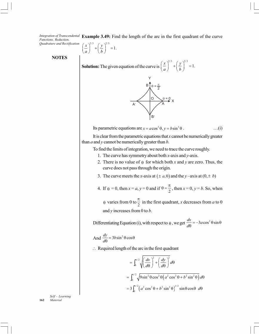
Integration of TranscendentalFunctions, Reduction,Quadrature and Rectification
NOTES
Self - Learning162 Material
Example 3.49: Find the length of the arc in the first quadrant of the curve2 / 3 2 / 3
1.x y
a b
Solution: The given equation of the curve is 2 / 3 2 / 3
1.x y
a b
Y
B
AX
O
Its parametric equations are 3 3cos , sinx a y b . …(i)
It is clear from the parametric equations that x cannot be numerically greaterthan a and y cannot be numerically greater than b.
To find the limits of integration, we need to trace the curve roughly.1. The curve has symmetry about both x-axis and y-axis.2. There is no value of for which both x and y are zero. Thus, the
curve does not pass through the origin.
3. The curve meets the x-axis at ,0a and the y –axis at (0, b)
4. If = 0, then x = a, y = 0 and if 2
, then x = 0, y = b. So, when
varies from 0 to2
in the first quadrant, x decreases from a to 0
and y increases from 0 to b.
Differentiating Equation (i), with respect to , we get 23 cos sindx
ad
And 23 sin cosdy
bd
Required length of the arc in the first quadrant
2 2
/ 2
0
dx dyd
d d
/ 2 2 2 2 2 2 2
09sin cos cos sina b d
/ 2 1/ 22 2 2 2
03 cos sin sin cosa b d
NOTES
Integration of TranscendentalFunctions, Reduction,
Quadrature and Rectification
Self - LearningMaterial 163
2 2 2 2 2
2 2Put cos sin andsin cos
zdza b z d
b a
.
Also, when 0, and when ,2
z a z b
Length of the arc in the first quadrant 2 23 .
b
a
zdzz
b a
2
2 2
3 b
az dz
b a
3
2 2
3
3
b
a
z
b a
3 3
2 2
b a
b a
2 2 2 2b a b ba a a ab b
b a b a a b
Length of Polar Curves
Theorem 3.5: Let the polar curve is given by r f , where f and f are
continuous on a interval , . Then the length s of arc of the curve between the
points for which to is given by 2
2 drs r d
d
Proof: The given equation of the curve is r f .
We know that cosx r , siny r …(13)
Differentiating with respect to , we get
sin cosdx dr
rd d
…(14)
and cos sindy dr
rd d
…(15)
Also, we know that the length s of the parametric curve from to isgiven by
2 2
dx dys d
d d
On substituting the values from Equations (14) and (15), we get
s 2 2
sin cos cos sindr dr
r r dd d
On solving, we get 2
2 drs r d
d
which is the required equation for finding out the length of an arc of the polarcurve.
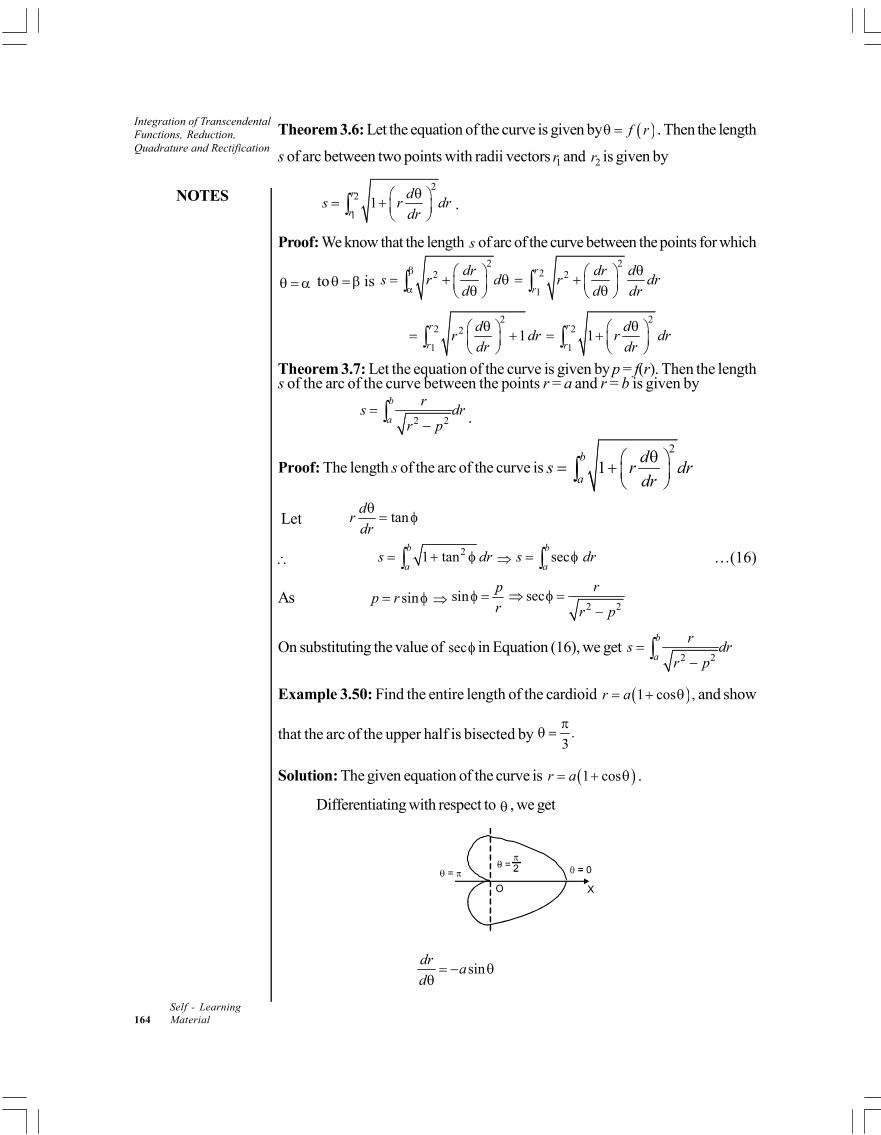
Integration of TranscendentalFunctions, Reduction,Quadrature and Rectification
NOTES
Self - Learning164 Material
Theorem 3.6: Let the equation of the curve is given by f r . Then the length
s of arc between two points with radii vectors 1r and 2r is given by
2
2
11
r
r
ds r dr
dr
.
Proof: We know that the length s of arc of the curve between the points for which
to is 2
2 drs r d
d
2
2 2
1
r
r
dr dr dr
d dr
2
2 2
11
r
r
dr dr
dr
22
11
r
r
dr dr
dr
Theorem 3.7: Let the equation of the curve is given by p = f(r). Then the lengths of the arc of the curve between the points r = a and r = b is given by
2 2
b
a
rs dr
r p
.
Proof: The length s of the arc of the curve is2
1b
a
ds r dr
dr
Let tand
rdr
21 tanb
as dr sec
b
as dr …(16)
As sinp r sinp
r
2 2sec
r
r p
On substituting the value of sec in Equation (16), we get 2 2
b
a
rs dr
r p
Example 3.50: Find the entire length of the cardioid 1 cos ,r a and show
that the arc of the upper half is bisected by .3
Solution: The given equation of the curve is 1 cosr a .
Differentiating with respect to , we get
XO
sindr
ad
NOTES
Integration of TranscendentalFunctions, Reduction,
Quadrature and Rectification
Self - LearningMaterial 165
Length of whole arc = 2Length of upper half2
2
02
drr d
d
22 2 2
02 1 cos sina a d
0
2 2 1 cosa d
00
4 cos 4 2sin2 2
a d a
8 1 0 8a a
Since the complete length of cardioid is 8a, thus the length of the upper halfis 4a.
The length s of arc from 0 to3
is
2/ 3 2
0
drs r d
d
/3
02 cos
2a d
/3
0
2 2sin2
a
14 0 2
2a a
1
2 ×Length of the upper half arc
Thus, the length of the upper half arc is bisected at .3
Check Your Progress
19. Find the length of the arc 2 2 2 0x y ax in the first quadrant.
20. Find the length of the loop of the curve 223 .ay x x a
21. Find the length of the arc of the curve x = e sin , y = e sin from
0 to .2
22. Find the whole length of the asteroid 2 / 3 2 / 3 2 / 3.x y a 23. Find the whole length of the curve 1 cosr a and show that the arc of
the upper half of the curve is bisected by 2
3
.
24. Find the length of arc of the equiangular spiral cotr ae between the points
for which the radii vectors are 1r and 2 .r
Integration of TranscendentalFunctions, Reduction,Quadrature and Rectification
NOTES
Self - Learning166 Material
3.7 ANSWERS TO ‘CHECK YOUR PROGRESS’
1. To give a precise shape to the definition of integration, we observe. If g (x)is a function of x such that,
d
dx g (x) = f (x)
then we define integral of f (x) with respect to x, to be the function g (x).This is put in the notational form as,
( )f x dx = g (x)
The function f (x) is called the Integrand. Presence of dx is there just toremind us that integration is being done with respect to x.
2. (a) (i) 2 x (ii) 2
x
(iii)3 / 2 5 / 22 2
3 5
x x(iv)
4 2
8 4
ax bx
(b) (i)2
2
xe(ii)
2 3
2
xe(iii) xe
(c) (i) 1 21 (sin )2
x (ii) sin (log x) (iii) tan–1 ex
3. (a) (i) sin h–1 (x + 1) (ii) 13 sin h–1
3 2
5
x
(iii) 12 sin2
x
a
(b) (i)1
8(4x – 3) 22 3 4x x +
412
32sin–1
4 3
41
x
(ii) 2
x 2 3
2 33
x sin–1 3
2
x
(iii) 2 19 29 4 sin
2 4 3
x xx
4. (i) 1
6(ii)
64
35(iii)
2
3
5.22
cosec cot cot3
NOTES
Integration of TranscendentalFunctions, Reduction,
Quadrature and Rectification
Self - LearningMaterial 167
6.2tan
log sec2
xx
7. 1
3n
8.5
32
9. logn
x x
10.
11
1 1
pm npm n
x a bx pnax a bx dx
m pn m pn
11. Here, connect 3/ 2( )nx a x dx with 1 1/ 2( )nx a x dx .
Let 1 1 1/ 2 1 3 / 2P ( ) ( )n nx a x x a x
1 3 / 2 1/ 2P 3( ) ( )
2n nd
nx a x x a xdx
1 1/ 2 1/ 23( ) ( ) ( )
2n nnx a x a x x a x
1 1/ 2 1/ 2 1/ 23( ) ( ) ( )
2n n nnax a x nx a x x a x
1 1/ 2 1/ 21( ) (2 3) ( )
2n nnax a x n x a x .
This, on integration and transposition, gives
1/ 2 1 1/ 2(2 3) ( ) 2 ( ) 2n nn x a x dx an x a x ax P 3/ 2
1(2 3) 2 2 ( )nn nn I anI x a x
12. We have 0
I sin(2 1)nn x p xdx
/ 2
1
00
cos(2 1)cos(2 1)
(2 1) (2 1)
nnx p x n
x p xdxp p
/ 21 2
2 20 0
( 1)sin(2 1) sin(2 1)
(2 1) (2 1)n nn n n
x p x x p xdxp p
1
22 2
( 1)I ( 1) I
2(2 1) (2 1)
np
n n
n n n
p p
1
22 2
( 1)I I ( 1)
2(2 1) (2 1)
np
n n
n n n
p p
Integration of TranscendentalFunctions, Reduction,Quadrature and Rectification
NOTES
Self - Learning168 Material
13. 3a2
14. ab
15.22
(3 2)3
a
16. 23
2a
17.25
2
a
18. 2
3 82
a
19. a
20.4
3
a
21. / 22 1e
22. 6a
23. 8a
24. 2 1 secr r
3.8 SUMMARY
An integral assigns numbers to functions in a way that can describedisplacement, area, volume, and other concepts that arise by combininginfinitesimal data.
Integration can be used to find areas, volumes, central points, and the areaunder the curve of a function.
Integration means summation. Integral of a function y = f(x) under the limita to b gives us the area enclosed by the curve y = f(x) and the twocoordinates x = a, and y = b.
To give a precise shape to the definition of integration, we observe, If g (x)is a function of x such that,
d
dx g (x) = f (x)
then we define integral of f (x) with respect to x, to be the function g (x).This is put in the notational form as,
( )f x dx = g (x)
The function f (x) is called the Integrand. Presence of dx is there just toremind us that integration is being done with respect to x.
NOTES
Integration of TranscendentalFunctions, Reduction,
Quadrature and Rectification
Self - LearningMaterial 169
Define integration as:
If,d
dxg(x) = f (x)
then, ( )f x dx = g(x) + c
where c is some constant, called the constant of integration. Obviously. The c can have any value and thus integral of a function is not unique! But
we could say one thing here, that any two integrals of the same functiondiffer by a constant.
Differentiation and integration cancel each other.
For any constant a, ( ) a f x dx = ( )a f x dx
For any two functions f (x) and g(x),
[ ( )f x ± g(x)] dx = ( ) f x dx ± ( ) g x dx
The definite integral ( )b
af x dx is defined by
( )b
af x dx = ( ) b
ag x = g(b) – g(a)
where a and b are two real numbers, and are called respectively, the lowerand the upper limits of the integral.
If u and v are two functions of x
then ( )d
uvdx
= dv
udx
+ du
vdx
dvu
dx =
d
dx (uv) – v
du
dx
Integral of the product of two functions
= First function × Integral of the second – Integral of
(Differential of first × Integral of the second function).
If the integrand consists of even powers of x only, then the substitutionx2 = t, is helpful while resolving into partial fractions.
The substitution tan 2
x = t, converts every rational function of sin x and
cos x into a rational function of t and we can then evaluate the integral.
Reduction Formulae for sinn x dx and cosn x dx
12sin .cos ( 1)
sin sinn
n nx x nxdx xdx
n n
1
2cos sin ( 1)cos cos
nn nx x n
xdx xdxn n
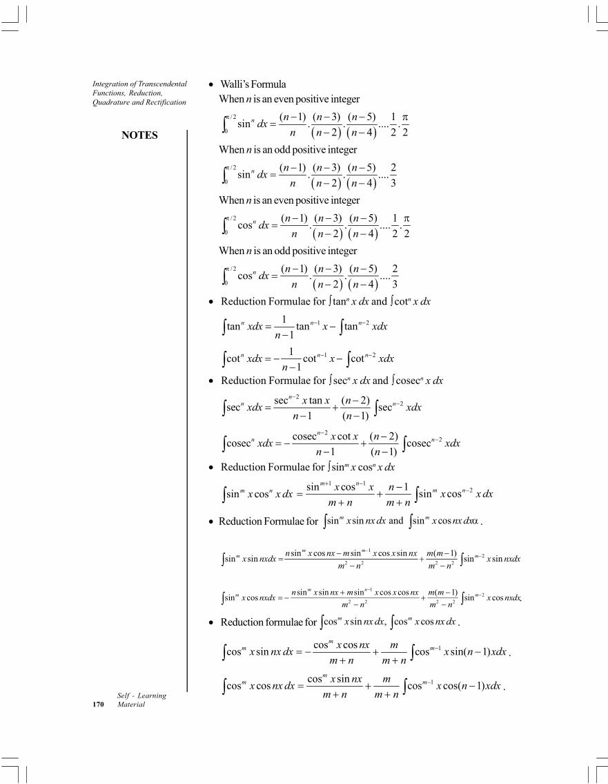
Integration of TranscendentalFunctions, Reduction,Quadrature and Rectification
NOTES
Self - Learning170 Material
Walli’s FormulaWhen n is an even positive integer
/ 2
0
( 1) ( 3) ( 5) 1sin . . .... .
2 4 2 2n n n n
dxn n n
When n is an odd positive integer
/ 2
0
( 1) ( 3) ( 5) 2sin . . ....
2 4 3n n n n
dxn n n
When n is an even positive integer
/ 2
0
( 1) ( 3) ( 5) 1cos . . .... .
2 4 2 2n n n n
dxn n n
When n is an odd positive integer
/ 2
0
( 1) ( 3) ( 5) 2cos . . ....
2 4 3n n n n
dxn n n
Reduction Formulae for tann x dx and cotn x dx
1 21tan tan tan
1n n nxdx x xdx
n
1 21
cot cot cot1
n n nxdx x xdxn
Reduction Formulae for secn x dx and cosecn x dx2
2sec tan ( 2)sec sec
1 ( 1)
nn nx x n
xdx xdxn n
22cosec cot ( 2)
cosec cosec1 ( 1)
nn nx x n
xdx xdxn n
Reduction Formulae for sinm x cosn x dx
sin cosm nx x dx1 1
2sin cos 1sin cos
m nm nx x n
x x dxm n m n
Reduction Formulae for sin sin and sin cosm mx nx dx x nx dx .
12
2 2 2 2
sin cos sin cos sin ( 1)sin sin sin sin
m mm mn x nx m x x nx m m
x nxdx x nxdxm n m n
12
2 2 2 2
sin sin sin cos cos ( 1)sin cos sin cos
m nm mn x nx m x x nx m m
x nxdx x nxdxm n m n
.
Reduction formulae for cos sin , cos cosm mx nx dx x nx dx .
1cos coscos sin cos sin( 1)
mm mx nx m
x nx dx x n xdxm n m n
.
1cos sincos cos cos cos( 1)
mm mx nx m
x nx dx x n xdxm n m n
.
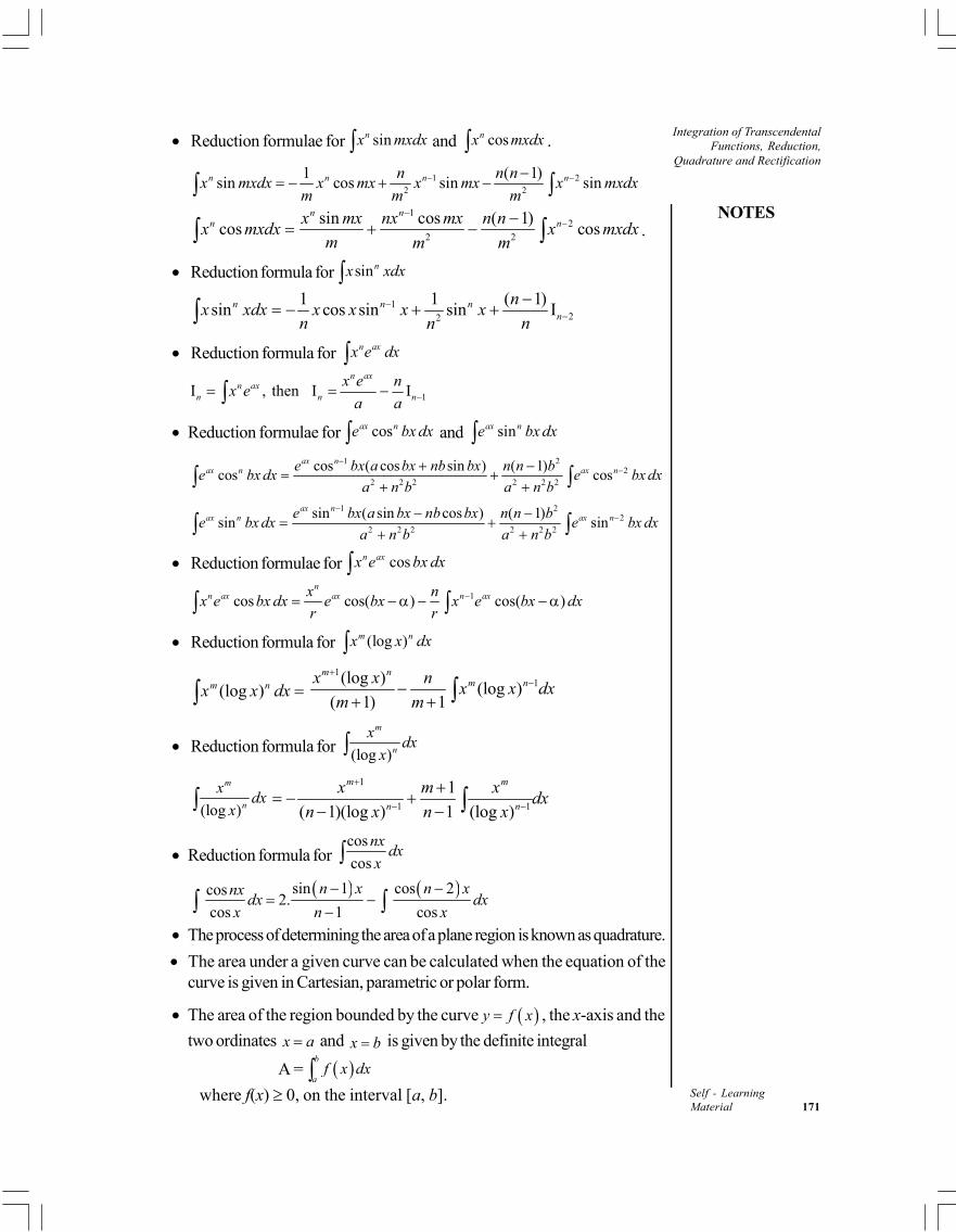
NOTES
Integration of TranscendentalFunctions, Reduction,
Quadrature and Rectification
Self - LearningMaterial 171
Reduction formulae for sinnx mxdx and cosnx mxdx .
1 22 2
1 ( 1)sin cos sin sinn n n nn n n
x mxdx x mx x mx x mxdxm m m
12
2 2
sin cos ( 1)cos cos
n nn nx mx nx mx n n
x mxdx x mxdxm m m
.
Reduction formula for sinnx xdx1
22
1 1 ( 1)sin cos sin sin In n n
n
nx xdx x x x x
n nn
Reduction formula for n axx e dx
1I , then I In ax
n axn n n
x e nx e
a a Reduction formulae for cosax ne bx dx and sinax ne bx dx
1 22
2 2 2 2 2 2
cos ( cos sin ) ( 1)cos cos
ax nax n ax ne bx a bx nb bx n n b
e bx dx e bx dxa n b a n b
1 22
2 2 2 2 2 2
sin ( sin cos ) ( 1)sin sin
ax nax n ax ne bx a bx nb bx n n b
e bx dx e bx dxa n b a n b
Reduction formulae for cosn axx e bx dx1cos cos( ) cos( )
nn ax ax n axx n
x e bx dx e bx x e bx dxr r
Reduction formula for (log )m nx x dx
(log )m nx x dx 1
1(log )(log )
( 1) 1
m nm nx x n
x x dxm m
Reduction formula for (log )
m
n
xdx
x
(log )
m
n
xdx
x1
1 1
1
( 1)(log ) 1 (log )
m m
n n
x m xdx
n x n x
Reduction formula for cos
cosnx
dxx
sin 1 cos 2cos2.
cos 1 cos
n x n xnxdx dx
x n x
The process of determining the area of a plane region is known as quadrature.
The area under a given curve can be calculated when the equation of thecurve is given in Cartesian, parametric or polar form.
The area of the region bounded by the curve y f x , the x-axis and the
two ordinates x a and x b is given by the definite integral
A = b
af x dx
where f(x) 0, on the interval [a, b].
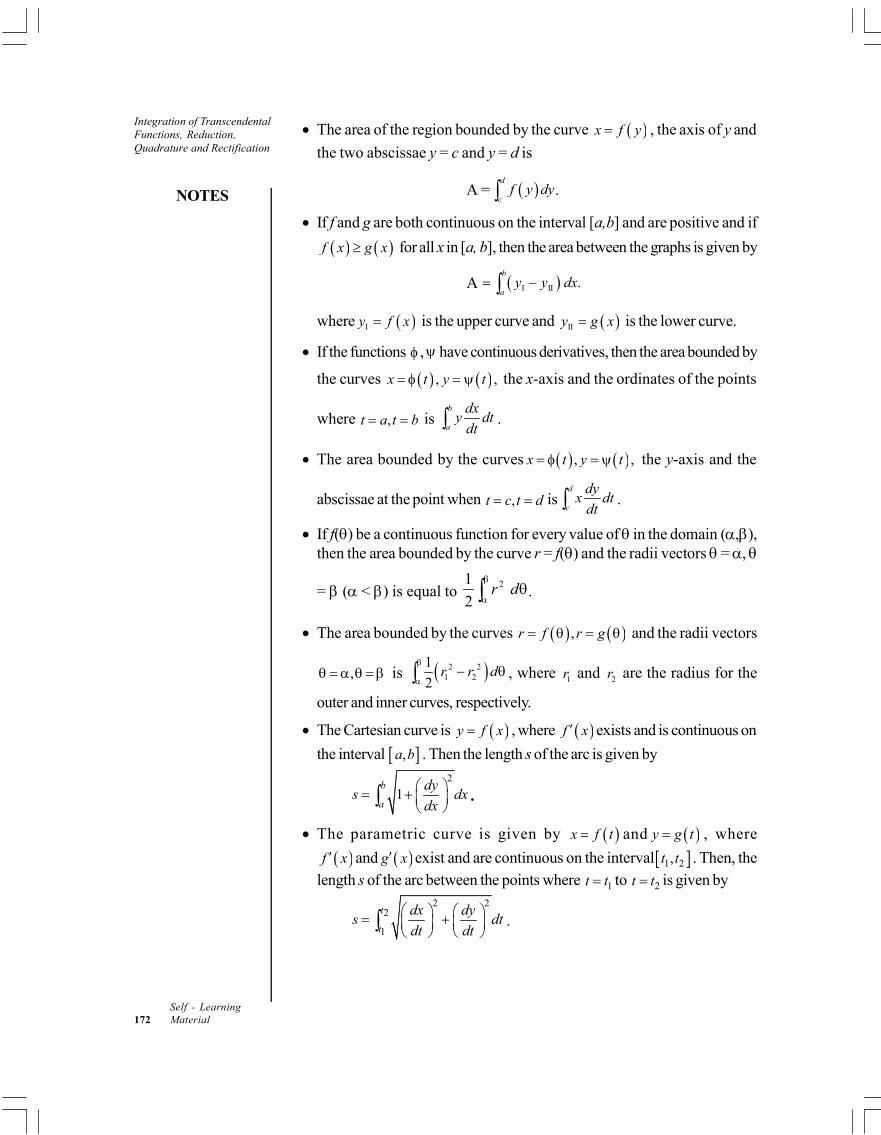
Integration of TranscendentalFunctions, Reduction,Quadrature and Rectification
NOTES
Self - Learning172 Material
The area of the region bounded by the curve x f y , the axis of y and
the two abscissae y = c and y = d is
A = d
cf y dy .
If f and g are both continuous on the interval [a,b] and are positive and if
f x g x for all x in [a, b], then the area between the graphs is given by
A I II .b
ay y dx
where Iy f x is the upper curve and IIy g x is the lower curve.
If the functions , have continuous derivatives, then the area bounded by
the curves , ,x t y t the x-axis and the ordinates of the points
where ,t a t b is b
a
dxy dt
dt .
The area bounded by the curves , ,x t y t the y-axis and the
abscissae at the point when ,t c t d isd
c
dyx dt
dt .
If f() be a continuous function for every value of in the domain (,),then the area bounded by the curve r = f() and the radii vectors = ,
= ( < ) is equal to 21
2r d
.
The area bounded by the curves ,r f r g and the radii vectors
, is 2 21 2
1
2r r d
, where 1r and 2r are the radius for the
outer and inner curves, respectively.
The Cartesian curve is y f x , where f x exists and is continuous on
the interval ,a b . Then the length s of the arc is given by
2
1b
a
dys dx
dx .
The parametric curve is given by x f t and y g t , where
f x and g x exist and are continuous on the interval 1 2,t t . Then, the
length s of the arc between the points where 1t t to 2t t is given by2 2
2
1
t
t
dx dys dt
dt dt .
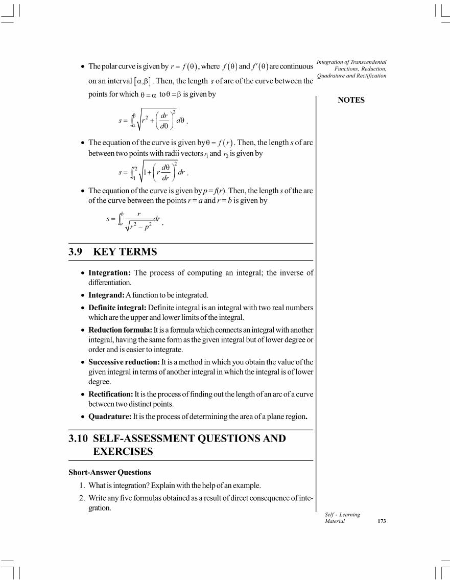
NOTES
Integration of TranscendentalFunctions, Reduction,
Quadrature and Rectification
Self - LearningMaterial 173
The polar curve is given by r f , where f and f are continuous
on an interval , . Then, the length s of arc of the curve between the
points for which to is given by
22 dr
s r dd
.
The equation of the curve is given by f r . Then, the length s of arcbetween two points with radii vectors 1r and 2r is given by
22
11
r
r
ds r dr
dr
.
The equation of the curve is given by p = f(r). Then, the length s of the arcof the curve between the points r = a and r = b is given by
2 2
b
a
rs dr
r p
.
3.9 KEY TERMS
Integration: The process of computing an integral; the inverse ofdifferentiation.
Integrand: A function to be integrated.
Definite integral: Definite integral is an integral with two real numberswhich are the upper and lower limits of the integral.
Reduction formula: It is a formula which connects an integral with anotherintegral, having the same form as the given integral but of lower degree ororder and is easier to integrate.
Successive reduction: It is a method in which you obtain the value of thegiven integral in terms of another integral in which the integral is of lowerdegree.
Rectification: It is the process of finding out the length of an arc of a curvebetween two distinct points.
Quadrature: It is the process of determining the area of a plane region.
3.10 SELF-ASSESSMENT QUESTIONS ANDEXERCISES
Short-Answer Questions
1. What is integration? Explain with the help of an example.
2. Write any five formulas obtained as a result of direct consequence of inte-gration.
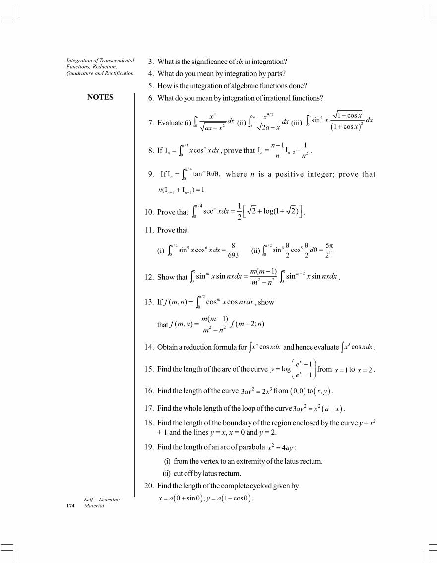
Integration of TranscendentalFunctions, Reduction,Quadrature and Rectification
NOTES
Self - Learning174 Material
3. What is the significance of dx in integration?
4. What do you mean by integration by parts?
5. How is the integration of algebraic functions done?
6. What do you mean by integration of irrational functions?
7. Evaluate (i) 0 2
na x
dxax x
(ii)9 / 2
2
0 2
a xdx
a x (iii) 4
20
1 cossin .
1 cos
xx dx
x
8. If / 2
0I cosn
n x x dx
, prove that 2 2
1 1I In n
n
n n
.
9. If/ 4
0I tan ,n
n d
where n is a positive integer; prove that
1 1(I I ) 1n nn
10. Prove that / 4 3
0
1sec 2 log(1 2)
2xdx
.
11. Prove that
(i) / 2 5 6
0
8sin cos
693x x dx
(ii)
/ 2 6 8110
5sin cos
2 2 2d
12. Show that2
2 20 0
( 1)sin sin sin sinm mm m
x nxdx x nxdxm n
.
13. If0
( , ) cos cosmf m n x nxdx
, show
that 2 2
( 1)( , ) ( 2; )
m mf m n f m n
m n
14. Obtain a reduction formula for cosnx xdx and hence evaluate 3 cosx xdx .
15. Find the length of the arc of the curve 1
log1
x
x
ey
e
from 1x to 2x .
16. Find the length of the curve 2 33 2ay x from 0,0 to ,x y .
17. Find the whole length of the loop of the curve 2 23ay x a x .
18. Find the length of the boundary of the region enclosed by the curve y = x2
+ 1 and the lines y = x, x = 0 and y = 2.
19. Find the length of an arc of parabola 2 4x ay :
(i) from the vertex to an extremity of the latus rectum.
(ii) cut off by latus rectum.
20. Find the length of the complete cycloid given by
sin , 1 cosx a y a .
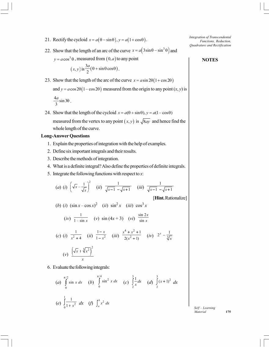
NOTES
Integration of TranscendentalFunctions, Reduction,
Quadrature and Rectification
Self - LearningMaterial 175
21. Rectify the cycloid sin , 1 cosx a y a .
22. Show that the length of an arc of the curve 33sin sinx a and3cosy a , measured from 0,a to any point
,x y is 3sin cos
2
a .
23. Show that the length of the arc of the curve sin 2 1 cos 2x a
and cos2 1 cos2y a measured from the origin to any point (x, y) is
4sin 3
3
a .
24. Show that the length of the cycloid ( sin ), (1 cos )x a y a
measured from the vertex to any point ,x y is 8ay and hence find the
whole length of the curve.
Long-Answer Questions
1. Explain the properties of integration with the help of examples.
2. Define six important integrals and their results.
3. Describe the methods of integration.
4. What is a definite integral? Also define the properties of definite integrals.
5. Integrate the following functions with respect to x:
(a) (i)2
1–x
x(ii)
1
1 1x x (iii)1
1 1x x
[Hint. Rationalize]
(b) (i) (sin x – cos x)2 (ii) sin2 x (iii) cos3 x
(iv)1
1 sin x (v) sin (4x + 3) (vi)sin 2
sin
x
x
(c) (i) 2
1
4x (ii) 2
1
1
x
x (iii)4 2
2
1
2( 1)
x x
x(iv) 3
12x
x
(v)
23 2x x
x
6. Evaluate the following integrals:
(a)π /2
0
sin x dx (b)π/4
2
0
sin x dx (c)3
2
1dx
x (d)3
2
2
( 1)x dx
(e)1
20
1
1 x dx (f) 2b
ax dx
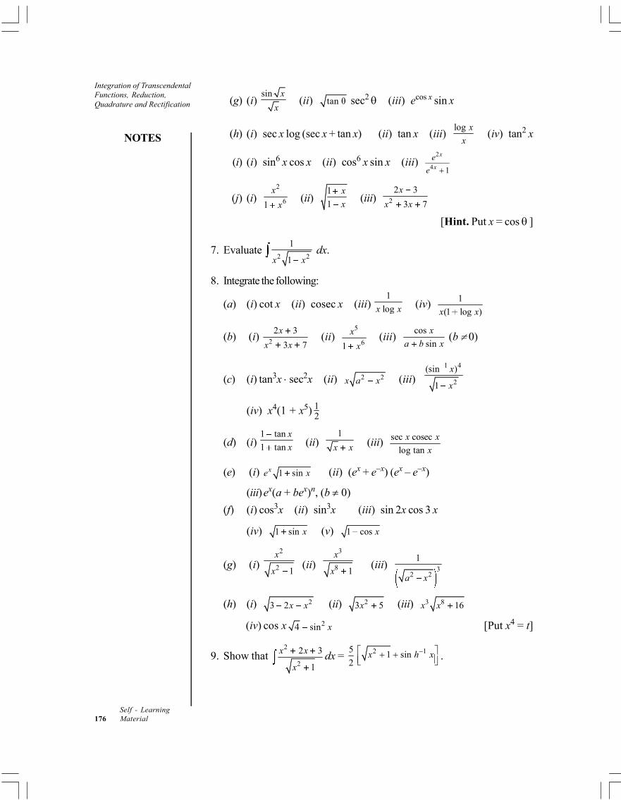
Integration of TranscendentalFunctions, Reduction,Quadrature and Rectification
NOTES
Self - Learning176 Material
(g) (i) sin x
x(ii) tan θ sec2 (iii) ecos x sin x
(h) (i) sec x log (sec x + tan x) (ii) tan x (iii)log x
x(iv) tan2 x
(i) (i) sin6 x cos x (ii) cos6 x sin x (iii)2
4 1
x
x
e
e
(j) (i)2
61
x
x(ii)
1
1
x
x(iii) 2
2 3
3 7
x
x x
[Hint. Put x = cos ]
7. Evaluate 2 2
1
1x x dx.
8. Integrate the following:
(a) (i) cot x (ii) cosec x (iii) 1
logx x (iv) 1
(1 log )x x
(b) (i) 2
2 3
3 7
x
x x(ii)
5
61
x
x(iii)
cos
sin
x
a b x (b 0)
(c) (i) tan3x sec2x (ii) 2 2x a x (iii) 1 4
2
(sin )
1
x
x
(iv) x4(1 + x5) 12
(d) (i) 1 tan
1 tan
x
x (ii)1
x x (iii) sec cosec
log tan
x x
x
(e) (i) 1 sinxe x (ii) (ex + e–x) (ex – e–x)
(iii)ex(a + bex)n, (b 0)
(f) (i) cos3x (ii) sin3x (iii) sin 2x cos 3 x
(iv) 1 sin x (v) 1 cos x
(g) (i) 2
2 1
x
x(ii)
3
8 1
x
x (iii) 3
2 2
1
a x
(h) (i) 23 2x x (ii) 23 5x (iii) 3 8 16x x
(iv) cos x 24 sin x [Put x4 = t]
9. Show that 2
2
2 3
1
x x
xdx =
5
22 11 sinx h x .
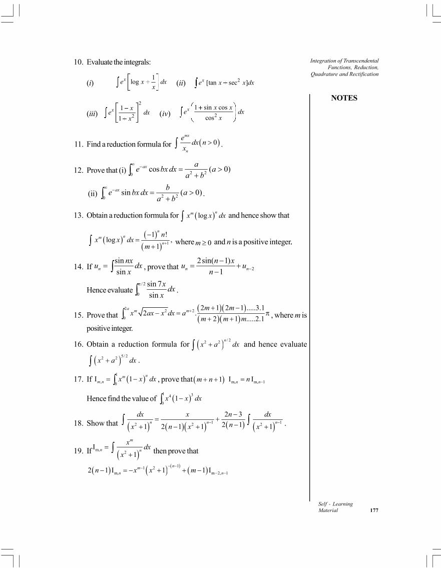
NOTES
Integration of TranscendentalFunctions, Reduction,
Quadrature and Rectification
Self - LearningMaterial 177
10. Evaluate the integrals:
(i)1
logxe x dxx (ii) 2[tan sec ]xe x x dx
(iii)
2
2
1
1x x
e dxx
(iv) 2
1 sin cos
cosx x x
e dxx
11. Find a reduction formula for 0mx
n
edx n
x .
12. Prove that (i) 2 20cos ( 0)ax a
e bx dx aa b
(ii) 2 20sin ( 0)ax b
e bx dx aa b
.
13. Obtain a reduction formula for lognmx x dx and hence show that
1
1 !log ,
1
nnm
n
nx x dx
m
where 0m and n is a positive integer..
14. If sin
sinn
nxu dx
x , prove that 2
2sin( 1)
1n n
n xu u
n
Hence evaluate/ 2
0
sin 7
sin
xdx
x
.
15. Prove that
2 2 2
0
2 1 2 1 .....3.12 .
2 1 .....2.1
a m m m mx ax x dx a
m m m
, where m is
positive integer.
16. Obtain a reduction formula for / 22 2 nx a dx and hence evaluate
5/ 22 2x a dx .
17. If 1
, 0I 1
nmm n x x dx , prove that 1m n m, m, 1I In nn
Hence find the value of 1 34
01x x dx
18. Show that 1 12 2 2
2 3
2 11 2 1 1 1n n n
dx x n dx
nx n x x
.
19. If m,2
I1
m
n n
xdx
x
then prove that
11 2m, m 2, 12 1 I 1 1 I
nmn nn x x m
Integration of TranscendentalFunctions, Reduction,Quadrature and Rectification
NOTES
Self - Learning178 Material
20. Find the whole area of the curve 2
2 2
1 2, .
1 1
t atx a y
t t
21. Show that the area of a loop of the curve 3 cos3 sin3r is 3
.
22. Show that the area contained between the circle r = a and the curvecos5r a is equal to three-fourths of the area of the circle.
23. Find the area inside the circle sinr and outside the cardioid
1 cosr .
24. Find the area outside the circle 2 cosr a and inside the cardioid
1 cosr a .
3.11 FURTHER READING
Prasad, Gorakh. 2016. Differential Calculus. Allahabad: Pothishala Private Ltd.
Prasad, Gorakh. 2015. Integral Calculus. Allahabad: Pothishala Private Ltd.
Murray, Daniel A. 1967. Introductory Course in Differential Equations. India:Orient Longman.
Coddington, Earl A. 1987. An Introduction to Ordinary Differential Equations.New Delhi: Prentice Hall of India.
Coddington, Earl A. and N. Levinson. 1972. Theory of Ordinary DifferentialEquations. New Delhi: Tata Mc Graw-Hill.
Boyce, W.E. and Richard C. DiPrima. 1986. Elementary Differential Equationsand Boundary Value Problems. New York: John Wiley and Sons, Inc.
Gelfand, J.M. and S.V. Fomin. 1963. Calculus of Variations. New Jersey: PrenticeHall.
Ross, S. L. 1984. Differential Equations, 3rd Edition. New York: John Wileyand Sons.
Somasundaram, D. 2002. Ordinary Differential Equations. Chennai: NarosaPublishing House.
NOTES
Differential Equations
Self - LearningMaterial 179
UNIT 4 DIFFERENTIAL EQUATIONS
Structure
4.0 Introduction4.1 Objectives4.2 Linear Differential Equations
4.2.1 Geometrical Meaning of a Differential Equation4.2.2 Solving Linear Differential Equations
4.3 Equations Reducible to the Linear Form4.4 Exact Differential Equations4.5 First Order Higher Degree Equations Solvable for x, y and p4.6 Clairaut’s Equation4.7 Singular Solutions4.8 Orthogonal Trajectories4.9 Answers to ‘Check Your Progress’
4.10 Summary4.11 Key Terms4.12 Self-Assessment Questions and Exercises4.13 Further Reading
4.0 INTRODUCTION
In mathematics, a Differential Equation (DE) is defined as an equation of the formthat interconnects certain function with its derivatives, where usually the functionrepresents the physical quantity while the derivatives denote their rates of changeand the relationship between the two is defined by the equation. Fundamentally,the ‘solutions of differential equations’ are functions which precisely ‘represent therelationship or correlation between a continuously varying or fluctuating quantityand its rate of change’. A Differential Equation (DE) comprises of one or moreexpressions including derivatives of one dependent variable ‘y’ with reference toanother independent variable ‘x’. An ordinary differential equation is a differentialequation that includes a function of a single variable and some of its derivatives.Principally, a differential equation is an equation for a function that relates thevalues of the function to the values of its derivatives. Therefore, a differential equationis an equation between specified derivative on an unknown function, its values andknown quantities and functions or a Differential Equation (DE) is an equation thatcomprises of a function and its derivatives. Differential equations are categorizedas Partial Differential Equations (PDE) or Ordinary Differential Equations (ODE)in accordance with whether or not they hold partial derivatives, while the order ofa differential equation is defined on the basis of the highest order derivative thatoccurs in the equation.
Differential Equations
NOTES
Self - Learning180 Material
In mathematics, a linear differential equation is a differential equation that isdefined by a linear polynomial in the unknown function and its derivatives, that isan equation of the form,
0 1 2 0nna x y a x y a x y a x y b x
where a0(x), ..., a
n(x) and b(x) are arbitrary differentiable functions that do not
essential to be linear, and y, …, y (n) are considered as the successive derivativesof an unknown function y of the variable x. A linear differential equation may alsobe a Linear Partial Differential Equation (Linear PDE), if the unknown functiondepends on several variables, and the derivatives that appear in the equation arepartial derivatives. If a linear differential equation or a system of linear equationsare such that the associated homogeneous equations have constant coefficientsthen these may be solved by means of quadrature mathematics, i.e., the solutionsmay be expressed in terms of integrals. This is also true for a linear equation oforder one with non-constant coefficients.
By a differential equation, you mean an equation which involves derivatives of adependent variable with respect to one or more independent variables. Some
examples of differential equations are 6dy
xdx
, 2
25 8 0
d y dyy
dx dx and
2 22
2 2
z zx y
x y
. Symbolically, a differential equation can be written
as2
2, , , ,...,
n
n
dy d y d yf x y
dx dx dx
. There are two types of differential equations: ordinary
differential equations and partial differential equations. Ordinary differentialequations involve only one independent variable, while the partial differentialequations involve the partial derivatives with respect to two or more independentvariables. In this unit, you will learn about only ordinary differential equations,including the necessary conditions for an ordinary differential equation to be exact.
The first order differential equations are used to formulate the problem offinding the other parameter family of curves, which is orthogonal to the givenparameter family of curves.
In this unit, you will study about the linear differential equations and equationsreducible to the linear form, exact differential equations, first order higher degreeequations solvable for x, y and p, Clairaut’s equation and singular solutions,geometrical meaning of a differential equation, and orthogonal trajectories.
4.1 OBJECTIVES
After going through this unit, you will be able to:
Give the geometrical meaning of differential equations
Know the necessary and sufficient condition required for an ordinarydifferential equation to be exact, i.e., exact differential equations
NOTES
Differential Equations
Self - LearningMaterial 181
Find the solution of a given differential equation
Elaborate on the linear differential equations and equations reducible to thelinear form
Find integrating factor of an equation by inspection method and using variousrules
Define differential equation of first order and higher degree
Solve the first order higher degree differential equations solvable for x, yand p
Understand Clairaut’s equation and singular solutions
Find the singular solution of a first order higher degree differential equation
Define p-discriminant and c-discriminant forms
Understand the meaning of trajectory and orthogonal trajectories
Derive and apply differential equations of orthogonal trajectories in Cartesianand polar co-ordinates
4.2 LINEAR DIFFERENTIAL EQUATIONS
In mathematics, a Differential Equation (DE) is defined as an equation of theform that interconnects certain function with its derivatives, where usually the functionrepresents the physical quantity while the derivatives denote their rates of changeand the relationship between the two is defined by the equation. Fundamentally,the ‘solutions of differential equations’ are functions which precisely ‘representthe relationship or correlation between a continuously varying or fluctuating quantityand its rate of change’.
A Differential Equation (DE) comprises of one or more expressions includingderivatives of one dependent variable ‘y’ with reference to another independentvariable ‘x’, such as
2dy
xdx
An ordinary differential equation is a differential equation that includes afunction of a single variable and some of its derivatives, such as
22 3 5dy
x xdx
Principally, a differential equation is an equation for a function that relatesthe values of the function to the values of its derivatives. Therefore, a differentialequation is an equation between specified derivative of an unknown function, itsvalues and known quantities and functions or a Differential Equation (DE) is anequation that comprises of a function and its derivatives. Differential equations arecategorized as Partial Differential Equations (PDE) or Ordinary DifferentialEquations (ODE) in accordance with whether or not they hold partial derivatives,
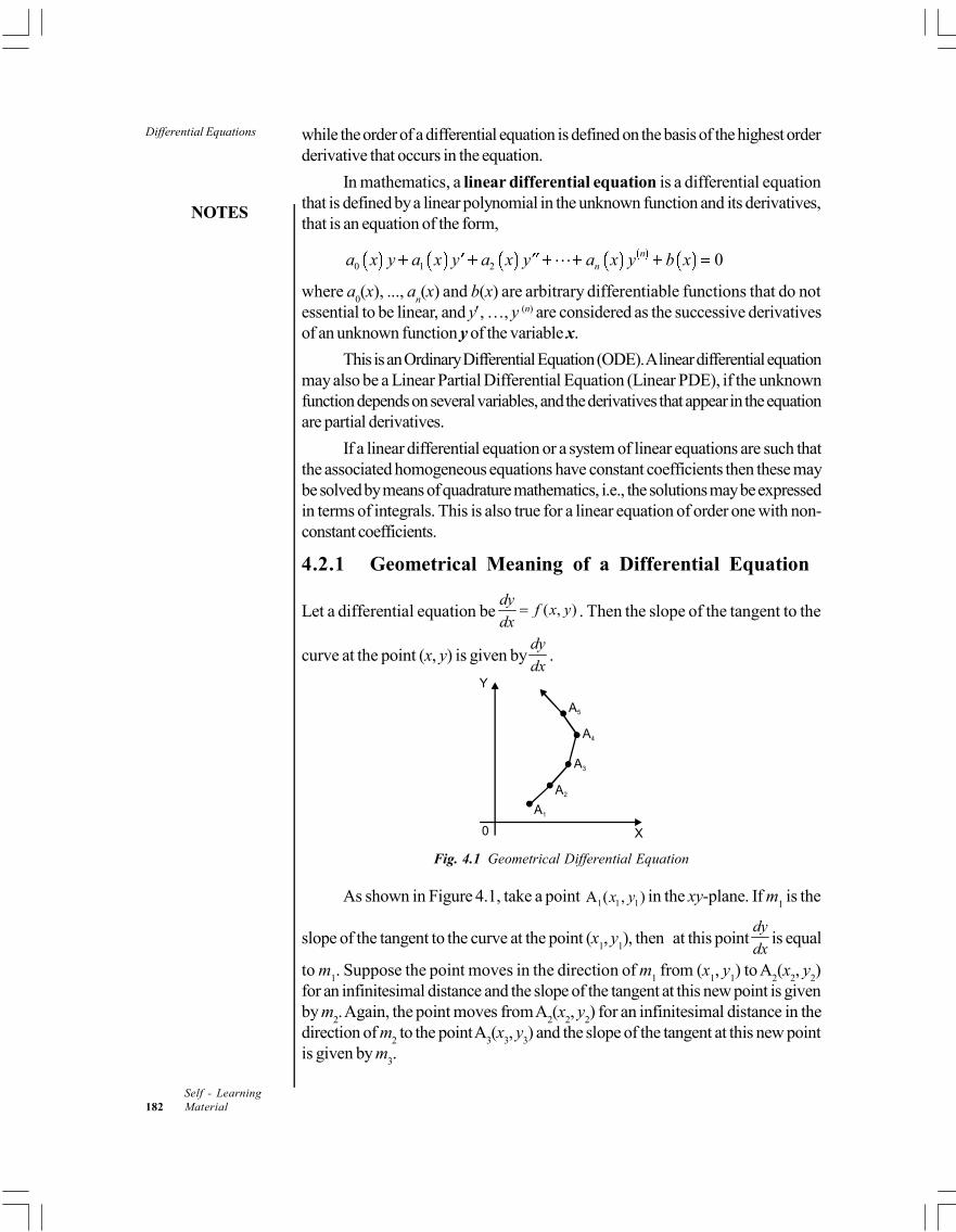
Differential Equations
NOTES
Self - Learning182 Material
while the order of a differential equation is defined on the basis of the highest orderderivative that occurs in the equation.
In mathematics, a linear differential equation is a differential equationthat is defined by a linear polynomial in the unknown function and its derivatives,that is an equation of the form,
0 1 2 0 nna x y a x y a x y a x y b x
where a0(x), ..., a
n(x) and b(x) are arbitrary differentiable functions that do not
essential to be linear, and y, …, y (n) are considered as the successive derivativesof an unknown function y of the variable x.
This is an Ordinary Differential Equation (ODE). A linear differential equationmay also be a Linear Partial Differential Equation (Linear PDE), if the unknownfunction depends on several variables, and the derivatives that appear in the equationare partial derivatives.
If a linear differential equation or a system of linear equations are such thatthe associated homogeneous equations have constant coefficients then these maybe solved by means of quadrature mathematics, i.e., the solutions may be expressedin terms of integrals. This is also true for a linear equation of order one with non-constant coefficients.
4.2.1 Geometrical Meaning of a Differential Equation
Let a differential equation be ( , )dy
f x ydx
. Then the slope of the tangent to the
curve at the point (x, y) is given bydy
dx.
A1
A2
A3
A4
A5
Y
X0
Fig. 4.1 Geometrical Differential Equation
As shown in Figure 4.1, take a point 1 1 1A ( , )x y in the xy-plane. If m1 is the
slope of the tangent to the curve at the point (x1, y
1), then at this point
dy
dxis equal
to m1. Suppose the point moves in the direction of m
1 from (x
1, y
1) to A
2(x
2, y
2)
for an infinitesimal distance and the slope of the tangent at this new point is givenby m
2. Again, the point moves from A
2(x
2, y
2) for an infinitesimal distance in the
direction of m2 to the point A
3(x
3, y
3) and the slope of the tangent at this new point
is given by m3.
NOTES
Differential Equations
Self - LearningMaterial 183
Choosing the successive points A1, A
2, A
3, … near to the one another
makes the broken curve approximate to a smooth curve ( )y x which is
associated with the initial point 1 1 1A ( , )x y . The slope of the tangent to the curve at
a point and the co-ordinate of that point always satisfy the equation ( , )dy
f x ydx
.
On choosing different initial points, different curves with the same property
will be obtained. Thus, we can say that the differential equation ( , )dy
f x ydx
represents a family of curves such that through each point of the xy-plane, therepasses one curve of the family.
4.2.2 Solving Linear Differential Equations
The linear differential equation is a differential equation in which the dependentvariable and all its derivatives appear only in the first degree and are not multipliedtogether.
A linear differential equation of order n is of the form
1 2
0 1 21 2P P P ....... P X
n n n
nn n n
d y d y d yy
dx dx dx
… (1)
where, P0, P
1, P
2,….., P
n and X are either the functions of x or constants.
When in Equation (1), P0, P
1, P
2,…, P
n are all constants and not the function
of x while X is the some function of x, the equation is called a linear differentialequation with constant co-efficients of nth order.
Differential Operator ‘D’
Sometimes, it is easier to write a linear differential equation in the simple form by
replacing the part d
dx of the symbol
dy
dxwith D. This D or
d
dxis regarded as
differential operator.
So, Equation (1) can be written in terms of differential operator D as
1 20 1 2P D P D P D ....... P Xn n n
n y
Or f(D)y = X where f(D) = 1 20 1 2P D P D P D ....... Pn n n
n .
Solution of Linear Differential Equations
Theorem 4.1: If y = y1, y = y
2, …, y = y
n be the linear independent solutions of
1 20 1 2D D D ....... 0n n n
na a a a y , then 1 1 2 2 .... n ny c y c y c y
where c1, c
2, c
3, ...,c
n are arbitrary constants, is the general or complete solution
of the differential Equation (1).
Proof: Given, 1 20 1 2D D D ....... 0n n n
na y a y a y a y … (2)
Differential Equations
NOTES
Self - Learning184 Material
As y = y1, y = y
2,…, y = y
n are solutions of Equation (2),
1 20 1 1 1 2 1 1D D D ....... 0n n n
na y a y a y a y 1 2
0 2 1 2 2 2 2D D D ....... 0n n nna y a y a y a y
………………………………………………… …………………………………………………… ……………………………………………………
1 20 1 2D D D ....... 0n n n
n n n n na y a y a y a y
1 1 2 2 .... n ny c y c y c y
… (3)
Now, by putting 1 1 2 2 .... n ny c y c y c y in Equation (2), we get
10 1 1 2 2 1 1 1 2 2
1 1 2 2
D ... D ...
.................................... ... 0
n nn n n n
n n n
a c y c y c y a c y c y c y
a c y c y c y
1 11 0 1 1 1 1 2 0 2 1 2 2
10 1
D D ..... D D .....
.................................... D D ..... 0
n n n nn n
n nn n n n n
c a y a y a y c a y a y a y
c a y a y a y
Substituting the values from Equation (3) in the above equation, we get
c1.0 + c
2.0 + ... + c
n.0 = 0 0 = 0
Thus, 1 1 2 2 .... n ny c y c y c y satisfies the Equation (2), which istherefore its solution.
Auxiliary Equation
Consider 1 20 1 2D D D ....... 0n n n
na y a y a y a y … (4)
where, a0, a
1, a
2, ...,a
n are all constants.
Now, let one of the solution of Equation (4) be mxy e .
Then, D mxy me , 2 2D mxy m e ,…, Dn n mxy m e
By putting all these values including mxy e in Equation (4), we get
1 20 1 2 ....... 0n n n mx
na m a m a m a e
Since, 0mxe for any m, therefore,
1 20 1 2 ....... 0n n n
na m a m a m a … (5)
This equation in m is known as auxiliary equation of the given differentialEquation (4).
If m is a solution of Equation (5), then emx will be a solution of Equation (4).To solve the Equation (4), write its auxiliary equation and then solve it first.
NOTES
Differential Equations
Self - LearningMaterial 185
Note: The values of D obtained from
1 20 1 2(D) D D D ....... 0n n n
nf a a a a … (6)
is same as the values of m obtained from Equation (5). Hence, Equation (6), ingeneral can be regarded as the auxiliary equation which is obtained by equatingthe symbolic coefficient of y in Equation (4) to zero. Thus, in practice we do notreplace D by m to form an auxiliary equation.
The roots of the auxiliary equation can be as follows:
Real and Different
Real and Repeated
Complex
Case I: When all the roots of Equation (5) are real and different.
Let 1 2 3, , , ....... nm m m m be the n different and real roots of Equation (5).Then
31 2, , ,...,m x m xm x m x ne e e e will be the n distinct solutions of Equation (4).
Thus, the general solution of Equation (4) is
31 21 2 3 .....m x m xm x m x n
ny c e c e c e c e … (7)
where c1, c
2,…, c
n are arbitrary constants.
Case II: When all the roots of Equation (5) are real, two of them are repeatedand all others are different.
Let 1m and 2m be the two equal roots of the auxiliary equation.
Then, Equation (7) becomes 311 2 3 .....m x m xm x n
ny c c e c e c e
which has only (n – 1) arbitrary constants and so it is no longer a generalsolution.
Consider a differential equation of second order
1 1D D 0m m y …(8)
whose auxiliary equation 21D 0m has equal roots.
Now, putting 1D m y = v in the Equation (8), we get
1D 0m v 1dv
m vdx
1dv
m dxv
On integrating both sides, we get
1log logv m x c
1m xv ce 11D m xm y ce 1
1m xdy
m y cedx
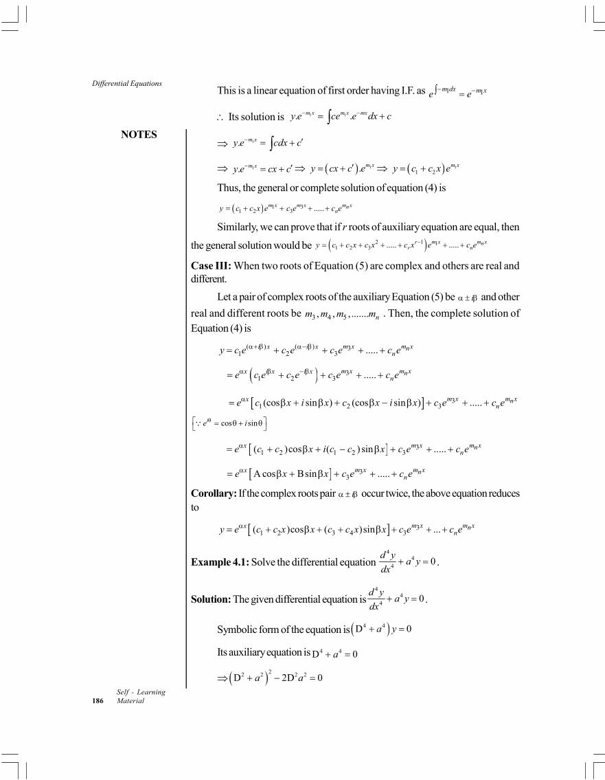
Differential Equations
NOTES
Self - Learning186 Material
This is a linear equation of first order having I.F. as 1 1m dx m xe e
Its solution is 1 1. .m x m x mxy e ce e dx c
1. m xy e cdx c 1. m xy e cx c 1. m xy cx c e 1
1 2m xy c c x e
Thus, the general or complete solution of equation (4) is
311 2 3 .....m x m xm x n
ny c c x e c e c e
Similarly, we can prove that if r roots of auxiliary equation are equal, then
the general solution would be 2 1 11 2 3 ..... ..... m xm xr n
r ny c c x c x c x e c e
Case III: When two roots of Equation (5) are complex and others are real anddifferent.
Let a pair of complex roots of the auxiliary Equation (5) be i and other
real and different roots be 3 4 5, , , ....... nm m m m . Then, the complete solution ofEquation (4) is
( ) ( ) 31 2 3 .....m x m xi x i x n
ny c e c e c e c e
31 2 3 .....m x m xx i x i x n
ne c e c e c e c e
31 2 3(cos sin ) (cos sin ) .....m x m xx n
ne c x i x c x i x c e c e
cos sinie i
31 2 1 2 3( )cos ( ) sin .....m x m xx n
ne c c x i c c x c e c e
33A cos Bsin .....m x m xx n
ne x x c e c e
Corollary: If the complex roots pair i occur twice, the above equation reducesto
31 2 3 4 3( )cos ( )sin ...m x m xx n
ny e c c x x c c x x c e c e
Example 4.1: Solve the differential equation 4
44
0d y
a ydx
.
Solution: The given differential equation is4
44
0d y
a ydx
.
Symbolic form of the equation is 4 4D 0a y
Its auxiliary equation is 4 4D 0a
22 2 2 2D 2D 0a a
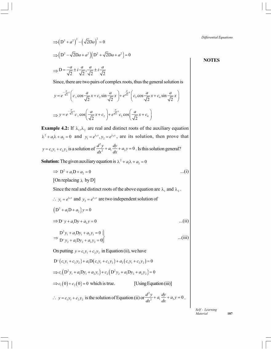
NOTES
Differential Equations
Self - LearningMaterial 187
222 2D 2D 0a a
2 2 2 2D 2D D 2D 0a a a a
D ,2 2 2 2
a a a ai i
Since, there are two pairs of complex roots, thus the general solution is
2 21 2 3 4cos sin cos sin
2 2 2 2
a ax xa a a a
y e c x c x e c x c x
2 21 2 3 4cos cos
2 2
a ax xa a
y e c x c e c x c
Example 4.2: If 1 2, are real and distinct roots of the auxiliary equation2
1 2 0a a and 1 21 2,x xy e y e , are its solution, then prove that
1 1 2 2y c y c y is a solution of 2
1 220
d y dya a y
dx dx . Is this solution general?
Solution: The given auxiliary equation is 21 2 0a a
21 2D D 0a a ...(i)
[On replacing by D]
Since the real and distinct roots of the above equation are 1 and 2 .
11
xy e and 22
xy e are two independent solution of
21 2D D 0a a y
21 2D D 0y a y a y ...(ii)
2
21 1 1 2 1
2 1 2 2 2
D D 0
D D 0
y a y a y
y a y a y
...(iii)
On putting 1 1 2 2y c y c y in Equation (ii), we have
21 1 2 2 1 1 1 2 2 2 1 1 2 2D D 0c y c y a c y c y a c y c y
2 21 1 1 1 2 1 2 2 1 2 2 2D D D D 0c y a y a y c y a y a y
1 20 0 0c c which is true. [Using Equation (iii)]
1 1 2 2y c y c y is the solution of Equation (ii) or2
1 220
d y dya a y
dx dx .
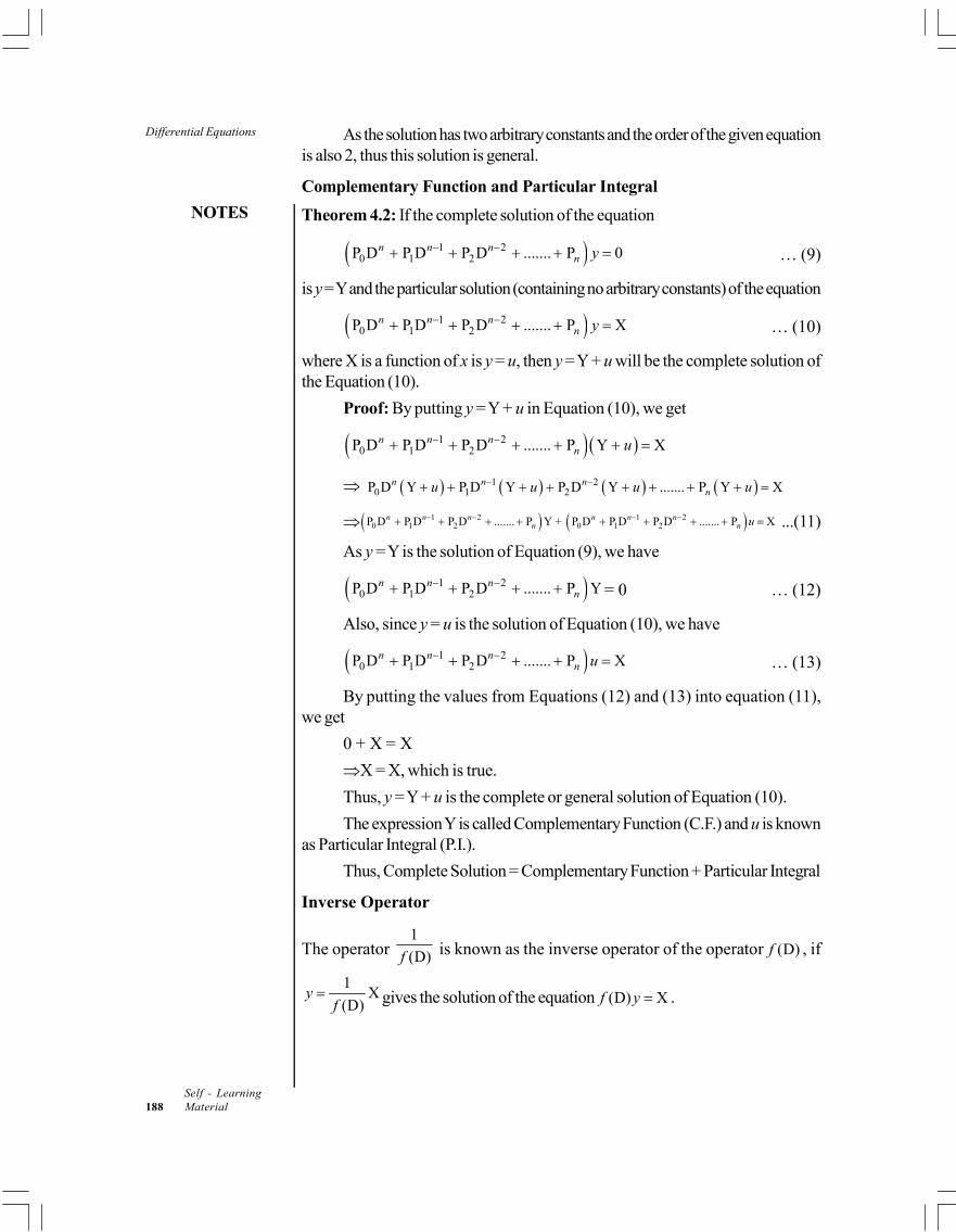
Differential Equations
NOTES
Self - Learning188 Material
As the solution has two arbitrary constants and the order of the given equationis also 2, thus this solution is general.
Complementary Function and Particular Integral
Theorem 4.2: If the complete solution of the equation
1 20 1 2P D P D P D ....... P 0n n n
n y … (9)
is y = Y and the particular solution (containing no arbitrary constants) of the equation
1 20 1 2P D P D P D ....... P Xn n n
n y … (10)
where X is a function of x is y = u, then y = Y + u will be the complete solution ofthe Equation (10).
Proof: By putting y = Y + u in Equation (10), we get
1 20 1 2P D P D P D ....... P Y Xn n n
n u
1 20 1 2P D Y P D Y P D Y ....... P Y Xn n n
nu u u u
1 2 1 20 1 2 0 1 2P D P D P D ....... P Y + P D P D P D ....... P Xn n n n n n
n n u ...(11)
As y = Y is the solution of Equation (9), we have
1 20 1 2P D P D P D ....... P Yn n n
n = 0 … (12)
Also, since y = u is the solution of Equation (10), we have
1 20 1 2P D P D P D ....... P Xn n n
n u … (13)
By putting the values from Equations (12) and (13) into equation (11),we get
0 + X = X
X = X, which is true.
Thus, y = Y + u is the complete or general solution of Equation (10).
The expression Y is called Complementary Function (C.F.) and u is knownas Particular Integral (P.I.).
Thus, Complete Solution = Complementary Function + Particular Integral
Inverse Operator
The operator 1
(D)f is known as the inverse operator of the operator (D)f , if
1X
(D)y
f gives the solution of the equation (D) Xf y .
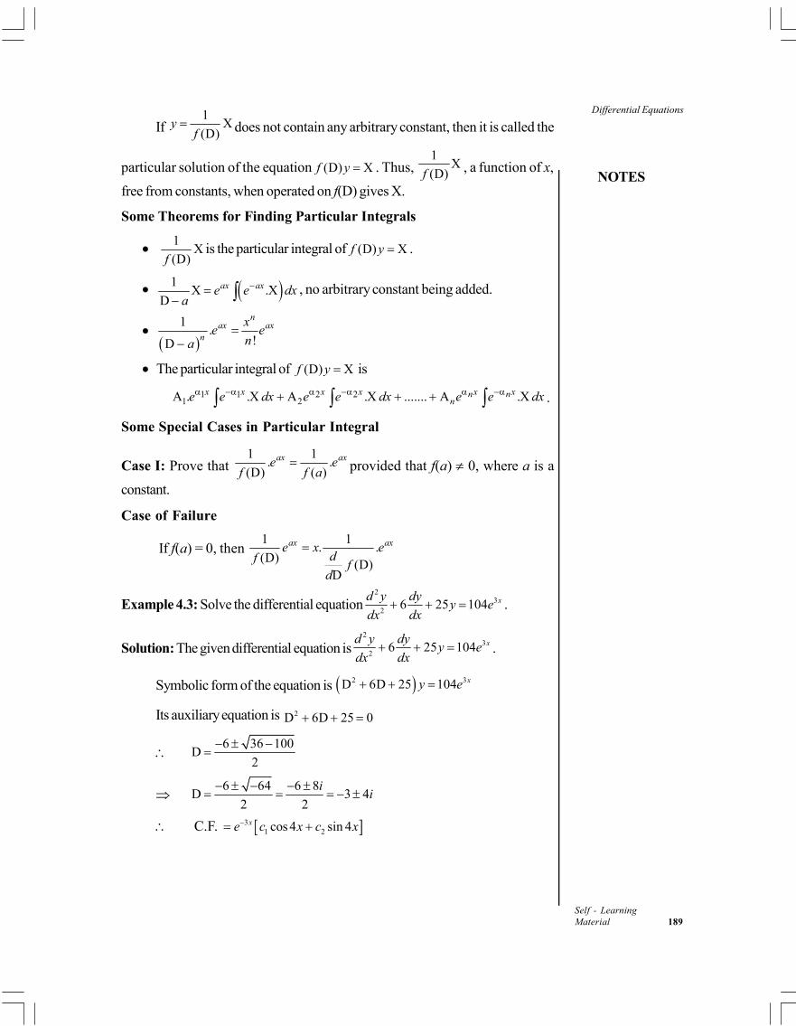
NOTES
Differential Equations
Self - LearningMaterial 189
If 1
X(D)
yf
does not contain any arbitrary constant, then it is called the
particular solution of the equation (D) Xf y . Thus, 1
X(D)f , a function of x,
free from constants, when operated on f(D) gives X.
Some Theorems for Finding Particular Integrals
1
X(D)f
is the particular integral of (D) Xf y .
1X .X
Dax axe e dx
a
, no arbitrary constant being added.
1.
!D
nax ax
n
xe e
na
The particular integral of (D) Xf y is
1 1 2 21 2A . .X A .X ....... A .Xx xx x x x n n
ne e dx e e dx e e dx .
Some Special Cases in Particular Integral
Case I: Prove that 1 1
. .(D) ( )
ax axe ef f a
provided that f(a) 0, where a is a
constant.
Case of Failure
If f(a) = 0, then 1 1
. .(D) (D)
D
ax axe x edf f
d
Example 4.3: Solve the differential equation2
32
6 25 104 xd y dyy e
dx dx .
Solution: The given differential equation is2
32
6 25 104 xd y dyy e
dx dx .
Symbolic form of the equation is 2 3D 6D 25 104 xy e
Its auxiliary equation is 2D 6D 25 0
6 36 100
D2
6 64 6 8
D 3 42 2
ii
C.F. 31 2cos 4 sin 4xe c x c x
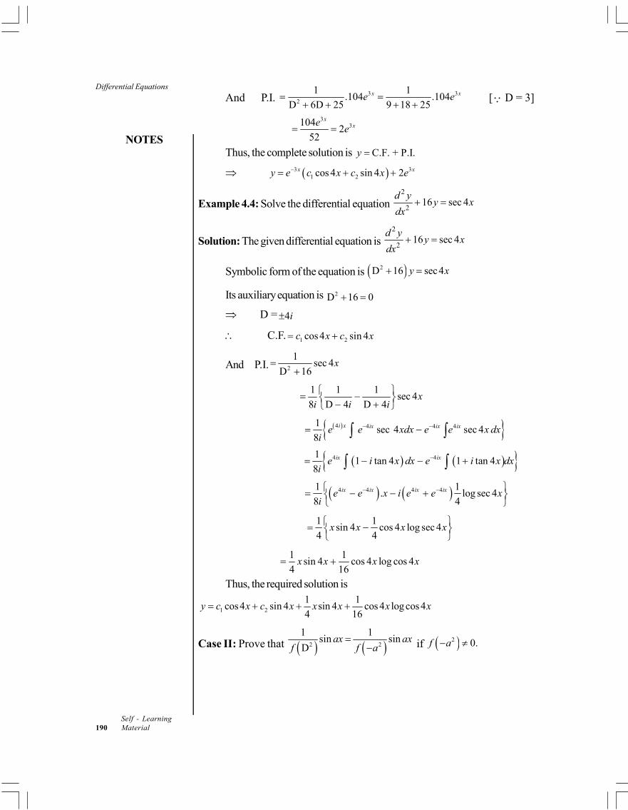
Differential Equations
NOTES
Self - Learning190 Material
And P.I. 3 32
1 1.104 .104
D 6D 25 9 18 25x xe e
[ D = 3]
3
31042
52
xxe
e
Thus, the complete solution is C.F. + P.I.y
3 31 2cos 4 sin 4 2x xy e c x c x e
Example 4.4: Solve the differential equation 2
216 sec 4
d yy x
dx
Solution: The given differential equation is 2
216 sec 4
d yy x
dx
Symbolic form of the equation is 2D 16 sec4y x
Its auxiliary equation is 2D 16 0
D = 4i
C.F. 1 2cos4 sin 4c x c x
And P.I. 2
1sec 4
D 16x
1 1 1
sec 48 D 4 D 4
xi i i
4 4 4 41sec 4 sec 4
8i x ix ix ixe e xdx e e x dx
i
4 411 tan 4 1 tan 4
8ix ixe i x dx e i x dx
i
4 4 4 41 1. log sec 4
8 4ix ix ix ixe e x i e e x
i
1 1
sin 4 cos 4 log sec 44 4
x x x x
1 1sin 4 cos 4 log cos 4
4 16x x x x
Thus, the required solution is
1 2
1 1cos4 sin 4 sin 4 cos 4 log cos4
4 16y c x c x x x x x
Case II: Prove that 2 2
1 1sin sin
Dax ax
f f a
if 2 0.f a
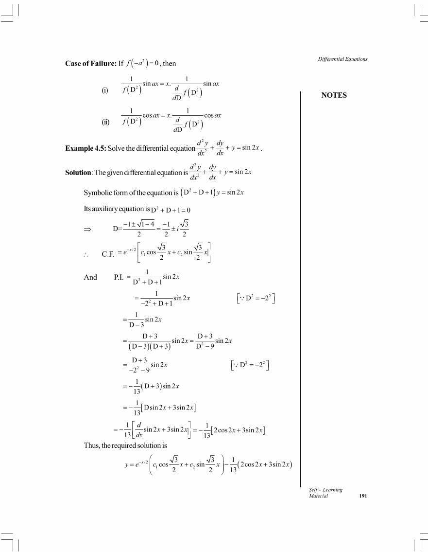
NOTES
Differential Equations
Self - LearningMaterial 191
Case of Failure: If 2 0f a , then
(i) 2
2
1 1sin . sin
D DD
ax x axdf f
d
(ii) 2
2
1 1cos . cos
D DD
ax x axdf f
d
Example 4.5: Solve the differential equation2
2sin 2
d y dyy x
dxdx .
Solution: The given differential equation is2
2sin 2
d y dyy x
dxdx
Symbolic form of the equation is 2D D 1 sin 2y x
Its auxiliary equation is 2D D 1 0
1 1 4 1 3
D=2 2 2
i
C.F. / 2
1 2
3 3cos sin
2 2xe c x c x
And P.I. 2
1sin 2
D D 1x
2
1sin 2
2 D 1x
2 2D 2
1
sin 2D 3
x
2
D 3 D 3sin 2 sin 2
D 3 D 3 D 9x x
2
D 3sin 2
2 9x
2 2D 2
1D 3 sin 2
13x
1Dsin 2 3sin 2
13x x
1
sin 2 3sin 213
dx x
dx
12cos2 3sin 2
13x x
Thus, the required solution is
/ 21 2
3 3 1cos sin 2cos 2 3sin 2
2 2 13xy e c x c x x x
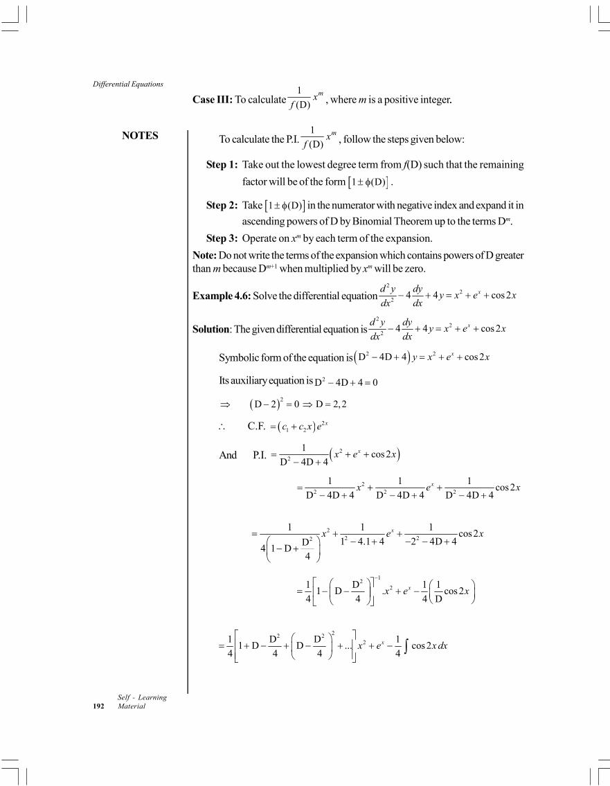
Differential Equations
NOTES
Self - Learning192 Material
Case III: To calculate1
(D)mx
f , where m is a positive integer..
To calculate the P.I.1
(D)mx
f , follow the steps given below:
Step 1: Take out the lowest degree term from f(D) such that the remaining
factor will be of the form 1 (D) .
Step 2: Take 1 (D) in the numerator with negative index and expand it in
ascending powers of D by Binomial Theorem up to the terms Dm.
Step 3: Operate on xm by each term of the expansion.
Note: Do not write the terms of the expansion which contains powers of D greaterthan m because Dm+1 when multiplied by xm will be zero.
Example 4.6: Solve the differential equation2
22
4 4 cos2xd y dyy x e x
dx dx
Solution: The given differential equation is2
22
4 4 cos2xd y dyy x e x
dx dx
Symbolic form of the equation is 2 2D 4D 4 cos2xy x e x
Its auxiliary equation is 2D 4D 4 0
2D 2 0 D 2,2
C.F. 21 2
xc c x e
And P.I. 22
1cos2
D 4D 4xx e x
22 2 2
1 1 1cos2
D 4D 4 D 4D 4 D 4D 4xx e x
22 22
1 1 1cos2
1 4.1 4 2 4D 4D4 1 D
4
xx e x
12
21 D 1 11 D . cos 2
4 4 4 Dxx e x
22 221 D D 1
1 D D ... cos24 4 4 4
xx e x dx
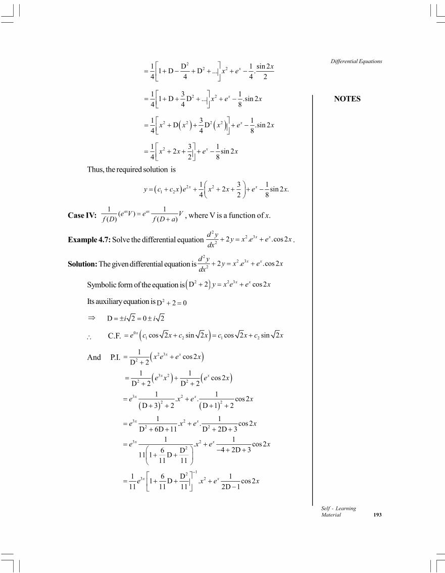
NOTES
Differential Equations
Self - LearningMaterial 193
2
2 21 D 1 sin 21 D D ... .
4 4 4 2x x
x e
2 21 3 1
1 D D ... .sin 24 4 8
xx e x
2 2 2 21 3 1D D .sin 2
4 4 8xx x x e x
21 3 1
2 sin 24 2 8
xx x e x
Thus, the required solution is
2 21 2
1 3 12 sin 2 .
4 2 8x xy c c x e x x e x
Case IV: 1 1
( )( ) ( )
ax axe V e Vf D f D a
, where V is a function of x.
Example 4.7: Solve the differential equation 2
2 32
2 . .cos 2x xd yy x e e x
dx .
Solution: The given differential equation is2
2 32
2 . .cos 2x xd yy x e e x
dx
Symbolic form of the equation is 2 2 3D 2 cos2x xy x e e x
Its auxiliary equation is 2D 2 0
D 2 0 2i i
C.F. 01 2 1 2cos 2 sin 2 cos 2 sin 2xe c x c x c x c x
And P.I. 2 32
1cos2
D 2x xx e e x
3 22 2
1 1cos 2
D 2 D 2x xe x e x
3 2
2 2
1 1. . cos 2
D 3 2 D 1 2x xe x e x
3 22 2
1 1. . cos 2
D 6D 11 D 2D 3x xe x e x
3 2
2
1 1. cos 2
4 2D 36 D11 1 D
11 11
x xe x e x
123 21 6 D 1
1 D . cos211 11 11 2D 1
x xe x e x
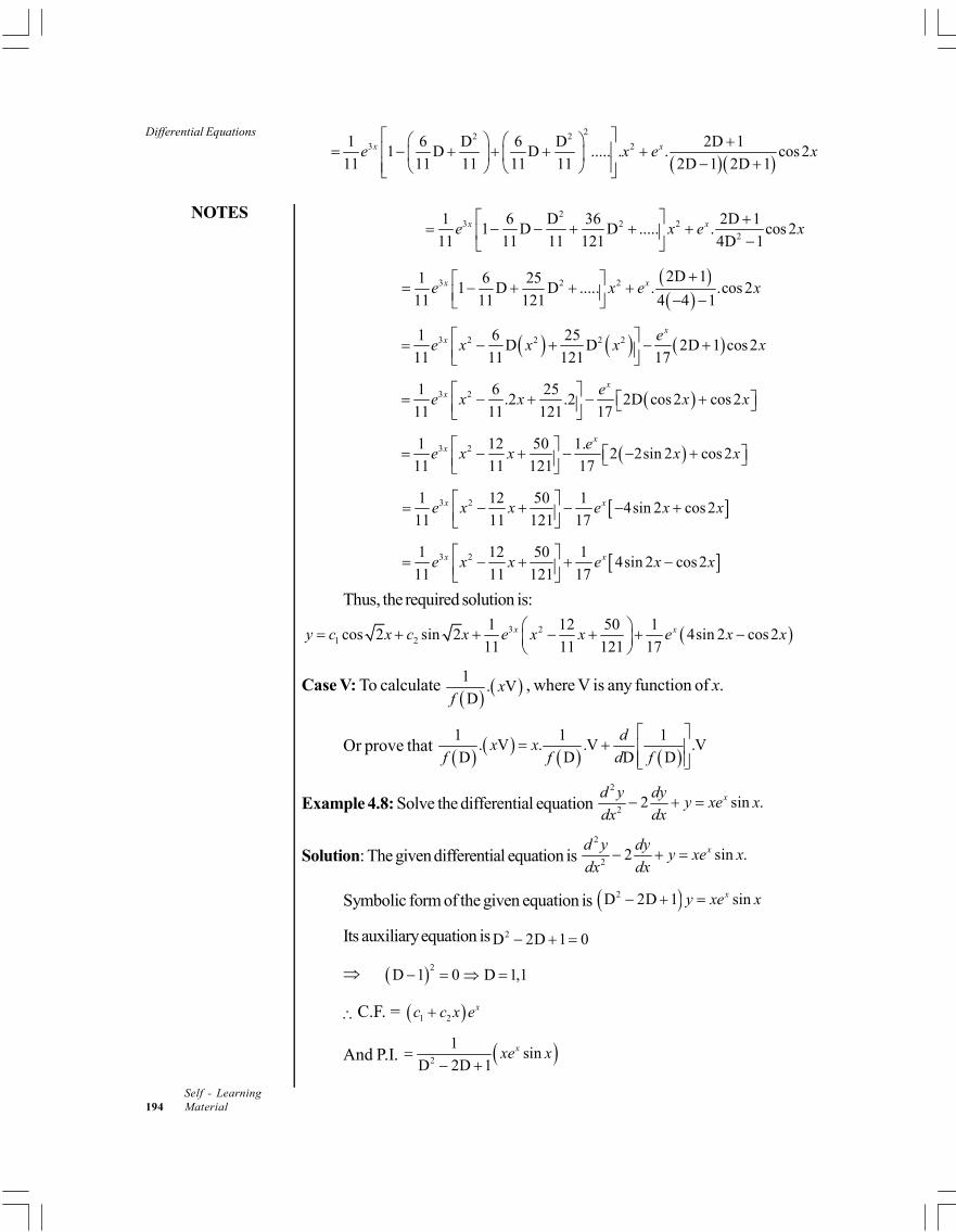
Differential Equations
NOTES
Self - Learning194 Material
22 23 21 6 D 6 D 2D 1
1 D D ..... . . cos211 11 11 11 11 2D 1 2D 1
x xe x e x
2
3 2 22
1 6 D 36 2D 11 D D ..... . cos 2
11 11 11 121 4D 1x xe x e x
3 2 2 2D 11 6 251 D D ..... . .cos 2
11 11 121 4 4 1x xe x e x
3 2 2 2 21 6 25D D 2D 1 cos2
11 11 121 17
xx e
e x x x x
3 21 6 25.2 .2 2D cos2 cos2
11 11 121 17
xx e
e x x x x
3 21 12 50 1.2 2sin 2 cos2
11 11 121 17
xx e
e x x x x
3 21 12 50 14sin 2 cos2
11 11 121 17x xe x x e x x
3 21 12 50 14sin 2 cos2
11 11 121 17x xe x x e x x
Thus, the required solution is:
3 21 2
1 12 50 1cos 2 sin 2 4sin 2 cos2
11 11 121 17x xy c x c x e x x e x x
Case V: To calculate 1
. VD
xf
, where V is any function of x.
Or prove that 1 1 1
. V . .V .VD D D D
dx x
f f d f
Example 4.8: Solve the differential equation 2
22 sin .xd y dy
y xe xdx dx
Solution: The given differential equation is 2
22 sin .xd y dy
y xe xdx dx
Symbolic form of the given equation is 2D 2D 1 sinxy xe x
Its auxiliary equation is 2D 2D 1 0
2D 1 0 D 1,1
C.F. = 1 2xc c x e
And P.I. 2
1sin
D 2D 1xxe x
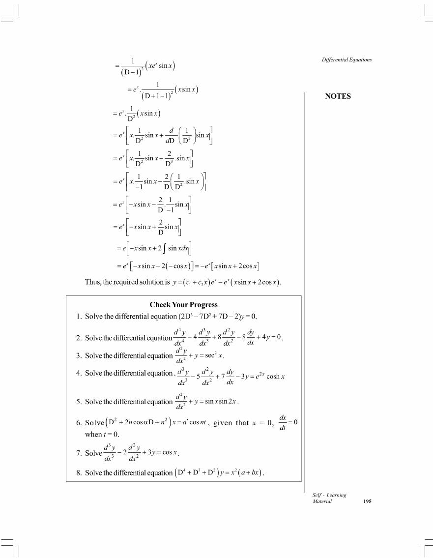
NOTES
Differential Equations
Self - LearningMaterial 195
2
1sin
D 1xxe x
2
1. sin
D 1 1xe x x
2
1. sinD
xe x x
2 2
1 1. sin sinD D D
x de x x x
d
2 3
1 2. sin .sinD D
xe x x x
2
1 2 1. sin .sin
1 D Dxe x x x
2 1
sin . sinD 1
xe x x x
2
sin sinD
xe x x x
sin 2 sine x x xdx sin 2 cos sin 2cosx xe x x x e x x x
Thus, the required solution is 1 2 sin 2cos .x xy c c x e e x x x
Check Your Progress
1. Solve the differential equation (2D3 – 7D2 + 7D – 2)y = 0.
2. Solve the differential equation4 3 2
4 3 24 8 8 4 0
d y d y d y dyy
dxdx dx dx .
3. Solve the differential equation 2
22
secd y
y xdx
.
4. Solve the differential equation .3 2
23 2
5 7 3 coshxd y d y dyy e x
dxdx dx
5. Solve the differential equation 2
2sin sin 2
d yy x x
dx .
6. Solve 2 2D 2 cos D cosn n x a nt , given that x = 0, 0dx
dt
when t = 0.
7. Solve3 2
3 22 3 cos
d y d yy x
dx dx .
8. Solve the differential equation 4 3 2 2D D D y x a bx .
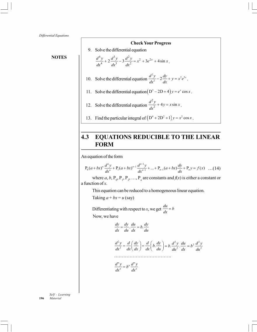
Differential Equations
NOTES
Self - Learning196 Material
Check Your Progress
9. Solve the differential equation4 3 2
2 24 3 2
2 3 3 4sinxd y d y d yx e x
dx dx dx .
10. Solve the differential equation 2
2 32
2 xd y dyy x e
dx dx .
11. Solve the differential equation 3D 2D 4 cosxy e x .
12. Solve the differential equation 2
24 sin
d yy x x
dx .
13. Find the particular integral of 4 2 2D 2D 1 cosy x x .
4.3 EQUATIONS REDUCIBLE TO THE LINEARFORM
An equation of the form
1
10 1 11
P ( ) P ( ) ... P ( ) P ( )n n
n nn nn n
d y d y dya bx a bx a bx y f x
dx dx dx
…(14)
where a, b, P0, P
1, P
2, …, P
n are constants and f(x) is either a constant or
a function of x.
This equation can be reduced to a homogeneous linear equation.
Taking a + bx = u (say)
Differentiating with respect to x, we get du
bdx
Now, we have
.dy dy du
dx du dx .
dyb
du
2
2
d y d dy
dx dx dx
.dyd
bdx du
2
2. .d y du
bdxdu
2
2
2
d yb
du
……………………………….n n
nn n
d y d yb
dx dx
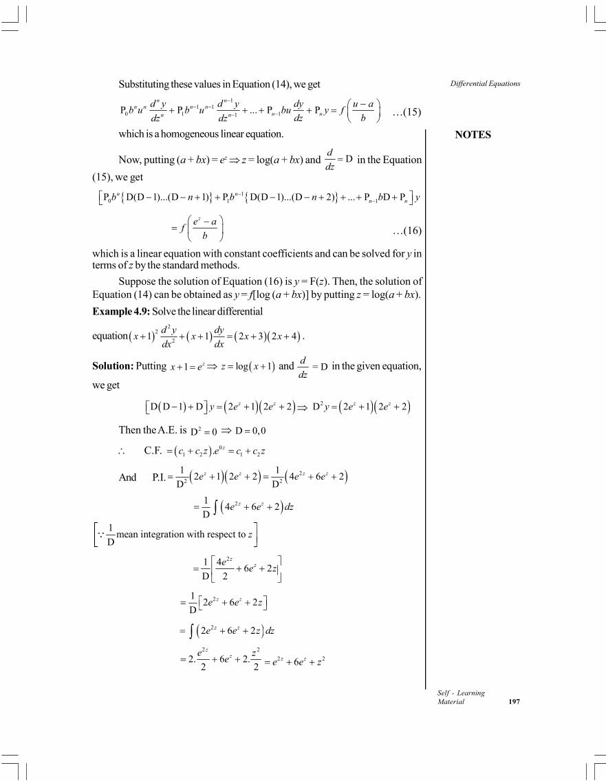
NOTES
Differential Equations
Self - LearningMaterial 197
Substituting these values in Equation (14), we get1
1 10 1 11
P P ... P Pn n
n n n nn nn n
d y d y dy u ab u b u bu y f
dz bdz dz
…(15)
which is a homogeneous linear equation.
Now, putting (a + bx) = ez z = log(a + bx) and Dd
dz in the Equation
(15), we get
10 1 1P D(D 1)...(D 1) P D(D 1)...(D 2) ... P D Pn n
n nb n b n b y
ze af
b
…(16)
which is a linear equation with constant coefficients and can be solved for y interms of z by the standard methods.
Suppose the solution of Equation (16) is y = F(z). Then, the solution ofEquation (14) can be obtained as y = f[log (a + bx)] by putting z = log(a + bx).
Example 4.9: Solve the linear differential
equation 2
2
21 1 2 3 2 4
d y dyx x x x
dx dx .
Solution: Putting 1 zx e log 1z x and = Dd
dz in the given equation,
we get
D D 1 D 2 1 2 2z zy e e 2D 2 1 2 2z zy e e
Then the A.E. is 2D 0 D 0,0
C.F. 01 2 1 2. zc c z e c c z
And P.I. 22 2
1 12 1 2 2 4 6 2
D Dz z z ze e e e
214 6 2
Dz ze e dz
1mean integration with respect to
Dz
21 4
6 2D 2
zze
e z
212 6 2
Dz ze e z
22 6 2z ze e z dz
2 2
2. 6 2.2 2
zze z
e 2 26z ze e z
Differential Equations
NOTES
Self - Learning198 Material
Thus, the solution of the given equation is y = C.F. + P.I.
2 21 2 6z zy c c z e e z
22
1 2 log 1 1 6 1 log 1y c c x x x x
1 log 1ze x z x
221 2 .log 1 8 log 1y c c x x x x
[Constant term 7 can be considered to be included in 1c ]
Check Your Progress
14. Which equation form can be reduced to the homogeneous linear equation?
4.4 EXACT DIFFERENTIAL EQUATIONS
A differential equation which can be obtained from its solution ,f x y c directly
by differentiation without any further multiplication, elimination is called an exactdifferential equation.
We can define the exact differential equations in another way also.
The differential equation M N 0dx dy , where M and N are the functions
of x and y is called exact if there exist a function F ,x y such that M N Fdx dy d
(i.e., M N dx dy is an exact differential of a function of x and y) and F(x, y) = cis its solution.
The following differential equations are exact:
(i) 0xdy ydx because xdy + ydx = d(xy) and xy = c
(ii) 20
xdy ydx
x
because 2
xdy ydx yd
x x
and y
cx
(iii) sin cos cos sin 0x ydy x ydx because sin x cosydy+cos x sin ydx=d
(sin x sin y) and sin sinx y = c
Theorem 4.3: The necessary and sufficient condition for the ordinary differential
equation M N 0dx dy to be exact is M N
y x
.
Proof: Necessary Condition
Let the given equation M N 0dx dy be exact.
Then by definition there exists a function F ,x y such that
M N Fdx dy d …(17)
NOTES
Differential Equations
Self - LearningMaterial 199
Also, from differential calculus, we know that
F FFd dx dy
x y
…(18)
Comparing Equations (17) and (18), we get
FM
x
and
FN
y
2M F F
y y x y x
and
2N F F
x x y x y
As,2 2F F
y x x y
, thusM N
y x
which is the required condition for the equation M N 0dx dy to be exact.
Sufficient Condition
Let M N
y x
. Then, we have to show that M N 0dx dy is an exact differential
equation.
Let M ,dx x y …(19)
where M ,x y is integrated with respect to x taking y as a constant such that
Mdxx x
Mx
…(20)
2M
y y x y x
2N
x y x
M N
y x
Also,2 2
y x x y
2N
x x y x y
Integrating with respect to x, taking y as a constant, we get
N g yy
…(21)
where g y is a function of y.
Using Equations (20) and (21), we get
M Ndx dy dx dy g y dyx y
d d g y dy
d g y dy
which is an exact differential.
Differential Equations
NOTES
Self - Learning200 Material
Solving an Exact Differential Equation
If M N 0dx dy is an exact differential equation, then from the above section,we have
0d g y dy
Integrating, we get
g y dy c , where c is an arbitrary constant …(22)
From Equation (19), we have
constant
M
y
dx Putting the value of in Equation (21), we get
constant
M
y
dx g y dy c
constant
M (Terms of N not conatining )
y
dx x dy c which is the required solution.
Example 4.10: Solve the differential
equation 4 2 4 2 32 2 4 sin 0x xy y dx x y xy y dy .
Solution: The given equation is
4 2 4 2 32 2 4 sin 0x xy y dx x y xy y dy …(i)
We know that M N 0dx dy …(ii)
Comparing Equations (i) and (ii), we get 4 2 4M 2x xy y and2 3N 2 4 sinx y xy y
Now,3M
4 4xy yy
and 3N4 4xy y
x
Since M N
y x
, thus the Equation (i) is exact and its solution is given by
constant
M Terms of N not containing
y
dx x dy c 4 2 4
constant
2 sin
y
x xy y dx y dy c
5 22 42 . . cos
5 2
x xy y x y c
52 2 4 cos
5
xx y xy y c
which is the required solution.
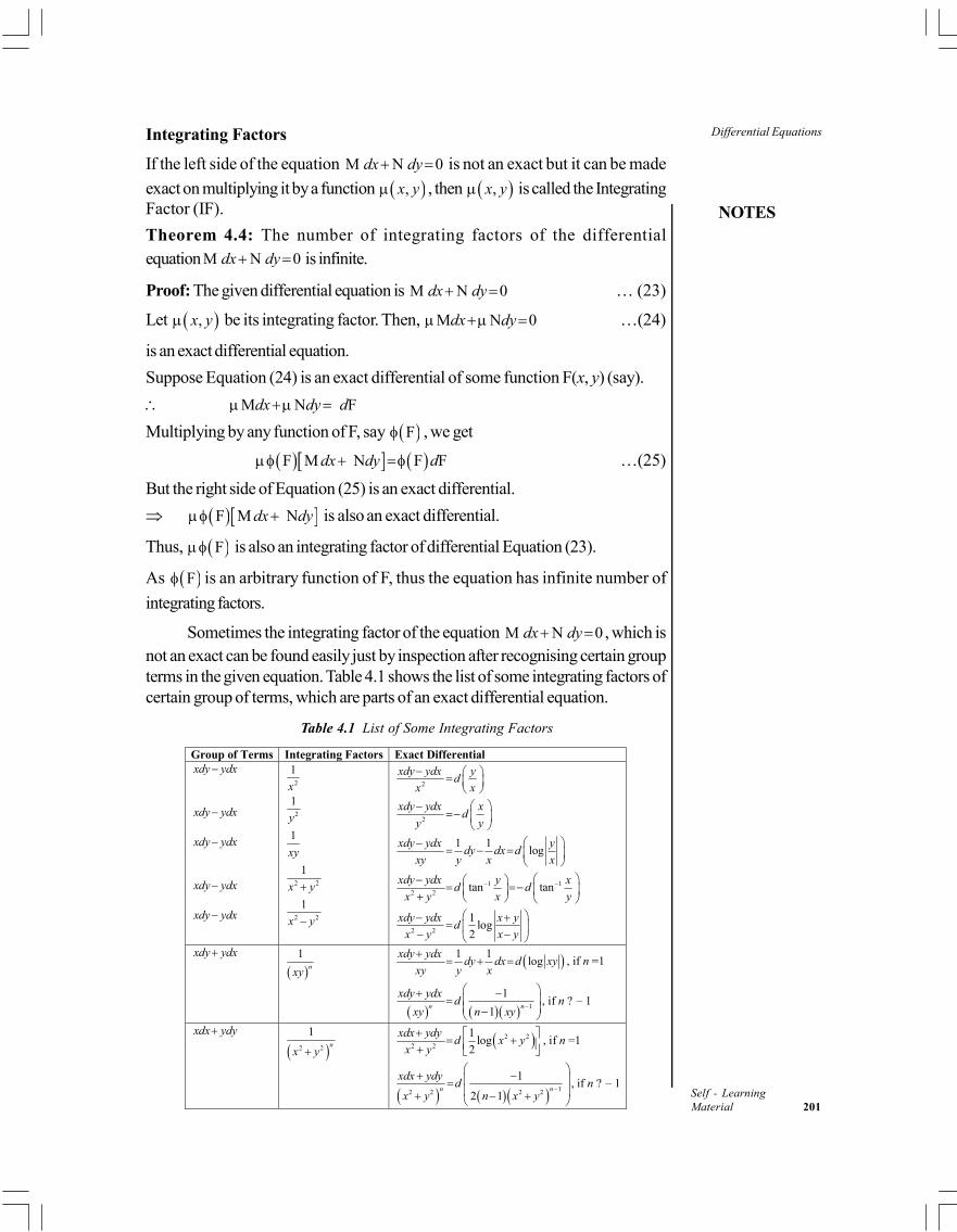
NOTES
Differential Equations
Self - LearningMaterial 201
Integrating Factors
If the left side of the equation M N 0dx dy is not an exact but it can be made
exact on multiplying it by a function ,x y , then ,x y is called the IntegratingFactor (IF).
Theorem 4.4: The number of integrating factors of the differentialequation M N 0dx dy is infinite.
Proof: The given differential equation is M N 0dx dy … (23)
Let ,x y be its integrating factor. Then, M N 0dx dy …(24)
is an exact differential equation.
Suppose Equation (24) is an exact differential of some function F(x, y) (say).
M N Fdx dy d
Multiplying by any function of F, say F , we get
F M N F Fdx dy d …(25)
But the right side of Equation (25) is an exact differential.
F M Ndx dy is also an exact differential.
Thus, F is also an integrating factor of differential Equation (23).
As F is an arbitrary function of F, thus the equation has infinite number of
integrating factors.
Sometimes the integrating factor of the equation M N 0dx dy , which isnot an exact can be found easily just by inspection after recognising certain groupterms in the given equation. Table 4.1 shows the list of some integrating factors ofcertain group of terms, which are parts of an exact differential equation.
Table 4.1 List of Some Integrating Factors
Group of Terms Integrating Factors Exact Differential xdy ydx xdy ydx xdy ydx xdy ydx xdy ydx
2
1
x
2
1
y
1
xy
2 2
1
x y
2 2
1
x y
2
xdy ydx yd
x x
2
xdy ydx xd
y y
1 1log
xdy ydx ydy dx d
xy y x x
1 12 2
tan tanxdy ydx y x
d dx y x y
2 2
1log
2
xdy ydx x yd
x y x y
xdy ydx
1
nxy
1 1log
xdy ydxdy dx d xy
xy y x
, if n =1
1
1
1n n
xdy ydxd
xy n xy
, if n ? – 1
xdx ydy
2 2
1n
x y 2 2
2 2
1log
2
xdx ydyd x y
x y
, if n =1
12 2 2 2
1
2 1n n
xdx ydyd
x y n x y
, if n ? – 1
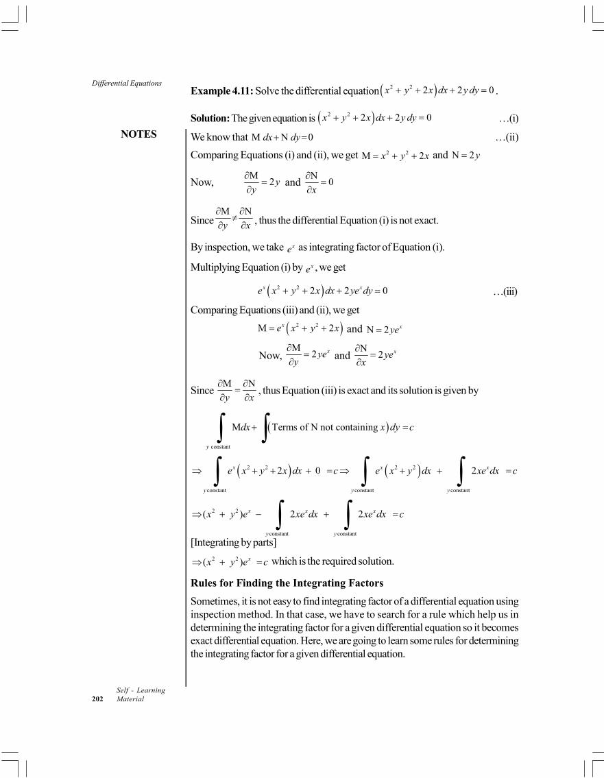
Differential Equations
NOTES
Self - Learning202 Material
Example 4.11: Solve the differential equation 2 2 2 2 0x y x dx y dy .
Solution: The given equation is 2 2 2 2 0x y x dx y dy …(i)
We know that M N 0dx dy …(ii)
Comparing Equations (i) and (ii), we get 2 2M 2x y x and N 2y
Now,M
2yy
and
N0
x
SinceM N
y x
, thus the differential Equation (i) is not exact.
By inspection, we take xe as integrating factor of Equation (i).
Multiplying Equation (i) by xe , we get
2 2 2 2 0x xe x y x dx ye dy …(iii)
Comparing Equations (iii) and (ii), we get
2 2M 2xe x y x and N 2 xye
Now, M
2 xyey
and
N2 xye
x
Since M N
y x
, thus Equation (iii) is exact and its solution is given by
constant
M Terms of N not containing
y
dx x dy c 2 2
constant
2 0x
y
e x y x dx c 2 2
constant constant
2x x
y y
e x y dx xe dx c 2 2
constant constant
( ) 2 2x x x
y y
x y e xe dx xe dx c [Integrating by parts]
2 2( ) xx y e c which is the required solution.
Rules for Finding the Integrating Factors
Sometimes, it is not easy to find integrating factor of a differential equation usinginspection method. In that case, we have to search for a rule which help us indetermining the integrating factor for a given differential equation so it becomesexact differential equation. Here, we are going to learn some rules for determiningthe integrating factor for a given differential equation.
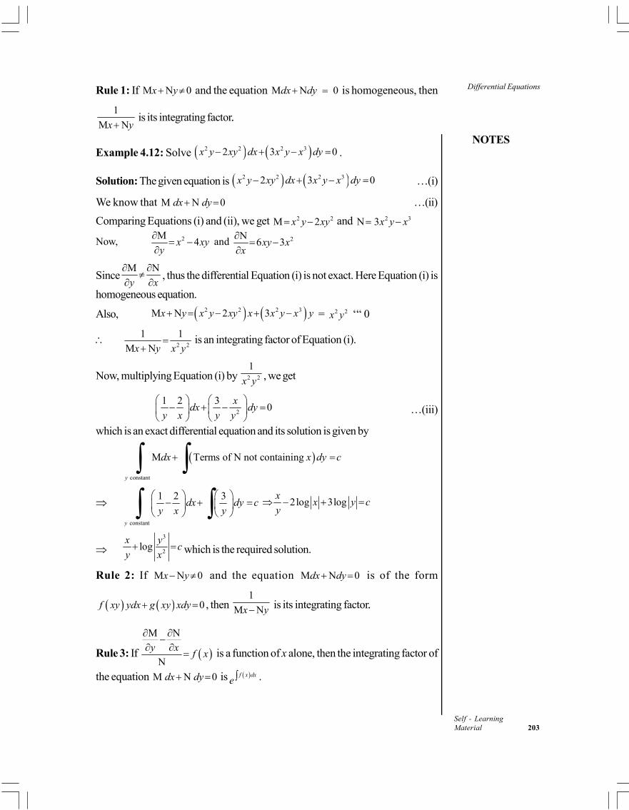
NOTES
Differential Equations
Self - LearningMaterial 203
Rule 1: If M N 0x y and the equation M N 0dx dy is homogeneous, then
1
M Nx y is its integrating factor..
Example 4.12: Solve 2 2 2 32 3 0x y xy dx x y x dy .
Solution: The given equation is 2 2 2 32 3 0x y xy dx x y x dy …(i)
We know that M N 0dx dy …(ii)
Comparing Equations (i) and (ii), we get 2 2M 2x y xy and 2 3N 3x y x
Now, 2M4x xy
y
and 2N
6 3xy xx
SinceM N
y x
, thus the differential Equation (i) is not exact. Here Equation (i) is
homogeneous equation.
Also, 2 2 2 3M N 2 3x y x y xy x x y x y = 2 2x y ‘“ 0
2 2
1 1
M Nx y x y
is an integrating factor of Equation (i).
Now, multiplying Equation (i) by 2 2
1
x y , we get
2
1 2 30
xdx dy
y x y y
…(iii)
which is an exact differential equation and its solution is given by
constant
M Terms of N not containing
y
dx x dy c
constant
1 2 3
y
dx dy cy x y
2log 3logx
x y cy
3
2log
x yc
y x which is the required solution.
Rule 2: If M N 0x y and the equation M N 0dx dy is of the form
0f xy ydx g xy xdy , then 1
M Nx y is its integrating factor..
Rule 3: If
M N
N
y xf x
is a function of x alone, then the integrating factor of
the equation M N 0dx dy is f x dxe .
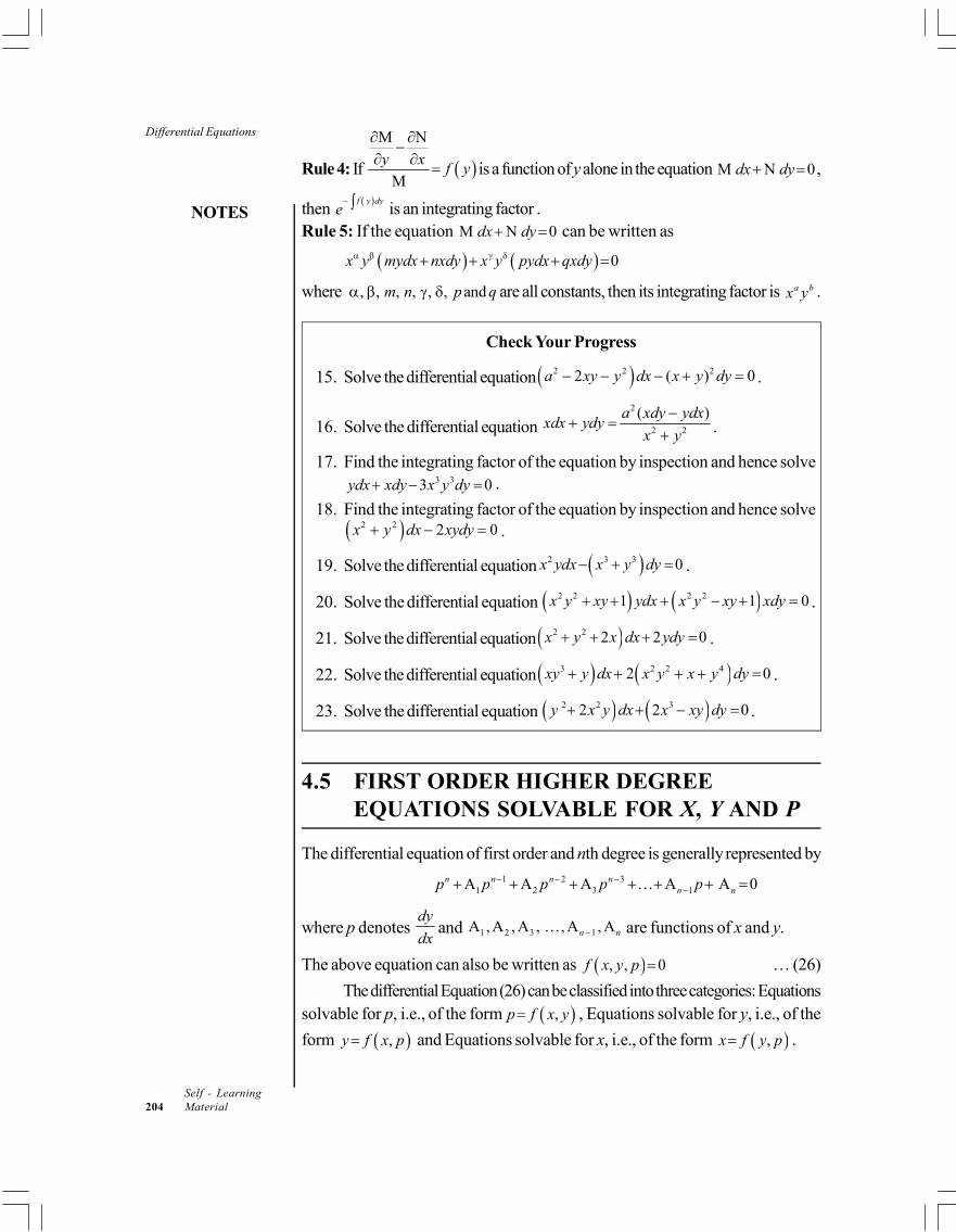
Differential Equations
NOTES
Self - Learning204 Material
Rule 4: If
M N
M
y xf y
is a function of y alone in the equation M N 0dx dy ,
then f y dy
e is an integrating factor .
Rule 5: If the equation M N 0dx dy can be written as
0x y mydx nxdy x y pydx qxdy
where , , , , , , andm n p q are all constants, then its integrating factor is a bx y .
Check Your Progress
15. Solve the differential equation 2 2 22 ( ) 0a xy y dx x y dy .
16. Solve the differential equation 2
2 2
( )a xdy ydxxdx ydy
x y
.
17. Find the integrating factor of the equation by inspection and hence solve3 33 0ydx xdy x y dy .
18. Find the integrating factor of the equation by inspection and hence solve 2 2 2 0x y dx xydy .
19. Solve the differential equation 2 3 3 0x ydx x y dy .
20. Solve the differential equation 2 2 2 21 1 0x y xy ydx x y xy xdy .
21. Solve the differential equation 2 2 2 2 0x y x dx ydy .
22. Solve the differential equation 3 2 2 42 0xy y dx x y x y dy .
23. Solve the differential equation 2 2 32 2 0y x y dx x xy dy .
4.5 FIRST ORDER HIGHER DEGREEEQUATIONS SOLVABLE FOR X, Y AND P
The differential equation of first order and nth degree is generally represented by1 2 3
1 2 3 1A A A A A 0n n n nn np p p p p
where p denotes dy
dxand 1 2 3 1A , A , A , , A , An n are functions of x and y.
The above equation can also be written as , , 0f x y p … (26)
The differential Equation (26) can be classified into three categories: Equationssolvable for p, i.e., of the form ,p f x y , Equations solvable for y, i.e., of the
form ,y f x p and Equations solvable for x, i.e., of the form ,x f y p .
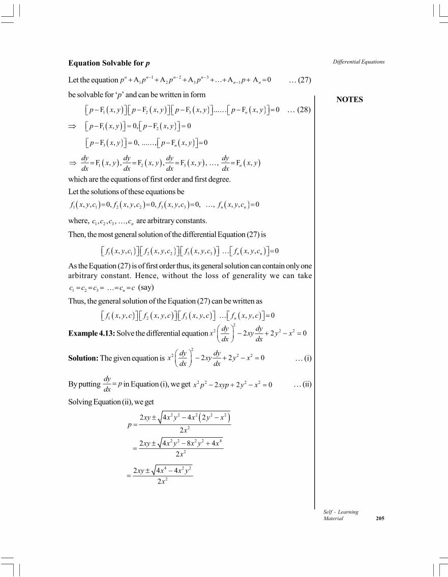
NOTES
Differential Equations
Self - LearningMaterial 205
Equation Solvable for p
Let the equation 1 2 31 2 3 1A A A A A 0n n n n
n np p p p p … (27)
be solvable for ‘p’ and can be written in form
1 2 3F , F , F , ... F , 0np x y p x y p x y p x y … (28)
1 2F , 0, F , 0,p x y p x y
3F , 0,p x y ... , F , 0np x y
1 2 3F , , F , , F , , , F ,n
dy dy dy dyx y x y x y x y
dx dx dx dx
which are the equations of first order and first degree.
Let the solutions of these equations be
1 1 2 2 3 3, , 0, , , 0, , , 0,f x y c f x y c f x y c , , , 0n nf x y c
where, 1 2 3, , , , nc c c c are arbitrary constants.
Then, the most general solution of the differential Equation (27) is
1 1 2 2 3 3, , , , , , , , 0n nf x y c f x y c f x y c f x y c
As the Equation (27) is of first order thus, its general solution can contain only onearbitrary constant. Hence, without the loss of generality we can take
1 2 3 nc c c c c (say)
Thus, the general solution of the Equation (27) can be written as
1 2 3, , , , , , , , 0nf x y c f x y c f x y c f x y c
Example 4.13: Solve the differential equation2
2 2 22 2 0dy dy
x xy y xdx dx
Solution: The given equation is 2
2 2 22 2 0dy dy
x xy y xdx dx
… (i)
By putting dy
pdx
in Equation (i), we get 2 2 2 22 2 0x p xyp y x … (ii)
Solving Equation (ii), we get
2 2 2 2 2
2
2 4 4 2
2
xy x y x y xp
x
2 2 2 2 4
2
2 4 8 4
2
xy x y x y x
x
4 2 2
2
2 4 4
2
xy x x y
x
Differential Equations
NOTES
Self - Learning206 Material
2 2 2
2
2 4
2
xy x x y
x
2 2 2 2
2
2 2
2
xy x x y y x y
x x
2 2y x ydy
dx x
…(iii)
which is a homogeneous equation in x and y.Let y vxDifferentiating both sides with respect to x, we get
dy dvv x
dx dx
By putting the values of y and dy
dxin Equation (iii), we get
2 2 2dv vx x v x
v xdx x
21dv
v x v vdx
21dv
x vdx
Separating the variables, we get
21
dv dx
xv
Integrating both sides, we get
21
dv dxc
xv
1sin log logv x c 1sin logv xc 1sin log ,y
cxx
which is the required solution.
Equation Solvable for y
A differential Equation is said to be solvable y, if it can be expressed as
,y f x p … (29)
Differentiating both sides with respect to x, we get
F , ,dy dp
p x pdx dx
… (30)
The differential Equation (ii) is in two variables p and x.
Let the solution of the Equation (ii) be
, , 0x p c … (31)
So, by eliminating p from Equation (29) and Equation (31), we get thesolution of differential Equation (29). If it is not easier to eliminate p, then putEquations (29) and (31) in the form
1 2, , ,x p c y p c
NOTES
Differential Equations
Self - LearningMaterial 207
In this case these two equations together constitute the solution of Equation (29).
Note: When the Equation (30) can be written as 1 2( , ). , ,dp
f x p f x pdx
= 0, neglect
the factor which does not contain dp
dx, i.e., 1( , )f x p since if 1( , )f x p = 0, then
elimination of p from this equation and Equation (29) does not give a generalsolution.
Example 4.14: Solve the differential equation 3 log .y x p
Solution: The given equation is 3 logy x p … (i)
Differentiating both sides with respect to x, we get
13
dy dp
dx p dx
13
dpp
p dx
dyp
dx
3
dpdx
p p
1 1 1
3 3dx dp
p p
(By Partial Fraction)
Integrating both sides, we get
1
1log 3 log log
3x p p c
2
33 log log
px c
p
2
33 log .
px c
p
Taking exponent of both sides, we get
32
3.x p
e cp
33 xpce
p
33
1 xcep
3
3
1 xp
ce
Substituting this value of p in Equation (i), we get 3
33 log
1 xy x
ce
which is the required solution.
Equation Solvable for x
A differential equation is said to be solvable for x, if x can be expressed as
,x f y p … (32)
Differentiating both sides with respect to y, we get 1
F , ,dx dp
y pdy p dy
… (33)
The differential Equation (33) is in two variables y and p.
Let the solution of the Equation (33) be , , 0y p c … (34)
Then, by eliminating p from Equations (32) and (34), we get the solution ofdifferential Equation (32). If it is not easier to eliminate p, then express Equation(32) and (34) in the form
1 2, , ,x p c y p c
Differential Equations
NOTES
Self - Learning208 Material
In such case, the above two equations taken together constitute the solution ofEquation (32).
Note: When the Equation (33) is written as 1 2( , ). , ,dp
f y p f y pdy
= 0, then neglect
the factor which does not contain dp
dy , i.e., 1( , )f y p , since if 1( , )f y p = 0, then
eliminating p from this equation Equation (33) doe not give a general solution.
Example 4.15: Solve the differential equation 2x y p
Solution: The given equation is 2x y p … (i)
Differentiating both sides with respect to y, we get
1 2dx dp
pdy dy
11 2
dpp
p dy 21 2
dpp p
dy
22
1
pdy dp
p
Integrating both sides, we get
22
1
pdy dp c
p
1
2 11
y p dp cp
2
2 log 12
py c p p
2 2 2log 1y c p p p
Substituting the value of y in Equation (i), we get
2 2 log 1x c p p which is the required solution.
Check Your Progress
24. Solve the differential equation 2 2 2 2 0xyp x xy y p x xy .
25. Solve the differential equation4 2
2 2
2 2
21 0
y y yy p p
xx x
.
26. Solve the differential equation y = p tan p + log cos p.
27. Solve the differential equation y – 2px = f(xp2).
28. Solve the differential equation 2tan
1
pp x
p
.
NOTES
Differential Equations
Self - LearningMaterial 209
4.6 CLAIRAUT’S EQUATION
The differential equation of the form y px f p is termed as Clairaut’ss
Equation.
Solution of Clairaut’s Equation
The given equation is y px f p … (35)
Differentiating both sides with respect to x, we get
dy dp dpp x f p
dx dx dx
dp dpp p x f p
dx dx 0
dpx f p
dx
Neglecting x f p , we get 0dp
dx
Integrating both sides, we get p = cSubstituting the value of p in Equation (35), we get
y cx f c , which is the required solution.
Here, we neglect x f p because if we eliminate p between the given
Equation (35) and the factor x f p =0, we get another solution termed as
singular solution.
Note: When equation is in the Clairaut’s form, then the solution can be writtendown just by changing p to c in the given equation.
Example 4.16: Solve the differential equation sin cos cos sinpx y px y p andobtain the singular solution.
Solution: The given differential equation is sin cos cos sinpx y px y p
sin cos cos sinpx y px y p
sin px y p
1sinpx y p 1siny px p … (i)
which is a Clairaut’s form.
Thus the solution is 1siny cx c [Replacing p by c] … (ii)
Differentiating Equation (ii) partially with respect to c, we have
2
10
1x
c
2 1xc
x
Differential Equations
NOTES
Self - Learning210 Material
Substituting the value of c in Equation (ii), we get
22 1 1
1 sinx
y xx
, which is the required singular solution.
4.7 SINGULAR SOLUTIONS
A singular solution is a solution of differential equation which cannot be obtainedfrom its general solution by assigning any particular values to the arbitrary constants.
Discriminant
The discriminant of a polynomial is an expression which gives information aboutthe nature of the polynomial’s roots. We know that the discriminant of the quadratic
equation 2 0ax bx c is 2 4b ac . Here, if 2 4b ac > 0, the equation has two
real roots, if 2 4b ac = 0, the equation has equal roots which are real, and
if 2 4b ac < 0, the equation has two imaginary roots. But if equation has higher
degree than two, then the condition that the equation 0f x has two equal roots
is obtained by eliminating x between 0f x and 0f x .
p-Discriminant and c-Discriminant dy
pdx
Let , , 0f x y p … (36)
be the differential equation having
, , 0x y c … (37)
as the solution, where, c is an arbitrary constant.
Differentiating both sides of Equation (37) partially with respect to c, we get
, , 0x y cc
… (38)
Differentiating both sides of Equation (36) partially with respect to p, we get
, , 0f x y pp
… (39)
By eliminating c between the Equations (37) and (38), we get c-discriminant.Thus, c-discriminant represents the locus of each point which has equal values of
c in , , 0x y c .
By eliminating p between the Equations (36) and (39), we get p-discriminant.Thus, p-discriminant represents the locus of each point which has equal values ofp in
, , 0f x y p .
Note: (i) The envelope which is present in both c-discriminant and p-discriminantis known as the singular solution.
NOTES
Differential Equations
Self - LearningMaterial 211
(ii) If the singular solution of a differential equation , , 0f x y p whose
primitive is , , 0x y c is given by F , 0x y , then F ,x y will be a
factor of both the discriminates. (iii) In the Clairaut’s form of the differential equation both c-discriminant
and p-discriminant are same.
Method For Determining Singular Solution
Use the following steps to find the singular solutions of a differential equation
, , 0f x y p … (40)
Step 1: Find its complete solution , , 0x y c … (41)
where, c is an arbitrary constant.
Step 2: Find p-discriminant of Equation (40) and c-discriminant of Equation (41).Both contain the singular solution.
Now, when p-discriminant is equated to zero, it may include the followingas a factor:
Envelope, i.e., singular solution once (E) Cusp locus once (C) Tac locus, twice (T 2)
So p-discriminant 2ET C , which does not contain nodal locus and whenc-discriminant is equated to zero it may include the following as a factor:
Envelope, i.e, singular solution once (E) Cusp locus thrice (C3) Nodal locus twice (N 2)
So c-discriminant 2 3EN C
Example 4.17: Obtain the primitive and the singular solution of
2
2 4 0dy dy
x y xdx dx
Solution: The given differential equation is 2
2 4 0dy dy
x y xdx dx
… (i)
By putting dy
pdx
in Equation (i), we get
2 2 4 0xp yp x …(ii)
2
2
xp xy
p
Differentiating both sides, with respect to x, we get
2
2 2.
2 2
dy x dp p x dp
dx dx p p dx
Differential Equations
NOTES
Self - Learning212 Material
2
2 2. .
2 2
dp p dpx xp
dx p dxp
2
2 2
2 2
p x x dp
p p dx
2
22
44
2 2
p x dpp
p p dx
2 4 1 0x dp
pp dx
2 4 0p or 1 . 0x dp
p dx 2p or . 1
x dp
p dx
Now, for . 1x dp
p dx
dp dx
p x [Separating the variables]
Integrating both sides, we getlog log logp x c
where c is any arbitrary constant
log logp cx p cx … (iii)
Substituting the value of p from Equation (iii) in Equation (ii), we get
2 3 2 4 0c x ycx x 2 2 2 4 0c x yc … (iv)
which is the complete primitive of Equation (i),
From Equation (iv), we have p-discriminant (ET2C) is 2 24 16 0y x
2 24 0y x
Also from Equation (ii), c-discriminant (EN2C3) is 2 24 16 0y x
Since, 2 24y x is non-repeated common factor in p and c-discriminants and it
satisfies the differential Equation (ii).
Hence the singular solution of Equation (i) is
2 24 0y x 2y x
Check Your Progress
29. Reduce the differential equation 2px y x py p to Clairaut’s form
by substituting 2x u and 2y v . Also, find its complete primitive and its
singular solution.
30. Solve the differential equation 2y px p and obtain the singular solution.
31. Examine the equation 2 2 2 22 1y pxy p x m for singular solution.
NOTES
Differential Equations
Self - LearningMaterial 213
4.8 ORTHOGONAL TRAJECTORIES
A curve which cuts every member of a given family of curves according to adefinite law is called a trajectory of the given family.
Orthogonal Trajectory
A curve which cuts every member of a given family of curves at right angles iscalled an orthogonal trajectory of the given family.
Orthogonal trajectories of a given family of curves, themselves form a familyof curves.
We know that the angle between the two curves is equal to the angle betweenthe tangents at their common point of intersection. The slope of these tangents is
given by dy
dx.
When the curves intersects orthogonally,
Product of their slopes = – 1
Let the common point of intersection of two curves c1 and c
2 be P and the
angle between these curves at P is right angle, then
1 2 1 2
1c c c c
dy dy dy dx
dx dx dx dy
Oblique Trajectory
A curve which cuts every member of a given family of curves at certain angle otherthan right angle is called an oblique trajectory of the given family.
Differential Equation of Orthogonal Trajectories
Cartesian Coordinates
Step 1: Let the equation of the given family of curves be
f(x, y, c) = 0 … (42)where c is the parameter of the family.
Step 2: Differentiating Equation (42) with respect to x and eliminating c betweenEquation (42) and the resulting equation, we get the differential equation of thegiven family as
, , 0dy
F x ydx
… (43)
Step 3: Putting dy
dx=
dx
dy in Equation (43), we get
, , 0dx
F x ydy
… (44)
which is the differential equation of orthogonal trajectory.
Differential Equations
NOTES
Self - Learning214 Material
Step 4: Integrate Equation (44) to get the required equation of orthogonaltrajectories.
Example 4.18: Find the orthogonal trajectories of the family of co-axial circles x2
+ y2 + 2gx + c = 0, where g is a parameter and c is a constant.
Solution: The given equation is x2 + y2 + 2gx + c = 0 … (i)
Differentiating Equation (i) with respect to x, we get
2 2 2 0dy
x y gdx
0dy
x y gdx
… (ii)
Eliminating g between Equations (i) and (ii), we get the differential equation of the
given family of circles as 2 2 2 0dy
x y x x y cdx
2 2 2 0dy
y x xy cdx
… (iii)
By replacing dy
dx by
dx
dy
, we get
2 2 2 0dx
y x xy cdy
2 22
dxxy x c y
dy … (iv)
Let x2 = v. Then 2dx dv
xdy dy
The Equation (iv) becomes
2dvy v c y
dy
1dv cv y
dy y y
which is a linear differential equation in v.
1/
I.F.y dy
e = 1
1log
log logy y ye e e =
1
yThus, the required solution is
1 1cv y dy
y y y
1
vy
cy k
y , where k is an arbitrary constant
2v c y ky 2 2 0x y ky c
which is the orthogonal trajectories of the family of co-axial circles x2 + y2 + 2gx+ c = 0.
NOTES
Differential Equations
Self - LearningMaterial 215
Polar Co-Ordinates
Step 1: Let the equation of the given family of polar curves be
f(r, , c) = 0 … (45)
where c is the parameter of the family.
Step 2: Differentiating Equation (45) with respect to and eliminating c betweenEquation (45) and the resulting equation, we get the differential equation of thegiven family as
,θ, 0θ
drF r
d
… (46)
Step 3: From differential calculus, we know that d
rdr
is the tangent of the angle
between the tangent to a curve and the radius vector at any point (r, ). Since, thecurves intersects orthogonally,
1 2
1c c
d dr r
dr dr
, where c
1 and c
2 are two curves.
1
θ
d drr
dr r d
θ
dr
d= 2 d
rdr
Replace dr
d by 2 d
rdr
in (ii), we get
2, , 0d
F r rdr
… (47)
which is the differential equation of orthogonal trajectory.
Step 4: Integrate Equation (47) to get the required equation of the orthogonaltrajectories.
Example 4.19: Find the orthogonal trajectories of the curves sinn nr n a .
Solution: The given equation of the system of curve is sinn nr n a ... (i)
Taking log on both sides, we get
log logsin logn r n n a
Differentiating with respect to , we get
1 1. . cos 0
sin
drn n n
r d n
1
cot 0dr
nr d
tand
r ndr
... (ii)
Replacingdr
d by 2 d
rdr
in (ii) we get
1tan
drn
r d
tan
drn d
r
Differential Equations
NOTES
Self - Learning216 Material
Integrating, we get 1tandr
n d cr , where 1c is any arbitrary constant.
1log logsec logr n c
n
[Putting 1 logc c ]
1/log log sec log
nr n c
1/log log sec
nr c n
1/sec
nr c n secn nr c n cosn nr n c
which is required equation of the orthogonal trajectories.
Check Your Progress
32. Find the orthogonal trajectories of 2 2
2 21
x y
a b
, where l is a
parameter.
33. Find the orthogonal trajectories of the system of curves rn = an cos nq.
4.9 ANSWERS TO ‘CHECK YOUR PROGRESS’
1. y = c1ex + c
2e2x + c
3ex/2
2. 41 2 3cos sinxy e c c x x c c x x
3. 1 2cos sin sin log sec tan 1.y c x c x x x x
4. 3 3 21 2 3
1 1
8 8x x x xy c c x e c e xe x e .
5. 1 2
1cos sin sin cos3
4 16
xy c x c x x x
6. cos2
sin sin2 cos sin
n t ax e n t
n
2
'sin
2 cos
a nt
n
7.3
21 2 3
3 3cos sin
2 2
xxy c e e c x c x
15cos sin
26x x
8.2
1 2 3 4
3 3cos sin
2 2
x
y c c x e c x c x
4 5 3
23 312 20 3
x bx axa b bx
NOTES
Differential Equations
Self - LearningMaterial 217
9. 3 21 2 3 4
3
20x x xy c c x c e c e e
4
3 22 1 2 72sin cos
5 3 12 9 9
xx x x x
10. 3 21 2
12 4 3
8x xy c c x e e x x
11. 2 cos sinx xy ae b x c x e 3sin cos20
xxex x
12. 1 2
1 2cos2 sin 2 sin cos
3 9y c x c x x x x
13. 4 2 319 cos 4 sin
48x x x x x
14. An equation of the form,
11
0 1 11P ( ) P ( ) ... P ( ) P ( )
n nn n
n nn n
d y d y dya bx a bx a bx y f x
dx dx dx
where a, b, P0, P
1, P
2, …, P
n are constants and f(x) is either a constant or
a function of x.
This equation can be reduced to a homogeneous linear equation.
15.3
2 2 2
3
ya x x y xy c
16.2 2 2 12 tan
xx y a k
y
17. 2 2
13 0
2y c
x y
18. 2 2x y cx
19.3
3log
3
xy c
y
20.1
logx
xy cy xy
21. 2 2 xx y e c
22. 2 4 2 63 6 2x y xy y k
23.
3
26
yxy c
x
24. 2 2 22 2 2 0x y c x xy c
Differential Equations
NOTES
Self - Learning218 Material
25.2
2log 1
x xy
y y
c
26. x = tan p + c; y = p tan p + log cos p
27. 22y k x f k , where a k
28.1
2tan
1
px p
p
; 2
1
1y c
p
29. 2 0, 2 0, 2 0, 2 0x y x y x y x y
30. 24 0y x
31. 2 2 2 2y m x m
32. x2 + y2 – 2a2 log x = k
33. rn = kn sin n
4.10 SUMMARY
A linear differential equation of order n is of the form1 2
0 1 21 2P P P ....... P X
n n n
nn n n
d y d y d yy
dx dx dx
, where, P
0, P
1, P
2,….., P
n
and X are either the functions of x or constants.
D, which is used to replace the part d
dx of the symbol
dy
dx, is regarded as
differential operator.
If y = y1, y = y
2, …, y = y
n be the linear independent solutions of
1 20 1 2D D D ....... 0n n n
na a a a y , then
1 1 2 2 .... n ny c y c y c y where c1, c
2, c
3, ...,c
n are arbitrary constants,
is the general or complete solution of the differential equation1 2
0 1 21 2P P P ....... P X
n n n
nn n n
d y d y d yy
dx dx dx
.
The homogeneous equation 1
10 1 1
P P ... P Xn n
n nnn n
d y d yx x y
dx dx
can be
reduced into a linear equation with constant coefficients
0 1 1P D(D 1)...(D 1) P D(D 1)...(D 2) ... P D P Zn nn n y by changing the independent variable x to z and by putting x = ez, i.e., z =log x.
NOTES
Differential Equations
Self - LearningMaterial 219
An equation of the form 1
10 1 11
P ( ) P ( ) ... P ( ) P ( )n n
n nn nn n
d y d y dya bx a bx a bx y f x
dx dx dx
can be reduced to a linear equation with constant coefficients
10 1 1P D(D 1)...(D 1) P D(D 1)...(D 2) ... P D P
zn n
n n
e ab n b n b y f
b
by
putting (a + bx) = ez, i.e., z = log(a + bx).
The necessary and sufficient condition for the ordinary differential equation
M N 0dx dy to be exact is M N
y x
.
If M N 0dx dy is an exact differential equation, then its solution is given
by
constant
M (Terms of N not conatining )
y
dx x dy c .
The number of integrating factors of the differential equationM N 0dx dy is infinite.
The differential equation of first order and nth degree is generally representedby
1 2 31 2 3 1A A A A A 0n n n n
n np p p p p , where p denotes
dy
dxand
1 2 3 1A , A , A , , A , An n are functions of x and y.
The differential equation can be classified into three categorie, which are asfollows:
o Equations solvable for p, i.e., of the form ,p f x y
o Equations solvable for y, i.e., of the form ,y f x p
o Equations solvable for x, i.e., of the form ,x f y p
The general solution of 1 2 31 2 3 1A A A A A 0n n n n
n np p p p p
in case of solvable for p can be written as
1 2 3, , , , , ,f x y c f x y c f x y c , , 0nf x y c
A differential equation is said to be solvable for y, if it can be expressed as
,y f x p .
A differential equation is said to be solvable for x, if x can be expressed as
,x f y p .
The differential equation of the form y px f p is termed as Clairaut’ss
equation.
Differential Equations
NOTES
Self - Learning220 Material
A singular solution is a solution of differential equation which cannot beobtained from its general solution by assigning any particular values to thearbitrary constants.
The discriminant of a polynomial is an expression, which gives informationabout the nature of the polynomial’s roots.
c-discriminant represents the locus of each point, which has equal values of
c in , , 0x y c .
p-discriminant represents the locus of each point, which has equal values of
p in , , 0f x y p .
The differential equation of orthogonal trajectories in Cartesian coordinates
of the family f(x, y, z) = 0 is given by , , 0dx
F x ydy
.
The differential equation of orthogonal trajectories in polar coordinates of
the family f(r, , c) = 0 is given by 2, , 0
dF r r
dr
.
4.11 KEY TERMS
Linear differential equation: It is a differential equation in which thedependent variable and all its derivatives appear only in the first degree andare not multiplied together.
Inverse operator: 1
(D)f is known as the inverse operator of the
operator (D)f , if 1X
(D)y
f gives the solution of equation (D) Xf y .
Homogeneous linear equation: It is an equation of the form1
10 1 1
P P ... P Xn n
n nnn n
d y d yx x y
dx dx
, where P0, P
1, P
2, …, P
n are
constants and X is either constant or a function of x.
Exact differential equation: It is a differential equation which can be
obtained from its solution ,f x y c directly by differentiation without
any further multiplication and elimination.
Integrating factor: If the left side of the equation M N 0dx dy is not an
exact but it can be made exact by multiplying it with a function ,x y , then
,x y is called the integrating factor..
Orthogonal trajectory: It is a curve which cuts every member of a givenfamily of curves at right angles.
NOTES
Differential Equations
Self - LearningMaterial 221
4.12 SELF-ASSESSMENT QUESTIONS ANDEXERCISES
Short-Answer Questions
1. Solve the following differential equations:
(i) 4
44 0
d yy
dx
(ii) 4 2D 13D 36 0y
(iii) 2D ( )D 0a b ab y
(iv) 6 6D 0a y
(v) 4 2 2 4D 2 D 0n n y
(vi)2
2sec
d yy x
dx
(vii)2
2 22
4 4 x xd y dyy e e
dxdx
2. Solve2
24 3 0
d x dxx
dtdt , given that for t = 0, x = 0 and 12
dx
dt .
3. Solve2
22
cosd x
b x k btdt
, given that x = 0 and 0dx
dt , when t = 0.
4. Solve the following differential equations:
(i) 1 1 x ydyx e
dx
(ii) 2 0xy xyxe y dy ye dx
(iii) 2 20
xdy ydxxdx ydy
x y
(iv) 3 2 2 33 3 0x xy dx x y y dy
(v) ( cos sin ) (sin cos ) 0y x y y dx x x y x dy
(vi) 2[cos tan cos( )] [sin sec cos( )] 0x y x y dx x y x y dy
(vii)1
1 cos ( log sin ) 0y y dx x x x y dyx
(viii) cos (cos sin sin ) cos (cos sin sin ) 0x x a y dx y y a x dy
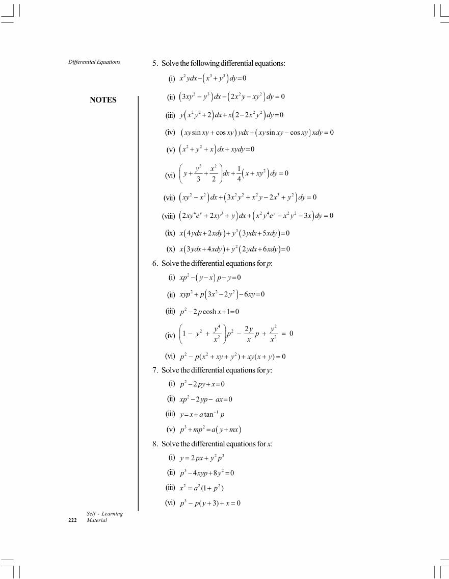
Differential Equations
NOTES
Self - Learning222 Material
5. Solve the following differential equations:
(i) 2 3 3 0x ydx x y dy
(ii) 2 3 2 23 2 0xy y dx x y xy dy
(iii) 2 2 2 22 2 2 0y x y dx x x y dy
(iv) sin cos sin cos 0xy xy xy ydx xy xy xy xdy
(v) 2 2 0x y x dx xydy
(vi) 3 2
210
3 2 4
y xy dx x xy dy
(vii) 2 2 2 2 2 3 23 2 0xy x dx x y x y x y dy
(viii) 4 3 2 4 2 22 2 3 0y yxy e xy y dx x y e x y x dy
(ix) 34 2 3 5 0x ydx xdy y ydx xdy
(x) 23 4 2 6 0x ydx xdy y ydx xdy
6. Solve the differential equations for p:
(i) 2 0xp y x p y
(ii) 2 2 23 2 6 0xyp p x y xy
(iii) 2 2 cosh 1 0p p x
(iv)4 2
2 22 2
21 0
y y yy p p
x x x
(vi) 2 2 2( ) ( ) 0p p x xy y xy x y
7. Solve the differential equations for y:
(i) 2 2 0p py x
(ii) 2 2 0xp yp ax
(iii) 1tany x a p
(v) 3 2p mp a y mx
8. Solve the differential equations for x:
(i) 2 32y px y p
(ii) 3 24 8 0p xyp y
(iii) 2 2 2(1 )x a p
(vi) 3 ( 3) 0p p y x
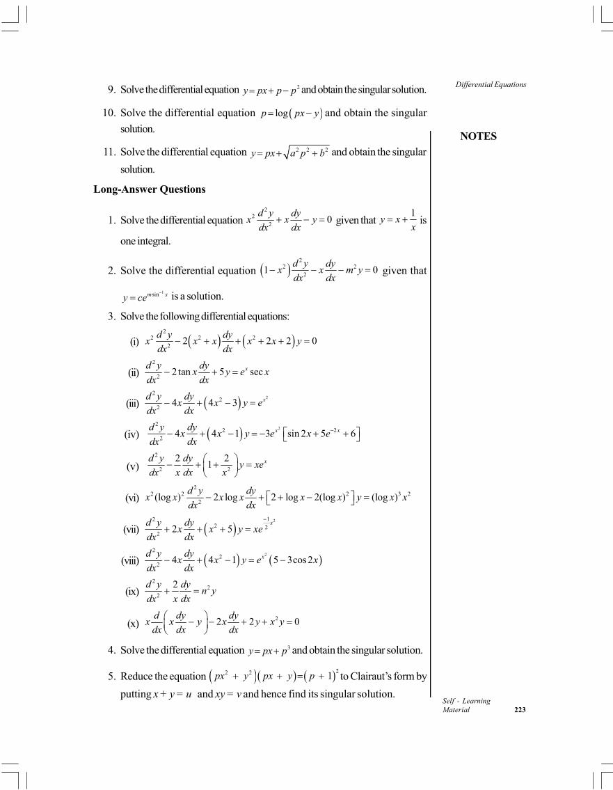
NOTES
Differential Equations
Self - LearningMaterial 223
9. Solve the differential equation 2y px p p and obtain the singular solution.
10. Solve the differential equation logp px y and obtain the singular
solution.
11. Solve the differential equation 2 2 2y px a p b and obtain the singular
solution.
Long-Answer Questions
1. Solve the differential equation 2
22
0d y dy
x x ydx dx
given that 1
y xx
is
one integral.
2. Solve the differential equation 2
2 22
1 0d y dy
x x m ydx dx
given that
1sinm xy ce
is a solution.
3. Solve the following differential equations:
(i) 2
2 2 22
2 2 2 0d y dy
x x x x x ydx dx
(ii)2
22 tan 5 secxd y dy
x y e xdx dx
(iii) 22
22
4 4 3 xd y dyx x y e
dx dx
(iv) 22
2 22
4 4 1 3 sin 2 5 6x xd y dyx x y e x e
dx dx
(v) 2
2 2
2 21 xd y dy
y xedx x dx x
(vi)2
2 2 2 3 22
(log ) 2 log 2 log 2(log ) (log )d y dy
x x x x x x y x xdx dx
(vii) 212
2 22
2 5xd y dy
x x y xedx dx
(viii) 22
22
4 4 1 5 3cos2xd y dyx x y e x
dx dx
(ix)2
22
2d y dyn y
dx x dx
(x)22 2 0
d dy dyx x y x y x y
dx dx dx
4. Solve the differential equation 3y px p and obtain the singular solution.
5. Reduce the equation 22 2 1px y px y p to Clairaut’s form by
putting x + y = u and xy = v and hence find its singular solution.
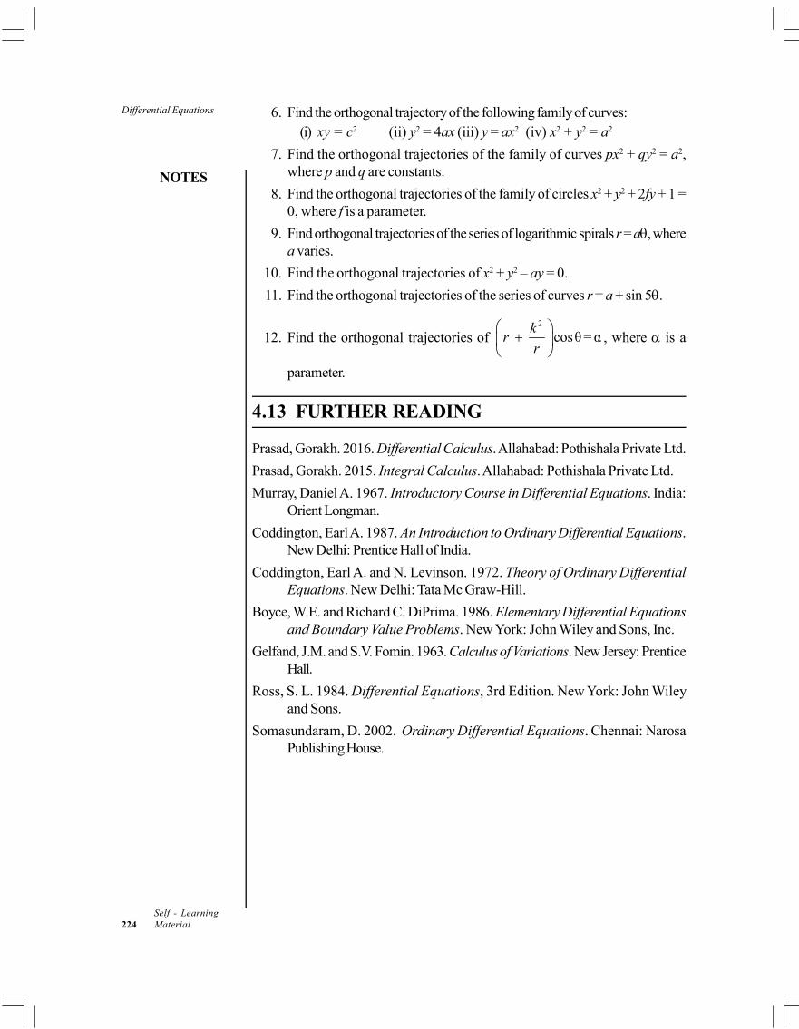
Differential Equations
NOTES
Self - Learning224 Material
6. Find the orthogonal trajectory of the following family of curves:(i) xy = c2 (ii) y2 = 4ax (iii) y = ax2 (iv) x2 + y2 = a2
7. Find the orthogonal trajectories of the family of curves px2 + qy2 = a2,where p and q are constants.
8. Find the orthogonal trajectories of the family of circles x2 + y2 + 2fy + 1 =0, where f is a parameter.
9. Find orthogonal trajectories of the series of logarithmic spirals r = a, wherea varies.
10. Find the orthogonal trajectories of x2 + y2 – ay = 0.
11. Find the orthogonal trajectories of the series of curves r = a + sin 5.
12. Find the orthogonal trajectories of 2
cosθ = αk
rr
, where is a
parameter.
4.13 FURTHER READING
Prasad, Gorakh. 2016. Differential Calculus. Allahabad: Pothishala Private Ltd.
Prasad, Gorakh. 2015. Integral Calculus. Allahabad: Pothishala Private Ltd.
Murray, Daniel A. 1967. Introductory Course in Differential Equations. India:Orient Longman.
Coddington, Earl A. 1987. An Introduction to Ordinary Differential Equations.New Delhi: Prentice Hall of India.
Coddington, Earl A. and N. Levinson. 1972. Theory of Ordinary DifferentialEquations. New Delhi: Tata Mc Graw-Hill.
Boyce, W.E. and Richard C. DiPrima. 1986. Elementary Differential Equationsand Boundary Value Problems. New York: John Wiley and Sons, Inc.
Gelfand, J.M. and S.V. Fomin. 1963. Calculus of Variations. New Jersey: PrenticeHall.
Ross, S. L. 1984. Differential Equations, 3rd Edition. New York: John Wileyand Sons.
Somasundaram, D. 2002. Ordinary Differential Equations. Chennai: NarosaPublishing House.
NOTES
Linear Differential Equationsand Method of Variation of
Parameters
Self - LearningMaterial 225
UNIT 5 LINEAR DIFFERENTIALEQUATIONS AND METHOD OFVARIATION OF PARAMETERS
Structure
5.0 Introduction5.1 Objectives5.2 Linear Differential Equations with Constant Coefficients5.3 Homogeneous Linear Ordinary Differential Equations5.4 Linear Differential Equation of Second Order5.5 Method of Variation of Parameters5.6 Answers to ‘Check Your Progress’5.7 Summary5.8 Key Terms5.9 Self-Assessment Questions and Exercises
5.10 Further Reading
5.0 INTRODUCTION
In mathematics, a differential equation has constant coefficients if only constantfunctions appear as coefficients in the associated homogeneous equation. Thelinear differential equation or a system of linear equations is generally the associatedhomogeneous equations having constant coefficients which may be solved byquadrature (mathematics), which means that the solutions may be expressed interms of integrals.
A homogeneous linear ordinary differential equation with constant coefficientsis an ordinary differential equation in which coefficients are constants (not functions),i.e., all terms are linear, and the entire differential equation is equal to zero, i.e., it isa homogeneous equation. Basically, a differential equation is homogeneous if it is ahomogeneous function of the unknown function and its derivatives. In the case oflinear differential equations, this means that there are no constant terms. The solutionsof any linear ordinary differential equation of any order may be deduced byintegration from the solution of the homogeneous equation obtained by removingthe constant term. The general solution of the homogeneous differential equationdepends on the roots of the characteristic quadratic equation.
The differential equations may contain one independent variable and two ormore than two dependent variables. The equation may be ordinary or partialdepending upon the ordinary or partial derivatives. To solve such equations, youwill require as many numbers of simultaneous differential equations as are thenumber of dependent variables.
Linear Differential Equationsand Method of Variation ofParameters
NOTES
Self - Learning226 Material
In mathematics, variation of parameters, also known as variation of constants,is a general method to solve inhomogeneous linear ordinary differential equations.For first order inhomogeneous linear differential equations, it is usually possible tofind solutions through integrating factors or undetermined coefficients withconsiderably less effort, although those methods leverage heuristics that involveguessing and is not appropriate for all inhomogeneous linear differential equations.
In this unit, you will study about the linear differential equations with constantcoefficients, homogeneous linear ordinary differential equations, linear differentialequation of second order, transformation of equations by changing the dependentvariable and the independent variable, and method of variation of parameters.
5.1 OBJECTIVES
After going through this unit, you will be able to:
Discuss about the linear differential equations with constant coefficients
Understand the various theorems related to linear differential equations
Solve simultaneous linear differential equations with constant coefficients
Define what homogeneous linear ordinary differential equations are
Reduce a homogeneous linear equation into a linear equation with constantcoefficients
Reduce a linear differential equation to a homogeneous linear equation
Explain the characteristics of linear differential equation of second order
Solve a linear differential equation of second order
Analyse the transformation of equations by changing the dependent variableand the independent variable
Elaborate on the method of variation of parameters
5.2 LINEAR DIFFERENTIAL EQUATIONSWITH CONSTANT COEFFICIENTS
In mathematics, an Ordinary Differential Equation (ODE) is a differential equationcontaining one or more functions of one independent variable and the derivativesof those functions. Basically, an ordinary differential equation is a relation thatcontains function of only one independent variable, and one or more of than twodependent variables. The equation may be ordinary or partial depending upon theordinary or partial derivatives. To solve such equations, you will require as manynumbers of simultaneous differential equations as are the number of dependentvariables.
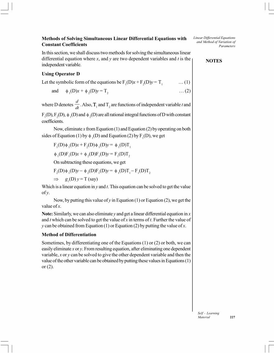
NOTES
Linear Differential Equationsand Method of Variation of
Parameters
Self - LearningMaterial 227
Methods of Solving Simultaneous Linear Differential Equations withConstant Coefficients
In this section, we shall discuss two methods for solving the simultaneous lineardifferential equation where x, and y are two dependent variables and t is theindependent variable.
Using Operator D
Let the symbolic form of the equations be F1(D)x + F
2(D)y = T
1 … (1)
and 1(D)x +
2(D)y = T
2 … (2)
where D denotes d
dt. Also, TT
1 and T
2 are functions of independent variable t and
F1(D), F
2(D),
1(D) and
2(D) are all rational integral functions of D with constant
coefficients.
Now, eliminate x from Equation (1) and Equation (2) by operating on bothsides of Equation (1) by
1(D) and Equation (2) by F
1(D), we get
F1(D)
1(D)x + F
2(D)
1(D)y =
1(D)T
1
1(D)F
1(D)x +
2(D)F
1(D)y = F
1(D)T
2
On subtracting these equations, we get
F2(D)
1(D)y
2(D)F
1(D)y =
1(D)T
1 F
1(D)T
2
g1(D) y = T (say)
Which is a linear equation in y and t. This equation can be solved to get the valueof y.
Now, by putting this value of y in Equation (1) or Equation (2), we get thevalue of x.
Note: Similarly, we can also eliminate y and get a linear differential equation in xand t which can be solved to get the value of x in terms of t. Further the value ofy can be obtained from Equation (1) or Equation (2) by putting the value of x.
Method of Differentiation
Sometimes, by differentiating one of the Equations (1) or (2) or both, we caneasily eliminate x or y. From resulting equation, after eliminating one dependentvariable, x or y can be solved to give the other dependent variable and then thevalue of the other variable can be obtained by putting these values in Equations (1)or (2).
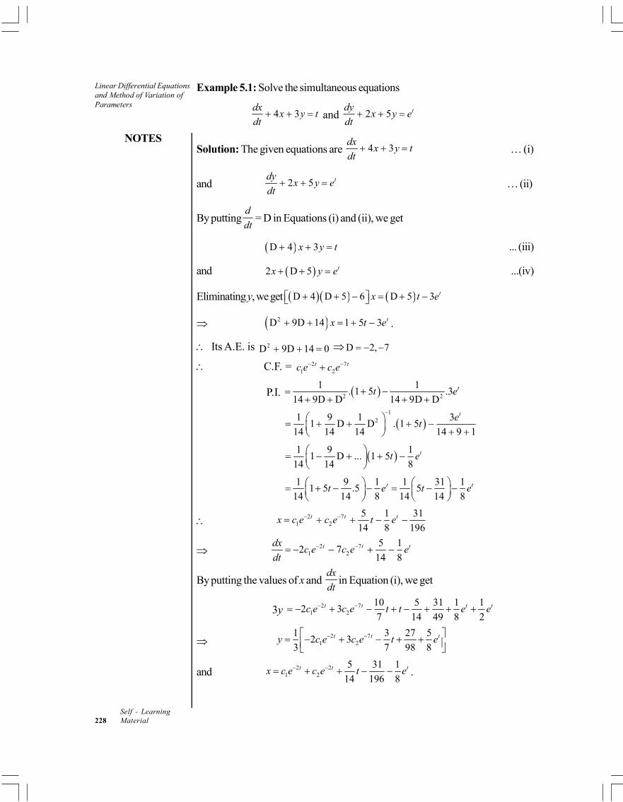
Linear Differential Equationsand Method of Variation ofParameters
NOTES
Self - Learning228 Material
Example 5.1: Solve the simultaneous equations
4 3dx
x y tdt
and 2 5 tdyx y e
dt
Solution: The given equations are 4 3dx
x y tdt
… (i)
and 2 5 tdyx y e
dt … (ii)
By puttingd
dt= D in Equations (i) and (ii), we get
D 4 3x y t ... (iii)
and 2 D 5 tx y e ...(iv)
Eliminating y, we get D 4 D 5 6 D 5 3 tx t e
2D 9D 14 1 5 3 tx t e .
Its A.E. is 2D 9D 14 0 D 2, 7
C.F. = 2 71 2
t tc e c e
P.I. 2 2
1 1. 1 5 .3
14 9D D 14 9D Dtt e
1
21 9 1 31 D D . 1 5
14 14 14 14 9 1
tet
1 9 11 D ... 1 5
14 14 8tt e
1 9 1 1 31 1
1 5 .5 514 14 8 14 14 8
t tt e t e
2 71 2
5 1 31
14 8 196t t tx c e c e t e
2 71 2
5 12 7
14 8t t tdx
c e c e edt
By putting the values of x and dx
dtin Equation (i), we get
3y 2 71 2
10 5 31 1 12 3
7 14 49 8 2t t t tc e c e t t e e
2 71 2
1 3 27 52 3
3 7 98 8t t ty c e c e t e
and 2 21 2
5 31 1
14 196 8t t tx c e c e t e .
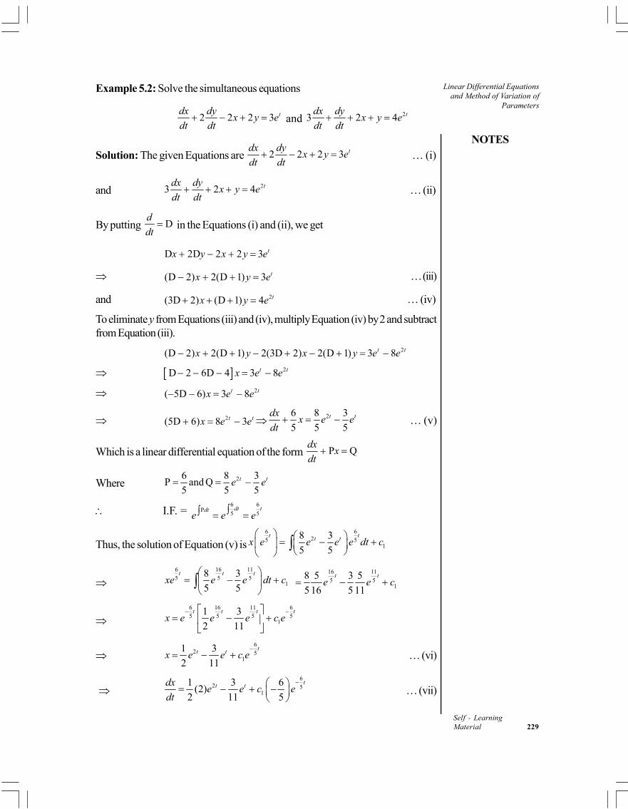
NOTES
Linear Differential Equationsand Method of Variation of
Parameters
Self - LearningMaterial 229
Example 5.2: Solve the simultaneous equations
2 2 2 3 tdx dyx y e
dt dt and 23 2 4 tdx dy
x y edt dt
Solution: The given Equations are 2 2 2 3 tdx dyx y e
dt dt … (i)
and 23 2 4 tdx dyx y e
dt dt … (ii)
By putting Dd
dt in the Equations (i) and (ii), we get
D 2D 2 2 3 tx y x y e
(D 2) 2(D 1) 3 tx y e … (iii)
and 2(3D 2) (D 1) 4 tx y e … (iv)
To eliminate y from Equations (iii) and (iv), multiply Equation (iv) by 2 and subtractfrom Equation (iii).
2(D 2) 2(D 1) 2(3D 2) 2(D 1) 3 8t tx y x y e e
2D 2 6D 4 3 8t tx e e
2( 5D 6) 3 8t tx e e
2(5D 6) 8 3t tx e e 26 8 3
5 5 5t tdx
x e edt
… (v)
Which is a linear differential equation of the form P Qdx
xdt
Where 26 8 3P and Q
5 5 5t te e
I.F. = 6 6
P5 5
dt tdte e e
Thus, the solution of Equation (v) is6 6
25 51
8 3
5 5
t tt tx e e e e dt c
6 16 11
5 5 51
8 3
5 5
t t txe e e dt c
16 11
5 51
8 5 3 5
5 16 5 11
t te e c
6 16 11 6
5 5 5 51
1 3
2 11
t t t tx e e e c e
6
2 51
1 3
2 11
tt tx e e c e
… (vi)
6
2 51
1 3 6(2)
2 11 5
tt tdxe e c e
dt
… (vii)
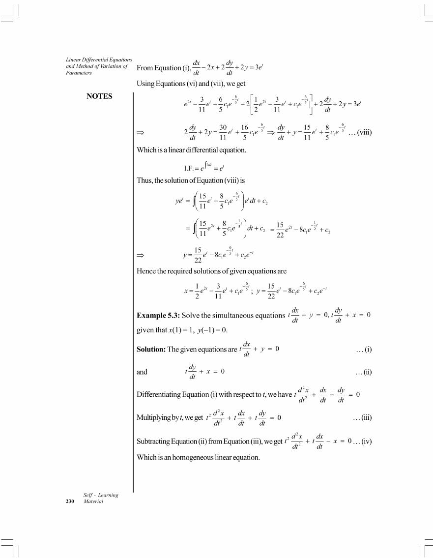
Linear Differential Equationsand Method of Variation ofParameters
NOTES
Self - Learning230 Material
From Equation (i), 2 2 2 3 tdx dyx y e
dt dt
Using Equations (vi) and (vii), we get
6 62 25 5
1 1
3 6 1 32 2 2 3
11 5 2 11
t tt t t t tdye e c e e e c e y e
dt
6
51
30 162 2
11 5
ttdy
y e c edt
6
51
15 8
11 5
ttdy
y e c edt
… (viii)
Which is a linear differential equation.
1I.F.
dt te e
Thus, the solution of Equation (viii) is
6
51 2
15 8
11 5
tt t tye e c e e dt c
1
2 51 2
15 8
11 5
tte c e dt c
12 5
1 2
158
22
tte c e c
6
51 2
158
22
tt ty e c e c e
Hence the required solutions of given equations are
62 5
1
1 3
2 11
tt tx e e c e
; 6
51 2
158
22
tt ty e c e c e
Example 5.3: Solve the simultaneous equations 0, 0dx dy
t y t xdt dt
given that x(1) = 1, y(–1) = 0.
Solution: The given equations are 0dx
t ydt
… (i)
and 0dy
t xdt
… (ii)
Differentiating Equation (i) with respect to t, we have2
20
d x dx dyt
dt dt dt
Multiplying by t, we get 2
22
0d x dx dy
t t tdt dt dt
… (iii)
Subtracting Equation (ii) from Equation (iii), we get2
22
0d x dx
t t xdt dt
… (iv)
Which is an homogeneous linear equation.
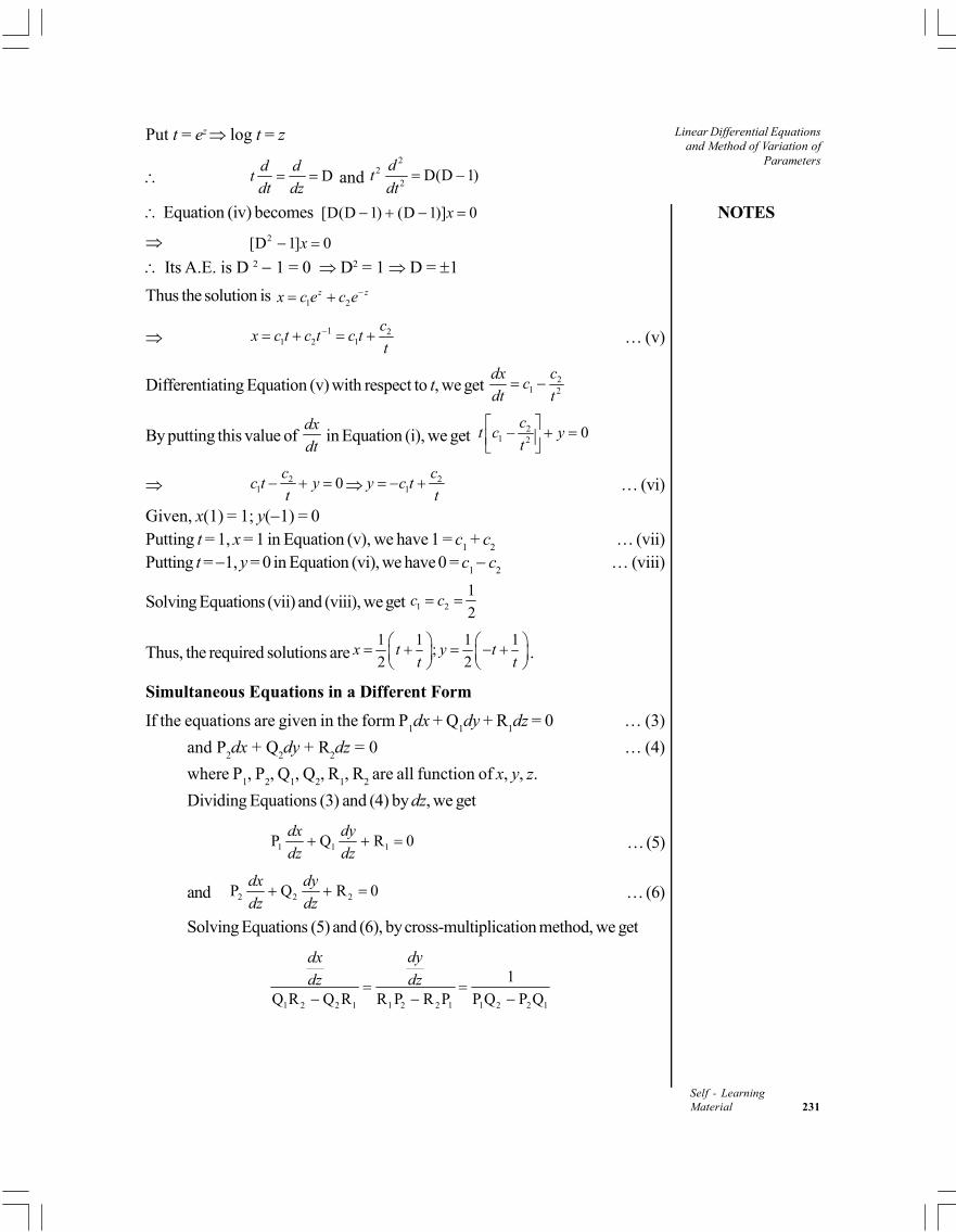
NOTES
Linear Differential Equationsand Method of Variation of
Parameters
Self - LearningMaterial 231
Put t = ez log t = z
Dd d
tdt dz
and 2
2
2D(D 1)
dt
dt
Equation (iv) becomes [D(D 1) (D 1)] 0x
2[D 1] 0x
Its A.E. is D 2 1 = 0 D2 = 1 D = 1
Thus the solution is 1 2z zx c e c e
1 21 2 1
cx c t c t c t
t … (v)
Differentiating Equation (v) with respect to t, we get 21 2
cdxc
dt t
By putting this value of dx
dt in Equation (i), we get 2
1 20
ct c y
t
21 0
cc t y
t 2
1
cy c t
t … (vi)
Given, x(1) = 1; y(1) = 0Putting t = 1, x = 1 in Equation (v), we have 1 = c
1 + c
2… (vii)
Putting t = 1, y = 0 in Equation (vi), we have 0 = c1 c
2… (viii)
Solving Equations (vii) and (viii), we get 1 2
1
2c c
Thus, the required solutions are1 1 1 1
;2 2
x t y tt t
.
Simultaneous Equations in a Different Form
If the equations are given in the form P1dx + Q
1dy + R
1dz = 0 … (3)
and P2dx + Q
2dy + R
2dz = 0 … (4)
where P1, P
2, Q
1, Q
2, R
1, R
2 are all function of x, y, z.
Dividing Equations (3) and (4) by dz, we get
1 1 1P Q R 0dydx
dz dz … (5)
and 2 2 2P Q R 0dydx
dz dz … (6)
Solving Equations (5) and (6), by cross-multiplication method, we get
1 2 2 1 1 2 2 1 1 2 2 1
1
Q R Q R R P R P P Q P Q
dydx
dz dz
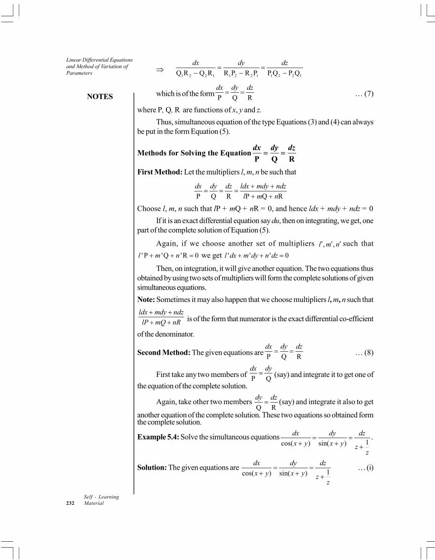
Linear Differential Equationsand Method of Variation ofParameters
NOTES
Self - Learning232 Material
1 2 2 1 1 2 2 1 1 2 2 1Q R Q R R P R P P Q P Q
dydx dz
which is of the form P Q R
dydx dz … (7)
where P, Q, R are functions of x, y and z.
Thus, simultaneous equation of the type Equations (3) and (4) can alwaysbe put in the form Equation (5).
Methods for Solving the EquationP Q R
dx dy dz
First Method: Let the multipliers l, m, n be such that
P Q R P Q R
dy ldx mdy ndzdx dz
l m n
Choose l, m, n such that lP + mQ + nR = 0, and hence ldx + mdy + ndz = 0
If it is an exact differential equation say du, then on integrating, we get, onepart of the complete solution of Equation (5).
Again, if we choose another set of multipliers , ,l m n such that
' P 'Q 'R 0l m n we get ' ' ' 0l dx m dy n dz
Then, on integration, it will give another equation. The two equations thusobtained by using two sets of multipliers will form the complete solutions of givensimultaneous equations.
Note: Sometimes it may also happen that we choose multipliers l, m, n such that
ldx mdy ndz
lP mQ nR
is of the form that numerator is the exact differential co-efficient
of the denominator.
Second Method: The given equations are P Q R
dydx dz … (8)
First take any two members of P Q
dydx (say) and integrate it to get one of
the equation of the complete solution.
Again, take other two members Q R
dy dz (say) and integrate it also to get
another equation of the complete solution. These two equations so obtained formthe complete solution.
Example 5.4: Solve the simultaneous equations1cos( ) sin( )
dx dy dz
x y x y zz
.
Solution: The given equations are 1cos( ) sin( )
dx dy dz
x y x y zz
… (i)

NOTES
Linear Differential Equationsand Method of Variation of
Parameters
Self - LearningMaterial 233
Choosing 1, 1, 0 as multipliers, we get
1cos( ) sin( )
dx dy dz
x y x y zz
cos( ) sin( )
dx dy
x y x y
2 1 sin( ) cos( )
zdz dx dy
z x y x y
2
2 ( )
2( 1)2 sin
4
zdz d x y
zx y
2
1 2cosec ( ) ( )
1 42
zdzx y d x y
z
Integrating both sides, we get
21
1 1log( 1) log tan ( ) log
2 42z x y c
2 1/ 21log( 1) log tan log
2 8
x yz c
2 1/ 2
1
( 1)log log
tan2 8
zc
x y
2 1 / 2
1
( 1)
tan2 8
zc
x y
… (ii)
Now, choosing 1, 1, 0 and 1, 1, 0 as multipliers in Equation (i), we get
cos( ) sin( ) cos( ) sin( )
dx dy dx dy
x y x y x y x y
cos( ) sin( )
( )cos( ) sin( )
x y x ydx dy dx dy
x y x y
cos( ) sin( )
( ) ( )sin( ) cos( )
x y x yd x y d x y
x y x y
Integrating both sides, we have 2log sin( ) cos( ) logx y x y x y c
2log sin( ) cos( ) ( ) logx y x y y x c
2log sin( ) cos( ) logy xx y x y e c
2sin( ) cos( ) y xx y x y e c … (iii)
Thus, Equations (ii) and (iii) together form the complete solution of the givenequations.
Example 5.5: Solve the simultaneous equations2 22
xdx dy dz
z yz y y z y z
.
Solution: The given equations are 2 22
xdx dy dz
z yz y y z y z
… (i)
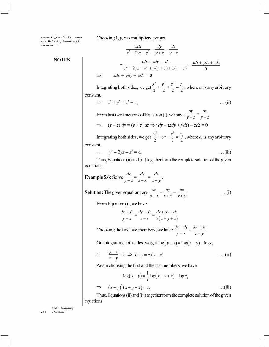
Linear Differential Equationsand Method of Variation ofParameters
NOTES
Self - Learning234 Material
Choosing 1, y, z as multipliers, we get
2 22
xdx dy dz
z yz y y z y z
2 22 ( ) ( )
xdx ydy zdz
z yz y y y z z y z
0
xdx ydy zdz
xdx + ydy + zdz = 0
Integrating both sides, we get2 2 2
1
2 2 2 2
cx y z , where c
1 is any arbitrary
constant.
x2 + y2 + z2 = c1
… (ii)
From last two fractions of Equation (i), we have dy dz
y z y z
(y z) dy = (y + z) dz ydy (zdy + ydz) zdz = 0
Integrating both sides, we get 2 2
2
2 2 2
cy zyz , where c
2 is any arbitrary
constant.
y2 2yz z2 = c2
… (iii)
Thus, Equations (ii) and (iii) together form the complete solution of the givenequations.
Example 5.6: Solvedx dy dz
y z z x x y
.
Solution: The given equations are dx dy dz
y z z x x y
… (i)
From Equation (i), we have
2
dx dy dy dz dx dy dz
y x z y x y z
Choosing the first two members, we have dx dy dy dz
y x z y
On integrating both sides, we get 1log log logy x z y c
1
y xc
z y
1( )x y c y z … (ii)
Again choosing the first and the last members, we have
2
1log log log
2x y x y z c
2
2x y x y z c …(iii)
Thus, Equations (ii) and (iii) together form the complete solution of the givenequations.
NOTES
Linear Differential Equationsand Method of Variation of
Parameters
Self - LearningMaterial 235
Check Your ProgressSolving the following equations:
1. 7 0dx
x ydt
and 2 5 0dy
x ydt
.
2. 5 tdxx y e
dt and 23 tdy
x y edt
3. 2 , 2 , 2dx dy dz
y z xdt dt dt
.
4. ( ) ( ) ( )
adx bdy cdz
b c yz c a zx a b xy
5. 3 4 4 3 3 32 2 9 ( )
dx dy dz
y x x y x y z x y
6. ( )
dx dy dz
x y x y z
7. 2 2 2 2 2
dx dy dz
y x x y z
5.3 HOMOGENEOUS LINEAR ORDINARYDIFFERENTIAL EQUATIONS
Consider the following differential equations:
1.2
22
4 2 xd y dyx x y e
dx dx
2.3
33
(2 1) (2 1) 2 0d y dy
x x ydx dx
3.2
22 2 xd y dy
x x y edx dx
All these differential equations are linear since the dependent variable y andits derivatives occur only in the first degree and are not multiplied together. In thefirst equation the powers of x are same as the order of the derivatives associatedwith them. Such equations are called homogeneous linear equations. The secondequation in the given form is not homogeneous but can be changed to homogeneousby replacing 2x – 1 with X. The third equation is linear but it not homogeneous.
Homogeneous linear equation is an equation of the form1
10 1 1
P P ... P Xn n
n nnn n
d y d yx x y
dx dx
where P0, P
1, P
2, …, P
n are constants and X is either a constant or a function of x.
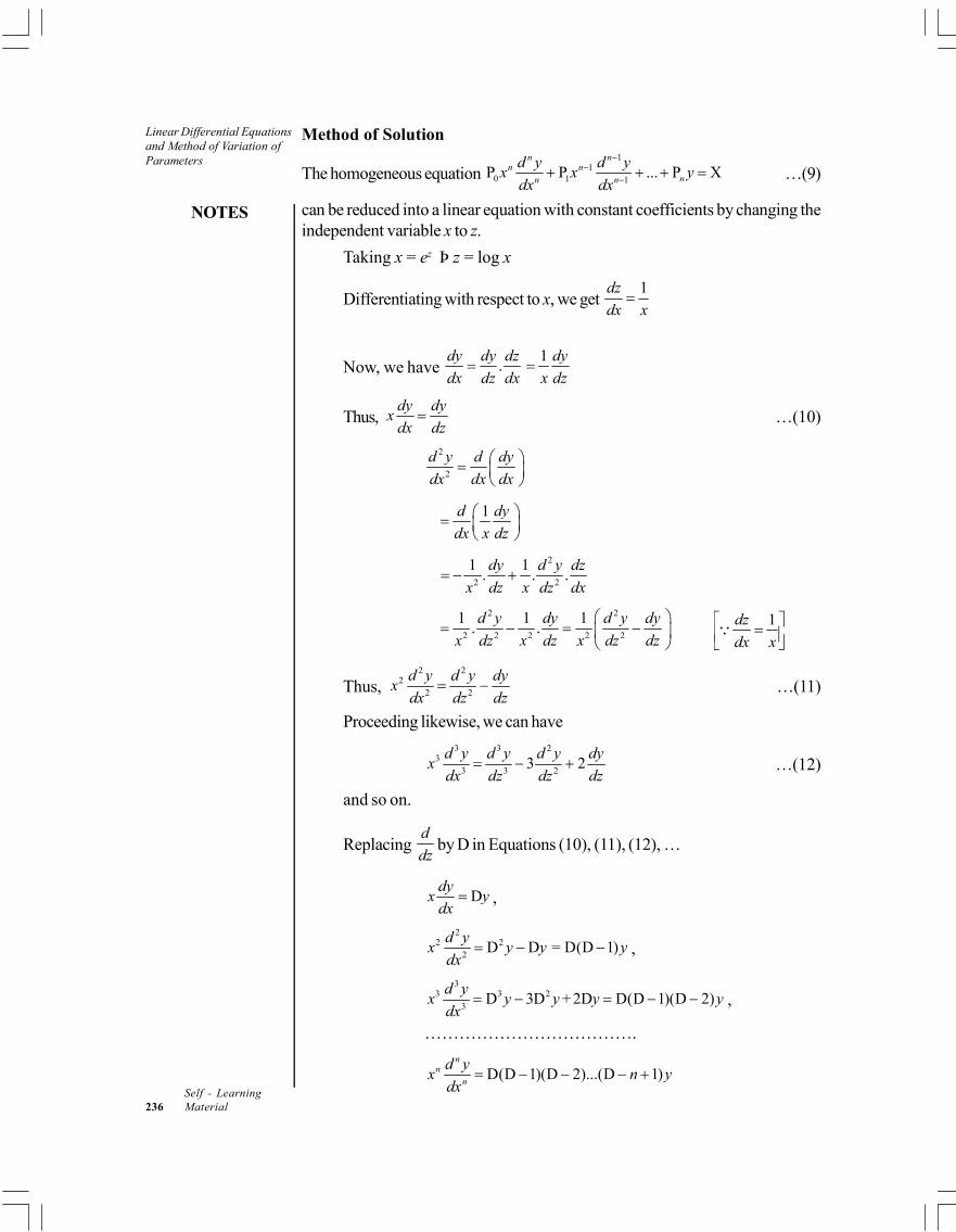
Linear Differential Equationsand Method of Variation ofParameters
NOTES
Self - Learning236 Material
Method of Solution
The homogeneous equation 1
10 1 1
P P ... P Xn n
n nnn n
d y d yx x y
dx dx
…(9)
can be reduced into a linear equation with constant coefficients by changing theindependent variable x to z.
Taking x = ez Þ z = log x
Differentiating with respect to x, we get 1dz
dx x
Now, we have .dy dy dz
dx dz dx
1 dy
x dz
Thus,dy dy
xdx dz
…(10)
2
2
d y d dy
dx dx dx
1d dy
dx x dz
2
2 2
1 1. . .dy d y dz
x dz x dz dx
2 2
2 2 2 2 2
1 1 1. .d y dy d y dy
x dz x dz x dz dz
1dz
dx x
Thus, 2 2
22 2
d y d y dyx
dx dz dz …(11)
Proceeding likewise, we can have
3 3 23
3 3 23 2
d y d y d y dyx
dx dz dz dz …(12)
and so on.
Replacing d
dzby D in Equations (10), (11), (12), …
Ddy
x ydx
,
22 2
2D D = D(D 1)
d yx y y y
dx ,
33 3 2
3D 3D + 2D D(D 1)(D 2)
d yx y y y y
dx ,
……………………………….
D(D 1)(D 2)...(D 1)n
nn
d yx n y
dx
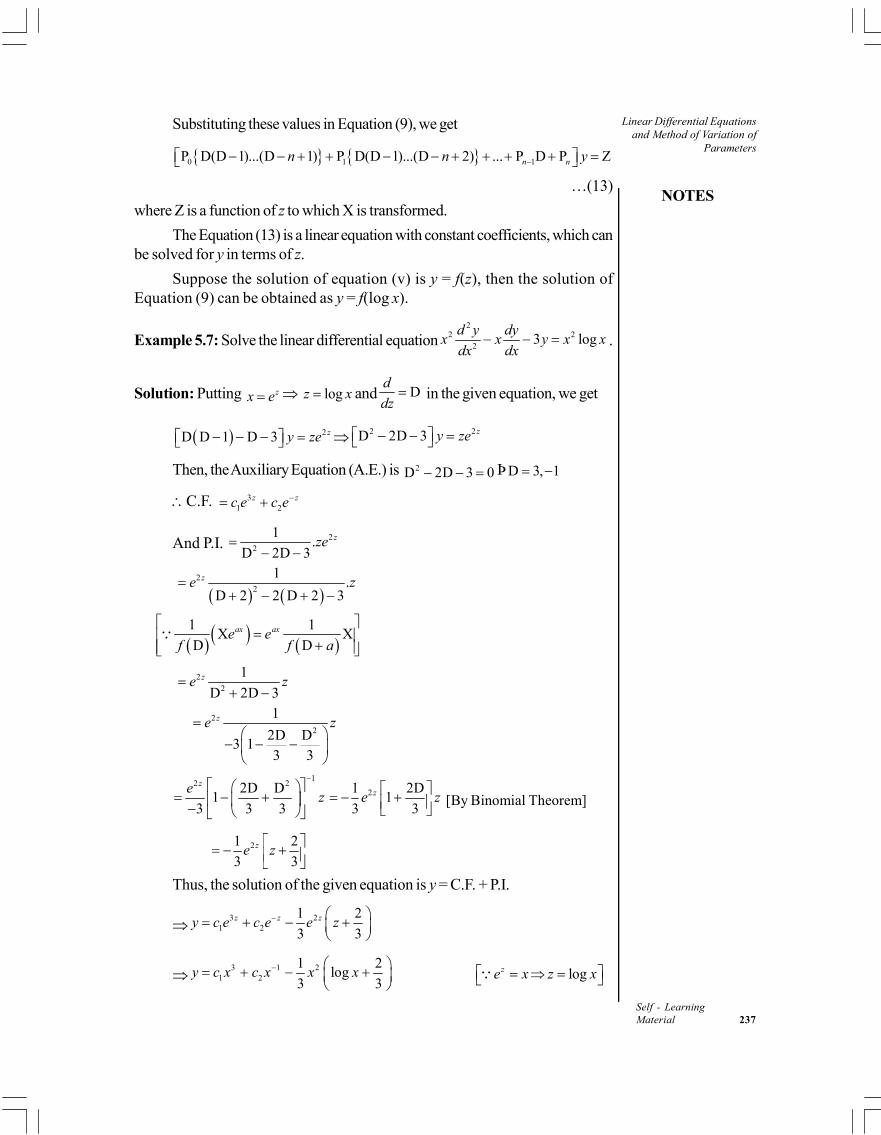
NOTES
Linear Differential Equationsand Method of Variation of
Parameters
Self - LearningMaterial 237
Substituting these values in Equation (9), we get
0 1 1P D(D 1)...(D 1) P D(D 1)...(D 2) ... P D P Zn nn n y
…(13)
where Z is a function of z to which X is transformed.
The Equation (13) is a linear equation with constant coefficients, which canbe solved for y in terms of z.
Suppose the solution of equation (v) is y = f(z), then the solution ofEquation (9) can be obtained as y = f(log x).
Example 5.7: Solve the linear differential equation2
2 22
3 logd y dy
x x y x xdx dx
.
Solution: Putting zx e logz x and Dd
dz in the given equation, we get
2D D 1 D 3 zy ze 2 2D 2D 3 zy ze
Then, the Auxiliary Equation (A.E.) is 2D 2D 3 0 Þ D 3, 1
C.F. 31 2
z zc e c e
And P.I. 22
1.
D 2D 3zze
2
2
1.
D 2 2 D 2 3ze z
1 1
X XD D
ax axe ef f a
2
2
1
D 2D 3ze z
2
2
1
2D D3 1
3 3
ze z
12 22D D
13 3 3
zez
21 2D1
3 3ze z
[By Binomial Theorem]
21 2
3 3ze z
Thus, the solution of the given equation is y = C.F. + P.I.
3 21 2
1 2
3 3z z zy c e c e e z
3 1 21 2
1 2log
3 3y c x c x x x
logze x z x
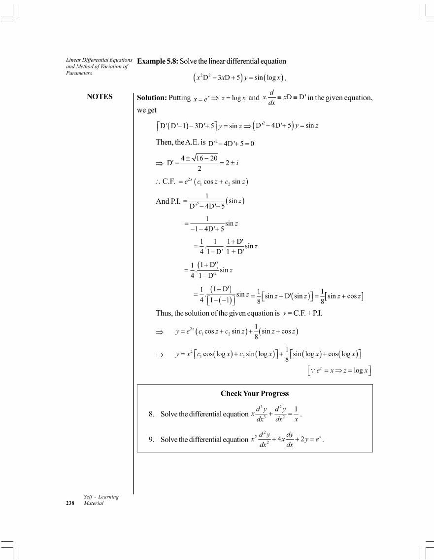
Linear Differential Equationsand Method of Variation ofParameters
NOTES
Self - Learning238 Material
Example 5.8: Solve the linear differential equation
2 2D 3 D 5 sin logx x y x .
Solution: Putting zx e logz x and . D D'd
x xdx
in the given equation,
we get
D' D' 1 3D' 5 siny z 2D' 4D' 5 siny z
Then, the A.E. is 2D' 4D' 5 0
4 16 20
D = 22
i
C.F. 21 2cos sinxe c z c z
And P.I. 2
1sin
D' 4D' 5z
1
sin1 4D' 5
z
1 1 1 D'. . sin
4 1 D' 1 + D'z
2
1 D'1. sin
4 1 D'z
1 D'1. sin
4 1 1z
1 1
sin D' sin sin cos8 8
z z z z
Thus, the solution of the given equation is y C.F. + P.I.
21 2
1cos sin sin cos
8zy e c z c z z z
21 2
1cos log sin log sin log cos log
8y x c x c x x x
logze x z x
Check Your Progress
8. Solve the differential equation 3 2
3 2
1d y d yx
dx dx x .
9. Solve the differential equation 2
22
4 2 xd y dyx x y e
dx dx .
NOTES
Linear Differential Equationsand Method of Variation of
Parameters
Self - LearningMaterial 239
5.4 LINEAR DIFFERENTIAL EQUATION OFSECOND ORDER
Linear Differential Equation of Second Order is an equation of the form
2
2P Q R
d y dyy
dx dx
where P, Q and R are the functions of x.
Solution by Changing the Dependent Variable when One IntegralBelonging to the C.F. is Known
Let the linear differential equation of second order be
2
2P Q R
d y dyy
dx dx ...(14)
where P, Q and R are the functions of x only.
Let y = u be a known integral belonging to the C.F. of the Equation (14).Thus, its solution is
2
2P Q 0
d y dyy
dx dx ...(15)
Taking y = uv and differentiating with respect to x, we get
1 1
dyu v uv
dx and
2
2 1 1 222
d yu v u v uv
dx
Putting these values in Equation (14), we get
2 1 1 2 1 12 P Q Ru v u v uv u v uv uv
2 1 1 2 12 P P Q Ruv u u v u u u v ...(16)
Since y = u is the solution of Equation (15), thus Equation (15) can bewritten as
2 1P Q 0u u u
Using this value in Equation (16), we get
2 1 12 P 0 Ruv u u v
2 1 1
2 RPv u v
u u
Now, putting 1v p and 2
dpv
dx , we get
1
2 RP
dpu p
dx u u
...(17)
This is a linear equation in p. Thus, its
I.F. = 12
Pu dxue
2P P P2log log 2. .dx dx dxu ue e e e u e
Linear Differential Equationsand Method of Variation ofParameters
NOTES
Self - Learning240 Material
Now, we have the solution of Equation (17) as
P P2 21
R. .
dx dxp u e u e dx c
u
P P P2 21R
dx dx dxp u e ue dx c u e
P P P2 21R
dx dx dxdvu e ue dx c u e
dx
dvp
dx
Integrating both sides, we get
P P P2 21 2R
dx dx dxv u e ue dx dx c u e dx c
The complete solution of Equation (14) is given by y = uv
P P P2 21 2R
dx dx dxy u u e ue dx dx c u u e dx c u
Where c1 and c
2 are two arbitrary constants.
Determining the particular integral of 2
2P Q 0
d y dyy
dx dx
In case the integral of C.F. is not known while solving linear differential equationsof second degree, one of the following rules helps us in finding the particular integralof
2
2P Q 0
d y dyy
dx dx ...(18)
Rule 1: Let mxy e be the solution of Equation (18).
Differentiating with respect to x, we get
mxdyme
dx and
22
2mxd y
m edx
Putting these values in Equation (18), we get2 P Q 0mx mx mxm e me e
2 P Q 0mxm m e
2 P Q = 0m m
Thus, mxy e is the solution of Equation (18) if 2 P Q = 0m m .
Corollary: Taking m = 1, y = ex is a solution of Equation (18) if1 + P + Q = 0 .
Taking m = –1, y = e–x is a solution of Equation (18) if 1 – P + Q = 0.
Taking m = a, y = eax is a solution of Equation (18) if a2 + aP + Q = 0.
Rule 2: Let my x be the solution of Equation (18).
NOTES
Linear Differential Equationsand Method of Variation of
Parameters
Self - LearningMaterial 241
Differentiating both sides with respect to x, we get
1mdymx
dx and
22
2( 1) md y
m m xdx
Putting these values in Equation (18), we get
2 1( 1) P Q 0m m mm m x mx x
2( 1) P Q 0m m mx x
Thus, my x is the solution of Equation (18) if 2( 1) P Q 0m m mx x .
Corollary: Taking m = 1, y = x is a solution of Equation (18) if P + Qx = 0.
Taking m = 2, y = x2 is a solution of Equation (18) if 2 + 2Px +Qx2 = 0.
Example 5.9: Solve the differential equation
2
2cot 1 cot sin .xd y dy
x x y e xdx dx
Solution: The given differential equation is
2
2cot 1 cot sinxd y dy
x x y e xdx dx
... (i)
Comparing it with 2
2P Q R,
d y dyy
dx dx we get
P cot ,Q 1 cot ,R sinxx x e x
Now, P Q 1 cot 1 cot 1 0x x
Since P + Q + 1= 0, thus xy e is a part of C.F..
Taking xy ve ,
x xdy dve e v
dx dx and
2 2
2 22 .x x xd y d v dv
e e vedx dx dx
Substituting these values in Equation (i), we get
2
22 . cot 1 cot sinx x x x x x xd v dv dv
e e ve x e e v x ve e xdx dx dx
2
2+ 2 cot sin
d v dvx x
dx dx
2 cot sindp
x p xdx
where dv
pdx
and2
2
dp d v
dx dx ...(ii)
This is a linear differential equation in p, i.e., P ' Q 'dp
pdx
, where
P = 2 – cot x and Q = sin x. Thus, its I.F.
= P ' 2 cot 2 logsindx x dx x xe e e
2 2
logsin sin
x x
x
e e
e x
Linear Differential Equationsand Method of Variation ofParameters
NOTES
Self - Learning242 Material
Now, the solution of Equation (ii) is given by
p(I.F) 1Q'(I.F)dx c
2 2
1. sin .sin sin
x xe ep x dx c
x x
2 2
1.sin 2
x xe ep c
x
2
12 2
sin sin.
2
x
x x
e x xp c
e e
21
sinsin
2xdv x
c e xdx
dv
pdx
21
sinsin
2xx
dv c e x dx
Integrating both sides, we get 2
1
sinsin
2xx
dv c e x dx
2
12
cos2sin cos
2 5
xc exv x x c
Thus, the complete solution of Equation (i) is given by xy ve
12
1cos 2sin cos
2 5
xx xc e
y e x x x c e
Solution by Removing the First Derivative and Changing theDependent Variable
In case the integral of the C.F. is neither known nor can be found using the rules,there is a need of other method to find the solution of linear differential equation ofsecond order. Here, we will learn the method which is independent of integral ofC.F.
Consider the linear differential equation of second order
2
2P Q R
d y dyy
dx dx ...(19)
Change the dependent variable in the Equation (19) by putting y uv , whereu and v are the functions of x.
Now, dy dv du
u vdx dx dx
and 2 2 2
2 2 22 .
d y d v du dv d uu v
dx dx dx dx dx
Putting these values in Equation (19), we get
2 2
2 22 . P Q( ) R
d v du dv d u dv duu v u v uv
dx dx dx dx dx dx
NOTES
Linear Differential Equationsand Method of Variation of
Parameters
Self - LearningMaterial 243
2 2
2 2P 2 P Q R
d v du dv d u duu u u v
dx dx dx dx dx
2 2
2 2
2 1 P RP . . . Q
d v du dv d u duv
dx u dx dx u dx u dx u
...(20)
Taking u such that the coefficient of first derivative dv
dx = 0 (i.e., removing
first derivative from Equation (20)), we get
2P + 0
du
u dx
P =
2
dudx
u
Integrating both sides, we get
1 = P
2
dudx
u
1
log = P2
u dx
1
P2 =
dxu e
…(21)
Since 2
P + 0du
u dx , Equation (20) becomes
2 2
2 2
1 P R. . Q
d v d u duv
dx u dx u dx u
…(22)
From Equation (21),
1P
21 1
= P P2 2
dxdue u
dx
and 2
2 22
1 P P 1 1 P 1 1 P = P P
2 2 2 4 2
d u du d d du u u u u
dx dx dx dx dx
Putting these values in Equation (22), we get
12P2 2
2
1 1 1 P P 1P P Q R
4 2 2
dxd v du u u v e
dx u dx u
12
P2 2 22
1 1 P 1P P Q R
4 2 2
dxd v dv e
dx dx
12P2 2
2
1 P 1Q P R
2 4
dxd v dv e
dx dx
2
2P Q
d vv
dx ...(23)
where 1
P2 21 P 1
P = Q . P ,Q = R2 4
dxde
dx
The Equation (23) is called the normal form of the Equation (19).Equation (23) can easily be integrated and then can be solved for v.
Thus, the general solution of Equation (19) is y = uv, which contains twoarbitrary constants.
Linear Differential Equationsand Method of Variation ofParameters
NOTES
Self - Learning244 Material
Example 5.10: Solve the differential equation2 2cos cos 0
d dyx y x
dx dx
.
Solution: The given differential equation is 2 2cos cos 0
d dyx y x
dx dx
2
2 22
cos 2sin cos cos 0d y dy
x x x y xdx dx
2
22 tan 0
d y dyx y
dx dx ...(i)
Comparing Equation (i) with 2
2P Q R
d y dyy
dx dx , we get
P = –2 tan x, Q = 1 and R = 0Putting y uv in Equation (i), the equation is transformed into
2
2P' Q
d vv
dx ...(ii)
where1 1
P 2 tan logsec2 2 secdx x dx xu e e e x
2 21 P 1 1 1P ' Q P 1 2 tan 4 tan
2 4 2 4
d dx x
dx dx
2 2 2 21 sec tan 1 1 tan tan 2x x x x
and1
P2Q' R 0
dxe
Putting these values in Equation (ii), it gets transformed into 2
22 0
d vv
dx
…(iii)
Symbolic form of this equation is 2D 2 0v
Its auxiliary equation is 2D 2 0 2D 2 D 2i
Now, the solution of Equation (iii) is given by1 2cos 2 sin 2v c x c x
Thus, the solution of Equation (i) is given by y uv
1 2sec cos 2 sin 2y x c x c x
Solution by Changing the Independent Variable
Consider the linear differential equation of second degree
2
2P Q R
d y dyy
dx dx ...(24)
Changing the independent variable x to z with the help of relation z = f(x) ,we get
.dy dy dz
dx dz dx
NOTES
Linear Differential Equationsand Method of Variation of
Parameters
Self - LearningMaterial 245
2
2
d y d dy
dx dx dx
22 2
2 2. .
d dy dz d y dz dy d z
dx dz dx dz dx dz dx
Substituting these values in the Equation (24), we get22 2
2 2. P . Q R
d y dz dy d z dy dzy
dz dx dz dx dz dx
2
2 2
2 2 22
P Q Rd z dz
d y dy ydx dxdz dzdz dz dz
dx dx dx
2
1 1 12P Q R
d y dyy
dz dz ...(25)
where
2
2
1 1 12 2 2
P Q RP ,Q ,R
d z dz
dx dxdz dz dz
dx dx dx
Here, P1, Q
1 and R
1 are the functions of x but can be expressed as the
functions of z with the help of the relation between z and x.
1. Choosing z such that the Coefficient of P1 is Zero.
2
2
1 2
PP 0
d z dz
dx dxdz
dx
2
2P 0
d z dz
dx dx
2
2P
d z dz
dx dx
2
2
P
d z
dxdz
dx
Integrating both sides, we get
log Pdz
dxdx
Pdxdz
edx
Integrating again, we get Pdx
z e dx
For the relationPdx
z e dx
, P1 will be zero and Equation (25)
reduces to2
1 12Q R
d yy
dz ...(26)
Linear Differential Equationsand Method of Variation ofParameters
NOTES
Self - Learning246 Material
If Q1 is constant or a constant multiplied by 2
1
z, then Equation (26) can be
solved easily giving the value of y in terms of z. Then, by replacing z in terms of x,we get the general solution of Equation (24).
2. Choosing z such that the Coefficient of Q1 is Constant.
21Q a (say)
22
Qa
dz
dx
22 = Q
dza
dx
Qdz
adx
1
Qdz
dx a
Integrating both sides, we get
1
Qz dxa
For the relation1
Qz dxa
, Q1 = a2 and Equation (25) reduces to
2
21 12
P Rd y dy
a ydz dz
...(27)
If P1 is a constant, then Equation (27) can be solved easily giving the value
of y in terms of z. Then, by replacing z in terms of x, we get the general solution ofEquation (24).
Example 5.11: Solve the differential equation
2
2 cos 22
3sin cot 2 sin sinxd y dyx x y x e x
dx dx .
Solution: The given differential equation is
2
2 cos 22
3sin cot 2 sin sinxd y dyx x y x e x
dx dx ...(i)
Comparing it with 2
2P Q R
d y dyy
dx dx , we get
2P 3sin cot , Q 2sinx x x and cos 2R sinxe x
Let P 3sin cotdx x x dxdz
e edx
3cos logsin 3cossin .x x xe x e
Integrating, we get
3cos 3cos1sin 3sin
3x xz e x dx e x dx
3cos1
3xe
On changing the independent variable x to z by the relation 3cos1
3xz e ,
Equation (i) reduces to the form2
1 1 12P Q R
d y dyy
dz dz …(ii)
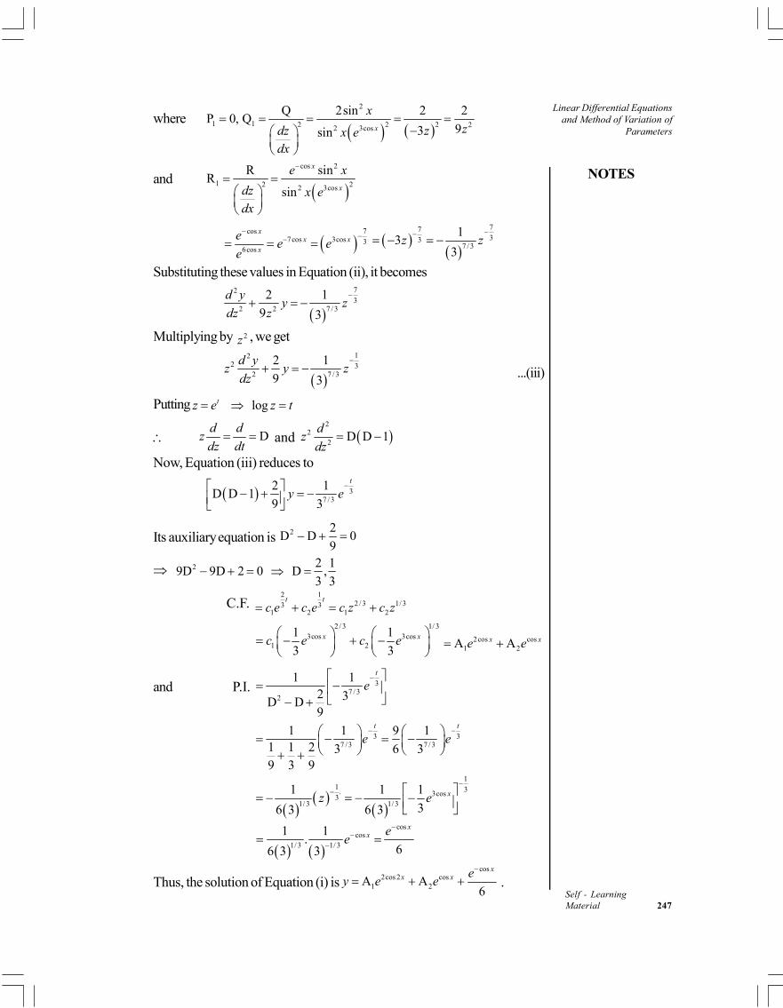
NOTES
Linear Differential Equationsand Method of Variation of
Parameters
Self - LearningMaterial 247
where
2
1 1 2 2 2 22 3cos
Q 2sin 2 2P 0, Q
93sin x
x
zzdz x edx
and
cos 2
1 2 22 3cos
R sinR
sin
x
x
e x
dz x edx
7cos
7cos 3cos 36cos
xx x
x
ee e
e
7733
7 / 3
13
3z z
Substituting these values in Equation (ii), it becomes
723
7 / 32 2
2 1
9 3
d yy z
dz z
Multiplying by 2z , we get
122 3
7 / 32
2 1
9 3
d yz y z
dz
...(iii)
Putting logtz e z t
Dd d
zdz dt
and 2
22
D D 1d
zdz
Now, Equation (iii) reduces to
37 / 3
2 1D D 1
9 3
t
y e
Its auxiliary equation is 2 2D D 0
9
2 2 19D 9D 2 0 D ,
3 3
C.F. 2 1
2 / 3 1/ 33 31 2 1 2
t tc e c e c z c z
2 / 3 1/ 3
3cos 3cos1 2
1 1
3 3x xc e c e
2cos cos1 2A Ax xe e
and P.I. 37 / 3
2
1 12 3D D9
t
e
3 3
7 /3 7 / 3
1 1 9 11 1 2 3 6 39 3 9
t t
e e
11 3. 3cos3
1/ 3 1/ 3
1 1 1
36 3 6 3xz e
coscos
1/ 3 1/ 3
1 1.
66 3 3
xx e
e
Thus, the solution of Equation (i) iscos
2cos 2 cos1 2A A
6
xx x e
y e e
.
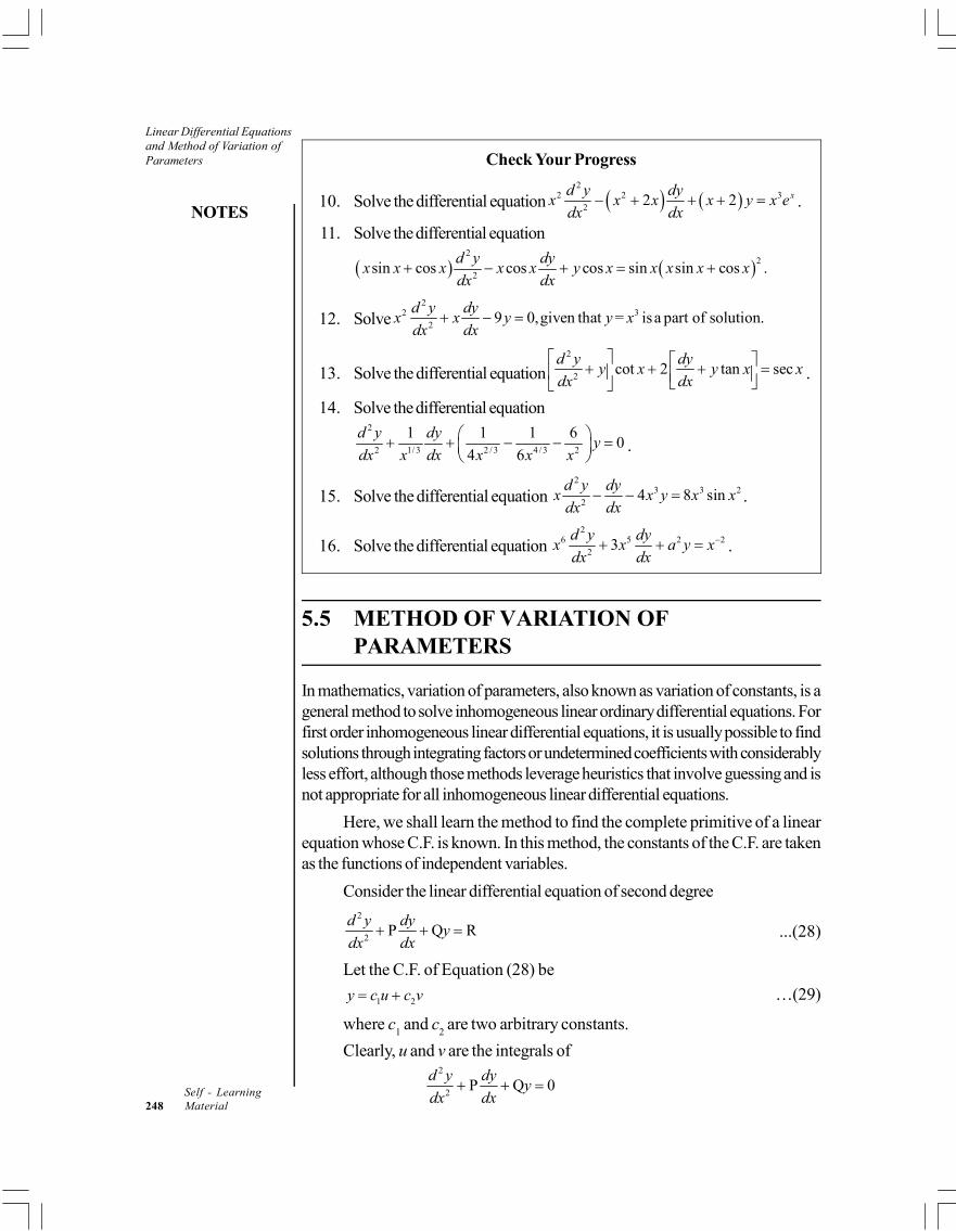
Linear Differential Equationsand Method of Variation ofParameters
NOTES
Self - Learning248 Material
Check Your Progress
10. Solve the differential equation 2
2 2 32
2 2 xd y dyx x x x y x e
dx dx .
11. Solve the differential equation
2
2
2sin cos cos cos sin sin cos .
d y dyx x x x x y x x x x x
dx dx
12. Solve2
2 32
9 0,given that = isa part of solution.d y dy
x x y y xdx dx
13. Solve the differential equation2
2cot 2 tan sec
d y dyy x y x x
dx dx
.
14. Solve the differential equation2
2 1/ 3 / 3 4 / 3 2
1 1 1 60
4 6
d y dyy
dx x dx x x x
.
15. Solve the differential equation 2
3 3 22
4 8 sind y dy
x x y x xdx dx
.
16. Solve the differential equation 2
6 5 2 22
3d y dy
x x a y xdx dx
.
5.5 METHOD OF VARIATION OFPARAMETERS
In mathematics, variation of parameters, also known as variation of constants, is ageneral method to solve inhomogeneous linear ordinary differential equations. Forfirst order inhomogeneous linear differential equations, it is usually possible to findsolutions through integrating factors or undetermined coefficients with considerablyless effort, although those methods leverage heuristics that involve guessing and isnot appropriate for all inhomogeneous linear differential equations.
Here, we shall learn the method to find the complete primitive of a linearequation whose C.F. is known. In this method, the constants of the C.F. are takenas the functions of independent variables.
Consider the linear differential equation of second degree2
2P Q R
d y dyy
dx dx ...(28)
Let the C.F. of Equation (28) be
1 2y c u c v …(29)
where c1 and c
2 are two arbitrary constants.
Clearly, u and v are the integrals of2
2P Q 0
d y dyy
dx dx
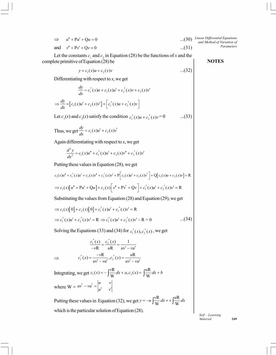
NOTES
Linear Differential Equationsand Method of Variation of
Parameters
Self - LearningMaterial 249
P Q 0u u u ...(30)
and P Q 0v v v ...(31)
Let the constants c1 and c
2 in Equation (28) be the functions of x and the
complete primitive of Equation (28) be
1 2( ) ( )y c x u c x v ...(32)
Differentiating with respect to x, we get
1 1 2 2( ) ( ) ( ) ( )dy
c x u c x u c x v c x vdx
1 2 1 2( ) ( ) ( ) ( )dy
c x u c x v c x u c x vdx
Let c1(x) and c
2(x) satisfy the condition
1 2( ) ( )c x u c x v = 0 ...(33)
Thus, we get 1 2( ) ( )dy
c x u c x vdx
Again differentiating with respect to x, we get2
1 1 2 22( ) ( ) ( ) ( )
d yc x u c x u c x v c x v
dx
Putting these values in Equation (28), we get
1 1 2 2 1 2 1 2( ) ( ) ( ) ( ) P ( ) ( ) Q ( ) ( ) Rc x u c x u c x v c x v c x u c x v c x u c x v
1 2 1 2( ) P Q ( ) P Q ( ) ( ) Rc x u u u c x v v v c x u c x v
Substituting the values from Equation (28) and Equation (29), we get
1 2 1 2( ) 0 ( ) 0 ( ) ( ) Rc x c x c x u c x v
1 2( ) ( ) Rc x u c x v 1 2( ) ( ) R = 0c x u c x v ...(34)
Solving the Equations (33) and (34) for 1 2( ), ( )c x c x , we get
1 2( ) ( ) 1
R R
c x c x
v u uv vu
1 2
R R( ) , ( )
v uc x c x
uv vu uv vu
Integrating, we get 1 2
R R( ) , ( )
W W
v uc x dx a c x dx b
where W = u v
uv vuu v
Putting these values in Equation (32), we getR R
W W
v uy u dx v dx
which is the particular solution of Equation (28).
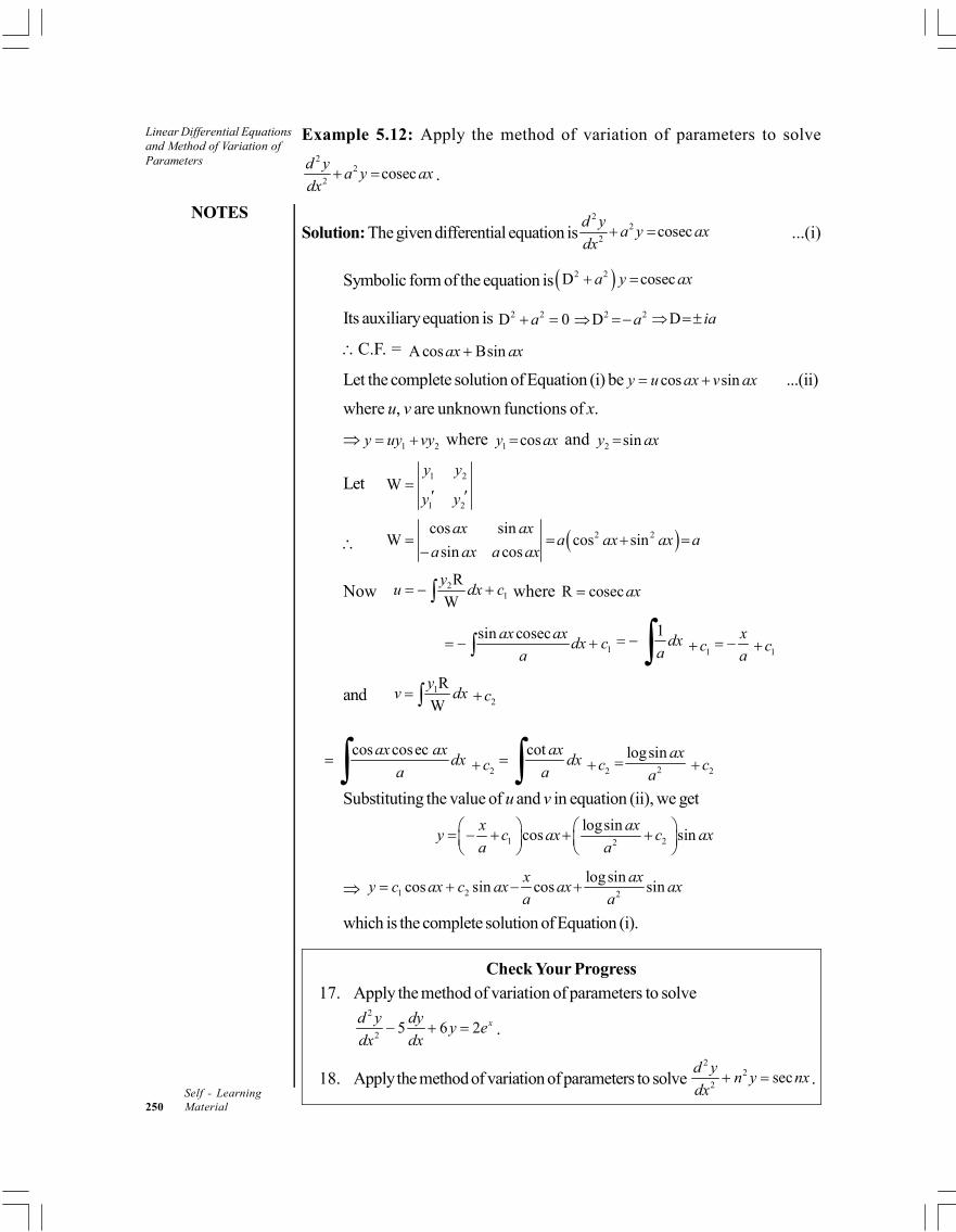
Linear Differential Equationsand Method of Variation ofParameters
NOTES
Self - Learning250 Material
Example 5.12: Apply the method of variation of parameters to solve2
22
cosecd y
a y axdx
.
Solution: The given differential equation is2
22
cosecd y
a y axdx
...(i)
Symbolic form of the equation is 2 2D coseca y ax
Its auxiliary equation is 2 2D 0a 2 2D a D ia
C.F. = A cos Bsinax ax
Let the complete solution of Equation (i) be cos siny u ax v ax ...(ii)
where u, v are unknown functions of x.
1 2y uy vy where 1 cosy ax and 2 siny ax
Let1 2
1 2
Wy y
y y
2 2cos sinW cos sin
sin cos
ax axa ax ax a
a ax a ax
Now 21
R
W
yu dx c where R cosecax
1
sin cosecax axdx c
a
1dx
a 1c
x
a
1c
and 1R
W
yv dx 2c
cos cosec ax ax
dxa
2ccot ax
dxa
2c 2
logsin ax
a
2c
Substituting the value of u and v in equation (ii), we get
1 22
logsincos sin
x axy c ax c ax
a a
1 2 2
logsincos sin cos sin
x axy c ax c ax ax ax
a a
which is the complete solution of Equation (i).
Check Your Progress
17. Apply the method of variation of parameters to solve2
25 6 2 xd y dy
y edx dx
.
18. Apply the method of variation of parameters to solve 2
22
secd y
n y nxdx
.
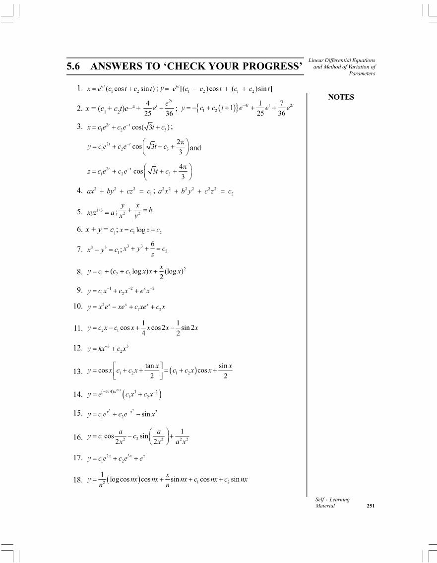
NOTES
Linear Differential Equationsand Method of Variation of
Parameters
Self - LearningMaterial 251
5.6 ANSWERS TO ‘CHECK YOUR PROGRESS’
1. 61 2( cos sin )tx e c t c t ; y 6
1 2 1 2[( )cos ( )sin ]te c c t c c t
2. x = (c1 + c
2t)e4 +
24
25 36
tt e
e ; 4 21 2
1 71
25 36t t ty c c t e e e
3. 21 2 3cos( 3 )t tx c e c e t c ;
21 2 3
2cos 3
3t ty c e c e t c
and
21 2 3cos 3
3t tz c e c e t c
4. 2 2 21ax by cz c ; 2 2 2 2 2 2
2a x b y c z c
5. 1/ 3xyz a ; 2 2
y xb
x y
6. x + y = c1; 1 2logx c z c
7. 3 31x y c ; 3 3
2
6x y c
z
8. 21 2 3( log ) (log )
2
xy c c c x x x
9. 1 2 21 2
xy c x c x e x
10. 21 2
x x xy x e xe c xe c x
11. 2 1
1 1cos cos 2 sin 2
4 2y c x c x x x x
12. 3 32y kx c x
13. 1 2 1 2
tan sincos cos
2 2
x xy x c c x c c x x
14. 2/ 33/ 4 3 21 2
xy e c x c x
15. 2 2 21 2 sinx xy c e c e x
16. 1 22 2 2 2
1cos sin
2 2
a ay c c
x x a x
17. 2 31 2
x x xy c e c e e
18. 1 22
1logcos cos sin cos sin
xy nx nx nx c nx c nx
n n
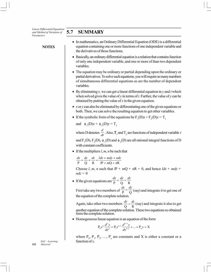
Linear Differential Equationsand Method of Variation ofParameters
NOTES
Self - Learning252 Material
5.7 SUMMARY
In mathematics, an Ordinary Differential Equation (ODE) is a differentialequation containing one or more functions of one independent variable andthe derivatives of those functions.
Basically, an ordinary differential equation is a relation that contains functionof only one independent variable, and one or more of than two dependentvariables.
The equation may be ordinary or partial depending upon the ordinary orpartial derivatives. To solve such equations, you will require as many numbersof simultaneous differential equations as are the number of dependentvariables.
By eliminating x, we can get a linear differential equation in y and t whichwhen solved gives the value of y in terms of t. Further, the value of y can beobtained by putting the value of x in the given equation.
x or y can also be eliminated by differentiating one of the given equations orboth. Then, we can solve the resulting equation to get other variables.
If the symbolic form of the equations be F1(D)x + F
2(D)y = T
1
and 1(D)x +
2(D)y = T
2
where D denotes d
dt. Also, TT
1 and T
2 are functions of independent variable t
and F1(D), F
2(D),
1(D) and
2(D) are all rational integral functions of D
with constant coefficients.
If the multipliers l, m, n be such that
P Q R P Q R
dy ldx mdy ndzdx dz
l m n
Choose l, m, n such that lP + mQ + nR = 0, and hence ldx + mdy +ndz = 0
If the given equations are P Q R
dydx dz
First take any two members of P Q
dydx (say) and integrate it to get one of
the equation of the complete solution.
Again, take other two members Q R
dy dz (say) and integrate it also to get
another equation of the complete solution. These two equations so obtainedform the complete solution.
Homogeneous linear equation is an equation of the form1
10 1 1
P P ... P Xn n
n nnn n
d y d yx x y
dx dx
where P0, P
1, P
2, …, P
n are constants and X is either a constant or a
function of x.
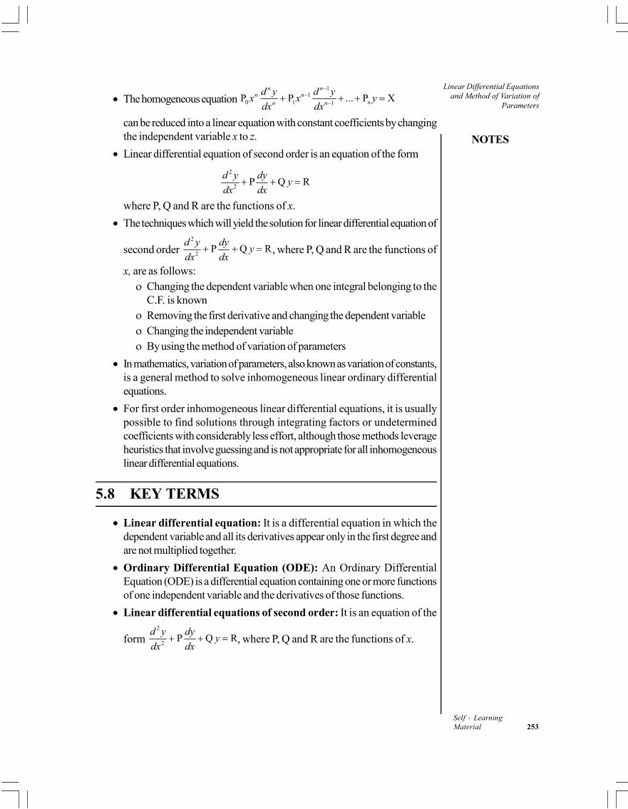
NOTES
Linear Differential Equationsand Method of Variation of
Parameters
Self - LearningMaterial 253
The homogeneous equation 1
10 1 1
P P ... P Xn n
n nnn n
d y d yx x y
dx dx
can be reduced into a linear equation with constant coefficients by changingthe independent variable x to z.
Linear differential equation of second order is an equation of the form
2
2P Q R
d y dyy
dx dx
where P, Q and R are the functions of x.
The techniques which will yield the solution for linear differential equation of
second order 2
2P Q R
d y dyy
dx dx , where P, Q and R are the functions of
x, are as follows: Changing the dependent variable when one integral belonging to the
C.F. is known Removing the first derivative and changing the dependent variable Changing the independent variable By using the method of variation of parameters
In mathematics, variation of parameters, also known as variation of constants,is a general method to solve inhomogeneous linear ordinary differentialequations.
For first order inhomogeneous linear differential equations, it is usuallypossible to find solutions through integrating factors or undeterminedcoefficients with considerably less effort, although those methods leverageheuristics that involve guessing and is not appropriate for all inhomogeneouslinear differential equations.
5.8 KEY TERMS
Linear differential equation: It is a differential equation in which thedependent variable and all its derivatives appear only in the first degree andare not multiplied together.
Ordinary Differential Equation (ODE): An Ordinary DifferentialEquation (ODE) is a differential equation containing one or more functionsof one independent variable and the derivatives of those functions.
Linear differential equations of second order: It is an equation of the
form 2
2P Q R
d y dyy
dx dx , where P, Q and R are the functions of x.
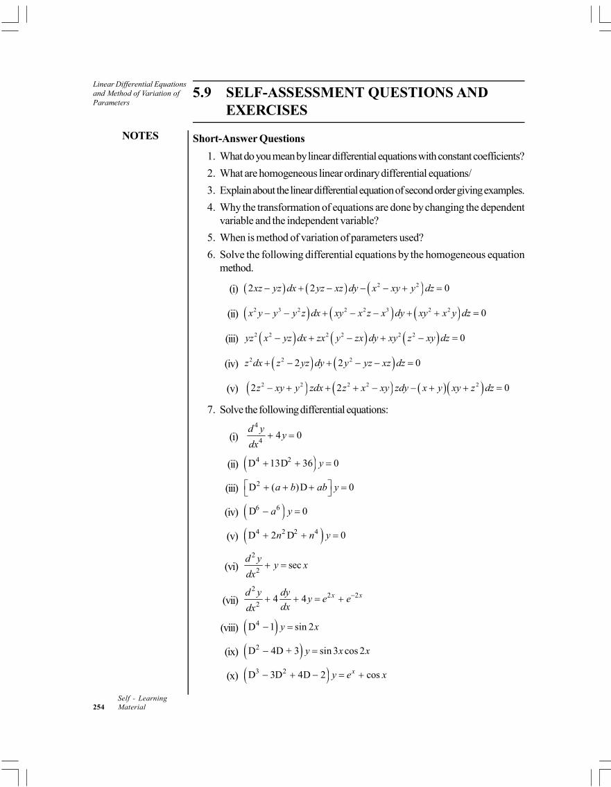
Linear Differential Equationsand Method of Variation ofParameters
NOTES
Self - Learning254 Material
5.9 SELF-ASSESSMENT QUESTIONS ANDEXERCISES
Short-Answer Questions
1. What do you mean by linear differential equations with constant coefficients?
2. What are homogeneous linear ordinary differential equations/
3. Explain about the linear differential equation of second order giving examples.
4. Why the transformation of equations are done by changing the dependentvariable and the independent variable?
5. When is method of variation of parameters used?
6. Solve the following differential equations by the homogeneous equationmethod.
(i) 2 22 2 0xz yz dx yz xz dy x xy y dz
(ii) 2 3 2 2 2 3 2 2 0x y y y z dx xy x z x dy xy x y dz
(iii) 2 2 2 2 2 2 0yz x yz dx zx y zx dy xy z xy dz
(iv) 2 2 22 2 0z dx z yz dy y yz xz dz
(v) 2 2 2 2 22 2 0z xy y zdx z x xy zdy x y xy z dz
7. Solve the following differential equations:
(i) 4
44 0
d yy
dx
(ii) 4 2D 13D 36 0y
(iii) 2D ( )D 0a b ab y
(iv) 6 6D 0a y
(v) 4 2 2 4D 2 D 0n n y
(vi)2
2sec
d yy x
dx
(vii)2
2 22
4 4 x xd y dyy e e
dxdx
(viii) 4D 1 sin 2y x
(ix) 2D 4D + 3 sin 3 cos 2y x x
(x) 3 2D 3D 4D 2 cosxy e x
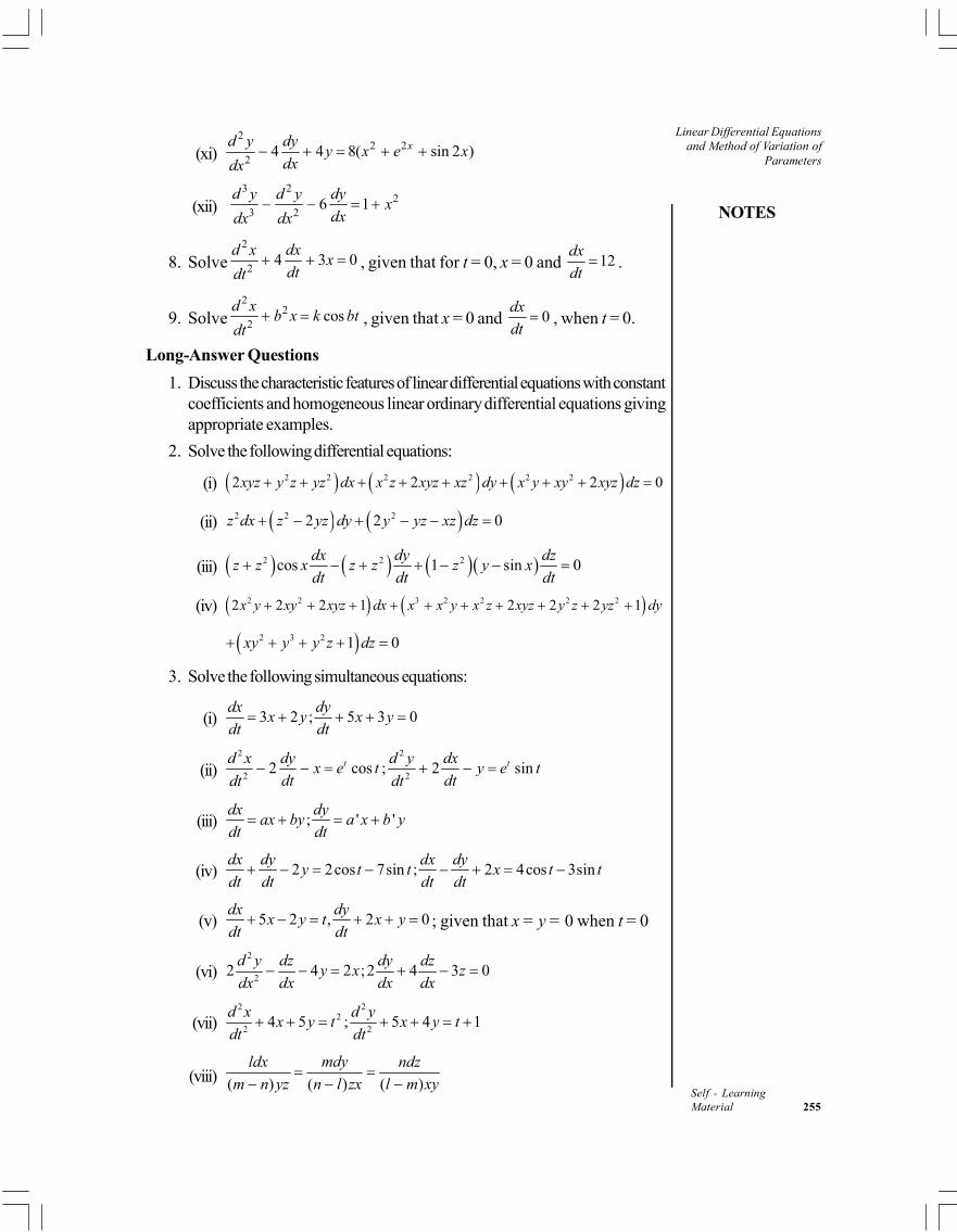
NOTES
Linear Differential Equationsand Method of Variation of
Parameters
Self - LearningMaterial 255
(xi)2
2 22
4 4 8( sin 2 )xd y dyy x e x
dxdx
(xii) 3 2
23 2
6 1d y d y dy
xdxdx dx
8. Solve2
24 3 0
d x dxx
dtdt , given that for t = 0, x = 0 and 12
dx
dt .
9. Solve2
22
cosd x
b x k btdt
, given that x = 0 and 0dx
dt , when t = 0.
Long-Answer Questions
1. Discuss the characteristic features of linear differential equations with constantcoefficients and homogeneous linear ordinary differential equations givingappropriate examples.
2. Solve the following differential equations:
(i) 2 2 2 2 2 22 2 2 0xyz y z yz dx x z xyz xz dy x y xy xyz dz
(ii) 2 2 22 2 0z dx z yz dy y yz xz dz
(iii) 2 2 2cos 1 sin 0dx dy dz
z z x z z z y xdt dt dt
(iv) 2 2 3 2 2 2 22 2 2 1 2 2 2 1x y xy xyz dx x x y x z xyz y z yz dy
2 3 2 1 0xy y y z dz
3. Solve the following simultaneous equations:
(i) 3 2 ; 5 3 0dx dy
x y x ydt dt
(ii)22
2 22 cos ; 2 sint tdy d yd x dx
x e t y e tdt dtdt dt
(iii) ; ' 'dx dy
ax by a x b ydt dt
(iv) 2 2cos 7sin ; 2 4cos 3sindx dy dx dy
y t t x t tdt dt dt dt
(v) 5 2 , 2 0dx dy
x y t x ydt dt
; given that x = y = 0 when t = 0
(vi)2
22 4 2 ;2 4 3 0
d y dz dy dzy x z
dx dx dx dx
(vii)2 2
22 2
4 5 ; 5 4 1d x d y
x y t x y tdt dt
(viii) ( ) ( ) ( )
mdyldx ndz
m n yz n l zx l m xy
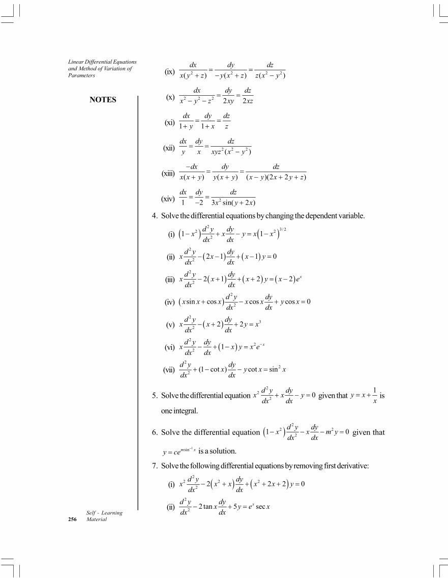
Linear Differential Equationsand Method of Variation ofParameters
NOTES
Self - Learning256 Material
(ix) 2 2 2 2( ) ( ) ( )
dx dy dz
x y z y x z z x y
(x) 2 2 2 2 2
dx dy dz
x y z xy xz
(xi) 1 1
dx dy dz
y x z
(xii) 2 2 2( )
dx dy dz
y x xyz x y
(xiii) ( ) ( ) ( )(2 2 )
dydx dz
x x y y x y x y x y z
(xiv) 21 2 3 sin( 2 )
dx dy dz
x y x
4. Solve the differential equations by changing the dependent variable.
(i) 2
3/ 22 22
1 1d y dy
x x y x xdx dx
(ii) 2
22 1 1 0
d y dyx x x y
dx dx
(iii) 2
22 1 2 2 xd y dy
x x x y x edx dx
(iv) 2
2sin cos cos cos 0
d y dyx x x x x y x
dx dx
(v) 2
32
2 2d y dy
x x y xdx dx
(vi) 2
22
1 xd y dyx x y x e
dx dx
(vii)2
22
(1 cot ) cot sind y dy
x y x xdx dx
5. Solve the differential equation 2
22
0d y dy
x x ydx dx
given that 1
y xx
is
one integral.
6. Solve the differential equation 2
2 22
1 0d y dy
x x m ydx dx
given that
1sinm xy ce
is a solution.
7. Solve the following differential equations by removing first derivative:
(i) 2
2 2 22
2 2 2 0d y dy
x x x x x ydx dx
(ii)2
22 tan 5 secxd y dy
x y e xdx dx
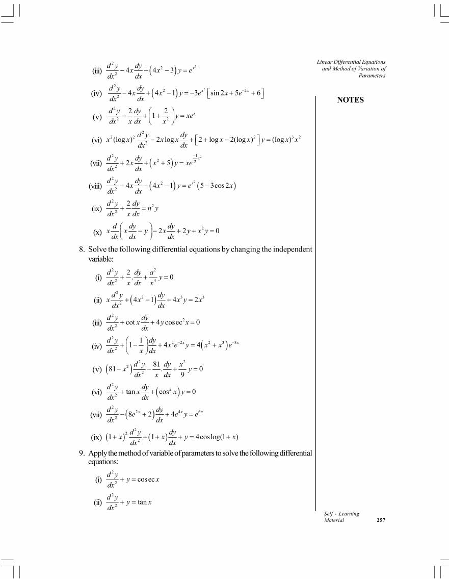
NOTES
Linear Differential Equationsand Method of Variation of
Parameters
Self - LearningMaterial 257
(iii) 22
22
4 4 3 xd y dyx x y e
dx dx
(iv) 22
2 22
4 4 1 3 sin 2 5 6x xd y dyx x y e x e
dx dx
(v) 2
2 2
2 21 xd y dy
y xedx x dx x
(vi)2
2 2 2 3 22
(log ) 2 log 2 log 2(log ) (log )d y dy
x x x x x x y x xdx dx
(vii) 212
2 22
2 5xd y dy
x x y xedx dx
(viii) 22
22
4 4 1 5 3cos2xd y dyx x y e x
dx dx
(ix)2
22
2d y dyn y
dx x dx
(x)22 2 0
d dy dyx x y x y x y
dx dx dx
8. Solve the following differential equations by changing the independentvariable:
(i)2 2
2 4
2. 0
d y dy ay
dx x dx x
(ii) 2
2 3 32
4 1 4 2d y dy
x x x y xdx dx
(iii)2
22
cot 4 cosec 0d y dy
x y xdx dx
(iv) 2
2 2 2 3 32
11 4 4x xd y dy
x e y x x edx x dx
(v) 2 2
22
8181 . 0
9
d y dy xx y
dx x dx
(vi) 2
22
tan cos 0d y dy
x x ydx dx
(vii) 2
2 4 62
8 2 4x x xd y dye e y e
dx dx
(ix) 2
2
21 1 4coslog(1 )
d y dyx x y x
dx dx
9. Apply the method of variable of parameters to solve the following differentialequations:
(i)2
2cosec
d yy x
dx
(ii)2
2tan
d yy x
dx
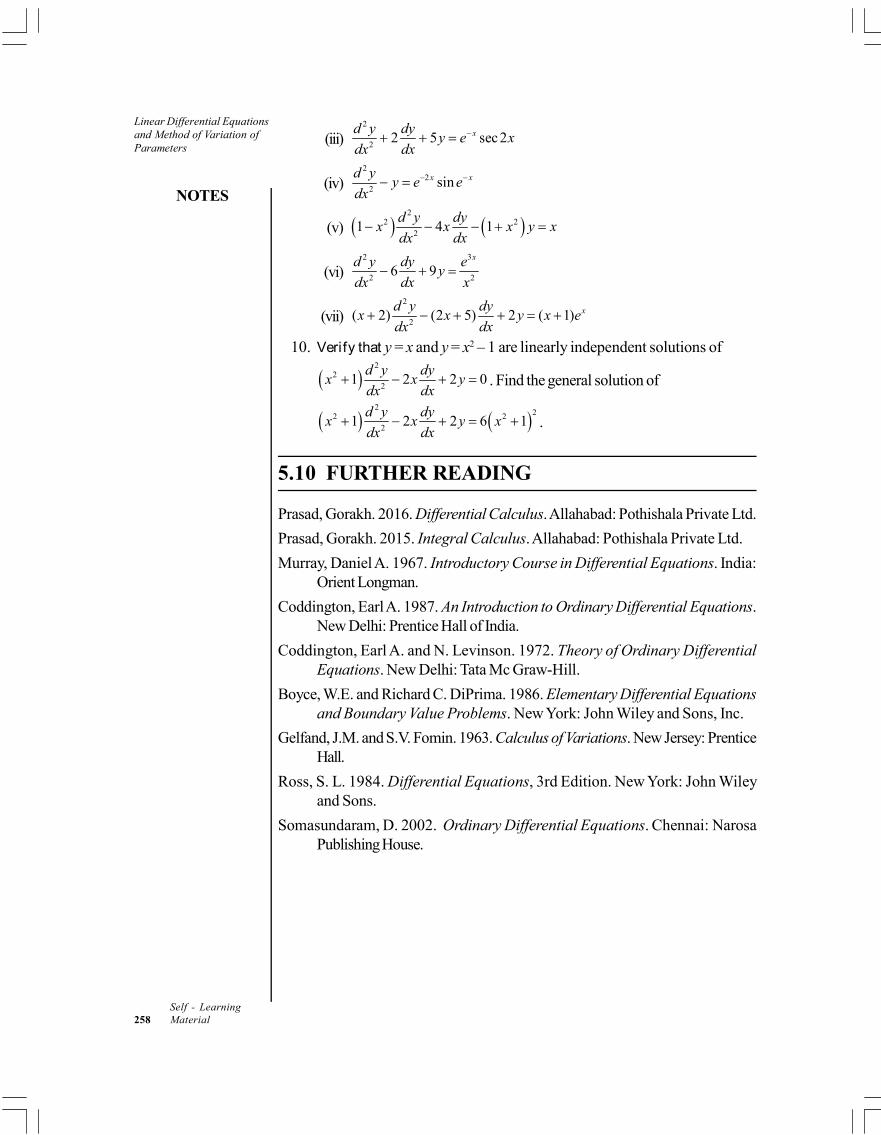
Linear Differential Equationsand Method of Variation ofParameters
NOTES
Self - Learning258 Material
(iii)2
22 5 sec 2xd y dy
y e xdx dx
(iv)2
22
sinx xd yy e e
dx
(v) 2
2 22
1 4 1d y dy
x x x y xdx dx
(vi)2 3
2 26 9
xd y dy ey
dx dx x
(vii)2
2( 2) (2 5) 2 ( 1) xd y dyx x y x e
dx dx
10. Verify that y = x and y = x2 – 1 are linearly independent solutions of
2
22
1 2 2 0d y dy
x x ydx dx
. Find the general solution of
2
22 22
1 2 2 6 1d y dy
x x y xdx dx
.
5.10 FURTHER READING
Prasad, Gorakh. 2016. Differential Calculus. Allahabad: Pothishala Private Ltd.
Prasad, Gorakh. 2015. Integral Calculus. Allahabad: Pothishala Private Ltd.
Murray, Daniel A. 1967. Introductory Course in Differential Equations. India:Orient Longman.
Coddington, Earl A. 1987. An Introduction to Ordinary Differential Equations.New Delhi: Prentice Hall of India.
Coddington, Earl A. and N. Levinson. 1972. Theory of Ordinary DifferentialEquations. New Delhi: Tata Mc Graw-Hill.
Boyce, W.E. and Richard C. DiPrima. 1986. Elementary Differential Equationsand Boundary Value Problems. New York: John Wiley and Sons, Inc.
Gelfand, J.M. and S.V. Fomin. 1963. Calculus of Variations. New Jersey: PrenticeHall.
Ross, S. L. 1984. Differential Equations, 3rd Edition. New York: John Wileyand Sons.
Somasundaram, D. 2002. Ordinary Differential Equations. Chennai: NarosaPublishing House.
Related Documents


