Caffeinated Development: Exports, Human Capital, and ...

Caffeinated Development: Exports, Human Capital,and Structural Transformation in Colombia∗

Mateo Uribe-Castro†

This version: January 21, 2021Latest version here

Abstract

This paper studies the effect of the first wave of globalization on developing countries’ structuraltransformation, using data from Colombia’s expansion of coffee cultivation. Counties engaged incoffee cultivation in the 1920s developed a smaller manufacturing sector by 1973 than comparablecounties, despite starting at a similar level in 1912. My empirical strategy exploits variation inpotential coffee yields, and variations in the probability to grow coffee at different altitudes. Thispaper argues that coffee cultivation increased the opportunity cost of education, which reducedthe supply of skilled workers, and slowed down structural transformation. Using exogenous ex-posure to coffee price shocks as instrument, I show that reductions in cohorts’ educational attain-ment led to lower manufacturing activity in the long-run. The effect is driven by both a decreasein demand for education and reductions in public goods. Finally, coffee cultivation during theearly 20th Century had negative long-run effects on both individual incomes and poverty rates.JEL: O14, N16, N56, N66.

Keywords: structural transformation, human capital, exports, coffee.

∗I am grateful to John Wallis, Ethan Kaplan, and Allan Drazen for continued advice and support. I also want to thank Francesco

Bogliacino, Maria M. Botero, Ryan Edwards, Irina Espana, Martin Fiszbein, Jessica Goldberg, Javier Mejia, Jacopo Ponticelli, Santiago

Perez, Pablo Querubin, Michele Rosenberg, Felipe Saffie, Fernando Saltiel, Lesley Turner, Cody Tuttle, Sergio Urzua, Felipe Valencia, Daniel

Velasquez, and participants at Cliometric Society, EHA Meetings, NBER SI-DAE, NEUDC, RIDGE Economic History, U. Nacional Colombia,

LACEA, UMD Applied Micro, and UMD Political Economy workshop for their feedback and comments. Santiago Uribe and Pedro Uribe

provided invaluable help with the data collection process.†Department of Economics, Universidad del Rosario; Email: [email protected]

1

1 Introduction

The first wave of globalization at the dawn of the 20th century allowed countries that had

not yet industrialized to expand their agricultural production to supply world demand

(O’Rourke and Williamson, 2002). Were these export opportunities leveraged for expand-

ing the industrial sector? Or, on the contrary, did those places focus on agriculture and

delay industrialization? Whether the rise in agricultural exports helped the development

of manufacturing and services -the process of structural transformation- is a central ques-

tion on development economics and has been debated for decades (Rosenstein-Rodan,

1943; Lewis, 1955; Schultz, 1964; Kuznets, 1966). In general, theoretical contributions high-

light potential mechanisms in both directions.1 The debate has influenced political views

about globalization as well as trade and industrial policy in developing countries since the

post-war period (Cardoso and Faletto, 1979; Wallerstein, 2011). But the direction of the

change in structural transformation resulting from the expansion of agricultural exports

is context-specific and, ultimately, an empirical question.

This paper provides new evidence on the effect of the first wave of globalization on

developing countries’ processes of structural transformation on the long run. Specifically,

I study the effect of Colombia’s expansion of coffee cultivation on industrialization and

economic development.2 A long peaceful period after 1902 and the construction of the

Panama Canal in 1914 allowed the country to increase its participation in global trade by

introducing a new labor-intensive crop, coffee, to areas mostly used to produce maize,

beans, and other staples for local consumption (Parsons, 1949). Colombia’s broken geog-

raphy generated a set of local economies relatively isolated from one another and com-

parable in terms of size and population. Rich variation in climatic conditions within the1The direction may depend on the degree of trade openness (Matsuyama, 1992), income elasticity of

demand for manufacturing goods (Murphy et al., 1989), changes on terms of trade (Prebisch, 1950), depthof linkages with the rest of the economy (Hirschman, 1958), or features of crops’ production function (En-german and Sokoloff, 1997; Vollrath, 2011).

2The four-fold coffee production expansion between 1905 and 1921 is comparable to the largest expansionof modern agricultural exports (Palm oil in Indonesia (Edwards, 2019)).

2

country provides a good setting to study how the opportunity to produce an agricultural

export good impacted long-run development.

This paper shows the expansion of coffee cultivation deterred industrialization. Coun-

ties producing coffee beans around 1920 developed a weaker manufacturing sector through

the 20th century. Though manufacturing employment was consistent among coffee-bean-

cultivating counties and non-coffee-bean-cultivating counties in 1912, the expansion of

agricultural exports had a negative and sizable effect on manufacturing employment in

1938, 1973, and 2005, reaching its peak in 1973. By 2005, coffee cultivation’s effect on man-

ufacturing employment had halved, which follows the pattern of Colombia’s structural

transformation established in Figure 1. Consequently, I show that counties producing cof-

fee beans around 1920 had lower population density and higher poverty rates as of 2005.

Identifying the causal relationship between coffee cultivation and structural transfor-

mation is challenging. Counties that would not have developed a strong manufacturing

sector through the 20th century could have taken up coffee cultivation as an alternative.

For instance, regions that had more difficulty importing capital goods might have seen

a profitable opportunity in coffee bean production since it was transportable by mules.

What would appear to be a negative effect of coffee bean cultivation on industrialization,

could, in fact, be driven by geography or location.

In this paper, I exploit two different sources of variation related to climatic conditions

to address endogeneity concerns. The assumption behind both instruments is that climatic

conditions specific to coffee trees only affect industrialization through coffee cultivation.

The first instrument for 1920 coffee cultivation is the average potential coffee yield from

FAO’s Global Agro-Ecological Zones project. FAO-GAEZ estimates potential coffee bean

yields at a high-resolution level using a combination of local climatic conditions and cof-

fee’s growth cycle. The second instrument exploits a discontinuous reduction in the prob-

ability that a county grew coffee trees at 2,400 meters above sea level (7,874ft). The dis-

continuity is explained by both low temperatures in counties above the altitude threshold

3

and the dissemination of information regarding coffee cultivation in the late 19th century.

Optimal temperatures to grow coffee trees ranged between 16 and 24 degrees Celsius (60

to 75 degrees Farenheit). Given Colombia’s tropical location, the temperature bandwidth

mapped directly to an altitude bandwidth between 400 and 2,400 meters. Moreover, 19th

century pamphlets promoting coffee cultivation explicitly identified towns just below and

just above the upper altitude threshold as a reference due to lack of easily available ther-

mometers3 (Saenz, 1892). This fuzzy regression discontinuity strategy compares counties

with average altitudes higher and lower than 2,400 meters. The main specification restricts

the sample to include counties above 1,800 meters to guarantee an equal number on each

side of the threshold.

The expansion of coffee cultivation in Colombia was effectively a land-augmenting

technical change. A simple two-sector model with land-augmenting productivity can ex-

plain employment reallocation from manufacturing into agriculture, as Bustos et al. (2016)

show using data from Brazil after 1990. However, a theory that explains coffee’s negative

effect on manufacturing employment must also account for the fact that around 80% of

Colombia’s labor force was employed in agriculture in 1912. It must explain the differen-

tial evolution of industrialization between coffee and non-coffee counties. Such a theory

would apply more generally to developing countries during the first wave of globalization,

before the proliferation of industrialization.

Using historical and present-day data at the local level, the empirical specifications

compare structural transformation patterns throughout the 20th century between places

that did and did not produce coffee beans around 1920. This approach is relevant for

two reasons: first, Colombian counties during the early 20th century are characterized

by low labor mobility and connected product markets. Since they behave as small open

economies, empirical evidence from local units can be tied to insights from theoretical

models (e.g. Foster and Rosenzweig (2004), Bustos et al. (2016) and Fiszbein (2017)). Sec-3As illustrated in Figure 6.

4

ond, it highlights the distributional consequences of trade across local economies within

countries. Though these consequences are well documented for late 20th century global-

ization (Autor et al., 2016; Goldberg and Pavcnik, 2007), evidence is scarce for the early

20th century. If the effect of trade on structural transformation depends on an economy’s

stage of development, evidence from more recent periods might not be as informative.

Given coffee’s labor-intensive production function, the expansion of coffee cultivation

increased the opportunity cost of education. Therefore, the supply of skilled workers in

coffee-cultivating counties increased at a slower pace relative to other counties, which in

turn slowed growth in the manufacturing sector. The argument connecting human capital

and structural transformation is formalized explicitly by Caselli and Coleman II (2001)

and indirectly by Acemoglu and Guerrieri (2008). Porzio and Santangelo (2019) use data

across countries and within districts in Indonesia to provide causal evidence of the positive

role of schooling in industrialization through increases in availability of workers for non-

agricultural sector. This paper adds to the empirical evidence on supply-side mechanisms,

specially related to education, as mediators in the process of industrialization.

Two pieces of evidence support the human capital mechanism. First, the difference

in manufacturing employment between coffee and non-coffee counties is concentrated

in sectors intensive in human capital, classified according to Ciccone and Papaioannou

(2009). Second, I present difference-in-differences evidence from comparing adults in the

1973 census of population born between 1902 and 1952. Different cohorts were exposed

to different world coffee prices while they were of school age, which determined the op-

portunity cost of dropping out of school. Cohorts born in coffee counties and exposed to

higher coffee prices during school age accumulate fewer years of education by 1973.

These results contribute to a growing empirical literature on how export booms re-

duce human capital accumulation (e.g. Bobonis and Morrow (2014); Atkin (2016); Svi-

atschi (2018)). Moreover, they complement Carrillo (2019), who finds a negative, though

smaller, effect of coffee price shocks on education using data from the second half of the

5

20th century4 This paper looks at coffee price shocks during the first half of the century,

when industrialization first spread, and focuses on coffee cultivation’s effect on structural

transformation.

The fact that coffee cultivation leads to lower levels of education could be a conse-

quence of both household decisions and changes in supply of schooling. For instance,

landowners in coffee regions might oppose the construction of schools or limit funding

to existing ones in order to guarantee supply of agricultural workers (Galor et al., 2009;

Galiani et al., 2008). I leverage data on county level land inequality between coffee farms

to provide suggestive evidence of both education supply and demand channels. In other

words, coffee-bean-producing counties develop a less skilled labor force due to individ-

ual’s decisions to drop out of school and a lower number of schools per capita by 1951.

Coffee price shocks also had a negative direct effect on employment in manufacturing

in 1973. The share of the labor force employed in manufacturing in 1973 is lower for cohorts

born in coffee counties who were exposed to higher coffee prices during school age. The

effect is similar in magnitude to the effect on education. Mediation analysis Dippel et al.

(2019b) suggests around 70% of the effect of 1920 coffee cultivation on 1973 manufacturing

employment is mediated by the effect of coffee cultivation on education. This result is

only suggestive of the importance of the effect because it relies on one strong assumption:

the sources of omitted variable bias present when estimating coffee’s effect on cohort’s

education are identical to the ones that would bias the estimation coffee’s effect on cohort’s

employment in manufacturing.

Finally, this paper explores other potential mechanism cited in the Colombian eco-

nomic history literature: linkages between coffee cultivation and manufacturing (e.g. Ocampo

(1984)). I exploit variation within coffee-bean-producing counties in terms of linkages

with non-agricultural sectors by exploring one crucial stage in coffee bean exports: thresh-4The effect I present in this paper is almost twice as large as Carrillo (2019) findings. The difference might

be due to reduction in transportation costs, changes in education’s rate of return or better enforcement ofchild labor and mandatory elementary school laws between the first and second half of the century.

6

ing, or removing the husk from the coffee bean. Threshing machines needed reliable en-

ergy sources that were also useful for manufacturing activities. Since they were imported

from Britain, the presence of threshing machines also signals connection with interna-

tional trade. Threshing also benefited smelting businesses that provided parts to con-

stantly repair them. I find, however, that the effect of 1920 coffee cultivation on manu-

facturing employment in 1973 does not depend on the presence of threshing machines.

Stronger linkages do not prevent coffee cultivation from having a negative effect on struc-

tural transformation.

This paper contributes to the empirical literature on the effect of agriculture on struc-

tural transformation and local development through productivity increases (Foster and

Rosenzweig, 2004; Hornbeck and Keskin, 2015; Moscona, 2018; Bustos et al., 2016) or other

factors (Fiszbein, 2017; Droller and Fiszbein, 2019). By highlighting human capital as a rel-

evant mechanism, my findings relate to studies looking at differences in living standards

at the subnational level that result from productivity gaps between agricultural and non-

agricultural employment (Acemoglu and Dell, 2010; Gennaioli et al., 2013; Gollin et al.,

2014; Herrendorf and Schoellman, 2018).

This paper’s argument about the role of human capital on the onset of industrializa-

tion in developing countries complements scholarship about Europe’s Industrial Revolu-

tion (Galor and Moav, 2004; Squicciarini and Voigtlander, 2015; Franck and Galor, 2017;

de la Croix et al., 2018). Similarly, this paper fits in with recent works on Latin American

economic history which highlight the role of human capital in the process of structural

transformation either directly (Valencia Caicedo, 2019) or indirectly (Perez, 2017). This

paper adds to the study of the adoption of coffee cultivation in Colombian history. As

(McGreevey, 1971, p. 198) put it: “No other substantive economic change in Colombian

economic history can have been of such overriding social importance.” This paper brings

comprehensive data and modern econometrics to an old debate in Colombian economic

history. It revisits an established literature studying the relationship between coffee cul-

7

tivation and industrialization that mostly rely on comparative studies or time series data.

The next section describes this literature in more detail.

Afterwards, I turn to the empirical analysis. Section 3 describes the main datasets used

in later sections. Section 4 presents main correlations between coffee cultivation and struc-

tural transformation. It also discusses the main obstacles for identification and presents

the empirical strategies used in Section 5. Sections 6 and 7 discuss potential mechanisms.

Finally, 8 discusses the long term effects of coffee cultivation on income and urbanization.

2 Exports and Structural Transformation in Colombia

Countries in Latin America started their processes of industrialization around the first

two decades of the 20th century. There was considerable heterogeneity in the path and

timing of structural transformation across the region (Salvucci, 2006; Duran et al., 2017).

While some countries like Argentina or Mexico had developed manufacturing industry by

1900, smaller countries struggled to consolidate industrial activities (Williamson, 2011).

Development economists and economic historians have argued that differences in the fea-

tures of the export sector help to explain the diverse experiences with industrialization.

What Bulmer-Thomas (2003) called “the lottery of commodities” has explanatory power

to understand the development of manufacturing in the region.

Demand for commodities from the world economy might help develop the non-export

economy through increases in income that increase demand for locally produced manu-

facturing. This is more likely to happen if the export sector benefits a large fraction of the

population and if transportation costs for imported manufactured goods are high (Mur-

phy et al., 1989; Matsuyama, 1992). Additionally, different export products had differ-

ent degrees of connection with other economic activities. Linkages or complementarities

of exports are cited as a reason for successful development of manufacturing (Bulmer-

Thomas, 2003; Hirschman, 1958).

8

These conditions were not met, for instance, for crops like bananas, produced in en-

claves with limited population, or for mining activities performed in isolation from the

main centers of population Bulmer-Thomas (2003). On the contrary, successful episodes

of industrial growth, like Argentina around 1900, have traditionally been explained by

the presence of agricultural activities like wheat or the exporting of processed meat that

were not available in other countries in the region. Recent empirical evidence by Droller

and Fiszbein (2019) support the hypothesis that linkages in agricultural activities generate

industrial growth.

Colombia did not consolidate its export sector until coffee cultivation took off around

1910. During the 19th century gold was consistently the main export, with a couple of

short experiments with tobacco and quinine (Ocampo, 1984). Even though coffee was

relatively new in the country, a long period of peace after 1902 and two coffee price booms

(1906 and in the 1920s) allowed coffee to grow until it represented more than 80% of ex-

ports by 1940 (Nieto Arteta, 1971). Coincidentally, manufacturing took off around the

1930s. It had been relegated to cottage industry during the first two decades of the cen-

tury, but more modern establishments appeared during the 30s and 40s (Ocampo and

Montenegro, 2007).

Historians and economic historians have interpreted this coincidence in timing as ev-

idence of the causal positive effect of coffee cultivation on the development of manufac-

turing, though the claim has been subject to extensive debate.5 Some features of coffee

cultivation fit the two theories explained above. Coffee directly employed 18% of the labor

force at its peak (McGreevey, 1971). Moreover, its production and exporting connected5Some version of this claim is discussed in the main economic history textbooks. The argument starts

with Ospina Vasquez (1955) and Parsons (1949). McGreevey summarizes the argument saying: “the rapidgrowth of a new export product raised income levels and generated new demands for imported and locallyproduced goods of all kinds” (McGreevey, 1971, p.198). Brew (1973), Nieto Arteta (1971) and Palacios(2002) studied coffee cultivation and its social impacts to Colombia’s and Antioquia’s societies. Arango(1981) focused exclusively on the direct connection between coffee and manufacturing. Bejarano (1980)summarizes the literature up to 1980 and Ocampo and Botero (2000), Ocampo (2015) discuss new develop-ments from the past 40 years. More modern literature on Colombia’s industrialization downplays the roleof coffee cultivation using network data on entrepreneurs and elite members (Mejia, 2018).

9

an extensive area and required machinery and manufacturing products like sacks.

Proponents of the positive link between coffee cultivation and manufacturing back

their claims with time series or Department level data. In this paper I collect a wealth

of historical data at both the county and individual level to empirically estimate the con-

nection between coffee cultivation and structural transformation.

2.1 Coffee in Colombia: Historical Background

Colombia went from producing around 230 thousand bags per year in 1900 to 3.2 million

in 1932. Figure 1a shows the evolution of exports during the first half of the 20th century.

At the end of the 19th century, the Eastern part of the country produced most of the coffee.

The crop made its way to Colombia’s West and South West in the first two decades of

the 20th century, well after the frontier closed (Parsons, 1949). By 1930, the East only

produced around 30% of total coffee exports.

Early adopters of the crop wrote several pamphlets around 1880 to inform potential

investors of the opportunities that coffee cultivation provided. Those pamphlets were col-

lected in the book Memorias sobre el cultivo del cafeto (Saenz, 1892). They provide infor-

mation about the different features of coffee’s production function at the turn of the 20th

century. In this paper, I highlight four of them.

First, producing coffee was labor intensive. Coffee trees had two large crops during the

year, but it was possible to collect coffee cherries all year round. Even when labor was not

required to pick the cherries, coffee farms demanded constant labor for other purposes

like weeding, pruning, and pest control. Second, the pamphlets highlighted that a lot of

the tasks involved in the collection and classification of coffee were ideal for children. I

argue in this paper that those two features of coffee production function shaped incentives

to accumulate human capital and ultimately affected coffee counties’ process of structural

transformation and development.

Third, the production of coffee required heavy machinery to remove the final grain for

10

exporting from its husk. This process known as threshing6 used imported machines, gen-

erally owned by farmers’ cooperatives. Not every coffee producing county had threshing

machines. They were in strategic locations, not necessarily in the main production centers.

In this paper, I argue coffee cultivation in counties with threshing machines had stronger

linkages to the non-export economy. I use this fact to test whether the effect of coffee cul-

tivation on manufacturing depended on linkages.

Finally, coffee was ideally produced at medium altitude. Those pamphlets consis-

tently pointed out that coffee could be produced between 24 and 16 degrees Celsius (76

to 60 Fahrenheit). Given that climate in Colombia is determined by altitude, early cof-

fee adopters provided reference points in terms of altitude to decide which terrains were

feasible to produce the crop. Figure 6 shows one of those instances. It highlights that

coffee could be produced near Rionegro, located at an altitude of 2,200 meters, but could

not be produced near Sonson or Santa Rosa, at altitudes of 2,500 and 2,450 meters respec-

tively. In general, authors of the pamphlets recognized there was an altitude bandwidth

inside which coffee cultivation was suitable. In this paper, I use the upper threshold of the

bandwidth in order to identify the causal effect of coffee cultivation on structural transfor-

mation.

3 Data

The empirical analysis in this paper spans several decades and uses information from var-

ious sources. Moreover, as this paper estimates the effect of exports on local development,

it is crucial to consistently define the unit of observation. Colombia’s population was dis-

tributed in 18 Departamentos during most of the 20th century. There were also a handful

of Intendencias, where population density was lower and most of the land was unsettled.

The country’s smallest political division are municipios, equivalent to US counties. They6In Spanish: trilla.

11

were generally comprised of a town (Cabecera) and a rural area. In this paper, I refer to

them as “counties.” They are the main unit of observation, as each one of them represents

a local economy.

I digitized county-level data from Colombia’s first coffee census (published in 1927)

and 1912 and 1938 census of population. Additionally, I use 1945 First Census of Manu-

facturing. I match 1927, 1938, and 1945 counties to the set of 741 counties reported in 1912

Census. Whenever I could not match by name, I used historical sources to match a county

created after 1912 to its “parent” 1912 county. This procedure yields a set of 734 counties

with observations in 1912, 1927, 1938, and 1945. Figure 7 shows population patterns in

1912 and highlights the main sample.

I also use 1973 and 2005 Census of Population, available from IPUMS International

(Ruggles et al., 2003). IPUMS homogenizes counties over time by merging small coun-

ties in terms of population and pooling them together into larger units. I call those units

“IPUMS-county”. There are 564 in 2005 Census. The average IPUMS-county contains 1.9

actual counties (municipios). However, 57% of IPUMS-counties only contain one actual

county. 84.4% of IPUMS-counties contain one or two actual counties. Moreover, out of

the 564 counties, only 495 counties can be traced to be part of a 1912 county. The other 69

counties are located in land that was colonized after 1950.

For each set of results, I explicitly define the unit of observation it uses, between coun-

ties and IPUMS-counties. I do this for two reasons: first, counties better represent local

economies for the first part of the 20th century. I use IPUMS-counties for results for the

second half of the 20th century, where larger units capture better the idea of a local econ-

omy. Second, even though there are some differences, there is significant overlap between

both definitions. Results using counties look qualitatively similar as those using IPUMS-

counties, but since the sample size is smaller, power tends to be lower.

12

Coffee cultivation before 1920

I measure coffee cultivation at the beginning of the 20th century with the number of coffee

trees used in production by county. This measure comes from the first coffee producers’

census: Monsalve’s 1927 book, “Colombia Cafetera.” Monsalve was an agricultural en-

gineer who led Colombia’s Propaganda and Information Office between 1920 and 1924.

During that period, he surveyed coffee farms around the country and put together a 950-

page book describing Colombia’s coffee industry. In 1924, Colombia’s government bought

the book’s rights. The goal was to promote coffee exports by “distributing the book to for-

eign markets, giving it out for free to public offices, and charging only the production cost

to private individuals.” Since coffee trees take around 5 years to start producing coffee

cherries, the number of coffee trees registered in Monsalve’s census is likely to represent

trees that were planted in the 1910s, even though the book was eventually published in

1927. Therefore, I interpret the number of coffee trees as a measure of early exposure to

coffee cultivation. For robustness, I also use the extensive margin, a dummy equal to one

for counties with a positive number of coffee trees planted before 1924.

The average county had 427 thousand coffee trees, equivalent to around 95 hectares,

but the distribution is skewed to the left. 43% of counties had no early coffee production.

50% of counties had less than 20,000 trees, which is equivalent to less than half a hectare.

These figures show how even though coffee was taking off during 1910s and 20s, it still

represented a small share of counties’ land. For instance, Fredonia (Antioquia) had the

largest number of coffee trees used for production in 1920. Its 8.3 million trees were equiv-

alent to 1,800 hectares or 7% its total area. As a comparison, using data from 2005 coffee

census, 22% of counties use more than 7% of their area to produce coffee. Chinchina (Cal-

das) was the county with highest concentration of coffee trees in 2005. It devoted 44% of

its area to the crop.

I use the coffee census to measure land inequality between coffee landowners. I cal-

culate the ratio between the average and the median farm for each county with a positive

13

number of coffee trees. This ratio was 1.9 for the average coffee county. Appendix A de-

scribes the calculation in more detail. A typical coffee county had around 85 coffee farms

and 5,600 inhabitants in 1912. A typical farm had 10 to 30 thousand trees. At a rate of23

pounds per tree per year, a typical coffee farm could produce between 110 and 330 60-

pound bags per year.

Economic structure

I measure population, population in the labor force, and shares of labor force employed

in manufacturing, agriculture, and services in 1912, 1938, 1973, and 2005. I digitized 1912

and 1938 Census of Population at the county level. I aggregated IPUMS International’s

Census samples (Ruggles et al., 2003) to build measures at the county level for 1973 and

2005. Additionally, I estimated shares of population who could read and write (1912, 1938,

1973, and 2005), average years of schooling of adult population by county (1973 and 2005),

and created household income measures using Filmer and Pritchett (2001) methodology

to summarize information about housing quality and durable goods (1973 and 2005).

1912 and 1938 Census of Population provide headcounts for different “Professions and

Occupations” at the county level. 1912 census counted the “Active Population” and di-

vided it between occupations.7 I consider Agriculture as the combination between Agri-

culture and Cattle Raising. Manufacturing sector is given by the “Crafts and Manufactur-

ing” category, while Services adds up Liberal Professions, Commerce, and Transportation.

1938 Census was also a series of headcounts at the county level, but the division between

occupations was more detailed. Occupations were divided between Primary Production,

Transformation Industries, Services, Liberal Activities, and Other. I define Agriculture

as Primary Production employment not in “Extractive Activities” such as mining. Man-

ufacturing employment is given by employment in Transformation Industries excluding71912 Occupations are: Liberal Professions, Arts, Crafts and Manufacturing, Priests and Nuns, Public

Employees, Military, Policemen, Agriculture, Cattle Raising, Commerce, Transportation, and Domestic Em-ployees.

14

“Construction and Buildings” Finally, Services is its own category formed by Transporta-

tion, Commerce, and Banking subdivisions.

I build measures of economic structure at the county level for 1973 and 2005 using in-

dividual level data from IPUMS International. To make it comparable with 1912 and 1938

figures, I calculate share of population in the labor force. Then I build counts of people

employed in Agriculture, Manufacturing, and Services to calculate shares of labor force

employed in each category. Additionally, I focus on population between 18 and 65 years

old to estimate household income measures. I follow Filmer and Pritchett (2001) and use

the first vector out of a Principal Component Analysis using information on housing qual-

ity (roof and floor materials, number of rooms, connection to electricity and sewage) as

well as durable goods consumption (washing machine, radio, refrigerator). Throughout

the calculations explained in this paragraph, I weight individuals according to their sam-

ple weight provided by IPUMS. Further details are explained in Appendix A.

A different measure of economic structure comes from Colombia’s First Manufactur-

ing Census in 1945. This Census measures more established type of manufacturing than

using data from employment out of Census of Population. Plants with five or more em-

ployees provided information about employment, wages, and financial status (Santos Car-

denas, 2017). The census contains information for 458 municipalities. It divides the es-

tablishments in 15 different sectors. Following Ciccone and Papaioannou (2009) and Va-

lencia Caicedo (2019), I classified the sectors in three groups according to their human

capital requirements (high, medium, low). I measure the share of population working in

industrial establishments with five or more employees, as well as shares of employment in

each of the three human capital groups. I interpolate 1938 and 1951 census of population

to obtain 1945 population data at the county level.

15

Human capital

The main measure of human capital comes from 1973 Census of Population. This is the

first available census with individual-level data that reports county of birth. I use this in-

formation to build a panel at the gender by cohort by county-of-birth level for individuals

born between 1900 and 1951. That is cohorts that are between 73 and 21 years old in 1973. I

measure cohorts’ average year of schooling, share of cohort-county-of birth who is literate,

and occupations shares of the labor force as well as labor force participation information

and average household income.

I combine 1973 cohort by county-of-birth panel data with information about interna-

tional coffee prices. I assign to each cohort the series of real international coffee prices

in Colombian pesos before they turn 18 years old. I use nominal exchange rate between

Colombian pesos and US dollars and Colombia’s price index before 1972 (GRECO, 2002)

to estimate real international coffee prices between 1900 and 1972.

Additionally, I calculate literacy rates at the county level from 1912, 1938, and 1951

Census of Population. The 1951 population census also reported the number of schools

per county.

County Characteristics

Finally, I compile a set of county fixed characteristics from different sources. I calculate

1912 counties and IPUMS-counties’ area and average altitude using GIS software and

shape files with current counties’ boundaries. Similarly, I calculate average terrain rugged-

ness using Nunn and Puga (2010) data. To estimate connection to markets, I measure Eu-

clidean distance from each county centroid to Bogota, the Department’s capital, and the

second largest town in 1912 different than the Department’s capital. Climatic data comes

from Dube and Vargas (2013), who calculate long term averages of rainfall and tempera-

ture. As measures of state capacity and institutions, I use an indicator for whether each

county had Native communities in 1560 (Acevedo and Bornacelly, 2014) and the number

16

of land disputes between 1901 and 1931 from LeGrand (1986).

4 Coffee Cultivation and Structural Change in Colombia

This section presents evidence of the negative relationship between coffee cultivation and

structural transformation for Colombian counties. It documents the correlation between

coffee cultivation at the beginning of the 20th century and labor force participation, em-

ployment in manufacturing and employment in agriculture during different years through-

out the century.

The main specification is given by the following equation:

yjm = βCoffeeTrees1920m + θXm + δd + εm (1)

Where yjm is an outcome for countymmeasured in year j. Outcomes are share of labor

force employed in manufacturing and agriculture as well as share of population in the

labor force. Xm is a vector of county-level controls including population (log), a dummy

variable for Department’s capitals, linear distance to Department’s capital, and distance

to closest largest county other than the capital. δd are Department fixed effects and εm is

the error term. β is the coefficient on coffee cultivation, measured as log of one plus the

number of coffee trees in county m around 1920.

Counties adjacent or close to one another might have similar shocks. In order to ac-

count for correlated shocks across space, I adjust standard errors using arbitrary cluster-

ing as proposed by Colella et al. (2019), who build on Conley (1999) to adjust for spatial

correlation in 2SLS settings. My preferred specification allows for decaying correlation

between errors of units inside a circle with 100km radius.8 This distance allows the spatial

cluster drawn around each county to include close to 30 other counties. Moreover, 100km8I implement it using the acreg command in Stata, version Beta June 2019 (1.0.1) (Colella et al., 2019).

Results are similar using 50km and 200km distance cut-offs.

17

is roughly half of the distance between Bogota and Medellin, Colombia’s two largest cities.9

Table 1 shows the relationship between coffee cultivation and the outcomes of interest

in 1973 using several specifications. 1973 is a relevant year since around this time employ-

ment in manufacturing peaked in the country. Panel A focuses on the share of labor force

employed in manufacturing, Panel B, on the share of labor force employed in agriculture,

and Panel C, on the share of adult population in the labor force. Column 1 shows re-

sults only controlling for population and subsequent columns expand controls to include

geographic characteristics and Department fixed effects. Starting in Column 4, I remove

counties containing the Department capital from the sample. Those counties are less likely

to grow coffee and tend to be more urban, which could drive the results. My preferred

specification is given by Column 4. It includes geographic controls and Department fixed

effects but exclude counties containing capitals. In Columns 5 and 6, I present differential

results for men and women.

Coefficients on 1920 coffee cultivation are stable across different specifications. In gen-

eral, an increase of 1% in the number of coffee trees is associated with a decrease of 0.4

percentage points in 1973 manufacturing employment share and with an increase of 0.6

percentage points in 1973 agricultural employment share. These changes are equivalent

to, respectively, -2% and 1.6% with respect to the means of 19.8% and 37%. Additionally,

the correlation with labor force participation is not different from zero.

These correlations mask some interesting heterogeneity across gender. The relation-

ship between coffee cultivation and men’s employment in both manufacturing and agri-

culture is stronger than for women. However, on average women report lower levels of

participation in the labor force and lower levels of employment in agriculture. This could

be measurement error if domestic labor is not registered properly on the census.

I repeat the analysis using data from 1912, 1938, and 2005. Figure 2 plots OLS estimates

of the correlation between coffee cultivation in 1920 and employment in manufacturing9Another possibility would be to cluster standard errors on arbitrary squares from a grid overlaid on

Colombia’s map (Bester et al., 2011; Bazzi et al., 2017). Results are qualitatively similar.

18

and agriculture. All estimates are equivalent to Column 4 of Table 1. The correlation

starts out very small for 1912, only a decade after the beginning of the expansion of coffee

cultivation. For manufacturing it decreases (becomes more negative) throughout the cen-

tury, peaking in 1973 and increasing (but still negative) in 2005. For agriculture the peak

happens faster, with correlations in 1938 and 1973 being almost identical.

Results discussed so far come from Census of Population. They include self-reported

occupation and lump together all types of manufacturing activity. In order to isolate the

effect of coffee cultivation during the early 20th century on structural transformation, I

look at data from Colombia’s first manufacturing census, collected in 1945. It surveyed

establishments with more than five employees. It is therefore a measure of more modern

type of manufacturing. Using the same specification described above, I focus on two dif-

ferent outcomes: employment and number of establishments per county. I measure each

outcome in logs and divided by total population. Table 2 shows correlations using the

same structure as Table 1.

Panels A and B show the negative correlation between coffee cultivation in 1920 and

manufacturing employment in large establishments in 1945. Panels C and D show the

negative correlation between coffee cultivation in 1920 and the number of industrial es-

tablishments. The correlation is not driven by the main centers of industrial production.

Column 4 does not include Departments’ capitals and shows almost identical results than

Column 3, which does include large cities. Panels A and C measure dependent variables

in logs, while Panels B and D measure them as shares of population and are therefore more

relevant to interpret. An increase of 1% in the number of coffee trees in 1920 is correlated

with a reduction of 0.03 industrial workers per 100 inhabitants in 1945. This is around 6%

with respect to the mean. Similarly, a 1% increase in the number of coffee trees in 1920 is

correlated with a reduction of 0.02 industrial establishments per 1,000 inhabitants in 1945.

That is equivalent to around 5% with respect to the mean.

In the remaining parts of this section, I discuss why these correlations, while illustra-

19

tive, cannot be considered causal and propose different instrumental variable strategies to

estimate the effect of coffee cultivation on structural transformation.

4.1 Empirical Strategy

The negative correlation between coffee cultivation in early 20th century and employment

in manufacturing later in time could be the result of omitted county-level characteristics

that deterred the rise of manufacturing and at the same time encouraged production of

coffee. For instance, counties with a poor geographic location might have a hard time

importing capital goods to set up manufacturing firms, which might drive them to take

up economic activities that suffer less from transportation costs. One of such activities at

the beginning of the 20th century was coffee production. Coffee was suitable to be trans-

ported by mules, which were ideal to overcome Colombia’s difficult geography. Under

that scenario, a negative correlation between coffee and structural transformation might

be driven by geography rather than by the expansion of the export sector.

Another story with similar implications would be one where the only counties which

produce coffee are those with low domestic market access, since coffee was primarily ex-

ported, while manufacturing entrepreneurs located close to main population centers. One

could also be worried coffee counties start out the 20th century with lower levels of public

goods or lower state capacity, given the colonization patterns described in Section 2. With

these ideas in mind, the previous OLS results controlled for geographic characteristics

intended to capture market access and exposure to the State. I showed the negative corre-

lation between coffee production and manufacturing did not change when those controls

were included. Moreover, the correlation did not change when biggest population centers

were excluded from the sample.

Finally, while I am estimating the effect of the exposure to the expansion of coffee cul-

tivation on structural transformation, my measure of coffee cultivation is taken from the

1920s and potentially suffers from measurement error. For instance, some counties might

20

have expanded coffee cultivation in the 1920s when prices were relatively high but went

back to a lower level after the Great Depression. To partially deal with measurement errors

concerns, Appendix C.1 reproduces the main analysis using only the extensive margin of

coffee cultivation- i.e. a dummy equal to one for counties with more than one coffee tree

in 1920.

Before turning to the main empirical strategies, Figure 3 illustrate some of the dimen-

sions over which coffee counties differed from the rest. The figure plots standardized

coefficients (and 95% confidence intervals based on robust standard errors) out of OLS re-

gressions of variables in y-axis over a dummy for coffee counties. In 1912, coffee counties

were, on average, more literate and employed a higher share of labor force in agriculture,

however there were no differences in the share of labor force employed in manufacturing

or the level of population density, which might alleviate some of the concerns described

above.

Geographically, however, there are considerable differences between the two groups

of counties. Specifically, coffee counties are located at a higher altitude and their terrain

is considerably more rugged. They are closer to Colombia’s capital, Bogota, and to the

Department capital. Interestingly, there are no differences in terms of patterns of colo-

nization on average. Coffee counties are as likely as other counties to have had presence

of native population when the Spanish arrived around 1560. Places with native popula-

tion were generally settled first, while the frontier around 1600 took at least two centuries

to be settled. Finally, there were around the same number of land disputes during the first

three decades of the 20th century, which might be indicative of the security of property

rights and the quality of institutions at the time.

These results highlight that features related to transportation costs and geography,

rather than market access or state presence, are the main source of omitted variable bias.

To deal with it, I exploit two exogenous sources of variation in a county’s suitability for

growing coffee. The main idea is that by exploiting coffee suitability, I isolate the effect of

21

coffee exporting on structural transformation, rather than the effect of location or trans-

portation costs.

Climate and Attainable Yields

The first source of variation is given by local climatic conditions that make some counties

more productive at growing coffee. I use two different but related approaches. First, I

use data from FAO’s Global Agro-Ecological Zones project (FAO-GAEZ). The project pro-

duces information on maximum attainable yields for different crops at high geographical

resolution by combining data on climate and crop-specific features. These potential yields

do not depend on actual production and are calculated for different levels of inputs. I use

rain-fed Coffee Maximum Attainable Yield with intermediate inputs and aggregate it to

the county level using area-weighted averages. Then I normalize yields from 0 to 100 by

dividing by the maximum value. Figure 4 shows the variation on the instrument across

the country.

The first stage equation is given by:

CoffeeTrees1920m = γ1Pot.Yieldm + ξXm + µd + φm (2)

Where Pot.Yieldm is FAO maximum attainable yield and µd is a set of Department fixed

effects.

Second, I follow Dube and Vargas (2013) and instrument coffee cultivation with long

term averages of rainfall and temperature levels at the county level. In theory, these two

approaches are identical to one another with the only difference that the rainfall and tem-

perature instrument does not rely on a climatic model like the one used to calculate attain-

able yields. The first stage is given by:

CoffeeTrees1920m = θ1rainm + θ2tempm + θ3rainm × tempm + ψXm + µd + ξm (3)

22

Fuzzy Regression Discontinuity in Altitude

The previous approach is useful to isolate coffee cultivation motivated by productivity

reasons. However, since it only uses climatic conditions some of the concerns about lo-

cation and geography might still apply. In other words, the IV strategies described above

could compare counties with high suitability located close to the ocean with places in the

interior with the same climate. Therefore, I introduce another identification strategy that

does not rely directly on weather. The strategy isolates more comparable counties in terms

of geographic characteristics.

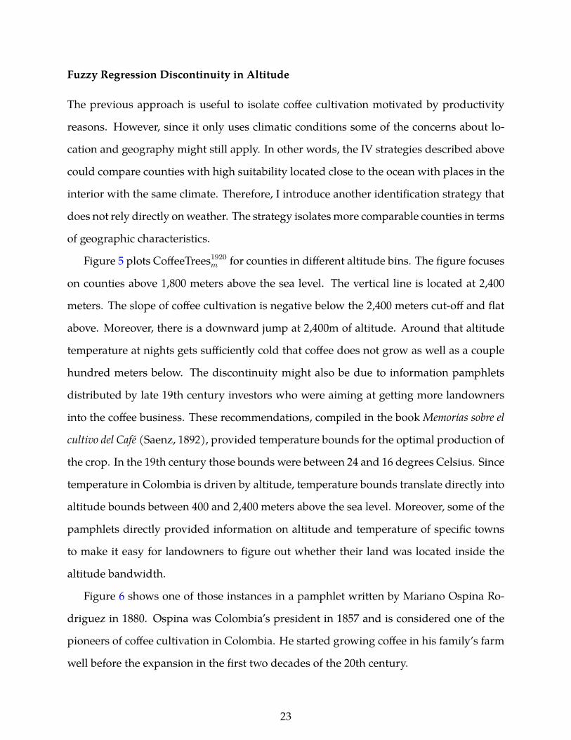
Figure 5 plots CoffeeTrees1920m for counties in different altitude bins. The figure focuses

on counties above 1,800 meters above the sea level. The vertical line is located at 2,400

meters. The slope of coffee cultivation is negative below the 2,400 meters cut-off and flat

above. Moreover, there is a downward jump at 2,400m of altitude. Around that altitude

temperature at nights gets sufficiently cold that coffee does not grow as well as a couple

hundred meters below. The discontinuity might also be due to information pamphlets

distributed by late 19th century investors who were aiming at getting more landowners

into the coffee business. These recommendations, compiled in the book Memorias sobre el

cultivo del Cafe (Saenz, 1892), provided temperature bounds for the optimal production of

the crop. In the 19th century those bounds were between 24 and 16 degrees Celsius. Since

temperature in Colombia is driven by altitude, temperature bounds translate directly into

altitude bounds between 400 and 2,400 meters above the sea level. Moreover, some of the

pamphlets directly provided information on altitude and temperature of specific towns

to make it easy for landowners to figure out whether their land was located inside the

altitude bandwidth.

Figure 6 shows one of those instances in a pamphlet written by Mariano Ospina Ro-

driguez in 1880. Ospina was Colombia’s president in 1857 and is considered one of the

pioneers of coffee cultivation in Colombia. He started growing coffee in his family’s farm

well before the expansion in the first two decades of the 20th century.

23

From Figure 5, some counties below the threshold did not grow coffee in the 1920s and

some counties above the threshold had a positive number of coffee trees. Therefore, the

setting is not one of a sharp regression discontinuity. Rather, I use the discontinuous fall in

the probability of growing coffee in 1920 as an instrument for actual coffee cultivation. In

other words, I instrument CoffeeTrees1920m with a dummy variable equal to one for counties

above the altitude threshold and a simple polynomial in altitude. This allows for coffee

cultivation to fall with altitude and even for the slope to change below and above the

threshold. Identification comes from a discontinuous jump at the threshold.

In this fuzzy regression discontinuity design (FRDD) (Angrist and Pischke, 2008), the

first stage is given by:

CoffeeTrees1920m = α1abovem + α2altitudem + α3above x altitudem + νd + ξm (4)

Where above is a dummy variable equal to one for counties above 2,400 meters of al-

titude. Altitude enters the equation centered at 2,400 meters, both linearly and interacted

with above.

The benefits of using fuzzy regression discontinuity design are evident once we com-

pare counties above and below the threshold. Figure 8 plots coefficients from OLS regres-

sions of variables on the y-axis on abovem dummy variable. Most of the coefficients are

very close to zero, with the exceptions of literacy rate in 1912 and terrain ruggedness (both

lower for counties above). Altitude is higher by construction.

Notice, however, that those means test are not necessarily all that is needed for using

the fuzzy regression discontinuity as instrument for coffee cultivation. Importantly, the

identifying assumption is that no other factor should change discontinuously at 2,400 me-

ters. Only the probability of growing coffee. To test for discontinuities in other county

characteristics, Table 3 shows the results from OLS estimation using specifications iden-

tical to equation 4, but plugging in as dependent variable all the factors represented in

24

Figure 8. There are no discontinuities for most characteristics. For manufacturing em-

ployment in 1912, the coefficient on above is marginally significant and on the opposite

direction than expected: places above, which do not grow coffee, employ a slightly lower

share of population in manufacturing in 1912.

The two different approaches (IV and FRDD) present a clear trade-off. While IV strate-

gies (FAO data and rainfall, temperature polynomial) use all the available counties, the

FRDD strategy potentially gives a more reliable estimate since it uses very comparable

“treatment” and “control” groups. Figure 7 illustrate the trade-off in terms of sample size.

Figure (a) shows the 759 counties populated in 1928 and classify them by the number of

coffee trees per square kilometer. Figure (b) highlights counties above 1,800 meters of

altitude and classifies them by their location with respect to the altitude threshold.

5 The Effect of Coffee Cultivation on Structural Transfor-

mation

This section estimates how exposure to coffee exports at the beginning of the 20th century

shaped local development and structural transformation in Colombian counties. Using

a sample of 550 IPUMS-counties, I document a sharp pattern of divergence in economic

structure between coffee producer counties and other counties. In particular, the share of

employment in manufacturing increased faster during the first part of the 20th century,

up to 1973, in counties which did not produce coffee. Meanwhile, counties which pro-

duced coffee remained mostly specialized in agriculture. I focus first on results using 1973

Census of Population. Then I show how did coffee cultivation affect economic structure at

various periods during the century. The following section expands on an important mech-

anism to explain this divergence: human capital accumulation. Finally, Section 8 estimates

the long-term impact of coffee cultivation on income and urbanization.

Coffee cultivation during the early 20th century had a negative and sizable effect on

25

structural transformation throughout the century. Results from Table 4, Panel A show an

increase of 10% in the number of coffee trees planted before 1920 led to a reduction of

around 0.05 percentage points in the share of labor force employed in manufacturing in

1973. This effect is equivalent to a reduction of 0.2% with respect to the average county. To

put it differently, going from the median level of coffee cultivation to the 75th percentile

in 1920 would decrease the 1973 share of labor force working in manufacturing by 1.6

percentage points or 8% relative to the mean. Going from the median level to the 99th

percentile would decrease manufacturing employment by 15.2% relative to the average

county.

Panel B shows the positive effect of coffee cultivation on agricultural employment. An

increase of 10% in coffee cultivation prior to 1920 would increase employment in agricul-

ture in 1973 by 0.08 percentage points, or 0.21% relative to the mean of 37% of the labor

force. The estimated magnitude of these effects is the same regardless of the method used

to instrument for coffee cultivation before 1920. Column 2 shows results using FAO cof-

fee attainable yields. Column 3 shows results using a simple polynomial in rainfall and

temperature. Results from these two methods are expected to be similar since they use

the same set of counties and exploit the same source of variation (climate). Column 4,

however, restricts the sample to counties with average altitude higher than 1,800 meters

and instruments coffee cultivation using the fuzzy regression discontinuity approach. In

other words, the set of counties “treated” by coffee availability are between 1,800 and 2,400

meters above the sea level. The fact that the results are similar between columns 2 and 3

and column 4 is evidence that the average treatment effect of coffee on structural transfor-

mation might be homogeneous, at least on dimensions related to altitude, market access,

and transportation costs.

The effect of coffee cultivation on structural transformation in terms of employment

could be driven by differences in labor force participation. I alleviate those concerns first

by measuring employment as shares of labor force. More importantly, Panel C shows

26

coffee cultivation had no significant effect on labor force participation. Even for the case

where there is a statistically significant positive effect, it is tiny. Column 2 in Panel C

implies that an increase of 10% on the number of coffee trees planted before 1920 would

increase labor force participation in 1973 by 0.07% with respect to the mean. This effect is

at least an order of magnitude smaller than the effects in Panels A and B for employment

by sector.

The estimates discussed above rely on exogenous variation provided by three differ-

ent sets of instruments. Panel D presents evidence on the relevance of the three sets of

instruments. It regresses the log of one plus the number of coffee trees in 1920 on cof-

fee attainable yield (column 2), on a polynomial on rainfall and temperature (column 3),

and on altitude, a dummy equal to one for counties above 2,400 meters of altitude, and

an interaction between the “above” dummy and altitude (column 4). All instruments are

significant and sizable. Moreover, the table also shows the F statistic for the excluded in-

struments on each one of the first stages. I do not find evidence of weak instruments.

The effect of coffee exports on employment by sector varied through the century, as Fig-

ure 9 shows. The figure complements Figure 2 by adding IV estimates from 2SLS using

attainable yields from FAO (like Column 2 in Table 1) and FRDD estimates (like Column

4). In 1912, there was no difference in sectoral employment between coffee counties and

non-coffee counties. In other words, there was no effect of potential to cultivate coffee on

the share of labor force employed in manufacturing, though there was some small posi-

tive effect on agriculture. By 1938, the effect became large and significant. It was negative

for manufacturing and positive for agriculture. This effect remained through 1973, as ex-

plained earlier. Employment in manufacturing peaked in the country in the 1970s. After

that most of the population shifted to services. Consequently, the effect of coffee cultiva-

tion in 1920 on manufacturing employment in 2005 is smaller, though significant.

In addition to using data collected from employees, coming out of Census of Popula-

tion, I use data from employers from Colombia’s first manufacturing census from 1945.

27

After the rapid growth in manufacturing in the 1930s, the country surveyed all industrial

establishments with more than five workers. It is therefore a more formal sample of man-

ufacturing establishments which might provide more information on the effect of coffee

cultivation on the process of structural transformation.

Table 5 estimates the effect of early coffee cultivation on industrial employment and

the number of industrial establishments in 1945. Column (1) reproduces results from

Table 4, Column 4, Panels B and D as reference. Columns 2 to 4 follow the same order

than results presented in Table 4. Once again, results across different instruments have

similar magnitudes and directions despite their underlying differences in sample size and

composition.

An increase of 10% on coffee trees in 1920, decreases the number of industrial establish-

ments with more than five employees in 1945 by 1.7% with respect to the mean (Panel B). It

would also decrease the share of population working in industrial establishments by 0.08

percentage points, or 16% with respect to the mean. Panel D presents the three different

first stage estimations. All specifications instrument coffee cultivation with instruments

that are not weak. Importantly, Column 4 shows evidence of the negative discontinuous

jump in the probability of growing coffee above 2,400 meters of altitude.

6 Channel: Human Capital

Colombia’s first manufacturing census provides a good setting to study whether human

capital had something to do with the effect of coffee cultivation on manufacturing. I adapt

Ciccone and Papaioannou (2009) classification for industrial sectors in the United States to

the Colombian context and divide 15 sectors compiled by 1945 Census into three groups

according to their human capital intensity. High human capital sectors include Beverages,

Instruments, Arts (Printing), and Chemicals. Medium human capital sectors include To-

bacco, Minerals, Paper, Rubber, and Metal. Finally, Low human capital sectors include

28

Leather, Textiles, Clothes, Wood, and Food. I use specification given by equation 1 for em-

ployment and number of establishments in each of the three groups. I plot the coefficients

on coffee cultivation and their standard errors. Coefficients come from a 2SLS estimation

using Coffee attainable yields from FAO as an instrument, like Table 5, Column 2.

Figure 10 shows the effect of coffee cultivation in 1920 on (a) employment in manu-

facturing and (b) number of industrial establishments in 1945 by human capital intensity.

While there is not a difference between coffee and non-coffee counties in terms of em-

ployment in more basic sectors like textiles or food, the largest difference shows up for

sectors with high intensity of human capital. In other words, the effect coffee cultivation

has on structural transformation seems to be concentrated in activities that require a more

educated labor force.

This evidence goes in line with the hypothesis described above and the models in-

troduced by Porzio and Santangelo (2019) and Caselli and Coleman II (2001). Figure 11

complements the insight from the previous evidence. It shows the difference between cof-

fee and non-coffee counties in terms of education of the labor force in 1973. Each point

represents the difference in average number of years of schooling in coffee counties minus

the average number of years of schooling in non-coffee counties for people born in each co-

hort. Though it only shows data for cohorts born from 1900 onward, there is a clear trend:

the labor force in coffee counties becomes relatively less educated in the first decades of

the 20th century. This reduction in the level of education seems to be negatively correlated

with the pattern of coffee production shown by the short-dashed line.

Using individual level data from 1973 Census of Population, I show that in fact coffee

cultivation reduced schooling and made the labor force more biased toward staying in

agriculture. Therefore, manufacturing appeared in counties which did not produce coffee.

29

Empirical Strategy

The 1973 Census of Population allows me to observe in which county and year of birth for

a 10% sample of Colombians. People born in the first half of the 20th century in counties

suitable to produce coffee were more exposed to the first large scale exporting industry

in the country. For them, the opportunity cost of attending school was higher. Moreover,

the specifics of coffee’s production function discussed on section 2 increased parent’s op-

portunity cost of sending their children to school. These incentives away from education

were potentially stronger during years when the coffee price was higher.

I test these hypotheses by estimating the effect of coffee price during school age on kids’

education and occupation as adults. I estimate the following equation:

ymcg = βCoffeeTrees1920m ∗ Price5,16c + δg + δm + δc + εmcg (5)

Where ymcg is average education or occupation outcome for gender g, cohort c, born in

county m. The coefficient of interest is β, which captures the effect of coffee price shocks

between a given cohort is 5 and 16 years old. Price5,16c is average log real coffee price in

New York between years c + 5 and c + 16. δg, δm, δc are gender, county, and cohort fixed

effects. The unit of observation is a gender by county-of-birth by cohort cell. Each cell is

weighted by the inverse of its variance.

Comparable with the empirical strategies described in section 4, I instrument Coffee

trees1920 using three different instrumental variables: coffee attainable yield, rainfall and

temperature polynomial, and a fuzzy regression discontinuity in altitude.

30

6.1 Growing Up During Coffee Price Booms Reduces Schooling and

Employment in Manufacturing for Cohorts Born in Coffee Coun-

ties

Table 6 shows the effect of coffee price shocks on educational attainment in 1973. Panel

A measures coffee shocks as the interaction between the number of coffee trees in 1920

and the log average coffee price between a cohort is 5 and 16 years old. Panel B changes

the number of coffee trees by a simple dummy equal to one for counties with some cof-

fee cultivation in 1920. Column 1 presents the OLS results. Columns 2 to 4 show results

from instrumenting coffee shocks using the variables detailed in Panel C. Interpretation

of results in Panel B is more straightforward. For simplicity, I discuss results from in-

strumenting coffee shocks with attainable yields interacted with average school age price

(Column 2): cohorts exposed to average coffee price 10% higher, born in coffee counties

accumulate 0.7% fewer years of education. Another way to put it would be to compare

1910 and 1940 cohorts. The latter cohort experienced average coffee princes during school

age 140% higher than the former due to differences on coffee prices. Therefore, the cohort

born in 1940 acquired on average 9% fewer years of education.

Panel C shows the reduced form, that is the effect of the instrument on average years

of education. Interestingly, even though the second stage is not significant and small for

column 4, the reduced form shows a coefficient with a very similar magnitude than the

2SLS results for columns 2 and 4, Panel B, but with the opposite sign, as expected. Counties

above the threshold did not produce coffee and therefore are not hit by shocks to prices.

Table 7 shows related results but looking at economic occupation and income. In gen-

eral, children born in coffee counties during periods with high coffee prices not only accu-

mulated less human capital but also were less likely to work in manufacturing as adults.

Take the result from Panel A, Column 2. Comparing again cohorts born in 1910 and 1940,

the latter cohort is almost 10% less likely to work in manufacturing due to the availability

31

of coffee cultivation that made that individual drop out of school.

Similarly, though less precisely estimated, I find a positive effect of coffee shocks during

school age on the probability of employment in agriculture as adults. Finally, in Panel C,

I show that cohorts born in coffee counties, exposed to higher coffee prices during school

age have lower household income, as measured by the first vector out of a Principal Com-

ponent Analysis on a matrix of house characteristics and durable goods.

Notice the decline in manufacturing employment is very similar than the decline in

schooling. Since schooling decisions are taken earlier (or simultaneously) than occupa-

tion decisions, I explore the effect of coffee shocks on employment in manufacturing that

is channeled through education by doing a mediation analysis proposed by Dippel et al.

(2019b). In other words, I estimate the effect of a cohort’s schooling on the share of its

members working in manufacturing in 1973 by instrumenting education using the inter-

action term between coffee attainable yields and average prices during school age, con-

ditional on coffee shocks (dummy for coffee interacted with average coffee prices during

school age). This approach provides an idea of how much of the effect of coffee prices

on occupation is acting through human capital accumulation and what fraction is going

through other channels. Specifically, I estimate the following equation:

Occup.mcg = β1Educationmcg + αCoffeeTrees1920m ∗ Price5,16c + δg + δm + δc + εmcg (6)

And instrument schooling using the following equation:

Educationmcg = γ1Attn. Yieldm ∗Price5,16c + θCoffeeTrees1920m ∗Price5,16c + δg+ δm+ δc+µmcg

(7)

This approach, however, relies on one very strong assumption: the concerns about en-

dogeneity between coffee shocks and manufacturing are the same as the concerns about

endogeneity between coffee shocks and schooling (Dippel et al., 2019a). Using this ap-

proach, the total effect is given by table 7. The share of the effect of coffee shocks on man-

32

ufacturing that goes through schooling decisions is between 80% and 96%.10 The share of

the effect depends on the measure of education used (cohort’s average years of education

or literacy rate) and on the measure of coffee cultivation (continuous or dummy). Again,

these results only hold under the assumption about the sources of endogeneity being the

same when estimating the effect of coffee shocks on education than when estimating the

effect of coffee shocks on occupation.

6.2 Supply and Demand of Schooling

So far, I have showed evidence on the negative effect of coffee cultivation on education

and manufacturing employment. My main conjecture is that coffee cultivation increases

opportunity cost of attending school. Differences in the opportunity cost of schooling gen-

erates differences in cohorts’ levels of education. As a consequence, counties producing

coffee developed lower supplies of non-agricultural workers. According to Caselli and

Coleman II (2001) and Porzio and Santangello (2019), these differences shaped the pro-

cess of structural transformation by reducing the availability of skilled workers for manu-

facturing.

In the past section I showed evidence that cohorts exposed to higher coffee prices ac-

quired lower levels of education. However, these effects of coffee cultivation and shocks

on education could come from both supply and demand. One potential explanation is

that people’s demand for schooling goes down with the possibility of producing coffee.

However, another possibility is that simply the supply of schooling in coffee counties goes

down when prices go up with respect to non-coffee counties. This might occur if, for in-

stance, landowners benefit from lower wages and a readily available labor force (Galor

et al., 2009; Galiani et al., 2008).

To explore the sources of differences in schooling between coffee and non-coffee coun-

ties, I exploit historical data on land inequality using the First Coffee Census. I observe the10Detailed results in Appendix B.4.

33

mean and median farm size in terms of coffee trees for each county with positive num-

ber of coffee trees in 1920. My conjecture is that in places with higher land inequality

within coffee landowners, the higher the market power of landowners. This would have

two consequences: first, they would have perhaps more political power to block funding

and construction of schools. Second, they could potentially behave like a monopsony and

wages would not be as responsive to changes in international price as counties with lower

inequality. In other words, if the effect of coffee shocks on education is stronger for coun-

ties with high inequality than for those with low inequality, that would be suggestive of

the effect of coffee on education being mainly driven by supply of schooling.

Table 8 shows the effect of coffee shocks on schooling, literacy, employment in manu-

facturing, employment in agriculture, and household income in 1973 for different samples.

Column 1 shows the full sample for comparison. Column 2 restricts the analysis only to

counties with at least one coffee tree in 1920. Column 3 and 4 splits the sample on Column

2 according to the median of the level of land inequality (mean/median farm).

The negative effect of coffee shocks on education and income and the positive effect on

employment in agriculture are concentrated in counties with low land inequality within

coffee landholders. This result is consistent with the hypothesis that the effect of coffee

cultivation on education is coming from changes in the demand for education. Of course,

this is only suggestive evidence given that differences in inequality might be correlated

with some of the forces behind differences in education or occupation.

I explore data on the number of schools per 10,000 inhabitants in 1951 to get at more

direct evidence on the effect of coffee cultivation on the provision of education. Unfortu-

nately, that is the only year with readily available information on provision of education at

the local level for the first half of the 20th century. Table 9 shows the effect of coffee cultiva-

tion on the number of schools, instrumenting coffee cultivation with FAO attainable yields

data. Panel A measures coffee cultivation with a dummy variable. Column 1 shows OLS

results while Column 2 shows 2SLS results from using the full sample. Coffee counties

34

have 1.05 less schools per 10,000 inhabitants than non-coffee counties in 1951. This effect

is equal to 135% of the mean of 0.64 schools per 10, 000 inhabitants on average. From Panel

B, an increase of 10% in the number of coffee trees decreases the numbers of schools per

10,000 inhabitants in 1%. Moreover, the effect has relatively the same magnitude when fo-

cusing only on counties with some coffee cultivation (Column 3). But perhaps it is more

interesting that the negative effect of coffee cultivation in 1920 on the number of schools

in 1951 is only present and stronger (thought only significant at 15%) for counties with

high levels of inequality.

In other words, these results taken together suggest that the negative effect of coffee

cultivation on human capital and structural transformation comes both from supply and

demand of education. On one hand, coffee counties have fewer schools, especially in high

inequality counties, where landowners have more power to block schooling and guarantee

a higher supply of agricultural workers. On the other hand, coffee shocks have a stronger

negative impact in counties with low inequality, where landowners have potentially less

power to fix wages they fluctuate more with international prices.

7 Channel: Linkages

I have discussed evidence of the effect of coffee cultivation on industrialization focusing

on the role of human capital accumulation, which increased the supply of non-agriculture

workers in counties not suitable to produce coffee. One concern is that the effect is coming

from counties isolated from the rest of the economy. In that scenario places with coffee

cultivation should be better off specializing on coffee in the long run even if they end up

being poorer than other counties because they would not develop manufacturing other-

wise.

Though this concern is alleviated by the comparison between coffee and non-coffee

counties in Figure 3, I explore if the effect of coffee cultivation varies with respect to how

35

connected with other sectors in the economy a county is. One way I can study the level

of linkages is by using the presence of threshing machines in some counties. Threshing

is the last process coffee cherries undergo before being exported. It is a process through

which by tumbling in a large machine, coffee cherries lose their covering husk or pergamino.

These machines were used by owners of different farms, required heavy machinery, and

expertise. Therefore, counties with this part of the coffee industry are potentially more

connected with other sectors. For example, through transportation networks, through

workers who can operate the machines, or banks who can fund their purchase, and so on.

Out of the 710 counties, 440 had some coffee cultivation in 1920. Around 120 coffee

counties also had threshing establishments. These counties had around 0.4 machines per

farm. The county with the highest number of machines had 65.

I estimate separate coefficients for the effect of producing coffee without a threshing

machine and producing coffee with threshing machines. I argue the difference between

both would give an estimate of the effect of linkages if the only difference between counties

with and without threshing is the fact that some have linkages. Table 10 shows the results.

Columns 1 and 2 replicate OLS and 2SLS estimates from section 5. Columns 3 and 4 split

the dummy for coffee cultivation in 1920 in two, according to their linkages. I find that the

effect is very close to one another. If anything, the effect of coffee on manufacturing for

counties with threshing machines is larger. The fact that threshing may not be exogenous

should give us pause to put too much weight on the coefficients.

8 Long Term Effects on Urbanization and Income

Finally, I replicate the main results using household income data for 2005 adults and coun-

ties’ poverty rate as calculated by the Social Prosperity Department. Table 11 show the

main results for all the different instruments for coffee cultivation. An increase in the

number of coffee trees in 1920 by 10% would increase poverty rate of a county in 2005 by

36

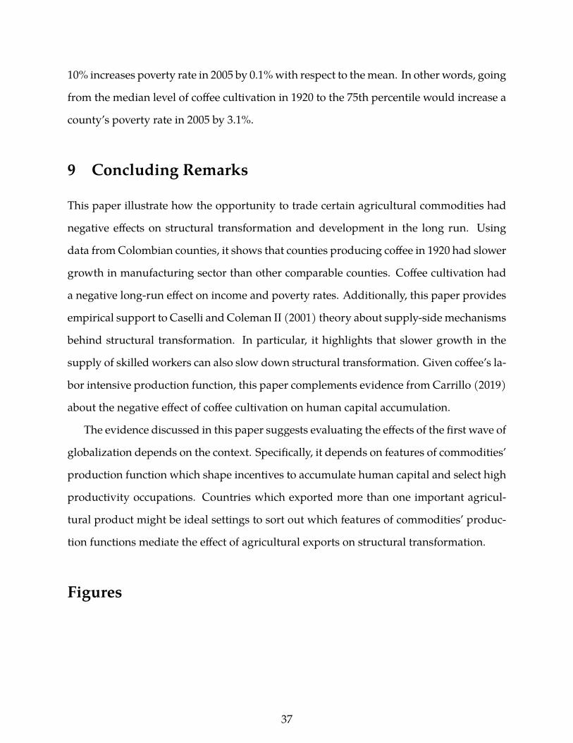
10% increases poverty rate in 2005 by 0.1% with respect to the mean. In other words, going

from the median level of coffee cultivation in 1920 to the 75th percentile would increase a

county’s poverty rate in 2005 by 3.1%.

9 Concluding Remarks

This paper illustrate how the opportunity to trade certain agricultural commodities had

negative effects on structural transformation and development in the long run. Using

data from Colombian counties, it shows that counties producing coffee in 1920 had slower

growth in manufacturing sector than other comparable counties. Coffee cultivation had

a negative long-run effect on income and poverty rates. Additionally, this paper provides

empirical support to Caselli and Coleman II (2001) theory about supply-side mechanisms

behind structural transformation. In particular, it highlights that slower growth in the

supply of skilled workers can also slow down structural transformation. Given coffee’s la-

bor intensive production function, this paper complements evidence from Carrillo (2019)

about the negative effect of coffee cultivation on human capital accumulation.

The evidence discussed in this paper suggests evaluating the effects of the first wave of

globalization depends on the context. Specifically, it depends on features of commodities’

production function which shape incentives to accumulate human capital and select high

productivity occupations. Countries which exported more than one important agricul-

tural product might be ideal settings to sort out which features of commodities’ produc-

tion functions mediate the effect of agricultural exports on structural transformation.

Figures

37

Figure 1: Patterns of Coffee Exports and Manufacturing in Colombia

(a) Value of Main Exports

0

100

200

300

400

Expo

rts in

Milli

on R

eal U

S$

1900 1910 1920 1930 1940 1950

Year

CoffeeOilBananaGold

(b) Employment in Manufacturing and Services (% of labor force)

0

.1

.2

.3

.4

Sha

re o

f Lab

or F

orce

1900 1912 1938 1973 1993 2000

Year

Manufacturing EmploymentServices Employment

Note: Figure 1a shows the real value of Colombia’s main exports in 1951 US dollars. It uses data from GRECO (2002).

Figure 1b shows shares of labor force employed in manufacturing and services. It uses data from Census of Population.

1912 and 1938 Census were digitized for this paper. 1973 and 1993 Census are available in IPUMS-international.

38

Figure 2: Correlation Coffee Cultivation and Structural Transformation

(a) Dep. Variable: Manufacturing Employment (% ofLabor Force)

-1.2

-.8

-.4

0

1912 1938 1973 2005

(b) Dep. Variable: Agricultural Employment (% ofLabor Force)

0

.2

.4

.6

.8

1912 1938 1973 2005

Note: The figures plot the coefficients of the relationship between coffee cultivation in 1920 and em-

ployment shares in manufacturing and agriculture during the 20th century. Estimates control for

gender and Department fixed effects and geographic controls. Capital cities are excluded. Lines rep-

resent 95% confidence intervals based on Conley (1999) standard errors as described in section 4.

39

Figure 3: Coffee vs. Non-Coffee Counties Comparison

Literacy, 1912

Share Manufacturing, 1912

Share Agriculture, 1912

Pop. Density, 1912

Altitude

Distance Bogota

Distance Capital

Ruggedness

Soil Quality

Native Pop., 1560

Land Disputes, 1901-31

-1 -.5 0 .5 1

Note: Figure plots standardized coefficients on an indicator variable equal to one if the county had some

coffee trees in 1920. Dependent variables are detailed on the vertical axis. For instance, the first coefficient

means coffee counties had higher literacy rate in 1912 on average than non-coffee counties. Lines represent

95% confidence intervals based on robust standard errors.

40

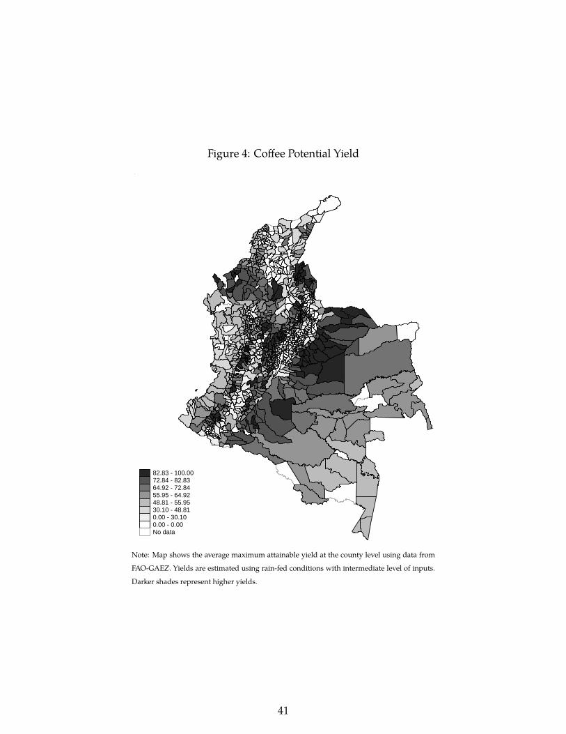
Figure 4: Coffee Potential Yield

82.83 - 100.0072.84 - 82.8364.92 - 72.8455.95 - 64.9248.81 - 55.9530.10 - 48.810.00 - 30.100.00 - 0.00No data

Note: Map shows the average maximum attainable yield at the county level using data from

FAO-GAEZ. Yields are estimated using rain-fed conditions with intermediate level of inputs.

Darker shades represent higher yields.

41

Figure 5: Discontinuity in the Probability of Coffee Cultivation at 2,400mts

0

2

4

6

8

10

log

1+ C

offe

e T

rees

(19

25)

1800 2200 2600 3000

Altitude (mts.)

Note: Figure plots average log of one plus number of coffee trees for counties grouped in equal sized bins in terms of

altitude. The figure is restricted for counties abouve 1,800 meters above sea level.

42

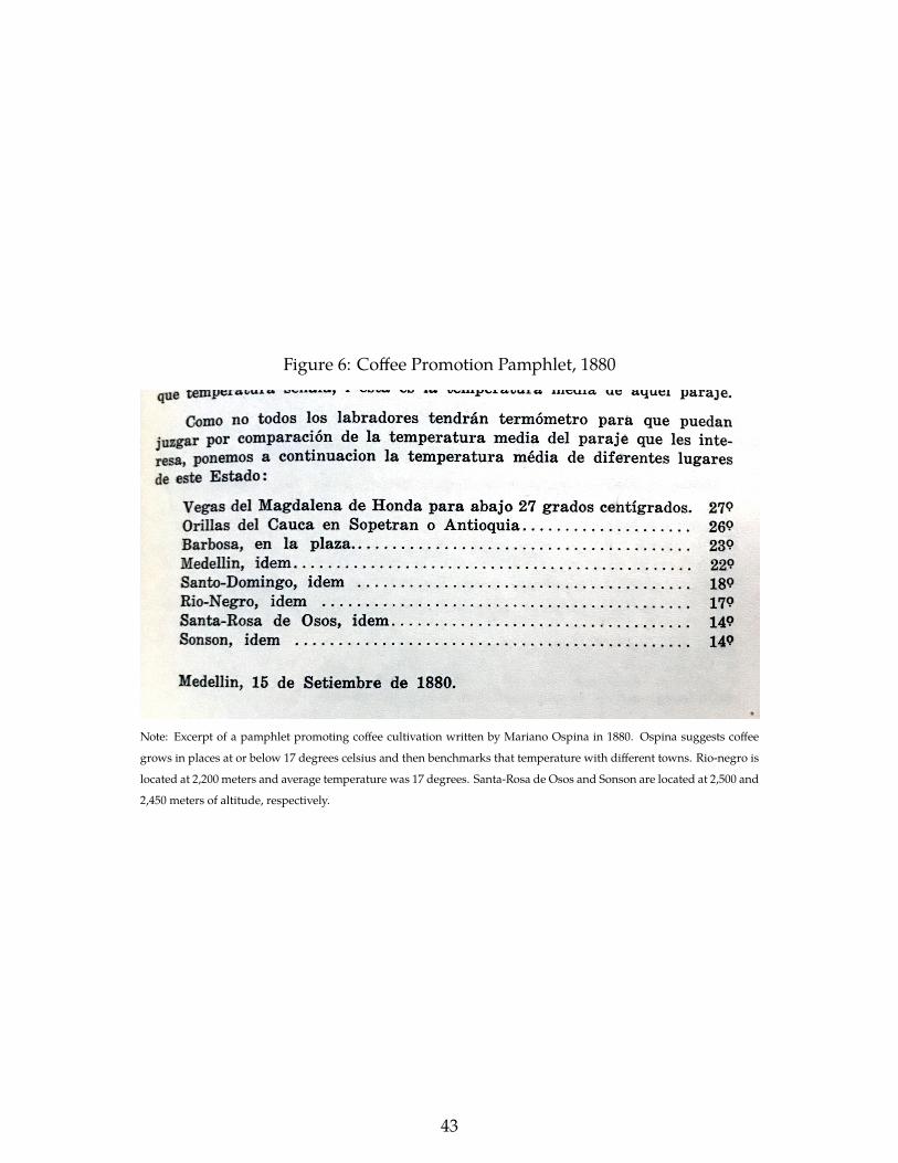
Figure 6: Coffee Promotion Pamphlet, 1880

Note: Excerpt of a pamphlet promoting coffee cultivation written by Mariano Ospina in 1880. Ospina suggests coffee

grows in places at or below 17 degrees celsius and then benchmarks that temperature with different towns. Rio-negro is

located at 2,200 meters and average temperature was 17 degrees. Santa-Rosa de Osos and Sonson are located at 2,500 and

2,450 meters of altitude, respectively.

43

Figure 7: Counties in IV and FRDD Samples

(a) IV Sample: Counties by Coffee trees per sq.km, 1920

32.4 - 437.07.3 - 32.42.1 - 7.30.2 - 2.10.0 - 0.20.0 - 0.0No data

(b) FRDD Sample: Counties above 1.8km bySide of Discontinuity

Below 2,400m

Above 2,400m

No data

Note: The maps illustrate the main samples used in each empirical strategy. Figure (a) shows the number of coffee

trees per square km in 1920 for counties with positive population in 1912. Figure (b) shows counties above 1,800 meters

classified by whether or not they are above 2,400 meters. Both maps use current county borders.

44

Figure 8: Comparison Counties Above and Below 2,400 mts. of Altitude

Literacy, 1912

Share Manufacturing, 1912

Share Agriculture, 1912

Pop. Density, 1912

Altitude

Distance Bogota

Distance Capital

Ruggedness

Soil Quality

Native Pop., 1560

Land Disputes, 1901-31

-1 -.5 0 .5 1

Note: Figure plots standardized coefficients on an indicator variable equal to one if for counties with alti-

tude higher than 2,400 meters. Dependent variables are detailed on the vertical axis. For instance, the first

coefficient means counties above 2,400 meters had lower literacy rate in 1912 on average than counties be-

tween 1,800 and 2,400 meters of altitude. Lines represent 95% confidence intervals based on robust standard

errors.

45

Figure 9: The Effect of Coffee Cultivation on Structural Transformation

(a) Dep. Variable: Manufacturing Employment (% of Labor Force)

-1.2

-.8

-.4

0

1912 1938 1973 2005

OLSIVRDD

(b) Dep. Variable: Agricultural Employment (% of Labor Force)

-.5

0

.5

1

1.5

2

1912 1938 1973 2005

OLSIVRDD

Note: The figure illustrate the effect of coffee cultivation on employment in manufacturing and agri-

culture for different years. Squares represent estimates coming from OLS regressions. Circles repre-

sent estimates from 2SLS regressions using coffee potential yields as instrument for coffee cultivation

in 1920. Diamonds display estimates using fuzzy regression discontinuity in altitude, focusing on

counties above 1.8km of altitude. All specifications control for gender and Department fixed effects

and geographic controls. Capital cities are excluded. Lines represent 95% confidence intervals based

on Conley (1999) standard errors, as described in section 4.

46

Figure 10: Effect of Coffee Cultivation on Industrialization by Human Capital Requirements in 1945

(a) Dep. Variable: Manufacturing Employment by sector (% ofpopulation)

High HK

Medium HK

Low HK

-.15 -.1 -.05 0 .05

(b) Dep. Variable: Industrial Establishments per 1,000 inhab. bysector

High HK

Medium HK

Low HK

-.15 -.1 -.05 0

Note: Each circle represents the coefficient of log coffee trees in 1920 (a) industrial employment and (b) industrial establishments in 1945. Each subfigure shows three

different models, one for each group of industrial sectors according to their human capital intensity (high, medium, low). Coefficients stem from a 2SLS regression

where log coffee trees is instrumented by coffee attainable yields. All specifications control for population in 1938 (log), distance to department’s capital, distance to

second largest market, and Department fixed effects. All specifications exclude capital cities. Lines represent 95% confidence intervals based on Conley (1999) standard

errors, as described in section 4.

47

Figure 11: Differences in Cohorts’ Schooling between Coffee and Non-Coffee Counties

10

20

30

40

50

60

Rea

l Cof

fee

Pric

e, C

ents

per

pou

nd

-.4

-.2

0

.2

.4Y

ears

of S

choo

ling

1900 1910 1920 1930 1940 1950

Cohort

Difference Schooling Coffee - Non Coffee counties

Smoothed Average

Avg. Coffee Price, 5 to 16 y.o.

Note: The circles show differences in average schooling in coffee counties and non-coffee counties for in-

dividual cohorts born in 1900 and 1950, using data from 1973 Census of Population. The long dashed line

shows the smoothed average over time of schooling differences. The short dashed line (right axis) plots the

average real coffee price between 5 and 16 years old for each cohort born between 1900 and 1950.

48

Tables

Table 1: Coffee Cultivation and Economic Structure, 1973

(1) (2) (3) (4) (5) (6)Sample restriction: Men WomenPanel A: Dep. var.: Share of Labor Force in Manufacturing, 1973log Coffee trees1920 -0.002∗∗∗ -0.002∗∗∗ -0.004∗∗∗ -0.004∗∗∗ -0.006∗∗∗ -0.003∗∗∗

(0.001) (0.001) (0.001) (0.001) (0.001) (0.001)Mean Dep. Var. 0.201 0.201 0.201 0.198 0.191 0.205r2 0.082 0.104 0.201 0.198 0.387 0.279

Panel B: Dep. var.: Share of Labor Force in Agriculture, 1973log Coffee trees1920 0.005∗∗∗ 0.005∗∗∗ 0.006∗∗∗ 0.006∗∗∗ 0.011∗∗∗ 0.002∗

(0.001) (0.001) (0.001) (0.001) (0.002) (0.001)Mean Dep. Var. 0.363 0.363 0.363 0.370 0.635 0.108r2 0.763 0.765 0.795 0.804 0.443 0.335

Panel C: Dep. var.: Share of Population in Labor Force, 1973log Coffee trees1920 -0.001∗ -0.000 -0.000 -0.000 0.002∗∗∗ -0.002∗∗∗

(0.0003) (0.0003) (0.0003) (0.0003) (0.0004) (0.0006)Mean Dep. Var. 0.531 0.531 0.531 0.530 0.891 0.169r2 0.967 0.967 0.973 0.974 0.294 0.540

Counties 563 563 563 550 548 548Geo Controls X X X X XDepartment FE X X X XCapitals X X XNote: Each Panel estimates the correlation between coffee trees in 1920 and measures of economic structurein 1973. All specifications control for population in 1973 (log). Geo controls include: distance to depart-ment’s capital, distance to second largest market, and a dummy for capital cities. Conley (1999) standarderrors as described in section 4 in parenthesis. ∗ p < 0.1, ∗∗ p < 0.05, ∗∗∗ p < 0.01

49

Table 2: Coffee Cultivation and Manufacturing in 1945

(1) (2) (3) (4)Panel A: log Industrial workers, 1945log Coffee trees1920 -0.034∗∗∗ -0.057∗∗∗ -0.065∗∗∗ -0.066∗∗∗

(0.011) (0.012) (0.015) (0.015)r2 0.343 0.395 0.443 0.360

Panel B: Industrial workers per 100 inhab., 1945log Coffee trees1920 -0.011 -0.023∗∗ -0.034∗∗∗ -0.033∗∗∗

(0.010) (0.009) (0.011) (0.011)Mean Dep. Var. 0.553 0.553 0.550 0.495r2 0.059 0.093 0.120 0.074

Panel C: log Industrial Establishments, 1945log Coffee trees1920 -0.023∗∗∗ -0.031∗∗∗ -0.033∗∗∗ -0.033∗∗∗

(0.006) (0.006) (0.008) (0.008)r2 0.378 0.443 0.489 0.359

Panel D: Industrial Establishments per 1,000 inhab., 1945log Coffee trees1920 -0.019∗∗∗ -0.023∗∗∗ -0.022∗∗∗ -0.022∗∗∗

(0.005) (0.006) (0.008) (0.008)Mean Dep. Var. 0.431 0.431 0.429 0.397r2 0.050 0.090 0.154 0.096

Counties 734 734 730 707Geo controls Y Y YDept. FE Y YDept. Capitals Y Y YNote: Each Panel presents the correlation between coffee trees in 1920 and somemeasure of industrial activity in 1945. All specifications control for populationin 1938 (log). Geo controls include: distance to department’s capital, distanceto second largest market, and a dummy for capital cities (except for column (4)where capitals are excluded). Conley (1999) standard errors as described in sec-tion 4 in parenthesis. ∗ p < 0.1, ∗∗ p < 0.05, ∗∗∗ p < 0.01

50

Table 3: Test for Other Discontinuities

(1) (2) (3) (4) (5) (6) (7) (8) (9) (10)From 1912 census: Geographic controls

Dep. Variable: Literacy Employment in Population Distance to... Terrain Soil Native Pop. LandRate Manufact. Agricult. Density Bogota Dept. Cap. Ruggedness Quality in 1560=1 Disputes

Altitude> 2, 400m -0.034 -0.016∗ -0.031 -15.047 -92.356∗ 24.137 -0.263 0.447 0.314 -0.086(0.045) (0.009) (0.025) (10.969) (51.295) (15.493) (0.385) (0.382) (0.190) (0.065)

F-stat 2.508 2.809 1.815 0.818 2.293 1.421 6.537 0.700 1.905 1.285r2 0.055 0.061 0.040 0.019 0.050 0.032 0.131 0.016 0.042 0.029Counties 134 134 134 134 134 134 134 131 134 134Note: The table tests for discontinuous jumps in counties’ characteristics at 2,400 meters. It shows results from regressing dependent variables on a dummy equal to one forcounties above 2,400 meters over the sea level, altitude, and altitude × dummy for altitude> 2, 400m. Results restrict the sample to counties above 1,800 meters. See appendix Afor variables definitions. Standard errors clustered at 60-by-60 miles grid squares in parenthesis. ∗ p < 0.1, ∗∗ p < 0.05, ∗∗∗ p < 0.01.

51

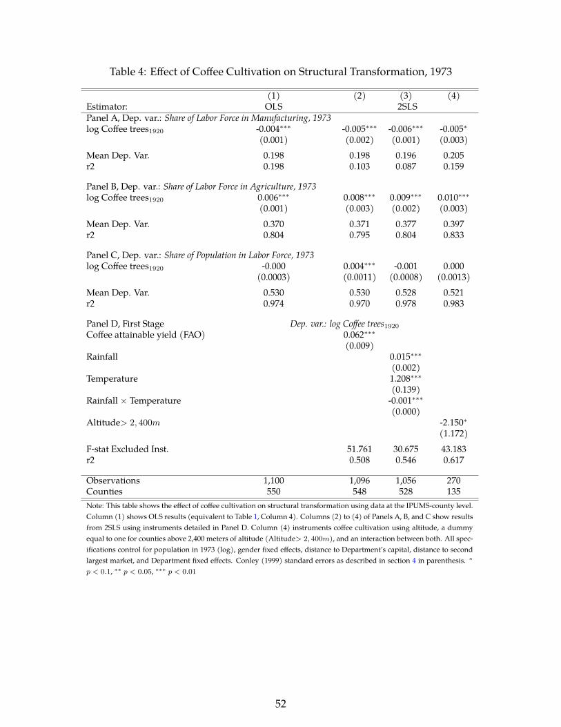
Table 4: Effect of Coffee Cultivation on Structural Transformation, 1973

(1) (2) (3) (4)Estimator: OLS 2SLSPanel A, Dep. var.: Share of Labor Force in Manufacturing, 1973log Coffee trees1920 -0.004∗∗∗ -0.005∗∗∗ -0.006∗∗∗ -0.005∗

(0.001) (0.002) (0.001) (0.003)Mean Dep. Var. 0.198 0.198 0.196 0.205r2 0.198 0.103 0.087 0.159

Panel B, Dep. var.: Share of Labor Force in Agriculture, 1973log Coffee trees1920 0.006∗∗∗ 0.008∗∗∗ 0.009∗∗∗ 0.010∗∗∗

(0.001) (0.003) (0.002) (0.003)Mean Dep. Var. 0.370 0.371 0.377 0.397r2 0.804 0.795 0.804 0.833

Panel C, Dep. var.: Share of Population in Labor Force, 1973log Coffee trees1920 -0.000 0.004∗∗∗ -0.001 0.000

(0.0003) (0.0011) (0.0008) (0.0013)Mean Dep. Var. 0.530 0.530 0.528 0.521r2 0.974 0.970 0.978 0.983

Panel D, First Stage Dep. var.: log Coffee trees1920Coffee attainable yield (FAO) 0.062∗∗∗

(0.009)Rainfall 0.015∗∗∗

(0.002)Temperature 1.208∗∗∗

(0.139)Rainfall × Temperature -0.001∗∗∗

(0.000)Altitude> 2, 400m -2.150∗

(1.172)F-stat Excluded Inst. 51.761 30.675 43.183r2 0.508 0.546 0.617

Observations 1,100 1,096 1,056 270Counties 550 548 528 135Note: This table shows the effect of coffee cultivation on structural transformation using data at the IPUMS-county level.Column (1) shows OLS results (equivalent to Table 1, Column 4). Columns (2) to (4) of Panels A, B, and C show resultsfrom 2SLS using instruments detailed in Panel D. Column (4) instruments coffee cultivation using altitude, a dummyequal to one for counties above 2,400 meters of altitude (Altitude> 2, 400m), and an interaction between both. All spec-ifications control for population in 1973 (log), gender fixed effects, distance to Department’s capital, distance to secondlargest market, and Department fixed effects. Conley (1999) standard errors as described in section 4 in parenthesis. ∗

p < 0.1, ∗∗ p < 0.05, ∗∗∗ p < 0.01

52

Table 5: 1945 IV

(1) (2) (3) (4)Estimator: OLS 2SLSPanel A: Industrial workers per 100 inhab., 1945log Coffee trees1920 -0.033∗∗∗ -0.080∗∗ -0.050∗ -0.088∗∗∗

(0.011) (0.035) (0.027) (0.029)Mean Dep. Var. 0.495 0.495 0.467 0.399r2 0.074 0.022 0.029 0.038

Panel B: Industrial Establishments per 1,000 inhab., 1945log Coffee trees1920 -0.022∗∗∗ -0.071∗∗∗ -0.061∗∗∗ -0.084∗∗∗

(0.008) (0.020) (0.020) (0.031)Mean Dep. Var. 0.397 0.397 0.400 0.505r2 0.096 -0.034 -0.006 0.003

Panel C: First Stage Dep. var.: log Coffee trees1920Coffee attainable yield (FAO) 0.065∗∗∗

(0.007)Rainfall 0.010∗∗∗

(0.001)Temperature 0.970∗∗∗

(0.101)Rainfall × Temperature -0.000∗∗∗

(0.000)Altitude> 2, 400m -2.335∗∗

(1.098)F-stat excluded inst. 97.464 35.960 31.581r2 0.570 0.585 0.426

Counties 707 706 689 250Note: This table shows the effect of coffee cultivation on on some measure of industrial activityin 1945 using data at the county level. Column (1) shows OLS results (equivalent to Table 2,Column 4). Columns (2) to (4) of Panels A and B show results from 2SLS using instrumentsdetailed in Panel C. Column (4) instruments coffee cultivation using altitude, a dummy equalto one for counties above 2,400 meters of altitude (Altitude> 2, 400m), and an interactionbetween both. All specifications control for population in 1938 (log), distance to department’scapital, distance to second largest market, and Department fixed effects. All specificationsexclude capital cities. Conley (1999) standard errors as described in section 4 in parenthesis.∗ p < 0.1, ∗∗ p < 0.05, ∗∗∗ p < 0.01

53

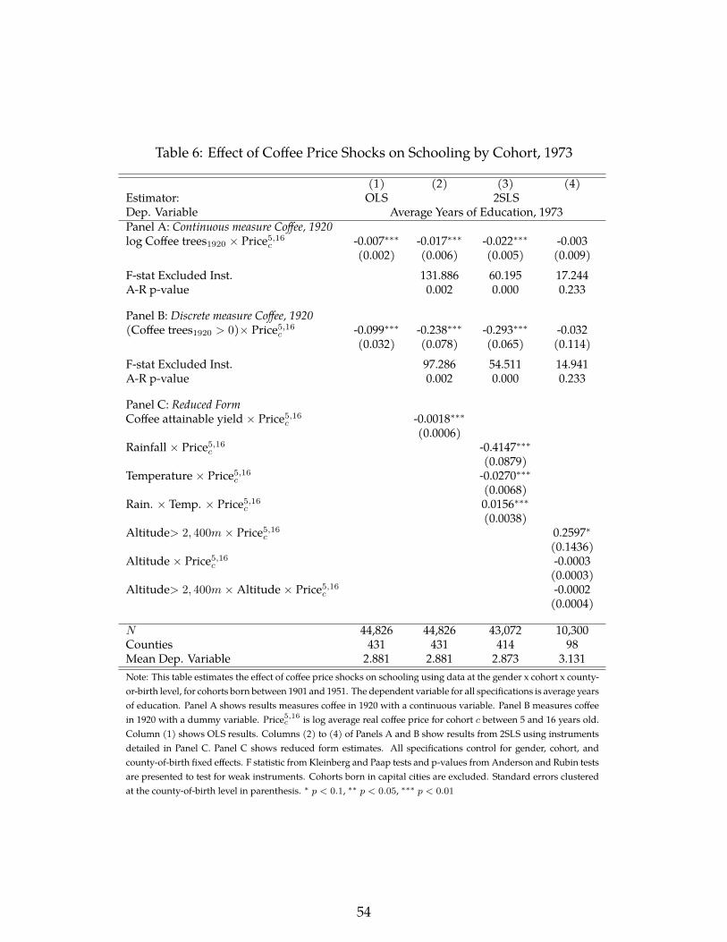
Table 6: Effect of Coffee Price Shocks on Schooling by Cohort, 1973

(1) (2) (3) (4)Estimator: OLS 2SLSDep. Variable Average Years of Education, 1973Panel A: Continuous measure Coffee, 1920log Coffee trees1920 × Price5,16c -0.007∗∗∗ -0.017∗∗∗ -0.022∗∗∗ -0.003

(0.002) (0.006) (0.005) (0.009)F-stat Excluded Inst. 131.886 60.195 17.244A-R p-value 0.002 0.000 0.233

Panel B: Discrete measure Coffee, 1920(Coffee trees1920 > 0)× Price5,16c -0.099∗∗∗ -0.238∗∗∗ -0.293∗∗∗ -0.032

(0.032) (0.078) (0.065) (0.114)F-stat Excluded Inst. 97.286 54.511 14.941A-R p-value 0.002 0.000 0.233

Panel C: Reduced FormCoffee attainable yield × Price5,16c -0.0018∗∗∗

(0.0006)Rainfall × Price5,16c -0.4147∗∗∗

(0.0879)Temperature × Price5,16c -0.0270∗∗∗

(0.0068)Rain. × Temp. × Price5,16c 0.0156∗∗∗

(0.0038)Altitude> 2, 400m × Price5,16c 0.2597∗

(0.1436)Altitude × Price5,16c -0.0003

(0.0003)Altitude> 2, 400m × Altitude × Price5,16c -0.0002

(0.0004)

N 44,826 44,826 43,072 10,300Counties 431 431 414 98Mean Dep. Variable 2.881 2.881 2.873 3.131Note: This table estimates the effect of coffee price shocks on schooling using data at the gender x cohort x county-or-birth level, for cohorts born between 1901 and 1951. The dependent variable for all specifications is average yearsof education. Panel A shows results measures coffee in 1920 with a continuous variable. Panel B measures coffeein 1920 with a dummy variable. Price5,16c is log average real coffee price for cohort c between 5 and 16 years old.Column (1) shows OLS results. Columns (2) to (4) of Panels A and B show results from 2SLS using instrumentsdetailed in Panel C. Panel C shows reduced form estimates. All specifications control for gender, cohort, andcounty-of-birth fixed effects. F statistic from Kleinberg and Paap tests and p-values from Anderson and Rubin testsare presented to test for weak instruments. Cohorts born in capital cities are excluded. Standard errors clusteredat the county-of-birth level in parenthesis. ∗ p < 0.1, ∗∗ p < 0.05, ∗∗∗ p < 0.01

54

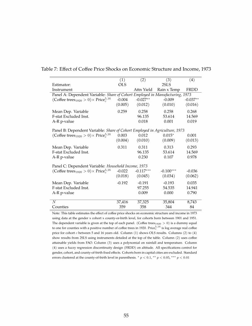
Table 7: Effect of Coffee Price Shocks on Economic Structure and Income, 1973

(1) (2) (3) (4)Estimator: OLS 2SLSInstrument Attn Yield Rain x Temp FRDDPanel A: Dependent Variable: Share of Cohort Employed in Manufacturing, 1973(Coffee trees1920 > 0)× Price5,16c -0.004 -0.027∗∗ -0.009 -0.037∗∗

(0.005) (0.012) (0.010) (0.016)Mean Dep. Variable 0.259 0.258 0.258 0.268F-stat Excluded Inst. 96.135 53.614 14.569A-R p-value 0.018 0.001 0.019

Panel B: Dependent Variable: Share of Cohort Employed in Agriculture, 1973(Coffee trees1920 > 0)× Price5,16c 0.003 0.012 0.015∗ 0.001

(0.004) (0.010) (0.009) (0.013)Mean Dep. Variable 0.311 0.311 0.313 0.293F-stat Excluded Inst. 96.135 53.614 14.569A-R p-value 0.230 0.107 0.978

Panel C: Dependent Variable: Household Income, 1973(Coffee trees1920 > 0)× Price5,16c -0.022 -0.117∗∗∗ -0.100∗∗∗ -0.036

(0.018) (0.045) (0.034) (0.062)Mean Dep. Variable -0.192 -0.191 -0.193 0.035F-stat Excluded Inst. 97.255 54.535 14.941A-R p-value 0.009 0.000 0.790

N 37,416 37,325 35,804 8,743Counties 359 358 344 84Note: This table estimates the effect of coffee price shocks on economic structure and income in 1973using data at the gender x cohort x county-or-birth level, for cohorts born between 1901 and 1951.The dependent variable is given at the top of each panel. (Coffee trees1920 > 0) is a dummy equalto one for counties with a positive number of coffee trees in 1920. Price5,16c is log average real coffeeprice for cohort c between 5 and 16 years old. Column (1) shows OLS results. Columns (2) to (4)show results from 2SLS using instruments detailed at the top of the table. Column (2) uses coffeeattainable yields from FAO. Column (3) uses a polynomial on rainfall and temperature. Column(4) uses a fuzzy regression discontinuity design (FRDD) on altitude. All specifications control forgender, cohort, and county-of-birth fixed effects. Cohorts born in capital cities are excluded. Standarderrors clustered at the county-of-birth level in parenthesis. ∗ p < 0.1, ∗∗ p < 0.05, ∗∗∗ p < 0.01

55

Table 8: Coffee Shocks and Structural Transformation by Inequality

(1) (2) (3) (4)Sample Counties: All Coffee trees> 0 Low Ineq. High Ineq.Panel A, Dep. Var.: Average Years of Schooling, 1973log Coffee trees1920 × Price5,16c -0.0073∗∗∗ -0.0005 -0.0159 0.0220

(0.0025) (0.0106) (0.0144) (0.0161)Mean Dep. Var. 2.8814 2.9576 2.9311 3.0287

Panel B, Dep. Var.: Literacy Rate, 1973log Coffee trees1920 × Price5,16c -0.2351∗∗∗ -0.6238∗∗∗ -1.0410∗∗∗ 0.1914

(0.0418) (0.1658) (0.2184) (0.2839)Mean Dep. Var. 72.7947 75.7333 75.1425 77.3802

Panel C, Dep. Var.: Share of Cohort Employed in Manufacturing, 1973log Coffee trees1920 × Price5,16c -0.0003 0.0009 0.0016 0.0010

(0.0004) (0.0013) (0.0019) (0.0024)Mean Dep. Var 0.2586 0.2600 0.2518 0.2661

Panel D, Dep. Var.: Share of Cohort Employed in Agriculture, 1973log Coffee trees1920 × Price5,16c 0.0004 0.0021∗ 0.0037∗∗ -0.0010

(0.0003) (0.0012) (0.0016) (0.0024)Mean Dep. Var 0.3106 0.3135 0.3180 0.3062

Panel E, Dep. Var.: Average Household Income, 1973log Coffee trees1920 × Price5,16c -0.0023∗ -0.0100∗ -0.0173∗∗ 0.0089

(0.0014) (0.0057) (0.0085) (0.0079)Mean Dep. Var. -0.1918 0.0334 -0.0080 0.1374

N 37,416 22,973 10,963 10,495Counties 359 220 112 108Note: This table shows correlations between coffee price shocks and outcomes in 1973 using data at the gender xcohort x county-or-birth level. It uses different county samples. Column (1) uses all counties. Column (2) restrictsto counties with some coffee trees in 1920. Columns (3) and (4) restrict the sample further to coffee counties withlower and higher (respectively) land inequality than the median coffee county. All specifications control for gender,cohort, and county-of-birth fixed effects. Cohorts born in capital cities are excluded. Standard errors clustered atthe county-of-birth level in parenthesis. ∗ p < 0.1, ∗∗ p < 0.05, ∗∗∗ p < 0.01

56

Table 9: Effect of Coffee Cultivation on Number of Schools, 1951

(1) (2) (3) (4) (5)Dep. Variable: Schools per 10,000 inhabitants, 1951Sample: All countiesEstimator: OLS 2SLS

Coffee trees1920 > 0 -0.436∗∗ -1.053∗∗(0.176) (0.415)

Counties 491 476Mean Dep. Var. 0.678 0.643F-stat Excluded Inst. 49.871r2 0.154 -0.018

Sample: All counties Coffee trees> 0 Low Ineq. High Ineq.Estimator: OLS 2SLS 2SLS 2SLS 2SLSlog Coffee trees1920 -0.036∗∗ -0.073∗∗ -0.089 0.015 -0.341

(0.014) (0.029) (0.084) (0.079) (0.214)Counties 491 476 316 147 167Mean Dep. Var. 0.678 0.643 0.627 0.530 0.715F-stat Excluded Inst. 72.457 37.934 35.803 8.747r2 0.155 0.008 0.019 0.028 -0.105Note: The tables shows the effect of coffee cultivation on the number of schools per 10,000 inhabitants in 1951using data at the IPUMS-county level. All specifications estimated using 2SLS instrument coffee cultivationwith Coffee Attainable Yields from FAO. Coffee trees1920 > 0 is a dummy equal to one for counties withpositive number of coffee trees in 1920. Column (3) restricts the sample to only counties with coffee cultiva-tion in 1920. Columns (4) and(5) further divide coffee counties by level of land inequality. All specificationscontrol for population in 1951 (log), distance to Department’s capital, distance to second largest market, andDepartment fixed effects. Conley (1999) standard errors as described in section 4 in parenthesis. ∗ p < 0.1,∗∗ p < 0.05, ∗∗∗ p < 0.01

57

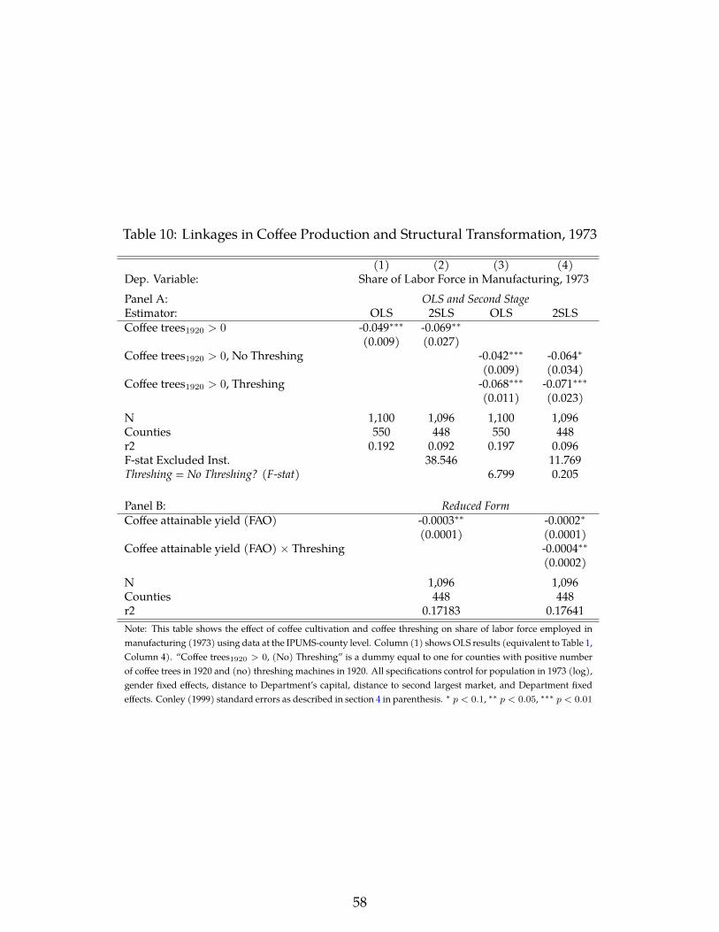
Table 10: Linkages in Coffee Production and Structural Transformation, 1973

(1) (2) (3) (4)Dep. Variable: Share of Labor Force in Manufacturing, 1973Panel A: OLS and Second StageEstimator: OLS 2SLS OLS 2SLSCoffee trees1920 > 0 -0.049∗∗∗ -0.069∗∗

(0.009) (0.027)Coffee trees1920 > 0, No Threshing -0.042∗∗∗ -0.064∗

(0.009) (0.034)Coffee trees1920 > 0, Threshing -0.068∗∗∗ -0.071∗∗∗

(0.011) (0.023)N 1,100 1,096 1,100 1,096Counties 550 448 550 448r2 0.192 0.092 0.197 0.096F-stat Excluded Inst. 38.546 11.769Threshing = No Threshing? (F-stat) 6.799 0.205

Panel B: Reduced FormCoffee attainable yield (FAO) -0.0003∗∗ -0.0002∗

(0.0001) (0.0001)Coffee attainable yield (FAO) × Threshing -0.0004∗∗

(0.0002)N 1,096 1,096Counties 448 448r2 0.17183 0.17641Note: This table shows the effect of coffee cultivation and coffee threshing on share of labor force employed inmanufacturing (1973) using data at the IPUMS-county level. Column (1) shows OLS results (equivalent to Table 1,Column 4). “Coffee trees1920 > 0, (No) Threshing” is a dummy equal to one for counties with positive numberof coffee trees in 1920 and (no) threshing machines in 1920. All specifications control for population in 1973 (log),gender fixed effects, distance to Department’s capital, distance to second largest market, and Department fixedeffects. Conley (1999) standard errors as described in section 4 in parenthesis. ∗ p < 0.1, ∗∗ p < 0.05, ∗∗∗ p < 0.01

58

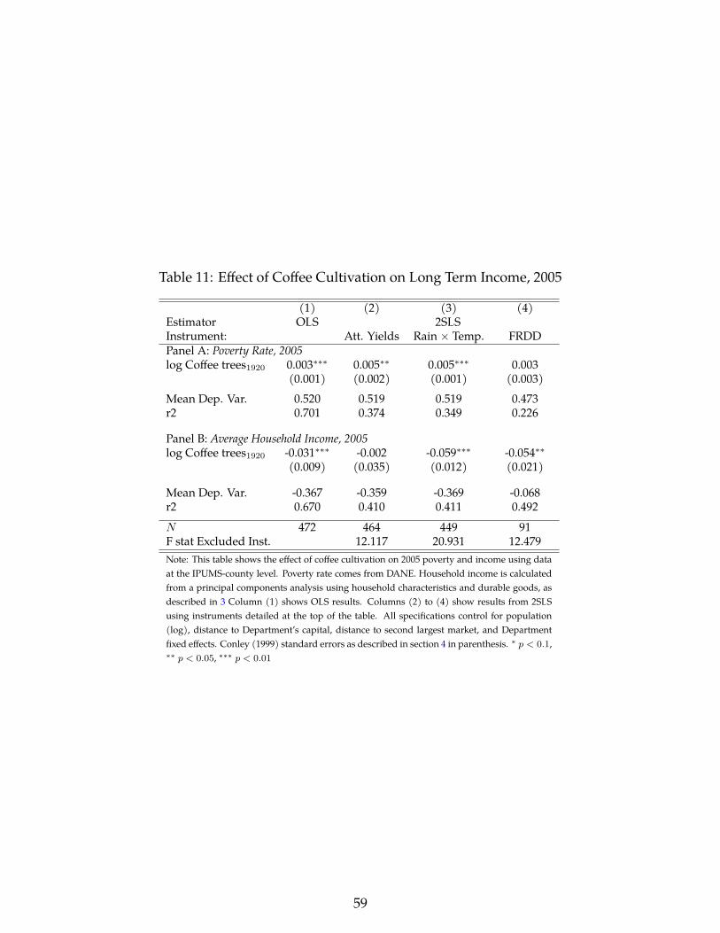
Table 11: Effect of Coffee Cultivation on Long Term Income, 2005

(1) (2) (3) (4)Estimator OLS 2SLSInstrument: Att. Yields Rain × Temp. FRDDPanel A: Poverty Rate, 2005log Coffee trees1920 0.003∗∗∗ 0.005∗∗ 0.005∗∗∗ 0.003

(0.001) (0.002) (0.001) (0.003)Mean Dep. Var. 0.520 0.519 0.519 0.473r2 0.701 0.374 0.349 0.226

Panel B: Average Household Income, 2005log Coffee trees1920 -0.031∗∗∗ -0.002 -0.059∗∗∗ -0.054∗∗

(0.009) (0.035) (0.012) (0.021)

Mean Dep. Var. -0.367 -0.359 -0.369 -0.068r2 0.670 0.410 0.411 0.492N 472 464 449 91F stat Excluded Inst. 12.117 20.931 12.479Note: This table shows the effect of coffee cultivation on 2005 poverty and income using dataat the IPUMS-county level. Poverty rate comes from DANE. Household income is calculatedfrom a principal components analysis using household characteristics and durable goods, asdescribed in 3 Column (1) shows OLS results. Columns (2) to (4) show results from 2SLSusing instruments detailed at the top of the table. All specifications control for population(log), distance to Department’s capital, distance to second largest market, and Departmentfixed effects. Conley (1999) standard errors as described in section 4 in parenthesis. ∗ p < 0.1,∗∗ p < 0.05, ∗∗∗ p < 0.01

59

References

Acemoglu, D. and Dell, M. (2010). Productivity Differences between and within Coun-tries. American Economic Journal: Macroeconomics, 2(1):169–188.

Acemoglu, D. and Guerrieri, V. (2008). Capital Deepening and Nonbalanced EconomicGrowth. Journal of Political Economy, 116(3):32.

Acevedo, K. M. and Bornacelly, I. D. (2014). Panel Municipal del CEDE. Technical Report012223, Universidad de los Andes - CEDE.

Angrist, J. D. and Pischke, J.-S. (2008). Mostly harmless econometrics: An empiricist’s com-panion. Princeton University Press.

Arango, M. (1981). Cafe e industria, 1850-1930.

Atkin, D. (2016). Endogenous Skill Acquisition and Export Manufacturing in Mexico.American Economic Review, 106(8):2046–2085.

Autor, D. H., Dorn, D., and Hanson, G. H. (2016). The China shock: Learning from labor-market adjustment to large changes in trade. Annual Review of Economics, 8:205–240.

Bazzi, S., Fiszbein, M., and Gebresilasse, M. (2017). Frontier Culture: The Roots andPersistence of ”Rugged Individualism” in the United States. Technical Report w23997,National Bureau of Economic Research, Cambridge, MA.

Bejarano, J. A. (1980). Los estudios sobre la historia del cafe en Colombia. Cuadernos deeconomıa, 1(2):115–140.

Bester, C. A., Conley, T. G., and Hansen, C. B. (2011). Inference with dependent data usingcluster covariance estimators. Journal of Econometrics, 165(2):137–151.

Bobonis, G. J. and Morrow, P. M. (2014). Labor coercion and the accumulation of humancapital. Journal of Development Economics, 108:32–53.

Brew, R. (1973). The economic development of Antioquia from 1850-1920.

Bulmer-Thomas, V. (2003). The economic history of Latin America since independence. Cam-bridge University Press.

Bustos, P., Caprettini, B., and Ponticelli, J. (2016). Agricultural Productivity and StructuralTransformation: Evidence from Brazil. American Economic Review, 106(6):1320–1365.

60

Cardoso, F. H. and Faletto, E. (1979). Dependency and development in Latin America (Depen-dencia y desarrollo en America Latina, engl.). Univ of California Press.

Carrillo, B. (2019). The Value of Time and Skill Acquisition in the Long Run: Evidencefrom Coffee Booms and Busts. Journal of Labor Economics. In Press.

Caselli, F. and Coleman II, W. J. (2001). The U.S. Structural Transformation and RegionalConvergence: A Reinterpretation. Journal of Political Economy, 109(3):584–616.

Ciccone, A. and Papaioannou, E. (2009). Human Capital, the Structure of Production, andGrowth. The Review of Economics and Statistics, 91(1):66–82.

Colella, F., Lalive, R., Sakalli, S. O., and Thoenig, M. (2019). Inference with Arbitrary Clus-tering. SSRN Scholarly Paper ID 3449578, Social Science Research Network, Rochester,NY.

Conley, T. G. (1999). GMM estimation with cross sectional dependence. Journal of Econo-metrics, 92(1):1–45.

de la Croix, D., Doepke, M., and Mokyr, J. (2018). Clans, Guilds, and Markets: Appren-ticeship Institutions and Growth in the Preindustrial Economy. The Quarterly Journal ofEconomics, 133(1):1–70.

Dippel, C., Ferrara, A., and Heblich, S. (2019a). ivmediate: Causal mediation analysis ininstrumental variables regressions.

Dippel, C., Gold, R., Heblich, S., and Pinto, R. (2019b). Mediation Analysis in IV SettingsWith a Single Instrument.

Droller, F. and Fiszbein, M. (2019). Staple Products, Linkages, and Development: Evi-dence from Argentina. Technical Report 0898-2937, National Bureau of Economic Re-search.

Dube, O. and Vargas, J. F. (2013). Commodity Price Shocks and Civil Conflict: Evidencefrom Colombia. The Review of Economic Studies, 80(4):1384–1421.

Duran, X., Musacchio, A., and Paolera, G. d. (2017). Industrial Growth in South America:Argentina, Brazil, Chile, and Colombia, 1890–2010. Oxford University Press.

Edwards, R. B. (2019). Export agriculture and rural poverty: evidence from Indonesianpalm oil.

61

Engerman, S. L. and Sokoloff, K. L. (1997). Factor endowments, institutions, and differ-ential paths of growth among new world economies. In Haber, S., editor, How LatinAmerica Fell Behind: Essays on the Economic Histories of Brazil and Mexico, 1800-1914. Stan-ford University Press.

Filmer, D. and Pritchett, L. H. (2001). Estimating Wealth Effects without ExpenditureData-or Tears: An Application to Educational Enrollments in States of India. Demogra-phy, 38(1):115–132.

Fiszbein, M. (2017). Agricultural Diversity, Structural Change and Long-run Develop-ment: Evidence from the U.S. Working Paper 23183, National Bureau of Economic Re-search.

Foster, A. and Rosenzweig, M. (2004). Agricultural Productivity Growth, Rural EconomicDiversity, and Economic Reforms: India, 1970–2000. Economic Development and CulturalChange, 52(3):509–542.

Franck, R. and Galor, O. (2017). Technology-Skill Complementarity in Early Phases ofIndustrialization. Technical Report w23197, National Bureau of Economic Research,Cambridge, MA.

Galiani, S., Heymann, D., Dabus, C., and Tohme, F. (2008). On the emergence of publiceducation in land-rich economies. Journal of Development Economics, 86(2):434–446.

Galor, O. and Moav, O. (2004). From Physical to Human Capital Accumulation: Inequalityand the Process of Development. The Review of Economic Studies, 71(4):1001–1026.

Galor, O., Moav, O., and Vollrath, D. (2009). Inequality in Landownership, the Emergenceof Human-Capital Promoting Institutions, and the Great Divergence. Review of EconomicStudies, page 37.

Gennaioli, N., La Porta, R., Lopez-de Silanes, F., and Shleifer, A. (2013). Human Capitaland Regional Development. The Quarterly Journal of Economics, 128(1):105–164.

Goldberg, P. K. and Pavcnik, N. (2007). Distributional Effects of Globalization in Devel-oping Countries. Journal of Economic Literature, 45(1):39–82.

Gollin, D., Lagakos, D., and Waugh, M. E. (2014). The Agricultural Productivity Gap. TheQuarterly Journal of Economics, 129(2):939–993.

62

GRECO (2002). El crecimiento economico colombiano en el siglo XX. Banco de la Republica.

Herrendorf, B. and Schoellman, T. (2018). Wages, Human Capital, and Barriers to Struc-tural Transformation. American Economic Journal: Macroeconomics, 10(2):1–23.

Hirschman, A. O. (1958). The strategy of economic development. Yale University Press.

Hornbeck, R. and Keskin, P. (2015). Does Agriculture Generate Local EconomicSpillovers? Short-Run and Long-Run Evidence from the Ogallala Aquifer. AmericanEconomic Journal: Economic Policy, 7(2):192–213.

Kuznets, S. (1966). Modern economic growth: findings and reflections. Nobel foundation.

LeGrand, C. (1986). Frontier expansion and peasant protest in Colombia, 1850-1936. Universityof New Mexico Press.

Lewis, A. (1955). The Theory of Economic Development. Allen and Unwin, London.

Matsuyama, K. (1992). Agricultural productivity, comparative advantage, and economicgrowth. Journal of Economic Theory, 58(2):317–334.

McGreevey, W. P. (1971). An economic history of Colombia, 1845-1930. Cambridge UniversityPress.

Mejia, J. (2018). Social networks and entrepreneurship. evidence from a historical episodeof industrialization.

Moscona, J. (2018). Agricultural development and structural change, within and acrosscountries.

Murphy, K. M., Shleifer, A., and Vishny, R. (1989). Income Distribution, Market Size, andIndustrialization. The Quarterly Journal of Economics, 104(3):537–564.

Nieto Arteta, L. E. (1971). El cafe en la sociedad colombiana.

Nunn, N. and Puga, D. (2010). Ruggedness: The Blessing of Bad Geography in Africa.The Review of Economics and Statistics, 94(1):20–36.

Ocampo, J. A. (1984). The Colombian Economy in the 1930s. In Thorp, R., editor, LatinAmerica in the 1930s: The Role of the Periphery in World Crisis, St Antony’s Series, pages117–143. Palgrave Macmillan UK, London.

63

Ocampo, J. A. (2015). Cafe, industria y macroeconomıa: ensayos de historia economica colom-biana. Fondo de Cultura Economica.

Ocampo, J. A. and Botero, M. M. (2000). Coffee and the Origins of Modern EconomicDevelopment in Colombia. In Cardenas, E., Ocampo, J. A., and Thorp, R., editors, AnEconomic History of Twentieth-Century Latin America: Volume 1 The Export Age: The LatinAmerican Economies in the Late Nineteenth and Early Twentieth Centuries, pages 55–84. Pal-grave Macmillan UK, London.

Ocampo, J. A. and Montenegro, S. (2007). Crisis mundial, proteccion e industrializacion.Editorial Norma.

O’Rourke, K. H. and Williamson, J. G. (2002). When did globalisation begin? EuropeanReview of Economic History, 6(1):23–50.

Ospina Vasquez, L. (1955). Industria y proteccion en Colombia. Medellın: ESF.

Palacios, M. (2002). Coffee in Colombia, 1850-1970. Cambridge University Press.

Parsons, J. J. (1949). Antioqueno colonization in western Colombia. University of CaliforniaPress.

Perez, S. (2017). Railroads and the rural to urban transition: Evidence from 19th-centuryArgentina. Technical report, University of California, Davis.

Porzio, T. and Santangelo, G. (2019). Does Schooling Cause Structural Transformation?In Barcelona GSE Forum Working Paper.

Prebisch, R. (1950). The economic development of Latin America. ECLAC Thinking, Se-lected Texts (1948-1998). Santiago: ECLAC, 2016. p. 45-84.

Rosenstein-Rodan, P. N. (1943). Problems of Industrialisation of Eastern and South-Eastern Europe. The Economic Journal, 53(210/211):202–211.

Ruggles, S., King, M. L., Levison, D., McCaa, R., and Sobek, M. (2003). IPUMS-international. Historical Methods: A Journal of Quantitative and Interdisciplinary History,36(2):60–65.

Saenz, N. (1892). Memoria sobre el cultivo del cafeto. Imprenta de la Luz.

64

Salvucci, R. (2006). Export-Led Industrialization. In Bulmer-Thomas, V., Coatsworth, J.,and Cortes-Conde, R., editors, The Cambridge Economic History of Latin America.

Santos Cardenas, D. (2017). From Skirts to Slacks: Female Workers and Wage Gap in theColombian Industry in 1945. SSRN Scholarly Paper ID 3040722, Social Science ResearchNetwork, Rochester, NY.

Schultz, T. W. (1964). Transforming traditional agriculture. Yale University Press.

Squicciarini, M. P. and Voigtlander, N. (2015). Human Capital and Industrialization: Ev-idence from the Age of Enlightenment. The Quarterly Journal of Economics, 130(4):1825–1883.

Sviatschi, M. M. (2018). Making a Narco: Childhood Exposure to Illegal Labor Marketsand Criminal Life Paths.

Valencia Caicedo, F. (2019). The Mission: Human Capital Transmission, Economic Persis-tence, and Culture in South America. The Quarterly Journal of Economics.

Vollrath, D. (2011). The agricultural basis of comparative development. Journal of EconomicGrowth, 16(4):343–370.

Wallerstein, I. (2011). The modern world-system I: Capitalist agriculture and the origins of theEuropean world-economy in the sixteenth century, volume 1. Univ of California Press.

Williamson, J. G. (2011). Industrial Catching Up in the Poor Periphery 1870-1975. WorkingPaper 16809, National Bureau of Economic Research.

65

Appendix A Data Appendix

Outcome Variables

Share of population in labor force: 1912 and 1938 census already included these numbersfor every county. For 1973 and 2005 census, I calculate the county-level number of adultsbetween 18 and 65 years old who answered affirmatively to the question about labor forceparticipation. I then divide by total population, taken from each census.

Share of labor force employed in manufacturing and agriculture: for 1912 and 1938census already included the number of people by occupation. For 1973 and 2005, I usethe ISCO-68 3 code classification of occupation to identify worker’s employment sector inthree broad categories: Agriculture (Occupations in the 600 ISCO-68 code), Manufactur-ing (Occupations in the 700 ISCO-68 code except for “Miners and quarrymen” (711) and“Mineral and stone treaters” (712). Occupations in the 800 code and from codes 901 to989 (inclusive)), and Services (Occupations in the 400 and 500 ISCO-68 code).

Number of manufacturing establishments per capita: Number of manufacturing es-tablishments with more than 5 employees divided by population in 1945. From 1945 In-dustrial Census (Santos Cardenas, 2017). I interpolate county level population using datafrom 1938 and 1951 census of population.

Share of population employed in industrial establishments: Number of workers inmanufacturing establishments with more than five employees divided by population in1945. From 1945 Industrial Census (Santos Cardenas, 2017). I interpolate county levelpopulation using data from 1938 and 1951 census of population.

Human capital: I measure education in 1973. I use two variables available for indi-viduals older than 5 years old. Literacy: a dummy equal to one if the individual can readand write, zero otherwise. Years of schooling: Highest year of education completed bythe individual. Ranges from 0 to 18. I then aggregate at the county-of-birth x cohort levelusing population weights.

Household income: I calculate a measure of income for households in 1973 and 2005. Iextract the first vector of a principal components analysis on a series of variables containinginformation on house quality. I use data on household characteristics to build a measureof household wealth. They are:

Electricity: a dummy equal to one if the dwelling is connected to electricity. Sewage:a dummy equal to one if the dwelling is connected to a drainage sewer system. Watersupply: a dummy equal to one if the dwelling is connected to piped water supply. Toilet:a dummy equal to one if the dwelling has either flush toilet or latrine. Floor material:a dummy equal to one if the dwelling’s floors are made of cement, tile, brick, wood, orplastic. It equals zero if the dwelling has unfinished or no floor. Roof material: a dummyequal to one if the dwelling’s roof is made of reinforced concrete or clay tile. It equals zeroif the roof is made of zinc, tin, thatch, or discarded material. Rooms per person: numberof rooms the household uses divided by the number of people in the household.

Poverty rate: share of households living below poverty line in 2005. From Acevedoand Bornacelly (2014).

66

Coffee Cultivation

The census was part of a larger project, the book “Colombia Cafetera” by Dario Monsalve,commissioned by Colombia’s Department of Commerce to promote coffee exports abroad.The book includes general information about the country, infographics, pictures, and adetailed account of coffee farms at the municipality level. I digitized information on farms’names, owners when available, and size, measured by the number of coffee trees used inproduction. For some of the smaller plantations, the census does not include the owner’sname. For some counties, there are only counts of small farms and their size. In some rarecases, the census pools together an unknown number of plantations in a single category(“Some” or “Varias’ in Spanish). The documentation on how the census was collected isnot very comprehensive and I cannot say with confidence why some counties report theirinformation pooling the smaller farms in this fashion.

Figure 12 shows the census records for the municipality of Anza in the department ofAntioquia, an instance where the three ways of reporting the information appear. Overall,the census reports information for 37,689 farms, containing 242 million coffee trees.

I use the 1928 coffee census records to build four measures at the county level. First,the total land used for coffee plantations, which is simply the sum of the individual farms’sizes. Second, the total number of farms. I measure this in two different ways to deal withthe pooled category “Some:” one, assuming “Some” is equal to one farm (lower bound),and two: assuming the farms are equal to the smallest plantation in the county for which Ihave information (upper bound). Using the example from figure 12, the number of farmsin “Some” will be, respectively, 1 and 10. Third, the number of farms allows me to measurethe average and the median farm in every county. Finally, I calculate the Gini coefficientat the county level.

Ideally, I would like to use the information on the owners’ name, because there areinstances where the same name appears as the owner of more than one plantation. Thereare, however, two obstacles for doing so. One, naming conventions in Colombia use twolast names system. The first last name is the father’s first last name, and the second lastname is the mothers’ first last name. However, the data only includes one last name. Sincelast names in Colombia are very common, I might identify two different people with thesame name as the same individual. Two, as pointed out above, there are a significantnumber of farms for which I do not know the owner’s name. For the time being, I willassume the number of plantations is equal to the number of owners in order to calculatetwo measures of Gini coefficient, one for every estimate for the number of owners.

67

Figure 12: Example from 1928 Coffee Census (Municipality of Anza, Department ofAntioquia)

Note: Columns correspond to: Plantation name, owner’s name, number of trees.

68

Appendix B Supporting Results

B.1 Main Results for 1912, 1938, and 2005

Table 12: Effect of Coffee Price Shocks on Economic Structure, 1912, 1938, and 2005

(1) (2) (3) (4) (5) (6) (7) (8) (9)Year: 1912 1938 2005Estimator: OLS 2SLS 2SLS OLS 2SLS 2SLS OLS 2SLS 2SLSInstrument Attn. Yield FRDD Attn. Yield FRDD Attn. Yield FRDD

Panel A, Dep. Var.: Share of Labor Force Employed in Manufacturinglog Coffee trees1920 -0.002∗∗∗ -0.002∗∗∗ -0.001 -0.003∗∗∗ -0.006∗∗ -0.005∗∗ -0.001∗∗∗ -0.001 -0.003∗∗

(0.001) (0.001) (0.001) (0.001) (0.003) (0.002) (0.000) (0.001) (0.002)Mean Dep. Var. 0.035 0.034 0.033 0.097 0.096 0.137 0.024 0.024 0.034r2 0.204 0.029 0.001 0.450 0.025 0.013 0.128 0.046 0.087

Panel B, Dep. Var.: Share of Labor Force Employed in Agriculturelog Coffee trees1920 0.002∗∗ 0.002 0.003∗∗ 0.006∗∗∗ 0.008∗∗∗ 0.008∗∗ 0.004∗∗∗ -0.011 0.009

(0.001) (0.002) (0.002) (0.002) (0.003) (0.003) (0.001) (0.007) (0.006)Mean Dep. Var. 0.172 0.172 0.167 0.825 0.825 0.798 0.205 0.205 0.257r2 0.218 0.033 0.071 0.267 0.073 0.039 0.476 0.315 0.408

Observations 719 698 245 713 695 250 934 898 182F stat Excluded Inst. 28.638 11.645 35.752 12.331 12.706 39.242Note: This table presents supporting results for figure 9. It shows the effect of coffee cultivation on structural transformation using dataat the IPUMS-county level. Columns (1) (4) and (7) show OLS results (equivalent to Table 1, Column 4). Columns (3) (6) and (9)instrument coffee cultivation using altitude, a dummy equal to one for counties above 2,400 meters of altitude (Altitude> 2, 400m),and an interaction between both. All specifications control for population (log), gender fixed effects, distance to Department’s capital,distance to second largest market, and Department fixed effects. Conley (1999) standard errors as described in section 4 in parenthesis.∗ p < 0.1, ∗∗ p < 0.05, ∗∗∗ p < 0.01

69

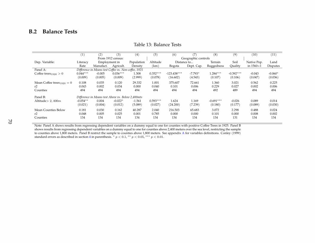
B.2 Balance Tests

Table 13: Balance Tests

(1) (2) (3) (4) (5) (6) (7) (8) (9) (10) (11)From 1912 census: Geographic controls

Dep. Variable: Literacy Employment in Population Altitude Distance to... Terrain Soil Native Pop. LandRate Manufact. Agricult. Density (km) Bogota Dept. Cap. Ruggedness Quality in 1560=1 Disputes

Panel A: Difference in Means test Coffee vs. Non-coffee, 1925Coffee trees1920 > 0 0.044∗∗∗ -0.005 0.036∗∗∗ 1.308 0.352∗∗∗ -123.438∗∗∗ -7.793∗ 1.284∗∗∗ -0.392∗∗∗ -0.043 -0.060∗

(0.009) (0.005) (0.009) (2.999) (0.078) (16.602) (4.543) (0.107) (0.106) (0.047) (0.036)Mean Coffee trees1920 = 0 0.108 0.035 0.120 29.332 1.001 375.607 72.661 1.360 3.021 0.562 0.225r2 0.043 0.002 0.034 0.000 0.040 0.101 0.006 0.229 0.027 0.002 0.006Counties 494 494 494 494 494 494 494 492 489 494 494

Panel B: Difference in Means test Above vs. Below 2,400mtsAltitude> 2, 400m -0.054∗∗ 0.004 -0.022∗ -1.561 0.593∗∗∗ 1.624 1.169 -0.691∗∗∗ -0.026 0.089 0.014

(0.021) (0.004) (0.012) (5.089) (0.027) (24.200) (7.239) (0.180) (0.177) (0.089) (0.030)Mean Counties Below 0.181 0.030 0.162 40.287 2.040 216.503 65.683 3.072 2.298 0.488 0.024r2 0.048 0.005 0.025 0.001 0.785 0.000 0.000 0.101 0.000 0.008 0.002Counties 134 134 134 134 134 134 134 134 131 134 134

Note: Panel A shows results from regressing dependent variables on a dummy equal to one for counties with positive Coffee Trees in 1925. Panel Bshows results from regressing dependent variables on a dummy equal to one for counties above 2,400 meters over the sea level, restricting the sampleto counties above 1,800 meters. Panel B restrict the sample to counties above 1,800 meters. See appendix A for variables definitions. Conley (1999)standard errors as described in section 4 in parenthesis. ∗ p < 0.1, ∗∗ p < 0.05, ∗∗∗ p < 0.01.

70

B.3 Effects by Human Capital Sector (Industrial Census, 1945)

Table 14: 1945 IV by sector

(1) (2) (3) (4) (5) (6)Dependent Variable: Industrial workers Industrial Establishments

per 100 inhab., 1945 per 1,000 inhab., 1945Instrument for Coffee Att. Yields Rain × Temp. FRDD Att. Yields Rain × Temp. FRDD

Panel A: High Human Capital Sectors

log Coffee trees1920 -0.084∗∗ -0.051∗∗∗ -0.061∗∗ -0.120∗∗∗ -0.115∗∗∗ -0.044(0.037) (0.011) (0.026) (0.024) (0.021) (0.032)

Mean Dep. Var. 0.057 0.057 0.073 0.066 0.067 0.104r2 -0.032 0.016 -0.002 -0.140 -0.119 0.067

Panel B: Medium Human Capital Sectors

log Coffee trees1920 -0.016 -0.011 -0.056 -0.023 -0.009 -0.024(0.019) (0.023) (0.036) (0.014) (0.012) (0.029)

Mean Dep. Var. 0.106 0.102 0.077 0.047 0.046 0.035r2 0.024 0.021 0.009 0.030 0.030 0.036

Panel C: Low Human Capital Sectors

log Coffee trees1920 -0.034 -0.021 -0.066∗∗ -0.070∗∗∗ -0.061∗∗ -0.083∗∗∗(0.021) (0.014) (0.028) (0.024) (0.024) (0.031)

Mean Dep. Var. 0.332 0.307 0.249 0.284 0.287 0.366r2 0.013 0.016 0.032 -0.023 -0.004 -0.000

Counties 706 689 250 706 689 250Note: Table shows effects of coffee cultivation on industrial employment and number of establishments in 1945 by sector,according to Human Capital requirement. Columns (1) and (4) use Coffee attainable yields from FAO as instrument forcoffee cultivation in 1920. Columns (2) and (5) use a polynomial on rainfall and temperature. Columns (3) and (6) use afuzzy regression discontinuity design (FRDD) on altitude. All specifications control for population in 1938 (log), distanceto department’s capital, distance to second largest market, and Department fixed effects. All specifications exclude capitalcities. Conley (1999) standard errors as described in section 4 in parenthesis. ∗ p < 0.1, ∗∗ p < 0.05, ∗∗∗ p < 0.01

71

B.4 Mediation Analysis

Table 15: Coffee Shocks and Structural Transformation by Inequality

(1) (2) (3) (4) (5)OLS 2nd. Stage OLS 2nd. Stage Red. Form

Panel A, Dep. Var: Share of Cohort Employed in Manufacturing, 1973Avg. Years of Schooling 0.0032∗∗ 0.1244∗

(0.0015) (0.0636)Literacy Rate 0.0006∗∗∗ 0.0065∗∗

(0.0001) (0.0027)Coffee attainable yield × Price5,16c -0.0002∗∗

(0.0001)Mean Dep. Var. 0.2587 0.2586 0.2585 0.2585 0.2585F-stat Excluded Inst. 8.2063 10.6217A-R test p-value 0.0179 0.0177

Panel B, Dep. Var: Share of Cohort Employed in Agriculture, 1973Avg. Years of Schooling -0.0478∗∗∗ -0.0558

(0.0013) (0.0440)Literacy Rate -0.0018∗∗∗ -0.0029

(0.0001) (0.0021)Coffee attainable yield × Price5,16c 0.0001

(0.0001)Mean Dep. Var. 0.3092 0.3105 0.3096 0.3110 0.3110F-stat Excluded Inst. 8.2063 10.6217A-R test p-value 0.2308 0.2305N 37,558 37,269 37,558 37,269 37,269Counties 361 358 361 358 358Note: This table shows the effect of education on occupation in 1973, instrumenting education using coffee pricesduring school age for cohorts born between 1901 and 1951. It uses data at the gender x cohort x county-or-birthlevel. All specifications control for gender, cohort, and county-of-birth fixed effects. Cohorts born in capital citiesare excluded. Standard errors clustered at the county-of-birth level in parenthesis. ∗ p < 0.1, ∗∗ p < 0.05, ∗∗∗

p < 0.01

72

Appendix C Robustness Checks

C.1 Extensive margin of coffee cultivation in 1920 as alternative mea-sure

Table 16: Measuring 1920 Coffee Cultivation with Extensive Margin

(1) (2) (3) (4) (5) (6) (7) (8)Year: 1912 1938 1973 2005Instrument Attn. Yield FRDD Attn. Yield FRDD Attn. Yield FRDD

Panel A, Dep. Var.: Share of Labor Force Employed in ManufacturingCoffee trees1920 > 0 -0.010 -0.018 -0.076∗∗ -0.059∗∗ -0.069∗ -0.063∗ -0.019 -0.040∗∗

(0.011) (0.012) (0.033) (0.026) (0.038) (0.036) (0.013) (0.019)Mean Dep. Var. 0.035 0.033 0.096 0.137 0.198 0.205 0.025 0.034

Panel B, Dep. Var.: Share of Labor Force Employed in AgricultureCoffee trees1920 > 0 0.050∗∗∗ 0.045∗∗ 0.108∗∗∗ 0.092∗∗ 0.111∗∗ 0.133∗∗∗ -0.157 0.151∗

(0.015) (0.018) (0.039) (0.038) (0.044) (0.032) (0.105) (0.075)Mean Dep. Var. 0.239 0.218 0.825 0.798 0.377 0.397 0.210 0.257

Panel C, Dep. Var.: Labor force participationCoffee trees1920 > 0 -0.0020 -0.0064 0.0405 0.0219 0.063∗∗∗ 0.002 -0.050 -0.041

(0.0250) (0.0178) (0.0311) (0.0236) (0.023) (0.013) (0.053) (0.035)Mean Dep. Var. 0.411 0.382 0.551 0.587 0.530 0.521 0.571 0.596

Counties 719 245 713 250 547 135 467 141F stat Excluded Inst. 26.182 11.019 31.436 11.523 14.542 12.244 11.014 9.203Note: This table presents the effect of coffee cultivation on structural transformation over the 20th century using a discretevalue equal to 1 for counties with positive coffee production in 1920, 0 otherwise. Columns (1) (3) (5) and (7) instrumentcoffee cultivation using attainable coffee yields. Columns (2) (4) (6) and (8) instrument coffee cultivation using altitude,a dummy equal to one for counties above 2,400 meters of altitude (Altitude> 2, 400m), and an interaction between both.All specifications control for population (log), gender fixed effects, distance to Department’s capital, distance to secondlargest market, and Department fixed effects. Conley (1999) standard errors as described in section 4 in parenthesis. ∗

p < 0.1, ∗∗ p < 0.05, ∗∗∗ p < 0.01

C.2 Sensitivity to Excluding Younger Cohorts

In order to test the sensibility of results to specific cohorts, I estimate results presented inSection 6.1 removing different cohorts a at a time. The following graphs show estimatesof β from equation 5 including cohorts up to years depicted in the x-axis. The preferredspecification includes cohorts between 1902 and 1052.

73

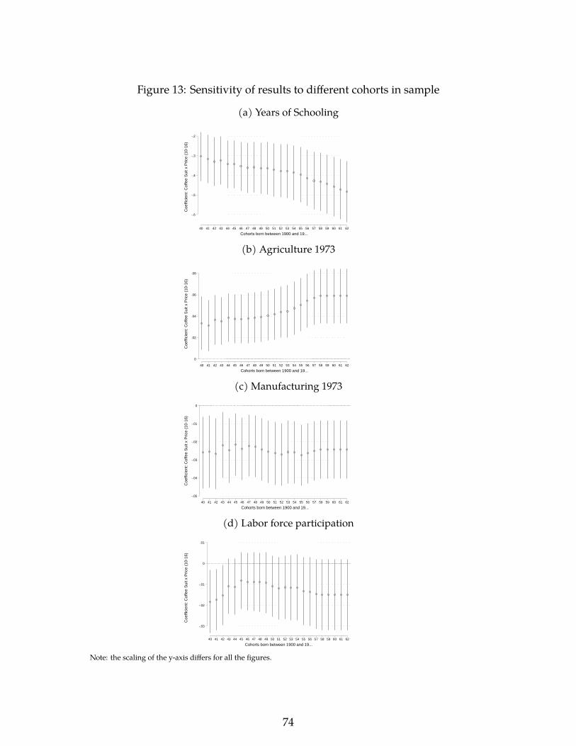
Figure 13: Sensitivity of results to different cohorts in sample

(a) Years of Schooling

-.6

-.5

-.4

-.3

-.2

Coe

ffici

ent:

Cof

fee

Sui

t x P

rice

(10-

16)

40 41 42 43 44 45 46 47 48 49 50 51 52 53 54 55 56 57 58 59 60 61 62

Cohorts born between 1900 and 19...

(b) Agriculture 1973

0

.02

.04

.06

.08

Coe

ffici

ent:

Cof

fee

Sui

t x P

rice

(10-

16)

40 41 42 43 44 45 46 47 48 49 50 51 52 53 54 55 56 57 58 59 60 61 62

Cohorts born between 1900 and 19...

(c) Manufacturing 1973

-.05

-.04

-.03

-.02

-.01

0

Coe

ffici

ent:

Cof

fee

Sui

t x P

rice

(10-

16)

40 41 42 43 44 45 46 47 48 49 50 51 52 53 54 55 56 57 58 59 60 61 62

Cohorts born between 1900 and 19...

(d) Labor force participation

-.03

-.02

-.01

0

.01

Coe

ffici

ent:

Cof

fee

Sui

t x P

rice

(10-

16)

40 41 42 43 44 45 46 47 48 49 50 51 52 53 54 55 56 57 58 59 60 61 62

Cohorts born between 1900 and 19...

Note: the scaling of the y-axis differs for all the figures.

74