Standardized Process for Filed Estimation of Unconfined Compressive Strength Using Leeb Hardness by Yassir Asiri Submitted in partial fulfilment of the requirements for the degree of Master of Applied Science at Dalhousie University Halifax, Nova Scotia February 2017 © Copyright by Yassir Asiri, 2017

Welcome message from author
This document is posted to help you gain knowledge. Please leave a comment to let me know what you think about it! Share it to your friends and learn new things together.
Transcript

Standardized Process for Filed Estimation of Unconfined
Compressive Strength Using Leeb Hardness
by
Yassir Asiri
Submitted in partial fulfilment of the requirements
for the degree of Master of Applied Science
at
Dalhousie University
Halifax, Nova Scotia
February 2017
© Copyright by Yassir Asiri, 2017
ii
TABLE OF CONTENTS
LIST OF TABLES ............................................................................................................ v
LIST OF FIGURES ........................................................................................................ vii
ABSTRACT ................................................................................................................... x
List of Abbreviations and Symbols .............................................................................. xi
ACKNOWLEDGEMENTS ............................................................................................. xiii
CHAPTER 1 INTRODUCTION ....................................................................................... 1
1.1 Overview .................................................................................................................. 1
1.2 The Aim of This Study (Objectives) ............................................................................ 2
1.3 Thesis outline ........................................................................................................... 3
CHAPTER 2 LITERATURE REVIEW ................................................................................ 5
2.1 Conventional Laboratory Methods for Rock Strength Estimation ................................ 5
2.1.1 Unconfined Compressive Strength (UCS) Test ........................................................... 5
2.1.2 Point Load Test ........................................................................................................... 6
2.2 ISRM Field Method for UCS Strength Determination .................................................. 8
2.3 Rebound Techniques for Rock Strength Determination .............................................. 9
2.3.1 Operating Principle of the Rebound Tester ................................................................ 9
2.3.1.1 Processes of Impact and Rebound ....................................................................................... 9
2.3.1.2 Residual Energy Measurement: ......................................................................................... 11
2.3.1.3 Kinetic Energy Measurement: ............................................................................................ 12
2.3.2 Schmidt Hammer Rebound Test .............................................................................. 13
2.3.3 Leeb Hardness Tester .............................................................................................. 15
2.3.3.1 Design and Operation ........................................................................................................ 16
2.3.3.2 Hardness Value ‘HLD’ Definition ........................................................................................ 17
2.4 Comparison between the Leeb Hardness Test and the Schmidt Hammer Test ........... 18
2.5 Previous Studies on Leeb Hardness Tester (LHT) ...................................................... 21
CHAPTER 3 STUDY METHODOLOGY ........................................................................... 29
iii
3.1 Lab Testing Methodology ........................................................................................ 30
3.1.1 Collection ............................................................................................................................ 30
3.1.1.1 Previously Published .......................................................................................................... 30
3.1.1.2 Quarries .............................................................................................................................. 31
3.1.2 UCS Testing ............................................................................................................... 33
3.1.2.1 Specimen Preparation (Core Sample Processes: Drilling,,) ............................................... 35
3.1.2.2 UCS Test Preparation ......................................................................................................... 42
3.1.2.4 Management ..................................................................................................................... 43
3.1.3 Rebound Test ............................................................................................................ 45
3.1.3.1 LHT and Schmidt Hammer Procedures .............................................................................. 45
3.1.3.2 Core Specimen ................................................................................................................... 46
3.1.3.3 Cubic Specimen .................................................................................................................. 47
3.2 Analysis Methods ................................................................................................... 47
3.2.1 Evaluation of Leeb Test Methodology ...................................................................... 47
3.2.1.1 Number of Impacts Comprises a Test ................................................................................ 47
3.2.1.2 Rock Specimen (Sample) Size ............................................................................................. 49
3.2.2 Leeb – UCS Correlation ............................................................................................. 50
3.2.2.1 Statistical Analysis of Data ................................................................................................. 50
3.2.2.2. Regression .......................................................................................................................... 51
3.2.2.3 Nonlinear Regression ......................................................................................................... 52
3.2.2.4 T–TEST ................................................................................................................................ 52
3.2.2.5 F–TEST ............................................................................................................................... 53
3.2.2.6 Validation of the Model .................................................................................................... 53
CHAPTER 4 LABORATORY TESTING RESULTS .............................................................. 55
4.1 Leeb Hardness Test Results ..................................................................................... 55
4.1.1 Number of Readings Averaged for a Test Result ...................................................... 55
4.1.1.1 Results of Evaluation Based on Statistical Theory .............................................................. 56
4.1.1.2 Sample Size Evaluation Based on Sampling ....................................................................... 57
4.1.2 Sample Size Effect Results ........................................................................................ 62
4.1.2.1 Results of Core and Cubic Size Effect ................................................................................. 63
4.1.2.2 Results of Scale Effect for the Mean Normalized HLD ....................................................... 65
4.2 UCS TESTING RESULTS ............................................................................................. 66
4.2.1 Schist Results ............................................................................................................ 67
4.2.2 Other Rocks............................................................................................................... 73

iv
4.3 Chapter Summary ................................................................................................... 73
CHAPTER 5 ANALYSIS ................................................................................................ 74
5.1 UCS–HLD CORRELATION .......................................................................................... 75
5.1.1 Database ................................................................................................................... 75
5.1.2 Three Rock Types ..................................................................................................... 83
5.2 Leeb Hardness Analysis ........................................................................................... 90
5.3 Comparison between HLD and Schmidt Hammer ..................................................... 92
5.4 Chapter Summary ................................................................................................... 96
CHAPTER 6 CONCLUSION and RECOMMENDATION ................................................... 97
REFERENCES ............................................................................................................ 100
Appendix 1 .............................................................................................................. 107
Appendix 2 .............................................................................................................. 126
v
LIST OF TABLES
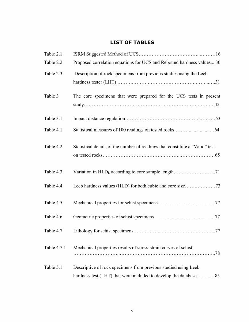
Table 2.1 ISRM Suggested Method of UCS………………………………...………16
Table 2.2 Proposed correlation equations for UCS and Rebound hardness values....30
Table 2.3 Description of rock specimens from previous studies using the Leeb
hardness tester (LHT) ……….……….………….…………….……...….31
Table 3 The core specimens that were prepared for the UCS tests in present
study…………………………………………………………….…….….42
Table 3.1 Impact distance regulation………………………………………..………53
Table 4.1 Statistical measures of 100 readings on tested rocks……….................…64
Table 4.2 Statistical details of the number of readings that constitute a “Valid” test
on tested rocks……………………….……….………..…………………65
Table 4.3 Variation in HLDL according to core sample length……………………..71
Table 4.4. Leeb hardness values (HLD) for both cubic and core size…….…………73
Table 4.5 Mechanical properties for schist specimens………………………..…….77
Table 4.6 Geometric properties of schist specimens …………………………..…..77
Table 4.7 Lithology for schist specimens……………...………………….………...77
Table 4.7.1 Mechanical properties results of stress-strain curves of schist
………………………..…………………………………………………..78
Table 5.1 Descriptive of rock specimens from previous studied using Leeb
hardness test (LHT) that were included to develop the database……..….85
vi
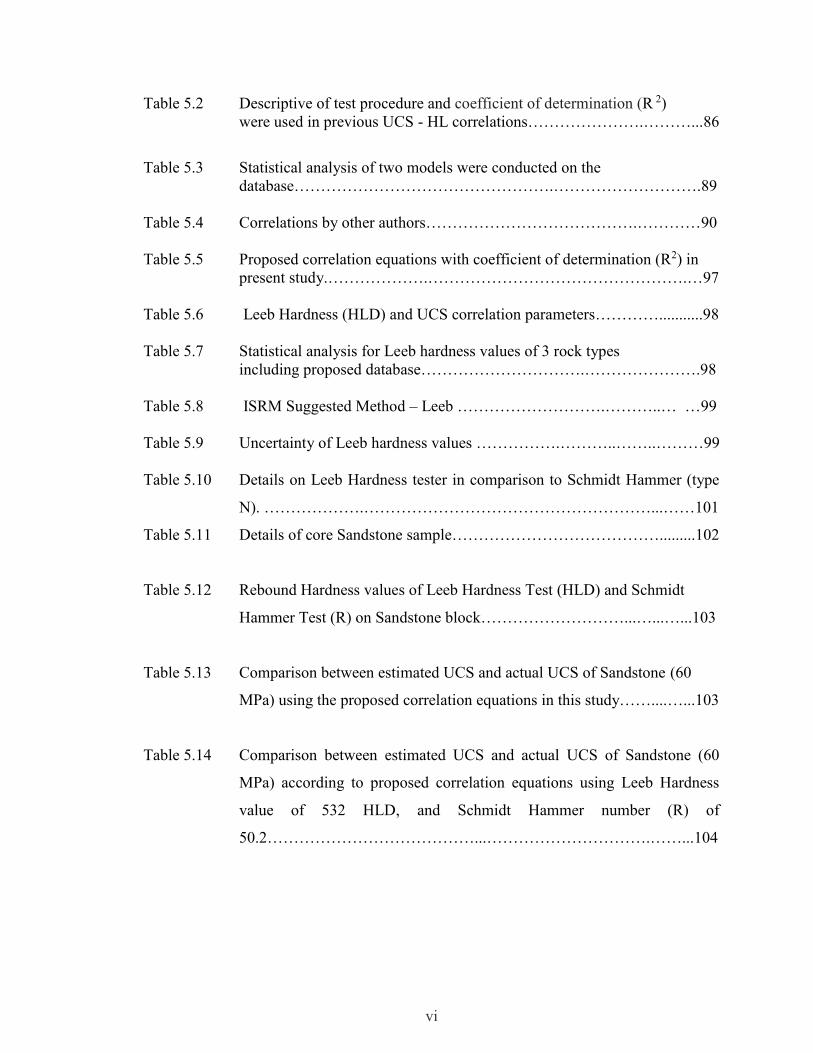
Table 5.2 Descriptive of test procedure and coefficient of determination (R 2)
were used in previous UCS - HL correlations………………….………...86
Table 5.3 Statistical analysis of two models were conducted on the
database………………………………………….……………………….89
Table 5.4 Correlations by other authors………………………………….…………90
Table 5.5 Proposed correlation equations with coefficient of determination (R2) in
present study.……………….………………………………………….…97
Table 5.6 Leeb Hardness (HLD) and UCS correlation parameters…………...........98
Table 5.7 Statistical analysis for Leeb hardness values of 3 rock types
including proposed database………………………….………………….98
Table 5.8 ISRM Suggested Method – Leeb ……………………….………..… …99
Table 5.9 Uncertainty of Leeb hardness values …………….………..……..………99
Table 5.10 Details on Leeb Hardness tester in comparison to Schmidt Hammer (type
N). ……………….………………………………………………...……101
Table 5.11 Details of core Sandstone sample………………………………….........102
Table 5.12 Rebound Hardness values of Leeb Hardness Test (HLD) and Schmidt
Hammer Test (R) on Sandstone block………………………...…...…...103
Table 5.13 Comparison between estimated UCS and actual UCS of Sandstone (60
MPa) using the proposed correlation equations in this study……....…...103
Table 5.14 Comparison between estimated UCS and actual UCS of Sandstone (60
MPa) according to proposed correlation equations using Leeb Hardness
value of 532 HLD, and Schmidt Hammer number (R) of
50.2…………………………………...………………………….……...104

vii
LIST OF FIGURES
Figure 2.1 Two specimens with the same UCS but with a different modulus of
elasticity………………………………………………….……………….19
Figure 2.2 Figure 2.2 Leeb hardness measures both the impact and rebound energy
based on the kinetic component. L and Lr are the length of a spring before
and after impact action ………………………………………….……….21
Figure 2.3 Cross - section of Leeb hardness Tester (Frank et al, 2002) …………….24
Figure 2.4 Standard voltage signals generated during the impact and rebound actions
of Leeb hardness test (Frank et al, 2002) …………………………..……25
Figure 2.5 Leeb Hardness Tester…………………………………………………….27
Figure 2.6 Leeb hardness tester vs. Schmidt hammer……………………………….29
Figure 2.7 HLD and UCS proposed correlation of previous studies………………...36
Figure 3.1 Block specimens of various rock types that were used in this study from
mining operations Eastern Canada……………………………………….41
Figure 3.2 Drilling machine……………………….…………………….…………...43
Figure 3.3 Close up of drill platform (a) and drill handles (b)………………………44
Figure 3.4 Blade saw machine……………………………….……………….……...45
Figure 3.5 Close up of vice controls into inside the wet blade saw machine….…….46
Figure 3.6 Speed settings for saw……………………………….…………………...47
Figure 3.7 Grinding machine……………………………….……………………......48
Figure 3.8 Cross feeding wheels and adjusting switches……………………………48
Figure 3.9 Adjusting switches of the grinding machine……………………….…….49
Figure 3.10 Top right panel of the grinding machine…………….…………………...49
Figure 3.11 Generic stress-strain curve……………………………….………………51

viii
Figure 3.12 UCS Machine with a sandstone sample …………………………………52
Figure 4 Core specimens of Sandstone, Granite, Dolostone, and Schist were
selected to evaluate the sample size that required to considered as a
valid test……………………………….…………………………………66
Figure 4.1 Impact Readings versus Leeb Hardness Type D (LHD) value of
Sandstone……………………………………….……….……………….67
Figure 4.2 Impact Readings versus Leeb Hardness Type D (LHD) value of
Granite……………………………………….…………………………...67
Figure 4.3 Impact Readings versus Leeb Hardness Type D (LHD) value of
Dolostone……………………………….………………………………...68
Figure 4.4 Impact Readings versus Leeb Hardness Type D (LHD) value of
Reference Hardness test block……………………………….…………..68
Figure 4.5 Impact Readings versus Leeb Hardness Type D (LHD) value of H-
Schist……………………………….…………………………………….69
Figure 4.6 Number of Readings versus Leeb Hardness Type D (LHD) value of V-
Schist……………………………….…………………………………….69
Figure 4.7 Impact Readings versus Leeb Hardness Type D (LHD) values of Granite,
Dolostone, H-Schist, V-Schist, Sandstone and Standard Hardness
Block……………………………….…………………………………….70
Figure 4.8 Non-linear increase of HLD with volume…………………………….….72
Figure 4.9 Influence of core sample size HLDL related to
HLD102mm………………………………………………….…………..…74
Figure 4.10 Schist core specimens, the strain gauge pairs were installed at the opposite
sides on them to measure the deformation, under the UCS tests…….…..76
.
Figure 4.11 Stress - Strain curves of schist specimens, using strain gauge and Linear
Variable Differential Transformer (LVDT), which are transducers to
measure the displacement for schist core specimens under UCS
tests…………………………………………………………………….....79
Figure 4.12 Schist specimens with vertical schistosity (sv1, sv2, sv3, sv4,
sv5)…………………………………………………………………..…...80
Figure 4.13 Schist specimens with horizontal schistosity (sh4, sh5, sh6, sh7, sh8, sh9,
sh10, sh11, sh12 and sh13)………... …………………………………….80
ix
Figure 4.14 Tested Schist specimens ……………….……………………..……….….8
Figure 5.1 UCS-HL correlation of the developed database……………………..…...85
Figure 5.2 HLD and UCS proposed correlation of previous studies……………..….87
Figure 5.3 Comparison between UCS-HL database correlation and the Verwaal
and Mulder (1993) results………………………………………..………89
Figure 5.4 Comparison of three rock types (Igneous, metamorphic, sedimentary)….92
Figure 5.5 Three rock types proposed correlations comparing with the proposed
database correlation…………………………………………………...….94
Figure 5.6 Metamorphic rocks proposed correlation……………………...…………95
Figure 5.7 Igneous rocks proposed correlation………………………………………96
Figure 5.8 Sedimentary proposed correlation……….…………………………..…...97
Figure 5.9 Comparison between Leeb hardness tester (LHT) and Schmidt Hammer,
type R…………………………………….…………………………..…100
Figure 5.10 Measurement range of Leeb hardness tester (LHT) and Schmidt
hammer type N…………………………………….……………………101

x
ABSTRACT
An investigation of the statistical relationship between Leeb Hardness (“D” type) values
(HLD) and unconfined compressive strength values (UCS) for different rock types was
conducted. The Leeb hardness test (LHT) procedure was evaluated by investigating the
sample size effect on HLD values and the optimum number of impacts that are required to
get a reasonable measure of the hardness of the rock specimen. For improving the UCS-
HLD correlation, the laboratory testing was carried out on rock specimens and combined
with other literature values to develop a database with a total of 311 UCS and HLD results.
Statistical analysis was carried out on the database. The predictions of the results of
correlation analysis from the tests are presented. A reasonable correlation was found to
exist between HLD and UCS. The findings from these evaluations will improve the UCS
prediction and the LHT procedure

xi
List of Abbreviations and Symbols
A0 Initial area of the specimen
D0 Initial diameter of the specimen
DF Degree of freedom
E Young’s modulus
ER Energy consumed due to frictional effects
g Gravitational constant
hi & hr Impact and rebound height
HL Leeb hardness value
HLD Hardness value of impact device D
L & Lr Length of a spring before and after impact action
L0 Initial length of the specimen
LHT Leeb hardness test
m Mass of impact body
𝑀𝐸 Margin of error
Mgs Potential gravitational energy
MSE Mean square of the error
N Total number of rebound readings
n Sample size
r Range
S Standard error of the regression
SSE Sum of squared errors of prediction
UCS Unconfined compressive strength
vr Rebound velocity
vi Impact velocity

xii
V Coefficient of variation
W Total deformation
WE1 Deformation of Elastic
Wp1 Deformation of Plastic
�̅� Sample mean
μ Population mean
λ Transformation parameter
Real standard deviation
𝜎𝑐 Ultimate compressive stress.
σpr1, σpr2, σpr3 Principal stresses
ε Strain

xiii
ACKNOWLEDGEMENTS
I would like to sincerely acknowledge Dr. Andrew Corkum and Dr. Hany El Naggar
because without them the completion of this work would not be possible. I also thank them
for all of their effort to make this thesis what it looks like now. Their guidance, support,
and advice have encouraged me to undertake the research topic “standardized process for
field estimation of Unconfined Compressive Strength (UCS) using Leeb Hardness”. I am
really grateful to them. I also would like to thank my loving family, mom, my brothers, and
especially my wife and kids for their moral support, care and patience through the duration
of my time in Canada. Also, I would like to give thanks to Jesse Keane, a technician in the
Department of Civil & Resource Engineering at Dalhousie University, who assisted me in
the laboratory during the experimental tests. Special thanks also are due for the Saudi
Arabian Cultural Bureau in Canada who supported me financially.

1
CHAPTER 1 INTRODUCTION
1.1 Overview
In rock engineering projects such as slope stability analysis, the design of underground
spaces, drilling, and rock blasting, an engineer requires knowledge of the rock strength.
Laboratory samples are idealized representations of the intact component of complex rock
masses and provide an essential starting point to determine rock mass behavior. The
Unconfined Compressive Strength (UCS) is one of the most important measures of intact
rock strength (Hoek & Martin, 2014). However, UCS tests can be time consuming to
preform. The Leeb Hardness Test (LHT) can be used to estimate the UCS quickly in the
field or laboratory environment to provide more samples and a preliminary estimation of
rock strength.
The UCS is a typical and convenient measure of rock strength, which is one of the common
parameters used in the Geotechnical Engineering field. It is a stress state where σpr1 is the
axial stress and there is zero confining stress (σpr2 = σpr3 = 0), and it is widely understood
as an index which gives a first approximation of the range of issues that are likely to be
encountered in a variety of engineering problems including roof support, pillar design, and
excavation techniques (Hoek, 1977).
The UCS of rock is a very important parameter for rock classification, rock engineering
design, and numerical modeling. In addition, for most coal mine design problems, a
reasonable approximation of the UCS is sufficient; this is due in part to the high variability
of UCS measurements in coal rock units. This property is essential for judgment about a
rock’s suitability for various construction purposes. However, determining rock UCS is
relatively time consuming and expensive for many projects. Consequently, the use of a
portable, fast and cost effective index test that can reasonably estimate UCS is desirable.
Other index field tests, such as the Schmidt Hammer (R) and the field estimation methods
outlined by the ISRM (2007) are commonly used with some acknowledged limitations.
2
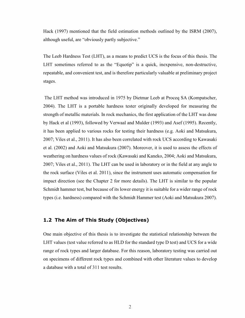
Hack (1997) mentioned that the field estimation methods outlined by the ISRM (2007),
although useful, are “obviously partly subjective.”
The Leeb Hardness Test (LHT), as a means to predict UCS is the focus of this thesis. The
LHT sometimes referred to as the “Equotip” is a quick, inexpensive, non-destructive,
repeatable, and convenient test, and is therefore particularly valuable at preliminary project
stages.
The LHT method was introduced in 1975 by Dietmar Leeb at Proceq SA (Kompatscher,
2004). The LHT is a portable hardness tester originally developed for measuring the
strength of metallic materials. In rock mechanics, the first application of the LHT was done
by Hack et al (1993), followed by Verwaal and Mulder (1993) and Asef (1995). Recently,
it has been applied to various rocks for testing their hardness (e.g. Aoki and Matsukura,
2007; Viles et al., 2011). It has also been correlated with rock UCS according to Kawasaki
et al. (2002) and Aoki and Matsukura (2007). Moreover, it is used to assess the effects of
weathering on hardness values of rock (Kawasaki and Kaneko, 2004; Aoki and Matsukura,
2007; Viles et al., 2011). The LHT can be used in laboratory or in the field at any angle to
the rock surface (Viles et al. 2011), since the instrument uses automatic compensation for
impact direction (see the Chapter 2 for more details). The LHT is similar to the popular
Schmidt hammer test, but because of its lower energy it is suitable for a wider range of rock
types (i.e. hardness) compared with the Schmidt Hammer test (Aoki and Matsukura 2007).
1.2 The Aim of This Study (Objectives)
One main objective of this thesis is to investigate the statistical relationship between the
LHT values (test value referred to as HLD for the standard type D test) and UCS for a wide
range of rock types and larger database. For this reason, laboratory testing was carried out
on specimens of different rock types and combined with other literature values to develop
a database with a total of 311 test results.
3
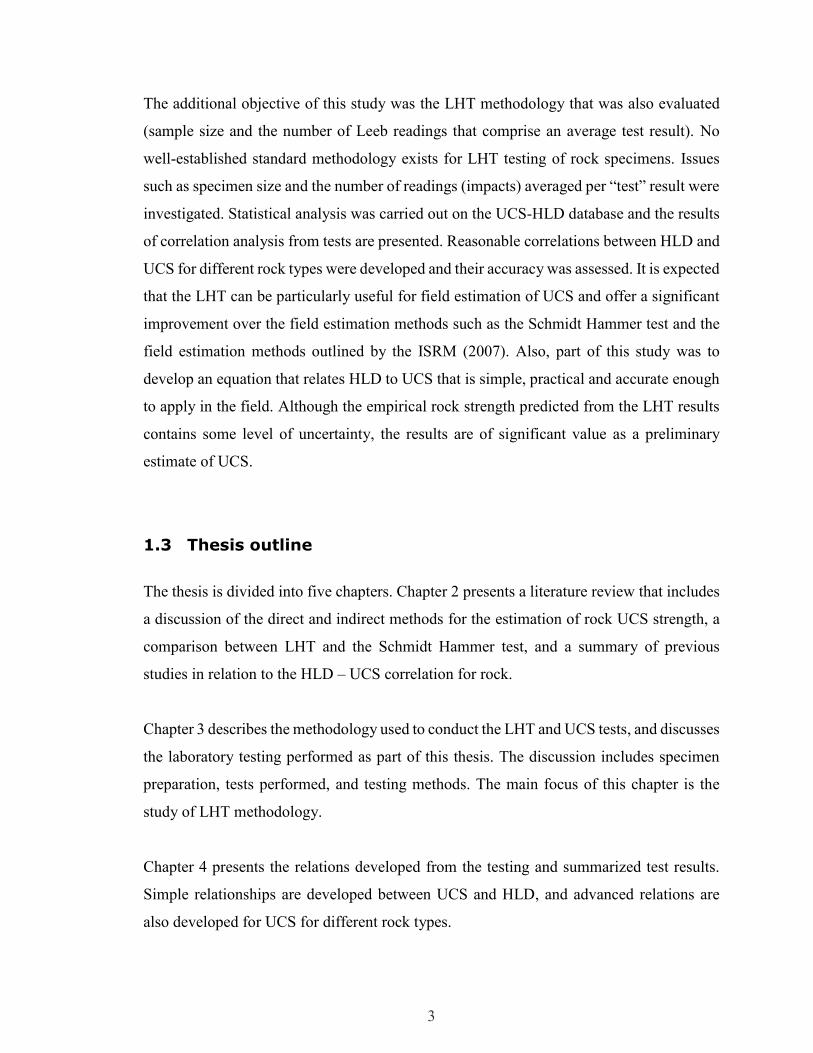
The additional objective of this study was the LHT methodology that was also evaluated
(sample size and the number of Leeb readings that comprise an average test result). No
well-established standard methodology exists for LHT testing of rock specimens. Issues
such as specimen size and the number of readings (impacts) averaged per “test” result were
investigated. Statistical analysis was carried out on the UCS-HLD database and the results
of correlation analysis from tests are presented. Reasonable correlations between HLD and
UCS for different rock types were developed and their accuracy was assessed. It is expected
that the LHT can be particularly useful for field estimation of UCS and offer a significant
improvement over the field estimation methods such as the Schmidt Hammer test and the
field estimation methods outlined by the ISRM (2007). Also, part of this study was to
develop an equation that relates HLD to UCS that is simple, practical and accurate enough
to apply in the field. Although the empirical rock strength predicted from the LHT results
contains some level of uncertainty, the results are of significant value as a preliminary
estimate of UCS.
1.3 Thesis outline
The thesis is divided into five chapters. Chapter 2 presents a literature review that includes
a discussion of the direct and indirect methods for the estimation of rock UCS strength, a
comparison between LHT and the Schmidt Hammer test, and a summary of previous
studies in relation to the HLD – UCS correlation for rock.
Chapter 3 describes the methodology used to conduct the LHT and UCS tests, and discusses
the laboratory testing performed as part of this thesis. The discussion includes specimen
preparation, tests performed, and testing methods. The main focus of this chapter is the
study of LHT methodology.
Chapter 4 presents the relations developed from the testing and summarized test results.
Simple relationships are developed between UCS and HLD, and advanced relations are
also developed for UCS for different rock types.
4
Chapter 5 contains a discussion of analysis. Included in this chapter is a discussion of the
required statistical measurements conducted on the database to determine how well the
Regression line fits the data, such as values called R-Squared (R2), and Standard Error of
the regression (S). In addition, the database is analyzed on the basis of rock types
(sedimentary, metamorphic and igneous) in subsection and the plot of UCS-HLD
correlations are presented. Classifying the HLD values based on analyzing the presented
study database was also including in this chapter before the section of the comparison
between HLD and Schmidt Hammer. The final section in this chapter presents a published
conference paper studying the LHT for sandstone specimens (see Appendix A).
Chapter 6 presents the conclusions and recommendations for future work for other
researchers who may wish to investigate the effects of sample size on HLD value.

5
CHAPTER 2 LITERATURE REVIEW
This chapter presents a review of the direct and indirect methods for the determination and
estimation of rock UCS. The first section discusses the UCS and Point Load Test (PLT).
The second section reviews the ISRM Field Methods for determination of rock strength.
The third section overviews the rebound techniques for rock strength determination, which
is included in the subsections “Operating principal of the rebound tester” and “Processes
of impact and rebound,” where the concepts are defined and related to the methods of the
hardness test. Later in the chapter, the Schmidt Hammer test and LHT are discussed
individually. The former section (LHT) is divided in two subsections, one discussing its
design and operation, and the other defining and describing the hardness value HLD. A
comparison between the LHT and the Schmidt Hammer test is discussed in the following
section. Finally, the chapter summarizes previous studies in relation to the HLD – UCS
correlation for rocks.
2.1 Conventional Laboratory Methods for Rock Strength
Estimation
2.1.1 Unconfined Compressive Strength (UCS) Test
The UCS is an important input parameter in rock engineering. It is commonly used in
engineering to determine the strength properties of a rock, soil, or other material; however,
it is not simple to perform properly and results can vary as test conditions are varied.
Specimens should be prepared and tested according to the American Society for Testing
and Materials (ASTM, 1986a) standard D4543-08 or the International Society for Rock
Mechanics (ISRM, 1981), using rock cores as cylindrical test specimens.
The test specimen should be a rock cylinder of length-to-diameter ratio in the range of 2–
2.5 with flat, smooth, and parallel ends, cut perpendicularly to the cylinder axis. Test

6
procedures are provided in ASTM D-7012 standard. Typically, a UCS test is performed on
a universal testing machine UTM. This machine designed with different capacities such as:
1000 kN or 2000 kN, and applies uniaxial load at a constant strain rate on specimens by
applying an increasing load to a cylindrical sample, until the sample fails. During the tests,
typically a load cell or a pair of strain gauges measure applied load and deformation. Both
cell and strain gauges are wired to a logging system to record. Computers are used to
continuously log the stress-strain, and the failure stress will be considered as the UCS of
specimens. Major deformation of the sample or fracture of the rock generally defines the
peak stress level achieved. Failures can range from benign compression to explosion of the
sample. UCS is often measured in MPa, which can be calculated from the following
equation in its basic definition:
σ =F
A [2 - 1]
F is the force recorded by the load frame in Newton, and A is the area of the cylindrical
surface in m2.
2.1.2 Point Load Test
The Point Load Test (PLT) is an accepted rock mechanics testing procedure and is an
attractive alternative to the UCS used for the calculation of rock strength. It is used to obtain
the strength classification (𝑰𝒔(𝟓𝟎)) of a rock material as well as the strength anisotropy
(𝑰𝒂(𝟓𝟎)) (Bell, 2013). PLT has been used in geotechnical analysis for over thirty years
(ISRM, 1985). The rock specimen can be in any form from core specimens, cut blocks, to
irregular lumps resulting in very little or no preparation at sometimes. Portable PLT
equipment provides to the UCS with a correlation factor at a lower cost, making it more
feasible to use in the field. Early studies (Bieniawski, 1975; Broch and Franklin, 1972)
were conducted on hard, strong rocks, and found that the relationship between UCS and
the point load strength could be expressed as:
7
UCS = (K) Is(50) [2 - 2]
In this equation, K is the "conversion factor." Subsequent studies found that K=24 was not
as universal as had been hoped, and that instead there appeared to be a broad range of
conversion factors. It was found that the K value varied depending on the rock type with a
range of 15 to 50 (Akram & Bakar, 2016). Consequently, it is safer to directly use 𝑰𝒔(𝟓𝟎),
as reporting the UCS without the K value when using an inappropriate K value can result
in up to 100% error (ISRM, 1985). The shape of the sample used greatly affects the
accuracy of the results. However, the relationship above is used in many of today’s projects,
replacing the standard UCS test.
Broch and Franklin (1972) reported less distribution of PLT strength test results, making it
advantageous compared to standard UCS test results. While Bieniawski (1975) reported
the opposite, Cargill and Shakoor (1990) concluded the same coefficient of variation (V)
for both tests. UCS tests showed a V of 3.1-17.1% with an average of 9.2% for different
types or rock. PLT showed a V of 4.1-24.8% with an average of 11.6%. The distribution of
points was observed to be lower at low-medium strength values and to increase as
corresponding values increase. Accordingly, they concluded that empirical equations are
better for low to medium values, as the equations become less reliable for higher strength
values.
There are many studies proposing relationships between Is(50) and UCS (Hawkins 1998;
Hawkins and Olver 1986; Romana 1999; Palchik and Hatzor 2004; Thuro and Plinninger,
2005). Tsiambaos and Sabatakakis (2004) reported that there are multiple factors, such as
composition and texture of rocks, that affect the UCS and Is(50) correlation and stated that
for soft to hard rock different conversion factors are required.

8
2.2 ISRM Field Method for UCS Strength Determination
The ISRM suggested method for field estimation of UCS has been useful in rock
engineering practice. Rock hardness can be determined by Schmidt Hammer test, UCS, the
ISRM method or LHT. Table 2.1 shows the ISRM method to estimate rock strength by
hammer blows or breaking by hand as grades ‘R’. It is used in rock mechanics to classify
rock strength in the field (Burnett, 1975).
Table 2.1 ISRM Suggested Method of UCS
Grade Term UCS
(MPa)
Field estimation method
R0 Extremely weak 0.25 – 1 Indented by thumbnail
R1 Very weak 1 – 5 Crumbles under firm blows with point of a
geological hammer, can be peeled by a pocket
knife
R2 Weak 5 – 25 Can be peeled with a pocket knife with
difficulty, shallow indentation made by firm
blow with point of a geological hammer
R3 Medium strong 25 – 50 Cannot be scraped or peeled with a pocket
knife, specimen can be fractured with a single
blow from a geological hammer
R4 Strong 50 – 100 Specimen requires more than one blow of a
geological hammer to fracture it
R5 Very strong 100 – 250 Specimen requires many blows of a geological
hammer to fracture it
R6 Extremely
strong
>250 Specimen can only be chipped with a
geological hammer
This method was based on the results of many different researchers to avoid any bias, by
taking a large number of assessments of rock strength on the same rock. Results for this
method are “obviously partly subjective” (Hack, 1996). It is standardized with a British
code (BS 5930, 1981). However, its lack of accuracy and reliability for estimating the
strength of intact rock is its limitation, and makes it highly inaccurate.

9
2.3 Rebound Techniques for Rock Strength Determination
This section overviews the rebound techniques for rock strength determination, which is
included in subsections “Operating principal of the rebound tester” and “Processes of
impact and rebound,” where the concepts are defined and related to the methods of a
hardness test. The process of measurement is divided into three main phases; the Striking
phase, the Impact phase and the Rebound phase. The residual energy has two components:
the kinetic energy component and the potential energy component, which are discussed in
individual subsections. The Schmidt Hammer test and LHT were discussed individually.
The LHT is discussed, its design and operation, and the other defining and describing the
hardness value ‘HLD’.
2.3.1 Operating Principle of the Rebound Tester
In order to understand the operating principle of the rebound tester, the processes of impact
and rebound should be defined in hardness tests.
2.3.1.1 Processes of Impact and Rebound
Typically, in performing rock hardness tests, the response of the rock material to the impact
is recorded by measuring the change in residual energy before and after rebounding. The
process is divided into three main phases (Leeb, 1986): The Striking phase, the Impact
phase and the Rebound phase.
The Striking phase is the first phase; the impact body’s potential energy is converted into
kinetic energy, either by free fall or via a spring system mechanism, and the impact tip hits
the rock sample at a specified impact velocity.
The second phase is the Impact phase; this phase is divided into two sub-phases, a
Compression phase and a Recovery phase. In the Compression phase, the impact body
depresses the test material (rock), and deforms it either plastically or elastically or both. As
10
a result, the impact body deforms plastically with some energy lost as heat. The
compression phase comes to an end once the test body reaches full stop. The moment of
maximum compression is known when velocity reaches a value of zero. In the Recovery
phase, due to elasticity forces, the two bodies move apart, as the testing body fully recovers
its elasticity. However, the test material partially recovers depending on how much energy
it has accumulated. The recovery phase is considered to be complete once the testing body
is accelerated to a rebound velocity as it leaves the test material.
The third main phase is the Rebound phase. In this phase, the present residual kinetic energy
of the testing body is converted into potential energy, which is controlled by the height of
the rebound. The impact and rebound energy equations are as follow:
Impact 𝑚𝑔ℎ𝑖 = 1
2𝑚𝑣𝑖
2 [2-3]
Rebound 𝑚𝑔ℎ𝑅 = 1
2𝑚𝑣𝑅
2 [2-4]
Where:
m = impact body mass
g = gravitational constant
ℎ𝑖, ℎ𝑅= height of impact and rebound
vi, vr = velocity of impact and rebound
mgℎ𝑅= potential energy component
1
2m𝑣𝑅
2 = kinetic energy component
In LHT, hardness is defined as the ratio between impact and rebound velocity (vi / vr)
multiplied by 1000 (Leeb, 1986). The UCS of a rock is one of the key parameters affecting
the hardness (Price, 1991). Also, the elasticity modulus (Figure 2.1) has an effect on the
harness value; by using two specimens with the same compressive strength but with a

11
different modulus of elasticity, different rebound values will be exhibited (M.
Kompatscher, 2004).
𝑊 = 𝑊𝑒1 + 𝑊𝑝1 = 𝑊𝑒2 + 𝑊𝑝2 [2-5]
In which:
𝑊 = Total deformation work
𝐸 = Young’s modulus
𝑊𝑒1&2 , 𝑊𝑝1&2
= Deformation of Elastic and Plastic
Residual energy is controlled by two effects: the yielding effect and the spring effect.
Yielding only affects the residual energy by decreasing it, unlike the spring, which can
either increase or decrease its value. As a result, it is recommended that testing specimens
are to be of a sufficient mass to eliminate both effects (Leeb, 1978).
Figure 2.1 Two specimens with the same compressive strength but with a different
modulus of elasticity (After D. Leeb, 1979).
2.3.1.2 Residual Energy Measurement:
The residual energy can be measured by either the kinetic energy component or the
potential energy component. However, there are some constraints limiting the use of one
over the other, and they are as follows:
12
The Potential energy method: The rebound height (ℎ𝑅) controls the residual energy,
limiting the measurement of some of the ranges, and thereby affecting the reliability
of the rebound values. The free fall system is only restricted to horizontally placed
materials with low impact energy, limiting it to medium-high strength material (e.g.
Schmidt Hammer). The forces of friction and gravity come into effect, especially
when a spring action instrument is being used.
The Kinetic energy method: The forces of friction and gravity do not come into
effect, making this method more accurate than the Potential energy method. The
direction in which the test is carried out is not a limiting factor. The test should be
carried out in a rapid manner to avoid interference of any of the results (Asef, 1995).
2.3.1.3 Kinetic Energy Measurement:
In this method, the LHT is the only tool known to the author that can be used. It measures
both the impact and rebound energy based on the kinetic component. This is achieved as
the device measures vi and vr, impact and rebound velocities, respectively, just before the
impact body strikes the sample material and immediately after. The ratio of the impact
velocity to the rebound velocity is then calculated and is later used to determine the
hardness value. The energy equations can be expressed as follows:
Residual energy prior to impact
½ 𝑐𝑠2 ± 𝑚𝑔𝑠 + 𝐸 = ½ 𝑚𝑣𝐴2 [2 – 6]
Residual energy after impact
½ 𝑚𝑣𝑅2 = ½ 𝑐𝑠𝑅
2 ± 𝑚𝑔𝑠𝑅 + 𝐸𝑅 [2 – 7]
Where:
m = impact body mass
13
𝑣𝑖 = impact velocity
𝑣𝑟 = rebound velocity
c = spring constant
g = gravitational constant
𝐸𝑅= energy consumed due to frictional effects along rebound track
E = energy component consumed by the frictional effects along the entire spring track
½ m𝑣𝑅2 = kinetic energy at rebound starting
½ c𝑠2 = potential residual energy of the spring system
½ m𝑣𝐴2 = impact body kinetic energy immediately before impact
mg𝑠𝑅= energy of potential residual gravitational
c𝑠𝑅2 = spring system potential energy
mgs = energy of potential gravitational
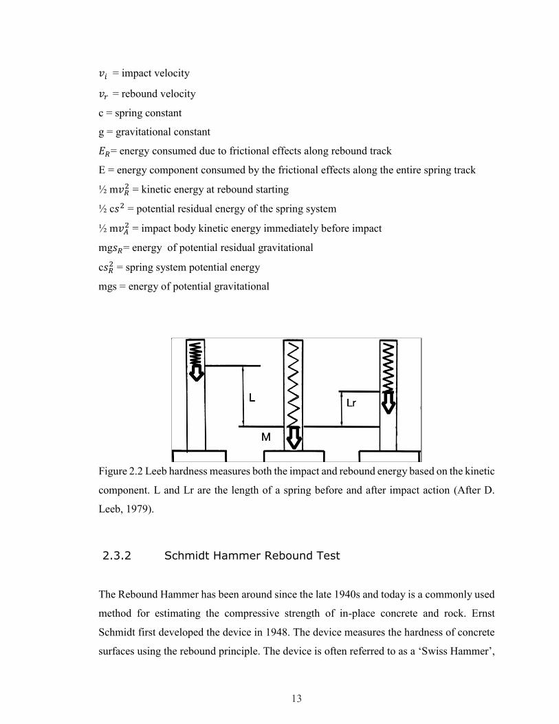
Figure 2.2 Leeb hardness measures both the impact and rebound energy based on the kinetic
component. L and Lr are the length of a spring before and after impact action (After D.
Leeb, 1979).
2.3.2 Schmidt Hammer Rebound Test
The Rebound Hammer has been around since the late 1940s and today is a commonly used
method for estimating the compressive strength of in-place concrete and rock. Ernst
Schmidt first developed the device in 1948. The device measures the hardness of concrete
surfaces using the rebound principle. The device is often referred to as a ‘Swiss Hammer’,
14
it is a standard test (ASTM D5873-05, 2005). In 1965, Miller determined that the Rebound
Hammer could correlate rock UCS using non-destructive test (NDT) methods. For its
mobility, it is used to measure specimens directly in the field, and in the lab for core
specimens starting at NX size (Edge length ≥ 60 mm). However, the rock-mass sample
must be free of any localized discontinuity, and it has to be smooth and flat for the area
below the plunger (ISRM, 1978). Since its discovery as a tool to measure rock strength,
researchers have been attempting to come up with the best recording techniques, associated
empirical formulas and the possibility of obtaining the modulus of elasticity. In 1980, Pool
and Farmer examined different techniques of hardness recording; 10 impacts are to be
performed at every point, and the peak rebound value is recorded, as well as an average of
all recorded rebound values at every point, five rebound values from single impacts of
closely spaced points are separately recorded, and then the average of the highest 3 is
calculated. Within an area with spacing of at least 25mm, 15 rebound values are recorded;
the highest 10 values are averaged within an area of 100 mm2, where 10 rebound values
are recorded. All values are averaged after the elimination of ±5 cut-off values (Proceq,
1977). An average of 9-25 single impact rebound values are used to calculate the average,
standard deviation, range, and the variation. Using a plunger diameter as a spacer, 20
rebound values are recorded from single impacts, and the highest 10 values are averaged
after eliminating any values taken from cracked rock-specimens.
Hucka’s methods (Hucka, 1965) were the accepted technique for recording, unlike all
others that were based on the single impact method on different areas. Pool and Farmer
carried out further field experiments by conducting an intensive testing program in a
shallow coal mine in order to conclude the best recording technique. The team was split
into two groups; the first group carried out tests on three series of rocks. In the first 2 series,
testing was carried out 10 times at the same point; however, it was done 15 times in the
third series. Tests were carried out on a closely packed grid (200 𝑚𝑚2, 4×4 grid). The
second group performed tests by carrying out 16 impacts, each at a one-meter interval.
Statistical analysis showed a normal distribution of: rebound values were consistent, with
slight variations in the first 3-4 impacts. Hence, they concluded that 5 successive impacts
are to be carried out before they obtain the peak value.
15
Sachpazis (1990) used the Schmidt Hammer test to determine the UCS and Young’s
modulus of carbonate rocks in Greece. He reported linear correlations as the best choices
for rebound values, and putting UCS against Young’s modulus, he obtained the following
coefficient of determinations (𝑅2) of 0.7764 and 0.8151; r = 0.881 and 0.903 respectively.
For application to assess the degree of rock weathering. Sjoberg and Broadbent (1991) used
the Schmidt Hammer test to estimate the alteration and degree of rock weathering.
McCarrol (1991) has reported a strong negative correlation between rebound values and
the degree of weathering.
From the previous experiments, it is confirmed that the Schmidt hammer is an applicable
tool to be used to predict rock-mass properties. However, it cannot provide one empirical
equation with the desired accuracy for all different rock-types. Kolaiti and Papadopoulus
(1993) noticed that the correction of the hammer direction is unnecessary for all cases.
Inaccuracies during measurement of material response and intrinsic inaccuracy of rebound
methods occur due to the interference of effected factors.
2.3.3 Leeb Hardness Tester
The Leeb hardness tester is a fairly new measuring hardness device. Recently, it has been
applied to various rocks for testing their hardness (Aoki and Matsukura, 2007; Viles et al.,
2011), and it can also be correlated with rock UCS according to Kawasaki et al. (2002) and
Aoki and Matsukura (2007). Moreover, it is used to assess the weathering effects on
hardness values (Kawasaki and Kaneko, 2004; Aoki and Matsukura, 2007; Viles et al.,
2011). The LHT can be used in laboratory or the field at any angle (Viles et al. 2011), since
the instrument uses automatic compensation for direction of impact (Yilmaz, 2012). It is
suitable for applications to cover a wider range of rock hardness compared with the Schmidt
hammer (Aoki and Matsukura 2007).
16
2.3.3.1 Design and Operation
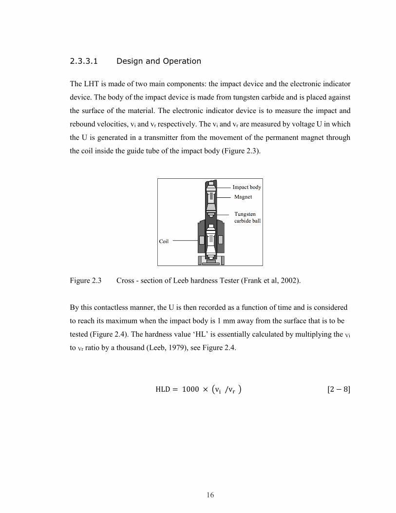
The LHT is made of two main components: the impact device and the electronic indicator
device. The body of the impact device is made from tungsten carbide and is placed against
the surface of the material. The electronic indicator device is to measure the impact and
rebound velocities, vi and vr respectively. The vi and vr are measured by voltage U in which
the U is generated in a transmitter from the movement of the permanent magnet through
the coil inside the guide tube of the impact body (Figure 2.3).
Figure 2.3 Cross - section of Leeb hardness Tester (Frank et al, 2002).
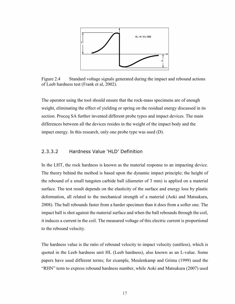
By this contactless manner, the U is then recorded as a function of time and is considered
to reach its maximum when the impact body is 1 mm away from the surface that is to be
tested (Figure 2.4). The hardness value ‘HL’ is essentially calculated by multiplying the Vi
to Vr ratio by a thousand (Leeb, 1979), see Figure 2.4.
HLD = 1000 × (vi /vr ) [2 − 8]
17
Figure 2.4 Standard voltage signals generated during the impact and rebound actions
of Leeb hardness test (Frank et al, 2002).
The operator using the tool should ensure that the rock-mass specimens are of enough
weight, eliminating the effect of yielding or spring on the residual energy discussed in its
section. Proceq SA further invented different probe types and impact devices. The main
differences between all the devices resides in the weight of the impact body and the
impact energy. In this research, only one probe type was used (D).
2.3.3.2 Hardness Value ‘HLD’ Definition
In the LHT, the rock hardness is known as the material response to an impacting device.
The theory behind the method is based upon the dynamic impact principle; the height of
the rebound of a small tungsten carbide ball (diameter of 3 mm) is applied on a material
surface. The test result depends on the elasticity of the surface and energy loss by plastic
deformation, all related to the mechanical strength of a material (Aoki and Matsukura,
2008). The ball rebounds faster from a harder specimen than it does from a softer one. The
impact ball is shot against the material surface and when the ball rebounds through the coil,
it induces a current in the coil. The measured voltage of this electric current is proportional
to the rebound velocity.
The hardness value is the ratio of rebound velocity to impact velocity (unitless), which is
quoted in the Leeb hardness unit HL (Leeb hardness), also known as an L-value. Some
papers have used different terms; for example, Meulenkamp and Grima (1999) used the
“RHN” term to express rebound hardness number, while Aoki and Matsukura (2007) used

18
the L-value term for a single impact “Ls”. The HLD denotes testing with the D device,
which can be described as:
HLD =V rebound
V impactX1000 [2 − 9]
In this study, the LHT (“D” type) was used to predict the UCS for core specimens. There
is still no established testing procedure for using the LHT to predict UCS on rocks.
Therefore, the single impact method (12 impacts) on the core specimens (Daniels et al.,
2012) is used on core specimens. The maximum and minimum reading is excluded, and the
average of the 10 remaining readings are used. The averaged Leeb hardness readings are
correlated with the UCS-test. The results show that the LHT can be particularly useful for
estimating the UCS with some level of uncertainty. Moreover, to get a reasonable measure
of the “Statistically representative” hardness of a sample rock, the LHT methodology was
examined by quantifying sample size and the number of Leeb readings (CHAPTER 4).
2.4 Comparison between the Leeb Hardness Test and the
Schmidt Hammer Test
Both the LHT and Schmidt hammer are rebound-measuring devices. The Schmidt hammer
follows traditional static tests where the test is uniformly loaded, while the LHT follows
dynamic testing methods that apply an impulsive load. The Schmidt hammer is the
traditional method that is based on clear physical indentation; it measures the distance of
rebound after a plunger hits the material surface. In contrast, the LHT (Figure 5) is a lighter,
smaller and non-destructive device that leaves a little damage with an indentation of just
~0.5 mm, which allows for an advantageous measurement for a thin layer. LHT is also
faster: the duration of the test is only seconds.
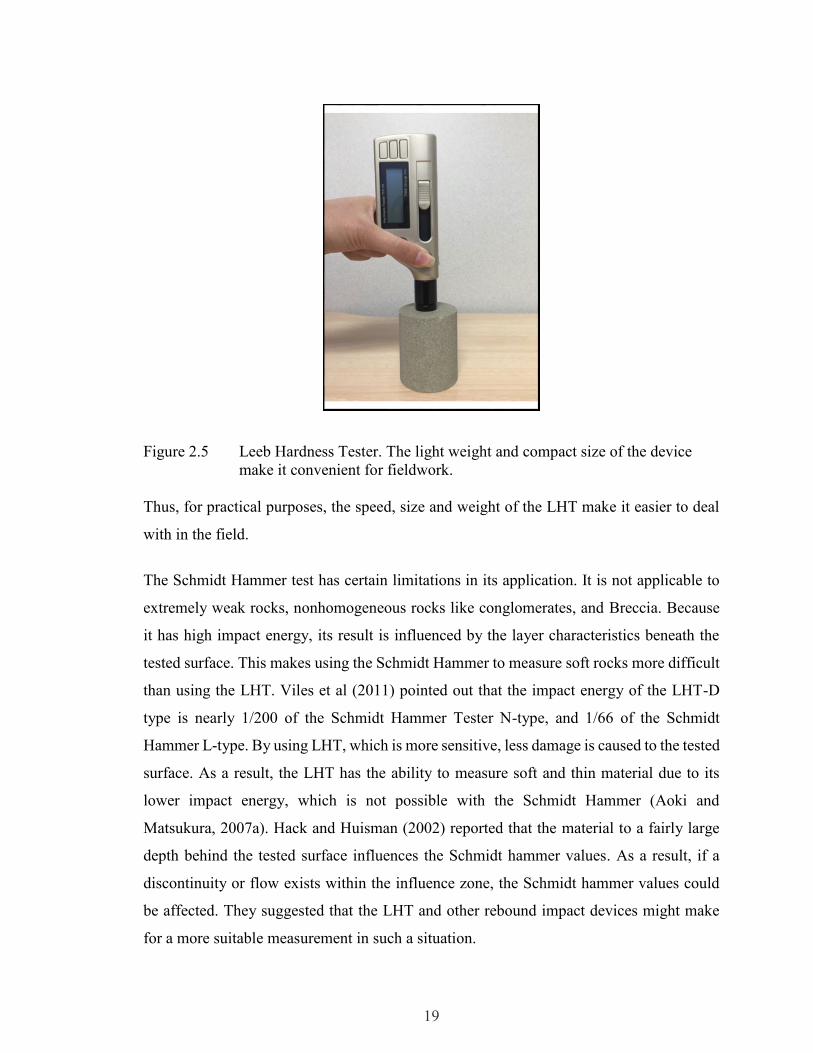
19
Figure 2.5 Leeb Hardness Tester. The light weight and compact size of the device
make it convenient for fieldwork.
Thus, for practical purposes, the speed, size and weight of the LHT make it easier to deal
with in the field.
The Schmidt Hammer test has certain limitations in its application. It is not applicable to
extremely weak rocks, nonhomogeneous rocks like conglomerates, and Breccia. Because
it has high impact energy, its result is influenced by the layer characteristics beneath the
tested surface. This makes using the Schmidt Hammer to measure soft rocks more difficult
than using the LHT. Viles et al (2011) pointed out that the impact energy of the LHT-D
type is nearly 1/200 of the Schmidt Hammer Tester N-type, and 1/66 of the Schmidt
Hammer L-type. By using LHT, which is more sensitive, less damage is caused to the tested
surface. As a result, the LHT has the ability to measure soft and thin material due to its
lower impact energy, which is not possible with the Schmidt Hammer (Aoki and
Matsukura, 2007a). Hack and Huisman (2002) reported that the material to a fairly large
depth behind the tested surface influences the Schmidt hammer values. As a result, if a
discontinuity or flow exists within the influence zone, the Schmidt hammer values could
be affected. They suggested that the LHT and other rebound impact devices might make
for a more suitable measurement in such a situation.

20
Furthermore, moisture can influence Schmidt Hammer test results, but does not
significantly influence the LHT readings. Aoki and Matsukura (2007) examined this by
preforming the tests on a sample when wet and when dry. Haramy and DeMarco (1985)
reported that the Schmidt hammer is affected by water content of the surface in addition to
the roughness of the surface area, rock strength, cleavage and pores as well. The LHT
device is sensitive to surface conditions, so it cannot be used successfully on friable or
rough surfaces of rocks.
The LHT has the ability to repeat the impact test on the same sample, and even on the same
spot without breaking the sample, which is not always possible with the Schmidt hammer
(Aoki and Matsukura, 2007a). This allows the LHT to be used on small specimens or on
those of limited thickness. In the laboratory, both devices require the specimens to be well
clamped in order to avoid any movement. The Schmidt hammer is less sensitive to
localized conditions at the impact location, making readings more consistent and
representative of the average rock properties. The LHT is more precise (i.e. covers a smaller
area), and therefore is affected by local mineralogy and geometry. Doing multiple Leeb
readings and averaging them for a single “test” reading can alleviate this pitfall. LHT has
certain advantages, such as the smaller diameter of its tip (3 mm), which allows for greater
accuracy of its measurement. Another advantage is the device’s automatic correction of the
angle (Yilmaz, 2012), which minimizes the variations in measurements produced by the
gravity force. In addition, the LHT can be used in either the laboratory or the field because
of its portability, simplicity, low cost, speed and non-destructiveness (as shown in Figure
2.6). Also, it positions at any angle on either a straight or curved surface, while the Schmidt
hammer’s direction is restricted.

21
Figure 2.6 Leeb hardness tester vs. Schmidt hammer
2.5 Previous Studies on Leeb Hardness Tester (LHT)
LHT has been used widely to estimate the rock UCS by several authors (Table 2.2).
Verwaal and Mulder (1993) at the Delft University of Technology examined the possibility
of predicting the UCS from HLD value. They reported results on a UCS versus HLD
relationship, as well as on the influence of the surface roughness on the LHT measurement.
They also observed that the sample thickness has slight effect on the LHT measurement.
They used limestone core specimens of three different types: 15 cm long with diameters of
3, 6, and 10 cm. The HLD values were taken as the average of ten radial impacts. It was
noticed that the hardness tests performed on 3 cm diameter cores provided HLD lower than
those of the 6 and 10 cm diameter. Consequently, it was concluded that the LHT may not
give appropriate hardness values with cores smaller than 5.4 cm in diameter. They ended
with a simple equation for estimating UCS from the measurements of LHT.
Additionally, Hack et al. (1993) used both LHT and ball rebound tests to describe the UCS
of the discontinuity plane for mixed lithologies of various rock type specimens. They
studied the effect of unit weight on the hardness values of both devices. They reported that
the results have an inverse relation. Furthermore, no relationship between Young's modulus
and hardness rebound values was found.

22
Table 2.2 Proposed correlation equations for UCS and Rebound hardness values
(RHN)
Source Leeb - UCS Equation R2 Tested
rock
Number
of
sample
Verwaal and
Mulder
(1993)
UCS= 8 X 10⁻⁶ RHN 2.5 0.77 mix 28
Meulenkamp
(1997)
UCS=1.21E-11 RHN3.8 - - -
Meulenkamp
and Grima
(1999)
UCS=0.25RHN+28.14density-
.75porosity-15.47grainsize-
21.55rocktype
- mix 194
Grima and
Babuska
(1999)
UCS=0.386RHN+39.268Density-
1.307Porosity- 246.804
- mix 226
Meulenkamp
and Grima
(1999)
UCS=1.75 E-9 RHN 3.8 0.806 mix 194
Verwaal and
Mulder
(2000)
UCS= 3.38E-9 RHN 2.974 - mix 28
Kawasaki et
al (2002)
UCS=1.49+0.248RHN 0.578 sandstone 5
Kawasaki et
al (2002)
UCS=64.6+0.122RHN 0.339 hornfels 5
Kawasaki et
al (2002)
UCS=156+0.309RHN 0.818 shale 11
Kawasaki et
al (2002)
UCS=271-0.38RHN 0.356 granite 3
Kawasaki et
al (2002)
UCS=538+0.939 RHN 0.811 sandstone 8
Aoki and
Matsukura
(2008)
UCS= 0.079 e -0.039 n RHN 1.1 0.88 mix
Yilmaz
(2013)
UCS= 4.5847 ESH-142.22 0.674 carbonate 18
Lee et al
(2014)
UCS= 2.3007 e 0.0057RHN 0.8235 shale 24
23
Source Leeb - UCS Equation R2 Tested
rock
Number
of
sample
Lee et al
(2014)
UCS= 2.1454 e 0.0058 RHN 0.8093. shale 24
Lee et al
(2014)
UCS= 3.7727 e 0.005 RHN 0.7799 shale 24
* Equotip Shore hardness (ESH), RHN= rebound hardness number (Equotip)
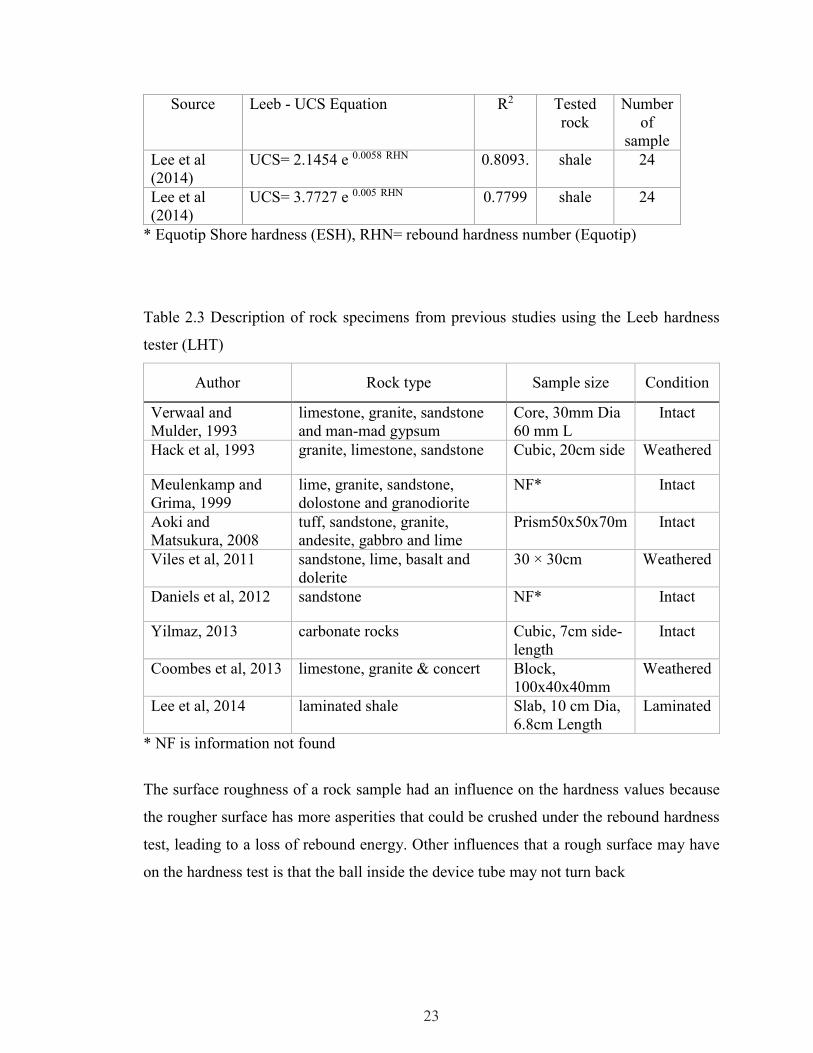
Table 2.3 Description of rock specimens from previous studies using the Leeb hardness
tester (LHT)
Author Rock type Sample size Condition
Verwaal and
Mulder, 1993
limestone, granite, sandstone
and man-mad gypsum
Core, 30mm Dia
60 mm L
Intact
Hack et al, 1993 granite, limestone, sandstone Cubic, 20cm side Weathered
Meulenkamp and
Grima, 1999
lime, granite, sandstone,
dolostone and granodiorite
NF* Intact
Aoki and
Matsukura, 2008
tuff, sandstone, granite,
andesite, gabbro and lime
Prism50x50x70m Intact
Viles et al, 2011 sandstone, lime, basalt and
dolerite
30 × 30cm Weathered
Daniels et al, 2012 sandstone NF* Intact
Yilmaz, 2013 carbonate rocks Cubic, 7cm side-
length
Intact
Coombes et al, 2013 limestone, granite & concert Block,
100x40x40mm
Weathered
Lee et al, 2014 laminated shale Slab, 10 cm Dia,
6.8cm Length
Laminated
* NF is information not found
The surface roughness of a rock sample had an influence on the hardness values because
the rougher surface has more asperities that could be crushed under the rebound hardness
test, leading to a loss of rebound energy. Other influences that a rough surface may have
on the hardness test is that the ball inside the device tube may not turn back
24
perpendicularly and could touch the tube sides (friction), resulting in the reduced height of
the ball rebound. Therefore, they suggested that, before conducting the rebound hardness
testing, the surface should be reasonably smooth – e.g. simple grinding and sawing
processes are satisfactory enough to get a smooth surface. Furthermore, the hardness values
are affected more by the asperity crushing and sample surface in the case of soft rocks. In
the case of the hard rocks, the hardness values are affected more by the parameters of
elasticity. Hack and colleagues (1993) attempted to uncover a relationship between the
UCS and the rebound value, to estimate the mechanical strength of the rock surface along
a discontinuity using the Verwaal and Mulder equation.
Asef (1994) used 55 block specimens from 14 different rock types, mostly sedimentary. He
attempted to develop an empirical method relating UCS, Young’s modulus and LHT by
using three (3) types of Equotip (D with ball, D without ball, and C). He reported that
dryness, density, surface roughness and size, and impact body and shape affected the
Equotip values. He used different impact methods; for example, one such method is where
10 impacts on different spots are measured (the results present a stronger correlation). He
applied the same method on untreated smooth surfaces of block specimens. He used a 40
mm core diameter for strong rocks and 50 mm for weak rocks. He used the
STRATGRAPHICS software to calculate S, and V for LHT values. The results for
uniform rocks show a low , and anisotropic specimens with irregular roughness had the
highest variation. Linear, multiplicative and exponential correlations were reported; the
multiplicative results displayed strongest correlation. Asef (1994) concluded that the values
of Leeb that had not been processed for highest and lowest readings showed the highest
variance.
In the following year, Asef (1995) studied four types of rocks (very strong, strong, weak
and very weak). For stronger rocks the HLD values show no significant change related to
the length of specimens, however, for medium to weak rocks his study reports that the size
of specimens can influence the Leeb values, the LHT values are decreased with the decrease
in the sample size, the sample length should be at least 6-9 cm long to avoid the size effect,
and the higher strength values of rock specimens tend to be more scattered.
25
Meulenkamp and Grima (1999) used a neural network to predict the UCS from HLD and
several other rock characteristics (porosity, density, grain size and rock type) as input.
However, this is a complex approach and required many input parameters, each of which
added complexity and additional uncertainty to the method. This removed the “simplicity”
of the test and it restricted their approach to the availability and quality of the secondary
inputs. Moreover, the proposed equation includes many variables, which in turn is not
practical in field estimation. Finally, to the author’s knowledge, the neural network
algorithm details were not published and made readily available.
Okawa et al. (1999) tested the effects of the measurement conditions on the rebound value
and concluded that the rebound value depends partially on specimen support (i.e., physical
constraint). In addition, multiple tests on the exact same location tend to increase the local
density, thus HLD increases with additional impacts at a given point. The roughness of the
testing surface has no clear influence on the test result of rebound value.
Kawasaki and colleagues (2002), studying unweathered rocks, proposed that the UCS could
be estimated from LHT values by using the Leeb test to establish the strength of rocks in
the field. They also established the effects of the test conditions, including the roughness
and size of the sample and the impact direction, and used cylindrical specimens of rock
types including sandstone, shale, granite, hornfels and schist, collected from different
locations in Japan. They reported that the specimen thickness has slight influence on the
LHT measurement in specimens more than 50 mm thick. In 2007, Aoki and Matsukura
used the type “D” hardness tester to study rock hardness from nine
locations, eight in Japan and one in Indonesia. They proposed an equation relating UCS to
HLD and porosity:
𝑈𝐶𝑆 = 0.079𝑒−0.039𝑛 𝐻𝐿𝐷1.1 [2-10]
Where “n” is the porosity and “HLD” is the Leeb hardness value.
26
The LHT has been used to study the degree of weathering. Aoki and Matsukura (2008)
investigated the degree of weathering by examining the difference between the repeated
impact method and the single impact method. Another specific weathering assessment of
the LHT in terms of rock surfaces is when Viles et al. (2011) compared mean hardness
values at fifteen different sites determined by four testing devices including Equotip,
piccolo, silver Schmidt (silvers) and classic Schmidt (classics). They studied their hardness
before and after applying carborundum to see the impact of carborundum pretreatment on
the results. Moreover, they conducted comparisons for all four devices divided by the rocks
having differences in wetness/dryness of its surface area, surface hardness, boulder size
influence, edge effects, and operator variance. They concluded that each device has its
strengths and weaknesses depending on the purpose of collecting the hardness values. The
LHT has been shown in their study to be insensitive to block size for the range of sizes in
their study. They studied the sample size effect on the HLD values, on sandstone block
from Oribi Vulture site that have volumes that ranged between under 200 cm3 to nearly
20000 cm3 and 30 hardness values were taken with the Equotip device. They concluded
that there is no relationship between the sample size and the HLD values.
More recently, Daniels et al. (2012) studied the strength of sandstone. They indicated that
the original Verwaal and Mulder (1993) correlation could overestimate the rock strength of
weak sandstone. Yilmaz (2013) considered only one rock group (carbonate rocks) to
determine the suitability of different rebound testing procedures with the LHT for UCS
estimations and came up with different regression models. He used a new testing
methodology, hybrid dynamic hardness (HDH), which depends on a combination of the
surface rebound hardness and compaction ratio (the ratio between HLD and the peak
hardness value earned after ten repeated impacts at the same spot) of a rock material. He
pointed out that the predicted UCS is more accurate when density is available, which means
that density is also could be correlated to intact strength. Moreover, he reported that there
is no clear evidence of size effect on the hardness values. He experimentally studied the
effect of sample size on the HLD values by using the EHT on 18 different types of rock
specimens. Cubic specimens with 7 cm sides were tested

27
combined with other cubic specimens with 5, 9, 11, 13, and 15 cm sides. All specimens
were grounded with 220 sand paper and dried for 24 hours. The hardness tests were
performed with 20 single impacts and then got averaged. He attributed the variations in the
HLD values to the in-homogeneities existing in the fabric of rock, rather than the size of
the specimen and the dissipation of impact energy to “the randomly distributed voids
underneath the tested surfaces” (Yilmaz, 2013). He recommended that there is a need for
more studies on other rock types with different geometries to investigate the sample size
effect.
In the case of layered rocks, Lee et al. (2014) applied LHT in order to estimate the UCS of
laminated shale formations. They updated the calibration equation using 62 points from
Meulenkamp (1997), Meulenkamp and Grima (1999) and Verwaal and Mulder (2000). In
addition, Lee et al. (2014) investigated the effect of sample thickness by studying
relationship between density and thickness on a reference test block (a dense material of
steel with a dimension of 9.14 cm in diameter and 5.84 cm in thickness). The measurements
were taken using the Equotip Hardness Tester. The HLD measured from the block is
consistent since it is an isotropic and homogeneous continuum material. Lee and colleagues
(2014) used aluminum (Al) 6061-T6 specimens to examine the effect of sample length on
HLD with specimens that have identical density (2.70 g/cm3). Their Al specimens have
exactly the same diameter of 3.81 cm and six different lengths as following 2.54, 5.08, 7.62,
10.16, 12.7, and 15.24 cm, respectively. They found that the HLD increases as sample
length increases, until the tested material reaches a minimum length to obtain consistent
HLD. It is noted that the HLD of the
specimens increased in a non-linear form until 12.7 cm. The study proposed that this value
is the minimum length of the Al sample for valid measurement of HLD based on its density.
The study also examined the thickness effect of shale cores with 10.16 cm in diameter for
both sections: 3.38 cm slab and 6.78 cm of butt sections. For each core section, the impact
direction is perpendicular to the cut face. The measurements were repeated at the same
depth, but on different spots on the sample. For each depth, the mean

28
value was recorded. It was concluded that the HLD of the 2/3 butt section is higher than
the 1/3 slab section.
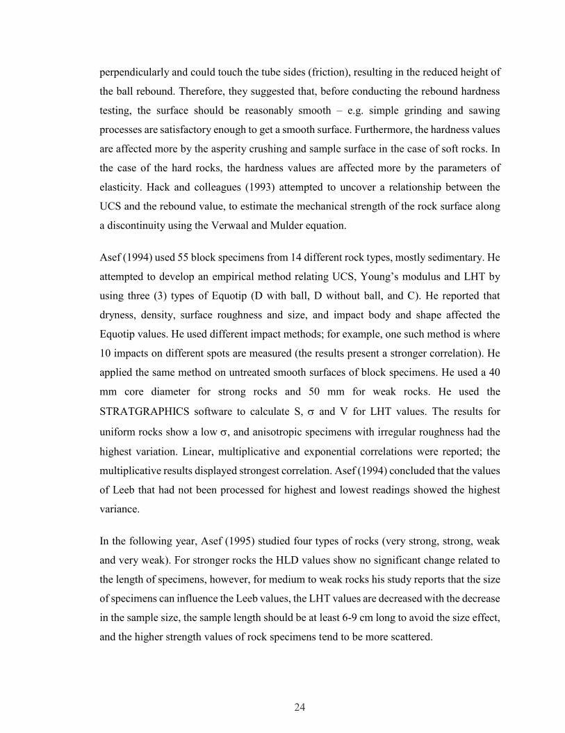
Figure 2.7 shows the HLD and UCS proposed correlations of previous studies that were
conducted using LHT. Some proposed correlations were selected over others because some
papers imbedded their datapoints inside other paper's curve, e.g. Lee at al (2014), and Aoki
and Matsukura (2007) used the correlation curve of Verwaal and Mulder (1993).
Figure 2.7 HLD and UCS proposed correlation of previous studies (Verwaal & Mulder,
1993; Asef, 1995; Aoki & Matsukura, 2007; Meulenkamp & Grima, 1999)
0
100
200
300
0 200 400 600 800 1000
UC
S (
MP
a)
HLD
Aoki and
Matsukura, 2007
Meulenkamp and
Grima, 1999
Asef, M, 1995
Verwaal and
Mulder, 1993
Aoki &
Matsukura, 2007
Meulenkamp &
Grima, 1999
Asef,M, 1995
Verwaal &
Mulder, 1993
29
CHAPTER 3 STUDY METHODOLOGY
This chapter describes the test methodology that has been used to achieve the main goal of
this study, which is to develop a relationship between UCS and HLD values. The chapter
begins by discussing lab testing methodology which includes collecting, UCS tests on
specimens, how they were prepared based on the ASTM recommendations, and LHT on
core and cubic specimens. Following that is a discussion of analysis methods, which
includes an evaluation of Leeb test methodology. Two methods have been used to evaluate
the LHT: the first is to evaluate the number of impacts, and the second is to evaluate the
sample size. The final section in this chapter is Leeb – UCS correlation. Statistical analysis
(Regression, T-Test, F-Test, residual) has been used to develop the relationship between
the mean value of hardness tests and their corresponding rock strengths.
This study used LHT (“D” type) series TH170, to measure the non-destructive hardness
values of rock specimens to relate them to the UCS values to investigate and develop an
appropriate relationship between the two mechanical properties of rock specimens. The
TH170 accuracy varies with respect to different testers and scales of hardness; however, it
is able to compare and convert these values into several types of hardness, and the accuracy
of measuring was commonly taken as ±0.5% (see the instruction manual of the TH 170).
The LHT is a portable hardness tester developed for measuring the hardness of rock
materials. It is very convenient and easy to use in the laboratory as well as in the field. This
was the first stage in developing a robust relationship linking HLD to UCS, which is
described in the subsequent chapters of this study. The manufacturer’s manual specified
that the minimum weight of the test piece should be 0.05-2 kg and the roughness of the
surface equal to or less than 1.6 micrometer for accurate hardness test results and the testing
method described in this chapter confirmed all these recommendations.
30
3.1 Lab Testing Methodology
This section contains a discussion of the lab test methodology which was used in this
research. Included in this section are the locations the specimens were taken from, how
they were collected, and the number of specimens obtained. This section also includes a
discussion of the UCS test methodology used in the study, including sample preparation.
Finally, LHT testing methodology for core and cubic specimens is discussed.
3.1.1 Collection
In this study, significant laboratory work was carried out in cooperation with other
researchers on collected specimens from the mining industry partners and from local
quarries. Therefore, the database was obtained from diverse sources; university lab
specimens were combined with other literature to build a database with a total of 336 points
to use in this research. The specimens that were obtained for the test results in our lab
originate in diverse Quarries throughout Nova Scotia.
3.1.1.1 Previously Published
There are two methods used to obtain from previously published work. The first method is
to obtain them directly from the published tables. The second way is to digitize them from
an image of a graph that presents the points. The first way to get from the tables is a direct
way, but it is impossible to obtain the existing on the image of the graph without using a
special software that has the ability to pick the values of those on the image of the graphs.
For that reason, ‘Graph Click’ software was used as a graph digitizer software, which
allows researchers to automatically regain the original (x, y) from the graphs. In other
words, if one has a graph as an image, but not the corresponding, the only way to get the
trajectory of a graph is the graph digitizer software or by hand. Graph Click is one of the
best ways to deal with that kind of issue. By clicking on the image of the plot, the obtained
coordinates of the points can be directly exported into Microsoft Excel or any other similar
31
application. This software has many features including image modification, an unlimited
undo function, handling with two ordinate axes, covering for different scales such as linear,
logarithmic or inverse scales, and the use of several sets in the same document.
3.1.1.2 Quarries
A number of the points that were used in this study were collected from the test results on
specimens brought in May 2015 from quarries located in Nova Scotia. Sandstone rocks
with intruding organic matter dots and classic olive grey colour were collected from
Wallace Quarries Ltd, which is located at Wallace, Nova Scotia, Canada. The site is
approximately 163 km from Halifax, Nova Scotia, Canada. Wallace sandstone is known as
one of the most durable sandstones in the world and it has been quarried for the last 150
years.
Dolostone blocks were brought from Halifax Stone LTD, Middle Musquodoboit, NS,
Canada. The site is approximately 67 km from Halifax, NS, Canada. The weathered porous
limestone blocks were brought from Mosher Limestone Company LTD, Upper
Musquodoboit, NS. The site is approximately 90 km from Halifax, NS, Canada.
Schist rocks were brought from a mine in eastern Canada: three Quartz Sericite Schist core
specimens, (two of them show a foliation of 45 to the core axis and one has a 40 foliation
to the core axis), five Quartz Chlorite Schist core specimens, (two with a foliation angle of
45 to the core axis, two with a 40 angle, and one with a 30 angle) and two core specimens
of Mafic Dyke. The mine is located in Newfoundland. The site is approximately 1000 km
from Halifax, NS. All schist rocks (soft rock) are foliated and host stringer pyrite. Some of
the foliated schist core specimens are damaged a bit from blasting and have natural
fractures.
Coal Sandstone (a micro defected gray sandstone with coal bands) was obtained from the
Stellarton Surface Coal Mine, which is an open pit coal mine located at 1 Westville, Nova

32
Scotia, Canada. It is owned and operated by Pioneer Coal Limited. The site is
approximately 150 km from Halifax, NS, Canada. Greywacke is from the Lower
Ordovician Meguma Group. Slate (Metamorphic Rock), which is formed when fine-
grained sedimentary rock (shale) is exposed to high pressure deep beneath the surface of
the earth, is characterized by the way it breaks, along closely spaced parallel fractures (U.S.
Geological Survey). A granite block, 35 cm x 25 cm x 15 cm, approximately, was picked
up from Langes Rock Farm Ltd, Maplewood, Nova Scotia. The site is approximately 120
km from Halifax, NS, Canada.
Within the framework of this study, rock blocks were cored and inspected for the existence
of any macro-defects so that standard specimens with no cracks and fractures would be
used. It is well known that porosity and anisotropy (schistosity and foliation) are the
mechanical parameters affecting the mechanical properties (HLD, UCS, etc.) of the rock
specimens. This study attempted to avoid the effecting of these parameters by picking the
specimens that show no high porosity and performing the tests with considering of foliation
plans.
All specimens were marked, labeled, and the specimen geometry was checked prior to the
lab tests to minimize any error during the experiments. For the UCS tests and hardness
tests, the specimens were labeled as the following (S.S) for sandstone (C) for Coal (mine)
sandstone, (L) for limestone, (D) for dolostone, (G) for granite, (W) for greywacke, (SH)
for schist with horizontal foliation to axial load, (SV) for schist with vertical foliation to
axial load.

33
(a) Schist (b) Dolostone
(c) Greywacke (d) Granite
(e) Wallace Sandstone (f) Granite
Figure 3.1 (a, b, c, d, e and f) Block specimens of various rock types that were used in
this study from mining operations Eastern Canada.
3.1.2 UCS Testing
In this study, our core specimens, with 54 mm diameter and 113 - 121 mm height, were
prepared from a block from different rock types (granite, schist, limestone, marble,
dolostone and sandstone), which were obtained from different mining operations in Eastern
Canada (see quarries section). All UCS tests were carried out in the Dalhousie University
laboratory, Halifax, Nova Scotia, Canada. In this study, the core specimens were prepared
for the UCS tests, and are as follows: three Quartz Sericite Schist, two of which show
foliation of 45 to core axis and one with 40 to core axis; 5 Quartz Chlorite

34
Schist, two with a foliation angle of 45 to the core axis, and the other two with a 40 angle,
and one with a 30 angle, and 2 core specimens of Mafic Dyke. In addition, two sandstone
core specimens, three limestone core specimens, three Greywacke core specimens, three
dolostone core specimens, four Granite core specimens, 12 Schist core specimens with
horizontal foliation, sex Schist core specimens with vertical foliation, three Coal sandstone
core specimens, and 6 Slate core specimens (Metamorphic Rock) were used. Four months,
from May 2015- August 2015, were spent on UCS tests, from the first day the specimens
arrived at our lab until we finished all UCS tests. Table 3 provides details of the used core
specimens.
Table 3 The core specimens that were prepared for the UCS tests in present study
Number of sample Lithology Foliation to core axis
3 quartz sericite schist 1-> 40°;2-> 45°
5 quartz chlorite schist 1-> 30°;2-> 40°;2-> 45°
2 mafic dyke unfoliated
2 sandstone unfoliated
3 limestone unfoliated
3 greywacke unfoliated
3 dolostone unfoliated
4 granite unfoliated
12 schist 90°
6 schist 0°
3 coal sandstone 90°
After that, a compression-testing machine of about 2000 kN (200-tonne) capacity with a
loading rate of 0.3 - 0.5 mm/min was applied for UCS tests with a duration of 7 – 13 minutes
in average (see section 2.1.1)
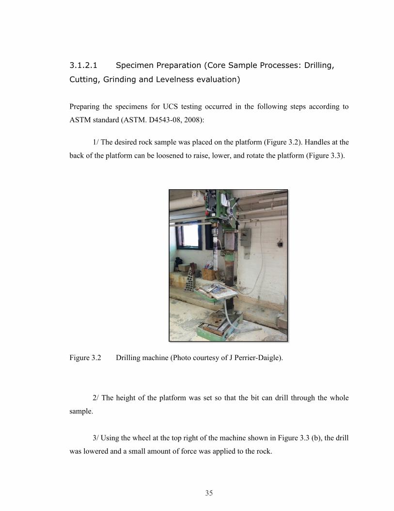
35
3.1.2.1 Specimen Preparation (Core Sample Processes: Drilling,
Cutting, Grinding and Levelness evaluation)
Preparing the specimens for UCS testing occurred in the following steps according to
ASTM standard (ASTM. D4543-08, 2008):
1/ The desired rock sample was placed on the platform (Figure 3.2). Handles at the
back of the platform can be loosened to raise, lower, and rotate the platform (Figure 3.3).
Figure 3.2 Drilling machine (Photo courtesy of J Perrier-Daigle).
2/ The height of the platform was set so that the bit can drill through the whole
sample.
3/ Using the wheel at the top right of the machine shown in Figure 3.3 (b), the drill
was lowered and a small amount of force was applied to the rock.

36
(a) (b)
Figure 3.3 Close up of drill platform (a) and drill handles (b) (Photo courtesy of J
Perrier-Daigle).
4/ The drill bit was lifted off the rock, and the green button was pushed to start the
drill.
5/ The water valve was partially opened, and drilling manually, the drill was slowly
lowered into the rock sample. Applying very little force, a pilot hole was drilled into the
rock approximately ¾ of the drill bit tip deep.
6/ After the pilot hole was drilled and the drill bit was determined to not shake, the
gray lever was pushed to activate the automatic feeder, and then the water valve was fully
opened.
7/ The drill was monitored regularly to make sure that the bit was not shaking and
the rock was stable. Once the drill bit reached the end of the rock sample, the drill was
turned off.
Some rock types were relatively weak, and fractured during drilling, leaving unusable core
specimens. These rocks were examined for discontinuities, fractures, or joints in the rock.
Furthermore, some rocks had dominant structural orientations such as schist, and it is

37
necessary to make sure that one is drilling in the proper orientation, avoiding any fractures
in the rock specimen that may result in cracked or weakened specimens.
Care was taken during drilling near the edge of a rock or next to another drill hole. Drilling
a hole approximately 1 cm away from another hole may cause the drill to tear the supporting
wall between the two holes.
Figure 3.4 Blade rock saw machine (Photo courtesy of J Perrier-Daigle).
In the cutting stage, after drilling the sample, the core still had rough ends. These ends cut
in order to test the specimens with an even load distribution. Since the rock needed to be
cut, this was done with the wet blade saw machine shown in Figure 3.4. The machine uses
a diamond-encrusted blade that moves at a set rate while constantly being lubricated.

38
Figure 3.5. Close up of vice controls inside the wet blade saw machine ("Photo courtesy
of J Perrier-Daigle).
The core was placed in the vice, and another sample was placed beside core specimens that
were shorter than the length of the vice to prevent any vibrations while cutting. The vice
was tightened using the knob shown in the center of Figure 3.5. Using the wheel on the
right, the vice slid, allowing the blade to cut the sample to the desired length, and the top
hatch of the machine was lowered when the sample was ready.
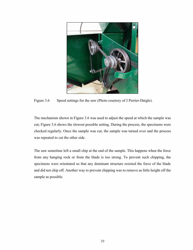
39
Figure 3.6 Speed settings for the saw (Photo courtesy of J Perrier-Daigle).
The mechanism shown in Figure 3.6 was used to adjust the speed at which the sample was
cut; Figure 3.6 shows the slowest possible setting. During the process, the specimens were
checked regularly. Once the sample was cut, the sample was turned over and the process
was repeated to cut the other side.
The saw sometime left a small chip at the end of the sample. This happens when the force
from any hanging rock or from the blade is too strong. To prevent such chipping, the
specimens were orientated so that any dominant structure resisted the force of the blade
and did not chip off. Another way to prevent chipping was to remove as little height off the
sample as possible.
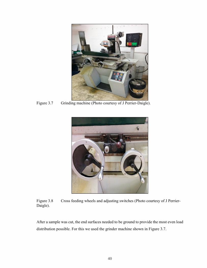
40
Figure 3.7 Grinding machine (Photo courtesy of J Perrier-Daigle).
Figure 3.8 Cross feeding wheels and adjusting switches (Photo courtesy of J Perrier-
Daigle).
After a sample was cut, the end surfaces needed to be ground to provide the most even load
distribution possible. For this we used the grinder machine shown in Figure 3.7.
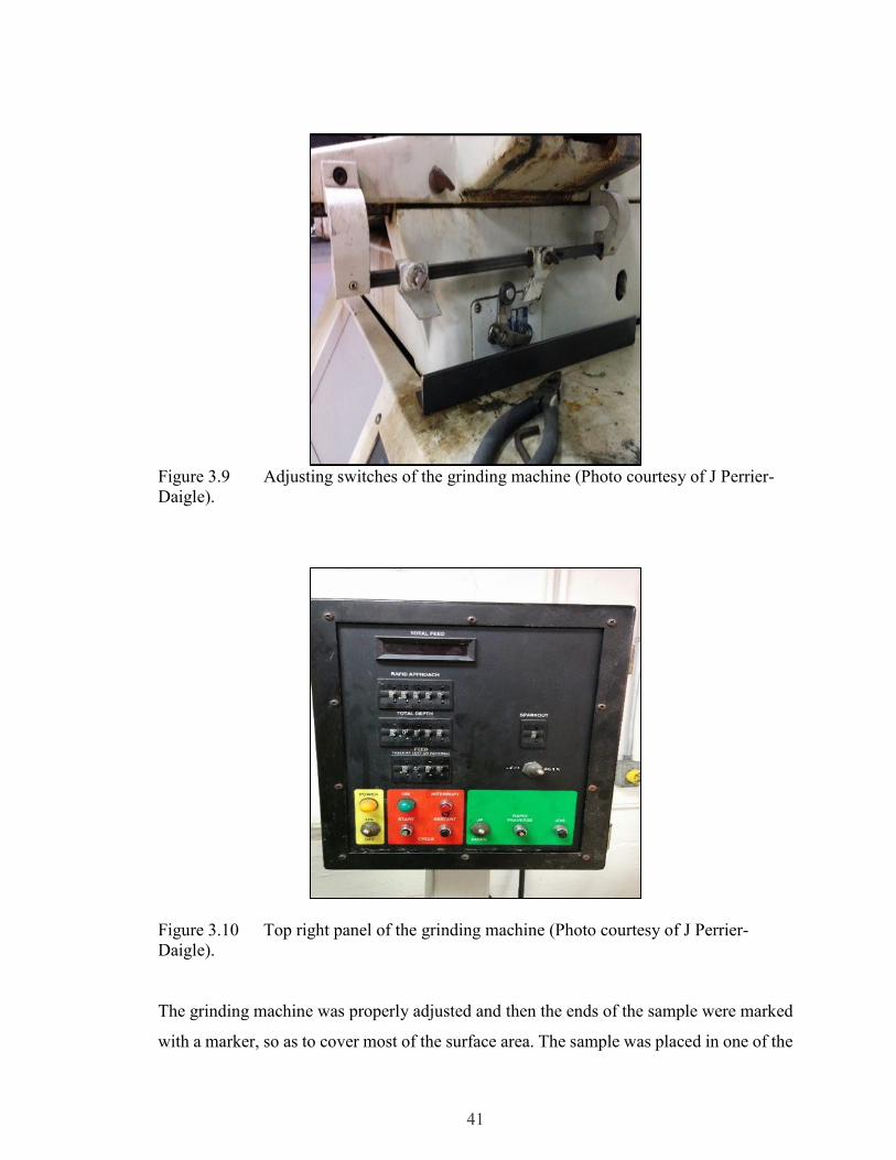
41
Figure 3.9 Adjusting switches of the grinding machine (Photo courtesy of J Perrier-
Daigle).
Figure 3.10 Top right panel of the grinding machine (Photo courtesy of J Perrier-
Daigle).
The grinding machine was properly adjusted and then the ends of the sample were marked
with a marker, so as to cover most of the surface area. The sample was placed in one of the
42
four slots of the v-clamp. Figures 3.8 and 3.9 show the grinding switches that adjusted the
area that was ground. Once the spindle was set at the appropriate height and was not
touching the sample, the grinding began. The top right panel was turned on (Figure 3.10),
the increment (in inches) was selected, and then, by adjusting its keys, the grinder started
to descend. This should generally be around 13 µm.
3.1.2.2 UCS Test Preparation
The following are the steps followed in preparation for performing UCS testing on the
specimens:
Step 1: Sanding
Sanding the specimens creates a relatively flat surface so the strain gauge can rest evenly
on each sample. Sanding likewise provides a smoother area for the gauge to bond to.
Step 2: Strain gauges’ application
The second step of preparing a core for UCS testing is to apply strain gauges to some of
the specimens; this is the most sensitive part of the UCS test preparation.
3.1.2.3 Specimen Specification
After the previous steps, the core sample was ready for testing. Several vital pieces of
information were noted before breaking the specimens for the UCS test. It is necessary to
have information such as such as the height, diameter, weight, etc. of the sample written
down before it is broken. Before performing the UCS test, each sample was examined
thoroughly for any dominant structures, flaws, or inclusions, and the observations were
written down and photographed; pictures were also taken of each core sample before and
after testing.
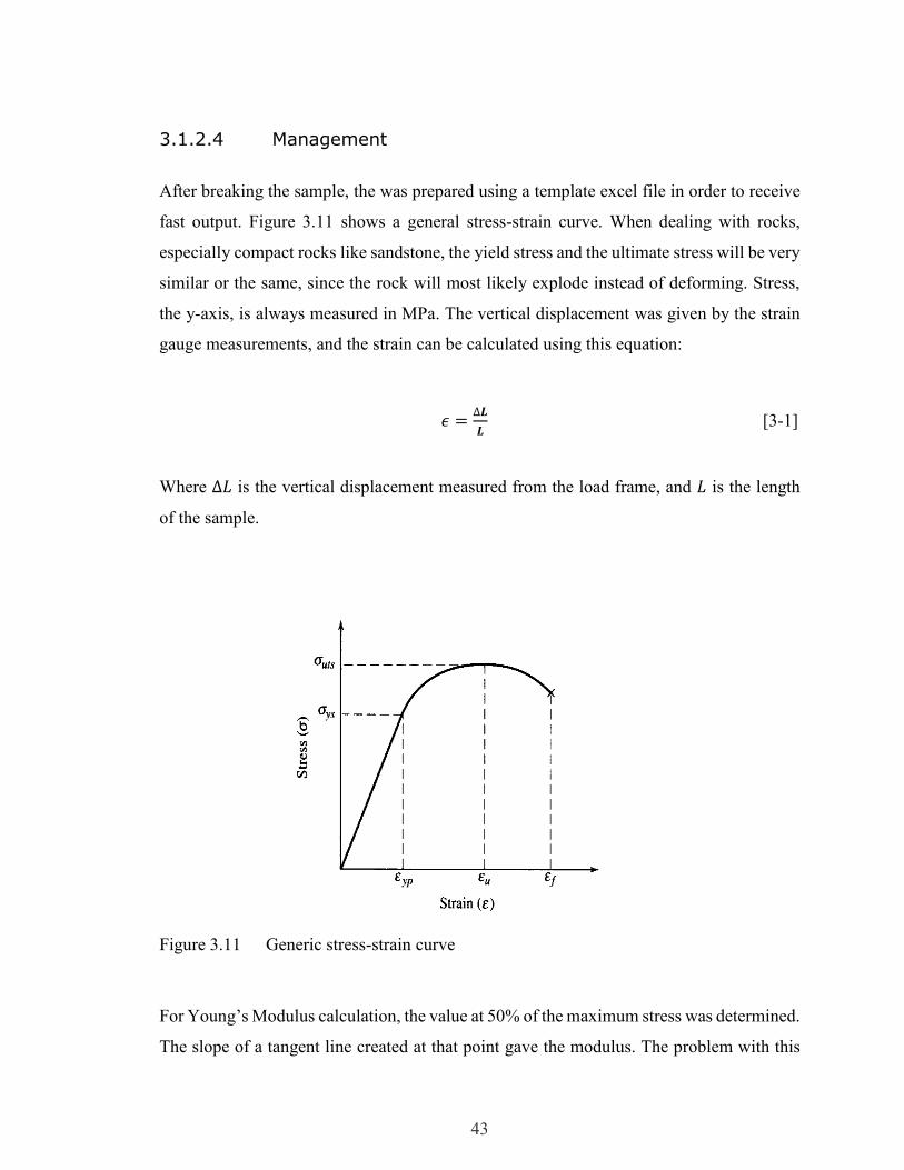
43
3.1.2.4 Management
After breaking the sample, the was prepared using a template excel file in order to receive
fast output. Figure 3.11 shows a general stress-strain curve. When dealing with rocks,
especially compact rocks like sandstone, the yield stress and the ultimate stress will be very
similar or the same, since the rock will most likely explode instead of deforming. Stress,
the y-axis, is always measured in MPa. The vertical displacement was given by the strain
gauge measurements, and the strain can be calculated using this equation:
𝜖 =∆𝑳
𝑳 [3-1]
Where ∆𝐿 is the vertical displacement measured from the load frame, and 𝐿 is the length
of the sample.
Figure 3.11 Generic stress-strain curve
For Young’s Modulus calculation, the value at 50% of the maximum stress was determined.
The slope of a tangent line created at that point gave the modulus. The problem with this

44
method was that there were many points off, which created a zigzag pattern, and calculating
the modulus from one single point would give an inaccurate value. Instead, a more practical
way of calculating Young’s Modulus is to select several points of around the point, and
create a linear line of best fit to find its slope. If there is a discontinuity in the at half its
maximum stress, such as a major dip in stress levels, another point was chosen - above the
half point - where there is a linear section of. Young’s Modulus has units of GPa, and that
strain was measured in % on the graph.
In order to calculate the Modulus Ratio, the following equation was used:
𝑀𝑅 = 𝐸/𝜎𝑐, [3-3]
Where 𝐸 is the Young’s Modulus, and 𝜎𝑐 is the ultimate compressive stress.
Figure 3.12 UCS test machine with a sandstone sample.
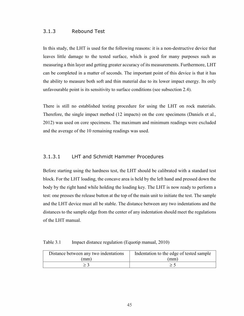
45
3.1.3 Rebound Test
In this study, the LHT is used for the following reasons: it is a non-destructive device that
leaves little damage to the tested surface, which is good for many purposes such as
measuring a thin layer and getting greater accuracy of its measurements. Furthermore, LHT
can be completed in a matter of seconds. The important point of this device is that it has
the ability to measure both soft and thin material due to its lower impact energy. Its only
unfavourable point is its sensitivity to surface conditions (see subsection 2.4).
There is still no established testing procedure for using the LHT on rock materials.
Therefore, the single impact method (12 impacts) on the core specimens (Daniels et al.,
2012) was used on core specimens. The maximum and minimum readings were excluded
and the average of the 10 remaining readings was used.
3.1.3.1 LHT and Schmidt Hammer Procedures
Before starting using the hardness test, the LHT should be calibrated with a standard test
block. For the LHT loading, the concave area is held by the left hand and pressed down the
body by the right hand while holding the loading key. The LHT is now ready to perform a
test: one presses the release button at the top of the main unit to initiate the test. The sample
and the LHT device must all be stable. The distance between any two indentations and the
distances to the sample edge from the center of any indentation should meet the regulations
of the LHT manual.
Table 3.1 Impact distance regulation (Equotip manual, 2010)
Distance between any two indentations
(mm)
Indentation to the edge of tested sample
(mm)
3 5
46
In this study, the most popular standard was chosen for the Schmidt Hammer application
which is the American Society for Testing and Materials (ASTM). Applying 20 reading
impacts on our lab sandstone specimens for a comparison purpose with LHT. USING the
N-type of Schmidt Hammer that performs an impact energy of 2.207Nm. Discarding the
Schmidt numbers that differing more than seven units from the average. And then averaged
the remaining numbers. ASTM standard requires impacts be separated, to avoid overlap
data, at least one plunger diameter. The ASTM Standard (D5731-95) was performed for
application of Schmidt hammer. “The hammer was held vertically downward at right angles
to the horizontal rock surface” (Selçuka & Yabalaka, 2014). The core specimen surfaces
were smoothed to avoid an impact energy loss. 20 single readings were taken to obtain the
average Schmidt number
3.1.3.2 Core Specimen
In this study, the LHT was performed to link the HLD to the UCS results for our core
specimens. For that reason, the core specimens were prepared from different rock types
(see sample preparation section). There is still no established testing procedure for using
the LHT to predict UCS on rocks; therefore, the single impact method (12 impacts)
described above was used, and the results are presented in the next chapter.
Additionally, this study investigated and quantified the optimum readings (impacts) that
are required to get a valid LHT (see Number of Test section). Moreover, this study aims to
examine the relationship between the sample size and the mean HLD to investigate the
sample size effects (see Evaluation of Leeb Test Methodology section). For that reason, a
number of core sandstone specimens were prepared, followed by an experimental study
that was conducted on different sandstone sizes. All core specimens have been prepared
with the same diameter of 54 mm (NX-size) with eight different lengths. For each length,
the specimens were tested by the LHT, and the different core sample lengths after
preparation were 9, 10, 22, 38, 76, 102, 152, and 190.5 mm, respectively.

47
3.1.3.3 Cubic Specimen
In this study, the LHT (“D” type) was used to examine the relationship between the sample
size and the mean value of LH of cubic rock specimens. For that reason, the cubic
specimens were prepared from different rock types. The averaged LH readings were plotted
against the cubic sizes of rock specimens. Also, in this study, several cubic sandstone
specimens were prepared (refer to the sample size section). Four cubic specimens with
different lengths were prepared. For each length, the specimens were tested by the hardness
tester. The different four cubic sample lengths after preparation were 25, 51, 102, and 203
mm, respectively.
3.2 Analysis Methods
This section discusses the various methods used to analyze the retrieved from the testing
described above. Analysis and discussion of the results are covered in Chapter five.
3.2.1 Evaluation of Leeb Test Methodology
The appropriate number of impacts that are required to get a reasonable measure of the
“Statistically representative” hardness of the sample rock, given the sensitivity to localized
conditions, is a controversial issue amongst researchers. In order to address this issue and
quantify the appropriate readings (impacts), this study was carried out using two
approaches. First, an evaluation based on statistical theory was carried out, and, secondly,
an evaluation based on sampling was carried out. Also, the scale effect on the specimen
hardness has been addressed.
3.2.1.1 Number of Impacts Comprises a Test
As stated above, there were two types of tests carried out to quantify the appropriate number
of impacts. The first approach in this study used a core sample (sandstone, granite,
48
dolostone and schist) of a L/D ratio of 2-2.5 with a total length of 121 mm. The average of
100 repeat measurements (readings) on different pots of the core sample is considered as
the population mean (μ). The statistical measures of 100 readings on the core specimens,
including the μ and , are presented in next chapter in Table 4.1. After that, the margin of
error (𝑴𝑬) formula was used to determine the difference between the observed �̅� and the
μ when the experiment was repeated with the same testing condition for different sample
sizes (e.g. 10 and 15). This method aids in finding out how many impacts one would need
to get a �̅� which is almost equal to the μ, based on 100 readings with a degree of confidence
interval of 95%. The ideal sample mean can be quantified for sample sizes less than 100 by
using ME. The relation between the μ and �̅� can calculated using the following equation:
𝝁 = �̅� ± 𝟏. 𝟗𝟔 (𝝈
√𝒏 ) [4 -
1]
Where μ is the population mean, 1.96 is the critical Z value of the standard normal
distribution at a 95% degree of confidence, σ is the standard deviation of the population, n
is the sample size, and �̅� is the sample mean. The formula to establish the 𝑴𝑬 at different
sample sizes (e.g. at 10 and 15) is:
𝑴𝑬 = 𝟏. 𝟗𝟔 (𝝈
√𝒏 ) [4 -2]
The second approach is based on sampling, relying on the Central Limit Theorem and the
Law of Large Numbers. The key idea in the Central Limit Theorem is that when a
population is repeatedly sampled, the calculated average value of the feature obtained by
those specimens is equal to the true μ value. The Law of Large Numbers states that as a
sample size grows, its mean will converge towards the mean of the whole population
(Meyer and Krueger, 1997). Accordingly, this study was performed on a total of 100
readings (impacts) on a sandstone core sample. Once this population (100 readings) was
captured, a subset number of readings (e.g., 10, 15, 20, 30) was randomly selected to ensure
that all of the points were being well represented and took into consideration all different
49
aspects to avoid being biased by the performer, and the mean value was determined. This
was done with subset sizes ranging from 1 to 100 readings.
Moreover, because of the high variability of �̅� at low sample numbers, a total of five
“realizations” of this randomized subset study were carried out. This allows one to visually
assess how many impacts one would need to get a �̅� which is almost equal to the μ, based
on 100 readings (compared to the confidence interval). A graph was then plotted. It includes
the average of the readings that were previously calculated on the vertical-axis against the
number of tries, which was a 100 on the horizontal-axis. This method graphically examines
the relationship between the mean hardness values of number of averaged and their
arithmetic mean of the 100 readings (population mean). Moreover, this method helps to
determine the minimum number of readings required to carry out a 'Valid' test based on the
σ rules and to visually assess the error associated with limited sample size (e.g. 10
readings).
3.2.1.2 Rock Specimen (Sample) Size
It has been observed in several studies that there is a correlation between the scale effect
on the specimen hardness, but little influence of sample size on this relation (e.g. Verwaal
and Mulder, 1993; Asef, 1995; Kawasaki et al., 2000 and Lee et al., 2014). Others stated
that there is no relation between the sample size and the HLD values (e.g. Yilmaz, 2013;
Viles et al. 2011). Viles et al. (2011) studied the sample size effect on HLD values on
sandstone block from Oribi Vulture site that had volumes that ranged between under 200
cm3 to nearly 20 000 cm3, and 30 hardness values were taken with the Equotip device.
They concluded that there is no relationship between the sample size and the HLD values.
As a result of the mixed results and conclusions in the literature, it is clear that the effect of
the sample size for a consistent HLD value determination has not been well investigated
and not yet standardized by ISRM or ASTM. An understanding of the relationship between
the hardness value of a sample, and the size/geometry of a sample (e.g. core volume), is
necessary to determine the appropriate sample size that should be considered as a valid
50
measure. In order to investigate the relationship between the HLD values and the sample
size, and then analyze the effect of sample size on HLD values that lead to evaluate this
relationship between the HLD and the specimen size, an experimental study was conducted
on different sandstone sizes, including both cubic and core sizes. All core specimens have
been prepared with the same diameter of 54 mm (NX-size) and eight different lengths (see
3.1.3.1), In addition, four cubic specimens with different lengths were prepared (see
3.1.3.2). The results are presented in the next chapter. For each length, the specimens were
tested by the hardness tester. The 12 single impacts on sample ends (Daniels et al., 2012)
were used on all specimens. The maximum and minimum hardness reading were excluded,
an average of remaining readings were used. The average value was recorded as the
rebound Leeb number (HLD).
3.2.2 Leeb – UCS Correlation
This section describes the methods of Statistical Analysis that were performed on the results
of UCS tests and HLD values. Included in this section is the comparison between the two
proposed statistical models (Nonlinear and Regression), and an analysis of variance using
two common tests (T-Test and F-Test). This section also examines the validity of the best-
fit model.
3.2.2.1 Statistical Analysis of Data
Two statistical analysis models were performed in order to find the best correlation with
the lowest S, which is a useful measure to assess the precision of the predictions. The first
one is the least-squares regression model, and the second one is the nonlinear regression
model. The curve was selected based on previous knowledge from the literature about the
response curve's shape between UCS and HLD. These analyses were performed using
Minitab software (Version 17.2014). Minitab uses a Gauss-Newton algorithm with
maximum iterations of 200 and tolerance of 0.00001, to minimize the sum of squares of
the residual error (Ryan et al., 2004). The S was used to assess how well the regression

51
model predicts the response between two models (see next chapter). The lower the value
of S, the better the model predicts the response (UCS). In order to compare the two
prediction models, the following statistical performance indexes were used: The S, the sum
of squared errors of prediction (SSE) and the mean square of the error (MSE).
𝑴𝑺𝑬 = 𝑺𝑺𝑬/𝑫𝑭 [4-3]
𝑺 = √𝑺𝑺𝑬/𝑫𝑭 [4-4]
Where DF= the number of degrees of freedom.
3.2.2.2. Regression
In order to develop relationships between UCS and HLD, regression analyses were used.
Regression analysis is normally used to build a mathematical model that can be used to
predict the dependent variable values based upon the Independent variable values. To
perform the regression analyses, points were plotted in two dimensions in a scatterplot
form. This format allows visualization of the prior to running a regression model. Different
curve-fitting relationships, such as exponential, logarithmic, and power, can be used to
analyze the relationship between the two variables, one dependent and the other
independent. Once all possible regression curves fit and S values have been determined,
the researcher decided which curve fit was better and most appropriate. Typically, the most
appropriate curve is the one with the lowest S value (Meyer and Krueger, 1997). Based on
the literature review, exponential relationships are expected between UCS and LHD. In
addition, in the regression model, if a response (Y) and a predictor (X) relation does not
satisfy the ordinary least squares regression and the residuals diverge as the X increases,
then the needs to be adjusted to achieve a better fit. A common solution for this problem is
to transform the response variable (Y). The transformation is simple when using the Box-
Cox transformation function in Minitab. Therefore, this study used this function to get a
better model for the UCS and HLD relationship. To test the significance of the least square
52
regression model, an analysis of the variance for the regression was used at 95% level of
confidence (Ryan et al., 2004).
3.2.2.3 Nonlinear Regression
In this study, a nonlinear regression of the set was also performed. Using information from
the literature about the response curve's shape and the behavior of the physical properties,
an exponential growth curve was selected with the following expected function form for
one parameter (UCS) and one predictor (HLD):
𝑼𝑪𝑺 = 𝜽𝟏 𝑯𝑳𝑫 𝒆𝒙𝒑 (𝜽𝟐 × 𝑯𝑳𝑫) [4-5]
Where the θ represent fit parameters and HLD represent the predictor.
In the next sections (T – TEST and F – TEST), an F-test in regression compares the fit of
different linear models. Unlike T-tests that can assess only one regression coefficient at a
time, the F-test can assess multiple coefficients simultaneously.
3.2.2.4 T–TEST
In a T–Test, the coefficients in the least square regression represent the mean change in the
response (UCS) related to the change in the predictor (HLD). The values of the y-intercept,
the slope, and their P-values are the most useful in the analysis. If both of these values are
less than the alpha level of 0.05, it indicates that the predictors are statistically significant.
It also means that any changes in the UCS values are related to changes in the HLD. In this
study, T-tests were used to test the overall significance for a regression model, to compare
the fit of different models and to test specific regression terms (see next chapter).

53
3.2.2.5 F–TEST
In the Minitab software, Analysis of Variance (ANOVA) can determine the best fit of
different models. ANOVA uses F-tests to statistically test the equality of means. The F-
statistic is simply a ratio of two variances. Variances are a measure of dispersion, or how
far the are scattered from the mean, and larger values represent greater dispersion (Ryan et
al., 2004).
In this study, F-tests were used to test the overall significance for a regression model, to
compare the fit of different models and to test specific regression terms (see next chapter).
The hypotheses for the F-test of the overall significance are as follows:
Null hypothesis: The fit of the intercept-only model and your model are equal.
Alternative hypothesis: The fit of the intercept-only model is significantly reduced
compared to your model.
If the P-value for the F-test of overall significance is less than the level of significance, one
can reject the null-hypothesis and conclude that your model provides a better fit than the
intercept-only model.
In the F-test, if the P-value is less than 0.05, then it can be said that there is a relationship
between the two parameters. Also, if the P-values are close to zero, it is concluded that the
models are valid according to the F-test (Ryan et al., 2004).
3.2.2.6 Validation of the Model
In the study, residual plots were checked in order to validate the model. In order to validate
the model and to assess whether the residuals are consistent with random error and a
constant variance, t needs to check a residual versus fitted values plot. If the residuals
indicate that the model is systematically incorrect, it is possible to improve the model. The
residuals plot should not be either systematically low or high. So, the residual plot should

54
be centered around zero throughout the range of fitted values. In other words, the model
that we used is correct on average for fitted values. Furthermore, random errors are assumed
to produce residual plots that are normally distributed. Therefore, the residual plot should
have a constant spread throughout the range and fall in a symmetrical pattern.
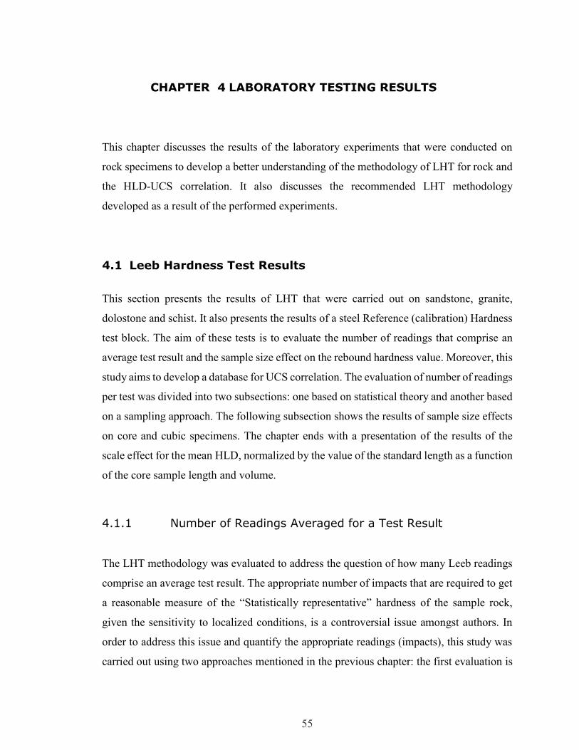
55
CHAPTER 4 LABORATORY TESTING RESULTS
This chapter discusses the results of the laboratory experiments that were conducted on
rock specimens to develop a better understanding of the methodology of LHT for rock and
the HLD-UCS correlation. It also discusses the recommended LHT methodology
developed as a result of the performed experiments.
4.1 Leeb Hardness Test Results
This section presents the results of LHT that were carried out on sandstone, granite,
dolostone and schist. It also presents the results of a steel Reference (calibration) Hardness
test block. The aim of these tests is to evaluate the number of readings that comprise an
average test result and the sample size effect on the rebound hardness value. Moreover, this
study aims to develop a database for UCS correlation. The evaluation of number of readings
per test was divided into two subsections: one based on statistical theory and another based
on a sampling approach. The following subsection shows the results of sample size effects
on core and cubic specimens. The chapter ends with a presentation of the results of the
scale effect for the mean HLD, normalized by the value of the standard length as a function
of the core sample length and volume.
4.1.1 Number of Readings Averaged for a Test Result
The LHT methodology was evaluated to address the question of how many Leeb readings
comprise an average test result. The appropriate number of impacts that are required to get
a reasonable measure of the “Statistically representative” hardness of the sample rock,
given the sensitivity to localized conditions, is a controversial issue amongst authors. In
order to address this issue and quantify the appropriate readings (impacts), this study was
carried out using two approaches mentioned in the previous chapter: the first evaluation is

56
based on statistical theory, and the second approach is based on semi-empiricist theory
“sampling”. It is relying on the Central Limit Theorem and the Law of Large Numbers.
4.1.1.1 Results of Evaluation Based on Statistical Theory
The first approach in this study, the evaluation of the Number of Readings, was based on
statistical theory. The statistical measures of 100 readings on all tested specimens
(sandstone, granite, dolostone, H-schist, V-schist and reference hardness block), including
the μ and are presented in Tables 4.1.
The results using the tested specimens (sandstone, granite, dolostone, H-schist, V-schist
and reference hardness block), for which we have 100 repeated measurements are shown
in Table 4.2. This table illustrate that, by increasing the number of impact readings the
associated margin of error decreases. In general, the LHT requires sampling effort to obtain
a relatively good estimate of the true hardness of rocks.
Table 4.1 Statistical analysis of 100 impacts on tested rocks using LHT
Statistical measure Test
block
V-
Schist
H-
Schist
Dolostone Granite Sandstone
Standard deviation 2 56.5 92.5 18 43 21
Confidence Interval at
95% ±0.11 ±9 ±15 ±9 ±8 ±4
Upper confidence limit 773 867 844 647 879 557
Lower confidence limit 764 584 447 564 863 548
Mean 770 759 710 594 879 552
Median 770 762 743 592 880 552

57
Table 4.2 Statistical details of the number of impacts that constitute a “valid” test on
tested rocks (see 3. 2.1.1).
Tested rock
Number of impacts in subset
10 20 30
Margin of error (± 𝑴𝑬)
Sandstone 13 9 8
Granite 27 19 15
Dolostone 11 8 6
H-Schist 57 40 32
V-Schist 35 25 20
Test block 1.24 0.88 0.72
4.1.1.2 Sample Size Evaluation Based on Sampling
The second approach that was used to evaluate the sample size effect is based on sampling,
relying on the Central Limit Theorem and the Law of Large Numbers. The key idea in the
Central Limit Theorem is that when a population is repeatedly sampled, the calculated
average value of the feature obtained by those specimens is equal to the true μ value, and
the Law of Large Numbers states that as a sample size grows, its mean will converge in
probability towards the average of the whole population. Moreover, because of the high
variability of the �̅� at low sample numbers, multiple “realizations” (a total of ten) of this
randomized subset study were carried out.
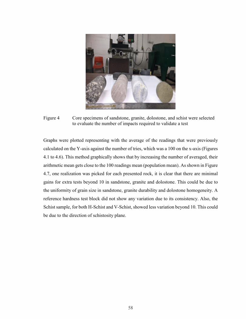
58
Figure 4 Core specimens of sandstone, granite, dolostone, and schist were selected
to evaluate the number of impacts required to validate a test
Graphs were plotted representing with the average of the readings that were previously
calculated on the Y-axis against the number of tries, which was a 100 on the x-axis (Figures
4.1 to 4.6). This method graphically shows that by increasing the number of averaged, their
arithmetic mean gets close to the 100 readings mean (population mean). As shown in Figure
4.7, one realization was picked for each presented rock, it is clear that there are minimal
gains for extra tests beyond 10 in sandstone, granite and dolostone. This could be due to
the uniformity of grain size in sandstone, granite durability and dolostone homogeneity. A
reference hardness test block did not show any variation due to its consistency. Also, the
Schist sample, for both H-Schist and V-Schist, showed less variation beyond 10. This could
be due to the direction of schistosity plane.
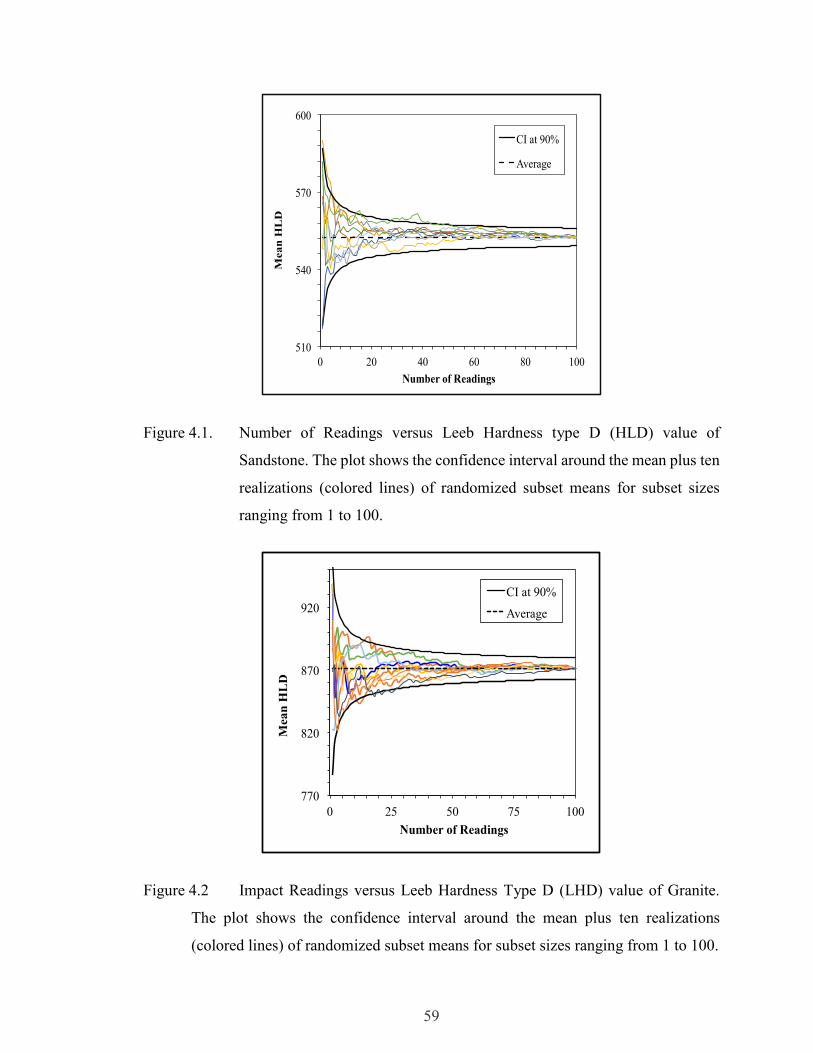
59
Figure 4.1. Number of Readings versus Leeb Hardness type D (HLD) value of
Sandstone. The plot shows the confidence interval around the mean plus ten
realizations (colored lines) of randomized subset means for subset sizes
ranging from 1 to 100.
Figure 4.2 Impact Readings versus Leeb Hardness Type D (LHD) value of Granite.
The plot shows the confidence interval around the mean plus ten realizations
(colored lines) of randomized subset means for subset sizes ranging from 1 to 100.
510
540
570
600
0 20 40 60 80 100
Mean
HL
D
Number of Readings
CI at 90%
Average
770
820
870
920
0 25 50 75 100
Mea
n H
LD
Number of Readings
CI at 90%
Average
60
Figure 4.3 Impact Readings versus Leeb Hardness Type D (HLD) value of Dolostone.
The plot shows the confidence interval around the mean plus ten realizations
(colored lines) of randomized subset means for subset sizes ranging from 1 to 100.
Figure 4.4 Number of Readings versus Leeb Hardness Type D (HLD) value of
Reference Hardness test block.
560
580
600
620
0 20 40 60 80 100
Mean
HL
D
Number of Readings
CI at 90%
Average
765
770
775
0 20 40 60 80 100
Mean
HL
D
Number of Readings
____CI at 90% ------Average

61
Figure 4.5 Number of Readings versus Leeb Hardness Type D (HLD) value of H-
Schist. The plot shows the confidence interval around the mean plus ten
realizations (colored lines) of randomized subset means for subset sizes
ranging from 1 to 100.
Figure 4.6 Number of Readings versus Leeb Hardness Type D (HLD) value of V-Schist. The
plot shows the confidence interval around the mean plus ten realizations (colored
lines) of randomized subset means for subset sizes ranging from 1 to 100.
550
650
750
850
950
0 20 40 60 80 100
Mean
HL
D
Number of Readings
_____CI at 90%
-------- Average
650
750
850
0 20 40 60 80 100
Mean
HL
D
Number of Readings
___CI at 90% -----Average
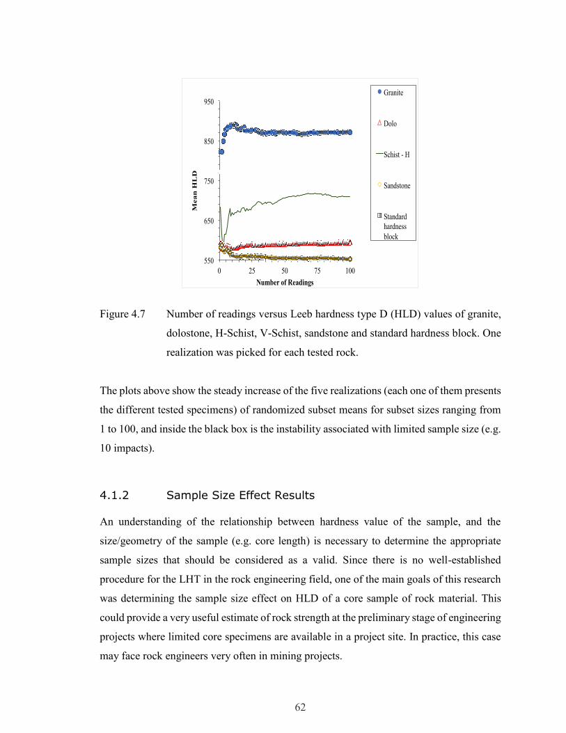
62
Figure 4.7 Number of readings versus Leeb hardness type D (HLD) values of granite,
dolostone, H-Schist, V-Schist, sandstone and standard hardness block. One
realization was picked for each tested rock.
The plots above show the steady increase of the five realizations (each one of them presents
the different tested specimens) of randomized subset means for subset sizes ranging from
1 to 100, and inside the black box is the instability associated with limited sample size (e.g.
10 impacts).
4.1.2 Sample Size Effect Results
An understanding of the relationship between hardness value of the sample, and the
size/geometry of the sample (e.g. core length) is necessary to determine the appropriate
sample sizes that should be considered as a valid. Since there is no well-established
procedure for the LHT in the rock engineering field, one of the main goals of this research
was determining the sample size effect on HLD of a core sample of rock material. This
could provide a very useful estimate of rock strength at the preliminary stage of engineering
projects where limited core specimens are available in a project site. In practice, this case
may face rock engineers very often in mining projects.
550
650
750
850
950
0 25 50 75 100
Mean
HL
D
Number of Readings
Granite
Dolo
Schist - H
Sandstone
Standard
hardness
block
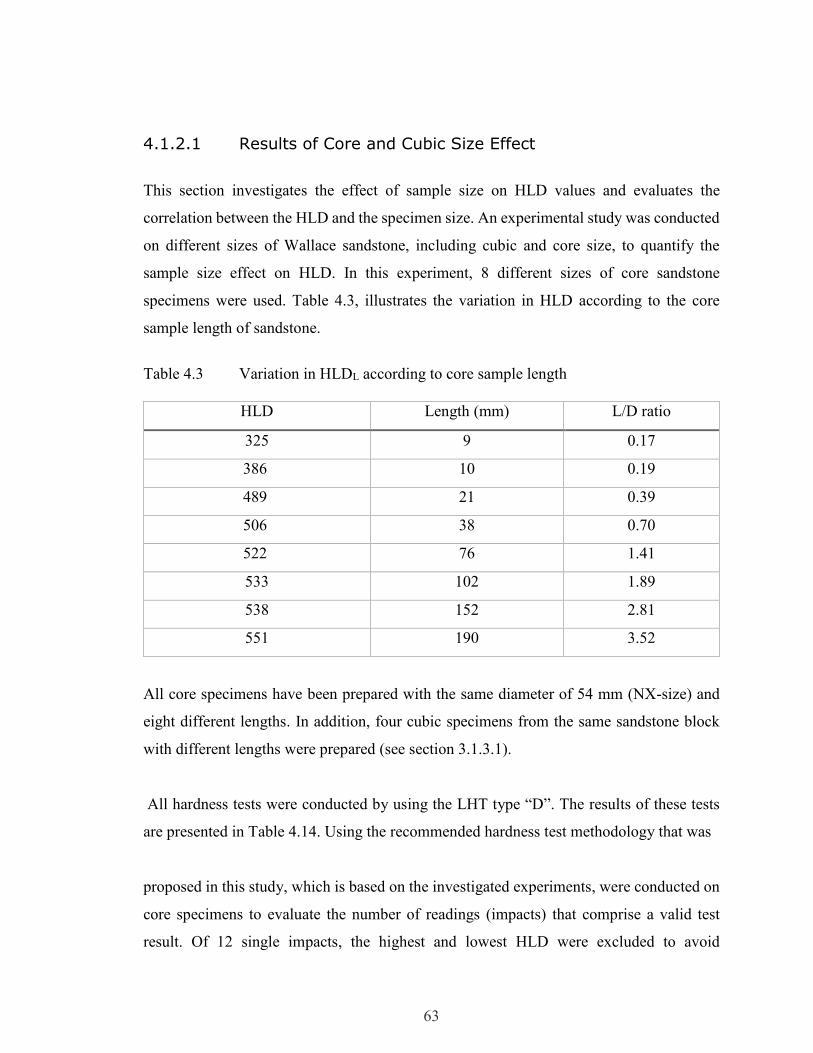
63
4.1.2.1 Results of Core and Cubic Size Effect
This section investigates the effect of sample size on HLD values and evaluates the
correlation between the HLD and the specimen size. An experimental study was conducted
on different sizes of Wallace sandstone, including cubic and core size, to quantify the
sample size effect on HLD. In this experiment, 8 different sizes of core sandstone
specimens were used. Table 4.3, illustrates the variation in HLD according to the core
sample length of sandstone.
Table 4.3 Variation in HLDL according to core sample length
HLD Length (mm) L/D ratio
325 9 0.17
386 10 0.19
489 21 0.39
506 38 0.70
522 76 1.41
533 102 1.89
538 152 2.81
551 190 3.52
All core specimens have been prepared with the same diameter of 54 mm (NX-size) and
eight different lengths. In addition, four cubic specimens from the same sandstone block
with different lengths were prepared (see section 3.1.3.1).
All hardness tests were conducted by using the LHT type “D”. The results of these tests
are presented in Table 4.14. Using the recommended hardness test methodology that was
proposed in this study, which is based on the investigated experiments, were conducted on
core specimens to evaluate the number of readings (impacts) that comprise a valid test
result. Of 12 single impacts, the highest and lowest HLD were excluded to avoid
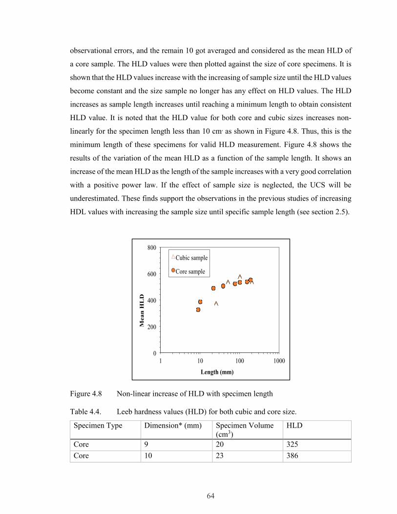
64
observational errors, and the remain 10 got averaged and considered as the mean HLD of
a core sample. The HLD values were then plotted against the size of core specimens. It is
shown that the HLD values increase with the increasing of sample size until the HLD values
become constant and the size sample no longer has any effect on HLD values. The HLD
increases as sample length increases until reaching a minimum length to obtain consistent
HLD value. It is noted that the HLD value for both core and cubic sizes increases non-
linearly for the specimen length less than 10 cm, as shown in Figure 4.8. Thus, this is the
minimum length of these specimens for valid HLD measurement. Figure 4.8 shows the
results of the variation of the mean HLD as a function of the sample length. It shows an
increase of the mean HLD as the length of the sample increases with a very good correlation
with a positive power law. If the effect of sample size is neglected, the UCS will be
underestimated. These finds support the observations in the previous studies of increasing
HDL values with increasing the sample size until specific sample length (see section 2.5).
Figure 4.8 Non-linear increase of HLD with specimen length
Table 4.4. Leeb hardness values (HLD) for both cubic and core size.
Specimen Type
Dimension* (mm) Specimen Volume
(cm3)
HLD
Core 9 20 325
Core 10 23 386
0
200
400
600
800
1 10 100 1000
Mea
n H
LD
Length (mm)
Cubic sample
Core sample

65
Specimen Type
Dimension* (mm) Specimen Volume
(cm3)
HLD
Core 22 49 488
Core 38 87 506
Core 76 174.5 522
Core 102 233 533
Core 152 349 538
Core 190.5 436 551
Cube 25 16 373
Cube 51 131 534
Cube 102 1049 576
Cube 203 8390 535
*Length of 54 mm diameter core or cube side length
4.1.2.2 Results of Scale Effect for the Mean Normalized HLD
This subsection presents the results of the scale effect for the mean HLD normalized by the
value of the standard length of 102 mm (101.6 mm, precisely) as a function of sample
length that showed no effect of nonlinearly increasing on its hardness value. Here again, an
increase in the value of the HLD as the length increases is observed. Figure 4.9 illustrates
the influence of core sample length (HLDL) related to standardized value (HLD102mm). For
specimen size correction of specimens less than L/D=1.5, the following formula is
proposed:
𝐻𝐿𝐷𝐿 = 0.98 𝐿/𝐷0.2 × 𝐻𝐿𝐷102𝑚𝑚 ..
[5.1]
Table 4.13 shows the variation in HLD values according to the core sample length of
sandstone and the L/D ratio.

66
Figure 4.9 Influence of core sample size HLDL related to HLD102mm
In short, there is an observed nonlinear relationship between sample size and HLD below
1.5 L/D ratio and it was found to be constant above 1.5 L/D ratio. Small sample size could
be corrected for, using the nonlinear relationship.
4.2 UCS TESTING RESULTS
This section contains the results of the UCS tests that were carried out on core specimens
of different rock types, to corresponding HLD values, in which they used to evaluate the
UCS and HLD correlation. The specimens include the following rocks: granite, dolomite,
coal-sandstone, greywacke, limestone, and sandstone. The number of specimens that have
been tested are as following: 10 schist, 3 granite, 3 dolostone, 4 coal sandstone, 3
greywacke, 3 limestone, 2 sandstones, 10 schist with horizontal foliation to load direction,
and 6 Schist 2 Mafic dyke with vertical foliation to load direction. The total of 46 rock core
specimens was tested at Dalhousie University. The UCS tests began in March 2015 and
lasted until October 2015.
0
0.5
1
1.5
0 1 2 3 4
HL
DL /
HL
D 1
02
mm
L / D ratio

67
4.2.1 Schist Results
The UCS tests were performed on ten Schist specimens (Figure 4.10), after preparing the
specimens according to the ASTM preparation procedure. The UCS test results ranged from
17 to 69 MPa. Young's Modulus (GPa) ranged from 4 to 11. The Poisson's ratio (ν), ranged
from 0.2 to 0.3, as seen in Table 4.5. In Table 4.5, the mechanical properties of schist
specimens are presented. In table 4.6, the geometric properties of schist sample are
presented. The lithology description of the selected tested is given in Table 4.7. Table 4.7.1
shows the mechanical properties results of stress-strain curves of schist. Figure 4.11 shows
some of the Stress–Strain curves of these core specimens. The rest of the stress-strain
curves for schist rock were put in the Appendix B.
68
Table 4.5 Mechanical properties for schist specimens.
(a) (b)
(c)
(d) (e)
Figure 4.10 (a, b, c, d, e) Schist core specimens; the strain gauge pairs were installed at the
opposite sides to measure the deformation caused by the UCS tests.

69
Hole # UCS
(MPa)
Force
(kN)
Young's
modulus
(GPa)
Failure mode Poisson's
ratio, ν
RMUG14-252, Box-8, #1 43 44237 10 Structure 0.26
RMUG14-252, Box-8. #2 27 27374 5.5 Structure 0.24
RMUG14-252, Box-15, #1 17 17237 4.5 Structure 0.22
RMUG14-249, Box-3, #1 61 62806 5 Split 0.21
RMUG14-249, Box-14#2 38 39441 6.5 Split 0.22
RMUG14-249, Box-22, #5 69 70713 11 Split 0.20
RMUG14-249, Box-22, #6 27 28124 4 Structure 0.3
RMUG14-249, Box-23, #7 50 50927 7 Structure 0.21
Table 4.6 Geometric properties of schist specimens
Hole # Length
(Mm)
Dia
(Mm) L/D
Area
(Mm2)
Weight
(g)
Volume
(Cm3)
RMUG14-252, Box-8, 1 81 36 2 1027 243 83
RMUG14-252, Box-8, 2 80 36 2 1024 230 82
RMUG14-252, Box-15, 1 80 36 2 1026 233 82
RMUG14-249, Box-3, 1 80 36 2 1028 232 82
RMUG14-249, Box-14, 2 80 36 2 1029 229 83
RMUG14-249, Box-22, 5 80 36 2 1028 252 82
RMUG14-249, Box-22, 6 80 36 2 1027 248 83
RMUG14-249, Box-23, 7 80 36 2 1026 271 82
Table 4.7 Lithology for schist specimens.

70
Hole # Lithology Test type Rock type Foliation
core Axis
RMUG14-252,
Box-8. #2
Tzu- Sericite
Schist
UCS Schist 45
RMUG14-252,
Box-15, #1
Tzu- Sericite
Schist
UCS Schist 45
RMUG14-249,
Box-3, #1
Qtz- Sericite
Schist
UCS Schist 40
RMUG14-249,
Box-22, #5
Qtz- Chlorite
Schist
UCS Weak-Moderate-
Ore ZONE
45
RMUG14-249,
Box-22, #6
Qtz- Chlorite
Schist
UCS Weak-Moderate-
Ore ZONE
45
RMUG14-249,
Box-23, #7
Qtz- Chlorite
Schist
UCS Weak-Moderate-
Ore ZONE
35
RMUG14-252,
Box-8, #1
Qtz- Chlorite
Schist
UCS Weak-Moderate-
Ore ZONE
35
Table 4.7.1 Mechanical properties results of stress-strain curves of schist
Hole # Sample
number
Strain
%
Area
(mm2)
MR=
E/UCS
Weight
(g)
Axial
strain
%*10 at
50%
Lateral
strain
%*10 at
50%
RMUG14-
252,Box-8
1 0.3 1027.37 232.24 243.33 0.4665 0.12
RMUG14-
252,Box-8
2 0.2 1023.59 205.65 230.82 0.529 0.01
RMUG14-
252,Box-15
1 0.2 1025.48 267.70 233.19 0.2555 0.02
RMUG14-
249,Box-3
1 0.8 1027.56 81.80 232.16 0.506 0.10
RMUG14-
249,Box-14
2 0.4 1028.88 169.56 229.18 0.651 0.06
RMUG14-
249,Box-19
3 0.3 1027.75 207.18 224.11 0.2595 0.05
RMUG14-
249,Box-19
4 0.1 1027.94 471.69 227.98 0.248 0.05
RMUG14-
249,Box-22
5 0.2 1027.94 159.90 251.56 0.763 0.15
RMUG14-
249,Box-22
6 0.4 1026.80 141.47 240.73 0.471 0.23
RMUG14-
249,Box-23
7 0.3 1025.86 134.29 271.01 0.372 0.05

71
(a) RMUG 14-249, Box-22, sample 6 (b) RMUG14-249, Box-22, sample 5
Figure 4.11(a and b) Stress-Strain curves of schist specimens, using strain gauge and
Linear Variable Differential Transformer (LVDT), which are transducers to measure the
displacement for schist core specimens under UCS tests. LVDT is able to produce for
small displacement.
*Note: The rest of the stress-strain curves for schist rock were put in the appendix.
0
5
10
15
20
25
30
-1 0 1
UC
S (
MP
a)
% Strain
Axial strain
Lateral strain
LVDT
0
10
20
30
-1 0 1
UC
S (
MP
a)
% Strain
Lateral strain
LVDT
Axial strain

72
Figure 4.12 Schist specimens with vertical schistosity (sv1, sv2, sv3, sv4, sv5)
Figure 4.13 Schist specimens with horizontal schistosity (sh4, sh5, sh6, sh7, sh8, sh9,
sh10, sh11, sh12 and sh13)
Figure 4.14 Tested Schist specimens

73
4.2.2 Other Rocks
The UCS tests were carried out on a number of core specimens. The condition of these
specimens before UCS testing is presented in a table with some comments (attached to
Appendix 2). The description of Schist specimens after preparation is showed in a table
(attached to Appendix 2). As a result of these tests, the UCS was ranged from 27 to 220
MPa. Some specimens showed shear failure mode, others showed an axial splitting. The
Young’s Modules were ranged from 5 to 21 MPa, (see Appendix 2). The geometric details
of tested specimens are given in a table (attached to Appendix 2).
4.3 Chapter Summary
This chapter presented the results of laboratory experiments that were conducted on
different rock types to develop methodology and correlation for UCS. The results of the
laboratory experiments include the UCS tests and the LHT. These two tests help to develop
a Leeb test methodology by evaluating the number of impacts that give a valid test, and
examine the sample size effect on HLD for both core and cubic specimens of rock material.
In addition, these tests help to develop correlation for UCS. The following correlations
were presented: the correlation between the HLD and the specimen size, the correlation
between the HLD and the specimen length, and the correlation between the HLD and the
L/D ratio. Moreover, the plots of impact readings versus LHD values for tested specimens
were presented with confidence intervals. This could provide a useful estimate of rock
strength for engineering projects.
74
CHAPTER 5 ANALYSIS
Some scholars of rock engineering agree on the potential in studying and understanding the
relationship between the UCS results and the Leeb hardness for intact rocks. Recently,
many research studies, have demonstrated that the impact-rebound method has some
correlation to UCS. However, there has been no universal correlation established for all
rock types.
In order to increase confidence in an estimation parameter, it is important to analyze the
same measurements that were conducted many times in different experiments. The greater
the statistical strength (i.e. more measurements) the better the UCS estimate will be. Taking
multiple measurements also allows one to better estimate the uncertainty in UCS
measurements by checking how reproducible the measurements are. How precise UCS
estimates of rock material are depends on the spread of the measurements (standard
deviation) and the number (N) of repeated measurements that were taken. Therefore,
statistical analysis is required to have a more sophisticated estimate of the uncertainty in
the UCS measurement.
The main purpose of this study is to develop an understanding regarding the relationship
between HLD and UCS. In order to develop such a relationship, one that can be used in the
field, the evaluation of UCS-HLD correlation needed to be performed, and the results
needed to be analyzed on a statistical basis. This provides a convenient means to obtain
improved accuracy in field estimation of UCS. For that reason, this chapter contains a
discussion of analysis. Included in this chapter are required statistical measurements on the
database, which were collected from a thorough literature review and the results of
laboratory tests. This is done in order to determine how well the regression line fits the;
such values as (R2) and the S are considered, and then the correlation of UCS-HLD is
plotted to establish an equation relating the relationship between UCS and

75
HLD. In addition, the three main rock types are analyzed in subsections and the plot of
UCS-HLD correlations are presented. This chapter ends with Leeb hardness analysis and
comparison between HLD and Schmidt Hammer. The final section in this chapter reviews
a conference paper studying sandstone (attached to the Appendix A). Statistical analysis
(Regression, T-Test, F-Test and residual) has been used to develop the relationship between
the mean value of hardness tests and their corresponding rock strengths to improve the LHT
procedure. Then, the plots of UCS-HLD correlations were presented.
5.1 UCS–HLD CORRELATION
In order to quantitatively analyze and develop the relationship between HLD values and
UCS, regression analyses were used. There are different curves, such as linear, logarithmic,
power and polynomial, which can be used to study the correlation between the independent
and dependent variables. The coefficient of determination (R2), which is produced by the
best-fit curve, is the measure of the variability proportion of one variable to the other
variable (Sheskin, 2000). Once the regression best-fit curve and the value of R2 have been
determined, an examiner will then pick which best curve fits in the appropriate way.
Usually, the most appropriate curve is the one with the relatively highest R2 value. Based
on the literature review, the exponential curve is expected between UCS, and HLD.
5.1.1 Database
A database was developed from the literature review (Table 5.1), BGC Engineering project
files (provided by D Kinakin, pers. comm.) and the results of laboratory tests carried out as
part of this study. The developed database and the results of laboratory tests were then
verified. They cover a wide range of the UCS values of rock material from around the
world. This will help to establish how accurately the UCS of rock material could be
obtained by using a portable LHT.

76
Two statistical analysis models were performed in order to find the best correlation with
the lowest S, which is a useful measure to assess the accuracy of the predictions. The first
analysis is modeled by a power function; the second one is modeled by an exponential
function. The curve was selected based on previous knowledge from the literature about
the response curve's shape between UCS and HLD. The power model in Table 5.3 showed
a slightly lower S with an R² of 0.70. These analyses were performed using the Minitab
software (Ryan et al., 2004).
Figure 5.1 shows the relationship between HLD, and UCS for specimens tested both in the
present study and collected from the literature. Such a large scatter of as seen in Figure 5.1
could be attributed to variation in Young's Modulus in specimens that have the same UCS
value and rock conditions. In spite of the scatter in, there is a tendency for HLD to increase
with increasing UCS. The points cover a wide range of UCS values, ranged from 3 MPa
(green schist, Kawasaki et al., 2002) to 285 MPa that were observed in metavolcanic rocks.
These values represent the wide practical range found in the field.
The HLD and UCS proposed correlation of previous studies were presented in Figure 5.2.
The comparison between UCS-HLD improved database correlation and the correlation
proposed by Verwaal & Mulder (1993) are presented in Figure 5.3. The proposed
correlation in this study showed R2 of 0.70 based on 311 UCS tests, while a proposed
correlation suggested by Verwaal & Mulder (1993) showed R2 of 0.77 based on only 27
UCS tests.

77
Figure 5.1 UCS-HLD correlation of the developed database.
Table 5.1 Description of rock specimens and number of tests from previous studies using
the Leeb hardness test (LHT) that were used to develop the database
Database
UCS = 1.57E-05 HLD2.419
R² = 0.70
S=40
0
50
100
150
200
250
300
0 200 400 600 800 1000
UC
S (
MP
a)
HLD
Source Number of
tests
Rock type
Verwaal and Mulder, 1993 27 Sandstone, limestone gypsum, dolostone,
marble, granite, calcarenite
Hack et al 1993 15 Sandstone, granite, Limestone
Asef, M, 1995 63 gypsum, gypsum and silty clay,
conglomerated, sandstone, dolomitic
calcilutite, limestone muds-calcilutite,
sandy clay, dolomitic breccia, limestone
calcarenite layers, granodiorite, thinly
bedded dolomite, calcilutite
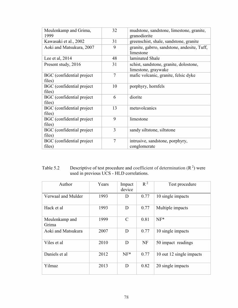
78
Table 5.2 Descriptive of test procedure and coefficient of determination (R 2) were
used in previous UCS - HLD correlations.
Author Years Impact
device
R 2 Test procedure
Verwaal and Mulder 1993 D 0.77 10 single impacts
Hack et al 1993 D 0.77 Multiple impacts
Meulenkamp and
Grima
1999 C 0.81 NF*
Aoki and Matsukura 2007 D 0.77 10 single impacts
Viles et al 2010 D NF 50 impact readings
Daniels et al 2012 NF* 0.77 10 out 12 single impacts
Yilmaz 2013 D 0.82 20 single impacts
Meulenkamp and Grima,
1999
32 mudstone, sandstone, limestone, granite,
granodiorite
Kawasaki et al., 2002 31 greenschist, shale, sandstone, granite
Aoki and Matsukura, 2007 9 granite, gabrro, sandstone, andesite, Tuff,
limestone
Lee et al, 2014 48 laminated Shale
Present study, 2016 31 schist, sandstone, granite, dolostone,
limestone, graywake
BGC (confidential project
files)
7 mafic volcanic, granite, felsic dyke
BGC (confidential project
files)
10 porphyry, hornfels
BGC (confidential project
files)
6 diorite
BGC (confidential project
files)
13 metavolcanics
BGC (confidential project
files)
9 limestone
BGC (confidential project
files)
3 sandy siltstone, siltstone
BGC (confidential project
files)
7 intrusive, sandstone, porphyry,
conglomerate
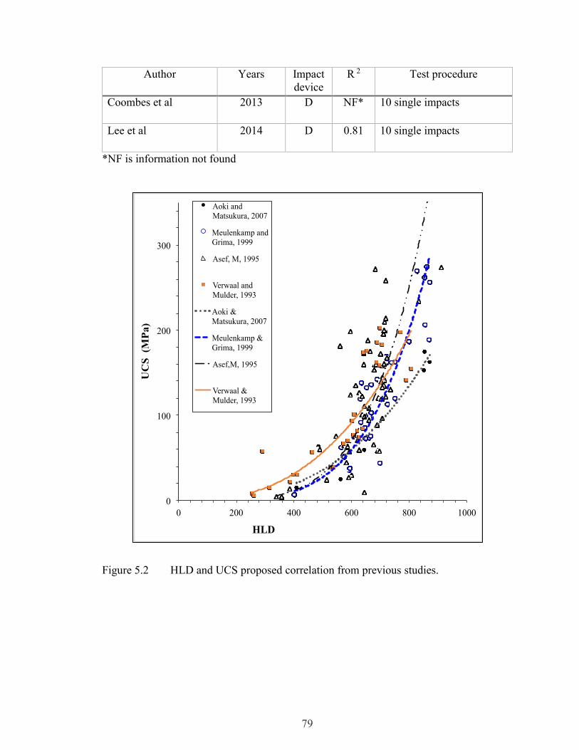
79
Author Years Impact
device
R 2 Test procedure
Coombes et al 2013 D NF* 10 single impacts
Lee et al 2014 D 0.81 10 single impacts
*NF is information not found
Figure 5.2 HLD and UCS proposed correlation from previous studies.
0
100
200
300
0 200 400 600 800 1000
UC
S (M
Pa
)
HLD
Aoki and
Matsukura, 2007
Meulenkamp and
Grima, 1999
Asef, M, 1995
Verwaal and
Mulder, 1993
Aoki &
Matsukura, 2007
Meulenkamp &
Grima, 1999
Asef,M, 1995
Verwaal &
Mulder, 1993

80
To test the models, an analysis of variance was conducted. Parameters for the analysis of
variance for two models are given in Table 5.3. Since the power model had lower S, it is
concluded that this model better represents the than exponential model.
In this study, an exponential model of the set was selected. Using information from the
literature about the shape of the response curve and the behavior of the physical
properties, an exponential growth curve was selected with the following expected
function form for one parameter (UCS) and one predictor (HLD):
𝐔𝐂𝐒 = 𝛉𝟏 × 𝒆 (𝛉𝟐 × 𝐇𝐋𝐃) [5-1]
Where the θ1 and θ 2 represent fit parameters and HLD represents the predictor. The trend
expressed by the nonlinear model is described as:
𝐔𝐂𝐒 (𝐌𝐏𝐚) = 𝟑. 𝟏𝟑𝟑𝟓 𝐄𝐗𝐏𝟎.𝟎𝟎𝟓𝟏 𝐇𝐋𝐃 [5-2]
The R2 coefficient of 0.67 reflects the degree of scatter in the database. This shows UCS
can be predicted with a reasonable degree of accuracy using the HLD. S was used to assess
how well the regression model predicts the response between two models (Table 5.3). The
lower the value of S, the better the model predicts the response (UCS). In order to compare
the two prediction models, the following statistical performance indexes were used: The S,
SSE, and MSE (see 3.2.2.1).
Comparing the exponential model to the power model, it is observed that the power model
equation has the lowest S value which indicates the best fit. For the power model, S is
calculated as 40, which indicates that the actual points are within a standard difference of
40 MPa (UCS) from the regression line which represents the predicted value (Table 5.3).
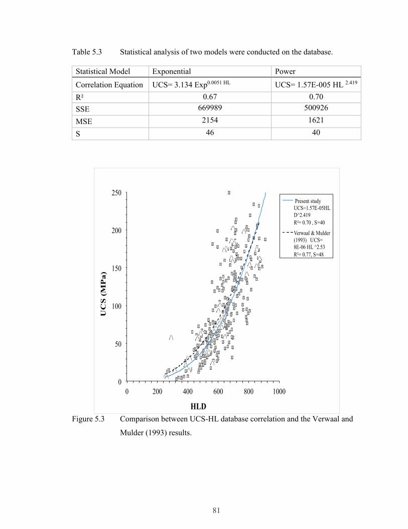
81
Table 5.3 Statistical analysis of two models were conducted on the database.
Statistical Model Exponential Power
Correlation Equation UCS= 3.134 Exp0.0051 HL UCS= 1.57E-005 HL 2.419
R² 0.67 0.70
SSE 669989 500926
MSE 2154 1621
S 46 40
Figure 5.3 Comparison between UCS-HL database correlation and the Verwaal and
Mulder (1993) results.
0
50
100
150
200
250
0 200 400 600 800 1000
UC
S (
MP
a)
HLD
Present study
UCS=1.57E-05HL
D^2.419
R²= 0.70 , S=40
Verwaal & Mulder
(1993) UCS=
8E-06 HL ^2.53
R²= 0.77, S=48
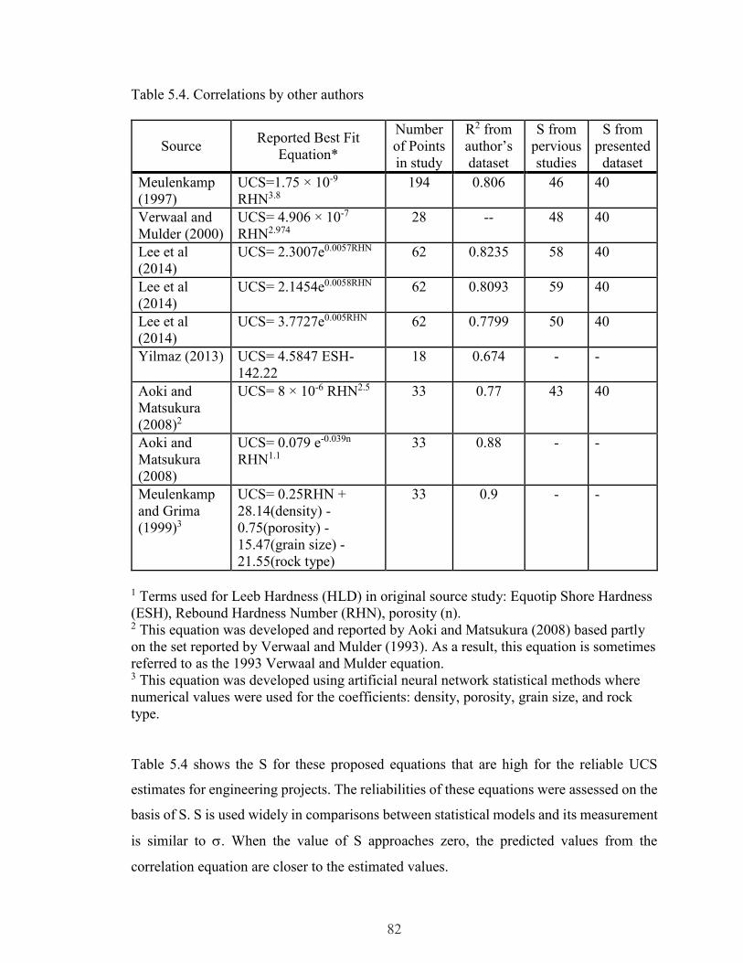
82
Table 5.4. Correlations by other authors
Source Reported Best Fit
Equation*
Number
of Points
in study
R2 from
author’s
dataset
S from
pervious
studies
S from
presented
dataset
Meulenkamp
(1997)
UCS=1.75 × 10⁻⁹
RHN3.8
194 0.806 46 40
Verwaal and
Mulder (2000)
UCS= 4.906 × 10⁻⁷
RHN2.974
28 -- 48 40
Lee et al
(2014)
UCS= 2.3007e0.0057RHN 62 0.8235 58 40
Lee et al
(2014)
UCS= 2.1454e0.0058RHN 62 0.8093 59 40
Lee et al
(2014)
UCS= 3.7727e0.005RHN 62 0.7799 50 40
Yilmaz (2013) UCS= 4.5847 ESH-
142.22
18 0.674 - -
Aoki and
Matsukura
(2008)2
UCS= 8 × 10⁻⁶ RHN2.5 33 0.77 43 40
Aoki and
Matsukura
(2008)
UCS= 0.079 e-0.039n
RHN1.1
33 0.88 - -
Meulenkamp
and Grima
(1999)3
UCS= 0.25RHN +
28.14(density) -
0.75(porosity) -
15.47(grain size) -
21.55(rock type)
33 0.9 - -
1 Terms used for Leeb Hardness (HLD) in original source study: Equotip Shore Hardness
(ESH), Rebound Hardness Number (RHN), porosity (n). 2 This equation was developed and reported by Aoki and Matsukura (2008) based partly
on the set reported by Verwaal and Mulder (1993). As a result, this equation is sometimes
referred to as the 1993 Verwaal and Mulder equation. 3 This equation was developed using artificial neural network statistical methods where
numerical values were used for the coefficients: density, porosity, grain size, and rock
type.
Table 5.4 shows the S for these proposed equations that are high for the reliable UCS
estimates for engineering projects. The reliabilities of these equations were assessed on the
basis of S. S is used widely in comparisons between statistical models and its measurement
is similar to . When the value of S approaches zero, the predicted values from the
correlation equation are closer to the estimated values.
83
5.1.2 Three Rock Types
This section further develops a LHT procedure that can be used for field evaluation of UCS,
to correlate UCS with HLD, which is the main point of this study, thereby providing a
convenient means to obtain improved accuracy in the field estimation of UCS. This section
contains a discussion of the analysis that was conducted on the three main rock types
(igneous, metamorphic and sedimentary), collected from literature review and the results
of laboratory tests which cover a wide range of the UCS values of rock material around the
world, to establish how accurately the UCS of three rock types could be obtained by using
a portable HLT.
Figure 5.4 demonstrates a comparison of HLD measured between three rock types. Even
though these rock specimens are from the same designation of rocks (igneous), there is
considerable scatter between the UCS values for each specimen. This could be attributed
to variation in cementing material and mineral hardness. The shapes of the UCS-HLD
curves are similar in each rock types, as shown in Figure 5.5.
Igneous specimens have HLD ranging from 409 to 911 HL with a UCS of 16 (Tuff, a
porous rock, Aoki and Matsukura, 2007) to 275 MPa, (granodiorite, Meulenkamp and
Grima, 1999). Sedimentary rocks have HLD that range from 255 to 833 HL, with UCS
values of 4 (gypsum and salty clay) to 220 MPa, (greywacke). Metamorphic specimens
have HLD ranging from 265 to 912 HL with UCS values of 3 for greenschist, as determined
in Kawasaki et al (2002), and 285 MPa, (metavolcanics).
Figure 5.5 presents the correlation equations of all three rock types, with R2 values. In
general, there is an increase in UCS with increasing HLD, despite the fact that the
specimens used to develop the relationship are differentiated by formation sites and
weathering. The best-fit regression lines were plotted for the UCS-HLD correlation of all
rock types, and are presented in figure 5.6. The R2 value for the sedimentary rock is 0.71,
and 0.83 for the metamorphic rocks. For igneous rocks, however, the R2 value (0.56) is not

84
high. As seen in Figure 5.7, there are scattered around the best-fit curve; therefore, it could
be said that the R2 value is unreliable (see Table 5.5).
It was observed that there was one anomalous UCS value, (285 MPa), which is the sample
of metavolcanics. In general, igneous rocks have a high UCS value relative to other rock
types.
Figure 5.4 Comparison of three rock types (igneous, metamorphic, sedimentary)
0
50
100
150
200
250
300
0 200 400 600 800 1000
UC
S (
MP
a)
HLD
Igneous
Sedimentary
Metamorphic
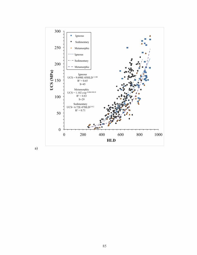
85
a)
Igneous
UCS = 9.698E-05HLD 2.140
R² = 0.65
S=45
Sedimentary
UCS= 6.72E-07HLD2.912
R² = 0.71
Metamorphic
UCS = 1.102 exp 0.0061HLD
R² = 0.83
S=29
0
50
100
150
200
250
300
0 200 400 600 800 1000
UC
S (
MP
a)
HLD
Igneous
Sedimentary
Metamorphic
Igneous
Sedimentary
Metamorphic

86
b)
Figure 5.5 (a, b) Three rock types proposed correlations compared with the
proposed database correlation.
Igneous
UCS = 9.698E-05 HLD 2.140
R² = 0.65
S=45
Database
UCS = 1.57E-05 HLD 2.419
R² = 0.702
S=40
Sedimentary
UCS = 6.72E-07 HLD 2.912
R² = 0.71
S=33
Metamorphic
UCS = 1.10 exp 0.006HLD
R² = 0.83
S=29
0
50
100
150
200
250
300
0 200 400 600 800 1000
UC
S (
MP
a)
HLD
Igneous
Database
Sedimentary
Metamorphic

87
Figure 5.6 Metamorphic rocks proposed correlation
Metamorphic
UCS = 1.102 EXP 0.0061HLD
R² = 0.83
S=29
0
50
100
150
200
250
300
0 200 400 600 800 1000
UC
S (
MP
a)
HLD
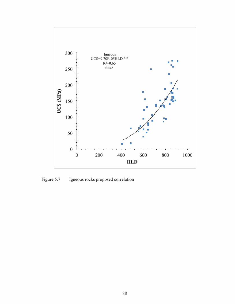
88
Figure 5.7 Igneous rocks proposed correlation
0
50
100
150
200
250
300
0 200 400 600 800 1000
UC
S (
MP
a)
HLD
Igneous
UCS=9.70E-05HLD 2.14
R2=0.65
S=45

89
Figure 5.8 Sedimentary rocks proposed correlation
Table 5.5 Proposed correlation equations with coefficient of determination (R2) in
present study.
Rock Type Recommended Equations R2
Presented database UCS= 1.57E-05 HLD 2.419 0.70
Rock Classification
Sedimentary UCS= 6.72E-07 * HLD2.91 0.71
Metamorphic UCS= 1.102 EXP 0.0061HLD 0.83
Igneous UCS= 9.70E-05 HLD 2.14 0.65
Specific Rock
Sandstone UCS= 9E-07 HLD 2.839 0.75
Limestone UCS= 8E-07 HLD 2.896 0.50
Schist UCS= 6E-06 HLD 2.479 0.73
0
50
100
150
200
250
0 200 400 600 800 1000
UC
S (
MP
a)
HLD
Sedimentary
UCS=6.716E-07HLD 2.912
R 2 =0.71
S=33

90
Table 5.6 Leeb Hardness (HLD) and UCS correlation parameters.
Set R2 Equation Coefficients
a b
All rock types 0.70 0.3 3
Sandstone 0.75 0.9 2.84
Sedimentary Rocks* 0.71 0.1 3.18
Metamorphic Rocks 0.79 0.3 2.98
Igneous Rocks 0.65 3 2.64
*Including sandstone
Table 5.7 presents the statistical analysis for HLD values of the 3 rock types, including
from the proposed database. It can be seen that the metamorphic rocks showed a higher
compared to the other rock types. This could be due to the existence of foliation in
metamorphic rocks. Metamorphic rock texture could be foliated or nonfoliated; nonfoliated
ones are usually uniform in texture, and contain only one mineral.
Table 5.7 Statistical analysis for LHD of three main rock types including proposed
database.
Rock type Sedimentary Metamorphic Igneous Database
Mean 610 645 745 639
Standard deviations 110.5 167 127 132
Confidence interval at95% 15 50 34 15
Number of sample 209 43 55 311
5.2 Leeb Hardness Analysis
As evidenced by this study, HLD shows a reasonable correlation with UCS. Table 5.8
provides a classification of HLD that was generated for classifying the HLD values based
on analyzing the presented study database. It provides a useful basis for classifying HLD
and
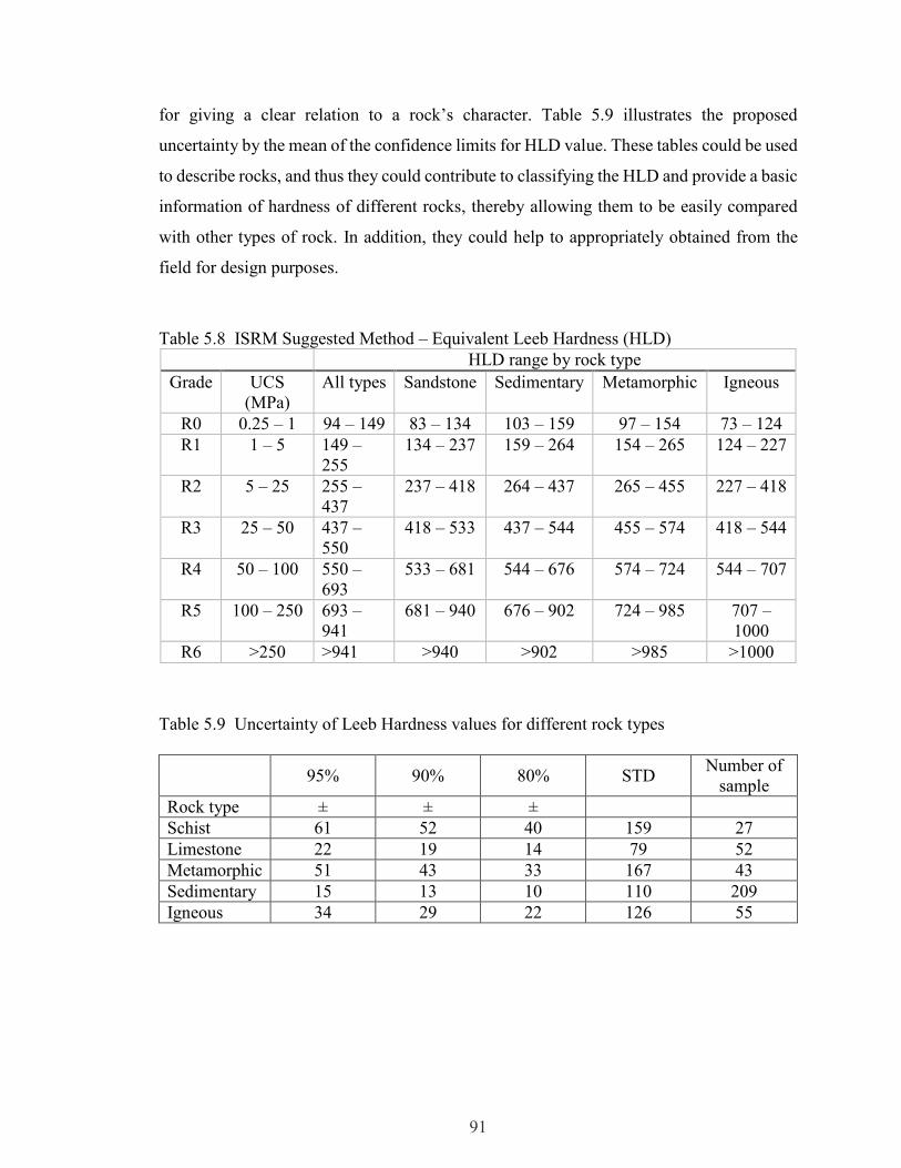
91
for giving a clear relation to a rock’s character. Table 5.9 illustrates the proposed
uncertainty by the mean of the confidence limits for HLD value. These tables could be used
to describe rocks, and thus they could contribute to classifying the HLD and provide a basic
information of hardness of different rocks, thereby allowing them to be easily compared
with other types of rock. In addition, they could help to appropriately obtained from the
field for design purposes.
Table 5.8 ISRM Suggested Method – Equivalent Leeb Hardness (HLD)
HLD range by rock type
Grade UCS
(MPa)
All types Sandstone Sedimentary Metamorphic Igneous
R0 0.25 – 1 94 – 149 83 – 134 103 – 159 97 – 154 73 – 124
R1 1 – 5 149 –
255
134 – 237 159 – 264 154 – 265 124 – 227
R2 5 – 25 255 –
437
237 – 418 264 – 437 265 – 455 227 – 418
R3 25 – 50 437 –
550
418 – 533 437 – 544 455 – 574 418 – 544
R4 50 – 100 550 –
693
533 – 681 544 – 676 574 – 724 544 – 707
R5 100 – 250 693 –
941
681 – 940 676 – 902 724 – 985 707 –
1000
R6 >250 >941 >940 >902 >985 >1000
Table 5.9 Uncertainty of Leeb Hardness values for different rock types
95% 90% 80% STD Number of
sample
Rock type ± ± ±
Schist 61 52 40 159 27
Limestone 22 19 14 79 52
Metamorphic 51 43 33 167 43
Sedimentary 15 13 10 110 209
Igneous 34 29 22 126 55
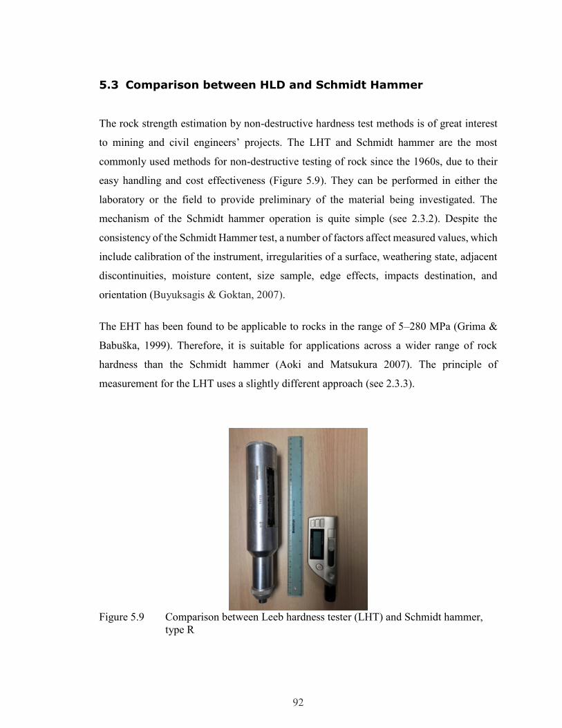
92
5.3 Comparison between HLD and Schmidt Hammer
The rock strength estimation by non-destructive hardness test methods is of great interest
to mining and civil engineers’ projects. The LHT and Schmidt hammer are the most
commonly used methods for non-destructive testing of rock since the 1960s, due to their
easy handling and cost effectiveness (Figure 5.9). They can be performed in either the
laboratory or the field to provide preliminary of the material being investigated. The
mechanism of the Schmidt hammer operation is quite simple (see 2.3.2). Despite the
consistency of the Schmidt Hammer test, a number of factors affect measured values, which
include calibration of the instrument, irregularities of a surface, weathering state, adjacent
discontinuities, moisture content, size sample, edge effects, impacts destination, and
orientation (Buyuksagis & Goktan, 2007).
The EHT has been found to be applicable to rocks in the range of 5–280 MPa (Grima &
Babuška, 1999). Therefore, it is suitable for applications across a wider range of rock
hardness than the Schmidt hammer (Aoki and Matsukura 2007). The principle of
measurement for the LHT uses a slightly different approach (see 2.3.3).
Figure 5.9 Comparison between Leeb hardness tester (LHT) and Schmidt hammer,
type R
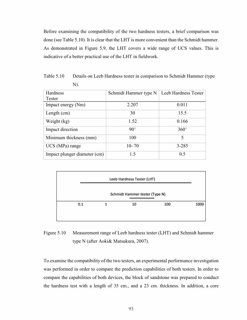
93
Before examining the compatibility of the two hardness testers, a brief comparison was
done (see Table 5.10). It is clear that the LHT is more convenient than the Schmidt hammer.
As demonstrated in Figure 5.9, the LHT covers a wide range of UCS values. This is
indicative of a better practical use of the LHT in fieldwork.
Table 5.10 Details on Leeb Hardness tester in comparison to Schmidt Hammer (type
N).
Hardness
Tester
Schmidt Hammer type N Leeb Hardness Tester
Impact energy (Nm) 2.207 0.011
Length (cm) 30 15.5
Weight (kg) 1.52 0.166
Impact direction 90° 360°
Minimum thickness (mm) 100 5
UCS (MPa) range 10- 70 3-285
Impact plunger diameter (cm) 1.5 0.5
Figure 5.10 Measurement range of Leeb hardness tester (LHT) and Schmidt hammer
type N (after Aoki& Matsukura, 2007).
To examine the compatibility of the two testers, an experimental performance investigation
was performed in order to compare the prediction capabilities of both testers. In order to
compare the capabilities of both devices, the block of sandstone was prepared to conduct
the hardness test with a length of 35 cm., and a 23 cm. thickness. In addition, a core
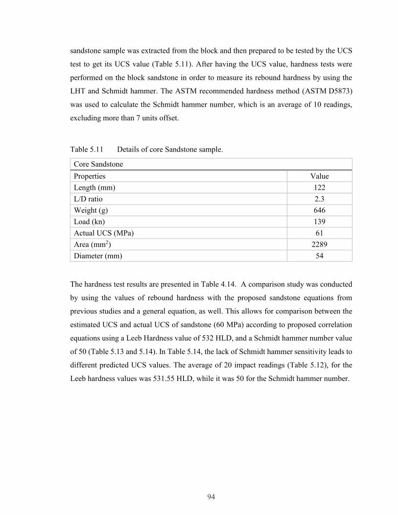
94
sandstone sample was extracted from the block and then prepared to be tested by the UCS
test to get its UCS value (Table 5.11). After having the UCS value, hardness tests were
performed on the block sandstone in order to measure its rebound hardness by using the
LHT and Schmidt hammer. The ASTM recommended hardness method (ASTM D5873)
was used to calculate the Schmidt hammer number, which is an average of 10 readings,
excluding more than 7 units offset.
Table 5.11 Details of core Sandstone sample.
Core Sandstone
Properties Value
Length (mm) 122
L/D ratio 2.3
Weight (g) 646
Load (kn) 139
Actual UCS (MPa) 61
Area (mm2) 2289
Diameter (mm) 54
The hardness test results are presented in Table 4.14. A comparison study was conducted
by using the values of rebound hardness with the proposed sandstone equations from
previous studies and a general equation, as well. This allows for comparison between the
estimated UCS and actual UCS of sandstone (60 MPa) according to proposed correlation
equations using a Leeb Hardness value of 532 HLD, and a Schmidt hammer number value
of 50 (Table 5.13 and 5.14). In Table 5.14, the lack of Schmidt hammer sensitivity leads to
different predicted UCS values. The average of 20 impact readings (Table 5.12), for the
Leeb hardness values was 531.55 HLD, while it was 50 for the Schmidt hammer number.

95
Table 5.12 Rebound Hardness values of Leeb Hardness Test (HLD) and Schmidt
Hammer Test (R) on Sandstone Block.
HLD R
566 44
487 46
530 48
535 50
523 52
554 48
523 50
544 54
556 46
524 50
488 48
530 52
570 50
526 54
481 50
530 52
560 48
528 54
530 52
546 52
Table 5.13 Comparison between estimated UCS and actual UCS of sandstone (60
MPa) using the proposed correlation equations in this study.
Estimated
UCS (MPa)
UCS Equation with
“HLD” value
Researcher R Lithology
49 UCS= 9E-07HLD 2.839 Present Study, 2016 0.72 Sandstone
57.5 UCS= 6.72E-07 *
HLD2.91
Present Study, 2016 0.7 Sedimentary
61.64 UCS= 1.57E-05HLD 2.419 Present Study, 2016 0.7 Varied
52 UCS= 8*10-6*HLD 2.5 Aoki &Matsukura,
2008
0.77 Varied

96
Table 5.14. Comparison between estimated UCS and actual UCS of Sandstone (60
MPa) according to proposed correlation equations using Leeb Hardness
value of 532 HLD, and Schmidt hammer number (R) of 50.2. The ASTM
standard method was used to calculate the Schmidt hammer number.
Estimated
UCS (MPa)
UCS Equation with “R”
value
Researcher R Lithology
58.60 UCS =0.308R1.327 Sapporo et al
(2013)
0.9 Sandstone,
mudstone
104.4 UCS = 2R Singh et al (1983) 0.72 Sandstone,
mudstone
63.8 UCS=2.208e0.06R Katz et al. (2000) 0.96 Sandstone,
Limestone
49.5 UCS= 0.994R-0.383 Haramy&DeMarc
o, 1985
0.87 Sedimentary
5.4 Chapter Summary
This study has proposed to develop a correlation between the HLD and UCS by rock types,
which could become a significant application for rock engineering practices. In order to
propose a relationship that can be used in fieldwork, a field evaluation of the potential UCS-
HLD correlation was performed, and a statistical analysis was conducted to analyze the
results. This method provides a convenient means to obtain improved accuracy in the field
estimation of UCS. Statistical measurements on the database were collected from the
literature review and the results of laboratory tests to determine how well the regression
line fits the database. Then, the UCS-HLD correlation was plotted to establish an equation
relating UCS (MPa) and HLD. In addition, the three main rock types were analyzed and
the plot of UCS-HLD correlations were presented.
Collected HLD values were classified based on three rock types, and a link between these
classifications as well as rock strength grades established by ISRM has been proposed, the
degree of uncertainty was also presented. The results of a comparison between two rebound
hardness devices the LHT and Schmidt hammer were presented.

97
CHAPTER 6 CONCLUSION and RECOMMENDATION
Currently there are neither agreement on one prediction model that can predicate the UCS
using LHT nor well-established procedure for LHT in the rock engineering field. Therefore,
this study proposed a correlation of LHD with UCS to fill the gap of the limited precision
and reliability of ISRM field estimate for estimating the strength of intact rocks or other
indexing methods. Moreover, this study aimed to develop an understanding of the
confidence associated with the number of impacts per test and the sample size effect on
hardness values, and aimed to recommend a testing procedure based on the results. This
could be used to appropriately obtain from the field for design purpose.
To get a reasonable measure of the representative hardness of a rock, the LHT methodology
was examined by quantifying the sample size and the number of Leeb impacts. This was
achieved by examining the number of impacts required for a valid test and the effect of
sample size on the measured hardness value. The study proposed that there are minimal
gains for extra tests beyond 10 impact readings to perform the LHT. In the study procedure,
a trimmed mean was used where 12 readings were taken and the highest and lowest values
were removed, and the remaining 10 impacts were averaged in a “test” result. This was
observed to provide a more accurate basis for UCS determination. In addition, a nonlinear
relationship between specimen size and HLD below 100 mm exists; however, results were
relatively constant above 100 mm, indicating that this is the critical specimen length for the
LHT. A small specimen size could be corrected for using the nonlinear relationship.
Moreover, this study provided the scale effect for the mean HLD, normalized by the value
of the standard length of 102 mm, as a function of the specimen length. It has also been
observed that there is an increase in the value of the HLD as the length increases. This study
proposed a relationship for less than L/D=1.5 and the influence of core sample length
(HLDL) related to standardized value (HLD102mm).
The statistical relationship between the HLD and UCS for different rock types was
investigated. That was done by analyzing the points from our lab and other literature from
98
the mining industry partners. Building a database with a total of 311 points helped to
establish how accurately the UCS of rock material could be obtained by using a portable
LHT. Utilizing HLD-UCS database, this study has presented a nonlinear relation between
HLD and UCS for improved accuracy in field estimation of UCS.
Analysis was conducted on the three main rock types (igneous, metamorphic and
sedimentary), collected from a literature review and the results of our laboratory study. The
results of a comparison between LHT and Schmidt Hammer show that even though these
rock specimens are from the same designation of rocks (igneous), there is considerable
scatter between the UCS values for each specimen. The shapes of the UCS-HLD curves
were similar in each rock types. The best-fit regression lines were plotted for the UCS-HLD
correlation of all rock type and the correlation equations of all three rock types were
presented with suitable R2 and S value.
Generally, there is an increase in UCS with increasing HLD, despite the fact that the
specimens used to develop the relationship were differentiated by formation sites and
weathering. The correlations of sedimentary and metamorphic rocks show lower S value
and higher R2 value than igneous rocks. Due to the durability of igneous rocks when
subjected to a load, they showed high UCS values relative to other rock types.
An improved correlation between HLD and UCS for different rock types was found and its
accuracy was assessed by the lowest S, which is a useful measure to assess the precision of
the predictions of the results of correlation analysis. The value of S of the study was found
to be lower than those that were calculated from other correlation equations, whereas S
associated with the correlation model should be as small as possible. That means the
reliability and accuracy of the HLD - UCS relationship of the proposed model in this study
is high.
In summary, the results show that the LHT can be particularly useful for field estimation
of UCS and offer a significant improvement over the field estimation methods outlined by
99
the ISRM (2007). The equations that relate HLD to UCS are simple, practical and accurate
enough to apply in the field. This study will act as an improvement to the UCS-HLD
correlations that were done by other authors.
For future Leeb hardness studies, including the effect of physical properties such as the
effect of the following two efficiency components, 1. the bond between minerals or grains
and 2. their strengths, the effect of a porosity degree, in addition, the effect of an
inhomogeneity in hardness testing is recommended. For future research, the database
would need to be expanded and improved (more rock types, larger range of UCS.) The
LHT could also be considered for evaluation of anisotropic conditions with further
research. Moreover, In the future, efforts could be made to develop a system where the
LHT automatically preforms many tests over a specimen (e.g., core) with one push of the
button. This would provide a systematic profile of readings.
Quantity the level of uncertainty associated with the HLD – UCS estimation could be
done in future work. Especially, related to the ISRM method and the average of
variability in the typical UCS.
100
REFERENCES
Akram, M., & Bakar, M. A. (2016). Correlation between uniaxial compressive strength and
point load index for salt-range rocks. Pakistan Journal of Engineering and Applied
Sciences.
Aoki, H., & Matsukura, Y. (2008). Estimating the unconfined compressive strength of
intact rocks from Equotip hardness. Bulletin of Engineering Geology and the
Environment, 67(1), 23–29.
Aoki, H., & Matsukura, Y. (2007). A new technique for non-destructive field
measurement of rock-surface strength: an application of the Equotip hardness tester
to weathering studies. Earth Surface Processes and Landforms, 32(12), 1759–1769.
Asef, M. R. (1995). Equotip as an index test for rock strength properties (Doctoral
dissertation, M. Sc. Thesis, ITC Delft)
ASTM. D4543-08 (2008). Standard Practices for Preparing Rock Core as Cylindrical Test
Specimens and verifying Conformance to Dimensional and Shape Tolerances. Astm,
1–9. article.
ASTM, a 956-12 (2012). Standard Test Method for Leeb Hardness Testing of Steel
Products. Standards, 1–12.
ASTM, D3967-08 (2008). Standard Test Method for Splitting Tensile Strength of Intact
Rock Core Specimens 1. ASTM International, West Conshohocken, PA, 20–23.
ASTM, D7012–14 (2014). Standard test method for compressive strength and elastic
moduli of intact rock core specimens under varying states of stress and temperatures,
ASTM International, West Conshohocken, Pa., doi, 10.
ASTM D5873-05 (2005). Standard Test Method for Determination of Rock Hardness by
Rebound Hammer Method, ASTM International, West Conshohocken, PA, 2005.
Aydin, A., & Basu, A. (2005). The Schmidt hammer in rock material characterization.
Engineering Geology, 81(1), 1–14.
Aydin, A. (2015). The ISRM Suggested Methods for Rock Characterization, Testing and
Monitoring: 2007-2014. (R. Ulusay, Ed.). Cham: Springer International Publishing.
101
Basu, A., & Aydin, A. (2004). A method for normalization of Schmidt hammer rebound
values. International Journal of Rock Mechanics and Mining Sciences, 41(7), 1211–
1214.
Bell, F. G. (Ed.). (2013). Engineering in rock masses. Elsevier.
Bieniawski, Z. T. (1975). Estimating the strength of rock materials. Journal of the South
African Institute of Mining and Metallurgy, March, 312–320.
Broch EM, Franklin JA (1972) The point load strength test. Int J Rock Mech Min Sci
Geomech Abstr 9:669–697
BS 5930 (1981). Code of Practice for Site Investigations. British Standards Institution
(BSI). London. 147 pp.
Burnett A.D. (1975). Engineering geology and site investigation - part 2: field studies.
Ground engineering. July. pp. 29 - 32.
Buyuksagis, I. S., & Goktan, R. M. (2007). The effect of Schmidt hammer type on
uniaxial compressive strength prediction of rock. International Journal of Rock
Mechanics and Mining Sciences, 44(2), 299–307.
Cargill JS, Shakoor A. (1990). Evaluation of empirical methods for measuring the
uniaxial compressive strength of rock. Int J Rock Mech Min Sci Geomech Abstr
1990;27(6):495–503.
Coombes, M. A., Feal-Pérez, A., Naylor, L. A., & Wilhelm, K. (2013). A non-destructive
tool for detecting changes in the hardness of engineering materials: Application of
the Equotip durometer in the coastal zone. Engineering Geology, 167, 14-19.
Corkum, a. G., & Martin, C. D. (2007). The mechanical behaviour of weak mudstone
(Opalinus Clay) at low stresses. International Journal of Rock Mechanics and
Mining Sciences, 44, 196–209.
D. Leeb. (1986). Definition of the hardness value "L" in the EQUOTIP dynamic
measuring method?, VDI-Report No. 583, pp. 109-133
D. Leeb. (1990). Dynamische Härteprüfung, in Härteprüfung an Metallen und
Kunststoffen, eds. W.W. Weiler, D.H. Leeb, K. Müller and D.M. Rupp., 2nd
Edition, Expert Verlag, Ehningen bei Böblingen
Daniels, G., Mcphee, C., Sorrentino, Y., & McCurdy, P. (2012). Non-Destructive
Strength Index Testing Applications for Sand Failure Evaluation. Proceedings of
SPE Asia Pacific Oil and Gas Conference and Exhibition, (L), 1–12.
102
Demirdag, S., Yavuz, H., & Altindag, R. (2009). The effect of sample size on Schmidt
rebound hardness value of rocks. International Journal of Rock Mechanics and
Mining Sciences, 46(4), 725–730.
Dynamic, P., & Tester, H. (n.d.). Impact th-170 series portable dynamic hardness tester
portable hardness tester, 170–173
Eassa, A., Staff, F., & Engineer, F. E. R. (2005). Practical Approach Towards Enhanced
Accuracy.
Frank, S., & Schubert, H. (2002). Portable hardness testing- principles and
applications. Journal of Nondestructive Testing, 7(10), 8
Gorski, B., Anderson, T., Rodgers, D., Rogers, D., Raven, K., Mccreath, D., & Lam, T.
(2010). Supplementary Uniaxial Compressive Strength Testing of DGR-3 and DGR-
4 Core.
Goudie, A. S. (2013). The Schmidt Hammer and Related Devices in Geomorphological
Research. In Treatise on Geomorphology (Vol. 14, pp. 338–345).
Grima, M. A., & Babusï, R. (1999). Fuzzy Model for The Prediction of Unconfined
Compressive Strength of Rock Specimens. International Journal of Rock Mechanics
and Mining Sciences, 36, 339–349.
Guerra, E., de Lara, J., Malizia, A., & Díaz, P. (2009). Supporting user-oriented analysis
for multi-view domain-specific visual languages. Information and Software
Technology.
Hack, H., Hingira, J., & Verwaal, W. (1993). Determination of discontinuity wall strength
by Equotip and ball rebound tests. International Journal of Rock Mechanics and
Mining Sciences & Geomechanics Abstracts, 30(2), 151–155.
Hack, R., & Huisman, M. (2002). Estimating the intact rock strength of a rock mass by
simple means. Engineering Geology for Developing Countries, (0), 1971–1977.
Hawkins AB (1998) Aspects of rock strength. Bull Eng Geol Env 57:17–30
Hawkins AB, Olver JAG (1986) Point load tests: correlation factor and contractual use.
An example from the Corallian at Weymouth In: Hawkins AB (ed) Site Investigation
Practice: Assessing BS 5930, Geological Society, London, pp 269–271
Hoek, E., & Martin, C. D. (2014). Fracture initiation and propagation in intact rock – A
review. Journal of Rock Mechanics and Geotechnical Engineering, 6(4), 287–300.
JOUR.

103
Houston, M., & Long, F. (2004). Correlations Between Different Its and Ucs Test
Protocols for Foamed Bitumen Treated Materials, (September), 522–536.
Hoek E, Brown ET (1980) Underground excavations in rock. Inst Min Metal, London
Hucka, V. (1965). A rapid method of determining the strength of rocks in situ.
In International Journal of Rock Mechanics and Mining Sciences & Geomechanics
Abstracts (Vol. 2, No. 2, pp. 127IN3131-130IN6134). Pergamon.
Hudson, J. A. (1993). Comprehensive rock engineering: principles, practice, and
projects. Book, Pergamon Press.
Hujer, W. H., Finkbeiner, T., & Persaud, M. (2014). Estimating Rock Strength From
Non-Destructive Strength Testing (EQUOTIP) and Related Benefits.
Hujer, W. H., Finkbeiner, T., & Persaud, M. (2014). Estimating Rock Strength From
Non-Destructive Strength Testing (EQUOTIP) and Related Benefits.
ISRM. International Society of Rock Mechanics Commission on Testing Methods,
Suggested Method for Determining Point Load Strength, Int. J. Rock Mech. Min.
Sci. and Geomech. Abstr. 22, 1985, pp.51-60.
ISRM. (1979). Suggested methods for determining the uniaxial compressive strength and
deformability of rock materials. International Journal of Rock Mechanics & Mining
Sciences, 16(December), 135–140.
Jonatan, P. (2015). UCS test Sample Preparation: A Guide. Department of Civil and
Resource Engineering, Dalhousie University.
Kahraman, S. (2001). Evaluation of simple methods for assessing the uniaxial
compressive strength of rock. Rock Mechanics, 38, 981–994.
Kahraman, S., Fener, M., & Gunaydin, O. (2004). Predicting the sawability of carbonate
rocks using multiple curvilinear regression analysis. International Journal of Rock
Mechanics and Mining Sciences, 41(7), 1123–1131.
Kallu, R., & Roghanchi, P. (2015). Correlations between direct and indirect strength test
methods. International Journal of Mining Science and Technology, 25(3), 355–360.
Karakus, M., Kumral, M., & Kilic, O. (2005). Predicting elastic properties of intact rocks
from index tests using multiple regression modelling. International Journal of Rock
Mechanics and Mining Sciences, 42(2), 323-330.
Karaman, K., & Kesimal, A. (2014). Correlation of Schmidt Rebound Hardness with
Uniaxial Compressive Strength and P-Wave Velocity of Rock Materials. Arab J Sci
Eng, 40, 1897–1906.

104
Karpuz, C. (1990). A classification system for excavation of surface coal
measures. Mining Science and Technology, 11(2), 157-163.
Katz, O., Reches, Z., & Roegiers, J. C. (2000). Evaluation of mechanical rock properties
using a Schmidt Hammer. International Journal of Rock Mechanics and Mining
Sciences, 37(4), 723–728.
Kawasaki, S., Tanimoto, C., Koizumi, K., & Ishikawa, M. (2002). An attempt to estimate
mechanical properties of rocks using the Equotip hardness tester. Journal of the
Japan Society of Engineering Geology, 43(4), 244-248.
Kawasaki, S., & Kaneko, K. (2004). Estimation method for weathering thickness of man-
made weathering rocks by using the Equotip hardness tester. In Proc. ISRM
Regional Symp. EUROROCK (pp. 491-494).
Kompatscher, M. (2004). Equotip-rebound hardness testing after D. Leeb. Proceedings,
Conference on Hardness Measurements, 1975. Retrieved from
http://www.imeko.org/publications/tc5-2004/IMEKO-TC5-2004-014.pdf
Landau, L. (1937). Method for Determining the Unconfined Compressive Strength of
Intact Rock Core Specimens SC T 39. Zhurnal Eksperimental’noi I Teoreticheskoi
Fiziki, 1–4. Retrieved from
Lee, J. S., Smallwood, L., & Morgan, E. (2014, A. (2014). New Application of Rebound
Hardness Numbers to generate Logging of Unconfined Compressive Strength in
Laminated Shale Formations. New Application of Rebound Hardness Numbers to
Generate Logging of Unconfined Compressive Strength in Laminated Shale
Formations.
Li, D., & Wong, L. N. Y. (2013). Point Load Test on Meta-Sedimentary Rocks and
Correlation to UCS and BTS. Rock Mechanics and Rock Engineering, 46(4), 889–
896.
Luppi, L., Rinaldi, M., Teruggi, L. B., Darby, S. E., & Nardi, L. (2009). Monitoring and
numerical modelling of riverbank erosion processes: a case study along the Cecina
River (central Italy), 1769, 1759–1769.
Meulenkamp, F., & Grima, M. A. (1999). Application of neural networks for the
prediction of the unconfined compressive strength (UCS) from Equotip hardness.
International Journal of Rock Mechanics and Mining Sciences, 36.
Mol, L. (2014). Measuring rock hardness in the field. British Society for Geomorphology
Geomorphological Techniques, 32(1).
Momeni, E., Nazir, R., Armaghani, D. J., For, M., Amin, M., & Mohamad, E. T. (2015).
Prediction of unconfined compressive strength of rocks : a review paper, 11, 43–50.

105
Palchik V, Hatzor YH (2004) The influence of porosity on tensile and compressive
strength of porous chalks. Rock Mech Rock Eng 37(4):331–341
Proceq SA (1977a) Operating instructions concrete test hammer types N and NR. Zurich,
Switzerland.
Proceq SA (1977b) Equotip operations instructions, 5th edn. PROCEQ SA Zurich,
Switzerland
Pycnometer, W., Soil, T., & Limit, P. (2007). Standard Test Method for Unconfined
Compressive Strength of Cohesive Soil 1, 3(Reapproved 2002), 1–6.
Rodríguez-Rellán, C., Valcarce, R. F., & Esnaola, E. B. (2011). Shooting out the slate:
Working with flaked arrowheads made on thin-layered rocks. Journal of
Archaeological Science, 38(8), 1939–1948.
Romana M (1999). Correlation between uniaxial compressive and point load (Franklin
test) strengths for different rock classes. In: 9th ISRM Congress, 1999, vol 1, pp
673–676, Paris
Rusakov, N. G., & Mavrodi, P. I. (N.D.). Determination of The Strength Of Rock By The
Impact Method.
Ryan, T. A., Joiner, B. L., & Ryan, B. F. (2004). Minitab™. John Wiley & Sons, Inc
Selçuk, L., & Yabalak, E. (2015). Evaluation of the ratio between uniaxial compressive
strength and Schmidt hammer rebound number and its effectiveness in predicting
rock strength. Nondestructive Testing and Evaluation, 30(1), 1–12.
Sheskin, D. J. (2000). Parametric and nonparametric statistical procedures. Boca Raton:
CRC.
Sjoberg, J. (1997). Estimating rock mass strength using Hoek-Brown failure criterion and
rock mass classification, 61.
Stefan, F. (2003). Mobile hardness testing. Insight, 45(9), 651
Szilágyi, K. (2012). Hardness studies on porous solids. In Conference of Junior
Researchers in Civil Engineering (pp. 240–247).
Szilágyi, K. (2013). Rebound surface hardness and related properties of concete, 439.
Szwedzicki, T. (1998). Technical note Indentation Hardness Testing of Rock, 35(6), 825–
829.

106
Thuro K, Plinninger RJ (2005) Scale effects in rock properties: Part 2. Point load test and
point load strength index. EUROCK Swets and Zeitlinger, pp 175–180, Lisse
Torabi, S. R., Ataei, M., & Javanshir, M. (2011). Application of Schmidt rebound number
for estimating rock strength under specific geological conditions. Journal of Mining
and Environment, 1(2), 1–8.
Tsiambaos G, Sabatakakis N (2004) Considerations on strength of intact sedimentary
rocks. Eng Geol 72:261–273
Van de Wall, I. A. R. G., & Ajalu Msc, J. S. (1997). Characterization of the geotechnical
properties of rock material for construction purposes. International Journal of Rock
Mechanics and Mining Sciences, 34(3–4), 319.e1-319.e12.
Verwaal, W., & Mulder, A. (1993). Estimating rock strength with the Equotip hardness
tester. International Journal of Rock Mechanics and Mining Sciences &
Geomechanics Abstracts, 30, 659–662. http://doi.org/10.1016/0148-9062(93)91226-
9
Verwall, W., & Mulder, A. (2000). Rock and aggregate test procedures. Rock and
aggregate laboratory manual, 13, 14.
Viles, H., Goudie, A., Grab, S., & Lalley, J. (2011). The use of the Schmidt Hammer and
Equotip for rock hardness assessment in geomorphology and heritage science: A
comparative analysis. Earth Surface Processes and Landforms, 36(July 2010), 320–
333.
Yaşar, E., & Erdoǧan, Y. (2004). Estimation of rock physicomechanical properties using
hardness methods. Engineering Geology, 71(3–4), 281–288.
Yilmaz, N. G. (2013). The influence of testing procedures on uniaxial compressive
strength prediction of carbonate rocks from Equotip hardness tester (EHT) and
proposal of a new testing methodology: Hybrid dynamic hardness (HDH). Rock
Mechanics and Rock Engineering, 46(1), 95–106.
Zhang, Q., Zhu, H., Zhang, L., & Ding, X. (2011). Study of scale effect on intact rock
strength using particle flow modeling. International Journal of Rock Mechanics and
Mining Sciences, 48(8), 1320–1328.

107
Appendix 1
CONFERENCE PAPER
Leeb Hardness Test for UCS estimation of Sandstone
Yassir Asiri, Andrew Corkum & Hany El Naggar
Department of Civil and Resource Engineering
ABSTRACT
An experimental exploration has been conducted to investigate the statistical relationship
between Leeb Hardness (“D” type) values (HLD) and unconfined compressive strength
values (UCS) for sandstone. Moreover, the Leeb test methodology was evaluated, such as
sample size and the number of Leeb readings that comprise a valid test result. The
laboratory testing was carried out on sandstone specimens and combined with other
literature values to develop a database with a total of 45 test results. Statistical analysis was
carried out on the database and the results of correlation analysis from tests are presented.
A reasonable correlation was found to exist between LHD and UCS for sandstone. The
results show that the Leeb Hardness test (LHT) can be particularly useful for field
estimation of UCS. The method is fast, simple and equipment costs are low. The hardness
testing cannot replace UCS tests but can complement these tests, especially if is needed
immediately or other testing is not possible.
108
RÉSUMÉ
Une exploration expérimentale a été menée pour étudier la relation statistique entre Leeb
Dureté (type « D ») des valeurs (HLD) et des valeurs de résistance à la compression
uniaxiale (UCS) pour la roche. En outre, la méthodologie de test Leeb a été évaluée, comme
la taille de l'échantillon et le nombre de lectures Leeb qui comprennent un résultat de test
valide. Les tests de laboratoire ont été effectués sur des échantillons de grès et combiné
avec d'autres valeurs de la littérature pour développer une base de données avec un total de
45 résultats. L'analyse statistique a été réalisée sur la base de données et les résultats de
l'analyse de corrélation des essais sont présentés. Une corrélation raisonnable existe entre
LHD et UCS pour le grès. Les résultats montrent que le test de dureté Leeb peut être
particulièrement utile pour l'estimation du champ de UCS. La méthode est simple, rapide
et les coûts d'équipement sont faibles. L'essai de dureté ne peut pas remplacer les tests UCS
mais peut compléter ces tests, en particulier si les données sont nécessaires immédiatement
ou autres tests n’est pas possible.
109
1 INTRODUCTION
The unconfined compressive strength (UCS) of rock is a very important parameter for rock
classification, rock engineering design and numerical modeling. In addition, this property
is essential for judgment about the rocks suitability for various construction purposes.
However, determination of rock UCS is relatively time consuming and expensive for many
projects. Consequently, the use of a portable, fast and cost effective index test that can
reasonably estimate UCS would be desirable. Other index tests, such as the Schmidt
hammer and Point Load Test are commonly used for this purpose. However, this work
looked at the LHT, which is quick, inexpensive and nondestructive: particularly valuable
at preliminary project stages.
The LHT method was introduced in 1975 by Dietmar Leeb at Proceq SA (Kompatscher,
2004). The LHT is a portable hardness tester originally for measuring the strength of
metallic materials. Recently, it has been applied to various rocks for testing their hardness
(e.g. Aoki and Matsukura, 2007; Viles et al., 2011), it can also be correlated with rock UCS
according to Kawasaki et al., 2002; Aoki and Matsukura, 2007. Moreover, it is used to
assess the weathering effects on hardness values (Kawasaki and Kaneko, 2004; Aoki and
Matsukura, 2007; Viles et al., 2011). The LHT can be used in laboratory or the field at any
angle (Viles et al., 2011), since the instrument uses automatic compensation for impact
direction. It is suitable for applications to cover a wider range of most rock hardness
compared with the Schmidt hammer (Aoki and Matsukura 2007).
The aim of this study is to investigate the statistical relationship between Leeb Hardness
(“D” type) values (HLD) and UCS for sandstone, which is one of most uniform and
consistent rocks. For this reason, the laboratory testing was carried out on sandstone and
combined with other literature values to develop a database with a total of 45 test results.
the LHT methodology was evaluated (sample size and the number of Leeb readings that
comprise an average test result). Statistical analysis was carried out on the database and the
results of correlation analysis from tests are presented. Reasonable correlations between
LHD and UCS for sandstone were developed and their accuracy was assessed. The results
show that the LHT can be particularly useful for field estimation of UCS and offer a
significant improvement over the field estimation methods outlined by the ISRM (2007).
The equations that relate HLD to UCS are simple, practical and accurate enough to apply.
110
The method is fast, simple and equipment costs are low. Although the empirically rock
strength predicted from the in-direct LHT results contain some level of uncertainty, but are
of significant value for preliminary design. Moreover, it could be used on core to provide
a continuous profile of estimated UCS in a borehole log with minimal effort for UCS even
beyond the preliminary engineering stage
2 Backgrounds
The LHT can determine the mechanical hardness without destruction of specimens, which
in turn reduces cost and simplifies processes. It has been used widely in rock mechanics
research due to its simplicity. In 1993, Verwaal and Mulder at Delft University of
Technology, examined the possibility of predicting the UCS from HLD value. They
presented the UCS versus HLD relationship and the influence of the surface roughness on
the LHT measurement. Also, they stated that, provided the specimens have a thickness of
greater than 50 mm, the sample thickness has slight effect on the LHT measurement. They
ended with a simple equation for estimating UCS from the measurements of LHT.
Additionally, Hack et al. (1993) used both LHT and ball rebound tests to describe the UCS
of the discontinuity plane for mixed lithologies of various rock type specimens. They
attempted to find the relationship between UCS and Equotip L-values or rebound values of
the ball test and estimate the mechanical strength of the rock surface along a discontinuity
using the Verwaal and Mulder equation.
In 1999 Meulenkamp and Grima used a neural network to predict the UCS from HLD and
several other rock characteristics (porosity, density, grain size and rock type) as input.
However, this is a complex approach and required many input parameters, each of which
added complexity and additional uncertainty to the method. This removed the “simplicity”
of the test and it restricted their approach to the availability and quality of the secondary
inputs. Moreover, the proposed equation includes many variables, which in turn is not
practical in field estimation. Finally, to the author’s knowledge, the neural network
algorithm details were not published and made readily available.
Okawa et al. (1999) tested the effects of the measurement conditions on the rebound value
and concluded that the rebound value depends partially on specimen support (i.e., physical
constraint). In addition, multiple tests on the exact same location tend to increase the local
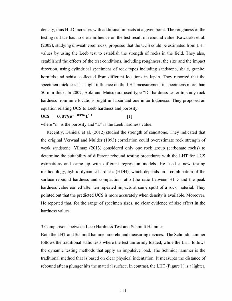
111
density, thus HLD increases with additional impacts at a given point. The roughness of the
testing surface has no clear influence on the test result of rebound value. Kawasaki et al.
(2002), studying unweathered rocks, proposed that the UCS could be estimated from LHT
values by using the Leeb test to establish the strength of rocks in the field. They also,
established the effects of the test conditions, including roughness, the size and the impact
direction, using cylindrical specimens of rock types including sandstone, shale, granite,
hornfels and schist, collected from different locations in Japan. They reported that the
specimen thickness has slight influence on the LHT measurement in specimens more than
50 mm thick. In 2007, Aoki and Matsukura used type “D” hardness tester to study rock
hardness from nine locations, eight in Japan and one in an Indonesia. They proposed an
equation relating UCS to Leeb hardness and porosity:
𝐔𝐂𝐒 = 𝟎. 𝟎𝟕𝟗𝐞−𝟎.𝟎𝟑𝟗𝐧 𝐋𝟏.𝟏 [1]
where “n” is the porosity and “L” is the Leeb hardness value.
Recently, Daniels, et al. (2012) studied the strength of sandstone. They indicated that
the original Verwaal and Mulder (1993) correlation could overestimate rock strength of
weak sandstone. Yilmaz (2013) considered only one rock group (carbonate rocks) to
determine the suitability of different rebound testing procedures with the LHT for UCS
estimations and came up with different regression models. He used a new testing
methodology, hybrid dynamic hardness (HDH), which depends on a combination of the
surface rebound hardness and compaction ratio (the ratio between HLD and the peak
hardness value earned after ten repeated impacts at same spot) of a rock material. They
pointed out that the predicted UCS is more accurately when density is available. Moreover,
He reported that, for the range of specimen sizes, no clear evidence of size effect in the
hardness values.
3 Comparisons between Leeb Hardness Test and Schmidt Hammer
Both the LHT and Schmidt hammer are rebound measuring devices. The Schmidt hammer
follows the traditional static tests where the test uniformly loaded, while the LHT follows
the dynamic testing methods that apply an impulsive load. The Schmidt hammer is the
traditional method that is based on clear physical indentation. It measures the distance of
rebound after a plunger hits the material surface. In contrast, the LHT (Figure 1) is a lighter,

112
smaller and non-destructiveness device that leaves a little damage with an indentation of
just ~0.5 mm, which is good for a thin layer. LHT is also faster, a test takes a mere “2”
seconds. Thus for practical purposes, speed, size and weight of the LHT make it easier to
deal with in the field.
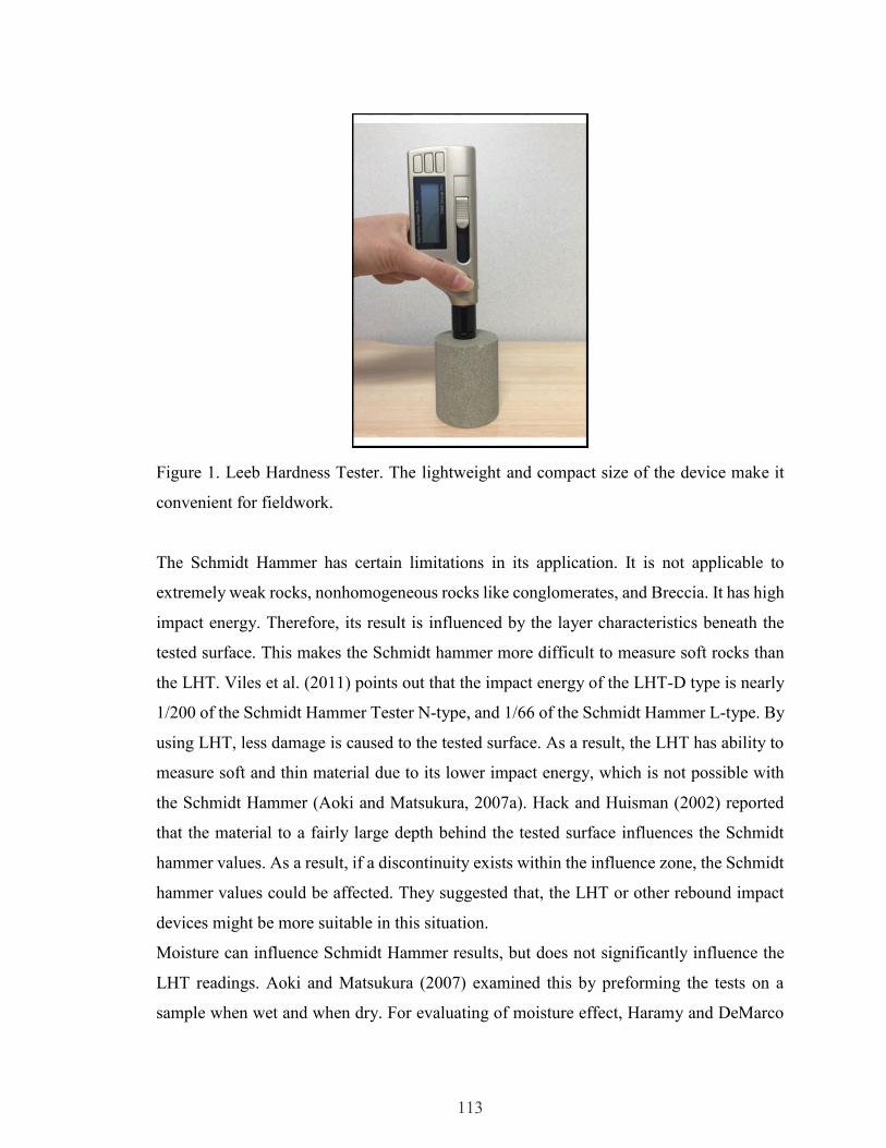
113
Figure 1. Leeb Hardness Tester. The lightweight and compact size of the device make it
convenient for fieldwork.
The Schmidt Hammer has certain limitations in its application. It is not applicable to
extremely weak rocks, nonhomogeneous rocks like conglomerates, and Breccia. It has high
impact energy. Therefore, its result is influenced by the layer characteristics beneath the
tested surface. This makes the Schmidt hammer more difficult to measure soft rocks than
the LHT. Viles et al. (2011) points out that the impact energy of the LHT-D type is nearly
1/200 of the Schmidt Hammer Tester N-type, and 1/66 of the Schmidt Hammer L-type. By
using LHT, less damage is caused to the tested surface. As a result, the LHT has ability to
measure soft and thin material due to its lower impact energy, which is not possible with
the Schmidt Hammer (Aoki and Matsukura, 2007a). Hack and Huisman (2002) reported
that the material to a fairly large depth behind the tested surface influences the Schmidt
hammer values. As a result, if a discontinuity exists within the influence zone, the Schmidt
hammer values could be affected. They suggested that, the LHT or other rebound impact
devices might be more suitable in this situation.
Moisture can influence Schmidt Hammer results, but does not significantly influence the
LHT readings. Aoki and Matsukura (2007) examined this by preforming the tests on a
sample when wet and when dry. For evaluating of moisture effect, Haramy and DeMarco

114
(1985), reported that Schmidt’s is affected by water content of the surface in addition to the
roughness of the surface area, rock strength, cleavage and pores as well. The LHT device
is sensitive to surface conditions, so it cannot be used successfully on friable or rough
surfaces of rocks.
The LHT has the ability to repeat the impact test on the same sample even on the same
spot without breaking the sample, which is not always possible with Schmidt hammer
(Aoki and Matsukura, 2007a). This allows the LHT to be used on small specimens or on
those of limited thickness. In the laboratory both devices require the specimens to be well
clamped in order to avoid any movement.
The Schmidt Hammer is less sensitive to localized conditions at the impact location
making reading more consistent and representing the average rock properties. The LHT is
more precise (smaller area) and therefore is affected by local mineralogy and geometry.
Doing multiple Leeb readings and averaging them for a single “test” reading can alleviate
this. LHT has certain advantages such as the smaller diameter of its tip (3 mm), which
means greater accuracy of its measurement, also the automatic correction of the angle,
which minimizes the variations in measurements produced by the gravity force. In addition,
the LHT can be used either in laboratory or the field, because of portability, simplicity, low
cost, its speed and non-destructiveness. Also, it positions at any angle and either straight or
curved surface while Schmidt’s direction is restricted.
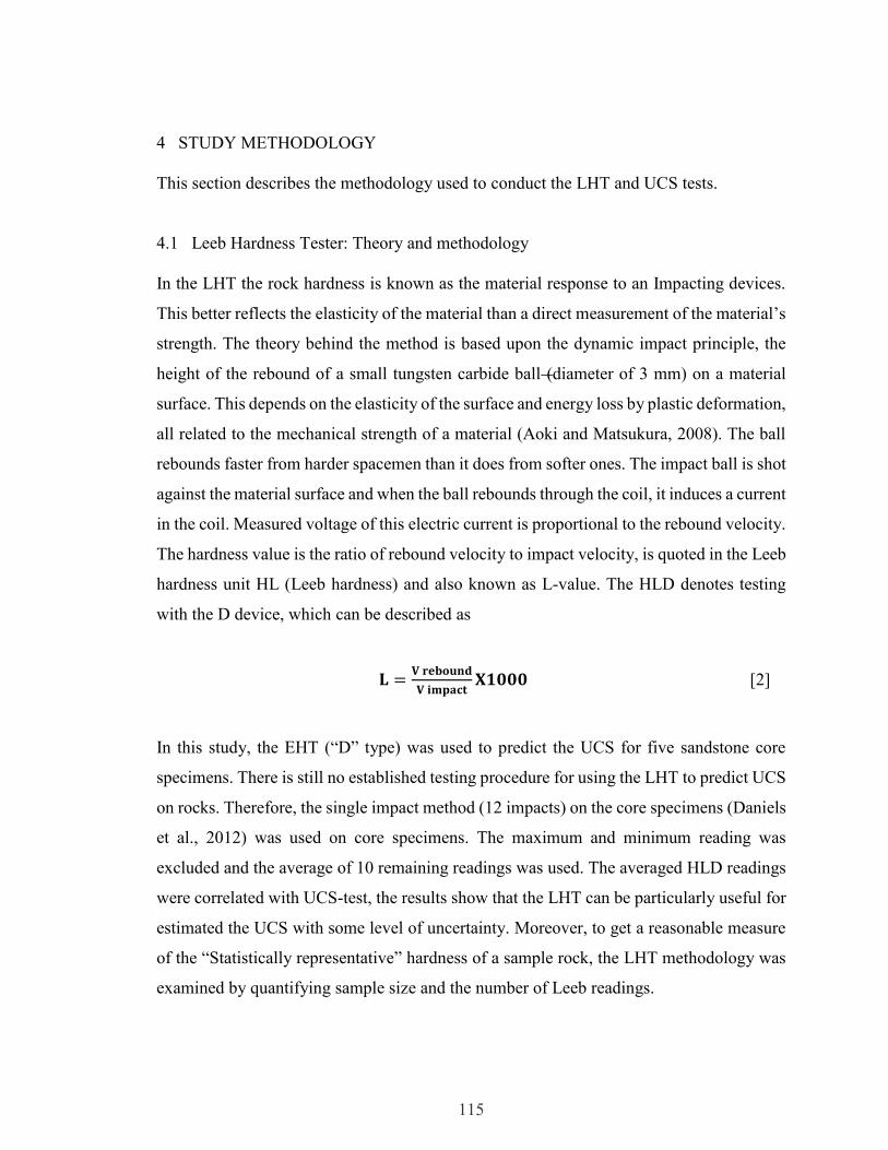
115
4 STUDY METHODOLOGY
This section describes the methodology used to conduct the LHT and UCS tests.
4.1 Leeb Hardness Tester: Theory and methodology
In the LHT the rock hardness is known as the material response to an Impacting devices.
This better reflects the elasticity of the material than a direct measurement of the material’s
strength. The theory behind the method is based upon the dynamic impact principle, the
height of the rebound of a small tungsten carbide ball (diameter of 3 mm) on a material
surface. This depends on the elasticity of the surface and energy loss by plastic deformation,
all related to the mechanical strength of a material (Aoki and Matsukura, 2008). The ball
rebounds faster from harder spacemen than it does from softer ones. The impact ball is shot
against the material surface and when the ball rebounds through the coil, it induces a current
in the coil. Measured voltage of this electric current is proportional to the rebound velocity.
The hardness value is the ratio of rebound velocity to impact velocity, is quoted in the Leeb
hardness unit HL (Leeb hardness) and also known as L-value. The HLD denotes testing
with the D device, which can be described as
𝐋 =𝐕 𝐫𝐞𝐛𝐨𝐮𝐧𝐝
𝐕 𝐢𝐦𝐩𝐚𝐜𝐭𝐗𝟏𝟎𝟎𝟎 [2]
In this study, the EHT (“D” type) was used to predict the UCS for five sandstone core
specimens. There is still no established testing procedure for using the LHT to predict UCS
on rocks. Therefore, the single impact method (12 impacts) on the core specimens (Daniels
et al., 2012) was used on core specimens. The maximum and minimum reading was
excluded and the average of 10 remaining readings was used. The averaged HLD readings
were correlated with UCS-test, the results show that the LHT can be particularly useful for
estimated the UCS with some level of uncertainty. Moreover, to get a reasonable measure
of the “Statistically representative” hardness of a sample rock, the LHT methodology was
examined by quantifying sample size and the number of Leeb readings.
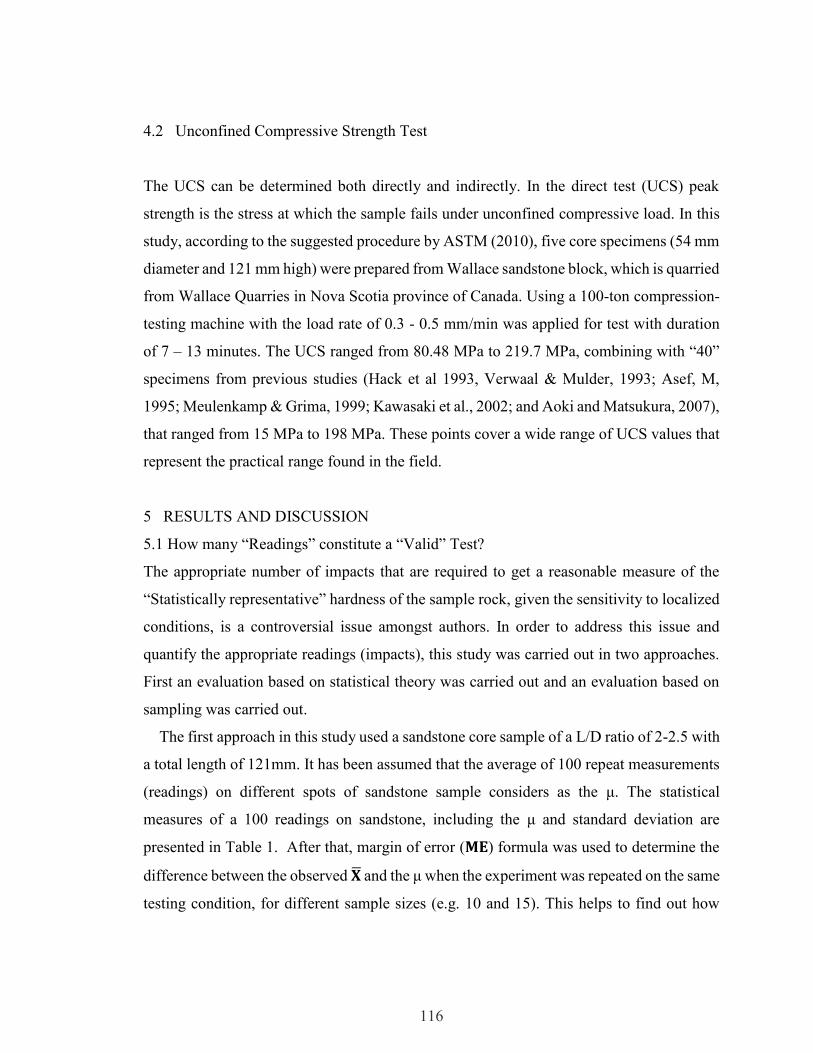
116
4.2 Unconfined Compressive Strength Test
The UCS can be determined both directly and indirectly. In the direct test (UCS) peak
strength is the stress at which the sample fails under unconfined compressive load. In this
study, according to the suggested procedure by ASTM (2010), five core specimens (54 mm
diameter and 121 mm high) were prepared from Wallace sandstone block, which is quarried
from Wallace Quarries in Nova Scotia province of Canada. Using a 100-ton compression-
testing machine with the load rate of 0.3 - 0.5 mm/min was applied for test with duration
of 7 – 13 minutes. The UCS ranged from 80.48 MPa to 219.7 MPa, combining with “40”
specimens from previous studies (Hack et al 1993, Verwaal & Mulder, 1993; Asef, M,
1995; Meulenkamp & Grima, 1999; Kawasaki et al., 2002; and Aoki and Matsukura, 2007),
that ranged from 15 MPa to 198 MPa. These points cover a wide range of UCS values that
represent the practical range found in the field.
5 RESULTS AND DISCUSSION
5.1 How many “Readings” constitute a “Valid” Test?
The appropriate number of impacts that are required to get a reasonable measure of the
“Statistically representative” hardness of the sample rock, given the sensitivity to localized
conditions, is a controversial issue amongst authors. In order to address this issue and
quantify the appropriate readings (impacts), this study was carried out in two approaches.
First an evaluation based on statistical theory was carried out and an evaluation based on
sampling was carried out.
The first approach in this study used a sandstone core sample of a L/D ratio of 2-2.5 with
a total length of 121mm. It has been assumed that the average of 100 repeat measurements
(readings) on different spots of sandstone sample considers as the μ. The statistical
measures of a 100 readings on sandstone, including the μ and standard deviation are
presented in Table 1. After that, margin of error (𝐌𝐄) formula was used to determine the
difference between the observed �̅� and the μ when the experiment was repeated on the same
testing condition, for different sample sizes (e.g. 10 and 15). This helps to find out how
117
many impacts we would need to get a �̅� which is almost equal to the population mean,
based on 100 readings with a degree of confidence interval of 95%.
We can quantity the precise of our �̅�, for sample sizes less than 100, by using ME. The
relation between population mean and �̅� can calculate using:
𝛍 = �̅� ± 𝟏. 𝟗𝟔 (𝛔
√𝐧 ) [3]
where μ is the population mean,1.96 is the critical Z value of the standard normal
distribution at a 95% degree of confidence, σ is the standard deviation of the population, n
is the sample size and �̅� is the sample mean. The formula to establish the margin of error
at different sample sizes (e.g. at 10 and 15) is:
𝐌𝐄 = 𝟏. 𝟗𝟔 (𝛔
√𝐧 )
[4]
The results using the sandstone sample, for which we have 100 repeated measurements are
shown in Table 2. Table 2 illustrates that, in general, LHT require much more sampling
effort to obtain a good estimate of the true hardness on rocks.
The second approach is based on sampling, relying on the Central Limit Theorem and
the Law of Large Numbers. The key idea in the Central Limit Theorem is that when a
population is repeatedly sampled, the calculated average value of the feature obtained by
those specimens is equal to the true population mean value, and the Law of Large Numbers
states that as a sample size grows, its mean will converge in probability towards the average
of the whole population. Accordingly, this study was performed on a total of 100 readings
(impacts) on a sandstone core sample of a L/D ratio of 2-2.5 with a total length of 121mm.
Once this population set (100 readings) was captured, a subset number of readings (e.g.,
10, 15, 20, 30) were randomly selected, to ensure that all of the points are being well
represented taking into consideration all different aspects to avoid being biased by the
performer, and the mean value was determined. This was done on with subset sizes ranging

118
from 1 to 100 readings. Moreover, because of the high variability of �̅� at low sample
numbers, a total of five “realizations” of this randomized subset study were carried out.
This helps to visually assess how many impacts we would need to get a �̅� which is
almost equal to the population mean, based on 100 readings with a degree compared to the
confidence interval. A graph was then plotted representing the with the average of readings
that was previously calculated on the Y-axis against the number of tries, which was a 100
on the X- axis (Figure 2). This method graphically shows that by increasing the number of
averaged, their arithmetic mean gets close to the 100 readings mean (population mean).
Moreover, this graph helps determine the minimum number of readings required to carry
out a 'Valid' test based on the standard deviation rules and visually assess the error
associated with limited sample size (e.g. 10 readings). As shown in Figure 2, it is clear that
there are minimal gains for extra tests beyond 10 in sandstone.
5.2 Evaluation of Sample Size and Scale Effects
It has been observed in several studies that there is a correlation between the scale effects
on the specimen hardness (e.g. Aoki and Matsukura, 2007; Lee, Smallwood and Morgan,
2014). An understanding of the relationship between hardness value of the sample, and the
size/geometry of the sample (e.g. core length) is necessary to determine the appropriate
sample sizes that should be considered as a valid. To try and investigate the effect of sample
size on HLD values and to evaluate this correlation between the HLD and the specimen
size, an experimental study was conducted on different sandstone sizes, including cubic
and core size. All core specimens have been prepared with the same diameter of 54 mm
(NX-size) and eight different lengths. In addition, four cubic specimens with different
lengths were prepared. The results presented in Figure 3 indicate that the points show an
initially highly non-linear trend of increasing HLD with sample length and then become
nearly level. Table 3 shows the HLD for both cubic and core size.
For each volume, the specimens were tested by the hardness tester, the different core
sample volume after preparation were 20.4, 23.3, 49.4, 87.3, 174.5, 232.7, 349, and 436.3
cm3, respectively. And four cubic sample with different volumes of 131.1, 16.4, 131.1,
1048.8, and 8390.2 cm3, respectively. The 12 single impacts on sample ends (Daniels et

119
al., 2012) were used on all specimens. The maximum and minimum hardness reading were
excluded, an average of remaining readings were used. The average value was recorded as
the rebound Leeb number (HLD). The HLD increases as sample volume increases until
reaching a minimum volume to obtain consistent HLD value. It is noted that the HLD value
for both core and cubic size increase non-linearly until the curve becomes nearly flat at the
volume of 100 cm3 as shown in Figure 3. Thus, this is the minimum volume of these
specimens for valid HLD measurement. Figure 3 shows the results of the variation of the
mean HLD as a function on the sample volume. It shows an increasing of the mean HLD
as the volume of the sample increase with a very good correlation with a positive power
law.
Figure 4 shows the scale effect for the mean HLD normalized by the value of the standard
length of 102 mm (actually, 101.6 mm) as a function of the sample length. Here again, an
increase in the value of the HLD as the length increase is observed. Figure 4 illustrate the
Influence of core sample length (HLDL) related to standardized value (HLD102mm) by the
relationship for less than L/D=1.5:
HLDL = 0.35 L0.28 × HLD102mm [5]
Table 4 shows the variation in HLD values according to core sample length of sandstone
and L/D ratio.
5.3 Relationship between Leeb hardness and unconfined compressive strength and
Statistical Analysis of
Two statistical analysis models were performed in order to find the best correlation with
the lowest S, which is a useful measure to assess the precision of the predictions. The first
one is the least-squares regression model; the second one is the nonlinear regression model.
The curve was selected based on previous knowledge from the literature about the response
curve's shape between UCS and HLD. The nonlinear method in Figure 5 showed a slightly
lower S. These analyses were performed using Minitab (Version 17.2014) software.
Figure 5. Relationships between HLD and UCS for different sandstone units broken out by
grain size.

120
Figure 5 shows the relationship between HLD, and UCS for specimens tested both in the
present study and collected from the literature. A cluster of greywacke is located in the
upper end of the fit line and shows high strength. This could be due to poorly sorted
angular grains set in a matrix of fine clay in greywacke specimens. Such a large scatter of
as seen in Figure 5 could be attributed to variation in cementing material. In spite of the
scatter in, there is a tendency for HLD to increase with increasing UCS. The points cover
a wide range of UCS values, ranged from 15 MPa to 219.7 MPa, representing the practical
range found in the field.
5.3.1 least square regression analysis
The UCS and the HLD relation in a regression analysis does not satisfy the ordinary least
squares regression and the residuals get diverge as the HLD increase, thus, the needs to be
adjusted to achieve a better fit. A common solution for this problem is to transform the
response variable (UCS). The transformation is simple by using the Box-Cox
transformation function in Minitab. To test the significance of the least square regression
model, analysis of variance for the regression was utilized at 95% level of confidence. For
the f-test, if P-value is less than 0.05 then there is a real relation between the two parameters.
Parameters for the analysis of variance for the least square regression equations are given
in Table 5. Since the P-values are zero, therefore it is concluded that the models are valid
according to f-test (Ryan et al., 2004)
The coefficients in the least square regression (Table 6); represent the mean change in
the response (UCS) related to the change in the predictor (HLD). In Table 6 the y intercept
was found to be 1.013 and the slope was found to be 0.00518. These had P-values of 0.003
and 0.000, respectively. Both of these are less than the alpha level of 0.05 indicating that
the predictors are statistically significant. It means that, any changes in the UCS values are
related to changes in the HLD. Least square regression Equation:
UCS (MPa) = exp(1.013 + 0.00518 HLD) [6]
5.3.2 Nonlinear regression analysis

121
In this study, a nonlinear regression of the set was also performed. Using information from
the literature about the response curve's shape and the behavior of the physical properties,
an exponential growth curve was selected with the following expected function form for
one parameter (UCS) and one predictor (HLD):
Y = Theta1 × exp (Theta2 × X) [7]
Where the thetas represent fit parameters and X represent the predictor. The trend expressed
by the nonlinear model is described as:
UCS(MPa) = 2.548 × exp(0.00537 × HLD) [8]
The R2 coefficient of 0.72 reflects the degree of scatter in the datapoints. This shows that
UCS can be predicted with a reasonable degree of accuracy using the LHT.
Minitab uses a Gauss-Newton algorithm with maximum iterations of 200 and tolerance
of 0.00001, to minimize the sum of squares of the residual error (Ryan et al., 2004). The S
was used to assess how well the regression model predicts the response between two
models (Table 8). The lower the value of S, the better the model predicts the response
(UCS).
5.4 Equation comparison
In order to compare the two prediction models, the following statistical performance
indexes were used: The S, SSE and MSE.
Comparing with the least square regression model, the nonlinear equation has the lowest
S value, which indicates the best fit. For nonlinear model, S is calculated as 29.3 this
indicates that the actual points are within a standard difference of 29.3 MPa (UCS) from
the regression line which represents the predicted value (Table 7).
122
MSE = SSE/DF [9]
S = √SSE/DF [10]
Where: DF= the number of degrees of freedom
In order to validate the model and to assess whether the residuals are consistent with
random error and a constant variance, t needs to check a residual versus fitted values plot.
In Figure 7, the residual plot indicates a good fit and reasonable with randomly scattered of
the residuals around zero.
6 CONCLUSION
Currently there is no well-established procedure for LHT in the rock engineering field. We
have developed an understanding of the confidence associated with the number of readings
per test and provided a recommended testing procedure. We have examined the number of
specimens required for a valid test and determined that a minimum of 10 tests should be
performed. In our procedure 12 readings and disregarding the highest and lowest provides
and even more accurate basis for UCS determination. In addition, we have found a
nonlinear relation between sample size and HLD below 100 cm3 and we found it to be a
constant above 100 cm3. Small sample size could be corrected for, using the nonlinear
relationship. Utilizing our HLD-UCS database for sandstone, we have presented a
nonlinear relation between HLD and UCS for improved accuracy in field estimation of
UCS. We are currently continuing to research other rock types.
Acknowledgements

123
The writers would like to acknowledge the Saudi Bureau in Canada for providing funding
for this research and Derek Kinakin of BGC Engineering Inc. for his valued suggestions as
well as Jesse Keane and Alexander Mckenney for laboratory assistance and writing
assistance, respectively.
124
REFERENCES
Aoki, H., & Matsukura, Y. (2007). A new technique for non-destructive field measurement
of rock-surface strength: An application of the Equotip hardness tester to weathering
studies. Earth Surface Processes and Landforms, 32, 1759–1769. doi:10.1002/esp.1492
Aoki, H., & Matsukura, Y. (2008). Estimating the unconfined compressive strength of
intact rocks from Equotip hardness. Bulletin of Engineering Geology and the
Environment, 67(1), 23–29.
Asef, M.R. 1995. Eqoutip as an index test for rock strength properties. M.Sc. Thesis, ITC
Delft.
ASTM D7012-10. (2010). Standard Test Method for Compressive Strength and Elastic
Moduli of Intact Rock Core Specimens under Varying States of Stress and
Temperatures. ASTM International, West Conshohocken, PA, pp.1–9.
doi:10.1520/D7012-10.1.
BGC engineering Inc. (2012). Technical Report. Unpublished raw .
Daniels, G., Mcphee, C., Sorrentino, Y., & McCurdy, P. (2012). Non-Destructive Strength
Index Testing Applications for Sand Failure Evaluation. Proceedings of SPE Asia
Pacific Oil and Gas Conference and Exhibition, (L), 1–12. doi:10.2118/158326-MS
Hack, H., Hingira, J., & Verwaal, W. (1993). Determination of discontinuity wall strength
by Equotip and ball rebound tests. International Journal of Rock Mechanics and Mining
Sciences & Geomechanics Abstracts, 30(2), 151–155. doi:10.1016/0148-
9062(93)90707-K.
Haramy, K. Y., & DeMarco, M. J. (1985, January). Use of the Schmidt hammer for rock
and coal testing. In The 26th US Symposium on Rock Mechanics (USRMS). American
Rock Mechanics Association.
ISRM (2007). The complete ISRM suggested methods for rock characterization, testing
and monitoring: 1974-2006. International Society for Rock Mechanics, Commission on
Testing Methods, 2007.
Kawasaki S, Tanimoto C, Koizumi K, Ishikawa M. 2002. An attempt to estimate
mechanical properties of rocks using the Equotip Hard- ness tester. Journal of Japan
Society of Engineering Geology 43: 244–248 (in Japanese with English abstract).
Kawasaki S, Kaneko K. 2004. Estimation method for weathering thick- ness of man-made
weathering rocks by using the Equotip hardness Tester. Proceedings of the ISRM
Regional Symposium EUROROCK 2004 and 53rd Geomechanics Colloquy; Salzburg
491–494.
Lee, J. S., Smallwood, L., & Morgan, E. (2014, August). New Application of Rebound
Hardness Numbers to Generate Logging of Unconfined Compressive Strength in
Laminated Shale Formations. In 48th US Rock Mechanics/Geomechanics Symposium.
American Rock Mechanics Association.
Leeb, D.H. 1978. New dynamic method for hardness testing of metallic materials. VDI-
Report. 308:123-128.
Meulenkamp, F., & Grima, M. A. (1999). Application of neural networks for the prediction
of the uncon ® ned compressive strength ( UCS ) from Equotip hardness. International
Journal of Rock Mechanics and Mining Sciences, 36.
125
Verwaal, W., & Mulder, A. (1993). Estimating rock strength with the Equotip hardness
tester. International Journal of Rock Mechanics and Mining Sciences & Geomechanics
Abstracts, 30, 659–662. doi:10.1016/0148-9062(93)91226-9
Viles, H., Goudie, A., Grab, S., & Lalley, J. (2011). The use of the Schmidt Hammer and
Equotip for rock hardness assessment in geomorphology and heritage science: A
comparative analysis. Earth Surface Processes and Landforms, 36(July 2010), 320–333.
doi:10.1002/esp.2040
Yilmaz, N. G. (2013). The influence of testing procedures on uniaxial compressive strength
prediction of carbonate rocks from Equotip hardness tester (EHT) and proposal of a new
testing methodology: Hybrid dynamic hardness (HDH). Rock Mechanics and Rock
Engineering, 46(1), 95–106. doi:10.1007/s00603-012-0261-y
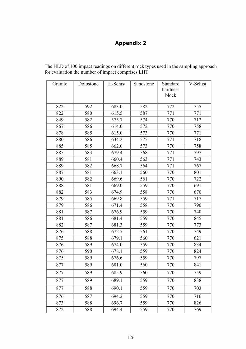
126
Appendix 2
The HLD of 100 impact readings on different rock types used in the sampling approach
for evaluation the number of impact comprises LHT
Granite Dolostone H-Schist Sandstone Standard
hardness
block
V-Schist
822 592 683.0 582 772 755
822 580 615.5 587 771 771
849 582 575.7 574 770 712
867 586 614.0 572 770 758
878 585 615.0 573 770 771
880 586 634.2 575 771 718
885 585 662.0 573 770 758
885 583 679.4 568 771 797
889 581 660.4 563 771 743
889 582 668.7 564 771 767
887 581 663.1 560 770 801
890 582 669.6 561 770 722
888 581 669.0 559 770 691
882 583 674.9 558 770 670
879 585 669.8 559 771 717
879 586 671.4 558 770 790
881 587 676.9 559 770 740
881 586 681.4 559 770 845
882 587 681.3 559 770 773
876 588 672.7 561 770 749
875 588 679.1 560 770 621
876 589 674.0 559 770 834
876 590 678.1 559 770 824
875 589 676.6 559 770 797
877 589 681.0 560 770 841
877 589 685.9 560 770 759
877 589 689.1 559 770 838
877 588 690.1 559 770 703
876 587 694.2 559 770 716
873 588 696.7 559 770 826
872 588 694.4 559 770 769

127
Granite Dolostone H-Schist Sandstone Standard
hardness
block
V-Schist
870 588 693.4 559 770 770
871 589 689.8 558 770 778
869 589 692.7 558 770 775
870 590 694.9 558 770 754
869 590 692.1 557 770 800
870 590 694.5 557 770 731
870 590 695.1 557 770 766
871 590 694.8 556 770 867
872 590 692.5 555 770 852
870 590 690.5 555 770 704
872 590 693.0 555 770 768
869 590 694.4 555 770 791
870 590 695.8 554 770 732
871 591 698.7 555 770 738
871 590 701.0 554 770 721
872 590 702.7 555 770 797
872 590 704.3 555 770 741
872 591 706.1 555 770 745
870 590 706.1 554 770 805
870 590 707.5 554 770 808
870 590 708.1 554 770 754
871 590 709.1 554 770 761
870 590 710.2 555 770 713
871 591 709.2 555 770 773
871 591 711.0 554 770 584
871 592 711.7 555 770 671
870 591 710.6 554 770 718
870 592 711.6 555 770 770
868 592 712.9 555 770 783
868 593 710.6 555 770 793
866 593 711.9 555 770 756
867 593 713.4 554 770 729
867 593 714.2 554 770 641
867 593 714.6 554 770 669
868 593 716.5 554 770 828
868 593 716.9 554 770 790
869 593 718.5 554 770 748
870 593 717.0 554 770 738
870 593 716.2 555 770 679
871 593 715.5 555 770 650

128
Granite Dolostone H-Schist Sandstone Standard
hardness
block
V-Schist
871 593 716.8 555 770 830
870 593 718.5 554 770 797
869 593 716.9 554 770 723
870 593 716.1 554 770 824
870 593 715.8 555 770 757
870 593 716.7 555 770 849
871 593 716.2 555 770 716
871 593 714.0 555 770 779
871 593 714.9 555 770 759
871 593 715.8 555 770 755
871 593 714.0 555 770 753
871 593 714.7 555 770 778
871 594 713.3 555 770 790
871 593 713.6 555 770 819
871 593 710.5 554 770 749
871 594 708.6 554 770 750
871 593 708.9 554 770 840
871 594 708.9 554 770 810
871 593 707.5 554 770 612
870 594 708.4 554 770 766
870 594 708.9 554 770 798
871 594 709.7 553 770 705
871 594 710.6 553 770 607
871 594 710.3 553 770 786
871 594 708.3 553 770 763
871 594 709.2 553 770 824
872 594 709.8 553 770 850
872 594 709.2 553 770 766
871 594 709.7 552 770 798

129
Comments on some UCS test specimens that were tested in this study.
ID Comments
SH4 Horizontal vein near top of sample.
SH5 Schistosity at top of sample, with approximately horizontal veins in the
center.
SH6 Slight angled veins at top and bottom.
SH7 No dominant mode.
SH8 Small slightly angled veins in center, traces of pyrite on ends of sample.
SH1
2
Sample failed immediately upon pre-loading. No acquired
SV6 It has fractures/ a crack along its side
C1 Holds concretion and microdefect laminated mud& silt sandstone with
ripple mark.
C3 Holds concretion and microdefect laminated mud& silt sandstone with
ripple mark.
C4 Holds concretion and microdefect laminated mud& silt sandstone with
ripple mark.
Description of Schist specimens after preparing
ID Schistosity Damage
SH 4 Nice horizontal veins at top. Small
inclusions elsewhere, no clear pattern.
Perfect top, small chips from saw
on bottom edge with a small dip
on the bottom surface. SH 5 Slight angled in middle, smaller vein
at top of sample.
Perfect top, small chips from saw
on bottom edge.
SH 6 Very little, small inclusions, slight
angled vein near bottom.
Small saw marks on top and
bottom edges.
SH 7 Two veins create eye shaped
patterning center.
Both ends in excellent shape.
SH 8 Horizontal vein on top, no other
significant pattern.
Tiny dip on top surface, with few
shallow saw marks on bottom
edge.
SH 9 Few inclusions, no pattern. No damage.
SH 10 Blotch of pyrite in center, several
veins dispersing on an angle from
center.
Small saw teeth marks on top
edge.
SH 11 Nice horizontal vein at the top, small
striations along column.
No damage.
SH 12 Three small, horizontal striations. No damage.
SV 2 Vertical grain, but no visible pyrite
inclusions.
Small chips along top and
bottom edge.
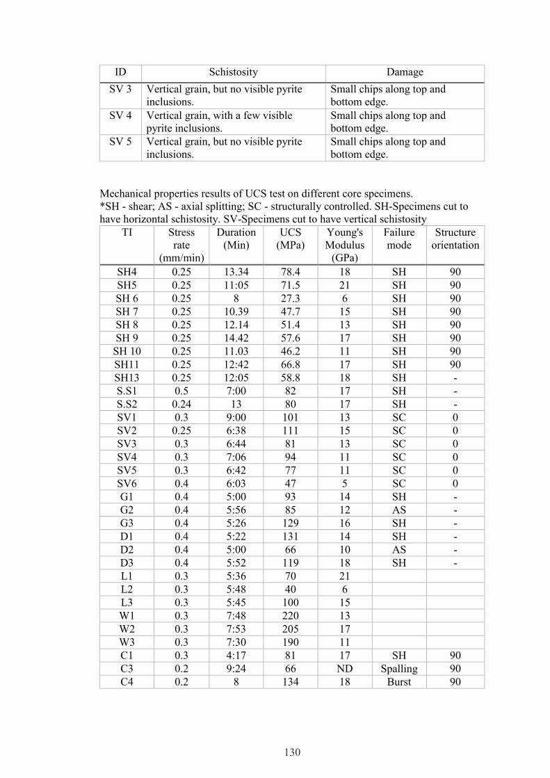
130
ID Schistosity Damage
SV 3 Vertical grain, but no visible pyrite
inclusions.
Small chips along top and
bottom edge.
SV 4 Vertical grain, with a few visible
pyrite inclusions.
Small chips along top and
bottom edge.
SV 5 Vertical grain, but no visible pyrite
inclusions.
Small chips along top and
bottom edge.
Mechanical properties results of UCS test on different core specimens.
*SH - shear; AS - axial splitting; SC - structurally controlled. SH-Specimens cut to
have horizontal schistosity. SV-Specimens cut to have vertical schistosity
TI Stress
rate
(mm/min)
Duration
(Min)
UCS
(MPa)
Young's
Modulus
(GPa)
Failure
mode
Structure
orientation
SH4 0.25 13.34 78.4 18 SH 90
SH5 0.25 11:05 71.5 21 SH 90
SH 6 0.25 8 27.3 6 SH 90
SH 7 0.25 10.39 47.7 15 SH 90
SH 8 0.25 12.14 51.4 13 SH 90
SH 9 0.25 14.42 57.6 17 SH 90
SH 10 0.25 11.03 46.2 11 SH 90
SH11 0.25 12:42 66.8 17 SH 90
SH13 0.25 12:05 58.8 18 SH -
S.S1 0.5 7:00 82 17 SH -
S.S2 0.24 13 80 17 SH -
SV1 0.3 9:00 101 13 SC 0
SV2 0.25 6:38 111 15 SC 0
SV3 0.3 6:44 81 13 SC 0
SV4 0.3 7:06 94 11 SC 0
SV5 0.3 6:42 77 11 SC 0
SV6 0.4 6:03 47 5 SC 0
G1 0.4 5:00 93 14 SH -
G2 0.4 5:56 85 12 AS -
G3 0.4 5:26 129 16 SH -
D1 0.4 5:22 131 14 SH -
D2 0.4 5:00 66 10 AS -
D3 0.4 5:52 119 18 SH -
L1 0.3 5:36 70 21
L2 0.3 5:48 40 6
L3 0.3 5:45 100 15
W1 0.3 7:48 220 13
W2 0.3 7:53 205 17
W3 0.3 7:30 190 11
C1 0.3 4:17 81 17 SH 90
C3 0.2 9:24 66 ND Spalling 90
C4 0.2 8 134 18 Burst 90
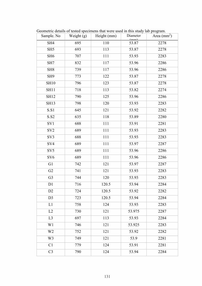
131
Geometric details of tested specimens that were used in this study lab program.
Sample. No Weight (g) Height (mm) Diameter
(mm) Area (mm2)
SH4 695 110 53.87 2278
SH5 693 113 53.87 2278
SH6 707 111 53.93 2283
SH7 832 117 53.96 2286
SH8 739 117 53.96 2286
SH9 773 122 53.87 2278
SH10 796 123 53.87 2278
SH11 718 113 53.82 2274
SH12 790 125 53.96 2286
SH13 798 120 53.93 2283
S.S1 645 121 53.92 2282
S.S2 635 118
53.89 2280
SV1 688 111 53.91 2281
SV2 689 111 53.93 2283
SV3 688 111 53.93 2283
SV4 689 111 53.97 2287
SV5 689 111 53.96 2286
SV6 689 111 53.96 2286
G1 742 121 53.97 2287
G2 741 121 53.93 2283
G3 744 120 53.93 2283
D1 716 120.5 53.94 2284
D2 724 120.5 53.92 2282
D3 723 120.5 53.94 2284
L1 758 124 53.93 2283
L2 730 121 53.975 2287
L3 697 113 53.93 2284
W1 746 121 53.925 2283
W2 752 121 53.92 2282
W3 749 121 53.9 2281
C1 779 124 53.91 2281
C3 790 124 53.94 2284

132
Sample. No Weight (g) Height (mm) Diameter
(mm) Area (mm2)
C4 798 124 53.93 2283
Selected sample presented in the sandstone conference paper.
HL
D
Actual
UCS
(MPa)
Nonlinea
r UCS
(MPa)
(MPa)
95% CI
Least
squar
e
UCS
(MPa)
95%
CI
Grain size Source
631 91.7 75.75 ±
11
72.70
± 8 Fine
Meulenkamp & Grima,
1999
714 91.7 118.20
± 10
111.7
± 13
Fine, slightly
weathered Asef, M, 1995
620 82 71.328
±11
68.59
± 7 Fine Verwaal & Mulder, 1993
606 77 66.124
±11
63.76
± 7 Fine Verwaal & Mulder, 1993
659 36.8 87.814
±10
83.83
± 9 Fine Asef, M, 1995
677 35.4 96.627
±10
91.93
± 10 Fine Asef, M, 1995
412 31 23.354
±8.
23.36
± 5 Fine Verwaal & Mulder, 1993
315 15 13.883
±6
14.14
± 4 Calcareous Verwaal & Mulder, 1993
595 38 62.329
±11
60.22
± 7
Conglomerat
e
Meulenkamp & Grima,
1999
591 35.4 61.102
±11
59.08
± 7
Conglomerat
e
Meulenkamp & Grima,
1999
809 219.651 196.914
±19
182.7
3 ± 31 Greywacke Present study
787 204.575 175.338
±15
163.3
7 ± 25 Greywacke Present study
833 189.889 223.535
±26
206.5
1 ± 38 Greywacke Present study
770 198 159.346
±13
148.9
7 ± 21
Massive
Micaceous Verwaal and Mulder, 1993
788 142 175.809
±16
163.7
9 ± 25
Micaceous,
medium
grained
Verwaal & Mulder, 1993
667 75.9 91.966
±10
87.65
± 9.2 Medium
Meulenkamp & Grima,
1999
649 72.7 83.265
±11
79.64
± 8.3 Medium
Meulenkamp & Grima,
1999
627 59.4 73.863
±11
70.94
± 7 Medium Asef, M, 1995
576 52.3 56.31
±11
54.60
± 7 Medium
Meulenkamp & Grima,
1999
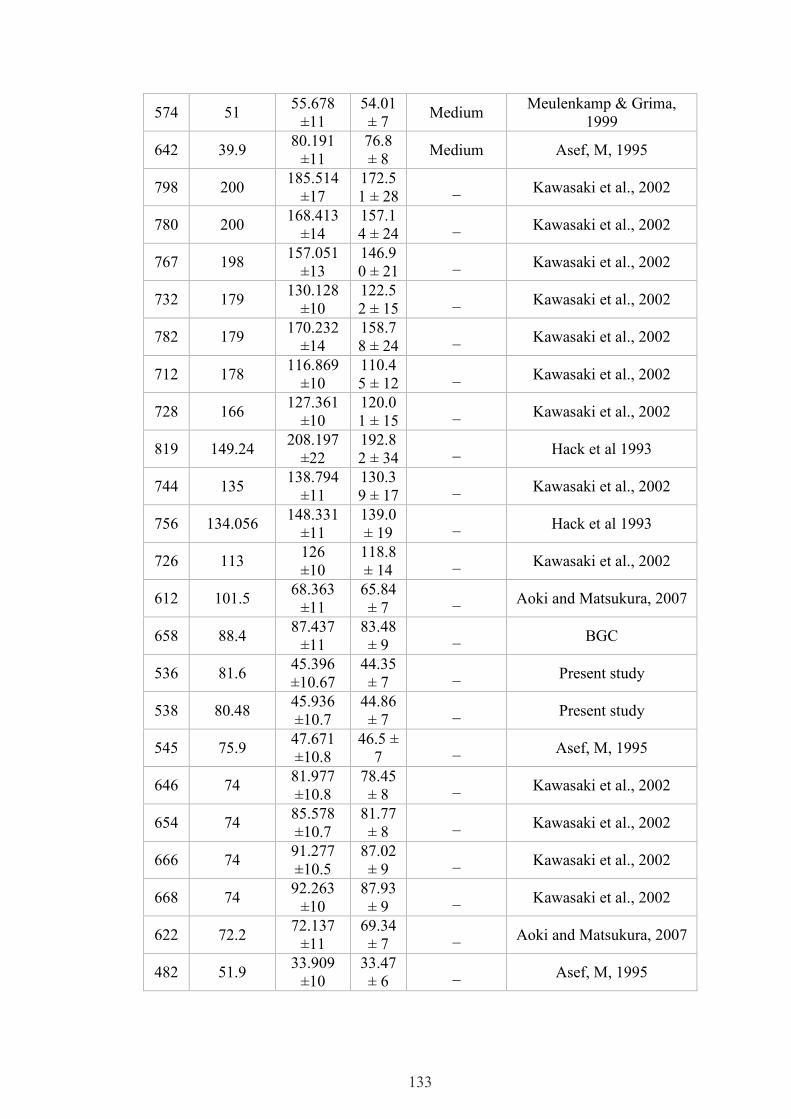
133
574 51 55.678
±11
54.01
± 7 Medium
Meulenkamp & Grima,
1999
642 39.9 80.191
±11
76.8
± 8 Medium Asef, M, 1995
798 200 185.514
±17
172.5
1 ± 28 _ Kawasaki et al., 2002
780 200 168.413
±14
157.1
4 ± 24 _ Kawasaki et al., 2002
767 198 157.051
±13
146.9
0 ± 21 _ Kawasaki et al., 2002
732 179 130.128
±10
122.5
2 ± 15 _ Kawasaki et al., 2002
782 179 170.232
±14
158.7
8 ± 24 _ Kawasaki et al., 2002
712 178 116.869
±10
110.4
5 ± 12 _ Kawasaki et al., 2002
728 166 127.361
±10
120.0
1 ± 15 _ Kawasaki et al., 2002
819 149.24 208.197
±22
192.8
2 ± 34 _ Hack et al 1993
744 135 138.794
±11
130.3
9 ± 17 _ Kawasaki et al., 2002
756 134.056 148.331
±11
139.0
± 19 _ Hack et al 1993
726 113 126
±10
118.8
± 14 _ Kawasaki et al., 2002
612 101.5 68.363
±11
65.84
± 7 _ Aoki and Matsukura, 2007
658 88.4 87.437
±11
83.48
± 9 _ BGC
536 81.6 45.396
±10.67
44.35
± 7 _ Present study
538 80.48 45.936
±10.7
44.86
± 7 _ Present study
545 75.9 47.671
±10.8
46.5 ±
7 _ Asef, M, 1995
646 74 81.977
±10.8
78.45
± 8 _ Kawasaki et al., 2002
654 74 85.578
±10.7
81.77
± 8 _ Kawasaki et al., 2002
666 74 91.277
±10.5
87.02
± 9 _ Kawasaki et al., 2002
668 74 92.263
±10
87.93
± 9 _ Kawasaki et al., 2002
622 72.2 72.137
±11
69.34
± 7 _ Aoki and Matsukura, 2007
482 51.9 33.909
±10
33.47
± 6 _ Asef, M, 1995

134
591 37 60.905
±11
58.90
± 7 _ Asef, M, 1995
450 14.5 28.522
±9
28.33
± 6
Red,
weathered,
porous.
Asef, M, 1995

135
Geometric description of UCS tested Schist used in presented lab program
Sample
#
Hole # Depth
(m)
Length
. avg
Dia.
avg
L/
D
Area
(mm2)
Weight
(g)
Volume
(cm3)
1 RMUG14-
252,Box-8
42.96-
43.17
80.54 36.
18
2.2
3
1027.37 243.33 82.74
2 RMUG14-
252,Box-8
47.86-
48.14
79.81 36.
11
2.2
1
1023.59 230.82 81.70
1 RMUG14-
252,Box-15
85.56-
85.75
80.36 36.
14
2.2
2
1025.48 233.19 82.41
1 RMUG14-
249,Box-3
14.37-
14.64
79.83 36.
18
2.2
1
1027.56 232.16 82.03
2 RMUG14-
249,Box-14
76.58-
76.83
80.26 36.
20
2.2
2
1028.88 229.18 82.57
3 RMUG14-
249,Box-19
103.6-
103.89
78.96 36.
18
2.1
8
1027.75 224.11 81.15
4 RMUG14-
249,Box-19
104.46-
104.72
80.03 36.
19
2.2
1
1027.94 227.98 82.27
5 RMUG14-
249,Box-22
120.25-
120.52
80.19 36.
19
2.2
2
1027.94 251.56 82.43
6 RMUG14-
249,Box-22
121.68-
121.9
80.39 36.
17
2.2
2
1026.80 240.73 82.55
7 RMUG14-
249,Box-23
128.0-
128.25
80.37 36.
15
2.2
2
1025.86 271.01 82.45
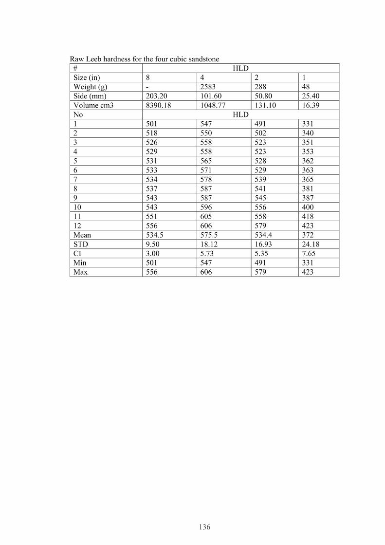
136
Raw Leeb hardness for the four cubic sandstone
# HLD
Size (in) 8 4 2 1
Weight (g) - 2583 288 48
Side (mm) 203.20 101.60 50.80 25.40
Volume cm3 8390.18 1048.77 131.10 16.39
No HLD
1 501 547 491 331
2 518 550 502 340
3 526 558 523 351
4 529 558 523 353
5 531 565 528 362
6 533 571 529 363
7 534 578 539 365
8 537 587 541 381
9 543 587 545 387
10 543 596 556 400
11 551 605 558 418
12 556 606 579 423
Mean 534.5 575.5 534.4 372
STD 9.50 18.12 16.93 24.18
CI 3.00 5.73 5.35 7.65
Min 501 547 491 331
Max 556 606 579 423

137
Figure 4.11 Stress - Strain curves of schist specimens, using strain gauge and Linear
Variable Differential Transformer (LVDT), which are
transducers to measure the displacement for schist core specimens
under UCS tests.
0
10
20
30
40
50
60
70
-0.5 0 0.5 1
RMUG14-249,Box-3,sample#1
axial1
axial2
lateral1
Lateral2
LVDT
0
5000
10000
15000
20000
25000
30000
35000
40000
45000
-0.5 0 0.5 1
RMUG14-249,Box-14,sample#2
axial1
axial2
lateral1
lateral2
LVDT
-5000
0
5000
10000
15000
20000
25000
30000
-0.5 0 0.5 1
RMUG14-249,Box-19,sample#4
axial1
axial2
lateral1
lateral2
LVDT
0
10000
20000
30000
40000
50000
60000
70000
80000
-2 -1.5 -1 -0.5 0 0.5 1
RMUG14-249,Box-22,sample5
axial1
axial2
lateral1
lateral2
LVDT
0
5000
10000
15000
20000
25000
30000
-0.5 0 0.5 1
RMUG14-249,Box-22sample6
axial1
axial2
lateral1
lateral2
Series5
0
10000
20000
30000
40000
50000
60000
-0.5 0 0.5 1
RMUG14-249,Box-23sample7
axial1
axial2
lateral1
lateral2
LVDT
0
5000
10000
15000
20000
25000
30000
35000
40000
45000
50000
-0.5 0 0.5 1
RMUG14-252,Box-8sample1
axial2
axial1
lateral2
lateral1
LVDT
0
5000
10000
15000
20000
25000
30000
-0.5 0 0.5 1
RMUG14-249,Box-19,sample#3
axial1
axial2
lateral1
LVDT
lateral2
0
2000
4000
6000
8000
10000
12000
14000
16000
18000
20000
-0.5 0 0.5 1
RMUG14-252,Box-15,sample#1
axial1
axial2
lateral1
lateral2
LVDT
0
5000
10000
15000
20000
25000
30000
-0.5 0 0.5 1
RMUG14-252,Box-8sample2
LVDT
axial2
axial1
lateral1
lateral2
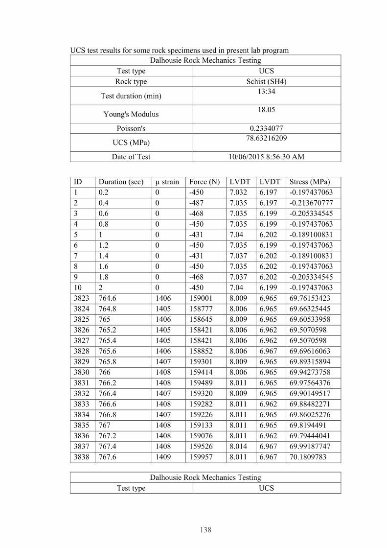
138
UCS test results for some rock specimens used in present lab program
Dalhousie Rock Mechanics Testing
Test type UCS
Rock type Schist (SH4)
Test duration (min) 13:34
Young's Modulus 18.05
Poisson's 0.2334077
UCS (MPa) 78.63216209
Date of Test 10/06/2015 8:56:30 AM
ID Duration (sec) µ strain Force (N) LVDT LVDT Stress (MPa)
1 0.2 0 -450 7.032 6.197 -0.197437063
2 0.4 0 -487 7.035 6.197 -0.213670777
3 0.6 0 -468 7.035 6.199 -0.205334545
4 0.8 0 -450 7.035 6.199 -0.197437063
5 1 0 -431 7.04 6.202 -0.189100831
6 1.2 0 -450 7.035 6.199 -0.197437063
7 1.4 0 -431 7.037 6.202 -0.189100831
8 1.6 0 -450 7.035 6.202 -0.197437063
9 1.8 0 -468 7.037 6.202 -0.205334545
10 2 0 -450 7.04 6.199 -0.197437063
3823 764.6 1406 159001 8.009 6.965 69.76153423
3824 764.8 1405 158777 8.006 6.965 69.66325445
3825 765 1406 158645 8.009 6.965 69.60533958
3826 765.2 1405 158421 8.006 6.962 69.5070598
3827 765.4 1405 158421 8.006 6.962 69.5070598
3828 765.6 1406 158852 8.006 6.967 69.69616063
3829 765.8 1407 159301 8.009 6.965 69.89315894
3830 766 1408 159414 8.006 6.965 69.94273758
3831 766.2 1408 159489 8.011 6.965 69.97564376
3832 766.4 1407 159320 8.009 6.965 69.90149517
3833 766.6 1408 159282 8.011 6.962 69.88482271
3834 766.8 1407 159226 8.011 6.965 69.86025276
3835 767 1408 159133 8.011 6.965 69.8194491
3836 767.2 1408 159076 8.011 6.962 69.79444041
3837 767.4 1408 159526 8.014 6.967 69.99187747
3838 767.6 1409 159957 8.011 6.967 70.1809783
Dalhousie Rock Mechanics Testing
Test type UCS

139
Rock type G1
Test duration (min) 5.5
Young's Modulus 13.576
Poisson's -
UCS (MPa) 93
Date of Test Wed 09 Feb 2005 00:25:12
Time (min) Position (mm) Strain Load (N) Stress (MPa)
0 0 0 0 0
0.00167 0 0 -6 -0.0026309
0.00333 0 0 -7 -0.0030694
0.005 0 0 -6 -0.0026309
0.00667 0 0 -6 -0.0026309
0.00833 0 0 -7 -0.0030694
0.01 0 0 -5 -0.0021924
0.01167 0 0 -2 -0.000877
0.01333 0 0 0 0
0.015 0 0 0 0
0.01667 0.0063 5.2234E-05 5 0.00219242
0.01833 0.0063 5.2234E-05 3 0.00131545
0.02 0.0063 5.2234E-05 2 0.00087697
0.02167 0.0063 5.2234E-05 2 0.00087697
0.02333 0.0063 5.2234E-05 -5 -0.0021924
0.025 0.0063 5.2234E-05 -9 -0.0039463
0.02667 0.0063 5.2234E-05 -7 -0.0030694
0.02833 0.0063 5.2234E-05 -8 -0.0035079
0.03 0.0063 5.2234E-05 -3 -0.0013154
0.03167 0.0063 5.2234E-05 -2 -0.000877
0.03333 0.0063 5.2234E-05 -2 -0.000877
0.035 0.0127 0.0001053 3 0.00131545
0.03667 0.0127 0.0001053 8 0.00350786
0.03833 0.0127 0.0001053 9 0.00394635
0.04 0.0127 0.0001053 5 0.00219242
0.04167 0.0127 0.0001053 5 0.00219242
0.04333 0.0127 0.0001053 6 0.0026309
0.045 0.0127 0.0001053 5 0.00219242
0.04667 0.0127 0.0001053 6 0.0026309
0.04833 0.0127 0.0001053 15 0.00657725
0.05 0.019 0.00015753 21 0.00920814
0.05167 0.019 0.00015753 21 0.00920814
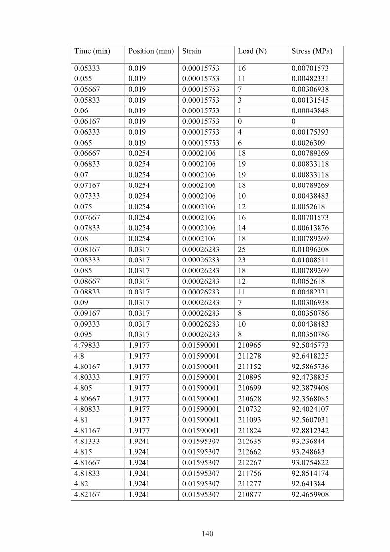
140
Time (min) Position (mm) Strain Load (N) Stress (MPa)
0.05333 0.019 0.00015753 16 0.00701573
0.055 0.019 0.00015753 11 0.00482331
0.05667 0.019 0.00015753 7 0.00306938
0.05833 0.019 0.00015753 3 0.00131545
0.06 0.019 0.00015753 1 0.00043848
0.06167 0.019 0.00015753 0 0
0.06333 0.019 0.00015753 4 0.00175393
0.065 0.019 0.00015753 6 0.0026309
0.06667 0.0254 0.0002106 18 0.00789269
0.06833 0.0254 0.0002106 19 0.00833118
0.07 0.0254 0.0002106 19 0.00833118
0.07167 0.0254 0.0002106 18 0.00789269
0.07333 0.0254 0.0002106 10 0.00438483
0.075 0.0254 0.0002106 12 0.0052618
0.07667 0.0254 0.0002106 16 0.00701573
0.07833 0.0254 0.0002106 14 0.00613876
0.08 0.0254 0.0002106 18 0.00789269
0.08167 0.0317 0.00026283 25 0.01096208
0.08333 0.0317 0.00026283 23 0.01008511
0.085 0.0317 0.00026283 18 0.00789269
0.08667 0.0317 0.00026283 12 0.0052618
0.08833 0.0317 0.00026283 11 0.00482331
0.09 0.0317 0.00026283 7 0.00306938
0.09167 0.0317 0.00026283 8 0.00350786
0.09333 0.0317 0.00026283 10 0.00438483
0.095 0.0317 0.00026283 8 0.00350786
4.79833 1.9177 0.01590001 210965 92.5045773
4.8 1.9177 0.01590001 211278 92.6418225
4.80167 1.9177 0.01590001 211152 92.5865736
4.80333 1.9177 0.01590001 210895 92.4738835
4.805 1.9177 0.01590001 210699 92.3879408
4.80667 1.9177 0.01590001 210628 92.3568085
4.80833 1.9177 0.01590001 210732 92.4024107
4.81 1.9177 0.01590001 211093 92.5607031
4.81167 1.9177 0.01590001 211824 92.8812342
4.81333 1.9241 0.01595307 212635 93.236844
4.815 1.9241 0.01595307 212662 93.248683
4.81667 1.9241 0.01595307 212267 93.0754822
4.81833 1.9241 0.01595307 211756 92.8514174
4.82 1.9241 0.01595307 211277 92.641384
4.82167 1.9241 0.01595307 210877 92.4659908
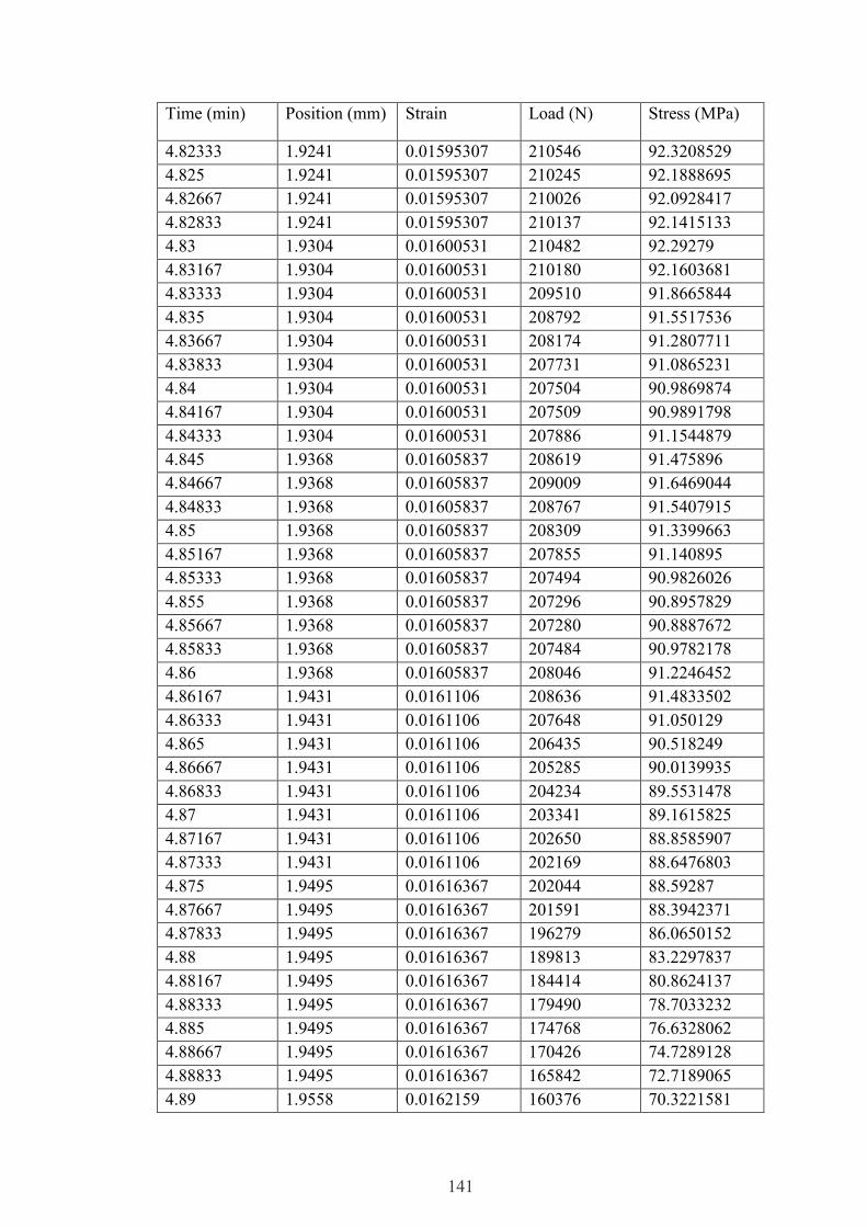
141
Time (min) Position (mm) Strain Load (N) Stress (MPa)
4.82333 1.9241 0.01595307 210546 92.3208529
4.825 1.9241 0.01595307 210245 92.1888695
4.82667 1.9241 0.01595307 210026 92.0928417
4.82833 1.9241 0.01595307 210137 92.1415133
4.83 1.9304 0.01600531 210482 92.29279
4.83167 1.9304 0.01600531 210180 92.1603681
4.83333 1.9304 0.01600531 209510 91.8665844
4.835 1.9304 0.01600531 208792 91.5517536
4.83667 1.9304 0.01600531 208174 91.2807711
4.83833 1.9304 0.01600531 207731 91.0865231
4.84 1.9304 0.01600531 207504 90.9869874
4.84167 1.9304 0.01600531 207509 90.9891798
4.84333 1.9304 0.01600531 207886 91.1544879
4.845 1.9368 0.01605837 208619 91.475896
4.84667 1.9368 0.01605837 209009 91.6469044
4.84833 1.9368 0.01605837 208767 91.5407915
4.85 1.9368 0.01605837 208309 91.3399663
4.85167 1.9368 0.01605837 207855 91.140895
4.85333 1.9368 0.01605837 207494 90.9826026
4.855 1.9368 0.01605837 207296 90.8957829
4.85667 1.9368 0.01605837 207280 90.8887672
4.85833 1.9368 0.01605837 207484 90.9782178
4.86 1.9368 0.01605837 208046 91.2246452
4.86167 1.9431 0.0161106 208636 91.4833502
4.86333 1.9431 0.0161106 207648 91.050129
4.865 1.9431 0.0161106 206435 90.518249
4.86667 1.9431 0.0161106 205285 90.0139935
4.86833 1.9431 0.0161106 204234 89.5531478
4.87 1.9431 0.0161106 203341 89.1615825
4.87167 1.9431 0.0161106 202650 88.8585907
4.87333 1.9431 0.0161106 202169 88.6476803
4.875 1.9495 0.01616367 202044 88.59287
4.87667 1.9495 0.01616367 201591 88.3942371
4.87833 1.9495 0.01616367 196279 86.0650152
4.88 1.9495 0.01616367 189813 83.2297837
4.88167 1.9495 0.01616367 184414 80.8624137
4.88333 1.9495 0.01616367 179490 78.7033232
4.885 1.9495 0.01616367 174768 76.6328062
4.88667 1.9495 0.01616367 170426 74.7289128
4.88833 1.9495 0.01616367 165842 72.7189065
4.89 1.9558 0.0162159 160376 70.3221581
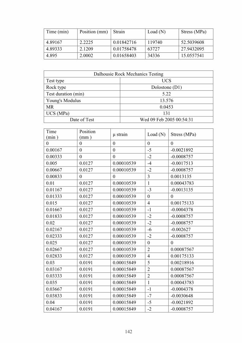
142
Time (min) Position (mm) Strain Load (N) Stress (MPa)
4.89167 2.2225 0.01842716 119740 52.5039608
4.89333 2.1209 0.01758478 63727 27.9432095
4.895 2.0002 0.01658403 34336 15.0557541
Dalhousie Rock Mechanics Testing
Test type UCS
Rock type Dolostone (D1)
Test duration (min) 5.22
Young's Modulus 13.576
MR 0.0453
UCS (MPa) 131
Date of Test Wed 09 Feb 2005 00:54:31
Time
(min )
Position
(mm ) μ strain Load (N) Stress (MPa)
0 0 0 0 0
0.00167 0 0 -5 -0.0021892
0.00333 0 0 -2 -0.0008757
0.005 0.0127 0.00010539 -4 -0.0017513
0.00667 0.0127 0.00010539 -2 -0.0008757
0.00833 0 0 3 0.0013135
0.01 0.0127 0.00010539 1 0.00043783
0.01167 0.0127 0.00010539 -3 -0.0013135
0.01333 0.0127 0.00010539 0 0
0.015 0.0127 0.00010539 4 0.00175133
0.01667 0.0127 0.00010539 -1 -0.0004378
0.01833 0.0127 0.00010539 -2 -0.0008757
0.02 0.0127 0.00010539 -2 -0.0008757
0.02167 0.0127 0.00010539 -6 -0.002627
0.02333 0.0127 0.00010539 -2 -0.0008757
0.025 0.0127 0.00010539 0 0
0.02667 0.0127 0.00010539 2 0.00087567
0.02833 0.0127 0.00010539 4 0.00175133
0.03 0.0191 0.00015849 5 0.00218916
0.03167 0.0191 0.00015849 2 0.00087567
0.03333 0.0191 0.00015849 2 0.00087567
0.035 0.0191 0.00015849 1 0.00043783
0.03667 0.0191 0.00015849 -1 -0.0004378
0.03833 0.0191 0.00015849 -7 -0.0030648
0.04 0.0191 0.00015849 -5 -0.0021892
0.04167 0.0191 0.00015849 -2 -0.0008757

143
Time
(min )
Position
(mm ) μ strain Load (N) Stress (MPa)
0.04333 0.0191 0.00015849 -4 -0.0017513
0.045 0.0191 0.00015849 -2 -0.0008757
0.04667 0.0191 0.00015849 -2 -0.0008757
0.04833 0.0254 0.00021077 7 0.00306483
0.05 0.0254 0.00021077 9 0.0039405
5.32667 2.1336 0.01770475 296355 129.753989
5.32833 2.1336 0.01770475 296037 129.614758
5.33 2.1336 0.01770475 295883 129.547332
5.33167 2.1336 0.01770475 296000 129.598558
5.33333 2.1336 0.01770475 296471 129.804778
5.335 2.1336 0.01770475 297253 130.147163
5.33667 2.1399 0.01775703 298288 130.60032
5.33833 2.1399 0.01775703 298770 130.811356
5.34 2.1399 0.01775703 298649 130.758378
5.34167 2.1399 0.01775703 298333 130.620023
5.34333 2.1399 0.01775703 298019 130.482543
5.345 2.1399 0.01775703 297813 130.392349
5.34667 2.1399 0.01775703 297778 130.377025
5.34833 2.1399 0.01775703 298033 130.488673
5.35 2.1463 0.01781014 298607 130.739989
5.35167 2.1463 0.01781014 299048 130.933073
5.35333 2.1463 0.01781014 298700 130.780707
5.355 2.1463 0.01781014 297996 130.472473
5.35667 2.1463 0.01781014 297287 130.162049
5.35833 2.1463 0.01781014 296750 129.926933
5.36 2.1463 0.01781014 296204 129.687876
5.36167 2.1463 0.01781014 294889 129.112126
5.36333 2.1463 0.01781014 293394 128.457566
5.365 2.1527 0.01786325 292045 127.866929
5.36667 2.2035 0.01828479 290035 126.986885
5.36833 2.4447 0.02028628 180012 78.8151881
5.37 2.3876 0.01981246 96516 42.2578866
5.37167 2.2352 0.01854784 51871 22.7108338

144
Details of database that were used in this study
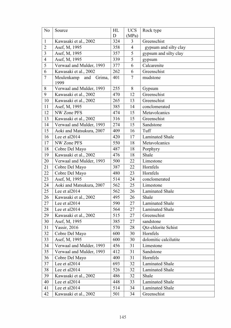
145
No Source HL
D
UCS
(MPa)
Rock type
1 Kawasaki et al., 2002 324 3 Greenschist
2 Asef, M, 1995 358 4 gypsum and silty clay
3 Asef, M, 1995 357 5 gypsum and silty clay
4 Asef, M, 1995 339 5 gypsum
5 Verwaal and Mulder, 1993 377 6 Calcarenite
6 Kawasaki et al., 2002 262 6 Greenschist
7 Meulenkamp and Grima,
1999
401 7 mudstone
8 Verwaal and Mulder, 1993 255 8 Gypsum
9 Kawasaki et al., 2002 470 12 Greenschist
10 Kawasaki et al., 2002 265 13 Greenschist
11 Asef, M, 1995 385 14 conclomerated
12 NW Zone PFS 474 15 Metavolcanics
13 Kawasaki et al., 2002 316 15 Greenschist
14 Verwaal and Mulder, 1993 274 15 Sandstone
15 Aoki and Matsukura, 2007 409 16 Tuff
16 Lee et al2014 420 17 Laminated Shale
17 NW Zone PFS 550 18 Metavolcanics
18 Cobre Del Mayo 487 18 Porphyry
19 Kawasaki et al., 2002 476 18 Shale
20 Verwaal and Mulder, 1993 500 22 Limestone
21 Cobre Del Mayo 387 22 Hornfels
22 Cobre Del Mayo 480 23 Hornfels
23 Asef, M, 1995 514 24 conclomerated
24 Aoki and Matsukura, 2007 562 25 Limestone
25 Lee et al2014 562 26 Laminated Shale
26 Kawasaki et al., 2002 495 26 Shale
27 Lee et al2014 590 27 Laminated Shale
28 Lee et al2014 564 27 Laminated Shale
29 Kawasaki et al., 2002 515 27 Greenschist
30 Asef, M, 1995 385 27 sandstone
31 Yassir, 2016 570 28 Qtz-chlorite Schist
32 Cobre Del Mayo 600 30 Hornfels
33 Asef, M, 1995 600 30 dolomitic calcilutite
34 Verwaal and Mulder, 1993 456 31 Limestone
35 Verwaal and Mulder, 1993 412 31 Sandstone
36 Cobre Del Mayo 400 31 Hornfels
37 Lee et al2014 693 32 Laminated Shale
38 Lee et al2014 526 32 Laminated Shale
39 Kawasaki et al., 2002 486 32 Shale
40 Lee et al2014 448 33 Laminated Shale
41 Lee et al2014 514 34 Laminated Shale
42 Kawasaki et al., 2002 501 34 Greenschist

146
43 Lee et al2014 591 35 Laminated Shale
44 Coal Valley 537 35 Siltstone
45 Meulenkamp and Grima,
1999
455 35 sandstone
46 Lee et al2014 548 36 Laminated Shale
47 Lee et al2014 500 37 Laminated Shale
48 Lee et al2014 601 38 Laminated Shale
49 Meulenkamp and Grima,
1999
595 38 sandstone
50 Yassir, 2016 555 38 Mafic Dyke
51 Lee et al2014 464 38 Laminated Shale
52 Verwaal and Mulder, 1993 539 39 Dolomite
53 Verwaal and Mulder, 1993 526 39 Limestone
54 Yassir, 2016 574 40 limestone
55 Lee et al2014 504 41 Laminated Shale
56 Lee et al2014 439 42 Laminated Shale
57 Lee et al2014 447 43 Laminated Shale
58 Coal Valley 644 44 Siltstone
59 Lee et al2014 523 44 Laminated Shale
60 Asef, M, 1995 695 45 conglomerates
61 Kawasaki et al., 2002 583 45 Greenschist
62 Lee et al2014 662 46 Laminated Shale
63 Lee et al2014 526 46 Laminated Shale
64 yassir2016 466 46 schist-H
65 Lee et al2014 553 47 Laminated Shale
66 Lee et al2014 471 48 Laminated Shale
67 yassir2016 464 48 schist-H
68 Lee et al2014 536 50 Laminated Shale
69 Lee et al2014 670 51 Laminated Shale
70 Lee et al2014 574 51 Laminated Shale
71 Lee et al2014 547 51 Laminated Shale
72 Meulenkamp and Grima,
1999
531 51 sandstone
73 yassir2016 531 51 schist-H
74 Lee et al2014 502 51 Laminated Shale
75 Cobre Del Mayo 630 52 Porphyry
76 Meulenkamp and Grima,
1999
576 52 sandstone
77 Cobre Del Mayo 558 54 Porphyry
78 Lee et al2014 527 54 Laminated Shale
79 Lee et al2014 576 55 Laminated Shale
80 Lee et al2014 526 55 Laminated Shale
81 Lee et al2014 523 55 Laminated Shale
82 Lee et al2014 480 55 Laminated Shale
83 Lee et al2014 520 56 Laminated Shale
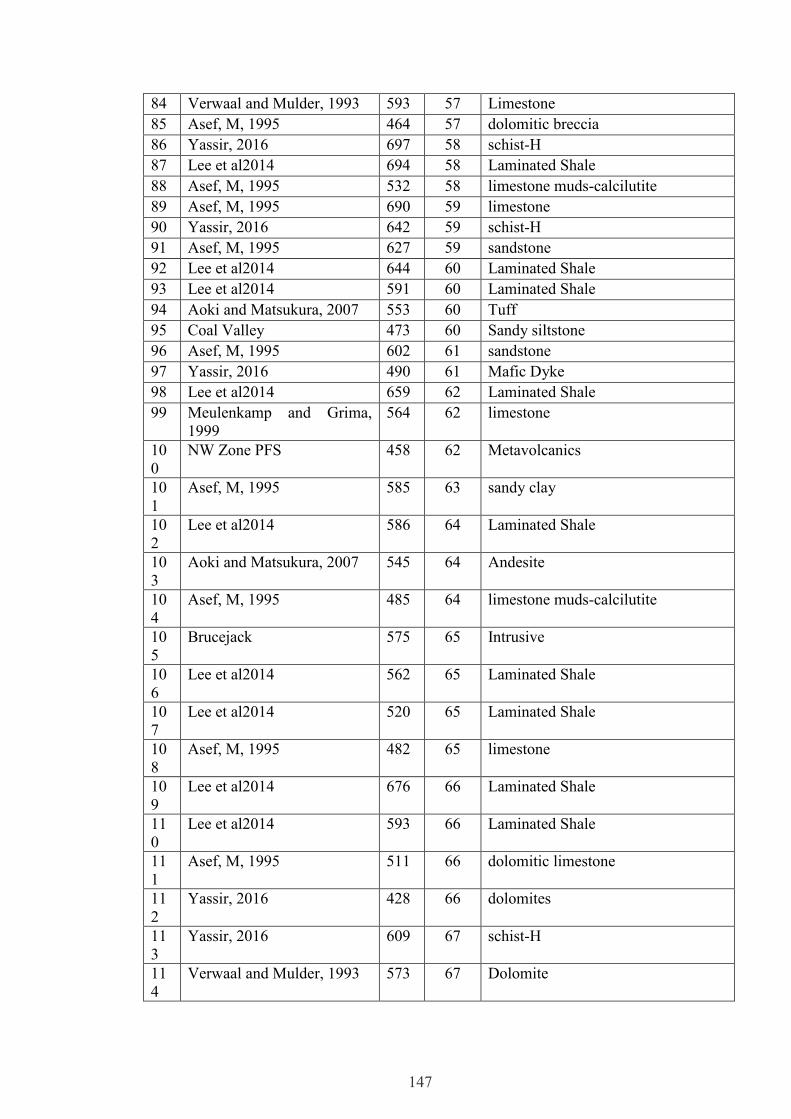
147
84 Verwaal and Mulder, 1993 593 57 Limestone
85 Asef, M, 1995 464 57 dolomitic breccia
86 Yassir, 2016 697 58 schist-H
87 Lee et al2014 694 58 Laminated Shale
88 Asef, M, 1995 532 58 limestone muds-calcilutite
89 Asef, M, 1995 690 59 limestone
90 Yassir, 2016 642 59 schist-H
91 Asef, M, 1995 627 59 sandstone
92 Lee et al2014 644 60 Laminated Shale
93 Lee et al2014 591 60 Laminated Shale
94 Aoki and Matsukura, 2007 553 60 Tuff
95 Coal Valley 473 60 Sandy siltstone
96 Asef, M, 1995 602 61 sandstone
97 Yassir, 2016 490 61 Mafic Dyke
98 Lee et al2014 659 62 Laminated Shale
99 Meulenkamp and Grima,
1999
564 62 limestone
10
0
NW Zone PFS 458 62 Metavolcanics
10
1
Asef, M, 1995 585 63 sandy clay
10
2
Lee et al2014 586 64 Laminated Shale
10
3
Aoki and Matsukura, 2007 545 64 Andesite
10
4
Asef, M, 1995 485 64 limestone muds-calcilutite
10
5
Brucejack 575 65 Intrusive
10
6
Lee et al2014 562 65 Laminated Shale
10
7
Lee et al2014 520 65 Laminated Shale
10
8
Asef, M, 1995 482 65 limestone
10
9
Lee et al2014 676 66 Laminated Shale
11
0
Lee et al2014 593 66 Laminated Shale
11
1
Asef, M, 1995 511 66 dolomitic limestone
11
2
Yassir, 2016 428 66 dolomites
11
3
Yassir, 2016 609 67 schist-H
11
4
Verwaal and Mulder, 1993 573 67 Dolomite

148
11
5
Lee et al2014 493 68 Laminated Shale
11
6
Yassir, 2016 689 69 Qtz-chlorite Schist
11
7
Lee et al2014 542 69 Laminated Shale
11
8
Yassir, 2016 655 70 limestone
11
9
Asef, M, 1995 620 71 calcilutite
12
0
Verwaal and Mulder, 1993 587 71 Limestone
12
1
Yassir, 2016 655 72 schist-H
12
2
Brucejack 622 72 Intrusive
12
3
Aoki and Matsukura, 2007 576 72 Sandstone
12
4
Lee et al2014 472 72 Laminated Shale
12
5
Meulenkamp and Grima,
1999
659 73 sandstone
12
6
Meulenkamp and Grima,
1999
649 73 limestone
12
7
Verwaal and Mulder, 1993 668 74 Limestone
12
8
Kawasaki et al., 2002 666 74 Sandstone
12
9
Kawasaki et al., 2002 654 74 Sandstone
13
0
Kawasaki et al., 2002 646 74 Sandstone
13
1
Kawasaki et al., 2002 627 74 Sandstone
13
2
RoxGold 646 75 Mafiv Volcanic
13
3
Lee et al2014 608 75 Laminated Shale
13
4
Meulenkamp and Grima,
1999
516 75 dolomite
13
5
Miller-Braeside 667 76 Limestone
13
6
Asef, M, 1995 621 76 sandstone
13
7
Meulenkamp and Grima,
1999
545 76 sandstone
13
8
Yassir, 2016 790 77 schist-V

149
13
9
Verwaal and Mulder, 1993 682 77 sandstone
14
0
Kawasaki et al., 2002 606 77 Shale
14
1
Lee et al2014 582 77 Laminated Shale
14
2
Lee et al2014 564 77 Laminated Shale
14
3
yassir2016 669 78 schist-H
14
4
Lee et al2014 564 78 Laminated Shale
14
5
Brucejack 642 80 Intrusive
14
6
Yassir, 2016 538 80 sandstone
14
7
Miller-Braeside 786 81 Limestone
14
8
Yassir, 2016 702 81 schist-V
14
9
Yassir, 2016 620 82 sandstone
15
0
Verwaal and Mulder, 1993 536 82 Sandstone
15
1
Verwaal and Mulder, 1993 783 85 Limestone
15
2
Yassir, 2016 637 85 granite
15
3
Meulenkamp and Grima,
1999
647 86 dolomite
15
4
RoxGold 684 88 Mafic Volcanic
15
5
Brucejack 658 88 Sandstone
15
6
Asef, M, 1995 688 89 dolomitic calcilutite
15
7
Kawasaki et al., 2002 795 90 Shale
15
8
Miller-Braeside 724 90 Limestone
15
9
NW Zone PFS 723 90 Metavolcanics
16
0
Meulenkamp and Grima,
1999
631 92 sandstone
16
1
Yassir, 2016 806 93 granite
16
2
Miller-Braeside 763 94 Limestone

150
16
3
Brucejack 652 94 Conglomerate
16
4
Brucejack 603 94 Porphyry
16
5
Verwaal and Mulder, 1993 601 94 Marble
16
6
Yassir, 2016 564 94 schist-V
16
7
Asef, M, 1995 788 95 dolomitic limestone
16
8
RoxGold 660 95 Granite
16
9
Miller-Braeside 666 96 Limestone
17
0
Asef, M, 1995 706 97 limestone
17
1
Asef, M, 1995 662 99 limeston breccia and conglomerate
17
2
Meulenkamp and Grima,
1999
644 99 limestone
17
3
Miller-Braeside 716 100 Limestone
17
4
Yassir, 2016 582 100 limestone
17
5
Verwaal and Mulder, 1993 762 101 Limestone
17
6
Asef, M, 1995 636 101 dolomitic breccia
17
7
Yassir, 2016 608 101 schist-V
17
8
Aoki and Matsukura, 2007 699 102 Sandstone
17
9
Miller-Braeside 612 102 Limestone
18
0
Meulenkamp and Grima,
1999
668 103 limestone
18
1
Miller-Braeside 609 105 Limestone
18
2
Brucejack 681 106 Porphyry
18
3
Asef, M, 1995 793 109 limestone
18
4
Cobre Del Mayo 660 109 Hornfels
18
5
Asef, M, 1995 767 111 dolomitic calcilutite
18
6
yassir2016 644 111 schist-V
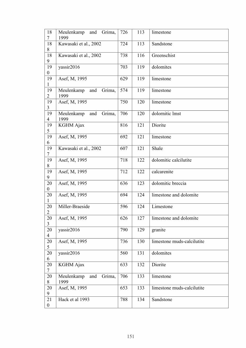
151
18
7
Meulenkamp and Grima,
1999
726 113 limestone
18
8
Kawasaki et al., 2002 724 113 Sandstone
18
9
Kawasaki et al., 2002 738 116 Greenschist
19
0
yassir2016 703 119 dolomites
19
1
Asef, M, 1995 629 119 limestone
19
2
Meulenkamp and Grima,
1999
574 119 limestone
19
3
Asef, M, 1995 750 120 limestone
19
4
Meulenkamp and Grima,
1999
706 120 dolornitic lmst
19
5
KGHM Ajax 816 121 Diorite
19
6
Asef, M, 1995 692 121 limestone
19
7
Kawasaki et al., 2002 607 121 Shale
19
8
Asef, M, 1995 718 122 dolomitic calcilutite
19
9
Asef, M, 1995 712 122 calcarenite
20
0
Asef, M, 1995 636 123 dolomitic breccia
20
1
Asef, M, 1995 694 124 limestone and dolomite
20
2
Miller-Braeside 596 124 Limestone
20
3
Asef, M, 1995 626 127 limestone and dolomite
20
4
yassir2016 790 129 granite
20
5
Asef, M, 1995 736 130 limestone muds-calcilutite
20
6
yassir2016 560 131 dolomites
20
7
KGHM Ajax 633 132 Diorite
20
8
Meulenkamp and Grima,
1999
706 133 limestone
20
9
Asef, M, 1995 653 133 limestone muds-calcilutite
21
0
Hack et al 1993 788 134 Sandstone

152
21
1
Cobre Del Mayo 757 134 Porphyry
21
2
Cobre Del Mayo 756 134 Porphyry
21
3
RoxGold 716 134 Granite
21
4
Asef, M, 1995 851 135 limestone
21
5
NW Zone PFS 744 135 Metavolcanics
21
6
Kawasaki et al., 2002 712 135 Sandstone
21
7
Asef, M, 1995 780 136 limestone and dolomite
21
8
KGHM Ajax 668 136 Volcanics
21
9
Meulenkamp and Grima,
1999
614 136 limestone
22
0
Meulenkamp and Grima,
1999
713 138 limestone
22
1
Hack et al 1993 634 138 granite
22
2
Hack et al 1993 838 139 granite
22
3
Asef, M, 1995 703 140 limestone muds-calcilutite
22
4
Asef, M, 1995 788 142 dolomitic limestone
22
5
Verwaal and Mulder, 1993 714 142 Sandstone
22
6
Meulenkamp and Grima,
1999
689 142 limestone
22
7
Asef, M, 1995 707 144 dolomitic limestone
22
8
Kawasaki et al., 2002 869 149 Granite
22
9
Hack et al 1993 819 149 Sandstone
23
0
Hack et al 1993 890 151 granite
23
1
RoxGold 753 151 Granite
23
2
NW Zone PFS 856 152 Metavolcanics
23
3
Kawasaki et al., 2002 811 152 Granite
23
4
Aoki and Matsukura, 2007 852 153 Gabrro

153
23
5
Asef, M, 1995 678 154 dolomitic breccia
23
6
KGHM Ajax 863 155 Volcanics
23
7
Hack et al 1993 807 155 granite
23
8
Verwaal and Mulder, 1993 801 155 granite
23
9
Kawasaki et al., 2002 616 155 Granite
24
0
Asef, M, 1995 874 159 limestone
24
1
Verwaal and Mulder, 1993 707 159 Limestone
24
2
RoxGold 696 159 Granite
24
3
Asef, M, 1995 685 160 limestone
24
4
Asef, M, 1995 681 160 limestone-calcarenite layers
24
5
Asef, M, 1995 643 160 limestone muds-calcilutite
24
6
Asef, M, 1995 818 161 limestone muds-calcilutite
24
7
Hack et al 1993 713 161 granite
24
8
Meulenkamp and Grima,
1999
739 162 limestone
24
9
Meulenkamp and Grima,
1999
723 162 limestone
25
0
Aoki and Matsukura, 2007 872 163 Granite
25
1
Meulenkamp and Grima,
1999
862 163 limestone
25
2
Verwaal and Mulder, 1993 751 163 Limestone
25
3
Hack et al 1993 687 163 granite
25
4
NW Zone PFS 812 165 Metavolcanics
25
5
Kawasaki et al., 2002 728 166 Sandstone
25
6
Asef, M, 1995 722 168 dolomitic breccia
25
7
Meulenkamp and Grima,
1999
844 169 limestone
25
8
NW Zone PFS 720 169 Metavolcanics

154
25
9
NW Zone PFS 771 172 Metavolcanics
26
0
Asef, M, 1995 701 173 limestone muds-calcilutite
26
1
Asef, M, 1995 865 174 limestone
26
2
Hack et al 1993 643 174 granite
26
3
Verwaal and Mulder, 1993 640 174 Limestone
26
4
Aoki and Matsukura, 2007 853 175 Granite
26
5
Asef, M, 1995 664 175 limestone muds-calcilutite
26
6
Hack et al 1993 685 176 Limestone
26
7
Verwaal and Mulder, 1993 653 176 Limestone
26
8
Hack et al 1993 856 178 granite
26
9
KGHM Ajax 712 178 Volcanics
27
0
Kawasaki et al., 2002 596 178 Sandstone
27
1
Kawasaki et al., 2002 782 179 Sandstone
27
2
Kawasaki et al., 2002 732 179 Sandstone
27
3
Hack et al 1993 721 181 Limestone
27
4
Hack et al 1993 695 181 Limestone
27
5
Asef, M, 1995 711 182 dolomitic limestone
27
6
Hack et al 1993 561 182 Limestone
27
7
Verwaal and Mulder, 1993 705 183 Limestone
27
8
Verwaal and Mulder, 1993 688 186 Limestone
27
9
Hack et al 1993 798 187 Limestone
28
0
Meulenkamp and Grima,
1999
710 187 granite
28
1
Asef, M, 1995 909 188 limestone muds-calcilutite
28
2
RoxGold 656 188 Felsic Dyke
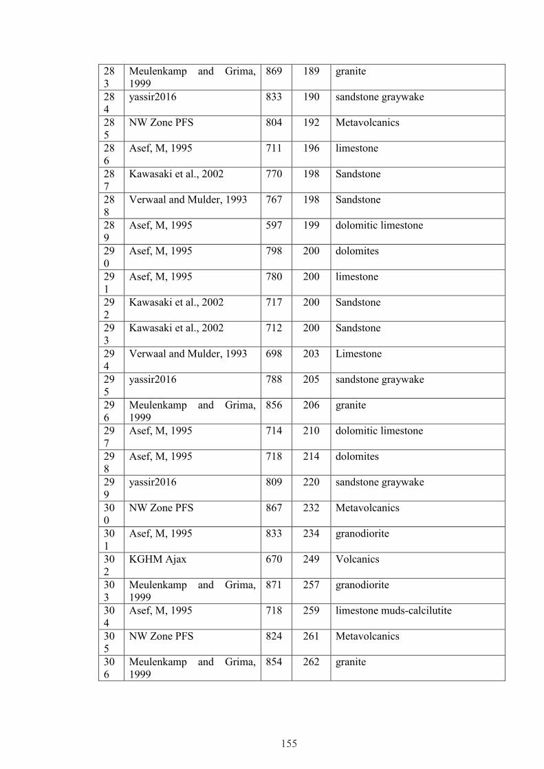
155
28
3
Meulenkamp and Grima,
1999
869 189 granite
28
4
yassir2016 833 190 sandstone graywake
28
5
NW Zone PFS 804 192 Metavolcanics
28
6
Asef, M, 1995 711 196 limestone
28
7
Kawasaki et al., 2002 770 198 Sandstone
28
8
Verwaal and Mulder, 1993 767 198 Sandstone
28
9
Asef, M, 1995 597 199 dolomitic limestone
29
0
Asef, M, 1995 798 200 dolomites
29
1
Asef, M, 1995 780 200 limestone
29
2
Kawasaki et al., 2002 717 200 Sandstone
29
3
Kawasaki et al., 2002 712 200 Sandstone
29
4
Verwaal and Mulder, 1993 698 203 Limestone
29
5
yassir2016 788 205 sandstone graywake
29
6
Meulenkamp and Grima,
1999
856 206 granite
29
7
Asef, M, 1995 714 210 dolomitic limestone
29
8
Asef, M, 1995 718 214 dolomites
29
9
yassir2016 809 220 sandstone graywake
30
0
NW Zone PFS 867 232 Metavolcanics
30
1
Asef, M, 1995 833 234 granodiorite
30
2
KGHM Ajax 670 249 Volcanics
30
3
Meulenkamp and Grima,
1999
871 257 granodiorite
30
4
Asef, M, 1995 718 259 limestone muds-calcilutite
30
5
NW Zone PFS 824 261 Metavolcanics
30
6
Meulenkamp and Grima,
1999
854 262 granite
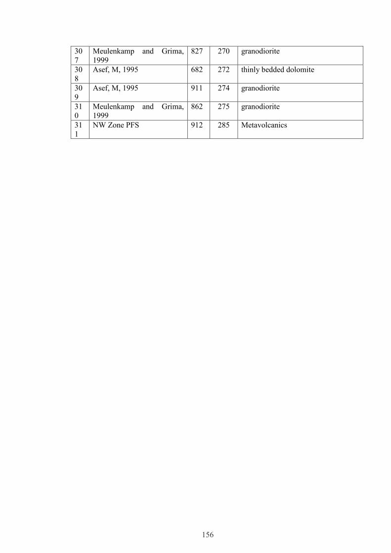
156
30
7
Meulenkamp and Grima,
1999
827 270 granodiorite
30
8
Asef, M, 1995 682 272 thinly bedded dolomite
30
9
Asef, M, 1995 911 274 granodiorite
31
0
Meulenkamp and Grima,
1999
862 275 granodiorite
31
1
NW Zone PFS 912 285 Metavolcanics

157
Sandstone datapoints (UCS - HLD correlation)
HLD UCS (MPa) Fits CI lower CI upper
809 220 197 177 217
788 205 175 160 191
798 200 186 168 203
780 200 168 154 183
770 198 159 146 172
767 198 157 145 170
833 190 224 197 250
782 179 170 156 185
732 179 130 120 140
712 178 117 107 127
728 166 127 117 138
819 149 208 186 231
788 142 176 160 191
744 135 139 128 150
756 134 148 137 160
726 113 126 116 136
612 102 68 57 79
631 92 76 65 87
714 92 118 108 128
658 88 87 77 98
620 82 71 60 82
536 82 45 35 56
538 80 46 35 57
606 77 66 55 77
667 76 92 82 102
545 76 48 37 58
668 74 92 82 103
666 74 91 81 102
654 74 86 75 96
646 74 82 71 93
649 73 83 73 94
622 72 72 61 83
627 59 74 63 85
576 52 56 45 67
482 52 34 24 44
574 51 56 45 67
642 40 80 69 91
595 38 62 51 73
591 37 61 50 72

158
HLD UCS (MPa) Fits CI lower CI upper
659 37 88 77 98
591 35 61 50 72
677 35 97 86 107
412 31 23 15 32
316 15 14 7 20
450 15 29 19 38
Igneous datapoints (UCS - HLD correlation)
HLD UCS (MPa) Fits CI lower CI upper
827 270 170 156 184
854 262 182 166 199
871 257 190 171 209
869 189 189 171 208
862 275 186 168 203
856 206 183 166 200
798 187 158 144 171
409 16 38 19 56
644 60 100 82 118
872 163 191 172 209
853 175 182 165 198
485 64 54 34 74
852 153 181 165 198
807 155 161 148 175
487 18 55 35 75
558 54 73 53 93
630 52 95 77 113
716 134 125 110 140
757 134 141 127 154
684 88 113 97 130
874 159 191 172 211
788 95 153 140 166
788 134 153 140 166
909 188 208 184 233
890 151 199 178 220
646 75 100 82 118
642 80 99 81 117
576 72 78 59 98
681 106 112 96 129
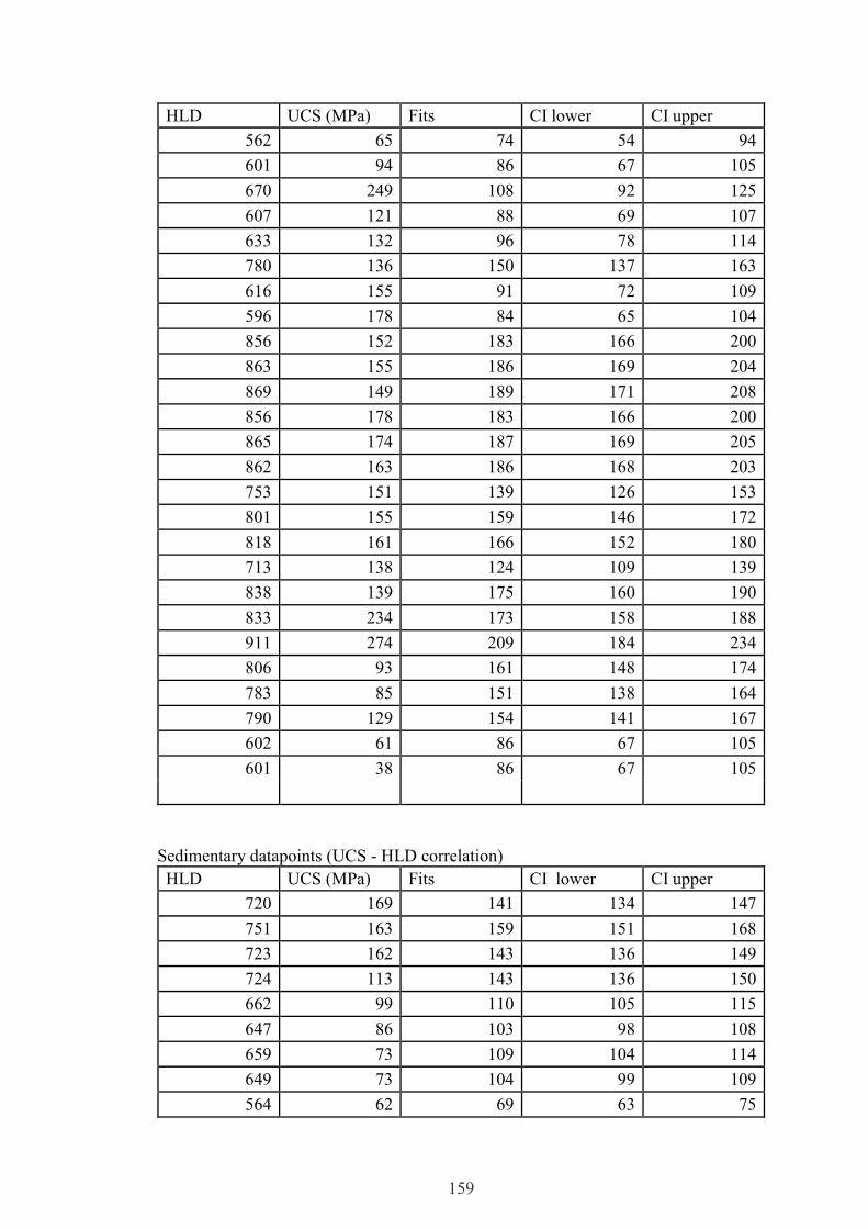
159
HLD UCS (MPa) Fits CI lower CI upper
562 65 74 54 94
601 94 86 67 105
670 249 108 92 125
607 121 88 69 107
633 132 96 78 114
780 136 150 137 163
616 155 91 72 109
596 178 84 65 104
856 152 183 166 200
863 155 186 169 204
869 149 189 171 208
856 178 183 166 200
865 174 187 169 205
862 163 186 168 203
753 151 139 126 153
801 155 159 146 172
818 161 166 152 180
713 138 124 109 139
838 139 175 160 190
833 234 173 158 188
911 274 209 184 234
806 93 161 148 174
783 85 151 138 164
790 129 154 141 167
602 61 86 67 105
601 38 86 67 105
Sedimentary datapoints (UCS - HLD correlation)
HLD UCS (MPa) Fits CI lower CI upper
720 169 141 134 147
751 163 159 151 168
723 162 143 136 149
724 113 143 136 150
662 99 110 105 115
647 86 103 98 108
659 73 109 104 114
649 73 104 99 109
564 62 69 63 75
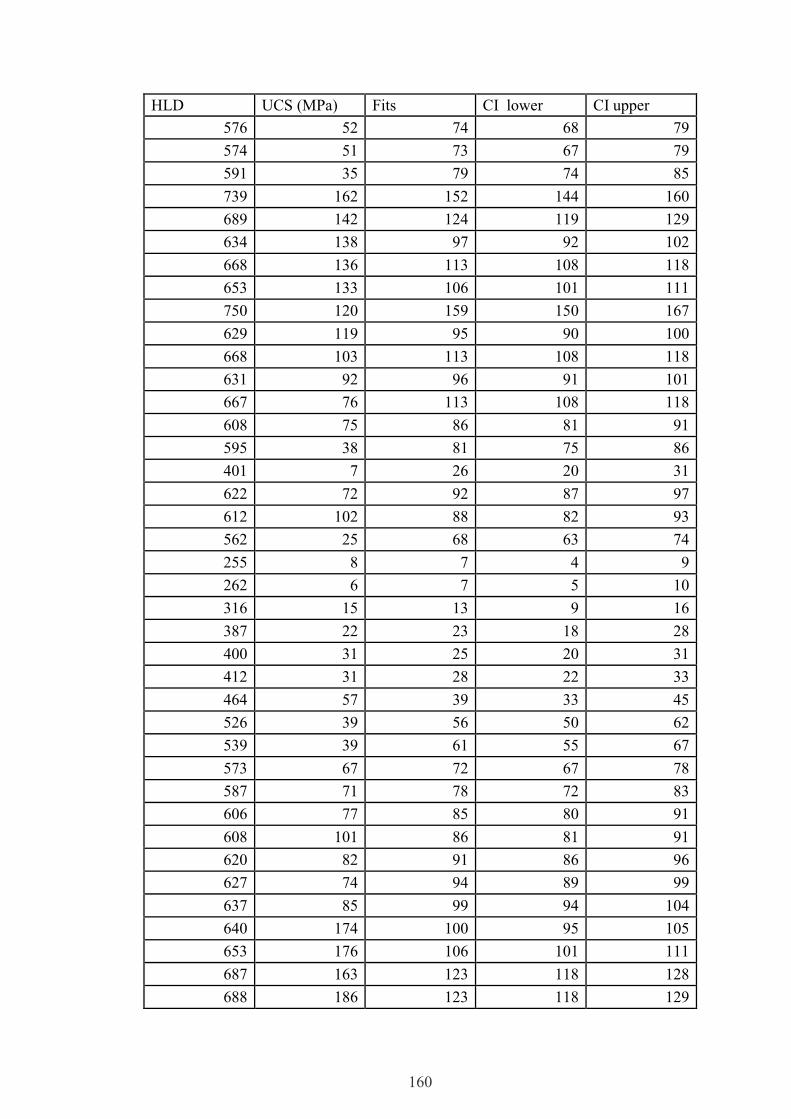
160
HLD UCS (MPa) Fits CI lower CI upper
576 52 74 68 79
574 51 73 67 79
591 35 79 74 85
739 162 152 144 160
689 142 124 119 129
634 138 97 92 102
668 136 113 108 118
653 133 106 101 111
750 120 159 150 167
629 119 95 90 100
668 103 113 108 118
631 92 96 91 101
667 76 113 108 118
608 75 86 81 91
595 38 81 75 86
401 7 26 20 31
622 72 92 87 97
612 102 88 82 93
562 25 68 63 74
255 8 7 4 9
262 6 7 5 10
316 15 13 9 16
387 22 23 18 28
400 31 25 20 31
412 31 28 22 33
464 57 39 33 45
526 39 56 50 62
539 39 61 55 67
573 67 72 67 78
587 71 78 72 83
606 77 85 80 91
608 101 86 81 91
620 82 91 86 96
627 74 94 89 99
637 85 99 94 104
640 174 100 95 105
653 176 106 101 111
687 163 123 118 128
688 186 123 118 129
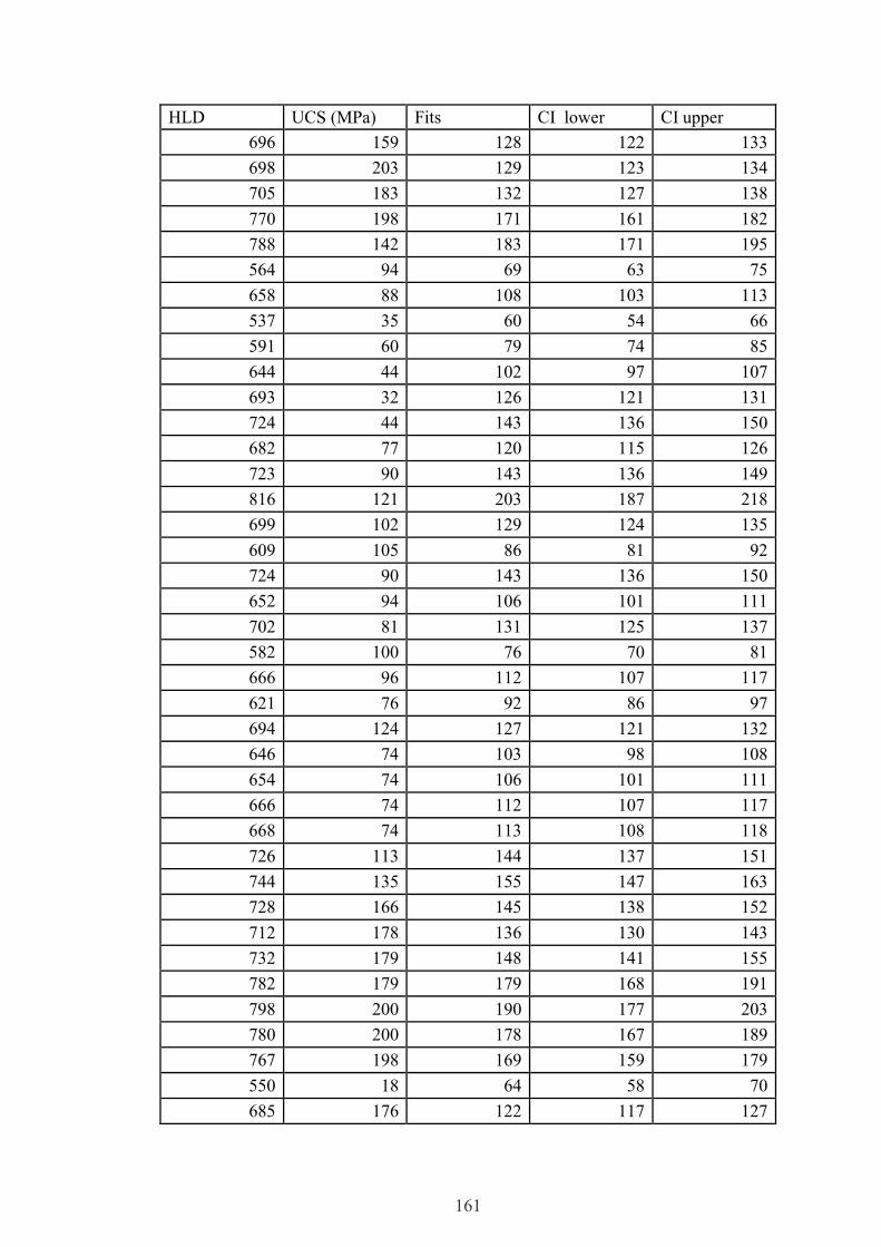
161
HLD UCS (MPa) Fits CI lower CI upper
696 159 128 122 133
698 203 129 123 134
705 183 132 127 138
770 198 171 161 182
788 142 183 171 195
564 94 69 63 75
658 88 108 103 113
537 35 60 54 66
591 60 79 74 85
644 44 102 97 107
693 32 126 121 131
724 44 143 136 150
682 77 120 115 126
723 90 143 136 149
816 121 203 187 218
699 102 129 124 135
609 105 86 81 92
724 90 143 136 150
652 94 106 101 111
702 81 131 125 137
582 100 76 70 81
666 96 112 107 117
621 76 92 86 97
694 124 127 121 132
646 74 103 98 108
654 74 106 101 111
666 74 112 107 117
668 74 113 108 118
726 113 144 137 151
744 135 155 147 163
728 166 145 138 152
712 178 136 130 143
732 179 148 141 155
782 179 179 168 191
798 200 190 177 203
780 200 178 167 189
767 198 169 159 179
550 18 64 58 70
685 176 122 117 127

162
HLD UCS (MPa) Fits CI lower CI upper
695 181 127 122 133
711 182 136 130 142
721 181 141 135 148
710 187 135 129 141
756 134 162 153 171
819 149 205 189 221
536 50 60 54 66
531 51 58 52 64
526 46 56 50 62
555 38 66 60 72
523 44 56 49 62
526 32 56 50 62
547 51 63 57 69
520 65 55 49 61
516 75 53 47 59
504 41 50 44 56
480 55 43 37 49
527 54 57 51 63
515 27 53 47 59
520 56 55 49 61
553 47 65 59 71
511 66 52 46 58
526 55 56 50 62
548 36 64 58 70
582 77 76 70 81
564 78 69 63 75
531 51 58 52 64
576 55 74 68 79
545 64 63 57 69
553 60 65 59 71
466 46 40 34 46
455 35 37 31 43
471 48 41 35 47
532 58 58 52 64
493 68 47 41 53
486 32 45 39 51
472 72 41 35 47
482 65 44 38 50
458 62 38 32 44

163
HLD UCS (MPa) Fits CI lower CI upper
448 33 35 30 41
420 17 29 24 35
447 43 35 29 41
385 27 23 18 28
439 42 33 28 39
473 60 41 35 47
428 66 31 25 37
464 38 39 33 45
495 26 47 41 53
564 77 69 63 75
542 69 62 56 68
500 37 49 43 55
523 55 56 49 62
502 51 49 43 55
501 34 49 43 55
714 210 137 131 144
722 168 142 135 149
692 121 125 120 131
712 122 136 130 143
711 196 136 130 142
575 65 73 67 79
643 174 101 96 106
660 95 109 104 114
636 101 98 93 103
593 57 80 75 86
707 159 134 128 140
385 14 23 18 28
514 24 53 47 59
627 59 94 89 99
545 76 63 57 69
707 144 134 128 140
717 200 139 133 146
714 142 137 131 144
676 66 117 112 122
706 120 133 127 139
718 214 140 133 146
712 200 136 130 143
583 45 76 71 82
712 135 136 130 143
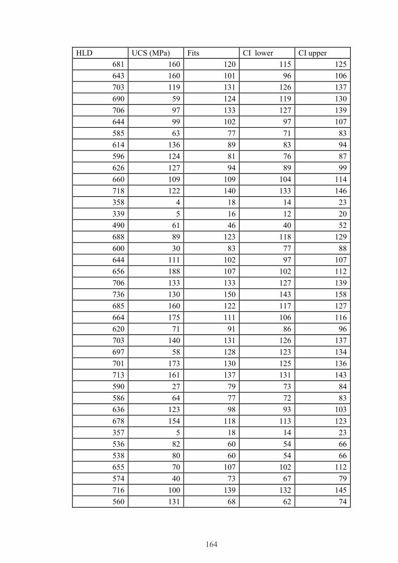
164
HLD UCS (MPa) Fits CI lower CI upper
681 160 120 115 125
643 160 101 96 106
703 119 131 126 137
690 59 124 119 130
706 97 133 127 139
644 99 102 97 107
585 63 77 71 83
614 136 89 83 94
596 124 81 76 87
626 127 94 89 99
660 109 109 104 114
718 122 140 133 146
358 4 18 14 23
339 5 16 12 20
490 61 46 40 52
688 89 123 118 129
600 30 83 77 88
644 111 102 97 107
656 188 107 102 112
706 133 133 127 139
736 130 150 143 158
685 160 122 117 127
664 175 111 106 116
620 71 91 86 96
703 140 131 126 137
697 58 128 123 134
701 173 130 125 136
713 161 137 131 143
590 27 79 73 84
586 64 77 72 83
636 123 98 93 103
678 154 118 113 123
357 5 18 14 23
536 82 60 54 66
538 80 60 54 66
655 70 107 102 112
574 40 73 67 79
716 100 139 132 145
560 131 68 62 74

165
HLD UCS (MPa) Fits CI lower CI upper
593 66 80 75 86
574 119 73 67 79
809 220 198 183 212
788 205 183 171 195
833 190 215 198 233
Metamorphic datapoints (UCS - HLD correlation)
HLD UCS (MPa) Fits CI lower CI upper
603 94 43 32 53
265 13 5 2 9
274 15 6 2 9
324 3 8 3 12
377 6 11 5 16
470 12 19 11 27
514 34 25 16 33
564 27 34 24 43
695 45 74 63 86
738 116 96 85 108
669 78 63 52 75
655 72 58 47 70
464 48 18 11 26
670 51 64 52 76
694 58 74 62 86
662 46 61 49 72
609 67 44 33 55
642 59 54 43 65
762 101 112 100 123
767 111 115 103 126
786 81 129 117 141
763 94 112 101 124
790 77 132 120 144
570 28 35 25 45
689 69 72 60 83
771 172 118 106 129
476 18 20 12 27
811 152 150 137 163
659 62 60 48 71
795 90 136 124 148
844 169 183 166 200
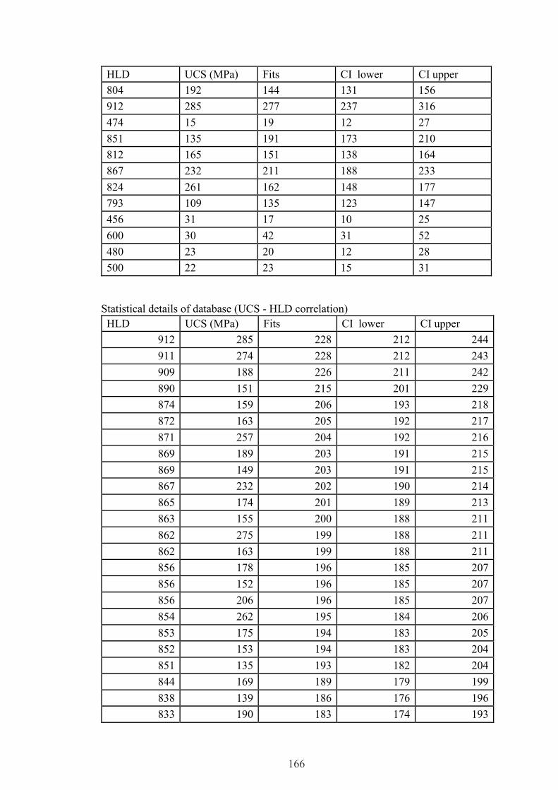
166
HLD UCS (MPa) Fits CI lower CI upper
804 192 144 131 156
912 285 277 237 316
474 15 19 12 27
851 135 191 173 210
812 165 151 138 164
867 232 211 188 233
824 261 162 148 177
793 109 135 123 147
456 31 17 10 25
600 30 42 31 52
480 23 20 12 28
500 22 23 15 31
Statistical details of database (UCS - HLD correlation)
HLD UCS (MPa) Fits CI lower CI upper
912 285 228 212 244
911 274 228 212 243
909 188 226 211 242
890 151 215 201 229
874 159 206 193 218
872 163 205 192 217
871 257 204 192 216
869 189 203 191 215
869 149 203 191 215
867 232 202 190 214
865 174 201 189 213
863 155 200 188 211
862 275 199 188 211
862 163 199 188 211
856 178 196 185 207
856 152 196 185 207
856 206 196 185 207
854 262 195 184 206
853 175 194 183 205
852 153 194 183 204
851 135 193 182 204
844 169 189 179 199
838 139 186 176 196
833 190 183 174 193
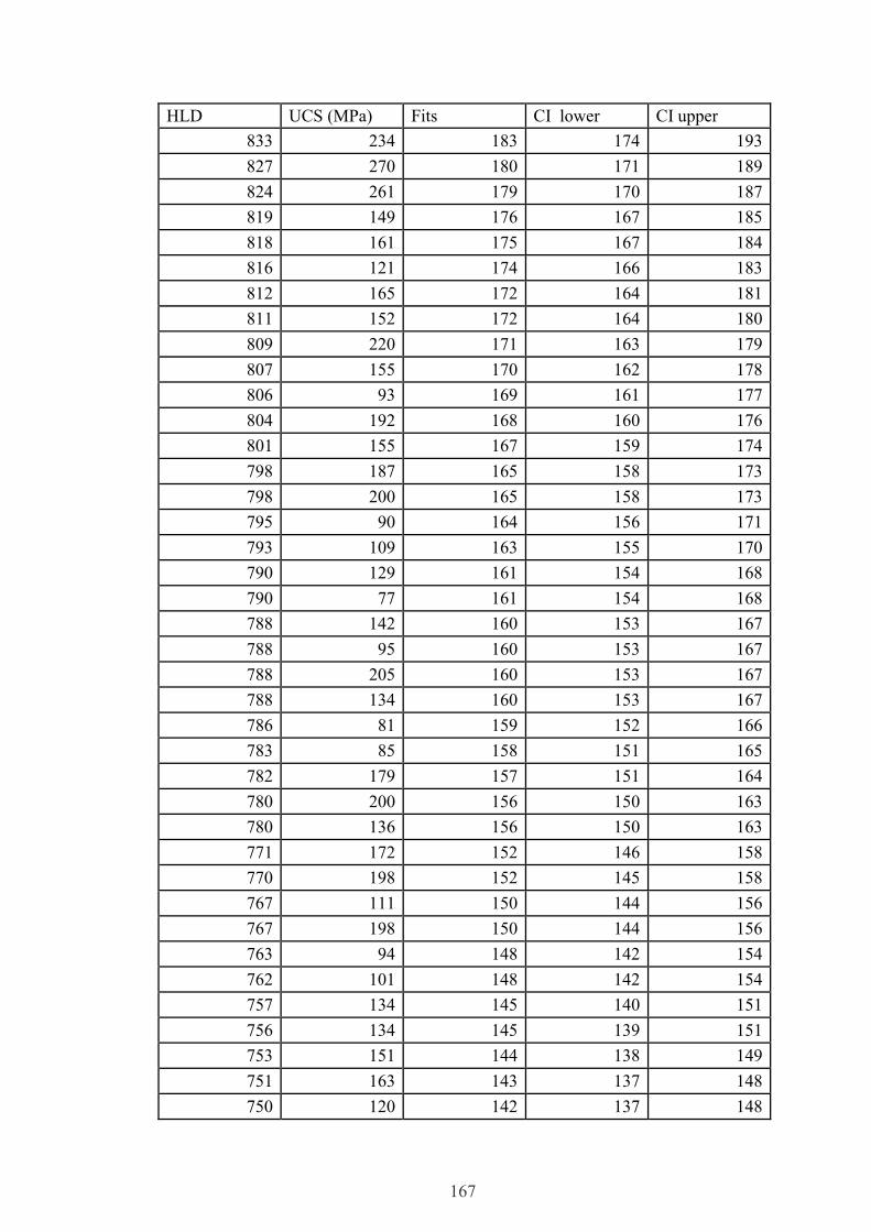
167
HLD UCS (MPa) Fits CI lower CI upper
833 234 183 174 193
827 270 180 171 189
824 261 179 170 187
819 149 176 167 185
818 161 175 167 184
816 121 174 166 183
812 165 172 164 181
811 152 172 164 180
809 220 171 163 179
807 155 170 162 178
806 93 169 161 177
804 192 168 160 176
801 155 167 159 174
798 187 165 158 173
798 200 165 158 173
795 90 164 156 171
793 109 163 155 170
790 129 161 154 168
790 77 161 154 168
788 142 160 153 167
788 95 160 153 167
788 205 160 153 167
788 134 160 153 167
786 81 159 152 166
783 85 158 151 165
782 179 157 151 164
780 200 156 150 163
780 136 156 150 163
771 172 152 146 158
770 198 152 145 158
767 111 150 144 156
767 198 150 144 156
763 94 148 142 154
762 101 148 142 154
757 134 145 140 151
756 134 145 139 151
753 151 144 138 149
751 163 143 137 148
750 120 142 137 148
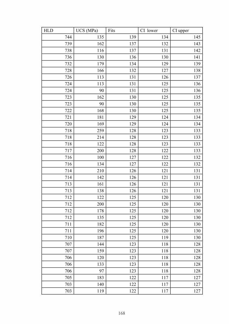
168
HLD UCS (MPa) Fits CI lower CI upper
744 135 139 134 145
739 162 137 132 143
738 116 137 131 142
736 130 136 130 141
732 179 134 129 139
728 166 132 127 138
726 113 131 126 137
724 113 131 125 136
724 90 131 125 136
723 162 130 125 135
723 90 130 125 135
722 168 130 125 135
721 181 129 124 134
720 169 129 124 134
718 259 128 123 133
718 214 128 123 133
718 122 128 123 133
717 200 128 122 133
716 100 127 122 132
716 134 127 122 132
714 210 126 121 131
714 142 126 121 131
713 161 126 121 131
713 138 126 121 131
712 122 125 120 130
712 200 125 120 130
712 178 125 120 130
712 135 125 120 130
711 182 125 120 130
711 196 125 120 130
710 187 125 119 130
707 144 123 118 128
707 159 123 118 128
706 120 123 118 128
706 133 123 118 128
706 97 123 118 128
705 183 122 117 127
703 140 122 117 127
703 119 122 117 127
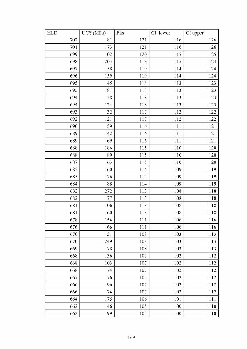
169
HLD UCS (MPa) Fits CI lower CI upper
702 81 121 116 126
701 173 121 116 126
699 102 120 115 125
698 203 119 115 124
697 58 119 114 124
696 159 119 114 124
695 45 118 113 123
695 181 118 113 123
694 58 118 113 123
694 124 118 113 123
693 32 117 112 122
692 121 117 112 122
690 59 116 111 121
689 142 116 111 121
689 69 116 111 121
688 186 115 110 120
688 89 115 110 120
687 163 115 110 120
685 160 114 109 119
685 176 114 109 119
684 88 114 109 119
682 272 113 108 118
682 77 113 108 118
681 106 113 108 118
681 160 113 108 118
678 154 111 106 116
676 66 111 106 116
670 51 108 103 113
670 249 108 103 113
669 78 108 103 113
668 136 107 102 112
668 103 107 102 112
668 74 107 102 112
667 76 107 102 112
666 96 107 102 112
666 74 107 102 112
664 175 106 101 111
662 46 105 100 110
662 99 105 100 110

170
HLD UCS (MPa) Fits CI lower CI upper
660 109 104 99 109
660 95 104 99 109
659 73 104 99 109
659 62 104 99 109
658 88 104 99 109
656 188 103 98 108
655 70 102 97 108
655 72 102 97 108
654 74 102 97 107
653 176 102 97 107
653 133 102 97 107
652 94 101 96 106
649 73 100 95 105
647 86 99 94 105
646 75 99 94 104
646 74 99 94 104
644 99 98 93 103
644 60 98 93 103
644 111 98 93 103
644 44 98 93 103
643 174 98 93 103
643 160 98 93 103
642 80 98 92 103
642 59 98 92 103
640 174 97 92 102
637 85 96 91 101
636 123 95 90 101
636 101 95 90 101
634 138 95 89 100
633 132 94 89 100
631 92 94 88 99
630 52 93 88 98
629 119 93 88 98
627 74 92 87 97
627 59 92 87 97
626 127 92 87 97
622 72 90 85 96
621 76 90 85 95
620 82 90 84 95

171
HLD UCS (MPa) Fits CI lower CI upper
620 71 90 84 95
616 155 88 83 94
614 136 88 82 93
612 102 87 82 92
609 105 86 80 91
609 67 86 80 91
608 101 86 80 91
608 75 86 80 91
607 121 85 80 91
606 77 85 79 90
603 94 84 78 89
602 61 84 78 89
601 94 83 78 89
601 38 83 78 89
600 30 83 77 88
600 30 83 77 88
597 199 82 76 87
596 178 82 76 87
596 124 82 76 87
595 38 81 76 87
593 57 81 75 86
593 66 81 75 86
591 35 80 74 85
591 60 80 74 85
590 27 80 74 85
587 71 79 73 84
586 64 78 73 84
585 63 78 72 84
583 45 77 72 83
582 100 77 71 83
582 77 77 71 83
576 52 75 69 81
576 72 75 69 81
576 55 75 69 81
575 65 75 69 80
574 119 74 69 80
574 51 74 69 80
574 40 74 69 80
573 67 74 68 80

172
HLD UCS (MPa) Fits CI lower CI upper
570 28 73 68 79
564 62 71 66 77
564 78 71 66 77
564 77 71 66 77
564 27 71 66 77
564 94 71 66 77
562 25 71 65 76
562 65 71 65 76
562 26 71 65 76
561 182 70 65 76
560 131 70 64 76
558 54 70 64 75
555 38 69 63 74
553 60 68 62 74
553 47 68 62 74
550 18 67 61 73
548 36 67 61 72
547 51 66 61 72
545 76 66 60 71
545 64 66 60 71
542 69 65 59 71
539 39 64 58 70
538 80 64 58 69
537 35 63 58 69
536 82 63 57 69
536 50 63 57 69
532 58 62 56 68
531 51 62 56 67
531 51 62 56 67
527 54 61 55 66
526 55 60 54 66
526 46 60 54 66
526 39 60 54 66
526 32 60 54 66
523 55 59 54 65
523 44 59 54 65
520 65 59 53 64
520 56 59 53 64
516 75 58 52 63

173
HLD UCS (MPa) Fits CI lower CI upper
515 27 57 51 63
514 34 57 51 63
514 24 57 51 63
511 66 56 50 62
504 41 54 49 60
502 51 54 48 60
501 34 54 48 59
500 37 53 48 59
500 22 53 48 59
495 26 52 46 58
493 68 52 46 57
490 61 51 45 57
487 18 50 44 56
486 32 50 44 56
485 64 50 44 55
482 65 49 43 55
480 55 48 43 54
480 23 48 43 54
476 18 47 42 53
474 15 47 41 53
473 60 47 41 52
472 72 46 41 52
471 48 46 40 52
470 12 46 40 52
466 46 45 39 51
464 57 44 39 50
464 38 44 39 50
464 48 44 39 50
458 62 43 38 49
456 31 43 37 48
455 35 42 37 48
448 33 41 35 46
447 43 41 35 46
439 42 39 33 44
428 66 37 31 42
420 17 35 30 40
412 31 33 28 39
409 16 33 28 38
401 7 31 26 36

174
HLD UCS (MPa) Fits CI lower CI upper
400 31 31 26 36
387 22 29 24 34
385 14 28 23 33
385 27 28 23 33
377 6 27 22 32
358 4 24 19 28
357 5 24 19 28
339 5 21 17 25
324 3 19 15 23
316 15 18 14 22
274 15 12 9 16
265 13 11 8 15
262 6 11 8 14
255 8 10 8 13
Related Documents


