by Christian Ahlin and Robert Townsend

SELECTION INTO AND ACROSS CREDIT CONTRACTS:THEORY AND FIELD RESEARCH

by

Christian Ahlin and Robert Townsend

Working Paper No. 03-W23

October 2003

DEPARTMENT OF ECONOMICSVANDERBILT UNIVERSITY

NASHVILLE, TN 37235

www.vanderbilt.edu/econ

Selection into and across Credit Contracts:Theory and Field Research

Christian Ahlin and Robert Townsend∗

October 2003

Abstract

Various theories make predictions about the relative advantages of individual loansversus joint liability loans. If we imagine that lenders facing moral hazard make relativeperformance comparisons in determining stringency in repayment, then individual loansshould vary positively with covariance of output across funded projects. Relativelynew work also highlights inequality and heterogeneity in preferences, establishing thatwealth of the agents relative to the bank, and wealth dispersion among potential jointliability partners, are important factors determining the likelihood of the joint liabilityregime. An alternative imperfect information model also addresses the question ofwhich agents will accept a group contract and borrow and which will pursue outsideoptions. We attempt to test these various models using relatively rich data gatheredin field research in Thailand, measuring not only the presence of joint liability versusindividual loans, but also measuring various of the key variables suggested by thesetheories. As predicted by one of the theories, the prevalence of joint liability contractsrelative to individual contracts exhibits a U-shaped relationship with the wealth ofthe borrowing pair and increases with the wealth dispersion. (We control for wealththat can be used as collateral.) Contrary to one theory, we find no evidence jointliability borrowing becomes less likely as covariance of output increases. We do find,consistent with our modified version of the model with adverse selection, that highercorrelation makes joint liability borrowing more likely relative to all outside options.We also find direct evidence consistent with adverse selection in the credit market, inthat the likelihood of joint-liability borrowing increases the lower is the probability ofproject success. We are able to distinguish this result from an alternative moral hazardexplanation. Strikingly, most of the results disappear if we do not condition the sampleaccording to the dictates of the models.

∗We thank Eric Bond, William Collins, Bernard Salanie, and seminar participants at Chicago, Vander-bilt, Stanford Institute for Theoretical Economics, and Yale for helpful comments. Financial support fromthe National Institute of Health and the National Science Foundation (including its Graduate ResearchFellowship Program) is gratefully acknowledged. All errors are ours.

1

1 Introduction

The literature on micro credit as a major tool against world poverty is polarized over thedebate of the virtues of individual versus group, joint liability lending. For the most part,only one contract per lender is observed, e.g., group lending under the Grameen Bank inBangladesh and individual loans under BRI in Indonesia. It is thus difficult to make progressin the debate. We do not see what would happen if the alternative contract were available,not to mention all the difficulties inherent in cross country comparisons. Here we takeadvantage of the menu of contracts offered by a dominant rural lender in a single country andsome unusual data gathered in field research to make some headway on the issue. Potentialborrowers from the BAAC1 in Thailand decide whether to borrow at all, and if so, whetherto borrow as individuals or under joint liability. That is, potential borrowers select into andacross loan contracts. There is in fact much variation in these choices in the data. We thususe the data to test various well-known models from the contract theory, mechanism designliterature.

One interpretation of group loans is as a way for the lender to encourage trade, or con-tracting, between the borrowers. Group loans are accompanied by required group meetingsand explicit group-related contingencies. They are also formed mostly autonomously bygroup members themselves. This kind of lending arrangement would seem to facilitate (orindeed encourage) contracting among the borrowers. The advantage of such interactionwould be enhanced ability to monitor and enforce intra-group agreements on actions andtransfers (i.e. risk sharing). The downside of such interaction is the ability to collude againstthe lender, coordinating in the choice of low mutual effort or reallocating internal resources(e.g., tunneling). Under individual loans, without collusion, the lender can gage if one bor-rower has been diligent by looking to see if other individual borrowers are doing well. Underthis interpretation of group and individual loans, it is not obvious the kind of loan for whichmoral hazard considerations argue.

Indeed theories of individual vs. group loans often do not make unequivocal predictions.It has been shown, for example by Holmstrom and Milgrom (1990) (hereafter HM), that aprincipal, or lender, faced with the problem of inducing effort from agents, or borrowers,when effort is imperfectly observed can use correlation between the random component ofborrowers’ returns to mitigate this imperfect information. The higher this technologicalcorrelation, the more effectively is the information problem dealt with in such a relativeperformance regime, and the risk cost of high-powered incentives decreases. This type ofresult relies on the borrowers acting non-cooperatively. If they instead act cooperativelyand are assumed able to honor side-contracts to ensure risk and enforce actions, a relativeperformance regime can be manipulated to lead to adverse results. The lender’s handsare thus tied. However, the ability of the borrowers to coordinate and share risk amongthemselves lowers risk costs and raises total surplus, all else equal. The closer to zero is thecorrelation between the borrowers’ returns, the greater the scope for internal risk sharing. Asintuition suggests and Holmstrom and Milgrom show formally, it would be Pareto optimalfor the borrowers to be acting non-cooperatively if technological correlation is high enough,and cooperatively if it is low enough. In principle, this is a testable implication.

1BAAC is short for the Bank for Agriculture and Agricultural Cooperatives.

2

Prescott and Townsend (1999) (hereafter PT) address similar questions but focus insteadon wealth levels of borrowers relative to the lender and wealth dispersion across borrowers.They offer an extended version of the above-mentioned unobserved effort model, generalizedin several directions, but without closed form solutions available. In simulations, they findthat for asymmetric enough Pareto weights on the two borrowers, interpretable as high wealthdispersion, the cooperative regime dominates. When the weights are more similar, the non-cooperative regime dominates. Apparently the cooperative regime is better at extractingeffort from the low-weight borrower. Further, the cooperative regime dominates for highenough or low enough reservation payoff of the lender, interpretable as the inverse of theborrowers’ wealth, while an intermediate value makes the non-cooperative regime optimal.Again, both these predictions are in principle testable.

Another interpretation, perhaps more common, of a joint liability, group loan is that anindividual borrower promises to repay a lender if able but a second, co-signer of that sameloan promises to repay if the first borrower is unable. Group loans are a version of this inwhich each member of the group is borrowing and jointly liable for the loans of the others.In contrast, under individual liability, the borrower enters into a contract with the lender,potentially offering collateral, and no third parties are directly involved.

Under this interpretation, joint liability loans in conjunction with good local informationon risk types are also thought to help overcome a different problem, adverse selection. Someborrowers are inherently more risky than others. In a setting of limited, individual liabilityand lender ignorance of risk-type, risky borrowers are in effect subsidized by safe ones. Insome instances this cuts out socially productive loans to safe borrowers.2 Joint liability,through homogeneous matching among risk types, can reduce the subsidy from safe to riskyborrowers and thus mitigate (though not necessarily eliminate) the adverse selection problem,drawing back into the market relatively safe borrowers. Fundamental to this argument, ofcourse, is the existence of an adverse selection problem in the credit market, which someargue is negligible in practice due to banks’ ability to collect information and their offeringof other incentives.3

Ghatak (1999) addresses these questions using a model that is our focus here. We modifythis model to introduce correlation in borrower returns and find that borrowers with highercorrelation of returns will self-select into group contracts (a testable proposition). They dothis because correlation raises their payoff of borrowing by lowering the chances of facingliability for their partner’s loan. Ghatak’s model also exhibits the well-known predictionthat in the context of limited liability, the relatively risky agents are the ones who opt toborrow. Ausubel (1999) tests this proposition with data from credit card companies: thosewilling to select into higher interest rates are more likely to default. A parallel insuranceliterature also tests whether households paying for more complete coverage are more likelyto experience the adverse, insured event. (See the literature review in Chiappori and Salonie(2000)). Here we take advantage of measurements of risk type of those who also choose notto borrow and offer a direct test of this prediction of the adverse selection model.

We attempt to test these predictions from the various models about which kinds ofagents will borrow, and under which kinds of contracts, using relatively rich data gathered

2This kind of adverse selection dates back at least to Stiglitz and Weiss (1981).3See Robinson (2001) for example.

3

in field research in Thailand. We link the non-cooperative regime in the theory (of HMand PT) with individual loans in the data, and the cooperative regime in the theory withjoint liability, group loans in the data. The link is imperfect, but this kind of contractvariation is a plausible means the lender can use to encourage or discourage side-contractingand cooperation. When testing Ghatak, individual loans are linked with an outside optionin the theory, and of course group loans are those where there is joint liability.4 We alsohave measures for wealth, wealth dispersion, technological correlation, and the risk of theborrowers, as well as numerous controls.

Our association of the loan types in the theory with analogs in actual practice deservessome elaboration. The Bank for Agriculture and Agricultural Cooperatives (BAAC) is theprimary institutional lender in rural Thailand: for example 64% of the institutional loansin our sample are from the BAAC. The BAAC does offer both individual loans and jointliability loans. Policy dictates that to receive the latter, one must form or join an officialBAAC-registered borrowing group and enter into a joint liability agreement. A box denotingthat the group is the collateral is checked off on the loan form, and sometimes a particu-lar member in the group is named as a cosigner. In contrast, individual loans must beguaranteed by some form of collateral, usually land. However, the BAAC does not readilyforeclose on either kind of loan, i.e. does not always go after the co-signer or confiscateindividual collateral, respectively. This supports the HM and PT interpretation of loan re-payments as output-contingent and the Ghatak assumption that no payment is demandedfrom a borrower whose project fails. Rather, it has in place a risk-contingency system, asdocumented in Townsend and Yaron (2001), for example. Farmers experiencing force ma-jeur events report their difficulties to the local branch and a credit officer visits the village(the farmer and neighboring households) to verify the adverse event. To an approximationthen, information on output, or at least ability to pay, is observable by the lender. The loancan be rescheduled, and in some instances interest and even part of principal forgiven, as ifan insurance indemnity had kicked in. Thus group, and to a significant degree individual,credit contracts are state contingent loan repayment agreements.5 More generally the BAACis well positioned to make relative performance comparisons in deciding what to do aboutrepayment problems.

The BAAC is not the only lender. In our data we have a complete enumeration of loansoutstanding or repaid in the last twelve months, and for each loan the household respondentis asked what if any collateral was used (land title, cosigner, other). Among these are loansfrom village funds, money lenders, commercial banks, and the informal sector. We also testthe models on a larger sample of individual and co-signed loans from institutional lendersother than the BAAC.

To test the implications of the relative performance vs. joint-liability literature, werestrict the sample to those who have had a loan outstanding in the last twelve months from

4Ghatak shows group loans dominate individual loans for those without collateral, sometimes in a Paretosense and always in terms of total surplus. Thus theory suggests individual loans in the data must becollateralized.

5Under the framework of HM and PT individual loans are fully state contingent (subject to moral hazard)while under our interpretation of the Ghatak framework, individual loans are fully backed by physicalcollateral and are not state contingent. The truth is probably between the two extremes. We carry outrobustness checks when we test the models.

4

the BAAC, or another lender, and throw out of the sample those who did not borrow atall. Likewise, to test the adverse selection models of the literature, we focus on the decisionwhether to borrow under joint liability or any alternative (not borrow at all or borrow underindividual liability).6

As predicted by Prescott and Townsend, the prevalence of joint liability contracts relativeto individual contracts exhibits a U-shaped relationship with the wealth of the borrowing pairand increases with the wealth dispersion. The latter result is especially robust. The resultssurface only when we limit the sample to households with either a group or an individualloan, but not both. This is what theory would suggest, since it compares the two types ofcontracts against each other. The results do not appear to be due to a conventional collateraleffect (in which higher wealth enables households to borrow without cosignors); we separateout and control for the subset of wealth that is most commonly used as collateral.

Contrary to the Holmstrom and Milgrom theory, we find no evidence joint liability bor-rowing becomes less likely as covariance of output increases. This is true when restricting thesample only to those with group or individual loans. When we use the full sample, however,as the Ghatak model would dictate, we find some evidence for the opposite. That is, wefind that higher correlation makes joint liability borrowing more likely relative to all outsideoptions, just as our modified version of Ghatak’s model suggests.

Finally, we find direct evidence consistent with the prediction of adverse selection in thecredit market, in that the likelihood of joint-liability borrowing increases the lower is theprobability of project success. This result only appears when the full sample is used. Thusthe more risky households are borrowing. There is as already noted a related theory-basedempirical literature testing for imperfect information in insurance contract, but as Chiappori,Jullien, Salanie and Salanie (2002) emphasize it is difficult to infer if accident probabilitiesincrease for those purchasing more complete coverage because of adverse selection (ex anteselection) or moral hazard (ex post shirking). Here we further restrict our sample to thosewho have borrowed in the last year but are not currently doing so, and find that the adverseselection remains a force in the data.

Strikingly, as alluded to above, most of these results confirming the models predictionsdisappear if we do not condition the sample according to the dictates of the models.

2 Theories and Implications

2.1 Moral Hazard and Technological Correlation

We focus initially on selection across contracts, given that borrowing is taking place. Cor-relation of output across agents is related by Holmstrom and Milgrom (1990), HM, in thecontext of unobserved actions, to the optimality of an individualistic, relative performanceregime vis a vis a cooperative regime. They find that there exists a cutoff technological cor-relation coefficient, call it ρ. For ρ < ρ, the optimal contract employs a cooperative or groupregime; for ρ > ρ, the optimal contract employs a relative performance regime. Thus, oneshould expect to see more of the group regime among agents whose output is less correlated.

6The results are robust to the inclusion of those borrowing as individuals with those borrowing underjoint liability and to their exclusion.

5

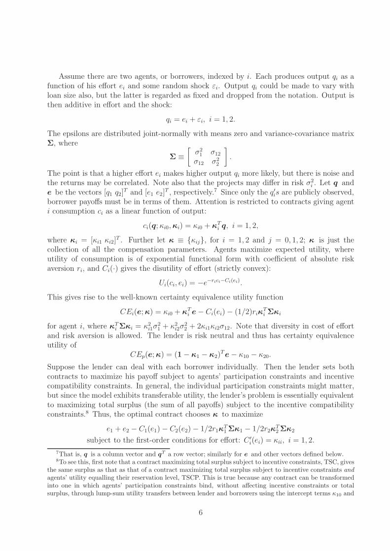
Assume there are two agents, or borrowers, indexed by i. Each produces output qi as afunction of his effort ei and some random shock εi. Output qi could be made to vary withloan size also, but the latter is regarded as fixed and dropped from the notation. Output isthen additive in effort and the shock:

qi = ei + εi, i = 1, 2.

The epsilons are distributed joint-normally with means zero and variance-covariance matrixΣ, where

Σ ≡[

σ21 σ12

σ12 σ22

].

The point is that a higher effort ei makes higher output qi more likely, but there is noise andthe returns may be correlated. Note also that the projects may differ in risk σ2

i . Let q ande be the vectors [q1 q2]

T and [e1 e2]T , respectively.7 Since only the q′is are publicly observed,

borrower payoffs must be in terms of them. Attention is restricted to contracts giving agenti consumption ci as a linear function of output:

ci(q; κi0, κi) = κi0 + κTi q, i = 1, 2,

where κi = [κi1 κi2]T . Further let κ ≡ {κij}, for i = 1, 2 and j = 0, 1, 2; κ is just the

collection of all the compensation parameters. Agents maximize expected utility, whereutility of consumption is of exponential functional form with coefficient of absolute riskaversion ri, and Ci(·) gives the disutility of effort (strictly convex):

Ui(ci, ei) = −e−rici−Ci(ei).

This gives rise to the well-known certainty equivalence utility function

CEi(e; κ) = κi0 + κTi e − Ci(ei) − (1/2)riκ

Ti Σκi

for agent i, where κTi Σκi = κ2

i1σ21 + κ2

i2σ22 + 2κi1κi2σ12. Note that diversity in cost of effort

and risk aversion is allowed. The lender is risk neutral and thus has certainty equivalenceutility of

CEp(e; κ) = (1 − κ1 − κ2)T e − κ10 − κ20.

Suppose the lender can deal with each borrower individually. Then the lender sets bothcontracts to maximize his payoff subject to agents’ participation constraints and incentivecompatibility constraints. In general, the individual participation constraints might matter,but since the model exhibits transferable utility, the lender’s problem is essentially equivalentto maximizing total surplus (the sum of all payoffs) subject to the incentive compatibilityconstraints.8 Thus, the optimal contract chooses κ to maximize

e1 + e2 − C1(e1) − C2(e2) − 1/2r1κT1 Σκ1 − 1/2r2κ

T2 Σκ2

subject to the first-order conditions for effort: C ′i(ei) = κii, i = 1, 2.

7That is, q is a column vector and qT a row vector; similarly for e and other vectors defined below.8To see this, first note that a contract maximizing total surplus subject to incentive constraints, TSC, gives

the same surplus as that as that of a contract maximizing total surplus subject to incentive constraints andagents’ utility equalling their reservation level, TSCP. This is true because any contract can be transformedinto one in which agents’ participation constraints bind, without affecting incentive constraints or totalsurplus, through lump-sum utility transfers between lender and borrowers using the intercept terms κ10 and

6

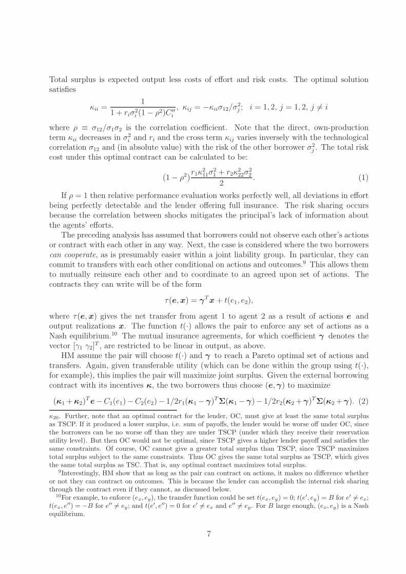
Total surplus is expected output less costs of effort and risk costs. The optimal solutionsatisfies

κii =1

1 + riσ2i (1 − ρ2)C ′′

i

, κij = −κiiσ12/σ2j ; i = 1, 2, j = 1, 2, j �= i

where ρ ≡ σ12/σ1σ2 is the correlation coefficient. Note that the direct, own-productionterm κii decreases in σ2

i and ri and the cross term κij varies inversely with the technologicalcorrelation σ12 and (in absolute value) with the risk of the other borrower σ2

j . The total riskcost under this optimal contract can be calculated to be:

(1 − ρ2)r1κ

211σ

21 + r2κ

222σ

22

2. (1)

If ρ = 1 then relative performance evaluation works perfectly well, all deviations in effortbeing perfectly detectable and the lender offering full insurance. The risk sharing occursbecause the correlation between shocks mitigates the principal’s lack of information aboutthe agents’ efforts.

The preceding analysis has assumed that borrowers could not observe each other’s actionsor contract with each other in any way. Next, the case is considered where the two borrowerscan cooperate, as is presumably easier within a joint liability group. In particular, they cancommit to transfers with each other conditional on actions and outcomes.9 This allows themto mutually reinsure each other and to coordinate to an agreed upon set of actions. Thecontracts they can write will be of the form

τ(e, x) = γT x + t(e1, e2),

where τ(e, x) gives the net transfer from agent 1 to agent 2 as a result of actions e andoutput realizations x. The function t(·) allows the pair to enforce any set of actions as aNash equilibrium.10 The mutual insurance agreements, for which coefficient γ denotes thevector [γ1 γ2]

T , are restricted to be linear in output, as above.HM assume the pair will choose t(·) and γ to reach a Pareto optimal set of actions and

transfers. Again, given transferable utility (which can be done within the group using t(·),for example), this implies the pair will maximize joint surplus. Given the external borrowingcontract with its incentives κ, the two borrowers thus choose (e, γ) to maximize

(κ1 + κ2)T e−C1(e1)−C2(e2)− 1/2r1(κ1 −γ)TΣ(κ1 −γ)− 1/2r2(κ2 +γ)TΣ(κ2 +γ). (2)

κ20. Further, note that an optimal contract for the lender, OC, must give at least the same total surplusas TSCP. If it produced a lower surplus, i.e. sum of payoffs, the lender would be worse off under OC, sincethe borrowers can be no worse off than they are under TSCP (under which they receive their reservationutility level). But then OC would not be optimal, since TSCP gives a higher lender payoff and satisfies thesame constraints. Of course, OC cannot give a greater total surplus than TSCP, since TSCP maximizestotal surplus subject to the same constraints. Thus OC gives the same total surplus as TSCP, which givesthe same total surplus as TSC. That is, any optimal contract maximizes total surplus.

9Interestingly, HM show that as long as the pair can contract on actions, it makes no difference whetheror not they can contract on outcomes. This is because the lender can accomplish the internal risk sharingthrough the contract even if they cannot, as discussed below.

10For example, to enforce (ex, ey), the transfer function could be set t(ex, ey) = 0; t(e′, ey) = B for e′ �= ex;t(ex, e′′) = −B for e′′ �= ey; and t(e′, e′′) = 0 for e′ �= ex and e′′ �= ey. For B large enough, (ex, ey) is a Nashequilibrium.

7

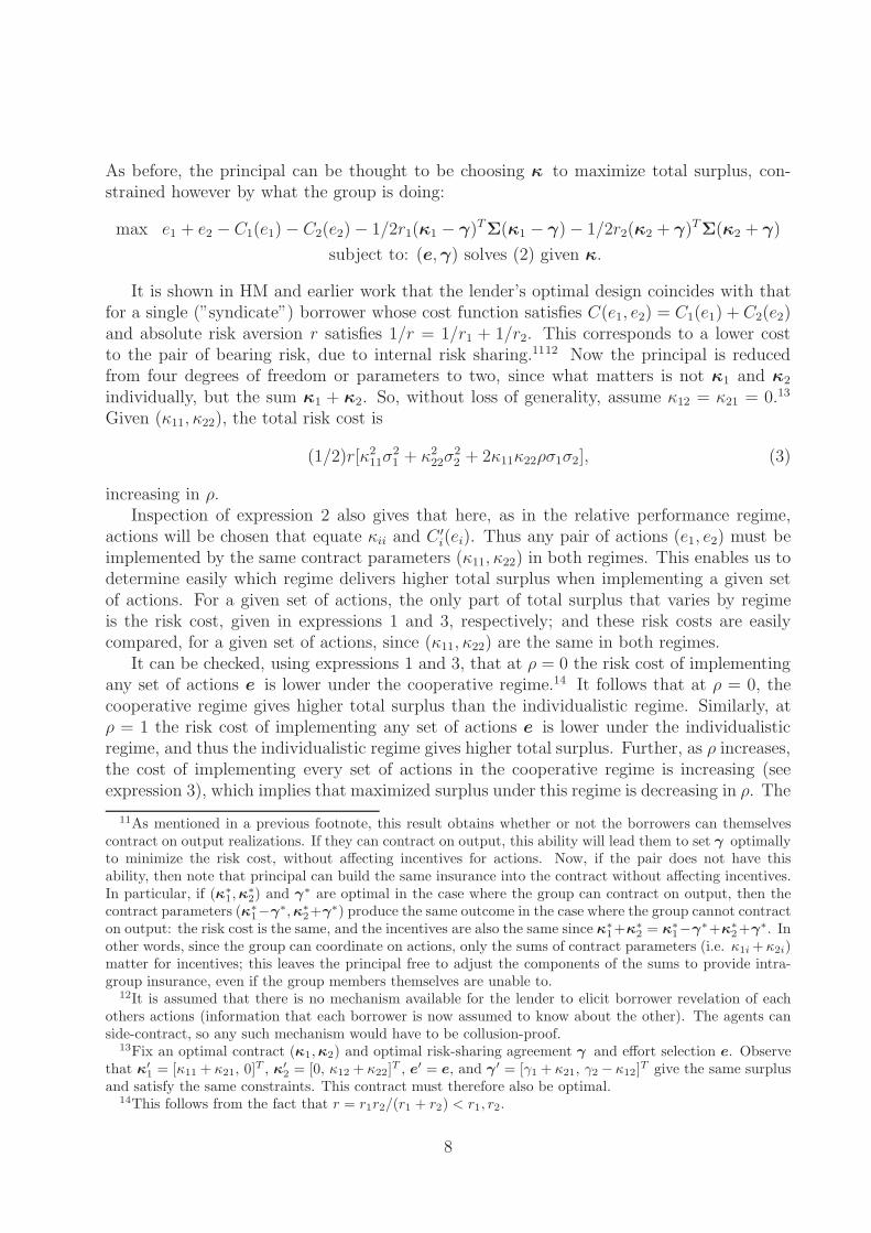
As before, the principal can be thought to be choosing κ to maximize total surplus, con-strained however by what the group is doing:

max e1 + e2 − C1(e1) − C2(e2) − 1/2r1(κ1 − γ)TΣ(κ1 − γ) − 1/2r2(κ2 + γ)TΣ(κ2 + γ)

subject to: (e, γ) solves (2) given κ.

It is shown in HM and earlier work that the lender’s optimal design coincides with thatfor a single (”syndicate”) borrower whose cost function satisfies C(e1, e2) = C1(e1) + C2(e2)and absolute risk aversion r satisfies 1/r = 1/r1 + 1/r2. This corresponds to a lower costto the pair of bearing risk, due to internal risk sharing.1112 Now the principal is reducedfrom four degrees of freedom or parameters to two, since what matters is not κ1 and κ2

individually, but the sum κ1 + κ2. So, without loss of generality, assume κ12 = κ21 = 0.13

Given (κ11, κ22), the total risk cost is

(1/2)r[κ211σ

21 + κ2

22σ22 + 2κ11κ22ρσ1σ2], (3)

increasing in ρ.Inspection of expression 2 also gives that here, as in the relative performance regime,

actions will be chosen that equate κii and C ′i(ei). Thus any pair of actions (e1, e2) must be

implemented by the same contract parameters (κ11, κ22) in both regimes. This enables us todetermine easily which regime delivers higher total surplus when implementing a given setof actions. For a given set of actions, the only part of total surplus that varies by regimeis the risk cost, given in expressions 1 and 3, respectively; and these risk costs are easilycompared, for a given set of actions, since (κ11, κ22) are the same in both regimes.

It can be checked, using expressions 1 and 3, that at ρ = 0 the risk cost of implementingany set of actions e is lower under the cooperative regime.14 It follows that at ρ = 0, thecooperative regime gives higher total surplus than the individualistic regime. Similarly, atρ = 1 the risk cost of implementing any set of actions e is lower under the individualisticregime, and thus the individualistic regime gives higher total surplus. Further, as ρ increases,the cost of implementing every set of actions in the cooperative regime is increasing (seeexpression 3), which implies that maximized surplus under this regime is decreasing in ρ. The

11As mentioned in a previous footnote, this result obtains whether or not the borrowers can themselvescontract on output realizations. If they can contract on output, this ability will lead them to set γ optimallyto minimize the risk cost, without affecting incentives for actions. Now, if the pair does not have thisability, then note that principal can build the same insurance into the contract without affecting incentives.In particular, if (κ∗

1, κ∗2) and γ∗ are optimal in the case where the group can contract on output, then the

contract parameters (κ∗1−γ∗, κ∗

2+γ∗) produce the same outcome in the case where the group cannot contracton output: the risk cost is the same, and the incentives are also the same since κ∗

1+κ∗2 = κ∗

1−γ∗+κ∗2+γ∗. In

other words, since the group can coordinate on actions, only the sums of contract parameters (i.e. κ1i +κ2i)matter for incentives; this leaves the principal free to adjust the components of the sums to provide intra-group insurance, even if the group members themselves are unable to.

12It is assumed that there is no mechanism available for the lender to elicit borrower revelation of eachothers actions (information that each borrower is now assumed to know about the other). The agents canside-contract, so any such mechanism would have to be collusion-proof.

13Fix an optimal contract (κ1, κ2) and optimal risk-sharing agreement γ and effort selection e. Observethat κ′

1 = [κ11 + κ21, 0]T , κ′2 = [0, κ12 + κ22]T , e′ = e, and γ ′ = [γ1 + κ21, γ2 − κ12]T give the same surplus

and satisfy the same constraints. This contract must therefore also be optimal.14This follows from the fact that r = r1r2/(r1 + r2) < r1, r2.

8

cost of implementing every set of actions in the individualistic regime is strictly decreasing inρ (see expression 3), which implies that the maximized surplus under this regime is strictlyincreasing in ρ.

In summary, holding risk aversion and other parameters constant, the payoff to the lenderis strictly increasing in ρ under relative performance and decreasing in ρ under cooperation;and at ρ = 0, the cooperative regime dominates, while at ρ = 1, the relative performanceregime dominates. This proves that there is a cutoff, ρ ∈ (0, 1), above which the individu-alistic regime dominates and below which the cooperative regime does. The intuition is thatwhen correlation is high, the scope for internal risk-sharing is low, while the lender is ableto offer significant insurance through relative performance comparisons; and vice versa forlow correlation.15

2.2 Moral Hazard and Levels and Distribution of Wealth

E. S. Prescott and Townsend (2002), PT, offer an extended version of HM in which wealthlevels and distribution also affect regime optimality. The model still features unobserved,costly effort and analyzes a Pareto problem with a principal and two agents.

Cooperation or joint liability is again compared with non-cooperative or individual loans.The two regimes are compared in terms of their respective Pareto frontiers. In the cooperativeregime, agents can internally enforce any set of actions and commit to a set of internal Paretoweights, according to which they will divide effort and consumption. In the individualisticregime, transfers and coordination on actions are disallowed.

There are two agents and two technologies, indexed by i and j, respectively. The effortagent i exerts on technology j is eij . A special case would be eij = 0 for i �= j, so agent iworks only his own project. Total effort exerted by agent i is ei ≡ ei1 + ei2. Define aj as thetotal effort exerted on technology j; aj ≡ e1j + e2j . Let qj be the output from technology j.Finally, define vectors c ≡ [c1, c2]

T , q ≡ [q1, q2]T , a ≡ [a1, a2]

T and ei· ≡ [ei1, ei2]T .

Agent i maximizes utility Ui(ci) + Vi(Ti − ei), defined over consumption ci and leisure,which equals total time endowment Ti minus total effort. As in HM, varying degrees of riskaversion and work disutility could be allowed, but here utility is not generally transferableand preferences of the agents do not aggregate. The principal’s payoff is W (q1 +q2−c1−c2),a special case of which is linear as in HM. Technology is expressed as a probability massfunction p(q|a), and again, this can be parameterized and allows heterogeneity.

The Pareto problem to determine the information-constrained optimal allocation for each

15HM and this exposition restrict attention to non-negative ρ. For ρ in the negative range, the comparisonis likely to reverse again at some point in the neighborhood of ρ = −1. To see this, note from expression 1that a high correlation in absolute value is what makes the relative performance regime effective. In fact, forρ = −1, 1, borrowers bear no risk even under first-best incentives (κii = 1). But note from expression 3 thatthe cooperative regime is also getting better at bearing risk as ρ → −1. Clearly more negative correlationincreases the scope for internal risk-sharing. But note that at ρ = −1 and κii = 1, the risk cost in thecooperative regime equals 1/2r(σ1 − σ2)2. Thus unless both agents have the same variance of output, thegroup still bears positive risk. (This is because the group still faces aggregate risk under perfect negativecorrelation, unless both members have the same variance.)

So in general, for ρ in the neighborhood of negative one, the relative performance regime begins todominate again. We restrict attention to HM’s result on ρ ∈ [0, 1]. In the context of mainly agricultural,rural borrowers, it is hard to imagine significant negative correlation between individual farmers.

9

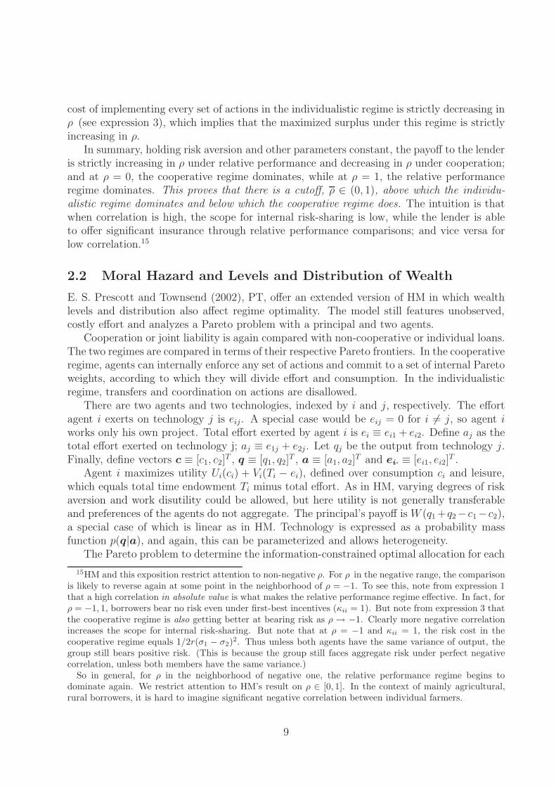
regime consists of maximizing a λ-weighted average of the borrowers’ utilities, subject to thelender’s expected utility reaching at least W and the appropriate incentive constraints. Sup-pose for simplicity that each of ci, qj , and eij can take on a finite number of values. In theindividualistic case, the credit contract induces individuals’ effort ei· and specifies individu-alized consumption amounts c as a function of output q.16 Linearity in compensation is notimposed however, and further, randomness in consumption is allowed. Even the contractitself can be randomized ex ante, inducing a random choice of effort. The more generalnotation is thus a lottery over all objects: Π(c, q, e1·, e2·). However, the optimal contractmay often involve non-random effort recommendations and consumption allocations.

The more general contract must satisfy probability measure constraints

Π(c, q, e1·, e2·) ≥ 0, ∀ c, q, e1·, e2·

and ∑c,q,e1·,e2·

Π(c, q, e1·, e2·) = 1.

The optimal contract is found by maximizing∑c,q,e1·,e2·

Π(c, q, e1·, e2·)∑

i

λi[Ui(ci) + Vi(Ti − ei)]

subject to: ∑c,q,e1·,e2·

Π(c, q, e1·, e2·)W (q1 + q2 − c1 − c2) ≥ W,

∑c

Π(c, q, e1·, e2·) = p(q|e1· + e2·)∑c,q

Π(c, q, e1·, e2·), ∀q, e1·, e2·,

and ∑c,q,e2·

Π(c, q, e1·,e2·)[U1(c1) + V1(T1 − e1)] ≥

∑c,q,e2·

Π(c, q, e1·, e2·)p(q|e1· + e2·)p(q|e1· + e2·)

[U1(c1) + V1(T1 − e1)], ∀e1·, e1·,

and an incentive constraint for agent 2 similar to the last inequality. The first constraintensures a given amount of resource extraction (possibly negative) from the pair. Note thatas W , the lender’s expected receipts, increases, in effect the wealth of the borrower decreases.The second ensures that the mechanism assigns technologically feasible probabilities, and thelast is an incentive constraint ensuring agent 1 abides by his recommended effort allocation.

In the cooperative, joint liability case, the borrowers are able to side contract. Thusthey can internally enforce any set of (Pareto optimal) actions, conditional on the borrowingcontract offered by the lender. They are also free to share risk internally by committing to expost transfers as in HM. This means that the contract cannot specify the ci’s separately, onlytotal group consumption, cg ≡ c1+c2. Similarly, it cannot specify the individual effort choices

16As in HM, loan size could be made to vary, but is regarded as fixed and dropped from the notation.

10

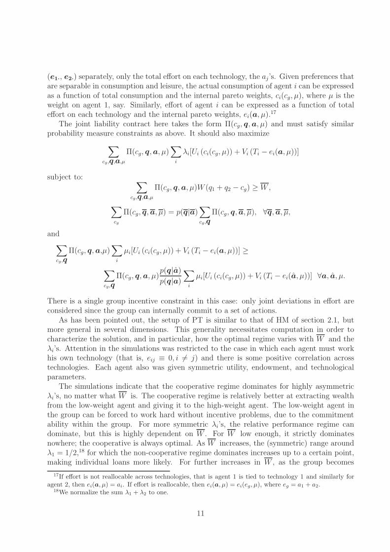
(e1·, e2·) separately, only the total effort on each technology, the aj’s. Given preferences thatare separable in consumption and leisure, the actual consumption of agent i can be expressedas a function of total consumption and the internal pareto weights, ci(cg, µ), where µ is theweight on agent 1, say. Similarly, effort of agent i can be expressed as a function of totaleffort on each technology and the internal pareto weights, ei(a, µ).17

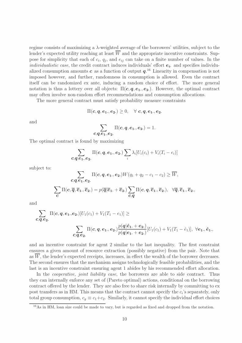
The joint liability contract here takes the form Π(cg, q, a, µ) and must satisfy similarprobability measure constraints as above. It should also maximize∑

cg,q,a,µ

Π(cg, q, a, µ)∑

i

λi[Ui (ci(cg, µ)) + Vi (Ti − ei(a, µ))]

subject to: ∑cg,q,a,µ

Π(cg, q, a, µ)W (q1 + q2 − cg) ≥ W,

∑cg

Π(cg, q, a, µ) = p(q|a)∑cg,q

Π(cg, q, a, µ), ∀q, a, µ,

and∑cg,q

Π(cg, q, a,µ)∑

i

µi[Ui (ci(cg, µ)) + Vi (Ti − ei(a, µ))] ≥

∑cg,q

Π(cg, q, a, µ)p(q|a)

p(q|a)

∑i

µi[Ui (ci(cg, µ)) + Vi (Ti − ei(a, µ))] ∀a, a, µ.

There is a single group incentive constraint in this case: only joint deviations in effort areconsidered since the group can internally commit to a set of actions.

As has been pointed out, the setup of PT is similar to that of HM of section 2.1, butmore general in several dimensions. This generality necessitates computation in order tocharacterize the solution, and in particular, how the optimal regime varies with W and theλi’s. Attention in the simulations was restricted to the case in which each agent must workhis own technology (that is, eij ≡ 0, i �= j) and there is some positive correlation acrosstechnologies. Each agent also was given symmetric utility, endowment, and technologicalparameters.

The simulations indicate that the cooperative regime dominates for highly asymmetricλi’s, no matter what W is. The cooperative regime is relatively better at extracting wealthfrom the low-weight agent and giving it to the high-weight agent. The low-weight agent inthe group can be forced to work hard without incentive problems, due to the commitmentability within the group. For more symmetric λi’s, the relative performance regime candominate, but this is highly dependent on W . For W low enough, it strictly dominatesnowhere; the cooperative is always optimal. As W increases, the (symmetric) range aroundλ1 = 1/2,18 for which the non-cooperative regime dominates increases up to a certain point,making individual loans more likely. For further increases in W , as the group becomes

17If effort is not reallocable across technologies, that is agent 1 is tied to technology 1 and similarly foragent 2, then ei(a, µ) = ai. If effort is reallocable, then ei(a, µ) = ei(eg, µ), where eg = a1 + a2.

18We normalize the sum λ1 + λ2 to one.

11

poorer, the (symmetric) range around λ1 = 1/2 for which the relative performance regimedominates diminishes, making the group regime attractive over a wider range.19

In a decentralization of this model, the payoff to the lender, W , would vary inversely withthe wealth of the borrowers, and the asymmetry of the λi’s would reflect wealth dispersionamong the borrowers. These simulations thus suggest that we should expect to see thecooperative regime occurring more frequently at higher levels of wealth inequality within agroup. Controlling for inequality, we should expect to see the cooperative regime varyingnegatively with wealth when wealth is low and positively when it is high. This is a U-shapedrelationship of the cooperative regime prevalence with group wealth.

2.3 Adverse Selection and Technological Correlation

Ghatak (1999) provides an adverse selection model of joint liability borrowing. Here theinternal information is on the risk-type. The key choices of the agent in this model arethe partner to join with in borrowing, and whether or not to borrow at all. Joint liabilityis shown to take advantage of the information borrowers have about each other in a waythat enables decreasing the interest rate and drawing in safer borrowers, thus mitigating theadverse selection problem.

Regarding the choice of the borrowing partner of the agent, Ghatak shows that agentsform groups that are homogeneous in risk-type. Regarding the choice about whether or notto borrow, the model delivers a cutoff risk-type, p, such that all borrowers more risky thanp borrow, and others do not. The latter prediction is our focus here.

A continuum of borrowers is assumed, each one with an exogenously given project indexedby a risk-type, p. This is the key heterogeneity. There is a density g(p) > 0 of borrowersat each type p ∈ [p, 1], where p is a parameter of the model. The project of a borrower oftype p yields output q(p) with probability p and gives zero output otherwise. Ghatak alsoassumes that

pq(p) = E, ∀p ∈ [p, 1].

Hence the borrowers do not differ in expected output. The only heterogeneity is in thesecond moment of this simple distribution, and one can verify that a lower p implies higherrisk, i.e. variance.

Borrowers are taken to be risk-neutral, unlike the previous models. It is assumed thatone unit each of capital and labor are required to carry out the project. Each potentialborrower is endowed with one unit of labor, which could be used by itself to produce u,and no capital. Capital is available from a lender who offers borrowers take-it-or-leave-itcontracts. Again, loan size could be introduced into the current notation, but as in the othermodels, we suppress it here.

19The intuition for the group regime’s wider range of dominance at high or low levels of W seems to be asfollows. For W low enough, the agents are not required to exert much effort. Both regimes are equally goodwhen providing incentives for effort is not critical and redistribution is unimportant. Thus both are equallygood at symmetric λi’s, whereas for asymmetric λi’s, the group regime dominates due to its advantage atredistributing wealth among the agents. For W high, the key is extracting wealth from the group. It appearsthe group regime is better at this because of internal commitment, while the relative performance regimerequires more high-powered incentives, i.e consumption rewards, to induce high effort. It is unclear howrobust this latter result is.

12

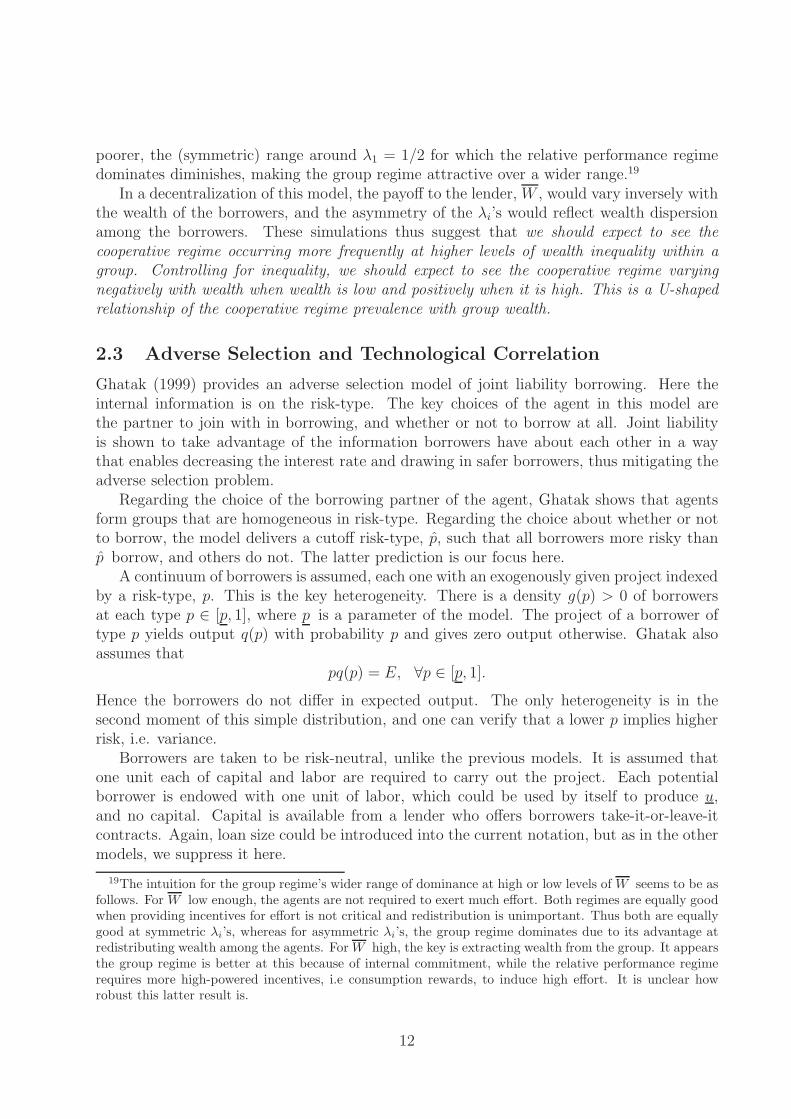
The lender is assumed to observe only whether each project has succeeded or failed; thusthe lender can contract on the binary outcome of success or failure, but not on the amountof output or risk-type, which would be optimal if these were observable.20 This implies that,in contrast to HM and PT, borrower payoff cannot depend on the borrowing pair’s outputother than through two binary functions, that is, depending only on whether each borrowerrealized returns greater than zero.

Ghatak focuses the analysis on groups of size two. A borrower of type p who pairs withone of type p′ has expected payoff of

E − pr − p(1 − p′)l,

where r > 0 is the interest rate and l > 0 the joint liability payment. The interest rate ispaid whenever the borrower succeeds and the joint liability payment whenever the borrowersucceeds and his partner does not. By inspection, the cross-partial of the payoff with respectto p and p′ is l > 0. This is sufficient to give that borrowers will match homogeneously inrisk-type, as Ghatak shows.21

Homogeneous matching means the payoff of a borrower of type p will be the following inequilibrium:

E − pr − p(1 − p)l.

Note that the derivative of the payoff with respect to p is −[r + l(1− 2p)]. As long as l ≤ r,which we assume, this derivative is strictly negative for p ∈ [p, 1). Thus, the safer an agent’stype, the lower his payoff from borrowing and undertaking the project. Since all agents havean outside option that pays u, agents will borrow if and only if the payoff from borrowingis greater than u. Given that the payoff of borrowing is declining in p, there exists a cutoffrisk-type, call it p, such that borrowers of type p > p will not find it optimal to borrow, andborrowers of type p < p will borrow.2223 This prediction of adverse selection in a limitedliability credit market is general and can be found in the literature at least as far back as

20Clearly, if type were observable, the lender could tailor the interest rate to each borrower’s likelihood ofsuccess and eliminate the adverse selection problem. If output q(p) were observable, this would be equivalentto knowing the borrower’s type in this model, since p = E/q(p) (and E would presumably be known if therewere many borrowers). This would then reduce to the case where type is observable and the lender canperfectly price discriminate.

The assumption of unobservable output in Ghatak distinguishes it from HM and PT, where the lenderdoes observe output. It is likely, however, that the same qualitative results could be obtained in Ghatak evenunder observable output, provided certain modifications to the output distributions were made, includingthat the support of the output distributions did not vary by type.

21Intuitively, safe borrowers benefit relatively more from safe partners. This is because safe borrowerssucceed more often, and are thus in the position of having a delinquent partner affect their payoff moreoften.

22This prediction is true ceteris paribus. If other characteristics, such as the outside option or expectedreturn, vary across the borrowers, then of course p varies also. We control for varying E and u usingobservable demographic, capital and occupational choice variables. Controlling for r is of less concern in ourdata, since BAAC national policy at the time of the survey dictated charging a fixed interest rate of 9% onloans under sixty thousand Thai baht; the group loan ceiling was below this.

23Ghatak provides conditions under which joint liability will completely eliminate adverse selection (sothat p = 1) and under which it will reduce but not eliminate the adverse selection problem (so that p < 1).Our test will only be valid for an interior cutoff (i.e. p < 1) and thus could in theory fail if joint liability haseliminated the adverse selection problem.

13

Theorem 1 in Stiglitz and Weiss (1981). Again, it should be noted that the adverse selectionhere is in the riskiness, not means, of project outcomes.

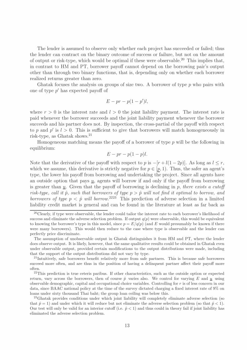
Next we modify the model beyond Ghatak’s work to consider correlation of output be-tween borrowers, in the spirit of HM. There is a unique way to introduce correlation thatpreserves the same individual probabilities of success, for a given pair of borrowers, (p, p′).It is displayed in the following table:

2 Succeeds (p′) 2 Fails (1 − p′)1 Succeeds (p) p p′ + ε p(1 − p′) − ε1 Fails (1 − p) (1 − p)p′ − ε (1 − p)(1 − p′) + ε

By inspection, each row and column adds to the correct individual probability of successor failure. Of course ε = 0 is the zero-correlation case, while ε > 0 introduces positivecorrelation.24 The above is the unique joint distribution, given a (p, p′) pair of individualprobabilities. However, there are many (p, p′) combinations, and each could in theory haveits own ε: ε(p, p′).

We consider two natural forms for the function ε(p, p′), both of which give some uniformityto the correlation structure across all project pairings. First we may assume ε(p, p′) to beconstant:25

ε(p, p′) = ε, ∀p, p′. (4)

The second assumption,26

ε(p, p′) = ρ ∗ min{p′(1 − p), p(1 − p′)}. (5)

gives any homogeneous group the same correlation coefficient over project returns, equal toρ, as a straightforward calculation shows. For non-homogeneous groups, that is those forwhom p �= p′, ρ is not the correlation coefficient, but something closely related: it is thecorrelation, expressed as a fraction of the maximum correlation possible given individualprobabilities of p and p′.27 When p = p′, the maximum possible correlation coefficient is one,so ρ equals the correlation coefficient. This formulation is arguably the most general, beingthe unique way of affecting each potential group’s (appropriately normalized) correlationcoefficient symmetrically.

24As does the HM analysis, we restrict attention here to positive correlation.25Note that ε is restricted in value by the need to keep each cell of the distribution matrix no less than

zero and no greater than one. For the off-diagonal cells of the matrix to be positive, we need ε to be lessthan p(1 − p′) and p′(1 − p). As p or p′ approaches one, ε is forced to zero, which is not interesting. Toavoid this problem, we can modify the support of risk-types innocuously to exclude those with probabilityof success near 1:

∃p ∈ (p, 1), such that ∀p ∈ (p, 1], g(p) = 0.

This assumption merely changes the support from [p, 1] to [p, p], ensuring that all borrowers face at leastsome uncertainty. One can verify that under this modified support, ε ≤ p(1 − p) is necessary (and sufficientif ε ≥ 0) to ensure no cell in the distribution matrix of every possible (p, p′) pairing exceeds one or falls belowzero.

26It is clear that under this second assumption, any ρ ∈ [0, 1] is allowable, that is, keeps each cell in thedistribution matrix of every possible (p, p′) pairing from exceeding one or falling below zero.

27Note that for non-homogeneous groups, it is a theoretical impossibility to have perfect correlation; twobinomial variables with different individual probabilities of success can never be perfectly correlated. Thefurther apart are the two probabilities, the lower the maximum correlation possible. One can calculate that

14

The first step in examining correlation is to determine how it affects the equilibriumhomogeneous matching result, if at all. The forms of correlation expressed in 4 and 5 donot, as can be shown by verifying that the gain to a risky borrower from switching to a safepartner is less than the loss to a safe borrower from switching to a risky partner (for ρ non-negative, see Ahlin and Townsend 2002). Given that homogeneous matching still obtains,the borrower payoff under correlation now becomes

E − pr − [p(1 − p) − ε(p, p)]l.

The indifference equation that defines the cutoff type p28 under assumption 4 becomes

E − pr − [p(1 − p) − ε]l = u, (6)

and under assumption 5,E − pr − p(1 − p)(1 − ρ)l = u. (7)

By inspection, the left-hand sides of equations 6 and 7 are increasing in ε and ρ, respectively.That is, higher correlation raises the payoff of the indifferent borrower. Clearly, for higherε, p will also have to be higher (since the borrowing payoff is still decreasing in p) in orderto bring down the payoff and keep it equal to u; the same is true for higher ρ.29 Sincep is higher, the mass of borrowers has increased, or in other words, the probability thatan agent chosen at random will borrow has increased. Thus, ceteris paribus, a populationamong whom technological correlation is higher will have more agents choose to borrow asgroup members and a higher chance that any given agent borrows in a group.

This result that correlation makes the group borrowing contract more likely is the oppo-site from HM. The idea here comes from the property of the model that a positive payoffonly occurs when the borrower is successful. Correlation shifts the weight in this state ofthe world toward the sub-state where the borrower’s partner is successful, away from thesub-state where the borrower’s partner fails. Thus it raises the payoff and draws in moreborrowers.30

the maximum correlation coefficient across two projects (p, p′), call it ρ(p, p′), is equal to

ρ(p, p′) = min{√

p(1 − p′)p′(1 − p)

,

√p′(1 − p)p(1 − p′)

}.

Further, the correlation coefficient corresponding to the ε(p, p′) of assumption 5 can be shown to equalρ ∗ ρ(p, p′). Thus ρ has the interpretation, described in the text, as the correlation expressed as a fractionof the maximum possible correlation, and it can vary freely from zero to one. Of course, it is clear from theformula that ρ(p, p) = 1, so for homogeneous groups, ρ is just the correlation coefficient itself.

28This is true for interior p.29In other words, total differentiation of equations 6 and 7, respectively, shows that dp/dε > 0 and

dp/dρ > 0.30Note that these comparisons involve a fixed interest rate r and liability payment l. If the lender perfectly

observed the degree of correlation, it might vary r and l with the level of correlation, and our comparisonswould not be valid. As noted earlier, however, BAAC national guidelines stipulated interest rates of 9%for loans under sixty thousand, which is above the group loan ceiling, so there is very little interest ratevariation (perhaps only noise) in the data. In general, the process seems best viewed as a standard contractbeing offered to any willing borrowers.

15

3 Empirical Results

3.1 Empirical Strategy

The predictions of HM and PT can be tested by relating the likelihood of the cooperative,group regime – vis a vis the relative performance, individual regime – to correlation andwealth distribution variables. In particular, HM predict the group regime to be less likelythe higher is correlation between agents’ output. PT predict the group regime to be morelikely the more disparate the wealth levels within the group, and the more extreme the wealthlevel of the group relative to the lender. In other words, there is a U-shaped relationship ofgroup wealth with the likelihood of the group regime.

To measure existence of the cooperative and relative performance regimes, we focus onborrowing contracts. The rural credit market is an a priori likely candidate for the existenceof moral hazard, due to lack of collateral of many poor borrowers and unobservability ofeffort. There is also significant risk to be borne in these predominantly agricultural settings.Thus the tradeoff between group and individual contracts analyzed in theory is likely to bepresent in our data.

In the theory, the key difference between the individual and group regimes is whetherthe agents can collude and enforce internal agreements. In practice this ability seems hardto measure, though it may be proxied well by variables measuring sharing and cooperativeactivities in other spheres of life (see Ahlin and Townsend 2002). The point of the theory,however, is that the contract itself may build in encouragement or facilitation of such co-operation, or leave it conspicuously absent. In other words, the theory relies on the lenderand/or borrowers being able to turn on or off the borrowers’ ability to side-contract. Itseems natural to interpret the formation of groups as such a facilitation of side-contracting.Groups have meetings together, are under a designated internal leader, and engage in signif-icant internal monitoring. In our data, the average borrowing group (from the BAAC) has70% of its members communicating with the group leader at least twice per week and 35%of its members at least six times per week.

Individual loans, on the other hand, can be thought of as the relative performance regime,though of course in reality the principal cannot enforce complete lack of cooperation betweenagents. He can, however, abstain from encouraging it. Further, the primary lender in ourdata, the BAAC, does seem to base its stringency toward one borrower in part on theperformance of other borrowers, as discussed in the introduction. It is at least reasonablethen to associate the relative performance regime in the theory with individual loans in thedata.

Tying these two regimes to individual and group loans, respectively, we face the difficultyof drawing the boundary lines of the group empirically. In the theory, contracts alwaysinvolve two agents. In practice, joint liability groups (of the BAAC) typically have betweenfive and fifteen members, a small minority having between fifteen and thirty. Further, we donot observe in our data the group with whom each borrowing household is matched. It iseven more difficult to determine the set of borrowers with whom an individual borrower isbeing compared in a relative performance regime; certainly there is no reason to expect thatthe comparison group contains just one other borrower, as in the theory. Our simplifyingassumption in both cases is that the village forms the boundary from which the group can

16

be drawn and among which comparisons are made for individual borrowers. The village isthe smallest unit into which our data classify each borrower. It makes sense as a boundaryfor explicit borrowing groups: in our data, over 65% of such groups (of the BAAC) have alltheir membership from a single village, and over 90% have more than half. Since correlationis likely higher within a village than across villages, it is probably also the best choice of arelative performance comparison group.31

To summarize, the data we use are household-level observations that show whether thehousehold is borrowing and under which regime, but do not allow us to determine explicitlygroup membership (whether the group is a comparison group under relative performance, oran explicit borrowing group under the cooperative regime). To measure32 wealth dispersionwithin the group, then, we use a measure of distance between the borrowing household’swealth and the village mean wealth. The assumption is that the further the household isaway from the village mean, the higher the likelihood that it is in a group with asymmetricwealth. We measure correlation within the group by the degree of clustering of superlativeyears (for household income) of this household with other households in the village. Again,the assumption is that the more this household’s good and bad years coincide with othersin the village, the more likely the case that it is in a group with high correlation. Finally, toproxy the wealth of the group, we use different combinations of the wealth of the householditself and the village average wealth of borrowing households. Each of these two componentshas its advantage. The wealth of the household itself is certainly a component of groupwealth, since we know for certain this household belongs to the borrowing group in question.However, the wealth of the remainder of the group is a more significant component of totalgroup wealth, since groups contain multiple households; but using the village average wealthof borrowers measures wealth of the remainder of the group with error.

Ultimately, we use these measures of group wealth, wealth dispersion, and correlation, allat the household level, to explain whether the household has a group loan. Since the theoryknows nothing of agents involved in both kinds of regimes or in neither, we exclude from theregression households with both kinds of loans or with neither. The results are detailed insection 3.3.

The Ghatak model focuses on risk-type and correlation as key determinants of whether ahousehold will borrow. We use the same household-level correlation measure described in thepreceding paragraphs, reflecting the coincidence of the household’s good and bad years withother households in the village. The risk-type measure applies the theory directly to sub-jective evaluations the household makes about the distribution its future income prospects.This measure is detailed in section 3.2.

The key decision, then, is what to do with households having individual loans, sincethe Ghatak theory does not leave room for them.33 One option is to exclude them, just

31One might argue under HM-type logic that forming cooperative groups out of borrowers from differentvillages would be optimal, since this would minimize correlation. However, the ability of such borrowers tomonitor and enforce internal agreements would presumably be low, due to geographic separation and lack ofcontact. Thus a group contract between borrowers from different villages may be ruled out as highly costlya priori.

32Variable construction is discussed in more detail in section 3.2.33The theory shows that joint liability contracts always produce more social surplus than individual liability

contracts, though they may not be Pareto optimal in that they can hurt the risky borrowers in equilibrium.

17

as households that did not fit into HM and PT theory were excluded in that specification.Another option is to include them and group them with households having group loans. Therationale for this would be that the key to the adverse selection result is not the form ofliability, individual or joint, but rather whether liability is limited.34 Thus if the individualloans are limited liability, they too should exhibit adverse selection. In fact it is likelythey are limited liability to some degree; as argued above, the collateral goes unseized notinfrequently and provisions are sometimes made. However, even in this case, it may be thatthese loans are significantly closer to full liability than are joint liability loans. This wouldargue for their inclusion with non-borrowing households in the regression, since full liabilitymakes risk-type unimportant. Further, the correlation result relies critically on both jointand limited liability, so this specification is clearly preferred on those grounds. Fortunately,the key results are insensitive to the differences in these specifications.

3.2 Description of Variables

Our data are taken from a detailed survey of households in Thailand conducted in 1997.The survey covers two contrasting regions in Thailand. The central region is relatively closeto Bangkok and enjoys a degree of industrialization as well as fertile land for farming. Thenortheast region is poorer and semi-arid. There is significant wealth variation both withinand across regions. Within regions, sampling was stratified based on ecological zones, toensure variation in good and bad years. This stratification affected choices of sub-counties,or tambons. Within tambons, choices of villages and of households within villages wererandom. In all 192 villages were surveyed. In virtually all of these villages, fifteen householdswere surveyed, giving a total sample size of 2875. Table I gives a summary of all dependentand independent variables used, reporting means for all but squared terms and standarddeviations for all but squared terms and dummy variables.

The dependent variables that we use are dummies reflecting whether the household hastaken out a group-guaranteed loan from a lending institution in the past year. There aretwo versions of this variable. The first, BAGPLOAN, restricts attention to group-guaranteedloans from the BAAC. This government institution is the primary institutional lender in ruralThailand: for example, 64% of institutional loans in our sample are from the BAAC. TheBAAC offers both individual loans, which much be guaranteed by some form of collateral,usually land, and joint liability loans. To receive the latter, one must form or join an officialBAAC-registered borrowing group and enter into a joint liability arrangement. BAGPLOANequals one if the household has had outstanding a loan from the BAAC in the past year andlists the collateral for this loan as either none, a single guarantor, or multiple guarantors.About 23% of the household sample has such a loan.

The second version of the dependent variable is GRUPLOAN, which incorporates group-guaranteed loans from the BAAC and other institutions. These others are typically smallerinstitutions such as agricultural cooperatives and often village-based ones such as produc-tion credit groups (PCGs), but they also include commercial banks.35 Using this broaderdefinition increases the proportion of the sample that qualifies as having a group-guaranteed

34Stiglitz and Weiss (1981) get the same result in the context of individual, limited liability.35Specifically, they include PCGs, commercial banks, agricultural cooperatives, village funds, rice banks,

as well as any other cooperatives, institutions, or programs that also lend funds.

18

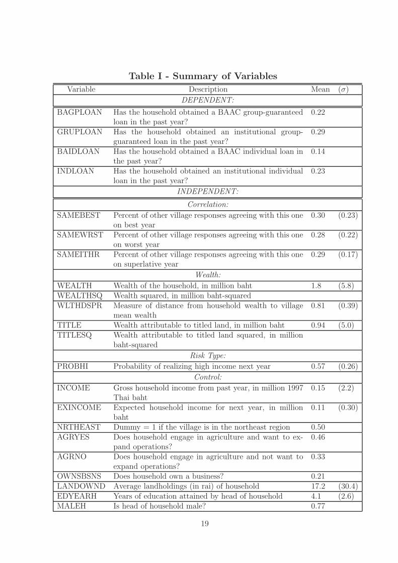
Table I - Summary of Variables

Variable Description Mean (σ)

DEPENDENT:

BAGPLOAN Has the household obtained a BAAC group-guaranteedloan in the past year?

0.22

GRUPLOAN Has the household obtained an institutional group-guaranteed loan in the past year?

0.29

BAIDLOAN Has the household obtained a BAAC individual loan inthe past year?

0.14

INDLOAN Has the household obtained an institutional individualloan in the past year?

0.23

INDEPENDENT:

Correlation:

SAMEBEST Percent of other village responses agreeing with this oneon best year

0.30 (0.23)

SAMEWRST Percent of other village responses agreeing with this oneon worst year

0.28 (0.22)

SAMEITHR Percent of other village responses agreeing with this oneon superlative year

0.29 (0.17)

Wealth:

WEALTH Wealth of the household, in million baht 1.8 (5.8)WEALTHSQ Wealth squared, in million baht-squaredWLTHDSPR Measure of distance from household wealth to village

mean wealth0.81 (0.39)

TITLE Wealth attributable to titled land, in million baht 0.94 (5.0)TITLESQ Wealth attributable to titled land squared, in million

baht-squared

Risk Type:

PROBHI Probability of realizing high income next year 0.57 (0.26)

Control:

INCOME Gross household income from past year, in million 1997Thai baht

0.15 (2.2)

EXINCOME Expected household income for next year, in millionbaht

0.11 (0.30)

NRTHEAST Dummy = 1 if the village is in the northeast region 0.50AGRYES Does household engage in agriculture and want to ex-

pand operations?0.46

AGRNO Does household engage in agriculture and not want toexpand operations?

0.33

OWNSBSNS Does household own a business? 0.21LANDOWND Average landholdings (in rai) of household 17.2 (30.4)EDYEARH Years of education attained by head of household 4.1 (2.6)MALEH Is head of household male? 0.77

19

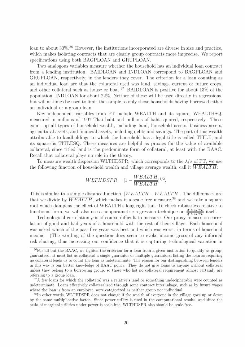
loan to about 30%.36 However, the institutions incorporated are diverse in size and practice,which makes isolating contracts that are clearly group contracts more imprecise. We reportspecifications using both BAGPLOAN and GRUPLOAN.

Two analogous variables measure whether the household has an individual loan contractfrom a lending institution. BAIDLOAN and INDLOAN correspond to BAGPLOAN andGRUPLOAN, respectively, in the lenders they cover. The criterion for a loan counting asan individual loan are that the collateral used was land, savings, current or future crops,and other collateral such as house or boat.37 BAIDLOAN is positive for about 13% of thepopulation, INDLOAN for about 22%. Neither of these will be used directly in regressions,but will at times be used to limit the sample to only those households having borrowed eitheran individual or a group loan.

Key independent variables from PT include WEALTH and its square, WEALTHSQ,measured in millions of 1997 Thai baht and millions of baht-squared, respectively. Thesecount up all types of household wealth, including land, household assets, business assets,agricultural assets, and financial assets, including debts and savings. The part of this wealthattributable to landholdings to which the household has a legal title is called TITLE, andits square is TITLESQ. These measures are helpful as proxies for the value of availablecollateral, since titled land is the predominate form of collateral, at least with the BAAC.Recall that collateral plays no role in the theory.

To measure wealth dispersion WLTHDSPR, which corresponds to the λi’s of PT, we usethe following function of household wealth and village average wealth, call it WEALTH:

WLTHDSPR = |1 − WEALTH

WEALTH|1/2.

This is similar to a simple distance function, |WEALTH −WEALTH|. The differences arethat we divide by WEALTH, which makes it a scale-free measure,38 and we take a squareroot which dampens the effect of WEALTH’s long right tail. To check robustness relative tofunctional form, we will also use a nonparametric regression technique on WEALTH

WEALTHitself.

Technological correlation ρ is of course difficult to measure. Our proxy focuses on corre-lation of good and bad years of a household with the rest of their village. Each householdwas asked which of the past five years was best and which was worst, in terms of householdincome. (The wording of the question does seem to evoke income gross of any informalrisk sharing, thus increasing our confidence that it is capturing technological variation in

36For all but the BAAC, we tighten the criterion for a loan from a given institution to qualify as group-guaranteed. It must list as collateral a single guarantor or multiple guarantors; listing the loan as requiringno collateral leads us to count the loan as indeterminate. The reason for our distinguishing between lendersin this way is our better knowledge of BAAC policy. They do not give loans to anyone without collateralunless they belong to a borrowing group, so those who list no collateral requirement almost certainly arereferring to a group loan.

37A few loans for which the collateral was a relative’s land or something undecipherable were counted asindeterminate. Loans effectively collateralized through some contract interlinkage, such as by future wageswhere the loan is from an employer, were categorized as neither group nor individual.

38In other words, WLTHDSPR does not change if the wealth of everyone in the village goes up or downby the same multiplicative factor. Since power utility is used in the computational results, and since theratio of marginal utilities under power is scale-free, WLTHDSPR also should be scale-free.

20

income.) SAMEBEST, SAMEWRST, and SAMEITHR, reflect the percent of the other vil-lage households’ responses that coincide with this household’s responses regarding the bestyear, worst year, and about either year, respectively.39 We use each of these measures. Thetheories we test do not give clear direction on which should be more helpful.

The final key variable to measure is the risk-type of the borrower. We do so usingsubjective income assessments, taking the Ghatak model quite literally. Specifically, eachhousehold was asked what their income would be in the coming year if it were a good year(Hi), what their income would be if it were a bad year (Lo), and what they expected theirincome to be (Ex). We assume the income distribution is binomial over the high and lowstates, as in the Ghatak model. The probability of success, PROBHI, is then calculated tobe

PROBHI =Ex − Lo

Hi − Lo,

using the fact that PROBHI ∗ Hi + (1 − PROBHI) ∗ Lo = Ex.Several control variables are included, suggested by theory, institutional details, or practi-

cality. We include next year’s expected income (Ex), called EXINCOME, in our regressions.This is necessary because the Ghatak model assumes expected returns to be the same acrossall borrowers, while it of course varies in our data. We also include a comprehensive measureof income over the past twelve months, INCOME.40

The household head’s gender and years of education are controlled for in MALEH (malecoded as one) and EDYEARH, respectively. We also include a dummy variable, NRTHEAST,equaling one for the 50% of households in the poorer Northeast region. These are alsoimportant controls because the Ghatak model assumes the same outside (non-borrowing)option u for all borrowers, while outside options clearly vary in our data.

Finally, we control for eligibility and desire for a loan. Households were asked whetheror not they engage in agricultural activity, and if so, whether or not they would like toexpand their operations. From these questions we derive two dummy variables, AGRYESand AGRNO. AGRYES (AGRNO) equals one for the 46% (33%) of households that engagein agricultural activity and would (would not) like to expand their activity. The remaining21% of households for whom neither equals one are those who do not engage in agriculturalactivity. It is crucial to control for occupation, since the BAAC and several other institutionallenders targeted agricultural workers exclusively at the time of the survey. One further proxyfor desirability of a loan is the dummy variable OWNSBSNS, which equals one for the 21%of households that own a business.41

3.3 Logit Results

We use simple logits since the dependent variables, whether the household has a grouploan, are dummies. We report twelve specifications, varying across the three measures of

39For example, if a household lists the same best year as 4 of 12 other village households and the sameworst year as 7 of 14 other village respondents, then SAMEBEST = 4/12, SAMEWRST = 7/14, andSAMEITHR = 11/26. (Some households answer one question but not the other.)

40In some footnoted specifications we also control for the variance of next year’s income, using the subjec-tive income assessments described in the preceding paragraphs.

41It is purely coincidental that the same percent of households own businesses and do not engage inagriculture: there are households of whom both are true, and of whom neither are true.

21

correlation, the two versions of the dependent variable, and the sample chosen, whetherrestricted or unrestricted. More specifically, the restricted sample includes only those house-holds that have either a group-guaranteed BAAC (or institutional) loan, or an individualBAAC (or institutional) loan. That is, it includes only households for whom BAGPLOAN+BAIDLOAN = 1 (or GRUPLOAN + INDLOAN = 1). The rationale for examining thisrestricted sample is that HM and PT focus on the choice between cooperative and relativeperformance regimes given that one must be chosen. Thus the restricted sample regressions,though smaller in amount of data, are arguably more appropriate tests of HM and PT.

The logit results are reported in tables II and III, for the restricted and entire samples,respectively. It should also be noted that in each regression, we exclude households whohave not answered the questions about both best and worst years or whose village does notcontain at least four responses to each of these questions.42

Table II is the preferred specification for testing HM and PT. In all specifications, wealthlevels exhibit a U-shaped relationship with the group contract. These coefficients are allsignificant at the 5% significance level, except that under BCGPLOAN the coefficient onWEALTHSQ drops to the 10% significance level and under GRUPLOAN the coefficient onWEALTH drops to the 10% level. These baseline specifications give strong evidence for thewealth level predictions of PT.

The trough of the U-shaped relationship is around 6.4 million baht for BAGPLOAN and8.4 million baht for GRUPLOAN. This leaves 5-6% of the sample on the upward slopingsegment of the relationship. The U-shape remains significant under exclusion of householdswith wealth greater than 20 million (1.4% of the data).43 We check a cubic relationshipfor robustness and find a very similar picture: coefficients on WEALTH and WEALTHSQof the same sign as in Table II and significant at 1%, and the coefficient on WEALTHCBnegative and significant at 5% or 10% depending on specification. Further, the relationshipis declining to a trough between 5 and 6 million baht, then increasing to a peak at just over21 million, and declining from there (for just over 1% of the data). Thus the U-shape overvirtually all the data appears robust.

The same relationship is estimated using Yatchew’s (1998) estimator.44 The results usingboth dependent variables (and SAMEITHR as the measure of correlation) are pictured in

42SAMEITHR is valid in about 66% of households, after dropping households from villages where lessthan eight total responses to the two questions exist. SAMEBEST is valid in about 71% of households andSAMEWRST in about 80% of households, after dropping households from villages where less than four totalresponses to the respective question exist. For the regressions we report, we restrict each specification to the66% of households that have valid information for both SAMEBEST and SAMEWRST. This ensures thesample is not changing as we use different measures of correlation. We have run the regressions using all thedata available in each specification, and the results become somewhat different, but not enough to changeour qualitative conclusions.

43It does disappear as this cutoff decreases to 10 million (3.4% of the data); but this is not surprising sincewe are ignoring a significant fraction of households above the turning point.

44Specifically, a partially linear model is assumed where all the regressors but wealth affect the dependentvariable linearly, while wealth can have any kind of smooth effect. Fifth-order optimal differencing is usedto remove the effect of wealth and estimate the linear coefficients. The effect of all the variables but wealthis then substracted from the dependent variable to form a residual. Residuals are then demeaned, since weare not concerned with the intercept, and are put as the dependent variable in a locally linear regressionwith wealth as the predictor. We use a bandwidth to incorporate 80% of the data and the tri-cube weightingfunction (see Cleveland 1979 and Fan 1992) to downweight observations wg, say, further from the current

22

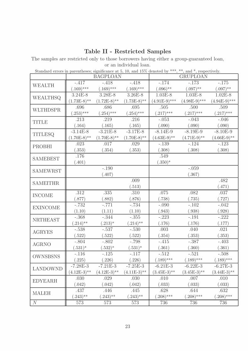
Table II - Restricted SamplesThe samples are restricted only to those borrowers having either a group-guaranteed loan,

or an individual loan.Standard errors in parentheses; significance at 5, 10, and 15% denoted by ***, **, and *, respectively.

BAGPLOAN GRUPLOAN-.417 -.418 -.418 -.174 -.173 -.175

WEALTH(.169)*** (.169)*** (.169)*** (.096)** (.097)** (.097)**3.24E-8 3.28E-8 3.26E-8 1.03E-8 1.03E-8 1.02E-8

WEALTHSQ(1.73E-8)** (1.72E-8)** (1.73E-8)** (4.91E-9)*** (4.98E-9)*** (4.94E-9)***

.696 .686 .695 .505 .500 .509WLTHDSPR

(.253)*** (.254)*** (.254)*** (.217)*** (.217)*** (.217)***.213 .219 .216 -.053 -.043 -.046

TITLE(.164) (.165) (.165) (.090) (.090) (.090)

-3.14E-8 -3.21E-8 -3.17E-8 -8.14E-9 -8.19E-9 -8.10E-9TITLESQ

(1.70E-8)** (1.70E-8)** (1.70E-8)** (4.63E-9)** (4.71E-9)** (4.66E-9)**.023 .017 .029 -.139 -.124 -.123

PROBHI(.353) (.354) (.353) (.308) (.308) (.308).176 .549

SAMEBEST(.401) (.350)*

-.190 -.059SAMEWRST

(.407) (.367).009 .482

SAMEITHR(.513) (.471)

.312 .335 .310 .075 .082 .037INCOME

(.877) (.882) (.876) (.738) (.735) (.727)-.732 -.771 -.734 -.090 -.102 -.042

EXINCOME(1.10) (1.11) (1.10) (.943) (.938) (.928)-.368 -.344 -.355 -.223 -.191 -.222

NRTHEAST(.214)** (.213)* (.214)** (.176) (.176) (.177)-.538 -.537 -.530 .003 .040 .021

AGRYES(.522) (.522) (.522) (.354) (.353) (.353)-.804 -.802 -.798 -.415 -.387 -.403

AGRNO(.531)* (.532)* (.531)* (.361) (.360) (.361)-.116 -.125 -.117 -.512 -.521 -.508

OWNSBSNS(.225) (.226) (.226) (.189)*** (.189)*** (.189)***

-7.28E-3 -7.21E-3 -7.25E-3 -6.21E-3 -6.22E-3 -6.27E-3LANDOWND

(4.12E-3)** (4.12E-3)** (4.11E-3)** (3.45E-3)** (3.45E-3)** (3.44E-3)**.030 .029 .030 .010 .007 .010

EDYEARH(.042) (.042) (.042) (.033) (.033) (.033).437 .446 .445 .628 .644 .632

MALEH(.243)** (.243)** (.243)** (.208)*** (.208)*** (.208)***

N 573 573 573 736 736 736

23

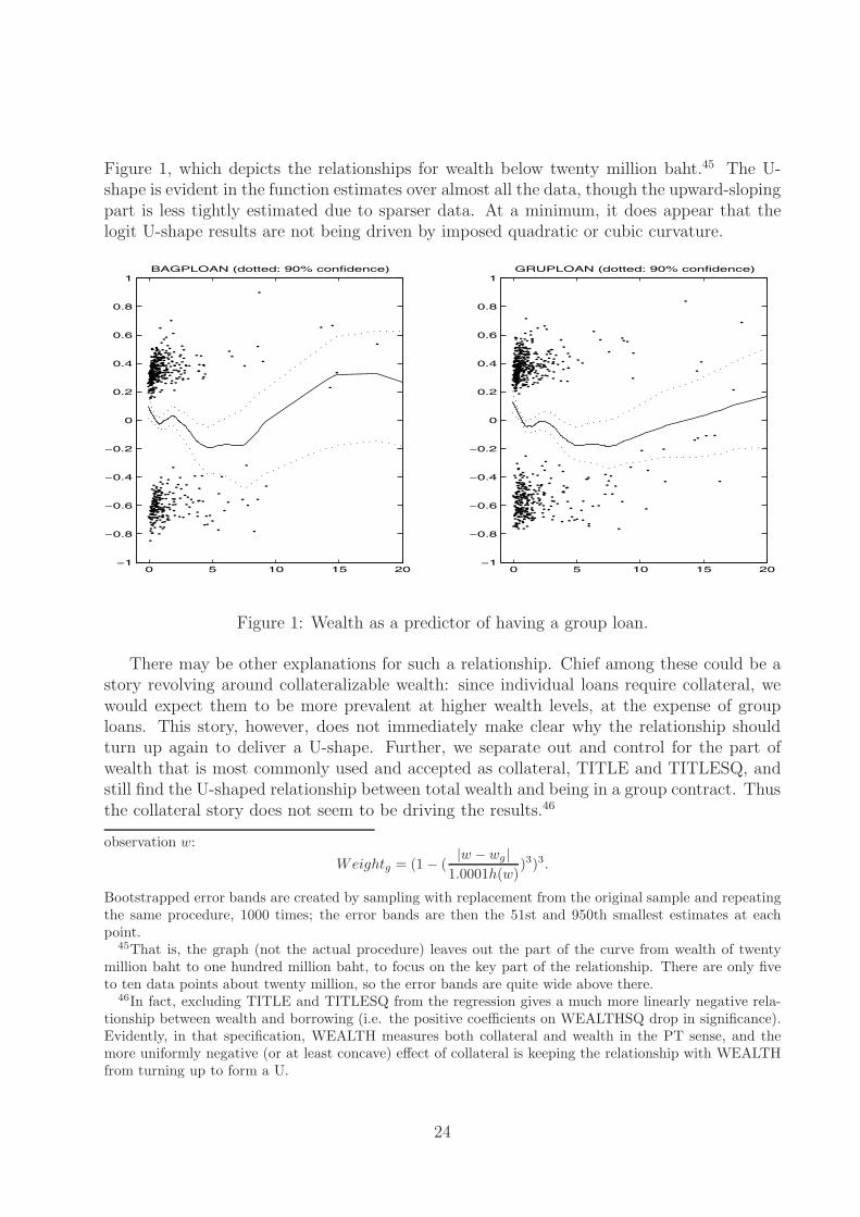
Figure 1, which depicts the relationships for wealth below twenty million baht.45 The U-shape is evident in the function estimates over almost all the data, though the upward-slopingpart is less tightly estimated due to sparser data. At a minimum, it does appear that thelogit U-shape results are not being driven by imposed quadratic or cubic curvature.

0 5 10 15 20−1

−0.8

−0.6

−0.4

−0.2

0

0.2

0.4

0.6

0.8

1BAGPLOAN (dotted: 90% confidence)

0 5 10 15 20−1

−0.8

−0.6

−0.4

−0.2

0

0.2

0.4

0.6

0.8

1GRUPLOAN (dotted: 90% confidence)

Figure 1: Wealth as a predictor of having a group loan.

There may be other explanations for such a relationship. Chief among these could be astory revolving around collateralizable wealth: since individual loans require collateral, wewould expect them to be more prevalent at higher wealth levels, at the expense of grouploans. This story, however, does not immediately make clear why the relationship shouldturn up again to deliver a U-shape. Further, we separate out and control for the part ofwealth that is most commonly used and accepted as collateral, TITLE and TITLESQ, andstill find the U-shaped relationship between total wealth and being in a group contract. Thusthe collateral story does not seem to be driving the results.46

observation w:

Weightg = (1 − (|w − wg|

1.0001h(w))3)3.

Bootstrapped error bands are created by sampling with replacement from the original sample and repeatingthe same procedure, 1000 times; the error bands are then the 51st and 950th smallest estimates at eachpoint.

45That is, the graph (not the actual procedure) leaves out the part of the curve from wealth of twentymillion baht to one hundred million baht, to focus on the key part of the relationship. There are only fiveto ten data points about twenty million, so the error bands are quite wide above there.

46In fact, excluding TITLE and TITLESQ from the regression gives a much more linearly negative rela-tionship between wealth and borrowing (i.e. the positive coefficients on WEALTHSQ drop in significance).Evidently, in that specification, WEALTH measures both collateral and wealth in the PT sense, and themore uniformly negative (or at least concave) effect of collateral is keeping the relationship with WEALTHfrom turning up to form a U.

24

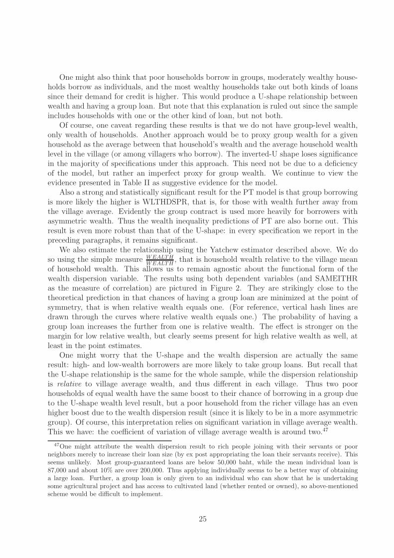
One might also think that poor households borrow in groups, moderately wealthy house-holds borrow as individuals, and the most wealthy households take out both kinds of loanssince their demand for credit is higher. This would produce a U-shape relationship betweenwealth and having a group loan. But note that this explanation is ruled out since the sampleincludes households with one or the other kind of loan, but not both.

Of course, one caveat regarding these results is that we do not have group-level wealth,only wealth of households. Another approach would be to proxy group wealth for a givenhousehold as the average between that household’s wealth and the average household wealthlevel in the village (or among villagers who borrow). The inverted-U shape loses significancein the majority of specifications under this approach. This need not be due to a deficiencyof the model, but rather an imperfect proxy for group wealth. We continue to view theevidence presented in Table II as suggestive evidence for the model.

Also a strong and statistically significant result for the PT model is that group borrowingis more likely the higher is WLTHDSPR, that is, for those with wealth further away fromthe village average. Evidently the group contract is used more heavily for borrowers withasymmetric wealth. Thus the wealth inequality predictions of PT are also borne out. Thisresult is even more robust than that of the U-shape: in every specification we report in thepreceding paragraphs, it remains significant.

We also estimate the relationship using the Yatchew estimator described above. We doso using the simple measure WEALTH

WEALTH, that is household wealth relative to the village mean

of household wealth. This allows us to remain agnostic about the functional form of thewealth dispersion variable. The results using both dependent variables (and SAMEITHRas the measure of correlation) are pictured in Figure 2. They are strikingly close to thetheoretical prediction in that chances of having a group loan are minimized at the point ofsymmetry, that is when relative wealth equals one. (For reference, vertical hash lines aredrawn through the curves where relative wealth equals one.) The probability of having agroup loan increases the further from one is relative wealth. The effect is stronger on themargin for low relative wealth, but clearly seems present for high relative wealth as well, atleast in the point estimates.

One might worry that the U-shape and the wealth dispersion are actually the sameresult: high- and low-wealth borrowers are more likely to take group loans. But recall thatthe U-shape relationship is the same for the whole sample, while the dispersion relationshipis relative to village average wealth, and thus different in each village. Thus two poorhouseholds of equal wealth have the same boost to their chance of borrowing in a group dueto the U-shape wealth level result, but a poor household from the richer village has an evenhigher boost due to the wealth dispersion result (since it is likely to be in a more asymmetricgroup). Of course, this interpretation relies on significant variation in village average wealth.This we have: the coefficient of variation of village average wealth is around two.47

47One might attribute the wealth dispersion result to rich people joining with their servants or poorneighbors merely to increase their loan size (by ex post appropriating the loan their servants receive). Thisseems unlikely. Most group-guaranteed loans are below 50,000 baht, while the mean individual loan is87,000 and about 10% are over 200,000. Thus applying individually seems to be a better way of obtaininga large loan. Further, a group loan is only given to an individual who can show that he is undertakingsome agricultural project and has access to cultivated land (whether rented or owned), so above-mentionedscheme would be difficult to implement.

25

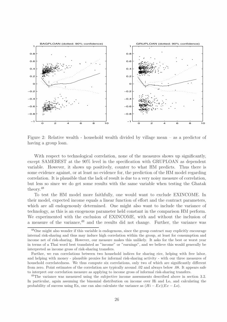
0 2 4 6 8 10−1

−0.8

−0.6

−0.4

−0.2

0

0.2

0.4

0.6

0.8

1BAGPLOAN (dotted: 90% confidence)

0 2 4 6 8 10−1

−0.8

−0.6

−0.4

−0.2

0

0.2

0.4

0.6

0.8

1GRUPLOAN (dotted: 90% confidence)

Figure 2: Relative wealth - household wealth divided by village mean – as a predictor ofhaving a group loan.

With respect to technological correlation, none of the measures shows up significantly,except SAMEBEST at the 90% level in the specification with GRUPLOAN as dependentvariable. However, it shows up positively, counter to what HM predicts. Thus there issome evidence against, or at least no evidence for, the prediction of the HM model regardingcorrelation. It is plausible that the lack of result is due to a very noisy measure of correlation,but less so since we do get some results with the same variable when testing the Ghataktheory.48

To test the HM model more faithfully, one would want to exclude EXINCOME. Intheir model, expected income equals a linear function of effort and the contract parameters,which are all endogenously determined. One might also want to include the variance oftechnology, as this is an exogenous parameter held constant in the comparison HM perform.We experimented with the exclusion of EXINCOME, with and without the inclusion ofa measure of the variance,49 and the results did not change. Further, the variance was

48One might also wonder if this variable is endogenous, since the group contract may explicitly encourageinternal risk-sharing and thus may induce high correlation within the group, at least for consumption andincome net of risk-sharing. However, our measure makes this unlikely. It asks for the best or worst yearin terms of a Thai word best translated as ”income” or ”earnings”, and we believe this would generally beinterpreted as income gross of risk-sharing transfers.

Further, we run correlations between two household indices for sharing rice, helping with free labor,and helping with money - plausible proxies for informal risk-sharing activity - with our three measures ofhousehold correlatedness. We thus compute six correlations, only two of which are significantly differentfrom zero. Point estimates of the correlation are typically around .02 and always below .08. It appears safeto interpret our correlation measure as applying to income gross of informal risk-sharing transfers.

49The variance was measured using the subjective income assessments described above in section 3.2.In particular, again assuming the binomial distribution on income over Hi and Lo, and calculating theprobability of success using Ex, one can also calculate the variance as (Hi − Ex)(Ex − Lo).

26

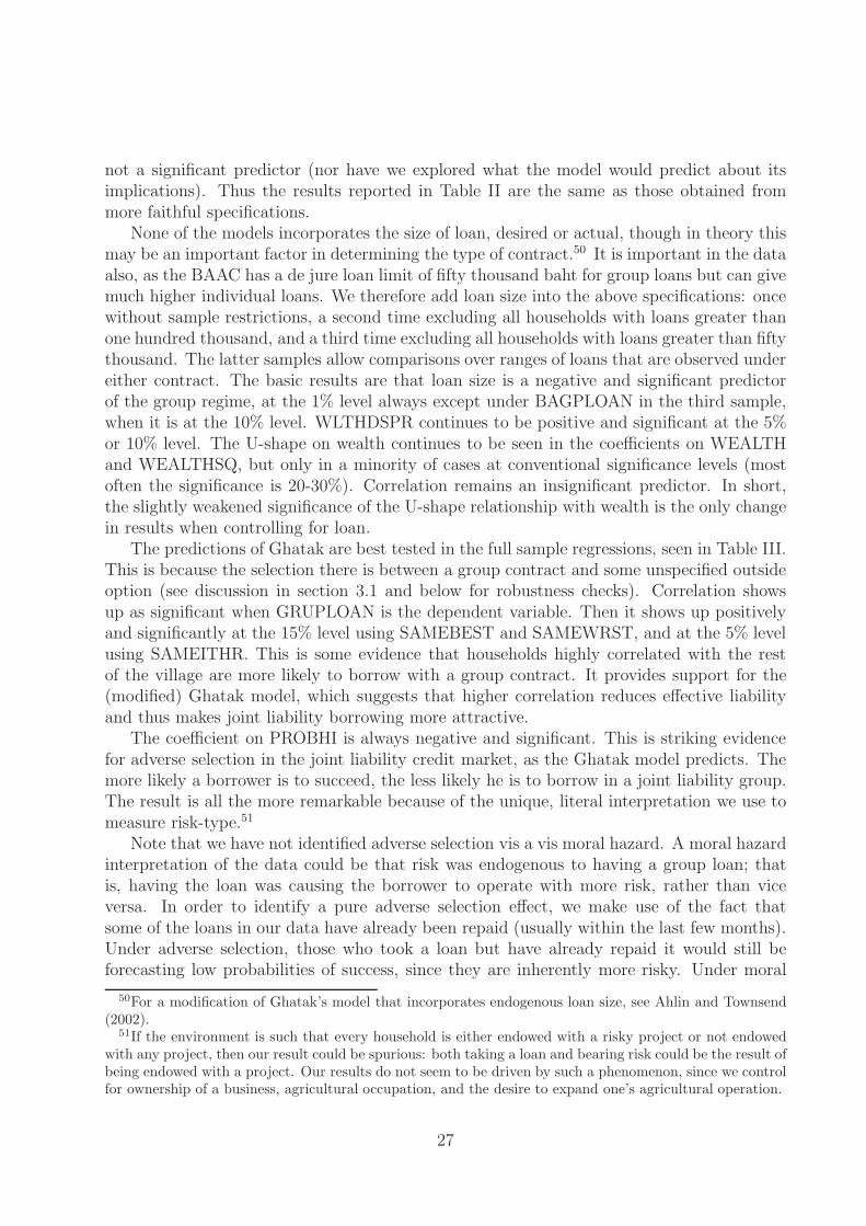
not a significant predictor (nor have we explored what the model would predict about itsimplications). Thus the results reported in Table II are the same as those obtained frommore faithful specifications.

None of the models incorporates the size of loan, desired or actual, though in theory thismay be an important factor in determining the type of contract.50 It is important in the dataalso, as the BAAC has a de jure loan limit of fifty thousand baht for group loans but can givemuch higher individual loans. We therefore add loan size into the above specifications: oncewithout sample restrictions, a second time excluding all households with loans greater thanone hundred thousand, and a third time excluding all households with loans greater than fiftythousand. The latter samples allow comparisons over ranges of loans that are observed undereither contract. The basic results are that loan size is a negative and significant predictorof the group regime, at the 1% level always except under BAGPLOAN in the third sample,when it is at the 10% level. WLTHDSPR continues to be positive and significant at the 5%or 10% level. The U-shape on wealth continues to be seen in the coefficients on WEALTHand WEALTHSQ, but only in a minority of cases at conventional significance levels (mostoften the significance is 20-30%). Correlation remains an insignificant predictor. In short,the slightly weakened significance of the U-shape relationship with wealth is the only changein results when controlling for loan.

The predictions of Ghatak are best tested in the full sample regressions, seen in Table III.This is because the selection there is between a group contract and some unspecified outsideoption (see discussion in section 3.1 and below for robustness checks). Correlation showsup as significant when GRUPLOAN is the dependent variable. Then it shows up positivelyand significantly at the 15% level using SAMEBEST and SAMEWRST, and at the 5% levelusing SAMEITHR. This is some evidence that households highly correlated with the restof the village are more likely to borrow with a group contract. It provides support for the(modified) Ghatak model, which suggests that higher correlation reduces effective liabilityand thus makes joint liability borrowing more attractive.

The coefficient on PROBHI is always negative and significant. This is striking evidencefor adverse selection in the joint liability credit market, as the Ghatak model predicts. Themore likely a borrower is to succeed, the less likely he is to borrow in a joint liability group.The result is all the more remarkable because of the unique, literal interpretation we use tomeasure risk-type.51

Note that we have not identified adverse selection vis a vis moral hazard. A moral hazardinterpretation of the data could be that risk was endogenous to having a group loan; thatis, having the loan was causing the borrower to operate with more risk, rather than viceversa. In order to identify a pure adverse selection effect, we make use of the fact thatsome of the loans in our data have already been repaid (usually within the last few months).Under adverse selection, those who took a loan but have already repaid it would still beforecasting low probabilities of success, since they are inherently more risky. Under moral

50For a modification of Ghatak’s model that incorporates endogenous loan size, see Ahlin and Townsend(2002).

51If the environment is such that every household is either endowed with a risky project or not endowedwith any project, then our result could be spurious: both taking a loan and bearing risk could be the result ofbeing endowed with a project. Our results do not seem to be driven by such a phenomenon, since we controlfor ownership of a business, agricultural occupation, and the desire to expand one’s agricultural operation.

27

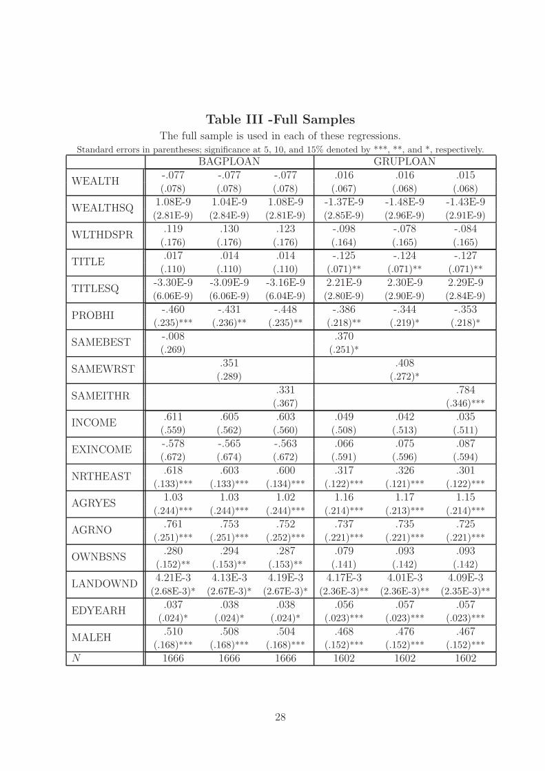
Table III -Full SamplesThe full sample is used in each of these regressions.

Standard errors in parentheses; significance at 5, 10, and 15% denoted by ***, **, and *, respectively.BAGPLOAN GRUPLOAN

-.077 -.077 -.077 .016 .016 .015WEALTH

(.078) (.078) (.078) (.067) (.068) (.068)1.08E-9 1.04E-9 1.08E-9 -1.37E-9 -1.48E-9 -1.43E-9

WEALTHSQ(2.81E-9) (2.84E-9) (2.81E-9) (2.85E-9) (2.96E-9) (2.91E-9)

.119 .130 .123 -.098 -.078 -.084WLTHDSPR

(.176) (.176) (.176) (.164) (.165) (.165).017 .014 .014 -.125 -.124 -.127

TITLE(.110) (.110) (.110) (.071)** (.071)** (.071)**

-3.30E-9 -3.09E-9 -3.16E-9 2.21E-9 2.30E-9 2.29E-9TITLESQ

(6.06E-9) (6.06E-9) (6.04E-9) (2.80E-9) (2.90E-9) (2.84E-9)-.460 -.431 -.448 -.386 -.344 -.353

PROBHI(.235)*** (.236)** (.235)** (.218)** (.219)* (.218)*

-.008 .370SAMEBEST

(.269) (.251)*.351 .408

SAMEWRST(.289) (.272)*

.331 .784SAMEITHR

(.367) (.346)***.611 .605 .603 .049 .042 .035

INCOME(.559) (.562) (.560) (.508) (.513) (.511)-.578 -.565 -.563 .066 .075 .087

EXINCOME(.672) (.674) (.672) (.591) (.596) (.594).618 .603 .600 .317 .326 .301

NRTHEAST(.133)*** (.133)*** (.134)*** (.122)*** (.121)*** (.122)***

1.03 1.03 1.02 1.16 1.17 1.15AGRYES

(.244)*** (.244)*** (.244)*** (.214)*** (.213)*** (.214)***.761 .753 .752 .737 .735 .725

AGRNO(.251)*** (.251)*** (.252)*** (.221)*** (.221)*** (.221)***

.280 .294 .287 .079 .093 .093OWNBSNS

(.152)** (.153)** (.153)** (.141) (.142) (.142)4.21E-3 4.13E-3 4.19E-3 4.17E-3 4.01E-3 4.09E-3

LANDOWND(2.68E-3)* (2.67E-3)* (2.67E-3)* (2.36E-3)** (2.36E-3)** (2.35E-3)**

.037 .038 .038 .056 .057 .057EDYEARH

(.024)* (.024)* (.024)* (.023)*** (.023)*** (.023)***.510 .508 .504 .468 .476 .467

MALEH(.168)*** (.168)*** (.168)*** (.152)*** (.152)*** (.152)***

N 1666 1666 1666 1602 1602 1602

28

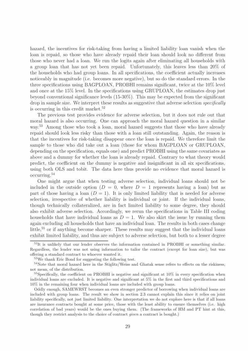
hazard, the incentives for risk-taking from having a limited liability loan vanish when theloan is repaid, so those who have already repaid their loan should look no different fromthose who never had a loan. We run the logits again after eliminating all households witha group loan that has not yet been repaid. Unfortunately, this leaves less than 20% ofthe households who had group loans. In all specifications, the coefficient actually increasesnoticeably in magnitude (i.e. becomes more negative), but so do the standard errors. In thethree specifications using BAGPLOAN, PROBHI remains significant, twice at the 10% leveland once at the 15% level. In the specifications using GRUPLOAN, the estimates drop justbeyond conventional significance levels (15-30%). This may be expected from the significantdrop in sample size. We interpret these results as suggestive that adverse selection specificallyis occurring in this credit market.52

The previous test provides evidence for adverse selection, but it does not rule out thatmoral hazard is also occurring. One can approach the moral hazard question in a similarway.53 Among those who took a loan, moral hazard suggests that those who have alreadyrepaid should look less risky than those with a loan still outstanding. Again, the reason isthat the incentives for risk-taking disappear once the loan is repaid. We therefore limit thesample to those who did take out a loan (those for whom BAGPLOAN or GRUPLOAN,depending on the specification, equals one) and predict PROBHI using the same covariates asabove and a dummy for whether the loan is already repaid. Contrary to what theory wouldpredict, the coefficient on the dummy is negative and insignificant in all six specifications,using both OLS and tobit. The data here thus provide no evidence that moral hazard isoccurring.54

One might argue that when testing adverse selection, individual loans should not beincluded in the outside option (D = 0, where D = 1 represents having a loan) but aspart of those having a loan (D = 1). It is only limited liability that is needed for adverseselection, irrespective of whether liability is individual or joint. If the individual loans,though technically collateralized, are in fact limited liability to some degree, they shouldalso exhibit adverse selection. Accordingly, we rerun the specifications in Table III codinghouseholds that have individual loans as D = 1. We also skirt the issue by running themagain excluding all households that have an individual loan. The results in both cases changelittle,55 or if anything become sharper. These results may suggest that the individual loansexhibit limited liability, and thus are subject to adverse selection, but both to a lesser degree

52It is unlikely that our lender observes the information contained in PROBHI or something similar.Regardless, the lender was not using information to tailor the contract (except for loan size), but wasoffering a standard contract to whoever wanted it.

53We thank Eric Bond for suggesting the following test.54Note that moral hazard here in the Stiglitz/Weiss and Ghatak sense refers to effects on the riskiness,

not mean, of the distribution.55Specifically, the coefficient on PROBHI is negative and significant at 10% in every specification when

individual loans are excluded. It is negative and significant at 5% in the first and third specifications and10% in the remaining four when individual loans are included with group loans.

Oddly enough, SAMEWRST becomes an even stronger predictor of borrowing when individual loans areincluded with group loans. The result we show in section 2.3 cannot explain this since it relies on jointliability specifically, not just limited liability. One interpretation we do not explore here is that if all loansare insurance contracts bought at some price, those with the least ability to ensure themselves (i.e. highcorrelation of bad years) would be the ones buying them. (The frameworks of HM and PT hint at this,though they restrict analysis to the choice of contract given a contract is bought.)

29

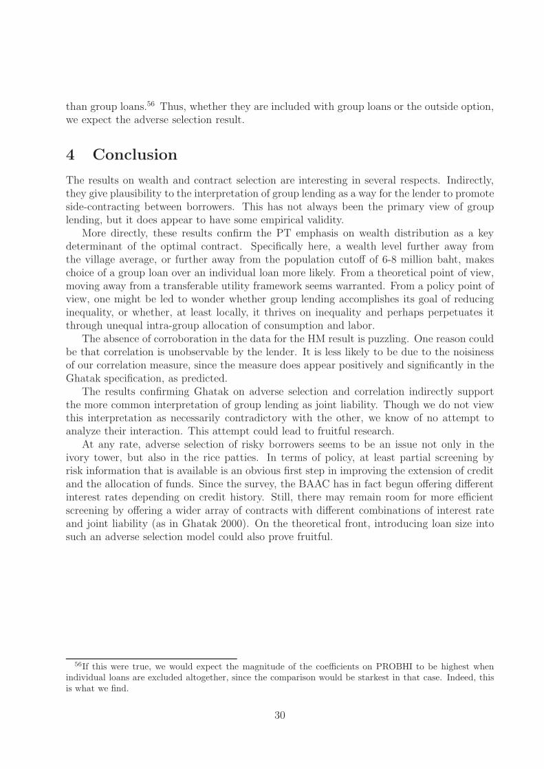
than group loans.56 Thus, whether they are included with group loans or the outside option,we expect the adverse selection result.

4 Conclusion

The results on wealth and contract selection are interesting in several respects. Indirectly,they give plausibility to the interpretation of group lending as a way for the lender to promoteside-contracting between borrowers. This has not always been the primary view of grouplending, but it does appear to have some empirical validity.

More directly, these results confirm the PT emphasis on wealth distribution as a keydeterminant of the optimal contract. Specifically here, a wealth level further away fromthe village average, or further away from the population cutoff of 6-8 million baht, makeschoice of a group loan over an individual loan more likely. From a theoretical point of view,moving away from a transferable utility framework seems warranted. From a policy point ofview, one might be led to wonder whether group lending accomplishes its goal of reducinginequality, or whether, at least locally, it thrives on inequality and perhaps perpetuates itthrough unequal intra-group allocation of consumption and labor.

The absence of corroboration in the data for the HM result is puzzling. One reason couldbe that correlation is unobservable by the lender. It is less likely to be due to the noisinessof our correlation measure, since the measure does appear positively and significantly in theGhatak specification, as predicted.

The results confirming Ghatak on adverse selection and correlation indirectly supportthe more common interpretation of group lending as joint liability. Though we do not viewthis interpretation as necessarily contradictory with the other, we know of no attempt toanalyze their interaction. This attempt could lead to fruitful research.

At any rate, adverse selection of risky borrowers seems to be an issue not only in theivory tower, but also in the rice patties. In terms of policy, at least partial screening byrisk information that is available is an obvious first step in improving the extension of creditand the allocation of funds. Since the survey, the BAAC has in fact begun offering differentinterest rates depending on credit history. Still, there may remain room for more efficientscreening by offering a wider array of contracts with different combinations of interest rateand joint liability (as in Ghatak 2000). On the theoretical front, introducing loan size intosuch an adverse selection model could also prove fruitful.

56If this were true, we would expect the magnitude of the coefficients on PROBHI to be highest whenindividual loans are excluded altogether, since the comparison would be starkest in that case. Indeed, thisis what we find.

30

References

[1] Christian Ahlin and Robert M. Townsend. Using repayment data to test across theoriesof joint liability lending. Working Paper, December 2002.

[2] Lawrence M. Ausubel. Adverse selection in the credit card market. Working Paper,University of Maryland, June 17, 1999.

[3] Pierre-Andre Chiappori, Bruno Jullien, Bernard Salanie, and Francois Salanie. Asym-metric information in insurance: Some testable implications. Working Paper, September16, 2002.

[4] Pierre-Andre Chiappori and Bernard Salanie. Testing contract theory: A survey ofsome recent work. Forthcoming, Advances in Economic Theory.

[5] W. S. Cleveland. Robust locally weighted regression and smoothing scatterplots. Journalof the American Statistical Association, 74:829–836, 1979.

[6] Jianqing Fan. Design-adaptive nonparametric regression. Journal of the AmericanStatistical Association, 87(420):998–1004, December 1992.

[7] Maitreesh Ghatak. Group lending, local information and peer selection. Journal ofDevelopment Economics, 60(1):27–50, October 1999.

[8] Maitreesh Ghatak. Screening by the company you keep: Joint liability lending and thepeer selection effect. Economic Journal, 110(465):601–631, July 2000.

[9] Bengt Holmstrom and Paul Milgrom. Regulating trade among agents. Journal ofInstitutional and Theoretical Economics, 146(1):85–105, March 1990.

[10] Edward Simpson Prescott and Robert M. Townsend. Collective organizations versusrelative performance contracts: Inequality, risk sharing, and moral hazard. Journal ofEconomic Theory, 103(2):282–310, April 2002.

[11] Marguerite S. Robinson. The Microfinance Revolution: Sustainable Finance for thePoor. World Bank, Washington, D.C., 2001.

[12] Joseph E. Stiglitz and Andrew Weiss. Credit rationing in markets with imperfect infor-mation. American Economic Review, 71(3):393–410, June 1981.

[13] Robert M. Townsend and Jacob Yaron. The credit risk-contingency system of an asiandevelopment bank. Federal Reserve Bank of Chicago Economic Perspectives, XXV:31–48, 2001.

[14] Adonis Yatchew. Nonparametric regression techniques in economics. Journal of Eco-nomic Literature, 36:669–721, June 1998.

31