Bulk Dynamics of Droplets in Liquid-Liquid Axial Cyclones

Bu

lk Dyn

amics of D

roplets in

Liqu

id-Liq

uid

Axial C

yclones Laurens van C

ampen

Bulk Dynamics of Droplets in Liquid-Liquid Axial Cyclones

Laurens van Campen9 789064 647369

ISBN 978-90-6464-736-9

Propositionsaccompanying the thesis

Bulk Dynamics of Droplets in Liquid-Liquid Axial CyclonesLaurens van Campen

1. In the optimization process of a liquid-liquid cyclone, aiming at a too high azi-muthal velocity will turn the cyclone into a mixer instead of a phase separator, despite the other design efforts (chapter 7 of this thesis).

2. Without adequate representation of turbulent dispersion in the drop-let equation of motion, it is not possible to predict accurately a liquid- liquid cyclone phase separation efficiency operating at industrial conditions (chapter 6 of this thesis).

3. Liquid-liquid axial cyclones perform best when the swirl element is sized such that in the swirl element the maximum droplet size based on the critical Weber number for the flow is equal to the average size of droplets found upstream of the swirl element (chapter 8 of this thesis).

4. Electric measurements of the phase distribution in media with a high con-ductance should use the free charge carriers instead of a limit on the electric current.

5. The ever-increasing possibilities of numerical simulations of turbulent liquid-liquid flows will not make experimental validation redundant.

6. Designing an experimental facility with strict budget constraints results in the total investigation being more expensive than in case of a design aiming at best performance.

7. The quality of scientific research is inversely proportional to the measure of the business-like look of the university office.

8. Communication between researchers is like a potential barrier: it keeps the researchers apart, while the passage of the barrier leads to more creative and more fruitful interactions.

9. Liberty of choice in the Dutch educational system limits the efficient distribu-tion of labor forces in the Dutch economy.

10. Cognitive understanding of centrifugal acceleration does not lead to success-ful application of these forces during speed skating.

These propositions are regarded as opposable and defendable, and have been approved as such by the supervisors Prof. dr. R.F. Mudde and Prof. dr. ir. H.W.M. Hoeijmakers.

Stellingenbehorende bij het proefschrift

Bulk Dynamics of Droplets in Liquid-Liquid Axial CyclonesLaurens van Campen

1. Bij het optimaliseren van een vloeistof-vloeistof cycloon verandert het streven naar een te hoge azimuthale snelheid de cycloon van een fa-sescheider in een mixer, ongeacht de andere ontwerpinspanningen. (hoofdstuk 7 van dit proefschrift)

2. Zonder toereikende representatie van de turbulente dispersie in de bewe-gingsvergelijking van de druppel is het niet mogelijk om nauwkeurig de fa-sescheiding van een vloeistof-vloeistof cycloon opererend onder industriële omstandigheden te voorspellen. (hoofdstuk 6 van dit proefschrift)

3. Vloeistof-vloeistof axiaal cyclonen presteren het beste wanneer het swirlele-ment zodanig ontworpen is dat in het swirlelement de maximale druppel-grootte gebaseerd op het kritische Weber-getal voor vloeistofstroming gelijk is aan de gemiddelde druppelgrootte stroomopwaarts van het swirlelement. (hoofdstuk 8 van dit proefschrift)

4. Elektrische metingen van de faseverdeling in media met hoge geleidbaarheid kunnen beter de vrije ladingen gebruiken dan de maximale stroom beperken.

5. De immer toenemende mogelijkheden van numeriek onderzoek aan turbu-lente vloeistof-vloeistof stromingen zullen de validatie met resultaten van ex-perimenteel onderzoek nooit overbodig maken.

6. Het ontwerpen van een experimentele opstelling voor een beperkt budget maakt de kosten van het totale onderzoek hoger dan wanneer het ontwerp gebaseerd is op een optimale werking.

7. De kwaliteit van wetenschappelijk onderzoek is omgekeerd evenredig met de mate van zakelijke uitstraling van het universitaire kantoor.

8. Communicatie tussen wetenschappers is als een energiebarrière: van nature zoekt men elkaar niet op, terwijl het doorbreken van de barrière leidt tot crea-tievere en meer vruchtbare interacties.

9. De keuzevrijheid in het Nederlandse onderwijs belemmert een efficiënte al-locatie van arbeidskrachten in onze economie.

10. Het begrip van centrifugale versnelling leidt niet tot het succesvol toepassen van de betreffende krachten bij het schaatsen van bochten.

Deze stellingen worden opponeerbaar en verdedigbaar geacht en zijn als zodanig goedgekeurd door de promotoren Prof. dr. R.F. Mudde en Prof. dr. ir. H.W.M. Hoeijmakers.

i

i

“Thesis1” — 2014/1/7 — 18:22 — page i — #1i

i

i

i

i

i

Bulk Dynamics of Droplets in

Liquid-Liquid Axial Cyclones

i

i

“Thesis1” — 2014/1/7 — 18:22 — page ii — #2i

i

i

i

i

i

i

i

“Thesis1” — 2014/1/7 — 18:22 — page iii — #3i

i

i

i

i

i

Bulk Dynamics of Droplets

in Liquid-Liquid Axial Cyclones

PROEFSCHRIFT

ter verkrijging van de graad van doctor

aan de Technische Universiteit Delft,

op gezag van de Rector Magnificus prof. ir. K.C.A.M. Luyben,

voorzitter van het College van Promoties,

in het openbaar te verdedigen op woensdag 8 januari 2014 om 15:00 uur

door

Laurens Joseph Arnold Marie van Campen

natuurkundig ingenieur

geboren te Nijmegen

i

i

“Thesis1” — 2014/1/7 — 18:22 — page iv — #4i

i

i

i

i

i

Dit proefschrift is goedgekeurd door de promotoren:Prof. dr. R.F. MuddeProf. dr. ir. H.W.M. Hoeijmakers

Samenstelling promotiecommissie:

Rector Magnificus voorzitterProf. dr. R.F. Mudde Technische Universiteit Delft, promotorProf. dr. ir. H.W.M. Hoeijmakers Universiteit Twente, promotorProf. dr. J.G.M. Kuerten Technische Universiteit EindhovenProf. dr. O.J. Nydal Norwegian University of Science and TechnologyProf. dr. ir. B.J. Boersma Technische Universiteit DelftProf. dr. ir. H.E.A. van den Akker Technische Universiteit Delftir. P.H.J. Verbeek FMC TechnologiesProf. dr. ir. C.R. Kleijn Technische Universiteit Delft, reservelid

The work in this thesis is part of project OG-00-004 Development of an Ω2R separatorfocusing on oil/water separation of the Institute for Sustainable Process Technology(ISPT).

Printed by: GVO drukkers & vormgevers B.V. | Ponsen & Looijen, Ede

ISBN 978-90-6464-736-9

Copyright c©2014 by L.J.A.M. van Campen

All rights reserved. No part of the material protected by this copyright notice maybe reproduced or utilized in any form or by any means, electronic or mechanical,including photocopying, recording, or by any information storage and retrieval sys-tem, without written permission from the author.

i

i

“Thesis1” — 2014/1/7 — 18:22 — page v — #5i

i

i

i

i

i

Is the Moon there when nobody looks?David Mermin, 1985

i

i

“Thesis1” — 2014/1/7 — 18:22 — page vi — #6i

i

i

i

i

i

i

i

“Thesis1” — 2014/1/7 — 18:22 — page vii — #7i

i

i

i

i

i

Abstract

Separation of oil and water is an essential step in the treatment of the productionstreams from fossil oil wells. Settling by gravity is a robust though voluminousprocess and therewith expensive method at remote locations, leading to a need forsmaller separation equipment. In this thesis, we describe the research performedon the development of an inline axial cyclone for oil/water separation.This work is part of ISPT project OG-00-004 and has an experimental nature: a flowrig has been constructed to test different cyclones at flow rates up to 60 m3/h in a10 cm diameter tube in which brine and low-viscosity lubricant oil can be mixedin almost any proportion. Results are compared with numerical datasets resultingfrom the same ISPT project.

Three different swirl elements have been developed for this project: a strongswirl element and a weak swirl element with 10 cm diameter, and one element witha 26 cm diameter in combination with a tapered tube section. For all three swirlelements, the velocity profile of water has been measured with Laser Doppler An-emometry (LDA). The strong swirl element has a swirl number of 3.7, the weak of2.3 and the large diameter element of 3.9. The axial velocity profile normalized withthe bulk velocity shows vortex breakdown (upstream flow in the center), where thesevereness of the breakdown normalized with the upstream bulk velocity showsproportionality with the swirl number. For the azimuthal velocity, the velocity pro-file was proportional to the bulk velocity. The non-dimensional azimuthal velocitywas similar for all three swirl elements in the region |r/D| < 0.2. Outside thatregion the relative velocity is strongly influenced by the swirl element.Time series obtained with single phase LDA studies were used to estimate the effectof turbulent dispersion on droplet trajectories. A simplified equation of motionbased on centrifugal buoyancy, drag and turbulent dispersion was solved for manyfictitious droplet paths. The measured, chaotic axial velocity time series was usedto mimic the radial component of the velocity fluctuations. With this model, we canpredict the smallest droplet size that can be separated with a certain cyclone andthe largest droplet size before it is broken by the flow. Model results show goodagreement with overall bulk data obtained in the experimental flow rig.With an intrusive endoscope technique, we measured the droplet size distribution atvarious positions in the axial cyclone. From this, Hinze’s theory for the droplet sizein turbulent pipe flow is confirmed. Furthermore, the inverse correlation betweenazimuthal velocity and median droplet size is shown and quantified: a lower velo-city allows larger droplets to survive.

vii

i

i

“Thesis1” — 2014/1/7 — 18:22 — page viii — #8i

i

i

i

i

i

Different designs were tested to understand which parameters have a large influ-ence on the industrially relevant parameter of separation performance. This ques-tion is answered by variation of the swirl element, swirl tube length, pickup tubediameter, flow rate and droplet size. Changes that affect the droplet size have asevere effect on separation, these are the swirl element and flow rate. Changes thatincrease the droplet size lead to better phase separation. The other geometricalchanges can be used to optimize performance, but are not identified as parametersleading to breakthrough improvements.

Two non-dimensional numbers can be used to explain the behavior of the cyc-lone: the Weber number (We) based on the droplet size upstream of the swirl ele-ment and the maximum velocity obtained in the gaps of the swirl element, and theReynolds number (Reθ) for the droplets downstream of the swirl element based ontheir median diameter and the azimuthal liquid velocity. Separation is better fora smaller We number, because droplets are less vulnerable for breakup under thatcondition. A large Reθ number is beneficial since the droplets then experience alarge centrifugal acceleration which is larger than turbulent dispersion. Both trendsare confirmed with experimental data obtained in this project. We propose thatthere is a function for the maximum possible separation efficiency based on bothnon-dimensional numbers. The inverse coupling between We and Reθ via the azi-muthal velocity makes optimization of separation efficiency difficult. Application ofa large diameter swirl element (low velocity and therefore limited droplet breakup)in combination with a gradual tapering of the tube (increasing the azimuthal velo-city) is a possibility to obtain both a large We and Reθ number. Another option is toplace multiple axial cyclones in series, with a stepwise increase of the swirl strengthin each subsequent cyclone. In such a configuration, each step is capable of separ-ating smaller droplets than the previous step, without immediate breakup of largedroplets. This method should increase the overall quality of the phase separation.

viii

i

i

“Thesis1” — 2014/1/7 — 18:22 — page ix — #9i

i

i

i

i

i

Samenvatting

De scheiding van olie en water is een noodzakelijke stap in de behandeling van devloeistofstroom uit een fossiele oliebron. Scheiding gebaseerd op het uitzakken vande gedispergeerde fase in een zwaartekrachtsveld is een robuust, maar volumineusproces en daardoor duur bij toepassing in installaties op afgelegen locaties zoalsoceanen. Er is daarom behoefte aan kleinere apparatuur voor olie/waterscheiding.In dit proefschrift beschrijven we onderzoek dat we hebben verricht naar de ont-wikkeling van een axiaal cycloon in lijn voor olie/waterscheiding. Dit onderzoekmaakt deel uit van ISPT project OG-00-004 en is experimenteel van aard. Een proef-opstelling is gebouwd om verschillende cyclonen te testen bij debieten oplopend tot60 m3/u in een buis met 10 cm doorsnede. Als werkvloeistoffen werden pekelwa-ter en laag viskeuze smeerolie gebruikt, die in vrijwel elke onderlinge verhoudinggemengd konden worden. De experimentele resultaten zijn vergeleken met nume-rieke data die verkregen waren binnen hetzelfde ISPT project.

Drie verschillende swirlelementen zijn ontwikkeld voor dit project: een sterk enzwak element, met elk 10 cm diameter en een groot element met een diameter van26 cm. Dit laatste element werd gecombineerd met een toelopend buisdeel om hetaan te sluiten op de 10 cm buis met roterende stroming. Voor alle drie de ele-menten hebben we het snelheidsprofiel gemeten met Laser Doppler Anemometrie(LDA). Het sterke swirlelement heeft een swirlgetal van 3,7, het zwakke van 2,3 enhetgrote van 3,9. Alle drie de snelheidsprofielen vertonen het vortex breakdownverschijnsel. De met de bulksnelheid genormaliseerde snelheidsprofielen vertonenevenredigheid met het swirlgetal. De azimuthale snelheid is voor elk swirlelementrecht evenredig met de bulksnelheid stroomopwaarts van het swirlelement. Hetazimuthale snelheidsprofiel gedeeld op de bulksnelheid was voor elk van de drieswirlelementen gelijk in het gebied |r/D|<0.2. Buiten dat gebied heeft het swirl-element sterke invloed op de azimuthale snelheid.Op basis van de met LDA verkregen lokale snelheid als functie van de tijd hebbenwe het effect bekeken van turbulente dispersie. We gebruikten een versimpeldebewegingsvergelijking, gebaseerd op de centrifugaal opwaartse kracht, wrijving enturbulente dispersie, om druppelpaden op te lossen voor veel fictieve druppels. Demiddels metingen verkregen tijdseries van de axiale snelheid, met een turbulentkarakter, werden gebruikt om de snelheidsfluctuaties in de radiële richting na tebootsen. Het model voorspelt de grootte van de kleinste druppels die afgeschei-den kunnen worden met een bepaald type cycloon en ook de maximale grootte van

ix

i

i

“Thesis1” — 2014/1/7 — 18:22 — page x — #10i

i

i

i

i

i

druppels voordat ze door de vloeistofstroming zullen worden opgebroken. De re-sultaten van het model komen goed overeen met de rendementsdata gemeten in deexperimentele opstelling.De druppelgrootteverdeling is gemeten met een endoscoop welke op verschillendeplaatsen in de buis met de roterende stroming is gestoken. De theorie van Hinze,die de druppelgrootte voorspelt voor een turbulente pijpstroming, is hiermee ge-valideerd voor onze opstelling. Verder tonen de metingen de inverse relatie aantussen de azimuthale snelheid en de mediaan van de druppelgrootte, waarvoorwe een kwantitatief voorspellend model voorstellen: een lage snelheid laat grotedruppels overleven.

Verschillende ontwerpen zijn getest om grip te krijgen op de grootheden die vanbelang zijn bij het ontwerpen van cyclonen voor toepassing in de industrie. Geva-rieerde parameters zijn: het swirlelement, lengte van de swirlbuis, diameter van deopvangbuis voor de lichte fase, debiet en druppelgrootte. Elke verandering die dedruppelgrootte beïnvloedt, heeft een groot effect op het scheidingsrendement: ver-anderingen die leiden tot grotere druppels leiden tot een betere fasescheiding. Deandere geometrieveranderingen hebben wel invloed op het scheidingsrendement,maar zullen niet tot schokkende verbeteringen leiden in de fasescheiding.

Het gedrag van onze cycloon kan ook worden gevat in twee niet-dimensionelekentallen: het Webergetal (We), gekozen voor druppels met de grootte stroomop-waarts van het swirlelement met de snelheid die ze zullen halen ter hoogte vanhet swirlelement, en het Reynoldsgetal (Reθ) gedefinieerd voor druppels stroomaf-waarts van het swirlelement met hun azimuthale snelheid en de mediaan van hundruppelgrootte. Een kleiner We-getal leidt tot betere scheiding, omdat druppelsdan minder gevoelig zijn voor opbreking. Een groter Reθ-getal is gunstig: de drup-pels ervaren dan een centrifugale versnelling die de turbulente dispersieve effectenbeter overwint. Beide trends worden bevestigd met experimentele data verkregenin dit project, en we stellen voor dat elk getal de afhankelijke is van een functie diede maximaal haalbare scheiding begrenst. Vanwege de inverse koppeling tussenhet Weber- en Reynoldsgetal via de azimuthale snelheid, is het maximaliseren vanhet scheidingsrendement erg moeilijk. Het toepassen van een swirlelement met gro-te diameter (lage snelheid en dus druppelafbreking), gevolgd door een geleidelijkevernauwing van de swirlbuis (verhoogt de azimuthale snelheid) is een mogelijkheidom zowel het We- als het Reθ-getal groot te maken. Een andere optie is om cyclo-nen in serie te zetten met in elke opvolgende stap een toenemende swirlsterkte. Zoscheid je steeds kleinere druppeltjes af, zonder in de eerste stap de grote druppelsdirect kapot te breken.

x

i

i

“Thesis1” — 2014/1/7 — 18:22 — page xi — #11i

i

i

i

i

i

Contents

Abstract vii

Samenvatting ix

Nomenclature xv

1 Introduction 1

1.1 Need for cyclones . . . . . . . . . . . . . . . . . . . . . . . . . . . . . . . 11.1.1 Crude oil production . . . . . . . . . . . . . . . . . . . . . . . . . 11.1.2 Oil extraction . . . . . . . . . . . . . . . . . . . . . . . . . . . . . 11.1.3 Cyclones are compact . . . . . . . . . . . . . . . . . . . . . . . . 2

1.2 Characterization of cyclones . . . . . . . . . . . . . . . . . . . . . . . . . 31.3 Previous work . . . . . . . . . . . . . . . . . . . . . . . . . . . . . . . . . 41.4 Project organization . . . . . . . . . . . . . . . . . . . . . . . . . . . . . . 41.5 Present work . . . . . . . . . . . . . . . . . . . . . . . . . . . . . . . . . . 5

2 Experimental facility for oil/water flow 7

2.1 Dimensions and scaling . . . . . . . . . . . . . . . . . . . . . . . . . . . 72.2 Description of the parts . . . . . . . . . . . . . . . . . . . . . . . . . . . 82.3 Operating procedures . . . . . . . . . . . . . . . . . . . . . . . . . . . . 14

2.3.1 Startup . . . . . . . . . . . . . . . . . . . . . . . . . . . . . . . . . 152.3.2 Operating window . . . . . . . . . . . . . . . . . . . . . . . . . . 152.3.3 Shutdown . . . . . . . . . . . . . . . . . . . . . . . . . . . . . . . 152.3.4 Maintenance operations . . . . . . . . . . . . . . . . . . . . . . . 18

2.4 Consistency of results . . . . . . . . . . . . . . . . . . . . . . . . . . . . 182.4.1 Reproducibility . . . . . . . . . . . . . . . . . . . . . . . . . . . . 18

2.5 Durability of the process liquids . . . . . . . . . . . . . . . . . . . . . . 222.5.1 Possible causes . . . . . . . . . . . . . . . . . . . . . . . . . . . . 23

2.6 Facility for rotating swirl element . . . . . . . . . . . . . . . . . . . . . 282.7 Conclusion . . . . . . . . . . . . . . . . . . . . . . . . . . . . . . . . . . . 28

3 Experimental methods 31

3.1 Laser Doppler Anemometry . . . . . . . . . . . . . . . . . . . . . . . . . 313.1.1 LDA apparatus . . . . . . . . . . . . . . . . . . . . . . . . . . . . 313.1.2 Measurement volume . . . . . . . . . . . . . . . . . . . . . . . . 323.1.3 Tracer particles . . . . . . . . . . . . . . . . . . . . . . . . . . . . 32

xi

i

i

“Thesis1” — 2014/1/7 — 18:22 — page xii — #12i

i

i

i

i

i

3.1.4 Traversing system . . . . . . . . . . . . . . . . . . . . . . . . . . 343.1.5 Void kernel . . . . . . . . . . . . . . . . . . . . . . . . . . . . . . 35

3.2 Numerical method . . . . . . . . . . . . . . . . . . . . . . . . . . . . . . 353.2.1 Single Phase . . . . . . . . . . . . . . . . . . . . . . . . . . . . . . 363.2.2 Two Phase Flow . . . . . . . . . . . . . . . . . . . . . . . . . . . . 36

3.3 Efficiency measurements . . . . . . . . . . . . . . . . . . . . . . . . . . . 373.4 Droplet sizing . . . . . . . . . . . . . . . . . . . . . . . . . . . . . . . . . 37

3.4.1 Direct photography with an endoscope . . . . . . . . . . . . . . 383.4.2 Liquid sampling and off-line analysis . . . . . . . . . . . . . . . 423.4.3 Glass fiber sensor . . . . . . . . . . . . . . . . . . . . . . . . . . . 453.4.4 Comparison of methods . . . . . . . . . . . . . . . . . . . . . . . 47

3.5 A novel capacitance based wiremesh technique . . . . . . . . . . . . . 473.5.1 Introduction . . . . . . . . . . . . . . . . . . . . . . . . . . . . . . 473.5.2 Geometry . . . . . . . . . . . . . . . . . . . . . . . . . . . . . . . 493.5.3 Electric fields . . . . . . . . . . . . . . . . . . . . . . . . . . . . . 493.5.4 Measurement circuit . . . . . . . . . . . . . . . . . . . . . . . . . 523.5.5 Fluid-sensor interaction . . . . . . . . . . . . . . . . . . . . . . . 553.5.6 Visualization of an oil kernel . . . . . . . . . . . . . . . . . . . . 553.5.7 Discussion and Conclusion . . . . . . . . . . . . . . . . . . . . . 56

4 Strength of generated swirl 59

4.1 Theory . . . . . . . . . . . . . . . . . . . . . . . . . . . . . . . . . . . . . 594.1.1 Force balances . . . . . . . . . . . . . . . . . . . . . . . . . . . . . 594.1.2 Droplet elongation . . . . . . . . . . . . . . . . . . . . . . . . . . 624.1.3 Time scales . . . . . . . . . . . . . . . . . . . . . . . . . . . . . . 62

4.2 Swirl element design . . . . . . . . . . . . . . . . . . . . . . . . . . . . . 654.2.1 Strong swirl element . . . . . . . . . . . . . . . . . . . . . . . . . 654.2.2 Weak swirl element . . . . . . . . . . . . . . . . . . . . . . . . . 714.2.3 Large swirl element . . . . . . . . . . . . . . . . . . . . . . . . . 724.2.4 Tapered tube section . . . . . . . . . . . . . . . . . . . . . . . . . 74

4.3 Profile of the swirling flow . . . . . . . . . . . . . . . . . . . . . . . . . 754.3.1 Experimental conditions . . . . . . . . . . . . . . . . . . . . . . . 774.3.2 Strong swirl element . . . . . . . . . . . . . . . . . . . . . . . . . 77

4.4 Properties of swirling flow . . . . . . . . . . . . . . . . . . . . . . . . . . 794.4.1 Vortex decay . . . . . . . . . . . . . . . . . . . . . . . . . . . . . . 794.4.2 Precessing Vortex Core . . . . . . . . . . . . . . . . . . . . . . . 804.4.3 Detail at the pick-up tube . . . . . . . . . . . . . . . . . . . . . . 81

4.5 Influence of operational parameters . . . . . . . . . . . . . . . . . . . . 844.5.1 Flow split effect . . . . . . . . . . . . . . . . . . . . . . . . . . . . 844.5.2 Effect of flow rate . . . . . . . . . . . . . . . . . . . . . . . . . . . 87

4.6 Conclusion . . . . . . . . . . . . . . . . . . . . . . . . . . . . . . . . . . . 884.6.1 Prediction of the velocity profile . . . . . . . . . . . . . . . . . . 894.6.2 Operational effects on phase separation . . . . . . . . . . . . . . 91

5 Dispersed droplets in dilute swirling flow 93

5.1 Theory . . . . . . . . . . . . . . . . . . . . . . . . . . . . . . . . . . . . . 935.2 Droplet model . . . . . . . . . . . . . . . . . . . . . . . . . . . . . . . . . 98

xii

i

i

“Thesis1” — 2014/1/7 — 18:22 — page xiii — #13i

i

i

i

i

i

5.2.1 Equation of motion . . . . . . . . . . . . . . . . . . . . . . . . . . 985.2.2 Experimental input to the model . . . . . . . . . . . . . . . . . . 995.2.3 Numerical implementation . . . . . . . . . . . . . . . . . . . . . 1015.2.4 Droplet break-up . . . . . . . . . . . . . . . . . . . . . . . . . . . 103

5.3 Dilute droplets simulation results . . . . . . . . . . . . . . . . . . . . . 1045.3.1 Smallest separated droplets . . . . . . . . . . . . . . . . . . . . . 1065.3.2 Droplet break-up . . . . . . . . . . . . . . . . . . . . . . . . . . . 1065.3.3 Separation window . . . . . . . . . . . . . . . . . . . . . . . . . . 110

5.4 Conclusions . . . . . . . . . . . . . . . . . . . . . . . . . . . . . . . . . . 1115.5 Outlook . . . . . . . . . . . . . . . . . . . . . . . . . . . . . . . . . . . . . 113

6 Droplet break-up and coalescence 115

6.1 Droplet size upstream of the swirl element . . . . . . . . . . . . . . . . 1156.1.1 Turbulent liquid-liquid pipe flow . . . . . . . . . . . . . . . . . 1156.1.2 Droplet size reduction with valves . . . . . . . . . . . . . . . . . 117

6.2 Droplet size reduction with a swirl element . . . . . . . . . . . . . . . . 1176.2.1 Model of the break-up in a swirl element . . . . . . . . . . . . . 1176.2.2 Experimental results . . . . . . . . . . . . . . . . . . . . . . . . . 120

6.3 Droplet coalescence inside the cyclone . . . . . . . . . . . . . . . . . . . 1236.4 Conclusion . . . . . . . . . . . . . . . . . . . . . . . . . . . . . . . . . . . 125

7 Analysis of swirl separation performance 127

7.1 Geometric optimization . . . . . . . . . . . . . . . . . . . . . . . . . . . 1277.1.1 Swirl element type . . . . . . . . . . . . . . . . . . . . . . . . . . 1277.1.2 Swirl tube length . . . . . . . . . . . . . . . . . . . . . . . . . . . 1287.1.3 Pick-up tube diameter . . . . . . . . . . . . . . . . . . . . . . . . 130

7.2 Operational optimization . . . . . . . . . . . . . . . . . . . . . . . . . . 1327.2.1 Flow split . . . . . . . . . . . . . . . . . . . . . . . . . . . . . . . 1327.2.2 Flow rate . . . . . . . . . . . . . . . . . . . . . . . . . . . . . . . . 1357.2.3 Droplet size . . . . . . . . . . . . . . . . . . . . . . . . . . . . . . 1417.2.4 Phase inversion . . . . . . . . . . . . . . . . . . . . . . . . . . . . 141

7.3 Static versus Rotating element . . . . . . . . . . . . . . . . . . . . . . . . 1447.4 Conclusion . . . . . . . . . . . . . . . . . . . . . . . . . . . . . . . . . . . 144

8 Design considerations for Liquid-Liquid Cyclones 147

8.1 Scaling parameters . . . . . . . . . . . . . . . . . . . . . . . . . . . . . . 1478.1.1 Reynolds number . . . . . . . . . . . . . . . . . . . . . . . . . . . 1478.1.2 Weber number . . . . . . . . . . . . . . . . . . . . . . . . . . . . 148

8.2 Prediction of current swirl elements . . . . . . . . . . . . . . . . . . . . 1498.2.1 Method . . . . . . . . . . . . . . . . . . . . . . . . . . . . . . . . . 1498.2.2 Reynolds depends on Weber . . . . . . . . . . . . . . . . . . . . 1498.2.3 Optimal point of operation . . . . . . . . . . . . . . . . . . . . . 1518.2.4 Dependence on droplet size . . . . . . . . . . . . . . . . . . . . . 151

8.3 Guide on cyclone design . . . . . . . . . . . . . . . . . . . . . . . . . . . 1518.3.1 Input parameters . . . . . . . . . . . . . . . . . . . . . . . . . . . 1538.3.2 Single cyclone design . . . . . . . . . . . . . . . . . . . . . . . . 1538.3.3 Multi-stage cyclone design . . . . . . . . . . . . . . . . . . . . . 154

xiii

i

i

“Thesis1” — 2014/1/7 — 18:22 — page xiv — #14i

i

i

i

i

i

8.3.4 Sizing . . . . . . . . . . . . . . . . . . . . . . . . . . . . . . . . . . 1568.3.5 Process control . . . . . . . . . . . . . . . . . . . . . . . . . . . . 1598.3.6 Swirl element design . . . . . . . . . . . . . . . . . . . . . . . . . 159

8.4 Concluding remarks . . . . . . . . . . . . . . . . . . . . . . . . . . . . . 159

Bibliography 161

A Description of swirling flow 165

A.1 Governing equations . . . . . . . . . . . . . . . . . . . . . . . . . . . . . 165A.2 Empirical description of swirling flow . . . . . . . . . . . . . . . . . . . 166A.3 Swirl number . . . . . . . . . . . . . . . . . . . . . . . . . . . . . . . . . 167A.4 Advanced concepts . . . . . . . . . . . . . . . . . . . . . . . . . . . . . . 168

A.4.1 Vortex Breakdown and flow reversal . . . . . . . . . . . . . . . . 168A.4.2 Time-independent instabilities . . . . . . . . . . . . . . . . . . . 168

B Estimation of turbulence parameters 171

B.1 Turbulence . . . . . . . . . . . . . . . . . . . . . . . . . . . . . . . . . . . 171B.2 Method . . . . . . . . . . . . . . . . . . . . . . . . . . . . . . . . . . . . . 172B.3 Result . . . . . . . . . . . . . . . . . . . . . . . . . . . . . . . . . . . . . . 173

C Uncertainty analysis 175

C.1 Accuracy of the measurement equipment . . . . . . . . . . . . . . . . . 175C.2 Oil Concentration in outputs . . . . . . . . . . . . . . . . . . . . . . . . 176

D Drag relation for a sphere 179

List of publications 181

Acknowledgements 183

Curriculum Vitae 187

xiv

i

i

“Thesis1” — 2014/1/7 — 18:22 — page xv — #15i

i

i

i

i

i

Nomenclature

Roman Symbols

Symbol Description S.I. units

A Area (m2)B Magnetic induction (N/Am)C Electrical capacity (C/V)D Electric displacement (C/m2)Cd Empirical swirl decay parameter (-)CD Drag coefficient (-)D Tube diameter (-)Dd Droplet diameter (m)D f Diameter of flow area (m)E Electric field (V/m)Fb Buoyancy force (N)Fc Centrifugal force (N)Fd Drag force (N)I Electrical current (A)J Bessel function (-)J Impulse (Ns)Jd Displacement current (A/m2)L Angular momentum (kg m2/s)L Length (m)R Electrical Resistance (Ω)U Electric potential (V)V Electrical potential difference (V)Vd Droplet Volume (m3)a Sphere radius for light scattering (m)c Volumetric oil Concentration (-)d Inter-plane distance (m)de−2 Diameter of incoming laser beam (m)f Focal length (m)g Gravity constant (m/s2)k Wave Number (1/m)

xv

i

i

“Thesis1” — 2014/1/7 — 18:22 — page xvi — #16i

i

i

i

i

i

Roman Symbols (continued)


kg Geometry factor (m)ℓ Turbulent eddy size (m)md Droplet mass (kg)n Refractive index (-)

Particle size distribution (-)p Pressure (Pa)p Momentum (kg m/s)r Radial position (m)rp Radial position of a droplet (m)t Shear (N/m2)u continuous phase velocity (m/s)uθ azimuthal component of the continuous

phase(m/s)

ur radial component of the continuous phase (m/s)uz axial component of the continuous phase (m/s)v Particle velocity (m/s)vθ Tangential component of the particle ve-

locity(m/s)

vr Radial component of the particle velocity (m/s)vz Axial component of the particle velocity (m/s)vr radial velocity (m/s)vθ azimuthal velocity (m/s)vterm terminal velocity (m/s)vz axial velocity (m/s)w Wire distance (m)

xvi

i

i

“Thesis1” — 2014/1/7 — 18:22 — page xvii — #17i

i

i

i

i

i

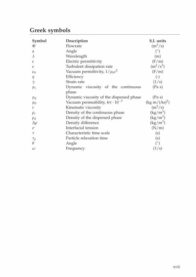
Greek symbols


Φ Flowrate (m3/s)α Angle ()λ Wavelength (m)ǫ Electric permittivity (F/m)ǫ Turbulent dissipation rate (m2/s3)ǫ0 Vacuum permittivity, 1/µ0c2 (F/m)η Efficiency (-)γ Strain rate (1/s)µc Dynamic viscosity of the continuous

phase(Pa s)

µd Dynamic viscosity of the dispersed phase (Pa s)µ0 Vacuum permeability, 4π · 10−7 (kg m/(As)2)ν Kinematic viscosity (m2/s)ρc Density of the continuous phase (kg/m3)ρd Density of the dispersed phase (kg/m3)∆ρ Density difference (kg/m3)σ Interfacial tension (N/m)τ Characteristic time scale (s)τp Particle relaxation time (s)θ Angle ()ω Frequency (1/s)

xvii

i

i

“Thesis1” — 2014/1/7 — 18:22 — page xviii — #18i

i

i

i

i

i

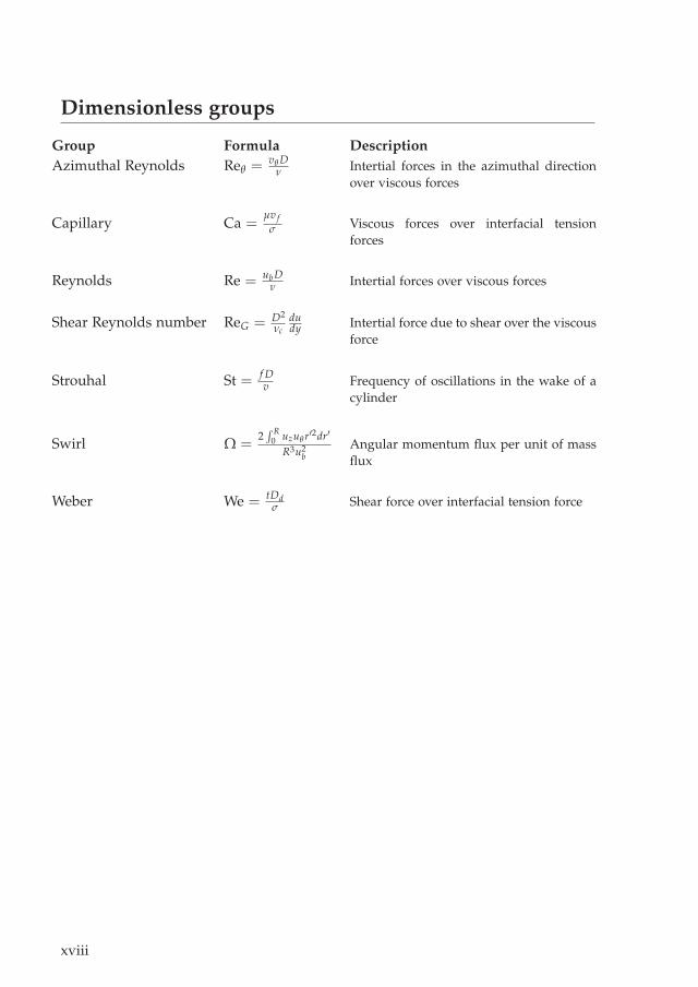
Dimensionless groups

Group Formula Description

Azimuthal Reynolds Reθ = vθ Dν Intertial forces in the azimuthal direction

over viscous forces

Capillary Ca =µv f

σ Viscous forces over interfacial tensionforces

Reynolds Re = ubDν Intertial forces over viscous forces

Shear Reynolds number ReG = D2

νc

dudy Intertial force due to shear over the viscous

force

Strouhal St = f Dv Frequency of oscillations in the wake of a

cylinder

Swirl Ω =2∫ R

0 uzuθr′2dr′

R3u2b

Angular momentum flux per unit of massflux

Weber We = tDdσ Shear force over interfacial tension force

xviii

i

i

“Thesis1” — 2014/1/7 — 18:22 — page xix — #19i

i

i

i

i

i

Abbreviations

Name Description

AISI American Iron and Steel InstitueCFD Computational Fluid DynamicsCFX Commercial CFD solverDC Direct CurrentEPDM Ethylene Propylene Diene MonomerFS Flow SplitGC Gas ChromatogramHPO Heavy Phase OutletHZDR Helmholtz Zentrum Dresden RossendorfISPT Institute for Sustainable Process TechnologyLDA Laser Doppler AnemometryLPO Light Phase OutletMSDS Material Safety Data SheetNaCl Natrium Chloride (table salt)NBR Nitrile Butadiene RubberPMMA Poly Methyl MethAcrylate (polymer)PP Poly Propylene (polymer)PTFE Poly Tetra Fluoro Ethylene (Teflon)PVC Poly Vinyl Chloride (polymer)RSM Reynolds Stress ModelSDS Sodium Dodecyl Sulfate (surfactant)

xix

i

i

“Thesis1” — 2014/1/7 — 18:22 — page xx — #20i

i

i

i

i

i

i

i

“Thesis1” — 2014/1/7 — 18:22 — page 1 — #21i

i

i

i

i

i

CHAPTER 1

Introduction

1.1 Need for cyclones

1.1.1 Crude oil production

Since the modern age discovery of fossil oil as illumination fluid by Edwin Drakein 1859 [1], both production and consumption of fossil fuels have grown to a levelat which present day society cannot exist without. The extensive exploration of oilfields first focussed on “easy oil”, being shallow fields that are onshore and whichare pressurized enough to produce liquids without additional aid. Nowadays,crude production has shifted to remote onshore locations and mainly off shoredeep-water locations, where advanced techniques are deployed to retrieve as muchcrude as possible from the fields.

1.1.2 Oil extraction

Oil is formed in the subsurface by conversion of organic material under anaerobicconditions. Due to its low density compared with soil material as well as water,buoyancy moves the oil to the surface. Only if an impermeable material is presentin a dome shape that can capture the rising liquid, the oil is trapped underneath.Water present in the soil is in general also less dense compared with its surround-ings, and rises as well. Due to the density difference between oil and water, wetypically find oil underneath an impermeable salt formation with water below theoil. Figure 1.1 depicts such a geological system. The regions indicated with “oil”and “water” are porous rocks containing the liquids.

To produce oil from a field as in figure 1.1, a well is drilled. Due to the over-pressure, oil flows into the vertical tube. Mature fields, which are at lower pressure,are often mechanically assisted, for example using pumpjacks. Due to the viscositydifference of oil and water, water is more mobile as a result of which water ‘fingers’around the oil and flows into the wellbore before all oil is produced. Due to thisphenomenon, most of the time a mixture of oil and water is produced from the oil

1

i

i

“Thesis1” — 2014/1/7 — 18:22 — page 2 — #22i

i

i

i

i

i

2 Chapter 1. Introduction

oil

water

impermeable rock

soil material

sea

production platform

Figure 1.1: Schematic of a sub-sea oil field.

well, which requires separation in downstream process equipment.Two current developments in the production of crude oil lead to a demand fornew separation equipment: (i) an increasing amount of fossil fuels is producedoffshore, with a high constructional cost of the platform and (ii) fields are producedfor a longer period of time, leading to higher water concentrations (water cuts).From an economical perspective, it is desirable to separate the oil and water flowclose to the well to avoid costs for transportation of non-commercial water. Typicalrequirements for the downstream side of the separation process is to have less than30 ppm oil in water (legal limit to dump it overboard) and to have less than 0.5 %vol. water in oil (acceptable limit for a refinery).

1.1.3 Cyclones are compact

For bulk separation, the density difference between oil and water is a suitable phys-ical property to exploit. The conventional way is to employ a large vessel, in whichthe residence time under continuous operation is long enough to allow separationof phases by gravity. The required large size to meet the requirements discussed inthe preceding section leads to high investments in offshore separation equipment.Cyclones use centrifugal acceleration to separate phases with a different density, inwhich the acceleration can be orders of magnitude larger than that of gravity. Cyc-lones are therefore a promising alternative for the bulky gravity-based separationequipment.

i

i

“Thesis1” — 2014/1/7 — 18:22 — page 3 — #23i

i

i

i

i

i

1.2. Characterization of cyclones 3

1.2 Characterization of cyclones

Cyclones are used in many different fields for various combinations of phases. Theresearch on cyclones typically focuses on a specific combination of phases:

• gas/solid;

• gas/liquid;

• liquid/solid;

• liquid/liquid.

Although the underlying physics is similar for all of these combinations, there aredifferences. A liquid cyclone is less turbulent due to the higher viscous forces,though the interfacial chemistry between the phases can cause liquid-liquid emul-sions. A gas cyclone typically has the advantage of a large density difference,though a risk for gas/liquid emulsions (foam). A cyclone with a solid dispersedphase cannot suffer from break-up effects, although there can be attrition.There are some design choices that make a significant difference for the type ofcyclone:

• Inlet geometry:

– tangential: the input stream is typically distributed over multiple tubesthat are tangentially connected to the cyclone, equidistantly distributedover the circumference;

– axial: a static swirl element with vanes accelerates the liquid in azimuthaldirection;

• Swirl tube geometry:

– traditional: a shape with a conical-shaped reduction of the tube diameterfrom inlet to outlet of the heavy phase; this is the typical shape of ahydrocyclone;

– cylindrical: no diameter reduction of the tube diameter - this design isadopted to reduce the required space of a cyclone;

• Flow direction:

– counter current: the heavy phase outlet (HPO) is at the downstreamside, the light phase outlet (LPO) at the upstream side (as seen from theinflow);

– co-current: both outlets are positioned at the downstream side.

i

i

“Thesis1” — 2014/1/7 — 18:22 — page 4 — #24i

i

i

i

i

i


1.3 Previous work

The first cyclone aimed at phase separation was patented in 1891 by Bretney [2].Extensive use, however, did not start before the 1950s [3]. The use of cyclonesfor removal of solid particles from a gas stream was the first major application.The large density difference and the particles being solid makes the separation ofthese streams relatively easy. The next development step were gas-liquid cyclones,for which the density difference is large, but additional difficulties are introducedthrough the possible breakup of droplets. The first application for liquid-liquidflow dates back to around 1980 (see Colman et al. [4]). The earlier systems hada traditional cyclone design, with tangential inlets, a conical body and counter-current flow. Dirkzwager [3] introduced an axial cyclone with a static in-line swirlelement to decrease the turbulence production and pressure drop. However, hisresearch was limited to single phase flow only.In recent years, the research focused on different aspects. Numerical work con-centrated on single phase cyclones in order to understand the flow phenomenaoccurring in the strong vortex flows. These results are compared with experiment-ally obtained data, e.g. Lu et al. [5], who applied a Reynolds stress model andcompared predicted results with laser Doppler measurements. Also multiphasenumerical work is conducted, e.g. Paladino et al. [6], Noroozi and Hashemabadi[7], Schütz et al. [8], Amini et al. [9], usually the comparison with experimental datawas limited to the separation efficiency, but discrepancies were not understood.Experimental studies focused primarily on the optimization of the separator design.For example Young et al. [10] carried out an optimization study of the separatordimensions, Oropeza-Vazquez et al. [11] proposes a cylindrical geometry with azi-muthally positioned inlets and Husveg et al. [12] examines the cyclonic separatorefficiency as function of the liquid intake.

1.4 Project organization

The work described in this thesis is part of Institute for Sustainable Process Tech-nology (ISPT) project OG-00-004 “Development of an Ω2R separator focusing onoil/water separation” in which four industrial partners (FMC Separation Systems,Frames Separation Technologies, Shell and Wintershall) cooperate with three uni-versities (Delft University of Technology, University of Twente and WageningenUniversity). The project aims at increasing the understanding of the physics in-volved in liquid-liquid axial cylindrical cyclones and using this knowledge to testdesign improvements.

Previous work did not fully resolve the fundamental of liquid-liquid cycloneslagging behind compared to gas-solid and gas-liquid cyclones. Two phenomenamake an accurate prediction of the flow in a liquid-liquid cyclone difficult: (i) effectsof turbulence in the strong (non-isotropic) swirling flow is difficult to model and

i

i

“Thesis1” — 2014/1/7 — 18:22 — page 5 — #25i

i

i

i

i

i

1.5. Present work 5

(ii) the breakup and coalescence of droplets is not fully understood, let alone thatpredictions can be made for millions of droplets in a cyclone. A direct numericalsimulation is well beyond the capability of current computing power, with smallestscales to be resolved in the µm range and the integral scale in the meter range.

This project therefore exploits different means to gain understanding of cyclonesand to improve design. At Twente University, PhD student Slot [13] performednumerical single and multiphase work on the design of the axial cylindrical cyclonesused in the present thesis, the resulting fluid flow and on predicting separation withthe Euler-Euler approach. The lack of a decent model of droplet break-up and ofcoalescence and turbulent dispersion hamper the accuracy of the results of thesesimulations. A postdoc in Wageningen (see Krebs et al. [14]) performed detailedexperimental studies on droplet-droplet collisions and droplet breakup. This servedas input for the numerical work in Twente. The present thesis presents the bulkseparation; these results were compared to the separation process data discussed inthe Twente thesis. The final conclusions aim at improved understanding of dropletbreak-up and coalescence effects in a physical bulk separation system system, aswell as improved understanding of the effects of turbulent dispersion on phaseseparation.

1.5 Present work

Chapters 2 and 3 of this thesis introduce the flow rig and the experimental methodsused to examine the flow. Results are ordered in the next four chapters.

Swirl The coupling between the static swirl element and resulting fluid flow isan important factor for the understanding and prediction of the performance ofcyclones. In chapter 4 both the design and the resulting fluid flow are investig-ated. Furthermore, various sources in literature [3, 15, 16, 17] indicate the unsteadyand non-axi-asymmetric nature of swirling flows. Based on the velocity data ofchapter 4 the time-dependencies involved in the system used during this researchare discussed.

Turbulence Balancing only centrifugal buoyancy and drag results in a finite ter-minal velocity in the radial direction for all droplets, which would enable perfectseparation. Turbulent dispersion, however, disturbs separation. Chapter 5 quanti-fies the effect of turbulence based on the single-phase, experimental LDA data fromchapter 4. We relate the smallest captured droplet size to the swirl strength.

Droplet size Acceleration of droplets and shear in liquids affect the maximumstable droplet size and therewith the droplet size distribution. Since both accel-eration and shear are present in cyclones, droplets will be broken. In chapter 6the droplet break up is quantified, based on liquid velocity and swirl strength, atdifferent locations upstream, downstream and inside the cyclone.

i

i

“Thesis1” — 2014/1/7 — 18:22 — page 6 — #26i

i

i

i

i

i


Design Chapter 7 evaluates a selected set of design parameters, such as diameterand vane angle. The effects of these variations are compared based on separationefficiency, from which for each parameter the importance in the design process isdeduced. The work in this chapter has a somewhat empirical nature, since not allmechanisms are completely understood. Only the effect on separation is evaluated.

Results of the four preceding chapters are combined in chapter 8 to provide rulesfor the design of axial cyclones. The most important conclusion links the dropletbreakup by acceleration to the required azimuthal velocity to achieve adequate sep-aration, based on a non-dimensionalized dataset.

i

i

“Thesis1” — 2014/1/7 — 18:22 — page 7 — #27i

i

i

i

i

i

CHAPTER 2

Experimental facility for oil/water flow

This chapter describes the experimental facility built for the investigations presen-ted in this thesis. It serves as a reference for the other chapters.All parts of the experimental rig are introduced, we describe the typical measure-ment procedure, the resulting droplet size upstream of the swirl generation and theaccuracy of the results. The design of the measurement section is not part of thischapter, but is extensively discussed in chapter 3.

2.1 Dimensions and scaling

A flow rig was constructed to investigate the swirl based separation process. Therig used in this project is located in the Kramers Laboratory, Prins Bernhardlaan 6in Delft. The rig was designed to test the separation characteristics of an industri-ally relevant system. Since no standards exist for industrially relevant flows, thefollowing choices were made:

Bulk velocity: 2.0 m/sTube diameter: 100 mmWorking fluids: brine (9 wt% NaCl)

mineral oil

Brine is used instead of water to provide more realistic field conditions and to allowcomparison with Shell’s Multiphase Test Facility in Rijswijk (The Netherlands). Thebroad range in viscosity of mineral oils requires a further narrowing down of thespecifications. Tests with oils having a kinematic viscosity up to 150 mm2/s shouldbe possible. The setup was designed such that the oil fraction fed to the system canrange from 0 to 1.The choices above provide the requirements for the material selection, pump capa-city and downstream separation specifications. The main construction materials arePoly Vinyl Chloride (PVC) and stainless steel AISI 316L. Both materials are resist-ant to mineral oil as well as brine. The main tubing is made out of PVC, due to

7

i

i

“Thesis1” — 2014/1/7 — 18:22 — page 8 — #28i

i

i

i

i

i

8 Chapter 2. Experimental facility for oil/water flow

Pressure relief valve

Float owmeter

Coriolis owmeter

Pneumatic butter y valve

Butter y valve

Breathing valve

Membrane valve

Pneumatic membrane valve

Ball valve

Swirl element

Flow straightener

Sieving plate

Centrifugal pump

Figure 2.1: Scheme of the flow rig, status during the final experiments.

its relatively low price compared to stainless steel and good machining qualities.Pumps, valves and other appendages are made out of stainless steel AISI 316L. Inthe subsequent sections the various parts of the rig are discussed.One of the process liquids is brine, a solution of 9 wt% NaCl in tap water. Dueto the electric conductivity and especially the presence of Cl− ions, brine promotescorrosion of metals.

2.2 Description of the parts

Figure 2.1 presents a chart of the flow rig. This section describes the parts in therig, starting with the storage vessels, continuing in the streamwise direction withthe subsequent parts.

Storage vessels

The system contains 9.0 m3 brine (100 kg NaCl per 1000 kg tap water) and 4.0 m3

lubricant oil (density: 881 kg/m3 at 15 C, kinematic viscosity: 19 mm2/s at 20C).Both liquids are kept in separate storage vessels at the ground level (indicated with

i

i

“Thesis1” — 2014/1/7 — 18:22 — page 9 — #29i

i

i

i

i

i

2.2. Description of the parts 9

“brine” and “oil” in figure 2.1, picture in figure 2.4). These vessels are made outof Poly Propylene (PP) which is strongly hydrophobic and inert for the appliedliquids. In total there are 4 vessels of 2.5 m3 each, two for brine and two for oil.The centres of the outflow openings in the storage vessels are positioned about 15cm above their bottom surface. It is therefore not possible to empty these vesselscompletely by gravity. For the oil storage vessel, a brine layer will form underneaththe oil phase. During operation, this brine layer can slip into the feed line of thepump. High shear levels generated by the centrifugal pump result in small dropletsthat are hard to separate downstream. Brine flowing into the oil feed line alsointroduces an error in the measured oil flow rate. This problem is reduced byplace holders at the bottom of the two oil storage vessels. These place holdersreduce the available volume for water holdup. A small submerged pump removescontinuously the liquids from 1 cm above the bottom of the vessel to reduce theremaining effect. Figure 2.1 presents the detailed positioning of the place holderand submerged pump in the right oil storage vessel.Both the water vessel and the oil vessel are connected to the pumps with 10 cmdiameter PVC tubes. Both connections can be closed with a ball valve with a PTFEfitting.

Centrifugal pumps with flow meters

Each liquid has its own centrifugal pump (Delta Pompen B.V., type “HPS 50-250”,see figure 2.4) with independent frequency drives. The maximum pressure dif-ference that the pumps can generate is 8.8 bar for tap water at 3000 rpm (50 Hz)rotation. The maximum pressure difference for other liquids has not been meas-ured. All parts that are exposed to the liquid are made out of stainless steel AISI316L.Float flow meters (Heinrichs BGN, see figure 2.4) measure the flow rate of eachphase, after which they are mixed. The range of these flow meters is 8 to 80 m3/hwith an error ±1.6% of the scale’s maximum. The time-averaged output of theseflow meters was calibrated against the Coriolis flow meter present in the test rig(see figure 2.1), significantly improving the accuracy of the used flow meters.

Mixing section

The oil and water phase are combined in a T-junction (see figure 2.4). During theresearch various parts were used to control the mixing of the two phases, i.e.:

• Separator plate in the T-junction: To avoid a head-on collision between thewater and oil stream, a separator plate was mounted in the T-junction. Thisplate changes the liquid momentum in the downstream direction before thephases mix, this reduces shear and therewith droplet breakup.

• Static mixer: Used during some experiments, a Primix stainless steel staticmixer. This mixer consists of 3 helical elements with a L/D factor of 1.7. Theresulting droplet size is specified by the supplier to be 102 µm, however, thiswas not experimentally verified.

i

i

“Thesis1” — 2014/1/7 — 18:22 — page 10 — #30i

i

i

i

i

i


• Ball valve: This ball valve can be partially closed to apply shear on the mix-ture. The shear will result into a broadband droplet size distribution.

• Honeycomb flow straightener: This aluminum device was originally moun-ted to straighten the flow in the single phase LDA experiments. The shear inthis element, however, reduced the droplet size from a few hundred micronsto the order of magnitude of 100 µm.

Figure 2.2 demonstrates the effect of these components on the dispersed phase.

(a) upstream: Head on T section and flowstraightener

(b) upstream: T section with separation plateand flow straightener

(c) upstream: T section with separation plateand no flow straightener

Figure 2.2: Droplets photographed for different configurations of the rig and at differentpositions. Flow rate Φ = 56 m3/h, volumetric oil concentration c = 0.25.

Measurement section

The measurement section is the region in which the in-line axial cyclone is placed.Tubes have been used with different lengths. Polymethylmethacrylate (PMMA) was

i

i

“Thesis1” — 2014/1/7 — 18:22 — page 11 — #31i

i

i

i

i

i


Figure 2.3: Cross section of the flow straightener mounted in the HPO. Diameter of each holeis 5.0 mm.

used for Laser Doppler Velocimetry tests due to its high transparency (see figure2.5 and 2.15). For the tests in which the length was a parameter of study, themeasurement section was made out of transparent PVC.The swirl element is clamped between two flanges at the upstream side of the meas-urement section (see figure 2.6), with a flange to center the swirl element mechan-ically to the tube.At the downstream side the end of the measurement section is formed by the pickuptube and a flow straightener for the annular region surrounding the pickup tube.The geometry in this region could be changed to promote separation, however, theonly variation applied during this work in the outflow region was the diameter ofthe pickup tube. If not otherwise indicated, the pickup tube is a stainless steel tubewith an outer diameter of 50.1 mm and an inner diameter of 46.6 mm. The lengthof the pickup tube is 234 mm. The flow through the inside of the pickup tube isreferred to as Light Phase Outlet (LPO) and the flow through the annular regionsurrounding the pickup tube tube is called the Heavy Phase Outlet (HPO). At thedownstream side of the pickup tube a flow straightener is placed in the HPO. Thisflow straightener consists of a 3cm thick block of PVC with 5 mm diameter holes init, see figure 2.3.

Phase separation in settling tanks

The liquid streams from the HPO and LPO are mixtures that need to be separatedinto reasonably clean water and oil phases that can be fed back into the correspond-ing storage vessels. To this end, two stainless steel settling tanks are installed thatseparate the liquid streams using gravity. Butterfly valves allow the choice whichstream (HPO or LPO) runs into which settling vessel (large or small).The settling tank indicated at the left side of figure 2.1 has a volume of 2.5 m3

(see also figure 2.7), the tank depicted at the right side has a volume of 4.5 m3, incombination with a flat plate to avoid short-circuiting of the flow in the tank. Theplate packs and baffle are designed and supplied by Frames as partner of the ISPTproject.The plate packs are parallel stainless steel plates that form small channels. Thesechannels reduce the Reynolds number enough to provide laminar flow. For laminarflow, only buoyancy forces and drag determine the droplet motion in the vertical

i

i

“Thesis1” — 2014/1/7 — 18:22 — page 12 — #32i

i

i

i

i

i


direction. The settling velocity using Stokes’ drag law equals:

vterm =D2

d∆ρg

18µc(2.1)

The plate packs installed in the test rig are designed such that maximum separationfor the applied liquids is obtained.The settling tanks are open to the environment at the top via a breathing valve. Thisvalve allows air to freely enter and escape during normal operation, while it blocksthe opening with a float when liquid runs in. These valves ensure that the pressurein the system remains larger than zero barg at all times.

Control of the settling tanks

A mixture of oil and brine flows into the settling tanks, while the outflow ought toconsist out of pure brine and pure oil. At the side of the outflow of the settling tankthere is an oil/brine interface in the tank. The height of this interface is measured inboth tanks with a guided wave radar (Rosemount type 3300). Based on this outputa pneumatic butterfly valve in the lowest (water) outlet is controlled.The difference between the actual level and a set point is multiplied with a constantto obtain the valve opening. A delay of 2 seconds is applied to compensate forerrors in the measured location of the interface.The interface set points are changed according to the measurement requirements:large oil flows through a settling tank require a lower interface level to ensureenough residence time of oil in the tank in order to allow time for phase separ-ation.

Digital control

All parts of the rig that can be remotely controlled are such via an in-house de-veloped software package, written in “LabVIEW”. The following parts are con-trolled in this way, see figure 2.1 for the position of all parts:

• Pump frequency, individually for the oil and water pump

• HPO valve, the relative opening of the membrane valve in the HPO, w-F

• Water discharge valves, w-G en o-G

The other actuators are controlled manually.The following sensors are monitored online via the “LabVIEW” programme:

• Float flow meters, for the water and oil inflow, respectively

• Pressure sensors, upstream and downstream of the swirl element, as well asin the LPO and the HPO

• Coriolis flow meter, in the HPO, measures both mass flow rate and density

• Level sensor, in each settling tank

All settings and measurements are stored for all operations with the rig.

i

i

“Thesis1” — 2014/1/7 — 18:22 — page 13 — #33i

i

i

i

i

i


brine storage vessel

w-A

w-Bo-B

fl owmeters

T-jointpressure

relief valve

E

K

D

bund wall

brine pump

drainage pump

Figure 2.4: Photograph of the lower side of the experimental rig, where most pumps, valvesand other controls are. Labels refer to the scheme in figure 2.1. Brine is pumped from thestorage vessel, where the flow is measured and controlled with valve w-B into the T-joint,where it is mixed with the oil flow (not on picture). Via an U-bend, the mixed liquid flow inthe upward direction to the swirl element.

i

i

“Thesis1” — 2014/1/7 — 18:22 — page 14 — #34i

i

i

i

i

i


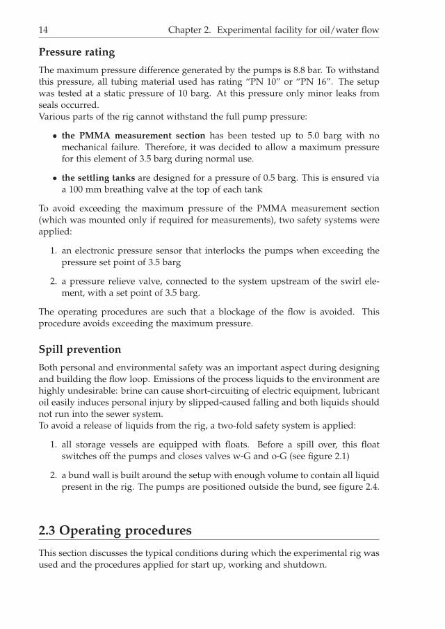
Pressure rating

The maximum pressure difference generated by the pumps is 8.8 bar. To withstandthis pressure, all tubing material used has rating “PN 10” or “PN 16”. The setupwas tested at a static pressure of 10 barg. At this pressure only minor leaks fromseals occurred.Various parts of the rig cannot withstand the full pump pressure:

• the PMMA measurement section has been tested up to 5.0 barg with nomechanical failure. Therefore, it was decided to allow a maximum pressurefor this element of 3.5 barg during normal use.

• the settling tanks are designed for a pressure of 0.5 barg. This is ensured viaa 100 mm breathing valve at the top of each tank

To avoid exceeding the maximum pressure of the PMMA measurement section(which was mounted only if required for measurements), two safety systems wereapplied:

1. an electronic pressure sensor that interlocks the pumps when exceeding thepressure set point of 3.5 barg

2. a pressure relieve valve, connected to the system upstream of the swirl ele-ment, with a set point of 3.5 barg.

The operating procedures are such that a blockage of the flow is avoided. Thisprocedure avoids exceeding the maximum pressure.

Spill prevention

Both personal and environmental safety was an important aspect during designingand building the flow loop. Emissions of the process liquids to the environment arehighly undesirable: brine can cause short-circuiting of electric equipment, lubricantoil easily induces personal injury by slipped-caused falling and both liquids shouldnot run into the sewer system.To avoid a release of liquids from the rig, a two-fold safety system is applied:

1. all storage vessels are equipped with floats. Before a spill over, this floatswitches off the pumps and closes valves w-G and o-G (see figure 2.1)

2. a bund wall is built around the setup with enough volume to contain all liquidpresent in the rig. The pumps are positioned outside the bund, see figure 2.4.

2.3 Operating procedures

This section discusses the typical conditions during which the experimental rig wasused and the procedures applied for start up, working and shutdown.

i

i

“Thesis1” — 2014/1/7 — 18:22 — page 15 — #35i

i

i

i

i

i

2.3. Operating procedures 15

2.3.1 Startup

In case there is no liquid is present in the system, it is filled at a very slow pace.First, valve w-F is closed and o-F opened. The brine pump is regulated to justovercompensate gravity, such that the system is flooded with a few cm/s. Whenthe complete measurement tube is filled, the pump pressure is increased to generatea flow up to 0.5 m/s. At this point, valve w-F is opened and the flow is increasedto almost 1 m/s.Prior to testing, both settling vessels should be completely filled with liquids andthe brine/oil interface should be at an appropriate level. First, the brine level isadjusted by a flow of brine running into both vessels, with their respective controlvalves (valves o-G en w-G in figure 2.1) kept closed until the desired brine level isreached. The next step is flow of pure oil into both vessels to fill them completely,leading to an overflow of oil back into the oil storage vessels via the discharge lining.The oil running through the Coriolis flow meter provides a reference measurementfor the water content of the oil.In all cases a change in pump frequency is performed gradually to avoid excessivepressure changes on the rig.

2.3.2 Operating window

During the tests, the flow rates chosen should be within certain limits. The minimalflow rate that can be measured by both float flow meters is 8.0 m3/h. Lower flowsare possible with respect to the pump, but they will not be detected by the flowmeters downstream of the pumps. The maximum total flow rate depends on theseparating characteristics of the settling tanks, the maximum flow rate for brine(being more than 60 m3/h) and the maximum flow rate for oil (being 35 m3/h, forhigher flow rates, this is the maximum flow rate before air is sucked into the pump;the gravity driven flow from the first oil storage vessel to the second one limits thisprocess). Measurement times are infinite as long as the flow in the measurementtube operates in a water continuous regime. The settling tanks can then deal withthe process streams according to their design specifications (see section 2.2). Inoil-continuous flow not all droplets smaller than 100 µm are separated. Partialseparation in the settling vessels leads to a mixture running through the pumps, inwhich the high shear levels further reduce the droplet size. Experience learned thatoil-continuous tests cannot last longer than approximately 10 minutes.

2.3.3 Shutdown

Before shutting down the system, the oil flow is stopped. Only brine flushes thesystem at an arbitrary flow rate. As soon as all visible traces of oil are removed fromthe system, the flow rate of brine is lowered by decreasing the pump frequency to25 Hz or less. At this lower flow rate, valve w-F is closed, after which the brinepump can be switched off.

i

i

“Thesis1” — 2014/1/7 — 18:22 — page 16 — #36i

i

i

i

i

i


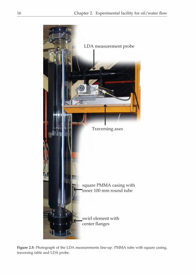
swirl element with center fl anges

square PMMA casing withinner 100 mm round tube

LDA measurement probe

Traversing axes

Figure 2.5: Photograph of the LDA measurements line-up: PMMA tube with square casing,traversing table and LDA probe.

i

i

“Thesis1” — 2014/1/7 — 18:22 — page 17 — #37i

i

i

i

i

i

2.3. Operating procedures 17

swirl element

center fl ange

center fl ange

overpressure sensor

tube connections

fl ow direction

Figure 2.6: Photograph of the swirl element clamped between two tubes, with the two centerflanges in black.

i

i

“Thesis1” — 2014/1/7 — 18:22 — page 18 — #38i

i

i

i

i

i


2.3.4 Maintenance operations

The settling tanks will never provide a perfect phase separation. Even if much lessthan 1% of the phase runs into the wrong storage vessel, over time a significantamount of that phase will build up.

Oil in the water storage vessel The oil layer floats on top of the water. When thewater flow rate is not excessive, this oil remains in this position; the higher viscosityof oil avoids the leak of oil into the water pump.A high hold up of oil in the brine storage vessel is undesirable, it reduces the oilvolume available for tests, and in some occasions, oil can run into the brine pump,for example when the brine level in the storage vessel is low because the brine flowrate being high.This layer is removed by lowering the liquid level below the openings of the waterdischarge lines from the settling tanks. The brine falling into the liquid breaks theoil layer, by which oil chunks are sucked into the brine pump and moved to thesettling tanks. High shear levels in the centrifugal pump should be avoided to min-imize droplet size reduction. For that reason, this procedure should be conductedat a low rotational speed of the pump.

Brine in the oil storage vessel Brine has a larger density than oil and will there-fore settle at the bottom of the vessel. The lower viscosity of brine compared to thatof oil results in an easy suction of brine into the oil pump. For this reason the brinelayer should be kept to a minimum. A submerged pump is located at the bottom ofone oil storage vessel - this continuously removes the lowest liquid layer from thevessel and transfers it directly into the largest settling tank, see figure 2.1.

2.4 Consistency of results

This section discusses the quality of the results - when are the results significantand how do the results reproduce over time.

2.4.1 Reproducibility

Comparability of the oils

Within the research described in this thesis, we used two different oils, indicated byoil A and oil B, see table 2.1. Furthermore, it is known that oil properties changein time due to aging effects. We measured the efficiency of separation for almostthe same conditions at three different moments in time. The distance from swirlelement to pickup tube was 170 cm and the flow rate 56 m3/h.

1. March 8th, 2011, with oil A. The feed droplet sizes were not measured duringthe measurements, but likely to be below 100 µm.

2. March 13th 2012, with oil B. The average feed droplet sizes were measured tobe approximately 80 µm.

i

i

“Thesis1” — 2014/1/7 — 18:22 — page 19 — #39i

i

i

i

i

i

2.4. Consistency of results 19

Table 2.1: Physical properties of model oils used in this thesis.

Quantity Unit Oil A Oil B

Density at 15 C [kg/m3] 869 881

Kinematic viscos-ity at 40 C

[mm2/s] 10 10

Interfacial tensionwith brine at 20 C

[mN/m] 15 26

Constitutionsolvent refined, non-additivated, naftenicmineral oil

solvent refined min-eral oil blended withzinc free additives

3. September 13th 2012, with oil B. The average feed droplet sizes were measuredto be 135 µm.

Figure 2.8 shows a difference in separation efficiency for the three cases. The dif-ferences are significant for the HPO. For the LPO, the measured difference in oilconcentration appears to be smaller than the measurement error. The overall trendis, however, that the efficiency is equal for March 2011 and March 2012, where it islarger for September 2012. The most likely cause for this is the difference in dropletsize in the feed.

Effect of previous tests

The consistency of the measurements has been checked by repeating the same ex-periment in different ways. In figure 2.9 the oil concentrations are shown in theLPO and HPO. The same experiment was performed running from a low oil con-centration in the feed to a high concentration, followed immediately by the reverseorder, i.e. from a high to a low concentration.From these results, no significant difference is noted. In general for the case “highto low”, we observe a higher oil concentration in the LPO. A possible explanationfor that is:

1. longer testing increases the volume of dispersed water in the oil;

2. leading to a higher density of the oil phase;

3. for the same reading of the oil intake, less oil is fed to the system;

4. a lower measured oil concentration in the HPO is interpreted as a higher oilconcentration in the LPO. This effect should be considered when a series oftests is executed. A solution would be to measure the mass flow and densityin the LPO with a Coriolis flow meter, or by measuring the density in the oilfeed line online.

i

i

“Thesis1” — 2014/1/7 — 18:22 — page 20 — #40i

i

i

i

i

i


V01

w-F

level sen

sor

Co

riolis

fl ow

meter

placeh

old

er 2n

d

Co

riolis fl o

w m

eter

tub

e with

sw

irling

fl ow

Q

o-F

Figure 2.7: Photograph of the higher end of the measurement tube, with the actual separationsection, measuring devices and the small settling tank. Labels refer to the scheme in figure2.1

.

i

i

“Thesis1” — 2014/1/7 — 18:22 — page 21 — #41i

i

i

i

i

i

2.4. Consistency of results 21

0.1 0.15 0.2 0.25 0.3 0.35 0.4 0.45 0.5 0.55 0.60

0.1

0.2

0.3

0.4

0.5

0.6

0.7

cin

cou

t

March 2011March 2012September 2012c

out = c

in

Figure 2.8: Oil concentration in the LPO (upper left) and HPO (bottom right). (cout) as func-tion of the oil concentration in the input (cin) for three different days for a measurementsystem of 170 cm at a flow rate of 56 m3/h. Error bars indicate uncertainty in the concen-tration, see appendix C. Feed oil and average droplet size differ. Results obtained with thestrong swirl element.

.

0.1 0.15 0.2 0.25 0.3 0.35 0.4 0.45 0.5

0.1

0.2

0.3

0.4

0.5

0.6

cin

cou

t

low cin

to high cin

high cin

to low cin

cout

= cin

Figure 2.9: Oil concentration in the in- and output for measurement length of 190 cm. Meas-ured in one run from low cin to high cin and vice versa. LPO results are in upper left part,HPO results in lower right part.

i

i

“Thesis1” — 2014/1/7 — 18:22 — page 22 — #42i

i

i

i

i

i


air

oil

emulsion

brine

Figure 2.10: Sample of the “problem” liquids: brine, oil A and emulsion

2.5 Durability of the process liquids

During the tests performed for this research, it was noted that the separability of theprocess liquids changed over time. The interfacial tension decreased significantly,resulting in the formation of a white, viscous layer at the interface of brine and oil(see figure 2.10). When looking at this layer through a microscope, it was found thatit consisted of oil and water droplets - this layer will be called the micro-emulsionlayer. A micro emulsion can only be formed if the interfacial tension between twoliquids is low (a high interfacial tension will prevent the droplet to break up into tothe small sizes required for a micro emulsion) or when the applied shear stress isvery high.The original liquids were acquired in June 2010, the first problems arose in Septem-ber 2011. At that time, the liquid properties were investigated, results are in table2.2. The interfacial tension was measured and found to be less than 1.5 mN/m, afactor 10 smaller than the initial value. The interfacial tension for fresh oil A andfresh brine is 15 mN/m or more. The reduction in interfacial tension must have achemical cause, either a surfactant was added to the system or the liquids changedover time.The viscosity of the degraded oil A was about 20 % higher than that of the originaloil A. This can be caused by the presence of water droplets in the oil. It is at least astrong suggestion that the oil molecules did not become shorter.To understand whether a surfactant is present in the oil or water phase, the inter-facial tension was measured for four different combinations: clean or used brineversus clean or used oil A. All samples were obtained from the bulk liquids, so faraway from the interface layer. From table 2.3 it is clear that a surface active agentmust be present in both phases. Typically, non-ionic surfactants are found in oilwhich can stabilize water-in-oil emulsions, while ionic surfactants are found in thewatery phase which can stabilize oil-in-water emulsions.

i

i

“Thesis1” — 2014/1/7 — 18:22 — page 23 — #43i

i

i

i

i

i

2.5. Durability of the process liquids 23

2.5.1 Possible causes

To identify the surfactant, all possible entry routes for surface active agent(s) to therig were considered. This section describes the different possibilities.

Loading of liquids

If the surface active agent(s) were introduced via the filling process, the effect musthave been noticed from the first tests onwards. This was not the case, making thisentrance route unlikely.

Brine Brine was prepared from tap water and commercially available food gradesalt (NaCl). The tap water lines were used extensively before filling, which shouldhave removed any possible pollution. The salt was doped with anti-caking agent:K4Fe(CN)6, i.e. Potassium Iron cyanide. Since this lacks a non-ionic tail, it is notconsidered as a possible surfactant.

Oil The oil was not analyzed upon delivery, it was assumed that this lubricant oilwas delivered according to specification. A sample was taken and stored. The oilwas transported from the vessels to the rig via hoses provided by Vidol, a trans-porting company. It is not known whether these hoses were clean from surfactants.

Structures in the flow rig

Polymer materials The system is constructed out of polymer materials that mightinteract with the oil. The different materials used are:

• Polypropylene: is not expected to interact with mineral oil

• PVC (Poly Vinyl Chloride): is according to the oil A safety sheet unsuitablefor storage of oil A. Consultation of the oil manufacturer learned that min-eral oil molecules could exchange for plasticizer molecules, making the PVCbrownish and releasing plasticizer into the system. Analysis of oil A from thesetup using the gas chromatogram technique did not show a traceable amountof plasticizer (phthalate). The Infra Red spectrum did not show clear peaksdue to what could be phtalate. Furthermore, mixing clean oil A, clean brineand phtalate together did not result in a micro emulsion.

• PMMA (Poly Methyl MethAcrylate): no interaction with mineral oil in known.

Table 2.2: Physical properties of original and degraded oil A.

Original oil A Degraded oil ADensity (kg/m3) 869 ± 1 870 ± 5Interfacial tensionwith brine(mN/m)

15 ± 1 < 1.5

Viscosity (mPas) 16.6 ± 0.02 20.5 ± 0.03

i

i

“Thesis1” — 2014/1/7 — 18:22 — page 24 — #44i

i

i

i

i

i


Table 2.3: Interfacial tension of the process liquids (mN/m)Clean Brine Degraded brine

Clean oil A 15 ± 1 9 ± 1Degraded oil A 4 ± 2 < 1.5

• EPDM (Ethylene Propylene Diene Monomer): this is a rubber used in theapplied appendages. It is known to be not resistant to mineral oil. The effectof mineral oil is that it diffuses into the rubber, making it grow in volume andloose strength. It is not expected that EPDM molecules get into solution andact as an emulsifier. However, this introduces an uncertainty.

• NBR (Nitrile Butadiene Rubber): a mineral oil resistant rubber, no negativeeffects are expected.

Metal parts The system was manufactured from different parts, containing bothmetal parts (stainless steel AISI 316L) and polymer parts. These parts can containfatty substances on their surface when they are new. The system was only rinsedwith tap water before the oil was added. This means that these fatty substancesmight be dissolved in the oil now. Their effect is unknown.The pump shafts are lubricated using dry PTFE. This means that no lubrication oilcan have leaked from the pumps.The coating of the largest settling tank was replaced because it did not provideenough resistance against corrosion, this has caused different elements to get intouch with the liquids in the setup:

• Coating chunks: Novaguard 840 is a two-component solvent-free phenol/epoxypolyamine coating. It is oil resistant, but can get damaged by brine. Chunksgetting loose and dispersing in the flow are not expected to have an emulsify-ing effect.

• Rust particles: the carbon steel vessel (Fe) corroded to iron oxides (Fe2O3)mainly, which is non-solvable in water or oil. The solid salt is completelypolar, making it not a surfactant.

• Solvents of re-coating: the solvents used for the first recoating step are notpresent in the system. They are very volatile, and would have been noticed inthe Gas Chromatograph analysis (see Appendix A).

In the end, the complete vessel was replaced by a new stainless steel vessel, madeout of 316L steel. Stainless steel is treated after mechanical modifications usinga mordant and a passivating agent. This passivating agent is nitric acid (HNO3)which is ought to remove all mordant and to form a layer of chromium oxide onthe steel. The passivating agent was not actively removed, other then with cold tapwater. However, it was not found in the system, since the pH was almost neutral:6.5.

i

i

“Thesis1” — 2014/1/7 — 18:22 — page 25 — #45i

i

i

i

i

i


Measurement equipment The only electric field present is that of the wire mesh.This has sufficient potential difference to create electrolysis, though that would leadto a high pH by the formation of OH-. The pH of the liquids in the system is 6.5,making this effect negligible.

Contamination from surroundings

Olive oil In the first tests, performed in 2009, some olive oil was added to thesetup to study the behavior of oil droplets in water. The total amount of olive oilinjected in the setup was 0.5 L. The water containing olive oil was removed, andthe parts of the setup that were accessible were mechanically cleaned (being themeasurement tube itself, the storage vessels and the settling tanks) and the rest ofthe setup was extensively rinsed with tap water. There will, however, have remainedsome olive oil residues at the walls.Olive oil is a triglyceride that will decompose into glycerin and oleates. The lattercan act as a surfactant due to their polar head and non-polar tail. To test this, a batchof olive oil was completely decomposed by adding NaOH, which was added in ahigher concentration than present in the setup to a clean oil A/Brine system. Fromthis test it was concluded that this soap could not account for the dense emulsionobserved in the test rig.

Bacteria Mineral oil contains energy bacteria might use to live. The excreta pro-duced by the bacteria can act as an emulsifier. Two tests were carried out to findbacteria:

• Saybolt performed a standard test, in which they grew the bacteria on stand-ard soils. No bacteria were found for these soils.

• Since the conditions in the Delft test rig are extreme for bacteria (being verysalty), also non-standard bacteria could be present. Some samples were there-fore also investigated optically using phase contrast microscopes. This wasdone with the very kind help of dr. L. Robertson of TU Delft. There weresome bacteria present, but there was definitely no flourishing bacteria colony.Figure 2.11 shows a single bacteria which we found after extensive searching.

Human error In case somebody deliberately wanted to frustrate our research, heor she could have added detergent to the system. Many detergents foam, where nofoaming was observed. Some ionic surfactants (like SDS) have a low solubility inwater with a high salt content. No solids have been observed in the water phase.

Suction of other substances The system sometimes contains regions with a lowerpressure than the surroundings. The set-up is, however, constructed in such a waythat the only surrounding substance is air. It is therefore highly unlikely that asurfactant was sucked into the system. From the surroundings, aerosols, dust andmaybe insects might fall into the setup.

i

i

“Thesis1” — 2014/1/7 — 18:22 — page 26 — #46i

i

i

i

i

i


Figure 2.11: Microscope image of the oil layer. In the upper right corner, inside the red circle,there is a small black spot that might be a bacteria, bacteria show dark in the photograph.Scale is unkown.

Oxidation due to air The system is in contact with air: all the vessels are madebreathing and during operation, the overflowing outlets of the settling tanks alsointroduce intense mixing of the oil and air. It is known from the Material SafetyData Sheet (MSDS) of oil A that the contact with strong oxidizing agents should beavoided - being a hint that oil A can oxidize.The oxidation process will create =O groups on the long chains, which will createthe possibility of forming polar bonds with other molecules. These polar bindingswill increase the mixing with water and may be accounting for the lower interfacialtension.An infrared transmittance spectrum was made of the oil. Infra red light with awavelength of 174 · 103 m−1 is strongly absorbed by the “=O” group, which ispresent in oxidized oil. The results are presented in figure 2.13. Based on theseresults, no significant amount of oxidized oil is found.

Conclusion

No clear reason for the decrease in interfacial tension was uncovered. To continuemeasurements all process liquids were replaced after having cleaned the rig thor-oughly. Since the original oil (oil A) was not available anymore, the oil which closestresembles oil A was chosen: oil B. The physical properties of the different oils areprovided in table 2.1 - all results presented in this thesis concern oil B, unless oth-erwise indicated.The quality of oil B was tested over time for its interfacial tension. A decreasein interfacial tension would result in a lower separation efficiency. The interfacialtension was determined with a Krüss Easydrop, a contact angle microscope. Waterdispersed in the oil was removed in a centrifuge before measurements, since atransparent oil phase is required. Figure 2.14 shows the results over time. Nodecreasing trend for the interfacial tension is observed.

i

i

“Thesis1” — 2014/1/7 — 18:22 — page 27 — #47i

i

i

i

i

i


(a) Scheme

(b) Overview picture

(c) Detail picture

Figure 2.12: Test facility for the tests with the cyclone with rotating swirl generator.

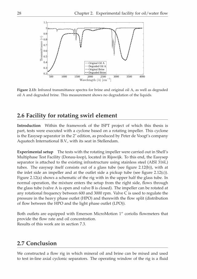
i

i

“Thesis1” — 2014/1/7 — 18:22 — page 28 — #48i

i

i

i

i

i


500 1000 1500 2000 2500 3000 3500 40000.2

0.3

0.4

0.5

0.6

0.7

0.8

0.9

1

1.1

Wavelength (λ) [cm−1

]

Tra

nsm

itta

nce

(τ)

Original Oil A

Degraded Oil A

Original Brine

Degraded Brine

Figure 2.13: Infrared transmittance spectra for brine and original oil A, as well as degradedoil A and degraded brine. This measurement shows no degradation of the liquids.

2.6 Facility for rotating swirl element

Introduction Within the framework of the ISPT project of which this thesis ispart, tests were executed with a cyclone based on a rotating impeller. This cycloneis the Easysep separator in the 2" edition, as produced by Peter de Voogt’s companyAquatech International B.V., with its seat in Stellendam.

Experimental setup The tests with the rotating impeller were carried out in Shell’sMultiphase Test Facility (Donau-loop), located in Rijswijk. To this end, the Easysepseparator is attached to the existing infrastructure using stainless steel (AISI 316L)tubes. The easysep itself consists out of a glass tube (see figure 2.12(b)), with atthe inlet side an impeller and at the outlet side a pickup tube (see figure 2.12(c)).Figure 2.12(a) shows a schematic of the rig with in the upper half the glass tube. Innormal operation, the mixture enters the setup from the right side, flows throughthe glass tube (valve A is open and valve B is closed). The impeller can be rotated atany rotational frequency between 600 and 3000 rpm. Valve C is used to regulate thepressure in the heavy phase outlet (HPO) and therewith the flow split (distributionof flow between the HPO and the light phase outlet (LPO)).

Both outlets are equipped with Emerson MicroMotion 1“ coriolis flowmeters thatprovide the flow rate and oil concentration.Results of this work are in section 7.3.

2.7 Conclusion

We constructed a flow rig in which mineral oil and brine can be mixed and usedto test in-line axial cyclonic separators. The operating window of the rig is a fluid

i

i

“Thesis1” — 2014/1/7 — 18:22 — page 29 — #49i

i

i

i

i

i

2.7. Conclusion 29

50 100 150 200 250 300 3500

10

20

30

40

50

age (days)

σ (m

N/m

)

Figure 2.14: Interfacial tension of oil B and demineralized water. Age is relative to the fillingof the rig with this oil

.

flow between 10 and 60 m3/h. The oil concentration in the mixture can be chosenas any value between 0.10 and 0.90.Some bottlenecks in the rig hold back the optimal performance, for future work,one could consider taking the following measures:

• Inlet flow meters: the current float flow meters have a large measurementerror, provide slow readings and are sensitive to density changes in the liquid,which are likely to occur for the oil phase during a measurement day; a betteralternative is:

• LPO flow meter: a direct measurement of the density in the LPO, combinedwith the mass flow rate, reduces the accuracy of separation efficiency meas-urements to a great extend. Considering the mass balance, this extra Coriolisflow meter makes the inflow flow meters over complete, since the inflow canbe computed from the outflow.

• Rig alignment: the measurement section is constructed out of PVC tubes andappendages. The limited stiffness of this material prevents a perfect axialalignment;

• Storage vessel positioning: the current position of the outflow openings ofthe storage vessels (15 cm above their bottom) is not convenient during main-tenance operations: the tanks can not be fully drained by gravity, the last bitshould be removed manually. The remaining liquid volume also introducesan operational problem since a floating oil layer in the brine storage vesselsslips easily into the pumps, and the oil storage vessels suffer from water hol-dup at the bottom. It is suggested to move the outflow to the ground plane ofthe tanks to minimize the pollution of the brine feed with oil and vice versa.

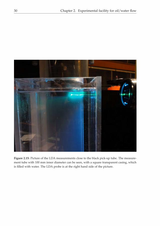
i

i

“Thesis1” — 2014/1/7 — 18:22 — page 30 — #50i

i

i

i

i

i


Figure 2.15: Picture of the LDA measurements close to the black pick-up tube. The measure-ment tube with 100 mm inner diameter can be seen, with a square transparent casing, whichis filled with water. The LDA probe is at the right hand side of the picture.

i

i

“Thesis1” — 2014/1/7 — 18:22 — page 31 — #51i

i

i

i

i

i

CHAPTER 3

Experimental methods

Where the previous chapter focussed on the flow rig in which the tests took place,explains this chapter all measurement methods used for the work in this thesis.Section 3.1 introduces Laser Doppler Anemometry, section 3.2 briefly explains thenumerical methods used for fluid flow calculations. Separation efficiency is an im-portant qualification of a separation device and the followed measurement strategyis introduced in section 3.3. Droplet sizes are measured using the direct photo-graphy method in section 3.4. A new capacity based wire-mesh technique in section3.5 is applied for phase distribution measurements.

3.1 Laser Doppler Anemometry

There are various ways to measure velocities inside transparent fluid flows. In caseof LDA, the Doppler-shift in the frequency of the light reflected from a particle isused to measure the particle velocity. This velocity -under appropriate conditions-is a measure for the fluid velocity. LDA is since its introduction in the 1980’s acommon technique in fluid dynamics research.It is not within the scope of this thesis to explain the mechanism of LDA extensively.For an introduction in LDA and more background information, please see Durstet al. [18] or Tummers [19].

3.1.1 LDA apparatus

The fluid flow is examined using a 2D-Laser Doppler Anemometry (LDA) operatedin back-scatter mode. The laser beams enter the experimental setup via a PMMAsquare water-filled box surrounding the tube (see figure 2.5). This box reducesthe refraction of laser light at the tube wall. To reduce remaining refractive effectsmeasurements are only done along the line perpendicular to the box surroundingthe tube and through the center of the tube. Durst et al. [18] describe the measure-ment principle of LDA.The light from a 4W Argon laser is split into two 488.0 nm beams for the axial

31

i

i

“Thesis1” — 2014/1/7 — 18:22 — page 32 — #52i

i

i

i

i

i

32 Chapter 3. Experimental methods

velocity and two 514.5 nm beams for the azimuthal velocity. For both colors onebeam is shifted with 80 MHz to obtain a direction ambiguity. The beams are focusedwith a 132.0 mm lens, resulting in a measurement volume of 0.2 mm in the radialdirection and 0.03 mm in the azimuthal and axial direction. The burst correlation isconducted in a Dantec F60 BSA signal processor.The average velocity is calculated using an in-house developed software package,see Belt [20]. The following filter actions are performed: (i) removal of data pointswith a value more than 5 times the standard deviation from the average value; (ii)samples obtained from the same tracer particle by introduction of a dead time;(iii) velocity bias by overestimation of fast tracer particles is corrected using a2D+weighing scheme as introduced by Tummers [19].

3.1.2 Measurement volume

The measurement volume is created at the point of intersection of two laser beams.Due to a Gaussian distribution of the intensity inside a laser beam, the measure-ment volume itself is ellipsoidal shaped, with a geometry as given in Figure 3.1.According to Adrian [21], the dimensions of the measurement volume in x-, y- andz-direction can be expressed as:

dm =de−2

cos (κ)(3.1)

lm =de−2

sin (κ)(3.2)

hm = de−2 (3.3)

respectively, with κ being half of the angle between the incident laser beams andde−2 the diameter of the focused laser beam, which can be expressed as

de−2 ≃ 4 f λm

πDe−2(3.4)

where λm is the wavelength inside the medium and f the focal length of the lens.From equation 3.4 it can be seen that for small measurement volumes, either largeincoming beam diameters are required or short focal lengths.The TSI 9832 probe, with a diameter of 83 mm, has all optical components integ-rated to perform backscatter LDA. Each beam pair is emitted with an inter-beamdistance of 50 mm and the different pairs are placed orthogonally. The beams arefocused using a 132.0 mm lens. The blue light is used for the axial velocity, thegreen light for the azimuthal velocity, this due to the higher sampling frequency ofthe green beam pair.The diameter of the laser beams has been determined to be 3.0 mm. The dimensionsof the measurement volume are given in Table 3.1.

3.1.3 Tracer particles

With LDA, the velocity of the tracer particles is determined, not of the fluid itself.Therefore, the choice of the particles is very important for an accurate determination

i

i

“Thesis1” — 2014/1/7 — 18:22 — page 33 — #53i

i

i

i

i

i

3.1. Laser Doppler Anemometry 33

Table 3.1: Measurement volumes in water for the used setup, according to Equation 3.1.

λ dm (µm) lm (mm) hm (µm)488.0 27.6 0.205 27.3514.5 29.1 0.216 28.8

of the fluid flow.Various requirements for the particles need to be full filled:

• The particles must be small enough and its density close enough to make theparticle naturally buoyant in order to follow the smallest vortices in the flow.This smallest scale is in the order of the Kolmogorov micro scale.

• Presence of the particles should not influence the fluid, nor dynamically, norchemically.

• Particles should have a high reflectivity for the incident light.

• The particles must be naturally buoyant to avoid a bias in the vertical direc-tion.

As a practical implementation of the requirements above, hollow glass spheres area very suitable choice, which are cheap as well.The ability of the particles to follow the flow, is mostly dependent on their densitydifference with the liquid and their size. Particle motion is determined by drag,buoyancy, gravity, lift and virtual mass forces. The Lagrangian motion of a rigid,spherical particle of diameter d and density ρp in a viscous flow can be describedby the Basset-Boussinesq-Oseen (BBO) equation [19]. A simplified version of thisequation can be used for seeding particles

π

6d3ρp

dvp

dt= −3πµd(vp − v f ) (3.5)

where lift, gravity, virtual mass and buoyancy forces are neglected. The left-handside of 3.5 is the acceleration force, the right-hand sight represents Stokes’ drag.Another way to describe the ability of the particles to follow the flow, is by express-ing their motion in Fourier components. As long as their maximum frequency ishigher than the fluids highest frequency, the particles can track the smallest flowstructures. The flow frequency is given by ω = 2π fturb. By using the substitutionproposed by Tummers [19], v f = eiωt and vp = η(ω)eiωt the amplitude ratio, |η|,can be expressed as

|η(ω)| =Ω√

Ω2 + ω2where Ω =

18ν

σrd2p

, (3.6)

with σr the density ratio ρp/ρ f . The amplitude ratio is a measure of the particlessensitivity to follow changes in fluid flow. It can be seen from equation 3.6 that forvery high frequencies the amplitude ration η becomes negligible and therefore theparticles are not very sensitive to the fluids motion.

i

i

“Thesis1” — 2014/1/7 — 18:22 — page 34 — #54i

i

i

i

i

i


Figure 3.1: Geometry of the measurement volume for LDA. Two incident laser beams fromthe left are converged by a lens into the measurement volume.

To obtain a sufficient temporal resolution to capture the smallest flow structures,at the Kolmogorov microscale, enough particles should cross the measurementvolume. As a criterion for the minimum sampling rate, Durst et al. [18] mention aminimal sampling frequency of 2 fturb. Because particles are distributed randomlyin the fluid, particle arrivals at the control volume are not equally distributed intime. To ensure enough samples during moments of high velocity fluctuations aswell, the average particle arrival frequency should be larger than 2 fturb to meet theminimum condition.

In this work, we used two kinds of seeding particles:

1. neutrally buoyant glass spheres with a diameter with an average of 8 µm -these were used until multiphase experiments started. During the experi-ments with both oil and water, no seeding particles were present;

2. remaining small oil droplets and solids in the flow - these were used whenthe liquids in the system were used for oil/water experiments as well. Oildroplets with a diameter in the order of µm are very stable and have a highreflection efficiency.

3.1.4 Traversing system

The probe is mounted on a digital driven traversing system, such that the meas-urement volume covers the complete cross-section of the test section. The probetraverses along the vertical axis, i.e. in axial direction. The measurement tubeis surrounded with a square PMMA box filled with water. The entrance of lightthrough a flat surface reduces refraction.Due to refraction, displacement of the probe will not correspond to the displace-ment of the measurement volume. The refractive index of water, nw is higher thanthat of air na, changing the angle of the incident beam in the measurement volume.

i

i

“Thesis1” — 2014/1/7 — 18:22 — page 35 — #55i

i

i

i

i

i

3.2. Numerical method 35

The correction factor between the movement of the probe and the movement of themeasurement volume, is given by:

CL =tan(α)

tan(

arcsin(

nanw

sin(α))) (3.7)

where α is given by arctan(

D/2L

), with D the distance between the incoming laser

beams and L the focal length of the lens.Other refractive changes might be occurring, but since these are much smaller andmore difficult to correct for, for the time being, they will be neglected.

3.1.5 Void kernel

During measurements, the center of the tube contained a region that was non-transparent, resembling an air or void kernel. This prevented the laser beams toreach the center of the pipe. The high pressure difference in radial direction causedby the centrifugal acceleration can make the water cavitate or result in dissolvedgases coming out of solution. The pressure difference ∆p between the center andthe wall is estimated by

∆p =∫ R

0

ρvθ(r)2

rdr, (3.8)

with ρ the liquid density and vθ(r) the azimuthal velocity at position r. For a typicalcase that will be discussed in section 4.4 (figure 4.8(a)) ∆p = 1.9 bar. The pressure asmeasured at the wall was about 1.6 bar. A quick and dirty estimation suggests thepressure in the center of the tube to be negative. Most likely, enough gas escapes theliquid phase to build up a vapour kernel. A quantitative description of the pressurein this kernel is not produced in this work. Since the size of the void kernel was notconstant over subsequent measurement series, not all measurement sets run to thesame radial position.Numerical results do not show a vapor kernel, for which various reasons can begiven. First, the pressure difference between the wall and center is 1.05 bar. Thislower value results from lower azimuthal velocities for r < 35 mm (see figure 4.8(a)).Furthermore, the numerical method does not incorporate two-phase-flow effects;even with negative pressure, the numerical approach assumes that the phase re-mains liquid. The continuous presence of liquid water with accompanying shearforces changes the flow pattern significantly compared to the experimental casewith a void at the center of the tube.

3.2 Numerical method

The work described in this thesis is part of an ISPT project, which covers both exper-imental and numerical work on an in-line axial cyclone for liquid-liquid separation.The presented results further on are compared with numerical work of Slot [13].This section gives a brief overview of the applied method.

i

i

“Thesis1” — 2014/1/7 — 18:22 — page 36 — #56i

i

i

i

i

i


3.2.1 Single Phase

The flow field is resolved by solving the Reynolds averaged Navier-Stokes equationsfor transient incompressible turbulent flow using the commercial package AnsysCFX 14.0. Reynolds stresses are modelled using the Reynolds Stress Model (RSM)implementation SSG. The typical computational domain consists out of 2.3 millionhexahedral elements.The boundary conditions applied are:

• Inlet: axial velocity uz,b, density ρ and viscosity µ.

• HPO: pressure pHPO

• LPO: mass flow rate dmLPO/dt.

All simulations were performed for a time-dependent flow. The presented resultsare time-averaged flow solutions.

3.2.2 Two Phase Flow

For multi-phase flow, the problem is treated according to both the Euler-Lagrangianand Euler-Euler model. In the Euler-Lagrangian approach, the single phase solutionfor water is taken as the continuous phase velocity profile. In this work, the path ofmany droplets is computed based on the continuous phase time-averaged solutionwith a CFX implementation of turbulent dispersion. There is no coupling from thedroplets motion towards the continuous phase velocity.

In the Euler-Euler model both phases (oil: o and water: w) are defined as continu-ous, interpenetrating fluids. In the formulation of the drag, however, the water isdefined as continuous and the oil as dispersed with droplets of a certain diameter.For each computational cell in the setup, the following parameters are monitored:volumetric oil fraction, average velocity for both phases separately and the dropletsize distribution (in discrete bins). Individual droplets are not considered in thisapproach. During the computation, based on drag laws for ensembles of disperseddroplets and the velocity difference between the phases, the drag, breakup andcoalescence are calculated per cell.The Euler-Euler method requires extensive models to accurately describe the dragbetween the phases and the consequences for the droplet size distribution.The boundary conditions applied are:

• Inlet: axial velocity uz,b, volumetric oil fraction α, droplet diameter D, densit-ies ρo and ρw and viscosities µo and µw.

• HPO: pressure pHPO

• LPO: axial bulk velocity uz,LPO.

i

i

“Thesis1” — 2014/1/7 — 18:22 — page 37 — #57i

i

i

i

i

i

3.3. Efficiency measurements 37

3.3 Efficiency measurements

There are various methods to express the separation efficiency of a cyclone. We willuse three methods in this thesis. The first method is by calculating the fraction ofthe oil which runs into the LPO, the so-called dilute efficiency:

ηdilute =Φoil, LPO

Φoil, in, (3.9)

this measure is a good qualification if the objective is to remove oil from the waterstream.The second efficiency considers the total amount of dispersed phase running intothe ‘wrong’ outlet: it is the volumetric oil flow in the HPO plus the volumetric waterflow in the LPO. This results in:

ηdispersed = 1 − Φwater in LPO + Φoil in HPOΦtot

(3.10)

The final efficiency measure, we call the bulk efficiency. The advantage over thedispersed and dilute efficiency is that its range is from 0 to 1: if the oil concentrationin the outputs is equal to that of the input, the bulk efficiency is 0, if there is onlyoil in the LPO and water in the HPO, it is 1:

ηbulk =12

(cin − cHPO

cin+

cLPO − cin

1 − cin

). (3.11)

An evaluation of the uncertainty in the calculated oil concentration can be found inAppendix C.

3.4 Droplet sizing

The size of the droplets is a very important parameter for the use and design ofliquid-liquid cyclones. Measuring the droplet size distribution has been topic ofextensive research. Bae and Tavlarides [22] give an extensive overview of possiblemeasurement principles. Not all of these techniques are capable of dealing withhigh (> 1%) dispersed volume fractions. The following methods are feasible: directphotography, light scattering, chemical reaction, drop stabilization and scintilla-tion. Direct photography is the standard method for calibration of other methods[23] and should be conducted in-situ, e.g. with an intrusive endoscope. Alternativetechniques, like a laser scattering method discussed by Desnoyer et al. [24], tradi-tionally required tapping of liquids to a by-pass for dilution. Nowadays, intrusivelaser-scattering based methods are available. According to a review by Maaß et al.[23], none of them prove to deliver results with a quality comparable to the resultsof direct photography.

i

i

“Thesis1” — 2014/1/7 — 18:22 — page 38 — #58i

i

i

i

i

i


In this work, we use two different ways of droplet sizing: (i) direct photographywith an endoscope system (section 3.4.1)and (ii) laser-scattering in an off-line man-ner (section 3.4.2). A third method using glass fibre probes (section 3.4.3) has beenassessed, but not used. Direct photography proved to be the most precise, thoughelaborate [23]. The second method should be more efficient in execution.

3.4.1 Direct photography with an endoscope

The droplets inside the test rig are photographed via an endoscope configuration(see figures 3.2(a) and 3.2(b)). This consists of a 10 mm thick stainless steel tubewith a lens at both sides. The distance between the lenses is adjustable to enablefocussing.The endoscope is mounted in the measurement tube orthogonal to the wall as infigure 3.2(b). From the opposite side, a light guide is inserted, such that light isemitted towards the endoscope. The position of the light-guide, and therewith thedistance between the tip of the endoscope and the light-guide, is adjustable. Thelight-guide is illuminated with an adjustable halogen lamp, Schott 2500 LCD, whichemits up to 1300 lumen in a spot with 5 mm diameter.Images are captured using a high speed camera. Two different cameras were used:

• An IDT Motion Pro Y4

• An Olympus i-SPEED 2

Both cameras were used in combination with a 75 mm adjustable lens. The proced-ure for adjustment of the lighting and lens setting was such that optimal lightingconditions were obtained. First, the light guide was set to touch the endoscope lens.The focus of the lens on the camera was adjusted to provide sharp images of thefibers in the light guide. The light guide was then gradually pulled out, until therewas just enough light to discriminate droplets at the selected shutter speed. Thisprocedure resulted in a focal plane just ahead of the endoscope lens. The distancebetween the endoscope and light guide was not constant for all measurements.The magnification of the camera system is determined by measuring the diameterin pixels of the light guide - this is done when the measurement section is filledwith transparent brine. This scale is used to size the pictured droplets.

Influence of the endoscope

The endoscope is an intrusive measurement technique. The diameter of the endo-scope is very significant compared to the tube diameter (10 mm vs 100 mm). Toaddress the influence of the endoscope and light guide on the flow, two tests wereperformed. First, the single phase fluid velocity was measured using Laser DopplerAnemometry and secondly, the separation performance was measured with andwithout the endoscope.

Velocity profile Figure 3.3 demonstrates the influence of the presence of the en-doscope on the fluid velocity. The most significant difference is the reversal of theaxial velocity around the center of the tube, for a complete insertion, the velocity

i

i

“Thesis1” — 2014/1/7 — 18:22 — page 39 — #59i

i

i

i

i

i

3.4. Droplet sizing 39

is pointed upward on the axis - for the other two cases and the situation withoutendoscope, it points downward.

Efficiency The efficiency of separation was measured with and without the en-doscope, according to the method introduced in section 3.3. Figure 3.4 points outthat with the endoscope inserted into the measurement tube, the phase separationis reduced by roughly a factor of 2. This is most likely caused by a distortion ofthe flow in the center region, where an oil kernel should be formed. From the LDAresults (figure 3.3(b) we already understood the strong effect on the center region.When the presumed oil kernel is breaks up, mixing occurs, which reduces the phaseseparation.The effect on the measured droplet distribution cannot be determined experiment-ally. It is expected that it is unlikely that droplet break-up occurs at the endoscopeitself - the break-up event should then be captured by the camera. Changing flowpatterns, however, will make it impossible to relate the measurement location anddroplet size to the undisturbed situation.

Image processing

The obtained images contain the droplet size information. Although a human eyerecognizes the droplet shapes, it is not straightforward to automate the recognitionand therewith conversion of images to droplet size distributions. The following,manual, procedure was followed to obtain statistical information from the dropletimages:

1. Recorded images (fig. 3.5(a)) are optimized using the “autotone” and “auto-contrast” features of Adobe’s Photoshop (fig. 3.5(b)).

2. Manually circles are drawn over droplets using ImageJ, about 300-400 for eachcase. Due to the manual fit, some circles will be too large, others too small.We assume that this effect averages out.

3. The area of the droplets in pixels is converted to the diameter, according to

D = 2√

A (pixels)

πlengthpixel

4. The droplet diameters are distributed in bins with given droplet size intervals.

5. The number of droplets per bin is smoothed using a moving average over a 5bin interval.

6. Using MATLAB, the following Gaussian function is fitted for the smootheddistribution:

f (x) = a1e

(x−b1

c1

)2

+ a2e

(x−b2

c2

)2

+ a3e

(x−b3

c3

)2

(3.12)

(fig. 3.5(c)).

7. The resulting fitted curve represents the distribution of the number of dropletsfor given size. This is transformed to the volume occupied by the given sizeaccording to the relation ( fv(D) = 1/6πD3 f (D))

i

i

“Thesis1” — 2014/1/7 — 18:22 — page 40 — #60i

i

i

i

i

i


halogen lamp

glass fi bre light guide

endoscopehigh speed camera

measurement tube

(a) Photograph of the equipment used for direct photography of droplets inside the measurement tube.

endoscope

10 cm

~ mm10 mm6 mm

(b) Schematic drawing of the placement of the endoscope in the tube. Light-guide and Endo-scope are aligned.

Figure 3.2: Schematic and photograph of the equipment used for the direct droplet photo-graphy measurements.

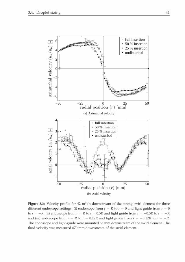
i

i

“Thesis1” — 2014/1/7 — 18:22 — page 41 — #61i

i

i

i

i

i


−50 −25 0 25 50

−6

−4

−2

0

2

4

6

radial position (r) [mm]

azim

uth

alve

loci

ty(u

θ/u

b)

[-]

full insertion

50 % insertion

25 % insertion

undisturbed

(a) Azimuthal velocity

−50 −25 0 25 50

−1

0

1

2

3

4


axia

lve

loci

ty(u

z/u

b)

[-]

full insertion

50 % insertion

25 % insertion

undisturbed

(b) Axial velocity

Figure 3.3: Velocity profile for 42 m3/h downstream of the strong-swirl element for threedifferent endoscope settings: (i) endoscope from r = R to r = 0 and light guide from r = 0to r = −R, (ii) endoscope from r = R to r = 0.5R and light guide from r = −0.5R to r = −R

and (iii) endoscope from r = R to r = 0.12R and light guide from r = −0.12R to r = −R.The endoscope and light-guide were mounted 55 mm downstream of the swirl element. Thefluid velocity was measured 670 mm downstream of the swirl element.

i

i

“Thesis1” — 2014/1/7 — 18:22 — page 42 — #62i

i

i

i

i

i


0.2 0.25 0.3 0.35 0.4 0.45 0.5 0.55 0.6

0.1

0.2

0.3

0.4

0.5

0.6

0.7

0.8

cin

cout

full endoscope insertionno endoscope

Figure 3.4: Comparison of the oil concentration in LPO (upper left) and HPO (lower right),with and without endoscope present. Strong-swirl element, 170 cm length and 50 mm pickuptube diameter.

3.4.2 Liquid sampling and off-line analysis

As an alternative to the in-situ investigation of the droplet size distribution, testswere also done with off-line analysis in a device based on laser diffraction: a Beck-man Coulter LS 230. The procedure to obtain a droplet size distribution exists ofthree parts (i) liquid tapping (ii) liquid conservation and (iii) feeding into the laserdiffraction apparatus.

Mechanism During the 1970s, several authors suggested the possibility to use theforward scattering of coherent light to deduce the particle size distribution [25].Based on this work, different devices were brought to market like Malvern In-struments and Coulter. These devices first used only the Fraunhofer diffractionapproximation, however, nowadays these methods also include the full Mie scatter-ing theory, being the complete solution of Maxwell’s equations for the scattering ofelectromagnetic radiation by a sphere.According to Syvitsky [25], the scattering by spheres of radius a at small angle θ isreasonably equal to the diffraction by apertures of the same diameter:

I(θ) = a4C

[J21 (kaθ)

(kaθ)2

], (3.13)

with λ the wavelength of light, k = 2π/λ, C a constant and J1 the first order Besselfunction of the first kind.For a range of particle sizes n(a), the intensity pattern changes to:

I(θ) =∫

n(a)a4

[J21 (kaθ)

(kaθ)2

]da. (3.14)

The aim of the laser-diffraction sizing method is to obtain a measure for n(a), which

i

i

“Thesis1” — 2014/1/7 — 18:22 — page 43 — #63i

i

i

i

i

i


means to invert equation 3.14. The equation cannot be inverted in a straight-forwardway. Syvitsky [25] provides an overview of the different solution techniques. Thecommercially available devices have these solution techniques implemented, suchthat they estimate the particle size distribution n(a) based on the measured lightpattern. The output of a laser-diffraction based device consists of an estimation ofthe droplet size distribution.

Sample requirement The oil/water mixture which is fed to the cyclone investig-ated in this thesis has a high droplet density which scatters the light uniformly (themixture is opaque). This opaqueness prevents the determination of the droplet sizedistribution and can be resolved by tapping liquid, dilution and subsequent off-lineanalysis. The required liquid loading is device dependent. For the Beckman-CoulterLS 230 used in this research, at maximum of 10 % of incident light may be scatteredto provide a successful measurement.

Liquid tapping Liquid is removed from the flow rig using a stainless steel tube.This tube has a diameter in the order of mm’s, while the tube from which the liquidis sampled is 100 mm wide. See figure 3.6 for a scheme. The small tube is insertedperpendicularly to the flow rig, such that its depth of penetration in the tube canbe adjusted. The inlet of the tube is bent, such that its opening points towards theupstream direction of the flow.From tests with the endoscope (see figure 3.3) we know that the insertion of a rodin the swirling flow region severely effects the flow pattern in the tube. These testswere not repeated for the tube we used for liquid tapping, but the basic effect islikely to be very similar. We do therefore not know whether the tapped liquidoriginates exactly from the tapping location in absence of the tapping tube.In an ideal situation, the velocity at the positions far upstream (1), just upstream (2)and in the sampling tube (3) as indicated in figure 3.6 is equal. We do, however, notimpose an under pressure at the outlet of the tube and therefore the fluid velocityin the tube at location (3) is significantly lower than at (1).Two effects can be distinguished that affect the droplets entering the sampling tube:

1. the obstacle imposed by the sampling tube diverts some of the liquid from itsotherwise undisturbed trajectory. Due to inertia, smaller droplets will followthe stream lines more easily, leading towards a bias to sample large droplets;

2. the diameter of the sampling tube is smaller than that of the swirl tube, whichleads to a lower Reynolds number (∼ 106 outside and ∼ 104 inside). Viscouseffects apply a larger shear force on the droplets, tearing them apart. Thisleads to an under prediction of the droplet size;

3. the Reynolds number is lower inside the pickup tube. The lower turbulenceleads to an increase in the size of the smallest eddies, which will lead toreduced droplet breakup. This follows from Hinze’s theory that will be in-troduced in section 6.1.1. From this reasoning, the flow in the small tubepromotes coalescence and will bias the end result towards larger droplets

The order of magnitude of these three effects has not been determined during thepresent research. Effect 1 can be avoided by actively controlling the velocity in the

i

i

“Thesis1” — 2014/1/7 — 18:22 — page 44 — #64i

i

i

i

i

i


sampling tube with the aid of a vacuum system. Since effects 2 and 3 cannot bemitigated, we did not put effort in an expensive, controllable vacuum system.

(a) Original photograph, due to the lowcontrast no droplets can be seen

(b) Same photograph with enhanced con-trast

0 100 200 300 400 500 6000

0.02

0.04

0.06

0.08

0.1

0.12

0.14

0.16

Droplet size (Dd) [µm]

rela

tive

occ

ure

nce

Original data

Averaged data

Fit

(c) Counted, averaged and fitted fractions of droplet size bins. Averagingprocedure was a moving average over 5 bins, fitting to a lognormal distri-bution.

Figure 3.5: Illustration of the process used for the estimation of droplet size distributionsbased on direct droplet photography.

Emulsion conservation The tapped liquid is collected in a beaker. The stationaryliquid settles due to gravity, destroying the droplets. To conserve the droplets, thebeaker contains a solution of 50 g/l BRIJ-35, which is proven to prevent dropletcoalescence (see Gunning et al. [26] and Hibberd et al. [27]) and be unaffected bysalt (see Mapstone [28]). BRIJ-35 is a non-ionic surfactant with normal solubilityfor brine compared to water. During tests conducted in the present research, weconfirmed the stabilizing effect of BRIJ-35 on the liquids used. This was done bymeasuring the droplet size in the same sample at different times after obtaining thesample. Up to 2 hours of rest, no changes in the measured droplet size distributionswere observed.

i

i

“Thesis1” — 2014/1/7 — 18:22 — page 45 — #65i

i

i

i

i

i


100 mm

6 mm

4 mm

1

2

3

sampling tube

measurement tube

Figure 3.6: Schematic of liquid tapping in the test tube. Three points are indicated: 1.upstream, far from the tube, 2. just upstream the sampling tube and 3. inside the samplingtube.

Dilution and insertion The actual measurement is performed in a Beckman CoulterLS 230. According to the manual, the system is prepared with tap water for back-ground measurements. The sample is added using a pipette until the required lightattenuation is obtained.The liquid is circulated through the measurement chamber with a pump. Thispump is likely to break up droplets due to shear. This effect was determined exper-imentally, see figure 3.7: the measured droplet size gets smaller when the sampleresides longer in the Coulter.

3.4.3 Glass fiber sensor

Glass fibres form a common technique for both size and velocity measurement ofdispersed droplets. Harteveld [29] extensively investigated glass fiber probes ingas/liquid systems. In principle, the same method can be applied to other mul-tiphase flow systems. This section investigates the possibility of the use of glassfiber probes inside the oil/water system of an axial cyclone.

Device A typical glass fiber probe sensor consists of four glass fibres: three ina triangular configuration, the fourth somewhat larger fibre in the middle of theothers. The glass fibres face upstream and their extremities are sharpened. Figure3.8 provides a top and side view of the sensor.

Measurement principle Light is fed to each glass fiber, which is emitted into theliquid at the tip. Reflected light is collected through the same glass fiber. A Y-splitter is used to separate the incident and reflected light, after which the intensityof the reflected light is recorded. The transmission of light depends on the refractiveindex of the liquid surrounding the tip. Typically, glass has a refractive index in theorder of 1.5, oil also about 1.5 and water 1.3. When present water will therefore

i

i

“Thesis1” — 2014/1/7 — 18:22 — page 46 — #66i

i

i

i

i

i


20001000100101

Particle Diameter (µm)

14

12

10

8

6

4

2

0

Volu

me

(%)

0 min

2 min

10 min

6 min

8 min

4 min

Figure 3.7: Droplet size distribution as measured with the Beckman Coulter LS230. The samesample was analyzed at the indicated times.

reflect more light than oil. When a liquid-liquid interface is present close to the tip,more light will be reflected into the glass fiber. In conclusion, the obtained signalcontains information on the phase in which the tip is submerged and the presenceand type of interface close to the tip.

Measurements of droplet size and velocity To measure both the droplet size andthe droplet velocity, two requirements need to be met:

1. the droplet interface must be pierced by the tip end. The pressure by thrust isgiven by ∆pt = ρdv2 which can be interpreted as the droplet inertia exertinga force on the contact surface. The Laplace pressure ∆pL = σ/D is requiredto break the interface. The Weber number compares these pressures: We=ρv2D/σ.However, this Weber number does not take into account the tip diameter. Avery sharp tip will easily break the droplets interface and pierce the dropletitself, while a blunt tip will not. We therefore introduce the diameter of thetip extremity d and propose an alternative Weber number: We= ρv2D2/σdfor which we do not know the critical value. The sharpest tips obtained inthis research were 20 µm in diameter. In combination with a fluid velocityof 10 m/s a density of 1000 kg/m3 and σ = 30 mN/m, we obtain a Webernumber ≥ 100. This makes it unlikely that these droplets get pierced, whichis confirmed in experiments.

2. the droplet must cover more than one glass fiber. If pierced, the glass fibermeasures a chord of the droplet. Even from many chords, it is not straight-forward to obtain the average droplet size and velocity. Figure 3.9 shows adroplet approaching a glass fiber probe. If the diameter of the droplet Dis much larger than the distance between the fibres w, the curvature of thedroplet can be determined and therewith its size and velocity. Typically, the

i

i

“Thesis1” — 2014/1/7 — 18:22 — page 47 — #67i

i

i

i

i

i

3.5. A novel capacitance based wiremesh technique 47

Figure 3.8: Schematic representation of an optical fiber probe. The four glass fibre tips areon the left side, where a stainless steel rod on the right side guides them to the measurementelectronics.

minimum distance between the glass fibres O(10−4) m and the smallest de-tectable droplets are therefore O(10−6) m.

Conclusion Glass fiber sensors are not capable of measuring dispersed oil dropletsin an axial cyclones of the dimensions as used in this thesis. The droplets will notbe pierced by the glass fibres and if they were pierced, they would only be piercedby a single fiber instead of multiple fibres.

3.4.4 Comparison of methods

The endoscope and Coulter method are compared for equal conditions (namelya swirling flow of 56 m3/h downstream of the initial swirl element with 25 %volumetric oil input. Figure 3.10 shows the good agreement in results between bothmethods. Although there are some differences, the order of magnitude and theshape of the distribution are found to be in reasonable agreement.The Coulter method looks to be the least reliable, since the longer tail on the rightside of the graph might indicate coalescence somewhere in the sampling process.The peak in the graph at a smaller diameter might be caused by droplet breakup inthe Coulter’s pump. Therefore, the endoscope method is our preferred method forin-situ droplet sizing.

3.5 A novel capacitance based wiremesh technique

3.5.1 Introduction

Dispersed multiphase flows are opaque, therefore non-intrusive measurement tech-niques such as LDA can not be used to measure the velocity, whereas the phasedistribution is also a parameter of interest.

i

i

“Thesis1” — 2014/1/7 — 18:22 — page 48 — #68i

i

i

i

i

i


D

w

Figure 3.9: Droplet approaching a four-point glass fiber probe. One glass fibre is hidden bythe centre one.

The electrode-mesh or wire-mesh sensor was first introduced in 1996 by Prasseret al. [30]. The system consists of two planes with wires. The wires within the sameplane are positioned parallel to each other but orthogonal to the wires in the otherplane. Emitting an electric pulse sequentially via the wires in one plane (the “send-ing” wires), depending on the medium between the wires, a current is measuredin the wires in the other plane (the “receiving” wires). Since 1996 the system hasbeen improved, both from the perspective of spatial and temporal resolution, butalso for different applications. The three-layer wire-mesh, introduced by Ito et al.[31] allows velocity measurements of a dispersed phase. For media with a smalldifference in specific electrical resistance, the capacitance wire-mesh sensor, as in-troduced by Da Silva and Hampel [32], gives a much better contrast. For mediawith a very low impedance, like conductors, the current wire-mesh systems can-not measure the phase distribution, due to smearing of the electric pulses over thecomplete cross-section.This thesis introduces a new wire-mesh-based method to measure the phase distri-bution in multiphase systems with one medium with a very low specific impedance.This work has been executed in cooperation with the Helmholtz Zentrum DresdenRossendorf (HZDR), being the driving force for the wire-mesh measurement tech-nique. From the perspective of the ISPT project as described in this thesis, the

i

i

“Thesis1” — 2014/1/7 — 18:22 — page 49 — #69i

i

i

i

i

i


0 50 100 150 200 250 300 3500

0.005

0.01

0.015

D[µm]

vol

fra

c

endoscope

coulter

Figure 3.10: Comparison of the measured droplet size distribution with a laser diffractionbased system (Coulter) and with the intrusive endoscope method

time-dependent phase distribution in the axial cyclone is of great interest: the aimis to coalesce the droplets into a continuous phase in the center of the tube: the oilcore. Furthermore is it relevant to know the stability of this kernel, for exampleYazdabadi et al. [15] showed that a cyclone has a precessing vortex core with aperiod of a very small time scale, in the order of ms.

3.5.2 Geometry

The wire-mesh sensor considered in the present study consists of three planes. Themotivation for these planes is discussed below. The sensor itself is a stainless steelflange with three planes of wires. The wire planes are orthogonal to the tubes walland separated a few mm in the stream wise direction. Within one plane, all wiresare parallel. The orientation of the wires between subsequent layers differs 90.Two layers are coated, such that the wires are electrically insulated from the liquidsin the sensor. Figure 3.11 shows the geometrical configuration of the wires. Thesending and receiving wires are insulated from the fluida with a coating, whereasthe wires in the ground plane are blank stainless steel. The sending and receivingwires are insulated from each other, while the ground plane wires are all mutuallyconnected and kept at ground potential.

3.5.3 Electric fields

We want to measure the complex-valued impedance of the liquid. The impedanceis characterized with a real part, normally known as resistance and an imaginarypart, normally known as capacitance. Both quantities are relevant to characterizethe substance.

i

i

“Thesis1” — 2014/1/7 — 18:22 — page 50 — #70i

i

i

i

i

i


top view:

side view:coated sending wires

blank grounded wires

coated receiving wires

Figure 3.11: Top and side view of the different wire-planes in the three layer wire-mesh.

Resistance The resistance of a substance is given by the relation between the Dir-ect Current (D.C.) voltage and the D.C. current, according to R = V/I. The abilityof a liquid to conduct an electric current is, however, not constant in time, it iscaused by the capacitance of the electrodes, the ion layers in the liquid and thecables [30].

Capacitance The concept of resistance holds for D.C.. When the applied voltageis time-dependent, there is the additional effect of the phase angle. The ability tostore electric charges gives capacitors the ability to store charges and pass it on witha time delay - this delay is represented by the phase angle, i.e. an imaginary partthat corresponds to the phase change of a sinusoidal function.

Impedance effect of insulated wires Fluida with a very low specific impedance,namely conductors, prevent the normal operating procedure of the wire-mesh sys-tem as described by Prasser et al. [30]. The pulses emitted by a single sending wireare guided throughout the complete system. The signal picked up by the receivingwires shows a uniform phase distribution, even if some wire crossings are coveredwith a less conducting phase. To avoid this phenomenon, we coat the wires. Of thelocal impedance, we then only measure the capacity, which can be calculated from:

C = ǫrǫ0kg. (3.15)

The permittivity of vacuum ǫ0 is 8.85 pF/m, ǫr is the material’s relative permittivityand kg is a geometry factor. The geometry factor accounts for the region of influ-ence of the local substance, the simplest model consists of square regions, moresophisticated models use diamond shapes (see for example Smeets [33]). In thiswork, we use the simple mode with square regions. For a wire distance w and ainter-plane distance d it follows that:

i

i

“Thesis1” — 2014/1/7 — 18:22 — page 51 — #71i

i

i

i

i

i


kg =w2

d, (3.16)

which is valid for a flat plate geometry. The system of a single excited sendingwire and an array of receiving wires does not fit this geometrical model very well.However, for an understanding of the physics it is adequate.

Current induction

Inside the conducting wires, a potential difference does not exist. The electric fieldis therefore by definition equal to 0. The sending and receiving wires are insulated,and between them, assuming a flat plate geometry, an electric field ~E will form,with its magnitude equal to:

∣∣∣~E∣∣∣ =

V

d. (3.17)

This electric field follows the block pulse of the sending wire potential, so

∂~E

∂t6= 0. (3.18)

and we can determine the change in magnetic field from Ampère’s law:

~∇× ~B = µ0~J + µ0ǫ0∂~E

∂t(3.19)

The current ~J through the wires is negligible and therefore the magnetic field ~Bisproportional to the change in potential in the wire. The change in the magneticfield ~B implies a change in the electric field ~E via Faraday’s law:

~∇× ~E = −∂~B

∂t. (3.20)

The electric displacement ~D is coupled to the electric field ~E via

~D = ǫ0ǫr~E. (3.21)

The displacement ~D drives a displacement current:

~Jd =∂~D

∂t. (3.22)

This displacement current ~J is proportional to the potential in the receiving wire. It

is proportional to ǫr∂2V∂t2 . This derivation holds as long the problem can be treated

quasi-static [34]. The measured potential is therefore a measure for the electricpermittivity ǫr of the material between the wires.

i

i

“Thesis1” — 2014/1/7 — 18:22 — page 52 — #72i

i

i

i

i

i


Table 3.2: Relative permittivities of materials used in this workmaterial ǫr

air 1.0mineral oil 2.1tap water ≈ 80

Material properties

The relative permittivities of dielectric materials is a specified parameter, the relev-ant values for this research are listed in table 3.2.The relative permittivity increases for increasing salt concentration in the water dueto the increasing number of ions that act as free charges. At a given concentra-tion, the brine (salt water) can be considered to be a conductor: there are enoughfree charges to extend the potential throughout the complete material, reducing theelectric field to 0. The induction of current in the receiving wires is highly efficient,for all receiving wires covered with the conducting phase simultaneously. This dis-ables the distinction of substances with a lower relative permittivity in the completeregion covered by the affected sending and receiving wires.

Ground plane

To overcome the problem with the high electric permittivity of brine, short circuitingall wires submerged in brine, a ground plane is added to the sensor. This planeconsists of blank stainless steel wires, such that the continuous region of brine iskept at ground potential. The induced current in the receiving wires is 0 for thewire crossings covered with brine. With this method it is therefore not possible todistinguish different phases being conductors.

3.5.4 Measurement circuit

The sensor as applied in this research consists of three planes with wires, eachpositioned orthogonal to the tube wall, with a small intermediate distance in theorder of mm’s. The wires in each plane are equidistant and parallel, sharing theirfunction: either sending, receiving or grounding (see figure 3.11). Figure 3.12 showsa simplified sensor with 4 × 4 wires. The principle can easily be extended to morewires. The sending (S#) and receiving (R#) wires are coated with an insulatingpaint, and have an orthogonal orientation. The grounding wires consist of blankstainless steel, are oriented parallel to the sending wires and they connect to groundpotential at all times.The sending wires are switched sequentially to a block pulse generator. To eachwire, a single block (consisting of a first half of +Us and a second half of −Us) issupplied at a time. Not-activated sending wires are grounded. The receiving wiresample the potential of the receiving wires at the end of the sending block pulse.From experimental findings, we know that this sampling overlaps with the regionin which dVsend/dt 6= 0.Figure 3.13 shows the sending signal of an arbitrary sending wire and the potential

i

i

“Thesis1” — 2014/1/7 — 18:22 — page 53 — #73i

i

i

i

i

i


Figure 3.12: Simplified scheme of the electrode mesh and electronics [30].

of an arbitrary receiving wire for four different fluida: brine, tap water, oil and air.The signals were sampled at 9.97 MHz, providing a gradual shift in sample pointsof the signal, allowing to reconstruct the signals with a temporal resolution beyond10 MHz.In section 3.5.3 we deduced the relation Vreceive ∝ ǫr

∂2V∂t2 . Figure 3.13 proves the

validity of this relation: the potential on the receiving wires is proportional todVsend/dt. Furthermore, we can distinguish between different stagnant liquids thatare present in the wire-mesh: brine has the largest ǫr and the largest signal, thentap water, while oil and air provide the smallest signal.The measured pulses have some unexpected features: (i) the average value for thereceiving potential is smaller than 0, (ii) oil and air yield the same measurementvalue and (iii) brine does not provide a zero measurement value as was designed.

In contrast to the expectation that Vr ∝ ǫr∂2Vs∂t2 , there is also an excited potential

on the receiving wires when the send potential is constant in time for oil, air anddemineralized water. A possible cause is the electric field that exists between thesending wire and the ground plane. A field that is stable for non-conducting liquids,and one that is compensated by a conducting liquid.The bias can be caused by an offset in the measurement procedure, or by an offsetin the potential caused by the wire-mesh electronic system. This does not appear toaffect the results.The small difference in signal between oil and air could be caused by remainingoil on the wire-mesh wires. Due to the stagnant nature of the liquids during thesetests, the wires are not flushed that well.If the brine potential was zero, no signal would be picked up. There are two reasonswhy the brine potential is not homogeneous zero: the conducting nature of brinerelies on the movement of ions. They have the tendency to spread based on thesurrounding electric fields, the Cl− ions will gather to the wire with a positivecharge, the Na+ ions to a negative charged wire. This leads to effects that differ frommetal conductors, for which the charge carriers have less freedom. Furthermore

i

i

“Thesis1” — 2014/1/7 — 18:22 — page 54 — #74i

i

i

i

i

i


−5 −4 −3 −2 −1 0 1 2 3 4 5−4

−3

−2

−1

0

1

2

3

4

t[µs]

V[V

]

Demi Water

Brine

Air

Oil B

Send Signal

(a) Complete pulse

−3 −2.8 −2.6 −2.4 −2.2 −2 −1.8

−0.4

−0.2

0

0.2

0.4

0.6

t[µs]

V[V

]

Demi Water

Brine

Air

Oil B

Send Signal

(b) Detail at dVsend/dt > 0 at the pulse start

−0.2 0 0.2 0.4 0.6 0.8 1−0.8

−0.6

−0.4

−0.2

0

0.2

0.4

0.6

0.8

t[µs]

V[V

]

Demi Water

Brine

Air

Oil B

Send Signal

(c) Detail at dVsend/dt < 0

2.2 2.4 2.6 2.8 3 3.2−1

−0.8

−0.6

−0.4

−0.2

0

0.2

t[µs]

V[V

]

Demi Water

Brine

Air

Oil B

Send Signal

(d) Detail at dVsend/dt > 0 at the pulse end

Figure 3.13: Potential on a receiving wire for given send pulse in four different liquids. Thewiremesh sensor was fully submerged in the indicated liquid.

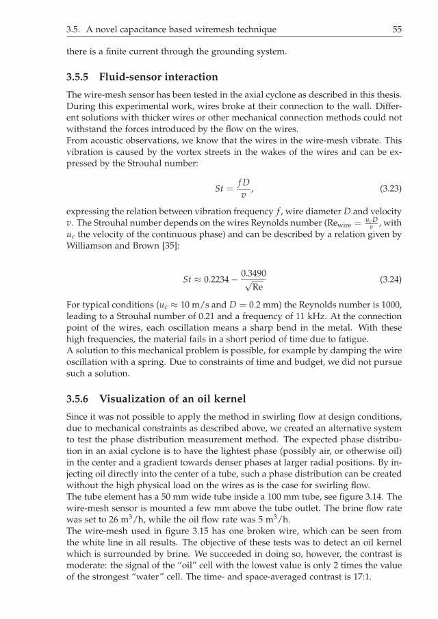
i

i

“Thesis1” — 2014/1/7 — 18:22 — page 55 — #75i

i

i

i

i

i


there is a finite current through the grounding system.

3.5.5 Fluid-sensor interaction

The wire-mesh sensor has been tested in the axial cyclone as described in this thesis.During this experimental work, wires broke at their connection to the wall. Differ-ent solutions with thicker wires or other mechanical connection methods could notwithstand the forces introduced by the flow on the wires.From acoustic observations, we know that the wires in the wire-mesh vibrate. Thisvibration is caused by the vortex streets in the wakes of the wires and can be ex-pressed by the Strouhal number:

St =f D

v, (3.23)

expressing the relation between vibration frequency f , wire diameter D and velocityv. The Strouhal number depends on the wires Reynolds number (Rewire = ucD

ν , withuc the velocity of the continuous phase) and can be described by a relation given byWilliamson and Brown [35]:

St ≈ 0.2234 − 0.3490√Re

(3.24)

For typical conditions (uc ≈ 10 m/s and D = 0.2 mm) the Reynolds number is 1000,leading to a Strouhal number of 0.21 and a frequency of 11 kHz. At the connectionpoint of the wires, each oscillation means a sharp bend in the metal. With thesehigh frequencies, the material fails in a short period of time due to fatigue.A solution to this mechanical problem is possible, for example by damping the wireoscillation with a spring. Due to constraints of time and budget, we did not pursuesuch a solution.

3.5.6 Visualization of an oil kernel

Since it was not possible to apply the method in swirling flow at design conditions,due to mechanical constraints as described above, we created an alternative systemto test the phase distribution measurement method. The expected phase distribu-tion in an axial cyclone is to have the lightest phase (possibly air, or otherwise oil)in the center and a gradient towards denser phases at larger radial positions. By in-jecting oil directly into the center of a tube, such a phase distribution can be createdwithout the high physical load on the wires as is the case for swirling flow.The tube element has a 50 mm wide tube inside a 100 mm tube, see figure 3.14. Thewire-mesh sensor is mounted a few mm above the tube outlet. The brine flow ratewas set to 26 m3/h, while the oil flow rate was 5 m3/h.The wire-mesh used in figure 3.15 has one broken wire, which can be seen fromthe white line in all results. The objective of these tests was to detect an oil kernelwhich is surrounded by brine. We succeeded in doing so, however, the contrast ismoderate: the signal of the “oil” cell with the lowest value is only 2 times the valueof the strongest “water” cell. The time- and space-averaged contrast is 17:1.

i

i

“Thesis1” — 2014/1/7 — 18:22 — page 56 — #76i

i

i

i

i

i


oil

brine

WMS sensor

Figure 3.14: Schematic of the setup to create a low-velocity oil kernel at the wire-mesh, figureis not to scale

3.5.7 Discussion and Conclusion

In this study, we combined existing wire-mesh components to form a system cap-able of measuring in liquids with a high conductivity. The measured variable isthe relative permittivity ǫr which proves to be a discriminating parameter for manygases and liquids. For the conducting phase ǫr is not measured - due to a groundedplane the measured value is 0 in these regions.Tests with a two phase oil/water system show the capability of distinguishing thetwo phases with a minimum contrast of at least 2:1 and an average contrast of 17:1.These values are obtained with an unmodified electronics box and software. Byoptimizing the timing of sampling of the receiving wires, this contrast should besignificantly improved.For measurements in liquid-liquid cyclones, wire fatigue is problematic. The flowintroduces high-frequency vibrations in the wires, which fail in a rather short timeat the connection point to the wall.

i

i

“Thesis1” — 2014/1/7 — 18:22 — page 57 — #77i

i

i

i

i

i


10 20 30

5

10

15

20

25

30

0

0.2

0.4

0.6

0.8

1

(a) t = 0.0 s

10 20 30

5

10

15

20

25

30

0

0.2

0.4

0.6

0.8

1

(b) t = 0.1 s

10 20 30

5

10

15

20

25

30

0

0.2

0.4

0.6

0.8

1

(c) t = 0.2 s

10 20 30

5

10

15

20

25

30

0

0.2

0.4

0.6

0.8

1

(d) t = 0.3 s

Figure 3.15: Four snapshots of the phase distribution measurement with the capacitancebased wire-mesh system.

i

i

“Thesis1” — 2014/1/7 — 18:22 — page 58 — #78i

i

i

i

i

i

58

i

i

“Thesis1” — 2014/1/7 — 18:22 — page 59 — #79i

i

i

i

i

i

CHAPTER 4

Strength of generated swirl

This chapter describes the liquid velocity profile for different swirl elements used inthis thesis. It aims at understanding the flow pattern generated by a specific swirlelement and deducing the acceleration in the radial direction experienced by thedroplets.

4.1 Theory

The acceleration of a dispersed liquid-liquid system can lead to the break-up ofdroplets. Since larger droplets can be separated with a weaker centrifugal pressurefield, it is preferable to design a cyclone such that droplets will not break belowa critical size or will not break at all. This section discusses models to predict thedroplet break-up behavior.

4.1.1 Force balances

Droplets can exist due to the interfacial tension force. Forces acting on the interface,such as shear and viscous forces, deform the droplets. If these forces exceed theinterfacial tension force by a critical extent, the droplet will break into two or moresmaller droplets.The critical value for droplet break-up is given by the Weber number and the Ca-pillary number:

Weber: We =shear force

interfacial tension force=

∣∣~t∣∣ Dd

σ, (4.1)

Capillary: Ca =viscous force

interfacial tension force=

µu

σ, (4.2)

with ~t the shear on the droplet, Dd the droplet diameter, σ the interfacial tensionbetween dispersed and continuous phase, µ the dynamic viscosity and u the char-acteristic velocity.

59

i

i

“Thesis1” — 2014/1/7 — 18:22 — page 60 — #80i

i

i

i

i

i

60 Chapter 4. Strength of generated swirl

For flows at high Reynolds numbers (Re > 1000) such as in industrial cyclones, theshear forces dominate over viscous forces.The actual force balance of the Weber number can be written in many differentways. Below, I will introduce some well known and convenient formats.

Acceleration induced breakup

Droplets experiencing a large enough shear force are prone to be torn in multiplepieces. This effect is known as shear induced droplet break-up, for which the inter-facial tension force (Fσ = σdπDd) tries to keep the droplet together, while the shearforces (tπD2

d, with t the tangential force per unit area) try to tear the droplet apart.The balance of these forces is given by the Weber number (We) which is introducedabove.According to experimental results discussed by Kolev [36] the critical Weber num-ber depends on the Reynolds number, but for Re > 2000 it is reasonable to approx-imate the critical Weber number as Wecritical = 5.The tangential force per unit surface t is estimated as the drag force divided by thesurface area of the droplet (assumed to be a sphere):

~t =~Fdrag

πD2d

=18

CDρc

∣∣∣∆~uslip

∣∣∣ ∆~uslip, (4.3)

with ∆~uslip the difference between the droplet velocity and the continuous phasevelocity surrounding. From the two equations above, the critical velocity is derived:

∆uslip >

√8Wecritσd

CDρcDd. (4.4)

The following example is based on typical conditions of the research in this thesis(with σd ≈ 30.10−3 N/m and ρc ≈ 1000 kg/m3). For the maximum local velocityoccurring in numerical simulations [13] (|umax| = 18 m/s), the maximum dropletReynolds number for a 10µm droplet is approximately 200, which leads to a CD ≈0.7 (see Appendix D). The critical size is then given by:

∣∣∣∆~uslip

∣∣∣2

Dd,crit = 1.7 · 10−3[

m3

s2

], (4.5)

which this provides a maximum stable droplet size of 5 µm with the assumptionthat the droplet is accelerated instantaneously to the terminal velocity. The estim-ated maximum droplet size is therefore judged to have a too small value, sincelarger droplets are found, as we will see in chapter 6.

Break-up by turbulent eddies

Hinze [37] proposed a model for the maximum droplet size in turbulent flow:

Dmax

(ρc

σ

)3/5ǫ2/5 = 0.725, (4.6)

where ρc is the density of the continuous phase and ǫ the turbulent dissipation rate.

i

i

“Thesis1” — 2014/1/7 — 18:22 — page 61 — #81i

i

i

i

i

i

4.1. Theory 61

The appropriate estimation of ǫ is essential for a correct prediction of the maximumdroplet size. The turbulent length scale can be estimated by:

ℓ =

(ν3

ǫ

)1/4

= ℓ0Re−3/4, (4.7)

where ν is the kinematic viscosity and ℓ0 the scale of the largest eddy (the tubediameter). Taking this into account, the turbulent kinetic energy can be expressedas:

ǫ =ν3Re3

ℓ40

. (4.8)

Figure 4.1 relates the maximum droplet size according to Hinze’s model (equation4.6) to the flow rate. At nominal conditions for the flow rig used in this investigationthe flow rate equals 56.5 m3/h, so that the maximum droplet size is predicted tobe 0.23 mm. As could be expected, a lower flow rate results in a larger maximumdroplet size.

0 10 20 30 40 50 60 70 80

10-4

10-3

10-2

1.9 mm

0.23 mm

flow rate (φ) [m3/h]

max

size

(Dm

ax)

[m]

Figure 4.1: Maximum droplet size as function of the flow rate, according to equation 4.6, fora 10cm tube with a flow rate of 56 m3/h with a continuous liquid density of 1064 kg/m3.

Break-up by strain

The strain rate γ is the magnitude of the velocity gradient tensor. The velocity dif-ference across the droplet is proportional to the strain rate. Within the actual staticswirl element and downstream tubing, the largest strain occurs close to the walls.Especially swirling flow is pushed towards the wall, leading to high velocity gradi-ents. Actual velocity measurements, as in figure 4.6 indicate a distance between the

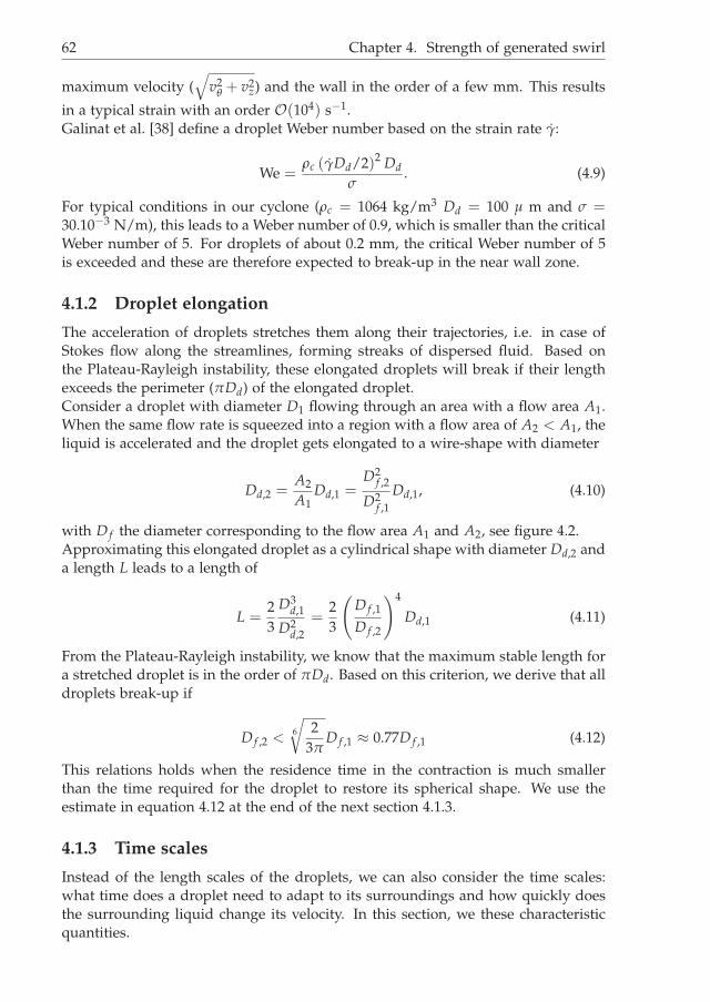
i

i

“Thesis1” — 2014/1/7 — 18:22 — page 62 — #82i

i

i

i

i

i


maximum velocity (√

v2θ + v2

z) and the wall in the order of a few mm. This results

in a typical strain with an order O(104) s−1.Galinat et al. [38] define a droplet Weber number based on the strain rate γ:

We =ρc (γDd/2)2 Dd

σ. (4.9)

For typical conditions in our cyclone (ρc = 1064 kg/m3 Dd = 100 µ m and σ =30.10−3 N/m), this leads to a Weber number of 0.9, which is smaller than the criticalWeber number of 5. For droplets of about 0.2 mm, the critical Weber number of 5is exceeded and these are therefore expected to break-up in the near wall zone.

4.1.2 Droplet elongation

The acceleration of droplets stretches them along their trajectories, i.e. in case ofStokes flow along the streamlines, forming streaks of dispersed fluid. Based onthe Plateau-Rayleigh instability, these elongated droplets will break if their lengthexceeds the perimeter (πDd) of the elongated droplet.Consider a droplet with diameter D1 flowing through an area with a flow area A1.When the same flow rate is squeezed into a region with a flow area of A2 < A1, theliquid is accelerated and the droplet gets elongated to a wire-shape with diameter

Dd,2 =A2

A1Dd,1 =

D2f ,2

D2f ,1

Dd,1, (4.10)

with D f the diameter corresponding to the flow area A1 and A2, see figure 4.2.Approximating this elongated droplet as a cylindrical shape with diameter Dd,2 anda length L leads to a length of

L =23

D3d,1

D2d,2

=23

(D f ,1

D f ,2

)4

Dd,1 (4.11)

From the Plateau-Rayleigh instability, we know that the maximum stable length fora stretched droplet is in the order of πDd. Based on this criterion, we derive that alldroplets break-up if

D f ,2 <6

√2

3πD f ,1 ≈ 0.77D f ,1 (4.12)

This relations holds when the residence time in the contraction is much smallerthan the time required for the droplet to restore its spherical shape. We use theestimate in equation 4.12 at the end of the next section 4.1.3.

4.1.3 Time scales

Instead of the length scales of the droplets, we can also consider the time scales:what time does a droplet need to adapt to its surroundings and how quickly doesthe surrounding liquid change its velocity. In this section, we these characteristicquantities.

i

i

“Thesis1” — 2014/1/7 — 18:22 — page 63 — #83i

i

i

i

i

i

4.1. Theory 63

Particle relaxation time

The droplets need to adapt to the velocity of the surrounding fluid - the fluid ac-celerates due to conservation of angular momentum and its incompressibility. Thedispersed phase therefore experiences a drag force which accelerates the droplets.For the design of the tapered section it is important that the acceleration of theliquid is such that the maximum slip velocity, i.e. the velocity difference betweencontinuous phase and dispersed phase is limited.The equation of motion of a dispersed droplet driven by the drag force of the sur-rounding continuous phase is given by [39]:

π

6

(ρd +

12

ρc

)D3

d

d~v

dt=

CD

2πD2

d

4ρc (~u −~v) |~u −~v| , (4.13)

with ~u the continuous phase velocity and~v the dispersed phase velocity. In equation4.13, we include the virtual mass effect, but we neglect other contributions to the

force on the droplets. In this equation the droplet Reynolds number Red = ρcDd |~u−~v|µc

can be substituted to get:

d~v

dt=

18µc(ρd + 1

2 ρc

)D2

d

CDRed

24(~u −~v) (4.14)

For low droplet Reynolds numbers, which are likely to occur for the small dropletshaving a moderate velocity difference with the surrounding liquid, we may assumeStokes flow: CDRed

24 ≈ 1. We introduce the characteristic time scale

τd =

(ρd + 1

2 ρc

)D2

d

18µc(4.15)

such that the original equation of motion can be approximated by

dv

dt=

1τp

(~u −~v) . (4.16)

A droplet will adjust to 1−ee of the terminal velocity within the particle relaxation

time τp.For conditions typical in this research (ρd = 872 kg/m3, µc ≈ 1.10−3 Pas), thecharacteristic time scale of the droplet ranges from O(10−5) s for a 10 µm dropletto O(10−3) s for a 250 µm droplet.

Timescale of the acceleration

Consider the fluid moving through a sudden contraction, where the diameter of thetube with circular cross section is reduced from D f 1 to D f 2 for a fluid path length ofL. Due to the incompressibility of the fluid and conservation of mass, the velocityin the latter surface is

v2 =D2

f 1

D2f 2

v1 (4.17)

i

i

“Thesis1” — 2014/1/7 — 18:22 — page 64 — #84i

i

i

i

i

i


The time scale for the contraction is estimated by dividing the path length L for thefluid by the mean velocity:

τf =L

12 (v1 + v2)

(4.18)

L

Df1 v

1 v2

Df2

α

Figure 4.2: Sketch for the estimation of the time scale in a gradual contraction.

For characteristic conditions in this research (v1 ≈ 2 m/s, D f 1/D f 2 ≈ 2 and L ≈ 0.1m), the time scale τf is in O(10−2) s. This is larger than the particle relaxation timescale τp.

Droplet restoration time

Droplets are deformed by forces acting on their surface. The interfacial tensiontends to keep the droplet in a spherical shape to reach a minimum energy.The restoration from a deformed state to a spherical shape can be treated as adamped harmonic oscillator, for which we will employ the following parameters:

• Dd: diameter of the undisturbed droplet

• m = π6 ρdD3

d: droplet mass

• x displacement parameter, given by the difference between the actual dropletperimeter and the undisturbed one (πDd).

The forces included in the equation of motion are:

• Spring force: caused by interfacial tension, Fs ∼ −σx;

• Viscous damping force: caused by viscous friction Fµ ∼ −µd x Dd2 .

Leading to the equation of motion:

mx = −σx − µdDd x. (4.19)

To derive an estimate for the maximum velocity of the droplet contraction, we con-sider the position at which x = 0 and the deformation velocity x is at its maximum.Then:

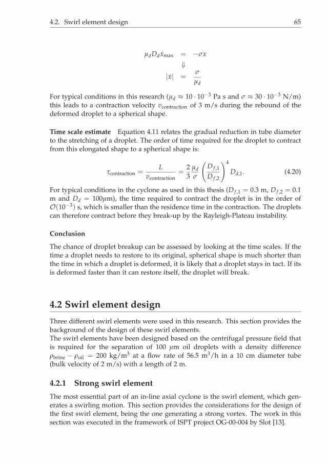
i

i

“Thesis1” — 2014/1/7 — 18:22 — page 65 — #85i

i

i

i

i

i

4.2. Swirl element design 65

µdDd xmax = −σx

⇓|x| =

σ

µd

For typical conditions in this research (µd ≈ 10 · 10−3 Pa s and σ ≈ 30 · 10−3 N/m)this leads to a contraction velocity vcontraction of 3 m/s during the rebound of thedeformed droplet to a spherical shape.

Time scale estimate Equation 4.11 relates the gradual reduction in tube diameterto the stretching of a droplet. The order of time required for the droplet to contractfrom this elongated shape to a spherical shape is:

τcontraction =L

vcontraction=

23

µd

σ

(D f ,1

D f ,2

)4

Dd,1. (4.20)

For typical conditions in the cyclone as used in this thesis (D f ,1 = 0.3 m, D f ,2 = 0.1m and Dd = 100µm), the time required to contract the droplet is in the order ofO(10−3) s, which is smaller than the residence time in the contraction. The dropletscan therefore contract before they break-up by the Rayleigh-Plateau instability.

Conclusion

The chance of droplet breakup can be assessed by looking at the time scales. If thetime a droplet needs to restore to its original, spherical shape is much shorter thanthe time in which a droplet is deformed, it is likely that a droplet stays in tact. If itsis deformed faster than it can restore itself, the droplet will break.

4.2 Swirl element design

Three different swirl elements were used in this research. This section provides thebackground of the design of these swirl elements.The swirl elements have been designed based on the centrifugal pressure field thatis required for the separation of 100 µm oil droplets with a density differenceρbrine − ρoil = 200 kg/m3 at a flow rate of 56.5 m3/h in a 10 cm diameter tube(bulk velocity of 2 m/s) with a length of 2 m.

4.2.1 Strong swirl element

The most essential part of an in-line axial cyclone is the swirl element, which gen-erates a swirling motion. This section provides the considerations for the design ofthe first swirl element, being the one generating a strong vortex. The work in thissection was executed in the framework of ISPT project OG-00-004 by Slot [13].

i

i

“Thesis1” — 2014/1/7 — 18:22 — page 66 — #86i

i

i

i

i

i


Azimuthal acceleration

The first design for an in-line swirl element was based on various assumptions. Thissection introduces the assumptions and concludes with the summary of the basicdesign parameters.

1. Separating force The rotating motion of the continuous phase exerts a pressureon a dispersed droplet which would maintain a droplet with no density differencein a circular motion with constant radius. A droplet with a larger density thanthat of the continuous phase lacks enough inward force to maintain the same radialdistance and spirals outward, a droplet with a smaller density than that of thecontinuous phase is pushed more inward than required for a circular motion withconstant radius and spirals therefore inward. The net force, pointing inward, is:

Finward(r) =πD3

d∆ρu2θ

6rd, (4.21)

with Dd the droplet diameter, ∆ρ the density difference (ρc − ρd), uθ the azimuthalvelocity of the continuous phase and rd the radial position of the droplet.This force accelerates the droplet in the radial direction, with a velocity differentfrom that of the surrounding liquid. This slip velocity induces a drag force which iscounteracting the accelerating force. For small droplet Reynolds numbers ( vsDd

ν ≪1), Stokes’ drag law can be applied:

Fstokes = 3πµDdvs, (4.22)

with µ the dynamic viscosity of the continuous phase and vs the settling velocity ofthe droplet. For a droplet moving at its settling velocity, we obtain the relation:

vr =∆ρD2

du2θ

18µrp, (4.23)

with vr the velocity of the droplet in the radial direction towards the center of thetube.

2. Velocity profile Dirkzwager [3] found that the velocity profile in an axial cyc-lone can be described reasonably accurate by the velocity distribution of the Burgersvortex:

uθ(r, z) = Uθ(z) for r > Rc, (4.24)

uθ(r, z) =Uθ(z)r

Rcfor r < Rc. (4.25)

Typical values for Rc of 0.25R have been reported [3].

3. Oil core The cyclone moves the lighter phase, oil, inward. The existence of anoil-continuous core in the center is therefore likely. When 10 % of the volume isoccupied by this core, this corresponds to a radius of 0.3Ri, which is larger than thecritical radius Rc in equations 4.24 and 4.25. The inward moving oil droplets aretherefore mostly in the outer region of the Burgers vortex for which vθ = constant.

i

i

“Thesis1” — 2014/1/7 — 18:22 — page 67 — #87i

i

i

i

i

i


4. Velocity coupling From the coupling between the axial and azimuthal velocitycomponents, the following relation for the droplet position as function of the axialdistance is derived:

vr =∂rd

∂t=

dz

dt

∂rd

∂z= vz

∂rd

∂z(4.26)

As a simple assumption, we apply the axial velocity to be equal to the bulk velocity:vz = ub. Over the length of the cyclone, the azimuthal velocity decays according to:

vθ(z) = vθ(0)e−zCd/D, (4.27)

with Cd an experimentally determined dimensionless parameter, determined to be0.04 [3] and D the tube diameter. Substitution of equations 4.26 and 4.27 in equation4.23 and subsequent integration, yields:

vz∂rd

∂z= −∆ρD2

d(vθ(0)e−zCd/D)2

18µrd, (4.28)

r2d(z) =

∆ρDD2dv2

θ(0)

18µCdub

(e−2zCd/D − 1

)+ r2

d(0). (4.29)

This equation can be interpreted as the equation of motion for any droplet withgiven properties in the specified swirling velocity field.

5. Droplet path For effective separation, the droplet has to move from its initialposition rd(0) to the oil core ( Dcore

D =√

α, α being the oil concentration) within theseparator length L:

rd(L) =12

D√

α (4.30)

The wall is the position from which the droplet has to travel the longest distance tothe core:

rd(0) =D

2. (4.31)

For the conditions in equations 4.30 and 4.31 and under the above mentioned as-sumptions, all droplets are separated. This results in a minimum requirement forthe azimuthal velocity of:

vθ(0)

ub= 3

D

Dd

√(1 − α)Cd

2(1 − e−2zCd/D

) 1

Red

with Red =∆ρubD

µ, (4.32)

or as a prediction for the cut-off size of:

Dd,crit =3

vθ(0)

√µCdubD(α − 1)

2∆ρ(e−2zCd/D − 1

) . (4.33)

i

i

“Thesis1” — 2014/1/7 — 18:22 — page 68 — #88i

i

i

i

i

i


Table 4.1: System properties used for the calculation of the required azimuthal acceleration

Quantity Unit Value

∆ρ [kg/m3] 190Dd [µm] 90L [m] 1.70ub [m/s] 2R [m] 0.05α [-] 0.1µ [Pa.s] 1e−3

Cd [-] 0.04

6. Neglected effects In the above mentioned analysis, we neglected many hy-drodynamic effects on the droplet. These effects include: (i) the dispersive effectof turbulent eddies, (ii) the lift force experienced due to a velocity gradient, (iii)droplet-droplet interactions, (iv) inner-droplet effects, such as flow in the dropletinduced by the drag force, (v) droplet-fluid coupling, the change of the continuousflow due to the presence of the droplets. The latter includes hindered settling, asdescribed by the Richardson & Zaki correlation [40], which is particularly relevantfor accounting repression of droplets towards the core. All these effects are expectedto have a counteractive effect on separation performance.

7. Conclusion From equation 4.32 and the values provided in table 4.1 the re-quired azimuthal velocity is calculated: 5.4 m/s. This corresponds to a certainamount of angular momentum of the continuous phase:

∣∣∣~L∣∣∣ =

∫ R

0(pθ × r) 2πrdr ≈ 2πρd

∫ R

Rc

vθ(0)r2dr =23

πρd(R3 − R3c )vθ(0), (4.34)

with ρd the droplet density and assuming that all angular momentum is in theregion r > Rc.According to equation 4.23, the maximum velocity for 100 µm droplets in the radialdirection is 0.15 m/s. The droplet Reynolds number for this velocity equals 15 - weviolate the condition for the Stokes’ drag law.

Inner body and vane angle

Static swirl elements consist of vanes mounted to the tube wall. At the tube center,these vanes need to be connected to a central body. Furthermore, the resultingazimuthal velocity is linked to the axial velocity at the swirl element and the vaneangle. For fixed vanes, there is a proportional relation between the axial velocityupstream and the azimuthal velocity downstream of the swirl element.In this section, we derive the required vane angle based on the required azimuthalvelocity calculated above, using the upstream axial velocity as boundary condition.

i

i

“Thesis1” — 2014/1/7 — 18:22 — page 69 — #89i

i

i

i

i

i


1. Axial velocity The static swirl element will transfer kinetic energy from theaxial direction towards the azimuthal direction to induce the swirling motion. Theelement consists of an internal body, centered at r = 0 and vanes connecting theinternal body to the wall of the tube. The diameter of the internal body is a designparameter: a thin body results in a low axial velocity and therewith steep vanes tocreate sufficient azimuthal acceleration; a thick internal body results in a high axialvelocity. The relation between the inner body radius Ri and the axial velocity isgoverned by conservation of mass:

uz,swirl = ubR2

R2 − R2i

. (4.35)

2. Angular momentum The swirl element should generate enough angular mo-mentum to generate the swirl velocity as prescribed by equation 4.32. The angularmomentum per unit of height h at a plane in the swirl element (SE) is:

LSE

h=

23

πρcuθ,swirl

(R3 − R3

i

), (4.36)

combined with equation 4.34 this yields the requirement for the azimuthal velocity:

uθ,swirl =R3 − R3

c

R3 − R3i

uθ(0)ρd

ρc. (4.37)

3. Vane angle The vanes deflect the flow from the axial direction to the azimuthaldirection. The relation between these is given by the vane angle, αdeflection:

αdeflection = arctan(

uθ,swirl

uz,swirl

)= arctan

(uθ(0)

ub

(R3 − R3

c

) (R2 − R2

i

)

R2(

R3 − R3i

) ρd

ρc

)(4.38)

A larger diameter Ri of the internal body has two effects: (i) the required vane angleis decreased and (ii) the velocity magnitude at the swirl element increases.The liquid acceleration at the swirl element results in the break-up of droplets.Vanes at a large angle and an acceleration to a high velocity result in droplet break-up. The total velocity increases substantially for Di > 0.8D, therefore, we chose thediameter of the internal body to be 80 mm. For this value, the relevant quantitiesare shown in the left column of table 4.2.

Table 4.2: Parameters for the vane design for 56.5 m3/h in a 10 cm diameter tube.

parameter no friction with friction compensation

αdeflection[] 62.6 74.3utot [m/s] 12.0 20.6uθ,swirl [m/s] 10.4 19.9uz,swirl [m/s] 5.6 5.6

i

i

“Thesis1” — 2014/1/7 — 18:22 — page 70 — #90i

i

i

i

i

i


Figure 4.3: Geometry of the vane in its local coordinate system. Inset: detail of the camberline and vane thickness. c is the chord length which is set to 100 mm. [13]

.

4. Frictional losses From previous work by Dirkzwager [3] it is known that 46 %of angular momentum was lost between the swirl element and the first measure-ment position at L/D = 10. To ensure enough separation according to the relationderived in section 4.2.1, the angular momentum at the downstream side of the swirlelement needs to be compensated, resulting in the column at the right of table 4.2.

Vane design

The fluid parameters at the downstream side of the swirl element were derived inthe preceding section. The vanes, which are mounted on the internal body, haveto convert potential energy (pressure) into angular momentum of the liquid. Toosudden changes in the fluid path can cause flow separation and therewith regionswith high shear. This shear exerts forces on droplets, causing break-up. Smallerdroplets have a lower chance of separation, this is the main reason why a gradualliquid acceleration along the vanes is important.The software package CASCADE [13] was used to find a vane shape which meetsthe criteria derived in this chapter. The vane shape is based on the NACA four-digitairfoil series [41]. With these tools, a vane was designed as shown in figure 4.3.The final design has vanes with αvane = 73.

Nose and afterbody design

The liquid should flow smoothly and without distortions from the upstream direc-tion towards the section with vanes. There are three criteria for this nose section:(i) r(z) is continuous, (ii) ∂r/∂z is continuous and (iii) both r(z) and ∂r/∂z shouldboth match at the vane section.The nose section is designed based on Hermite polynomials,. Slot [13] provides anextensive derivation of the procedure.

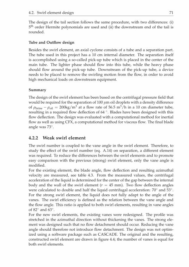
i

i

“Thesis1” — 2014/1/7 — 18:22 — page 71 — #91i

i

i

i

i

i


The design of the tail section follows the same procedure, with two differences: (i)5th order Hermite polynomials are used and (ii) the downstream end of the tail isrounded.

Tube and Outflow design

Besides the swirl element, an axial cyclone consists of a tube and a separation part.The tube used in this project has a 10 cm internal diameter. The separation itselfis accomplished using a so-called pick-up tube which is placed in the center of themain tube. The lighter phase should flow into this tube, while the heavy phaseshould flow around the pick-up tube. Downstream of the pick-up tube, a deviceneeds to be placed to remove the swirling motion from the flow, in order to avoidhigh mechanical loads on downstream equipment.

Summary

The design of the swirl element has been based on the centrifugal pressure field thatwould be required for the separation of 100 µm oil droplets with a density differenceof ρbrine − ρoil = 200kg/m3 at a flow rate of 56.5 m3/h in a 10 cm diameter tube,resulting in a required flow deflection of 64 . Blades have been designed with thisflow deflection. The design was evaluated with a computational method for inertialflow as well as using CFX, a computational method for viscous flow. The final bladeangle was 73.

4.2.2 Weak swirl element

The swirl number is coupled to the vane angle in the swirl element. Therefore, tostudy the effect of the swirl number (eq. A.14) on separation, a different elementwas required. To reduce the differences between the swirl elements and to promoteeasy comparison with the previous (strong) swirl element, only the vane angle ismodified.For the existing element, the blade angle, flow deflection and resulting azimuthalvelocity are measured, see table 4.3. From the measured values, the centrifugalacceleration of the liquid is determined for the center of the gap between the internalbody and the wall of the swirl element (r = 45 mm). Two flow deflection angleswere calculated to double and half the liquid centrifugal acceleration: 70 and 53.For the strong swirl element, the liquid does not fully adapt to the angle of thevanes. The swirl efficiency is defined as the relation between the vane angle andthe flow angle. This ratio is applied to both swirl elements, resulting in vane anglesof 82 and 63.For the new swirl elements, the existing vanes were redesigned. The profile wasstretched in the azimuthal direction without thickening the vanes. The strong ele-ment was designed such that no flow detachment should occur. Reducing the vaneangle should therefore not introduce flow detachment. The design was not optim-ized using a software package such as CASCADE. The original and the resulting,constructed swirl element are drawn in figure 4.4; the number of vanes is equal forboth swirl elements.

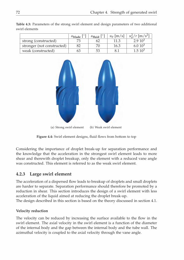
i

i

“Thesis1” — 2014/1/7 — 18:22 — page 72 — #92i

i

i

i

i

i


Table 4.3: Parameters of the strong swirl element and design parameters of two additionalswirl elements

αblade [] αfluid [] uθ [m/s] u2θ/r [m/s2]

strong (constructed) 73 62 11.3 2.9 103

stronger (not constructed) 82 70 16.3 6.0 103

weak (constructed) 63 53 8.1 1.5 103

(a) Strong swirl element (b) Weak swirl element

Figure 4.4: Swirl element designs, fluid flows from bottom to top

Considering the importance of droplet break-up for separation performance andthe knowledge that the acceleration in the strongest swirl element leads to moreshear and therewith droplet breakup, only the element with a reduced vane anglewas constructed. This element is referred to as the weak swirl element.

4.2.3 Large swirl element

The acceleration of a dispersed flow leads to breakup of droplets and small dropletsare harder to separate. Separation performance should therefore be promoted by areduction in shear. This section introduces the design of a swirl element with lessacceleration of the liquid aimed at reducing the droplet break-up.The design described in this section is based on the theory discussed in section 4.1.

Velocity reduction

The velocity can be reduced by increasing the surface available to the flow in theswirl element. The axial velocity in the swirl element is a function of the diameterof the internal body and the gap between the internal body and the tube wall. Theazimuthal velocity is coupled to the axial velocity through the vane angle.

i

i

“Thesis1” — 2014/1/7 — 18:22 — page 73 — #93i

i

i

i

i

i


Axial velocity The axial velocity in the swirl element depends on the size of theinternal body, i.e. the gap between the internal body and the surrounding wall.The axial velocity in the swirl element is given by the flow rate divided by the areaof the gap at the swirl element:

vz,swirl =Φ

Aflow, (4.39)

=Φ

π

((Rbody + dgap

)2− R2

body

) , (4.40)

=Φ

π(

2dgapRbody + d2gap

) , (4.41)

where φ is the flow rate in m3/s.

Azimuthal velocity The combination of a large diameter swirl element and the 10cm inner diameter tube as used for other tests in this work, requires a connectingtube element, a tapered section. Details of this section will be introduced in the nextsection, 4.2.4. For design purposes, we neglect friction and assume conservation ofangular momentum of the continuous phase over the length of the tapered section:

~L =~r ×~p. (4.42)

Since the position vector~r is orthogonal to the azimuthal velocity uθ , we obtain thefollowing relation for the velocity increase due to the tapering:

uθ,1

uθ,2=

|~r2||~r1|

, (4.43)

where index 1 is upstream of the tapered tube section and 2 downstream of thatsection.

Vane angle The vane angle depends on the relation between the axial and azi-muthal velocity according to:

tan(α) =uθ

uz(4.44)

The vane angle should not exceed 70 in order to avoid possible flow detachment.The strong and weak swirl element showed a difference in the resulting liquidvelocity angle and the vane angle. The same ratio is assumed to hold for the newswirl element. The vane angle is therefore increased with this slip factor (divide by0.85).

Number of vanes The number of vanes should be such that all liquid is acceler-ated in the azimuthal direction. The number of vanes should, however, not be thatlarge that the wall friction breaks more droplets. The number of vanes follows from

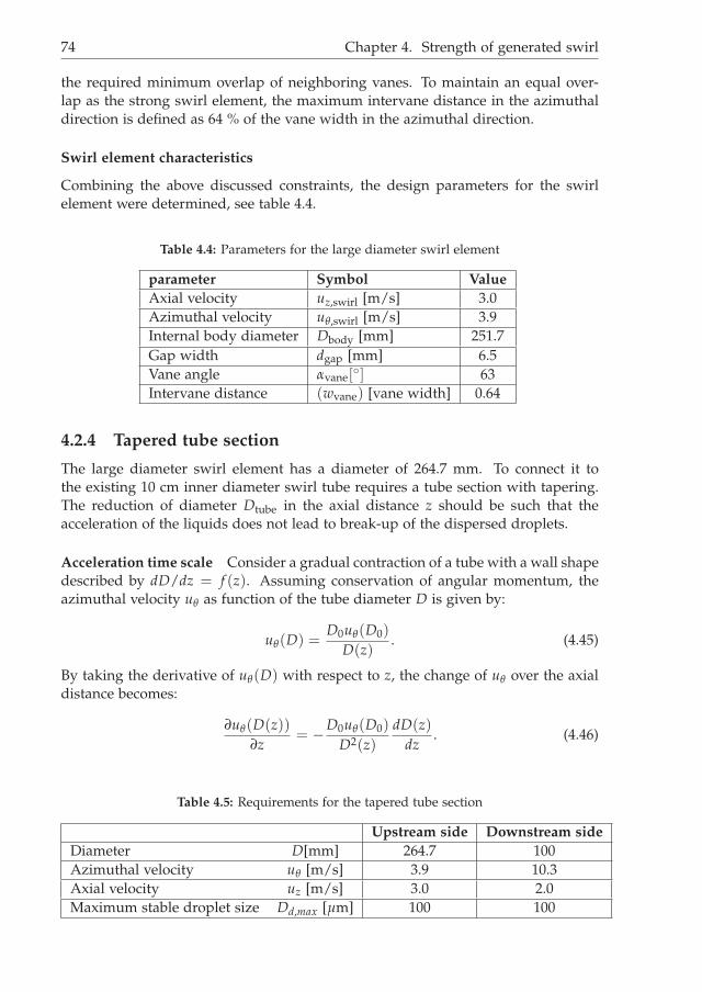
i

i

“Thesis1” — 2014/1/7 — 18:22 — page 74 — #94i

i

i

i

i

i


the required minimum overlap of neighboring vanes. To maintain an equal over-lap as the strong swirl element, the maximum intervane distance in the azimuthaldirection is defined as 64 % of the vane width in the azimuthal direction.

Swirl element characteristics

Combining the above discussed constraints, the design parameters for the swirlelement were determined, see table 4.4.

Table 4.4: Parameters for the large diameter swirl element

parameter Symbol Value

Axial velocity uz,swirl [m/s] 3.0Azimuthal velocity uθ,swirl [m/s] 3.9Internal body diameter Dbody [mm] 251.7Gap width dgap [mm] 6.5Vane angle αvane[] 63Intervane distance (wvane) [vane width] 0.64

4.2.4 Tapered tube section

The large diameter swirl element has a diameter of 264.7 mm. To connect it tothe existing 10 cm inner diameter swirl tube requires a tube section with tapering.The reduction of diameter Dtube in the axial distance z should be such that theacceleration of the liquids does not lead to break-up of the dispersed droplets.

Acceleration time scale Consider a gradual contraction of a tube with a wall shapedescribed by dD/dz = f (z). Assuming conservation of angular momentum, theazimuthal velocity uθ as function of the tube diameter D is given by:

uθ(D) =D0uθ(D0)

D(z). (4.45)

By taking the derivative of uθ(D) with respect to z, the change of uθ over the axialdistance becomes:

∂uθ(D(z))

∂z= −D0uθ(D0)

D2(z)

dD(z)

dz. (4.46)

Table 4.5: Requirements for the tapered tube section

Upstream side Downstream side

Diameter D[mm] 264.7 100Azimuthal velocity uθ [m/s] 3.9 10.3Axial velocity uz [m/s] 3.0 2.0Maximum stable droplet size Dd,max [µm] 100 100

i

i

“Thesis1” — 2014/1/7 — 18:22 — page 75 — #95i

i

i

i

i

i

4.3. Profile of the swirling flow 75

A measure for the time scale of the inward motion is the time the azimuthal velocityrequires to increase with (1 + e) times the original value. We estimate this timescale with a conservative estimate: a minimum tube diameter D of 10 cm, an axialvelocity uz of 2 m/s and the rest of the data provided in section 4.2.3 and table 4.2.4.This leads to:

∂uθ

∂t=

∂u

∂z· dz

dt,

= −D0uθ(D0)uz

D2(z)

dD(z)

dz,

≈ −adD

dzwith a ≈ 200

[ms2

].

Considering the azimuthal velocity at the upstream side of the taper, uθ = 4 m/s,the characteristic time-scale is the time required to increase uθ to 5.4 m/s. For theseconditions, the dependence on time-scale and dD/dz equals

τtaper = −7 · 10−3 [s]dD/dz

. (4.47)

The characteristic time scale for droplets to adapt to its surroundings (τd) is O(10−3)s, the time needed for the droplet to contract is τcontraction is also in O(10−3) s. Thetime scale of the displacement in the radial direction must be larger in order to avoidshear an elongation of the droplet and therewith break up. This implies dD/dz < 1.Based on the time estimate and the other design parameters, the constraints for thedesign of the tapering section are:

αupstream 0

αmax 40

αdownstream 0∂α∂z minimal and constant

rupstream 135 mmrdownstream 50 mm

Based on these parameters, Matlab has been used to numerically solve the shapeof the tapering section. Figure 4.5 shows the inner wall positions for the taperingsection.

4.3 Profile of the swirling flow

This section shows the effect of the swirl generating element on the resulting velo-city profile.The velocity profiles for the three different swirl elements are depicted in figure 4.6.There profiles are normalized with the axial bulk velocity as measured upstream ofthe swirl element.The azimuthal velocity in the region |r| < 10 mm is not affected that much bythe different swirl elements, the value ∂vθ/∂r is almost equal for all cases. The

i

i

“Thesis1” — 2014/1/7 — 18:22 — page 76 — #96i

i

i

i

i

i


-150 -100 -50 0 50 100 1500

50

100

150

200

250

tube radius (r) [mm]

axia

lpos

itio

n(z

)[m

m]

Figure 4.5: Numerical result for the calculation of the taper shape.

strength and size of the solid body rotating core are therefore almost swirl-elementindependent.The outside layer (|r| > 10 mm) is significantly influenced by the swirl element. Thestrong and weak element provide a relative flat profile with their respective max-ima at the edge of the solid-body rotating core that is proportional to the azimuthalvelocity at the swirl element. The large swirl element is different and generates sig-nificantly more swirl in the outside layers. The assumed slip between the vanes andthe liquid flow (see section 4.2.3) is much smaller than for the other two elements,the slip factor αflow/αvane is 0.94 instead of 0.85. The lower total velocity in theswirl element (5 m/s instead of 12 m/s) is a likely cause for the more efficient fluiddeflection - the residence time in the swirl element is namely inverse proportionalto the average axial velocity due to the equal vane size in the axial direction.The swirl elements are characterized by a swirl number, which we calculate accord-ing to equation A.14. Table 4.6 indicates the significant differences in swirl strengthbetween the strong and weak element. The swirl number for the large element isslightly larger than for the strong element, in contrast with the expectation basedon the azimuthal velocity in figure 4.6(a), where the azimuthal velocity for |r| > 20mm is larger than for the strong swirl element. However, the upstream velocityin the center region is larger for the large swirl element - this decreases the swirlnumber. As a correction, we introduce the following swirl number:

Ω′ =2π

∫ R0 |uzuθ | r′2dr′

πR3u2b

(4.48)

From the values of this swirl number Ω′ in table 4.6, the difference in swirl strengthbetween the different elements becomes clear.

i

i

“Thesis1” — 2014/1/7 — 18:22 — page 77 — #97i

i

i

i

i

i

4.3. Profile of the swirling flow 77

−50 −40 −30 −20 −10 0 10 20 30 40 50−8

−6

−4

−2

0

2

4

6

8


azim

uth

alvel

oci

ty(u

θ/u

b)

strong

weak

large

(a) azimuthal

−50 −40 −30 −20 −10 0 10 20 30 40 50−1.5

−1

−0.5

0

0.5

1

1.5

2

2.5


axia

lve

loci

ty(u

z/u

b)

strong

weak

large

(b) axial

Figure 4.6: Velocity profile for three different swirl elements, divided by the bulk velocity ub

upstream of the swirl element. Measurements obtained approximately 500 mm downstreamof the swirl element.Flow rate was 56 m3/h for the strong and weak swirl element and 30m3/h for the large swirl element.

4.3.1 Experimental conditions

The velocity profile was measured using Laser Doppler Anemometry (see section3.1). The laser was operated at an output power of approximately 3 W, measure-ment time interval per point was in the range of 5 to 10 s.LDA produces point measurements for the velocity. All measurement points are ona line parallel to the LDA probe through the center of the tube, resulting in meas-urements for the axial and azimuthal components of the velocity. Measurementpoints are typically 0.5 mm to 1.0 mm apart.

4.3.2 Strong swirl element

The velocity profile has been studied for single phase brine flow for all three swirlelements. Investigations of the strong swirl element are most elaborate. This sectiondiscusses the insights obtained with the strong swirl element.

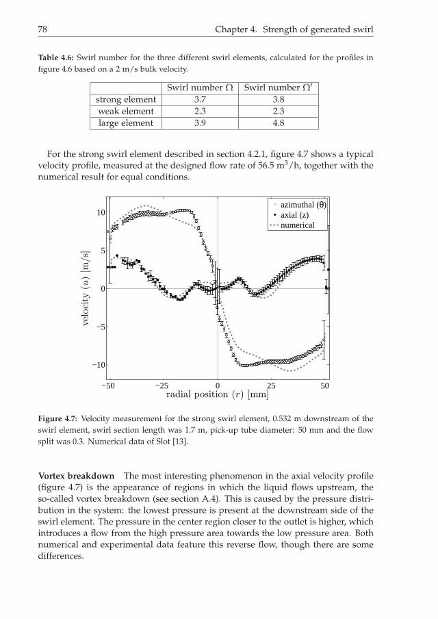
i

i

“Thesis1” — 2014/1/7 — 18:22 — page 78 — #98i

i

i

i

i

i


Table 4.6: Swirl number for the three different swirl elements, calculated for the profiles infigure 4.6 based on a 2 m/s bulk velocity.

Swirl number Ω Swirl number Ω′

strong element 3.7 3.8weak element 2.3 2.3large element 3.9 4.8

For the strong swirl element described in section 4.2.1, figure 4.7 shows a typicalvelocity profile, measured at the designed flow rate of 56.5 m3/h, together with thenumerical result for equal conditions.

−50 −25 0 25 50

−10

−5

0

5

10


velo

city

(u)

[m/s]

azimuthal (θ)

axial (z)

numerical

Figure 4.7: Velocity measurement for the strong swirl element, 0.532 m downstream of theswirl element, swirl section length was 1.7 m, pick-up tube diameter: 50 mm and the flowsplit was 0.3. Numerical data of Slot [13].

Vortex breakdown The most interesting phenomenon in the axial velocity profile(figure 4.7) is the appearance of regions in which the liquid flows upstream, theso-called vortex breakdown (see section A.4). This is caused by the pressure distri-bution in the system: the lowest pressure is present at the downstream side of theswirl element. The pressure in the center region closer to the outlet is higher, whichintroduces a flow from the high pressure area towards the low pressure area. Bothnumerical and experimental data feature this reverse flow, though there are somedifferences.

i

i

“Thesis1” — 2014/1/7 — 18:22 — page 79 — #99i

i

i

i

i

i

4.4. Properties of swirling flow 79

Swirl number The swirl number for this swirl element at this position has beencalculated according to equation A.14. The experimental data results in a swirlnumber of Ω = 3.7, which is about 10 % lower than the value predicted with thenumerical simulation [13]: Ω = 4.0. Apart from the significance of these numbers,the most likely cause is the presence of more friction in the real cyclone comparedto the perfect symmetric numerical case.

Solid body rotation zone The outer liquid layers (r > 35 mm) show a reason-able resemblance between the experimental and numerical data. The center regionseverely differs: the size of the solid-body rotation core is much larger for the nu-merical case than for the LDA measurements. The inertia in the real case apparentlyis dominant over viscosity in the radial direction. The physical cyclone has somedispersed oil in the center of rotation. This dispersed kernel can explain a step atthe kernel, but not the large difference in behavior for 0.1 <

rR < 0.6.

4.4 Properties of swirling flow

4.4.1 Vortex decay

Figure 4.8 illustrates the change in the velocity profile of the swirling brine forincreasing axial distance from the swirl element. This effect is driven by a decreasein angular momentum due to friction in the system. Apparently, the friction occursboth at the wall and in the center of the tube, since both regions loose angularmomentum in favor of the region around r ≈ 20 mm: The velocity increases forthat position from 10 m/s at z = 0.5 m to 12 m/s at z = 1.3 m.The LDA results are time-averaged velocity measurements. From these results it isclear that the time-averaged velocity at r = 0 is not always 0, as would be expectedfor an axial symmetric cyclone. Despite effort to optimize the alignment of thesystem and to avoid other sources that could trigger an asymmetry, we did notsucceed. Swirling axi-symmetric flow is not a stable situation.The discrepancies between the numerical data and the experimental results arenumerous. Except for the profile at z = 532 mm, the outer layer (r > 32 mm)is accurately predicted. The transition to a solid-body rotating kernel is for allmeasurements with z < 1300 mm calculated to be at a larger radial position thanactually observed in the experimental data. Consequently, the ∂uθ/∂r is smallerin the numerical simulation than for the velocity distribution determined usingLDA measurements. The applied treatment of the RANS approach with first orderclosure may not be capable of an accurate description of the swirling flow.The swirl number as introduced in equation A.14 is a measure for the strength ofthe swirling flow. Based on both the LDA and the numerical data, the swirl numberwas calculated for all axial locations presented in figure 4.8. Figure 4.9 presents therapid decrease in the swirl number for the cyclone in the experimental set-up. Thedecrease of swirl predicted by the numerical method is more gradual. An increasein friction due to the non-axi-symmetry could contribute to this difference.

i

i

“Thesis1” — 2014/1/7 — 18:22 — page 80 — #100i

i

i

i

i

i


−8 −4 0 −4 0 −4 0 −4 0 −4 0 −4 0 −4 00

10

20

30

40

50

radia

lpos

itio

n(r

)[m

m]

azimuthal velocity (uθ) [m/s]

430 mm

532 mm

725 mm

1100 mm

1200 mm

1305 mm

1430 mm

numerical

(a) azimuthal component

−8 −4 0 4 0 4 0 4 0 4 0 4 0 4 00

10

20

30

40

50

radia

lpos

itio

n(r

)[m

m]

axial velocity (uz) [m/s]

430 mm

532 mm

725 mm

1100 mm

1200 mm

1305 mm

1430 mm

numerical

(b) axial component

Figure 4.8: Measured and predicted velocities at different axial distances from the swirlelement. The graphs are shifted in axial direction for clarity. Numerical data of Slot [13].

4.4.2 Precessing Vortex Core

It is beyond the scope of this thesis to derive an analytical description for the pre-cessing vortex core. Alekseenko et al. [42] provide an extensive description, whileYazdabadi et al. [15] discuss the resulting measured velocities. From this exper-imental work, it is concluded that the center of the vortex is not always in thegeometrical center of the tube.To evaluate the possible existence of a precessing vortex core in the swirling flowused in the present study, we calculated the spectrum of the velocity data for variousconditions using ARMAsel [43]. Figure 4.10 shows six different spectra. Exceptfor the azimuthal velocity in the center with a short (5 s) time series, all profilesshow a peak around 43 Hz, indicating an autocorrelation in both the axial and theazimuthal velocity.If the core is precessing, this would show up as a cyclic sequence in the velocitydistribution, leading to a peak in the autocorrelation function. An alternative source

i

i

“Thesis1” — 2014/1/7 — 18:22 — page 81 — #101i

i

i

i

i

i


400 500 600 700 800 900 1000 1100 1200 1300 1400 15000

1

2

3

4

5

swir

lnum

ber

(Ω)

axial position (z) [mm]

LDA

numerical

Figure 4.9: Swirl number for different downstream distances of the swirl element obtainedfrom LDA and numerical velocity profiles

of this peak could be a vibration of the flow rig. The pump frequency for thesemeasurements was 43 Hz. Since that frequency is exactly the same as the frequencyin the autocorrelation spectra, it is not possible to attribute the peaks to a precessingvortex core. The 83 Hz peak is not present in all spectra. Other peaks are notobserved. From the single phase LDA data we can therefore not conclude on thatthere is a precessing vortex core.

0 20 40 60 80 100 120

10−3

10−2

10−1

frequency (f ) [Hz]

pow

ersp

ectr

alden

sity

(PS

D)

azimuthal near wall 30 s

azimuthal centre 30 s

axial near wall 30 s

axial centre 30 s

axial centre 5 s

azimuthal centre 5 s

Figure 4.10: Power spectral density of the LDA time series at different locations for the strongswirl element. Solid vertical lines are drawn for 43 Hz and 83 Hz.

4.4.3 Detail at the pick-up tube

At the downstream end of the tube with swirling flow, a pick-up tube is located.During multiphase flow conditions, the lighter phase ought to leave the separatortube through the pick-up tube, the heavy phase should leave through the annular

i

i

“Thesis1” — 2014/1/7 — 18:22 — page 82 — #102i

i

i

i

i

i


region surrounding the pick-up tube. The flow near the pick-up tube is therefore ofrelevance for the performance of the phase separator: additional shear can lead tobreak-up of droplets and disturb the possible formation of an oil-continuous kernel.The flow near the pick-up tube has been investigated in two ways: the velocityprofile in the annular ring has been measured with LDA and the velocity profilejust upstream of the pick-up tube has been measured with LDA, see figure 2.15.

Annular region

The size of the measurement volume is 0.2 mm in the radial direction, meaning thatthe measured velocity is an average over that distance. The position of the wall infigure 4.11 has been set to the point where both the axial and the azimuthal velocityare 0.Figure 4.11 presents velocity measurements for the axial and the azimuthal com-ponents of the velocity as function of the wall distance for the annular region sur-rounding the pick-up tube at 3 mm downstream of the leading edge of the pick-uptube. The azimuthal velocity does not slip at the wall, and a thin boundary layer isformed as is common for turbulent flows. An interesting phenomenon is observedfor the axial velocity component, which is pointing in the upstream direction in thelayer of the first 2 mm from the wall. This points at a pressure at the pick-up tubewall which is low at the upstream side of the pick-up tube and high at the down-stream side of the pick-up tube. This can be understood from the swirl strength asfunction of axial distance: the pressure gradient towards the wall is proportionalto the swirl strength. Since the swirl decays over length, the pressure at the outerwall of the pick-up tube is lowest at the pick-up tube tip and higher for positionsfurther downstream. This pressure difference can drive the observed upward flow.The numerical results as in figure 4.11 also features this near-wall reverse flow.

0 0.5 1 1.5 2 2.5 3−2

−1

0

1

2

3

4

5

radial wall distance (r) [mm]

vel

oci

ty(u

/ub)

uθ

uz

Numerical

Figure 4.11: Velocities near the pick-up tube, 3 mm downstream of the pick-up tube leadingedge. Wall position is derived from velocity measurements.

i

i

“Thesis1” — 2014/1/7 — 18:22 — page 83 — #103i

i

i

i

i

i


Just upstream of the pick-up tube

Just upstream of the pick-up tube, the fluid velocity must adjust in order to accom-modate the flow split - by changing the setting of the valves downstream of theoutflow section, the flow rate through both the LPO and HPO can be set. The cent-ral region with upstream flow (see figure 4.8(b)) that exists for the axial locationsup to 1430 mm has disappeared near the pick-up tube. The radial position of thepick-up tube is clear in the velocity profile as a dip in the axial velocity.

−8 −4 0 −8 −4 0 −8 −4 0 −8 −4 0 −8 −4 00

10

20

30

40

50

radia

lpos

itio

n(r

)[m

m]

azimuthal velocity (uθ) [m/s]

1600 mm

1625 mm

1650 mm

1675 mm

1700 mm

numerical

(a) azimuthal

0 1 2 0 1 2 0 1 2 0 1 2 0 1 20

10

20

30

40

50

radia

lpos

itio

n(r

)[m

m]

axial velocity (uz) [m/s]

1600 mm

1625 mm

1650 mm

1675 mm

1700 mm

numerical

(b) axial

Figure 4.12: Velocity profiles just upstream of the pick-up tube (at z = 1.7 m). Numericalresults are indicated.

i

i

“Thesis1” — 2014/1/7 — 18:22 — page 84 — #104i

i

i

i

i

i


4.5 Influence of operational parameters

4.5.1 Flow split effect

During operation of an axial cyclone, the distribution of the liquid streams over theHeavy Phase Outlet (HPO) and Light Phase Outlet (LPO) can be changed usingvalves downstream of the cyclone. The distribution of the streams over the twooutlets is called the Flow Split (FS) and is defined as:

FS =φLPO

φHPO + φLPO

, (4.49)

with φ the volumetric flow rate.The velocity profiles have been measured for different flow splits for all three swirlelements, see figures 4.13, 4.14 and 4.15.For the strong swirl element and weak swirl element, a higher flow split (moreliquid through the pick-up tube) leads to an increase of the azimuthal velocity inthe region |r| < 20 mm. This increase in angular momentum relates to an increasein the pressure drop, as can be seen in table 4.7.The total angular momentum was computed for the different flow splits accordingto an area-weighed method:

∣∣∣~L∣∣∣ ≈ 2

N(r=R)

∑i=1(r=0)

vθ(i)ρc∆zr(i)∆A(i)

∑Ni=1 ∆A(i)

(4.50)

with

∆A(i) = π

((r(i + 1) + r(i)

2

)2

−(

r(i) + r(i − 1)

2

)2)

(4.51)

and ∆z an infinitesimal height. Since both density ρc as ∆z are constant, we simplifyequation 4.50 to a relative version:

∣∣∣~L∣∣∣/(ρcdh) ≈ 2

N(r=R)

∑i=1(r=0)

vθ(i)r(i)∆A(i)

∑Ni=1 ∆A(i)

. (4.52)

Table 4.7 shows the results of this numerical operation and it demonstrates the sig-nificant reduction of the angular momentum with length and the relation betweenthe flow split and angular momentum.For the strong swirl element, a high pressure gradient following from the steep∂vθ∂r leads to a kernel consisting of dispersed material present in the cyclone. It

introduces additional noise for the measurements at r > 0 mm.The large swirl element (figure 4.15) is less sensitive to changes in the flow splitcompared to the strong and weak swirl element. Around |r| = 20 mm, the azi-muthal velocity increases for a larger flow split, while the overall profile shapechanges hardly.

i

i

“Thesis1” — 2014/1/7 — 18:22 — page 85 — #105i

i

i

i

i

i

4.5. Influence of operational parameters 85

−50 −40 −30 −20 −10 0 10 20 30 40 50−8

−6

−4

−2

0

2

4

6

8


azim

uth

alvel

oci

ty(u

θ/u

b)

FS = 0.2

FS = 0.3

FS = 0.4

(a) azimuthal

−50 −40 −30 −20 −10 0 10 20 30 40 50−1.5

−1

−0.5

0

0.5

1

1.5

2

2.5


axia

lvel

oci

ty(u

θ/u

b)

F = 0.2

F = 0.3

F = 0.4

(b) axial

Figure 4.13: Velocity profiles for three different flow splits, normalized with the liquid bulkvelocity. All profiles were obtained 532 mm downstream of the strong swirl element.

i

i

“Thesis1” — 2014/1/7 — 18:22 — page 86 — #106i

i

i

i

i

i


−50 −40 −30 −20 −10 0 10 20 30 40 50−8

−6

−4

−2

0

2

4

6

8


azim

uth

alvel

oci

ty(u

θ/u

b)

FS = 0.2

FS = 0.3

FS = 0.4

(a) azimuthal

−50 −40 −30 −20 −10 0 10 20 30 40 50

−1.5

−1

−0.5

0

0.5

1

1.5

2

2.5

3


axia

lvel

oci

ty(u

θ/u

b)

FS = 0.2

FS = 0.3

FS = 0.4

(b) axial

Figure 4.14: Velocity profile for three different flow splits for the weak swirl element, di-vided by the axial bulk velocity. All profiles were obtained at an axial distance of 532 mmdownstream of the swirl element for a flow rate of 42 m3/h.

i

i

“Thesis1” — 2014/1/7 — 18:22 — page 87 — #107i

i

i

i

i

i

4.5. Influence of operational parameters 87

Table 4.7: Angular momentum divided by density for the strong swirl element accordingto equation 4.52 for different downstream positions and different flow splits. The pressuredifference is measured between a point upstream of the swirl element and the LPO.

Relative angular momentum |~L|/(ρcdh)

[m2/s

]

z (mm) FS = 0.2 FS = 0.3 FS = 0.4532 0.43 0.42 0.43782 0.36 n.a. n.a.

1180 0.36 0.33 0.381430 0.25 0.34 0.34

∆p (bar) 1.79 1.83 1.90

Table 4.8: Swirl numbers for different flow rates and flow splits, calculated from velocitydata obtained with LDA.

[m3/h] FS = 0.2 FS = 0.3 FS = 0.4

strong element56 - 3.24 -42 3.12 3.32 3.39

weak element

56 - 2.30 -42 2.46 2.22 2.0530 - 2.05 -20 - 1.30 -

4.5.2 Effect of flow rate

The effect of flow rate on the velocity profile was compared for both the strongand the large swirl element. Figure 4.16 presents the profiles for the strong elementat 30, 42 and 56.5 m3/h, figure 4.18 contains the velocity distribution for the largeelement at 10, 20, 30 and 40 m3/h. All profiles are normalized with the bulk velocityfor appropriate comparability.The azimuthal velocity distribution shows limited dependence on the flow rate. Theazimuthal velocity increases more than proportional with flow rate, see the regionaround |r| = 10 mm in figure 4.16(a) and around |r| = 35 mm in figure 4.18(a). Thevariation of the velocity distribution increases more than proportional for increasingflow rate.The axial velocity for the strong swirl element (figure 4.16(b)) does not show notablechanges, except for an increase in variation of the velocity. The axial velocity of thelarge swirl element (figure 4.18(b)) appears to differ for changing flow rate. Theobserved changes can be explained by assuming a steady-state helical structurebetween the swirl element and the pick-up tube. By changing the flow rate, thewavelength of this structure changes, resulting in a different intersection of theLDA traverse with the vortex core. The 10 and 40 m3/h case appear to be flippedat r = 0 mm.

i

i

“Thesis1” — 2014/1/7 — 18:22 — page 88 — #108i

i

i

i

i

i


−50 −40 −30 −20 −10 0 10 20 30 40 50−8

−6

−4

−2

0

2

4

6

8


azim

uth

alvel

oci

ty(u

θ/u

b)

FS = 0.2

FS = 0.3

FS = 0.4

(a) azimuthal

−50 −40 −30 −20 −10 0 10 20 30 40 50

−1.5

−1

−0.5

0

0.5

1

1.5

2

2.5

3


axia

lvel

oci

ty(u

θ/u

b)

FS = 0.2

FS = 0.3

FS = 0.4

(b) axial

Figure 4.15: Velocity profile for three different flow splits for the large swirl element, di-vided by the axial bulk velocity. All profiles were obtained at an axial distance of 395 mmdownstream of the swirl element for a flow rate of 30 m3/h.

4.6 Conclusion

In this chapter, we introduced three different swirl elements to generate in-lineswirling flow and we investigated these elements using laser Doppler anemometry.The aim of these tests was to understand the fluid flow that results from a certainswirl element and to predict the phase separation performance resulting from theswirling flow.

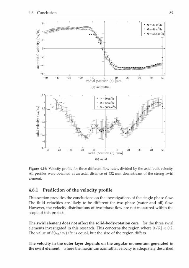
i

i

“Thesis1” — 2014/1/7 — 18:22 — page 89 — #109i

i

i

i

i

i

4.6. Conclusion 89

−50 −40 −30 −20 −10 0 10 20 30 40 50

−6

−4

−2

0

2

4

6


azim

uth

alvel

oci

ty(u

θ/u

b)

Φ = 30 m3/h

Φ = 42 m3/h

Φ = 56.5 m3/h

(a) azimuthal

−50 −40 −30 −20 −10 0 10 20 30 40 50−1.5

−1

−0.5

0

0.5

1

1.5

2

2.5


axia

lvel

oci

ty(u

θ/u

b)

Φ = 30 m3/h

Φ = 42 m3/h

Φ = 56.5 m3/h

(b) axial

Figure 4.16: Velocity profile for three different flow rates, divided by the axial bulk velocity.All profiles were obtained at an axial distance of 532 mm downstream of the strong swirlelement.

4.6.1 Prediction of the velocity profile

This section provides the conclusions on the investigations of the single phase flow.The fluid velocities are likely to be different for two phase (water and oil) flow.However, the velocity distributions of two-phase flow are not measured within thescope of this project.

The swirl element does not affect the solid-body-rotation core for the three swirlelements investigated in this research. This concerns the region where |r/R| < 0.2.The value of ∂(uθ/ub)/∂r is equal, but the size of the region differs.

The velocity in the outer layer depends on the angular momentum generated in

the swirl element where the maximum azimuthal velocity is adequately described

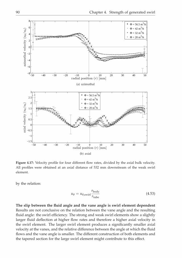
i

i

“Thesis1” — 2014/1/7 — 18:22 — page 90 — #110i

i

i

i

i

i


−50 −40 −30 −20 −10 0 10 20 30 40 50−8

−6

−4

−2

0

2

4

6

8


azim

uth

alvel

oci

ty(u

θ/u

b)

Φ = 56.5 m3/h

Φ = 42 m3/h

Φ = 32 m3/h

Φ = 20 m3/h

(a) azimuthal

−50 −40 −30 −20 −10 0 10 20 30 40 50

−1.5

−1

−0.5

0

0.5

1

1.5

2

2.5

3


axia

lvel

oci

ty(u

θ/u

b)

Φ = 56.5 m3/h

Φ = 42 m3/h

Φ = 32 m3/h

Φ = 20 m3/h

(b) axial

Figure 4.17: Velocity profile for four different flow rates, divided by the axial bulk velocity.All profiles were obtained at an axial distance of 532 mm downstream of the weak swirlelement.

by the relation:

uθ = uθ,swirlrbody

rtube(4.53)

The slip between the fluid angle and the vane angle is swirl element dependent

Results are not conclusive on the relation between the vane angle and the resultingfluid angle: the swirl efficiency. The strong and weak swirl elements show a slightlylarger fluid deflection at higher flow rates and therefore a higher axial velocity inthe swirl element. The larger swirl element produces a significantly smaller axialvelocity at the vanes, and the relative difference between the angle at which the fluidflows and the vane angle is smaller. The different construction of both elements andthe tapered section for the large swirl element might contribute to this effect.

i

i

“Thesis1” — 2014/1/7 — 18:22 — page 91 — #111i

i

i

i

i

i

4.6. Conclusion 91

−50 −40 −30 −20 −10 0 10 20 30 40 50−8

−6

−4

−2

0

2

4

6

8


azim

uth

alvel

oci

ty(u

θ/u

b)

Φ = 40 m3/h

Φ = 30 m3/h

Φ = 20 m3/h

Φ = 10 m3/h

(a) azimuthal

−50 −40 −30 −20 −10 0 10 20 30 40 50

−1.5

−1

−0.5

0

0.5

1

1.5

2

2.5

3


axia

lvel

oci

ty(u

θ/u

b)

Φ = 40 m3/h

Φ = 30 m3/h

Φ = 20 m3/h

Φ = 10 m3/h

(b) axial

Figure 4.18: Velocity profile for three different flow rates for the large swirl element, di-vided by the axial bulk velocity. All profiles were obtained at an axial distance of 395 mmdownstream of the swirl element.

4.6.2 Operational effects on phase separation

A higher flow rate leads to more centrifugal acceleration A higher flow rate leadsto a higher centrifugal acceleration according to:

Fc ∝ v2θ ∝ Φ2 (4.54)

However, it also introduces more turbulence, which can be seen from the largervariation in the velocity as is observed in this chapter. The effect of droplet break-up and turbulent dispersion is extensively discussed in chapter 5.

A higher flow split has a small favorable effect A higher flow split leads toregions in the cyclone with a larger azimuthal velocity. It can therefore lead to a

i

i

“Thesis1” — 2014/1/7 — 18:22 — page 92 — #112i

i

i

i

i

i


larger centrifugal acceleration of dispersed droplets, which on its turn might bebeneficial for the separation performance.

i

i

“Thesis1” — 2014/1/7 — 18:22 — page 93 — #113i

i

i

i

i

i

CHAPTER 5

Dispersed droplets in dilute swirling flow

The preceding chapter discussed the velocity profiles and derived quantities forsingle phase swirling flow. The aim of the swirling flow is to separate two phaseliquid-liquid streams. In this chapter, we use the experimental data obtained in thepreceding chapter to predict the droplet trajectories for dispersed oil droplets inswirling brine.The Reynolds number of the flow based on the bulk velocity and tube diameter inour cyclone is larger than 105 and it is therefore turbulent. The nature of turbulenceimplies fluctuations of the continuous phase fluid velocity in time, which affects thevelocity of the dispersed droplets. In this chapter, we derive a model for the dropletmotion based on experimental single phase flow data obtained for the three swirlelements.The ability to produce simple predictions of the effect of turbulence in swirling flowon dispersed droplets is of value for understanding the separation characteristicsand to aid design. The method suggested in this method is a hybrid approach,which should provide quicker results than Computational Fluid Dynamics alone.

5.1 Theory

The motion of the dense dispersed swirling flow can not be solved analytically, noris it possible with current technology to provide a numerical solution accuratelydescribing the behavior of each individual droplet. Therefore, we focus on a singledroplet moving in a single phase flow, which serves as a first reference for such adroplet in a dense multiphase flow.

Centrifugal acceleration

The liquid in the cyclone performs a swirling motion. The velocity of each fluidparcel can be decomposed in an axial (uz) and an azimuthal (uθ) component. Tomaintain the rotating motion in the radial plane, a centripetal force needs to beexerted on the liquid parcel at radial position r in the radial direction equal to:

93

i

i

“Thesis1” — 2014/1/7 — 18:22 — page 94 — #114i

i

i

i

i

i

94 Chapter 5. Dispersed droplets in dilute swirling flow

Fc =mu2

θ

r, (5.1)

with m the mass of the liquid element. This force points towards the axis of rotationof the swirling motion.Consequently, swirling flow has a pressure gradient in the radial direction. Fluidparcels with volume Vd experience the following centripetal force:

Fcentripetal =Vdρcu2

θ

r(5.2)

with ρc the density of the continuous phase.The force required to keep the droplet at a certain radial position r is given by thecentrifugal force:

Fcentrifugal =Vdρdu2

θ

r, (5.3)

with ρd the density of the dispersed phase.The net force driving the droplet within the rotating frame of reference is:

Fnet =Vd(ρd − ρc)u2

θ

r, (5.4)

this force points towards the center of the swirling motion if ρd < ρc and is thedriving force for centrifugal phase separation.

Drag force

An object which is moving through a viscous medium experiences a drag force. Ageneral expression for this force is [44]:

Fd =12

ρcu2relCD A, (5.5)

with urel the velocity of the object relative to the surrounding liquid, CD the dragcoefficient and A the projected area of the object perpendicular to the directionof motion. For the remainder of this chapter, we will assume the droplets in theliquid-liquid axial cyclone to be spherical.The drag coefficient depends on the droplet Reynolds number and therewith theviscosity of the surrounding fluid and the droplet velocity relative to the continuousfluid. For the remainder of this section we apply the empirical correlation for CD asproposed by Almedeij [45], which holds in the range Re < 106 and can be found inAppendix D.For low Reynolds numbers (Re< 1) the CD can be approximated by Stokes’ relationCD = 24

Re [39].

Turbulent dispersion

When the inertial forces in a fluid flow exceed the viscous forces, a flow becomesturbulent. A turbulent flow is characterized by momentum exchange between the

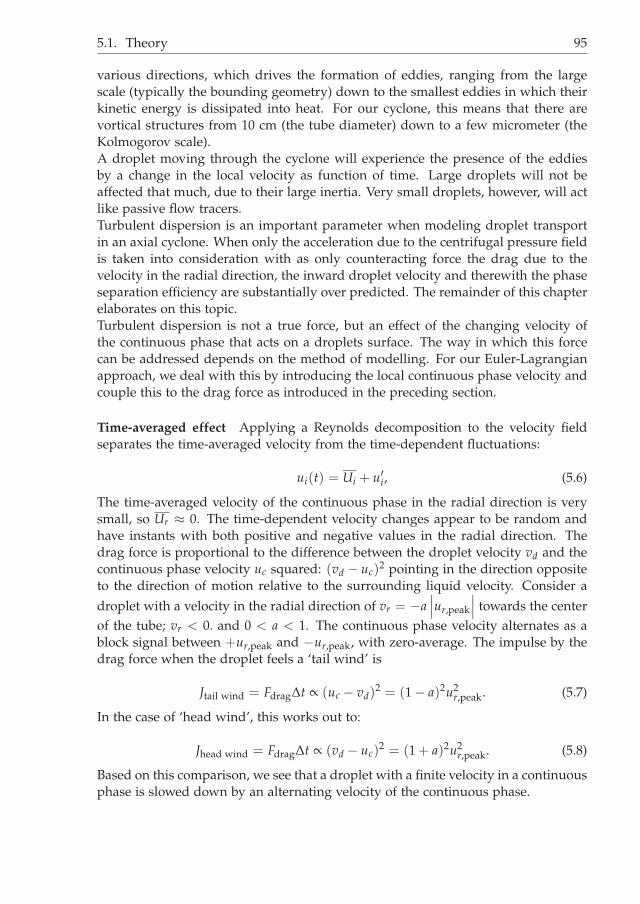
i

i

“Thesis1” — 2014/1/7 — 18:22 — page 95 — #115i

i

i

i

i

i

5.1. Theory 95

various directions, which drives the formation of eddies, ranging from the largescale (typically the bounding geometry) down to the smallest eddies in which theirkinetic energy is dissipated into heat. For our cyclone, this means that there arevortical structures from 10 cm (the tube diameter) down to a few micrometer (theKolmogorov scale).A droplet moving through the cyclone will experience the presence of the eddiesby a change in the local velocity as function of time. Large droplets will not beaffected that much, due to their large inertia. Very small droplets, however, will actlike passive flow tracers.Turbulent dispersion is an important parameter when modeling droplet transportin an axial cyclone. When only the acceleration due to the centrifugal pressure fieldis taken into consideration with as only counteracting force the drag due to thevelocity in the radial direction, the inward droplet velocity and therewith the phaseseparation efficiency are substantially over predicted. The remainder of this chapterelaborates on this topic.Turbulent dispersion is not a true force, but an effect of the changing velocity ofthe continuous phase that acts on a droplets surface. The way in which this forcecan be addressed depends on the method of modelling. For our Euler-Lagrangianapproach, we deal with this by introducing the local continuous phase velocity andcouple this to the drag force as introduced in the preceding section.

Time-averaged effect Applying a Reynolds decomposition to the velocity fieldseparates the time-averaged velocity from the time-dependent fluctuations:

ui(t) = Ui + u′i, (5.6)

The time-averaged velocity of the continuous phase in the radial direction is verysmall, so Ur ≈ 0. The time-dependent velocity changes appear to be random andhave instants with both positive and negative values in the radial direction. Thedrag force is proportional to the difference between the droplet velocity vd and thecontinuous phase velocity uc squared: (vd − uc)2 pointing in the direction oppositeto the direction of motion relative to the surrounding liquid velocity. Consider a

droplet with a velocity in the radial direction of vr = −a∣∣∣ur,peak

∣∣∣ towards the center

of the tube; vr < 0. and 0 < a < 1. The continuous phase velocity alternates as ablock signal between +ur,peak and −ur,peak, with zero-average. The impulse by thedrag force when the droplet feels a ‘tail wind’ is

Jtail wind = Fdrag∆t ∝ (uc − vd)2 = (1 − a)2u2

r,peak. (5.7)

In the case of ‘head wind’, this works out to:

Jhead wind = Fdrag∆t ∝ (vd − uc)2 = (1 + a)2u2

r,peak. (5.8)

Based on this comparison, we see that a droplet with a finite velocity in a continuousphase is slowed down by an alternating velocity of the continuous phase.

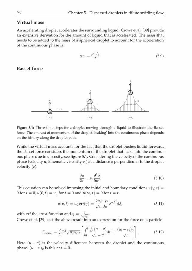
i

i

“Thesis1” — 2014/1/7 — 18:22 — page 96 — #116i

i

i

i

i

i


Virtual mass

An accelerating droplet accelerates the surrounding liquid. Crowe et al. [39] providean extensive derivation for the amount of liquid that is accelerated. The mass thatneeds to be added to the mass of a spherical droplet to account for the accelerationof the continuous phase is

∆m =ρcVd

2. (5.9)

Basset force

t = 0 t = t1

t = t2

v

v

v

u = 0

u

u

Figure 5.1: Three time steps for a droplet moving through a liquid to illustrate the Bassetforce. The amount of momentum of the droplet ‘leaking’ into the continuous phase dependson the history along the droplet path.

While the virtual mass accounts for the fact that the droplet pushes liquid forward,the Basset force considers the momentum of the droplet that leaks into the continu-ous phase due to viscosity, see figure 5.1. Considering the velocity of the continuousphase (velocity u, kinematic viscosity νc) at a distance y perpendicular to the dropletvelocity (v):

∂u

∂t= νc

∂2v

∂y2 . (5.10)

This equation can be solved imposing the initial and boundary conditions u(y, t) =0 for t = 0, u(0, t) = u0 for t = 0 and u(∞, t) = 0 for t = t:

u(y, t) = u0 erf(η) =2u0√

π

∫ η

0e−λ2

dλ, (5.11)

with erf the error function and η = y

2√

νct.

Crowe et al. [39] cast the above result into an expression for the force on a particle

FBasset =32

D2√πρcµc

[∫ t

0

ddt′ (u − v)√

t − t′dt′ +

(ui − vi)0√t

]. (5.12)

Here (u − v) is the velocity difference between the droplet and the continuousphase. (u − v)0 is this at t = 0.

i

i

“Thesis1” — 2014/1/7 — 18:22 — page 97 — #117i

i

i

i

i

i

5.1. Theory 97

0 0.2 0.4 0.6 0.8 1 1.2 1.4 1.6 1.8 210

−12

10−10

10−8

10−6

10−4

t/τ

F(N

)

DragBasset

Figure 5.2: Comparison of the magnitude of the Basset force (eq. 5.12) and the magnitudeof the drag force for an oil droplet of 10 µm accelerated in a centrifugal flow field with anazimuthal velocity of 10 m/s at a radial position of 40 mm

Order of magnitude Due to the complex nature of equation 5.12, we investigatethe influence of neglecting the Basset force for the accuracy of the droplet trajectory.To this end, we compare the drag force acting on a droplet which is accelerated inthe cyclone with the Basset force for the same droplet.The droplets acceleration is calculated using equation 5.17, for D = 10 µm, ud(t =0) = 0,ur = 0, ρd = 872 kg/m3, ρc = 1064 kg/m3, µc = 1.0 · 10−3 Pas and uθ=10m/s. The time step ∆t of the numerical integration was chosen such that a furtherdecrease in ∆t did not yield a noticeable improvement. ∆t was 0.5 · 10−3 s.Figure 5.2 clearly shows the significant difference between the drag force and theBasset force - the latter being about five orders of magnitude smaller. Therefore,it is reasonable to neglect the Basset force in further computations of the droplettrajectory.

Saffman lift force

The velocity in the cyclone is not uniform, therefore the droplets experience a velo-city gradient. This gradient develops a shear difference over the droplet, that createsa rotating motion. Based on the theory of Saffman [46] many authors elaborated onthe direction and magnitude of this so-called Saffman lift force.Crowe et al. [39] provide a convenient relationship for the magnitude of the force,being:

Fsaff = 1.61µcD |ui − vi|√

ReG, (5.13)

where the shear Reynolds number ReG is defined as:

ReG =D2

νc

du

dy. (5.14)

We compare the magnitude of the Saffman lift force with the magnitude of the dragforce for an oil droplet of 10 µm accelerated in a centrifugal flow field with an

i

i

“Thesis1” — 2014/1/7 — 18:22 — page 98 — #118i

i

i

i

i

i


0 0.2 0.4 0.6 0.8 1 1.2 1.4 1.6 1.8 210

−10

10−9

10−8

10−7

10−6

10−5

10−4

t/τ

F(N

)

DragSaffman Lift

Figure 5.3: Comparison of the magnitude of the Saffman lift force and the magnitude of thedrag force for an oil droplet of 10 µm accelerated in a centrifugal flow field with an azimuthalvelocity of 10 m/s at a radial position of 40 mm

azimuthal velocity of 10 m/s at a radial position of 40 mm in figure 5.3. To thisend, we use the same parameters as we used for the comparison in the precedingsection for the Basset force. For the velocity gradient ∂u

∂y , the maximum gradient

present in the cyclone was selected: duθdr at r = 0: duθ

dr = 3.25 · 103 s−1. For this case,the magnitude of the Saffman lift is about two orders of magnitude smaller thanthe drag force - therefore this effect will be neglected too.

5.2 Droplet model

In this section, we cast the physics into an equation of motion that can be solvednumerically. This is done using the theory derived in section 5.1.

5.2.1 Equation of motion

From section 5.1 we know that the following forces are relevant for the dropletsin our cyclone: the net centrifugal pressure, drag, turbulent dispersion and virtualmass.This leads to the equation of motion for an oil droplet accelerated in the watercontinuous cyclone:

π

6D3

d

(12

ρc + ρd

)dvr

dt︸︷︷︸Droplet acceleration,

including virtual mass

=π

6D3 (ρd − ρc) u2

θ

r︸︷︷︸Centrifugal buoyancy force

+π

8D2

dCD (Red) ρc (vr − ur)2

︸︷︷︸Drag force

. (5.15)

Recall that the liquid velocity is indicated with u, the droplet velocity with v. Theindex d denotes the droplet and c the continuous phase. In equation 5.15 the droplet

i

i

“Thesis1” — 2014/1/7 — 18:22 — page 99 — #119i

i

i

i

i

i

5.2. Droplet model 99

Reynolds number (acting in the radial direction, relative to the surrounding fluid)is:

Red =ρcD |u − v|

µc. (5.16)

Turbulent dispersion is included in the drag through the continuous phase velocityuc. We only take the turbulent dispersion in the radial direction into account; it isassumed that there is no slip between the droplet and the continuous phase in theaxial and azimuthal direction.For convenience, we rewrite the equation of motion in the radial direction to:

dv

dt=

1τd

CD(Red)Red

24(u − v) +

ρd − ρc12 ρc + ρd

u2θ

r(5.17)

with the droplet relaxation time:

τp =

(12 ρc + ρd

)D2

d

18µc. (5.18)

5.2.2 Experimental input to the model

The Laser Doppler Anemometry (LDA) measurements provide the velocity as func-tion of time for the axial and azimuthal velocity. The radial velocity is not measured.The velocity in the radial direction, and especially the time-dependent velocity fluc-tuations, determine to a great extent the drag experienced by the droplet movingin the radial direction. The time-averaged velocity in the azimuthal direction de-termines the centrifugal acceleration of the droplet towards the center and the axialvelocity is necessary to predict the residence time in the cyclone.Since we lack the measured velocity data for the radial direction, an assumptionis made for the radial velocity. Although the turbulence inside a swirling flow athigh Reynolds number cannot be assumed to be isotropic we nevertheless assumethat the magnitude and time scale of the radial velocity fluctuations is of the sameorder of magnitude as for the measured axial velocity component. The velocityof the azimuthal velocity is larger, where that component is confined by the tubewall. Therefore, the frequency and magnitude of the axial velocity will be morecomparable with the radial velocity statistics.This leads to the following relation for the velocity used in the model for the droplettrajectory, all experimentally obtained datasets, with the Reynolds decompositionapplied (u(t) = U + u′(t)):

Axial: uz(r, φ, z, t) = Uz(r)

Azimuthal: uθ(r, φ, z, t) = Uθ(r)Radial: ur(r, φ, z, t) = 0 + u′

z(r, t)The time-averages of the velocities Uz(r) and Uθ(r) are huge compared to the time-dependent velocity fluctuations (results described in section 4.3.2, example datasetin figure 5.6). The particle relaxation time τd is small compared to the residencetime of the droplet in the cyclone, therefore we can assume the droplet to have the

i

i

“Thesis1” — 2014/1/7 — 18:22 — page 100 — #120i

i

i

i

i

i


100

101

102

103

104

10−6

10−5

10−4

10−3

f (Hz)

A

Original signal

Resampled signal

Figure 5.4: Amplitude of the power spectrum of an original dataset and that of the recon-structed data

same velocity as the continuous phase in the z- and θ-direction. We calculate themovement of the droplet in the r-direction.

Frequency in LDA signal

Velocity measurements performed with Laser Doppler Anemometry (LDA) meas-ure the velocity of tracers dispersed in the flow. The frequency of the particlesarriving in the measurement volume is irregular, and therewith the LDA velocitytime series. Due to this irregularity, the signal contains frequency information ex-ceeding the sampling frequency (see Durst et al. [18]). According to Broersen [43],the frequency spectrum cannot be calculated using common methods like fast Four-ier transforms. Instead, we use the software package ARMAsel [43].ARMAsel computes the power spectrum of the original signal, which is used toconstruct a new velocity profile as function of time, according to:

v(ti) =fmax

∑fi=0

T

∑ti=0

PSD2 cos ( fi · (ti − t0)) (5.19)

The data is resampled at a frequency higher than the highest frequency obtained inthe original signal with ARMAsel. The time series is multiplied with a constant torender the variance of the signal equal to the variance of the original signal, whilethe mean value is kept at 0. The spectrum of the resulting time series is comparedwith the original spectrum. Figure 5.4 shows good agreement of the two spectra.The mean difference of the velocities of the droplets with the mean fluid velocity(v − u) has been calculated for a range of droplet sizes for a constant centrifugal ac-celeration according to equation 5.17. Figure 5.5 shows the difference in the velocityfor droplets between 15 and 70 µm.

i

i

“Thesis1” — 2014/1/7 — 18:22 — page 101 — #121i

i

i

i

i

i


100

101

102

10−1

100

101

102

D(µm)

v(m

/s)

Original dataset

Reconstructed dataset

Figure 5.5: Comparison of the averaged droplet velocity and the mean continuous phasevelocity for a constant centrifugal acceleration as function of droplet size for the originalLDA dataset and for the reconstructed data.

5.2.3 Numerical implementation

This section describes the strategy and the equations used for numerically solvingequation 5.17. Figure 5.6 depicts the scheme of the method to calculate the dropletposition and velocity.

Loop structure The particle trajectory is calculated for a range of droplet sizes Dd.Each time step , ∆t′, is chosen based on the interval between the chosen samples forthe radial velocity. The resulting time series is therefore irregular.

Input parameters The continuous phase is represented using the time-averagevelocity data for the azimuthal and axial direction and by a time series for the ra-dial velocity. This time series is estimated by using the velocity fluctuations in theaxial direction with zero average, as discussed in section 5.2.2, with 5 mm spacingbetween measurement points.

For each time step, the following data is stored for the droplet:

t′iv(t′i)r(t′i)

The properties of the continuous phase are obtained from the available datasets forthe same time instance:

uθ = Uθ(r)uz = Uz(r)

ur = ur(r, t′i)r(t′i)

i

i

“Thesis1” — 2014/1/7 — 18:22 — page 102 — #122i

i

i

i

i

i


v = 0

r = r0

Droplet initial conditions

Uz(r)

Uθ(r)

u′

r(r, t) with u

′

r= 0 in bins of ∆r = 5mm

Continuous phase input

v(t′

i)

r(t′i)

droplet position and velocity

and the continuous phase velocity

for each time step:

u = u(t′)

∆t′ = t

′

i+1− t

′

i

Rep =ρcD |u − v||

µc

v(t′i+1) = u +

ρd − ρc1

2ρc + ρd

τpv2

θ

r

+

(v(ti) − u −

ρd − ρc1

2ρc + ρd

τpv2

θ

r

)e−∆t′/τp

r(t′i+1) =

v(ti+1) + v(ti)

2∆t

′

Rep < 1

Rep > 1

0 5 10 15 20

−2

−1

0

1

2

t (ms)u

r(m

/s)

• no algebraic solution to the equation of motion

• division into n bins for approximate solution

v(t′′

i)

r(t′′i)

Rep =

ρcD|u−v′′(ti)||

µc

CD = CD(Rep)

v(t′′i+1) = u +ρd − ρc12ρc + ρd

24τp

CDRep

v2θ

r

+

(v(t′′i ) − u −

ρd − ρc12ρc + ρd

24τp

CDRep

v2θ

r

)e−CDRep∆t′′/(24τp)

r(t′′i+1) =v(t′′i+1) + v(t′′i )

2∆t

′′

Figure 5.6: Scheme of the numerical implementation to solve the droplet equation of motionin the axial cyclone

i

i

“Thesis1” — 2014/1/7 — 18:22 — page 103 — #123i

i

i

i

i

i


Equation of motion Based on the data available for each point, the net force on thedroplet is estimated for each time step. Using Newton’s second law, the droplet’strajectory is determined. The strategy for this estimation depends on the dropletReynolds number Red (equation 5.16). If Red < 1 an analytical solution (Stokesflow) exists for the equation of motion (equation 5.17), since then CDRep/24 ≈ 1.The equation of motion then simplifies to:

∂vr

∂t=

1τd

(ur − vr) +ρd − ρc

12 ρc + ρd

u2θ

r(5.20)

which is analytically solved for vr(0) = vr,0 to yield:

vr(t′i+1) = ur +ρd − ρc

12 ρc + ρd

τdu2

θ

r+

(vr(t′i) − ur −


τdv2

θ

r

)e−(t′i+1−t′i)/τd . (5.21)

When Red > 1 the equation of motion cannot be solved analytically due to thedependence of CD on the Reynolds number. It is not possible to assume CD to beconstant during an interval ∆t′, since we would then overestimate the drag exertedby the continuous phase on the droplet. To resolve this, the bin is split into aninteger number of n subbins that just fits the criterion ∆t′′ < τp. Within theseintervals, CD is kept constant. For each subbin, the approximate velocity is givenby:

vr(t′′i+1) =

(vr(t′′i ) − ur −


24τd

CDRedτd

v2θ

r

)e−CDRed(t′′i+1−t′′i )/(24τd)

+ ur +ρd − ρc

12 ρc + ρd

24τp

CDRedτp

u2θ

r, (5.22)

where we estimate for each time step:

CD(Rep) = CD(Rep(v(t′′i ))).

Axial displacement The solution for the position in the axial direction is straight-forwardly calculated by ∆z = Uz∆t′.

5.2.4 Droplet break-up

For each droplet being released in the system as described in this chapter, the pathand velocity can be calculated. We know from the theory discussed in section 4.1that droplets break-up when the shear forces on the interface exceed the force thatthe interfacial tension can withstand. This is expressed by the Weber number:

We =ρcD (v − u)2

σ, (5.23)

The critical Weber number at which the droplet breaks, depends on the droplet

Reynolds number Red = |v−u|Dν , according to a model proposed by Brauer [47]:

i

i

“Thesis1” — 2014/1/7 — 18:22 — page 104 — #124i

i

i

i

i

i


0 500 1000 1500 2000 25005

10

15

20

25

Red

We

Figure 5.7: Weber number as function of the droplet Reynolds number based on the relationin equation 5.24.

.

Wecrit =

24 for Red < 200

55(

24Red

+ 20.1807Re0.615

d

− 16Re2/3

d

)for 200 < Red < 2000

5.32 for Red > 2000

(5.24)

The critical Weber number is kept constant for Reynolds numbers smaller than 200at the value at Re = 200, being 24. For Re > 2000, the critical Weber number is keptconstant at 5.32. A graphical representation of this relation is in figure 5.7.For each time step t′ in figure 5.6, the velocity relative to the fluid (|u − v|) is com-pared with the critical velocity:

vcrit =

√Wecritσ

Dρc(5.25)

In case the slip velocity exceeds the critical velocity at any time step, the dropletis assumed to be broken apart. In this model, we count the number of brokendroplets, no tracking of the secondary droplets is done, since we cannot predict thesize of the droplet fragments.The LDA data used in the model has a random nature, both with respect to thesampling rate and turbulent velocity statistics. We therefore run the model re-peatedly with a different initial condition for the time-dependent fluid velocity.This provides us with the probability that a droplet of given size breaks up in thecyclone.

5.3 Dilute droplets simulation results

The basis of the model derived in this chapter cannot be used to describe the densemultiphase flow as is encountered in a liquid-liquid axial cyclone, simply because

i

i

“Thesis1” — 2014/1/7 — 18:22 — page 105 — #125i

i

i

i

i

i

5.3. Dilute droplets simulation results 105

Table 5.1: Available LDA datasets for the numerical method introduced in this chapter.

Flowrate [m3/h]Swirl Element 10 20 30 42 56Strong swirl x x xWeak swirl x x x x

Large swirl x x x x

0 0.2 0.4 0.6 0.8 1 1.2 1.4 1.60.01

0.015

0.02

0.025

0.03

0.035

0.04

0.045

0.05

axial position (z) [m]

radia

lposi

tion

(r)

[m]

D = 0.010 mm

D = 0.050 mm

D = 0.10 mm

D = 0.5 mm

Figure 5.8: Examples of simulated droplet paths for four different droplet sizes for the strongswirl element at 56 m3/h flow.

we approach the device as a dilute system in which the turbulence levels are asmeasured for the water-only case are true and we neglect any droplet-droplet inter-actions. However, the model is used to obtain insights why some droplets can andothers cannot be separated with our cyclone. The available LDA datasets are listedin table 5.1.From these available datasets, we make two comparisons: (i) an equal swirl ele-ment at different flow rates and (ii) three different swirl elements at an equal flowrate. For (i) we use the weak swirl element and for (ii) we use the flow rate ofapproximately 42 m3/h.An example of the raw output generated by the model introduced in this chapteris presented in figure 5.8. The trajectory for four different droplet sizes is plotted inits axial and radial coordinates based on the measured velocity data for the strongswirl element at 56 m3/h. Due to the random selection of the starting point in themodel, the result is different for each simulation batch.

i

i

“Thesis1” — 2014/1/7 — 18:22 — page 106 — #126i

i

i

i

i

i


5.3.1 Smallest separated droplets

Droplets with a small size (much smaller than the critical size dcrit) have a very smallτp and will follow each fluctuation in the continuous phase velocity. A very largedroplet (much larger than the critical size dcrit) will only follow the time averagevelocity. It is likely that droplets larger than dcrit will be separated in our cyclone,and droplets smaller than dcrit will not.The model as introduced in this chapter was used to evaluate the time required for arange of droplet sizes to reach the center of the tube (where r/R < 0.2), normalizedby the average residence of the liquid in the cyclone T (streamwise length dividedby the bulk velocity). If the time needed by a certain droplet to reach the center ofthe tube exceeds the residence time, we can be sure that it will not coalesce into apossible oil-continuous core.Figure 5.9(a) compares for four different flow rates in the weak swirl element thetime required to reach the center as function of the droplet size. For the threehighest flow rates, the separation time exceeds the residence time for droplets smal-ler than 50 µm. For the 20 m3/h case, the residence time is not exceeded. For allsimulations, it holds that the swirl decay with axial distance has not been considered- the LDA datasets were too limited to do so. The data used for these simulationswere obtained about 30 cm downstream of the swirl element and will therefore overpredict the separation performance. Droplets that need the order of the residencetime to get separated will therefore most likely not separate in reality. When we usea non-dimensional time t/T (time to center over residence time) of 0.5 as criterionfor separation, the smallest separated size is listed in table 5.2.

Table 5.2: Smallest droplet size that can be separated, based on the criterion that the t/T <

0.5.Flow rate Φ (m3 /h) Droplet size D ( µm)

56 9042 10030 11020 220

Figure 5.9(b) compares for the strong, weak and large swirl element the time re-quired for droplets to reach the center, where the droplets are assumed to stayintact. We see significant differences for the three swirl elements: the stronger swirlgenerated by the large element is capable to separate smaller droplets - already for60 µm, the time to get to the center is less than half of the residence time. The strongand weak swirl element perform nearly equal, the threshold of half the residencetime is passed for droplets smaller than 130 µm.

5.3.2 Droplet break-up

As we have seen in section 5.3.1, it is favorable to increase the flow rate as well asthe swirl strength to promote separation of droplets with a small diameter. Thedownside of this increase in flow rate or swirl strength is, however, that for a con-stant droplet diameter the velocity difference between the droplet and that of the

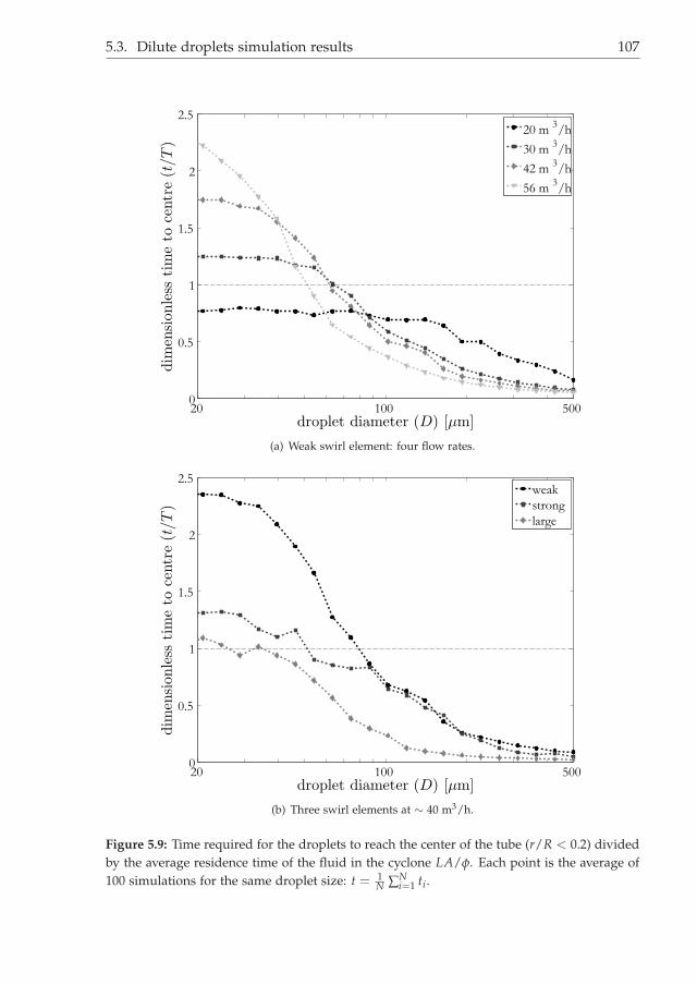
i

i

“Thesis1” — 2014/1/7 — 18:22 — page 107 — #127i

i

i

i

i

i


20 100 5000

0.5

1

1.5

2

2.5

droplet diameter (D) [µm]

dim

ensi

onle

ssti

me

toce

ntr

e(t

/T

)

20 m3/h

30 m3/h

42 m3/h

56 m3/h

(a) Weak swirl element: four flow rates.

20 100 5000

0.5

1

1.5

2

2.5


dim

ensi

onle

ssti

me

toce

ntr

e(t

/T)

weak

strong

large

(b) Three swirl elements at ∼ 40 m3/h.

Figure 5.9: Time required for the droplets to reach the center of the tube (r/R < 0.2) dividedby the average residence time of the fluid in the cyclone LA/φ. Each point is the average of100 simulations for the same droplet size: t = 1

N ∑Ni=1 ti.

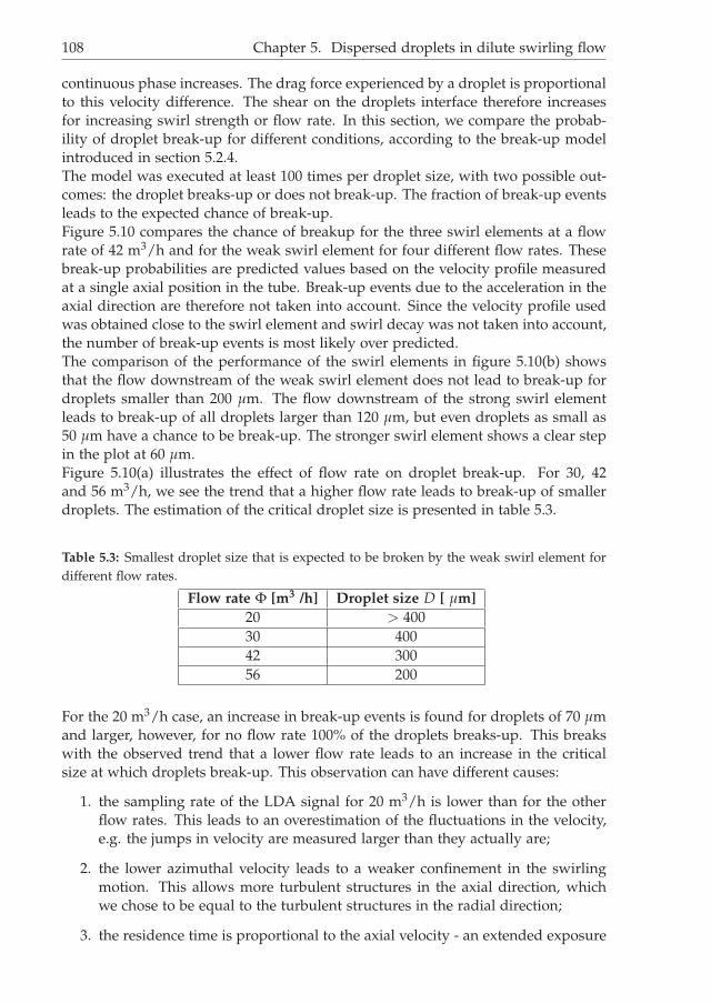
i

i

“Thesis1” — 2014/1/7 — 18:22 — page 108 — #128i

i

i

i

i

i


continuous phase increases. The drag force experienced by a droplet is proportionalto this velocity difference. The shear on the droplets interface therefore increasesfor increasing swirl strength or flow rate. In this section, we compare the probab-ility of droplet break-up for different conditions, according to the break-up modelintroduced in section 5.2.4.The model was executed at least 100 times per droplet size, with two possible out-comes: the droplet breaks-up or does not break-up. The fraction of break-up eventsleads to the expected chance of break-up.Figure 5.10 compares the chance of breakup for the three swirl elements at a flowrate of 42 m3/h and for the weak swirl element for four different flow rates. Thesebreak-up probabilities are predicted values based on the velocity profile measuredat a single axial position in the tube. Break-up events due to the acceleration in theaxial direction are therefore not taken into account. Since the velocity profile usedwas obtained close to the swirl element and swirl decay was not taken into account,the number of break-up events is most likely over predicted.The comparison of the performance of the swirl elements in figure 5.10(b) showsthat the flow downstream of the weak swirl element does not lead to break-up fordroplets smaller than 200 µm. The flow downstream of the strong swirl elementleads to break-up of all droplets larger than 120 µm, but even droplets as small as50 µm have a chance to be break-up. The stronger swirl element shows a clear stepin the plot at 60 µm.Figure 5.10(a) illustrates the effect of flow rate on droplet break-up. For 30, 42and 56 m3/h, we see the trend that a higher flow rate leads to break-up of smallerdroplets. The estimation of the critical droplet size is presented in table 5.3.

Table 5.3: Smallest droplet size that is expected to be broken by the weak swirl element fordifferent flow rates.

Flow rate Φ [m3 /h] Droplet size D [ µm]

20 > 40030 40042 30056 200

For the 20 m3/h case, an increase in break-up events is found for droplets of 70 µmand larger, however, for no flow rate 100% of the droplets breaks-up. This breakswith the observed trend that a lower flow rate leads to an increase in the criticalsize at which droplets break-up. This observation can have different causes:

1. the sampling rate of the LDA signal for 20 m3/h is lower than for the otherflow rates. This leads to an overestimation of the fluctuations in the velocity,e.g. the jumps in velocity are measured larger than they actually are;

2. the lower azimuthal velocity leads to a weaker confinement in the swirlingmotion. This allows more turbulent structures in the axial direction, whichwe chose to be equal to the turbulent structures in the radial direction;

3. the residence time is proportional to the axial velocity - an extended exposure

i

i

“Thesis1” — 2014/1/7 — 18:22 — page 109 — #129i

i

i

i

i

i


20 100 5000

0.1

0.2

0.3

0.4

0.5

0.6

0.7

0.8

0.9

1


chance

ofbre

akup

[−]

20 m3/h

30 m3/h

42 m3/h

56 m3/h

(a) Weak swirl element: four flow rates

20 100 5000

0.1

0.2

0.3

0.4

0.5

0.6

0.7

0.8

0.9

1


chan

ceof

bre

akup

[−]

weak

strong

large


Figure 5.10: Probability for a droplet to break-up during its residence in the cyclone. Eachdatapoint represents at least 100 runs of the model in section 5.2.4. Each model run isdifferent due to the chaotic nature of turbulent velocity measurements.

i

i

“Thesis1” — 2014/1/7 — 18:22 — page 110 — #130i

i

i

i

i

i


to swirling flow promotes break-up.

Interpretation of predicted break-up

The model introduced in this chapter assumes droplets to break when they exceeda critical Weber number, see section 5.2.4. This does not provide information onthe resulting droplet sizes, the so called daughter droplet size distribution. Manymeasurements and models have been developed to provide an accurate descriptionof this distribution. However, the available models show a very wide spread inpredictions of the daughter droplet size distribution [48]. According to the modelintroduced by Martínes-Bazán et al. [49] and validated by Eastwood et al. [50], thedaughter droplet size distribution depends on the turbulent dissipation rate ǫ. Forthe runs of the model in this chapter, we cannot produce an accurate descriptionof the turbulent dissipation. From theory [48, 49], we therefore should assume thedaughter droplets to range in size from almost 0 times the mother droplet to 0.95the diameter of the mother droplet.

5.3.3 Separation window

In the preceding subsections, we obtained both a minimum size of the droplets thatcan be separated and a maximum size before droplets are broken. When dropletsin this range are fed to the cyclone, the optimal separation performance can beexpected.Figure 5.11 compares the time required for a droplet to get to the center of the tube(r/R < 0.2) with the number of break-up events during its path to the center. Thereis a chance of droplet separation when:

• t/T < 1, with t the time to center and T the average residence time of liquidin the cyclone;

• NT/t < 1, with N the total number of break-up events. By dividing thisnumber by the dimensionless time to the center (t/T), we know whether it iscertain that a droplet will break-up (if NT/t > 1) or that a certain number ofdroplets will not be broken. If a droplet is broken, some daughter dropletscan still be within the separation window, but certainly a certain fraction willbe smaller than the lower limit, which reduces the separation efficiency.

The comparison of the three swirl elements (figure 5.11(b)) shows that the abovementioned criterion is not met for the large swirl element. The strong swirl elementhas a small range in which separation is likely: 60 < D < 90 µm and the weakelement has the largest separation window: 70 < D < 200 µm.For the series of calculation in which we varied the flow rate (figure 5.11(a)), table5.4 shows a shift in the separation window.

i

i

“Thesis1” — 2014/1/7 — 18:22 — page 111 — #131i

i

i

i

i

i

5.4. Conclusions 111

Table 5.4: Separation window for the weak swirl element for four different flow rates.

Flow rate Smallest separated Max stable

Φ [m3 /h] size Dmin [ µm] size Dmax [ µm]

20 250 -30 100 35042 70 22056 50 140

5.4 Conclusions

Based on experimental data obtained with Laser Doppler Anemometry, a modelhas been constructed to predict the movement of oil droplets in brine for a verydilute case. The model evaluates the droplet acceleration based on three forces: (i)buoyancy in the centrifugal pressure field, (ii) drag force relative to the surround-ing continuous phase and (iii) the additional inertia due to the acceleration of thesurrounding liquid (added mass) The available velocity information consisted outof time series for the axial and azimuthal velocity. The velocity fluctuations in theaxial directions were used to mimic the velocity fluctuations in the radial direction.Results obtained with the model indicate a range of droplet sizes in which dropletsare likely to be separated with the cyclone:

• droplets smaller than the size at which the droplets will certainly break-up;

• larger than the size at which the turbulent dispersion effect is stronger thanthe acceleration due to the centrifugal motion.

Within this range, there is a window of separation. The daughter droplet sizedistribution following the break-up event has not been considered within this work.Of course, droplets that are too large can break into multiple smaller droplets ofwhich some are still larger than the lower critical size for separation. Based onstatistics from literature, there will certainly be daughter droplets that are too smallto be separated. Therefore, exceeding the maximum droplet size of the separationwindow leads to a reduction in separation quality.For simulations with different flow rates for the same swirl element, the width ofthe window remains of equal order of magnitude. The critical droplet sizes shifts -a lower flow rate leads to an increase in the size of the smallest droplet captured,but also allows larger droplets not being broken up.For tests for three different cyclones at equal flow rate, the width of the separationwindow changed. The weakest swirl element provides the largest window of sep-aration. Stronger swirl elements are likely to separate smaller droplets for a givenflow rate.

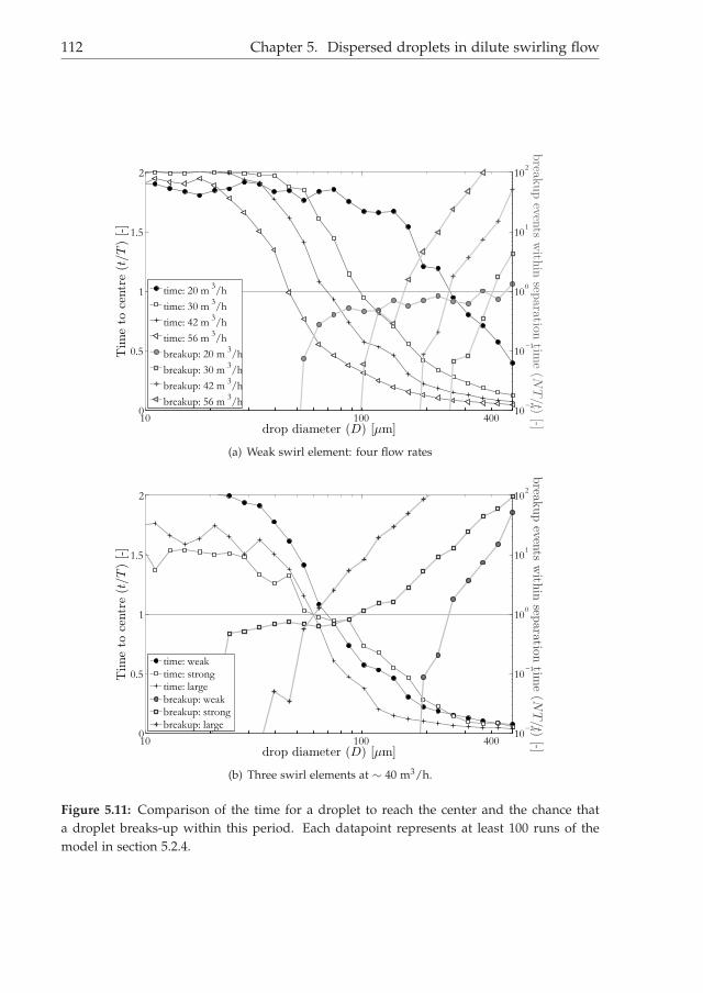
i

i

“Thesis1” — 2014/1/7 — 18:22 — page 112 — #132i

i

i

i

i

i


10 100 4000

0.5

1

1.5

2

drop diameter (D) [µm]

Tim

eto

centr

e(t

/T)

[-]

10-2

10-1

100

101

102

brea

kup

events

with

insep

arationtim

e(N

T/t)

[-]

time: 20 m3/h

time: 30 m3/h

time: 42 m3/h

time: 56 m3/h

breakup: 20 m3/h

breakup: 30 m3/h

breakup: 42 m3/h

breakup: 56 m3/h

(a) Weak swirl element: four flow rates

10 100 4000

0.5

1

1.5

2

drop diameter (D) [µm]

Tim

eto

centr

e(t

/T)

[-]

10-2

10-1

100

101

102

break

up

events

with

insep

arationtim

e(N

T/t)

[-]

time: weak

time: strongtime: large

breakup: weakbreakup: strong

breakup: large


Figure 5.11: Comparison of the time for a droplet to reach the center and the chance thata droplet breaks-up within this period. Each datapoint represents at least 100 runs of themodel in section 5.2.4.

i

i

“Thesis1” — 2014/1/7 — 18:22 — page 113 — #133i

i

i

i

i

i

5.5. Outlook 113

5.5 Outlook

The model in this section is a valuable tool to compare the droplet trajectoriesof Lagrangian simulations with experimental data, since it includes an accuratedescription of turbulent dispersion. As a design tool, it lacks a very importantparameter, namely the droplet break-up due to the acceleration of the liquid. Al-though droplet break-up is extensively discussed in this thesis (chapter 6, it doesnot provide an accurate prediction of the droplet break-up phenomenon, meaningthat we cannot use single phase flow statistics to calculate the droplet size distri-bution downstream of the swirl element. Further insight in the droplet break-upmechanism can be used to improve the model to gain practical separation predic-tions.

i

i

“Thesis1” — 2014/1/7 — 18:22 — page 114 — #134i

i

i

i

i

i

114

i

i

“Thesis1” — 2014/1/7 — 18:22 — page 115 — #135i

i

i

i

i

i

CHAPTER 6

Droplet break-up and coalescence

Two phase liquid-liquid flows can occur in many different flow regimes. The trans-portation at relative high velocities and therewith high Reynolds numbers leads todispersed flow. Shear forces applied on the liquid leads to break-up of droplets,where the overall aim of a separator is to coalesce all dispersed droplets into acontinuous phase.In this chapter, we investigate the droplet break-up and coalescence in the axialcyclones used within this research. The droplet size distribution has been measuredat multiple spots with an intrusive endoscope technique and leads to conclusionson break-up and average coalescence versus break-up behavior. Understanding ofdroplet break-up can be used during the design of cyclones to minimize the dropletsize reduction.

6.1 Droplet size upstream of the swirl element

6.1.1 Turbulent liquid-liquid pipe flow

Turbulent flow is characterized by eddies, ranging in size from the integral scale,down to the Kolmogorov microscale. These eddies exert a force on the dropletthat can break droplets. According to Kolev [36] the droplet size distribution willapproach the size distribution of the smaller turbulent eddies present in the flow.

Hinze model As discusses in chapter 4 Hinze [37] proposed a model for the max-imum droplet size in turbulent flow:

Dmax

(ρc

σ

)3/5ǫ2/5 = 0.725, (6.1)

where ρc is the density of the continuous phase and ǫ the turbulent dissipation rate.The estimation of ǫ is essential for a correct prediction of the maximum dropletsize. The turbulent dissipation rate is connected to the size of the smallest eddies ℓ,which on its turn depends on the microscale to:

115

i

i

“Thesis1” — 2014/1/7 — 18:22 — page 116 — #136i

i

i

i

i

i

116 Chapter 6. Droplet break-up and coalescence

0 50 100 150 200 250 300 350 400 450 5000

0.002

0.004

0.006

0.008

0.01

0.012

0.014

0.016

0.018

0.02

diameter (D) [µm]

volu

met

ric

pdf

10 m3/h

20 m3/h

30 m3/h

40 m3/h

56 m3/h

Figure 6.1: Estimation of the volumetric occupation of the dispersed phase based on dropletphotographs for five different flow rates. Measurements taken at 10 cm upstream of the swirlelement, according to the method in section 3.4.1.

ℓ =

(ν3

ǫ

)1/4

= ℓ0Re−3/4, (6.2)

where ν is the kinematic viscosity and ℓ0 the scale of the biggest eddy (the tubediameter). Taking this into account, the turbulent dissipation rate can be expressedas:

ǫ =ν3Re3

ℓ40

. (6.3)

The relation between flow rate and droplet size was already introduced in chapter4, see figure 4.1. This figure relates the maximum droplet size according to Hinze’smodel (equation 6.1) to the flow rate. At nominal conditions for the flow rig usedin this investigation (56.5 m3/h), the maximum droplet size is predicted to be 234µm. As could be expected, a lower flow rate results in a larger maximum dropletsize.

Experimental data

The theory for the droplet size distribution described above was tested for the turbu-lent multiphase non-swirling pipe flow upstream of the swirl element. The dropletsizes were measured upstream of the swirl element with the intrusive endoscopemethod introduced in section 3.4.1. Figure 6.1 shows the probability of the dropletsizes. The trend for the maximum droplet size in figures 4.1 and 6.1 shows goodagreement.

i

i

“Thesis1” — 2014/1/7 — 18:22 — page 117 — #137i

i

i

i

i

i

6.2. Droplet size reduction with a swirl element 117

6.1.2 Droplet size reduction with valves

Since the droplet size is an important parameter affecting the performance of anaxial cyclone, the need exists to control the droplet size that is fed to the cyclone.The nature of turbulent pipe flow creates a certain droplet size distribution as isdiscussed in the previous section. To reduce the droplet size further, two types ofvalves are used to break droplets with shear: a ball valve and a membrane valve.

Ball valve The ball valve used has a 100 mm inner diameter and a PTFE fitting.The region with high shear is the sharp edge of the port, that can gradually beturned into the flow.Figure 6.2(a) demonstrates the dispersing effect of the ball valve. As an indicationof the additional shear applied to the droplets the pressure drop over the valve isused. The median droplet size at 10 m3/h can be reduced to a median value of 300µm, which is still significantly larger than the droplet size measured at 56.5 m3/h.

Diaphragm valve To reduce the droplet size further than with the ball valve, amembrane valve was used instead. Figure 6.2(b) demonstrates the ability to reducethe droplet size further with a lower pressure drop as compared to the ball valve.Comparing the case at 10 m3/h with 0.56 bar pressure drop over the membranevalve and the 56 m3/h case with no pressure drop, the average droplet size is equal(110 µm). The median differs, since more large droplets are present at the higherflow rate of 56 m3/h.

6.2 Droplet size reduction with a swirl element

6.2.1 Model of the break-up in a swirl element

For most applications, the fluid flow that is accelerated by the swirl element willconsist of dispersed oil droplets in a continuous watery phase. The sphericaldroplets are stretched by the acceleration. Let us assume that the area occupiedby the droplet in a cross-sectional plane remains constant:

D21

A1=

D23

A3, (6.4)

here, D1 is the droplet diameter upstream of the swirl element, A1 is the cross-sectional area of the tube upstream, A3 is the cross-sectional area at the vane tips,where the liquid leaves the swirl element measured in the direction perpendicularto the fluids velocity, and D3 is the droplet diameter in that plane. The indices areillustrated in figure 6.3: 1 is upstream of the swirl element, 2 is at the upstream sideof the vanes and 3 is at the vane tip on the downstream side.The area through which the volume is ejected, A3, is determined by the velocityat the vane tip, governed by the relation A3 = Φ

v3with Φ the flow rate and v3 the

magnitude of the velocity at the vane tip. The first depends on operational settings,the latter on the swirl element of choice. The velocity is discussed in section 4.2.

i

i

“Thesis1” — 2014/1/7 — 18:22 — page 118 — #138i

i

i

i

i

i


0 100 200 300 400 500 600 700 800 900 10000

0.5

1

1.5

2

2.5

3

3.5

4

x 10-3

diameter (D) [µm]

volu

met

ric

pdf

ball 0.1 bar

ball 0.2 bar

ball 0.4 bar

ball 0.6 bar

(a) Ball valve

0 50 100 150 200 250 300 350 4000

0.002

0.004

0.006

0.008

0.01

0.012

0.014

diameter (D) [µm]

volu

met

ric

pdf

diaphragm 0.50 bardiaphragm 0.53 bardiaphragm 0.56 bar

56 m3/h, 0 bar

(b) Membrane valve

Figure 6.2: Volumetric probability density functions (PDFs) of the droplet size distributionsfor two different valves at different valve settings for 10 m3/h at an oil cut of 25 %, comparedwith the droplet size distribution at 56 m3/h without additional shear. Measurement locationwas downstream of the valve and upstream of the swirl element

i

i

“Thesis1” — 2014/1/7 — 18:22 — page 119 — #139i

i

i

i

i

i


12

3

Figure 6.3: Positions at the swirl element used for the estimation of the shear induced break-up.

Since the velocity profile cannot be flat due to wall friction, the effective opening issmaller, like the liquid contraction downstream of an orifice as described by van denAkker and Mudde [44]. We therefore divide this area by 2.The mass and therewith the volume of the droplet, that is stretched by the acceler-ating flow, is conserved. Due to the smaller diameter, the length L of the dropletwill increase. We assume a cylindrical shape with spherical caps:

L =2D3

1 − 2D33

3D23

+ D3, (6.5)

The outer surface of this long droplet is:

Adrop,3 = πLD3 + πD23 (6.6)

The shear force on the droplet is assumed to be equal to the force required toaccelerate the droplet to have the same velocity as the liquid, where the force resultsfrom Newton’s second law, F = m · ∆v/∆t with ∆v = v3 − v2 in the streamwisedirection and ∆t = 2∆s/(v3 + v2). Dividing by the outer surface of the elongateddroplet leads to the shear on the drop:

τ =D3

1ρd

12∆s

v23 − v2

2

LD3 + D23

, (6.7)

with ∆s the length of the vanes along the streamlines. For this shear τ, the Webernumber can easily be calculated according to equation 4.1. The critical Weber num-ber leads to the maximum size of droplets upstream (position 1) that can pass theswirl element intact. Figure 6.4 provides the maximum stable droplet size as func-tion of the flow rate for two different swirl elements: the initial and the weakerelement (see section 4.2). For the nominal conditions of design, 56 m3/h, the max-imum stable droplet size passing the initial swirl element is 0.16 mm and for theweaker swirl element 0.25 mm. Based on this model, we predict that droplets largerthan the respective sizes will break. The resulting size distribution is not predicted

i

i

“Thesis1” — 2014/1/7 — 18:22 — page 120 — #140i

i

i

i

i

i


0 10 20 30 40 50 6010

2

103

0.25 mm

0.16 mm

0.32 mm

1.3 mm

1.4 mm

Flow rate (Φ) [m3/h]

Cri

tica

ldia

met

er(D

crit

)[µ

m]

Weak swirl

Strong swirl

Large swirl

Figure 6.4: Size of the droplets at the critical Weber number in the swirl element for givenflow rate.

using a model. The size will range from a sphere with the diameter D3 (equation6.4) up to a droplet with half of the droplet volume before the break-up event.

6.2.2 Experimental results

Figure 6.5 compares the droplet size downstream of the swirl element for variousinput droplet sizes - the indicated droplet sizes (300, 400 and 500 µm) refer to themedian droplet size obtained with a specific ball valve setting as can be found infigure 6.2(a). The expected critical droplet size is larger than 1 mm for this specificsetting and therefore, we originally did not expect that droplets would be brokenby the swirl element. These results, however, indicate that the mechanism that weintroduced is not complete, effects like shear stress at the wall are neglected in ourmodel.The effect of break-up at 56 m3/h flow was studied for two different swirl elements.Figure 6.6(a) shows that the droplet size is reduced by passing the swirl element.The estimated critical droplet size for the initial swirl element was 0.16 mm and forthe weaker swirl element 0.25 mm. For both elements, the droplet size is reducedto sizes far below this critical size. However, some of the observed droplets arelarger than the predicted maximum size. It could be caused by coalescence justdownstream of the swirl element, since the minimum distance between the swirlelement and the droplet size measurement location was 20 cm.The minimum droplet size observed for the initial swirl element is 4 µm and for theweaker swirl element 10 µm. These diameters are smaller than the diameter of theelongated droplets in the swirl element at the critical Weber number.Figure 6.6(b) compares the droplet size downstream of the swirl element at 10 m3/hfor the weaker and larger swirl element. The size of the droplets in the feed is mostlikely not correct, since the expected droplet size (> 1 mm) does not fit in the field

i

i

“Thesis1” — 2014/1/7 — 18:22 — page 121 — #141i

i

i

i

i

i


0 100 200 300 400 500 600 700 800 900 10000

0.5

1

1.5

2

2.5

3

3.5

4

4.5

5x 10

-3

diameter (D) [µm]

volu

met

ric

pdf

500 µ m

400 µ m

300 µ m

Figure 6.5: Fits of experimentally measured droplet sizes downstream of the weak swirlelement. Three different median droplet sizes in the feed were tested for 10 m3/h at an oilcut of 25 %.

of view of the endoscope and those droplets can therefore not be measured. We seethat the size downstream of the swirl element is very large for the weaker element,some break-up occurs, but the critical size limit of 1.4 mm seems to correspondwith these results. For the larger swirl element, the largest observed droplets aresignificantly smaller than the largest expected droplet size (1.3 mm). This can becaused by the additional shear stress at the wall, since the larger swirl elementcontains much more wall surface than the smaller swirl element.

Trend for droplet size

The theoretical background provided at the beginning of this section deals with themaximum stable droplet size and provides an upper limit for the droplet size. Forpractical purposes, the droplet size of the largest volume fraction is most important,since they represent the largest volume stream that needs to be separated. Themodels discussed in this work do not provide a conclusion on the mean of thevolumetric droplet PDF. Experimental work, however, does provide the medianvalue.Figure 6.7 compares the median of the droplet size as function of the maximum azi-muthal velocity. The graph is composed out of measurements performed for threedifferent swirl elements: the initial swirl element (73), the weaker swirl element(62) and the large diameter swirl element with tapering (equivalent to 73). Basedon the results, it seems that the results of the three swirl elements follow the sametrend. The graph shows a bend at a velocity of about 4 m/s. Below that velocity, themedian of the droplet size is very sensitive for changes in the maximum azimuthal

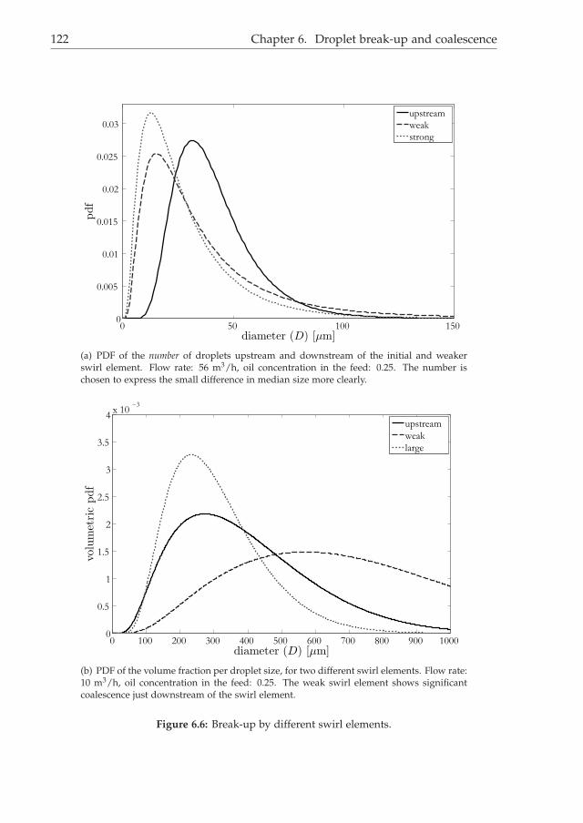
i

i

“Thesis1” — 2014/1/7 — 18:22 — page 122 — #142i

i

i

i

i

i


0 50 100 1500

0.005

0.01

0.015

0.02

0.025

0.03

diameter (D) [µm]

pdf

upstream

weak

strong

(a) PDF of the number of droplets upstream and downstream of the initial and weakerswirl element. Flow rate: 56 m3/h, oil concentration in the feed: 0.25. The number ischosen to express the small difference in median size more clearly.

0 100 200 300 400 500 600 700 800 900 10000

0.5

1

1.5

2

2.5

3

3.5

4x 10

-3

diameter (D) [µm]

volu

met

ric

pdf

upstream

weak

large

(b) PDF of the volume fraction per droplet size, for two different swirl elements. Flow rate:10 m3/h, oil concentration in the feed: 0.25. The weak swirl element shows significantcoalescence just downstream of the swirl element.

Figure 6.6: Break-up by different swirl elements.

i

i

“Thesis1” — 2014/1/7 — 18:22 — page 123 — #143i

i

i

i

i

i

6.3. Droplet coalescence inside the cyclone 123

0 2 4 6 8 10 120

100

200

300

400

500

600

max azimuthal velocity(vθ,m) [m/s]

Dro

ple

tSiz

e(D

)[µ

m]

strong

weak

large

Figure 6.7: Droplet size in the swirling flow as function of the maximum azimuthal velocityin the swirl element for the available droplet sizing datasets. Error bars indicate the standarddeviation in the droplet size distribution function. Solid line indicates fit of equation 6.8.

velocity. For velocities larger than 4 m/s, the sensitivity is smaller and there seemsto be a linear dependence of the median droplet size on the maximum azimuthalvelocity present in the system. The drawn linear fit is:

Dmedian = −8vθ,max + 160 (6.8)

with Dmedian the median droplet size in µm and v the maximum azimuthal velocityin m/s.

6.3 Droplet coalescence inside the cyclone

During their stay in the axial cyclone, droplets will break and coalesce due to theforces caused by the fluid flow. To quantify the net effects, the droplets size distri-bution was measured at four distinct positions in the cyclones, see figure 6.8:

1. upstream of the swirl element;

2. downstream of the swirl element, but upstream of the outlets - the resultsare spatially averaged. The disturbances of the flow pattern do not allow anaccurate measurement of the gradient in droplet size distribution within theswirling flow.

3. in the Heavy Phase Outlet stream, 60 cm downstream of the actual outlet.

4. in the Light Phase Outlet stream, 30 cm downstream of the actual outlet.

i

i

“Thesis1” — 2014/1/7 — 18:22 — page 124 — #144i

i

i

i

i

i


1: Upstream

3: HPO

4: LPO2: swirling fl ow

(spatially averaged)30 cm

60 cm

Figure 6.8: Measurement locations for the endoscope-based droplet sizing method.

Figure 6.9(a) compares the four different positions and leads to the following factualobservations:

• the smallest droplet size downstream of the swirl element is smaller thanupstream of the swirl element.

• downstream of the swirl element there is an increase in the volume fractionof larger droplets

• comparing both outlets, the smaller droplets are more represented in thelighter phase outlet and the larger droplets more in the heavy phase outlet.

The shear in the swirl element will break the droplets, as discussed in section 6.2,this explains why the smallest droplet size downstream of the swirl element issmaller than the smallest droplet size upstream of the swirl element. However,there must also be coalescence events, since the volume of large droplets increases.From the available experimental dataset, we can not conclude where these eventsoccur.Downstream of the swirl element, the fraction of larger droplets increases slightly.This indicates coalescence takes place. Despite the high velocity of the system,different droplets merge to larger ones.Based on the results of chapter 5, we would expect the larger droplets to be presentin the center region at the outlet and the smaller droplets to be spread around overthe complete cross section, leading to a higher fraction large droplets in the LPO.This is different from our experimental results. The difference can be caused bydroplet break-up at the pickup tube wall, or by zones with high shear in the tubebefore measuring the droplets in the LPO. During these measurements, no phaseinversion was observed; phase inversion leads to very bright droplets instead ofdark droplets due to the refractive indices of oil and water.

i

i

“Thesis1” — 2014/1/7 — 18:22 — page 125 — #145i

i

i

i

i

i

6.4. Conclusion 125

Figure 6.9(b) compares the droplet size distribution in the swirling flow regionwith the flow rate-averaged droplet size distribution in both outlets. This averagingprocedure is based on the flow split: 25 % of the LPO distribution plus 75 % of theHPO droplet size distribution. The average droplet size in both outlets is smallerthan the average droplet size in the swirling flow region. Therefore, break-up eventsdominate over coalescence events in the downstream section of the swirltube or atthe beginning of the pickup tube.

6.4 Conclusion

Inlet conditions The droplet size for two-phase turbulent pipe flow is well pre-dictable. We tested the model by Hinze [37] and saw good comparability. Thedroplet sizes upstream of the cyclone can be controlled via two types of valves. Amembrane valve reduces the droplet size stronger than a ball valve, where the ballvalve produces a larger spread than the membrane valve.

Break-up due to swirling flow Droplet break-up in swirling flow can be accoun-ted for by two major effects: (i) acceleration of the liquid at the swirl element and(ii) acceleration of the droplet in the radial direction due to centrifugal buoyancyforces. Theory applied to both effects delivers a maximum droplet size that canwithstand the flow. This maximum size agrees with experimental data reasonably.From experimental data, we derived a relation for the median droplet size Dmedianin µm as function of the maximum azimuthal velocity vθ,max:

Dmedian = −8vθ, max + 160 (6.9)

This relation holds for vθ, max > 4 m/s and can be used to predict the resultingdroplet size distribution when designing a new swirl element. Results are notconclusive what effect causes this break-up, whether the swirl element itself or theswirling flow are the cause.

Outlets In contrast to the concept that larger droplets are more easily acceleratedto the center than smaller droplets, we find that the droplets in the light phase outletare on average smaller than in the heavy phase outlet. For this phenomenon, nosatisfactory explanation has been found.Considering the weighed-averaged droplet size distribution in both outlets, thedroplets are on average smaller in the outlet than just downstream of the swirlelement. This indicates droplet break-up in the swirling flow.

i

i

“Thesis1” — 2014/1/7 — 18:22 — page 126 — #146i

i

i

i

i

i


0 50 100 150 200 250 300 350 4000

1

2

3

4

5

6

7

8

x 10-3

diameter (D) [µm]

volu

met

ric

pdf

upstream

swirl

HPO

LPO

(a) HPO and LPO separate

0 50 100 150 200 250 300 350 4000

1

2

3

4

5

6

7

8

x 10-3

diameter (D) [µm]

volu

met

ric

pdf

upstream

swirl

HPO+LPO

(b) flow rate-averaged sum of the outlets

Figure 6.9: Fits of experimentally measured droplet size distributions for four positions in thecyclone equipped with the weak swirl element: upstream of the swirl element, downstreamof the swirl element in the swirling flow, downstream of the HPO and downstream of theLPO.

i

i

“Thesis1” — 2014/1/7 — 18:22 — page 127 — #147i

i

i

i

i

i

CHAPTER 7

Analysis of swirl separation performance

The preceding chapters 4, 5 and 6 looked at specific parts of the in-line axial cyc-lone to increase understanding. This chapter focuses on the optimization of thegeometry by comparing the separation result for changes in: swirl element, length,pick-up tube diameter. Operational effects are discussed in section 7.2.The method to assess separation efficiency which is used in this chapter is intro-duced in section 3.3.

7.1 Geometric optimization

7.1.1 Swirl element type

The three different swirl elements as used in this research (see section 4.2) werecompared with respect to separation efficiency at their nominal conditions: for thestrong and weak swirl element this is 56 m3/h flow in a 170 cm swirltube with a50 mm pick-up tube. These results are compared with the large swirl element at 30m3/h flow for a 170 cm swirl tube and a 50 mm pick-up tube.Figure 7.1(a) displays the oil concentration in the outlets for the condition that theflow split was kept equal to the oil concentration in the feed. The most significantdifference is found for the region where cin varies between 0.1 and 0.3. The weakswirl element performs best, then the strong swirl element and the large swirl ele-ment shows a relative poor performance. Considering the dispersed efficiency (seeequation 3.10) in figure 7.1(b), the weak swirl element performs better on bulk sep-aration for all conditions. The large swirl element performs for all conditions worsethan the others.Figure 7.1(a) and 7.1(b) also depict numerical separation predictions based on nu-merical simulations by Slot [13]. The Euler-Euler model (see section 3.2) resultsshow a comparable trend for the oil concentration in the outlets: a higher oil cutin the feed leads to more oil in the HPO and less water in the LPO. The predictedseparation is, however, much higher. This can be seen from the dispersed efficiencygraph, where all three numerical data points over predict the lab results. Parameters

127

i

i

“Thesis1” — 2014/1/7 — 18:22 — page 128 — #148i

i

i

i

i

i

128 Chapter 7. Analysis of swirl separation performance

that can cause this wrong predictions are: (i) underestimation of turbulent disper-sion, (ii) the lack of droplet breakup models or (iii) insufficient ensemble-averageddrag relations.

The before mentioned performance difference could have been expected based onresults in figure 5.10(b). In this figure, the window of separation is largest for theweak swirl element (55 - 120 µm), then for the strong swirl element and negligiblefor the large swirl element (around 60 µm). The droplet size distribution fed tothe system is equal for both the strong and weak swirl element. The droplet sizedistribution that enters the large swirl element has a larger average diameter.

Dependence on oil cut

Figure 7.1(a) relates the oil concentration in the feed to the oil concentration in bothoutlets: HPO and LPO. For all swirl elements, the concentration of oil in the HPOrelates severely to the oil concentration in the feed, where up to 10 vol % of oil isremoved. This stream could be further treated in the water treatment system.The Light Phase Outlet (LPO) does not show a proportionality to the oil concentra-tion in the feed. Especially for the weak swirl element, the volumetric oil concentra-tion cout is steady between 0.55 and 0.65 for a range in the feed oil concentration of0.15 to 0.55. No phase inversion in the LPO was observed in this range. This LPOstream is suitable for the oil treatment system.THe large swirl element has a more gradual increase in the LPO cout as function ofthe feed oil cut compared to the weak swirl element. This indicates the necessityfor more processing of its output stream.

Tapering

From LDA measurements in single phase brine, we know that the swirl intensitydecreases over length and therewith the separating force on the droplets decreasesover length. As introduced in section 4.2.4 a reduction in tube diameter in thedownstream direction can be used to increase the azimuthal velocity and therewithto compensate for the reduction of swirl strength due to drag. However, within thisresearch, we use only tapering for the short tube section immediately downstreamof the large swirl element.From this work, we cannot discriminate between the effect of the large swirl ele-ment with less azimuthal acceleration and the relatively rapid tapering. Althoughthe liquid acceleration itself in the taper should not be that large that it can breakdroplets, high shear can occur due to recirculation patterns that might break droplets.Due to the opaque nature of the tube, this phenomenon could not be investigated.The high pressure drop over the combination of large swirl element and taper in-dicates regions with high shear.

7.1.2 Swirl tube length

Separation by an axial cyclone depends in various ways on the length of the swirltube. (i) The residence time in the swirl tube is proportional to its length (ii) The

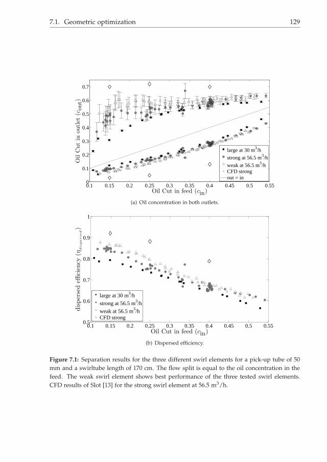
i

i

“Thesis1” — 2014/1/7 — 18:22 — page 129 — #149i

i

i

i

i

i

7.1. Geometric optimization 129

0.1 0.15 0.2 0.25 0.3 0.35 0.4 0.45 0.5 0.550

0.1

0.2

0.3

0.4

0.5

0.6

0.7

Oil Cut in feed (cin)

Oil

Cut

inou

tlet

(cou

t)

large at 30 m3/h

strong at 56.5 m3/h

weak at 56.5 m3/h

CFD strong

out = in

(a) Oil concentration in both outlets.

0.1 0.15 0.2 0.25 0.3 0.35 0.4 0.45 0.5 0.550.5

0.6

0.7

0.8

0.9

1


dis

per

sed

effici

ency

(ηd

isp

er

se

d)

large at 30 m3/h

strong at 56.5 m3/h

weak at 56.5 m3/h

CFD strong

(b) Dispersed efficiency.

Figure 7.1: Separation results for the three different swirl elements for a pick-up tube of 50mm and a swirltube length of 170 cm. The flow split is equal to the oil concentration in thefeed. The weak swirl element shows best performance of the three tested swirl elements.CFD results of Slot [13] for the strong swirl element at 56.5 m3/h.

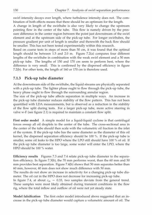
i

i

“Thesis1” — 2014/1/7 — 18:22 — page 130 — #150i

i

i

i

i

i


swirl intensity decays over length, where turbulence intensity does not. The com-bination of both effects means that there should be an optimum for the length.A change in length of the swirltube is also very likely to change the upstreampointing flow in the center of the tube. This flow is namely driven by the pres-sure difference in the center region between the point just downstream of the swirlelement and at the upstream side of the pick-up tube. For longer swirltubes, thepressure gradient per unit of length is smaller and therewith the back flow shouldbe smaller. This has not been tested experimentally within this research.Based on coarse tests in steps of more than 50 cm, it was found that the optimallength should be between 1.5 and 2.0 m. Figure 7.2(a) compares four differentlengths of the swirltube in combination with the weak swirl element and a 50 mmpick-up tube. The lengths of 150 and 170 cm seem to perform best, where thedifference is very small. This is confirmed by the dispersed efficiency in figure7.2(b). For other tests, the length of 160 or 170 cm is therefore used.

7.1.3 Pick-up tube diameter

At the downstream side of the swirltube, the liquid streams are physically separatedwith a pick-up tube. The lighter phase ought to flow through the pick-up tube, theheavy phase ought to flow through the surrounding annular region.The size of the pick-up tube affects separation in multiple ways. An increase inthe pick-up tube diameter reduces stability of the flow pattern. This has not beenquantified with LDA measurements, but is observed as a reduction in the stabilityof the flow split during tests. For a larger pick-up tube, more active steering invalve w-F (see figure 2.1) is required to maintain a constant flow split.

First order model A simple model for a liquid-liquid cyclone is that centrifugalforces sweep all oil droplets to the center of the tube. The cross-sectional area inthe center of the tube should then scale with the volumetric oil fraction in the inletof the system. If the pick-up tube has the same diameter as the diameter of this oilkernel, the dispersed separation efficiency should be 100 %. If the pick-up tube issmaller, some oil leaks to the HPO where the LPO still should have 100 % of oil. Ifthe pick-up tube diameter is too large, some water will enter the LPO, where theHPO should be 100 % water.

Efficiency results Figures 7.3 and 7.4 relate pick-up tube diameter to the separa-tion efficiency. In figure 7.3(b), the 70 mm performs worst, than the 60 mm and 50mm provides best separation. Figure 7.4(b) shows that 50 mm separates better than60 mm, however, 40 mm does not show much difference with 50 mm.The results do not show an increase in selectivity for a changing pick-up tube dia-meter. The oil cut in the HPO does not decrease for increasing pick-up tube.In figure 7.4, at about cin = 0.33, two samples deviate from the general trend.These samples were most likely obtained during transient conditions in the flowrig, where the total inflow and outflow of oil were not yet steady state.

Model falsification The first order model introduced above suggested that an in-crease in the pick-up tube diameter would capture a volumetric amount of oil. The

i

i

“Thesis1” — 2014/1/7 — 18:22 — page 131 — #151i

i

i

i

i

i

7.1. Geometric optimization 131

0.1 0.15 0.2 0.25 0.3 0.35 0.4 0.45 0.5 0.550

0.1

0.2

0.3

0.4

0.5

0.6


Oil

Cut

inou

tlet

(cou

t)

110 cm

150 cm

170 cm

190 cm

out = in


0.1 0.15 0.2 0.25 0.3 0.35 0.4 0.45 0.5 0.550.5

0.6

0.7

0.8

0.9

1


dis

per

sed

effici

ency

(ηd

isp

er

se

d)

110 cm

150 cm

170 cm

190 cm


Figure 7.2: Separation results for the weak swirl element at 56.5 m3/h for four different swirltube lengths, measured from the swirl element tail to the upstream side of the pick-up tube,pick-up tube diameter was 50 mm.

i

i

“Thesis1” — 2014/1/7 — 18:22 — page 132 — #152i

i

i

i

i

i


results do falsify this hypothesis. In contrast, a pick-up tube with a smaller dia-meter leads to a larger oil capture efficiency. An increase in stability of the vortexand therewith of the oil kernel explains this behavior. The optimal situation istherefore such that there is an axial velocity difference between the two outlets.

7.2 Operational optimization

7.2.1 Flow split

For the results presented in section 7.1 a constant flow split was chosen accordingto FS = cin. This choice was made for the simple reason that only for this flowsplit perfect separation can occur: all oil through the LPO and all water throughthe HPO. In this section, we investigate the influence of the flow split on separationperformance.For three different oil concentrations, 0.15, 0.25 and 0.40, the separation efficiencywas determined for a range of flow splits. Figure 7.6(a) shows the dilute efficiency(equation 3.9). This efficiency expresses the amount of oil captured in the LPO. Ascan be easily understood, a higher flow split means more flow through the LPOand therewith a larger part of the total oil flow in the system.The dispersed efficiency (equation 3.10) considers the volumetric liquid flows throughthe “correct” outlets: if all oil runs through the LPO and all water through the HPO,the dispersed efficiency is 100 %. Figure 7.6(b) shows the general trend that a smal-ler flow split leads to a higher dispersed efficiency. Considering figure 7.5 we seemainly an increase in the oil concentration for the LPO for smaller flow split. Themaximum dispersed efficiency is obtained for all cases where the flow split is smal-ler than or equal to the oil concentration in the feed. In figure 7.6(b) this region isindicated with a dashed line. Reduction of the flow split below cin is not profitable,therefore FS = cin seems optimal for most applications.Numerical results by Slot [13] with the Euler-Euler model (see section 3.2) show thesame trend for both the dilute and dispersed efficiency. The efficiency is, however,over predicted for all cases. Parameters that can cause this wrong predictions are:(i) underestimation of turbulent dispersion, (ii) the lack of droplet breakup modelsor (iii) insufficient ensemble-averaged drag relations.

Different swirl elements The hypothesis that the optimum for the dispersed ef-ficiency is reached for the condition FS = cin was tested for the strong and weakswirl element. Figure 7.7 compares the strong and weak swirl element for an oilcut of 25 % in the feed. We see that the trend is comparable, where the weak swirlelement obtains a slightly higher efficiency.

Different droplet sizes Figure 7.8 compares the efficiency as function of the flowsplit for two different input cases: (i) 10 m3/h with 10 % oil dispersed in dropletswith a mean diameter of over 500 µm and (ii) 10 m3/h with 25 % oil dispersed indroplets with a mean diameter of 100 µm.

i

i

“Thesis1” — 2014/1/7 — 18:22 — page 133 — #153i

i

i

i

i

i

7.2. Operational optimization 133

0.1 0.15 0.2 0.25 0.3 0.35 0.4 0.45 0.5 0.55 0.60

0.1

0.2

0.3

0.4

0.5

0.6


Oil

Cut

inou

tlet

(cou

t)

50 mm

60 mm

70 mm

out = in


0.1 0.15 0.2 0.25 0.3 0.35 0.4 0.45 0.5 0.55 0.60.5

0.55

0.6

0.65

0.7

0.75

0.8

0.85

0.9


dis

per

sed

effici

ency

(ηd

isp

er

se

d)

50 mm

60 mm

70 mm

(b) Dispersed efficiency

Figure 7.3: Separation results for the weak swirl element at 56.5 m3/h for three differentpick-up tube diameters, for a swirltube length of 170cm.

i

i

“Thesis1” — 2014/1/7 — 18:22 — page 134 — #154i

i

i

i

i

i


0.1 0.15 0.2 0.25 0.3 0.35 0.4 0.45 0.5 0.55 0.60

0.1

0.2

0.3

0.4

0.5

0.6


Oil

Cut

inou

tlet

(cou

t)

40 mm

50 mm

60 mm

out = in


0.1 0.15 0.2 0.25 0.3 0.35 0.4 0.45 0.5 0.55 0.60.5

0.55

0.6

0.65

0.7

0.75

0.8

0.85

0.9


dis

per

sed

effici

ency

(ηd

isp

er

se

d)

40 mm

50 mm

60 mm


Figure 7.4: Separation results for the strong swirl element at 56.5 m3/h for three differentpick-up tube diameters, for a swirltube length of 170cm.

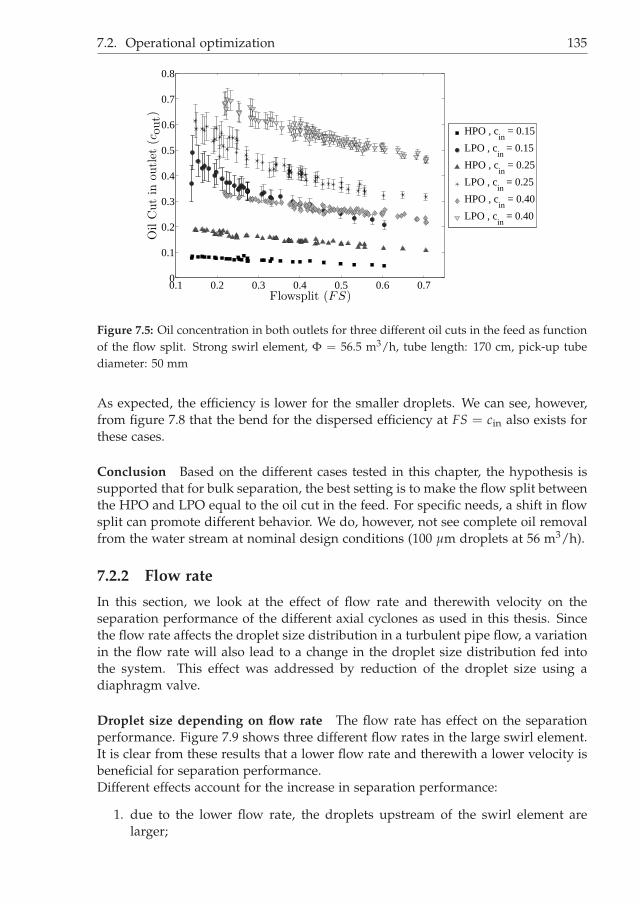
i

i

“Thesis1” — 2014/1/7 — 18:22 — page 135 — #155i

i

i

i

i

i


0.1 0.2 0.3 0.4 0.5 0.6 0.70

0.1

0.2

0.3

0.4

0.5

0.6

0.7

0.8

Flowsplit (FS)

Oil

Cut

inoutl

et(c

out)

HPO , cin

= 0.15

LPO , cin

= 0.15

HPO , cin

= 0.25

LPO , cin

= 0.25

HPO , cin

= 0.40

LPO , cin

= 0.40

Figure 7.5: Oil concentration in both outlets for three different oil cuts in the feed as functionof the flow split. Strong swirl element, Φ = 56.5 m3/h, tube length: 170 cm, pick-up tubediameter: 50 mm

As expected, the efficiency is lower for the smaller droplets. We can see, however,from figure 7.8 that the bend for the dispersed efficiency at FS = cin also exists forthese cases.

Conclusion Based on the different cases tested in this chapter, the hypothesis issupported that for bulk separation, the best setting is to make the flow split betweenthe HPO and LPO equal to the oil cut in the feed. For specific needs, a shift in flowsplit can promote different behavior. We do, however, not see complete oil removalfrom the water stream at nominal design conditions (100 µm droplets at 56 m3/h).

7.2.2 Flow rate

In this section, we look at the effect of flow rate and therewith velocity on theseparation performance of the different axial cyclones as used in this thesis. Sincethe flow rate affects the droplet size distribution in a turbulent pipe flow, a variationin the flow rate will also lead to a change in the droplet size distribution fed intothe system. This effect was addressed by reduction of the droplet size using adiaphragm valve.

Droplet size depending on flow rate The flow rate has effect on the separationperformance. Figure 7.9 shows three different flow rates in the large swirl element.It is clear from these results that a lower flow rate and therewith a lower velocity isbeneficial for separation performance.Different effects account for the increase in separation performance:

1. due to the lower flow rate, the droplets upstream of the swirl element arelarger;

i

i

“Thesis1” — 2014/1/7 — 18:22 — page 136 — #156i

i

i

i

i

i


0.1 0.2 0.3 0.4 0.5 0.6 0.7

0.4

0.5

0.6

0.7

0.8

0.9

1

Flowsplit (FS)

Dilute

effici

ency

(ηd

ilu

te)

cin

= 0.15

cin

= 0.25

cin

= 0.40

CFD cin

= 0.25

(a) Dilute efficiency.

0.1 0.2 0.3 0.4 0.5 0.6 0.70.45

0.5

0.55

0.6

0.65

0.7

0.75

0.8

0.85

0.9

Flowsplit (FS)

Dis

per

sed

effici

ency

(ηd

isp

er

se

d)

cin

= 0.15

cin

= 0.25

cin

= 0.40

CFD cin

= 0.25


Figure 7.6: Separation results as function of the flow split for the strong swirl element. Φ =

56.5 m3/h, three different oil cuts in the feed, tube length: 170 cm, pick-up tube diameter: 50mm. Numerical results by Slot [13].

i

i

“Thesis1” — 2014/1/7 — 18:22 — page 137 — #157i

i

i

i

i

i


0.1 0.2 0.3 0.4 0.5 0.6 0.7 0.80.2

0.3

0.4

0.5

0.6

0.7

0.8

0.9

1

Flowsplit (FS)

Effi

cien

cy(η

)

ηdilute

strong element

ηdilute

weak element

ηdispersed

strong element

ηdispersed

weak element

Figure 7.7: Separation results as function of the flow split for the strong and weak swirlelement. Φ = 56.5 m3/h, cin = 0.25 tube length: 170 cm, pick-up tube diameter: 50 mm.

2. the lower axial velocity leads to a lower velocity along the vanes of the swirlelement and a lower azimuthal velocity in the swirltube. Therewith, thedroplet breakup during the swirl generation is reduced;

3. the centrifugal acceleration of dispersed droplets is reduced due to the lowerazimuthal velocity.

Considering figure 5.11(a), we see that a lower flow rate shifts the window of separ-ation towards larger droplets. This graph does not consider the larger droplet sizesupstream caused by the lower flow rate. From the observations presented in thissection, we learn that for a decreasing flow rate, the average droplet size upstreamincreases more than the shift of the separation window, being beneficial for separa-tion performance. For a low flow rate, the droplets downstream of the swirl elementare larger compared to a high flow rate. Due to the proportionality of the drag forcewith surface (D2

d) and of the centrifugal buoyancy force with volume (D3d), we easily

see the advantage of larger droplets, even at a lower azimuthal velocity.

Constant droplet size In the previous section 7.2.2, we saw that a lower flow rateleads to larger droplets upstream and that it is beneficial on separation behavior.For liquid-liquid flows, the separation equipment should not reduce the dropletsize below the droplet size of the feed, since larger droplets tend to separate moreeasily than smaller droplets.To study the effect of flow rate with constant droplet size, a membrane valve wasused to reduce the droplets upstream of the swirl element at lower flow rates. Sec-tion 6.1.2 shows the resulting droplet size distributions fed to the swirl element.Figure 7.10 shows the separation behavior at three different flow rates where thedroplets sizes are on average equally sized at 100 µm. Due to the differences in the

i

i

“Thesis1” — 2014/1/7 — 18:22 — page 138 — #158i

i

i

i

i

i


0 0.1 0.2 0.3 0.4 0.5 0.6 0.7 0.8 0.9 10.1

0.2

0.3

0.4

0.5

0.6

0.7

0.8

0.9

1

Flowsplit (FS)

Effi

cien

cy(η

)

ηdilute

for cin

= 0.10, > 500 µ m

ηdilute

for cin

= 0.25, 100 µ m

ηdispersed

for cin

= 0.10, > 500 µ m

ηdispersed

for cin

= 0.25, 100 µ m

Figure 7.8: Separation results as function of the flow split for the large swirl element. Φ = 10m3/h, tube length: 160 cm, pick-up tube diameter: 50 mm. A case with 10 vol. % oil andlarge droplets is compared with 25 vol.% oil and 100 µm droplets.

breakup for the various flow rates, the droplet size distributions are different (seesection 6.1.2).The droplets of 100 µm are broken at the swirl element at 56 m3/h to about 60 µmon average. For 10 m3/h and 40 m3/h they are hardly broken and remain at 100µm. In graph 7.10 we can therefore make two comparisons:

• Effect of azimuthal velocity on separation for constant droplet size down-stream of the swirl element (10 m3/h vs 40 m3/h). For the 40 m3/h, there isa small increase in separation over the 10 m3/h case.

• Effect of azimuthal velocity on separation for known difference in droplet sizedownstream of the swirl element (100 µm for 40 m3/h vs 60 µm for 56.5m3h). The centrifugal accelerating body force per unit of volume increaseswith a factor of (56.5/40)2 = 2, where the average drag per unit of volumeincreases with 100/60 = 1.7. Based on this order of magnitude comparison,the separation for 56.5 m3/h should not be significantly improved over 40m3/h, which is in contrast with observations.

Conclusion If the upstream velocity of the liquid-liquid flow is low and the flowregime contains large dispersed droplets or liquid chunks, a lower flow rate andtherewith centrifugal acceleration is preferred, at least within the operational bound-aries used within this research.

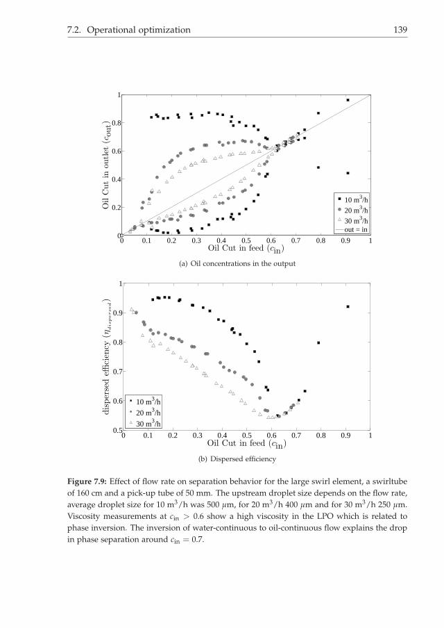
i

i

“Thesis1” — 2014/1/7 — 18:22 — page 139 — #159i

i

i

i

i

i


0 0.1 0.2 0.3 0.4 0.5 0.6 0.7 0.8 0.9 10

0.2

0.4

0.6

0.8

1


Oil

Cut

inou

tlet

(cou

t)

10 m3/h

20 m3/h

30 m3/h

out = in

(a) Oil concentrations in the output

0 0.1 0.2 0.3 0.4 0.5 0.6 0.7 0.8 0.9 10.5

0.6

0.7

0.8

0.9

1


dis

per

sed

effici

ency

(ηd

isp

er

se

d)

10 m3/h

20 m3/h

30 m3/h


Figure 7.9: Effect of flow rate on separation behavior for the large swirl element, a swirltubeof 160 cm and a pick-up tube of 50 mm. The upstream droplet size depends on the flow rate,average droplet size for 10 m3/h was 500 µm, for 20 m3/h 400 µm and for 30 m3/h 250 µm.Viscosity measurements at cin > 0.6 show a high viscosity in the LPO which is related tophase inversion. The inversion of water-continuous to oil-continuous flow explains the dropin phase separation around cin = 0.7.

i

i

“Thesis1” — 2014/1/7 — 18:22 — page 140 — #160i

i

i

i

i

i


0 0.1 0.2 0.3 0.4 0.5 0.6 0.7 0.8 0.9 10

0.2

0.4

0.6

0.8

1


Oil

Cut

inou

tlet

(cou

t)

10 m3/h

40 m3/h

56.5 m3/h

out = in


0 0.1 0.2 0.3 0.4 0.5 0.6 0.7 0.8 0.9 10.5

0.6

0.7

0.8

0.9

1


dis

per

sed

effici

ency

(ηd

isp

er

se

d)

10 m3/h

40 m3/h

56.5 m3/h


Figure 7.10: Effect of flow rate on separation behavior for the weak swirl element, a swirltubeof 160 cm and a pick-up tube of 50 mm. The upstream droplet size were kept approximatelyconstant at 100 µm.

i

i

“Thesis1” — 2014/1/7 — 18:22 — page 141 — #161i

i

i

i

i

i


For small droplets fed to the cyclone, best separation performance is obtained at amaximum azimuthal velocity, as long as the droplet size is not reduced significantly.

The optimal azimuthal velocity for separation seems to be that velocity where thedroplet size to which the droplets are broken is equal to the droplet size upstream.This hypothesis was tested for a limited range of cases as was available within thisresearch.

• For a constant droplet size with a mean of 100 µm, we see that an increase inswirling velocity is favorable.

• For 56.5 m3/h flow, we see an increase in performance for a reduction of swirlstrength, see figure 7.1(a). The feed consists out of average 100 µm droplets,the strong swirl element reduces droplets at the given flow rate to 40 µm, theweak swirl element to 60 µm. No swirl element was available with a dropletsize reduction to 100 µm at the given flow rate.

It is best to operate at a flow rate which corresponds to the droplet size producedby that specific flow rate.

7.2.3 Droplet size

In the previous section (7.2.2) we saw that the droplet size distribution has a sig-nificant effect on separation performance. Turbulent dispersion breaks droplets inpipe flow (see section 6.1.1), which puts a maximum at the droplet size for givenflow rate. To study the effect of droplet size on separation, we measured the separ-ation performance for the lowest flow rate used in this work (10 m3/h) for dropletswith a median size of 100, 300 and 500 µm.Figure 7.11 shows the huge effect on separation. For a flow rate of 10 m3/h, theweak swirl element does not significantly breaks droplets of 500 µm and smaller(chapter 6, figure 6.5). This graph illustrates the need to avoid droplet breakup asmuch as possible, since smaller droplets are harder to separate than larger droplets.

7.2.4 Phase inversion

During the tests, such as in figure 7.9 the oil cut in the flow was varied between0.05 and 0.9. The dispersed efficiency curve has a dip around cin = 0.55 and theoil concentration in HPO and LPO is almost equal for the region where cin rangesbetween 0.55 and 0.8.The most likely explanation for this dip in performance in the indicated region isphase inversion, where (a part of) the dispersed system converts from an oil-in-water emulsion to a water-in-oil emulsion, the structure of the fluids changes. Oneof the observed effects is a peak in viscosity and a step in the electrical conductivityof the liquid.In this research, we measured the viscosity with an Endress+Hauser Promass 83ICoriolis flow meter in the LPO, which measures the fluids response to a torsionalmoment. Since a dispersed two-phase system does not necessarily behave like aNewtonian fluid, the viscosity measurement will be off with an unknown factor.However, it is certain that there is a certain proportionality.

i

i

“Thesis1” — 2014/1/7 — 18:22 — page 142 — #162i

i

i

i

i

i


0 0.1 0.2 0.3 0.4 0.5 0.6 0.7 0.8 0.9 10

0.2

0.4

0.6

0.8

1


Oil

Cut

inou

tlet

(cou

t)

500 mu

300 mu

100 mu

out = in


0 0.1 0.2 0.3 0.4 0.5 0.6 0.7 0.8 0.9 1

0.5

0.6

0.7

0.8

0.9

1


dis

per

sed

effici

ency

(ηd

isp

er

se

d)

500 mu

300 mu

100 mu


Figure 7.11: Effect of droplet size on separation behavior for the weak swirl element, aswirltube of 160 cm, a pick-up tube of 50 mm and a flow rate of 10 m3/h. The upstreamdroplet size were reduced with a membrane valve to a distribution with the median indicatedin the figure. The flow split was equal to the oil concentration in the feed. Large dropletsyield a higher separation performance.

i

i

“Thesis1” — 2014/1/7 — 18:22 — page 143 — #163i

i

i

i

i

i


0 0.2 0.4 0.6 0.8 10

5

10

15

20

25

30

35

40

45


Rel

ati

veK

inem

ati

cV

isco

sity

(η/η w

)

10 m3/h

20 m3/h

Figure 7.12: Measured viscosity of the mixture in the LPO as function of the oil cut attwo different flow rates. Weak swirl element, 160 cm swirltube and 40 mm pick-up tube.The Flow split was chosen to be equal to the oil cut. Measurements are normalized usingthe measured viscosity of pure brine. No compensation has been applied for errors in themethod of measurement in the Endress+Hauser Promass 83I.

Viscosity at the inversion point Figure 7.12 shows the normalized data for thekinematic viscosity in the LPO. The measured values were divided by the meas-ured value for pure brine. Two different flow rates are compared. The graph showsa steeper increase as function of the oil cut for the higher (20 m3/h) flow rate com-pared to the lower (10 m3/h) flow rate. This can be caused by the smaller dropletscreated at higher velocities, where smaller droplets introduce more apparent vis-cosity.For both cases, the viscosity peaks at an oil cut of 0.66 up to a measured valueof 40 times the viscosity of brine. This should therefore be the point at which thephase inversion is occurring. During normal operation of a cyclone, one shouldavoid operation at these conditions, since they hamper separation, leaving the axialcyclone as mixing-only device.The reason why the separation holds back at the phase inversion point is two fold:

1. The high viscosity dampens the swirling motion and therewith the centrifugalacceleration.

2. The drag of droplets moving in the radial direction is proportion to the liquidviscosity. A high viscosity leads to a lower separation quality.

As a consequence above a critical viscosity of the mixture, no separation is expected.This threshold at which separation stops seems to be a viscosity in the order of 20times the viscosity of brine.

i

i

“Thesis1” — 2014/1/7 — 18:22 — page 144 — #164i

i

i

i

i

i


7.3 Static versus Rotating element

This section provides results obtained with a rotating swirl element - in a differentflow rig than used for the rest of the work in this thesis. Details on this flow rigcan be found in section 2.6. The following differences between the rotating swirlelement rig and the rest of the work described in this thesis are found:

• Tube diameter: 50 mm for the rotating swirl element vs 100 mm for the staticswirl element. The linear upstream velocities were matched.

• Droplet size: the droplet size distribution upstream was not measured for therotating swirl element. From the colour of the mixture, the expectation is thatthe droplet size distribution had a larger average size for the rotating swirlelement than for the static swirl element.

• Swirl strength: The swirl number generated by the rotating swirl element isnot known. The velocity of the impeller tips is 7 m/s in the 50 mm tube.However, the slip between the impeller and the liquid is not predicted withinthe scope of the present research. Based on figure 6.7, we can be sure thatthis results into less droplet breakup than the static swirl element at 12 m/s.Further work could consider propulsion theory (of ships and aircrafts).

Figure 7.13 demonstrates better separation performance for the rotating swirl ele-ment. As mentioned above, conditions are not equal. Apparently, the movingnature of the rotating swirl element does not seem to introduce additional dropletbreakup. Furthermore, we see that a lower azimuthal velocity in the swirl regionis beneficial for separation performance. A smaller diameter reduces the distancerequired for a droplet to get separated. This effect is also advantageous for the testswith a rotating swirl element.

7.4 Conclusion

In this chapter, we compared the separation efficiency for different designs anddifferent conditions of our in-line axial cyclone. If the flow rate and droplet sizedistribution are constant, then the design of the swirl element has most influence.The effect of the swirl element on separation performance is likely to be caused bythe droplet breakup that occurs in the swirl element. The length of the swirl sectionhas a relative mild effect on the separation quality, with an optimum in this researchof a length L/D = 16. For the diameter of the pick-up tube, it seems that a smallersize is favorable within the range Dpu/D from 0.4 to 0.7.

During the operation of the cyclone, especially the fluid velocity has a large in-fluence on separation performance. The origin of this strong correlation is dropletbreakup, caused by the shear exerted on the droplets interface, as is explained insection 4.1. Figure 6.7 shows the correlation between the maximum velocity present

i

i

“Thesis1” — 2014/1/7 — 18:22 — page 145 — #165i

i

i

i

i

i

7.4. Conclusion 145

0 0.05 0.1 0.15 0.2 0.25 0.3 0.35 0.4 0.45 0.50

0.1

0.2

0.3

0.4

0.5

0.6

0.7

0.8


Oil

Cut

inou

tlet

(cou

t)

Rotating

Static Stronger

out = in

Figure 7.13: Oil concentration in both outlets for a rotating swirl element (impeller) and astatic swirl element (strong swirl element of this work). The impeller was operated at 50 Hz(maximum frequency) in a 17 m3/h flow in a 50 mm tube with 21 mm diameter pick-uptube. The static swirl element was operated at 56.5 m3/h in a 100 mm tube with a length of160 cm and a pick-up tube of 50 mm diameter.

in the system and the resulting droplet size distribution. From the work in section7.2.2 we learn that for given droplet size distribution, the separation performanceincreases with decreasing azimuthal velocity, until the azimuthal velocity is suchthat the droplets are not broken anymore by the swirl element. The optimal axialcyclone therefore breaks droplets down to the size in the feed, or actually, is de-signed such that there is just no droplet breakup. We should keep in mind that thedroplet size distribution is not necessarily known for producing oil wells.

i

i

“Thesis1” — 2014/1/7 — 18:22 — page 146 — #166i

i

i

i

i

i

146

i

i

“Thesis1” — 2014/1/7 — 18:22 — page 147 — #167i

i

i

i

i

i

CHAPTER 8

Design considerations for Liquid-Liquid

Cyclones

The aim of the research presented in this thesis is the development of understand-ing of in-line axial cyclones for bulk oil/water separation. Although a thorough un-derstanding of the dispersed, multiphase, turbulent and swirling flow is requiredto know what to change in the design, current research progress does not allowan easy, full-scale numerical simulation nor an exact theoretical prediction. In thedesign process of liquid-liquid cyclones, a solution to the design challenge is relyingon non-dimensional scaling of cyclone separation performance data. Therefore, thisconcluding chapter provides basic guidelines on the optimization of cyclone designbased on non-dimensional numbers.

8.1 Scaling parameters

Within this research, we limited ourselves to three different cyclones with a limitedrange of flow rates, and only a single oil/water system. By proper non-dimensionalscaling, the results can be extended to more generic cases.

Efficiency To compare efficiency, the bulk efficiency as introduced in equation 3.11is used:

ηbulk =cin − cHPO

2cin+

cLPO − cin

2 − 2cin. (8.1)

The bulk efficiency is 0 when the oil concentrations in the output are equal to theoil concentration in the input and 1 when only oil flows through the LPO and onlywater through the HPO.

8.1.1 Reynolds number

The Reynolds number compares the inertial forces and viscous forces. The mediandroplet size downstream of the swirl element is related to the Reynolds number,

147

i

i

“Thesis1” — 2014/1/7 — 18:22 — page 148 — #168i

i

i

i

i

i

148 Chapter 8. Design considerations for Liquid-Liquid Cyclones

which we calculate based on the azimuthal velocity and downstream droplet dia-meter:

Reθ =vθ Ddownstream

νc(8.2)

Figure 8.1 relates the swirling Reynolds number (eq. 8.2) to the bulk efficiency (eq.8.1). The different measurement points represent different settings in the flow rig:three different swirl elements, a range of flow rates and a range of droplet sizes. Allsamples were obtained for a swirltube with a length of about 170 cm and a pickuptube diameter of 40 or 50 mm. Both the oil cut in the feed and the flow split were0.25.From the results, we observe the trend that the highest obtained efficiency is largerfor higher Reθ . The Reynolds number balances inertial forces against viscous forces.When viscous forces dominate, the droplet is easily dispersed by turbulent eddies.When inertial forces dominate, the droplet will move according to the centrifugalbuoyancy force and get separated. Based on this theory and the measurementdata in figure 8.1, a linear relation for the maximum obtainable efficiency ηbulk issuggested as function of Reθ .

8.1.2 Weber number

The Weber number expresses the balance between the shear forces that tear adroplet apart and the interfacial tension force that holds the droplet together:

We =

∣∣~t∣∣ D2

σD. (8.3)

For an axial cyclone, the location with the highest velocity is the annular gap of theswirl element: the droplets that have an upstream diameter Dupstream are exposed tothe high azimuthal velocity generated in the swirl element. The acceleration of thedroplets to this high velocity applies a force on their surface which leads to a Webernumber of the form:

We =ρdv2

θ Dupstream

σ(8.4)

Figure 8.2 relates the Weber number (eq. 8.4) to the bulk efficiency (eq. 8.1). Themeasurement points are the same as used in figure 8.1, as described in the previousparagraph on the Reynolds number results.From the results, we observe the trend that the highest obtained efficiency is largerfor lower We. The Weber number relates the shear forces caused by the dropletacceleration in the swirl element to the interfacial tension force that holds thedroplet together. A lower Weber number therefore means that the droplets aremore stable when passing the swirling flow. Unstable droplets break, leading tosmaller droplets that are harder to separate.Similar to the figure with the Re-number results, we draw a suggested line thatrepresents maximum separation as function of the Weber number. Although wecannot exclude the possibility of cases where this line is exceeded, the line seems to

i

i

“Thesis1” — 2014/1/7 — 18:22 — page 149 — #169i

i

i

i

i

i

8.2. Prediction of current swirl elements 149

be a feasible maximum. An interesting property of the fit is that it predicts ηbulk = 1for We = 0.

8.2 Prediction of current swirl elements

Based on the experimental data for the three different swirl elements describedin this thesis (see chapter 4), we can relate the Weber and Reynolds number forthe behavior in the Delft flow rig used for this work, meaning that the interfacialtension and liquid densities of the experiments in this thesis are used (σ = 30mN/m, ρd = 872 kg/m3 and ρc = 1064 kg/m3).

8.2.1 Method

For each flow rate, the droplet size upstream was calculated, according to an expo-nential relation fitted through the maxima of figure 6.1:

D = 836e−1.04u [µm], (8.5)

with u the continuous phase velocity containing the droplets and with a maximumdroplet size of 500 µm.The flow rate is directly coupled to the azimuthal velocity in each swirl elementand the relations between flow rate and azimuthal velocity as derived from theLDA measurement data found in chapter 4:

uθ =

5.0ub strong swirlelement3.5ub weak swirlelement7.0ub large swirlelement

. (8.6)

The value of uθ is used for both the We as Reθ number. The droplet sizes down-stream of the swirl element are calculated according to equation 8.5 for the azi-muthal velocity downstream of the swirl element (eq. 8.6.

The set of equations is evaluated for a range of flow rates, from 0.5 to 80 m3/h.Each flow rate combined with a swirl element results in a Weber number upstreamand a Reynolds number downstream as in figure 8.3.

8.2.2 Reynolds depends on Weber

Figure 8.3 shows the relation for the three swirl elements between Reθ and We.Due to the common rules used in the method of section 8.2.1 and the link betweenthe flow rate and azimuthal velocities, the curves coincide almost. The kink inthe curve at We ≈ 10 is caused by the restriction that droplets are not larger than500 µm. Actual measurements are plotted as dots in figure 8.3. For some cases,the droplet size is reduced with a membrane valve (see section 7.2.3) leading to adecrease in both We as Reθ number. All performed tests follow more or less thepredicted curve for Reθ (We).

i

i

“Thesis1” — 2014/1/7 — 18:22 — page 150 — #170i

i

i

i

i

i


0 100 200 300 400 500 600 700 800 900 10000

0.1

0.2

0.3

0.4

0.5

0.6

0.7

0.8

0.9

1

1

2

3

4

5

6

7

8

9

10

11

Reθ =Dd,DSvθ

νc

Bulk

effici

ency

(ηbu

lk)

Strong

Weak

Large

CFD strong

Figure 8.1: Separation efficiency as function of the droplets Reynolds number (eq. 8.2).Error bars indicate the non-dimensionalized median of the droplet size in swirling flow, datapoints are number as in figure 8.2. CFD results for the strong swirl element by Slot [13].There seems to be a maximum separation for each Reynolds number; a linear function isplotted to represent this possible maximum. This seems feasible, since more droplet inertiamakes it less vulnerable to turbulent dispersion.

We =ρdv

2

θDd,US

σ

Bulk

effici

ency

(ηbu

lk)

Figure 8.2: Separation efficiency as function of the Weber number of the median droplet sizeat the maximum azimuthal velocity in the swirl element. Error bars indicate the droplet sizedownstream of the swirl element, data points are number as in figure 8.1. CFD results forthe strong swirl element by Slot [13]. There seems to be a maximum separation efficiency, avisual exponential decay. A lower Weber number enables a higher separation efficiency.

i

i

“Thesis1” — 2014/1/7 — 18:22 — page 151 — #171i

i

i

i

i

i

8.3. Guide on cyclone design 151

8.2.3 Optimal point of operation

Measured separation efficiency results show a dependency on the Reθ and We num-ber. A high Reθ is favorable for separation, where a high We works counter effectiveon separation. We should therefore operate an in-line axial cyclone at a point wherewe have a high Reθ and a low We. From figure 8.3 we see that the azimuthal ve-locity couples the Reynolds and Weber number and that the swirl element designitself cannot significantly change this.From the suggested maximum bulk efficiency in figures 8.1 and 8.2, we obtain thefollowing relations:

ηbulk, max = a1Reθ + b1 ∝ c1vθ + d1 (8.7)

ηbulk, max = −a2We + b2 ∝ c2v2θ + d2, (8.8)

with a, b, c and d constants. Due to the quadratic nature of equation 8.8 and thelinear behavior of 8.7, a higher azimuthal velocity is not beneficial for separation. Infigure 8.3, we see that the maximum value for Reθ is obtained at a low We number.This is, again, caused by the upper limit for the droplet size of 500 µm.

Numerical results In chapter 7, we saw an over prediction of separation perform-ance in the numerical simulations done by Slot [13]. In figure 8.3, many measure-ment points for the CFD work are above the predicted lines based on the work inthis thesis. Cause is the lack of droplet breakup in some of the numerical datasets;a consequence is an over prediction of separation.

8.2.4 Dependence on droplet size

The curve in figure 8.3 shows a kink. Where the droplet size upstream of the cyc-lone depends on the velocity according to Hinze’s theory, we imposed a maximumof 500 µm: beyond this level, the dispersed phase does not behave like dropletsanymore. The same curve has been computed with smaller maximum upstreamdroplet sizes: 100, 200, 300 and 400 µm. Figure 8.4 shows the Reθ-We-plots forthose conditions. For these smaller droplets, the peak in Reθ shifts to a larger valueof We. This translates to a cyclone with a higher azimuthal velocity that obtains themaximum possible efficiency for given Weber number. The graph does not predictthe efficiency at that specific point.A remarkable observation from figure 8.4 is the splendid resemblance of the modeland measurement data for the 100 µm droplets.

8.3 Guide on cyclone design

From section 8.2 and previous chapters in this thesis, we know the importancefor cyclones of droplet break up in relation to the azimuthal velocity. This sectionprovides a guide on the design of cyclones considering the optimal balance between

i

i

“Thesis1” — 2014/1/7 — 18:22 — page 152 — #172i

i

i

i

i

i


We =D

d,USv2

θρd

σ

Re

θ=

vθD

d,D

S

νc

Figure 8.3: Weber and Reynolds number of figures 8.1 and 8.2. The theoretical relation foreach swirl element is depicted, and actual measurement results. The coupling between Reθ

and We is strong. Future swirl element design should strive for a larger Re at minimalWe. The bend in the curves originates from the maximum droplet size of 500 µm that I’veimposed.

We =D

d,USv2

θρd

σ

Re

θ=

vθD

d,D

S

νc

µ

µ

µ

µ

µ

Figure 8.4: Weber (eq. 8.4) and Reynolds number (eq. 8.2) like figure 8.3. The relationis shown with different maximum values for the droplet size. Smaller droplets shift themaximum of Reθ to a larger Weber number. Good resemblance is found for the 100µmdroplets with experimental results.

i

i

“Thesis1” — 2014/1/7 — 18:22 — page 153 — #173i

i

i

i

i

i


droplet break up and centrifugal separation. Details on the design of the vanes inan axial cyclone can be found in chapter 4; they are not part of this design guide.

8.3.1 Input parameters

Before designing an axial cyclone, the following boundary conditions are requiredfor the cyclone design:

• volumetric flow rate of the stream that needs to be separated;

• volumetric oil concentration in the feed;

• interfacial tension (σ) between the watery and oily phase;

• viscosity ηc of the continuous phase;

• density of both phases (ρc and ρd);

• upstream tube diameter;

• droplet size distribution upstream ( f (Dd)) of the swirl element, or at leastthe median droplet size upstream.

If no information is available on the droplet size distribution upstream of the swirlelement, Hinze’s theory can be used to predict the droplet size, see section 6.1.1.

Single or multi stage The shear applied in an axial cyclone puts shear on droplets,which can reduce the average droplet size. If the droplet size distribution functionis very broad, the balance between droplet break up and required azimuthal acceler-ation is such that the separation efficiency will be low. Large droplets require a lowazimuthal velocity to move by centrifugal buoyancy forces. These low forces willnot separate small droplets. The high azimuthal velocity required to separate smalldroplets, breaks larger droplets, possibly resulting in very small satellite droplets.Small droplets are harder to separate since the centrifugal buoyancy force scaleswith the diameter cubed and the drag force with the diameter squared. The choicefor a cascade of cyclones with a subsequent increase in azimuthal acceleration cantherefore be beneficial to obtain good separation and minimize the pressure droprequired to do so.

8.3.2 Single cyclone design

The optimal configuration of the cyclone can be read from figure 8.4, consideringthe median droplet size upstream in the flow. Optimal separation occurs at themaximum of Reθ(We), which follows from the droplet size upstream of the swirlelement. The required azimuthal velocity in the swirl element then follows fromthe Weber number:

vθ =

√σWe

ρdDupstream(8.9)

i

i

“Thesis1” — 2014/1/7 — 18:22 — page 154 — #174i

i

i

i

i

i


The expected bulk separation efficiency (ηbulk) can be estimated by multiplying theefficiency curves of figures 8.1 and 8.2:

ηbulk (Reθ , We) ≈ ηbulk (Reθ) · ηbulk (We) (8.10)

The axial bulk velocity is not used in this design optimization. From experiencewith the flow rig used in this research, we know that for axial bulk velocities thatare an order smaller than the azimuthal velocity, it works. Lower axial bulk velo-cities should work as well, higher axial bulk velocities shall introduce additionalturbulence that enhances turbulent dispersion.

8.3.3 Multi-stage cyclone design

To enhance separation performance over a single-step cyclone, an integrated cas-cade of multiple cyclones is proposed. Figure 8.5 introduces an example design.The feed enters the system via a wide swirl element that provides a low azimuthalvelocity. Large droplets ought to move to the center, where they are captured in apickup tube. The tapering of the tube preserves the azimuthal velocity downstream.At the end of the first section, the HPO is formed by a new stronger swirl element,which enhances the swirl. The second stage should remove smaller droplets thanthe first, and can end into the next stage, and so on.

Divisioning into bins

For an accurate design of a multi-stage cyclone, knowledge of the droplet size dis-tribution f (Dd) is essential. We divide this distributions into N bins:

A B C D

Droplet size D (µm)

PSD

For the last bin (D in the figure above), we apply the strategy as introduced insection 8.3.2, using the mean droplet diameter of the bin. The oil stream that can beseparated follows from an integration of f (Dd) over the width of the bin, multipliedwith the volumetric oil concentration present in the total flow. As we have seen inchapter 7, section 7.2, the highest separation is achieved when the flow split is equalto the oil cut in the feed. In this case, the flow split should be matched to the oil cutof the fraction for which this bin is designed.The efficiency of this bin can be estimated by equation 8.10.

i

i

“Thesis1” — 2014/1/7 — 18:22 — page 155 — #175i

i

i

i

i

i


feed

weakest cyclone

strongest cyclone C

C

C

C

oil

Cwater

Figure 8.5: Rough idea for the sequential placement of multiple cyclones.

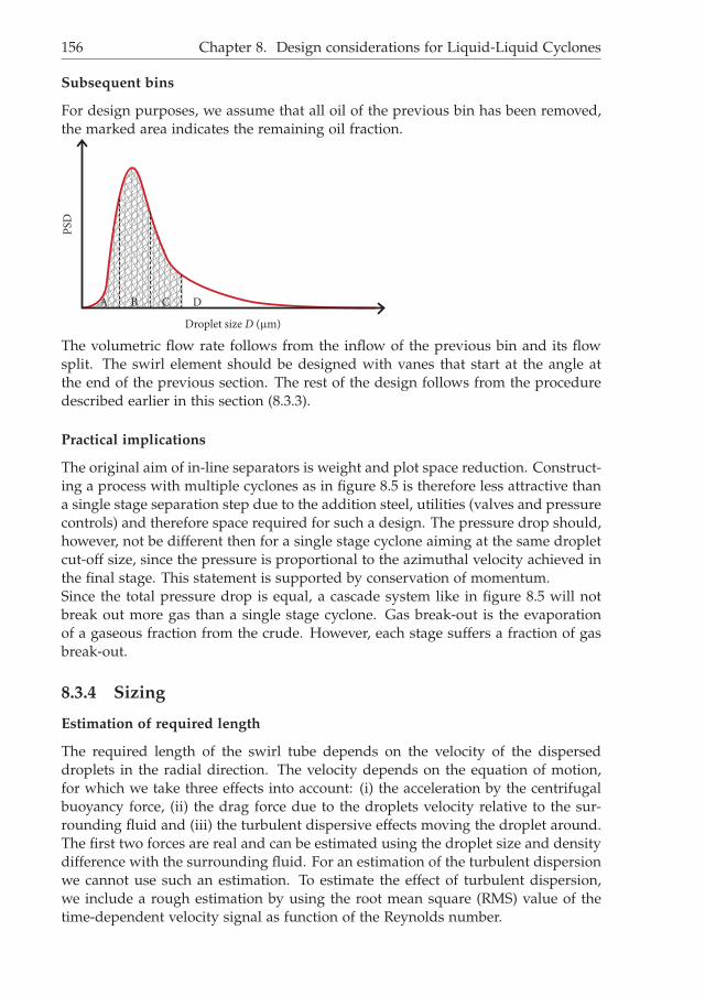
i

i

“Thesis1” — 2014/1/7 — 18:22 — page 156 — #176i

i

i

i

i

i


Subsequent bins

For design purposes, we assume that all oil of the previous bin has been removed,the marked area indicates the remaining oil fraction.

A B C D

Droplet size D (µm)

PSD

The volumetric flow rate follows from the inflow of the previous bin and its flowsplit. The swirl element should be designed with vanes that start at the angle atthe end of the previous section. The rest of the design follows from the proceduredescribed earlier in this section (8.3.3).

Practical implications

The original aim of in-line separators is weight and plot space reduction. Construct-ing a process with multiple cyclones as in figure 8.5 is therefore less attractive thana single stage separation step due to the addition steel, utilities (valves and pressurecontrols) and therefore space required for such a design. The pressure drop should,however, not be different then for a single stage cyclone aiming at the same dropletcut-off size, since the pressure is proportional to the azimuthal velocity achieved inthe final stage. This statement is supported by conservation of momentum.Since the total pressure drop is equal, a cascade system like in figure 8.5 will notbreak out more gas than a single stage cyclone. Gas break-out is the evaporationof a gaseous fraction from the crude. However, each stage suffers a fraction of gasbreak-out.

8.3.4 Sizing

Estimation of required length

The required length of the swirl tube depends on the velocity of the disperseddroplets in the radial direction. The velocity depends on the equation of motion,for which we take three effects into account: (i) the acceleration by the centrifugalbuoyancy force, (ii) the drag force due to the droplets velocity relative to the sur-rounding fluid and (iii) the turbulent dispersive effects moving the droplet around.The first two forces are real and can be estimated using the droplet size and densitydifference with the surrounding fluid. For an estimation of the turbulent dispersionwe cannot use such an estimation. To estimate the effect of turbulent dispersion,we include a rough estimation by using the root mean square (RMS) value of thetime-dependent velocity signal as function of the Reynolds number.

i

i

“Thesis1” — 2014/1/7 — 18:22 — page 157 — #177i

i

i

i

i

i


0 2 4 6 8 10 12

x 105

0

0.1

0.2

0.3

0.4

0.5

0.6

Reynolds number (Reθ)

RM

Sve

loci

ty(u

rms)

[m/s]

initial

weaker

larger

y = 4.83 10-7

x - 0.0068

Figure 8.6: RMS velocity as function of the Reynolds number based on the azimuthal velocity.

The method to approximate the required length of the cyclone does not considerall relevant effects. Although we do not intend on providing a full explanationwhy the phase separation in a liquid-liquid cyclone lacks behind the expectanciesbased on an ‘easy’ theory like below, there is one neglected effect. Droplets movinginward to the oil kernel push away the water, where the importance of droplet-droplet interactions increases rapidly. This effect is known as hindered settling,as described by the Richardson & Zaki correlation [40]. Increasing the length of acyclone beyond a critical value works counter effective on separation (see section7.1.2). The problem of hindered settling can thus not be ‘resolved’ with addingmore length to a cyclone.Figure 8.6 contains the root mean square averages for all different conditions asdiscussed in chapter 4. Although the relation is not fully linear, there is a positivecorrelation between the Reynolds number and the RMS velocity. The linear fit ofthe results is:

urms = 4.4 · 10−7Reθ − 0.0068, (8.11)

with the velocity in m/s.During the derivation of the droplets equation of motion, we treat the turbulentdispersive effect as a headwind equal to the rms-velocity of the single phase flow.The equation of motion then reads:

π

6D3

d (ρc − ρd)u2

θ

rd=

π

8D2

dρcCD (vr + urms)2 , (8.12)

where vr is the droplet radial velocity, which is < 0 for an inward moving dropletand u the continuous phase velocity. This leads to an estimation for the dropletvelocity in the radial direction:

i

i

“Thesis1” — 2014/1/7 — 18:22 — page 158 — #178i

i

i

i

i

i


vr = −√

43

Ddu2θ (ρc − ρd)

rdρcCD+ urms. (8.13)

The average displacement of all droplets can not become negative, if turbulent dis-persion dominates, the droplets will be equally distributed over the complete crosssection of the tube. Therefore, the interpretation of equation 8.13 is that for thosecases no separation is to be expected.The suggested length of the swirltube follows from the required displacement of oildroplets inward towards the oil kernel. The average distance that the droplets needto travel is estimated to be 1/4 of the tube diameter (not all droplets are at the wall,the oil kernel in the center has a finite size). The minimum required residence timein the cyclone is therefore:

∆t =Dt

4vr(8.14)

From chapter 4 we learned that the maximum axial velocity in the cyclone is in theorder of 2 times the bulk velocity upstream of the swirl element. Therefore, theminimum required length is:

L =2Φ

πDtvr(8.15)

Swirl tube diameter

The effect of diameter of the swirltube has not been tested within this research. Theavailable data in literature on cyclone design are limited to gas-solid cyclones witha different inlet geometry.When deciding on the diameter of a cyclone, the following considerations shouldbe taken into account:

1. To separate the phases, droplets should move in the radial direction, increas-ing the diameter, increases the maximum radial distance droplet should moveand works therefore counteractive on separation.

2. Drag at the wall slows down the vortex and is characterized by a large ∂v/∂r.This high shear is capable of tearing the droplets apart. From this perspective,a larger diameter is favorable.

3. The diameter is coupled to the axial velocity. The flow rate per cyclone and itsdiameter dictate the average axial velocity, where the axial velocity and lengthdetermine the residence time in the cyclone.

4. The volume flow requiring treatment and the composition of the stream arenot equal over the entire lifetime of a production facility. The water cut in-creases over time, where the total volume typically decreases. “Turn down” isoperating a facility below design specification. Turn down in a cyclone affectsthe azimuthal velocity and therewith the separation characteristic. For pro-cess design, it is therefore highly recommended to install multiple cyclones

i

i

“Thesis1” — 2014/1/7 — 18:22 — page 159 — #179i

i

i

i

i

i

8.4. Concluding remarks 159

in parallel to be able to run each cyclone at its optimal flow rate for givenseparation requirements.

The size of the swirl tube used in this research, being 10 cm, seems to be a reason-able compromise for points 1 to 3. Further research should be done to determinethe optimal diameter. The application of a gradual reduction of the tube diameterin the streamwise direction (tapering) can be beneficial, since it compensates for theloss of vortex strength due to friction. It is suggested to design the tapering suchthat the azimuthal velocity in the tube is kept as constant over length as possible,to avoid droplet breakup due to sudden regions with high shear.The total available cross section in the cyclones should be equal to, or larger thanthe cross section of the tube with the feed. A reduction in the cross section leadsto an acceleration of the fluid and those shear forces will break droplets, workingcounteractive on separation.

8.3.5 Process control

During operation of a cyclone, the pressure difference between the HPO and LPO ofeach cyclone(stage) determines the flow split (F = φLPO/φtot). From an operationalperspective, the flow split needs to be controlled, which can be done by the applic-ation of valves in one or both outlets. All valves used for pressure regulation exerta shear force on the liquids. This shear can break droplets and therefore hamperdownstream separation. Therefore, it is suggested to mount only a regulation valvein one outlet, the one which requires least downstream treatment.

8.3.6 Swirl element design

Within the ISPT project OG-00-004, a swirl element has been designed. This workwas performed at Twente University by Slot [13]. The considerations for the swirlelement design are discussed in section 4.2. The optimal design of the vanes andinternal body was not the scope of this thesis.the work of for example Slot [13] canbe used as design guide for the internal swirl element.

8.4 Concluding remarks

The motivation of the work presented in this thesis is to increase understanding ofin-line axial liquid-liquid cyclones, to strive for an optimal design, ready for applic-ation in industrial installations. In the preceding chapters, different aspects of thecyclone in our experimental facility were investigated.

Chapter 4: Single phase water study of the velocity and turbulence levels. Fromthe LDA data, the correlation between the swirl element design and resulting velo-city profile is better understood. The time series at different conditions form inputfor the modelling of turbulent dispersion.

Chapter 5: The time series of the velocity obtained in chapter 4 was used to solve

i

i

“Thesis1” — 2014/1/7 — 18:22 — page 160 — #180i

i

i

i

i

i


a simplified equation of motion for droplets in swirling flow, which provides amethod to predict the chance of separation for a specific droplet size in axial cyc-lones at a low numerical cost.

Chapter 6: Measurements of droplet sizes upstream and downstream of the swirlelement and cyclone itself provided relations for droplet breakup and coalescence.The breakup of droplets in a cyclone is the most important counteracting effect onseparation. From results in this chapter, a relation for the droplet sizes in the cyc-lone is obtained.

Chapter 7: The design was modified in many different ways to study the sensit-ivity of the separation efficiency to these changes. All changes that affected thedroplet size, such as flow rate and vane angle, proofed to be of major influence onthe separation quality, where the exact sizing such as the pickup tube diameter andlength did not affect separation much.

This chapter: Experimental data from chapters 6 and 7 is non-dimensionalized toobtain general conclusions on the expected separation efficiency for a broad rangeof cases. This leads to an aid for future design of liquid-liquid axial cyclones.

The conclusions of this thesis are not “ready to use” for companies that want toconstruct a device immediately applicable for field use. Although both experimentsand data evaluation were performed in a very careful manner, it is highly recom-mended to test the final conclusions. One can think of the construction of a multi-stage cyclone and the use of different liquids, to see whether the non-dimensionalresults work also for the other interfacial tension and density.

i

i

“Thesis1” — 2014/1/7 — 18:22 — page 161 — #181i

i

i

i

i

i

Bibliography

[1] D. Yergin. The Prize: The Epic Quest for Oil, Money & Power. Free Press, 2008.

[2] E. Bretney. Water-purifier. US Patent 453105, May 26 1891.

[3] M. Dirkzwager. A New Axial Cyclone Design for Fluid-Fluid Separation. PhDthesis, TU Delft, December 1996.

[4] D.A. Colman, M.T. Thew, and D.R. Corney. Hydrocyclones for oil/water sep-aration. In Proceedings of the 1st International Conference on on Hydrocyclones,Cambridge UK, pages 143–165, 1980.

[5] Y.J. Lu, L.X. Zhou, and X. Shen. Numerical simulation of strongly swirling tur-bulent flows in a liquid-liquid hydrocyclone using the Reynolds stress trans-port equation model. Science in China Series E-Technological Sciences, 43(1):86–96,2000.

[6] E.E. Paladino, G.C. Nunes, and L. Schwenk. CFD analysis of the transientflow in a low-oil concentration hydrocyclone. In Proceedings of the AIChE 2005Annual Meeting. AIChE, October 30 - November 4 2005.

[7] Sooran Noroozi and Seyed Hassan Hashemabadi. CFD Simulation of InletDesign Effect on Deoiling Hydrocyclone Separation Efficiency. Chemical Engin-eering & Technology, 32(12):1885–1893, 2009.

[8] Steffen Schütz, Gabriele Gorbach, and Manfred Piesche. Modeling fluid beha-vior and droplet interactions during liquid-liquid separation in hydrocyclones.Chemical Engineering Science, 64(18):3935–3952, 2009.

[9] Sina Amini, Dariush Mowla, and Mahdi Golkar. Developing a new approachfor evaluating a de-oiling hydrocyclone efficiency. Desalination, 285:131–137,2012.

[10] G.A.B. Young, W.D. Wakley, D.L. Taggart, S.L. Andrews, and J.R. Worrell. Oil-water separation using hydrocyclones - an experimental search for optimumdimensions. Journal of Petroleum Science and Engineering, 11(1):37–50, 1994.

[11] C. Oropeza-Vazquez, E. Afanador, L. Gomez, S. Wang, R. Mohan, O. Shoham,and G. Kouba. Oil-water separation in a novel liquid-liquid cylindrical cyclone(LLCC (c)) compact separator - Experiments and modeling. Journal of Fluids

161

i

i

“Thesis1” — 2014/1/7 — 18:22 — page 162 — #182i

i

i

i

i

i

162 Bibliography

Engineering-Transactions of the ASME, 126(4):553–564, 2004. 8th InternationalSymposium on Gas-Liquid Two-Phase Flows, Honolulu, HI, JUL 06-10, 2003.

[12] Trygve Husveg, Odile Rambeau, Tormod Drengstig, and Torleiv Bilstad. Per-formance of a deoiling hydrocyclone during variable flow rates. Minerals Engin-eering, 20(4):368–379, 2007. Hydrocyclones 2006 Conference, Falmouth, ENG-LAND, 2006.

[13] J.J. Slot. Development of a Centrifugal In-Line Separator for Oil-Water Flows. PhDthesis, Twente University, 2013.

[14] T. Krebs, K. Schroën, and R. Boom. Coalescence dynamics of surfactant-stabilized emulsions studied with microfluidics. Soft Matter, (8):10650–10657,2012.

[15] P.A. Yazdabadi, A.J. Griffiths, and N. Syred. Characterization of the PVC Phe-nomena in the Exhaust of a Cyclone Dust Separator. Experiments in Fluids, 17(1-2):84–95, June 1994.

[16] S. Leibovich. The Structure of Vortex Breakdown. Annual Review of Fluid Mech-anics, 10:221–246, 1978.

[17] O. Kito. Axi-Asymmetric Character of Turbulent Swirling Flow in a StraightCircular Tube. Bulletin of the JSME-Japan Society of Mechanical Engineers, 27(226):683–690, 1984.

[18] F. Durst, A. Melling, and J. H. Whitelaw. Principles and Practice of Laser-DopplerAnemometry. Academic Press Inc., 1976.

[19] M.J. Tummers. Investigation of a turbulent wake in an adverse pressure gradientusing Laser Doppler Anemometry. PhD thesis, Delft University of Technology,1999.

[20] R.J. Belt. On the liquid film in inclined annular flow. PhD thesis, Delft Universityof Technology, 2007.

[21] R.J. Adrian. Fluid mechanics measurements edited by R.J. Goldstein. Springer Ber-lin, 1983. Chapter V: Laser Velocimetry.

[22] J.H. Bae and L.L. Tavlarides. Laser Capillary Spectrophotometry for Drop-SizeConcentration Measurements. AiChE Journal, 35(7), 1989.

[23] S. Maaß , S Wollny, A. Voigt, and M. Kraume. Experimental comparison ofmeasurement techniques for drop size distributions in liquid/liquid disper-sions. Experiments in Fluids, 50(2), 2010.

[24] C. Desnoyer, O. Masbernat, and C. Gourdon. Experimental study of drop sizedistributions at high phase ratio in liquid-liquid systems. Chemical EngineeringScience, 58:1353–1363, 2002.

[25] James P.M. Syvitsky, editor. Principles, methods and application of particle sizeanalysis. Cambridge University Press, 1991.

i

i

“Thesis1” — 2014/1/7 — 18:22 — page 163 — #183i

i

i

i

i

i

Bibliography 163

[26] Paul A. Gunning, Martin S.R. Hennock, Andrew M. Howe, Alan R. Mackie,Peter Richmond, and Margaret M. Robins. Stability of oil-in-water emulsions.the effect of dispersed phase and polysaccharide on creaming. Colloids andSurfaces, 20(1-2):65 – 80, 1986.

[27] David J. Hibberd, Andrew M. Howe, and Margaret M. Robins. Use of concen-tration profiles in creaming emulsions to determine phase coexistence. Colloidsand Surfaces, 31(0):347 – 353, 1988. Proceedings of an International Conference.

[28] G.E. Mapstone. The Salting-out of Polyethylene Glycol Emulsifiers. Journal ofthe society of cosmetic chemists, pages 239 – 243, 1961.

[29] W. Harteveld. Bubble Columns: structures or stability? PhD thesis, Delft Univer-sity of Technology, 2005.

[30] H.-M. Prasser, A. Böttger, and J. Zschau. A new electrode-mesh tomograph forgas-liquid flows. Flow Measurement and Instrumentation, 9:111–119, 1996.

[31] D. Ito, H.-M. Prasser, H. Kikura, and M. Aritomi. Uncertainty and intrusive-ness of three-layer wire-mesh sensor. Flow Measurement and Instrumentation, 22:249–256, 2011.

[32] M.J. Da Silva and U. Hampel. Kapazitäts-Gittersensor: Prinzip und An-wendung. Technisches Messen, 77(4):209–214, 2010.

[33] P.M.T. Smeets. Master’s thesis, Delft University of Technology, Faculty of Ap-plied Sciences, Department of Multi-Scale Physics, 2007.

[34] D.J. Griffiths. Introduction to Electrodynamics. Prentice-Hall International, 1999.

[35] C.H.K. Williamson and G.L. Brown. A series in 1/√

re to represent the StrouhalReynolds number relationship of the cylinder wake. Journal of Fluids and Struc-tures, 12(8):1073 – 1085, 1998.

[36] Nikolay Ivanov Kolev. Multiphase Flow Dynamics 2, thermal and mechanical inter-actions. Springer-Verlag Berlin Heidelberg, 2007. ISBN 978-3-540-69834-0.

[37] J.O. Hinze. Fundamentals of the Hydrodynamic Mechanism of Splitting in Dis-persion Processes. American Institute of Chemical Engineering Journal, September1955.

[38] S. Galinat, O. Masbernat, P Guiraud, C Dalmazzone, and Noïk. Drop break-up in turbulent pope flow downstream of a restriction. Chemical EngineeringScience, 60:6511–6528, 2005.

[39] C.T. Crowe, J.D. Schwarzkopf, M. Sommerfeld, and Y. Tsuji. Multiphase Flowswith Droplets and Particles, second edition. CRC Press, Taylor & Francis Group,2012.

[40] Mamoru Ishii and Novak Zuber. Drag Coefficient and Relative Velocity inBubbly, Droplet or Particulate Flows. AIChE Journal, 25(5):843–855, 1979.

[41] I.H. Abbott. Theory of wing sections. McGraw-Hill, 1949.

i

i

“Thesis1” — 2014/1/7 — 18:22 — page 164 — #184i

i

i

i

i

i

164 Bibliography

[42] S. V. Alekseenko, P. A. Kuibin, V. L. Okulov, and S. I. Shtork. Helical vorticesin swirl flow. Journal of Fluid Mechanics, 382:195–243, 1999.

[43] Piet M. T. Broersen. The Removal of Spurious Spectral Peaks From Autore-gressive Models for Irregularly Sampled Data. IEEE Transactions on instrument-ation and measurement, 59(1):205–214, January 2010.

[44] H.E.A. van den Akker and R.F. Mudde. Fysische Transportverschijnselen I. VSSD,2003.

[45] Jaber Almedeij. Drag coefficient of flow around a sphere: Matching asymptot-ically the wide trend. Powder Technology, 186(3):218–223, 2008.

[46] P.G. Saffman. The lift on a small sphere in a slow shear flow. Journal of FluidMechanics, 22:385–400, 1965.

[47] H. Brauer. Umströmung beschleunigter und verzögerter Partikeln. Wärme- undStoffübertragung, 27:321–329, 1992.

[48] Yixiang Liao and Dirk Lucas. A literature review of theoretical models for dropand bubble breakup in turbulent dispersions. Chemical Engineering Science, 64:3389–3406, 2009. section 4.

[49] C. Martínes-Bazán, J.L. Montañés, and J.C. Lasheras. On the breakup of an airbubble injected into a fully developed turbulent flow. Part 2. Size PDF of theresulting daughter bubbles. Journal of Fluid Mechanics, 401:183–207.

[50] C.D. Eastwood, L. Armi, and J.C. Lasheras. The breakup of immiscible fluidsin turbulent flows. Journal of Fluid Mechanics, 502:309–333, 2004.

[51] G.K. Batchelor. Axial flow in trailing line vortices. Journal of Fluid Mechanics,20:645–658, 1964.

[52] Alan Reynolds. On the dynamics of turbulent vortical flow. Zeitschrift fürangewandte Mathematik und Physik ZAMP, 12:149–158, 1961. ISSN 0044-2275.

[53] O. Kitoh. Experimental study of turbulent swirling flow in a straight pipe.Journal of Fluid Mechanics, 225:445–479, April 1991.

[54] T. O’Doherty, A. J. Griffiths, N. Syred, P. J. Bowen, and W. Fick. Experimentalanalysis of rotating instabilities in swirling and cyclonic flows. Developments inChemical Engineering and Mineral Processing, 7(3-4):245–267, 1999.

[55] H. Tennekes and J.L. Lumley. A first course in turbulence. The MIT Press, 1972.

i

i

“Thesis1” — 2014/1/7 — 18:22 — page 165 — #185i

i

i

i

i

i

APPENDIX A

Description of swirling flow

This appendix provides a theoretical basis to describe swirling flow. The presentedtheory is based on single phase flow. The Navier-Stokes equations are given in thefirst section. Then, we provide an empirical description of swirling flow, i.e. theswirl number. The final section discusses vortex breakdown and characterization ofunsteady flow effects.

A.1 Governing equations

Conservation of momentum leads to the general description for fluid motion, theNavier-Stokes equations:

ρ

(∂~v

∂t+~v · ∇~v

)= −∇p + ∇ · ~T + ~f (A.1)

here ~T is the viscous stress tensor and ~f are body forces.Equation A.1 cannot be solved analytically. Assumptions or simplifications need tobe made to solve the equation:

• incompressible flow; the swirling flow deals only with liquids

• constant viscosity µ; the liquids used are all Newtonian at almost constanttemperature

• conservation of mass, given by the continuity equation: ∂ρ∂t + ~∇ · (ρ~v) = 0.

simplifies the Navier-Stokes equation to:

ρ

(∂~v

∂t+~v · ∇~v

)= −∇p + µ∇2

~v + ~f (A.2)

For cylindrical coordinates, this works out to the general case:

165

i

i

“Thesis1” — 2014/1/7 — 18:22 — page 166 — #186i

i

i

i

i

i

166 Appendix A. Description of swirling flow

ρ : ∂uz∂z + 1

r∂rur∂r + 1

r∂uφ

∂φ = 0 (A.3)

r : ρ

(∂ur∂t + ur

∂ur∂r +

uφ

r∂ur∂φ + uz

∂ur∂z − u2

φ

r

)=

− ∂p∂r + µ

(1r

∂∂r

(r ∂ur

∂r

)+ 1

r2∂2ur∂φ2 + ∂2ur

∂z2 − urr2 − 2

r2∂uφ

∂φ

)+ ρgr (A.4)

φ : ρ(

∂uφ

∂t + ur∂uφ

∂r +uφ

r∂uφ

∂φ + uz∂uφ

∂z +uruφ

r

)=

− 1r

∂p∂φ + µ

(1r

∂∂r

(r

∂uφ

∂r

)+ 1

r2∂2uφ

∂φ2 +∂2uφ

∂z2 + 2r2

∂ur∂φ − uφ

r2

)+ ρgφ (A.5)

z : ρ(

∂uz∂t + ur

∂uz∂r +

uφ

r∂uz∂φ + uz

∂uz∂z

)=

− ∂p∂z + µ

(1r

∂∂r

(r ∂uz

∂r

)+ 1

r2∂2uz∂φ2 + ∂2uz

∂z2

)+ ρgz (A.6)

So far, no analytical solution has been found that solves the set of equations above.Computational calculations taking into account the full Navier-Stokes equations areknown as Direct Navier-Stokes (DNS). For large systems, like the axial cyclone inthis thesis, the large range of sizes (µm to m and µs to s), DNS requires morecomputational power than a university has available.

A.2 Empirical description of swirling flow

The following assumptions improve understanding of equations A.4-A.6:

• Reynolds-Averaged Navier-Stokes: time-averaged decomposition of the ve-locity in a mean part and a time-dependent part: ui(t) = Ui + u′

i(t)

• Steady-state: ∂ui/∂t = 0 and ∂p/∂t = 0

• Axi-symmetry: ∂/∂φ = 0

• No net radial flow: Ur = 0.

With these assumptions, the Navier-Stokes equations work out to:

ρ : ∂Uz∂z + ∂u′

z∂z + 1

r∂ru′

r∂r = 0 (A.7)

r : ρ

(∂u′

ru′z

∂z − 1r

∂ru′2r

∂rU2

Φr +

u′2φ

r

)= ∂P

∂r (A.8)

φ : ρ

(Uz

∂Uφ

∂z + UrUφ

∂r +UrUφ

r +∂u′

φu′z

∂z + 1r

∂ru′ru′

φ

∂r +u′

ru′φ

r

)=

µ

(∂2Uφ

∂z2 + 1r

∂∂r

(r

∂Uφ

∂r

)− Uφ

r2

)(A.9)

z : ρ

(Uz

∂Uz∂z + ∂u

′2z

∂z − 1r

∂ru′ru′

z∂r

)= µ

(∂2Uz∂z2 + 1

r∂∂r

(r ∂Uz

∂r

))− ∂P

∂z (A.10)

i

i

“Thesis1” — 2014/1/7 — 18:22 — page 167 — #187i

i

i

i

i

i

A.3. Swirl number 167

For the condition ∂/∂z ≪ ∂/∂r Batchelor [51] found an analytical solution:

Ur(r) = 0 (A.11)

Uφ(r) = qW0r0

r

(1 − e

−(

rr0

)2)

(A.12)

Uz(r) = U∞ − W0e−

(r

r0

)2

(A.13)

with q the balance between axial and azimuthal velocity, W0 the axial vortex velocity,r0 the characteristic vortex radius and U∞ the maximum axial velocity (found at theupstream side). This approximation of the flow holds when viscous transport ofmomentum is dominant, which holds only for laminar flow. Reynolds [52] providesa more accurate derivation from a physics perspective. Results with the model ofBatchelor [51], however, have a reasonable agreement with experimental data (seefor example Dirkzwager [3]) and is practical in use. Even with current computingpower and physical modelling, Slot [13] shows it is hard to provide an accuratemodel of the flow.

A.3 Swirl number

The swirl intensity in pipe flow can be expressed in terms of a non-dimensionalnumber, this is the Swirl number Ω. There are various definitions for the swirlnumber [3] , we use the formulation as provided by Kitoh [53]:

Ω =2πρc

∫ R0 uzuθr′2dr′

ρcπR3u2b

(A.14)

with ρc the liquid density, uz the axial velocity, uθ the azimuthal velocity, R the tuberadius and ub the liquid bulk velocity.The interpretation of Ω is not straightforward. The integral in the numerator in-volves two parameters: (i) the angular momentum of a finite volume (~r × ~p =ρruθdV) and (ii) the distribution of the mass flux over the radius (ruz). These quant-ities are non-dimensionalized in the nominator with the mass flux (ρπR2ub) andthe term Rub.

Due to friction at the wall, the swirl intensity Ω decreases in the downstream dir-ection. The relation between the swirl intensity at distance z has been estimated byDirkzwager [3]:

Ω(z) = Ω0e−Cdz−zr

D , (A.15)

with Ω0 the swirl number at position zr where it is generated and Cd a decaycoefficient.

i

i

“Thesis1” — 2014/1/7 — 18:22 — page 168 — #188i

i

i

i

i

i

168 Appendix A. Description of swirling flow

A.4 Advanced concepts

The preceding section provided us with empirical relations to understand the basicsof swirling flow. The simplifications in the parametrization do not allow to accountfor time-dependent effects

A.4.1 Vortex Breakdown and flow reversal

A vortex is a fluid structure performing a helical motion, where both the axial andazimuthal velocity are over the complete cross section in the same direction. Vortexbreakdown is the phenomenon that the vortex does not stretch across the completetube diameter, but leaves a region around the centreline that has a velocity in theopposite direction. This looks like a helical flow around a virtual body, a bodybeing fluid flow in the reversed direction.The vortex breakdown in the axial cyclone is apparent as a region with reverse flow.Although the complete description of the flow would require the analytical solutionof the Navier-Stokes equations (eq. A.4 to A.6, the driving force can be understoodwith a simpler concept. Consider four points in the tube: (i) close to the swirlelement near the wall, (ii) far downstream, just before the end of the tube with theswirling flow, close to the wall, (iii) far downstream, just before the end of the tubewith the swirling flow, in the center and (iv) close to the swirl element in the center.The pressure difference between the points at the same axial position (e.g. (i) vs.(iv) and (ii) vs. (iii)) are given by:

∆p =∫ r2

r1

ρv2θ

rdr. (A.16)

Due to the decrease in swirl strength in the axial direction, ∆p decreases for increas-ing axial distance to the swirl element. Therefore, the relation between the differentpressures is as follows: p(i) > p(ii) > p(iii) > p(iv). The pressure gradient on thecenterline is opposite to the bulk flow direction, resulting in a reverse flow region.According to O’Doherty et al. [54] recirculation zones are formed for flows with aswirl number above 0.6.

A.4.2 Time-independent instabilities

The equations describing cyclonic fluid flow (eq. A.4-A.6) do not contain forces thatcan break symmetry from itself. Without any external disturbance, axi-symmetricalflow remains axi-symmetrical, almost all terms in A.4 are zero or counterbalancing.There are many sources that can contribute to a non-symmetric radial velocity: (i)non-symmetric inflow of liquid, caused by bends, (ii) lack of symmetry in the swirlgenerating device, (iii) lack of symmetry in the tube surrounding the vortex or (iv)non-orthogonal placement of the cyclone with respect to earths gravity.Equations A.8 - A.10 show that these effects also hold for the time-averaged case,which leads to a vortex spiralling around a helical core.The vortex breakdown includes also the introduction of asymmetry - what does this

i

i

“Thesis1” — 2014/1/7 — 18:22 — page 169 — #189i

i

i

i

i

i

A.4. Advanced concepts 169

do for the flow. O’Doherty et al. [54] report axial-symmetric vortex-flow only existsfor very low Re and Ω: Re < 1000 and Ω < 0.6.

i

i

“Thesis1” — 2014/1/7 — 18:22 — page 170 — #190i

i

i

i

i

i

170

i

i

“Thesis1” — 2014/1/7 — 18:22 — page 171 — #191i

i

i

i

i

i

APPENDIX B

Estimation of turbulence parameters

Idea of this paragraph: (i) the system we look at is turbulent, (ii) the consequence ofturbulence is the existence of turbulent eddies (iii) these eddies transfer momentumto other directions and to other scales (iv) dispersed droplets are sensitive to thismomentum transfer.

B.1 Turbulence

The effect of turbulence of the flow is the existence of eddies at different sizes,ranging from the Kolmogorov microscale to the size scale of the flow (in our case:the diameter of the tube). The turbulent eddies are important, since they will ex-ert a force on dispersed droplets. For droplets below a critical diameter Dcrit theimpulse by the turbulent eddies drag exceeds the momentum of the droplets - thedispersed droplets will act like flow tracers. On the bulk scale, this effect is knownas turbulence dispersion.

Smallest length scale To quantify the effect of turbulent eddies in our swirlingflow, the time-dependent velocity data obtained with LDA is used. Due to theirregular interarrival times of the tracer particles, a frequency analysis which rangesbeyond the average sampling rate can be done. The average sampling frequencywas 10 to 1000 Hz.The irregular LDA data was examined with the ARMAsel (Auto Regressive Methodfor Spectral Analysis) as provided by Broersen [43]. It is very unlikely that the tur-bulence in our system is isotropic. It is however feasible to guess that the radial andaxial direction contain the same amount of turbulence. We only have measurementdata for the axial and azimuthal velocity. Figure B.1 shows a characteristic turbu-lent spectrum, where the frequency drops for frequencies beyond the integral timescale. The smallest scales are on the right size of this spectrum.We conducted a procedure to estimate the scale of the smallest eddies in the flowbased on the procedure described by Tennekes and Lumley [55]. The relevantquantities are (i), the turbulent dissipation rate:

171

i

i

“Thesis1” — 2014/1/7 — 18:22 — page 172 — #192i

i

i

i

i

i

172 Appendix B. Estimation of turbulence parameters

100

101

102

103

104

10−6

10−5

10−4

10−3

10−2

→ frequency [Hz]

→ L

ogar

ithm

of p

ower

spe

ctra

l den

sity

Figure B.1: Example of a time spectrum estimate with Armasel. Data for the strong swirlelement, 56 m3/h, r = 12.5 mm, azimuthal velocity at 782 mm downstream.

ǫ = 2νsijsij = 15ν

(∂u1

∂x1

)2

, (B.1)

and (ii) the Kolmogorov microscale:

η =

(ν3

ǫ

)1/4

. (B.2)

For each point of interest, the estimate of the turbulent time spectrum was calcu-lated with ARMAsel like in figure B.1. According to Tennekes and Lumley [55] theintegral scale is given by ωℓ

u = 2.4 This is the point where the curve starts to bend.From that, we derive ℓ

u . The end of this graph is marked by the position ωηv = 0.74

with ω the frequency, η the Kolmogorov length scale and v the Kolmogorov velocityscale. From this value the turbulent dissipation rate η is calculated and therewiththe Kolmogorov length η.

B.2 Method

According to Tennekes and Lumley [55] (page 279), the integral scale is given byωℓu = 2.4; this is the point where the curve starts to bend from horizontal to the

i

i

“Thesis1” — 2014/1/7 — 18:22 — page 173 — #193i

i

i

i

i

i

B.3. Result 173

descending slope. Based on this condition, for each velocity component (both azi-muthal and axial), the value of ℓ

u can be approximated. From Tennekes and Lumley[55] it follows that the end of the frequency graph, where the power spectrum in-creases more rapidly, is marked by the position ωη

v = 0.74 with ω the frequency, ηthe Kolmogorov length scale and v the Kolmogorov velocity scale. From the valuefor ω at the end of the curve, the turbulent dissipation rate η is calculated andtherewith the Kolmogorov length η.The procedure above is performed for the selected flow rate and measurement po-sition, a part of 1000 time steps from each time series was obtained.

B.3 Result

The method mentioned above has been applied on a dataset of the strong andweak swirl element at a flow rate of 56 m3/h. Figure B.2 shows the estimatesfor the smallest scales at different radial positions and for the different velocitycomponents.The smallest eddies are found at r = 40 mm. Figure 4.6 shows the velocity profilesfor the different swirl elements. The azimuthal velocity profile is rather flat at r = 40mm, but the axial velocity has almost its maximum velocity over there. The hightotal velocity leads to high turbulence production and therewith small eddies.

Accuracy The results shown in figure B.2 should have a large uncertainty. Al-though the method makes it hard to quantify this, the laborious process to cometo the results in combination with the required subjective data evaluation makesresults not highly reproducible, as can be seen for the weak swirl element at r = 20mm.The method in chapter 5 proofed to be a more stable predictor of turbulent disper-sion, than the estimate of the Kolmogorov scale provided in this appendix.

i

i

“Thesis1” — 2014/1/7 — 18:22 — page 174 — #194i

i

i

i

i

i

0 5 10 15 20 25 30 35 40 45 500

5

10

15

20

25

30

35

40


Kol

mogo

rov

lengt

h(η

)[µ

m]

Strong, Azimuthal

Strong, Axial

Weak, Azimuthal

Weak, Axial

Figure B.2: Estimate for the Kolmogorov length scale based on the axial and azimuthalvelocities. Flow rate: 56 m3/h, flow split = 0.3 and measurement 782 mm downstream of thestrong swirl element

174

i

i

“Thesis1” — 2014/1/7 — 18:22 — page 175 — #195i

i

i

i

i

i

APPENDIX C

Uncertainty analysis

The rig is equipped with fixed measurement devices for the flow rates, pressures,density and interface levels. Besides these devices, there is temporary measurementequipment, such as the Laser Doppler apparatus, the wire-mesh, endoscope, opticalprobes etc. This section deals with the measurement results of the fixed equipment.

C.1 Accuracy of the measurement equipment

Float flow meters The inflow of oil and brine is measured with float flow meterstype Heinrichs BGN with a specified measurement error of 1.28 m3/h.

Coriolis flow meter The flow in the HPO is measured with a Coriolis flow meterof Emerson type MicroMotion Elite CMF300. The error in the mass flow is 0.10 %,for the density 0.5 kg/m3.

Oil cut in the HPO The oil cut in the HPO is derived according to the followingequation:

cHPO =ρHPO − ρbrine

ρoil − ρbrine. (C.1)

Temperature dependence The densities of oil and brine (in kg/m3) are calculatedbased on temperature T(in C), according to the following relations:

ρbrine(T) = −0.5202[

kgCm3

]T [C] + 1074.7 [kg/m3], (C.2)

ρoil(T) = −0.7417[

kgCm3

]T [C] + 891.41 [kg/m3], (C.3)

these relations are experimentally determined with the density measurements inthe Coriolis flow meter present in the rig.

175

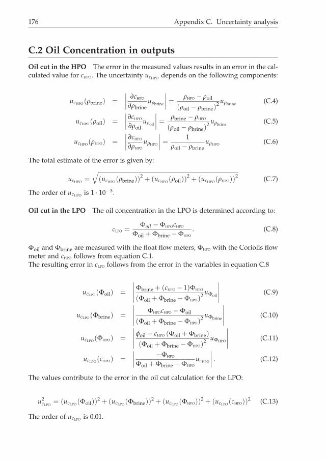
i

i

“Thesis1” — 2014/1/7 — 18:22 — page 176 — #196i

i

i

i

i

i

176 Appendix C. Uncertainty analysis

C.2 Oil Concentration in outputs

Oil cut in the HPO The error in the measured values results in an error in the cal-culated value for cHPO. The uncertainty ucHPO depends on the following components:

ucHPO(ρbrine) =

∣∣∣∣∂cHPO

∂ρbrineuρbrine

∣∣∣∣ =ρHPO − ρoil

(ρoil − ρbrine)2 uρbrine (C.4)

ucHPO(ρoil) =

∣∣∣∣∂cHPO

∂ρoiluρoil

∣∣∣∣ =ρbrine − ρHPO

(ρoil − ρbrine)2 uρbrine (C.5)

ucHPO(ρHPO) =

∣∣∣∣∂cHPO

∂ρHPO

uρHPO

∣∣∣∣ =1

ρoil − ρbrineuρHPO (C.6)

The total estimate of the error is given by:

ucHPO =

√(ucHPO(ρbrine))

2 + (ucHPO(ρoil))2 + (ucHPO(ρHPO))

2 (C.7)

The order of ucHPO is 1 · 10−3.

Oil cut in the LPO The oil concentration in the LPO is determined according to:

cLPO =Φoil − ΦHPOcHPO

Φoil + Φbrine − ΦHPO

. (C.8)

Φoil and Φbrine are measured with the float flow meters, ΦHPO with the Coriolis flowmeter and cHPO follows from equation C.1.The resulting error in cLPO follows from the error in the variables in equation C.8

ucLPO(Φoil) =

∣∣∣∣∣Φbrine + (cHPO − 1)ΦHPO

(Φoil + Φbrine − ΦHPO)2 uΦoil

∣∣∣∣∣ (C.9)

ucLPO(Φbrine) =

∣∣∣∣∣ΦHPOcHPO − Φoil

(Φoil + Φbrine − ΦHPO)2 uΦbrine

∣∣∣∣∣ (C.10)

ucLPO(ΦHPO) =

∣∣∣∣∣φoil − cHPO (Φoil + Φbrine)

(Φoil + Φbrine − ΦHPO)2 uΦHPO

∣∣∣∣∣ (C.11)

ucLPO(cHPO) =

∣∣∣∣−ΦHPO

Φoil + Φbrine − ΦHPO

ucHPO

∣∣∣∣ . (C.12)

The values contribute to the error in the oil cut calculation for the LPO:

u2cLPO

= (ucLPO(Φoil))2 + (ucLPO(Φbrine))

2 + (ucLPO(ΦHPO))2 + (ucLPO(cHPO))

2 (C.13)

The order of ucLPO is 0.01.

i

i

“Thesis1” — 2014/1/7 — 18:22 — page 177 — #197i

i

i

i

i

i

C.2. Oil Concentration in outputs 177

Coriolis flow meter in the LPO In the last months of the project, a Coriolis flowmeter was installed in the LPO. This flow meter was a Endress+Hauser Promass83I with a nominal diameter of 50mm. This flow meter has a specified error forthe mass flow of 0.10 % of the measured value and 0.5 kg/m3 for density. Thisbrings the measurement error for the volumetric oil concentration in the LPO to theorder of the error for the HPO: 10−3. The error is indicated in the graph with therespective results.

i

i

“Thesis1” — 2014/1/7 — 18:22 — page 178 — #198i

i

i

i

i

i

178

i

i

“Thesis1” — 2014/1/7 — 18:22 — page 179 — #199i

i

i

i

i

i

APPENDIX D

Drag relation for a sphere

In this work, we use the drag estimation for a sphere as provided by Almedeij [45]for all Reynolds numbers smaller than 106.The drag coefficient CD is given by:

CD =

[1

(φ1 + φ2)−1 + φ−1

3

+ φ4

]1/10

(D.1)

where the different functions φ are given by:

φ1 =(

24Re−1)10

+(

21Re−0.67)10

+(

4Re−0.33)10

+ (0.4)10

φ2 =1

(0.148Re0.11

)−10+ (0.5)−10

φ3 =(

1.57 · 108Re−1.625)10

φ4 =1

(6 · 10−17Re2.63

)−10+ (0.2)−10

.

Figure D.1 displays equation D.1.

179

i

i

“Thesis1” — 2014/1/7 — 18:22 — page 180 — #200i

i

i

i

i

i

100

101

102

103

104

105

106

10−2

10−1

100

101

102

Reynolds number (Re)

Dra

gco

effici

ent

(CD

)

Figure D.1: Drag coefficient as function of the Reynolds number for the relation in equationD.1.

180

i

i

“Thesis1” — 2014/1/7 — 18:22 — page 181 — #201i

i

i

i

i

i

List of publications

Papers

1. L.J.A.M. van Campen and R.F. Mudde, Droplet breakup in an Axial Cyclone,paper and oral presentation for the International Conference on MultiphaseFlow, Jeju (South Korea), May 2013.

2. L.J.A.M. van Campen, J.J. Slot, R.F. Mudde and H.W.M. Hoeijmakers, A numer-ical and experimental survey of a liquid-liquid axial cyclone, International Journalof Chemical Reaction Engineering, Volume 10, issue 1, June 2012.

3. L.J.A.M. van Campen, J.J. Slot, R.F. Mudde and H.W.M. Hoeijmakers, Anaxial cyclone for oil/water separation, conference paper for the 12th InternationalConference on Multiphase Flow in Industrial Plants, Ischia (Italy), September2011.

4. L.J.A.M. van Campen and R.F. Mudde, Direct droplet size measurements in anoil/water axial cyclone, to be submitted to the International Journal of Mul-tiphase Flow.

Patent

1. Eckhard Schleicher, Martin Löschau, Laurens van Campen, Gittersensor fürhochleitfähige Medien, patent submitted to the Munich Patent office.

181

i

i

“Thesis1” — 2014/1/7 — 18:22 — page 182 — #202i

i

i

i

i

i

182

i

i

“Thesis1” — 2014/1/7 — 18:22 — page 183 — #203i

i

i

i

i

i

Acknowledgements

Wetenschappelijk onderzoek is niet iets wat je als kluizenaar tot een goed eindekan brengen. De interactie met collega’s, stafleden, de industrie en de rest van debuitenwereld is essentieel: ik had niet zonder gekund. Deze drie pagina’s gevenmij de gelegenheid alle betrokkenen te benoemen die zeer hebben bijgedragen aande totstandkoming van dit proefschrift.

Allereerst ben ik Rob erkentelijk dat hij me in de zomer van 2008 benaderde omdit project te doen. Waar ik aanvankelijk het doen van een promotieonderzoek nietals serieus vervolg van mijn carrière beschouwde, had dit project de juiste mix vanwetenschap, industiële inmenging en experimenteel geknutsel om mij enthousiastte maken. De grote mate van verantwoordelijkheid die je aan me overliet, heeft mezeer gevormd en daar heb ik nog dagelijks profijt van.Harry Hoeijmakers bevond zich als tweede promotor hemelsbreed op grote afstand,maar was altijd beschikbaar om binnen en buiten de geplande ISPT progress mee-tings mee te denken. Ook Karin Schroën (WUR) had een belangrijke rol, niet alleenvanwege de fysisch-chemische inzichten, maar ook vanwege de nimmer aflatendebemoedigende opmerkingen en recordsnelheid van het beantwoorden van e-mails!Jesse en Thomas, als collega-onderzoekers in ons ISPT project bedank ik jullie zeervoor alle discussies die we hebben gehad. Juist de verschillen in onze achtergrondenmaakten dat we veel verschillende aspecten van onze olie water axiaal cycloon goedhebben kunnen bekijken.Het bijzondere van dit ISPT project was de grote interactie met “de industrie”. Ditproject had nooit bestaan zonder de drijvende kracht van Paul Verbeek, die in allefases van het project nauw betrokken was. Ook al heb ik Wouter Harteveld (Shell)slechts enkele keren gesproken, zijn bevlogenheid en ideeënrijkheid heeft me ergaangestoken. Frames heeft in de personen van Johanna en Martijn veel tijd en moei-te in het project gestoken, uiteenlopend van nadenken over het ontwerp van eennieuw swirlelement, tot de technische aanbesteding van een nieuw scheidingsvat,alles werd snel en precies opgevolgd. Danny van der Krogt van Wintershall heeftveel bijgedragen aan mijn inzicht van de dagelijkse praktijk van hydrocarbon recove-ry, zodat ik ons eigen werk beter in een breed perspectief kon plaatsen. Tenslottewil ik Arian Nijmeijer (squash!), Peter Veenstra en Remko Westra niet onbenoemdlaten.

183

i

i

“Thesis1” — 2014/1/7 — 18:22 — page 184 — #204i

i

i

i

i

i

184 Acknowledgements

Tijdens mijn werkzaamheden maakte ik deel uit van de afdeling Multi-Scale Phy-sics (tot 31-8-2012) en de sectie Transport Phenomena (vanaf 1-9-2012). Het meema-ken van de herijking die aan deze naamswijziging ten grondslag lag en de weerslagdie dat had op de (ondersteunende) staf, hebben op mij grote indruk gemaakt. Ikben blij dat de groep als geheel er in mijn ogen hechter uit is gekomen.Het bouwen van een grote experimentele opstelling zoals in dit onderzoek, is nietalleen mogelijk. Alle lof voor Jan en Jaap (K) die zo vlak voor hun pensioen nog ditfysiek zware werk zo netjes hebben uitgevoerd. Jaap (vR), Evert, Wouter, Lodi enThea, bedankt voor alle kleine en grote klussen waar jullie me bij hebben geholpen.Nog een speciaal woord van dank voor Jaap Kamminga die me alle essentiële vaar-digheden heeft bijgebracht om in het laatste jaar zonder technicus de opstelling zelfdraaiende te kunnen houden.Naast de ondersteuning in het lab, mag ik de secretariële ondersteuning niet ver-geten: Amanda, Angela, Anita en Fiona, dankjewel! Typically, the office mates arethose who you see most often (at least, when your lab is nearby). And whetherit was W220, 34B-3C-1-160 of 0.519, I’d like to thank Annekatrien, Özgür, Adrian,Zaki, Anton, Michiel, Bernhard, Duong and Wenjie for the pleasant moments to-gether, the patience with all my complaints and frustrations and last but not least,for keeping the pranks with my workspace within reasonable limits.In de loop van de tijd hebben vijf studenten met mij gewerkt aan een gerelateerdproject. Als eerste Wout aan een onderzoek om druppels te volgen met een hoge-snelheidscamera. Vervolgens kwam Yoerik als MSc student om het werk van Woutvoort te zetten (zowel experimenteel als numeriek). Bauke en Rik hebben gewerktaan hun BEP bij mij. Matty heeft veel werk verzet aan de geometrievariaties die jevindt in hoofdstuk 7.Ook met andere studenten en aio’s was het prettig optrekken, van de koffiepauzetot op de curlingbaan of de grotten in Limburg: Rudi, Rick, Alexander, Niels, Koen,Cees, Matthijs, Maarten, Aljen, Gijs en Rosanne: ’t was gezellig! En Dries, als ‘vaste’reisgenoot hebben we toch aardig wat gezien van de wereld (in ieder geval Italië,Zuid-Korea en Japan - alleen jammer van de karaoke... ;)Altough Luis Portela was not formally involved in the work of this thesis, it is greatto have an “encyclopedia on fluid dynamics” nearby. Where the converstationsdid not only turbulence and its measurements, but extended to the weal and woeof university life. Ook Stephanie Hessing heeft onbewust veel coaching verzorgdbinnen het thema how to manage your manager, bedankt!

De boog kan niet altijd gespannen staan: veel zaken die op ’t eerste gezicht nietsmet een olie/watercycloon te maken hebben, hebben zeker zowel afleiding als in-spiratie gegeven.In de loop van de tijd heb ik het genoegen gehad heel wat sportactiviteiten te mo-gen organiseren: de WinterWedstrijden (roeien), het Europees Universiteitskampi-oenschap roeien in 2010, de NSRF Slotwedstrijden van 2011 t/m 2013 en de wie-lerronde van Delft van 2011 t/m 2013. Het is mooi om te zien hoe je met een heeldiverse groep, grote dingen kan opzetten, plus, je leert jezelf goed kennen. Allebetrokkenen, het was mooi met jullie samen te werken!Als jury was ik bij menig roeiwedstrijd te vinden, op of aan het water. Naast

i

i

“Thesis1” — 2014/1/7 — 18:22 — page 185 — #205i

i

i

i

i

i

185

gezellige dagen is het leuk om je kennissenkring uit te breiden buiten de technischehoek, maar wel veilig met Ons Soort Mensen.Mens sana in corpore sano: op de fiets en op de schaats! Waar de technische uitdagingvan fietsen te vinden is in de nieuwste mechanische snufjes, is de schaatstechniekeen uitdaging waar ik mijn tanden nog tot in het vrijwel oneindige op stuk kanbijten. In ieder geval, WTOS’ers en ELSjes, bedankt voor de mooie tijd!

Zelf had ik nooit zo ver kunnen komen zonder de liefdevolle en kansenrijkeopvoeding van mijn ouders en ondersteuning die er tot op de dag van vandaag isals het nodig is. Ook mijn broer, zus, zwager, neefje en nichtje, het is altijd goed omte zien dat er meer in het leven is dan promoveren. En last but not least, Ingeborg,ook al heb je alleen het laatste stukje van het werk van dichtbij meegemaakt, ik benblij dat ik alle hoogte- en dieptepunten met jou heb kunnen delen!

Laurens van Campen

Delft, november 2013

i

i

“Thesis1” — 2014/1/7 — 18:22 — page 186 — #206i

i

i

i

i

i

186

i

i

“Thesis1” — 2014/1/7 — 18:22 — page 187 — #207i

i

i

i

i

i

Curriculum Vitae

I was born on the 25th of May, 1984 in Nijmegen, The Nether-lands. I grew up in Veghel, where I went to primary school,afterwards I joined Gymnasium Bernrode in Heeswijk as sec-ondary school. After graduation at the gymnasium in 2002, myeducation continued at Delft University of Technology with theBachelor and Master programme Applied Physics, completedin February 2009 at the Department Radiation, Radionuclides& Reactors Department. The title of my MSc thesis was “Anexperimental investigation on the use of FEP as refractive in-dex matching material for LDA in rod bundle flow”.

Following my MSc thesis work, I started in 2009 the PhD programme of whichthis thesis is the result, with prof. dr. Rob Mudde as thesis advisor, first in theDepartment of Multi-Scale Physics, from September 2012 onwards in the sectionTransport Phenomena of the Department of Chemical Engineering.I started October 7th, 2013 as Researcher Natural Gas Treating at Shell Global Solu-tions International in Amsterdam.

187

Bu

lk Dyn

amics of D

roplets in

Liqu

id-Liq

uid

Axial C

yclones Laurens van C

ampen

Bulk Dynamics of Droplets in Liquid-Liquid Axial Cyclones

Laurens van Campen9 789064 647369

ISBN 978-90-6464-736-9

Bulk Dynamics of Droplets in Liquid-Liquid Axial Cyclones

Documents