Boris Blagov. Financial Crises and Time-Varying Risk Premia in a Small Open Economy: A Markov-Switching DSGE Model for Estonia

Financial Crises and Time-Varying Risk Premia ina Small Open Economy: A Markov-Switching

DSGE Model for Estonia

Boris Blagov

University of Hamburg

September 2013

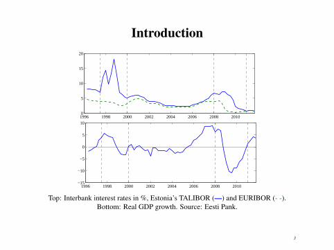
Introduction

• Non-linearities in DSGE models• Currency board in DSGE models

Absence of money

Fixed exchange rate

4e = 0

Identity between the interest rates (Galí 2008)

i = i∗

2

Introduction

1996 1998 2000 2002 2004 2006 2008 20100

5

10

15

20

1996 1998 2000 2002 2004 2006 2008 2010−15

−10

−5

0

5

10

Top: Interbank interest rates in %, Estonia’s TALIBOR (—) and EURIBOR (- -).Bottom: Real GDP growth. Source: Eesti Pank.

3

Model Overview

• Follows Benignio (2001), Monacelli (2005), Justiniano and Preston(2010)

• Consumers maximize utility by choosing consumption and labour,have access to foreign markets

• Consumption is a bundle of home produced goods (H) and importedgoods (F)

• Nominal rigidities in terms of sticky prices (hybrid inflationdynamics)

• Perfect labour market• LOOP does not hold/incomplete asset markets/imperfect risk sharing• Currency board (fixed exchange rate)• Markov-Switching component

4

The ModelDomestic Demand: Consumers maximize utility

E0

∞

∑t=0

βtϑt

[C1−σ

t

1−σ− N1+ϕ

t

1+ϕ

]s.t.

PtCt +Bt + etB∗t = Bt−1(1+ it−1)+ etB∗t−1(1+ i∗t−1)Φ(Dt)+WtNt +Tt

• Φ(Dt,φt) is a debt elastic interest rate premium with

Φt = exp−χ(Dt +φt)• Dt is the real quantity of the consumer’s net foreign asset position in

relation to steady state output Y

Dt =EtB∗t−1

YPt−1

• The usual Euler equation applies

5

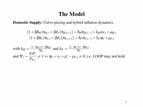
The ModelDomestic Supply: Calvo pricing and hybrid inflation dynamics

(1+βδH)πH,t = βEtπH,t+1+δHπH,t−1 +λHmct +µH,t

(1+βδF)πF,t = βEtπF,t+1+δFπF,t−1 +λFψt +µF,t

with λH = (1−θH)(1−βθH)θH

and λF = (1−θF)(1−βθF)θF

and Ψt =EP∗tPF,t

6= 1⇔ ψt = et +p∗t −pF,t 6= 0, i.e. LOOP may not hold

6

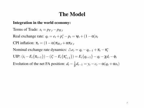
The ModelIntegration in the world economy:

Terms of Trade: st = pF,t−pH,t

Real exchange rate: qt = et +p∗t −pt = ψt +(1−α)st

CPI inflation: πt = (1−α)πH,t +απF,t

Nominal exchange rate dynamics: 4et = qt−qt−1 +πt−π∗t

UIP: (it−Etπt+1)− (i∗t −Etπ∗t+1) = Etqt+1−qt−χdt−φt

Evolution of the net FA position: dt− 1β

dt−1 = yt− ct−α(qt +αst)

7

The ModelMonetary policy:

4et = 0substituting through the above equations:

it = i∗t −χdt−φt

Exogenous Processes

φt = ρφφt−1 + εφ

t with εφ

t ∼ N(0,σ2φ(st))

at = ρaat−1 + εat with ε

at ∼ N(0,σ2

a)

ϑt = ρϑϑt−1 + εϑt with ε

ϑt ∼ N(0,σ2

ϑ)

µH,t = ρµµH,t−1 + εµHt with ε

µHt ∼ N(0,σ2

µH)

µF,t = ρµµF,t−1 + εµFt with ε

µFt ∼ N(0,σ2

µF)

y∗t = cy∗y∗t−1 + εy∗t with ε

y∗t ∼ N(0,σ2

y∗)

π∗t = cπ∗π

∗t−1 + ε

π∗t with ε

π∗t ∼ N(0,σ2

π∗)

i∗t = ci∗i∗t−1 + εi∗t with ε

i∗t ∼ N(0,σ2

i∗)

8

Markov-Switching extensionThe different states are characterized by time-varying stochastic volatilityof the risk-premium

φt = ρφφt−1 + εφ

t with εφ

t ∼ N(0,σ2φ(st))

which evolve according to

P =

[p11 p12p21 p22

]The equations may then be cast in the following matrix form:

B1(st)xt = EtA1(st,st+1)xt+1+B2(st)xt−1 +C1(st)zt

zt = R(st)zt−1 + εt with εt ∼ N(0,Σ2(st))

9

Solving a Markov-switching DSGE Model

• 2nd Order Perturbation Method (Foerster et.al [2013], wp)• Forward Solution Method (Cho [2011], wp)• Minimal State Variable (MSV) Solution method (Farmer et.al [2011],

JEDC)• Solution under bounded shocks (Davig and Leeper [2007], AER)

The first three use unbounded shocks and use the notion of a MSVsolution. That is, the system has a solution of the sort:

xt = Ωxt−1 +Γεt +ϒwt

with xt = ΩXt−1 +Γεt being the "fundamental part" and ϒwt being asunspot component.

10

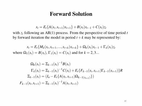
Forward Solution

xt = EtA(st,st+1)xt+1+B(st)xt−1 +C(st)zt

with zt following an AR(1) process. From the perspective of time period tby forward iteration the model in period t+ k may be represented by:

xt = EtMk(st,st+1, ...,st+k)xt+k+Ωk(st)xt−1 +Γk(st)zt

where Ω1(st) = B(st), Γ1(st) = C(st) and for k = 2,3...

Ωk(st) = Ξk−1(st)−1B(st)

Γk(st) = Ξk−1(st)−1C(st)+EtFk−1(st,st+1)Γk−1(st+1)R

Ξk−1(st) = (In−EtA(st,st+1)Ωk−1(st+1))

Fk−1(st,st+1) = Ξk−1(st)−1A(st,st+1)

11

It may be shown that given initial values, under some regularity conditionssuch as invertibility of Ξ ∀k the sequences Ωk(st) and Γk(st) are welldefined, unique and real-valued. The model is said to be forwardconvergent if the parameter matrices are convergent with k→ ∞, i.e:

limk→∞

Ωk(st) = Ω∗(st)

limk→∞

Γk(st) = Γ∗(st)

limk→∞

Fk(st,st+1) = F∗(st,st+1)

If (no-bubble condition):

limk→∞

EtMk(st,st+1, ...,st+k)xt+k= 0n×1

then the (fundamental) solution is:

xt = Ω∗(st)xt−1 +Γ

∗(st)zt

As k tends to infinity, the above condition should hold and all solutionswhere it does not should be ruled out as they are not economicallyrelevant. Thus, if the model is forward convergent and the "no-bubblecondition" is satisfied, then the above is the only relevant MSV solution.

12

Determinacy and UniquenessThe existence of the above solution alone is necessary but not sufficientcondition for determinacy, due to the volatility induced by theregime-switching feature. There may exist a non-fundamental part that isarbitrary and there may be a multiplicity of equilibria. Assuming thenon-fundamental component takes the form

wt = EtF(st,st+1)wt+1then the concept for determinacy and indeterminacy deals with interactionof the matrices when switching between states. Defining

ΨΩ∗×Ω∗ = [pijΩ∗j ⊗Ω

∗j ] and ΨF∗×F∗ = [pijF∗j ⊗F∗j ]

then, mean-square stability is characterized by

rσ(ΨΩ∗×Ω∗)< 1 rσ(ΨF∗×F∗)≤ 1

13

Solution and EstimationSolution:

xt = Ω∗(st)xt−1 +Γ

∗(st)zt

Combined with the measurement equation

Yt = Hxt +Rt

Likelihood: Kalman filter is inoperable⇒ Kim’s filterMaximization: Covariance Matrix Adaptation Evoltuion Strategy(CMA-ES)Posterior: Formed through Bayes’ rule, conditioning on the states.

p(θ,P,S|Y) = p(Y |θ,P,S)p(S |P)p(θ,P)∫p(Y |θ,P,S)p(S |P)p(P,θ)d(θ,P,S)

14

Taking the Model to DataEstonia: Real GDP growth, Consumption growth, Inflation (HICP),3-month TALIBOR (—)Europe: Real GDP growth, Inflation (HICP), 3-month EURIBOR (- -)

1996 1998 2000 2002 2004 2006 2008 2010 2012−15

−10

−5

0

5

10

4 GDP

1996 1998 2000 2002 2004 2006 2008 2010 2012−10

−5

0

5

10

4 Consumption

1996 1998 2000 2002 2004 2006 2008 2010 2012−3

−2

−1

0

1

2

3

Inflation

1996 1998 2000 2002 2004 2006 2008 2010 2012−1

−0.5

0

0.5

1

1.5

2

TALIBOR and EURIBOR

15

PriorsDist. Mean Std.Dev.

p11 Beta 0.9 0.1p22 Beta 0.9 0.1β PM 0.995 —ϕ Gamma 2 0.25θH Beta 0.75 0.1θF Beta 0.5 0.1α PM 0.5 —σ Gamma 1 1η Gamma 2 0.25δH Beta 0.5 0.15δF Beta 0.5 0.15χ Gamma 0.01 0.01ρa Beta 0.7 0.1ρµF Beta 0.7 0.1

Dist. Mean Std.Dev.ρµH Beta 0.7 0.1ρν Beta 0.7 0.1ρφ Beta 0.7 0.1cy∗ Beta 0.85 0.1cπ∗ Beta 0.85 0.1ci∗ Beta 0.85 0.1σµF IGamma 1 ∞

σµH IGamma 1 ∞

σa IGamma 1 ∞

σν IGamma 1 ∞

σφ IGamma 0.8 ∞

σy∗ IGamma 1 ∞

σπ∗ IGamma 1 ∞

σi∗ IGamma 1 ∞

16

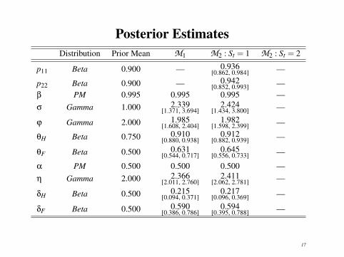
Posterior EstimatesDistribution Prior Mean M1 M2 : St = 1 M2 : St = 2

p11 Beta 0.900 — 0.936[0.862, 0.984] —

p22 Beta 0.900 — 0.942[0.852, 0.993] —

β PM 0.995 0.995 0.995 —σ Gamma 1.000 2.339

[1.371, 3.694]2.424

[1.434, 3.800] —

ϕ Gamma 2.000 1.985[1.608, 2.404]

1.982[1.598, 2.399] —

θH Beta 0.750 0.910[0.880, 0.938]

0.912[0.882, 0.939] —

θF Beta 0.500 0.631[0.544, 0.717]

0.645[0.556, 0.733] —

α PM 0.500 0.500 0.500 —η Gamma 2.000 2.366

[2.011, 2.760]2.411

[2.062, 2.781] —

δH Beta 0.500 0.215[0.094, 0.371]

0.217[0.096, 0.369] —

δF Beta 0.500 0.590[0.386, 0.786]

0.594[0.395, 0.788] —

17

Posterior EstimatesDistribution Prior Mean M1 M2 : St = 1 M2 : St = 2

χ Gamma 0.010 0.028[0.014, 0.043]

0.017[0.006, 0.029] —

σµF IGamma 1.000 1.225[0.857, 1.673]

1.159[0.799, 1.618] —

σµH IGamma 1.000 0.458[0.326, 0.620]

0.425[0.298, 0.586] —

σa IGamma 1.000 0.855[0.209, 2.358]

1.060[0.205, 3.474] —

σν IGamma 1.000 11.265[7.040, 17.150]

11.438[7.154, 17.458] —

σφ IGamma 0.800 0.472[0.406, 0.548]

0.119[0.090, 0.156]

0.665[0.533, 0.831]

σy∗ IGamma 1.000 0.684[0.592, 0.791]

0.685[0.593, 0.795] —

σπ∗ IGamma 1.000 0.375[0.321, 0.438]

0.376[0.321, 0.440] —

σi∗ IGamma 1.000 0.100[0.086, 0.116]

0.100[0.086, 0.116] —

M: -430.723 -405.5175

18

Estimated Probabilities of the High State

1996 1998 2000 2002 2004 2006 2008 20100

5

10

15

20

1996 1998 2000 2002 2004 2006 2008 20100

0.2

0.4

0.6

0.8

1

Figure: Top: Interbank interest rates, TALIBOR (—) and EURIBOR (- -).Bottom: Smoothed (u) and not-smoothed (- -) probability of σφ(st) = σφ(high).

19

2 4 6 8 10 12−1

−0.5

0

0.5Consumption

2 4 6 8 10 12−0.5

0

0.5Output

2 4 6 8 10 12−0.5

0

0.5

1Interest Rate

2 4 6 8 10 12−0.02

0

0.02

0.04Real Exchange Rate

2 4 6 8 10 12−0.05

0

0.05Terms of Trade

2 4 6 8 10 12−0.02

−0.01

0

0.01Inflation

2 4 6 8 10 12−0.04

−0.02

0

0.02Inflation Home Goods

2 4 6 8 10 12−4

−2

0

2Marginal Cost

2 4 6 8 10 120

0.5

1Net FA Position

Figure: Impulse Responses following a risk premium shock for State 1: σφ(low) (- -),State 2: σφ(high) (-.-) and the no-switching version M1 (—) .

20

Variance Decomposition and Moments

2 4 6 8 10 120

20

40

60

80

100

εy

*

επ*

εi*

εµF

εµH

εa

ενεφ

2 4 6 8 10 120

20

40

60

80

100

εy

*

επ*

εi*

εµF

εµH

εa

ενεφ

Figure: State-conditioned variance decomposition of the interest rate.

y c π i y∗ π∗ i∗

data 4.5103 4.0453 0.8323 0.4635 1.3184 0.3754 0.2169M2 : State 1 3.4937 4.1860 0.8307 0.2480 1.2781 0.4434 0.1710M2 : State 2 3.5142 4.2666 0.8291 0.6966 1.2705 0.4443 0.1708

Table: Standard deviation of the actual data and implied by the model based on 5000random simulations.

21

Robustness ChecksDifferences between the specifications:

M1: No regime shifts.M2: Switching in the volatility of the risk premium σ2

φ.

M3: Switching in the volatility in other structural shocks: σ2a, σ2

ϑ, σ2

µH, σ2

µF, σ2

φ.

M4: Switching in σ2φ

and χ.M5: Switching in σ2

φwhere the data are linearly detrended.

Estimated coefficientsM3 : St = 1 M3 : St = 2 M4 : St = 1 M4 : St = 2 M5 : St = 1 M5 : St = 2

χ 0.015[0.006, 0.028] — 0.014

[0.006, 0.025]0.024

[0.005, 0.051]0.025

[0.021, 0.030] —

σµF0.966

[0.611, 1.442]1.245

[0.810, 1.836]1.160

[0.798, 1.611] — 1.203[0.829, 1.676] —

σµH0.403

[0.275, 0.570]0.474

[0.327, 0.662]0.433

[0.312, 0.583] — 0.469[0.338, 0.629] —

σν9.569

[5.430, 15.636]10.440

[6.404, 16.143]11.473

[7.203, 17.380] — 14.568[9.090, 22.368] —

σφ0.121

[0.092, 0.160]0.673

[0.535, 0.842]0.119

[0.090, 0.156]0.680

[0.537, 0.866]0.145

[0.664, 1.175]0.887

[0.097, 0.201]

σa 0.769[0.207, 2.007]

1.040[0.212, 3.117]

0.816[0.206, 2.346] — 0.870

[0.211, 2.472] —

M: -409.2437 -405.0004 -418.835

22

Conclusion

• The Markov-switching extension is able to capture the non-linearitiesof TALIBOR

• Risk-premium shocks play negligible role during normal times, buthave more profound effects when the system is under pressure

• Successful at identifying the banking and financial crisis

• Outperforms the standard model in terms of model fit

• Allows for state-contingent analysis

• The extension is computationally more intensive

• The switching is exogenous and the number of states is ad-hoc

• The framework is flexible and unexplored, presenting manyopportunities for further research

23

0.8 10

5

10

p11

0.5 10

2

4

6

8

10

p22

1 2 30

0.5

1

1.5

ϕ

0.8 0.9 10

5

10

15

20

θH

0.4 0.6 0.80

2

4

6

θF

0 2 4 6 80

0.2

0.4

0.6σ

2 3 40

0.5

1

1.5

η

0 0.2 0.4 0.6 0.80

1

2

3

4

δH

0 0.5 10

1

2

3

δF

0 0.02 0.04 0.060

10

20

30

40

χ

0.2 0.4 0.6 0.8 10

1

2

3

ρa

0.2 0.4 0.6 0.8 10

1

2

3

4ρµF

0.2 0.4 0.6 0.8 10

1

2

3

ρµH

0.2 0.4 0.6 0.8 10

1

2

3

ρν

0 0.5 10

1

2

3

4

ρφ

0.6 0.8 10

2

4

6

cy∗

0 0.5 10

1

2

3

cπ∗

0.6 0.8 10

2

4

6

8

ci∗

0 1 2 30

0.5

1

1.5

σµF

0 0.5 10

1

2

3

4

σµH

0 5 10 150

0.2

0.4

0.6

0.8

σa

0 10 20 300

0.05

0.1

σν

0.050.10.150.20.250

5

10

15

20

σφ

0.5 10

2

4

6

σy∗

0.2 0.4 0.60

2

4

6

8

10

σπ∗

0.05 0.1 0.150

10

20

30

40

σi∗

0.5 1 1.50

1

2

3

4

σφ

Figure: Prior (dashed) and posterior (solid) distributions of M2 (no Markov-Switching).24