HAL Id: tel-01101607 https://tel.archives-ouvertes.fr/tel-01101607 Submitted on 9 Jan 2015 HAL is a multi-disciplinary open access archive for the deposit and dissemination of sci- entific research documents, whether they are pub- lished or not. The documents may come from teaching and research institutions in France or abroad, or from public or private research centers. L’archive ouverte pluridisciplinaire HAL, est destinée au dépôt et à la diffusion de documents scientifiques de niveau recherche, publiés ou non, émanant des établissements d’enseignement et de recherche français ou étrangers, des laboratoires publics ou privés. Blood flow modelling and applications to blood coagulation and atherosclerosis Alen Tosenberger To cite this version: Alen Tosenberger. Blood flow modelling and applications to blood coagulation and atherosclerosis. Mathematics [math]. Université Claude Bernard - Lyon 1 Institut Camille Jordan - CNRS UMR 5208, 2014. English. tel-01101607

Welcome message from author
This document is posted to help you gain knowledge. Please leave a comment to let me know what you think about it! Share it to your friends and learn new things together.
Transcript
HAL Id: tel-01101607https://tel.archives-ouvertes.fr/tel-01101607
Submitted on 9 Jan 2015
HAL is a multi-disciplinary open accessarchive for the deposit and dissemination of sci-entific research documents, whether they are pub-lished or not. The documents may come fromteaching and research institutions in France orabroad, or from public or private research centers.
L’archive ouverte pluridisciplinaire HAL, estdestinée au dépôt et à la diffusion de documentsscientifiques de niveau recherche, publiés ou non,émanant des établissements d’enseignement et derecherche français ou étrangers, des laboratoirespublics ou privés.
Blood flow modelling and applications to bloodcoagulation and atherosclerosis
Alen Tosenberger
To cite this version:Alen Tosenberger. Blood flow modelling and applications to blood coagulation and atherosclerosis.Mathematics [math]. Université Claude Bernard - Lyon 1 Institut Camille Jordan - CNRS UMR 5208,2014. English. �tel-01101607�
Numero d’ordre : 21 - 2014 12 Fevrier 2014
Universite Claude Bernard - Lyon 1
Institut Camille Jordan - CNRS UMR 5208
Ecole doctorale InfoMaths
Thesede l’universite de Lyon
pour obtenir le titre de
Docteur en SciencesMention : Mathematiques appliquees
presentee par
Alen Tosenberger
Blood flow modelling and applicationsto blood coagulation and atherosclerosis
These dirigee par Vitaly Volpert
preparee a l’Universite Lyon 1
Jury:
Charles Auffray DR au CNRS, EISBM, Lyon Examinateur
Jean-Claude Bordet Biologiste, Laboratoire de Recherche Examinateur
sur l’Hemophilie, Lyon 1
Ionel Sorin Ciuperca MCF, Institut Camille Jordan, Univ. Lyon 1 Examinateur
Elaine Crooks Professeur, Swansea University Examinateur
Andreas Deutsch Professeur, Technische Universit at Dresden Examinateur
Adelia Sequeira Professeur, Instituto Superior Tecnico Rapporteur
Angelique Stephanou CR au CNRS, IN3S, Grenoble Rapporteur
Vitaly Volpert DR au CNRS, Universite Lyon 1 Directeur de These

Resume
La these est consacree a la modelisation discrete et continue des ecoulements sanguinset des phenomenes connexes tels que la coagulation du sang et l’atherosclerose. Ce travailcomprend l’elaboration des modeles mathematiques et numeriques de la coagulation du sang,des simulations numeriques et l’analyse mathematique d’un modele d’inflammation chroniqueau cours d’atherosclerose. Une partie importante de la these est liee a la programmation, lamise en oeuvre et l’optimisation des codes numeriques.
La partie principale de la these concerne la modelisation de la coagulation du sang invivo tenant compte des ecoulements sanguins, les reactions biochimiques dans le plasmaet l’agregation de plaquettes. La nouveaute principale de ce travail est l’elaboration d’unmodele hybride (discret-continu) de la coagulation du sang et de la formation de caillotsanguin dans le flux. La partie discrete du modele est basee sur la methode particulaireappelee la Dynamique des Particules Dissipatives (DPD). En raison de sa nature discrete, lamethode DPD nous permet de decrire des cellules sanguines individuelles. Cette methodeest utilisee pour la modelisation de l’ecoulement du plasma sanguin, des plaquettes et deleur agregation. La partie continue du modele utilise les equations aux derivees partiellespour decrire les concentrations de substances biochimiques dans le plasma et leurs reactionslors de la coagulation. Plusieurs aspects de la coagulation ont ete etudies: l’agregationde plaquettes et son interaction avec les reactions biochimiques de coagulation, l’influencede la vitesse d’ecoulement sur le developpement d’un caillot sanguin ainsi que commentla croissance du caillot s’arrete. Le modele a montre l’importance de l’interaction entrel’agregation de plaquettes et les reactions de coagulation. La vitesse d’ecoulement est faiblea l’interieur des caillots, ce qui permet de declencher la cascade de coagulation et de renforcerl’agregat accroissant par la formation du polymere de fibrine. La pression exercee par le fluxsanguin enleve les parties exterieures du caillot et arrete finalement la croissance.
La partie theorique de la these est consacree a l’analyse mathematique d’un modeled’inflam-mation chronique liee a l’atherosclerose. Auparavant, il a ete montre que l’inflammationse propage comme une onde de reaction-diffusion dont les caracteristiques dependent duniveau du mauvais cholesterol dans le sang. Dans cette these, nous etudions un modeledecrivant la propagation d’une onde de reaction-diffusion dans le cas 2D avec des conditionsaux limites non-lineaires. Nous utilisons la methode de Leray-Schauder et des estimations apriori des solutions afin de prouver l’existence d’ondes dans le cas bistable.
Les simulations numeriques realisees dans le cadre de cette these impliquent l’elaborationdes algorithmes numeriques pour les modeles mathematiques et le developpement des logi-ciels. Vu le fait que les simulations numeriques ont ete couteuse en temps de calcul, des effortsconsiderables ont ete consacres a la parallelisation des logiciels et a leur optimisation.
Mots-cles : modeles hybrides, Dissipative Particle Dynamics, equations aux derivees par-tielles, coagulation du sang, developpement de caillot sanguin, atherosclerose.
Abstract
The thesis is devoted to discrete and continuous modelling of blood flows and relatedphenomena such as blood coagulation and atherosclerosis. It includes the development ofmathematical and numerical models of blood coagulation, numerical simulations and themathematical analysis of a model problem of chronic inflammation during atherosclerosis.An important part of the thesis is related to programming, implementation and optimizationof numerical codes.
The main part of the thesis concerns modelling of blood coagulation in vivo which takesinto account blood flows, biochemical reactions in plasma and platelet aggregation. Themain novelty of this work is the development of a hybrid (discrete-continuous) model ofblood coagulation and clot formation in flow. The discrete part of the model is based on aparticle method called Dissipative Particle Dynamics (DPD). Due to the discrete nature ofthe DPD method, it allows the description of individual blood cells. This method is usedto model blood plasma flow, platelets suspended in it and platelet aggregation. The con-tinuous part of the model is based on partial differential equations for the concentrations ofbiochemical substances in the blood plasma and their reactions during blood coagulation.Several aspects of blood coagulation in flow were studied: platelet aggregation and its in-teraction with coagulation pathways, influence of the flow speed on the clot development, apossible mechanism by which clot stops growing. The model showed the importance of theinteraction between platelet aggregation and coagulation pathways. Since the flow velocityis small inside of the platelet clot, it is possible for the coagulation cascade to begin and toreinforce the growing aggregate by the formation of a fibrin network. The pressure from theblood flow removes the outer parts of the platelet clot and eventually stops it growth.
The theoretical part of the thesis is devoted to the mathematical analysis of a model ofchronic inflammation related to atherosclerosis. Previously it was shown that inflammationpropagates as a reaction-diffusion wave whose properties depend on the level of bad choles-terol in blood. In this thesis we study a model problem which describes the propagation ofa reaction-diffusion wave in the 2D case with non-linear boundary conditions. We use theLeray-Schauder method and a priori estimates of solutions in order to prove the existence ofwaves in the bistable case.
Numerical simulations carried out in the framework of this thesis were based on thenumerical implementation of the corresponding models and on the software development.Since the numerical simulations were computationally expensive, a substantial effort wasdirected to software parallelization and optimization.
Key words: hybrid models, Dissipative Particle Dynamics, partial differential equations,blood coagulation, clot growth, atherosclerosis.
Acknowledgements
I would like to express my deepest gratitude to my supervisor Vitaly Volpert for hisclear and comprehensive guidance and unreserved support throughout my PhD.
I would also like to extend my sincere appreciation to Nikolay Bessonov from the Insti-tute of Mechanical Engineering Problems in Saint Petersburg for the invaluable advise andideas on numerical methods.
My deep appreciation is extended to Fazly Ataullakhanov, Mikhail Panteleev and AlexeyTokarev from the National Research Center for Haematology in Moscow for the valuablecollaboration and for providing the insight into the most recent advancements in the exper-imental research of blood coagulation.
I am very grateful to the reporters Adelia Sequeira and Angelique Stephanou, and thejury members Charles Auffray, Jean-Claude Bordet, Ionel Sorin Ciuperca, Elaine Crooksand Andreas Deutsch, for coming to Lyon and participating in the thesis defence, as well asfor their exhaustive questions and comments.
I would also like to give special thanks to my colleagues from the INRIA Dracula team inLyon, for their kind support and collegiality during my PhD, especially to Mostafa Adimy,Samuel Bernard, Fabien Crauste, Olivier Grandrillon, Thomas Lepoutre, Laurent Pujo-Menjouet and Caroline Lothe.
Moreover, I would like to extend my gratitude to Grigory Panasenko from Universitede Saint-Etienne and Jean-Pierre Loheac from Ecole Centrale de Lyon for providing severalopportunities to present my work.
Last but not least, I would like to thank my wife Mathea, my family and my friends forsharing both the good and the bad moments, for their love and encouragement.

i
Contents
1 Introduction 11.1 Blood flow . . . . . . . . . . . . . . . . . . . . . . . . . . . . . . . . . . . . . 1
1.1.1 Biological background . . . . . . . . . . . . . . . . . . . . . . . . . . 11.1.2 Modelling . . . . . . . . . . . . . . . . . . . . . . . . . . . . . . . . . 4
1.2 Blood coagulation . . . . . . . . . . . . . . . . . . . . . . . . . . . . . . . . . 91.2.1 Biological background . . . . . . . . . . . . . . . . . . . . . . . . . . 91.2.2 Modelling . . . . . . . . . . . . . . . . . . . . . . . . . . . . . . . . . 13
1.3 Atherosclerosis . . . . . . . . . . . . . . . . . . . . . . . . . . . . . . . . . . 151.3.1 Biological background . . . . . . . . . . . . . . . . . . . . . . . . . . 151.3.2 Modelling . . . . . . . . . . . . . . . . . . . . . . . . . . . . . . . . . 17
1.4 Main results of the thesis . . . . . . . . . . . . . . . . . . . . . . . . . . . . . 21
2 Dissipative Particle Dynamics 232.1 Description . . . . . . . . . . . . . . . . . . . . . . . . . . . . . . . . . . . . 232.2 2D Poiseuille flow . . . . . . . . . . . . . . . . . . . . . . . . . . . . . . . . . 26
2.2.1 Measurements . . . . . . . . . . . . . . . . . . . . . . . . . . . . . . . 262.2.2 Physical parameters in 2D . . . . . . . . . . . . . . . . . . . . . . . . 282.2.3 Calculating viscosity . . . . . . . . . . . . . . . . . . . . . . . . . . . 292.2.4 Calculating wall shear rate . . . . . . . . . . . . . . . . . . . . . . . . 33
2.3 Boundary conditions . . . . . . . . . . . . . . . . . . . . . . . . . . . . . . . 332.3.1 Hard boundary conditions . . . . . . . . . . . . . . . . . . . . . . . . 342.3.2 Semi-periodic boundary conditions . . . . . . . . . . . . . . . . . . . 352.3.3 Estimated boundary conditions . . . . . . . . . . . . . . . . . . . . . 362.3.4 Measured boundary conditions . . . . . . . . . . . . . . . . . . . . . . 392.3.5 Mirror boundary conditions . . . . . . . . . . . . . . . . . . . . . . . 412.3.6 Enforced boundary conditions . . . . . . . . . . . . . . . . . . . . . . 422.3.7 Particle generation area . . . . . . . . . . . . . . . . . . . . . . . . . 42
2.4 Erythrocyte model . . . . . . . . . . . . . . . . . . . . . . . . . . . . . . . . 442.4.1 Capillary flow . . . . . . . . . . . . . . . . . . . . . . . . . . . . . . . 462.4.2 3D model . . . . . . . . . . . . . . . . . . . . . . . . . . . . . . . . . 46
3 Discrete model of platelet aggregation in flow 49
ii CONTENTS
3.1 Description . . . . . . . . . . . . . . . . . . . . . . . . . . . . . . . . . . . . 493.2 Time dependent platelet adhesion force . . . . . . . . . . . . . . . . . . . . . 503.3 Results . . . . . . . . . . . . . . . . . . . . . . . . . . . . . . . . . . . . . . . 51
3.3.1 Constant coefficient of adhesion force strength . . . . . . . . . . . . . 523.3.2 Time dependent platelet adhesion force . . . . . . . . . . . . . . . . . 533.3.3 Arrest of clot growth . . . . . . . . . . . . . . . . . . . . . . . . . . . 54
4 Hybrid model of blood coagulation in flow 574.1 One equation model . . . . . . . . . . . . . . . . . . . . . . . . . . . . . . . 57
4.1.1 Fibrin concentration . . . . . . . . . . . . . . . . . . . . . . . . . . . 584.1.2 Clot growth . . . . . . . . . . . . . . . . . . . . . . . . . . . . . . . . 59
4.2 Three equations model . . . . . . . . . . . . . . . . . . . . . . . . . . . . . . 634.2.1 Coagulation pathway model . . . . . . . . . . . . . . . . . . . . . . . 634.2.2 Platelet aggregation . . . . . . . . . . . . . . . . . . . . . . . . . . . 674.2.3 Parameters . . . . . . . . . . . . . . . . . . . . . . . . . . . . . . . . 684.2.4 Model behaviour . . . . . . . . . . . . . . . . . . . . . . . . . . . . . 714.2.5 PDE parameters . . . . . . . . . . . . . . . . . . . . . . . . . . . . . 744.2.6 Platelet bond strength . . . . . . . . . . . . . . . . . . . . . . . . . . 764.2.7 Flow velocity influence . . . . . . . . . . . . . . . . . . . . . . . . . . 79
5 Mathematical analysis of a model problem for atherosclerosis 815.1 Introduction . . . . . . . . . . . . . . . . . . . . . . . . . . . . . . . . . . . . 815.2 Formulation of the problem . . . . . . . . . . . . . . . . . . . . . . . . . . . 825.3 Solutions in the cross-section . . . . . . . . . . . . . . . . . . . . . . . . . . . 84
5.3.1 General case . . . . . . . . . . . . . . . . . . . . . . . . . . . . . . . . 845.3.2 Constant solutions . . . . . . . . . . . . . . . . . . . . . . . . . . . . 86
5.4 Property of the operators . . . . . . . . . . . . . . . . . . . . . . . . . . . . . 875.4.1 Fredholm property . . . . . . . . . . . . . . . . . . . . . . . . . . . . 875.4.2 Properness and topological degree . . . . . . . . . . . . . . . . . . . . 89
5.5 A priori estimates . . . . . . . . . . . . . . . . . . . . . . . . . . . . . . . . . 895.5.1 Auxiliary results . . . . . . . . . . . . . . . . . . . . . . . . . . . . . 895.5.2 Functionalization of the parameter . . . . . . . . . . . . . . . . . . . 915.5.3 Estimates of solutions . . . . . . . . . . . . . . . . . . . . . . . . . . 92
5.6 Leray-Schauder method . . . . . . . . . . . . . . . . . . . . . . . . . . . . . 945.6.1 Model problem . . . . . . . . . . . . . . . . . . . . . . . . . . . . . . 945.6.2 Wave existence . . . . . . . . . . . . . . . . . . . . . . . . . . . . . . 96
Conclusion and Perspectives 101
Publications 103
Bibliography 105

CONTENTS iii
6 Appendix A - Hybrid model implementation 1176.1 Code structure . . . . . . . . . . . . . . . . . . . . . . . . . . . . . . . . . . 1176.2 Optimization . . . . . . . . . . . . . . . . . . . . . . . . . . . . . . . . . . . 122
6.2.1 Boxing scheme . . . . . . . . . . . . . . . . . . . . . . . . . . . . . . 1226.2.2 Velocity profile smoothing . . . . . . . . . . . . . . . . . . . . . . . . 1236.2.3 Dual time steps . . . . . . . . . . . . . . . . . . . . . . . . . . . . . . 1236.2.4 Additional integration scheme for the equations of motion in DPD . . 1246.2.5 Parallelism - OpenMP, GPGPU . . . . . . . . . . . . . . . . . . . . . 126
6.3 Numerical method for solving reaction-diffusion-advection equation . . . . . 1296.4 Proof of lemma 5.7 . . . . . . . . . . . . . . . . . . . . . . . . . . . . . . . . 133

1
Chapter 1
Introduction
The thesis is devoted to blood flow modelling with applications to blood coagulation andatherosclerosis. In this introduction these physiological processes and the state of the art intheir mathematical modelling will be described. The introduction finishes with the presen-tation of the main results of the thesis.
1.1 Blood flow
1.1.1 Biological background
The blood is one of the largest organs in the body, which performs the essential functionof delivering oxygen and nutrients to all tissues and cells, as well as of taking away themetabolic waste products. As the cardiovascular system spans through the whole body,blood has the role of supporting the function of all other body tissues. By transportingantibodies the blood also makes it possible for the organism to react to and fight infections.Other functions include coagulation, which is a body’s self-repair mechanism, messengerfunctions, by transporting hormones and signalling tissue damage, and regulation of bodypH and temperature. Because of its functions and presence in all tissues of the body, bloodand cardiovascular system are involved with the most pathological events and the relatedhealing approaches, either as a cause of a disease, as a tissue that can be involved in variousways with the effects of the disease, as a way to administer the medicine and to counteract orcure the disease. Due to its important role and involvement in body functions and diseases,but also due to the easy sampling of blood, it has been in a focus of numerous medical,biological, chemical, physical, mathematical and pharmaceutical studies, and is probably oneof the most intensively studied organs. Histologically, blood is considered to be a connectingtissue. However, being a fluid it differs largely from other connecting tissues.
2 1.1. BLOOD FLOW
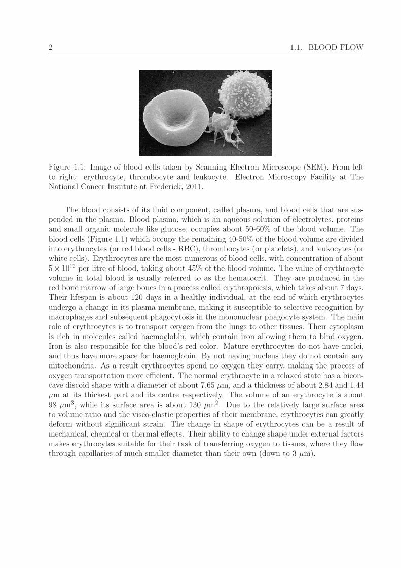
Figure 1.1: Image of blood cells taken by Scanning Electron Microscope (SEM). From leftto right: erythrocyte, thrombocyte and leukocyte. Electron Microscopy Facility at TheNational Cancer Institute at Frederick, 2011.
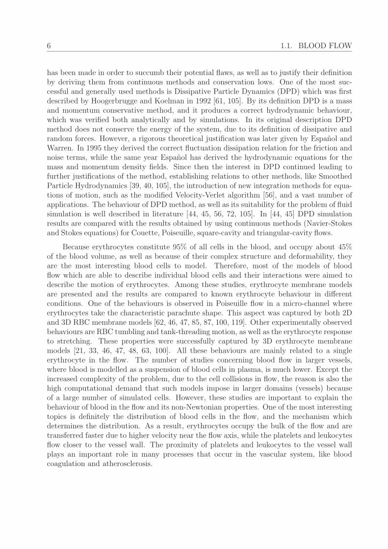
The blood consists of its fluid component, called plasma, and blood cells that are sus-pended in the plasma. Blood plasma, which is an aqueous solution of electrolytes, proteinsand small organic molecule like glucose, occupies about 50-60% of the blood volume. Theblood cells (Figure 1.1) which occupy the remaining 40-50% of the blood volume are dividedinto erythrocytes (or red blood cells - RBC), thrombocytes (or platelets), and leukocytes (orwhite cells). Erythrocytes are the most numerous of blood cells, with concentration of about5× 1012 per litre of blood, taking about 45% of the blood volume. The value of erythrocytevolume in total blood is usually referred to as the hematocrit. They are produced in thered bone marrow of large bones in a process called erythropoiesis, which takes about 7 days.Their lifespan is about 120 days in a healthy individual, at the end of which erythrocytesundergo a change in its plasma membrane, making it susceptible to selective recognition bymacrophages and subsequent phagocytosis in the mononuclear phagocyte system. The mainrole of erythrocytes is to transport oxygen from the lungs to other tissues. Their cytoplasmis rich in molecules called haemoglobin, which contain iron allowing them to bind oxygen.Iron is also responsible for the blood’s red color. Mature erythrocytes do not have nuclei,and thus have more space for haemoglobin. By not having nucleus they do not contain anymitochondria. As a result erythrocytes spend no oxygen they carry, making the process ofoxygen transportation more efficient. The normal erythrocyte in a relaxed state has a bicon-cave discoid shape with a diameter of about 7.65 μm, and a thickness of about 2.84 and 1.44μm at its thickest part and its centre respectively. The volume of an erythrocyte is about98 μm3, while its surface area is about 130 μm2. Due to the relatively large surface areato volume ratio and the visco-elastic properties of their membrane, erythrocytes can greatlydeform without significant strain. The change in shape of erythrocytes can be a result ofmechanical, chemical or thermal effects. Their ability to change shape under external factorsmakes erythrocytes suitable for their task of transferring oxygen to tissues, where they flowthrough capillaries of much smaller diameter than their own (down to 3 μm).
1.1. BLOOD FLOW 3
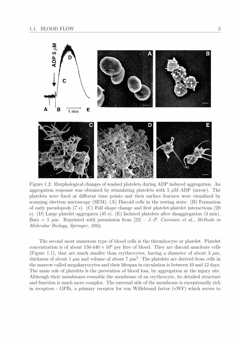
Figure 1.2: Morphological changes of washed platelets during ADP induced aggregation. Anaggregation response was obtained by stimulating platelets with 5 μM ADP (arrow). Theplatelets were fixed at different time points and their surface features were visualized byscanning electron microscopy (SEM). (A) Discoid cells in the resting state. (B) Formationof early pseudopods (7 s). (C) Full shape change and first platelet-platelet interactions (20s). (D) Large platelet aggregates (45 s). (E) Isolated platelets after disaggregation (3 min).Bars = 1 μm. Reprinted with permission from [22] – J.-P. Cazenave et al., Methods inMolecular Biology, Springer, 2004.
The second most numerous type of blood cells is the thrombocyte or platelet. Plateletconcentration is of about 150-440 × 109 per litre of blood. They are discoid anucleate cells(Figure 1.1), that are much smaller than erythrocytes, having a diameter of about 3 μm,thickness of about 1 μm and volume of about 7 μm3. The platelets are derived from cells inthe marrow called megakaryocytes and their lifespan in circulation is between 10 and 12 days.The main role of platelets is the prevention of blood loss, by aggregation at the injury site.Although their membranes resemble the membrane of an erythrocyte, its detailed structureand function is much more complex. The external side of the membrane is exceptionally richin receptors - GPIb, a primary receptor for von Willebrand factor (vWF) which serves to
4 1.1. BLOOD FLOW
mediate the initial adhesion between the platelets, GPIIb/IIIa which acts as a receptor forfibrinogen and vWF and others like receptors for ADP and thrombin which also play a rolein the platelet aggregation. Except receptors that are present on the surface of a platelet, asecond mechanism exists to facilitate the platelet aggregation (Figure 1.2). In this process,known as platelet activation, platelets undergo a shape change from the initial discoid shapeto a more spherical shape with pseudopodia (stellate shape). The drastic change in shapeincreases the surface of platelets and thus facilitates surface adhesion interactions. In theearly stages of activation the shape change is still reversible, while after they have undergonethe full transformation, the change becomes irreversible.
The least numerous type of blood cells is the leukocyte, with a concentration of about5 × 109 per litre of blood. Together with platelets, leukocytes account for 1% of the totalblood volume. They are roughly spherical in shape with a diameter ranging from 7 to 22μm. Their function is to fight infection in the body through both the destruction of bacteriaand viruses, and the formation of antibodies and sensitized lymphocytes. Leukocytes areproduced in the bone marrow and partially in the lymph tissue. While they are constantlypresent in a healthy blood stream, about three times more leukocytes are stored in the bonemarrow, from where they can be rapidly deployed to different parts of the organism in acase of infection or inflammation. Morphologically, there are five different types of leuko-cytes, specialized for specific and non-specific reactions on foreign materials in the organism.The five types of leukocytes are: neutrophils, eosinophils, basophils, monocytes and lym-phocytes. The first three groups, collectively known as “granulocytes” make 50-75% of thetotal number of circulating leukocytes. Granulocytes are responsible for a rapid defensiveresponse upon detection of foreign materials in the organism. Monocytes and lymphocytesare responsible for a slower but more powerful defensive reaction. While lymphocytes areresponsible for antigen-specific immune responses, the monocytes have a non-specific phago-cytic function.
1.1.2 Modelling
Because of its importance, blood was extensively studied on both the macro and the microlevel. A significant part of these studies included modelling of blood flows, in order to investi-gate blood flow mechanical and bio-chemical properties, as well as blood related phenomenalike blood coagulation or atherosclerosis.
The blood flow characteristics come from three involved parts. The first part are bloodvessels that influence the blood flow by their type, size and elastic properties. There are threemain types of blood vessels: arteries, veins and capillaries. Arteries and veins are larger bloodvessels, which carry the blood away and towards the heart respectively, while capillaries aresmaller blood vessels which enable the exchange of water and chemicals between the bloodand tissues. Arteries and veins contain a muscle layer which allows them to regulate theirinner diameter by its contraction. The second part that influences the blood flow is the
1.1. BLOOD FLOW 5
heartbeat, i.e. the heart produces a pulsatile flow by its periodic contractions. This resultsin oscillations in the flow speed and pressure between heartbeats. The third part is blood,which composition is described in the previous section. All of the three parts - blood vessels,heartbeat, blood - are very complex systems and are thus in most models described withdifferent level of details, usually having only one system in the focus of a study.
As a fluid blood is incompressible and has non-Newtonian properties, i.e. its viscositydepends on the shear rate. Although this property of blood comes from the properties oferythrocytes and other blood cells, which account for about 45% of blood volume, on themacro scale blood is usually modelled as a homogeneous fluid. In the classical approachesblood flow is usually described by partial differential equations, commonly Navier-Stokesequations [20, 31, 50, 52, 115], which, based on the properties of the fluid (density, viscos-ity), pressure or body force, and the given domain, give the corresponding velocity field.Furthermore, continuous approaches use differential equations also to describe phenomenarelated to blood flows. Concentrations of various substances are modelled with partial dif-ferential equations able to describe their diffusion and advection in the blood. Similarly,the blood cells are considered in terms of concentrations, and their motion is described alsovia diffusion and advection [113, 136]. The main disadvantage of continuous approaches isthat they do not describe the interaction between individual blood cells in the flow. Theseinteractions have an important impact on properties of the blood (blood flow), but they alsoplay an essential role in many blood flow related phenomena and diseases. Nevertheless, thesignificance of continuous models is tremendous, as they give a mathematically well basedand physically precise description of fluid behaviour related to its physical properties andprovide a precise description of behaviour of other substances in the fluid.
Discrete models enable a description of individual cells and their interactions. However,the hydrodynamic properties in such models either have to be proven by a strict mathe-matical derivation from conservation laws and continuous hydrodynamic equations, or theyhave to be verified by comparison with accurate continuous models. A classical example ofa discrete method is Molecular Dynamics (MD) [2, 60, 103], where the simulated medium isdecomposed on particles represented by their centre of mass. The motion of the system isthen determined by a pair-wise force acting between particles. In MD a single particle usuallydescribes an atom or molecule. Hence, this method is not very efficient for studying problemson a larger scale (ex. blood flow). However, many other discrete methods were developedor adapted in order to describe complex fluids in larger domains [2, 24, 34, 55, 105, 137].Usually such methods are referred to as meso-scale methods, because they model the com-plex structure of a fluid on a micro-scale, while they are still efficient for studying its effectson a macro-scale. This approach is called “coarse-graining” - the process of representing asystem with fewer degrees of freedom than those actually present in the system [39, 105].Many of such methods are not strictly mathematically derived but are rather constructed inorder to satisfy certain conservation laws and symmetries that are considered to be essentialfor the observed phenomena. Since the interest in this area began thirty years ago, a lot ofmeso-scale methods and their specialised variants have been developed and a lot of effort
6 1.1. BLOOD FLOW
has been made in order to succumb their potential flaws, as well as to justify their definitionby deriving them from continuous methods and conservation lows. One of the most suc-cessful and generally used methods is Dissipative Particle Dynamics (DPD) which was firstdescribed by Hoogerbrugge and Koelman in 1992 [61, 105]. By its definition DPD is a massand momentum conservative method, and it produces a correct hydrodynamic behaviour,which was verified both analytically and by simulations. In its original description DPDmethod does not conserve the energy of the system, due to its definition of dissipative andrandom forces. However, a rigorous theoretical justification was later given by Espanol andWarren. In 1995 they derived the correct fluctuation dissipation relation for the friction andnoise terms, while the same year Espanol has derived the hydrodynamic equations for themass and momentum density fields. Since then the interest in DPD continued leading tofurther justifications of the method, establishing relations to other methods, like SmoothedParticle Hydrodynamics [39, 40, 105], the introduction of new integration methods for equa-tions of motion, such as the modified Velocity-Verlet algorithm [56], and a vast number ofapplications. The behaviour of DPD method, as well as its suitability for the problem of fluidsimulation is well described in literature [44, 45, 56, 72, 105]. In [44, 45] DPD simulationresults are compared with the results obtained by using continuous methods (Navier-Stokesand Stokes equations) for Couette, Poiseuille, square-cavity and triangular-cavity flows.
Because erythrocytes constitute 95% of all cells in the blood, and occupy about 45%of the blood volume, as well as because of their complex structure and deformability, theyare the most interesting blood cells to model. Therefore, most of the models of bloodflow which are able to describe individual blood cells and their interactions were aimed todescribe the motion of erythrocytes. Among these studies, erythrocyte membrane modelsare presented and the results are compared to known erythrocyte behaviour in differentconditions. One of the behaviours is observed in Poiseuille flow in a micro-channel whereerythrocytes take the characteristic parachute shape. This aspect was captured by both 2Dand 3D RBC membrane models [62, 46, 47, 85, 87, 100, 119]. Other experimentally observedbehaviours are RBC tumbling and tank-threading motion, as well as the erythrocyte responseto stretching. These properties were successfully captured by 3D erythrocyte membranemodels [21, 33, 46, 47, 48, 63, 100]. All these behaviours are mainly related to a singleerythrocyte in the flow. The number of studies concerning blood flow in larger vessels,where blood is modelled as a suspension of blood cells in plasma, is much lower. Except theincreased complexity of the problem, due to the cell collisions in flow, the reason is also thehigh computational demand that such models impose in larger domains (vessels) becauseof a large number of simulated cells. However, these studies are important to explain thebehaviour of blood in the flow and its non-Newtonian properties. One of the most interestingtopics is definitely the distribution of blood cells in the flow, and the mechanism whichdetermines the distribution. As a result, erythrocytes occupy the bulk of the flow and aretransferred faster due to higher velocity near the flow axis, while the platelets and leukocytesflow closer to the vessel wall. The proximity of platelets and leukocytes to the vessel wallplays an important role in many processes that occur in the vascular system, like bloodcoagulation and atherosclerosis.
1.1. BLOOD FLOW 7
Figure 1.3: Left: a biconcave shape of RBC (Centers for Disease Control and Prevention,Public Health Image Library, Janice Carr). Right: Erythrocyte dimensions. Reprinted withpermission from [104] – A.M. Robertson et al., Oberwolfach Seminars, Birkhauser VerlagBasel, 2008.
Computational studies have been done in order to simulate this feature of blood flowwhich corresponds to the experimental observation of concentration of RBCs at the flow axis.Tsubota et al. [119] presented a two-dimensional particle model for blood flows between twoparallel rigid plates. The moving particle semi-explicit (MPS) method was used to analysethe blood plasma flow. RBC was modelled as a deformable elastic membrane consisting ofparticles with the elastic energy depending on the distance between them, the angle betweenthe neighbouring elements and the conservation of the membrane area. The simulation re-sults demonstrated that RBCs concentrate near the flow axis forming the cell free layer nearthe boundaries. In a more recent work of Zhang et al. [140] another approach is used.Two-dimensional blood flow is simulated using the immersed-boundary lattice Boltzmannalgorithm. Following Bagchi [12], RBCs are modelled as two-dimensional deformable bicon-cave membranes, while inter-cellular interactions are modelled using the Morse potential. Inaddition to the presence of the cell free layer it is shown that this layer thickness increaseswith cell deformability. In their work a known effect of erythrocytes migration toward theflow axis was observed, while platelets and their behaviour were not considered. AlMomaniet al. [3] used the computational fluid dynamics (CFD) model to perform micro-scale simu-lations of platelet-RBC interactions in a shear flow. RBCs are assumed to be incompressibleelliptical particles that retain elliptical shape during deformation by imposed shear stressesand platelets are assumed to be rigid particles of circular shape. The interaction betweenneighbouring particles is due to repulsive forces from a “soft” potential. It is shown thatthe concentration of platelets increases near the boundary, while erythrocytes are locatednear the flow axis. It was also found that the platelets behaviour is affected by the relativedifferences in the size of platelets and RBCs, but not by the differences in shape. Valuesof hematocrit were set to be 5%, 10% and 15%, which are lower than the normal hema-tocrit level in blood. Furthermore, it was observed that the migratory effect is absent atlow hematocrit values (e.g., Ht = 5%), but occurs at higher values (e.g., Ht = 10%) and
8 1.1. BLOOD FLOW
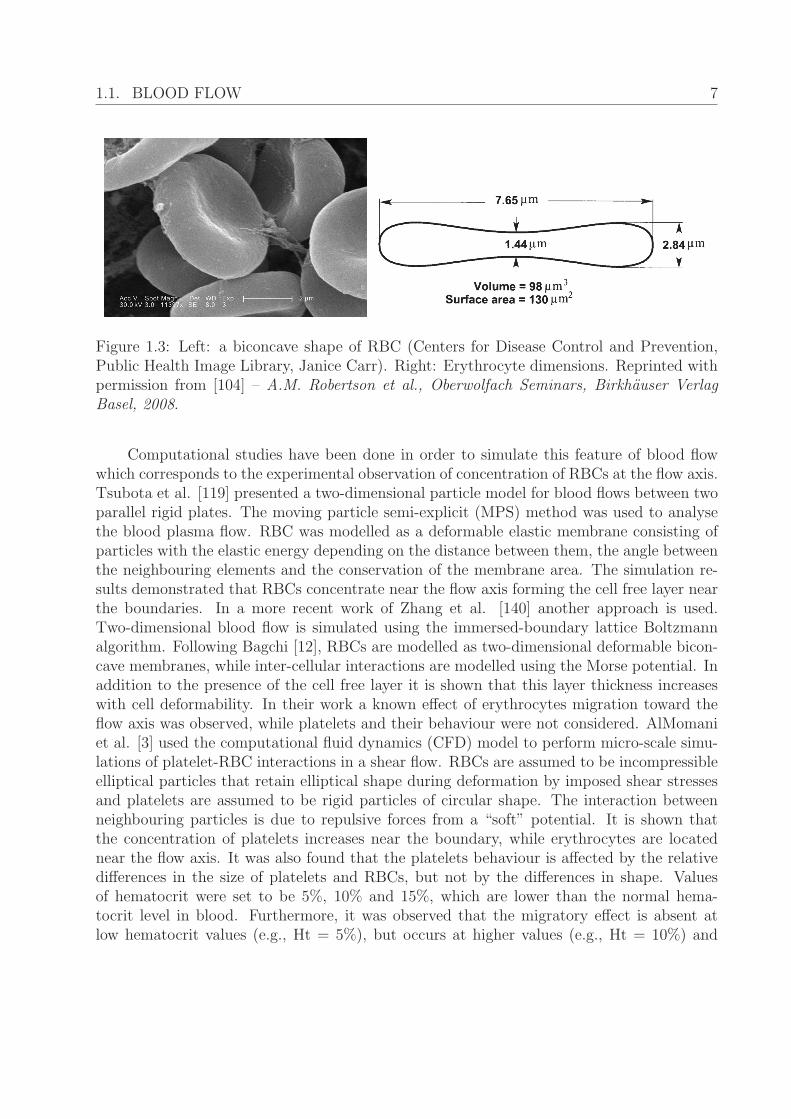
becomes more evident as the hematocrit value increases. Another study [29] was devoted toa two-dimensional numerical investigation of the lateral platelet motion induced by RBCs.In that study a combination of the lattice Boltzmann method for fluid motion and ImmersedBoundary method was used for the implementation of interaction between fluid and elasticobjects suspended in or in contact with the fluid. A deformable elastic RBCs membrane wasmodelled following the Skalak [109] approach, while platelets were modelled as approximatelyrigid circular objects. Simulations were carried out for the following values of hametocrit:0%, 20% and 40%. In the case of the RBC absence there was a negligible amount of lateralmotion, however it was clearly shown that a near-wall increase in the platelet concentrationoccurs rapidly (within the first 400 ms) at both 20% and 40% hematocrits. In [15, 16] athree-dimensional discrete model that includes the simulation of blood as a suspension of ery-throcytes and platelets in the blood plasma was used. Dissipative Particle Dynamics (DPD)method was used to carry out simulations of blood flow in a cylindrical vessel. RBCs weremodelled as elastic highly deformable membranes. In contrast with [44], where a platelet ismodelled as a rigid or almost rigid body, platelets were considered as elastic, although nearspherical, membranes. The work investigates interaction between RBCs and platelets in flowand their distribution in the cross section of the vessel.
Figure 1.4: Left: Erythrocytes (larger cells) and platelets (smaller cells), suspended in bloodplasma (not shown), in a flow through a 3D cylindrical channel, simulated by DPD method.Middle: Erythrocytes and a leukocyte (white cell) in a flow. Right: The distribution oferythrocytes and platelets as the function of distance from the flow axis. Reprinted withpermission from [16] – N. Bessonov et al., Mathematical Modelling of Natural Phenomena,Cambridge University Press, 2014.
The distribution of platelets in flow, as shown in Figure 1.4, makes platelets naturallyavailable at the site where they are most needed in the case of a vessel injury. Hence, thepositioning of platelets makes the response of the organism to stop the bleeding, throughthe processes of platelet aggregation and blood coagulation, much more effective. Similarly,the distribution of leukocytes, which roll next to the vessel wall, makes it possible for them
1.2. BLOOD COAGULATION 9
to exit the vessel, by the process of extravasation, and to go to the site of tissue damageor infection. This mechanism is also relevant for atherosclerosis, as monocytes are recruitedfrom the blood flow and integrated in the vessel wall intima in a response to the vessel wallinflammation.
1.2 Blood coagulation
1.2.1 Biological background
Hemostasis is a protective physiological mechanism that functions to stop bleeding upon vas-cular injury by sealing the wound with aggregates of specialized blood cells, platelets, andwith gelatinous fibrin clots. Disorders of this system are the leading immediate cause of mor-tality and morbidity in the modern society. The most prominent of them is thrombosis, theintravascular formation of clots that obstruct the blood flow in vessels. The life-threateningclot formation is an ubiquitous complication or even a cause of numerous diseases and condi-tions such as atherosclerosis, trauma, stroke, infarction, cancer, sepsis and others. To provideonly one example, 70% of sudden cardiac deaths are due to thrombosis [32] and they annu-ally kill approximately 400 000 people in the United States only [88]. The development ofthrombosis diagnostics and antithrombotic therapy is hampered by the incredible complexityof the hemostatic system comprising thousands of biochemical reactions of coagulation andplatelet signalling that occur in the presence of the spatial heterogeneity, cell reorganizationand blood flow. The most promising pathway to resolving this problem is systems biology, anovel multidisciplinary science aimed at quantitative analysis and understanding of complexbiological systems with the help of high-throughput experimental methods and computa-tional modelling approaches. During the last 20 years, the hemostasis system was a subjectof intense interest in this field; reviews are available that describe these theoretical studies ofblood coagulation [9, 93] and platelet-dependent hemostasis and thrombosis [93, 130, 135]. Inrecent years, computational modelling of coagulation has become a very widely used tool forinvestigating the mechanisms of drug action, optimization of therapy, analysis of drug-druginteraction at early stages (e.g. see recent examples for direct factor Xa inhibitors, novelanti-TFPI aptamer and recombinant activated factor VIII [90, 96, 108]). However, numerousproblems remain. There is currently no mathematical model that could adequately accountfor all innumerable aspects of thrombosis and hemostasis; even the best ones usually usevery unreliable assumptions about platelets, biochemistry and hydrodynamics. Finding asolution to these problems requires close cooperation between specialists in the hemostasisfield and those in computational mathematics.
The two principal components of hemostasis are: i) platelets, specialized cells thatadhere to the damaged tissue and form a primary plug reducing blood loss; ii) blood coagu-lation, a complex reaction network that turns fluid plasma into a solid fibrin gel to completelyseal the wound. Maintaining the delicate balance between the fluid and the solid states of
10 1.2. BLOOD COAGULATION
blood is not simple, and a lion’s share among the causes of mortality and morbidity in themodern society belongs to hemostatic disorders. The leading one is thrombosis, intravascularformation of platelet-fibrin clots that obstruct the blood flow in vessels. The major obstaclefor the prevention and treatment of thrombosis is the insufficient knowledge of its regulationmechanisms. Platelet aggregation and blood coagulation are extremely complex processes.Attachment of platelets and their accumulation into a clot is regulated by mechanical inter-actions with erythrocytes and the vessel wall, by numerous chemical agents such as thrombin,or ADP, or prostaglandins, or collagen, as well as by an enormous network of intracellularsignalling. Blood coagulation is only marginally simpler, including some fifty proteins thatinteract with each other and with the blood or vascular cells in approximately two hundredreactions in the presence of flow and diffusion.
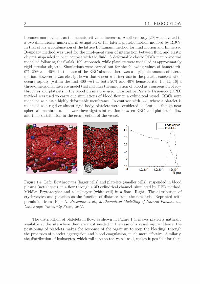
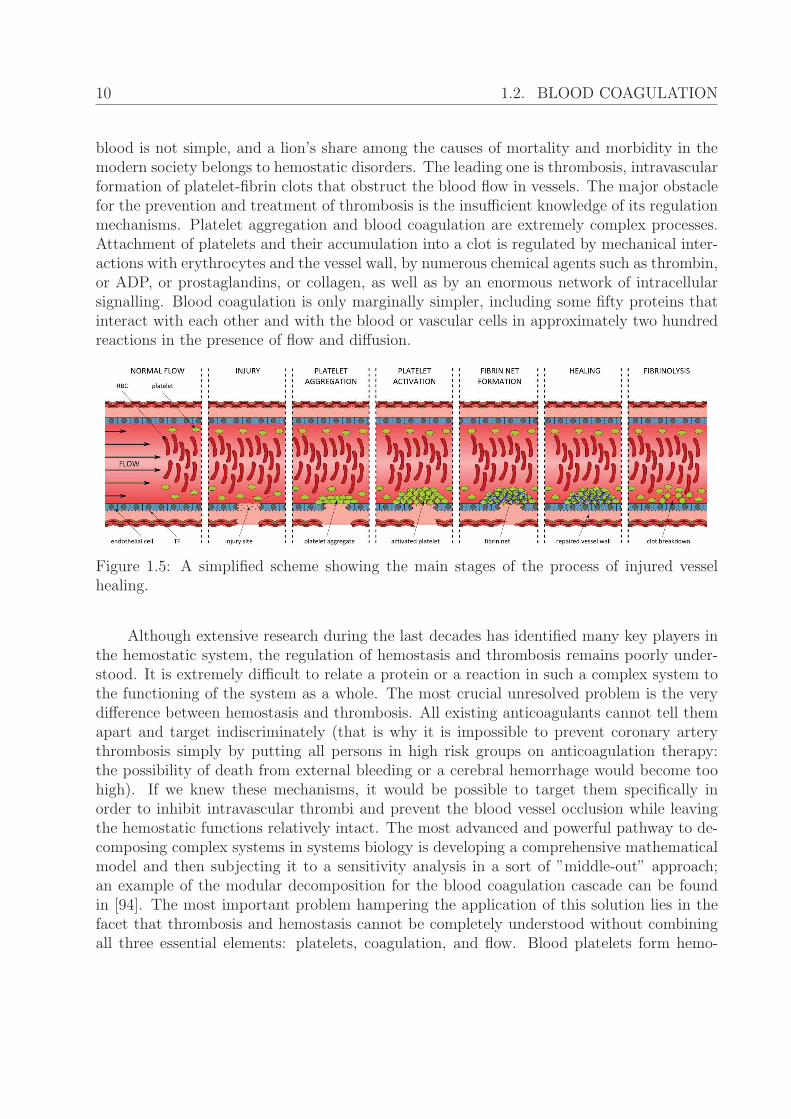
Figure 1.5: A simplified scheme showing the main stages of the process of injured vesselhealing.
Although extensive research during the last decades has identified many key players inthe hemostatic system, the regulation of hemostasis and thrombosis remains poorly under-stood. It is extremely difficult to relate a protein or a reaction in such a complex system tothe functioning of the system as a whole. The most crucial unresolved problem is the verydifference between hemostasis and thrombosis. All existing anticoagulants cannot tell themapart and target indiscriminately (that is why it is impossible to prevent coronary arterythrombosis simply by putting all persons in high risk groups on anticoagulation therapy:the possibility of death from external bleeding or a cerebral hemorrhage would become toohigh). If we knew these mechanisms, it would be possible to target them specifically inorder to inhibit intravascular thrombi and prevent the blood vessel occlusion while leavingthe hemostatic functions relatively intact. The most advanced and powerful pathway to de-composing complex systems in systems biology is developing a comprehensive mathematicalmodel and then subjecting it to a sensitivity analysis in a sort of ”middle-out” approach;an example of the modular decomposition for the blood coagulation cascade can be foundin [94]. The most important problem hampering the application of this solution lies in thefacet that thrombosis and hemostasis cannot be completely understood without combiningall three essential elements: platelets, coagulation, and flow. Blood platelets form hemo-
1.2. BLOOD COAGULATION 11
static plugs and thrombi by aggregation. This process cannot proceed without flow, andis strongly dependent on the platelet-erythrocyte interaction in the presence of flow [112].Blood coagulation is important for the platelet plug formation, because thrombin is one ofthe main activators of platelets ensuring clot/plug stability, and because the fibrin networksolidifies the cell aggregate. In contrast, blood coagulation is strongly inhibited by flow.Active coagulation factors are removed from the site of injury to such a degree that no fibrinclot can be formed at a physiological arterial shear rate [107]. Therefore, the clot formationin the presence of a rapid flow requires platelets that mechanically protect coagulation fromthe flow, provide binding sites for coagulation factors and secrete substances that participatein coagulation such as fibrinogen, factor V, Xi, etc.
One of the most intriguing problems in the field of thrombosis is the problem of reg-ulating the clot size. While the mechanisms of clot growth became well established duringthe last decade [64], it is not clear how and when a clot stops growing in order to avoid acomplete vessel occlusion. One thing that is firmly established is that an occlusion does notalways occur: while the popular experimental model of ferric-chloride induced damage of thecarotid artery usually ends with occlusion [82], there is no occlusion in the laser-induced in-jury model of thrombosis in small arterioles [43]. Numerous hypotheses have been proposedto explain the mechanism by which the clot stops growing (e.g. the role of thrombomodulin[95]). One of the most intriguing ones is the role of fibrin clot - platelet clot interaction: itsuggests the formation of a fibrin cap on the surface of the clot that prevents further theplatelet accumulation [71]. However, the formation of fibrin on the surface of the clot isunlikely because of high shear rates that remove active coagulation factors [107]. In otherwords, the fibrin formation can occur only under the protection of platelets and this preventsthe formation of the fibrin cap on the surface of the platelet clot.
Pathways. Blood coagulation is a complex process involving plasma proteins, called “co-agulation factors”, with the purpose to completely seal the wound. In the case of injury,the blood factors interact in a highly predetermined order, and it is because of this that theblood coagulation regulatory network is sometimes referred to as “the coagulation cascade”.This series of interactions enables the transformation of a blood factor fibrinogen to its poly-merized state called “fibrin polymer”. The purpose of fibrin polymer is to reinforce a plateletaggregate at the injury site, making it more resistant and stronger, thus giving the injuredtissue time to heal. Because of its function and structure the polymerized fibrin reinforcingthe clot is often referred to as “the fibrin net”. The coagulation factors are generally di-vided into two groups – zymogens and cofactors. The zymogens are inactive plasma proteinswhich are, in the presence of other enzymes, transformed to active enzymes. The cofactorsare proteins which act as accelerators or catalysts for other enzymatic reactions. However,some blood factors cannot be classified neither as zymogens nor cofactors. One of theseexceptions is fibrinogen which is transformed to fibrin, which has no enzymatic properties.Coagulation factors are referred to by a system of Roman numerals and when activated aredenoted by the suffix a.
12 1.2. BLOOD COAGULATION
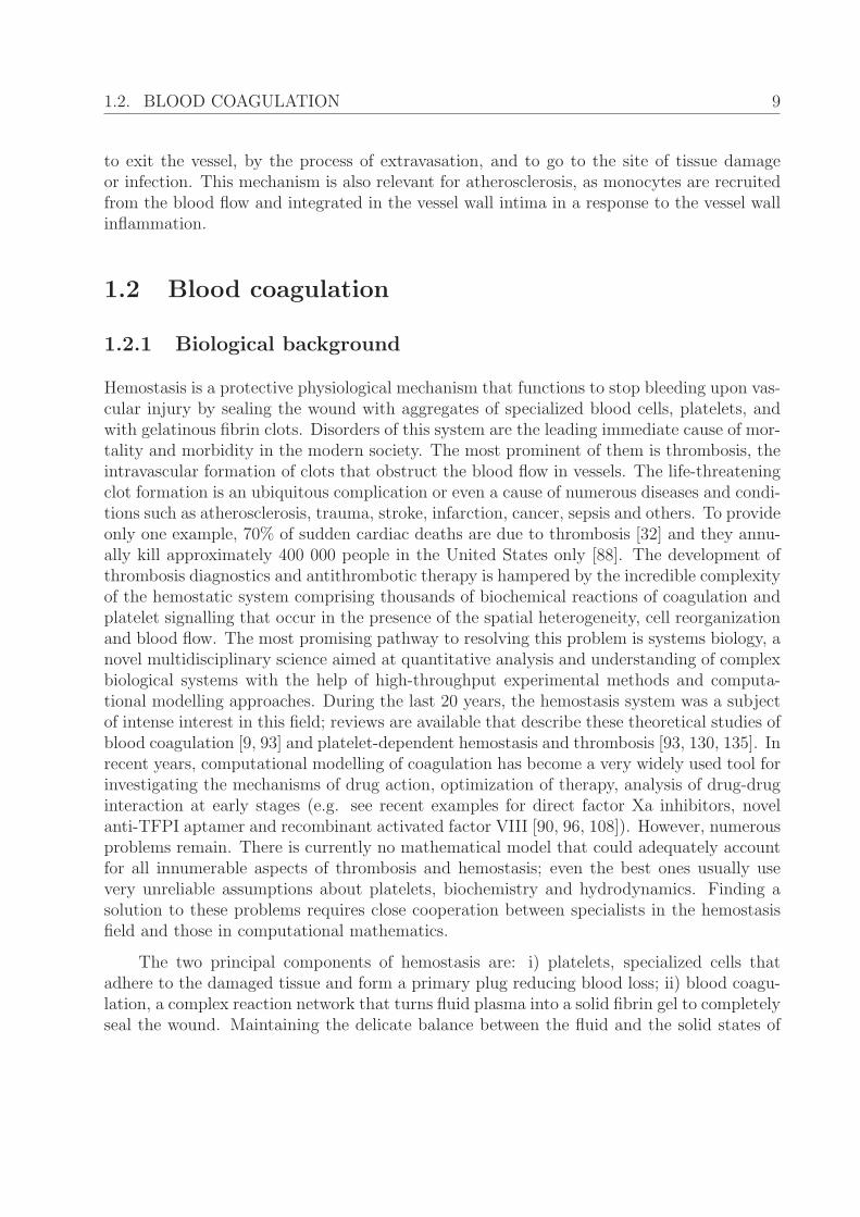
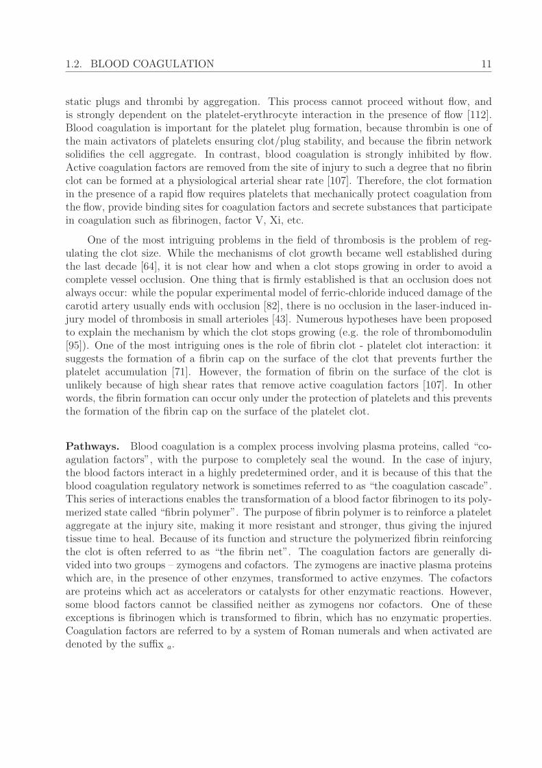
Figure 1.6: Coagulation pathways in vitro - extrinstic, intristic and common. Reprinted withpermission from [92] – C.J. Pallister and M.S. Watson, Scion Publishing Ltd, 2011.
With a view to detecting abnormalities in blood clotting two different in vitro screeningtest were developed: in 1935 A.J. Quick et al described a method based on the prothrom-bin time (PT) [102], while in 1953 R.D. Langdell et al described another screening methodbased on the activated partial thromboplastin time (APTT) [79]. The two methods how-ever yielded different observations about the process of blood coagulation. This led to thedevelopment of two distinct blood coagulation pathways – the extrinsic pathway for PT andthe intrinsic pathway for APTT. Both pathways converge to a so called common pathwayas shown in Figure 1.6. The main difference between the two pathways is in the way theblood coagulation is initiated. The intrinsic pathway is triggered by a contact of flowingblood with a negatively charged surface, such as glass, in which factor XII gets activatedand the intrinsic reaction cascade is started. In the extrinsic pathway the process is initiatedby tissue damage and with the release of tissue factor which forms a complex with bothfactor VII and factor VIIa. These complexes accelerate the activation of factor VII and withit the activation of factor X. In the common pathway, once the factor X gets activated itinduces the production of trombin enzyme from prothrombin. Thrombin then acts as theenzyme in the transformation of fibrinogen to fibrin. As thrombin has multiple enzymaticactivities, including direct activation of factors which are responsible for factor X activa-tion, it also accelerates its own production resulting in an explosive increase in the rate ofcoagulation.
Although the classical model of coagulation pathway, consisting of intrinsic, extrinsicand common pathways, has been very important for understanding the results of laboratoryscreenings, it does not exist as such in vivo. Hence a new model was developed in order to
1.2. BLOOD COAGULATION 13
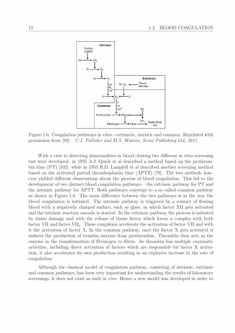
describe blood coagulation in vivo. The model consists of two phases – the initiation phase,followed by the amplification phase. The scheme of each phase is given in Figure 1.7. Themain physiological activator of blood coagulation in vivo is tissue factor. It is expressed onsub-endothelial fibroblasts, injured vascular endothelium and activated monocytes. Hence,in the initiation phase the exposed tissue factor binds with activated factor VIIa to forma complex called “the extrinsic tenase complex”. The complex activates factors IX and Xin a low amount, substantial only for the initiation of a low rate of thrombin production.At this point the level of thrombin is still insufficient to sustain the generation of fibrin ata high rate, and instead it mediates in the activation of factors V and VIII. The formedextrinsic tenase complex is rapidly inactivated by the formation of a complex with factor Xa
and by tissue factor pathway inhibitor (TFPI). In the amplification phase factors IXa andVIIIa bind to form the intrinsic tenase complex. The complex prompts the rapid generationof factor Xa, which is followed by the generation of another complex consisting of factorsXa, Va, calcium ions and platelet phospholipid, called the prothrombinase complex. Theprothrombinase complex induces prothrombin activation to form thrombin. As thrombinacts as the enzyme in the activation of factors V, VIII, XI, it also implicitly accelerates itsown production. The generated thrombin enables the formation of fibrin from fibrinogen.Fibrin monomers are then polymerized in the presence of factor XIIIa, whose production isalso induced by thrombin.
Figure 1.7: Coagulation pathways in vivo - initiation and amplification phase. Reprintedwith permission from [92] – C.J. Pallister and M.S. Watson, Scion Publishing Ltd, 2011.
1.2.2 Modelling
From the modelling point of view, various approaches have been used so far in an attempt tomodel blood coagulation. They can be divided in three main groups - continuous models, dis-crete models and hybrid models. Continuous models rely on a vast mathematical knowledge
14 1.2. BLOOD COAGULATION
of partial differential equations and numerical schemes used to solve them [1, 4, 5, 17, 58, 115].Using PDEs, the hydrodynamic flows can be precisely described, as well as the propagationof blood factors in the blood flow. On the other hand, clot growth depends highly on theblood cells – first of them being platelets as the primary building material of the clot, but alsoon erythrocytes which also strongly influence the blood flow, blood viscosity and the distri-bution of platelets in flow. Due to the more discrete nature of the clot formation, continuousmodels were unable to capture cell interactions and processes like the rupture of a clot. Indiscrete approaches the most of the used methods consider the simulated medium to consistof particles, usually representing atoms, molecules, small lumps of the medium or cells. Thisallows the description of a heterogeneous medium while keeping the ability to approximateits hydrodynamic properties in the flow [99, 119]. The difficulty arises with the modellingof the complex regulatory network of proteins involved in coagulation and their transport inthe flow. Here comes the idea of developing hybrid models which would use both continuousand discrete methods with the intention of coupling their strengths and avoiding as muchas possible their downfalls. Among the hybrid models various approaches have been used,each of them taking their own ratio of continuous and discrete parts. A number of hybridmethods use the continuous concept to model blood flow and propagation of blood factors init, while the discrete concept is used to model blood cells and interactions between them. In[51, 98, 111, 131, 132, 133, 134] the blood flow is described by Navier-Stokes equations. Themotion of blood cells in the blood flow then follows from the calculated velocity field. As theflow simulation domain changes because of the clot development, the Immersed Boundary(IB) method is often used. The protein cascade is described with a system of differentialequations, each equation describing a concentration of a single blood factor. Blood cells andtheir interactions are modelled with a discrete method like Cellular Potts Method (CPM)[131, 132, 133, 134] or with the method of Subcellular Elements (SCE) [111]. Another hybridapproach is to model the blood flow (blood plasma and blood cells) with a discrete methodand to model the regulatory network of blood factors by a system of PDEs. One of the earlyworks applying this method is [49].
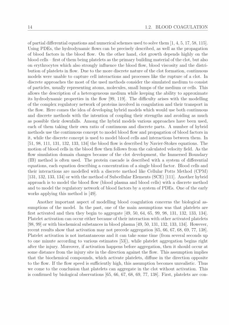
Another important aspect of modelling blood coagulation concerns the biological as-sumptions of the model. In the past, one of the main assumptions was that platelets arefirst activated and then they begin to aggregate [49, 50, 64, 65, 99, 98, 131, 132, 133, 134].Platelet activation can occur either because of their interaction with other activated platelets[98, 99] or with biochemical substances in blood plasma [49, 50, 131, 132, 133, 134]. However,recent results show that activation may not precede aggregation [65, 66, 67, 68, 69, 77, 138].Platelet activation is not instantaneous and it can take some time (from several seconds upto one minute according to various estimates [53]), while platelet aggregation begins rightafter the injury. Moreover, if activation happens before aggregation, then it should occur atsome distance from the injury site in the direction against the flow. This assumption impliesthat the biochemical compounds, which activate platelets, diffuse in the direction oppositeto the flow. If the flow speed is sufficiently high, this assumption becomes unrealistic. Thuswe come to the conclusion that platelets can aggregate in the clot without activation. Thisis confirmed by biological observations [65, 66, 67, 68, 69, 77, 138]. First, platelets are con-
1.3. ATHEROSCLEROSIS 15
nected by weak reversible bonds due to GPIb receptors. A new platelet coming from the flowcan roll at the surface of the clot, slowing down because of these weak reversible connections.When it stops, other receptors (integrin) create more stable connections due to platelet ac-tivation. Finally, platelets can be covered by fibrin net, which fixes them completely in theclot. Thus we consider another concept of clot growth where platelet activation does not pre-cede platelet aggregation but, on the contrary, follows the first stage of clot formation. Oneof the main objectives of this work is to test this hypothesis in numerical simulations.
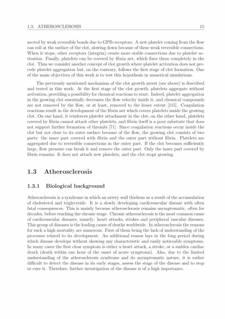
The previously mentioned mechanism of the clot growth arrest (see above) is describedand tested in this work. At the first stage of the clot growth, platelets aggregate withoutactivation, providing a possibility for chemical reactions to start. Indeed, platelet aggregationin the growing clot essentially decreases the flow velocity inside it, and chemical compoundsare not removed by the flow, or at least, removed to the lesser extent [115]. Coagulationreactions result in the development of the fibrin net which covers platelets inside the growingclot. On one hand, it reinforces platelet attachment in the clot, on the other hand, plateletscovered by fibrin cannot attach other platelets, and fibrin itself is a poor substrate that doesnot support further formation of thrombi [71]. Since coagulation reactions occur inside theclot but not close to its outer surface because of the flow, the growing clot consists of twoparts: the inner part covered with fibrin and the outer part without fibrin. Platelets areaggregated due to reversible connections in the outer part. If the clot becomes sufficientlylarge, flow pressure can break it and remove the outer part. Only the inner part covered byfibrin remains. It does not attach new platelets, and the clot stops growing.
1.3 Atherosclerosis
1.3.1 Biological background
Atherosclerosis is a syndrome in which an artery wall thickens as a result of the accumulationof cholesterol and triglyceride. It is a slowly developing cardiovascular disease with oftenfatal consequences. This is mainly because atherosclerosis remains asymptomatic, often fordecades, before reaching the chronic stage. Chronic atherosclerosis is the most common causeof cardiovascular diseases, namely: heart attacks, strokes and peripheral vascular diseases.This group of diseases is the leading cause of deaths worldwide. In atherosclerosis the reasonsfor such a high mortality are numerous. First of them being the lack of understanding of theprocesses related to its development. An additional reason lays in the long period duringwhich disease develops without showing any characteristic and easily noticeable symptoms.In many cases the first clear symptom is either a heart attack, a stroke, or a sudden cardiacdeath (death within one hour of the onset of acute symptoms). Also, due to the limitedunderstanding of the atherosclerosis syndrome and its asymptomatic nature, it is ratherdifficult to detect the disease in its early stages, assess the stage of the disease and to stopor cure it. Therefore, further investigation of the disease is of a high importance.
16 1.3. ATHEROSCLEROSIS
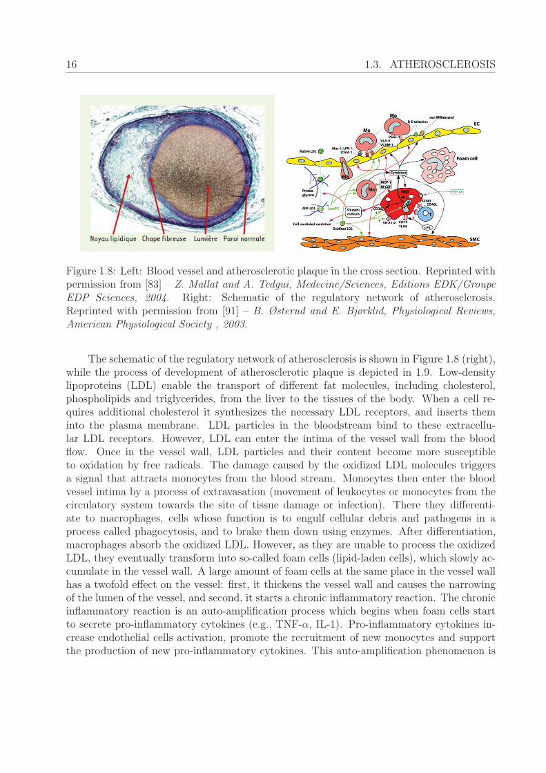
Figure 1.8: Left: Blood vessel and atherosclerotic plaque in the cross section. Reprinted withpermission from [83] – Z. Mallat and A. Tedgui, Medecine/Sciences, Editions EDK/GroupeEDP Sciences, 2004. Right: Schematic of the regulatory network of atherosclerosis.Reprinted with permission from [91] – B. Østerud and E. Bjørklid, Physiological Reviews,American Physiological Society , 2003.
The schematic of the regulatory network of atherosclerosis is shown in Figure 1.8 (right),while the process of development of atherosclerotic plaque is depicted in 1.9. Low-densitylipoproteins (LDL) enable the transport of different fat molecules, including cholesterol,phospholipids and triglycerides, from the liver to the tissues of the body. When a cell re-quires additional cholesterol it synthesizes the necessary LDL receptors, and inserts theminto the plasma membrane. LDL particles in the bloodstream bind to these extracellu-lar LDL receptors. However, LDL can enter the intima of the vessel wall from the bloodflow. Once in the vessel wall, LDL particles and their content become more susceptibleto oxidation by free radicals. The damage caused by the oxidized LDL molecules triggersa signal that attracts monocytes from the blood stream. Monocytes then enter the bloodvessel intima by a process of extravasation (movement of leukocytes or monocytes from thecirculatory system towards the site of tissue damage or infection). There they differenti-ate to macrophages, cells whose function is to engulf cellular debris and pathogens in aprocess called phagocytosis, and to brake them down using enzymes. After differentiation,macrophages absorb the oxidized LDL. However, as they are unable to process the oxidizedLDL, they eventually transform into so-called foam cells (lipid-laden cells), which slowly ac-cumulate in the vessel wall. A large amount of foam cells at the same place in the vessel wallhas a twofold effect on the vessel: first, it thickens the vessel wall and causes the narrowingof the lumen of the vessel, and second, it starts a chronic inflammatory reaction. The chronicinflammatory reaction is an auto-amplification process which begins when foam cells startto secrete pro-inflammatory cytokines (e.g., TNF-α, IL-1). Pro-inflammatory cytokines in-crease endothelial cells activation, promote the recruitment of new monocytes and supportthe production of new pro-inflammatory cytokines. This auto-amplification phenomenon is
1.3. ATHEROSCLEROSIS 17
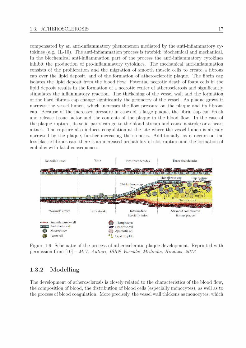
compensated by an anti-inflammatory phenomenon mediated by the anti-inflammatory cy-tokines (e.g., IL-10). The anti-inflammation process is twofold: biochemical and mechanical.In the biochemical anti-inflammation part of the process the anti-inflammatory cytokinesinhibit the production of pro-inflammatory cytokines. The mechanical anti-inflammationconsists of the proliferation and the migration of smooth muscle cells to create a fibrouscap over the lipid deposit, and of the formation of atherosclerotic plaque. The fibrin capisolates the lipid deposit from the blood flow. Potential necrotic death of foam cells in thelipid deposit results in the formation of a necrotic center of atherosclerosis and significantlystimulates the inflammatory reaction. The thickening of the vessel wall and the formationof the hard fibrous cap change significantly the geometry of the vessel. As plaque grows itnarrows the vessel lumen, which increases the flow pressure on the plaque and its fibrouscap. Because of the increased pressure in cases of a large plaque, the fibrin cap can breakand release tissue factor and the contents of the plaque in the blood flow. In the case ofthe plaque rupture, its solid parts can go to the blood stream and cause a stroke or a heartattack. The rupture also induces coagulation at the site where the vessel lumen is alreadynarrowed by the plaque, further increasing the stenosis. Additionally, as it occurs on theless elastic fibrous cap, there is an increased probability of clot rupture and the formation ofembolus with fatal consequences.
Figure 1.9: Schematic of the process of atherosclerotic plaque development. Reprinted withpermission from [10] – M.V. Autieri, ISRN Vascular Medicine, Hindawi, 2012.
1.3.2 Modelling
The development of atherosclerosis is closely related to the characteristics of the blood flow,the composition of blood, the distribution of blood cells (especially monocytes), as well as tothe process of blood coagulation. More precisely, the vessel wall thickens as monocytes, which
18 1.3. ATHEROSCLEROSIS
roll on the inner surface of the vessel, enter the vessel wall intima in a response to the badcholesterol accumulation. Furthermore, at a chronic stage of atherosclerosis the thickeningof the vessel wall can be severe and result in a remodelling of the vessel and significantchanges in the flow configuration at the inflammation site. Due to the vessel remodellingthe stress from the flow on the vessel wall at the inflammation site can significantly increase,leading to a rupture of the thrombotic plaque. The parts of the ruptured plaque can leadto a stroke or a heart attack. Additionally, the blood coagulation process will begin and aclot will form at the inflammation site, increasing further the stenosis of the vessel. In thiscase, the otherwise normal coagulation process can be compromised by the altered vesselwall properties (plaque) and stenosis, possibly leading to further complications such as clotrupture or vascular occlusion. Because of this the modelling of atherosclerosis is closelyrelated to modelling of the blood flow, blood cells, and blood coagulation.
Another aspect of studying the development of atherosclerosis is related to chronic in-flammation. The theory of atherosclerosis as an inflammatory disease is well accepted [35],although the process is not yet completely understood and other theories have also been de-veloped in the last decades. The inflammatory aspect of atherosclerosis makes it suitable formodelling and studying with partial differential equations. This approach allows to describethe inflammation propagation as a wave solution of a parabolic partial differential equation.Depending on the initial conditions, the system can stay in the disease free equilibrium,or a travelling wave propagation can occur, which corresponds to a chronic inflammatoryresponse.
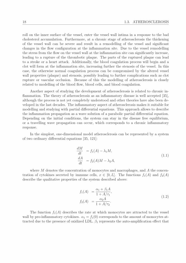
In the simplest, one-dimensional model atherosclerosis can be represented by a systemof two ordinary differential equations [35, 121]:
dM
dt= f1(A)− λ1M,
dA
dt= f2(A)M − λ2A,
(1.1)
where M denotes the concentration of monocytes and macrophages, and A the concen-tration of cytokines secreted by immune cells, x ∈ [0, L]. The functions f1(A) and f2(A)describe the qualitative properties of the system described above:
f1(A) =α1 + β1A
1 + A/τ1,
f2(A) =α2A
1 + A/τ2.
(1.2)
The function f1(A) describes the rate at which monocytes are attracted to the vesselwall by pro-inflammatory cytokines. α1 = f1(0) corresponds to the amount of monocytes at-tracted due to the presence of oxidized LDL. β1 represents the auto-amplification effect that
1.3. ATHEROSCLEROSIS 19
occurs as monocytes secrete more pro-inflammatory cytokines that attract even more mono-cytes to the inflammation site. The factor 1+A/τ1 represents the mechanical obstruction ofthe recruitment of new monocytes due to the formation of a fibrous cap, where τ1 denotesthe characteristic time of the fibrous cap formation. Term f2(A)M modells the cytokineproduction rate, where α2A describes the auto-promoted secretion of pro-inflammatory cy-tokines, and 1+A/τ2 describes the inhibition of the pro-inflammatory cytokine secretion byanti-inflammatory cytokines. Here τ2 represents the time that is necessary for the inhibitionto commence. λ1 and λ2 denote the degradation rates of immune cells and cytokines respec-tively, while d1 and d2 describe the corresponding diffusion (or cell displacement) rates inthe vessel intima.
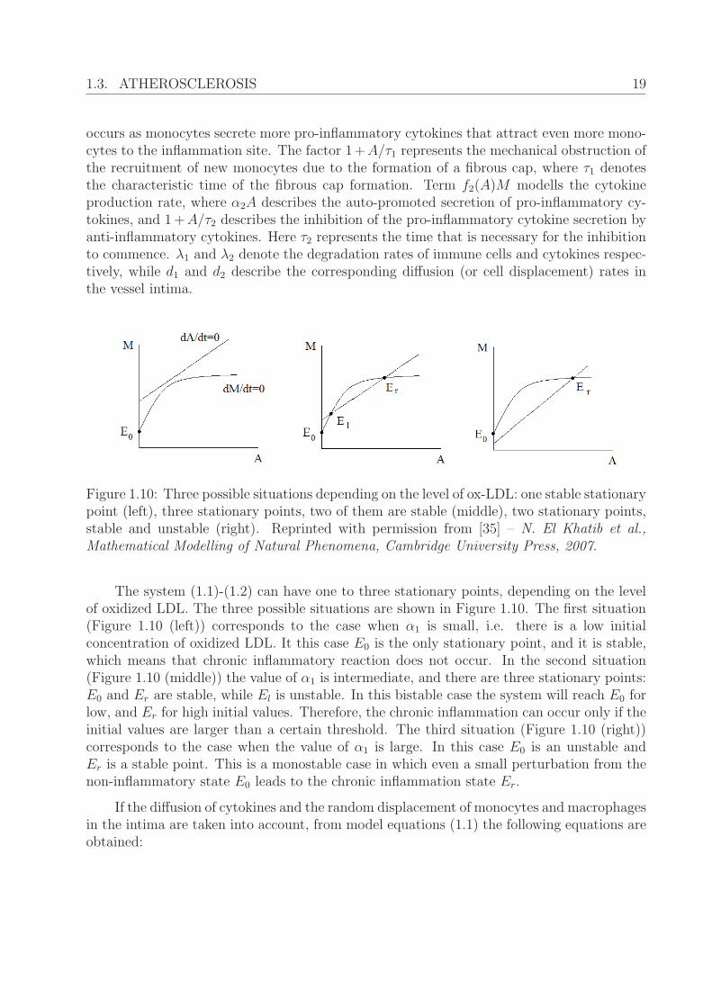
Figure 1.10: Three possible situations depending on the level of ox-LDL: one stable stationarypoint (left), three stationary points, two of them are stable (middle), two stationary points,stable and unstable (right). Reprinted with permission from [35] – N. El Khatib et al.,Mathematical Modelling of Natural Phenomena, Cambridge University Press, 2007.
The system (1.1)-(1.2) can have one to three stationary points, depending on the levelof oxidized LDL. The three possible situations are shown in Figure 1.10. The first situation(Figure 1.10 (left)) corresponds to the case when α1 is small, i.e. there is a low initialconcentration of oxidized LDL. It this case E0 is the only stationary point, and it is stable,which means that chronic inflammatory reaction does not occur. In the second situation(Figure 1.10 (middle)) the value of α1 is intermediate, and there are three stationary points:E0 and Er are stable, while El is unstable. In this bistable case the system will reach E0 forlow, and Er for high initial values. Therefore, the chronic inflammation can occur only if theinitial values are larger than a certain threshold. The third situation (Figure 1.10 (right))corresponds to the case when the value of α1 is large. In this case E0 is an unstable andEr is a stable point. This is a monostable case in which even a small perturbation from thenon-inflammatory state E0 leads to the chronic inflammation state Er.
If the diffusion of cytokines and the random displacement of monocytes and macrophagesin the intima are taken into account, from model equations (1.1) the following equations areobtained:
20 1.3. ATHEROSCLEROSIS
∂M
∂t= d1
∂2M
∂x2+ f1(A)− λ1M,
∂A
∂t= d2
∂2A
∂x2+ f2(A)M − λ2A,
(1.3)
where d1 is the cell displacement coefficient, d2 is the cytokine diffusion coefficient, andthe definition of functions f1(A) remains unchanged f2(A) (equations (1.2)). The existence ofthe travelling wave solution for the reaction diffusion system (1.2)-(1.3) is proven in [35].
Although, the inflammatory reaction in atherosclerosis occurs in the vessel intima, theone-dimensional model (equations (1.2) and (1.3)) does not take into account the processof extravasation, by which monocytes from the blood flow enter the vessel intima. Hence,a two-dimensional model was proposed in [36, 37, 38], where the recruitment of monocytesis described in terms of a boundary condition. The domain of the model is an infinite stripΩ = {(x, y) : −∞ < x < ∞, 0 ≤ y ≤ h} which represents again the vessel intima, where hdenotes its thickness. The model is then described by the following system of equations:
∂M
∂t= dMΔM + βM,
∂A
∂t= dAΔA+ f(A)M − γA+ bs.
(1.4)
with the corresponding boundary conditions:
y = 0 :∂M
∂y= 0,
∂A
∂y= 0,
y = h :∂M
∂y= g(A),
∂A
∂y= 0.
(1.5)
The boundary conditions at y = 0 are homogeneous Neumann as they describe thecondition with no flux of monocytes and cytokines through the boundary. At y = h theflux of monocytes is non-zero and depends on the level of cytokines, while there is againno flux of cytokines. The system (1.4)-(1.5) is a reaction-diffusion system in an unboundeddomain with non-linear boundary conditions. As such the classical results for semi-linearparabolic problems (Volpert et al. 2000) [122] are not applicable to this problem. Therefore,in [37, 38] the existence of a travelling wave is proven in the monostable case. Additionally, itis numerically shown [37, 38] that as h goes to zero, the solution of the 2D problem convergesto the solution of the above mentioned 1D problem [35].
1.4. MAIN RESULTS OF THE THESIS 21
1.4 Main results of the thesis
The main subject of this thesis is the modelling of blood flow related phenomena by usinghybrid models. More precisely, a mathematical hybrid model is developed to study thebiological process of blood coagulation. The second chapter contains the description of adiscrete method, called Dissipative Particle Dynamics (DPD), which is a particle methodused to model the flow of blood plasma. The description of the method is followed by adescription of integration schemes for equations of motions, containing a novel integrationscheme for DPD, which allows a significant increase of the time step for DPD. In Section 2.2methods of measuring physical properties in simulations are explained. As in DPD methodmodelling of boundaries can pose a problem, Section 2.3 contains descriptions of multipleways to implement no-slip boundary conditions in DPD. The final section of the first chapter(Section 2.4) discusses the modelling of the erythrocyte membrane in DPD for both 2D and3D case.
The third and fourth chapter concern the modelling of blood coagulation in flow. In theChapter 3 a discrete model of clot growth in flow is described. In the model, blood plasmaand platelets are modelled by the DPD method, while the platelet aggregation is modelledby Hooke’s law. The model is used to study several approaches to modelling different inter-platelet bonds. Furthermore, it is used for a preliminary study of a possible mechanism ofgrowth arrest of the platelet clot, which will be further studied in hybrid models. Chapter4 describes two hybrid (discrete-continuous) models. Section 4.1 describes the first hybridmodel. The discrete part of the model uses DPD to describe platelets suspended in theplasma flow, while the continuous part consists of a single reaction-diffusion-advection equa-tion which describes the concentration of fibrin. The model is used to calibrate parametersand methods used to combine the discrete and the continuous parts of the model, as wellas to study the interaction between the platelet aggregate and a blood factor concentrationin flow. In Section 4.2 the second hybrid model is described. Instead of the single reaction-diffusion-advection equation, the blood coagulation pathways are modelled by a system ofthree equations. The system simulates the main characteristics of the coagulation cascade:the self-accelerated thrombin production from prothrombin, the influence of thrombin con-centration on the transformation of fibrinogen to fibrin, and the influence of the flow onconcentrations of blood factors. The model is used to study the influence of the platelet clotformation on the blood factor concentrations in flow. It showed the importance of the inter-action between the platelet aggregation and coagulation pathways. Since the flow velocityis small inside the platelet clot, it is possible for the coagulation cascade to begin and toreinforce the growing aggregate by the formation of a fibrin network. The pressure from theblood flow removes the outer parts of the platelet clot and eventually stops it growth sincethe platelets covered by fibrin cannot attach new platelets [71]. Thus we suggest a possiblemechanism how platelet clot stops growing. It is different from the mechanism which stopsthe coagulation cascade in blood plasma, though they interact with each other. The end ofSection 4.2 contains simulation results of clot growth in vessels of different diameters and in
22 1.4. MAIN RESULTS OF THE THESIS
flows of different wall shear rates, obtained by use of the second hybrid model.
The fifth chapter is devoted to the mathematical analysis of a model of chronic inflam-mation related to atherosclerosis. Previously it was shown that the inflammation propagatesas a reaction-diffusion wave whose properties depend on the level of the bad cholesterol inblood [38]. In this thesis we study a model problem which describes the propagation ofa reaction-diffusion wave in the 2D case with nonlinear boundary conditions. The Leray-Schauder method and a priori estimates of solutions are used in order to prove the existenceof waves in the bistable case.
The thesis concludes with a section containing all the relevant references used in thiswork, and the Appendix section containing a description of the numerical implementationof the models developed in this work. These details are gathered to the independent sectionin order to separate them from model descriptions and results, and to make the structureof the thesis easier to follow. However, the models of blood flows that describe blood as aplasma suspension of blood cells, as well as the blood coagulation models developed in thiswork, are computationally very expensive. Hence, in the scope of the work described in thethesis a substantial effort was directed to optimization and parallelization of the numericalimplementation.
23
Chapter 2
Dissipative Particle Dynamics
2.1 Description
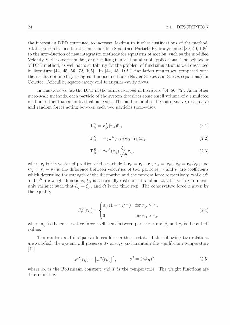
In order to simulate a complex fluid, a numerical method has to describe the structure of thefluid, usually on the microscopic level, for which classical continuous and discrete methodsare not suitable. Continuous approaches, like Navier-Stokes equations, although useful formodelling simple fluids, lack the ability to model the composite structure of complex fluids.On the other hand, Molecular Dynamics (MD) as a classical discrete approach, althoughable to capture the complex structure of the fluid, is inappropriate because it becomes tooexpensive to study macroscopic phenomena on a larger scale. Hence, so-called meso-scalemethods were developed. In order to describe a certain complex structure on a micro-scaleand to still be able to study its effects on a macro-scale the meso-scale methods use “coarse-graining” - the process of representing a system with fewer degrees of freedom than thoseactually present in the system [41, 105]. Many of such methods are not strictly mathemat-ically derived but are rather constructed in order to satisfy certain conservation laws andsymmetries that are considered to be essential for the observed phenomena. Since the in-terest in this area began thirty years ago, a lot of meso-scale methods and their specialisedvariants were developed and a lot of effort was done in order to succumb their potentialflaws, as well as to justify their definition by deriving them from continuous methods andconservation laws. One of the most successful and generally used methods is DissipativeParticle Dynamics (DPD) which was first described by Hoogerbrugge and Koelman in 1992[61, 105]. By its definition DPD is a mass and momentum conservative method, and itproduces a correct hydrodynamic behaviour, which was verified both analytically and bysimulations. In its original description the DPD method does not conserve the energy of thesystem, due to its definition of dissipative and random forces. However, a rigorous theoreti-cal justification was later given by Espanol and Warren who derived the correct fluctuationdissipation relation for the friction and noise terms in 1995. In the same year, Espanol de-rived the hydrodynamic equations for the mass and momentum density fields. Since then
24 2.1. DESCRIPTION
the interest in DPD continued to increase, leading to further justifications of the method,establishing relations to other methods like Smoothed Particle Hydrodynamics [39, 40, 105],to the introduction of new integration methods for equations of motion, such as the modifiedVelocity-Verlet algorithm [56], and resulting in a vast number of applications. The behaviourof DPD method, as well as its suitability for the problem of fluid simulation is well describedin literature [44, 45, 56, 72, 105]. In [44, 45] DPD simulation results are compared withthe results obtained by using continuous methods (Navier-Stokes and Stokes equations) forCouette, Poiseuille, square-cavity and triangular-cavity flows.
In this work we use the DPD in the form described in literature [44, 56, 72]. As in othermeso-scale methods, each particle of the system describes some small volume of a simulatedmedium rather than an individual molecule. The method implies the conservative, dissipativeand random forces acting between each two particles (pair-wise):
FCij = FC
ij (rij)rij, (2.1)
FDij = −γωD(rij)(vij · rij)rij, (2.2)
FRij = σωR(rij)
ξij√dtrij, (2.3)
where ri is the vector of position of the particle i, rij = ri − rj, rij = |rij|, rij = rij/rij, andvij = vi − vj is the difference between velocities of two particles, γ and σ are coefficientswhich determine the strength of the dissipative and the random force respectively, while ωD
and ωR are weight functions; ξij is a normally distributed random variable with zero mean,unit variance such that ξij = ξji, and dt is the time step. The conservative force is given bythe equality
FCij (rij) =
⎧⎨⎩aij (1− rij/rc) for rij ≤ rc,
0 for rij > rc,(2.4)
where aij is the conservative force coefficient between particles i and j, and rc is the cut-offradius.
The random and dissipative forces form a thermostat. If the following two relationsare satisfied, the system will preserve its energy and maintain the equilibrium temperature[42]
ωD(rij) =[ωR(rij)
]2, σ2 = 2γkBT, (2.5)
where kB is the Boltzmann constant and T is the temperature. The weight functions aredetermined by:
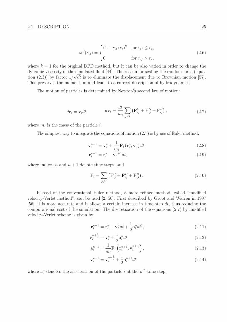
2.1. DESCRIPTION 25
ωR(rij) =
⎧⎨⎩(1− rij/rc)k for rij ≤ rc,
0 for rij > rc,(2.6)
where k = 1 for the original DPD method, but it can be also varied in order to change thedynamic viscosity of the simulated fluid [44]. The reason for scaling the random force (equa-tion (2.3)) by factor 1/
√dt is to eliminate the displacement due to Brownian motion [57].
This preserves the momentum and leads to a correct description of hydrodynamics.
The motion of particles is determined by Newton’s second law of motion:
dri = vidt, dvi =dt
mi
∑j �=i
(FCij + FD
ij + FRij
), (2.7)
where mi is the mass of the particle i.
The simplest way to integrate the equations of motion (2.7) is by use of Euler method:
vn+1i = vni +
1
mi
Fi (rni ,v
ni ) dt, (2.8)
rn+1i = rni + vn+1
i dt, (2.9)
where indices n and n+ 1 denote time steps, and
Fi =∑j �=i
(FCij + FD
ij + FRij
). (2.10)
Instead of the conventional Euler method, a more refined method, called “modifiedvelocity-Verlet method”, can be used [2, 56]. First described by Groot and Warren in 1997[56], it is more accurate and it allows a certain increase in time step dt, thus reducing thecomputational cost of the simulation. The discretization of the equations (2.7) by modifiedvelocity-Verlet scheme is given by:
rn+1i = rni + vni dt+
1
2ani dt
2, (2.11)
vn+ 1
2i = vni +
1
2ani dt, (2.12)
an+1i =
1
mi
Fi
(rn+1i ,v
n+ 12
i
), (2.13)
vn+1i = v
n+ 12
i +1
2an+1i dt, (2.14)
where ani denotes the acceleration of the particle i at the nth time step.
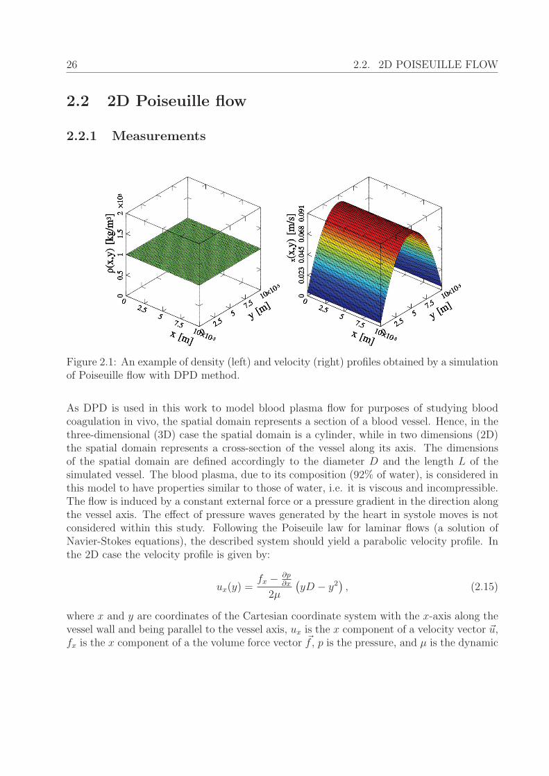
26 2.2. 2D POISEUILLE FLOW
2.2 2D Poiseuille flow
2.2.1 Measurements
Figure 2.1: An example of density (left) and velocity (right) profiles obtained by a simulationof Poiseuille flow with DPD method.
As DPD is used in this work to model blood plasma flow for purposes of studying bloodcoagulation in vivo, the spatial domain represents a section of a blood vessel. Hence, in thethree-dimensional (3D) case the spatial domain is a cylinder, while in two dimensions (2D)the spatial domain represents a cross-section of the vessel along its axis. The dimensionsof the spatial domain are defined accordingly to the diameter D and the length L of thesimulated vessel. The blood plasma, due to its composition (92% of water), is considered inthis model to have properties similar to those of water, i.e. it is viscous and incompressible.The flow is induced by a constant external force or a pressure gradient in the direction alongthe vessel axis. The effect of pressure waves generated by the heart in systole moves is notconsidered within this study. Following the Poiseuile law for laminar flows (a solution ofNavier-Stokes equations), the described system should yield a parabolic velocity profile. Inthe 2D case the velocity profile is given by:
ux(y) =fx − ∂p
∂x
2μ
(yD − y2
), (2.15)
where x and y are coordinates of the Cartesian coordinate system with the x-axis along thevessel wall and being parallel to the vessel axis, ux is the x component of a velocity vector �u,fx is the x component of a the volume force vector �f , p is the pressure, and μ is the dynamic
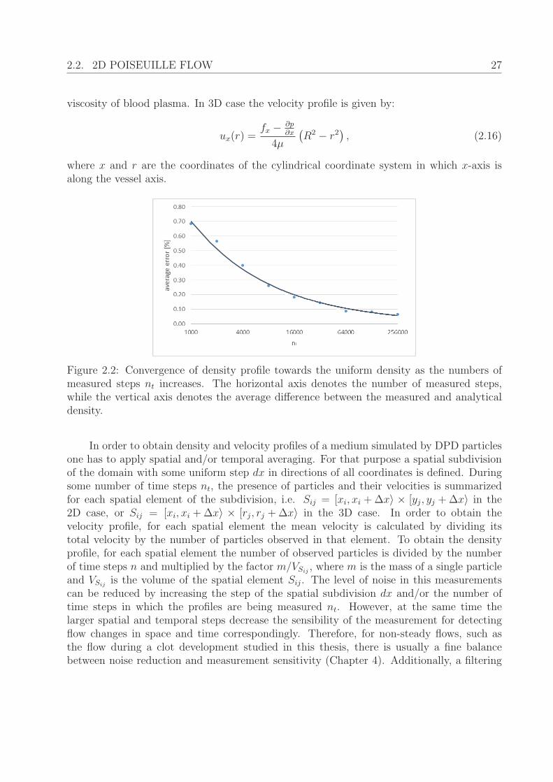
2.2. 2D POISEUILLE FLOW 27
viscosity of blood plasma. In 3D case the velocity profile is given by:
ux(r) =fx − ∂p
∂x
4μ
(R2 − r2
), (2.16)
where x and r are the coordinates of the cylindrical coordinate system in which x-axis isalong the vessel axis.
Figure 2.2: Convergence of density profile towards the uniform density as the numbers ofmeasured steps nt increases. The horizontal axis denotes the number of measured steps,while the vertical axis denotes the average difference between the measured and analyticaldensity.
In order to obtain density and velocity profiles of a medium simulated by DPD particlesone has to apply spatial and/or temporal averaging. For that purpose a spatial subdivisionof the domain with some uniform step dx in directions of all coordinates is defined. Duringsome number of time steps nt, the presence of particles and their velocities is summarizedfor each spatial element of the subdivision, i.e. Sij = [xi, xi +Δx〉 × [yj, yj +Δx〉 in the2D case, or Sij = [xi, xi +Δx〉 × [rj, rj +Δx〉 in the 3D case. In order to obtain thevelocity profile, for each spatial element the mean velocity is calculated by dividing itstotal velocity by the number of particles observed in that element. To obtain the densityprofile, for each spatial element the number of observed particles is divided by the numberof time steps n and multiplied by the factor m/VSij
, where m is the mass of a single particleand VSij
is the volume of the spatial element Sij. The level of noise in this measurementscan be reduced by increasing the step of the spatial subdivision dx and/or the number oftime steps in which the profiles are being measured nt. However, at the same time thelarger spatial and temporal steps decrease the sensibility of the measurement for detectingflow changes in space and time correspondingly. Therefore, for non-steady flows, such asthe flow during a clot development studied in this thesis, there is usually a fine balancebetween noise reduction and measurement sensitivity (Chapter 4). Additionally, a filtering
28 2.2. 2D POISEUILLE FLOW
or smoothing methods can be used to reduce the noise. Due to the suitability of the DPDmethod for modelling hydrodynamics, with properly defined boundary conditions the densityand velocity profiles will converge to the corresponding analytical solution of Navier-Stokesequations as nt increases. An example of the smooth density and velocity profiles obtainedby DPD method for the case of Poiseuille flow is shown in the Figure 2.1.
2.2.2 Physical parameters in 2D
In a 2D DPD simulation some physical values, like the particle volume and mass, have tobe reinterpreted. Let us consider the simulation of a homogeneous fluid (like water or bloodplasma), where all DPD particles in the system can be considered to have the same properties(mass, volume, inter-particle DPD forces). Then the 2D problem can be interpreted as alayer of DPD particles whose movement is restricted to a single plane. This enables the 3Dinterpretation of all parameters and the calculation of corresponding physical properties. Asa result, in the 2D method physical parameters can be directly defined and used. Thus, ina 2D DPD simulation, next to the DPD parameters, the following physical parameters arenecessary and sufficient to determine flow properties in the vessel: vessel diameter D andlength L, density ρ, viscosity μ, mean flow velocity ux and only one discretization parameterNy, representing the number of particles in the y cross-section in their initial positions (onthe regular grid with a uniform step). From the values of these parameters the values of theremaining parameters can be deduced - the mass and the volume of a single particle, as wellas the body force necessary to induce the flow. Because of the uniform step of the grid forthe initial positions of particles we can write:
L
Nx
=D
Ny
=H
Nz
, (2.17)
where H is the thickness (3rd dimension) of the volume defined by the layer of particles inthe simulated plane, while Nx and Nz are defined analogously to Ny. Note that Nz is equalto 1, as the particles are contained in a plane. Then the values of Nx and H can be directlyobtained from the equation (2.17). The volume V of the particle layer can be on the onehand expressed as the product of its dimensions, and on the other as the sum of volumes ofall particles. Thus we have:
LDH = V = NxNyNzVp, (2.18)
where Vp is the volume of a single particle. It follows that the particle volume is equal toH3. Finally, the mass of a single particle is given by m = ρVp. The value of volume force fxcan be obtained from the equation (2.15), and the corresponding acceleration G is given bydividing the volume force by density, G = fx/ρ.
2.2. 2D POISEUILLE FLOW 29
2.2.3 Calculating viscosity
Although the values of the physical parameters of a simulated fluid can be set a priori,the values of DPD parameters have to be determined experimentally in order to obtain thewanted value of viscosity. The calibration of DPD parameters, σ, γ, aij, rc and k, canbe done by simulating a Poiseuille flow and comparing it to the corresponding solution ofNavier-Stokes equations [11]. By integrating the equation (2.15) and dividing it by the vesseldiameter, one obtains the expression for the average flow velocity in the 2D case as a functionof the dynamic viscosity, the channel diameter and the external force (or pressure):
ux =
(fx − ∂p
∂x
)D2
12μ. (2.19)
where ux is the average flow velocity in the direction tangential to the vessel axis. By analogythe average flow velocity in the 3D case is given by:
ux =
(fx − ∂p
∂x
)R2
8μ, (2.20)
Therefore, for the given DPD parameters, physical parameters and the volume force, theaverage flow velocity can be measured in a simulation and the viscosity of the simulated fluidcan be calculated. The influence of the DPD parameters on the viscosity of the simulatedfluid is shown in the Figure 2.4. The cut-off radius has a great impact on the viscosity ofthe fluid, however, it has an even greater impact on the computational cost. Hence, it isbetter to keep it as low as possible, and, if necessary, to increase the viscosity via otherDPD parameters. Among the strength coefficients of the three DPD forces, σ, γ and aij,the dissipative force coefficient σ has the largest influence on the viscosity of the simulatedfluid. The conservative force coefficient aij regulates the compressibility of the simulatedfluid. While it also has a mild influence on the viscosity, by increasing it too much thevelocity profile ceases to be parabolic (Figure 2.3). This effect can be counteracted by thesimultaneous increase of the value of the random force coefficient γ, as it brings more energyto the system and enables particles to move more easily. Increasing values of any of thethree force coefficients can result in a decrease of the upper limit of the time step, thusincreasing the computational cost. Another way to regulate viscosity is to vary the value ofthe exponent k from the equation (2.6). However, it also brings an additional computationalcost of calculating the power of k. Values of parameters used for the initial simulation inthe results shown in Figure 2.4 are given in the Table 2.1. The values of initial parameterscorrespond to the following physical values: density of 1000 kg/m3, vessel diameter of 0.1mm, viscosity of 1.354 mPa·s, and mean flow velocity of 11 mm/s. In Figure 2.4 the emptydot on the graphs denotes the viscosity value obtained in the initial simulation. Data relatedto each of the graphs in the figure is given in Table 2.2.
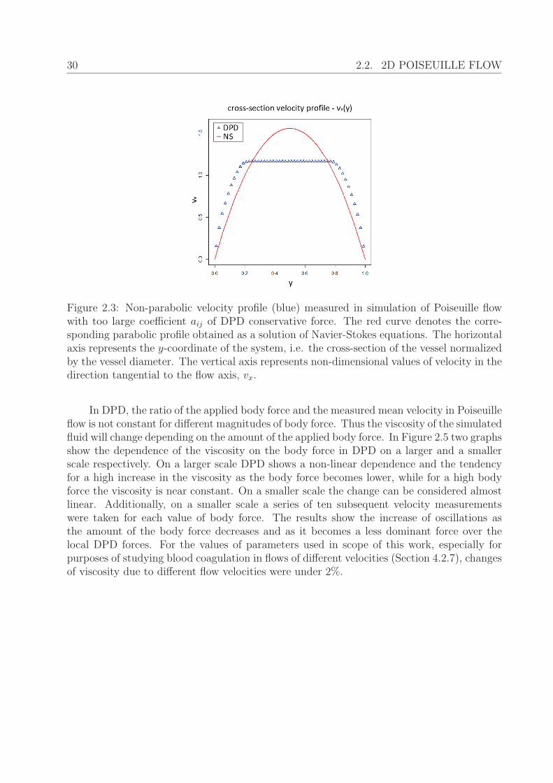
30 2.2. 2D POISEUILLE FLOW
Figure 2.3: Non-parabolic velocity profile (blue) measured in simulation of Poiseuille flowwith too large coefficient aij of DPD conservative force. The red curve denotes the corre-sponding parabolic profile obtained as a solution of Navier-Stokes equations. The horizontalaxis represents the y-coordinate of the system, i.e. the cross-section of the vessel normalizedby the vessel diameter. The vertical axis represents non-dimensional values of velocity in thedirection tangential to the flow axis, vx.
In DPD, the ratio of the applied body force and the measured mean velocity in Poiseuilleflow is not constant for different magnitudes of body force. Thus the viscosity of the simulatedfluid will change depending on the amount of the applied body force. In Figure 2.5 two graphsshow the dependence of the viscosity on the body force in DPD on a larger and a smallerscale respectively. On a larger scale DPD shows a non-linear dependence and the tendencyfor a high increase in the viscosity as the body force becomes lower, while for a high bodyforce the viscosity is near constant. On a smaller scale the change can be considered almostlinear. Additionally, on a smaller scale a series of ten subsequent velocity measurementswere taken for each value of body force. The results show the increase of oscillations asthe amount of the body force decreases and as it becomes a less dominant force over thelocal DPD forces. For the values of parameters used in scope of this work, especially forpurposes of studying blood coagulation in flows of different velocities (Section 4.2.7), changesof viscosity due to different flow velocities were under 2%.
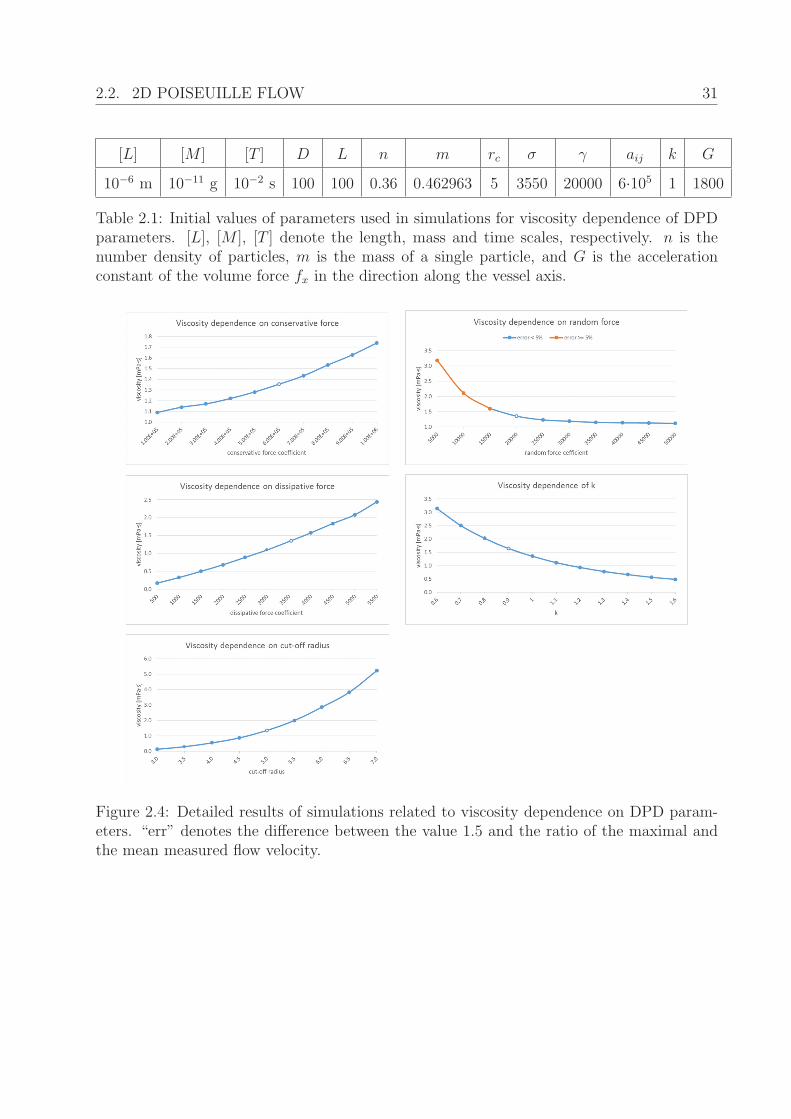
2.2. 2D POISEUILLE FLOW 31
[L] [M ] [T ] D L n m rc σ γ aij k G
10−6 m 10−11 g 10−2 s 100 100 0.36 0.462963 5 3550 20000 6·105 1 1800
Table 2.1: Initial values of parameters used in simulations for viscosity dependence of DPDparameters. [L], [M ], [T ] denote the length, mass and time scales, respectively. n is thenumber density of particles, m is the mass of a single particle, and G is the accelerationconstant of the volume force fx in the direction along the vessel axis.
Figure 2.4: Detailed results of simulations related to viscosity dependence on DPD param-eters. “err” denotes the difference between the value 1.5 and the ratio of the maximal andthe mean measured flow velocity.
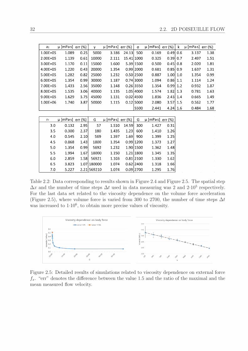
32 2.2. 2D POISEUILLE FLOW
Table 2.2: Data corresponding to results shown in Figure 2.4 and Figure 2.5. The spatial stepΔx and the number of time steps Δt used in data measuring was 2 and 2·105 respectively.For the last data set related to the viscosity dependence on the volume force acceleration(Figure 2.5), where volume force is varied from 300 to 2700, the number of time steps Δtwas increased to 1·106, to obtain more precise values of viscosity.
Figure 2.5: Detailed results of simulations related to viscosity dependence on external forcefx. “err” denotes the difference between the value 1.5 and the ratio of the maximal and themean measured flow velocity.
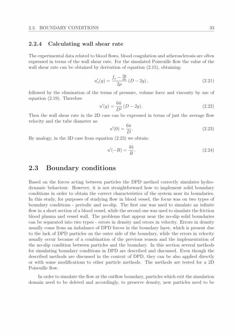
2.3. BOUNDARY CONDITIONS 33
2.2.4 Calculating wall shear rate
The experimental data related to blood flows, blood coagulation and atherosclerosis are oftenexpressed in terms of the wall shear rate. For the simulated Poiseuille flow the value of thewall shear rate can be obtained by derivation of equation (2.15), obtaining:
u′x(y) =
fx − ∂p∂x
2μ(D − 2y) , (2.21)
followed by the elimination of the terms of pressure, volume force and viscosity by use ofequation (2.19). Therefore
u′(y) =6u
D2(D − 2y) . (2.22)
Then the wall shear rate in the 2D case can be expressed in terms of just the average flowvelocity and the tube diameter as:
u′(0) =6u
D. (2.23)
By analogy, in the 3D case from equation (2.23) we obtain:
u′(−R) =4u
R. (2.24)
2.3 Boundary conditions
Based on the forces acting between particles the DPD method correctly simulates hydro-dynamic behaviour. However, it is not straightforward how to implement solid boundaryconditions in order to obtain the correct characteristics of the system near its boundaries.In this study, for purposes of studying flow in blood vessel, the focus was on two types ofboundary conditions - periodic and no-slip. The first one was used to simulate an infiniteflow in a short section of a blood vessel, while the second one was used to simulate the frictionblood plasma and vessel wall. The problems that appear near the no-slip solid boundariescan be separated into two types - errors in density and errors in velocity. Errors in densityusually come from an imbalance of DPD forces in the boundary layer, which is present dueto the lack of DPD particles on the outer side of the boundary, while the errors in velocityusually occur because of a combination of the previous reason and the implementation ofthe no-slip condition between particles and the boundary. In this section several methodsfor simulating boundary conditions in DPD are described and discussed. Even though thedescribed methods are discussed in the context of DPD, they can be also applied directlyor with some modifications to other particle methods. The methods are tested for a 2DPoiseuille flow.
In order to simulate the flow at the outflow boundary, particles which exit the simulationdomain need to be deleted and accordingly, to preserve density, new particles need to be
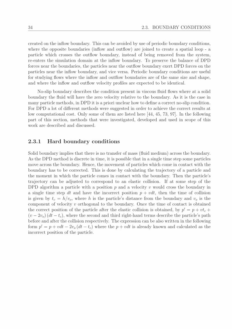
34 2.3. BOUNDARY CONDITIONS
created on the inflow boundary. This can be avoided by use of periodic boundary conditions,where the opposite boundaries (inflow and outflow) are joined to create a spatial loop - aparticle which crosses the outflow boundary, instead of being removed from the system,re-enters the simulation domain at the inflow boundary. To preserve the balance of DPDforces near the boundaries, the particles near the outflow boundary exert DPD forces on theparticles near the inflow boundary, and vice versa. Periodic boundary conditions are usefulfor studying flows where the inflow and outflow boundaries are of the same size and shape,and where the inflow and outflow velocity profiles are expected to be identical.
No-slip boundary describes the condition present in viscous fluid flows where at a solidboundary the fluid will have the zero velocity relative to the boundary. As it is the case inmany particle methods, in DPD it is a priori unclear how to define a correct no-slip condition.For DPD a lot of different methods were suggested in order to achieve the correct results atlow computational cost. Only some of them are listed here [44, 45, 73, 97]. In the followingpart of this section, methods that were investigated, developed and used in scope of thiswork are described and discussed.
2.3.1 Hard boundary conditions
Solid boundary implies that there is no transfer of mass (fluid medium) across the boundary.As the DPD method is discrete in time, it is possible that in a single time step some particlesmove across the boundary. Hence, the movement of particles which come in contact with theboundary has to be corrected. This is done by calculating the trajectory of a particle andthe moment in which the particle comes in contact with the boundary. Then the particle’strajectory can be adjusted to correspond to an elastic collision. If at some step of theDPD algorithm a particle with a position p and a velocity v would cross the boundary ina single time step dt and have the incorrect position p + vdt, then the time of collisionis given by tc = h/vo, where h is the particle’s distance from the boundary and vo is thecomponent of velocity v orthogonal to the boundary. Once the time of contact is obtainedthe correct position of the particle after the elastic collision is obtained, by p′ = p + vtc +(v − 2vo) (dt− tc), where the second and third right-hand terms describe the particle’s pathbefore and after the collision respectively. The expression can be also written in the followingform p′ = p + vdt − 2vo (dt− tc) where the p + vdt is already known and calculated as theincorrect position of the particle.
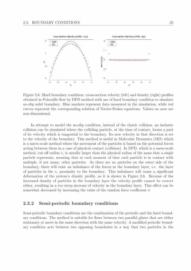
2.3. BOUNDARY CONDITIONS 35
Figure 2.6: Hard boundary condition: cross-section velocity (left) and density (right) profilesobtained in Poiseuille flow by DPD method with use of hard boundary condition to simulateno-slip solid boundary. Blue markers represent data measured in the simulation, while redcurves represent the corresponding solution of Navier-Stokes equations. Values on axes arenon-dimensional.
In attempt to model the no-slip condition, instead of the elastic collision, an inelasticcollision can be simulated where the colliding particle, at the time of contact, looses a partof its velocity which is tangential to the boundary. Its new velocity in that direction is setto the velocity of the boundary. This method is useful in Molecular Dynamics (MD) whichis a micro-scale method where the movement of the particles is based on the potential forcesacting between them in a case of physical contact (collision). In DPD, which is a meso-scalemethod, cut-off radius rc is usually larger than the physical radius of the mass that a singleparticle represents, meaning that at each moment of time each particle is in contact withmultiple, if not many, other particles. As there are no particles on the outer side of theboundary, there will exist an imbalance of the forces in the boundary layer, i.e. the layerof particles in the rc proximity to the boundary. This imbalance will cause a significantdeformation of the system’s density profile, as it is shown in Figure 2.6. Because of theincreased density of particles in the boundary layer the velocity profile cannot be correcteither, resulting in a too steep increase of velocity in the boundary layer. This effect can besomewhat decreased by increasing the value of the random force coefficient σ.
2.3.2 Semi-periodic boundary conditions
Semi-periodic boundary conditions are the combination of the periodic and the hard bound-ary conditions. The method is suitable for flows between two parallel plates that are eitherstationary or move in the same direction with the same velocity. A modified periodic bound-ary condition acts between two opposing boundaries in a way that two particles in the
36 2.3. BOUNDARY CONDITIONS
opposing boundary layers exert on each other only the component of DPD forces which isorthogonal to the boundary, while the tangential component is omitted. Additionally, thecrossing of particles over the boundaries is prevented by use of hard boundary conditions.The method produces a correct density profile due to restored balance of DPD forces inboundary layers. However, the corresponding velocity profile again suffers from a too steepincrease in the velocity in the boundary layers. This happens because particles do not collidewith the boundary often enough to produce the effect of the no-slip condition. The effectsof half periodic boundary condition shows the necessity of using boundary conditions whichdefine the areal influence on the particles, rather than just defining the behaviour for thecase of collision of particles with the boundary.
2.3.3 Estimated boundary conditions
As the problem of obtaining the correct density and velocity profiles is a result of not havingparticles on the outer side of the boundary, one way to try to resolve this problem is toestimate the effect such particles would have on a single particle in the boundary layer.The influence of the outer particles on a particle p inside of the domain will depend on thedistance of the particle p from the boundary. In other words, the closer the particle p is tothe boundary, the larger the part of the sphere around it, defined by the force cut-off radiusrc, will be outside of the domain. Let us consider a 2D case and a lower half of the circledefined by rc around some particle p. For some step dx let us fill this lower half circle withparticles pij positioned on the rectangular mesh with step dx in the following way - if rp is theposition of the particle p, then the position of particle pij is given with rij = rp + (i,−j) dx,where n = rc/dx, −n ≤ i ≤ n and 0 ≤ j ≤ n. By this definition it follows that p ≡ p00, thusthe particle p00 is not considered as a part of the mesh. The conservative and dissipativeforces that a particle pij exerts on the particle p are then given by:
FC (i, j) =a
(1− r
rc
)r
=
(a
(1− r
rc
)rx, a
(1− r
rc
)ry
)(2.25)
FD (i, j) =− γωD (r) (v · r) r
=(−γωD (r) (vxrx + vyry) rx,−γωD (r) (vxrx + vyry) ry
)=(−γωD (r)
(vxr
2x + vyrxry
),−γωD (r)
(vxrxry + vyr
2y
)), (2.26)
where r = rp − rij, r = |r|, r = r/r, vp and vij are velocities of the particles p and pijrespectively, and v = vp − vij. As all the particles pij are particles of the boundary we can
2.3. BOUNDARY CONDITIONS 37
assume that are all moving with the same velocity v. Now let us denote the components ofthe vectors in equations (2.25), (2.26) as:
XC (i, j) = a
(1− r
rc
)rx,
XDx (i, j) = −γωD(r)r2x,
XDy (i, j) = −γωD(r)rxry, (2.27)
Y C (i, j) = a
(1− h
rc
)ry,
Y Dx (i, j) = −γωDrxry,
Y Dy (i, j) = −γωDr2y.
Then it follows that:
XC(−i, j) = −XC(i, j),
XDy (−i, j) = −XD
y (i, j), (2.28)
Y Dx (−i, j) = −Y D
x (i, j),
XC(0, j) = XDy (0, j) = Y D
x (0, j) = 0.
Let us now write the influence of all particles of the mesh for which ry is greater thansome non-negative value h on the particle p:
XC(h) =∑
−n≤i≤−n
∑jdx>h
XC(i, j)
XDx (h) =
∑−n≤i≤−n
∑jdx>h
XDx (i, j),
XDy (h) =
∑−n≤i≤−n
∑jdx>h
XDy (i, j), (2.29)
Y C(h) =∑
−n≤i≤−n
∑jdx>h
Y C(i, j),
Y Dx (h) =
∑−n≤i≤−n
∑jdx>h
Y Dx (i, j),
Y Dy (h) =
∑−n≤i≤−n
∑jdx>h
Y Dy (i, j).
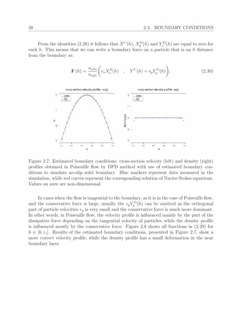
38 2.3. BOUNDARY CONDITIONS
From the identities (2.28) it follows that XC(h), XDy (h) and Y D
x (h) are equal to zero foreach h. This means that we can write a boundary force on a particle that is on h distancefrom the boundary as:
F (h) =nsimncalc
(vxX
Dx (h) , Y C(h) + vyY
Dy (h)
). (2.30)
Figure 2.7: Estimated boundary conditions: cross-section velocity (left) and density (right)profiles obtained in Poiseuille flow by DPD method with use of estimated boundary con-ditions to simulate no-slip solid boundary. Blue markers represent data measured in thesimulation, while red curves represent the corresponding solution of Navier-Stokes equations.Values on axes are non-dimensional.
In cases when the flow is tangential to the boundary, as it is in the case of Poiseuille flow,and the conservative force is large, usually the vyY
Dy (h) can be omitted as the orthogonal
part of particle velocities vy is very small and the conservative force is much more dominant.In other words, in Poiseuille flow, the velocity profile is influenced mainly by the part of thedissipative force depending on the tangential velocity of particles, while the density profileis influenced mostly by the conservative force. Figure 2.8 shows all functions in (2.29) forh ∈ [0, rc]. Results of the estimated boundary conditions, presented in Figure 2.7, show amore correct velocity profile, while the density profile has a small deformation in the nearboundary layer.
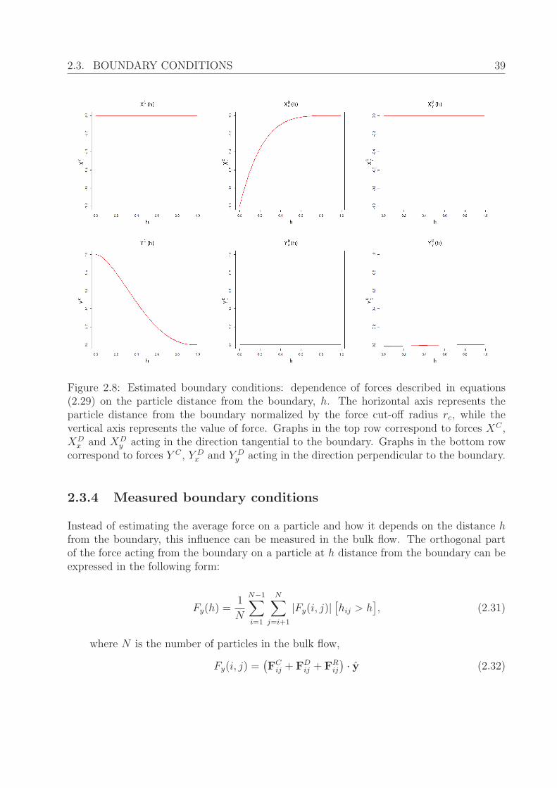
2.3. BOUNDARY CONDITIONS 39
Figure 2.8: Estimated boundary conditions: dependence of forces described in equations(2.29) on the particle distance from the boundary, h. The horizontal axis represents theparticle distance from the boundary normalized by the force cut-off radius rc, while thevertical axis represents the value of force. Graphs in the top row correspond to forces XC ,XDx and XD
y acting in the direction tangential to the boundary. Graphs in the bottom rowcorrespond to forces Y C , Y D
x and Y Dy acting in the direction perpendicular to the boundary.
2.3.4 Measured boundary conditions
Instead of estimating the average force on a particle and how it depends on the distance hfrom the boundary, this influence can be measured in the bulk flow. The orthogonal partof the force acting from the boundary on a particle at h distance from the boundary can beexpressed in the following form:
Fy(h) =1
N
N−1∑i=1
N∑j=i+1
|Fy(i, j)|[hij > h
], (2.31)
where N is the number of particles in the bulk flow,
Fy(i, j) =(FCij + FD
ij + FRij
) · y (2.32)
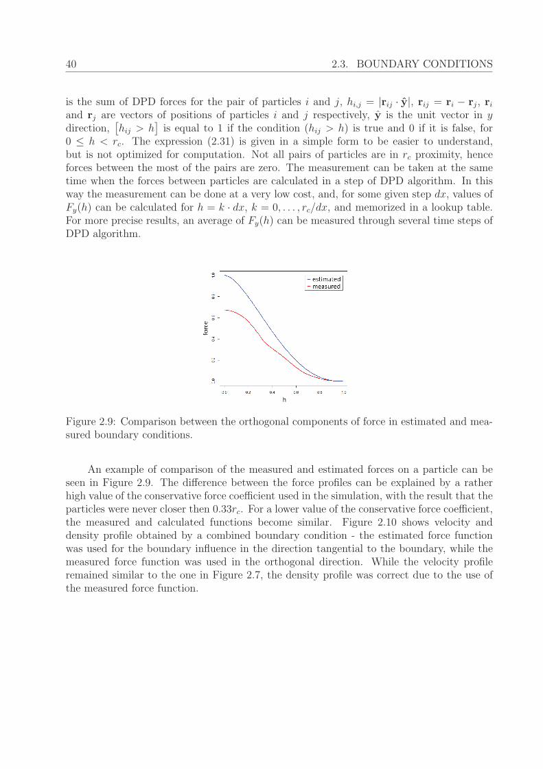
40 2.3. BOUNDARY CONDITIONS
is the sum of DPD forces for the pair of particles i and j, hi,j = |rij · y|, rij = ri − rj, riand rj are vectors of positions of particles i and j respectively, y is the unit vector in ydirection,
[hij > h
]is equal to 1 if the condition (hij > h) is true and 0 if it is false, for
0 ≤ h < rc. The expression (2.31) is given in a simple form to be easier to understand,but is not optimized for computation. Not all pairs of particles are in rc proximity, henceforces between the most of the pairs are zero. The measurement can be taken at the sametime when the forces between particles are calculated in a step of DPD algorithm. In thisway the measurement can be done at a very low cost, and, for some given step dx, values ofFy(h) can be calculated for h = k · dx, k = 0, . . . , rc/dx, and memorized in a lookup table.For more precise results, an average of Fy(h) can be measured through several time steps ofDPD algorithm.
Figure 2.9: Comparison between the orthogonal components of force in estimated and mea-sured boundary conditions.
An example of comparison of the measured and estimated forces on a particle can beseen in Figure 2.9. The difference between the force profiles can be explained by a ratherhigh value of the conservative force coefficient used in the simulation, with the result that theparticles were never closer then 0.33rc. For a lower value of the conservative force coefficient,the measured and calculated functions become similar. Figure 2.10 shows velocity anddensity profile obtained by a combined boundary condition - the estimated force functionwas used for the boundary influence in the direction tangential to the boundary, while themeasured force function was used in the orthogonal direction. While the velocity profileremained similar to the one in Figure 2.7, the density profile was correct due to the use ofthe measured force function.

2.3. BOUNDARY CONDITIONS 41
Figure 2.10: Measured boundary condition: cross-section velocity (left) and density (right)profiles obtained in Poiseuille flow by DPD method with use of a combination of measuredand estimated boundary conditions to simulate no-slip solid boundary. Measured boundarycondition was used for the part of force orthogonal to the boundary, while estimated bound-ary condition was used for the tangential part. Blue markers represent data measured in thesimulation and red curves represent the corresponding solution of Navier-Stokes equations.Values on axes are non-dimensional.
2.3.5 Mirror boundary conditions
The no-slip solid boundary is modelled in the following way: if a particle p is on a distancer < rc from the solid boundary, there exists a mirror image p′ of the particle p on the otherside of the boundary, with the velocity opposite to the velocity of particle p (vp′ ≡ −vp). Thiscan seem like adding a fair number of new particles, which can increase the simulation cost.Although the increase of computational cost cannot be completely avoided, the boundaryconditions can be efficiently implemented without any real addition of new particles. All themirrored particles are mirror images of particles which are in boundary layers of the solidboundaries. Therefore, when we calculate forces between two particles in the simulationdomain, p1 and p2, if they are both in the same boundary layer, we can calculate the forceof the imaginary particle p′1 on the particle p2 and p′2 on p1. Additionally, if particle p ison r < 1
2rc distance from the boundary, the force from p′ on p is calculated. As it is shown
in Figure 2.11, the described boundary condition produces correct profiles for both, densityand velocity.
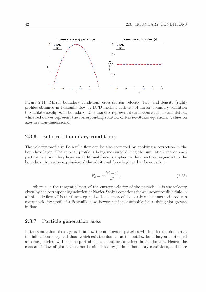
42 2.3. BOUNDARY CONDITIONS
Figure 2.11: Mirror boundary condition: cross-section velocity (left) and density (right)profiles obtained in Poiseuille flow by DPD method with use of mirror boundary conditionto simulate no-slip solid boundary. Blue markers represent data measured in the simulation,while red curves represent the corresponding solution of Navier-Stokes equations. Values onaxes are non-dimensional.
2.3.6 Enforced boundary conditions
The velocity profile in Poiseuille flow can be also corrected by applying a correction in theboundary layer. The velocity profile is being measured during the simulation and on eachparticle in a boundary layer an additional force is applied in the direction tangential to theboundary. A precise expression of the additional force is given by the equation:
Fx = m(v′ − v)
dt, (2.33)
where v is the tangential part of the current velocity of the particle, v′ is the velocitygiven by the corresponding solution of Navier-Stokes equations for an incompressible fluid ina Poiseuille flow, dt is the time step and m is the mass of the particle. The method producescorrect velocity profile for Poiseuille flow, however it is not suitable for studying clot growthin flow.
2.3.7 Particle generation area
In the simulation of clot growth in flow the numbers of platelets which enter the domain atthe inflow boundary and those which exit the domain at the outflow boundary are not equalas some platelets will become part of the clot and be contained in the domain. Hence, theconstant inflow of platelets cannot be simulated by periodic boundary conditions, and more
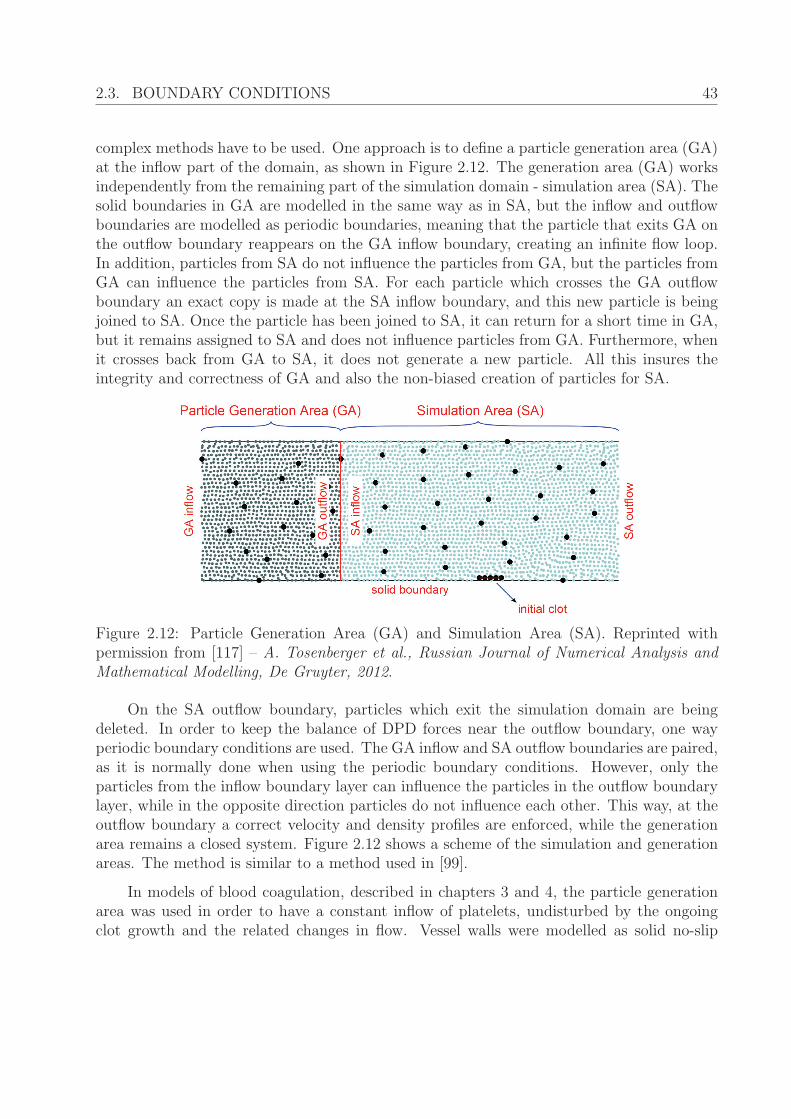
2.3. BOUNDARY CONDITIONS 43
complex methods have to be used. One approach is to define a particle generation area (GA)at the inflow part of the domain, as shown in Figure 2.12. The generation area (GA) worksindependently from the remaining part of the simulation domain - simulation area (SA). Thesolid boundaries in GA are modelled in the same way as in SA, but the inflow and outflowboundaries are modelled as periodic boundaries, meaning that the particle that exits GA onthe outflow boundary reappears on the GA inflow boundary, creating an infinite flow loop.In addition, particles from SA do not influence the particles from GA, but the particles fromGA can influence the particles from SA. For each particle which crosses the GA outflowboundary an exact copy is made at the SA inflow boundary, and this new particle is beingjoined to SA. Once the particle has been joined to SA, it can return for a short time in GA,but it remains assigned to SA and does not influence particles from GA. Furthermore, whenit crosses back from GA to SA, it does not generate a new particle. All this insures theintegrity and correctness of GA and also the non-biased creation of particles for SA.
Figure 2.12: Particle Generation Area (GA) and Simulation Area (SA). Reprinted withpermission from [117] – A. Tosenberger et al., Russian Journal of Numerical Analysis andMathematical Modelling, De Gruyter, 2012.
On the SA outflow boundary, particles which exit the simulation domain are beingdeleted. In order to keep the balance of DPD forces near the outflow boundary, one wayperiodic boundary conditions are used. The GA inflow and SA outflow boundaries are paired,as it is normally done when using the periodic boundary conditions. However, only theparticles from the inflow boundary layer can influence the particles in the outflow boundarylayer, while in the opposite direction particles do not influence each other. This way, at theoutflow boundary a correct velocity and density profiles are enforced, while the generationarea remains a closed system. Figure 2.12 shows a scheme of the simulation and generationareas. The method is similar to a method used in [99].
In models of blood coagulation, described in chapters 3 and 4, the particle generationarea was used in order to have a constant inflow of platelets, undisturbed by the ongoingclot growth and the related changes in flow. Vessel walls were modelled as solid no-slip
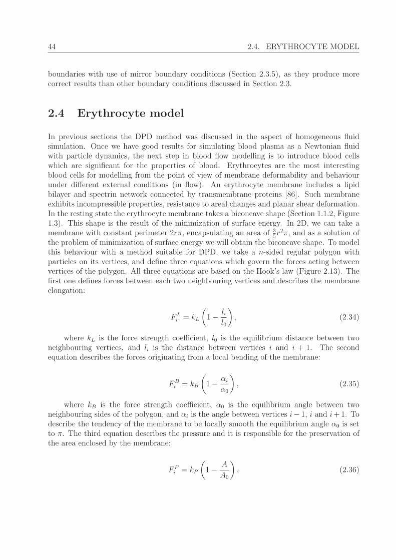
44 2.4. ERYTHROCYTE MODEL
boundaries with use of mirror boundary conditions (Section 2.3.5), as they produce morecorrect results than other boundary conditions discussed in Section 2.3.
2.4 Erythrocyte model
In previous sections the DPD method was discussed in the aspect of homogeneous fluidsimulation. Once we have good results for simulating blood plasma as a Newtonian fluidwith particle dynamics, the next step in blood flow modelling is to introduce blood cellswhich are significant for the properties of blood. Erythrocytes are the most interestingblood cells for modelling from the point of view of membrane deformability and behaviourunder different external conditions (in flow). An erythrocyte membrane includes a lipidbilayer and spectrin network connected by transmembrane proteins [86]. Such membraneexhibits incompressible properties, resistance to areal changes and planar shear deformation.In the resting state the erythrocyte membrane takes a biconcave shape (Section 1.1.2, Figure1.3). This shape is the result of the minimization of surface energy. In 2D, we can take amembrane with constant perimeter 2rπ, encapsulating an area of 3
5r2π, and as a solution of
the problem of minimization of surface energy we will obtain the biconcave shape. To modelthis behaviour with a method suitable for DPD, we take a n-sided regular polygon withparticles on its vertices, and define three equations which govern the forces acting betweenvertices of the polygon. All three equations are based on the Hook’s law (Figure 2.13). Thefirst one defines forces between each two neighbouring vertices and describes the membraneelongation:
FLi = kL
(1− li
l0
), (2.34)
where kL is the force strength coefficient, l0 is the equilibrium distance between twoneighbouring vertices, and li is the distance between vertices i and i + 1. The secondequation describes the forces originating from a local bending of the membrane:
FBi = kB
(1− αi
α0
), (2.35)
where kB is the force strength coefficient, α0 is the equilibrium angle between twoneighbouring sides of the polygon, and αi is the angle between vertices i− 1, i and i+1. Todescribe the tendency of the membrane to be locally smooth the equilibrium angle α0 is setto π. The third equation describes the pressure and it is responsible for the preservation ofthe area enclosed by the membrane:
F Pi = kP
(1− A
A0
), (2.36)
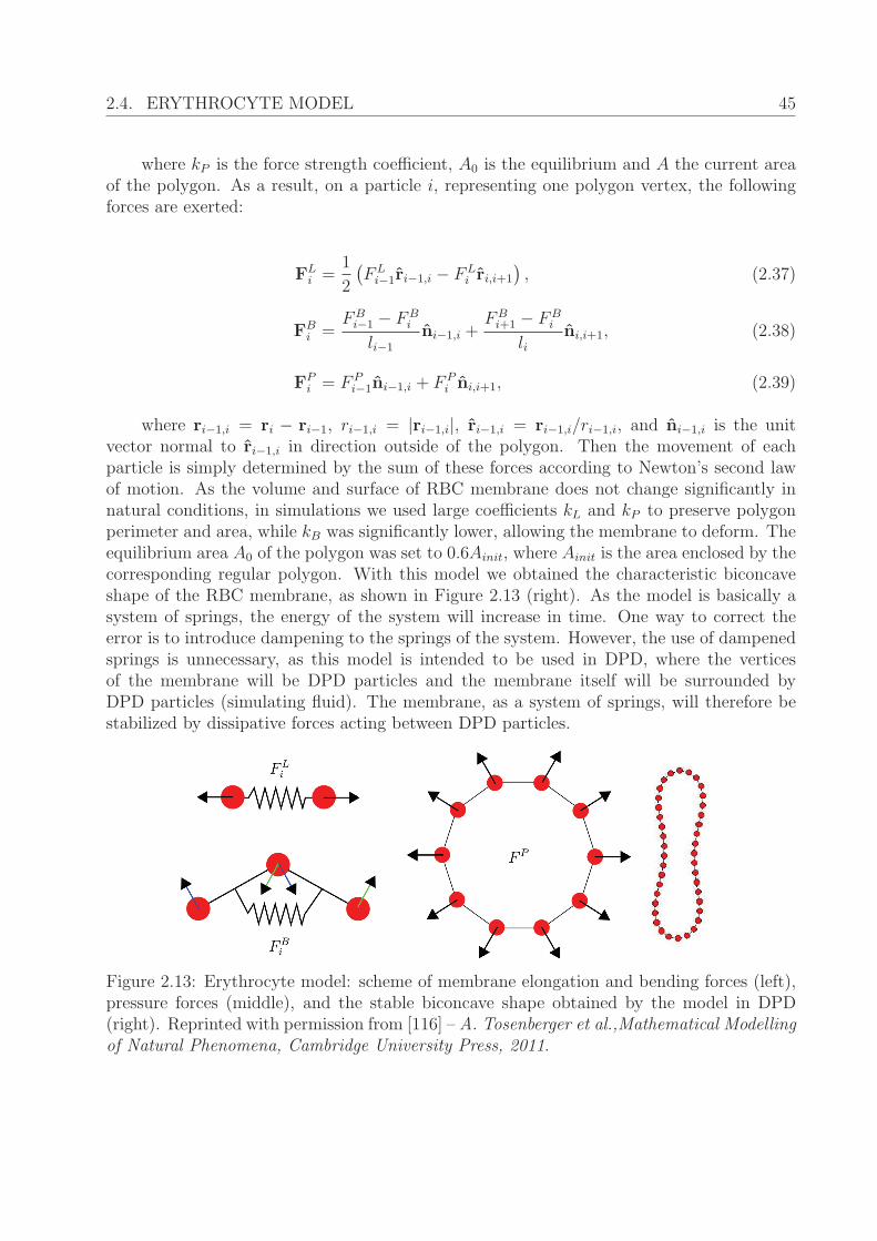
2.4. ERYTHROCYTE MODEL 45
where kP is the force strength coefficient, A0 is the equilibrium and A the current areaof the polygon. As a result, on a particle i, representing one polygon vertex, the followingforces are exerted:
FLi =
1
2
(FLi−1ri−1,i − FL
i ri,i+1
), (2.37)
FBi =
FBi−1 − FB
i
li−1
ni−1,i +FBi+1 − FB
i
lini,i+1, (2.38)
FPi = F P
i−1ni−1,i + F Pi ni,i+1, (2.39)
where ri−1,i = ri − ri−1, ri−1,i = |ri−1,i|, ri−1,i = ri−1,i/ri−1,i, and ni−1,i is the unitvector normal to ri−1,i in direction outside of the polygon. Then the movement of eachparticle is simply determined by the sum of these forces according to Newton’s second lawof motion. As the volume and surface of RBC membrane does not change significantly innatural conditions, in simulations we used large coefficients kL and kP to preserve polygonperimeter and area, while kB was significantly lower, allowing the membrane to deform. Theequilibrium area A0 of the polygon was set to 0.6Ainit, where Ainit is the area enclosed by thecorresponding regular polygon. With this model we obtained the characteristic biconcaveshape of the RBC membrane, as shown in Figure 2.13 (right). As the model is basically asystem of springs, the energy of the system will increase in time. One way to correct theerror is to introduce dampening to the springs of the system. However, the use of dampenedsprings is unnecessary, as this model is intended to be used in DPD, where the verticesof the membrane will be DPD particles and the membrane itself will be surrounded byDPD particles (simulating fluid). The membrane, as a system of springs, will therefore bestabilized by dissipative forces acting between DPD particles.
Figure 2.13: Erythrocyte model: scheme of membrane elongation and bending forces (left),pressure forces (middle), and the stable biconcave shape obtained by the model in DPD(right). Reprinted with permission from [116] – A. Tosenberger et al.,Mathematical Modellingof Natural Phenomena, Cambridge University Press, 2011.
46 2.4. ERYTHROCYTE MODEL
2.4.1 Capillary flow
In order to test the behaviour of the erythrocyte model coupled with DPD we simulated theflow in a capillary of diameter 10μm with one erythrocyte starting in the resting biconcaveshape turned orthogonally to the flow axis. It is observed that in such situations the erythro-cyte undergoes a change from its natural biconcave shape to the so-called parachute shapefollowing the parabolic velocity profile. The described behaviour obtained in DPD simula-tion is shown in Figure 2.14. For some time the erythrocyte remained in the parachute shapeand in the position orthogonal to the flow axis. However, this was not the stable state of theerythrocyte, and the erythrocyte eventually turned in the direction of the flow and regainedthe biconcave shape. Similar behaviours were studied in [89, 101, 104].
Figure 2.14: Erythrocyte model: development of the parachute shape in a narrow Poiseuilleflow. Reprinted with permission from [116] – A. Tosenberger et al.,Mathematical Modellingof Natural Phenomena, Cambridge University Press, 2011.
2.4.2 3D model
In 3D the membrane is represented as a two-dimensional network of particles as describedin [15, 16]. Similar to the 2D case, membrane particles are connected by springs (modelledby Hooke’s law) to form an irregular polyhedron with triangular sides. Forces acting to themembrane particles are chosen analogically to [63]. The first force acts between any twoneighbouring vertices and describes the ability of the corresponding joint to elongate:
Fs = ks
(1− l
l0
)τ, (2.40)
where l is the length of joint between two vertices, l0 is the equilibrium length, and ks isthe stiffness coefficient, τ is the unit vector which is co-directional with the vector connectingtwo neighbouring particles.
To express areal incompressibility the force resisting to every triangular element areachange is introduced:
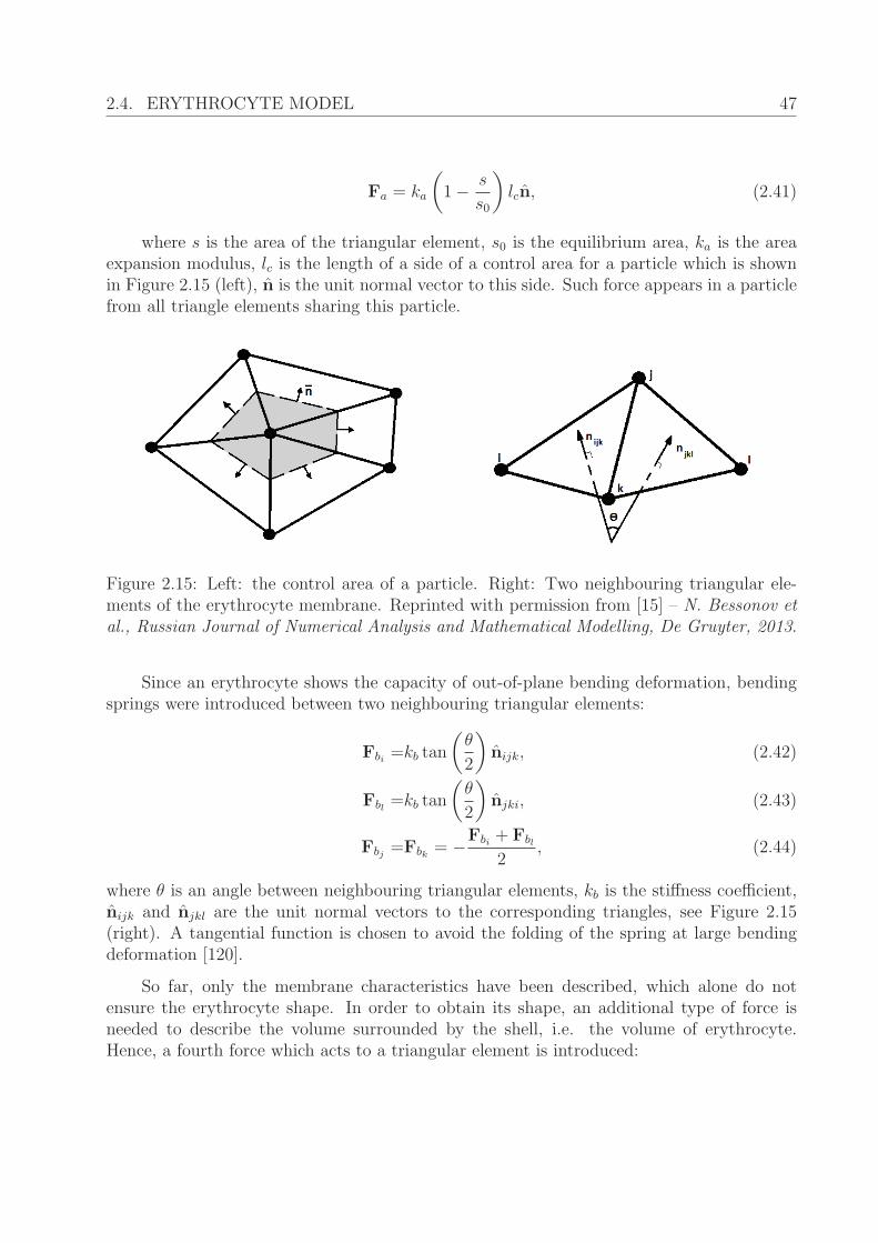
2.4. ERYTHROCYTE MODEL 47
Fa = ka
(1− s
s0
)lcn, (2.41)
where s is the area of the triangular element, s0 is the equilibrium area, ka is the areaexpansion modulus, lc is the length of a side of a control area for a particle which is shownin Figure 2.15 (left), n is the unit normal vector to this side. Such force appears in a particlefrom all triangle elements sharing this particle.
Figure 2.15: Left: the control area of a particle. Right: Two neighbouring triangular ele-ments of the erythrocyte membrane. Reprinted with permission from [15] – N. Bessonov etal., Russian Journal of Numerical Analysis and Mathematical Modelling, De Gruyter, 2013.
Since an erythrocyte shows the capacity of out-of-plane bending deformation, bendingsprings were introduced between two neighbouring triangular elements:
Fbi =kb tan
(θ
2
)nijk, (2.42)
Fbl =kb tan
(θ
2
)njki, (2.43)
Fbj =Fbk = −Fbi + Fbl
2, (2.44)
where θ is an angle between neighbouring triangular elements, kb is the stiffness coefficient,nijk and njkl are the unit normal vectors to the corresponding triangles, see Figure 2.15(right). A tangential function is chosen to avoid the folding of the spring at large bendingdeformation [120].
So far, only the membrane characteristics have been described, which alone do notensure the erythrocyte shape. In order to obtain its shape, an additional type of force isneeded to describe the volume surrounded by the shell, i.e. the volume of erythrocyte.Hence, a fourth force which acts to a triangular element is introduced:
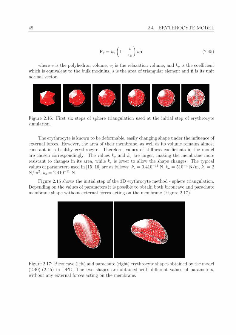
48 2.4. ERYTHROCYTE MODEL
Fv = kv
(1− v
v0
)sn, (2.45)
where v is the polyhedron volume, v0 is the relaxation volume, and kv is the coefficientwhich is equivalent to the bulk modulus, s is the area of triangular element and n is its unitnormal vector.
Figure 2.16: First six steps of sphere triangulation used at the initial step of erythrocytesimulation.
The erythrocyte is known to be deformable, easily changing shape under the influence ofexternal forces. However, the area of their membrane, as well as its volume remains almostconstant in a healthy erythrocyte. Therefore, values of stiffness coefficients in the modelare chosen correspondingly. The values kv and ka are larger, making the membrane moreresistant to changes in its area, while ks is lower to allow the shape changes. The typicalvalues of parameters used in [15, 16] are as follows: ks = 0.410−11 N, ka = 510−4 N/m, kv = 2N/m2, kb = 2.410−11 N.
Figure 2.16 shows the initial step of the 3D erythrocyte method - sphere triangulation.Depending on the values of parameters it is possible to obtain both biconcave and parachutemembrane shape without external forces acting on the membrane (Figure 2.17).
Figure 2.17: Biconcave (left) and parachute (right) erythrocyte shapes obtained by the model(2.40)-(2.45) in DPD. The two shapes are obtained with different values of parameters,without any external forces acting on the membrane.
49
Chapter 3
Discrete model of platelet aggregationin flow
3.1 Description
In this section a discrete model of platelet aggregation in blood plasma flow is described.It serves as the first step towards the development of a blood coagulation model. In thismodel we do not consider the blood coagulation pathways. DPD method is used to describeblood plasma flow inside a 2D longitudinal cross-section of a blood vessel. Platelets are alsomodelled as soft DPD particles, similar to the plasma particles. The radius and mass of allparticles (plasma and platelets) are chosen to correspond to the physical size and the mass ofplatelets. In our simulation the physical radius is set to 1μm and the mass is chosen in such away that the particle density corresponds to the density of the blood plasma (≈ 103kg/m3).The interactions between all particles are then governed by DPD as described in Section2.1 with additional adhesion force acting between aggregated platelets. By virtue of clotmechanical properties [19, 54, 106, 126], the adhesion force is modelled as a pairwise forcebetween two platelets expressed in the form of Hooke’s law:
FAij = kA
(1− rij
dC
)rij, (3.1)
where kA is the force strength constant and dC is the force relaxation distance which isequal to two times the physical radius of a platelet. As binding of platelets occurs due totheir surface adhesion receptors, two platelets in a flow connect when they come in physicalcontact, i.e. rij ≤ dC (connection criterium). Platelets remain connected until their distancedoes not exceed some critical value dD (disconnection criterium) which is greater then dC .In discrete model simulations dD was set to 1.5 times of the platelet diameter.
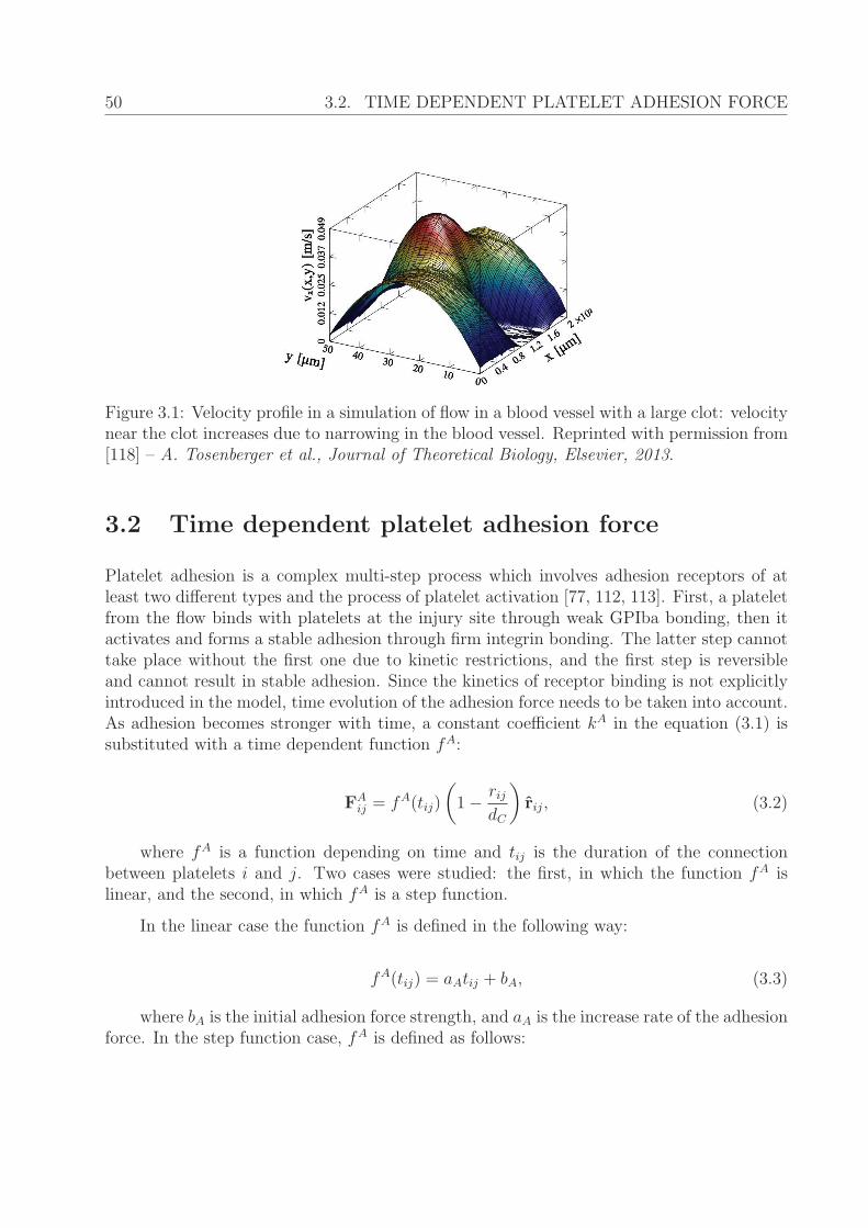
50 3.2. TIME DEPENDENT PLATELET ADHESION FORCE
Figure 3.1: Velocity profile in a simulation of flow in a blood vessel with a large clot: velocitynear the clot increases due to narrowing in the blood vessel. Reprinted with permission from[118] – A. Tosenberger et al., Journal of Theoretical Biology, Elsevier, 2013.
3.2 Time dependent platelet adhesion force
Platelet adhesion is a complex multi-step process which involves adhesion receptors of atleast two different types and the process of platelet activation [77, 112, 113]. First, a plateletfrom the flow binds with platelets at the injury site through weak GPIba bonding, then itactivates and forms a stable adhesion through firm integrin bonding. The latter step cannottake place without the first one due to kinetic restrictions, and the first step is reversibleand cannot result in stable adhesion. Since the kinetics of receptor binding is not explicitlyintroduced in the model, time evolution of the adhesion force needs to be taken into account.As adhesion becomes stronger with time, a constant coefficient kA in the equation (3.1) issubstituted with a time dependent function fA:
FAij = fA(tij)
(1− rij
dC
)rij, (3.2)
where fA is a function depending on time and tij is the duration of the connectionbetween platelets i and j. Two cases were studied: the first, in which the function fA islinear, and the second, in which fA is a step function.
In the linear case the function fA is defined in the following way:
fA(tij) = aAtij + bA, (3.3)
where bA is the initial adhesion force strength, and aA is the increase rate of the adhesionforce. In the step function case, fA is defined as follows:
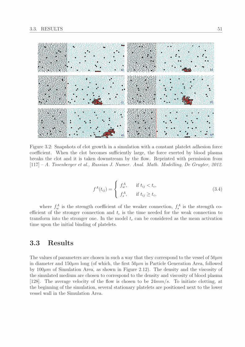
3.3. RESULTS 51
Figure 3.2: Snapshots of clot growth in a simulation with a constant platelet adhesion forcecoefficient. When the clot becomes sufficiently large, the force exerted by blood plasmabreaks the clot and it is taken downstream by the flow. Reprinted with permission from[117] – A. Tosenberger et al., Russian J. Numer. Anal. Math. Modelling, De Gruyter, 2012.
fA(tij) =
⎧⎨⎩ fAw , if tij < tc,
fAs , if tij ≥ tc,(3.4)
where fAw is the strength coefficient of the weaker connection, fAs is the strength co-efficient of the stronger connection and tc is the time needed for the weak connection totransform into the stronger one. In the model tc can be considered as the mean activationtime upon the initial binding of platelets.
3.3 Results
The values of parameters are chosen in such a way that they correspond to the vessel of 50μmin diameter and 150μm long (of which, the first 50μm is Particle Generation Area, followedby 100μm of Simulation Area, as shown in Figure 2.12). The density and the viscosity ofthe simulated medium are chosen to correspond to the density and viscosity of blood plasma[128]. The average velocity of the flow is chosen to be 24mm/s. To initiate clotting, atthe beginning of the simulation, several stationary platelets are positioned next to the lowervessel wall in the Simulation Area.
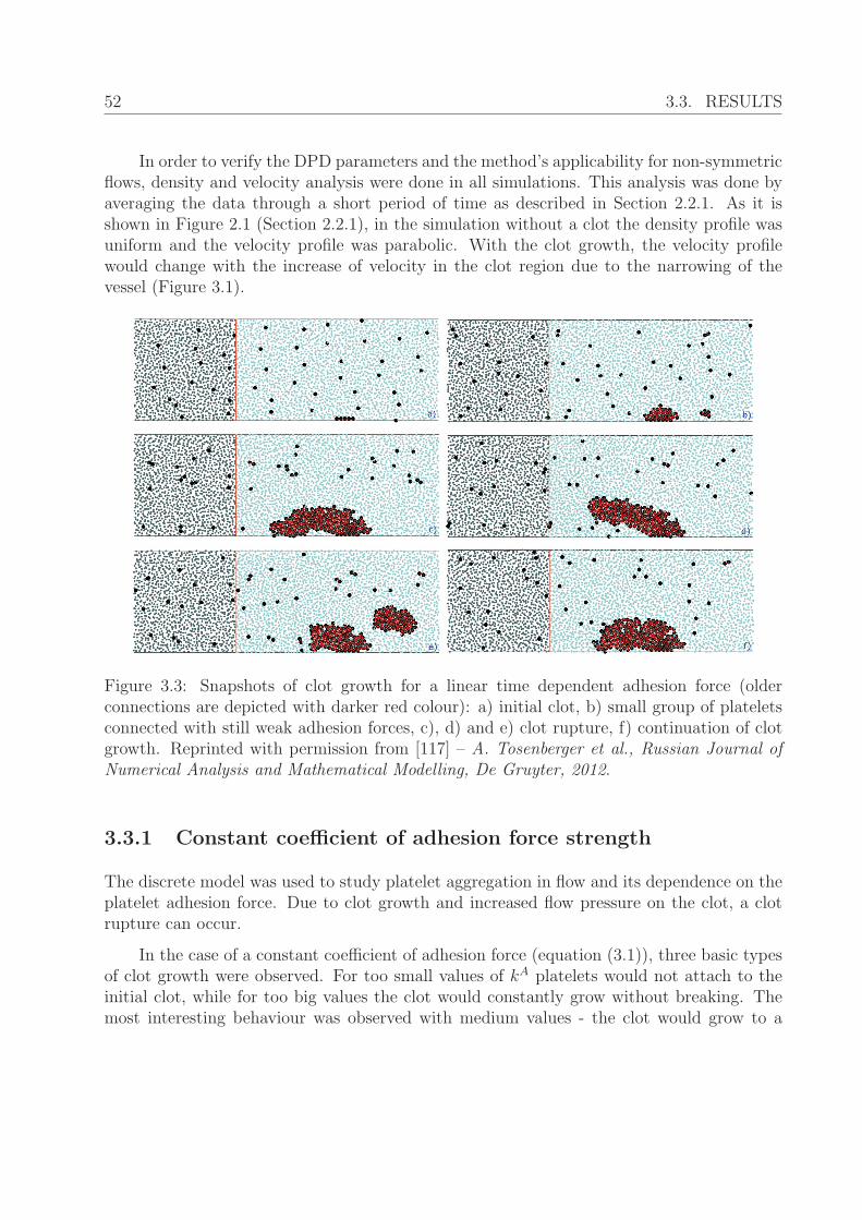
52 3.3. RESULTS
In order to verify the DPD parameters and the method’s applicability for non-symmetricflows, density and velocity analysis were done in all simulations. This analysis was done byaveraging the data through a short period of time as described in Section 2.2.1. As it isshown in Figure 2.1 (Section 2.2.1), in the simulation without a clot the density profile wasuniform and the velocity profile was parabolic. With the clot growth, the velocity profilewould change with the increase of velocity in the clot region due to the narrowing of thevessel (Figure 3.1).
Figure 3.3: Snapshots of clot growth for a linear time dependent adhesion force (olderconnections are depicted with darker red colour): a) initial clot, b) small group of plateletsconnected with still weak adhesion forces, c), d) and e) clot rupture, f) continuation of clotgrowth. Reprinted with permission from [117] – A. Tosenberger et al., Russian Journal ofNumerical Analysis and Mathematical Modelling, De Gruyter, 2012.
3.3.1 Constant coefficient of adhesion force strength
The discrete model was used to study platelet aggregation in flow and its dependence on theplatelet adhesion force. Due to clot growth and increased flow pressure on the clot, a clotrupture can occur.
In the case of a constant coefficient of adhesion force (equation (3.1)), three basic typesof clot growth were observed. For too small values of kA platelets would not attach to theinitial clot, while for too big values the clot would constantly grow without breaking. Themost interesting behaviour was observed with medium values - the clot would grow to a
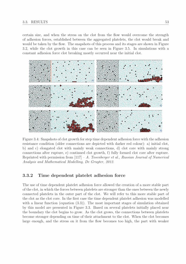
3.3. RESULTS 53
certain size, and when the stress on the clot from the flow would overcome the strengthof adhesion forces, established between the aggregated platelets, the clot would break andwould be taken by the flow. The snapshots of this process and its stages are shown in Figure3.2, while the clot growth in this case can be seen in Figure 3.5. In simulations with aconstant adhesion force clot breaking mostly occurred near the initial clot.
Figure 3.4: Snapshots of clot growth for step time dependent adhesion force with the adhesionresistance condition (older connections are depicted with darker red colour): a) initial clot,b) and c) elongated clot with mainly weak connections, d) clot core with mainly strongconnections after rupture, e) continued clot growth, f) fully formed clot core after rupture.Reprinted with permission from [117] – A. Tosenberger et al., Russian Journal of NumericalAnalysis and Mathematical Modelling, De Gruyter, 2012.
3.3.2 Time dependent platelet adhesion force
The use of time dependent platelet adhesion force allowed the creation of a more stable partof the clot, in which the forces between platelets are stronger than the ones between the newlyconnected platelets in the outer part of the clot. We will refer to this more stable part ofthe clot as the clot core. In the first case the time dependent platelet adhesion was modelledwith a linear function (equation (3.3)). The most important stages of simulation obtainedby this model are presented in Figure 3.3. Based on several platelets initially placed nearthe boundary the clot begins to grow. As the clot grows, the connections between plateletsbecome stronger depending on time of their attachment to the clot. When the clot becomeslarge enough, and the stress on it from the flow becomes too high, the part with weaker
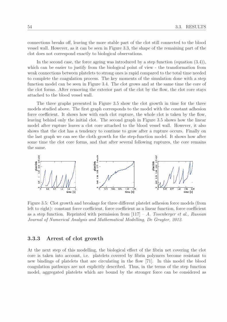
54 3.3. RESULTS
connections breaks off, leaving the more stable part of the clot still connected to the bloodvessel wall. However, as it can be seen in Figure 3.3, the shape of the remaining part of theclot does not correspond exactly to biological observations.
In the second case, the force ageing was introduced by a step function (equation (3.4)),which can be easier to justify from the biological point of view - the transformation fromweak connections between platelets to strong ones is rapid compared to the total time neededto complete the coagulation process. The key moments of the simulation done with a stepfunction model can be seen in Figure 3.4. The clot grows and at the same time the core ofthe clot forms. After removing the exterior part of the clot by the flow, the clot core staysattached to the blood vessel wall.
The three graphs presented in Figure 3.5 show the clot growth in time for the threemodels studied above. The first graph corresponds to the model with the constant adhesionforce coefficient. It shows how with each clot rupture, the whole clot is taken by the flow,leaving behind only the initial clot. The second graph in Figure 3.5 shows how the linearmodel after rupture leaves a clot core attached to the blood vessel wall. However, it alsoshows that the clot has a tendency to continue to grow after a rupture occurs. Finally onthe last graph we can see the cloth growth for the step-function model. It shows how aftersome time the clot core forms, and that after several following ruptures, the core remainsthe same.
Figure 3.5: Clot growth and breakage for three different platelet adhesion force models (fromleft to right): constant force coefficient, force coefficient as a linear function, force coefficientas a step function. Reprinted with permission from [117] – A. Tosenberger et al., RussianJournal of Numerical Analysis and Mathematical Modelling, De Gruyter, 2012.
3.3.3 Arrest of clot growth
At the next step of this modelling, the biological effect of the fibrin net covering the clotcore is taken into account, i.e. platelets covered by fibrin polymers become resistant tonew bindings of platelets that are circulating in the flow [71]. In this model the bloodcoagulation pathways are not explicitly described. Thus, in the terms of the step functionmodel, aggregated platelets which are bound by the stronger force can be considered as
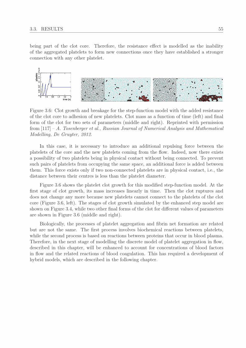
3.3. RESULTS 55
being part of the clot core. Therefore, the resistance effect is modelled as the inabilityof the aggregated platelets to form new connections once they have established a strongerconnection with any other platelet.
Figure 3.6: Clot growth and breakage for the step-function model with the added resistanceof the clot core to adhesion of new platelets. Clot mass as a function of time (left) and finalform of the clot for two sets of parameters (middle and right). Reprinted with permissionfrom [117] – A. Tosenberger et al., Russian Journal of Numerical Analysis and MathematicalModelling, De Gruyter, 2012.
In this case, it is necessary to introduce an additional repulsing force between theplatelets of the core and the new platelets coming from the flow. Indeed, now there existsa possibility of two platelets being in physical contact without being connected. To preventsuch pairs of platelets from occupying the same space, an additional force is added betweenthem. This force exists only if two non-connected platelets are in physical contact, i.e., thedistance between their centres is less than the platelet diameter.
Figure 3.6 shows the platelet clot growth for this modified step-function model. At thefirst stage of clot growth, its mass increases linearly in time. Then the clot ruptures anddoes not change any more because new platelets cannot connect to the platelets of the clotcore (Figure 3.6, left). The stages of clot growth simulated by the enhanced step model areshown on Figure 3.4, while two other final forms of the clot for different values of parametersare shown in Figure 3.6 (middle and right).
Biologically, the processes of platelet aggregation and fibrin net formation are relatedbut are not the same. The first process involves biochemical reactions between platelets,while the second process is based on reactions between proteins that occur in blood plasma.Therefore, in the next stage of modelling the discrete model of platelet aggregation in flow,described in this chapter, will be enhanced to account for concentrations of blood factorsin flow and the related reactions of blood coagulation. This has required a development ofhybrid models, which are described in the following chapter.

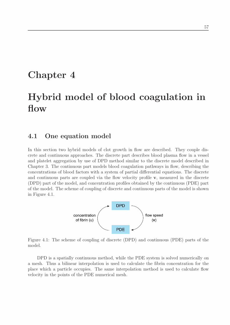
57
Chapter 4
Hybrid model of blood coagulation inflow
4.1 One equation model
In this section two hybrid models of clot growth in flow are described. They couple dis-crete and continuous approaches. The discrete part describes blood plasma flow in a vesseland platelet aggregation by use of DPD method similar to the discrete model described inChapter 3. The continuous part models blood coagulation pathways in flow, describing theconcentrations of blood factors with a system of partial differential equations. The discreteand continuous parts are coupled via the flow velocity profile v, measured in the discrete(DPD) part of the model, and concentration profiles obtained by the continuous (PDE) partof the model. The scheme of coupling of discrete and continuous parts of the model is shownin Figure 4.1.
Figure 4.1: The scheme of coupling of discrete (DPD) and continuous (PDE) parts of themodel.
DPD is a spatially continuous method, while the PDE system is solved numerically ona mesh. Thus a bilinear interpolation is used to calculate the fibrin concentration for theplace which a particle occupies. The same interpolation method is used to calculate flowvelocity in the points of the PDE numerical mesh.
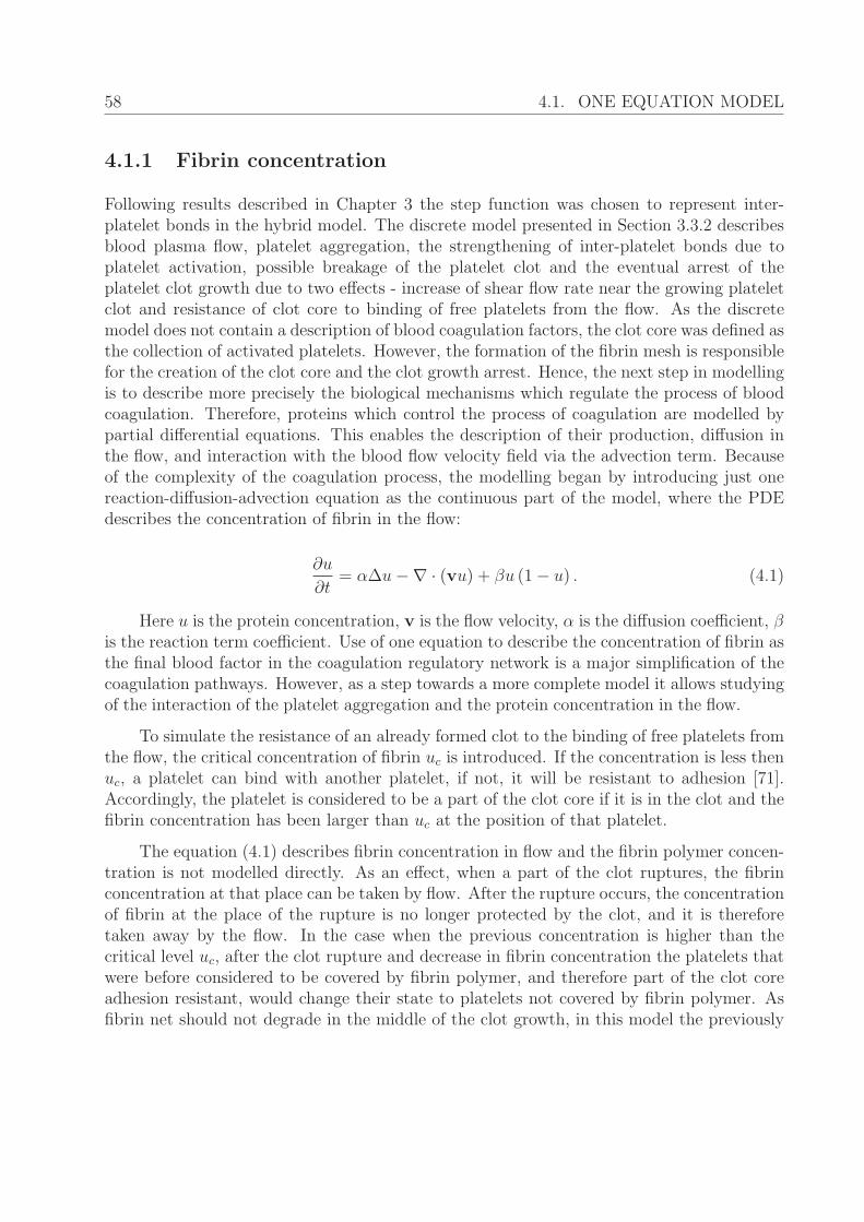
58 4.1. ONE EQUATION MODEL
4.1.1 Fibrin concentration
Following results described in Chapter 3 the step function was chosen to represent inter-platelet bonds in the hybrid model. The discrete model presented in Section 3.3.2 describesblood plasma flow, platelet aggregation, the strengthening of inter-platelet bonds due toplatelet activation, possible breakage of the platelet clot and the eventual arrest of theplatelet clot growth due to two effects - increase of shear flow rate near the growing plateletclot and resistance of clot core to binding of free platelets from the flow. As the discretemodel does not contain a description of blood coagulation factors, the clot core was defined asthe collection of activated platelets. However, the formation of the fibrin mesh is responsiblefor the creation of the clot core and the clot growth arrest. Hence, the next step in modellingis to describe more precisely the biological mechanisms which regulate the process of bloodcoagulation. Therefore, proteins which control the process of coagulation are modelled bypartial differential equations. This enables the description of their production, diffusion inthe flow, and interaction with the blood flow velocity field via the advection term. Becauseof the complexity of the coagulation process, the modelling began by introducing just onereaction-diffusion-advection equation as the continuous part of the model, where the PDEdescribes the concentration of fibrin in the flow:
∂u
∂t= αΔu−∇ · (vu) + βu (1− u) . (4.1)
Here u is the protein concentration, v is the flow velocity, α is the diffusion coefficient, βis the reaction term coefficient. Use of one equation to describe the concentration of fibrin asthe final blood factor in the coagulation regulatory network is a major simplification of thecoagulation pathways. However, as a step towards a more complete model it allows studyingof the interaction of the platelet aggregation and the protein concentration in the flow.
To simulate the resistance of an already formed clot to the binding of free platelets fromthe flow, the critical concentration of fibrin uc is introduced. If the concentration is less thenuc, a platelet can bind with another platelet, if not, it will be resistant to adhesion [71].Accordingly, the platelet is considered to be a part of the clot core if it is in the clot and thefibrin concentration has been larger than uc at the position of that platelet.
The equation (4.1) describes fibrin concentration in flow and the fibrin polymer concen-tration is not modelled directly. As an effect, when a part of the clot ruptures, the fibrinconcentration at that place can be taken by flow. After the rupture occurs, the concentrationof fibrin at the place of the rupture is no longer protected by the clot, and it is thereforetaken away by the flow. In the case when the previous concentration is higher than thecritical level uc, after the clot rupture and decrease in fibrin concentration the platelets thatwere before considered to be covered by fibrin polymer, and therefore part of the clot coreadhesion resistant, would change their state to platelets not covered by fibrin polymer. Asfibrin net should not degrade in the middle of the clot growth, in this model the previously
4.1. ONE EQUATION MODEL 59
Figure 4.2: Clot structure. Connections between platelets are shown as intervals betweentheir centers - red lines correspond to weak connections, yellow to strong ones. Dark greenplatelets are covered by fibrin. Reprinted with permission from [118] – A. Tosenberger etal., Journal of Theoretical Biology, Elsevier, 2013.
described situation is avoided by use of platelet memory - once the platelet has been coveredby fibrin polymer (concentration higher that uc) it will remain in this state independentlyof the future level of fibrin.
4.1.2 Clot growth
In simulations with the first hybrid model the values of parameters were chosen in such away that they correspond to a vessel of 50μm in diameter and 150μm long. The densityand the viscosity of the simulated medium were chosen to correspond to the density andviscosity of blood plasma [128] (≈ 1.24mPa·s). The average velocity of the flow is chosen tobe 24mm/s. As in the discrete model, at the beginning of the simulation several stationaryplatelets are positioned next to the lower vessel wall in order to initiate platelet aggregation.As it was the case in the discrete model the size of all DPD particles was set to correspond tothe size of platelets (≈ 1μm in diameter). Figure 4.2 shows a typical clot structure obtainedin simulations. There are two types of platelet connections: weak (red lines between theircenters) and strong (yellow lines). Strong connections appear if a platelet has already weakconnections during some time. Hence platelet activation and emergence of strong connectionsis modelled as a time delay. The disconnection distance dD for inter-platelet connections wasset to 1.3 times of the platelet diameter. Platelets covered by fibrin are shown with darkgreen color, while platelets not covered by fibrin with light green.
Several stages of the clot growth and the evolution of the fibrin concentration profileprotected by the clot are shown in Figure 4.3 and Figure 4.4. In the beginning of clot growth,platelets aggregate at the injury site due to weak connections (Figure 4.3, a). The injury siteis modelled as several platelets attached to the vessel wall. They initiate clot growth. Sincethe flow velocity is sufficiently high, the concentration u of fibrin remains low (Figure 4.4,a). The platelet clot continues to grow due to weak connections and the flow speed inside itdecreases. It makes it possible for the coagulation reaction to start, and fibrin concentration
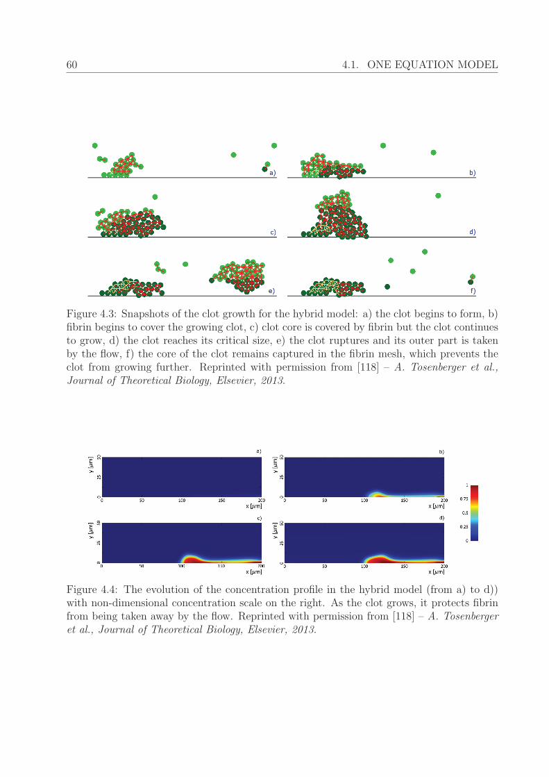
60 4.1. ONE EQUATION MODEL
Figure 4.3: Snapshots of the clot growth for the hybrid model: a) the clot begins to form, b)fibrin begins to cover the growing clot, c) clot core is covered by fibrin but the clot continuesto grow, d) the clot reaches its critical size, e) the clot ruptures and its outer part is takenby the flow, f) the core of the clot remains captured in the fibrin mesh, which prevents theclot from growing further. Reprinted with permission from [118] – A. Tosenberger et al.,Journal of Theoretical Biology, Elsevier, 2013.
Figure 4.4: The evolution of the concentration profile in the hybrid model (from a) to d))with non-dimensional concentration scale on the right. As the clot grows, it protects fibrinfrom being taken away by the flow. Reprinted with permission from [118] – A. Tosenbergeret al., Journal of Theoretical Biology, Elsevier, 2013.
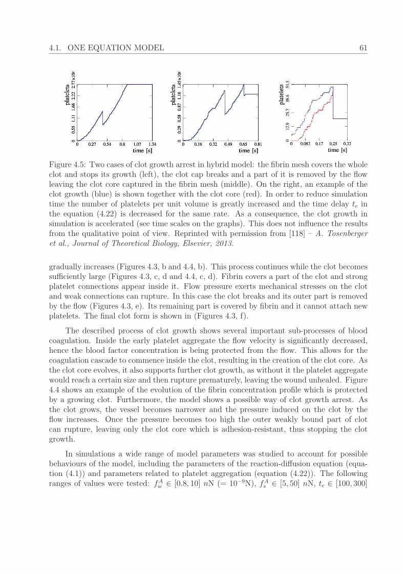
4.1. ONE EQUATION MODEL 61
Figure 4.5: Two cases of clot growth arrest in hybrid model: the fibrin mesh covers the wholeclot and stops its growth (left), the clot cap breaks and a part of it is removed by the flowleaving the clot core captured in the fibrin mesh (middle). On the right, an example of theclot growth (blue) is shown together with the clot core (red). In order to reduce simulationtime the number of platelets per unit volume is greatly increased and the time delay tc inthe equation (4.22) is decreased for the same rate. As a consequence, the clot growth insimulation is accelerated (see time scales on the graphs). This does not influence the resultsfrom the qualitative point of view. Reprinted with permission from [118] – A. Tosenbergeret al., Journal of Theoretical Biology, Elsevier, 2013.
gradually increases (Figures 4.3, b and 4.4, b). This process continues while the clot becomessufficiently large (Figures 4.3, c, d and 4.4, c, d). Fibrin covers a part of the clot and strongplatelet connections appear inside it. Flow pressure exerts mechanical stresses on the clotand weak connections can rupture. In this case the clot breaks and its outer part is removedby the flow (Figures 4.3, e). Its remaining part is covered by fibrin and it cannot attach newplatelets. The final clot form is shown in (Figures 4.3, f).
The described process of clot growth shows several important sub-processes of bloodcoagulation. Inside the early platelet aggregate the flow velocity is significantly decreased,hence the blood factor concentration is being protected from the flow. This allows for thecoagulation cascade to commence inside the clot, resulting in the creation of the clot core. Asthe clot core evolves, it also supports further clot growth, as without it the platelet aggregatewould reach a certain size and then rupture prematurely, leaving the wound unhealed. Figure4.4 shows an example of the evolution of the fibrin concentration profile which is protectedby a growing clot. Furthermore, the model shows a possible way of clot growth arrest. Asthe clot grows, the vessel becomes narrower and the pressure induced on the clot by theflow increases. Once the pressure becomes too high the outer weakly bound part of clotcan rupture, leaving only the clot core which is adhesion-resistant, thus stopping the clotgrowth.
In simulations a wide range of model parameters was studied to account for possiblebehaviours of the model, including the parameters of the reaction-diffusion equation (equa-tion (4.1)) and parameters related to platelet aggregation (equation (4.22)). The followingranges of values were tested: fAw ∈ [0.8, 10] nN (= 10−9N), fAs ∈ [5, 50] nN, tc ∈ [100, 300]

62 4.1. ONE EQUATION MODEL
Figure 4.6: Experimental results from Falati et al. (2002) [43]: on the left, platelets (red)and fibrin (green) and their co-localization (yellow) in a forming clot (flow direction is fromtop to bottom); on the right, the time course of incorporation of platelets (A) and fibrin (B)into arterial thrombi for three separate cases (denoted by 1,2,3). Reprinted and adapted bypermission from Macmillan Publishers Ltd: Nature Medicine (Falati et al., Nature Medicine8: 1175 - 1180, 2002), c© (2002).
ms, α ∈ [0.006, 0.06] mm2/min, β ∈ [0.0006, 0.042] mm2/min, uc ∈ [0.1, 0.9]. The valuesof the parameters related to inter-platelet bonds (fAw , f
As , tc) are close to the values ob-
served in a study by Pivkin et al. [98]. As protein regulatory network is approximatedby a single reaction-diffusion-advection equation, its parameters are not directly related toexperimentally observed values.
However, taking into account the time scaling explained in Section 3.1.2 (increasedplatelet density and reduced tc), the values of diffusion coefficient α used in simulations areclose to the data in [75, 84].
Depending on the choice of parameters, several clot growth patterns can be obtained.In the first case, when the diffusion coefficient is too large and the reaction coefficient istoo small, the concentration can be removed by the flow before the clot starts growing andprotects the concentration. The second regime is when the concentration production anddiffusion rates are such that fibrin gradually covers the clot, but it is slower than the clotgrowth. In that case, when the clot becomes too large to sustain the pressure from theflow, the cap of the clot breaks, leaving the core of the clot covered with fibrin, which stopsfurther clot growth (Figure 4.5 middle). In the third case, when the rates of concentrationproduction and propagation in the flow are high, the clot grows without rupture until it iscompletely covered by fibrin (Figure 4.5 left). The graph on the right side of Figure 4.5shows the growth of the clot and the clot core in time. The clot growth (excluding the clotgrowth initiation and stop stages) is almost linear, while the clot core grows approximativelyat the same rate as the clot itself. This is also observed in the experimental results obtainedby Falati et al. [43] shown in Figure 4.6 (right). Figure 4.6 (left) shows that, while the clotgrows, the formation of fibrin happens inside the clot, and it is protected by the aggregatedplatelets.
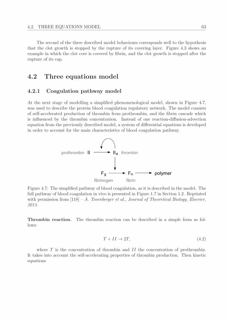
4.2. THREE EQUATIONS MODEL 63
The second of the three described model behaviours corresponds well to the hypothesisthat the clot growth is stopped by the rupture of its covering layer. Figure 4.3 shows anexample in which the clot core is covered by fibrin, and the clot growth is stopped after therupture of its cap.
4.2 Three equations model
4.2.1 Coagulation pathway model
At the next stage of modelling a simplified phenomenological model, shown in Figure 4.7,was used to describe the protein blood coagulation regulatory network. The model consistsof self-accelerated production of thrombin from prothrombin, and the fibrin cascade whichis influenced by the thrombin concentration. Instead of one reaction-diffusion-advectionequation from the previously described model, a system of differential equations is developedin order to account for the main characteristics of blood coagulation pathway.
Figure 4.7: The simplified pathway of blood coagulation, as it is described in the model. Thefull pathway of blood coagulation in vivo is presented in Figure 1.7 in Section 1.2. Reprintedwith permission from [118] – A. Tosenberger et al., Journal of Theoretical Biology, Elsevier,2013.
Thrombin reaction. The thrombin reaction can be described in a simple form as fol-lows:
T + II → 2T, (4.2)
where T is the concentration of thrombin and II the concentration of prothrombin.It takes into account the self-accelerating properties of thrombin production. Then kineticequations
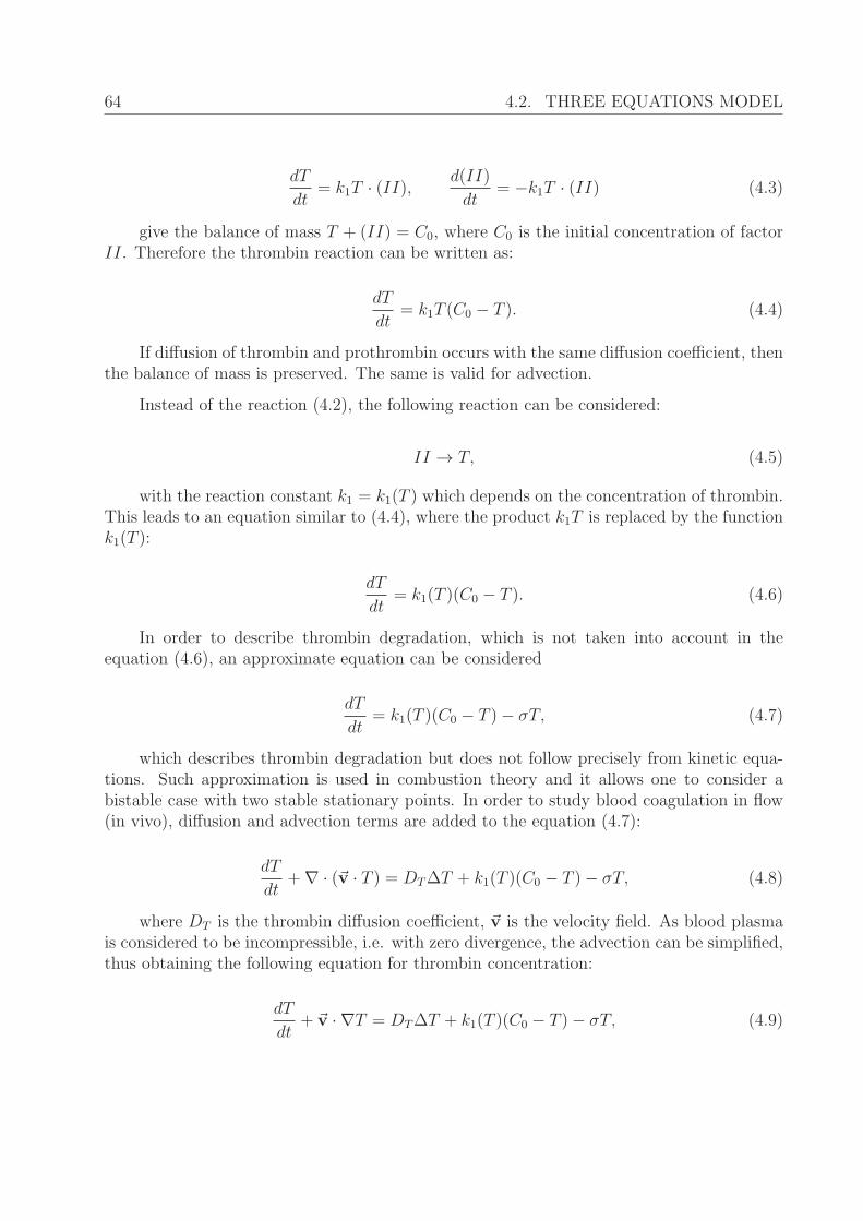
64 4.2. THREE EQUATIONS MODEL
dT
dt= k1T · (II), d(II)
dt= −k1T · (II) (4.3)
give the balance of mass T + (II) = C0, where C0 is the initial concentration of factorII. Therefore the thrombin reaction can be written as:
dT
dt= k1T (C0 − T ). (4.4)
If diffusion of thrombin and prothrombin occurs with the same diffusion coefficient, thenthe balance of mass is preserved. The same is valid for advection.
Instead of the reaction (4.2), the following reaction can be considered:
II → T, (4.5)
with the reaction constant k1 = k1(T ) which depends on the concentration of thrombin.This leads to an equation similar to (4.4), where the product k1T is replaced by the functionk1(T ):
dT
dt= k1(T )(C0 − T ). (4.6)
In order to describe thrombin degradation, which is not taken into account in theequation (4.6), an approximate equation can be considered
dT
dt= k1(T )(C0 − T )− σT, (4.7)
which describes thrombin degradation but does not follow precisely from kinetic equa-tions. Such approximation is used in combustion theory and it allows one to consider abistable case with two stable stationary points. In order to study blood coagulation in flow(in vivo), diffusion and advection terms are added to the equation (4.7):
dT
dt+∇ · (�v · T ) = DTΔT + k1(T )(C0 − T )− σT, (4.8)
where DT is the thrombin diffusion coefficient, �v is the velocity field. As blood plasmais considered to be incompressible, i.e. with zero divergence, the advection can be simplified,thus obtaining the following equation for thrombin concentration:
dT
dt+ �v · ∇T = DTΔT + k1(T )(C0 − T )− σT, (4.9)
4.2. THREE EQUATIONS MODEL 65
Fibrin reactions. Consider, next, the reactions
Fg → Fn → Fp, (4.10)
where Fp is fibrin polymer. Unlike thrombin which is produced locally at the injurysite and inside the the clot, fibrinogen is synthesized in the liver and constantly circulates inthe blood stream. The availability of thrombin, as an enzyme, is necessary to produce fibrinfrom fibrinogen. Therefore, it is important to take into account the flow influence on bothconcentrations - thrombin and fibrinogen. We omit fibrin in the reaction scheme (4.10) andconsider instead a simplified reaction Fg → Fp. Then, the reaction can be represented bythe following model:
∂Fg∂t
+ �v · ∇Fg = DFgΔFg − k3(T )Fg, (4.11)
∂Fp∂t
= k3(T )Fg, (4.12)
whereDFg is the fibrinogen diffusion coefficient, and k3(T ) is the reaction constant whichdepends on the concentration of thrombin. The equation (4.11) describes fibrinogen diffusionin flow, and the equation (4.12) describes the concentration of fibrin polymers which forman insoluble network and thus do not diffuse or flow.
Coagulation pathway model. By combining the equation(4.9) for thrombin concen-tration, and equations (4.11) and (4.12) for fibrinogen and fibrin polymer concentrationsrespectively, one obtains the following model:
dT
dt+ �v · ∇T = DTΔT + k1(T )(C0 − T )− σT,
∂Fg∂t
+ �v · ∇Fg = DFgΔFg − k3(T )Fg, (4.13)
∂Fp∂t
= k3(T )Fg.
In order to model the self-amplifying thrombin reaction, the reaction function k1(T ) isdefined as follows:
k1(T ) = k01
T 2
T0 + T, (4.14)
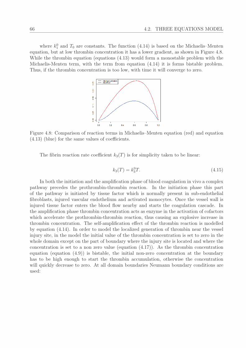
66 4.2. THREE EQUATIONS MODEL
where k01 and T0 are constants. The function (4.14) is based on the Michaelis–Menten
equation, but at low thrombin concentration it has a lower gradient, as shown in Figure 4.8.While the thrombin equation (equations (4.13) would form a monostable problem with theMichaelis-Menten term, with the term from equation (4.14) it is forms bistable problem.Thus, if the thrombin concentration is too low, with time it will converge to zero.
Figure 4.8: Comparison of reaction terms in Michaelis–Menten equation (red) and equation(4.13) (blue) for the same values of coefficients.
The fibrin reaction rate coefficient k3(T ) is for simplicity taken to be linear:
k3(T ) = k03T. (4.15)
In both the initiation and the amplification phase of blood coagulation in vivo a complexpathway precedes the prothrombin-thrombin reaction. In the initiation phase this partof the pathway is initiated by tissue factor which is normally present in sub-endothelialfibroblasts, injured vascular endothelium and activated monocytes. Once the vessel wall isinjured tissue factor enters the blood flow nearby and starts the coagulation cascade. Inthe amplification phase thrombin concentration acts as enzyme in the activation of cofactorswhich accelerate the prothrombin-thrombin reaction, thus causing an explosive increase inthrombin concentration. The self-amplification effect of the thrombin reaction is modelledby equation (4.14). In order to model the localized generation of thrombin near the vesselinjury site, in the model the initial value of the thrombin concentration is set to zero in thewhole domain except on the part of boundary where the injury site is located and where theconcentration is set to a non zero value (equation (4.17)). As the thrombin concentrationequation (equation (4.9)) is bistable, the initial non-zero concentration at the boundaryhas to be high enough to start the thrombin accumulation, otherwise the concentrationwill quickly decrease to zero. At all domain boundaries Neumann boundary conditions areused:
4.2. THREE EQUATIONS MODEL 67
∂T
∂x
∣∣x=0,L
=∂T
∂y
∣∣y=0,D
= 0 (4.16)
T (x, y, t)∣∣t=0
=
⎧⎨⎩1, if x ∈ [wB, wE] and y = 0,
0, if x /∈ [wB, wE] or y = 0,(4.17)
where [0, L] × [0, D] is the simulation domain, i.e. a part of blood vessel of the lengthL and diameter D, and where [wB, wE] × {0} is the part of domain representing the vesselinjury site.
The primary function of thrombin is the conversion of fibrinogen to fibrin. Fibrinogen,being synthesised in the liver by hepatocytes, is constantly present in a healthy bloodstream.Therefore, in the model, the initial concentration of fibrinogen is set to some value F 0
g in thewhole domain and at the inflow boundary Dirichlet boundary conditions are used, while theremaining boundaries are described with zero Neumann boundary conditions:
∂Fg∂x
∣∣x=L
=∂Fg∂y
∣∣y=0,D
= 0, (4.18)
Fg∣∣x=0
= F 0g , (4.19)
Fg(x, y, t)∣∣t=0
= F 0g . (4.20)
4.2.2 Platelet aggregation
The first hybrid model described only two levels of inter-platelet bonding strengths – theweaker adhesion bond and the stronger bond between activated platelets. In the secondhybrid model the fibrin polymer concentration is introduced. To describe the effects of thefibrin net on the aggregated platelets two new conditions are added. The first one is theadhesion resistance effect present in platelets that are coated in fibrin polymers. Instead ofthe critical concentration constant uc used in the first hybrid model, a similar constant cFg
is introduced. cFg denotes the critical fibrin polymer (Fp) concentration, above which it isconsidered that the fibrin net has been formed. Hence, platelets that are considered to becovered by the fibrin net become adhesion resistant. The second effect of the fibrin net isthat it reinforces the platelet aggregate. Therefore, a third level of strength of inter-plateletbonds is introduced in the model describing the aggregated platelets covered by the fibrinnet. Following the description, the adhesion force is modelled as a pairwise force betweentwo platelets expressed in the form of Hooke’s law:
68 4.2. THREE EQUATIONS MODEL
FAij = fA(tij)
(1− rij
dC
)rij, (4.21)
where fA is the force strength coefficient and dC is the force relaxation distance which isequal to two times the physical radius of the platelets. As platelet binding occurs due totheir surface adhesion receptors, two platelets in a flow connect when they come in physicalcontact, i.e. rij ≤ dC (connection criterium). Platelets remain connected until their distancedoes not exceed a critical value dD (disconnection criterium) which is greater than dC . Weset dD equal to 1.3 times of the platelet diameter. The force strength coefficient fA inequation (4.21) is modelled in the following way to describe three strengths of inter-plateletbonds:
fA(tij) =
⎧⎪⎪⎪⎪⎪⎨⎪⎪⎪⎪⎪⎩fA1 if Fp(i) or Fp(j) < cFp , and tij < tc,
fA2 if Fp(i) or Fp(j) < cFp , and tij ≥ tc,
fA3 if Fp(i) and Fp(j) ≥ cFp ,
(4.22)
where fA1 < fA2 < fA3 are the three strengths of inter-platelet connections, representingrespectively a weak bond due to GPIb receptors, a medium bond due to platelet activationand a strong bond due to the reinforcement by the fibrin polymer net. tc is the time neededfor platelet activation measured from the moment when the connection is established. Asthe platelet activation process is not at the focus of this study at the moment, the activationperiod serves as a basic approximation of the platelet activation process due to the contactand proximity of other activated platelets. Fp(i) and Fp(j) are levels of fibrin polymer Fp atpositions of particles i and j respectively. cFp is the critical level of fibrin polymer. A plateletis considered to be a part of the clot core if it is in the clot and the fibrin concentration hasbeen larger than cFp at the position of that platelet. Therefore, the clot core is a part of theclot covered by a concentration of Fp larger than cFp . As the platelets that are coated withfibrin are adhesion resistant, the same condition is applied in the model on the platelets in thecore which cannot establish new bonds. In the case of physical contact between two plateletsthat are not connected, one of which is non-adhesive, an additional repulsing force has to beintroduced between them in order to prevent them from occupying the same space.
4.2.3 Parameters
A typical clot structure is shown in Figure 4.9. There are three types of platelet connections,weak (light red lines between their centres), medium (dark red lines) and strong (blacklines). Medium connections appear if platelets are weakly connected during the time periodtc. Hence we model the platelet activation and emergence of medium connections as a time
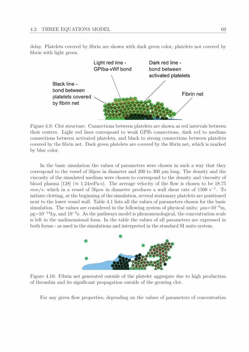
4.2. THREE EQUATIONS MODEL 69
delay. Platelets covered by fibrin are shown with dark green color, platelets not covered byfibrin with light green.
Figure 4.9: Clot structure. Connections between platelets are shown as red intervals betweentheir centres. Light red lines correspond to weak GPIb connections, dark red to mediumconnections between activated platelets, and black to strong connections between plateletscovered by the fibrin net. Dark green platelets are covered by the fibrin net, which is markedby blue color.
In the basic simulation the values of parameters were chosen in such a way that theycorrespond to the vessel of 50μm in diameter and 200 to 300 μm long. The density and theviscosity of the simulated medium were chosen to correspond to the density and viscosity ofblood plasma [128] (≈ 1.24mPa·s). The average velocity of the flow is chosen to be 18.75mm/s, which in a vessel of 50μm in diameter produces a wall shear rate of 1500 s−1. Toinitiate clotting, at the beginning of the simulation, several stationary platelets are positionednext to the lower vessel wall. Table 4.1 lists all the values of parameters chosen for the basicsimulation. The values are considered in the following system of physical units: μm=10−6m,pg=10−14kg, and 10−2s. As the pathways model is phenomenological, the concentration scaleis left in the undimensional form. In the table the values of all parameters are expressed inboth forms - as used in the simulations and interpreted in the standard SI units system.
Figure 4.10: Fibrin net generated outside of the platelet aggregate due to high productionof thrombin and its significant propagation outside of the growing clot.
For any given flow properties, depending on the values of parameters of concentration
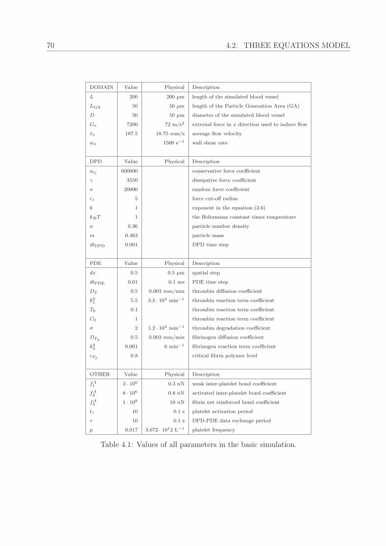
70 4.2. THREE EQUATIONS MODEL
DOMAIN Value Physical Description
L 200 200 μm length of the simulated blood vessel
LGA 50 50 μm length of the Particle Generation Area (GA)
D 50 50 μm diameter of the simulated blood vessel
Gx 7200 72 m/s2 external force in x direction used to induce flow
vx 187.5 18.75 mm/s average flow velocity
wx 1500 s−1 wall shear rate
DPD Value Physical Description
aij 600000 conservative force coefficient
γ 3550 dissipative force coefficient
σ 20000 random force coefficient
rc 5 force cut-off radius
k 1 exponent in the equation (2.6)
kBT 1 the Boltzmann constant times temperature
n 0.36 particle number density
m 0.463 particle mass
dtDPD 0.001 DPD time step
PDE Value Physical Description
dx 0.5 0.5 μm spatial step
dtPDE 0.01 0.1 ms PDE time step
DT 0.5 0.003 mm/min thrombin diffusion coefficient
k01 5.5 3.3 · 104 min−1 thrombin reaction term coefficient
T0 0.1 thrombin reaction term coefficient
C0 1 thrombin reaction term coefficient
σ 2 1.2 · 104 min−1 thrombin degradation coefficient
DFg 0.5 0.003 mm/min fibrinogen diffusion coefficient
k03 0.001 6 min−1 fibrinogen reaction term coefficient
cFp 0.8 critical fibrin polymer level
OTHER Value Physical Description
fA1 3 · 106 0.3 nN weak inter-platelet bond coefficient
fA2 8 · 106 0.8 nN activated inter-platelet bond coefficient
fA3 1 · 108 10 nN fibrin net reinforced bond coefficient
tc 10 0.1 s platelet activation period
τ 10 0.1 s DPD-PDE data exchange period
p 0.017 3.672 · 1012 L−1 platelet frequency
Table 4.1: Values of all parameters in the basic simulation.
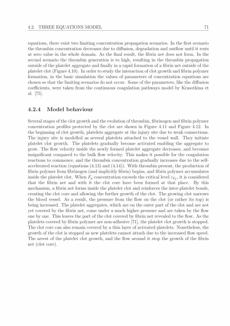
4.2. THREE EQUATIONS MODEL 71
equations, there exist two limiting concentration propagation scenarios. In the first scenariothe thrombin concentration decreases due to diffusion, degradation and outflow until it restsat zero value in the whole domain. As the final result, the fibrin net does not form. In thesecond scenario the thrombin generation is to high, resulting in the thrombin propagationoutside of the platelet aggregate and finally in a rapid formation of a fibrin net outside of theplatelet clot (Figure 4.10). In order to study the interaction of clot growth and fibrin polymerformation, in the basic simulation the values of parameters of concentration equations arechosen so that the limiting scenarios do not occur. Some of the parameters, like the diffusioncoefficients, were taken from the continuous coagulation pathways model by Krasotkina etal. [75].
4.2.4 Model behaviour
Several stages of the clot growth and the evolution of thrombin, fibrinogen and fibrin polymerconcentration profiles protected by the clot are shown in Figure 4.11 and Figure 4.12. Inthe beginning of clot growth, platelets aggregate at the injury site due to weak connections.The injury site is modelled as several platelets attached to the vessel wall. They initiateplatelet clot growth. The platelets gradually become activated enabling the aggregate togrow. The flow velocity inside the newly formed platelet aggregate decreases, and becomesinsignificant compared to the bulk flow velocity. This makes it possible for the coagulationreactions to commence, and the thrombin concentration gradually increases due to the self-accelerated reaction (equations (4.13) and (4.14)). With thrombin present, the production offibrin polymer from fibrinogen (and implicitly fibrin) begins, and fibrin polymer accumulatesinside the platelet clot. When Fp concentration exceeds the critical level cFp , it is consideredthat the fibrin net and with it the clot core have been formed at that place. By thismechanism, a fibrin net forms inside the platelet clot and reinforces the inter-platelet bonds,creating the clot core and allowing the further growth of the clot. The growing clot narrowsthe blood vessel. As a result, the pressure from the flow on the clot (or rather its top) isbeing increased. The platelet aggregates, which are on the outer part of the clot and are notyet covered by the fibrin net, come under a much higher pressure and are taken by the flowone by one. This leaves the part of the clot covered by fibrin net revealed to the flow. As theplatelets covered by fibrin polymer are non-adhesive [71], the platelet clot growth is stopped.The clot core can also remain covered by a thin layer of activated platelets. Nonetheless, thegrowth of the clot is stopped as new platelets cannot attach due to the increased flow speed.The arrest of the platelet clot growth, and the flow around it stop the growth of the fibrinnet (clot core).
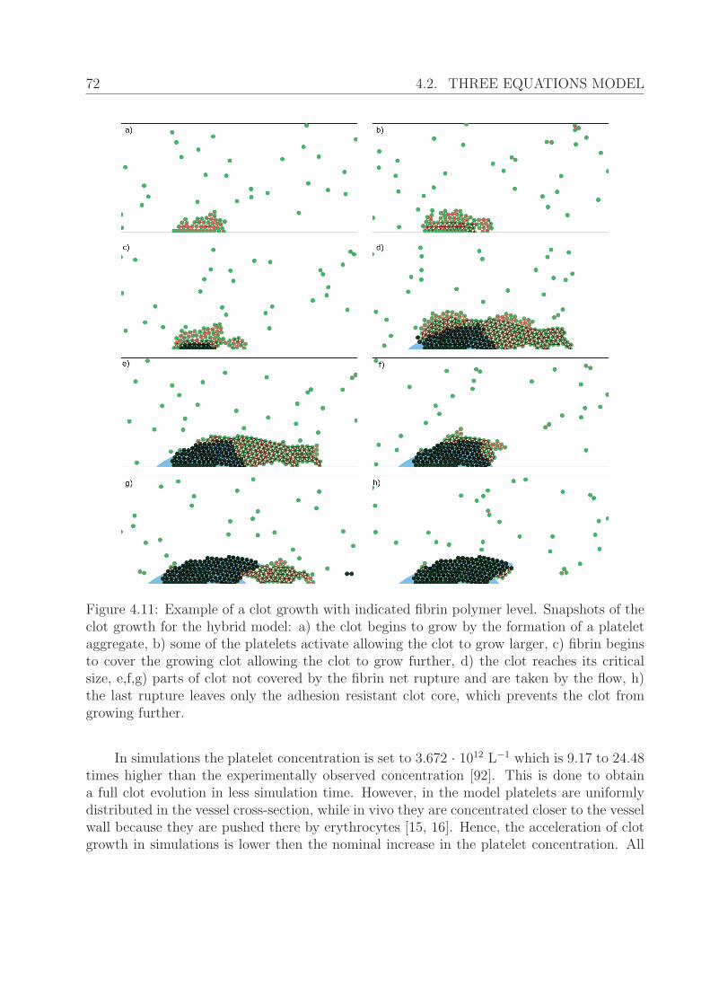
72 4.2. THREE EQUATIONS MODEL
Figure 4.11: Example of a clot growth with indicated fibrin polymer level. Snapshots of theclot growth for the hybrid model: a) the clot begins to grow by the formation of a plateletaggregate, b) some of the platelets activate allowing the clot to grow larger, c) fibrin beginsto cover the growing clot allowing the clot to grow further, d) the clot reaches its criticalsize, e,f,g) parts of clot not covered by the fibrin net rupture and are taken by the flow, h)the last rupture leaves only the adhesion resistant clot core, which prevents the clot fromgrowing further.
In simulations the platelet concentration is set to 3.672 · 1012 L−1 which is 9.17 to 24.48times higher than the experimentally observed concentration [92]. This is done to obtaina full clot evolution in less simulation time. However, in the model platelets are uniformlydistributed in the vessel cross-section, while in vivo they are concentrated closer to the vesselwall because they are pushed there by erythrocytes [15, 16]. Hence, the acceleration of clotgrowth in simulations is lower then the nominal increase in the platelet concentration. All
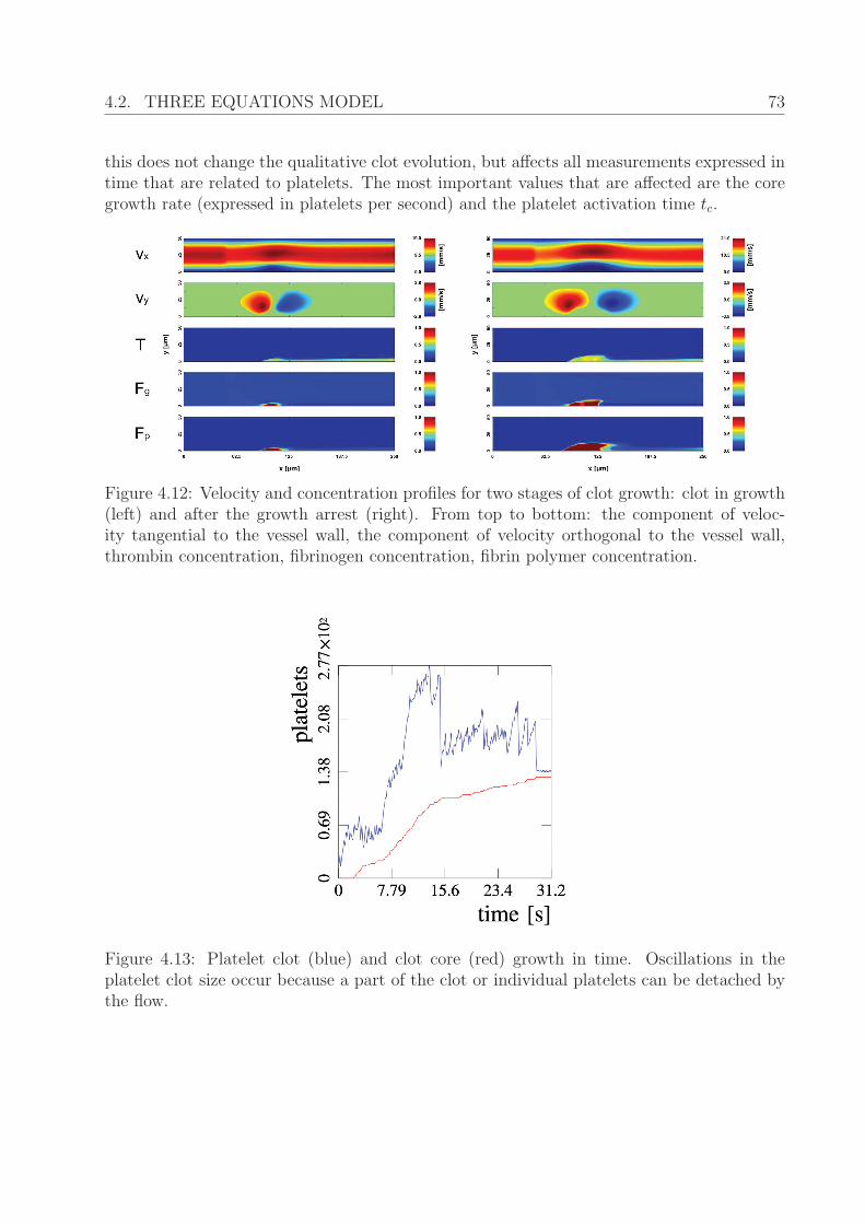
4.2. THREE EQUATIONS MODEL 73
this does not change the qualitative clot evolution, but affects all measurements expressed intime that are related to platelets. The most important values that are affected are the coregrowth rate (expressed in platelets per second) and the platelet activation time tc.
Figure 4.12: Velocity and concentration profiles for two stages of clot growth: clot in growth(left) and after the growth arrest (right). From top to bottom: the component of veloc-ity tangential to the vessel wall, the component of velocity orthogonal to the vessel wall,thrombin concentration, fibrinogen concentration, fibrin polymer concentration.
Figure 4.13: Platelet clot (blue) and clot core (red) growth in time. Oscillations in theplatelet clot size occur because a part of the clot or individual platelets can be detached bythe flow.
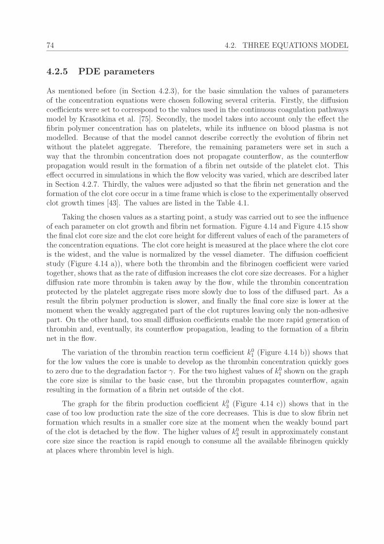
74 4.2. THREE EQUATIONS MODEL
4.2.5 PDE parameters
As mentioned before (in Section 4.2.3), for the basic simulation the values of parametersof the concentration equations were chosen following several criteria. Firstly, the diffusioncoefficients were set to correspond to the values used in the continuous coagulation pathwaysmodel by Krasotkina et al. [75]. Secondly, the model takes into account only the effect thefibrin polymer concentration has on platelets, while its influence on blood plasma is notmodelled. Because of that the model cannot describe correctly the evolution of fibrin netwithout the platelet aggregate. Therefore, the remaining parameters were set in such away that the thrombin concentration does not propagate counterflow, as the counterflowpropagation would result in the formation of a fibrin net outside of the platelet clot. Thiseffect occurred in simulations in which the flow velocity was varied, which are described laterin Section 4.2.7. Thirdly, the values were adjusted so that the fibrin net generation and theformation of the clot core occur in a time frame which is close to the experimentally observedclot growth times [43]. The values are listed in the Table 4.1.
Taking the chosen values as a starting point, a study was carried out to see the influenceof each parameter on clot growth and fibrin net formation. Figure 4.14 and Figure 4.15 showthe final clot core size and the clot core height for different values of each of the parameters ofthe concentration equations. The clot core height is measured at the place where the clot coreis the widest, and the value is normalized by the vessel diameter. The diffusion coefficientstudy (Figure 4.14 a)), where both the thrombin and the fibrinogen coefficient were variedtogether, shows that as the rate of diffusion increases the clot core size decreases. For a higherdiffusion rate more thrombin is taken away by the flow, while the thrombin concentrationprotected by the platelet aggregate rises more slowly due to loss of the diffused part. As aresult the fibrin polymer production is slower, and finally the final core size is lower at themoment when the weakly aggregated part of the clot ruptures leaving only the non-adhesivepart. On the other hand, too small diffusion coefficients enable the more rapid generation ofthrombin and, eventually, its counterflow propagation, leading to the formation of a fibrinnet in the flow.
The variation of the thrombin reaction term coefficient k01 (Figure 4.14 b)) shows that
for the low values the core is unable to develop as the thrombin concentration quickly goesto zero due to the degradation factor γ. For the two highest values of k0
1 shown on the graphthe core size is similar to the basic case, but the thrombin propagates counterflow, againresulting in the formation of a fibrin net outside of the clot.
The graph for the fibrin production coefficient k03 (Figure 4.14 c)) shows that in the
case of too low production rate the size of the core decreases. This is due to slow fibrin netformation which results in a smaller core size at the moment when the weakly bound partof the clot is detached by the flow. The higher values of k0
3 result in approximately constantcore size since the reaction is rapid enough to consume all the available fibrinogen quicklyat places where thrombin level is high.
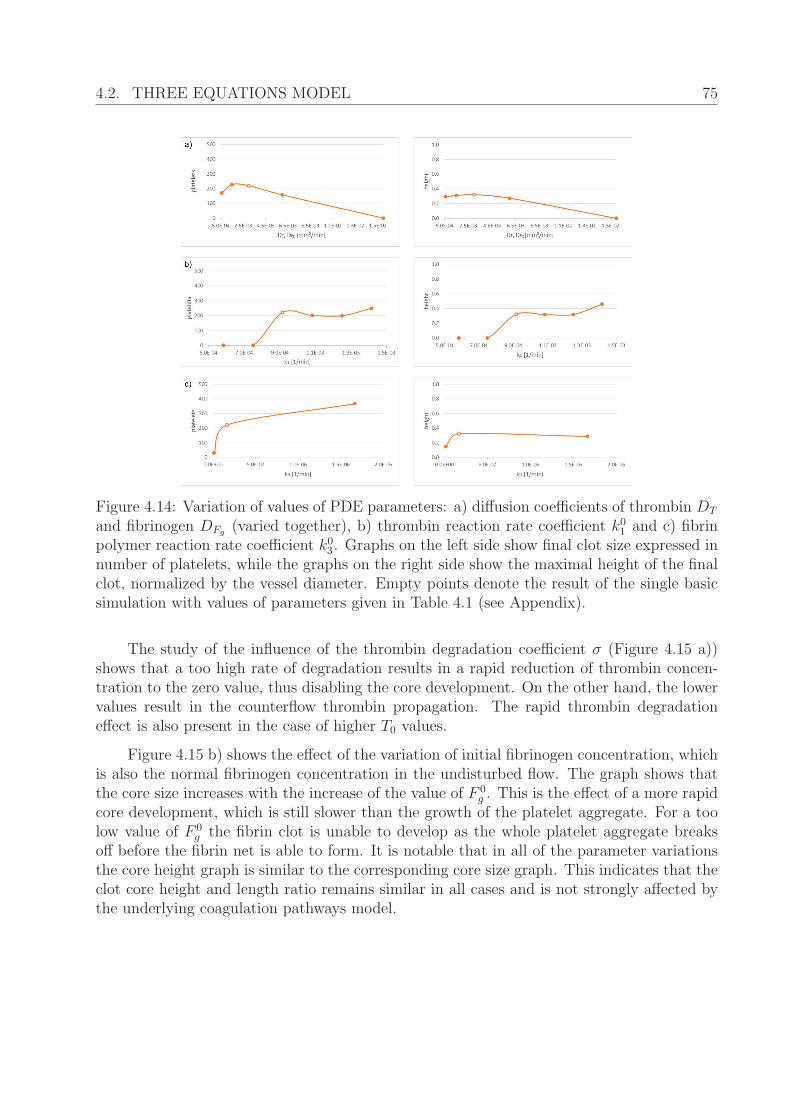
4.2. THREE EQUATIONS MODEL 75
Figure 4.14: Variation of values of PDE parameters: a) diffusion coefficients of thrombin DT
and fibrinogen DFg (varied together), b) thrombin reaction rate coefficient k01 and c) fibrin
polymer reaction rate coefficient k03. Graphs on the left side show final clot size expressed in
number of platelets, while the graphs on the right side show the maximal height of the finalclot, normalized by the vessel diameter. Empty points denote the result of the single basicsimulation with values of parameters given in Table 4.1 (see Appendix).
The study of the influence of the thrombin degradation coefficient σ (Figure 4.15 a))shows that a too high rate of degradation results in a rapid reduction of thrombin concen-tration to the zero value, thus disabling the core development. On the other hand, the lowervalues result in the counterflow thrombin propagation. The rapid thrombin degradationeffect is also present in the case of higher T0 values.
Figure 4.15 b) shows the effect of the variation of initial fibrinogen concentration, whichis also the normal fibrinogen concentration in the undisturbed flow. The graph shows thatthe core size increases with the increase of the value of F 0
g . This is the effect of a more rapidcore development, which is still slower than the growth of the platelet aggregate. For a toolow value of F 0
g the fibrin clot is unable to develop as the whole platelet aggregate breaksoff before the fibrin net is able to form. It is notable that in all of the parameter variationsthe core height graph is similar to the corresponding core size graph. This indicates that theclot core height and length ratio remains similar in all cases and is not strongly affected bythe underlying coagulation pathways model.
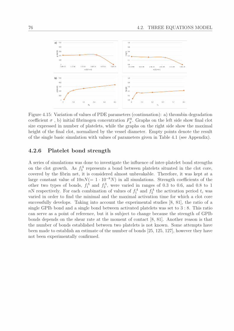
76 4.2. THREE EQUATIONS MODEL
Figure 4.15: Variation of values of PDE parameters (continuation): a) thrombin degradationcoefficient σ , b) initial fibrinogen concentration F 0
g . Graphs on the left side show final clotsize expressed in number of platelets, while the graphs on the right side show the maximalheight of the final clot, normalized by the vessel diameter. Empty points denote the resultof the single basic simulation with values of parameters given in Table 4.1 (see Appendix).
4.2.6 Platelet bond strength
A series of simulations was done to investigate the influence of inter-platelet bond strengthson the clot growth. As fA3 represents a bond between platelets situated in the clot core,covered by the fibrin net, it is considered almost unbreakable. Therefore, it was kept at alarge constant value of 10nN(= 1 · 10−8N) in all simulations. Strength coefficients of theother two types of bonds, fA1 and fA2 , were varied in ranges of 0.3 to 0.6, and 0.8 to 1nN respectively. For each combination of values of fA1 and fA2 the activation period tc wasvaried in order to find the minimal and the maximal activation time for which a clot coresuccessfully develops. Taking into account the experimental studies [8, 81], the ratio of asingle GPIb bond and a single bond between activated platelets was set to 3 : 8. This ratiocan serve as a point of reference, but it is subject to change because the strength of GPIbbonds depends on the shear rate at the moment of contact [8, 81]. Another reason is thatthe number of bonds established between two platelets is not known. Some attempts havebeen made to establish an estimate of the number of bonds [25, 125, 127], however they havenot been experimentally confirmed.
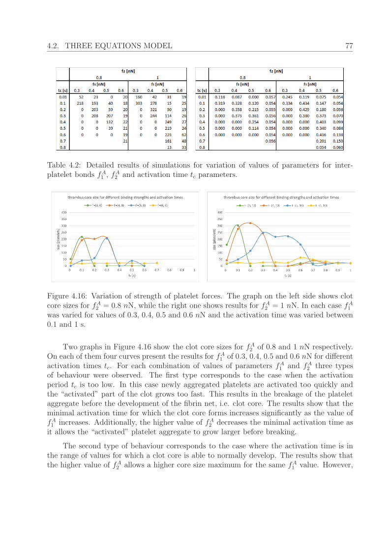
4.2. THREE EQUATIONS MODEL 77
Table 4.2: Detailed results of simulations for variation of values of parameters for inter-platelet bonds fA1 , f
A2 and activation time tc parameters.
Figure 4.16: Variation of strength of platelet forces. The graph on the left side shows clotcore sizes for fA2 = 0.8 nN, while the right one shows results for fA2 = 1 nN. In each case fA1was varied for values of 0.3, 0.4, 0.5 and 0.6 nN and the activation time was varied between0.1 and 1 s.
Two graphs in Figure 4.16 show the clot core sizes for fA2 of 0.8 and 1 nN respectively.On each of them four curves present the results for fA1 of 0.3, 0.4, 0.5 and 0.6 nN for differentactivation times tc. For each combination of values of parameters fA1 and fA2 three typesof behaviour were observed. The first type corresponds to the case when the activationperiod tc is too low. In this case newly aggregated platelets are activated too quickly andthe “activated” part of the clot grows too fast. This results in the breakage of the plateletaggregate before the development of the fibrin net, i.e. clot core. The results show that theminimal activation time for which the clot core forms increases significantly as the value offA1 increases. Additionally, the higher value of fA2 decreases the minimal activation time asit allows the “activated” platelet aggregate to grow larger before breaking.
The second type of behaviour corresponds to the case where the activation time is inthe range of values for which a clot core is able to normally develop. The results show thatthe higher value of fA2 allows a higher core size maximum for the same fA1 value. However,

78 4.2. THREE EQUATIONS MODEL
maxima for the different values of fA2 are not achieved for the same activation times.
Figure 4.17: Clot core growth in first 40 s for values of fA1 and fA2 of 0.5 and 1 nN respectively.Each graph corresponds to a different value of activation time tc - from 0.01 to 0.7 seconds.
The third type of behaviour occurs when the activation time is too long, which preventsthe formation of the clot core. As the activation time is too long, the weakly bound plateletaggregates grow to quickly and they break off before any consisting platelets can activate.Hence no activation occurs, and the clot cannot sustain flow pressure.
Figure 4.17 shows clot core growth in first 40 seconds for fA1 = 0.4 nN, fA2 = 1 nN,and activation times from 0.01 to 0.7 seconds. For values of the activation time 0.01 and 0.7seconds the clot was unable to develop. In the case of a too rapid activation, as the adheringplatelets activate immediately after the adhesion, the platelet aggregate rapidly grows andbreaks off while clot core is still too small. In the case of the long activation time, aggregatedplatelets cannot sustain the increase of the flow shear rate at the surface of the growing clot,and thus do not get activated, leaving again an underdeveloped core. Generally speaking, ashorter activation time will have for an effect a faster growth of the platelet aggregate. Thegrowth rate of the fibrin net is bounded by the growth rate of the platelet aggregate, butalso by the values of parameters of the system (4.13). Thus, when the platelet aggregategrowth is too rapid the fibrin net growth rate becomes bounded by the underlying regulatorynetwork, and the weaker parts of the clot break-off sooner, leaving the smaller core. This
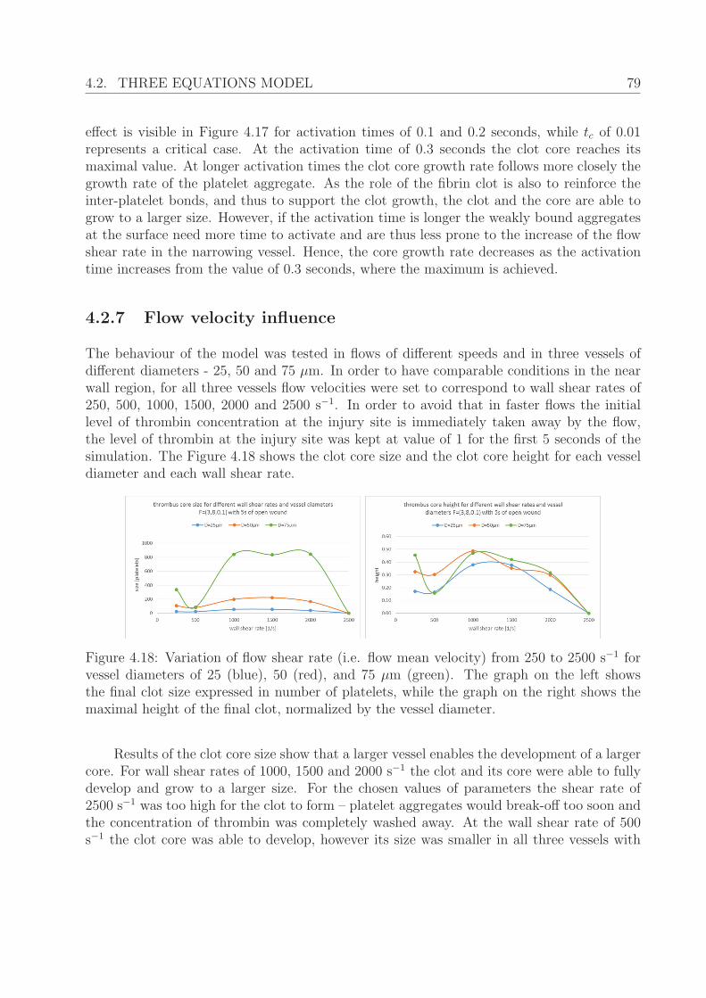
4.2. THREE EQUATIONS MODEL 79
effect is visible in Figure 4.17 for activation times of 0.1 and 0.2 seconds, while tc of 0.01represents a critical case. At the activation time of 0.3 seconds the clot core reaches itsmaximal value. At longer activation times the clot core growth rate follows more closely thegrowth rate of the platelet aggregate. As the role of the fibrin clot is also to reinforce theinter-platelet bonds, and thus to support the clot growth, the clot and the core are able togrow to a larger size. However, if the activation time is longer the weakly bound aggregatesat the surface need more time to activate and are thus less prone to the increase of the flowshear rate in the narrowing vessel. Hence, the core growth rate decreases as the activationtime increases from the value of 0.3 seconds, where the maximum is achieved.
4.2.7 Flow velocity influence
The behaviour of the model was tested in flows of different speeds and in three vessels ofdifferent diameters - 25, 50 and 75 μm. In order to have comparable conditions in the nearwall region, for all three vessels flow velocities were set to correspond to wall shear rates of250, 500, 1000, 1500, 2000 and 2500 s−1. In order to avoid that in faster flows the initiallevel of thrombin concentration at the injury site is immediately taken away by the flow,the level of thrombin at the injury site was kept at value of 1 for the first 5 seconds of thesimulation. The Figure 4.18 shows the clot core size and the clot core height for each vesseldiameter and each wall shear rate.
Figure 4.18: Variation of flow shear rate (i.e. flow mean velocity) from 250 to 2500 s−1 forvessel diameters of 25 (blue), 50 (red), and 75 μm (green). The graph on the left showsthe final clot size expressed in number of platelets, while the graph on the right shows themaximal height of the final clot, normalized by the vessel diameter.
Results of the clot core size show that a larger vessel enables the development of a largercore. For wall shear rates of 1000, 1500 and 2000 s−1 the clot and its core were able to fullydevelop and grow to a larger size. For the chosen values of parameters the shear rate of2500 s−1 was too high for the clot to form – platelet aggregates would break-off too soon andthe concentration of thrombin was completely washed away. At the wall shear rate of 500s−1 the clot core was able to develop, however its size was smaller in all three vessels with
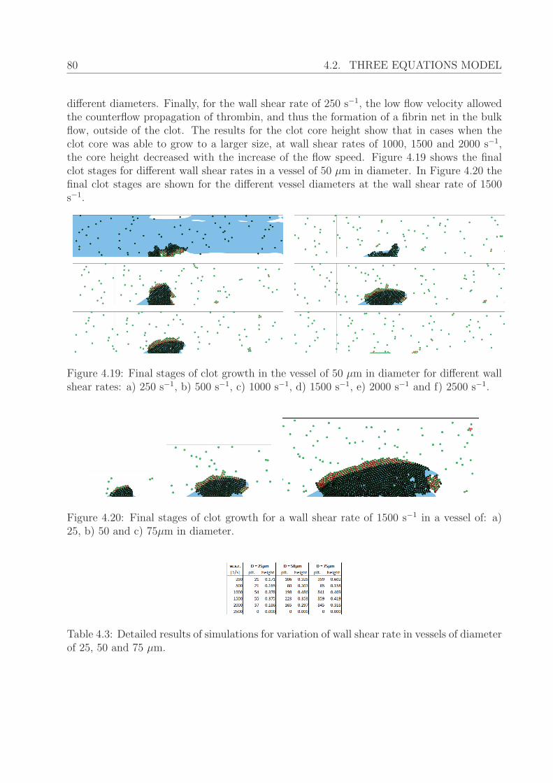
80 4.2. THREE EQUATIONS MODEL
different diameters. Finally, for the wall shear rate of 250 s−1, the low flow velocity allowedthe counterflow propagation of thrombin, and thus the formation of a fibrin net in the bulkflow, outside of the clot. The results for the clot core height show that in cases when theclot core was able to grow to a larger size, at wall shear rates of 1000, 1500 and 2000 s−1,the core height decreased with the increase of the flow speed. Figure 4.19 shows the finalclot stages for different wall shear rates in a vessel of 50 μm in diameter. In Figure 4.20 thefinal clot stages are shown for the different vessel diameters at the wall shear rate of 1500s−1.
Figure 4.19: Final stages of clot growth in the vessel of 50 μm in diameter for different wallshear rates: a) 250 s−1, b) 500 s−1, c) 1000 s−1, d) 1500 s−1, e) 2000 s−1 and f) 2500 s−1.
Figure 4.20: Final stages of clot growth for a wall shear rate of 1500 s−1 in a vessel of: a)25, b) 50 and c) 75μm in diameter.
Table 4.3: Detailed results of simulations for variation of wall shear rate in vessels of diameterof 25, 50 and 75 μm.
81
Chapter 5
Mathematical analysis of a modelproblem for atherosclerosis
5.1 Introduction
Atherosclerosis is a condition which can take several decades to develop and show firstnoticeable symptoms. For a long period of time monocytes slowly accumulate in the vesselwall intima, as a response to oxidized Low-Density Lipoprotein (LDL) molecules. Thisprocess has a twofold effect. First, the vessel wall slowly thickens as monocytes accumulatein the wall intima, which gradually narrows the lumen of the vessel. This can lead toan immune response and can start a chronic inflammation with auto-amplifying effects.Second, in a case of inflammation, the large amount of accumulated monocytes (i.e. foamcells) results in structural changes of vessel wall, so called remodelling, and developmentof the atherosclerotic plaque. Therefore, we can consider two aspects of atherosclerosisdevelopment: inflammation and vessel remodelling.
The vessel remodelling aspect of atherosclerosis is biologically closely related to bloodcoagulation. In the process of vessel wall remodelling, muscle cells proliferate and migratetowards the inner surface of the vessel wall. This results in formation of a fibrous capover the lipid deposit, so called atherosclerotic plaque. The mechanical properties of theplaque significantly differ from the properties of a healthy vessel wall. The surface of theplaque is more rigid and prone to rupture due to flow pressure and reduced surface elasticity.Structural changes together with the narrowed lumen and increased flow pressure, make thevessel wall highly susceptible to rupture, which would initiate blood coagulation on top ofthe plaque. Formation of blood clot on the already narrowed part of the vessel can leadeither to complete occlusion of the vessel or to rupture of the blood clot, both of whichusually have tragic consequences. From modelling point of view, hybrid models similar toones described in Chapter 4 can be used to model the remodelling aspect of atherosclerosis.
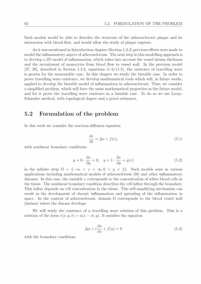
82 5.2. FORMULATION OF THE PROBLEM
Such models would be able to describe the structure of the atherosclerotic plaque and itsinteraction with blood flow, and would allow the study of plaque rupture.
As it was mentioned in Introduction chapter (Section 1.3.2) previous efforts were made tomodel the inflammatory aspect of atherosclerosis. The next step in this modelling approach isto develop a 2D model of inflammation, which takes into account the vessel intima thicknessand the recruitment of monocytes from blood flow to vessel wall. In the previous model[37, 38], described in Section 1.3.2, equations (1.4)-(1.5), the existence of travelling waveis proven for the monostable case. In this chapter we study the bistable case. In order toprove travelling wave existence, we develop mathematical tools which will, in future works,applied to develop the bistable model of inflammation in atherosclerosis. Thus, we considera simplified problem, which will have the same mathematical properties as the future model,and for it prove the travelling wave existence in a bistable case. To do so we use Leray-Schauder method, with topological degree and a priori estimates.
5.2 Formulation of the problem
In this work we consider the reaction-diffusion equation
∂v
∂t= Δv + f(v), (5.1)
with nonlinear boundary conditions:
y = 0 :∂v
∂y= 0, y = 1 :
∂v
∂y= g(v) (5.2)
in the infinite strip Ω = {−∞ < x < ∞, 0 < y < 1}. Such models arise in variousapplications including mathematical models of atherosclerosis [38] and other inflammatorydiseases. In this case, the variable v corresponds to the concentration of white blood cells inthe tissue. The nonlinear boundary condition describes the cell influx through the boundary.This influx depends on cell concentration in the tissue. This self-amplifying mechanism canresult in the development of chronic inflammation and spreading of the inflammation inspace. In the context of atherosclerosis, domain Ω corresponds to the blood vessel wall(intima) where the disease develops.
We will study the existence of a travelling wave solution of this problem. This is asolution of the form v(x, y, t) = u(x− ct, y). It satisfies the equation
Δu+ c∂u
∂x+ f(u) = 0 (5.3)
with the boundary conditions
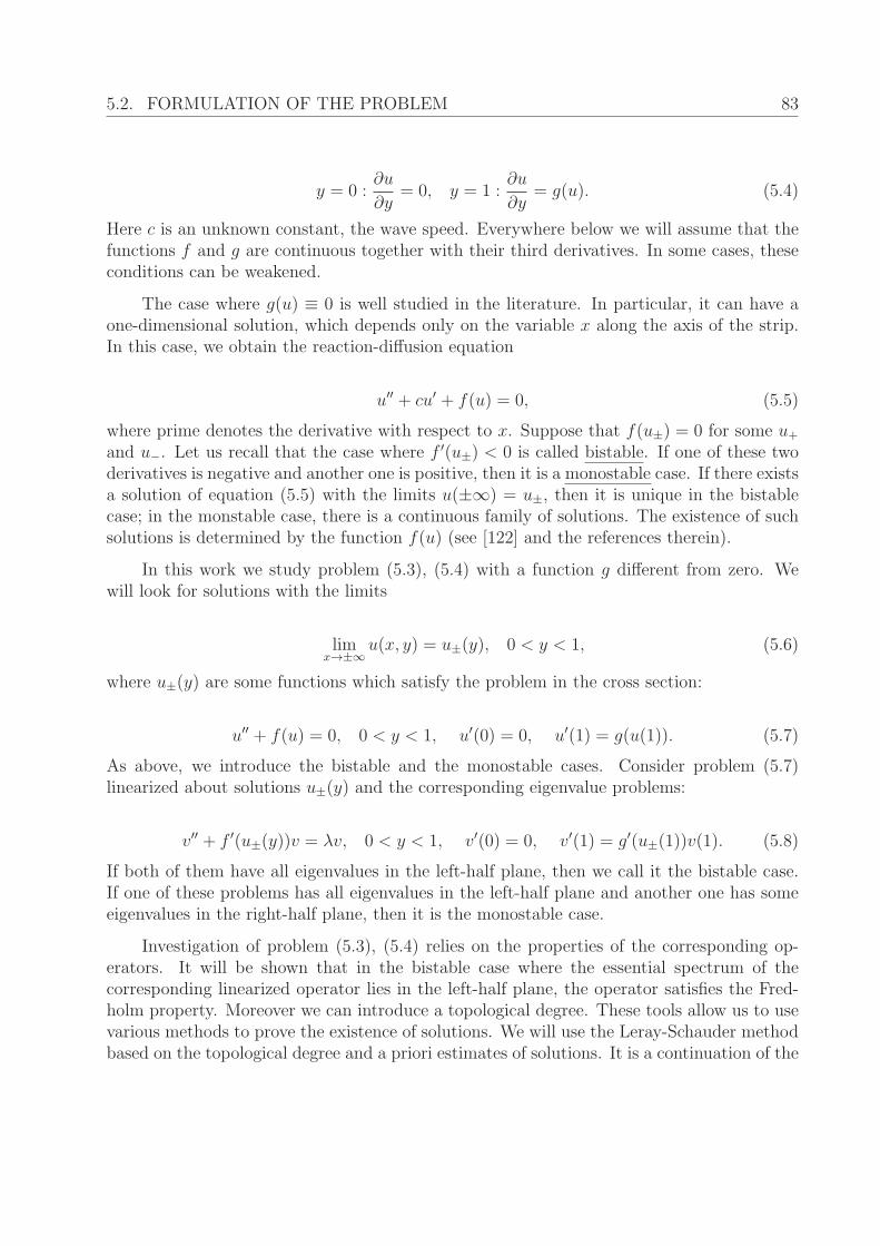
5.2. FORMULATION OF THE PROBLEM 83
y = 0 :∂u
∂y= 0, y = 1 :
∂u
∂y= g(u). (5.4)
Here c is an unknown constant, the wave speed. Everywhere below we will assume that thefunctions f and g are continuous together with their third derivatives. In some cases, theseconditions can be weakened.
The case where g(u) ≡ 0 is well studied in the literature. In particular, it can have aone-dimensional solution, which depends only on the variable x along the axis of the strip.In this case, we obtain the reaction-diffusion equation
u′′ + cu′ + f(u) = 0, (5.5)
where prime denotes the derivative with respect to x. Suppose that f(u±) = 0 for some u+
and u−. Let us recall that the case where f ′(u±) < 0 is called bistable. If one of these twoderivatives is negative and another one is positive, then it is a monostable case. If there existsa solution of equation (5.5) with the limits u(±∞) = u±, then it is unique in the bistablecase; in the monstable case, there is a continuous family of solutions. The existence of suchsolutions is determined by the function f(u) (see [122] and the references therein).
In this work we study problem (5.3), (5.4) with a function g different from zero. Wewill look for solutions with the limits
limx→±∞
u(x, y) = u±(y), 0 < y < 1, (5.6)
where u±(y) are some functions which satisfy the problem in the cross section:
u′′ + f(u) = 0, 0 < y < 1, u′(0) = 0, u′(1) = g(u(1)). (5.7)
As above, we introduce the bistable and the monostable cases. Consider problem (5.7)linearized about solutions u±(y) and the corresponding eigenvalue problems:
v′′ + f ′(u±(y))v = λv, 0 < y < 1, v′(0) = 0, v′(1) = g′(u±(1))v(1). (5.8)
If both of them have all eigenvalues in the left-half plane, then we call it the bistable case.If one of these problems has all eigenvalues in the left-half plane and another one has someeigenvalues in the right-half plane, then it is the monostable case.
Investigation of problem (5.3), (5.4) relies on the properties of the corresponding op-erators. It will be shown that in the bistable case where the essential spectrum of thecorresponding linearized operator lies in the left-half plane, the operator satisfies the Fred-holm property. Moreover we can introduce a topological degree. These tools allow us to usevarious methods to prove the existence of solutions. We will use the Leray-Schauder methodbased on the topological degree and a priori estimates of solutions. It is a continuation of the
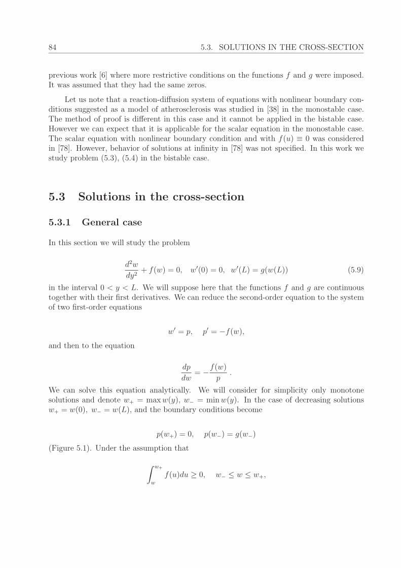
84 5.3. SOLUTIONS IN THE CROSS-SECTION
previous work [6] where more restrictive conditions on the functions f and g were imposed.It was assumed that they had the same zeros.
Let us note that a reaction-diffusion system of equations with nonlinear boundary con-ditions suggested as a model of atherosclerosis was studied in [38] in the monostable case.The method of proof is different in this case and it cannot be applied in the bistable case.However we can expect that it is applicable for the scalar equation in the monostable case.The scalar equation with nonlinear boundary condition and with f(u) ≡ 0 was consideredin [78]. However, behavior of solutions at infinity in [78] was not specified. In this work westudy problem (5.3), (5.4) in the bistable case.
5.3 Solutions in the cross-section
5.3.1 General case
In this section we will study the problem
d2w
dy2+ f(w) = 0, w′(0) = 0, w′(L) = g(w(L)) (5.9)
in the interval 0 < y < L. We will suppose here that the functions f and g are continuoustogether with their first derivatives. We can reduce the second-order equation to the systemof two first-order equations
w′ = p, p′ = −f(w),
and then to the equation
dp
dw= −f(w)
p.
We can solve this equation analytically. We will consider for simplicity only monotonesolutions and denote w+ = maxw(y), w− = minw(y). In the case of decreasing solutionsw+ = w(0), w− = w(L), and the boundary conditions become
p(w+) = 0, p(w−) = g(w−)
(Figure 5.1). Under the assumption that
∫ w+
w
f(u)du ≥ 0, w− ≤ w ≤ w+,
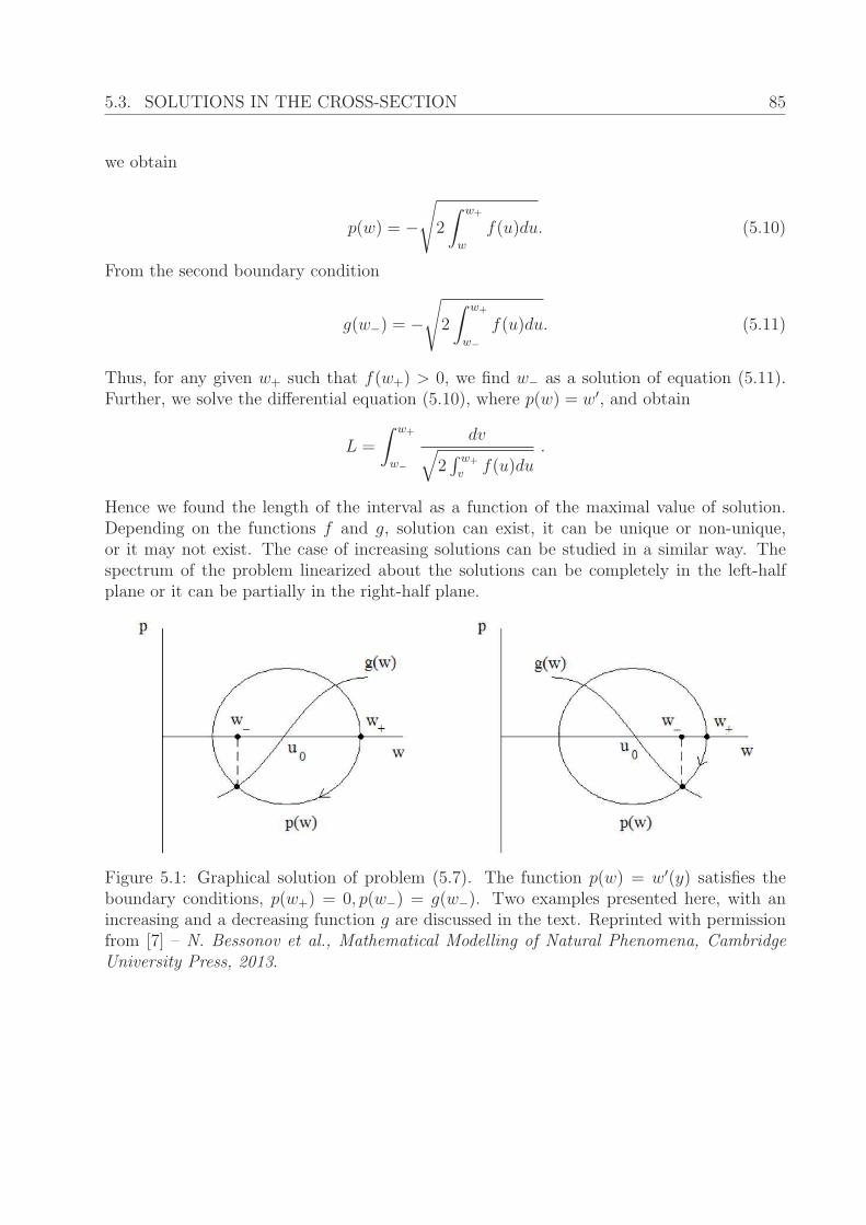
5.3. SOLUTIONS IN THE CROSS-SECTION 85
we obtain
p(w) = −√
2
∫ w+
w
f(u)du. (5.10)
From the second boundary condition
g(w−) = −√
2
∫ w+
w−f(u)du. (5.11)
Thus, for any given w+ such that f(w+) > 0, we find w− as a solution of equation (5.11).Further, we solve the differential equation (5.10), where p(w) = w′, and obtain
L =
∫ w+
w−
dv√2∫ w+
vf(u)du
.
Hence we found the length of the interval as a function of the maximal value of solution.Depending on the functions f and g, solution can exist, it can be unique or non-unique,or it may not exist. The case of increasing solutions can be studied in a similar way. Thespectrum of the problem linearized about the solutions can be completely in the left-halfplane or it can be partially in the right-half plane.
Figure 5.1: Graphical solution of problem (5.7). The function p(w) = w′(y) satisfies theboundary conditions, p(w+) = 0, p(w−) = g(w−). Two examples presented here, with anincreasing and a decreasing function g are discussed in the text. Reprinted with permissionfrom [7] – N. Bessonov et al., Mathematical Modelling of Natural Phenomena, CambridgeUniversity Press, 2013.
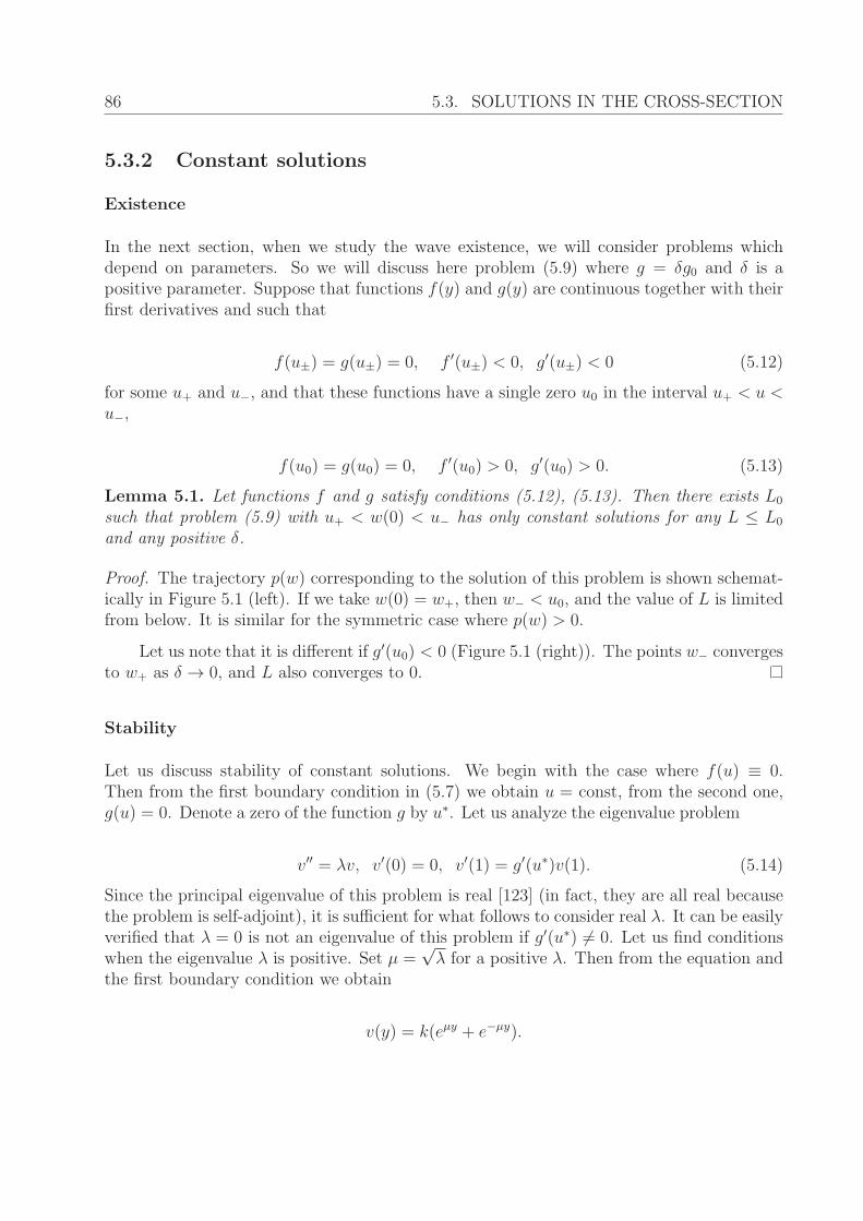
86 5.3. SOLUTIONS IN THE CROSS-SECTION
5.3.2 Constant solutions
Existence
In the next section, when we study the wave existence, we will consider problems whichdepend on parameters. So we will discuss here problem (5.9) where g = δg0 and δ is apositive parameter. Suppose that functions f(y) and g(y) are continuous together with theirfirst derivatives and such that
f(u±) = g(u±) = 0, f ′(u±) < 0, g′(u±) < 0 (5.12)
for some u+ and u−, and that these functions have a single zero u0 in the interval u+ < u <u−,
f(u0) = g(u0) = 0, f ′(u0) > 0, g′(u0) > 0. (5.13)
Lemma 5.1. Let functions f and g satisfy conditions (5.12), (5.13). Then there exists L0
such that problem (5.9) with u+ < w(0) < u− has only constant solutions for any L ≤ L0
and any positive δ.
Proof. The trajectory p(w) corresponding to the solution of this problem is shown schemat-ically in Figure 5.1 (left). If we take w(0) = w+, then w− < u0, and the value of L is limitedfrom below. It is similar for the symmetric case where p(w) > 0.
Let us note that it is different if g′(u0) < 0 (Figure 5.1 (right)). The points w− convergesto w+ as δ → 0, and L also converges to 0.
Stability
Let us discuss stability of constant solutions. We begin with the case where f(u) ≡ 0.Then from the first boundary condition in (5.7) we obtain u = const, from the second one,g(u) = 0. Denote a zero of the function g by u∗. Let us analyze the eigenvalue problem
v′′ = λv, v′(0) = 0, v′(1) = g′(u∗)v(1). (5.14)
Since the principal eigenvalue of this problem is real [123] (in fact, they are all real becausethe problem is self-adjoint), it is sufficient for what follows to consider real λ. It can be easilyverified that λ = 0 is not an eigenvalue of this problem if g′(u∗) = 0. Let us find conditionswhen the eigenvalue λ is positive. Set μ =
√λ for a positive λ. Then from the equation and
the first boundary condition we obtain
v(y) = k(eμy + e−μy).
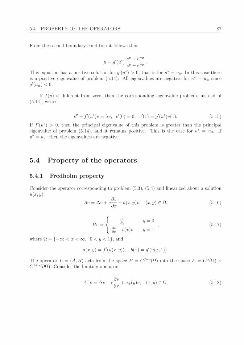
5.4. PROPERTY OF THE OPERATORS 87
From the second boundary condition it follows that
μ = g′(u∗)eμ + e−μ
eμ − e−μ.
This equation has a positive solution for g′(u∗) > 0, that is for u∗ = u0. In this case thereis a positive eigenvalue of problem (5.14). All eigenvalues are negative for u∗ = u± sinceg′(u±) < 0.
If f(u) is different from zero, then the corresponding eigenvalue problem, instead of(5.14), writes
v′′ + f ′(u∗)v = λv, v′(0) = 0, v′(1) = g′(u∗)v(1). (5.15)
If f ′(u∗) > 0, then the principal eigenvalue of this problem is greater than the principaleigenvalue of problem (5.14), and it remains positive. This is the case for u∗ = u0. Ifu∗ = u±, then the eigenvalues are negative.
5.4 Property of the operators
5.4.1 Fredholm property
Consider the operator corresponding to problem (5.3), (5.4) and linearized about a solutionu(x, y):
Av = Δv + c∂v
∂x+ a(x, y)v, (x, y) ∈ Ω, (5.16)
Bv =
⎧⎨⎩ ∂v∂y
, y = 0
∂v∂y
− b(x)v , y = 1, (5.17)
where Ω = {−∞ < x < ∞, 0 < y < 1}, and
a(x, y) = f ′(u(x, y)), b(x) = g′(u(x, 1)).
The operator L = (A,B) acts from the space E = C2+α(Ω) into the space F = Cα(Ω) ×C1+α(∂Ω). Consider the limiting operators
A±v = Δv + c∂v
∂x+ a±(y)v, (x, y) ∈ Ω, (5.18)
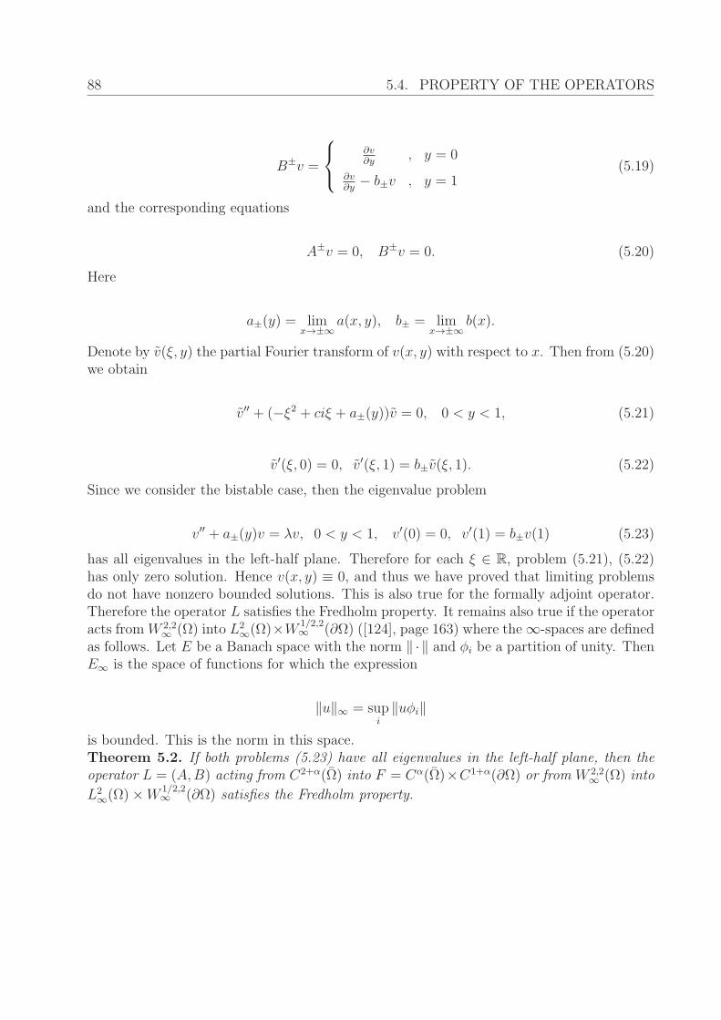
88 5.4. PROPERTY OF THE OPERATORS
B±v =
⎧⎨⎩ ∂v∂y
, y = 0
∂v∂y
− b±v , y = 1(5.19)
and the corresponding equations
A±v = 0, B±v = 0. (5.20)
Here
a±(y) = limx→±∞
a(x, y), b± = limx→±∞
b(x).
Denote by v(ξ, y) the partial Fourier transform of v(x, y) with respect to x. Then from (5.20)we obtain
v′′ + (−ξ2 + ciξ + a±(y))v = 0, 0 < y < 1, (5.21)
v′(ξ, 0) = 0, v′(ξ, 1) = b±v(ξ, 1). (5.22)
Since we consider the bistable case, then the eigenvalue problem
v′′ + a±(y)v = λv, 0 < y < 1, v′(0) = 0, v′(1) = b±v(1) (5.23)
has all eigenvalues in the left-half plane. Therefore for each ξ ∈ R, problem (5.21), (5.22)has only zero solution. Hence v(x, y) ≡ 0, and thus we have proved that limiting problemsdo not have nonzero bounded solutions. This is also true for the formally adjoint operator.Therefore the operator L satisfies the Fredholm property. It remains also true if the operatoracts from W 2,2
∞ (Ω) into L2∞(Ω)×W
1/2,2∞ (∂Ω) ([124], page 163) where the ∞-spaces are defined
as follows. Let E be a Banach space with the norm ‖ · ‖ and φi be a partition of unity. ThenE∞ is the space of functions for which the expression
‖u‖∞ = supi
‖uφi‖
is bounded. This is the norm in this space.Theorem 5.2. If both problems (5.23) have all eigenvalues in the left-half plane, then theoperator L = (A,B) acting from C2+α(Ω) into F = Cα(Ω)×C1+α(∂Ω) or from W 2,2
∞ (Ω) into
L2∞(Ω)×W
1/2,2∞ (∂Ω) satisfies the Fredholm property.
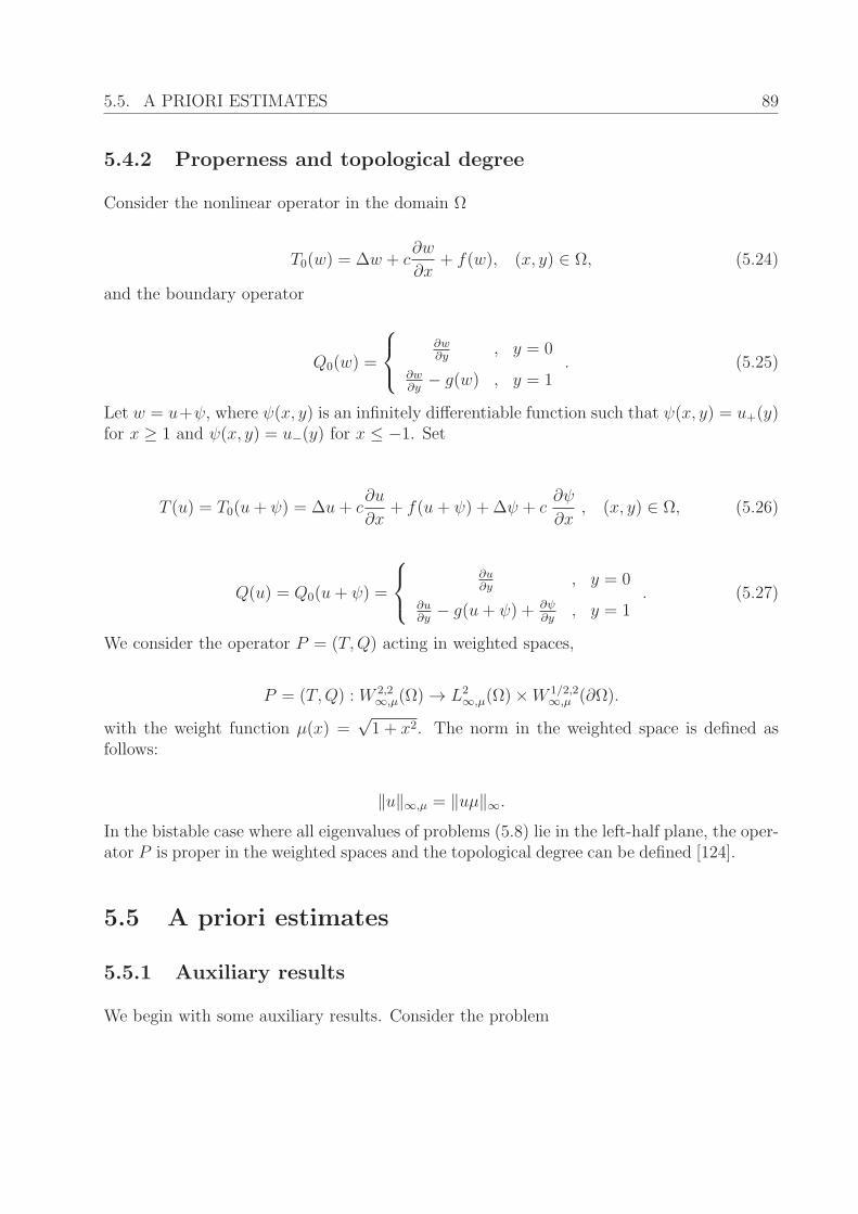
5.5. A PRIORI ESTIMATES 89
5.4.2 Properness and topological degree
Consider the nonlinear operator in the domain Ω
T0(w) = Δw + c∂w
∂x+ f(w), (x, y) ∈ Ω, (5.24)
and the boundary operator
Q0(w) =
⎧⎨⎩ ∂w∂y
, y = 0
∂w∂y
− g(w) , y = 1. (5.25)
Let w = u+ψ, where ψ(x, y) is an infinitely differentiable function such that ψ(x, y) = u+(y)for x ≥ 1 and ψ(x, y) = u−(y) for x ≤ −1. Set
T (u) = T0(u+ ψ) = Δu+ c∂u
∂x+ f(u+ ψ) + Δψ + c
∂ψ
∂x, (x, y) ∈ Ω, (5.26)
Q(u) = Q0(u+ ψ) =
⎧⎨⎩ ∂u∂y
, y = 0
∂u∂y
− g(u+ ψ) + ∂ψ∂y
, y = 1. (5.27)
We consider the operator P = (T,Q) acting in weighted spaces,
P = (T,Q) : W 2,2∞,μ(Ω) → L2
∞,μ(Ω)×W 1/2,2∞,μ (∂Ω).
with the weight function μ(x) =√1 + x2. The norm in the weighted space is defined as
follows:
‖u‖∞,μ = ‖uμ‖∞.
In the bistable case where all eigenvalues of problems (5.8) lie in the left-half plane, the oper-ator P is proper in the weighted spaces and the topological degree can be defined [124].
5.5 A priori estimates
5.5.1 Auxiliary results
We begin with some auxiliary results. Consider the problem
90 5.5. A PRIORI ESTIMATES
Δu+ c∂u
∂x+ f(u) = 0, (5.28)
y = 0 :∂u
∂y= 0, y = 1 :
∂u
∂y= g(u). (5.29)
We look for the solutions with the limits
limx→±∞
u(x, y) = u±(y), 0 < y < 1 (5.30)
at infinity, u−(y) > u+(y). The proofs of the following lemmas are similar to those in [6].
Lemma 5.3. Let U0(x, y) be a solution of problem (5.28), (5.29) such that ∂U0
∂x≤ 0 for all
(x, y) ∈ Ω. Then the last inequality is strict.
Lemma 5.4. Let un(x, y) be a sequence of solutions of problem (5.28), (5.29) such thatun → U0 in C1(Ω), where U0(x, y) is a solution monotonically decreasing with respect to x.Then for all n sufficiently large ∂un
∂x< 0, (x, y) ∈ Ω.
We will now determine the sign of the speed of the wave connecting a stable and anunstable solutions. This result will be used below for estimates of solutions.
Lemma 5.5. Suppose u0(y) is a solution of problem (5.7) in the cross section of the domain,and u+(y) < u0(y) < u−(y). Assume, next, that the corresponding eigenvalue problem
v′′ + f ′(u0)v = λv, v′(0) = 0, v′(1) = g′(u0(1))v(1) (5.31)
has some eigenvalues in the right-half plane. If a monotone with respect to x function w(x, y)satisfies the problem
Δw + c∂w
∂x+ f(w) = 0, (5.32)
y = 0 :∂w
∂y= 0, y = 1 :
∂w
∂y= g(w), (5.33)
limx→−∞
w(x, y) = u−(y), limx→∞
w(x, y) = u0(y), (5.34)
then c > 0. If
limx→−∞
w(x, y) = u0(y), limx→∞
w(x, y) = u+(y),
5.5. A PRIORI ESTIMATES 91
instead of (5.34), then c < 0.
Lemma 5.6. If problem (5.28)-(5.30) has a solution w, then the value of the speed admitsthe estimate |c| ≤ M , where the constant M depends only on maxu∈[u+,u−] |f ′(u)|, |g′(u)|.
5.5.2 Functionalization of the parameter
Let w0(x, y) be a solution of problem (5.28)-(5.30). Then the functions
wh(x, y) = w0(x+ h, y), h ∈ R
are also solutions of this problem. The existence of the family of solutions does not allowone to use directly the topological degree because there is a zero eigenvalue of the linearizedproblem and a uniform a priori estimate of solutions in the weighted spaces does not oc-cur.
In order to overcome this difficulty, we replace the unknown parameter c, the wavespeed, by a functional c(wh). This approach was suggested in [76] for periodic solutions ofordinary differential systems of equations, and then used for travelling waves in [122]. Thisfunctional determines a function of h, s(h) = c(wh). We will construct this functional insuch a way that s′(h) < 0 and s(h) → ±∞ as h → ∓∞. Then instead of the family ofsolutions we obtain a single solution for the value of h for which c = s(h).
Let
ρ(wh) =
∫Ω
(w0(x+ h, y)− u+(y))r(x)dxdy,
where r(x) is an increasing function satisfying the conditions:
r(−∞) = 0, r(+∞) = 1,
∫ 0
−∞r(x)dx < ∞.
Since w0(x, y) is a decreasing function of x, then ρ(wh) is a decreasing function of h, and
ρ(wh) →⎧⎨⎩ 0 , h → +∞
+∞ , h → −∞.
Hence the function s(h) = c(wh) = ln ρ(wh) possesses the required properties.
92 5.5. A PRIORI ESTIMATES
5.5.3 Estimates of solutions
We consider next the problem
Δw + c∂w
∂x+ fτ (w) = 0, (5.35)
y = 0 :∂w
∂y= 0, y = 1 :
∂w
∂y= gτ (w), (5.36)
w(±∞, y) = u±(y), (5.37)
where the functions f and g depend on the parameter τ ∈ [0, 1]. Everywhere below wewill assume that the functions fτ (w), gτ (w) are bounded and continuous together with theirderivatives of the third order with respect to w and of the second order with respect to τ .These conditions allow the construction of the topological degree [124].
The proof of the following lemma is given in the appendix.
Lemma 5.7. Suppose that solution w(x, y) of problem (5.35)-(5.37) satisfies the estimate|w| ≤ M with some positive constant M , and
|f (i)τ (w)|, |g(i)τ (w)| ≤ K for |w| ≤ M, i = 0, 1, 2, 3,
where K is a positive constant. Then the Holder norm C2+α(Ω), 0 < α < 1 of the solutionis bounded by a constant which depends only on K, M and c.
Denote by wτ a solution of problem (5.35)-(5.37). We need to obtain a uniform estimateof the solution uτ = wτ − ψ in the norm of the space W 2,2
∞,μ(Ω). Here ψ(x, y) is an infinitelydifferentiable function such that ψ(x, y) = u+(y) for x ≥ 1 and ψ(x, y) = u−(y) for x ≤ −1.Since u ∈ C2+α(Ω), then the norm W 2,2
∞ (Ω) of the solution is also uniformly bounded.However, the boundedness of the norm in the weighted space does not follow from this andshould be proved. In order to obtain the estimate, it is sufficient to prove that the solutionis bounded in the weighted space, that is
sup(x,y)∈Ω
|(wτ (x, y)− ψ(x, y))μ(x)| ≤ M (5.38)
with some constant M independent of τ . If this estimate is satisfied, then the derivatives ofthe solution up to the order two are also bounded. Indeed, the function uτ = wτ −ψ satisfiesthe problem
Δu+ c∂u
∂x+ f(u+ ψ) + γ(x, y) = 0,
5.5. A PRIORI ESTIMATES 93
y = 0 :∂u
∂y= 0, y = 1 :
∂u
∂y= g(u+ ψ),
where γ(x, y) = Δψ + c∂ψ∂x. Then the function vτ = uτμ satisfies the problem
Δv + (c− 2μ1)∂v
∂x+ (−cμ1 + 2μ2
1 − μ2)v + (f(u+ ψ)− f(ψ))μ+ (γ + f(ψ))μ = 0, (5.39)
y = 0 :∂v
∂y= 0, y = 1 :
∂v
∂y= (g(u+ ψ)− g(ψ))μ+ g(ψ)μ, (5.40)
where
μ1 =μ′
μ, μ2 =
μ′′
μ
are bounded infinitely differentiable functions converging to zero at infinity. Since
|(f(u+ ψ)− f(ψ))μ| ≤ sups
|f ′(s)||uμ|, |(g(u+ ψ)− g(ψ))μ| ≤ sups
|g′(s)||uμ|,
then, by virtue of (5.38), the functions
Φ(u, x) = (f(u+ ψ)− f(ψ))μ+ (γ + f(ψ))μ, Ψ(u, x) = (g(u+ ψ)− g(ψ))μ+ g(ψ)μ
are bounded together with their second derivatives. Therefore solutions of problem (5.39),(5.40) are uniformly bounded in the space C2+α(Ω). Then the normW 2,2
∞ (Ω) is also bounded.
It remains to prove estimate (5.38). Consider first of all the behavior of solutions at thevicinity of infinity. By virtue of the Fredholm property, |wτ (x, y)−u±(y)| decay exponentiallyas x → ±∞. The decay rate is determined by the principal eigenvalue of the correspondingoperators in the cross-section of the cylinder. They can be estimated independently ofτ .
Let ε > 0 be small enough, N−(τ) and N+(τ) be such that |wτ (x, y) − u+(y)| ≤ ε forx ≥ N+(τ) and |wτ (x, y)−u−(y)| ≤ ε for x ≤ N−(τ). For a polynomial weight function μ(x)there exists a constant K independent of τ ∈ [0, 1] such that
|wτ (x, y)− u±(y)|μ(x) ≤ K, x ≷ N±(τ), τ ∈ [0, 1].
Since the functions wτ (x, y) are uniformly bounded, then (5.38) will follow from the uniformboundedness of the values N±(τ).
94 5.6. LERAY-SCHAUDER METHOD
First, let us note that the difference between them is uniformly bounded. Indeed, if thisis not the case and N+(τ)−N−(τ) → ∞ as τ → τ0 for some τ0, then there are two solutionsof problem (5.35), (5.36) for τ = τ0, w1 and w2 with the limits
w1(x, y) →⎧⎨⎩ u−(y) , x → −∞
u0(y) , x → +∞, w2(x, y) →
⎧⎨⎩ u0(y) , x → −∞u+(y) , x → +∞
.
These solutions are obtained as limits of the solution wτ as τ → τ0. In order to obtain them,consider a sequence of functions wτk(x, y), τk → τ0 and two sequences of shifted functions:wτk(x + N−(τk), y) and wτk(x + N+(τk), y). The first sequence gives in the limit the firstsolution, the second limit gives the second solution.
The existence of such solutions contradicts Lemma 5.5 since the first one affirms thatthe speed is positive while the second one that it is negative.
Next, if one of the values |N±(τ)| tends to infinity as τ → τ0, then the modulus |c(wh)|of the functional introduced in Section 4.1 also tends to infinity as τ → τ0. This contradictsa priori estimates of the wave speed. Thus, we have proved the following theorem.
Theorem 5.8. Let the functions fτ (w), gτ (w) be bounded and continuous together with theirderivatives of the third order with respect to w and of the second order with respect to τ . Ifthere exists a solution wτ of problem (5.35)-(5.37) such that uτ = wτ − ψ ∈ W 2,2
∞,μ(Ω), thenthe norm ‖uτ‖W 2,2∞,μ(Ω) is bounded independently of τ and of the solution wτ .
5.6 Leray-Schauder method
5.6.1 Model problem
Consider the problem
Δw + c∂w
∂x+ f(w) = 0, (5.1)
y = 0 :∂w
∂y= 0, y = 1 :
∂w
∂y= 0, (5.2)
w(±∞, y) = u±, (5.3)
where we put 0 instead of g(w) in the boundary condition, u+ and u− are some numberssuch that f(u±) = 0, f ′(u±) < 0. Suppose that there exists a single zero u0 of the function

5.6. LERAY-SCHAUDER METHOD 95
f in the interval (u+, u−), f ′(u0) > 0. Less restrictive conditions on the function f can alsobe considered. In this case the problem
w′′ + cw′ + f(w) = 0, w(±∞) = u±
has a solution w0(x) for a unique value of c (see, e.g., [122]). This function is also a solutionof problem (5.1)-(5.3). The uniqueness of this solution as a solution of the two-dimensionalproblem is proved in the following lemma.
Lemma 5.9. There exists a unique monotone in x solution of problem (5.1)-(5.3) up totranslation in space.
Proof. Suppose that there exist two different monotone solutions of problem (5.1)-(5.3),(w1, c1) and (w2, c2). We recall that the corresponding values of the speed c can be different.Consider the equation
∂v
∂t= Δv + c1
∂v
∂x+ f(v) (5.4)
with the boundary condition (5.2). The function w1(x, y) is a stationary solution of thisproblem. It is proved in [123] that it is globally stable with respect to all initial condi-tions v(x, y, 0), which are monotone with respect to x and such that the norm ‖v(x, y, 0)−w1(x, y)‖L2(Ω) is bounded.
Consider the initial condition v(x, y, 0) = w2(x, y). It is monotone and the L2 norm ofthe difference w2 − w1 is bounded since these functions approach exponentially their limitsat infinity. According to the stability result, the solution converges to w1(x+h, y) with someh. On the other hand, the solution writes u(x, y, t) = w2(x − (c2 − c1)t, y), and it cannotconverge to w1. This contradiction proves the lemma.
We consider next the problem (5.35)-(5.37) and the corresponding operators
Tτ (u) = Δ(u+ ψ) + c(u+ ψ)∂(u+ ψ)
∂x+ fτ (u+ ψ), (x, y) ∈ Ω, (5.5)
Qτ (u) =
⎧⎨⎩ ∂u∂y
, y = 0
∂u∂y
− gτ (u+ ψ) , y = 1, (5.6)
Pτ = (Tτ , Qτ ) : W2,2∞,μ(Ω) → L2
∞,μ(Ω)×W 1/2,2∞,μ (∂Ω).
Suppose that gτ (u) ≡ 0 for τ = 0. Then the equation
96 5.6. LERAY-SCHAUDER METHOD
Pτ (u) = 0 (5.7)
has a unique solution u0 = w0 − ψ for τ = 0. The index of this solution, that is thetopological degree of this operator with respect to a small neighborhood of the solution,equal 1. Indeed, the index equals (−1)ν , where the ν is the number of positive eigenvalues ofthe linearized operator [122], [124]. In the case under consideration, the linearized operatorhas all eigenvalues in the left-half plane [123].
5.6.2 Wave existence
As above, we assume that the functions fτ (w), gτ (w) are bounded and continuous togetherwith their derivatives of the third order with respect to w and of the second order withrespect to τ . We begin with a general result on wave existence.
Theorem 5.10. Let the problem
d2w
dy2+ fτ (w) = 0, w′(0) = 0, w′(L) = gτ (w(L)) (5.8)
have solutions uτ±(y) such that
uτ+(y) < uτ−(y), 0 ≤ y ≤ L
and the eigenvalue problems
d2v
dy2+ f ′
τ (uτ±)v = λv, v′(0) = 0, v′(L) = g′τ (u
τ±)v(L) (5.9)
have all eigenvalues in the left-half plane for any τ ∈ [0, 1]. Suppose that for any othersolution uτ0(y) of problem (5.8), the eigenvalue problem
d2v
dy2+ f ′
τ (uτ0)v = λv, v′(0) = 0, v′(L) = g′τ (u
τ0)v(L) (5.10)
has some eigenvalues in the right-half plane. If the problem
Δw + c∂w
∂x+ fτ (w) = 0, (5.11)
y = 0 :∂w
∂y= 0, y = L :
∂w
∂y= gτ (w), (5.12)
5.6. LERAY-SCHAUDER METHOD 97
limx→±∞
w(x, y) = uτ±(y), 0 < y < L, (5.13)
considered in the domain Ω = {−∞ < x < ∞, 0 < y < L}, has a unique solution monotonewith respect to x for τ = 0, then it also has a unique monotone solution for any τ ∈ [0, 1].
Proof. The proof of the theorem is based on the Leray-Schauder method. We considerequation (5.7). The topological degree for the operator Pτ (u) is defined (Section 3).
Denote by Γm the ensemble of solutions of equation (5.7) for all τ ∈ [0, 1] such thatfor any u ∈ Γm the function w = u + ψ is monotone with respect to x. Let Γn be theset of all solutions for which the function w = u + ψ is not monotone with respect to x.Then the distance d between these two sets in the space E = W 2,2
∞,μ(Ω) is positive. Indeed,suppose that this is not true. Then there exist two sequences uk ∈ Γm and vk ∈ Γn suchthat ‖uk − vk‖E → 0 as k → ∞. From Lemma 5.4 it follows that the functions wk = vk + ψare monotone with respect to x for k sufficiently large. This contradiction shows that theconvergence cannot occur.
From Theorem 5.8, applicable for solutions from Γm, it follows that the set Γm isbounded in E. Moreover, by virtue of properness of the operator Pτ it is compact. Hencethere exists a bounded domain G ⊂ E such that Γm ⊂ G and Γn ∩ G = �.
Consider the topological degree γ(Pτ , G). Since
Pτ (u) = 0, u ∈ ∂G,
then it is well defined. Since γ(P0, G) = 1 (Section 6.1), then γ(Pτ , G) = 1 for any τ ∈ [0, 1].Hence problem (5.11)-(5.13) has a monotone solution for any τ ∈ [0, 1].
It remains to verify its uniqueness. We recall that
γ(Pτ , G) =∑i
ind ui,
where ind ui is the index of a solution ui and the sum is taken with respect to all solutionsui ∈ G. Since γ(Pτ , G) = 1 and ind ui = 1 (cf. Section 5.1), then the solution is necessarilyunique.
The previous theorem uses some assumptions about the solutions uτ± and uτ0 of problem(5.8) in the cross-section. We will now consider some particular cases where these conditionscan be verified.
Theorem 5.11. Let u+ and u− be some constants and the following conditions be satisfied:
1. f(u±) = 0, f ′(u±) < 0 , g(u±) = 0, g′(u±) < 0 ,
98 5.6. LERAY-SCHAUDER METHOD
2. f(u0) = 0, f ′(u0) > 0 , g(u0) = 0, g′(u0) > 0 for some u0 ∈ (u+, u−), and there are noother zeros of these functions in this interval.
Then for all positive L sufficiently small, the problem
Δw + c∂w
∂x+ f(w) = 0, (5.14)
y = 0 :∂w
∂y= 0, y = L :
∂w
∂y= g(w), (5.15)
limx→±∞
w(x, y) = u± (5.16)
considered in the domain Ω = {−∞ < x < ∞, 0 < y < L} has a unique solution monotonewith respect to x.
This theorem follows from the previous one, where we set gτ = τg, and from Lemmas5.4 and 5.9
Theorem 5.12. Let the function g(w) satisfy conditions of the previous theorem. Then forall positive L, the problem
Δw + c∂w
∂x= 0, (5.17)
y = 0 :∂w
∂y= 0, y = L :
∂w
∂y= g(w), (5.18)
limx→±∞
w(x, y) = u± (5.19)
considered in the domain Ω = {−∞ < x < ∞, 0 < y < L} has a unique solution monotonewith respect to x.
Proof. The proof consists of two steps. First, we consider sufficiently small L and use theresult of the previous theorem as a starting point for the deformation fτ = (1 − τ)f . Forτ = 1 we obtain fτ (w) ≡ 0. At the next step, we increase the width L of the domain. It isequivalent to the change of variables y = ση in the equation and in the boundary condition.The problem in the cross-section has only constant solutions. We can use the results ofSection 2.2 about their stability and Theorem 5.10.
In the last theorem we consider the case of small boundary conditions where the solutionis close to a one-dimensional solution.
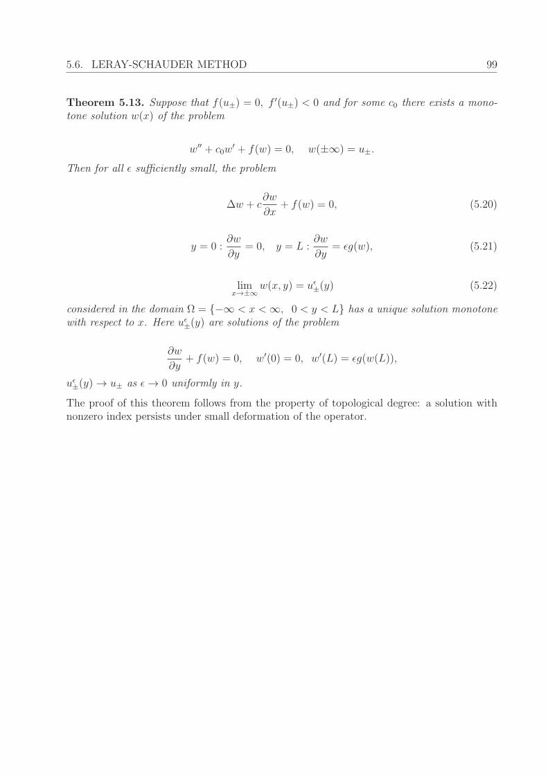
5.6. LERAY-SCHAUDER METHOD 99
Theorem 5.13. Suppose that f(u±) = 0, f ′(u±) < 0 and for some c0 there exists a mono-tone solution w(x) of the problem
w′′ + c0w′ + f(w) = 0, w(±∞) = u±.
Then for all ε sufficiently small, the problem
Δw + c∂w
∂x+ f(w) = 0, (5.20)
y = 0 :∂w
∂y= 0, y = L :
∂w
∂y= εg(w), (5.21)
limx→±∞
w(x, y) = uε±(y) (5.22)
considered in the domain Ω = {−∞ < x < ∞, 0 < y < L} has a unique solution monotonewith respect to x. Here uε±(y) are solutions of the problem
∂w
∂y+ f(w) = 0, w′(0) = 0, w′(L) = εg(w(L)),
uε±(y) → u± as ε → 0 uniformly in y.
The proof of this theorem follows from the property of topological degree: a solution withnonzero index persists under small deformation of the operator.

101
Conclusion and Perspectives
Conclusions. This thesis is devoted to discrete and continuous modelling of blood flowsand related phenomena such as blood coagulation and atherosclerosis. The main results ofthe dissertation are as follows:
1. Modelling of blood flow with a discrete particle method was carried out. Blood plasmaflow was modelled by Dissipative Particle Dynamics (DPD) in 2D. Various implemen-tations of blood flow model and boundary conditions in DPD were introduced andinvestigated in order to obtain a correct description of the fluid flow appropriate forthe investigation of blood coagulation. A complex combination of simulation domainpartition and boundary conditions was developed that is suitable for modelling of bloodcoagulation. Furthermore, a model of the erythrocyte membrane suitable for use inthe DPD method was proposed and investigated.
2. A discrete model of platelet aggregation in flow was proposed. The DPD method wasused to model blood plasma flow and platelets suspended in it. Platelet clot growthin flow was studied, depending on inter-platelet adhesion forces. Finally, a possiblemechanism of platelet clot growth arrest in flow was suggested.
3. Two hybrid models of platelet and fibrin clot were proposed and investigated. Theycombine discrete (DPD) and continuous (PDE) methods, describing platelets sus-pended in plasma and concentrations of blood factors in flow respectfully. The firsthybrid model was used to study the interaction between a platelet clot and a fibrinconcentration in flow. The second hybrid model introduced a more realistic sub-modelof coagulation pathways, accounting for its main characteristics. The model was usedto study the interaction of platelet and fibrin clot, showing a possible mechanism bywhich the platelet clot stops growing and limits the further growth of the fibrin net.Furthermore, the influence of the flow speed on the clot formation was investigated inthe scope of this model.
4. A mathematical analysis of a model of chronic inflammation related to atherosclerosiswas carried out. A problem describing the propagation of a reaction-diffusion wave inthe 2D case with nonlinear boundary conditions was studied. The existence of waves inthe bistable case was proven using the Leray-Schauder method and a priori estimatesof solutions.
102
5. Numerical implementations of the discrete and hybrid models describing blood flow andblood coagulation were done in the framework of this thesis. Due to the significantcomputational cost of such models, different optimisation techniques were used. Thenumerical code was parallelized on both Central Processing Unit (CPU) and GraphicalProcessing Unit (GPU), and the performances were compared.
Perspectives. The models developed in the thesis concern blood flows and cell interactionswith the focus on blood coagulation. They offer many possibilities for future research anddevelopment:
– Studies of the properties of blood cells and their interactions in flow, such as the bloodcell distribution in flow [15, 16].
– Further advances in the modelling of blood coagulation with a more complete modelsuitable for medical applications:
- modelling of blood coagulation in 3D and quantitative comparison with experi-mental results,
- investigation of the influence of erythrocyte distribution on clot growth in flow,
- introduction of a more complete model of blood coagulation pathways and aconsequent study of the sensitivity of the model and its impact on clot formationin flow,
- modelling of the initiation of the coagulation process in flow, as an important firststep in the blood coagulation process,
- modelling of primary fibrinolysis, the process of blood clot decomposition in nor-mal conditions, and secondary fibrinolysis due to a medical disorder, medicaltreatment, or other cause,
- modelling of pathological clot growth related to many diseases and disorders, suchas atherosclerosis or arthritis.
- investigation of pulsatile flow influence on clot growth in flow.
– Modelling of atherosclerosis and atherosclerotic plaque development by the same ap-proach (DPD-PDE hybrid method).
We intend to study these questions in the future works.
103
Publications
The results of the thesis are presented in the following publications:
1. A. Tosenberger, F. Ataullakhanov, N. Bessonov, M. Panteleev, A. Tokarev, V. Volpert,Modelling of clot growth in flow with a DPD-PDE method, Journal of TheoreticalBiology 337, (2013), pp. 30-41.
2. V. Volpert, N. Bessonov, N. Eymard, A. Tosenberger, Modele multi-echelle de la dy-namique cellulaire, Le vivant discret et continu, Editions Materiologiques (Ed.), (2013),ISBN : 978-2-919694-23-5.
3. N. Bessonov, E. Babushkina, S.F. Golovashchenko, A. Tosenberger, F. Ataullakhanov,M. Panteleev, A. Tokarev, V. Volpert, Numerical Modelling of Cell Distribution inBlood Flow, Math. Model. Nat. Phenom., 2014, in press.
4. N. Apreutesei, A. Tosenberger, V. Volpert, Existence of Reaction-Diffusion Waves withNonlinear Boundary Conditions, Math. Model. Nat. Phenom. 8(3), (2013), pp. 2-17.
5. N. Bessonov, E. Babushkina, S.F. Golovashchenko, A. Tosenberger, F. Ataullakhanov,M. Panteleev, A. Tokarev, V. Volpert, Numerical Simulations of Blood Flows WithNon-uniform Distribution of Erythrocytes and Platelets, Russian J. Numer. Anal.Math. Modelling 28(5), (2013), pp. 443-458.
6. A. Tosenberger, F. Ataullakhanov, N. Bessonov, M. Panteleev, A. Tokarev, V. Volpert,Modelling of clot growth and growth stop in flow by the method of dissipative particledynamics, Russian J. Numer. Anal. Math. Modelling 27(5), (2012), pp. 507-522.
7. P. Kurbatova, N. Eymard, A. Tosenberger, V. Volpert, N. Bessonov, Application ofHybrid Discrete-Continuous Models in Cell Population Dynamics, (English summary)BIOMAT 2011, 1-10, World Sci. Publ., Hackensack, NJ, (2012).
8. V. Volpert, N. Bessonov, N. Eymard, A. Tosenberger, Modelisation multi-echelle en dy-namique cellulaire, Proceedings of Ecole de Printemps 2012 de la Societe Francophonede Biologie Theorique, Saint-Flour, France, (2012).
9. A. Tosenberger, V. Salnikov, N. Bessonov, E. Babushkina, V. Volpert, Particle Dy-namics Methods of Blood Flow Simulations, Math. Model. Nat. Phenom. 6(5), (2011),pp. 320-332.

105
Bibliography
[1] A.G. Alenitsyn, A.S. Kondratyev, I. Mikhailova, I. Siddique, Mathematical Modeling ofclot Growth in Microvessels, Journal of Prime Research in Mathematics 4,(2008), pp.195-205.
[2] M.P. Allen, D.J. Tidesley, Computer Simulation of Liquids, Clarendon, Oxford, (1987).
[3] T. AlMomani, H.S. Udaykumar, J.S. Marshall, K.B. Chandran, Micro-scale dynamicsimulation of erythrocyte-platelet interaction in blood flow, Annals of Biomedical Engi-neering 36(6), (2008), pp. 905-920.
[4] M. Anand, K. Rajagopal, K.R. Rajagopal, A Model for the Formation, Growth, andLysis of Clots in Quiescent Plasma. A Comparison Between the Effects of AntithrombinIII Deficiency and Protein C Deficiency, J Theor Biol. 253(4), (2008), pp. 725-738.
[5] M. Anand, K. Rajagopal, K.R. Rajagopal, A Model for the Formation and Lysis ofBlood Clots, Pathophysiol Haemost Thromb 34(2-3), (2005), pp. 109-120.
[6] N. Apreutesei, V. Volpert, Reaction-diffusion waves with nonlinear boundary conditions,Networks and Heterogeneous Media, (2013), in press.
[7] N. Apreutesei, A. Tosenberger, V. Volpert, Existence of Reaction-Diffusion Waves withNonlinear Boundary Conditions, Mathematical Modelling of Natural Phenomena 8(3),(2013), pp. 2-17.
[8] M. Arya, A.B. Kolomeisky, G.M. Romo, M.A. Cruz, J.A. Lopez, B. Anvari, Dynamicforce spectroscopy of glycoprotein Ib-IX and von Willebrand factor, Biophys J. 88(6),(2005), pp. 4391-4401.
[9] F.I. Ataullakhanov, M.A. Panteleev, Mathematical modeling and computer simulationin blood coagulation Pathophysiol Haemost Thromb 34, (2005), pp. 60-70.
[10] M. V. Autieri, Pro- and Anti-Inflammatory Cytokine Networks in Atherosclerosis ISRNVascular Medicine Volume 2012, (2012), 17 pages, doi:10.5402/2012/987629.
[11] J.A. Backer, C.P. Lowe, H.C.J. Hoefsloot, P.D. Iedema, Poiseuille Flow to Mea-sure the Viscosity of Particle Model Fluids, J Chem Phys. 122(15), (2005),doi:10.1063/1.1883163.
106 BIBLIOGRAPHY
[12] P. Bagchi, Mesoscale simulation of blood flow in small vessels, Biophysical Journal 92(6),(2007), pp. 1858-1877.
[13] I.A. Barynin, I.A. Starkov, M.A. Khanin, Mathematical Models in Hemostasis Physiol-ogy, Izv Akad Nauk Ser Biol. 1, (1999), pp. 59-66 (in Russian).
[14] Begent N., Born G. V., Growth rate in vivo of platelet thrombi, produced by iontophoresisof ADP, as a function of mean blood flow velocity, Nature 227(5261), (1970), pp. 926-930.
[15] N. Bessonov, E. Babushkina, S.F. Golovashchenko, A. Tosenberger, F. Ataullakhanov,M. Panteleev, A. Tokarev, V. Volpert, Numerical Simulations of Blood Flows WithNon-uniform Distribution of Erythrocytes and Platelets, Russian Journal of NumericalAnalysis and Mathematical Modelling 28(5), (2013), pp. 443-458.
[16] N. Bessonov, E. Babushkina, S.F. Golovashchenko, A. Tosenberger, F. Ataullakhanov,M. Panteleev, A. Tokarev, V. Volpert, Numerical Modelling of Cell Distribution in BloodFlow, Mathematical Modelling of Natural Phenomena, in print
[17] T. Bodnar, A. Sequeira, Numerical Simulation of the Coagulation Dynamics of Blood,Computational and Mathematical Methods in Medicine 9(2), (2008), pp. 83-104.
[18] K. Boryczko, D.A. Yuen, W. Dzwinel, Finely Dispersed Particles, Micro-, Nano-, andAtto-Engineering, CRC Press, (2005).
[19] A.E.X. Brown, R.I. Litvinov, D.E. Discher, P.K. Purohit, J.W. Weisel, Multiscale Me-chanics of Fibrin Polymer: Gel Stretching with Protein Unfolding and Loss of Water,Science 325(5941), (2009), pp. 741-744.
[20] J.R. Jr Buchanan, C. Kleinstreuer, Simulation of particle-hemodynamics in a partiallyoccluded artery segment with implications to the initiation of microemboli and secondarystenoses, J Biomech Eng. 120(4), (1998), pp. 446-454.
[21] C. Bui, V. Lleras, O. Pantz, Dynamics of red blood cells in 2d, ESAIM: Proc. 28, (2009),pp. 182-194.
[22] J.-P. Cazenave, P. Ohlmann, D. Cassel, A. Eckly, B. Hechler, C. Gachet,Washed PlateletSuspensions From Human and Rodent Blood, Platelets and Megakaryocytes, MethodsIn Molecular Biology 272, (2004), pp 13-28.
[23] Centers for Disease Control and Prevention (CDC), State-specific Mortality from SuddenCardiac Death - United States, 1999., MMWR Morb Mortal Wkly Rep. 51(6), (2002),pp. 123-126.
[24] S. Chen, G.D. Doolen, Lattice Boltzmann Method for Fluid Flows, Annual Review ofFluid Mechanics 30, (1998), pp. 329-364.
BIBLIOGRAPHY 107
[25] L.A. Coburn, Studies of Platelet GPIb-alpha and von Willebrand Factor Bond FormationUnder Flow, PhD thesis at Georgia Institute of Technology and Emory University, (May2010).
[26] Colman R. W., Clowes A. W., Goldhaber S. Z., Marder V. J., George J. N., Hemostasisand ThrombosisBasic Principles and Clinical Practice, Lippincott Williams & Wilkins,(2006).
[27] Covic L., Singh C., Smith H., Kuliopulos A., Role of the PAR4 thrombin receptor instabilizing platelet-platelet aggregates as revealed by a patient with Hermansky-Pudlaksyndrome, Thromb. Haemost. 87(4), (2002), pp. 722-727.
[28] L. Crowl, A.L. Fogelson, Analysis of Mechanisms for Platelet Near-wall Excess UnderArterial Blood Flow Conditions, Journal of Fluid Mechanics 676, (2011), pp. 348-375.
[29] L.M. Crowl, A.L. Fogelson, Computational model of whole blood exhibiting lateral plateletmotion induced by red blood cells, Int j numer method biomed eng. 26(3-4), (2010), pp.471-487.
[30] Dale G. L., Friese P., Batar P., Hamilton S. F., Reed G. L., Jackson K. W., Clemet-son K. J., Alberio L., Stimulated platelets use serotonin to enhance their retention ofprocoagulant proteins on the cell surface, Nature. 415(6868), (2002), pp. 175-179.
[31] B. Das, P.C. Johnson, A.S. Popel, Effect of nonaxisymmetric hematocrit distribution onnon-Newtonian blood flow in small tubes, Biorheology. 35(1), (1998), pp. 69-87.
[32] M.J. Davies, The pathophysiology of acute coronary syndromes, Heart 83, (2000), pp.361-366.
[33] M.M. Dupin, I. Halliday, C.M. Care, L. Alboul, L.L. Munn, Modeling the flow of densesuspensions of deformable particles in three dimensions, Physical Review E 75 (066707),(2007).
[34] W. Dzwinel, K. Boryczko, D.A. Yuen, Modeling Mesoscopic Fluids with Discrete-Particles. Methods, Algorithms and Results, Heteroaggregate Finely Dispersed Systemsof Biological Interest, A.M. Spasic and J.P. Hsu eds., Taylor & Francis, CRC Press,(2006), pp. 715-778.
[35] N. El Khatib, S. Gnieys, V. Volpert Atherosclerosis Initiation Modeled as an Inflam-matory Process, Math. Model. Nat. Phenom. 2(2), (2007), pp. 126-141.
[36] N. El Khatib, S. Gnieys, B. Kazmierczak, V. Volpert Mathematical Modelling ofAtherosclerosis as an Inflammatory Disease, Phil. Trans. R. Soc. A 367(1908), (2009),pp. 4877-4886.
[37] N. El Khatib, Modelisation Mathematique de l’Atherosclerose, PhD thesis at UniversiteClaude Bernard - Lyon 1, (2009).
108 BIBLIOGRAPHY
[38] N. El Khatib, S. Gnieys, B. Kazmierczak, V. Volpert , Reaction-Diffusion Model ofAtherosclerosis Development, Journal of Mathematical Biology, Springer, (2011).
[39] P. Espanol, M. Revenga, Smoothed Dissipative Particle Dynamics, Phys. Rev. E,67(026705), (2003).
[40] P. Espanol, Dissipative Particle Dynamics revisited, In Donal Mac Kernan, editor, Chal-lenges in Molecular Simulations, SIMU Newsletter 4, chapter III. Centre Europeen deCalcul Atomique et Moleculaire, (2002).
[41] P. Espanol, Statistical Mechanics of Coarse-Graining, in Mikko Karttunen, Ilpo Vat-tulainen, and Ari Lukkarinen, editors, Lecture notes of SoftSimu2002 - Novel Methodsin Soft Matter Simulations, Lecture Notes in Physics. Springer, (2003).
[42] P. Espanol, P. Warren Statistical Mechanics of Dissipative Particle Dynamics, Europhys.Lett. 30 (4), (1995), pp. 191-196.
[43] S. Falati, P. Gross, G. Merrill-Skoloff, B.C. Furie, B. Furie, Real-time in Vivo Imagingof Platelets, Tissue Factor and Fibrin During Arterial clot Formation in the Mouse,Nat Med 8, (2002), pp. 1175-1180.
[44] D.A. Fedosov, Multiscale Modeling of Blood Flow and Soft Matter, PhD dissertation atBrown University, (2010).
[45] D.A. Fedosov, I.V. Pivkin, G.E. Karniadakis, Velocity Limit in DPD Simulations ofWall-bounded Flows, J. Comp. Phys. 227, (2008), pp. 2540-2559.
[46] D. Fedosov, B. Caswell, G.E. Karniadakis, General coarse-grained red blood cell models:I. Mechanics, (2009), arXiv:0905.0042 [q-bio.CB].
[47] D. Fedosov, B. Caswell, G.E. Karniadakis, A Multiscale Red Blood Cell Model withAccurate Mechanics, Rheology, and Dynamics, Biophysical Journal 98, (2010), pp. 2215-2225.
[48] D.A. Fedosov, H. Lei, B. Caswell, S. Suresh, G.E. Karniadakis, Multiscale Modeling ofRed Blood Cell Mechanics and Blood Flow in Malaria, PLoS Computational Biology7(12), (2011), doi: 10.1371/journal.pcbi.1002270.
[49] N. Filipovic, M. Kojic, A. Tsuda, Modelling Thrombosis Using Dissipative ParticleDynamics Method, Phil. Trans. R. Soc. A 366(1879), (2008), pp. 3265-3279.
[50] A.L. Fogelson, R.D. Guy, Immersed-Boundary-Type Models of Intravascular PlateletAggregation, Comput. Methods Appl. Mech. Eng. 197, (2008), pp. 2087-2104.
[51] A.L. Fogelson, Cell-based Models of Blood Clotting, Single-Cell-Based Models in Biologyand Medicine (ed. by A.R.A. Anderson, M.A.J. Chaplain, K.A. Rejniak), Mathematicsand Biosciences in Interaction, Birkhauser Verlag Basel, (2007), pp. 243-269.
BIBLIOGRAPHY 109
[52] A.L. Fogelson, Plateletwall interactions in continuum models of platelet thrombosis: for-mulation and numerical solution, Mathematical Medicine and Biology 21,(2004), pp.293-334.
[53] M.M. Frojmovic, R.F. Mooney, T. Wong, Dynamics of Platelet Glycoprotein IIb-IIIaReceptor Expression and Fibrinogen Binding. I. Quantal Activation of Platelet Subpop-ulations Varies With Adenosine Diphosphate Concentration, Biophys J. 67(5), (1994),pp. 2060-2068.
[54] J.-L. Gennisson, S. Lerouge, G. Cloutier, Assessment by Transient Elastography of theViscoelastic Properties of Blood During Clotting, Ultrasound in Med. & Biol. 32(10),(2006), pp. 1529-1537.
[55] R.A. Gingold, J.J. Monaghan, Smoothed particle hydrodynamics: theory and applicationto non-spherical stars, Mon. Not. R. Astron. Soc. 181, (1977), pp. 375-389.
[56] R.D. Groot, P.B. Warren, Dissipative Particle Dynamics: Bridging the Gap BetweenAtomistic and Mesoscopic Simulation, J. Chem. Phys. 107(11), (1997), pp. 4423-4435.
[57] R.D. Groot, Applications of Dissipative Particle Dynamics, Novel Methods in Soft Mat-ter Simulations, Lecture Notes in Physics 640, ed: M. Karttunen, A. Lukkarinen, I.Vattulainenpp, (2004), pp. 5-38.
[58] R.D. Guy, A.L. Fogelson, J.P.Keener, Fibrin Gel Formation in a Shear Flow, Math MedBiol. 24(1), (2007), pp. 111-130.
[59] A.C. Guyton, J.E. Hall, Textbook of Medical Physiology (Ninth Edition), W.B. Saunders,Philadelphia, (1996).
[60] J.M. Haile, Molecular Dynamics Simulation: Elementary Methods, Wiley Professional,(2001), ISBN: 978-0-471-18439-3.
[61] P.J. Hoogerbrugge, J.M.V.A. Koelman, Simulating Microscopic Hydrodynamic Phenom-ena with Dissipative Particle Dynamics, Europhys. Lett. 19(2), (1992), pp. 155-160.
[62] S.M. Hosseini, J.J. Feng, A particle-based model for the transport of erythrocytes incapillaries, Chem. Eng. Sci. 64, (2009), pp. 4488-4497.
[63] Y. Imai, H. Kondo, T. Ishikawa, C.T. Lim, T. Yamaguchi, Modeling of hemodynamicsarising from malaria infection, Journal of Biomechanics 43, (2010), pp. 1386-1393.
[64] S.P. Jackson, W.S. Nesbitt, E. Westein, Dynamics of Platelet clot Formation, J ThrombHaemost 7 Suppl 1, (2009), pp. 17-20.
[65] S.P. Jackson, The Growing Complexity of Platelet Aggregation, Blood 109(12), (2007),pp. 5087-5095.
[66] C.J. Jen, S.J. Hu, H.J. Wu, T.S. Lin, C.W. Mao, Platelet-Fibrin Interaction in theSuspension and Under Flow Conditions, Adv Exp Med Biol. 281, (1990), pp. 277-285.
110 BIBLIOGRAPHY
[67] C.J. Jen, J.S. Lin, Direct Observation of Platelet Adhesion to Fibrinogen- and Fibrin-coated Surfaces, Am J Physiol. 261(5 Pt 2), (1991), pp. 1457-1463.
[68] C.J. Jen, Y.W. Tai, Morphological Study of Platelet Adhesion Dynamics Under WholeBlood Flow Condition, Platelets 3(3), (1992), pp. 145-153.
[69] Y.L. Chiu, Y.L. Chou, C.Y. Jen, Platelet Deposition Onto Fibrin-coated Surfaces UnderFlow Conditions, Blood Cells 13(3), (1988), pp. 437-450.
[70] Jobe S. M., Wilson K. M., Leo L., Raimondi A., Molkentin J. D., Lentz S. R., Di P.J., Critical role for the mitochondrial permeability transition pore and cyclophilin D inplatelet activation and thrombosis, Blood. 111(3), (2008), pp. 1257-1265.
[71] M.M. Kamocka, J. Mu, X. Liu, N. Chen, A. Zollman, B. Sturonas-Brown, K. Dunn, Z.Xu, D.Z. Chen, M.S. Alber, E.D. Rosen, Two-photon Intravital Imaging of clot Devel-opment, J Biomed Opt 15(1), (2010), 016020.
[72] M. Karttunen, I. Vattulainen, A. Lukkarinen, A Novel Methods in Soft Matter Simula-tions, Springer, Berlin, (2004).
[73] E.E. Keaveny, I.V. Pivkin, M. Maxey, G.E. Karniadakis, A comparative study betweendissipative particle dynamics and molecular dynamics for simple- and complex-geometryflows, The Journal of Chemical Physics 123, (2005), 104107.
[74] Kotova Y. N., Ataullakhanov F. I., Panteleev M. A., Formation of coated platelets isregulated by the dense granule secretion of adenosine 5’diphosphate acting via the P2Y12receptor, J Thromb. Haemost. 6(9), (2008), pp. 1603-1605.
[75] Y.V. Krasotkina, E.I. Sinauridze, F.I. Ataullakhanov, Spatiotemporal Dynamics of Fib-rin Formation and Spreading of Active Thrombin Entering Non-recalcified Plasma byDiffusion, Biochimica et Biophysica Acta 1474, (2000), pp. 337-345.
[76] M.A. Krasnoselskii, P.P. Zabreiko, Geometrical methods of nonlinear analysis, Springer-Verlag, New York, (1984).
[77] S. Kulkarni, S.M. Dopheide, C.L. Yap, C. Ravanat, M. Freund, P. Mangin, K.A. Heel,A. Street, I.S. Harper, F. Lanza, S.P. Jackson, A Revised Model of Platelet Aggregation,J. Clin. Invest. 105(6), (2000), pp. 783-791.
[78] M. Kyed, Existence of travelling wave solutions for the heat equation in infinite cylinderswith a nonlinear boundary condition, Math. Nachr. 281(2), (2008), pp. 253-271.
[79] R.D. Langdell, R.H. Wagner, K.M. Brinkhous, Effect of antihemophilic factor on one-stage clotting tests; a presumptive test for hemophilia and a simple one-stage antihe-mophilic factor assy procedure, J. Lab. Clin. Med. 41(4), (1953), pp. 637-647.
[80] A.J. Leger, L. Covic, A. Kuliopulos, Protease-activated receptors in cardiovascular dis-eases, Circulation 114(10), (2006), pp. 1070-1077.
BIBLIOGRAPHY 111
[81] R.I. Litvinov, J.S. Bennett, J.W. Weisel, H. Shuman, Multi-Step Fibrinogen Binding tothe Integrin αIIbβ3 Detected Using Force Spectroscopy, Biophys J. 89(4), (2005), pp.2824-2834.
[82] K.R. Machlus, F.C. Lin, A.S. Wolberg, Procoagulant Activity Induced by Vascular InjuryDetermines Contribution of Elevated Factor VIII to Thrombosis and clot Stability inMice, Blood 118, (2011), pp. 3960-3968.
[83] Z. Mallat, A. Tedgui, Apoptose et syndromes coronariens aigus, Medecine/Sciences 20,(2004), pp. 298-303.
[84] A.G. Marshal, Biological Chemistry: Principles, Technics, and Applications, JohnWileyand Sons, New York, (1978), p. 159.
[85] J.L. McWhirter, H. Noguchi, G. Gompper, Flow-induced clustering and alignment ofvesicles and red blood cells in microcapillaries, PNAS 106(15), (2009), pp. 6039-6043.
[86] N. Mohandas, P.G. Gallagher, Red cell membrane: past, present, and future, Blood 112,(2008), pp. 3939-3948.
[87] S. Munoz San Martın, J.L. Sebastian, M. Sancho, G.Alvarez, Modeling Human Erythro-cyte Shape and Size Abnormalities, arXiv:q-bio/0507024 [q-bio.QM], (2005).
[88] State-specific mortality from sudden cardiac death, United States, 1999, MMWR MorbMortal Wkly Rep 51, (2002), pp. 123-126.
[89] H. Noguchi, G, Gompper, Shape transitions of fluid vesicles and red blood cells in cap-illary flows, PNAS 102(40), (2005), pp. 14159-14164.
[90] T. Orfeo, S. Butenas, K.E. Brummel-Ziedins, M. Gissel, K.G. Mann, Anticoagulationby factor Xa inhibitors, J Thromb Haemost 8, (2010), pp. 1745-1753.
[91] Bjarne Østerud, E. Bjørklid. Role of Monocytes in Atherogenesis, Physiol Rev 83, (2003),pp. 1070-1086.
[92] C.J. Pallister, M.S. Watson, Haematology, 2nd edition, Scion Publishing Ltd, (2011).
[93] M.A. Panteleev, N.M. Ananyeva, F.I. Ataullakhanov, E.L. Saenko, Mathematical modelsof blood coagulation and platelet adhesion: clinical applications, Curr Pharm Des 13,(2007), pp. 1457-1467.
[94] M.A. Panteleev, A.N. Balandina, E.N. Lipets, M.V. Ovanesov, F.I. Ataullakhanov,Task-oriented Modular Decomposition of Biological Networks: Trigger Mechanism inBlood Coagulation, Biophys J 98, (2010), pp. 1751-1761.
[95] M.A. Panteleev, M.V. Ovanesov, D.A. Kireev, A.M. Shibeko, E.I. Sinauridze, N.M.Ananyeva, A.A. Butylin, E.L. Saenko, F.I. Ataullakhanov, Spatial Propagation andLocalization of Blood Coagulation are Regulated by Intrinsic and Protein C Pathways,Respectively, Biophys J 90, (2006), pp. 1489-1500.
112 BIBLIOGRAPHY
[96] L.A. Parunov, O.A. Fadeeva, A.N. Balandina, N.P. Soshitova, K.G. Kopylov, M.A.Kumskova, J.C. Gilbert, R.G. Schaub, K.E. McGinness, F.I. Ataullakhanov, M.A. Pan-teleev, Improvement of spatial fibrin formation by the anti-TFPI aptamer BAX499:changing clot size by targeting extrinsic pathway initiation, J Thromb Haemost 9, (2011),pp. 1825-1834.
[97] I.V. Pivkin, G.E. Karniadakis, A New Method to Impose No-slip Boundary Conditionsin Dissipative Particle Dynamics, J. Comp. Phys. 207 (2005), pp. 114-128.
[98] I.V. Pivkin, P.D. Richardson, G. Karniadakis, Blood flow velocity effects and role ofactivation delay time on growth and form of platelet thrombi, PNAS 103, (2006), pp.17164-17169.
[99] I.V. Pivkin, P.D. Richardson, G.E. Karniadakis, Effect of Red Blood Cells on PlateletAggregation, Engineering in Medicine and Biology Magazine, IEEE 28.2, (2009), pp.32-37.
[100] I.V. Pivkin, G.E. Karniadakis, Accurate Coarse-Grained Modeling of Red Blood Cells,Physical review letters, PRL 101, 118105, (2008).
[101] C. Pozrikidis, Modeling and Simulation of Capsules and Biological Cells, Chapmanand Hall/CRC, (2003), ISBN: 978-1-58488-359-3.
[102] A.J. Quick, M. Stanley-Brown, F.W. Bancroft, A study of the coagulation defect inhemophilia and in jaundice, Am J Med Sci 190, (1935), pp. 501-511.
[103] D.C. Rapaport, The Art of Molecular Dynamics Simulation, Cambridge Univ Pr,(1996), ISBN: 0-521-44561-2.
[104] A.M. Robertson, A. Sequeira, M.V. Kamenova, Hemorheology, Hemodynamical Flows.Modelling, Analysis and Simulation, Oberwolfach Seminars 37(63-120), Birkhauser Ver-lag Basel, (2008).
[105] U.D. Schiller, Dissipative Particle Dynamics. A Study of the Methodological Back-ground, Diploma thesis at Faculty of Physics University of Bielefeld, (2005).
[106] C. Schmitt, A.H. Henni, G. Cloutier, Characterization of blood clot viscoelasticity bydynamic ultrasound elastography and modeling of the rheological behavior, Journal ofBiomechanics 44, (2011), pp. 622-629.
[107] A.M. Shibeko, E.S. Lobanova, M.A. Panteleev, F.I. Ataullakhanov, Blood Flow Con-trols Coagulation Onset via the Positive Feedback of Factor VII Activation by factor Xa,BMC Syst Biol 4(5), (2010).
[108] A.M. Shibeko, S.A. Woodle, T.K. Lee, M.V. Ovanesov, Unifying the mechanism ofrecombinant FVIIa action: dose-dependence is regulated differently by tissue factor andphospholipids, Blood, (2012).
BIBLIOGRAPHY 113
[109] R. Skalak, A. Tozeren, R. Zarda, S. Chein, Strain energy function of red blood cellmembranes, Biophysical Journal 13(3), (1973), pp. 245-264.
[110] Smith R. D., Owen W. G., Platelet Responses to Compound Interactions with Thromb-inG, Biochemistry. 38(28), (1999), pp. 8936-8947.
[111] C.R. Sweet, S. Chatterjee, Z. Xu, K. Bisordi, E.D. Rosen, M. Alber, Modelling Platelet- Blood Flow Interaction Using the Subcellular Element Langevin Method, J. R. Soc.Interface 8, (2011), pp. 1760-1771.
[112] A.A. Tokarev, A.A. Butylin, F.I. Ataullakhanov, Platelet Adhesion from Shear BloodFlow is Controlled by Near-wall Rebounding Collisions with Erythrocytes, Biophys J100, (2011), pp. 799-808.
[113] A.A. Tokarev, A.A. Butylin, E.A. Ermakova, E.E. Shnol, G.P. Panasenko, F.I.Ataullakhanov, Finite Platelet Size Could Be Responsible for Platelet Margination Ef-fect, Biophys. J. 101(8), (2011), pp. 1835-1843.
[114] A.A. Tokarev, A.A Butylin, F.I. Ataullakhanov, Platelet Transport and Adhesion inShear Blood Flow: the Role of Erythrocytes, Computer Research and Modeling, 4(1),(2012), pp. 185-200 (article in Russian).
[115] A. Tokarev, I. Sirakov, G. Panasenko, V. Volpert, E. Shnol, A. Butylin, and F.Ataullakhanov, Continuous Mathematical Model of Platelet clot Formation in BloodFlow, Russian Journal of Numerical Analysis and Mathematical Modelling 27(2), (2012),pp. 192-212.
[116] A. Tosenberger, V. Salnikov, N. Bessonov, E. Babushkina, V. Volpert, Particle Dy-namics Methods of Blood Flow Simulations, Math. Model. Nat. Phenom. 6(5), (2011),pp. 320-332.
[117] A. Tosenberger, F. Ataullakhanov, N. Bessonov, M. Panteleev, A. Tokarev, V. Volpert,Modelling of clot growth and growth stop in flow by the method of dissipative particledynamics, Russian Journal of Numerical Analysis and Mathematical Modelling 27(5),2012, pp. 507-522.
[118] A. Tosenberger, F. Ataullakhanov, N. Bessonov, M. Panteleev, A. Tokarev, V. Volpert,Modelling of clot growth in flow with a DPD-PDE method, Journal of Theoretical Biol-ogy 337, (2013), pp. 30-41.
[119] K. Tsubota, S. Wada, H. Kamada, Y. Kitagawa, R. Lima, T. Yamaguchi, A ParticleMethod for Blood Flow Simulation, Application to Flowing Red Blood Cells and Platelets,Journal of the Earth Simulator 5, (2006), pp. 2-7.
[120] K. Tsubota, S. Wada, Elastic force of red blood cell membrane during tank-treadingmotion: Consideration of the membrane’s natural state, International Journal of Me-chanical Sciences 52(2), (2010), pp. 356-364.
114 BIBLIOGRAPHY
[121] V. Volpert, Elliptic Partial Differential Equations. Volume 2. Reaction-diffusion equa-tions, Birkhauser, (2013).
[122] A. Volpert, Vit. Volpert, Vl. Volpert, Traveling wave solutions of parabolic systems,Translation of Mathematical Monographs 140, Amer. Math. Society, Providence, (1994).
[123] V. Volpert, A. Volpert, Spectrum of elliptic operators and stability of travelling waves,Asymptotic Analysis 23, (2000), pp. 111-134.
[124] V. Volpert, Elliptic partial differential equations. Volume 1. Fredholm theory of ellipticproblems in unbounded domains, Birkhauser, (2011).
[125] C.L. Wagner, M.A. Mascelli, D.S. Neblock, H.F. Weisman, B.S. Coller, R.E. Jor-dan, Analysis of GPIIb/IIIa receptor number by quantification of 7E3 binding to humanplatelets, Blood 88(3), (1996), pp. 907-914.
[126] J.W. Weisel, Enigmas of Blood Clot Elasticity, Science 320(5875), (2008), pp. 456-457.
[127] P.J. Wellings, Mechanisms of Platelet Capture Under Very High Shear, Master thesisat Georgia Institute of Technology, (2011).
[128] U. Windberger, A. Bartholovitsch, R. Plasenzotti, K.J. Korak, G. Heinze, Whole BloodViscosity, Plasma Viscosity and Erythrocyte Aggregation in Nine Mammalian Species:Reference Values and Comparison of Data, Exp. Physiol. 88(3), (2003), pp. 431-440.
[129] Wolfs J. L., Comfurius P., Rasmussen J. T., Keuren J. F., Lindhout T., Zwaal R. F.,Bevers E. M., Activated scramblase and inhibited aminophospholipid translocase causephosphatidylserine exposure in a distinct platelet fraction, Cell Mol. Life Sci. 62(13),(2005), pp. 1514-1525.
[130] Xu Z., Kamocka M., Alber M., Rosen E. D., Computational approaches to studyingclot development, Arterioscler. Thromb. Vasc. Biol. 31(3), (2011), pp. 500-505.
[131] Z. Xu, N. Chen, M.M. Kamocka, E.D. Rosen, M. Alber, A Multiscale Model of clotDevelopment, J. R. Soc. Interface 5,(2008), pp. 705-722.
[132] Z. Xu, J. Lioi, J. Mu, M.M. Kamocka, X. Liu, D.Z. Chen, E.D. Rosen, M. Alber,A Multiscale Model of Venous clot Formation with Surface-Mediated Control of BloodCoagulation Cascade, Biophysical Journal 98, (2010), pp. 1723-1732.
[133] Z. Xu, N. Chen, S. Shadden, J.E. Marsden, M.M. Kamocka, E.D. Rosen, M. Alber,Study of Blood Flow Impact on Growth of Thrombi Using a Multiscale Model, SoftMatter 5, (2009), pp. 769-779.
[134] Z. Xu, S. Christleyy, J. Lioiz, O. Kim, C. Harveyx, W. Sun, E.D. Rosen, M. Alber, Mul-tiscale Model of Fibrin Accumulation on the Blood Clot Surface and Platelet Dynamics,Methods in Cell Biology 110, (2012), pp. 367-388.
BIBLIOGRAPHY 115
[135] Z. Xu, O. Kim, M. Kamocka, E.D. Rosen, M. Alber, Multiscale models of thromboge-nesis, Wiley Interdiscip Rev Syst Biol Med 4, (2012), pp. 237-246.
[136] C. Yeh, A.C. Calvez, E.c. Eckstein, An estimated shape function for drift in a platelet-transport model, Biophysical journal 67, (1994), pp. 1252-1259.
[137] T. Yamaguchi, T. Ishikawa, Y. Imai, N. Matsuki, M. Xenos, Y. Deng, D. Bluestein,Particle-Based Methods for Multiscale Modeling of Blood Flow in the Circulation andin Devices: Challenges and Future Directions, Ann Biomed Eng. 38(3), (2010), pp.1225-1235.
[138] T.N. Zaidi, L.V. McIntire, D.H. Farrell, P. Thiagarajan, Adhesion of Platelets toSurface-bound Fibrinogen Under Flow, Blood 88(8), (1996), pp. 2967-2972.
[139] H. Zhao, E.S.G. Shaqfeh, V. Narsimhan, Shear-induced Particle Migration andMargination in a Cellular Suspension, Physics of Fluids 24, (2012), 011902.
[140] J. Zhang, P.C. Johnson, A.S. Popel, Effects of Erythrocyte Deformability and Ag-gregation on the Cell Free Layer and Apparent Viscosity of Microscopic Blood Flows,Microvasc Res. 77(3), (2009), pp. 265-272.

117
Chapter 6
Appendix A - Hybrid modelimplementation
In order to develop a software for the models described in Chapters 3 and 4, C++ pro-gramming language was used. It is a standard choice for writing a computation expensivescientific software because it is an intermediate-level language which enables rapid and morerobust software development while, at the same time, allows a possibility of “low-level” op-timization. As an object-oriented language it enables an easier development of a modularsoftware. However, in this work the modularity of the developed software was sacrificed to acertain level in order to increase performance. Alongside the standard capabilities of C++,additional libraries have been used. The integrated development environment (IDE) of choicewas MS Visual Studio 2008, accompanied with Microsoft Foundation Classes (MFC) for thedevelopment of the graphical user interface, OpenGL for 3D graphic rendering, OpenMP forparallelization, and MathGL for the plotting of graphs. For purposes of GPGPU (General-purpose computing on graphics processing units), C++ Accelerated Massive Parallelism(C++ AMP) library was used.
6.1 Code structure
This section contains a short description of the algorithm implementing the three equationhybrid model described in Section 4.2. Additionally, the main data structures used in theimplementation are listed and briefly discussed.
• ParticleData. Object of ParticleData class encapsulates data relevant to a singleparticle. It contains information on the particle’s current position, current velocity,forces acting on the particle, and platelet label. Data on the force is temporary andis being reset after each step of the DPD part of the algorithm. The platelet labeldenotes if a particle is a plasma particle or a platelet.
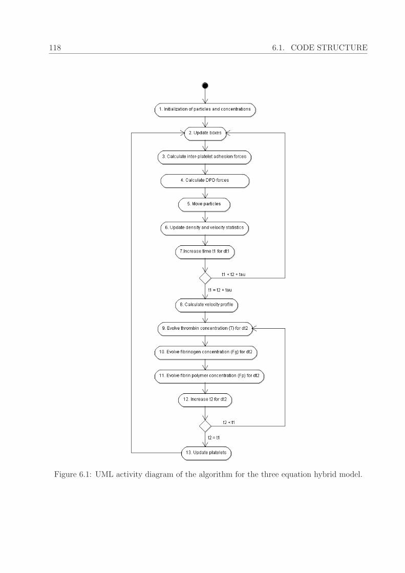
118 6.1. CODE STRUCTURE
Figure 6.1: UML activity diagram of the algorithm for the three equation hybrid model.

6.1. CODE STRUCTURE 119
• CellData. Object of CellData class contains data on a single cell (erythrocyte) mem-brane. The data includes a list of ids of particles that are part of the cell membrane,and supplementary data like the current cell volume. The ids of a particles is definedin the list of all particles. This structure is used in the simulation of an erythrocytemembrane. As no complex model of cells was used in the hybrid models described inChapters 3 and 4, this structure will not be discussed further in this section.
• BoxData. Object of BoxData class encapsulates data related to a single box (seeboxing scheme in Section 6.2.1). It contains an array of particle ids.
• BoxPairData. Object of BoxPairData class contains ids of two neighbouring boxes(see boxing scheme in Section 6.2.1).
• BondData. Object of BondData class contains ids of two connected platelet particlesand a time counter which memorizes the age of the connection.
• StatData. Object of StatData class contains summary data on the number of particlesand their velocities in some small part (or volume) of the simulation domain. The dataon particles in a such volume is summarized through several steps of the DPD part ofthe algorithm, and is afterwards used to calculate density and velocity profiles. After,obtaining the density and velocity profiles, the data is reset.
VelocityData. Object of VelocityData class contains an array of vectors with in-formation on a velocity profile. The velocity profile is obtained by averaging datacontained in a collection of StatData objects.
DensityData. Object of VelocityData class contains an array with information ona density profile. Similarly to the velocity profile, the density profile is obtained byaveraging data contained in a collection of StatData objects.
ProteinData. Object of ProteinData class contains an array with information on aprotein concentration profile.
The objects of classes described above were organized in the following collections:
• Particle list. A collection of ParticleData objects. If possible, it is preferable tostore the ParticleData objects in an array, in order to achieve better simulation per-formance. In that case the id of the particle can be defined as the particle position inthe array. If an array cannot be used because of memory limitations, a list or other,more complex collections, can be used instead. In that case each member of the listcontains ParticleData object and its id. As particles are removed and created in eachstep of the algorithm, the performance when using the array structure can be signifi-cantly reduced. This problem can be solved by using more complex structures whichhave the array structure in its base, but also by using a smarter management of objectinsertions and removals.
• List of boxes. A collection of BoxData objects and their ids. The objects in the list
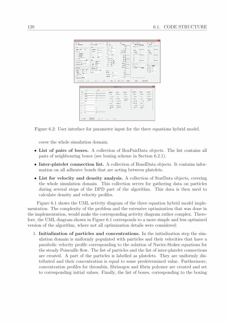
120 6.1. CODE STRUCTURE
Figure 6.2: User interface for parameter input for the three equations hybrid model.
cover the whole simulation domain.
• List of pairs of boxes. A collection of BoxPairData objects. The list contains allpairs of neighbouring boxes (see boxing scheme in Section 6.2.1).
• Inter-platelet connection list. A collection of BondData objects. It contains infor-mation on all adhesive bonds that are acting between platelets.
• List for velocity and density analysis. A collection of StatData objects, coveringthe whole simulation domain. This collection serves for gathering data on particlesduring several steps of the DPD part of the algorithm. This data is then used tocalculate density and velocity profiles.
Figure 6.1 shows the UML activity diagram of the three equation hybrid model imple-mentation. The complexity of the problem and the extensive optimization that was done inthe implementation, would make the corresponding activity diagram rather complex. There-fore, the UML diagram shown in Figure 6.1 corresponds to a more simple and less optimizedversion of the algorithm, where not all optimization details were considered:
1. Initialization of particles and concentrations. In the initialization step the sim-ulation domain is uniformly populated with particles and their velocities that have aparabolic velocity profile corresponding to the solution of Navier-Stokes equations forthe steady Poiseuille flow. The list of particles and the list of inter-platelet connectionsare created. A part of the particles is labelled as platelets. They are uniformly dis-tributed and their concentration is equal to some predetermined value. Furthermore,concentration profiles for thrombin, fibrinogen and fibrin polymer are created and setto corresponding initial values. Finally, the list of boxes, corresponding to the boxing
6.1. CODE STRUCTURE 121
scheme described in Section 6.2.1 is created.
2. Update boxes. Boxes are first emptied, then particles are separated and placed inboxes depending on their positions.
3. Calculate inter-platelet adhesion forces. Adhesion forces are calculated for eachpair of connected platelets. If for any pair of connected platelets, their relative distanceis greater than the critical distance dD (see Section 3.1), the corresponding connectionis removed from the list.
4. Calculate DPD forces. Following the boxing scheme described in Section 6.2.1,for each meaningful pair of boxes (Figure 6.3) DPD forces are calculated between allparticles related to those boxes. If two platelets that are not connected come in physicalcontact, and their relative distance is smaller than the critical distance dC (see Section3.1), a connection between them is created and added to the list of connections.
5. Move particles. Each particle is moved for the corresponding total force acting on itand for the time step dt1. If a particle interacts with the boundaries of the simulationdomain, its position and velocity are adjusted following the rules for a correspondingboundary (see Section 2.3). If the Particle Generation Area is used, the particle canbe removed or added to the particle list. It is removed if it crosses the SA outflowboundary. If it crosses the GA outflow boundary, its copy is added to the particle listinstead. After calculating the particle’s new velocity and position, the force acting onthe particle resets to zero.
6. Update density and velocity statistics. Data for density and velocity profiles areupdated with positions and velocities of particles.
7. Increase time t1 for dt1. A step of the DPD part of the algorithm ends by addingtime step dt1 to the total DPD simulation time t1.
8. Calculate velocity profile. After the DPD part of the algorithm is simulated forsome τ period of time, density and velocity profiles are calculated from data gatheredin the same period of time.
9. Evolve thrombin concentration (T ) for dt2. Thrombin concentration is evolvedfor time step dt2, taking into account the calculated velocity profile.
10. Evolve fibrinogen concentration (Fg) for dt2. Fibrinogen concentration is evolvedfor time step dt2, taking into account the calculated velocity profile and the latestthrombin concentration.
11. Evolve fibrin polymer concentration (Fp) for dt2. Fibrin polymer concentrationis evolved for time step dt2, taking into account the latest fibrinogen concentration.
12. Increase time t2 for dt2. A step of the PDE part of the algorithm ends by addingtime step dt2 to the total DPD simulation time t2.

122 6.2. OPTIMIZATION
13. Update platelets. Once the concentrations have been evolved for τ period of time,the status of platelets is updated. If at the platelet’s position the concentration of fibrinpolymer is larger than the critical concentration cFp the platelet changes its state to“non-adhesive”.
6.2 Optimization
6.2.1 Boxing scheme
Figure 6.3: Boxing scheme: Simulation domain is divided into boxes depending on themaximal radius of inter-particle influence (rc in DPD). Then particles from box Bij are incontact with themselves and with particles from surrounding boxes. The scheme ensuresthat all the other particles are to far away to exert forces on particles in box Bij. Reprintedwith permission from [117] – A. Tosenberger et al., Russian Journal of Numerical Analysisand Mathematical Modelling, De Gruyter, 2012.
In DPD simulations most of the total computational time is spent on the calculations of inter-particle forces, therefore this is the part of the code where optimisation would have the largestimpact. Usually, the cut-off radius of inter-particle force in DPD (rc) is much smaller thanthe sizes of the simulation domain, thus the calculation of forces between all possible pairs ofparticles is very inefficient because most of such pairs have an inter-particle distance largerthan the cut-off radius. In order to avoid as much of such pairs of particles as possible, thesimulation domain, a rectangle in our 2D case, can be divided into smaller rectangles (calledboxes) [18] with lengths of sides equal to min {xεR+|x ≥ rc ∧ ∃nεN such that L = nx} andmin {yεR+|y ≥ rc ∧ ∃nεN such that D = ny}, where L is the length of the domain, and D is
6.2. OPTIMIZATION 123
its height. Construction of a such rectangular subdivision ensures that for each particle p wecan find its corresponding box Bi,j and that all particles which have non-zero inter-particleforce with particle p are contained in the box Bi,j and 8 surrounding boxes. This eliminatesmost of the pairs of particles which have a zero inter-particle force, and therefore drasticallyreduces the computation time. Furthermore, the described domain subdivision enables oneto easily paralellize the process of calculation of inter-particle forces by dividing the set ofall pairs of “connected” boxes into multiple disjunct subsets.
Another possibility to decrease the simulation time it to increase the time step. DPD,due to its definition of the conservative force as a finite function and due to the existenceof dissipating forces, enables a certain increase in the time step compared to other particlemethods like Molecular Dynamics.
6.2.2 Velocity profile smoothing
In hybrid models, described in Chapter 4, the sensitivity of the model on changes in theflow is regulated by the period of data exchange between the discrete and the continuouspart of the model. Reducing this period will increase the frequency of data exchange, thusmaking the model more precise. However, this will also reduce the measurement time forthe velocity profile, and thus cause the increase of noise in the measured profile. This effectof the noise increase can be eliminated to some level by applying methods for noise filteringor smoothing. One of such methods which proved to be efficient for this problem is theGaussian filter. In one dimension the Gaussian filter method consists of convolution of themeasured data f with a normalized Gaussian function g:
(f ∗ g) (x) =∞∫
−∞
f (t) g (x− t) dt, (6.1)
where g is given by
g (x) =1
σ√2π
e−x2
2σ2 . (6.2)
and σ is the standard deviation. In two-dimensions the velocity field can be separated oncomponents of velocity (x- and y-direction velocity profile). Then the Gaussian filter can beapplied on each of the velocity profiles separately. The two dimensional Gaussian functionhas the following form:
g (x, y) =1
2πσ2e−
x2+y2
2σ2 . (6.3)
6.2.3 Dual time steps
In DPD models of platelet aggregation in flow, described in Chapters 3 and 4, the inter-platelet adhesion forces are usually much stronger than DPD inter-particle forces. Because
124 6.2. OPTIMIZATION
of the stronger forces the time step needs to be significantly lower than it would be the casein a simulation without platelet aggregation. As aggregated platelets occupy only a smallpart of the simulation domain, in each step of the algorithm DPD forces between particles inthe rest of the domain are calculated with the unnecessary small time step. A possible wayto avoid this problem and to increase the computational efficiency of the algorithm is to usetwo time steps, instead of only one. The first time step, dtdpd, serves for DPD interactions,while the second one, dtplt, is used for platelet interactions. It is expected that the DPDtime step is significantly larger than the inter-platelet time step (dtdpd � dtplt). In the oneDPD step dtdpd of the algorithm the DPD forces are first calculated between all particles,including platelets. Then, before plasma particles are moved for dtdpd time step, the inter-platelet forces are calculated and only platelets are moved for time step dtplt. Afterwards,the inter-platelet forces are recalculated and platelets are moved for the time step dtplt. Thisprocess is repeated until the sum of dtplt steps is not equal to the dtdpd step. Then the plasmaparticles are moved for dtdpd time step. This approach offers a significant increase in thecomputational performance for simulations of clot growth.
6.2.4 Additional integration scheme for the equations of motionin DPD
In scope of this work a new method was also used. The method can be considered as semi-implicit in the context of the dissipative force, as it takes implicitly a part of the velocityterm into the calculation of the dissipative force. Let us write a sum of DPD forces on someparticle i:
Fi =∑j
(FCij(ri, rj) + FD
ij (ri, rj,vi,vj) + FRij(ri, rj)
). (6.4)
where the conservative and the random force depend only of the positions of the particlesi and j, while the dissipative force depends additionally of particles’ velocities. Let us takethe velocity of the particle i in the implicit form and the remaining variables in the explicitform:
Fi =∑j
(FCij(r
ni , r
nj ) + FD
ij (rni , r
nj ,v
n+1i ,vnj ) + FR
ij(rni , r
nj )). (6.5)
By including it in the first step of Euler integration method (equation (2.8)) the followingequation is obtained :
vn+1i = vni +
dt
mi
∑j
(FCij(r
ni , r
nj ) + FD
ij (rni , r
nj ,v
n+1i ,vnj ) + FR
ij(rni , r
nj )). (6.6)
6.2. OPTIMIZATION 125
After expanding the dissipative force to its full form given by the equation (2.2) andplacing all the expressions multiplying vn+1
i on the left side one obtains:
vn+1i +
dt
m
∑j
γωD(rnij)(vn+1i · rnij)rnij = (6.7)
= vni +dt
mi
∑j
(FCij(r
ni , r
nj ) + γωD(rnij)(v
nj · rnij)rnij + FR
ij(rni , r
nj )),
where rij = ri − rj, rij = |rij| and rij = rij/rij. Now the left side of the equation (6.7) canbe written as:
vn+1i
(I +
dt
m
∑j
γωD(rnij)(rnij ⊗ rnij)
)= (6.8)
= vni +dt
mi
∑j
(FCij(r
ni , r
nj ) + γωD(rnij)(v
nj · rnij)rnij + FR
ij(rni , r
nj )).
Set
A = I +dt
m
∑j
γωD(rnij)(rnij ⊗ rnij). (6.9)
Lemma 6.1. If vi ∈ Rn for i = 1, . . . , k and αi ∈ R , i = 1, . . . , k, such that αi ≥ 0, ∀i,
then the matrix A = I +k∑j=1
αj (vj ⊗ vj) is invertible.
Proof. Let us first define matrices Ai as
Ai = αi (vi ⊗ vi) , for i = 1, . . . k. (6.10)
Let us first note that matrices Ai, i = 1, . . . , k, are symmetric and positive semi-definiteas for any vector x ∈ R
n we have:
xτAix = αi (x1 ... xn)
⎛⎜⎜⎜⎝v21 ... v1vn...
. . ....
vnv1 ... v2n
⎞⎟⎟⎟⎠⎛⎜⎜⎜⎝
x1
...
xn
⎞⎟⎟⎟⎠ (6.11)
= αi
(v1
n∑i=1
xivi ... vn
n∑i=1
xivi
)⎛⎜⎜⎜⎝x1
...
xn
⎞⎟⎟⎟⎠ (6.12)
= αi
n∑j=1
(xjvj
n∑i=1
xivi
)= αi (x1v1 + . . . xnvn)
2 ≥ 0. (6.13)
126 6.2. OPTIMIZATION
As the identity matrix is positive definite and as the sum A + B of a positive definitematrix A and a positive semi-definite matrix B is positive definite:
xτAx > 0, ∀x ∈ Rn, x = 0, (6.14)
xτBx ≥ 0, ∀x ∈ Rn, (6.15)
xτ (A+B)x = (xτA+ xτB)x = xτAx+ xτBx > 0 ∀x ∈ Rn, x = 0, (6.16)
it follows that I +n∑i=1
Ai is a positive definite matrix, and as such is invertible.
From Lemma 6.1 it follows that the matrix A is invertible, so from the equation (6.8)we can write:
vn+1i =
[vni +
dt
mi
∑j
(FCij(r
ni , r
nj ) + γωD(rnij)(v
nj · rnij)rnij + FR
ij(rni , r
nj ))]
A−1. (6.17)
Once the new velocity of particle i is obtained, its new position can be calculated bythe second step of Euler integration method (the equation (2.9)).
On the one hand the previously described method is not symmetrical as one part ofthe velocity difference vi − vj is taken implicitly and the other part explicitly. As a resultthe particle system does not preserve its total momentum. On the other hand, for a smalltime step the error does not significantly influence the behaviour of the whole system, and itallows an increase of time step for the DPD method for several orders of magnitude. Becauseof the loss of symmetry, the method should be used cautiously and results should be verifiedby comparison to a more precise integration scheme.
6.2.5 Parallelism - OpenMP, GPGPU
Dissipative Particle Dynamics, as a discrete particle method allows a certain level of paral-lelism. Different technical solutions can be used in order to use this ability. One of themis multicore computing. A multicore processors consists of multiple execution units, called“cores”, that are placed on the same chip. Each of the cores is capable of executing its ownthread of instructions independently of the other cores, i.e. they can work asynchronously.Multicore processors are today present in most of the personal computers in form of centralprocessing units (CPU). As the software for modelling blood coagulation was developed inC++, one of the most prominent application programming interfaces (API) for paralleliza-tion, called Open Multi-Processing (OMP), was used to run the code in parallel on a CPU.In a single step of the algorithm, especially if using the boxing scheme, the data (particleposition, velocity, state, etc.) is being reused to some extent. However, the reuse of the data
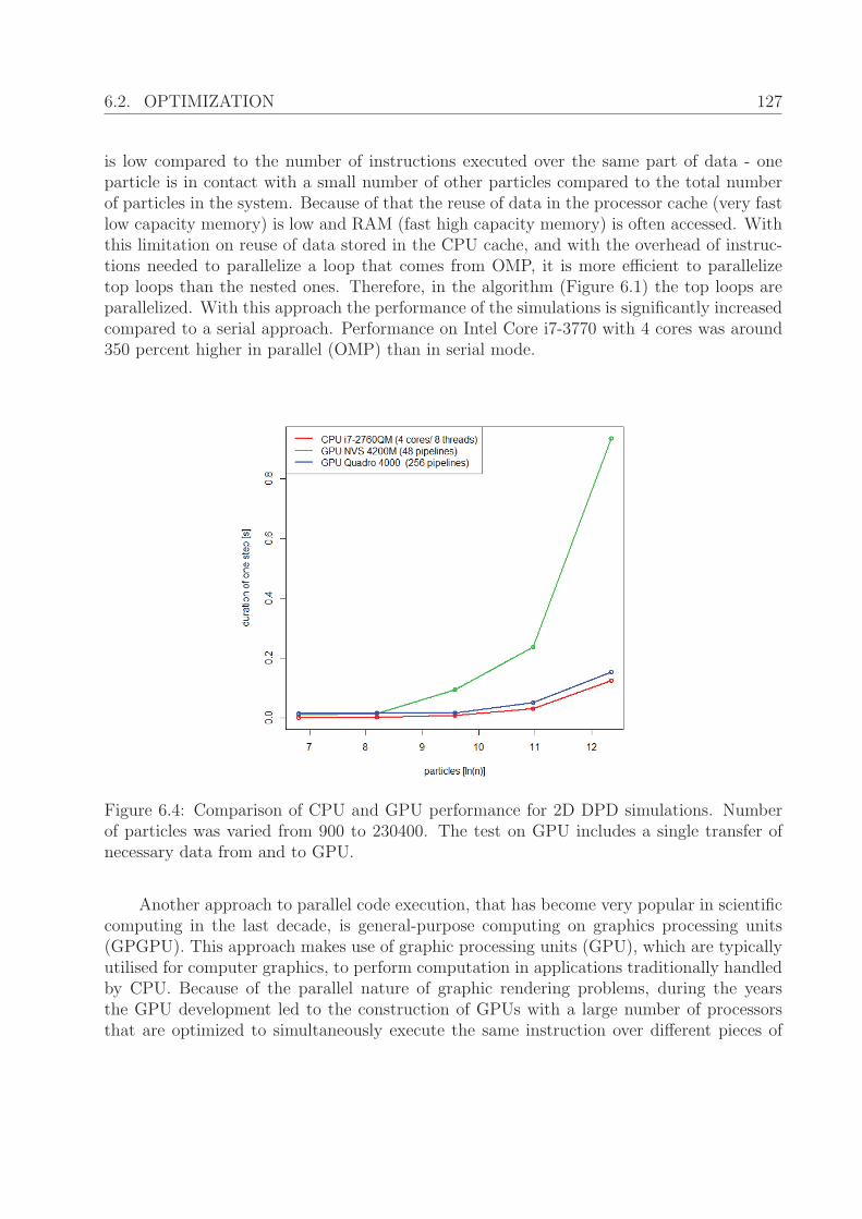
6.2. OPTIMIZATION 127
is low compared to the number of instructions executed over the same part of data - oneparticle is in contact with a small number of other particles compared to the total numberof particles in the system. Because of that the reuse of data in the processor cache (very fastlow capacity memory) is low and RAM (fast high capacity memory) is often accessed. Withthis limitation on reuse of data stored in the CPU cache, and with the overhead of instruc-tions needed to parallelize a loop that comes from OMP, it is more efficient to parallelizetop loops than the nested ones. Therefore, in the algorithm (Figure 6.1) the top loops areparallelized. With this approach the performance of the simulations is significantly increasedcompared to a serial approach. Performance on Intel Core i7-3770 with 4 cores was around350 percent higher in parallel (OMP) than in serial mode.
Figure 6.4: Comparison of CPU and GPU performance for 2D DPD simulations. Numberof particles was varied from 900 to 230400. The test on GPU includes a single transfer ofnecessary data from and to GPU.
Another approach to parallel code execution, that has become very popular in scientificcomputing in the last decade, is general-purpose computing on graphics processing units(GPGPU). This approach makes use of graphic processing units (GPU), which are typicallyutilised for computer graphics, to perform computation in applications traditionally handledby CPU. Because of the parallel nature of graphic rendering problems, during the yearsthe GPU development led to the construction of GPUs with a large number of processorsthat are optimized to simultaneously execute the same instruction over different pieces of
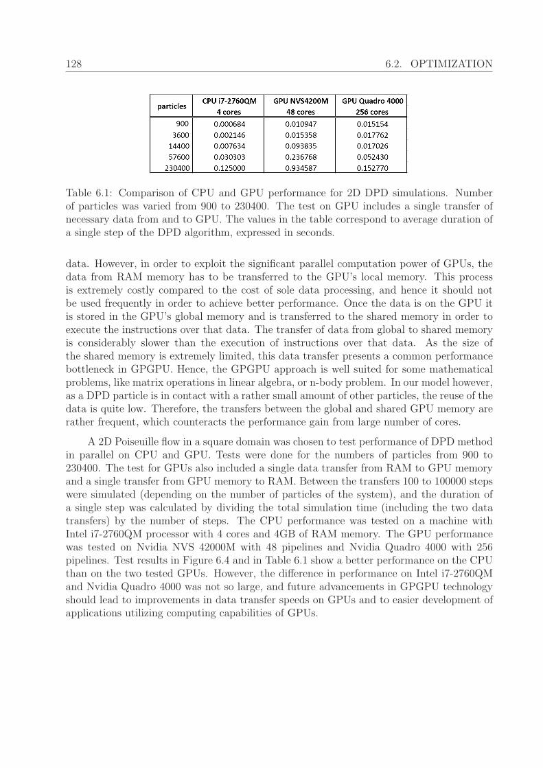
128 6.2. OPTIMIZATION
Table 6.1: Comparison of CPU and GPU performance for 2D DPD simulations. Numberof particles was varied from 900 to 230400. The test on GPU includes a single transfer ofnecessary data from and to GPU. The values in the table correspond to average duration ofa single step of the DPD algorithm, expressed in seconds.
data. However, in order to exploit the significant parallel computation power of GPUs, thedata from RAM memory has to be transferred to the GPU’s local memory. This processis extremely costly compared to the cost of sole data processing, and hence it should notbe used frequently in order to achieve better performance. Once the data is on the GPU itis stored in the GPU’s global memory and is transferred to the shared memory in order toexecute the instructions over that data. The transfer of data from global to shared memoryis considerably slower than the execution of instructions over that data. As the size ofthe shared memory is extremely limited, this data transfer presents a common performancebottleneck in GPGPU. Hence, the GPGPU approach is well suited for some mathematicalproblems, like matrix operations in linear algebra, or n-body problem. In our model however,as a DPD particle is in contact with a rather small amount of other particles, the reuse of thedata is quite low. Therefore, the transfers between the global and shared GPU memory arerather frequent, which counteracts the performance gain from large number of cores.
A 2D Poiseuille flow in a square domain was chosen to test performance of DPD methodin parallel on CPU and GPU. Tests were done for the numbers of particles from 900 to230400. The test for GPUs also included a single data transfer from RAM to GPU memoryand a single transfer from GPU memory to RAM. Between the transfers 100 to 100000 stepswere simulated (depending on the number of particles of the system), and the duration ofa single step was calculated by dividing the total simulation time (including the two datatransfers) by the number of steps. The CPU performance was tested on a machine withIntel i7-2760QM processor with 4 cores and 4GB of RAM memory. The GPU performancewas tested on Nvidia NVS 42000M with 48 pipelines and Nvidia Quadro 4000 with 256pipelines. Test results in Figure 6.4 and in Table 6.1 show a better performance on the CPUthan on the two tested GPUs. However, the difference in performance on Intel i7-2760QMand Nvidia Quadro 4000 was not so large, and future advancements in GPGPU technologyshould lead to improvements in data transfer speeds on GPUs and to easier development ofapplications utilizing computing capabilities of GPUs.
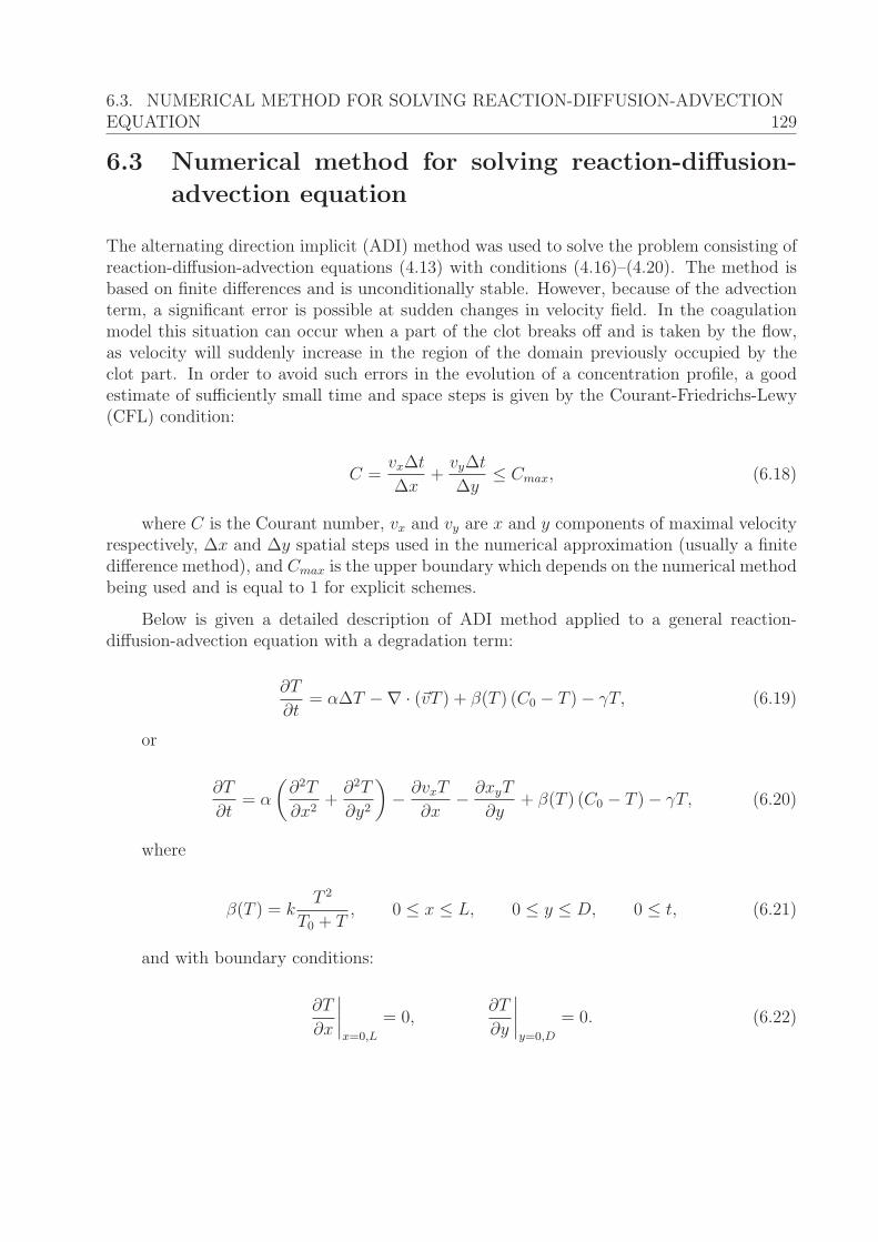
6.3. NUMERICAL METHOD FOR SOLVING REACTION-DIFFUSION-ADVECTIONEQUATION 129
6.3 Numerical method for solving reaction-diffusion-
advection equation
The alternating direction implicit (ADI) method was used to solve the problem consisting ofreaction-diffusion-advection equations (4.13) with conditions (4.16)–(4.20). The method isbased on finite differences and is unconditionally stable. However, because of the advectionterm, a significant error is possible at sudden changes in velocity field. In the coagulationmodel this situation can occur when a part of the clot breaks off and is taken by the flow,as velocity will suddenly increase in the region of the domain previously occupied by theclot part. In order to avoid such errors in the evolution of a concentration profile, a goodestimate of sufficiently small time and space steps is given by the Courant-Friedrichs-Lewy(CFL) condition:
C =vxΔt
Δx+
vyΔt
Δy≤ Cmax, (6.18)
where C is the Courant number, vx and vy are x and y components of maximal velocityrespectively, Δx and Δy spatial steps used in the numerical approximation (usually a finitedifference method), and Cmax is the upper boundary which depends on the numerical methodbeing used and is equal to 1 for explicit schemes.
Below is given a detailed description of ADI method applied to a general reaction-diffusion-advection equation with a degradation term:
∂T
∂t= αΔT −∇ · (�vT ) + β(T ) (C0 − T )− γT, (6.19)
or
∂T
∂t= α
(∂2T
∂x2+
∂2T
∂y2
)− ∂vxT
∂x− ∂xyT
∂y+ β(T ) (C0 − T )− γT, (6.20)
where
β(T ) = kT 2
T0 + T, 0 ≤ x ≤ L, 0 ≤ y ≤ D, 0 ≤ t, (6.21)
and with boundary conditions:
∂T
∂x
∣∣∣∣x=0,L
= 0,∂T
∂y
∣∣∣∣y=0,D
= 0. (6.22)
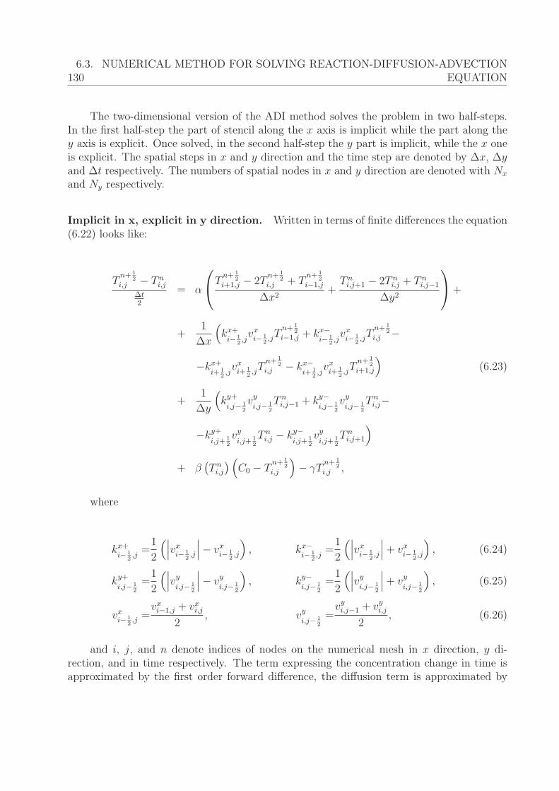
1306.3. NUMERICAL METHOD FOR SOLVING REACTION-DIFFUSION-ADVECTION
EQUATION
The two-dimensional version of the ADI method solves the problem in two half-steps.In the first half-step the part of stencil along the x axis is implicit while the part along they axis is explicit. Once solved, in the second half-step the y part is implicit, while the x oneis explicit. The spatial steps in x and y direction and the time step are denoted by Δx, Δyand Δt respectively. The numbers of spatial nodes in x and y direction are denoted with Nx
and Ny respectively.
Implicit in x, explicit in y direction. Written in terms of finite differences the equation(6.22) looks like:
Tn+ 1
2i,j − T n
i,j
Δt2
= α
⎛⎝Tn+ 1
2i+1,j − 2T
n+ 12
i,j + Tn+ 1
2i−1,j
Δx2+
T ni,j+1 − 2T n
i,j + T ni,j−1
Δy2
⎞⎠+
+1
Δx
(kx+i− 1
2,jvxi− 1
2,jTn+ 1
2i−1,j + kx−
i− 12,jvxi− 1
2,jTn+ 1
2i,j −
−kx+i+ 1
2,jvxi+ 1
2,jTn+ 1
2i,j − kx−
i+ 12,jvxi+ 1
2,jTn+ 1
2i+1,j
)(6.23)
+1
Δy
(ky+i,j− 1
2
vyi,j− 1
2
T ni,j−1 + ky−
i,j− 12
vyi,j− 1
2
T ni,j−
−ky+i,j+ 1
2
vyi,j+ 1
2
T ni,j − ky−
i,j+ 12
vyi,j+ 1
2
T ni,j+1
)+ β
(T ni,j
) (C0 − T
n+ 12
i,j
)− γT
n+ 12
i,j ,
where
kx+i− 1
2,j=1
2
(∣∣∣vxi− 12,j
∣∣∣− vxi− 1
2,j
), kx−
i− 12,j=1
2
(∣∣∣vxi− 12,j
∣∣∣+ vxi− 1
2,j
), (6.24)
ky+i,j− 1
2
=1
2
(∣∣∣vyi,j− 1
2
∣∣∣− vyi,j− 1
2
), ky−
i,j− 12
=1
2
(∣∣∣vyi,j− 1
2
∣∣∣+ vyi,j− 1
2
), (6.25)
vxi− 1
2,j=vxi−1,j + vxi,j
2, vy
i,j− 12
=vyi,j−1 + vyi,j
2, (6.26)
and i, j, and n denote indices of nodes on the numerical mesh in x direction, y di-rection, and in time respectively. The term expressing the concentration change in time isapproximated by the first order forward difference, the diffusion term is approximated by
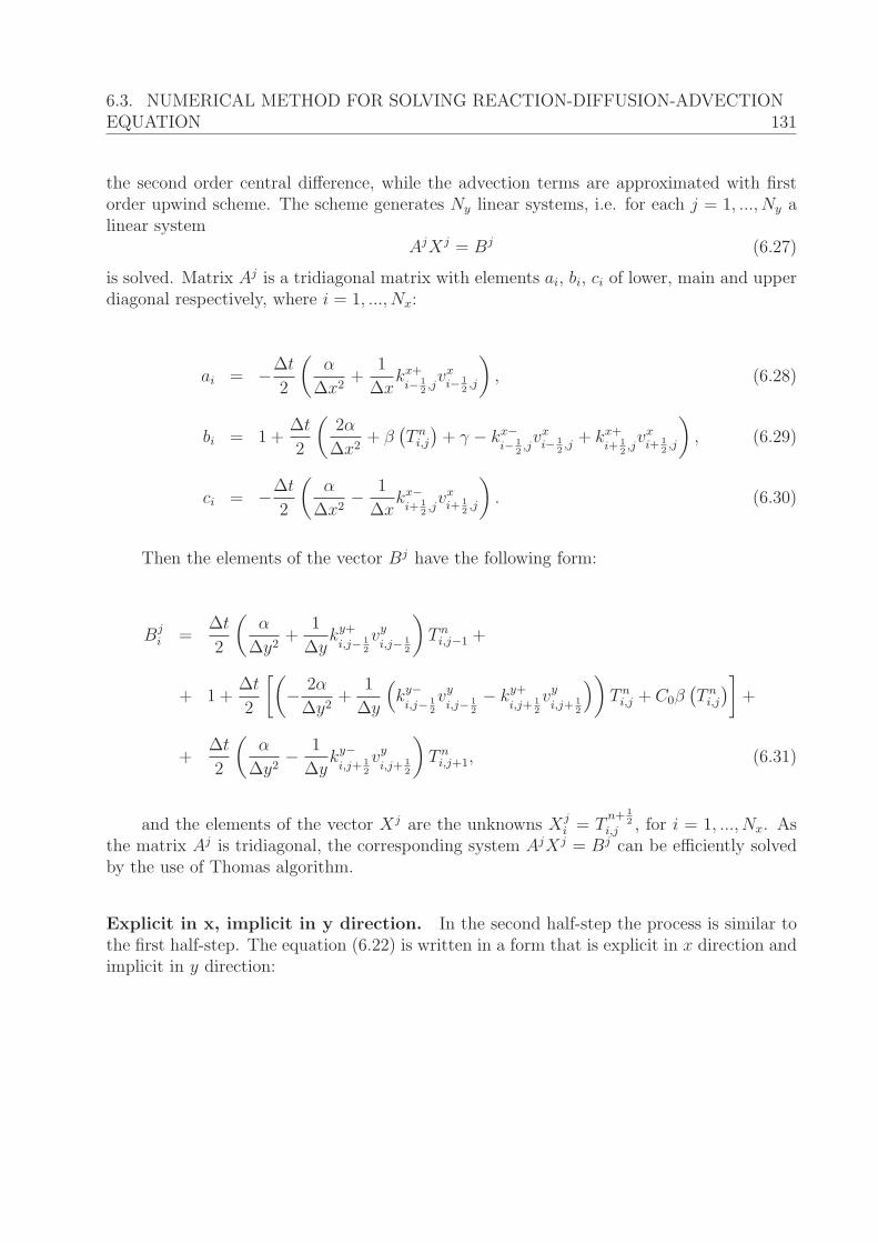
6.3. NUMERICAL METHOD FOR SOLVING REACTION-DIFFUSION-ADVECTIONEQUATION 131
the second order central difference, while the advection terms are approximated with firstorder upwind scheme. The scheme generates Ny linear systems, i.e. for each j = 1, ..., Ny alinear system
AjXj = Bj (6.27)
is solved. Matrix Aj is a tridiagonal matrix with elements ai, bi, ci of lower, main and upperdiagonal respectively, where i = 1, ..., Nx:
ai = −Δt
2
(α
Δx2+
1
Δxkx+i− 1
2,jvxi− 1
2,j
), (6.28)
bi = 1 +Δt
2
(2α
Δx2+ β
(T ni,j
)+ γ − kx−
i− 12,jvxi− 1
2,j+ kx+
i+ 12,jvxi+ 1
2,j
), (6.29)
ci = −Δt
2
(α
Δx2− 1
Δxkx−i+ 1
2,jvxi+ 1
2,j
). (6.30)
Then the elements of the vector Bj have the following form:
Bji =
Δt
2
(α
Δy2+
1
Δyky+i,j− 1
2
vyi,j− 1
2
)T ni,j−1 +
+ 1 +Δt
2
[(− 2α
Δy2+
1
Δy
(ky−i,j− 1
2
vyi,j− 1
2
− ky+i,j+ 1
2
vyi,j+ 1
2
))T ni,j + C0β
(T ni,j
)]+
+Δt
2
(α
Δy2− 1
Δyky−i,j+ 1
2
vyi,j+ 1
2
)T ni,j+1, (6.31)
and the elements of the vector Xj are the unknowns Xji = T
n+ 12
i,j , for i = 1, ..., Nx. Asthe matrix Aj is tridiagonal, the corresponding system AjXj = Bj can be efficiently solvedby the use of Thomas algorithm.
Explicit in x, implicit in y direction. In the second half-step the process is similar tothe first half-step. The equation (6.22) is written in a form that is explicit in x direction andimplicit in y direction:
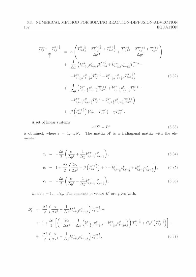
1326.3. NUMERICAL METHOD FOR SOLVING REACTION-DIFFUSION-ADVECTION
EQUATION
T n+1i,j − T
n+ 12
i,j
Δt2
= α
⎛⎝Tn+ 1
2i+1,j − 2T
n+ 12
i,j + Tn+ 1
2i−1,j
Δx2+
T n+1i,j+1 − 2T n+1
i,j + T n+1i,j−1
Δy2
⎞⎠+
1
Δx
(kx+i− 1
2,jvxi− 1
2,jTn+ 1
2i−1,j + kx−
i− 12,jvxi− 1
2,jTn+ 1
2i,j −
−kx+i+ 1
2,jvxi+ 1
2,jTn+ 1
2i,j − kx−
i+ 12,jvxi+ 1
2,jTn+ 1
2i+1,j
)(6.32)
+1
Δy
(ky+i,j− 1
2
vyi,j− 1
2
T n+1i,j−1 + ky−
i,j− 12
vyi,j− 1
2
T n+1i,j −
−ky+i,j+ 1
2
vyi,j+ 1
2
T n+1i,j − ky−
i,j+ 12
vyi,j+ 1
2
T n+1i,j+1
)+ β
(Tn+ 1
2i,j
) (C0 − T n+1
i,j
)− γT n+1i,j .
A set of linear systemsAiX i = Bi (6.33)
is obtained, where i = 1, ..., Nx. The matrix Ai is a tridiagonal matrix with the ele-ments:
ai = −Δt
2
(α
Δy2+
1
Δyky+i,j− 1
2
vyi,j− 1
2
), (6.34)
bi = 1 +Δt
2
(2α
Δy2+ β
(Tn+ 1
2i,j
)+ γ − ky−
i,j− 12
vyi,j− 1
2
+ ky+i,j+ 1
2
vyi,j+ 1
2
), (6.35)
ci = −Δt
2
(α
Δy2− 1
Δyky−i,j+ 1
2
vyi,j+ 1
2
). (6.36)
where j = 1, ..., Ny. The elements of vector Bi are given with:
Bij =
Δt
2
(α
Δx2+
1
Δxkx+i− 1
2,jvxi− 1
2,j
)Tn+ 1
2i−1,j +
+ 1 +Δt
2
[(− 2α
Δx2+
1
Δx
(kx−i− 1
2,jvxi− 1
2,j− kx+
i+ 12,jvxi+ 1
2,j
))Tn+ 1
2i,j + C0β
(Tn+ 1
2i,j
)]+
+Δt
2
(α
Δx2− 1
Δxkx−i+ 1
2,jvxi+ 1
2,j
)Tn+ 1
2i+1,j, (6.37)
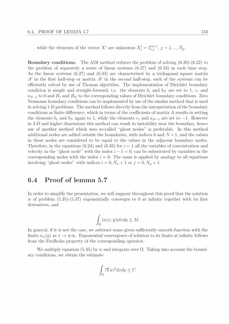
6.4. PROOF OF LEMMA 5.7 133
while the elements of the vector X i are unknowns X ij = T n+1
i,j , j = 1, ..., Ny.
Boundary conditions. The ADI method reduces the problem of solving (6.20)-(6.22) tothe problem of separately a series of linear systems (6.27) and (6.33) in each time step.As the linear systems (6.27) and (6.33) are characterised by a tridiagonal square matrixAi in the first half-step or matrix Aj in the second half-step, each of the systems can beefficiently solved by use of Thomas algorithm. The implementation of Dirichlet boundarycondition is simple and straight-forward, i.e. the elements b1 and bN are set to 1, c1 andaN−1 to 0 and B1 and BN to the corresponding values of Dirichlet boundary conditions. ZeroNeumann boundary conditions can be implemented by use of the similar method that is usedin solving 1-D problems. The method follows directly from the interpretation of the boundaryconditions as finite difference, which in terms of the coefficients of matrix A results in settingthe elements b1 and bN again to 1, while the elements c1 and aN−1 are set to −1. Howeverin 2-D and higher dimensions this method can result in instability near the boundary, henceuse of another method which uses so-called “ghost nodes” is preferable. In this methodadditional nodes are added outside the boundaries, with indices 0 and N +1, and the valuesin these nodes are considered to be equal to the values in the adjacent boundary nodes.Therefore, in the equations (6.24) and (6.33) for i = 1 all the variables of concentration andvelocity in the “ghost node” with the index i− 1 = 0, can be substituted by variables in thecorresponding nodes with the index i = 0. The same is applied by analogy to all equationsinvolving “ghost nodes” with indices i = 0, Nx + 1 or j = 0, Ny + 1.
6.4 Proof of lemma 5.7
In order to simplify the presentation, we will suppose throughout this proof that the solutionw of problem (5.35)-(5.37) exponentially converges to 0 at infinity together with its firstderivatives, and
∫Ω
|w(x, y)|dxdy ≤ M.
In general, if it is not the case, we subtract some given sufficiently smooth function with thelimits u±(y) as x → ±∞. Exponential convergence of solution to its limits at infinity followsfrom the Fredholm property of the corresponding operator.
We multiply equation (5.35) by w and integrate over Ω. Taking into account the bound-ary conditions, we obtain the estimate
∫Ω
|∇w|2dxdy ≤ C.

134 6.4. PROOF OF LEMMA 5.7
Here and below we denote by C any constant which depends only on K, M and c. Hence∂w/∂y ∈ L2(Ω).
Set v = ∂w/∂y. Then this function satisfies the problem
Δv + c∂v
∂x+ f ′
τ (w)v = 0, (6.38)
y = 0 : v = 0, y = 1 : v = gτ (w). (6.39)
Here and below f ′τ and g′τ denotes the derivatives of these functions with respect to w. Put
φ = f ′τ (w)v and consider the auxiliary problems
Δv± + c∂v±∂x
+ φ = 0, (6.40)
y = 0 : v± = 0, y = 1 : v± = ±K. (6.41)
Then from the maximum principle
v−(x, y) ≤ v(x, y) ≤ v+(x, y), (x, y) ∈ Ω.
Since the function f ′τ (w) is bounded, then φ ∈ L2(Ω). Therefore problems (6.40), (6.41)
are solvable in H2(Ω), and their norms depend only on K, M and c. By virtue of embed-ding theorems (on bounded subsets), the functions v±(x, y) are bounded and, consequently,solution v of problem (6.38), (6.39) admits the estimate:
sup(x,y)∈Ω
|v(x, y)| ≤ C. (6.42)
Next, we multiply equation (6.38) by v and integrate over Ω. Taking into account that v = 0at y = 0 and
∂v
∂y= g′τ (w)gτ (w), y = 1,
we obtain the estimate
∫Ω
|∇v(x, y)|2dxdy ≤ C. (6.43)
Hence ∂v/∂y ∈ L2(Ω).
Set z = ∂v/∂y. Then this function satisfies the equation
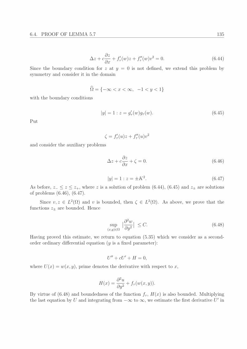
6.4. PROOF OF LEMMA 5.7 135
Δz + c∂z
∂x+ f ′
τ (w)z + f ′′τ (w)v
2 = 0. (6.44)
Since the boundary condition for z at y = 0 is not defined, we extend this problem bysymmetry and consider it in the domain
Ω = {−∞ < x < ∞, −1 < y < 1}with the boundary conditions
|y| = 1 : z = g′τ (w)gτ (w). (6.45)
Put
ζ = f ′τ (u)z + f ′′
τ (u)v2
and consider the auxiliary problems
Δz + c∂z
∂x+ ζ = 0. (6.46)
|y| = 1 : z = ±K2. (6.47)
As before, z− ≤ z ≤ z+, where z is a solution of problem (6.44), (6.45) and z± are solutionsof problems (6.46), (6.47).
Since v, z ∈ L2(Ω) and v is bounded, then ζ ∈ L2(Ω). As above, we prove that thefunctions z± are bounded. Hence
sup(x,y)∈Ω
∣∣∂2w
∂y2∣∣ ≤ C. (6.48)
Having proved this estimate, we return to equation (5.35) which we consider as a second-order ordinary differential equation (y is a fixed parameter):
U ′′ + cU ′ +H = 0,
where U(x) = w(x, y), prime denotes the derivative with respect to x,
H(x) =∂2u
∂y2+ fτ (w(x, y)).
By virtue of (6.48) and boundedness of the function fτ , H(x) is also bounded. Multiplyingthe last equation by U and integrating from −∞ to ∞, we estimate the first derivative U ′ in
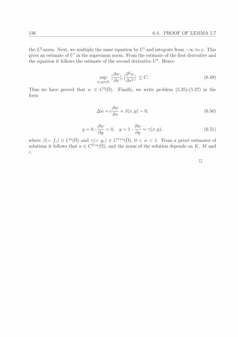
136 6.4. PROOF OF LEMMA 5.7
the L2-norm. Next, we multiply the same equation by U ′ and integrate from −∞ to x. Thisgives an estimate of U ′ in the supremum norm. From the estimate of the first derivative andthe equation it follows the estimate of the second derivative U ′′. Hence
sup(x,y)∈Ω
∣∣∂w∂x
∣∣, ∣∣∂2w
∂x2
∣∣ ≤ C. (6.49)
Thus we have proved that w ∈ C2(Ω). Finally, we write problem (5.35)-(5.37) in theform
Δw + c∂w
∂x+ β(x, y) = 0, (6.50)
y = 0 :∂w
∂y= 0, y = 1 :
∂w
∂y= γ(x, y), (6.51)
where β(= fτ ) ∈ Cα(Ω) and γ(= gτ ) ∈ C1+α(Ω), 0 < α < 1. From a priori estimates ofsolutions it follows that u ∈ C2+α(Ω), and the norm of the solution depends on K, M andc.
�
Related Documents


![Abnormalities of Blood Coagulation[1]](https://static.cupdf.com/doc/110x72/577cce2b1a28ab9e788d80ee/abnormalities-of-blood-coagulation1.jpg)