BIOST 536 Lecture 12 1 Lecture 12 – Introduction to Matching.

BIOST 536 Lecture 12 1

Lecture 12 – Introduction to MatchingMatching/Stratification

Group subjects into subsets on the basis of assumed confounders (e.g. age, gender, clinic, etc)

Matching variables should not be of direct scientific interest

Matching

Done in advance, often in a specified ratio: 1 case to 1 control ; or 1 case to m controls

May be matched on underlying relationship that cannot be quantified (twins, siblings, neighbors)

Stratification

Usually done after data collection on the basis of recorded covariates

Little control over the number of cases and controls in each stratum

n j cases matched to m j controls in stratum j

Strata with either no cases or no controls get eliminated from the analysis

Matched analyzed as stratified

Suppose we match a 40-44 year old case with four 40-44 year old controls, then match another 40-44

year old case with four different 40-44 year old controls

Combine all together and analyze as two cases matched to eight controls (“frequency matching”)

BIOST 536 Lecture 12 2

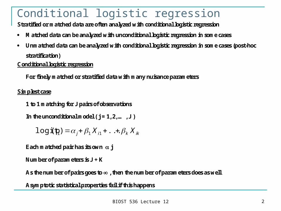
Conditional logistic regressionStratified or matched data are often analyzed with conditional logistic regression

Matched data can be analyzed with unconditional logistic regression in some cases

Unmatched data can be analyzed with conditional logistic regression in some cases (post-hoc

stratification)

Conditional logistic regression

For finely matched or stratified data with many nuisance parameters

Simplest case

1 to 1 matching for J pairs of observations

In the unconditional model ( j = 1, 2, … , J )

ikkij XX ...)(plogit 11i

Each matched pair has its own j

Number of parameters is J + K

As the number of pairs goes to , then the number of parameters does as well

Asymptotic statistical properties fail if this happens

BIOST 536 Lecture 12 3

Conditional logistic regression

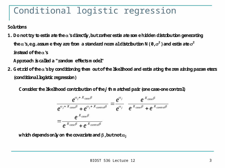
Solutions

1. Do not try to estimate the 's directly, but rather estimate some hidden distribution generating

the 's, e.g. assume they are from a standard normal distribution N( 0, 2 ) and estimate 2

instead of the 's

Approach is called a "random effects model"

2. Get rid of the 's by conditioning them out of the likelihood and estimating the remaining parameters

(conditional logistic regression)

Consider the likelihood contribution of the j th matched pair (one case-one control)

controlcase

case

controlcase

case

j

j

controljcasej

casej

XX

X

XX

X

XX

X

ee

e

ee

e

e

e

ee

e

which depends only on the covariate and , but not j

BIOST 536 Lecture 12 4

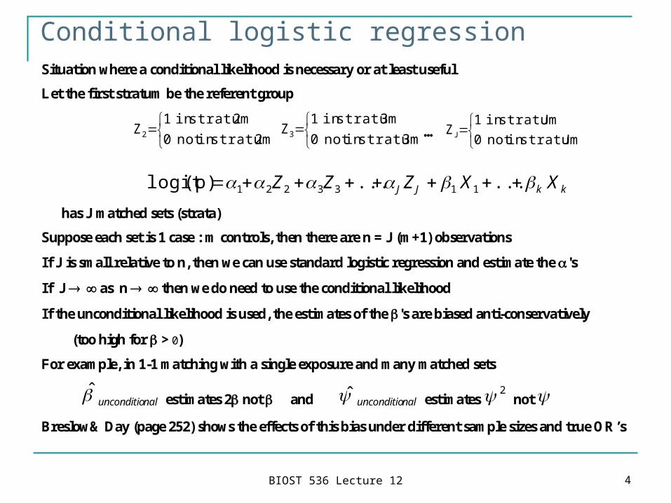
Conditional logistic regressionSituation where a conditional likelihood is necessary or at least useful

Let the first stratum be the referent group

2 stratumin not 0

2 stratumin 1Z2

3 stratumin not 0

3 stratumin 1Z3 …

J stratumin not 0

J stratumin 1ZJ

kkJJ XXZZZ ......(p)logit 1133221

has J matched sets (strata)

Suppose each set is 1 case : m controls, then there are n = J (m+1) observations

If J is small relative to n, then we can use standard logistic regression and estimate the 's

If J as n then we do need to use the conditional likelihood

If the unconditional likelihood is used, the estimates of the 's are biased anti-conservatively

(too high for > 0)

For example, in 1-1 matching with a single exposure and many matched sets

nalunconditio estimates 2 not and nalunconditio estimates 2 not

Breslow& Day (page 252) shows the effects of this bias under different sample sizes and true OR’s

BIOST 536 Lecture 12 5

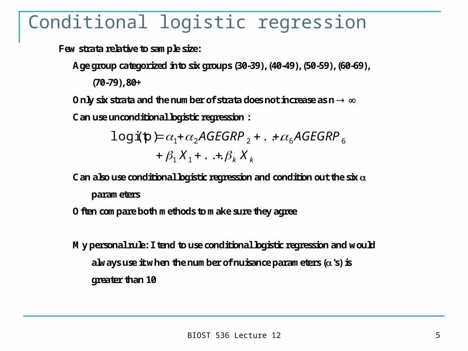
Conditional logistic regressionFew strata relative to sample size:

Age group categorized into six groups (30-39), (40-49), (50-59), (60-69),

(70-79), 80+

Only six strata and the number of strata does not increase as n

Can use unconditional logistic regression :

kk XX

AGEGRPAGEGRP

...

...(p)logit

11

66221

Can also use conditional logistic regression and condition out the six

parameters

Often compare both methods to make sure they agree

My personal rule: I tend to use conditional logistic regression and would

always use it when the number of nuisance parameters ('s) is

greater than 10

BIOST 536 Lecture 12 6

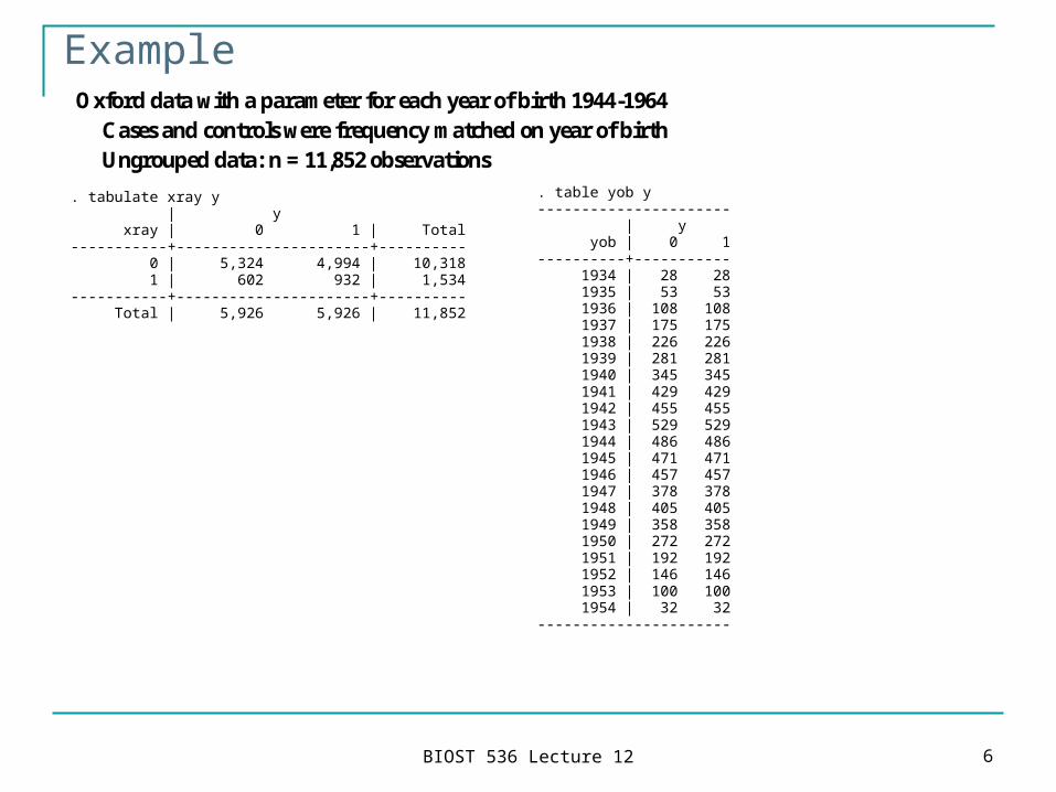
Example Oxford data with a parameter for each year of birth 1944-1964

Cases and controls were frequency matched on year of birth Ungrouped data: n = 11,852 observations

. tabulate xray y | y xray | 0 1 | Total -----------+----------------------+---------- 0 | 5,324 4,994 | 10,318 1 | 602 932 | 1,534 -----------+----------------------+---------- Total | 5,926 5,926 | 11,852

. table yob y ---------------------- | y yob | 0 1 ----------+----------- 1934 | 28 28 1935 | 53 53 1936 | 108 108 1937 | 175 175 1938 | 226 226 1939 | 281 281 1940 | 345 345 1941 | 429 429 1942 | 455 455 1943 | 529 529 1944 | 486 486 1945 | 471 471 1946 | 457 457 1947 | 378 378 1948 | 405 405 1949 | 358 358 1950 | 272 272 1951 | 192 192 1952 | 146 146 1953 | 100 100 1954 | 32 32 ----------------------

BIOST 536 Lecture 12 7

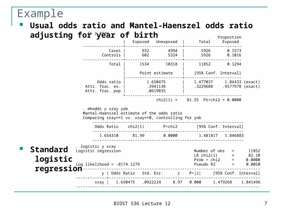
Example Usual odds ratio and Mantel-Haenszel odds ratio adjusting for

year of birth

Standard logistic regression

. cc y xray Proportion | Exposed Unexposed | Total Exposed -----------------+------------------------+------------------------ Cases | 932 4994 | 5926 0.1573 Controls | 602 5324 | 5926 0.1016 -----------------+------------------------+------------------------ Total | 1534 10318 | 11852 0.1294 | | | Point estimate | [95% Conf. Interval] |------------------------+------------------------ Odds ratio | 1.650475 | 1.477037 1.84433 (exact) Attr. frac. ex. | .3941138 | .3229688 .4577978 (exact) Attr. frac. pop | .0619835 | +------------------------------------------------- chi2(1) = 81.55 Pr>chi2 = 0.0000 . mhodds y xray yob Mantel-Haenszel estimate of the odds ratio Comparing xray==1 vs. xray==0, controlling for yob ---------------------------------------------------------------- Odds Ratio chi2(1) P>chi2 [95% Conf. Interval] ---------------------------------------------------------------- 1.654310 81.99 0.0000 1.481817 1.846883 ---------------------------------------------------------------- . logistic y xray

Logistic regression Number of obs = 11852 LR chi2(1) = 82.10 Prob > chi2 = 0.0000 Log likelihood = -8174.1279 Pseudo R2 = 0.0050 ------------------------------------------------------------------------------ y | Odds Ratio Std. Err. z P>|z| [95% Conf. Interval] -------------+---------------------------------------------------------------- xray | 1.650475 .0922224 8.97 0.000 1.479268 1.841496 ------------------------------------------------------------------------------

BIOST 536 Lecture 12 8

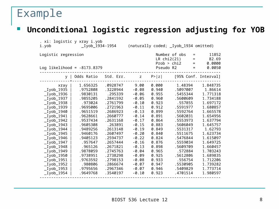
Example Unconditional logistic regression adjusting for YOB

. xi: logistic y xray i.yob i.yob _Iyob_1934-1954 (naturally coded; _Iyob_1934 omitted) Logistic regression Number of obs = 11852 LR chi2(21) = 82.69 Prob > chi2 = 0.0000 Log likelihood = -8173.8379 Pseudo R2 = 0.0050 ------------------------------------------------------------------------------ y | Odds Ratio Std. Err. z P>|z| [95% Conf. Interval] -------------+---------------------------------------------------------------- xray | 1.656325 .0928747 9.00 0.000 1.48394 1.848735 _Iyob_1935 | .9752808 .3228944 -0.08 0.940 .5097007 1.86614 _Iyob_1936 | .9830131 .295339 -0.06 0.955 .5455344 1.771318 _Iyob_1937 | .9855205 .2841592 -0.05 0.960 .5600609 1.734188 _Iyob_1938 | .973024 .2761799 -0.10 0.923 .557855 1.697172 _Iyob_1939 | .9695006 .2721963 -0.11 0.912 .5591977 1.680857 _Iyob_1940 | .9651519 .2686923 -0.13 0.899 .5592764 1.665578 _Iyob_1941 | .9628661 .2660777 -0.14 0.891 .5602031 1.654956 _Iyob_1942 | .9537434 .2631168 -0.17 0.864 .5553973 1.637794 _Iyob_1943 | .9605308 .263891 -0.15 0.883 .5606049 1.645757 _Iyob_1944 | .9489256 .2613148 -0.19 0.849 .5531317 1.62793 _Iyob_1945 | .9460176 .2607497 -0.20 0.840 .5511675 1.623734 _Iyob_1946 | .9405123 .2594737 -0.22 0.824 .5476844 1.615097 _Iyob_1947 | .957647 .2657444 -0.16 0.876 .5559034 1.649725 _Iyob_1948 | .965126 .2671821 -0.13 0.898 .5609709 1.660457 _Iyob_1949 | .9878059 .2745763 -0.04 0.965 .572884 1.703243 _Iyob_1950 | .9738951 .2738298 -0.09 0.925 .5612806 1.689835 _Iyob_1951 | .9763592 .2798153 -0.08 0.933 .556754 1.712206 _Iyob_1952 | .980806 .2866674 -0.07 0.947 .5530905 1.739282 _Iyob_1953 | .9795656 .2967346 -0.07 0.946 .5409829 1.773714 _Iyob_1954 | .9649768 .3540197 -0.10 0.923 .4701514 1.980597 ------------------------------------------------------------------------------

BIOST 536 Lecture 12 9

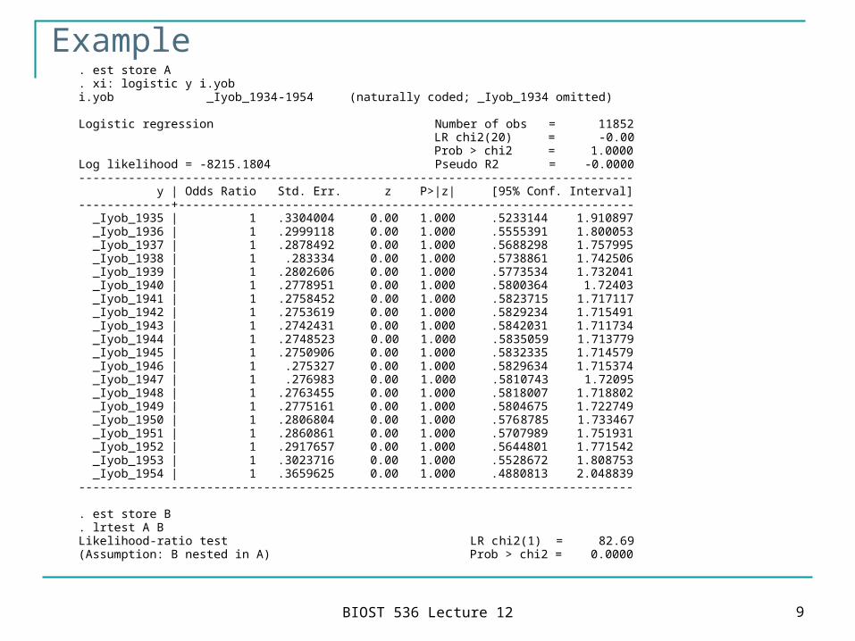
Example. est store A . xi: logistic y i.yob i.yob _Iyob_1934-1954 (naturally coded; _Iyob_1934 omitted) Logistic regression Number of obs = 11852 LR chi2(20) = -0.00 Prob > chi2 = 1.0000 Log likelihood = -8215.1804 Pseudo R2 = -0.0000 ------------------------------------------------------------------------------ y | Odds Ratio Std. Err. z P>|z| [95% Conf. Interval] -------------+---------------------------------------------------------------- _Iyob_1935 | 1 .3304004 0.00 1.000 .5233144 1.910897 _Iyob_1936 | 1 .2999118 0.00 1.000 .5555391 1.800053 _Iyob_1937 | 1 .2878492 0.00 1.000 .5688298 1.757995 _Iyob_1938 | 1 .283334 0.00 1.000 .5738861 1.742506 _Iyob_1939 | 1 .2802606 0.00 1.000 .5773534 1.732041 _Iyob_1940 | 1 .2778951 0.00 1.000 .5800364 1.72403 _Iyob_1941 | 1 .2758452 0.00 1.000 .5823715 1.717117 _Iyob_1942 | 1 .2753619 0.00 1.000 .5829234 1.715491 _Iyob_1943 | 1 .2742431 0.00 1.000 .5842031 1.711734 _Iyob_1944 | 1 .2748523 0.00 1.000 .5835059 1.713779 _Iyob_1945 | 1 .2750906 0.00 1.000 .5832335 1.714579 _Iyob_1946 | 1 .275327 0.00 1.000 .5829634 1.715374 _Iyob_1947 | 1 .276983 0.00 1.000 .5810743 1.72095 _Iyob_1948 | 1 .2763455 0.00 1.000 .5818007 1.718802 _Iyob_1949 | 1 .2775161 0.00 1.000 .5804675 1.722749 _Iyob_1950 | 1 .2806804 0.00 1.000 .5768785 1.733467 _Iyob_1951 | 1 .2860861 0.00 1.000 .5707989 1.751931 _Iyob_1952 | 1 .2917657 0.00 1.000 .5644801 1.771542 _Iyob_1953 | 1 .3023716 0.00 1.000 .5528672 1.808753 _Iyob_1954 | 1 .3659625 0.00 1.000 .4880813 2.048839 ------------------------------------------------------------------------------ . est store B . lrtest A B Likelihood-ratio test LR chi2(1) = 82.69 (Assumption: B nested in A) Prob > chi2 = 0.0000

BIOST 536 Lecture 12 10

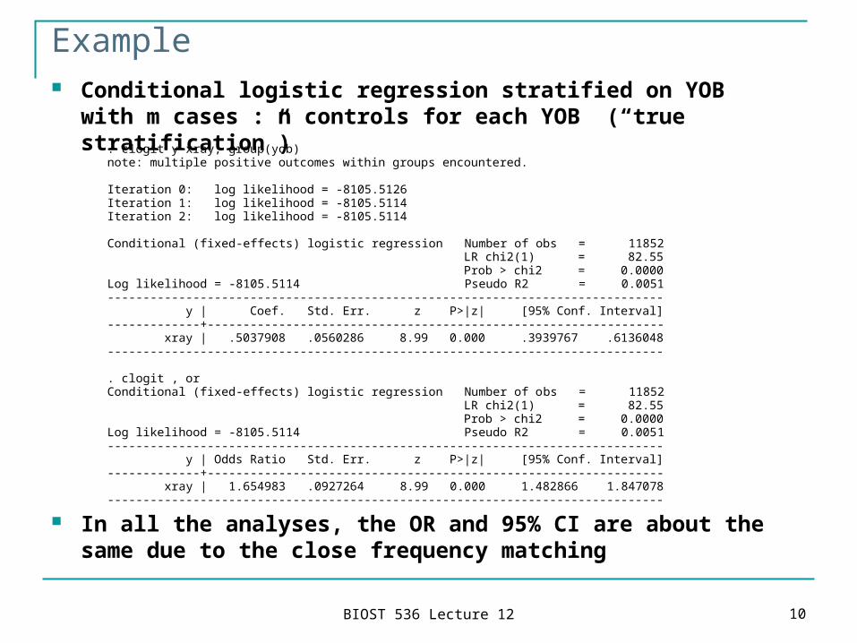
Example Conditional logistic regression stratified on YOB

with m cases : n controls for each YOB (“true stratification”)

In all the analyses, the OR and 95% CI are about the same due to the close frequency matching

. clogit y xray, group(yob) note: multiple positive outcomes within groups encountered. Iteration 0: log likelihood = -8105.5126 Iteration 1: log likelihood = -8105.5114 Iteration 2: log likelihood = -8105.5114 Conditional (fixed-effects) logistic regression Number of obs = 11852 LR chi2(1) = 82.55 Prob > chi2 = 0.0000 Log likelihood = -8105.5114 Pseudo R2 = 0.0051 ------------------------------------------------------------------------------ y | Coef. Std. Err. z P>|z| [95% Conf. Interval] -------------+---------------------------------------------------------------- xray | .5037908 .0560286 8.99 0.000 .3939767 .6136048 ------------------------------------------------------------------------------ . clogit , or Conditional (fixed-effects) logistic regression Number of obs = 11852 LR chi2(1) = 82.55 Prob > chi2 = 0.0000 Log likelihood = -8105.5114 Pseudo R2 = 0.0051 ------------------------------------------------------------------------------ y | Odds Ratio Std. Err. z P>|z| [95% Conf. Interval] -------------+---------------------------------------------------------------- xray | 1.654983 .0927264 8.99 0.000 1.482866 1.847078 ------------------------------------------------------------------------------

BIOST 536 Lecture 12 11

Conditional logistic regression

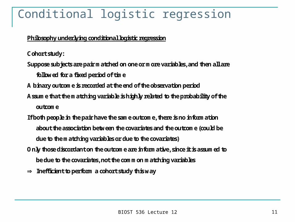
Philosophy underlying conditional logistic regression

Cohort study:

Suppose subjects are pair matched on one or more variables, and then all are

followed for a fixed period of time

A binary outcome is recorded at the end of the observation period

Assume that the matching variable is highly related to the probability of the

outcome

If both people in the pair have the same outcome, there is no information

about the association between the covariates and the outcome (could be

due to the matching variables or due to the covariates)

Only those discordant on the outcome are informative, since it is assumed to

be due to the covariates, not the common matching variables

Inefficient to perform a cohort study this way

BIOST 536 Lecture 12 12

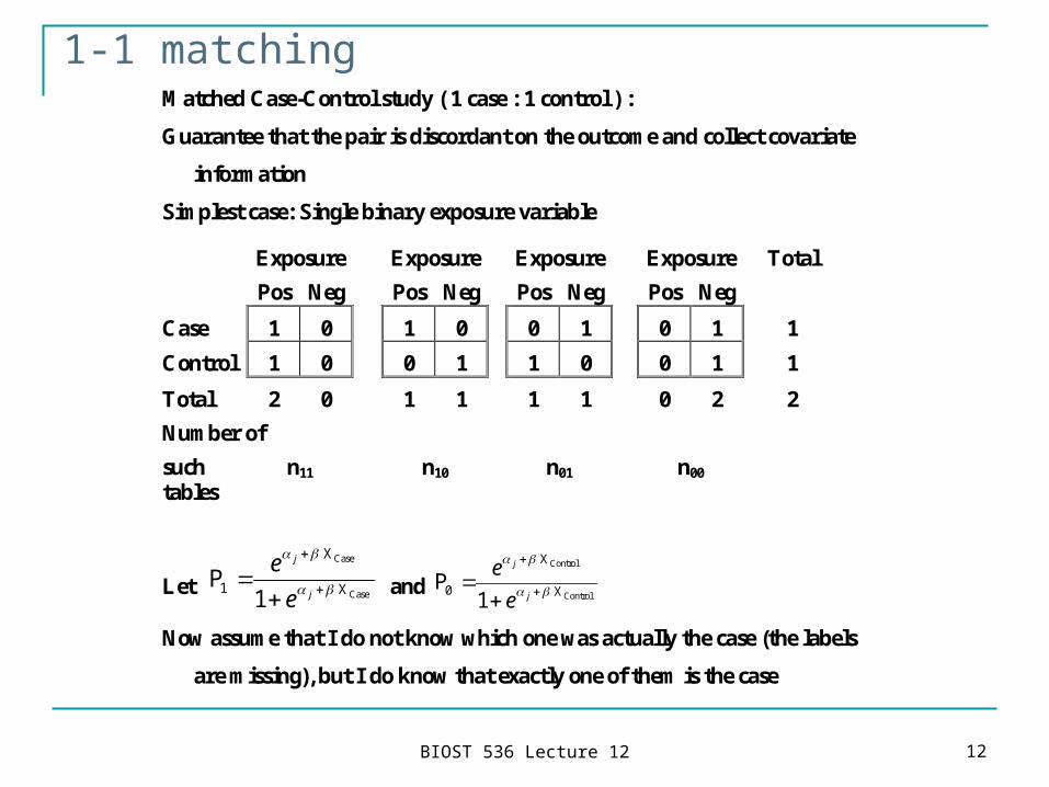
1-1 matchingMatched Case-Control study ( 1 case : 1 control ) :

Guarantee that the pair is discordant on the outcome and collect covariate

information

Simplest case: Single binary exposure variable

Exposure Exposure Exposure Exposure Total

Pos Neg Pos Neg Pos Neg Pos Neg

Case 1 0 1 0 0 1 0 1 1

Control 1 0 0 1 1 0 0 1 1

Total 2 0 1 1 1 1 0 2 2

Number of

such tables

n11 n10 n01 n00

Let P1

X

X

Case

Case

e

e

j

j

1 and P0

X

X

Control

Control

e

e

j

j

1

Now assume that I do not know which one was actually the case (the labels

are missing), but I do know that exactly one of them is the case

BIOST 536 Lecture 12 13

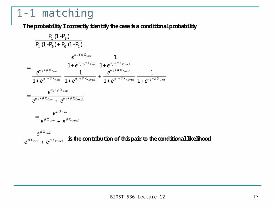
1-1 matchingThe probability I correctly identify the case is a conditional probability

P (1- P

P (1- P P (1- P1 0

1 0 0 1

)

) )

e

e ee

e e

e

e e

j

j j

j

j j

j

j j

X

X X

X

X X

X

X X

Case

Case Control

Case

Case Control

Control

Control Case

1

1

1

1

1

1 1

1

1

e

e e

j

j j

X

X X

Case

Case Control

e

e e

X

X X

Case

Case Control

e

e e

X

X X

Case

Case Control is the contribution of this pair to the conditional likelihood

BIOST 536 Lecture 12 14

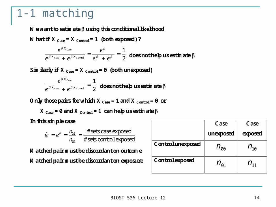
1-1 matchingWe want to estimate using this conditional likelihood

What if X Case = X Control = 1 (both exposed) ?

e

e e

e

e e

X

X X

Case

Case Control

1

2 does not help us estimate

Similarly if X Case = X Control = 0 (both unexposed)

e

e e

X

X X

Case

Case Control

1

2 does not help us estimate

Only those pairs for which X Case = 1 and X Control = 0 or

X Case = 0 and X Control = 1 can help us estimate

In this simple case

e

n

n10

01

#sets case exposed

#sets control exposed

Matched pair must be discordant on outcome

Matched pair must be discordant on exposure

Case

unexposed

Case

exposed

Control unexposed 00n 10n

Control exposed 01n 11n

BIOST 536 Lecture 12 15

1-1 matching

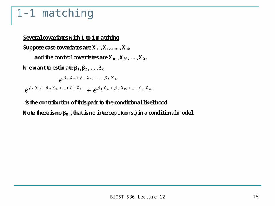
Several covariates with 1 to 1 matching

Suppose case covariates are X11, X12, ... , X1k

and the control covariates are X01, X02, ... , X0k

We want to estimate 1, 2, ... , k

e

e e

k

k k

1 2

1 2 1 2

X X X

X X X X X X

11 12 1k

11 12 1k 01 02 0k

...

... ...

is the contribution of this pair to the conditional likelihood

Note there is no 0 , that is no intercept (const) in a conditional model

BIOST 536 Lecture 12 16

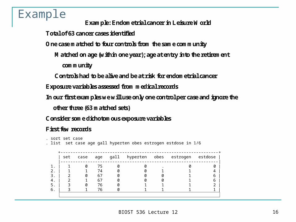
ExampleExample: Endometrial cancer in Leisure World

Total of 63 cancer cases identified

One case matched to four controls from the same community

Matched on age (within one year); age at entry into the retirement

community

Controls had to be alive and be at risk for endometrial cancer

Exposure variables assessed from medical records

In our first examples we will use only one control per case and ignore the

other three (63 matched sets)

Consider some dichotomous exposure variables

First few records . sort set case . list set case age gall hyperten obes estrogen estdose in 1/6 +----------------------------------------------------------------+ | set case age gall hyperten obes estrogen estdose | |----------------------------------------------------------------| 1. | 1 0 75 0 0 . 0 0 | 2. | 1 1 74 0 0 1 1 4 | 3. | 2 0 67 0 0 0 1 6 | 4. | 2 1 67 0 0 0 1 6 | 5. | 3 0 76 0 1 1 1 2 | 6. | 3 1 76 0 1 1 1 1 |

BIOST 536 Lecture 12 17

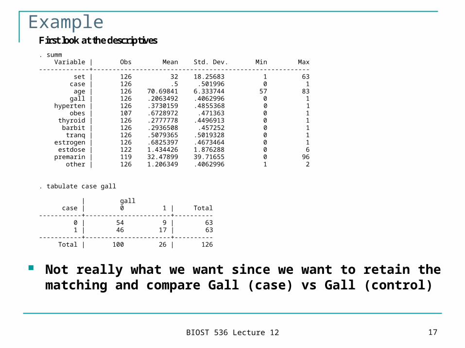
Example

Not really what we want since we want to retain the matching and compare Gall (case) vs Gall (control)

First look at the descriptives . summ Variable | Obs Mean Std. Dev. Min Max -------------+-------------------------------------------------------- set | 126 32 18.25683 1 63 case | 126 .5 .501996 0 1 age | 126 70.69841 6.333744 57 83 gall | 126 .2063492 .4062996 0 1 hyperten | 126 .3730159 .4855368 0 1 obes | 107 .6728972 .471363 0 1 thyroid | 126 .2777778 .4496913 0 1 barbit | 126 .2936508 .457252 0 1 tranq | 126 .5079365 .5019328 0 1 estrogen | 126 .6825397 .4673464 0 1 estdose | 122 1.434426 1.876288 0 6 premarin | 119 32.47899 39.71655 0 96 other | 126 1.206349 .4062996 1 2 . tabulate case gall | gall case | 0 1 | Total -----------+----------------------+---------- 0 | 54 9 | 63 1 | 46 17 | 63 -----------+----------------------+---------- Total | 100 26 | 126

BIOST 536 Lecture 12 18

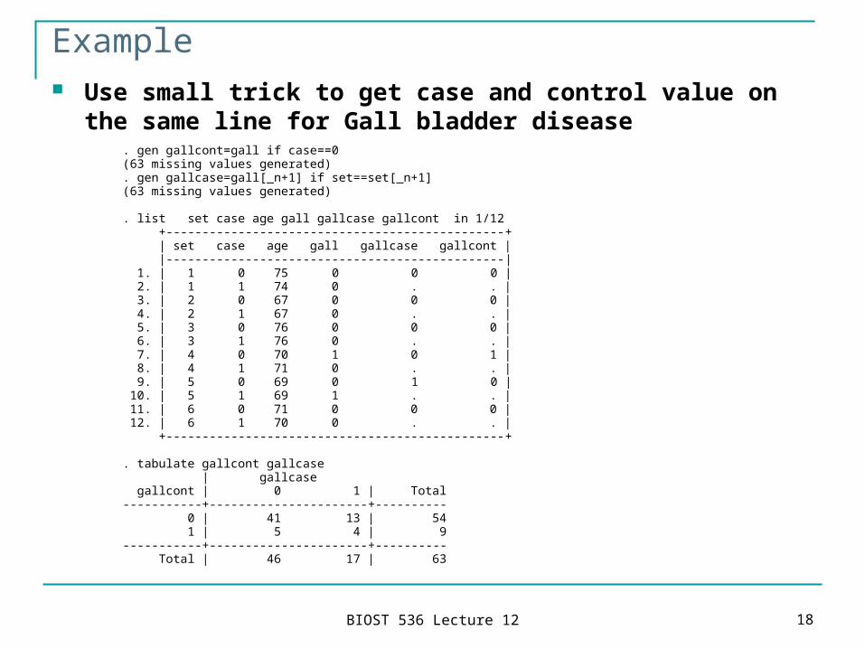
Example Use small trick to get case and control value on the same line

for Gall bladder disease. gen gallcont=gall if case==0 (63 missing values generated) . gen gallcase=gall[_n+1] if set==set[_n+1] (63 missing values generated) . list set case age gall gallcase gallcont in 1/12 +-----------------------------------------------+ | set case age gall gallcase gallcont | |-----------------------------------------------| 1. | 1 0 75 0 0 0 | 2. | 1 1 74 0 . . | 3. | 2 0 67 0 0 0 | 4. | 2 1 67 0 . . | 5. | 3 0 76 0 0 0 | 6. | 3 1 76 0 . . | 7. | 4 0 70 1 0 1 | 8. | 4 1 71 0 . . | 9. | 5 0 69 0 1 0 | 10. | 5 1 69 1 . . | 11. | 6 0 71 0 0 0 | 12. | 6 1 70 0 . . | +-----------------------------------------------+ . tabulate gallcont gallcase | gallcase gallcont | 0 1 | Total -----------+----------------------+---------- 0 | 41 13 | 54 1 | 5 4 | 9 -----------+----------------------+---------- Total | 46 17 | 63

BIOST 536 Lecture 12 19

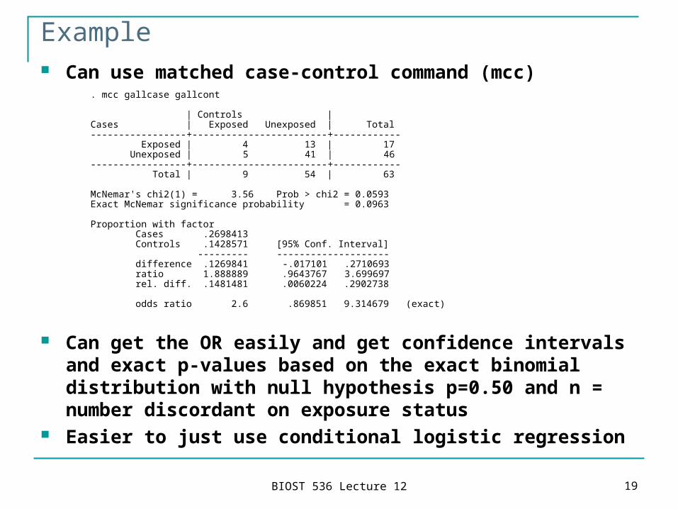
Example Can use matched case-control command (mcc)

Can get the OR easily and get confidence intervals and exact p-values based on the exact binomial distribution with null hypothesis p=0.50 and n = number discordant on exposure status

Easier to just use conditional logistic regression

. mcc gallcase gallcont | Controls | Cases | Exposed Unexposed | Total -----------------+------------------------+------------ Exposed | 4 13 | 17 Unexposed | 5 41 | 46 -----------------+------------------------+------------ Total | 9 54 | 63 McNemar's chi2(1) = 3.56 Prob > chi2 = 0.0593 Exact McNemar significance probability = 0.0963 Proportion with factor Cases .2698413 Controls .1428571 [95% Conf. Interval] --------- -------------------- difference .1269841 -.017101 .2710693 ratio 1.888889 .9643767 3.699697 rel. diff. .1481481 .0060224 .2902738 odds ratio 2.6 .869851 9.314679 (exact)

BIOST 536 Lecture 12 20

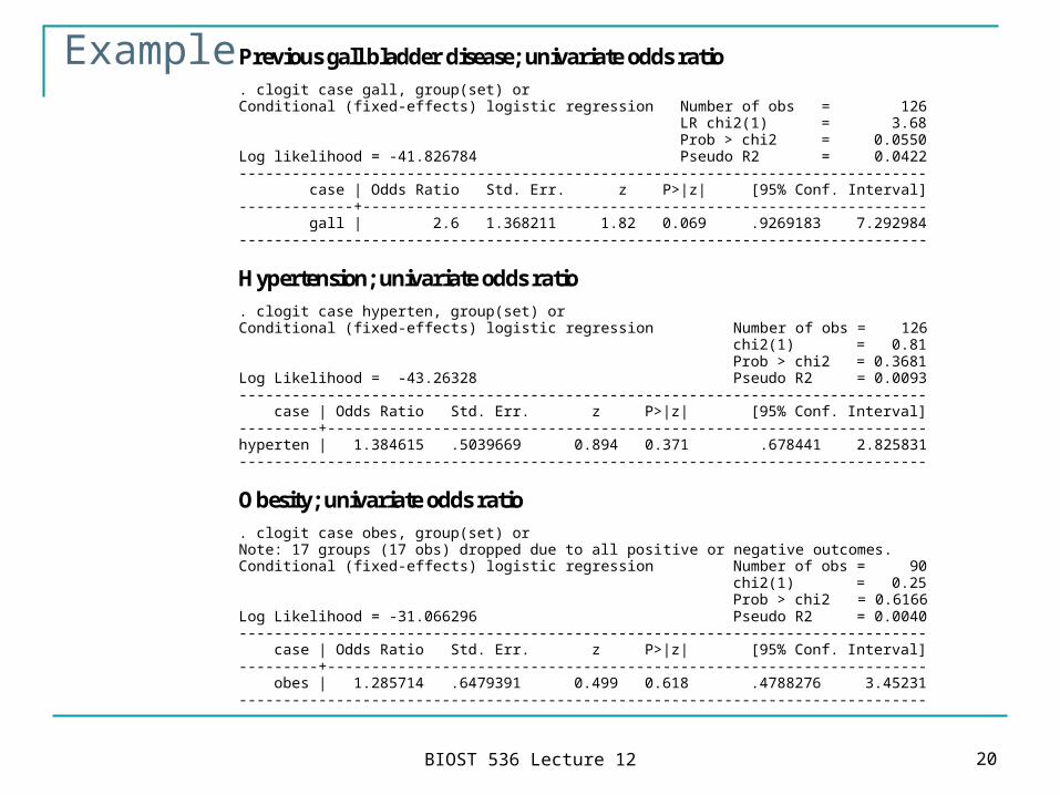
ExamplePrevious gall bladder disease; univariate odds ratio . clogit case gall, group(set) or Conditional (fixed-effects) logistic regression Number of obs = 126 LR chi2(1) = 3.68 Prob > chi2 = 0.0550 Log likelihood = -41.826784 Pseudo R2 = 0.0422 ------------------------------------------------------------------------------ case | Odds Ratio Std. Err. z P>|z| [95% Conf. Interval] -------------+---------------------------------------------------------------- gall | 2.6 1.368211 1.82 0.069 .9269183 7.292984 ------------------------------------------------------------------------------

Hypertension; univariate odds ratio . clogit case hyperten, group(set) or Conditional (fixed-effects) logistic regression Number of obs = 126 chi2(1) = 0.81 Prob > chi2 = 0.3681 Log Likelihood = -43.26328 Pseudo R2 = 0.0093 ------------------------------------------------------------------------------ case | Odds Ratio Std. Err. z P>|z| [95% Conf. Interval] ---------+-------------------------------------------------------------------- hyperten | 1.384615 .5039669 0.894 0.371 .678441 2.825831 ------------------------------------------------------------------------------

Obesity; univariate odds ratio . clogit case obes, group(set) or Note: 17 groups (17 obs) dropped due to all positive or negative outcomes. Conditional (fixed-effects) logistic regression Number of obs = 90 chi2(1) = 0.25 Prob > chi2 = 0.6166 Log Likelihood = -31.066296 Pseudo R2 = 0.0040 ------------------------------------------------------------------------------ case | Odds Ratio Std. Err. z P>|z| [95% Conf. Interval] ---------+-------------------------------------------------------------------- obes | 1.285714 .6479391 0.499 0.618 .4788276 3.45231 ------------------------------------------------------------------------------

BIOST 536 Lecture 12 21

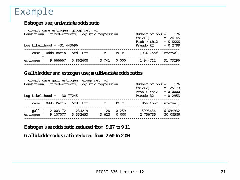
ExampleEstrogen use; univariate odds ratio . clogit case estrogen, group(set) or Conditional (fixed-effects) logistic regression Number of obs = 126 chi2(1) = 24.45 Prob > chi2 = 0.0000 Log Likelihood = -31.443696 Pseudo R2 = 0.2799 ------------------------------------------------------------------------------ case | Odds Ratio Std. Err. z P>|z| [95% Conf. Interval] ---------+-------------------------------------------------------------------- estrogen | 9.666667 5.862608 3.741 0.000 2.944712 31.73296 ------------------------------------------------------------------------------

Gall bladder and estrogen use; multivariate odds ratios . clogit case gall estrogen, group(set) or Conditional (fixed-effects) logistic regression Number of obs = 126 chi2(2) = 25.79 Prob > chi2 = 0.0000 Log Likelihood = -30.77245 Pseudo R2 = 0.2953 ------------------------------------------------------------------------------ case | Odds Ratio Std. Err. z P>|z| [95% Conf. Interval] ---------+-------------------------------------------------------------------- gall | 2.003172 1.233219 1.128 0.259 .5993636 6.694932 estrogen | 9.107077 5.552653 3.623 0.000 2.756735 30.08589 ------------------------------------------------------------------------------

Estrogen use odds ratio reduced from 9.67 to 9.11

Gall bladder odds ratio reduced from 2.60 to 2.00

BIOST 536 Lecture 12 22

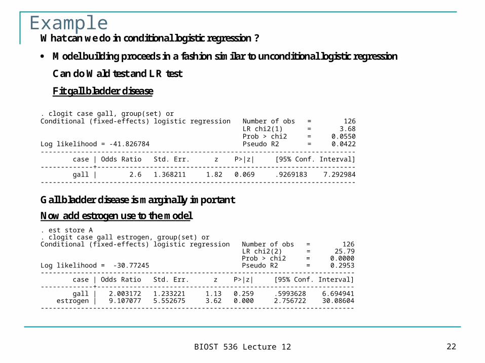
ExampleWhat can we do in conditional logistic regression ?

Model building proceeds in a fashion similar to unconditional logistic regression

Can do Wald test and LR test

Fit gall bladder disease . clogit case gall, group(set) or Conditional (fixed-effects) logistic regression Number of obs = 126 LR chi2(1) = 3.68 Prob > chi2 = 0.0550 Log likelihood = -41.826784 Pseudo R2 = 0.0422 ------------------------------------------------------------------------------ case | Odds Ratio Std. Err. z P>|z| [95% Conf. Interval] -------------+---------------------------------------------------------------- gall | 2.6 1.368211 1.82 0.069 .9269183 7.292984 ------------------------------------------------------------------------------

Gall bladder disease is marginally important

Now add estrogen use to the model . est store A . clogit case gall estrogen, group(set) or Conditional (fixed-effects) logistic regression Number of obs = 126 LR chi2(2) = 25.79 Prob > chi2 = 0.0000 Log likelihood = -30.77245 Pseudo R2 = 0.2953 ------------------------------------------------------------------------------ case | Odds Ratio Std. Err. z P>|z| [95% Conf. Interval] -------------+---------------------------------------------------------------- gall | 2.003172 1.233221 1.13 0.259 .5993628 6.694941 estrogen | 9.107077 5.552675 3.62 0.000 2.756722 30.08604 ------------------------------------------------------------------------------

BIOST 536 Lecture 12 23

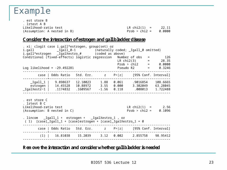
Example. est store B . lrtest A B Likelihood-ratio test LR chi2(1) = 22.11 (Assumption: A nested in B) Prob > chi2 = 0.0000

Consider the interaction of estrogen and gall bladder disease . xi: clogit case i.gall*estrogen, group(set) or i.gall _Igall_0-1 (naturally coded; _Igall_0 omitted) i.gall*estrogen _IgalXestro_# (coded as above) Conditional (fixed-effects) logistic regression Number of obs = 126 LR chi2(3) = 28.35 Prob > chi2 = 0.0000 Log likelihood = -29.492281 Pseudo R2 = 0.3246 ------------------------------------------------------------------------------ case | Odds Ratio Std. Err. z P>|z| [95% Conf. Interval] -------------+---------------------------------------------------------------- _Igall_1 | 9.898637 12.10023 1.88 0.061 .9016854 108.6665 estrogen | 14.45528 10.88972 3.55 0.000 3.302049 63.28045 _IgalXestr~1 | .1174832 .1609567 -1.56 0.118 .008013 1.722488 ------------------------------------------------------------------------------ . est store C . lrtest B C Likelihood-ratio test LR chi2(1) = 2.56 (Assumption: B nested in C) Prob > chi2 = 0.1096 . lincom _Igall_1 + estrogen + _IgalXestro_1 , or ( 1) [case]_Igall_1 + [case]estrogen + [case]_IgalXestro_1 = 0 ------------------------------------------------------------------------------ case | Odds Ratio Std. Err. z P>|z| [95% Conf. Interval] -------------+---------------------------------------------------------------- (1) | 16.81038 15.2039 3.12 0.002 2.855758 98.95412 ------------------------------------------------------------------------------

Remove the interaction and consider whether gall bladder is needed

BIOST 536 Lecture 12 24

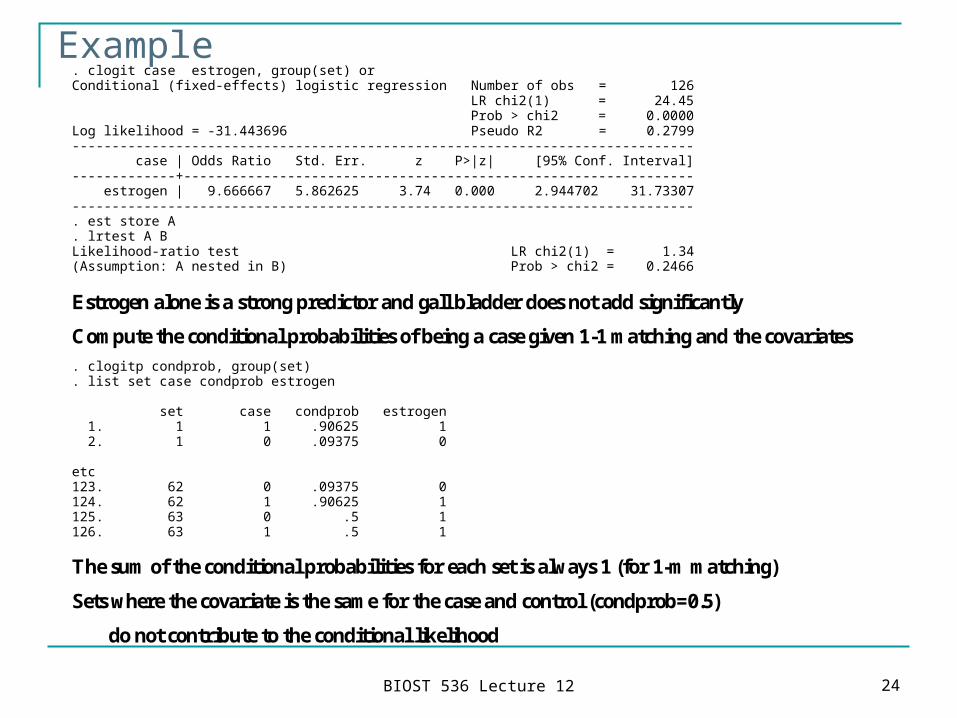
Example. clogit case estrogen, group(set) or Conditional (fixed-effects) logistic regression Number of obs = 126 LR chi2(1) = 24.45 Prob > chi2 = 0.0000 Log likelihood = -31.443696 Pseudo R2 = 0.2799 ------------------------------------------------------------------------------ case | Odds Ratio Std. Err. z P>|z| [95% Conf. Interval] -------------+---------------------------------------------------------------- estrogen | 9.666667 5.862625 3.74 0.000 2.944702 31.73307 ------------------------------------------------------------------------------ . est store A . lrtest A B Likelihood-ratio test LR chi2(1) = 1.34 (Assumption: A nested in B) Prob > chi2 = 0.2466

Estrogen alone is a strong predictor and gall bladder does not add significantly

Compute the conditional probabilities of being a case given 1-1 matching and the covariates . clogitp condprob, group(set) . list set case condprob estrogen set case condprob estrogen 1. 1 1 .90625 1 2. 1 0 .09375 0 etc 123. 62 0 .09375 0 124. 62 1 .90625 1 125. 63 0 .5 1 126. 63 1 .5 1

The sum of the conditional probabilities for each set is always 1 (for 1-m matching)

Sets where the covariate is the same for the case and control (condprob=0.5)

do not contribute to the conditional likelihood

BIOST 536 Lecture 12 25

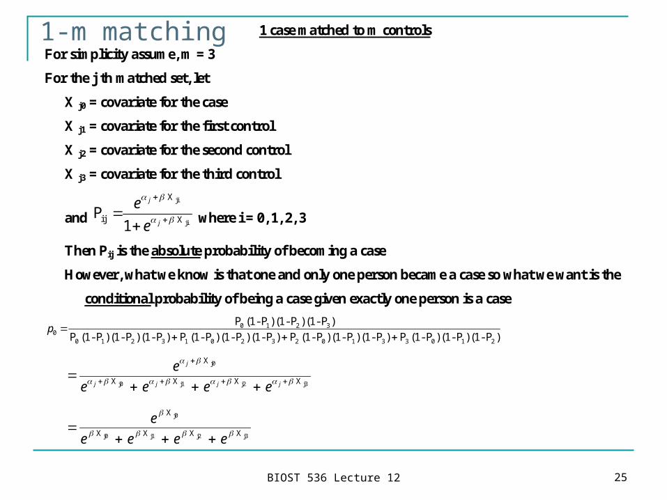
1-m matching 1 case matched to m controls

For simplicity assume, m = 3

For the j th matched set, let

X j0 = covariate for the case

X j1 = covariate for the first control

X j2 = covariate for the second control

X j3 = covariate for the third control

and Pij

X

X

ji

ji

e

e

j

j

1 where i = 0, 1, 2, 3

Then Pij is the absolute probability of becoming a case

However, what we know is that one and only one person became a case so what we want is the

conditional probability of being a case given exactly one person is a case

p00 1 2 3

0 1 2 3 1 0 2 3 2 0 1 3 3 0 1 2

P (1- P (1- P (1- P

P (1- P (1- P (1- P P (1- P (1- P (1- P P (1- P (1- P (1- P P (1- P (1- P (1- P

) ) )

) ) ) ) ) ) ) ) ) ) ) )

e

e e e e

j

j j j j

X

X X X X

j0

j0 j1 j2 j3

e

e e e e

X

X X X X

j0

j0 j1 j2 j3

BIOST 536 Lecture 12 26

1-m matching Since j is not estimated, we can not get the unconditional probability Pij

We can estimate the conditional probabilities, i.e. p0, p1, p2, p3 , instead

These actually are multinomial probabilities

j3j2j1j0

j1

XXXX

X

1

eeee

ep

j3j2j1j0

j2

XXXX

X

2

eeee

ep

j3j2j1j0

j3

XXXX

X

3

eeee

ep

are the

conditional probabilities that each control was the one and only case in the set

Note: 13210 pppp by the way they are defined

If the covariate is the same for all members of the set we would have the likelihood contribution

4

1xxxx

x

XXXX

X

0 j3j2j1j0

j0

eeee

e

eeee

ep

so would not tell us anything about

If there are several covariates then the conditional probability for 1 to m matching is

e

e e

k

k k

1 2

1 2 1 2

X X X

X X X X X X

controls i=1 to m

j01 j02 j0k

j01 j02 j0k ji1 ji2 jik

...

... ...

BIOST 536 Lecture 12 27

1-m matching

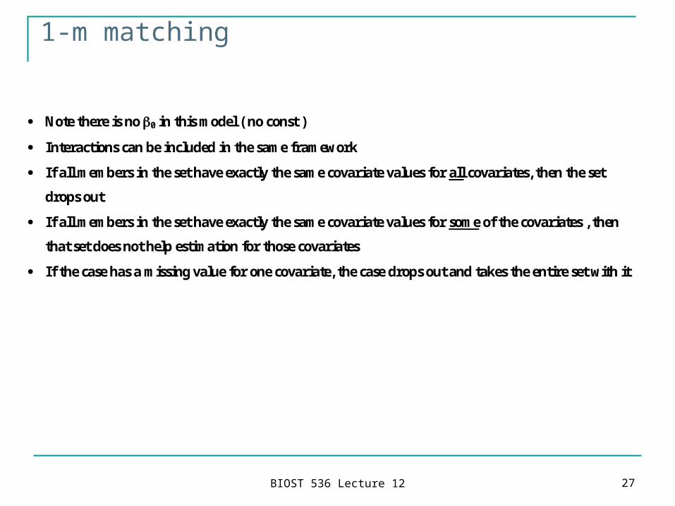
Note there is no 0 in this model ( no const )

Interactions can be included in the same framework

If all members in the set have exactly the same covariate values for all covariates, then the set

drops out

If all members in the set have exactly the same covariate values for some of the covariates , then

that set does not help estimation for those covariates

If the case has a missing value for one covariate, the case drops out and takes the entire set with it

BIOST 536 Lecture 12 28

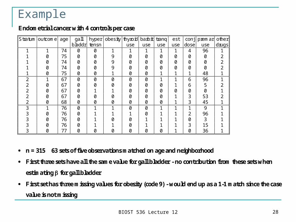
ExampleEndometrial cancer with 4 controls per case

Stratum outcome age gall bladdr

hyper tensn

obesity thyroid use

barbit use

tranq use

est use

conj dose

premar use

other drugs

1 1 74 0 0 1 1 1 1 1 4 96 1 1 0 75 0 0 9 0 0 0 0 0 0 2 1 0 74 0 0 9 0 0 0 0 0 0 2 1 0 74 0 0 9 0 0 0 0 0 0 2 1 0 75 0 0 1 0 0 1 1 1 48 1 2 1 67 0 0 0 0 0 1 1 6 96 1 2 0 67 0 0 0 0 0 0 1 6 5 2 2 0 67 0 1 1 0 0 0 0 0 0 1 2 0 67 0 0 0 0 0 0 1 3 53 2 2 0 68 0 0 0 0 0 0 1 3 45 1 3 1 76 0 1 1 0 0 1 1 1 9 1 3 0 76 0 1 1 1 0 1 1 2 96 1 3 0 76 0 1 0 0 1 1 1 0 3 1 3 0 76 0 1 1 0 1 1 1 3 15 1 3 0 77 0 0 0 0 0 0 1 0 36 1

n = 315 63 sets of five observations matched on age and neighborhood

First three sets have all the same value for gall bladder - no contribution from these sets when

estimating for gall bladder

First set has three missing values for obesity (code 9) - would end up as a 1-1 match since the case

value is not missing

BIOST 536 Lecture 12 29

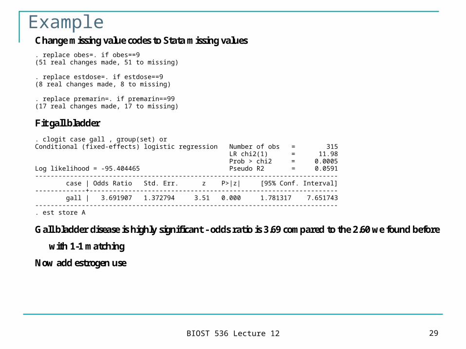
ExampleChange missing value codes to Stata missing values . replace obes=. if obes==9 (51 real changes made, 51 to missing) . replace estdose=. if estdose==9 (8 real changes made, 8 to missing) . replace premarin=. if premarin==99 (17 real changes made, 17 to missing)

Fit gall bladder . clogit case gall , group(set) or Conditional (fixed-effects) logistic regression Number of obs = 315 LR chi2(1) = 11.98 Prob > chi2 = 0.0005 Log likelihood = -95.404465 Pseudo R2 = 0.0591 ------------------------------------------------------------------------------ case | Odds Ratio Std. Err. z P>|z| [95% Conf. Interval] -------------+---------------------------------------------------------------- gall | 3.691907 1.372794 3.51 0.000 1.781317 7.651743 ------------------------------------------------------------------------------ . est store A

Gall bladder disease is highly significant - odds ratio is 3.69 compared to the 2.60 we found before

with 1-1 matching

Now add estrogen use

BIOST 536 Lecture 12 30

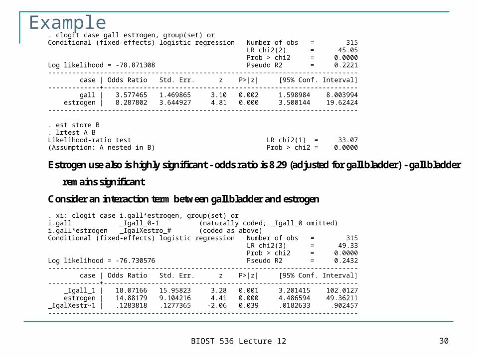
Example. clogit case gall estrogen, group(set) or Conditional (fixed-effects) logistic regression Number of obs = 315 LR chi2(2) = 45.05 Prob > chi2 = 0.0000 Log likelihood = -78.871308 Pseudo R2 = 0.2221 ------------------------------------------------------------------------------ case | Odds Ratio Std. Err. z P>|z| [95% Conf. Interval] -------------+---------------------------------------------------------------- gall | 3.577465 1.469865 3.10 0.002 1.598984 8.003994 estrogen | 8.287802 3.644927 4.81 0.000 3.500144 19.62424 ------------------------------------------------------------------------------ . est store B . lrtest A B Likelihood-ratio test LR chi2(1) = 33.07 (Assumption: A nested in B) Prob > chi2 = 0.0000

Estrogen use also is highly significant - odds ratio is 8.29 (adjusted for gall bladder) - gall bladder

remains significant

Consider an interaction term between gall bladder and estrogen . xi: clogit case i.gall*estrogen, group(set) or i.gall _Igall_0-1 (naturally coded; _Igall_0 omitted) i.gall*estrogen _IgalXestro_# (coded as above) Conditional (fixed-effects) logistic regression Number of obs = 315 LR chi2(3) = 49.33 Prob > chi2 = 0.0000 Log likelihood = -76.730576 Pseudo R2 = 0.2432 ------------------------------------------------------------------------------ case | Odds Ratio Std. Err. z P>|z| [95% Conf. Interval] -------------+---------------------------------------------------------------- _Igall_1 | 18.07166 15.95823 3.28 0.001 3.201415 102.0127 estrogen | 14.88179 9.104216 4.41 0.000 4.486594 49.36211 _IgalXestr~1 | .1283818 .1277365 -2.06 0.039 .0182633 .902457 ------------------------------------------------------------------------------

BIOST 536 Lecture 12 31

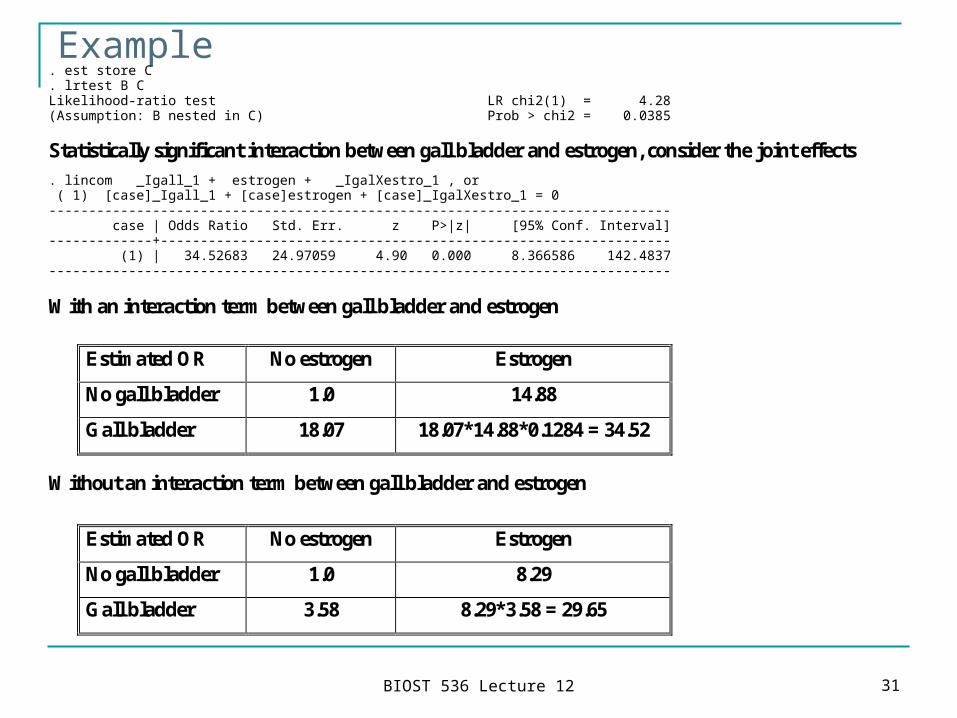
Example. est store C . lrtest B C Likelihood-ratio test LR chi2(1) = 4.28 (Assumption: B nested in C) Prob > chi2 = 0.0385

Statistically significant interaction between gall bladder and estrogen, consider the joint effects . lincom _Igall_1 + estrogen + _IgalXestro_1 , or ( 1) [case]_Igall_1 + [case]estrogen + [case]_IgalXestro_1 = 0 ------------------------------------------------------------------------------ case | Odds Ratio Std. Err. z P>|z| [95% Conf. Interval] -------------+---------------------------------------------------------------- (1) | 34.52683 24.97059 4.90 0.000 8.366586 142.4837 ------------------------------------------------------------------------------

With an interaction term between gall bladder and estrogen

Estimated OR No estrogen Estrogen

No gall bladder 1.0 14.88

Gall bladder 18.07 18.07*14.88*0.1284 = 34.52

Without an interaction term between gall bladder and estrogen

Estimated OR No estrogen Estrogen

No gall bladder 1.0 8.29

Gall bladder 3.58 8.29*3.58 = 29.65

BIOST 536 Lecture 12 32

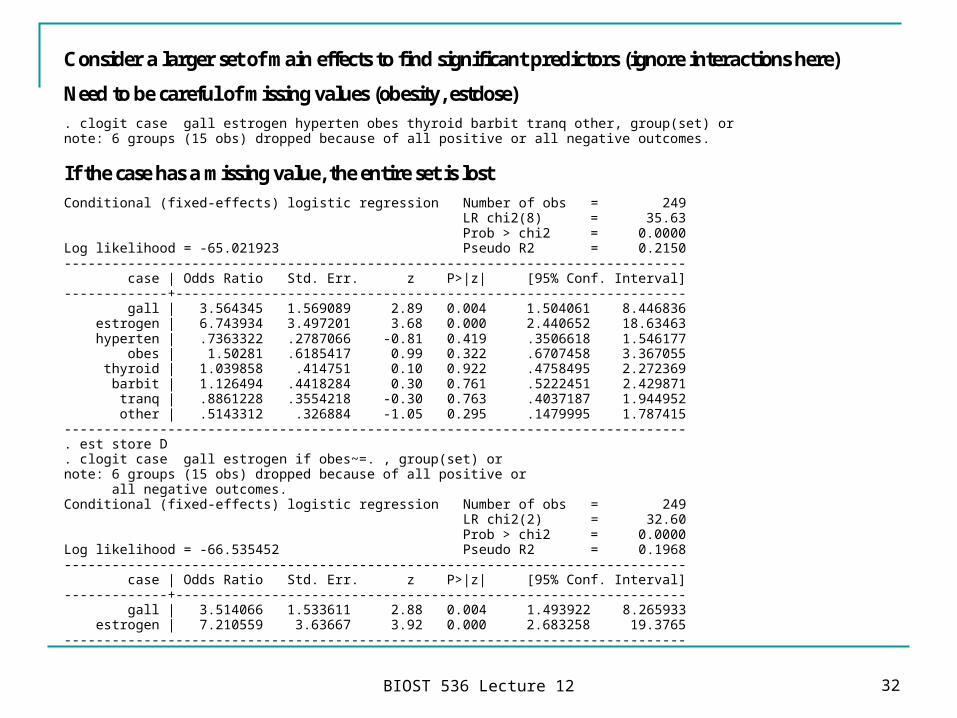
Consider a larger set of main effects to find significant predictors (ignore interactions here)

Need to be careful of missing values (obesity, estdose) . clogit case gall estrogen hyperten obes thyroid barbit tranq other, group(set) or note: 6 groups (15 obs) dropped because of all positive or all negative outcomes.

If the case has a missing value, the entire set is lost Conditional (fixed-effects) logistic regression Number of obs = 249 LR chi2(8) = 35.63 Prob > chi2 = 0.0000 Log likelihood = -65.021923 Pseudo R2 = 0.2150 ------------------------------------------------------------------------------ case | Odds Ratio Std. Err. z P>|z| [95% Conf. Interval] -------------+---------------------------------------------------------------- gall | 3.564345 1.569089 2.89 0.004 1.504061 8.446836 estrogen | 6.743934 3.497201 3.68 0.000 2.440652 18.63463 hyperten | .7363322 .2787066 -0.81 0.419 .3506618 1.546177 obes | 1.50281 .6185417 0.99 0.322 .6707458 3.367055 thyroid | 1.039858 .414751 0.10 0.922 .4758495 2.272369 barbit | 1.126494 .4418284 0.30 0.761 .5222451 2.429871 tranq | .8861228 .3554218 -0.30 0.763 .4037187 1.944952 other | .5143312 .326884 -1.05 0.295 .1479995 1.787415 ------------------------------------------------------------------------------ . est store D . clogit case gall estrogen if obes~=. , group(set) or note: 6 groups (15 obs) dropped because of all positive or all negative outcomes. Conditional (fixed-effects) logistic regression Number of obs = 249 LR chi2(2) = 32.60 Prob > chi2 = 0.0000 Log likelihood = -66.535452 Pseudo R2 = 0.1968 ------------------------------------------------------------------------------ case | Odds Ratio Std. Err. z P>|z| [95% Conf. Interval] -------------+---------------------------------------------------------------- gall | 3.514066 1.533611 2.88 0.004 1.493922 8.265933 estrogen | 7.210559 3.63667 3.92 0.000 2.683258 19.3765 ------------------------------------------------------------------------------

BIOST 536 Lecture 12 33

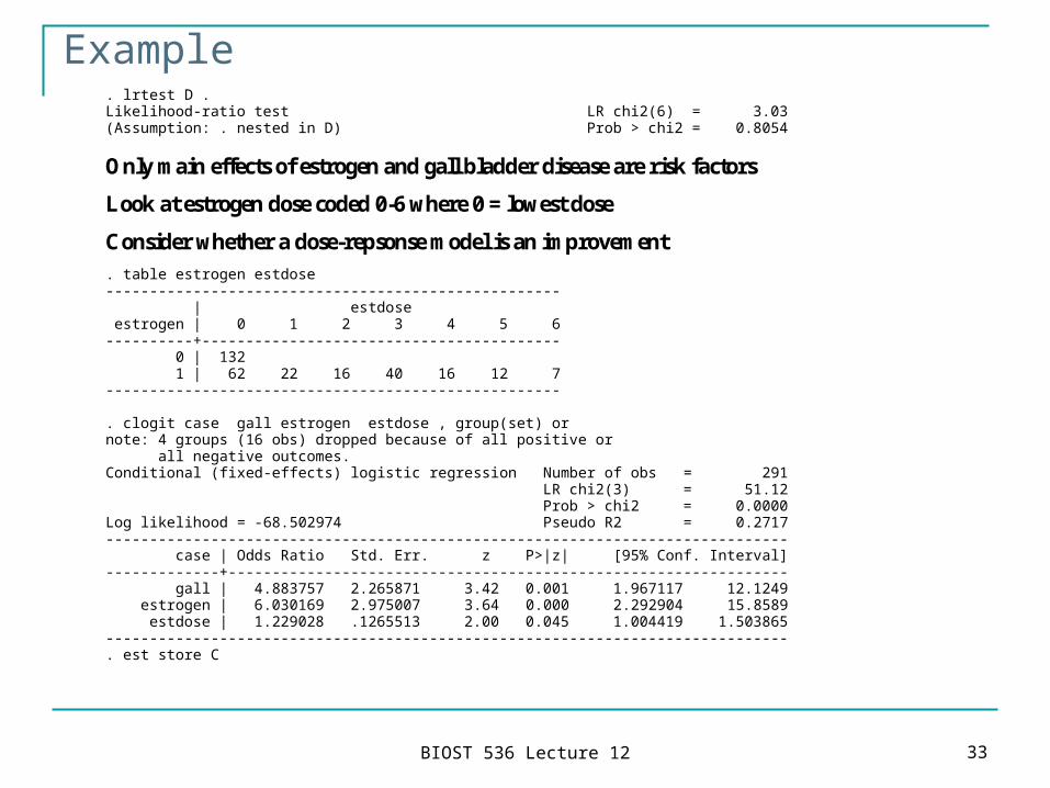
Example. lrtest D . Likelihood-ratio test LR chi2(6) = 3.03 (Assumption: . nested in D) Prob > chi2 = 0.8054

Only main effects of estrogen and gall bladder disease are risk factors

Look at estrogen dose coded 0-6 where 0 = lowest dose

Consider whether a dose-repsonse model is an improvement . table estrogen estdose ---------------------------------------------------- | estdose estrogen | 0 1 2 3 4 5 6 ----------+----------------------------------------- 0 | 132 1 | 62 22 16 40 16 12 7 ---------------------------------------------------- . clogit case gall estrogen estdose , group(set) or note: 4 groups (16 obs) dropped because of all positive or all negative outcomes. Conditional (fixed-effects) logistic regression Number of obs = 291 LR chi2(3) = 51.12 Prob > chi2 = 0.0000 Log likelihood = -68.502974 Pseudo R2 = 0.2717 ------------------------------------------------------------------------------ case | Odds Ratio Std. Err. z P>|z| [95% Conf. Interval] -------------+---------------------------------------------------------------- gall | 4.883757 2.265871 3.42 0.001 1.967117 12.1249 estrogen | 6.030169 2.975007 3.64 0.000 2.292904 15.8589 estdose | 1.229028 .1265513 2.00 0.045 1.004419 1.503865 ------------------------------------------------------------------------------ . est store C

BIOST 536 Lecture 12 34

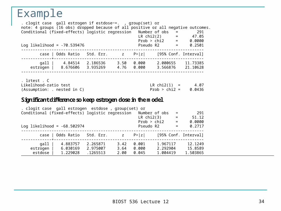
Example. clogit case gall estrogen if estdose~=. , group(set) or note: 4 groups (16 obs) dropped because of all positive or all negative outcomes. Conditional (fixed-effects) logistic regression Number of obs = 291 LR chi2(2) = 47.05 Prob > chi2 = 0.0000 Log likelihood = -70.539476 Pseudo R2 = 0.2501 ------------------------------------------------------------------------------ case | Odds Ratio Std. Err. z P>|z| [95% Conf. Interval] -------------+---------------------------------------------------------------- gall | 4.84514 2.186536 3.50 0.000 2.000655 11.73385 estrogen | 8.676606 3.935269 4.76 0.000 3.566876 21.10628 ------------------------------------------------------------------------------ . lrtest . C Likelihood-ratio test LR chi2(1) = 4.07 (Assumption: . nested in C) Prob > chi2 = 0.0436

Significant difference so keep estrogen dose in the model . clogit case gall estrogen estdose , group(set) or Conditional (fixed-effects) logistic regression Number of obs = 291 LR chi2(3) = 51.12 Prob > chi2 = 0.0000 Log likelihood = -68.502974 Pseudo R2 = 0.2717 ------------------------------------------------------------------------------ case | Odds Ratio Std. Err. z P>|z| [95% Conf. Interval] -------------+---------------------------------------------------------------- gall | 4.883757 2.265871 3.42 0.001 1.967117 12.1249 estrogen | 6.030169 2.975007 3.64 0.000 2.292904 15.8589 estdose | 1.229028 .1265513 2.00 0.045 1.004419 1.503865

BIOST 536 Lecture 12 35

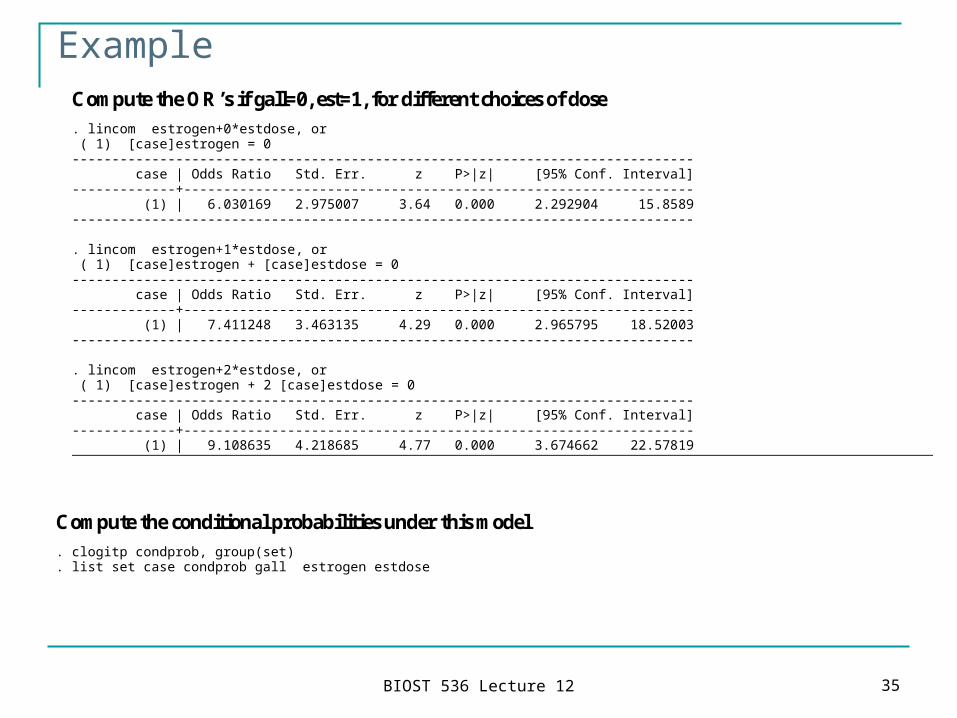
ExampleCompute the OR’s if gall=0, est=1, for different choices of dose . lincom estrogen+0*estdose, or ( 1) [case]estrogen = 0 ------------------------------------------------------------------------------ case | Odds Ratio Std. Err. z P>|z| [95% Conf. Interval] -------------+---------------------------------------------------------------- (1) | 6.030169 2.975007 3.64 0.000 2.292904 15.8589 ------------------------------------------------------------------------------ . lincom estrogen+1*estdose, or ( 1) [case]estrogen + [case]estdose = 0 ------------------------------------------------------------------------------ case | Odds Ratio Std. Err. z P>|z| [95% Conf. Interval] -------------+---------------------------------------------------------------- (1) | 7.411248 3.463135 4.29 0.000 2.965795 18.52003 ------------------------------------------------------------------------------ . lincom estrogen+2*estdose, or ( 1) [case]estrogen + 2 [case]estdose = 0 ------------------------------------------------------------------------------ case | Odds Ratio Std. Err. z P>|z| [95% Conf. Interval] -------------+---------------------------------------------------------------- (1) | 9.108635 4.218685 4.77 0.000 3.674662 22.57819

Compute the conditional probabilities under this model . clogitp condprob, group(set) . list set case condprob gall estrogen estdose

BIOST 536 Lecture 12 36

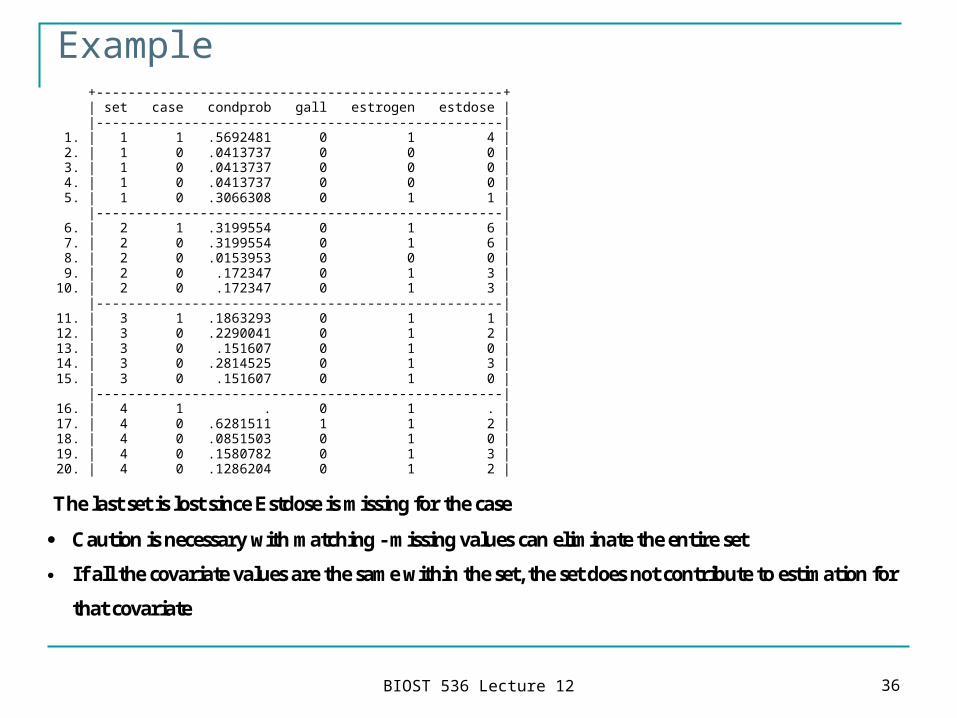
Example +---------------------------------------------------+ | set case condprob gall estrogen estdose | |---------------------------------------------------| 1. | 1 1 .5692481 0 1 4 | 2. | 1 0 .0413737 0 0 0 | 3. | 1 0 .0413737 0 0 0 | 4. | 1 0 .0413737 0 0 0 | 5. | 1 0 .3066308 0 1 1 | |---------------------------------------------------| 6. | 2 1 .3199554 0 1 6 | 7. | 2 0 .3199554 0 1 6 | 8. | 2 0 .0153953 0 0 0 | 9. | 2 0 .172347 0 1 3 | 10. | 2 0 .172347 0 1 3 | |---------------------------------------------------| 11. | 3 1 .1863293 0 1 1 | 12. | 3 0 .2290041 0 1 2 | 13. | 3 0 .151607 0 1 0 | 14. | 3 0 .2814525 0 1 3 | 15. | 3 0 .151607 0 1 0 | |---------------------------------------------------| 16. | 4 1 . 0 1 . | 17. | 4 0 .6281511 1 1 2 | 18. | 4 0 .0851503 0 1 0 | 19. | 4 0 .1580782 0 1 3 | 20. | 4 0 .1286204 0 1 2 |

The last set is lost since Estdose is missing for the case

Caution is necessary with matching - missing values can eliminate the entire set

If all the covariate values are the same within the set, the set does not contribute to estimation for

that covariate

BIOST 536 Lecture 12 37

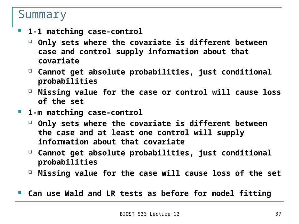
Summary 1-1 matching case-control

Only sets where the covariate is different between case and control supply information about that covariate

Cannot get absolute probabilities, just conditional probabilities

Missing value for the case or control will cause loss of the set

1-m matching case-control Only sets where the covariate is different between the case

and at least one control will supply information about that covariate

Cannot get absolute probabilities, just conditional probabilities

Missing value for the case will cause loss of the set Can use Wald and LR tests as before for model fitting